HPC Computer Aided Engineering @ CINECA

Raffaele Ponzini Ph.D.

CINECA

SuperComputing Applications

and Innovation Department – SCAI

16-18 June 2014

Outline

• What is CFD

• CFD main concepts

• CFD main definitions

• How should I use it

Computational Fluid Dynamics: CFD

• Fluid dynamics: physics of fluids

• Computational: numerical engine involved in solving the equation describing the motion of the fluid by means of iterative methods

There is a strong interplay between math concepts, physics knowledge and technological tools and environments used to implement a CFD model.

Demanding task:

• No general rules for specific CFD model setup

• Need of a-priori knowledge of the fluid behavior

• Need of a-priori knowledge of the physics involved by the problem

• If possible experimental (or theoretical) data to validate CFD results

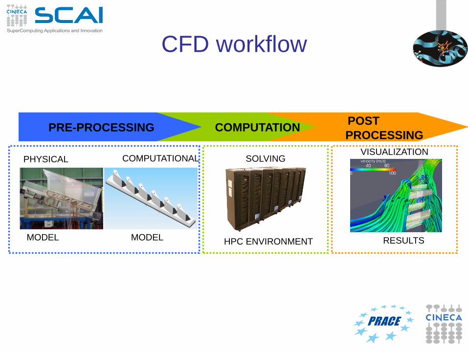
CFD workflow

PRE-PROCESSING COMPUTATION POST

PROCESSING

SOLVING

HPC ENVIRONMENT

COMPUTATIONAL VISUALIZATION

RESULTS MODEL MODEL

PHYSICAL

CFD: general approach

A very rough definition to explain how CFD works can be as follow:

“ CFD applies the principles of conservation of mass and

momentum according to the geometry and the mechanical

properties of the fluid involved by the problem to be able to get

information on instantaneous velocity and pressure distributions. “

Three pylons:

1. Geometry description

2. Fluid properties

3. Fluid conditions

Analytical (Exact) solution (integrals) is not available for

the specific geometry (CAD) but thanks to iterative

(Automated) methods a numerical (Approximated)

solution of the problem can be found.

Continuum Discrete

Math Numeric

Numeric Technology (HW, SW)

CFD: general idea

When moving from math to numeric we need to understand that

there is a counterpart version of each concept and that once we

move to numeric also technical issues comes in to play

Convergence

Consistency

Stability

Boundedness

Conservativeness

Transportiveness

Math || Numeric

CFD: general approach

When moving from math to numeric we need to understand that

there is a counterpart version of each concept and that once we

move to numeric also technical issues comes in to play

Theory Practice

Theory:

IF #cells (used to discretize the continuum) ∞

THEN the numerical solution ’exact’

and this will be independent from the numerical scheme adopted.

Practice:

IF #cells if finite

THEN the numerical solution ‘OK’

and this will be dependent from the properties of the numerical scheme adopted

Problem Discretization

This part of the workflow is the so-called

pre-processing and/or meshing process

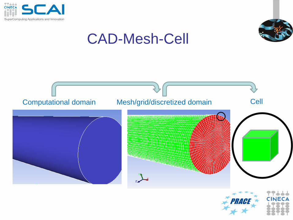
CAD-Mesh-Cell

Mesh/grid/discretized domain Cell Computational domain

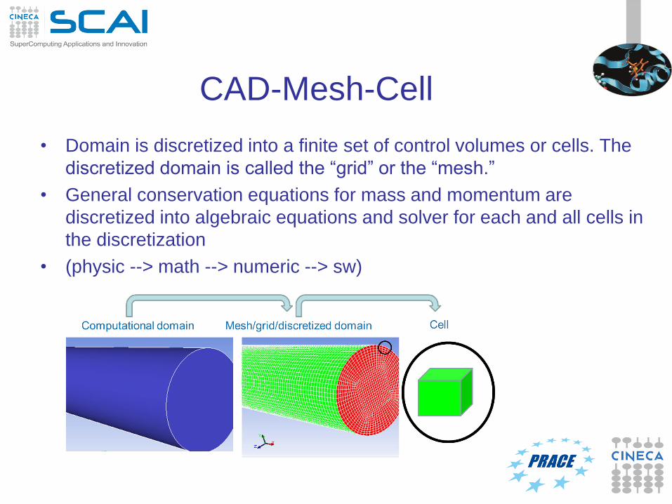
• Domain is discretized into a finite set of control volumes or cells. The

discretized domain is called the “grid” or the “mesh.”

• General conservation equations for mass and momentum are

discretized into algebraic equations and solver for each and all cells in

the discretization

• (physic --> math --> numeric --> sw)

CAD-Mesh-Cell

Finite volume method

The finite-volume method (FVM) is a method for representing and

evaluating partial differential equations in the form of algebraic

equations [LeVeque, 2002; Toro, 1999]. Similar to the finite difference

method or finite element method, values are calculated at discrete

places on a meshed geometry. "Finite volume" refers to the small

volume surrounding each node point on a mesh. In the finite volume

method, volume integrals in a partial differential equation that contain a

divergence term are converted to surface integrals, using the

divergence theorem. These terms are then evaluated as fluxes at the

surfaces of each finite volume. Because the flux entering a given

volume is identical to that leaving the adjacent volume, these methods

are conservative. Another advantage of the finite volume method is that

it is easily formulated to allow for unstructured meshes. The

method is used in many computational fluid dynamics packages.

[Wikipedia]

Finite volume method

• In order to build a CFD model of a physical problem only the portion

of your problem where the fluid is present need to be discretized

(meshed).

• CFD models usually are used to study local phenomena related to a

3D problem so usually only a a certain amount of your physical

domain need to be included in the CFD model (‘nearby’)

• All other parts (solid or ‘far away’) are not of interest and are not

included in the meshing process.

• Example Wind Tunnel Application: the solid object surrounded by

the flowing air is not meshed except for his surface.

• All other surfaces are called numerical boundaries (or just

boundaries) and can be described efficiently within the CFD model

by understanding their main characteristics.

Finite volume method

In order to build a CFD model correctly you must select, accordingly to

your available experimental data or your a-priori knowledge, a coherent

set of boundaries (so that you solve a problem that results in a unique

solution)

Activities involved are:

1. identify the position of the boundaries in your problem

2. recognize what kind of boundary you are dealing with (inlets,

outlets, walls, symmetry, cyclic…)

3. retrieve the information available from your physical proble for

that boundary

Finite volume method

Boundary conditions are a necessary part of the mathematical model.

In fact Navier-Stokes equations and continuity equation in order to be

solved need:

- initial conditions (starting point for the iterative process)

- boundary conditions (define the flow regimen problem)

In order to build a CFD model correctly you must select, accordingly to

your available experimental data or your a-priori knowledge, a coherent

set of boundaries (so that you solve a problem that results in a unique

solution)

Activities involved are:

1. identify the position of the boundaries in your problem

2. recognize what kind of boundary you are dealing with (inlets,

outlets, walls, symmetry, cyclic…)

3. retrieve the information available from your physical problem

for that boundary

Neumann and Dirichlet boundary

conditions

• Dirichlet boundary condition:

Value of velocity at a boundary

u(x) = constant

• Neumann boundary condition:

gradient normal to the boundary of a velocity at the boundary,

nu(x) = constant

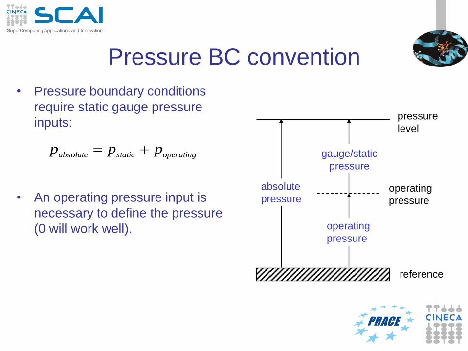
• Pressure boundary conditions

require static gauge pressure

inputs:

• An operating pressure input is

necessary to define the pressure

(0 will work well).

operatingstaticabsoluteppp gauge/static

pressure

operating

pressure

pressure

level

operating

pressure

absolute

pressure

reference

Pressure BC convention

Pressure outlet boundary

• Pressure outlet BC can be used in presence of velocity BC at the inlet

• Usually in a zero-stress condition is applied over multiple exits (if not

known specifically from a-priory knowledge of the problem)

• The geometry is driving the pressure distribution and the flow repartition

• The static pressure is assumed to be constant over the outlet

• A flat profile is selected by default (if not known

specifically from a-priory knowledge of the problem).

• Is very often used as BC to set a known flow-rate

(working condition)

• Thanks to experimental data is possible to obtain spatial

and temporal distribution.

Velocity inlets

• Used to bound the limit between fluid and solid regions in our problem

• Settings at the wall:

– Tangential fluid velocity equal to wall velocity (usually zero))

– Normal velocity component is set to be zero.

Wall boundaries

Symmetry

• When your problem present a symmetry plane in the geometry

and in the flow field this kind of boundary can be used to reduce

computational cost of the CFD model

• General characteristics at the symmetry plane:

– normal velocity equal to zero

– normal gradients of all variables equal to zero

Material properties

• The physiscal property of the fluid must be given.

• For Newtonian Incompressible fluid we have to provide only density and

viscosity.

• Newtonian?

• Incompressible?

Density

• Density is a fluid property and is defined as:

ρ = Mass/Volume

• Usually we consider for water the density value at T=300 K and

P=105 Pa:

ρ = 1060 [Kg/m3 ]

Viscosity

• For viscous flow if the relationship between viscous forces

(tangential component) and velocity gradient is linear then the

fluid is called Newtonian and the slope of the line is a measure

of a fluid property called viscosity (dynamic):

Sy= µ dv/dx

• Also a cinematic viscosity can be defined by:

υ = µ/ρ

Reynolds number

The Reynolds number Re is defined as:

Re = U L /µ

Here:

L is a characteristic length (say D in tubes)

U is the mean velocity over the section(Q/Area)

density and viscosity are: , µ

If Re >> 1 the flow is dominated by inertia.

If Re << 1 the flow is dominated by viscous effects.

Flow classifications

Laminar vs. turbulent flow.

– Laminar flow: fluid particles move in smooth, layered fashion (no

substantial mixing of fluid occurs).

– Turbulent flow: fluid particles move in a chaotic, “tangled” fashion

(significant mixing of fluid occurs).

Steady vs. unsteady flow.

– Steady flow: flow properties at any given point in space are

constant in time, e.g. p = p(x,y,z).

– Unsteady flow: flow properties at any given point in space

change with time, e.g. p = p(x,y,z,t).

Incompressible vs. compressible flow

– Incompressible flow: volume of a given fluid particle does not

change.

• Implies that density is constant everywhere.

• Essentially valid for all liquid flows.

– Compressible flow: volume of a given fluid particle can

change with position.

• Implies that density will vary throughout the flow field.

Single phase vs. multiphase flow

&

homogeneous vs. heterogeneous flow

• Single phase flow: fluid flows without phase change (either liquid or

gas).

• Multiphase flow: multiple phases are present in the flow field (e.g.

liquid-gas, liquid-solid, gas-solid).

• Homogeneous flow: only one fluid material exists in the flow field.

• Heterogeneous flow: multiple fluid/solid materials are present in the

flow field (multi-species flows).

Working hypothesis in CFD for general fluids

• Continuum hypothesis

• Homogenous

• Incompressible (density ρ is constant)

• Isotropic (same behaviour in all directions)

• Newtonian (viscosity (μ and λ) are constant and do not depends

on the shear rate)

In physical models it is very hard to guarantee all these

hypothesis (repeatability and calibration)

Equations of conservation

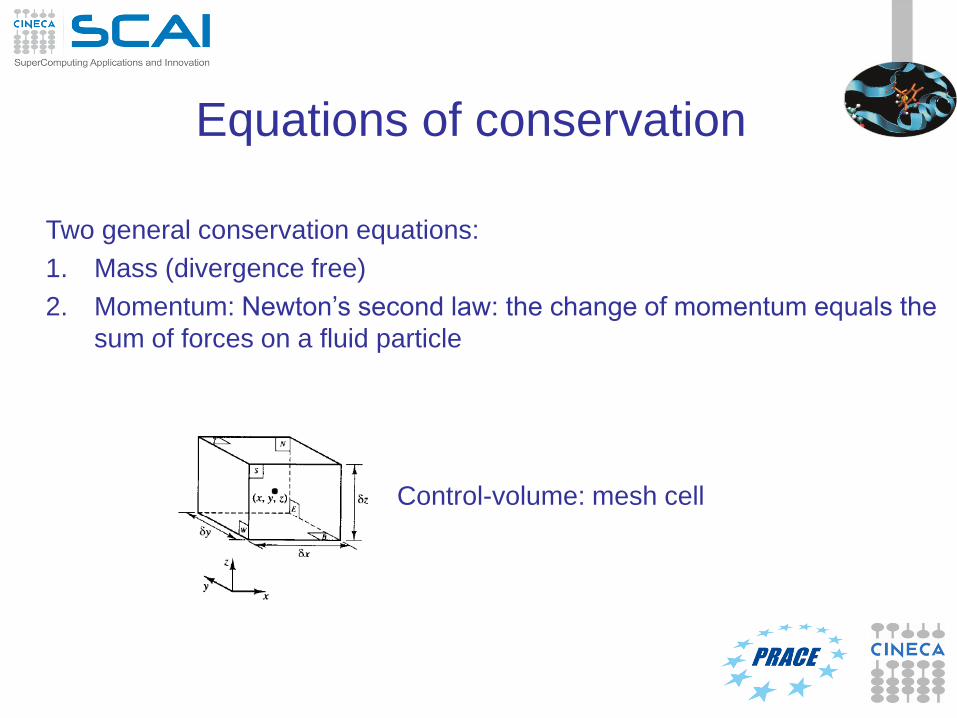
Two general conservation equations:

1. Mass (divergence free)

2. Momentum: Newton’s second law: the change of momentum equals the

sum of forces on a fluid particle

Control-volume: mesh cell

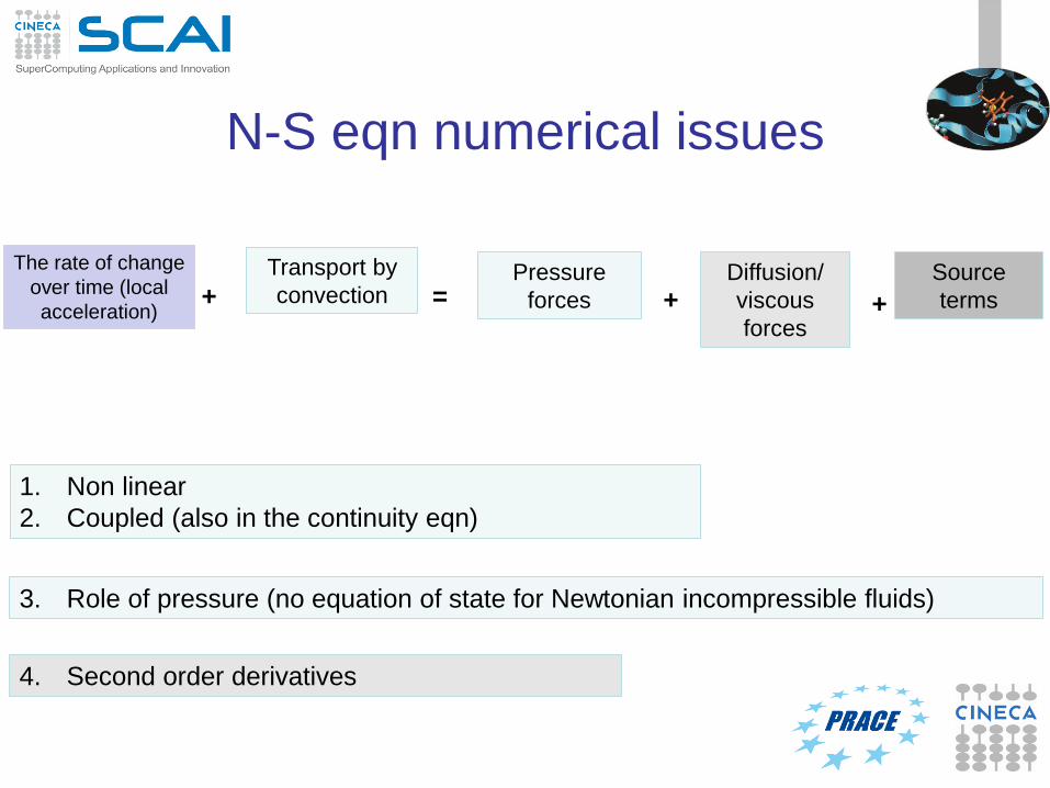
N-S eqn numerical issues

The rate of change

over time (local

acceleration)

Transport by

convection Pressure

forces

Diffusion/

viscous

forces

Source

terms + + + =

1. Non linear

2. Coupled (also in the continuity eqn)

3. Role of pressure (no equation of state for Newtonian incompressible fluids)

4. Second order derivatives

Iterative methods

All the issues abovementioned require numerical methods and

techniques to build accurate and stable tools to integrate such

equations.

Iterative methods

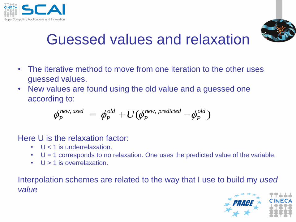
Guessed values and relaxation

• The iterative method to move from one iteration to the other uses

guessed values.

• New values are found using the old value and a guessed one

according to:

Here U is the relaxation factor: • U < 1 is underrelaxation.

• U = 1 corresponds to no relaxation. One uses the predicted value of the variable.

• U > 1 is overrelaxation.

Interpolation schemes are related to the way that I use to build my used

value

, ,( )new used old new predicted old

P P P PU

Conservativeness The conservation of the fluid property must be ensured for each cell and

globally by the algorithm

Local

Global

Boundedness

Iterative methods start from a guessed value and iterate until

convergence criterion is satisfied all over the computational

domain.

In order to converge math says that:

1. Diagonal dominant matrix (from the sys. of eqn.)

2. Coefficients with the same sign (positive)

Physically this means:

1. If you don’t have source terms the values are bounded by

the boundary ones (if the pb is linear).

2. If a property increases its value in one cell then the same

property must increase also in all the cells nearby.

Overshoot and undershoot present for

certain algorithms is related to this

property

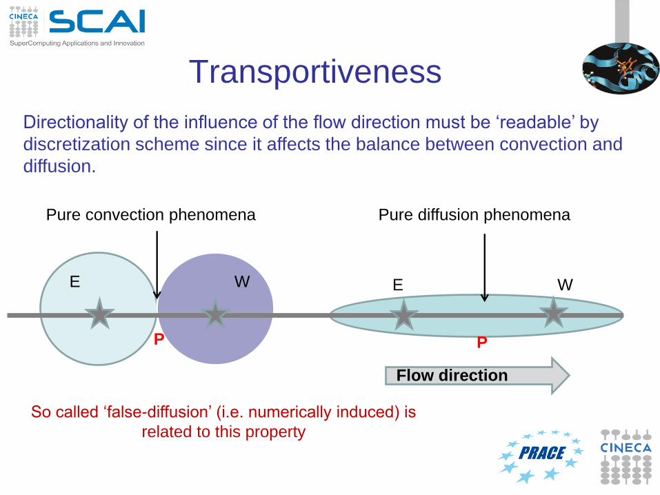
Transportiveness

Directionality of the influence of the flow direction must be ‘readable’ by

discretization scheme since it affects the balance between convection and

diffusion.

Flow direction

Pure convection phenomena Pure diffusion phenomena

P

E W

P

E W

So called ‘false-diffusion’ (i.e. numerically induced) is

related to this property

Pressure - velocity coupling

• For incompressible N-S eqn there is no explicit equation for P.

• P is involved in the momentum equations.

• V must satisfy also continuity equation.

The so-called ‘pressure-velocity’ coupling is an algorithms used to obtain

a valid relationship for the pressure starting from the momentum and the

continuity equation.

The oldest and most popular algorithm is the SIMPLE (Semi-Implicit

Method for Pressure-Linked Equations) by Patankar and Spalding 1972.

What is convergence

Convergence: where do I stop my iterations?

• A flow field solution is considered ‘converged’ when the changes of the properties in the cells from one iteration to another are below a certain fixed value.

• General laws are missing; we have some good rules to understand when we are converged and we can stop to iterate over our solution.

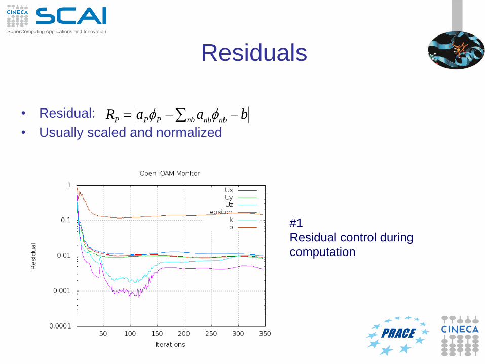
Residuals

• Residual:

• Usually scaled and normalized

baaR nb nbnbPPP

#1

Residual control during

computation

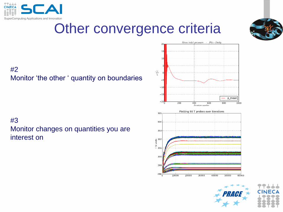
Other convergence criteria

#2

Monitor ‘the other ‘ quantity on boundaries

#3

Monitor changes on quantities you are

interest on

Post-processing

& data visualization

Once the CFD model is ‘at convergence’ the data concerning the flow

field in the discretized domain are available in order to be processed for

quantitative analysis and for visualization.

Scientific visualization over CFD data is one of the most interesting

characteristics of this tool because it allows designers and engineers to

get a better understand of the physical phenomenon and so to improve

the insigth on it.

Once that P and U fields at each point in the domain are available it is

possible to perform further processing and extract no matter wich derived

quantity at any point with an accuracy that is not reachable by common

experimental mesaurements techiniques

Source of errors and uncertainty

• Error: deficiency in a CFD model.

Possible sources of error are:

• Numerical errors (discretization, round-off, convergence)

• Coding errors (bugs)

• User errors

• Uncertainty: deficiency in a CFD model caused by a lack of knowledge.

Possible source of uncertainty are:

• Input data inaccuracies (geometry, BC, material properties)

• Physical model (simplified hypothesis for the fluid behavior)

Verification and Validation (V&V)

Verification: “solving the equation right” (Raoche ‘98).

This process quantify the errors.

Validation: “solving the right equations” (Roache ‘98).

This process quantify the uncertainty.

How should I use it

CFD is a engineering design tool and like any tool can be used with

seccess only were is suited to solve a certain problem and by people

with sufficient knowlegde on how to use the tool.

Wrong tool

Your problem

Right tools