458
HSPICE ® Command Reference Version X-2005.09, September 2005
HSPICE® Command ReferenceVersion X-2005.09, September 2005

ii HSPICE® Command Reference
Copyright Notice and Proprietary InformationCopyright 2005 Synopsys, Inc. All rights reserved. This software and documentation contain confidential and proprietary information that is the property of Synopsys, Inc. The software and documentation are furnished under a license agreement and may be used or copied only in accordance with the terms of the license agreement. No part of the software and documentation may be reproduced, transmitted, or translated, in any form or by any means, electronic, mechanical, manual, optical, or otherwise, without prior written permission of Synopsys, Inc., or as expressly provided by the license agreement.
Right to Copy DocumentationThe license agreement with Synopsys permits licensee to make copies of the documentation for its internal use only. Each copy shall include all copyrights, trademarks, service marks, and proprietary rights notices, if any. Licensee must assign sequential numbers to all copies. These copies shall contain the following legend on the cover page:
“This document is duplicated with the permission of Synopsys, Inc., for the exclusive use of __________________________________________ and its employees. This is copy number __________.”
Destination Control StatementAll technical data contained in this publication is subject to the export control laws of the United States of America. Disclosure to nationals of other countries contrary to United States law is prohibited. It is the reader’s responsibility to determine the applicable regulations and to comply with them.
DisclaimerSYNOPSYS, INC., AND ITS LICENSORS MAKE NO WARRANTY OF ANY KIND, EXPRESS OR IMPLIED, WITH REGARD TO THIS MATERIAL, INCLUDING, BUT NOT LIMITED TO, THE IMPLIED WARRANTIES OF MERCHANTABILITY AND FITNESS FOR A PARTICULAR PURPOSE.
Registered Trademarks (®)Synopsys, AMPS, Arcadia, C Level Design, C2HDL, C2V, C2VHDL, Cadabra, Calaveras Algorithm, CATS, CRITIC, CSim, Design Compiler, DesignPower, DesignWare, EPIC, Formality, HSIM, HSPICE, Hypermodel, iN-Phase, in-Sync, Leda, MAST, Meta, Meta-Software, ModelTools, NanoSim, OpenVera, PathMill, Photolynx, Physical Compiler, PowerMill, PrimeTime, RailMill, RapidScript, Saber, SiVL, SNUG, SolvNet, Superlog, System Compiler, Testify, TetraMAX, TimeMill, TMA, VCS, Vera, and Virtual Stepper are registered trademarks of Synopsys, Inc.
Trademarks (™)Active Parasitics, AFGen, Apollo, Apollo II, Apollo-DPII, Apollo-GA, ApolloGAII, Astro, Astro-Rail, Astro-Xtalk, Aurora, AvanTestchip, AvanWaves, BCView, Behavioral Compiler, BOA, BRT, Cedar, ChipPlanner, Circuit Analysis, Columbia, Columbia-CE, Comet 3D, Cosmos, CosmosEnterprise, CosmosLE, CosmosScope, CosmosSE, Cyclelink, Davinci, DC Expert, DC Expert Plus, DC Professional, DC Ultra, DC Ultra Plus, Design Advisor, Design Analyzer, Design Vision, DesignerHDL, DesignTime, DFM-Workbench, Direct RTL, Direct Silicon Access, Discovery, DW8051, DWPCI, Dynamic-Macromodeling, Dynamic Model Switcher, ECL Compiler, ECO Compiler, EDAnavigator, Encore, Encore PQ, Evaccess, ExpressModel, Floorplan Manager, Formal Model Checker, FoundryModel, FPGA Compiler II, FPGA Express, Frame Compiler, Galaxy, Gatran, HANEX, HDL Advisor, HDL Compiler, Hercules, Hercules-Explorer, Hercules-II, Hierarchical Optimization Technology, High Performance Option, HotPlace, HSIMplus, HSPICE-Link, iN-Tandem, Integrator, Interactive Waveform Viewer, i-Virtual Stepper, Jupiter, Jupiter-DP, JupiterXT, JupiterXT-ASIC, JVXtreme, Liberty, Libra-Passport, Library Compiler, Libra-Visa, Magellan, Mars, Mars-Rail, Mars-Xtalk, Medici, Metacapture, Metacircuit, Metamanager, Metamixsim, Milkyway, ModelSource, Module Compiler, MS-3200, MS-3400, Nova Product Family, Nova-ExploreRTL, Nova-Trans, Nova-VeriLint, Nova-VHDLlint, Optimum Silicon, Orion_ec, Parasitic View, Passport, Planet, Planet-PL, Planet-RTL, Polaris, Polaris-CBS, Polaris-MT, Power Compiler, PowerCODE, PowerGate, ProFPGA, ProGen, Prospector, Protocol Compiler, PSMGen, Raphael, Raphael-NES, RoadRunner, RTL Analyzer, Saturn, ScanBand, Schematic Compiler, Scirocco, Scirocco-i, Shadow Debugger, Silicon Blueprint, Silicon Early Access, SinglePass-SoC, Smart Extraction, SmartLicense, SmartModel Library, Softwire, Source-Level Design, Star, Star-DC, Star-MS, Star-MTB, Star-Power, Star-Rail, Star-RC, Star-RCXT, Star-Sim, Star-SimXT, Star-Time, Star-XP, SWIFT, Taurus, TimeSlice, TimeTracker, Timing Annotator, TopoPlace, TopoRoute, Trace-On-Demand, True-Hspice, TSUPREM-4, TymeWare, VCS Express, VCSi, Venus, Verification Portal, VFormal, VHDL Compiler, VHDL System Simulator, VirSim, and VMC are trademarks of Synopsys, Inc.
Service Marks (SM)MAP-in, SVP Café, and TAP-in are service marks of Synopsys, Inc.
SystemC is a trademark of the Open SystemC Initiative and is used under license.ARM and AMBA are registered trademarks of ARM Limited.All other product or company names may be trademarks of their respective owners. Printed in the U.S.A.
HSPICE® Command Reference, X-2005.09
X-2005.09

Contents
Inside This Manual. . . . . . . . . . . . . . . . . . . . . . . . . . . . . . . . . . . . . . . . . . . . . . xv
The HSPICE Documentation Set. . . . . . . . . . . . . . . . . . . . . . . . . . . . . . . . . . . xvi
Searching Across the HSPICE Documentation Set. . . . . . . . . . . . . . . . . . . . . xvii
Other Related Publications . . . . . . . . . . . . . . . . . . . . . . . . . . . . . . . . . . . . . . . xvii
Conventions . . . . . . . . . . . . . . . . . . . . . . . . . . . . . . . . . . . . . . . . . . . . . . . . . . . xviii
Customer Support . . . . . . . . . . . . . . . . . . . . . . . . . . . . . . . . . . . . . . . . . . . . . . xix
1. Command Categories . . . . . . . . . . . . . . . . . . . . . . . . . . . . . . . . . . . . . . . . . . 1
Alter Blocks . . . . . . . . . . . . . . . . . . . . . . . . . . . . . . . . . . . . . . . . . . . . . . . . . . . 1
Analysis . . . . . . . . . . . . . . . . . . . . . . . . . . . . . . . . . . . . . . . . . . . . . . . . . . . . . . 1
Conditional Block . . . . . . . . . . . . . . . . . . . . . . . . . . . . . . . . . . . . . . . . . . . . . . . 2
Digital Vector . . . . . . . . . . . . . . . . . . . . . . . . . . . . . . . . . . . . . . . . . . . . . . . . . . 2
Encryption . . . . . . . . . . . . . . . . . . . . . . . . . . . . . . . . . . . . . . . . . . . . . . . . . . . . 2
Field Solver . . . . . . . . . . . . . . . . . . . . . . . . . . . . . . . . . . . . . . . . . . . . . . . . . . . 3
Files . . . . . . . . . . . . . . . . . . . . . . . . . . . . . . . . . . . . . . . . . . . . . . . . . . . . . . . . . 3
Input/Output Buffer Information Specification (IBIS) . . . . . . . . . . . . . . . . . . . . 3
Library Management . . . . . . . . . . . . . . . . . . . . . . . . . . . . . . . . . . . . . . . . . . . . 3
Model Definition . . . . . . . . . . . . . . . . . . . . . . . . . . . . . . . . . . . . . . . . . . . . . . . . 4
Node Naming. . . . . . . . . . . . . . . . . . . . . . . . . . . . . . . . . . . . . . . . . . . . . . . . . . 4
Output Porting . . . . . . . . . . . . . . . . . . . . . . . . . . . . . . . . . . . . . . . . . . . . . . . . . 4
Setup . . . . . . . . . . . . . . . . . . . . . . . . . . . . . . . . . . . . . . . . . . . . . . . . . . . . . . . . 4
Simulation Runs. . . . . . . . . . . . . . . . . . . . . . . . . . . . . . . . . . . . . . . . . . . . . . . . 5
Subcircuits . . . . . . . . . . . . . . . . . . . . . . . . . . . . . . . . . . . . . . . . . . . . . . . . . . . . 5
Verilog-A . . . . . . . . . . . . . . . . . . . . . . . . . . . . . . . . . . . . . . . . . . . . . . . . . . . . . 5
HSPICE® Command Reference iiiX-2005.09

Contents
2. Commands in HSPICE Netlists. . . . . . . . . . . . . . . . . . . . . . . . . . . . . . . . . . . 7
.AC . . . . . . . . . . . . . . . . . . . . . . . . . . . . . . . . . . . . . . . . . . . . . . . . . . . . . . . . . . 9
.ALIAS . . . . . . . . . . . . . . . . . . . . . . . . . . . . . . . . . . . . . . . . . . . . . . . . . . . . . . . 14
.ALTER. . . . . . . . . . . . . . . . . . . . . . . . . . . . . . . . . . . . . . . . . . . . . . . . . . . . . . . 16
.BIASCHK . . . . . . . . . . . . . . . . . . . . . . . . . . . . . . . . . . . . . . . . . . . . . . . . . . . . 18
.CONNECT . . . . . . . . . . . . . . . . . . . . . . . . . . . . . . . . . . . . . . . . . . . . . . . . . . . 23
.DATA . . . . . . . . . . . . . . . . . . . . . . . . . . . . . . . . . . . . . . . . . . . . . . . . . . . . . . . . 25
.DC. . . . . . . . . . . . . . . . . . . . . . . . . . . . . . . . . . . . . . . . . . . . . . . . . . . . . . . . . . 32
.DCMATCH . . . . . . . . . . . . . . . . . . . . . . . . . . . . . . . . . . . . . . . . . . . . . . . . . . . 38
.DCVOLT . . . . . . . . . . . . . . . . . . . . . . . . . . . . . . . . . . . . . . . . . . . . . . . . . . . . . 40
.DEL LIB. . . . . . . . . . . . . . . . . . . . . . . . . . . . . . . . . . . . . . . . . . . . . . . . . . . . . . 42
.DISTO . . . . . . . . . . . . . . . . . . . . . . . . . . . . . . . . . . . . . . . . . . . . . . . . . . . . . . . 46
.DOUT . . . . . . . . . . . . . . . . . . . . . . . . . . . . . . . . . . . . . . . . . . . . . . . . . . . . . . . 49
.EBD. . . . . . . . . . . . . . . . . . . . . . . . . . . . . . . . . . . . . . . . . . . . . . . . . . . . . . . . . 52
.ELSE. . . . . . . . . . . . . . . . . . . . . . . . . . . . . . . . . . . . . . . . . . . . . . . . . . . . . . . . 54
.ELSEIF . . . . . . . . . . . . . . . . . . . . . . . . . . . . . . . . . . . . . . . . . . . . . . . . . . . . . . 55
.END . . . . . . . . . . . . . . . . . . . . . . . . . . . . . . . . . . . . . . . . . . . . . . . . . . . . . . . . 56
.ENDDATA . . . . . . . . . . . . . . . . . . . . . . . . . . . . . . . . . . . . . . . . . . . . . . . . . . . . 57
.ENDIF . . . . . . . . . . . . . . . . . . . . . . . . . . . . . . . . . . . . . . . . . . . . . . . . . . . . . . . 58
.ENDL . . . . . . . . . . . . . . . . . . . . . . . . . . . . . . . . . . . . . . . . . . . . . . . . . . . . . . . 59
.ENDS . . . . . . . . . . . . . . . . . . . . . . . . . . . . . . . . . . . . . . . . . . . . . . . . . . . . . . . 60
.EOM . . . . . . . . . . . . . . . . . . . . . . . . . . . . . . . . . . . . . . . . . . . . . . . . . . . . . . . . 61
.FFT . . . . . . . . . . . . . . . . . . . . . . . . . . . . . . . . . . . . . . . . . . . . . . . . . . . . . . . . . 62
.FOUR . . . . . . . . . . . . . . . . . . . . . . . . . . . . . . . . . . . . . . . . . . . . . . . . . . . . . . . 65
.FSOPTIONS . . . . . . . . . . . . . . . . . . . . . . . . . . . . . . . . . . . . . . . . . . . . . . . . . . 66
.GLOBAL . . . . . . . . . . . . . . . . . . . . . . . . . . . . . . . . . . . . . . . . . . . . . . . . . . . . . 68
.GRAPH . . . . . . . . . . . . . . . . . . . . . . . . . . . . . . . . . . . . . . . . . . . . . . . . . . . . . . 69
.HDL. . . . . . . . . . . . . . . . . . . . . . . . . . . . . . . . . . . . . . . . . . . . . . . . . . . . . . . . . 71
.IBIS . . . . . . . . . . . . . . . . . . . . . . . . . . . . . . . . . . . . . . . . . . . . . . . . . . . . . . . . . 72
.IC . . . . . . . . . . . . . . . . . . . . . . . . . . . . . . . . . . . . . . . . . . . . . . . . . . . . . . . . . . 76
iv HSPICE® Command ReferenceX-2005.09
Contents
.ICM . . . . . . . . . . . . . . . . . . . . . . . . . . . . . . . . . . . . . . . . . . . . . . . . . . . . . . . . . 78
.IF. . . . . . . . . . . . . . . . . . . . . . . . . . . . . . . . . . . . . . . . . . . . . . . . . . . . . . . . . . . 79
.INCLUDE . . . . . . . . . . . . . . . . . . . . . . . . . . . . . . . . . . . . . . . . . . . . . . . . . . . . 81
.LAYERSTACK . . . . . . . . . . . . . . . . . . . . . . . . . . . . . . . . . . . . . . . . . . . . . . . . . 82
.LIB . . . . . . . . . . . . . . . . . . . . . . . . . . . . . . . . . . . . . . . . . . . . . . . . . . . . . . . . . 84
.LIN . . . . . . . . . . . . . . . . . . . . . . . . . . . . . . . . . . . . . . . . . . . . . . . . . . . . . . . . . 88
.LOAD . . . . . . . . . . . . . . . . . . . . . . . . . . . . . . . . . . . . . . . . . . . . . . . . . . . . . . . 91
.MACRO. . . . . . . . . . . . . . . . . . . . . . . . . . . . . . . . . . . . . . . . . . . . . . . . . . . . . . 93
.MALIAS. . . . . . . . . . . . . . . . . . . . . . . . . . . . . . . . . . . . . . . . . . . . . . . . . . . . . . 96
.MATERIAL . . . . . . . . . . . . . . . . . . . . . . . . . . . . . . . . . . . . . . . . . . . . . . . . . . . 98
.MEASURE . . . . . . . . . . . . . . . . . . . . . . . . . . . . . . . . . . . . . . . . . . . . . . . . . . . 100
.MEASURE (Rise, Fall, and Delay Measurements) . . . . . . . . . . . . . . . . . . . . . 101
.MEASURE (Average, RMS, and Peak Measurements) . . . . . . . . . . . . . . . . . 105
.MEASURE (FIND and WHEN) . . . . . . . . . . . . . . . . . . . . . . . . . . . . . . . . . . . . 107
.MEASURE (Equation Evaluation/ Arithmetic Expression) . . . . . . . . . . . . . . . 111
.MEASURE (Average, RMS, MIN, MAX, INTEG, and PP). . . . . . . . . . . . . . . . 112
.MEASURE (Integral Function) . . . . . . . . . . . . . . . . . . . . . . . . . . . . . . . . . . . . 115
.MEASURE (Derivative Function) . . . . . . . . . . . . . . . . . . . . . . . . . . . . . . . . . . 116
.MEASURE (Error Function) . . . . . . . . . . . . . . . . . . . . . . . . . . . . . . . . . . . . . . 119
.MEASURE (Pushout Bisection) . . . . . . . . . . . . . . . . . . . . . . . . . . . . . . . . . . . 121
.MODEL . . . . . . . . . . . . . . . . . . . . . . . . . . . . . . . . . . . . . . . . . . . . . . . . . . . . . . 123
.NET. . . . . . . . . . . . . . . . . . . . . . . . . . . . . . . . . . . . . . . . . . . . . . . . . . . . . . . . . 129
.NODESET. . . . . . . . . . . . . . . . . . . . . . . . . . . . . . . . . . . . . . . . . . . . . . . . . . . . 131
.NOISE. . . . . . . . . . . . . . . . . . . . . . . . . . . . . . . . . . . . . . . . . . . . . . . . . . . . . . . 132
.OP. . . . . . . . . . . . . . . . . . . . . . . . . . . . . . . . . . . . . . . . . . . . . . . . . . . . . . . . . . 133
.OPTION . . . . . . . . . . . . . . . . . . . . . . . . . . . . . . . . . . . . . . . . . . . . . . . . . . . . . 135
.PARAM . . . . . . . . . . . . . . . . . . . . . . . . . . . . . . . . . . . . . . . . . . . . . . . . . . . . . . 137
.PAT . . . . . . . . . . . . . . . . . . . . . . . . . . . . . . . . . . . . . . . . . . . . . . . . . . . . . . . . . 141
.PKG . . . . . . . . . . . . . . . . . . . . . . . . . . . . . . . . . . . . . . . . . . . . . . . . . . . . . . . . 143
.PLOT. . . . . . . . . . . . . . . . . . . . . . . . . . . . . . . . . . . . . . . . . . . . . . . . . . . . . . . . 145
.PRINT . . . . . . . . . . . . . . . . . . . . . . . . . . . . . . . . . . . . . . . . . . . . . . . . . . . . . . . 147
HSPICE® Command Reference vX-2005.09

Contents
.PROBE . . . . . . . . . . . . . . . . . . . . . . . . . . . . . . . . . . . . . . . . . . . . . . . . . . . . . . 151
.PROTECT. . . . . . . . . . . . . . . . . . . . . . . . . . . . . . . . . . . . . . . . . . . . . . . . . . . . 153
.PZ . . . . . . . . . . . . . . . . . . . . . . . . . . . . . . . . . . . . . . . . . . . . . . . . . . . . . . . . . . 154
.SAMPLE . . . . . . . . . . . . . . . . . . . . . . . . . . . . . . . . . . . . . . . . . . . . . . . . . . . . . 156
.SAVE. . . . . . . . . . . . . . . . . . . . . . . . . . . . . . . . . . . . . . . . . . . . . . . . . . . . . . . . 157
.SENS . . . . . . . . . . . . . . . . . . . . . . . . . . . . . . . . . . . . . . . . . . . . . . . . . . . . . . . 159
.SHAPE . . . . . . . . . . . . . . . . . . . . . . . . . . . . . . . . . . . . . . . . . . . . . . . . . . . . . . 161
.SHAPE (Defining Rectangles) . . . . . . . . . . . . . . . . . . . . . . . . . . . . . . . . . . . . 162
.SHAPE (Defining Circles) . . . . . . . . . . . . . . . . . . . . . . . . . . . . . . . . . . . . . . . . 163
.SHAPE (Defining Polygons) . . . . . . . . . . . . . . . . . . . . . . . . . . . . . . . . . . . . . . 164
.SHAPE (Defining Strip Polygons) . . . . . . . . . . . . . . . . . . . . . . . . . . . . . . . . . . 166
.STIM . . . . . . . . . . . . . . . . . . . . . . . . . . . . . . . . . . . . . . . . . . . . . . . . . . . . . . . . 167
.SUBCKT . . . . . . . . . . . . . . . . . . . . . . . . . . . . . . . . . . . . . . . . . . . . . . . . . . . . . 172
.TEMP . . . . . . . . . . . . . . . . . . . . . . . . . . . . . . . . . . . . . . . . . . . . . . . . . . . . . . . 175
.TF . . . . . . . . . . . . . . . . . . . . . . . . . . . . . . . . . . . . . . . . . . . . . . . . . . . . . . . . . . 177
.TITLE . . . . . . . . . . . . . . . . . . . . . . . . . . . . . . . . . . . . . . . . . . . . . . . . . . . . . . . 178
.TRAN . . . . . . . . . . . . . . . . . . . . . . . . . . . . . . . . . . . . . . . . . . . . . . . . . . . . . . . 179
.UNPROTECT . . . . . . . . . . . . . . . . . . . . . . . . . . . . . . . . . . . . . . . . . . . . . . . . . 184
.VEC. . . . . . . . . . . . . . . . . . . . . . . . . . . . . . . . . . . . . . . . . . . . . . . . . . . . . . . . . 185
.WIDTH . . . . . . . . . . . . . . . . . . . . . . . . . . . . . . . . . . . . . . . . . . . . . . . . . . . . . . 186
3. Options in HSPICE Netlists. . . . . . . . . . . . . . . . . . . . . . . . . . . . . . . . . . . . . . 187
General Control Options . . . . . . . . . . . . . . . . . . . . . . . . . . . . . . . . . . . . . . . . . 188
CPU Options . . . . . . . . . . . . . . . . . . . . . . . . . . . . . . . . . . . . . . . . . . . . . . . . . . 188
Interface Options . . . . . . . . . . . . . . . . . . . . . . . . . . . . . . . . . . . . . . . . . . . . . . . 188
Analysis Options . . . . . . . . . . . . . . . . . . . . . . . . . . . . . . . . . . . . . . . . . . . . . . . 189
Error Options . . . . . . . . . . . . . . . . . . . . . . . . . . . . . . . . . . . . . . . . . . . . . . . . . . 189
Version Option . . . . . . . . . . . . . . . . . . . . . . . . . . . . . . . . . . . . . . . . . . . . . . . . . 189
Model Analysis Options . . . . . . . . . . . . . . . . . . . . . . . . . . . . . . . . . . . . . . . . . . 189
General Model Analysis Options . . . . . . . . . . . . . . . . . . . . . . . . . . . . . . . 189
MOSFET Model Analysis Options . . . . . . . . . . . . . . . . . . . . . . . . . . . . . . 189
vi HSPICE® Command ReferenceX-2005.09

Contents
Inductor Model Analysis Options . . . . . . . . . . . . . . . . . . . . . . . . . . . . . . . 190
BJT and Diode Model Analysis Options. . . . . . . . . . . . . . . . . . . . . . . . . . 190
DC Operating Point, DC Sweep, and Pole/Zero Options . . . . . . . . . . . . . . . . . 190
DC Accuracy Options. . . . . . . . . . . . . . . . . . . . . . . . . . . . . . . . . . . . . . . . 190
DC Matrix Options . . . . . . . . . . . . . . . . . . . . . . . . . . . . . . . . . . . . . . . . . . 190
DC Pole/Zero I/O Options . . . . . . . . . . . . . . . . . . . . . . . . . . . . . . . . . . . . 190
DC Convergence Options . . . . . . . . . . . . . . . . . . . . . . . . . . . . . . . . . . . . 191
DC Initialization Control Options . . . . . . . . . . . . . . . . . . . . . . . . . . . . . . . 191
Transient and AC Small Signal Analysis Options. . . . . . . . . . . . . . . . . . . . . . . 191
Transient/AC Accuracy Options . . . . . . . . . . . . . . . . . . . . . . . . . . . . . . . . 191
Transient/AC Speed Options . . . . . . . . . . . . . . . . . . . . . . . . . . . . . . . . . . 192
Transient/AC Timestep Options . . . . . . . . . . . . . . . . . . . . . . . . . . . . . . . . 192
Transient/AC Algorithm Options . . . . . . . . . . . . . . . . . . . . . . . . . . . . . . . . 192
.BIASCHK Options . . . . . . . . . . . . . . . . . . . . . . . . . . . . . . . . . . . . . . . . . . 192
Transient Control Options . . . . . . . . . . . . . . . . . . . . . . . . . . . . . . . . . . . . . . . . 193
Transient Control Method Options . . . . . . . . . . . . . . . . . . . . . . . . . . . . . . 193
Transient Control Tolerance Options . . . . . . . . . . . . . . . . . . . . . . . . . . . . 193
Transient Control Limit Options . . . . . . . . . . . . . . . . . . . . . . . . . . . . . . . . 193
Transient Control Matrix Options . . . . . . . . . . . . . . . . . . . . . . . . . . . . . . . 194
Iteration Count Dynamic Timestep Options . . . . . . . . . . . . . . . . . . . . . . . 194
Input/Output Options . . . . . . . . . . . . . . . . . . . . . . . . . . . . . . . . . . . . . . . . . . . . 194
AC Control Options . . . . . . . . . . . . . . . . . . . . . . . . . . . . . . . . . . . . . . . . . . . . . 194
Common Model Interface Options . . . . . . . . . . . . . . . . . . . . . . . . . . . . . . . . . . 194
Verilog-A Options . . . . . . . . . . . . . . . . . . . . . . . . . . . . . . . . . . . . . . . . . . . . . . . 194
.OPTION ABSH . . . . . . . . . . . . . . . . . . . . . . . . . . . . . . . . . . . . . . . . . . . . . . . . 195
.OPTION ABSI . . . . . . . . . . . . . . . . . . . . . . . . . . . . . . . . . . . . . . . . . . . . . . . . . 196
.OPTION ABSMOS . . . . . . . . . . . . . . . . . . . . . . . . . . . . . . . . . . . . . . . . . . . . . 197
.OPTION ABSTOL . . . . . . . . . . . . . . . . . . . . . . . . . . . . . . . . . . . . . . . . . . . . . . 198
.OPTION ABSV . . . . . . . . . . . . . . . . . . . . . . . . . . . . . . . . . . . . . . . . . . . . . . . . 199
.OPTION ABSVAR. . . . . . . . . . . . . . . . . . . . . . . . . . . . . . . . . . . . . . . . . . . . . . 200
.OPTION ABSVDC . . . . . . . . . . . . . . . . . . . . . . . . . . . . . . . . . . . . . . . . . . . . . 201
.OPTION ACCT . . . . . . . . . . . . . . . . . . . . . . . . . . . . . . . . . . . . . . . . . . . . . . . . 202
.OPTION ACCURATE . . . . . . . . . . . . . . . . . . . . . . . . . . . . . . . . . . . . . . . . . . . 203
.OPTION ACOUT. . . . . . . . . . . . . . . . . . . . . . . . . . . . . . . . . . . . . . . . . . . . . . . 204
HSPICE® Command Reference viiX-2005.09
Contents
.OPTION ALT999 or ALT9999 . . . . . . . . . . . . . . . . . . . . . . . . . . . . . . . . . . . . . 205
OPTION ALTCC. . . . . . . . . . . . . . . . . . . . . . . . . . . . . . . . . . . . . . . . . . . . . . . . 206
.OPTION ALTCHK . . . . . . . . . . . . . . . . . . . . . . . . . . . . . . . . . . . . . . . . . . . . . . 207
.OPTION ARTIST . . . . . . . . . . . . . . . . . . . . . . . . . . . . . . . . . . . . . . . . . . . . . . 208
.OPTION ASPEC. . . . . . . . . . . . . . . . . . . . . . . . . . . . . . . . . . . . . . . . . . . . . . . 209
.OPTION AUTOSTOP . . . . . . . . . . . . . . . . . . . . . . . . . . . . . . . . . . . . . . . . . . . 210
.OPTION BADCHR . . . . . . . . . . . . . . . . . . . . . . . . . . . . . . . . . . . . . . . . . . . . . 211
.OPTION BEEP . . . . . . . . . . . . . . . . . . . . . . . . . . . . . . . . . . . . . . . . . . . . . . . . 212
.OPTION BIASFILE . . . . . . . . . . . . . . . . . . . . . . . . . . . . . . . . . . . . . . . . . . . . . 213
.OPTION BIAWARN. . . . . . . . . . . . . . . . . . . . . . . . . . . . . . . . . . . . . . . . . . . . . 214
.OPTION BINPRINT . . . . . . . . . . . . . . . . . . . . . . . . . . . . . . . . . . . . . . . . . . . . 215
.OPTION BKPSIZ . . . . . . . . . . . . . . . . . . . . . . . . . . . . . . . . . . . . . . . . . . . . . . 216
.OPTION BRIEF. . . . . . . . . . . . . . . . . . . . . . . . . . . . . . . . . . . . . . . . . . . . . . . . 217
.OPTION BYPASS . . . . . . . . . . . . . . . . . . . . . . . . . . . . . . . . . . . . . . . . . . . . . . 218
.OPTION BYTOL . . . . . . . . . . . . . . . . . . . . . . . . . . . . . . . . . . . . . . . . . . . . . . . 219
.OPTION CAPTAB . . . . . . . . . . . . . . . . . . . . . . . . . . . . . . . . . . . . . . . . . . . . . . 220
.OPTION CDS . . . . . . . . . . . . . . . . . . . . . . . . . . . . . . . . . . . . . . . . . . . . . . . . . 221
.OPTION CHGTOL . . . . . . . . . . . . . . . . . . . . . . . . . . . . . . . . . . . . . . . . . . . . . 222
.OPTION CMIFLAG . . . . . . . . . . . . . . . . . . . . . . . . . . . . . . . . . . . . . . . . . . . . . 223
.OPTION CO . . . . . . . . . . . . . . . . . . . . . . . . . . . . . . . . . . . . . . . . . . . . . . . . . . 224
.OPTION CONVERGE. . . . . . . . . . . . . . . . . . . . . . . . . . . . . . . . . . . . . . . . . . . 225
.OPTION CPTIME . . . . . . . . . . . . . . . . . . . . . . . . . . . . . . . . . . . . . . . . . . . . . . 226
.OPTION CSDF . . . . . . . . . . . . . . . . . . . . . . . . . . . . . . . . . . . . . . . . . . . . . . . . 227
.OPTION CSHDC . . . . . . . . . . . . . . . . . . . . . . . . . . . . . . . . . . . . . . . . . . . . . . 228
.OPTION CSHUNT . . . . . . . . . . . . . . . . . . . . . . . . . . . . . . . . . . . . . . . . . . . . . 229
.OPTION CUSTCMI. . . . . . . . . . . . . . . . . . . . . . . . . . . . . . . . . . . . . . . . . . . . . 230
.OPTION CVTOL . . . . . . . . . . . . . . . . . . . . . . . . . . . . . . . . . . . . . . . . . . . . . . . 231
.OPTION D_IBIS . . . . . . . . . . . . . . . . . . . . . . . . . . . . . . . . . . . . . . . . . . . . . . . 232
.OPTION DCAP . . . . . . . . . . . . . . . . . . . . . . . . . . . . . . . . . . . . . . . . . . . . . . . . 233
.OPTION DCCAP. . . . . . . . . . . . . . . . . . . . . . . . . . . . . . . . . . . . . . . . . . . . . . . 234
.OPTION DCFOR . . . . . . . . . . . . . . . . . . . . . . . . . . . . . . . . . . . . . . . . . . . . . . 235
viii HSPICE® Command ReferenceX-2005.09
Contents
.OPTION DCHOLD . . . . . . . . . . . . . . . . . . . . . . . . . . . . . . . . . . . . . . . . . . . . . 236
.OPTION DCIC . . . . . . . . . . . . . . . . . . . . . . . . . . . . . . . . . . . . . . . . . . . . . . . . 237
.OPTION DCON. . . . . . . . . . . . . . . . . . . . . . . . . . . . . . . . . . . . . . . . . . . . . . . . 238
.OPTION DCSTEP. . . . . . . . . . . . . . . . . . . . . . . . . . . . . . . . . . . . . . . . . . . . . . 239
.OPTION DCTRAN . . . . . . . . . . . . . . . . . . . . . . . . . . . . . . . . . . . . . . . . . . . . . 240
.OPTION DEFAD . . . . . . . . . . . . . . . . . . . . . . . . . . . . . . . . . . . . . . . . . . . . . . . 241
.OPTION DEFAS . . . . . . . . . . . . . . . . . . . . . . . . . . . . . . . . . . . . . . . . . . . . . . . 242
.OPTION DEFL . . . . . . . . . . . . . . . . . . . . . . . . . . . . . . . . . . . . . . . . . . . . . . . . 243
.OPTION DEFNRD . . . . . . . . . . . . . . . . . . . . . . . . . . . . . . . . . . . . . . . . . . . . . 244
.OPTION DEFNRS . . . . . . . . . . . . . . . . . . . . . . . . . . . . . . . . . . . . . . . . . . . . . 245
.OPTION DEFPD. . . . . . . . . . . . . . . . . . . . . . . . . . . . . . . . . . . . . . . . . . . . . . . 246
.OPTION DEFPS . . . . . . . . . . . . . . . . . . . . . . . . . . . . . . . . . . . . . . . . . . . . . . . 247
.OPTION DEFW. . . . . . . . . . . . . . . . . . . . . . . . . . . . . . . . . . . . . . . . . . . . . . . . 248
.OPTION DELMAX . . . . . . . . . . . . . . . . . . . . . . . . . . . . . . . . . . . . . . . . . . . . . 249
.OPTION DI . . . . . . . . . . . . . . . . . . . . . . . . . . . . . . . . . . . . . . . . . . . . . . . . . . . 250
.OPTION DIAGNOSTIC. . . . . . . . . . . . . . . . . . . . . . . . . . . . . . . . . . . . . . . . . . 251
.OPTION DLENCSDF . . . . . . . . . . . . . . . . . . . . . . . . . . . . . . . . . . . . . . . . . . . 252
.OPTION DV . . . . . . . . . . . . . . . . . . . . . . . . . . . . . . . . . . . . . . . . . . . . . . . . . . 253
.OPTION DVDT . . . . . . . . . . . . . . . . . . . . . . . . . . . . . . . . . . . . . . . . . . . . . . . . 254
.OPTION DVTR . . . . . . . . . . . . . . . . . . . . . . . . . . . . . . . . . . . . . . . . . . . . . . . . 255
.OPTION EPSMIN . . . . . . . . . . . . . . . . . . . . . . . . . . . . . . . . . . . . . . . . . . . . . . 256
.OPTION EXPLI . . . . . . . . . . . . . . . . . . . . . . . . . . . . . . . . . . . . . . . . . . . . . . . . 257
.OPTION EXPMAX . . . . . . . . . . . . . . . . . . . . . . . . . . . . . . . . . . . . . . . . . . . . . 258
.OPTION FAST . . . . . . . . . . . . . . . . . . . . . . . . . . . . . . . . . . . . . . . . . . . . . . . . 259
.OPTION FFTOUT . . . . . . . . . . . . . . . . . . . . . . . . . . . . . . . . . . . . . . . . . . . . . . 260
.OPTION FS. . . . . . . . . . . . . . . . . . . . . . . . . . . . . . . . . . . . . . . . . . . . . . . . . . . 261
.OPTION FT. . . . . . . . . . . . . . . . . . . . . . . . . . . . . . . . . . . . . . . . . . . . . . . . . . . 262
.OPTION GDCPATH . . . . . . . . . . . . . . . . . . . . . . . . . . . . . . . . . . . . . . . . . . . . 263
.OPTION GENK. . . . . . . . . . . . . . . . . . . . . . . . . . . . . . . . . . . . . . . . . . . . . . . . 264
.OPTION GMAX. . . . . . . . . . . . . . . . . . . . . . . . . . . . . . . . . . . . . . . . . . . . . . . . 265
.OPTION GMIN . . . . . . . . . . . . . . . . . . . . . . . . . . . . . . . . . . . . . . . . . . . . . . . . 266
HSPICE® Command Reference ixX-2005.09

Contents
.OPTION GMINDC. . . . . . . . . . . . . . . . . . . . . . . . . . . . . . . . . . . . . . . . . . . . . . 267
.OPTION GRAMP . . . . . . . . . . . . . . . . . . . . . . . . . . . . . . . . . . . . . . . . . . . . . . 268
.OPTION GSHDC . . . . . . . . . . . . . . . . . . . . . . . . . . . . . . . . . . . . . . . . . . . . . . 269
.OPTION GSHUNT . . . . . . . . . . . . . . . . . . . . . . . . . . . . . . . . . . . . . . . . . . . . . 270
.OPTION H9007. . . . . . . . . . . . . . . . . . . . . . . . . . . . . . . . . . . . . . . . . . . . . . . . 271
.OPTION HIER_SCALE. . . . . . . . . . . . . . . . . . . . . . . . . . . . . . . . . . . . . . . . . . 272
.OPTION ICSWEEP. . . . . . . . . . . . . . . . . . . . . . . . . . . . . . . . . . . . . . . . . . . . . 273
.OPTION IMAX . . . . . . . . . . . . . . . . . . . . . . . . . . . . . . . . . . . . . . . . . . . . . . . . 274
.OPTION IMIN . . . . . . . . . . . . . . . . . . . . . . . . . . . . . . . . . . . . . . . . . . . . . . . . . 275
.OPTION INGOLD . . . . . . . . . . . . . . . . . . . . . . . . . . . . . . . . . . . . . . . . . . . . . . 276
.OPTION INTERP . . . . . . . . . . . . . . . . . . . . . . . . . . . . . . . . . . . . . . . . . . . . . . 277
.OPTION ITL1 . . . . . . . . . . . . . . . . . . . . . . . . . . . . . . . . . . . . . . . . . . . . . . . . . 278
.OPTION ITL2 . . . . . . . . . . . . . . . . . . . . . . . . . . . . . . . . . . . . . . . . . . . . . . . . . 279
.OPTION ITL3 . . . . . . . . . . . . . . . . . . . . . . . . . . . . . . . . . . . . . . . . . . . . . . . . . 280
.OPTION ITL4 . . . . . . . . . . . . . . . . . . . . . . . . . . . . . . . . . . . . . . . . . . . . . . . . . 281
.OPTION ITL5 . . . . . . . . . . . . . . . . . . . . . . . . . . . . . . . . . . . . . . . . . . . . . . . . . 282
.OPTION ITLPTRAN . . . . . . . . . . . . . . . . . . . . . . . . . . . . . . . . . . . . . . . . . . . . 283
.OPTION ITLPZ . . . . . . . . . . . . . . . . . . . . . . . . . . . . . . . . . . . . . . . . . . . . . . . . 284
.OPTION ITRPRT . . . . . . . . . . . . . . . . . . . . . . . . . . . . . . . . . . . . . . . . . . . . . . 285
.OPTION KCLTEST . . . . . . . . . . . . . . . . . . . . . . . . . . . . . . . . . . . . . . . . . . . . . 286
.OPTION KLIM. . . . . . . . . . . . . . . . . . . . . . . . . . . . . . . . . . . . . . . . . . . . . . . . . 287
.OPTION LENNAM . . . . . . . . . . . . . . . . . . . . . . . . . . . . . . . . . . . . . . . . . . . . . 288
.OPTION LIMPTS . . . . . . . . . . . . . . . . . . . . . . . . . . . . . . . . . . . . . . . . . . . . . . 289
.OPTION LIMTIM. . . . . . . . . . . . . . . . . . . . . . . . . . . . . . . . . . . . . . . . . . . . . . . 290
.OPTION LIST . . . . . . . . . . . . . . . . . . . . . . . . . . . . . . . . . . . . . . . . . . . . . . . . . 291
.OPTION LVLTIM . . . . . . . . . . . . . . . . . . . . . . . . . . . . . . . . . . . . . . . . . . . . . . . 292
.OPTION MAXAMP . . . . . . . . . . . . . . . . . . . . . . . . . . . . . . . . . . . . . . . . . . . . . 293
.OPTION MAXORD . . . . . . . . . . . . . . . . . . . . . . . . . . . . . . . . . . . . . . . . . . . . . 294
.OPTION MBYPASS . . . . . . . . . . . . . . . . . . . . . . . . . . . . . . . . . . . . . . . . . . . . 295
.OPTION MCBRIEF. . . . . . . . . . . . . . . . . . . . . . . . . . . . . . . . . . . . . . . . . . . . . 296
.OPTION MEASDGT . . . . . . . . . . . . . . . . . . . . . . . . . . . . . . . . . . . . . . . . . . . . 297
x HSPICE® Command ReferenceX-2005.09

Contents
.OPTION MEASFAIL . . . . . . . . . . . . . . . . . . . . . . . . . . . . . . . . . . . . . . . . . . . . 298
.OPTION MEASFILE . . . . . . . . . . . . . . . . . . . . . . . . . . . . . . . . . . . . . . . . . . . . 299
.OPTION MEASSORT . . . . . . . . . . . . . . . . . . . . . . . . . . . . . . . . . . . . . . . . . . . 300
.OPTION MEASOUT . . . . . . . . . . . . . . . . . . . . . . . . . . . . . . . . . . . . . . . . . . . . 301
.OPTION MENTOR . . . . . . . . . . . . . . . . . . . . . . . . . . . . . . . . . . . . . . . . . . . . . 302
.OPTION METHOD . . . . . . . . . . . . . . . . . . . . . . . . . . . . . . . . . . . . . . . . . . . . . 303
.OPTION MODMONTE . . . . . . . . . . . . . . . . . . . . . . . . . . . . . . . . . . . . . . . . . . 304
.OPTION MODSRH . . . . . . . . . . . . . . . . . . . . . . . . . . . . . . . . . . . . . . . . . . . . . 305
.OPTION MONTECON . . . . . . . . . . . . . . . . . . . . . . . . . . . . . . . . . . . . . . . . . . 306
.OPTION MU . . . . . . . . . . . . . . . . . . . . . . . . . . . . . . . . . . . . . . . . . . . . . . . . . . 307
.OPTION NEWTOL . . . . . . . . . . . . . . . . . . . . . . . . . . . . . . . . . . . . . . . . . . . . . 308
.OPTION NODE. . . . . . . . . . . . . . . . . . . . . . . . . . . . . . . . . . . . . . . . . . . . . . . . 309
.OPTION NOELCK . . . . . . . . . . . . . . . . . . . . . . . . . . . . . . . . . . . . . . . . . . . . . 310
.OPTION NOISEMINFREQ . . . . . . . . . . . . . . . . . . . . . . . . . . . . . . . . . . . . . . . 311
.OPTION NOMOD . . . . . . . . . . . . . . . . . . . . . . . . . . . . . . . . . . . . . . . . . . . . . . 312
.OPTION NOPAGE . . . . . . . . . . . . . . . . . . . . . . . . . . . . . . . . . . . . . . . . . . . . . 313
.OPTION NOPIV . . . . . . . . . . . . . . . . . . . . . . . . . . . . . . . . . . . . . . . . . . . . . . . 314
.OPTION NOTOP. . . . . . . . . . . . . . . . . . . . . . . . . . . . . . . . . . . . . . . . . . . . . . . 315
.OPTION NOWARN . . . . . . . . . . . . . . . . . . . . . . . . . . . . . . . . . . . . . . . . . . . . . 316
.OPTION NUMDGT . . . . . . . . . . . . . . . . . . . . . . . . . . . . . . . . . . . . . . . . . . . . . 317
.OPTION NXX . . . . . . . . . . . . . . . . . . . . . . . . . . . . . . . . . . . . . . . . . . . . . . . . . 318
.OPTION OFF . . . . . . . . . . . . . . . . . . . . . . . . . . . . . . . . . . . . . . . . . . . . . . . . . 319
.OPTION OPFILE . . . . . . . . . . . . . . . . . . . . . . . . . . . . . . . . . . . . . . . . . . . . . . 320
.OPTION OPTLST . . . . . . . . . . . . . . . . . . . . . . . . . . . . . . . . . . . . . . . . . . . . . . 321
.OPTION OPTS . . . . . . . . . . . . . . . . . . . . . . . . . . . . . . . . . . . . . . . . . . . . . . . . 322
.OPTION PARHIER . . . . . . . . . . . . . . . . . . . . . . . . . . . . . . . . . . . . . . . . . . . . . 323
.OPTION PATHNUM . . . . . . . . . . . . . . . . . . . . . . . . . . . . . . . . . . . . . . . . . . . . 324
.OPTION PIVOT. . . . . . . . . . . . . . . . . . . . . . . . . . . . . . . . . . . . . . . . . . . . . . . . 325
.OPTION PIVREF . . . . . . . . . . . . . . . . . . . . . . . . . . . . . . . . . . . . . . . . . . . . . . 327
.OPTION PIVREL . . . . . . . . . . . . . . . . . . . . . . . . . . . . . . . . . . . . . . . . . . . . . . 328
.OPTION PIVTOL . . . . . . . . . . . . . . . . . . . . . . . . . . . . . . . . . . . . . . . . . . . . . . 329
HSPICE® Command Reference xiX-2005.09

Contents
.OPTION PLIM. . . . . . . . . . . . . . . . . . . . . . . . . . . . . . . . . . . . . . . . . . . . . . . . . 330
.OPTION POST . . . . . . . . . . . . . . . . . . . . . . . . . . . . . . . . . . . . . . . . . . . . . . . . 331
.OPTION POSTLVL . . . . . . . . . . . . . . . . . . . . . . . . . . . . . . . . . . . . . . . . . . . . . 332
.OPTION POST_VERSION . . . . . . . . . . . . . . . . . . . . . . . . . . . . . . . . . . . . . . . 333
.OPTION POSTTOP . . . . . . . . . . . . . . . . . . . . . . . . . . . . . . . . . . . . . . . . . . . . 334
.OPTION PROBE. . . . . . . . . . . . . . . . . . . . . . . . . . . . . . . . . . . . . . . . . . . . . . . 335
.OPTION PSF . . . . . . . . . . . . . . . . . . . . . . . . . . . . . . . . . . . . . . . . . . . . . . . . . 336
.OPTION PURETP. . . . . . . . . . . . . . . . . . . . . . . . . . . . . . . . . . . . . . . . . . . . . . 337
.OPTION PUTMEAS . . . . . . . . . . . . . . . . . . . . . . . . . . . . . . . . . . . . . . . . . . . . 338
.OPTION RELH . . . . . . . . . . . . . . . . . . . . . . . . . . . . . . . . . . . . . . . . . . . . . . . . 339
.OPTION RELI . . . . . . . . . . . . . . . . . . . . . . . . . . . . . . . . . . . . . . . . . . . . . . . . . 340
.OPTION RELMOS . . . . . . . . . . . . . . . . . . . . . . . . . . . . . . . . . . . . . . . . . . . . . 341
.OPTION RELQ . . . . . . . . . . . . . . . . . . . . . . . . . . . . . . . . . . . . . . . . . . . . . . . . 342
.OPTION RELTOL . . . . . . . . . . . . . . . . . . . . . . . . . . . . . . . . . . . . . . . . . . . . . . 343
.OPTION RELV . . . . . . . . . . . . . . . . . . . . . . . . . . . . . . . . . . . . . . . . . . . . . . . . 344
.OPTION RELVAR . . . . . . . . . . . . . . . . . . . . . . . . . . . . . . . . . . . . . . . . . . . . . . 345
.OPTION RELVDC. . . . . . . . . . . . . . . . . . . . . . . . . . . . . . . . . . . . . . . . . . . . . . 346
.OPTION RESMIN . . . . . . . . . . . . . . . . . . . . . . . . . . . . . . . . . . . . . . . . . . . . . . 347
.OPTION RISETIME . . . . . . . . . . . . . . . . . . . . . . . . . . . . . . . . . . . . . . . . . . . . 348
.OPTION RMAX. . . . . . . . . . . . . . . . . . . . . . . . . . . . . . . . . . . . . . . . . . . . . . . . 349
.OPTION RMIN . . . . . . . . . . . . . . . . . . . . . . . . . . . . . . . . . . . . . . . . . . . . . . . . 350
.OPTION RUNLVL . . . . . . . . . . . . . . . . . . . . . . . . . . . . . . . . . . . . . . . . . . . . . . 351
.OPTION SCALE . . . . . . . . . . . . . . . . . . . . . . . . . . . . . . . . . . . . . . . . . . . . . . . 353
.OPTION SCALM. . . . . . . . . . . . . . . . . . . . . . . . . . . . . . . . . . . . . . . . . . . . . . . 354
.OPTION SDA . . . . . . . . . . . . . . . . . . . . . . . . . . . . . . . . . . . . . . . . . . . . . . . . . 355
.OPTION SEARCH . . . . . . . . . . . . . . . . . . . . . . . . . . . . . . . . . . . . . . . . . . . . . 356
.OPTION SEED . . . . . . . . . . . . . . . . . . . . . . . . . . . . . . . . . . . . . . . . . . . . . . . . 357
.OPTION SLOPETOL . . . . . . . . . . . . . . . . . . . . . . . . . . . . . . . . . . . . . . . . . . . 358
.OPTION SPARSE. . . . . . . . . . . . . . . . . . . . . . . . . . . . . . . . . . . . . . . . . . . . . . 359
.OPTION SPICE . . . . . . . . . . . . . . . . . . . . . . . . . . . . . . . . . . . . . . . . . . . . . . . 360
.OPTION SPMODEL . . . . . . . . . . . . . . . . . . . . . . . . . . . . . . . . . . . . . . . . . . . . 361
xii HSPICE® Command ReferenceX-2005.09

Contents
.OPTION STATFL. . . . . . . . . . . . . . . . . . . . . . . . . . . . . . . . . . . . . . . . . . . . . . . 362
.OPTION SYMB. . . . . . . . . . . . . . . . . . . . . . . . . . . . . . . . . . . . . . . . . . . . . . . . 363
.OPTION TIMERES . . . . . . . . . . . . . . . . . . . . . . . . . . . . . . . . . . . . . . . . . . . . . 364
.OPTION TNOM. . . . . . . . . . . . . . . . . . . . . . . . . . . . . . . . . . . . . . . . . . . . . . . . 365
.OPTION TRCON . . . . . . . . . . . . . . . . . . . . . . . . . . . . . . . . . . . . . . . . . . . . . . 366
.OPTION TRTOL . . . . . . . . . . . . . . . . . . . . . . . . . . . . . . . . . . . . . . . . . . . . . . . 368
.OPTION UNWRAP . . . . . . . . . . . . . . . . . . . . . . . . . . . . . . . . . . . . . . . . . . . . . 369
.OPTION VAMODEL . . . . . . . . . . . . . . . . . . . . . . . . . . . . . . . . . . . . . . . . . . . . 370
.OPTION VERIFY . . . . . . . . . . . . . . . . . . . . . . . . . . . . . . . . . . . . . . . . . . . . . . 371
.OPTION VFLOOR . . . . . . . . . . . . . . . . . . . . . . . . . . . . . . . . . . . . . . . . . . . . . 372
.OPTION VNTOL . . . . . . . . . . . . . . . . . . . . . . . . . . . . . . . . . . . . . . . . . . . . . . . 373
.OPTION WACC . . . . . . . . . . . . . . . . . . . . . . . . . . . . . . . . . . . . . . . . . . . . . . . 374
.OPTION WNFLAG . . . . . . . . . . . . . . . . . . . . . . . . . . . . . . . . . . . . . . . . . . . . . 375
.OPTION WARNLIMIT . . . . . . . . . . . . . . . . . . . . . . . . . . . . . . . . . . . . . . . . . . . 376
.OPTION WL . . . . . . . . . . . . . . . . . . . . . . . . . . . . . . . . . . . . . . . . . . . . . . . . . . 377
.OPTION XDTEMP . . . . . . . . . . . . . . . . . . . . . . . . . . . . . . . . . . . . . . . . . . . . . 378
.OPTION ZUKEN. . . . . . . . . . . . . . . . . . . . . . . . . . . . . . . . . . . . . . . . . . . . . . . 379
4. Commands in Digital Vector Files . . . . . . . . . . . . . . . . . . . . . . . . . . . . . . . . 393
ENABLE. . . . . . . . . . . . . . . . . . . . . . . . . . . . . . . . . . . . . . . . . . . . . . . . . . . . . . 394
IDELAY . . . . . . . . . . . . . . . . . . . . . . . . . . . . . . . . . . . . . . . . . . . . . . . . . . . . . . 395
IO . . . . . . . . . . . . . . . . . . . . . . . . . . . . . . . . . . . . . . . . . . . . . . . . . . . . . . . . . . . 397
ODELAY. . . . . . . . . . . . . . . . . . . . . . . . . . . . . . . . . . . . . . . . . . . . . . . . . . . . . . 398
OUT or OUTZ . . . . . . . . . . . . . . . . . . . . . . . . . . . . . . . . . . . . . . . . . . . . . . . . . 400
PERIOD . . . . . . . . . . . . . . . . . . . . . . . . . . . . . . . . . . . . . . . . . . . . . . . . . . . . . . 401
RADIX . . . . . . . . . . . . . . . . . . . . . . . . . . . . . . . . . . . . . . . . . . . . . . . . . . . . . . . 402
SLOPE. . . . . . . . . . . . . . . . . . . . . . . . . . . . . . . . . . . . . . . . . . . . . . . . . . . . . . . 403
TDELAY . . . . . . . . . . . . . . . . . . . . . . . . . . . . . . . . . . . . . . . . . . . . . . . . . . . . . . 404
TFALL . . . . . . . . . . . . . . . . . . . . . . . . . . . . . . . . . . . . . . . . . . . . . . . . . . . . . . . 406
TRISE . . . . . . . . . . . . . . . . . . . . . . . . . . . . . . . . . . . . . . . . . . . . . . . . . . . . . . . 407
TRIZ. . . . . . . . . . . . . . . . . . . . . . . . . . . . . . . . . . . . . . . . . . . . . . . . . . . . . . . . . 409
HSPICE® Command Reference xiiiX-2005.09

Contents
TSKIP. . . . . . . . . . . . . . . . . . . . . . . . . . . . . . . . . . . . . . . . . . . . . . . . . . . . . . . . 410
TUNIT . . . . . . . . . . . . . . . . . . . . . . . . . . . . . . . . . . . . . . . . . . . . . . . . . . . . . . . 411
VIH. . . . . . . . . . . . . . . . . . . . . . . . . . . . . . . . . . . . . . . . . . . . . . . . . . . . . . . . . . 412
VIL . . . . . . . . . . . . . . . . . . . . . . . . . . . . . . . . . . . . . . . . . . . . . . . . . . . . . . . . . . 413
VNAME . . . . . . . . . . . . . . . . . . . . . . . . . . . . . . . . . . . . . . . . . . . . . . . . . . . . . . 414
VOH . . . . . . . . . . . . . . . . . . . . . . . . . . . . . . . . . . . . . . . . . . . . . . . . . . . . . . . . . 416
VOL . . . . . . . . . . . . . . . . . . . . . . . . . . . . . . . . . . . . . . . . . . . . . . . . . . . . . . . . . 418
VREF . . . . . . . . . . . . . . . . . . . . . . . . . . . . . . . . . . . . . . . . . . . . . . . . . . . . . . . . 420
VTH . . . . . . . . . . . . . . . . . . . . . . . . . . . . . . . . . . . . . . . . . . . . . . . . . . . . . . . . . 421
Index . . . . . . . . . . . . . . . . . . . . . . . . . . . . . . . . . . . . . . . . . . . . . . . . . . . . . . . . . . . . 423
xiv HSPICE® Command ReferenceX-2005.09

About This Manual
This manual describes the individual HSPICE commands you can use to simulate and analyze your circuit designs.
Inside This Manual
This manual contains the chapters described below. For descriptions of the other manuals in the HSPICE documentation set, see the next section, The HSPICE Documentation Set.
Chapter Description
Chapter 1, Command Categories
Lists all commands you can use in HSPICE, arranged by task.
Chapter 2, Commands in HSPICE Netlists
Contains an alphabetical listing of all commands you can use in an HSPICE netlist.
Chapter 3, Options in HSPICE Netlists
Describes the simulation options you can set using various forms of the .OPTION command.
Chapter 4, Commands in Digital Vector Files
Contains an alphabetical listing of the commands you can use in an digital vector file.
HSPICE® Command Reference xvX-2005.09

About This ManualThe HSPICE Documentation Set
The HSPICE Documentation Set
This manual is a part of the HSPICE documentation set, which includes the following manuals:
Manual Description
HSPICE Simulation and Analysis User Guide
Describes how to use HSPICE to simulate and analyze your circuit designs. This is the main HSPICE user guide.
HSPICE Signal Integrity Guide
Describes how to use HSPICE to maintain signal integrity in your chip design.
HSPICE Applications Manual
Provides application examples and additional HSPICE user information.
HSPICE Command Reference
Provides reference information for HSPICE commands.
HPSPICE Elements and Device Models Manual
Describes standard models you can use when simulating your circuit designs in HSPICE, including passive devices, diodes, JFET and MESFET devices, and BJT devices.
HPSPICE MOSFET Models Manual
Describes standard MOSFET models you can use when simulating your circuit designs in HSPICE.
HSPICE RF Manual Describes a special set of analysis and design capabilities added to HSPICE to support RF and high-speed circuit design.
AvanWaves User Guide Describes the AvanWaves tool, which you can use to display waveforms generated during HSPICE circuit design simulation.
xvi HSPICE® Command ReferenceX-2005.09
About This ManualSearching Across the HSPICE Documentation Set
Searching Across the HSPICE Documentation Set
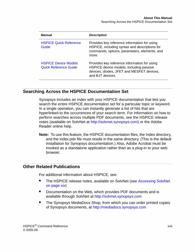
Synopsys includes an index with your HSPICE documentation that lets you search the entire HSPICE documentation set for a particular topic or keyword. In a single operation, you can instantly generate a list of hits that are hyperlinked to the occurrences of your search term. For information on how to perform searches across multiple PDF documents, see the HSPICE release notes (available on SolvNet at http://solvnet.synopsys.com) or the Adobe Reader online help.
Note: To use this feature, the HSPICE documentation files, the Index directory, and the index.pdx file must reside in the same directory. (This is the default installation for Synopsys documentation.) Also, Adobe Acrobat must be invoked as a standalone application rather than as a plug-in to your web browser.
Other Related Publications
For additional information about HSPICE, see:■ The HSPICE release notes, available on SolvNet (see Accessing SolvNet
on page xix) ■ Documentation on the Web, which provides PDF documents and is
available through SolvNet at http://solvnet.synopsys.com■ The Synopsys MediaDocs Shop, from which you can order printed copies
of Synopsys documents, at http://mediadocs.synopsys.com
HSPICE Quick Reference Guide
Provides key reference information for using HSPICE, including syntax and descriptions for commands, options, parameters, elements, and more.
HSPICE Device Models Quick Reference Guide
Provides key reference information for using HSPICE device models, including passive devices, diodes, JFET and MESFET devices, and BJT devices.
Manual Description
HSPICE® Command Reference xviiX-2005.09

About This ManualConventions
You might also want to refer to the documentation for the following related Synopsys products:■ CosmosScope■ Aurora■ Raphael■ VCS
Conventions
The following conventions are used in Synopsys documentation:
Convention Description
Courier Indicates command syntax.
Italic Indicates a user-defined value, such as object_name.
Bold Indicates user input—text you type verbatim—in syntax and examples.
[ ] Denotes optional parameters, such as
write_file [-f filename]
... Indicates that a parameter can be repeated as many times as necessary:
pin1 [pin2 ... pinN]
| Indicates a choice among alternatives, such as
low | medium | high
\ Indicates a continuation of a command line.
/ Indicates levels of directory structure.
Edit > Copy Indicates a path to a menu command, such as opening the Edit menu and choosing Copy.
Control-c Indicates a keyboard combination, such as holding down the Control key and pressing c.
xviii HSPICE® Command ReferenceX-2005.09

About This ManualCustomer Support
Customer Support
Customer support is available through SolvNet online customer support and through contacting the Synopsys Technical Support Center.
Accessing SolvNet
SolvNet includes an electronic knowledge base of technical articles and answers to frequently asked questions about Synopsys tools. SolvNet also gives you access to a wide range of Synopsys online services, which include downloading software, viewing Documentation on the Web, and entering a call to the Support Center.
To access SolvNet:
1. Go to the SolvNet Web page at http://solvnet.synopsys.com.
2. If prompted, enter your user name and password. (If you do not have a Synopsys user name and password, follow the instructions to register with SolvNet.)
If you need help using SolvNet, click SolvNet Help in the Support Resources section.
Contacting the Synopsys Technical Support Center
If you have problems, questions, or suggestions, you can contact the Synopsys Technical Support Center in the following ways:■ Open a call to your local support center from the Web by going to
http://solvnet.synopsys.com (Synopsys user name and password required), then clicking “Enter a Call to the Support Center.”
■ Send an e-mail message to your local support center.
• E-mail [email protected] from within North America.
• Find other local support center e-mail addresses at http://www.synopsys.com/support/support_ctr.
■ Telephone your local support center.
• Call (800) 245-8005 from within the continental United States.
HSPICE® Command Reference xixX-2005.09

About This ManualCustomer Support
• Call (650) 584-4200 from Canada.■ Find other local support center telephone numbers at
http://www.synopsys.com/support/support_ctr.
xx HSPICE® Command ReferenceX-2005.09

11Command Categories
Lists all commands you can use in HSPICE, arranged by task.
Alter Blocks
Use these commands in your HSPICE netlist to run alternative simulations of your netlist by using different data.
Analysis
Use these commands in your HSPICE netlist to start different types of HSPICE analysis to save the simulation results into a file, and to load the results of a previous simulation into a new simulation.
.ALIAS .ALTER .DEL LIB
.TEMP
.AC .LIN .SAMPLE
.DC .NET .SENS
.DCMATCH .NOISE .TEMP
HSPICE® Command Reference 1X-2005.09

1: Command CategoriesConditional Block
Conditional Block
Use these commands in your HSPICE netlist to setup a conditional block. HSPICE does not execute the commands in the conditional block, unless the specified conditions are true.
Digital Vector
Use these commands in your digital vector (VEC) file.
Encryption
Use these commands in your HSPICE netlist to mark the start and end of an encrypted section of a netlist.
.DISTO .OP .TF
.FFT .PAT .TRAN
.FOUR .PZ
.ELSE .ELSEIF .ENDIF
.IF
ENABLE SLOPE VIH
IDELAY TDELAY VIL
IO TFALL VNAME
ODELAY TRISE VOH
OUT or OUTZ TRIZ VOL
PERIOD TSKIP VREF
RADIX TUNIT VTH
.PROTECT .UNPROTECT
2 HSPICE® Command ReferenceX-2005.09

1: Command CategoriesField Solver
Field Solver
Use these commands in your HSPICE netlist to define a field solver.
Files
Use this command in your HSPICE netlist to call other files that are not part of the netlist.
Input/Output Buffer Information Specification (IBIS)
Use these commands in your HSPICE netlist for specifying input/output buffer information.
Library Management
Use these commands in your HSPICE netlist to manage libraries of circuit designs, and to call other files when simulating your netlist.
.FSOPTIONS .LAYERSTACK .MATERIAL
.SHAPE
.VEC
.EBD .IBIS .ICM
.PKG
.DEL LIB .INCLUDE .PROTECT
.ENDL .LIB .UNPROTECT
3 HSPICE® Command ReferenceX-2005.09
1: Command CategoriesModel Definition
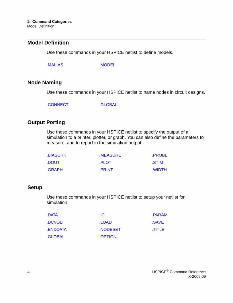
Model Definition
Use these commands in your HSPICE netlist to define models.
Node Naming
Use these commands in your HSPICE netlist to name nodes in circuit designs.
Output Porting
Use these commands in your HSPICE netlist to specify the output of a simulation to a printer, plotter, or graph. You can also define the parameters to measure, and to report in the simulation output.
Setup
Use these commands in your HSPICE netlist to setup your netlist for simulation.
.MALIAS .MODEL
.CONNECT .GLOBAL
.BIASCHK .MEASURE .PROBE
.DOUT .PLOT .STIM
.GRAPH .PRINT .WIDTH
.DATA .IC .PARAM
.DCVOLT .LOAD .SAVE
.ENDDATA .NODESET .TITLE
.GLOBAL .OPTION
4 HSPICE® Command ReferenceX-2005.09

1: Command CategoriesSimulation Runs
Simulation Runs
Use these commands in your HSPICE netlist to mark the start and end of individual simulation runs, and conditions that apply throughout an individual simulation run.
Subcircuits
Use these commands in your HSPICE netlist to define subcircuits, and to add instances of subcircuits to your netlist.
Verilog-A
Use the following command in your HSPICE netlist to declare the Verilog-A source name and path within the netlist.
.END .TEMP .TITLE
.ENDS .INCLUDE .MODEL
.EOM .MACRO .SUBCKT
.HDL
5 HSPICE® Command ReferenceX-2005.09

1: Command CategoriesVerilog-A
6 HSPICE® Command ReferenceX-2005.09

22Commands in HSPICE Netlists
Contains an alphabetical listing of all commands you can use in an HSPICE netlist.
Here are the commands described in this chapter. For a list of commands grouped according to tasks that use each command, see Chapter 1, Command Categories.
.AC .FSOPTIONS .OPTION
.ALIAS .GLOBAL .PARAM
.ALTER .GRAPH .PAT
.BIASCHK .HDL .PKG
.CONNECT .IBIS .PLOT
.DATA .IC .PRINT
.DC .ICM .PROBE
.DCMATCH .IF .PROTECT
.DCVOLT .INCLUDE .PZ
HSPICE® Command Reference 7X-2005.09

2: Commands in HSPICE Netlists
.DEL LIB .LAYERSTACK .SAMPLE
.DISTO .LIB .SAVE
.DOUT .LIN .SENS
.EBD .LOAD .SHAPE
.ELSE .MACRO .STIM
.ELSEIF .MALIAS .SUBCKT
.END .MATERIAL .TEMP
.ENDDATA .MEASURE .TF
.ENDIF .MODEL .TITLE
.ENDL .NET .TRAN
.ENDS .NODESET .UNPROTECT
.EOM .NOISE .VEC
.FFT .OP .WIDTH
.FOUR
8 HSPICE® Command ReferenceX-2005.09

2: Commands in HSPICE Netlists.AC
.AC
Syntax
Single/Double Sweep
.AC type np fstart fstop
.AC type np fstart fstop <SWEEP var <START=>start + <STOP=>stop <STEP=>incr>
.AC type np fstart fstop <SWEEP var type np start stop>
.AC type np fstart fstop + <SWEEP var START="param_expr1" + STOP="param_expr2" STEP="param_expr3">
.AC type np fstart fstop <SWEEP var start_expr + stop_expr step_expr>
Sweep Using Parameters
.AC type np fstart fstop <SWEEP DATA = datanm>
.AC DATA = datanm
.AC DATA = datanm <SWEEP var <START=>start <STOP=>stop+ <STEP=>incr>
.AC DATA = datanm <SWEEP var type np start stop>
.AC DATA = datanm <SWEEP var START="param_expr1" + STOP="param_expr2" STEP="param_expr3">
.AC DATA = datanm <SWEEP var start_expr stop_expr + step_expr>
In HSPICE RF, you can run a parameter sweep around a single analysis, but the parameter sweep cannot change .OPTION values.
Optimization
.AC DATA = datanm OPTIMIZE = opt_par_fun+ RESULTS = measnames MODEL = optmod
HSPICE RF supports optimization for bisection only.
HSPICE® Command Reference 9X-2005.09
2: Commands in HSPICE Netlists.AC
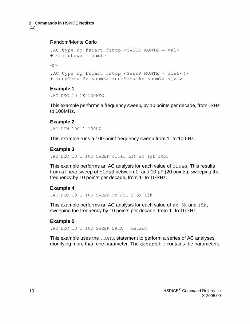
Random/Monte Carlo
.AC type np fstart fstop <SWEEP MONTE = val>+ <firstrun = num1>
-or-
.AC type np fstart fstop <SWEEP MONTE = list<(>+ <num1:num2> <num3> <num5:num6> <num7> <)> >
Example 1.AC DEC 10 1K 100MEG
This example performs a frequency sweep, by 10 points per decade, from 1kHz to 100MHz.
Example 2.AC LIN 100 1 100HZ
This example runs a 100-point frequency sweep from 1- to 100-Hz.
Example 3.AC DEC 10 1 10K SWEEP cload LIN 20 1pf 10pf
This example performs an AC analysis for each value of cload. This results from a linear sweep of cload between 1- and 10-pF (20 points), sweeping the frequency by 10 points per decade, from 1- to 10-kHz.
Example 4.AC DEC 10 1 10K SWEEP rx POI 2 5k 15k
This example performs an AC analysis for each value of rx, 5k and 15k, sweeping the frequency by 10 points per decade, from 1- to 10-kHz.
Example 5.AC DEC 10 1 10K SWEEP DATA = datanm
This example uses the .DATA statement to perform a series of AC analyses, modifying more than one parameter. The datanm file contains the parameters.
10 HSPICE® Command ReferenceX-2005.09

2: Commands in HSPICE Netlists.AC
Example 6.AC DEC 10 1 10K SWEEP MONTE = 30
This example illustrates a frequency sweep, and a Monte Carlo analysis (not supported in HSPICE RF) with 30 trials.
Example 7AC DEC 10 1 10K SWEEP MONTE = 10 firstrun=15
This example illustrates a frequency sweep and a Monte Carlo analysis from the 15th to the 24th trials.
Example 8.AC DEC 10 1 10K SWEEP MONTE = list(10 20:30 35:40 50)
This example illustrates a frequency sweep and a Monte Carlo analysis at 10th trial, and then from the 20th to 30th trial, followed by the 35th to 40th trial, and finally at 50th trial.
DescriptionYou can use the.AC statement in several different formats, depending on the application as shown in the examples. You can also use the .AC statement to perform data-driven analysis in HSPICE.
If the input file includes an .AC statement, HSPICE runs AC analysis for the circuit, over a selected frequency range for each parameter in the second sweep.
For AC analysis, the data file must include at least one independent AC source element statement (for example, VI INPUT GND AC 1V). HSPICE checks for this condition, and reports a fatal error if you did not specify such AC sources.
You also cannot use this statement in HSPICE RF.
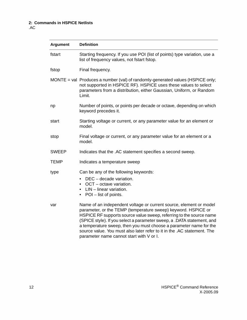
Argument Definition
DATA =datanm
Data name, referenced in the .AC statement (not supported in HSPICE RF).
incr Increment value of the voltage, current, element, or model parameter. If you use type variation, specify the np (number of points) instead of incr.
HSPICE® Command Reference 11X-2005.09
2: Commands in HSPICE Netlists.AC
fstart Starting frequency. If you use POI (list of points) type variation, use a list of frequency values, not fstart fstop.
fstop Final frequency.
MONTE = val Produces a number (val) of randomly-generated values (HSPICE only; not supported in HSPICE RF). HSPICE uses these values to select parameters from a distribution, either Gaussian, Uniform, or Random Limit.
np Number of points, or points per decade or octave, depending on which keyword precedes it.
start Starting voltage or current, or any parameter value for an element or model.
stop Final voltage or current, or any parameter value for an element or a model.
SWEEP Indicates that the .AC statement specifies a second sweep.
TEMP Indicates a temperature sweep
type Can be any of the following keywords:
• DEC – decade variation.• OCT – octave variation. • LIN – linear variation.• POI – list of points.
var Name of an independent voltage or current source, element or model parameter, or the TEMP (temperature sweep) keyword. HSPICE or HSPICE RF supports source value sweep, referring to the source name (SPICE style). If you select a parameter sweep, a .DATA statement, and a temperature sweep, then you must choose a parameter name for the source value. You must also later refer to it in the .AC statement. The parameter name cannot start with V or I.
Argument Definition
12 HSPICE® Command ReferenceX-2005.09

2: Commands in HSPICE Netlists.AC
See Also.DC.TRAN
firstrun The val value specifies the number of Monte Carlo iterations to perform. The firstrun value specifies the desired number of iterations. HSPICE runs from num1 to num1+val-1.
list The iterations at which HSPICE performs a Monte Carlo analysis. You can write more than one number after list. The colon represents "from ... to ...". Specifying only one number makes HSPICE run at only the specified point.
Argument Definition
HSPICE® Command Reference 13X-2005.09

2: Commands in HSPICE Netlists.ALIAS
.ALIAS
Syntax.ALIAS <model_name1> <model_name2>
Example 1You delete a library named poweramp, that contains a model named pa1. Another library contains an equivalent model named par1. You can then alias the pa1 model name to the par1 model name:
.ALIAS pa1 par1
During simulation when HSPICE encounters a model named pa1 in your netlist, it initially cannot find this model because you used a .ALTER statement to delete the library that contained the model. However, the .ALIAS statement indicates to use the par1 model in place of the old pa1 model and HSPICE does find this new model in another library, so simulation continues.
You must specify an old model name and a new model name to use in its place. You cannot use .ALIAS without any model names:
.ALIAS
or with only one model name:
.ALIAS pa1
You also cannot alias a model name to more than one model name, because then the simulator would not know which of these new models to use in place of the deleted or renamed model:
.ALIAS pa1 par1 par2
For the same reason, you cannot alias a model name to a second model name, and then alias the second model name to a third model name:
.ALIAS pa1 par1
.ALIAS par1 par2
If your netlist does not contain an .ALTER command, and if the .ALIAS does not report a usage error, then the .ALIAS does not affect the simulation results.
14 HSPICE® Command ReferenceX-2005.09

2: Commands in HSPICE Netlists.ALIAS
Example 2Your netlist might contain the statement:
.ALIAS myfet nfet
Without a .ALTER statement, HSPICE does not use nfet to replace myfet during simulation.
If your netlist contains one or more .ALTER commands, the first simulation uses the original myfet model. After the first simulation, if the netlist references myfet from a deleted library, .ALIAS substitutes nfet in place of the missing model. ■ If HSPICE finds model definitions for both myfet and nfet, it reports an
error and aborts.■ If HSPICE finds a model definition for myfet, but not for nfet, it reports a
warning, and simulation continues by using the original myfet model.■ If HSPICE finds a model definition for nfet, but not for myfet, it reports a
replacement successful message.
DescriptionYou can use .ALTER statements to rename a model to rename a library containing a model, or to delete an entire library of models in HSPICE. If your netlist references the old model name, then after you use one of these types of .ALTER statements, HSPICE no longer finds this model.
Note: HSPICE RF does not support the .ALIAS statement.
For example, if you use .DEL LIB in the .ALTER block to delete a library, the .ALTER command deletes all models in this library. If your netlist references one or more models in the deleted library, then HSPICE no longer finds the models.
To resolve this issue, HSPICE provides a .ALIAS command to let you alias the old model name to another model name that HSPICE can find in the existing model libraries.
See Also.ALTER.MALIAS
HSPICE® Command Reference 15X-2005.09

2: Commands in HSPICE Netlists.ALTER
.ALTER
Syntax.ALTER <title_string>
Example.ALTER simulation_run2
DescriptionYou can use the .ALTER statement to rerun an HSPICE simulation by using different parameters and data. HSPICE RF does not support the .ALTER statement.
Use parameter (variable) values for .PRINT and .PLOT statements, before you alter them. The .ALTER block cannot include .PRINT, .PLOT, .GRAPH or any other input/output statements. You can include analysis statements (.DC, .AC, .TRAN, .FOUR, .DISTO, .PZ, and so on) in a .ALTER block in an input netlist file.
However, if you change only the analysis type, and you do not change the circuit itself, then simulation runs faster if you specify all analysis types in one block, instead of using separate .ALTER blocks for each analysis type.
The .ALTER sequence or block can contain:■ Element statements (except source elements)■ .ALIAS statements■ .DATA statements■ .DEL LIB statements■ .IC (initial condition) and .NODESET statements■ .INCLUDE statements■ .LIB statements■ .MODEL statements■ .OP statements■ .OPTION statements■ .PARAM statements■ .TEMP statements
16 HSPICE® Command ReferenceX-2005.09

2: Commands in HSPICE Netlists.ALTER
■ .TF statements■ .TRAN, .DC, and .AC statements
Note: The .MALIAS command is not officially supported in .ALTER blocks.
See Also.OPTION MEASFILE
Argument Definition
title_string Any string up to 72 characters. HSPICE prints the appropriate title string for each .ALTER run in each section heading of the output listing, and in the graph data (.tr#) files.
HSPICE® Command Reference 17X-2005.09

2: Commands in HSPICE Netlists.BIASCHK
.BIASCHK
Syntax
As an expression monitor:
.BIASCHK 'expression' <limit = lim> <noise = ns>+ <max = max> <min = min>+ <simulation = op | dc | tr | all> <monitor = v | i | w | l >+ <tstart = time1> <tstop = time2> <autostop>
As an element and model monitor:
.BIASCHK type <region=cutoff | linear | saturation>+ terminal1=t1 <terminal2=t2> <limit=lim>+ <noise=ns> <max=max> <min=min>+ <simulation=op | dc | tr | all> <monitor=v | i | w | l>+ <name=name1, name2, ...>+ <mname=modname_1, modname_2, ...>+ <tstart=time1> <tstop=time2> <autostop>+ <except=name_1,name_2, ...>
Example 1This example uses the .BIASCHK statement to monitor an expression:
.biaschk 'v(1)' min = 'v(2)*2' simulation= op
Example 2This example uses the .BIASCHK statement to monitor an element and model type:
.biaschk nmos terminal1 = vg terminal2 = vssimulation = tr name = m1
In this example, terminal1 and terminal2 are the terminals between which you want to check.
DescriptionThe .BIASCHK statement can monitor the voltage bias, current, device-size, expression and region during analysis, and reports:■ Element name■ Time■ Terminals
18 HSPICE® Command ReferenceX-2005.09
2: Commands in HSPICE Netlists.BIASCHK
■ Bias that exceeds the limit■ Number of times the bias exceeds the limit for an element
HSPICE saves the information as both a warning and a BIASCHK summary in the *.lis file or a file you define in the .OPTION BIASFILE command option. You can use this command only for active elements, capacitors, and subcircuits.
If a model name, referenced in an active element statement, contains a period (.), then .BIASCHK reports an error. This occurs because it is unclear whether a reference such as x.123 is a model name or a sub-circuit name (123 model in the x subcircuit).
More than one simulation type or all simulation types can be set in one .BIASCHK command, and more than one region can be set in one .BIASCHK command.
Instance (element) and model names can contain wildcards, either “?” (stands for one character) or “*” (stands for 0 or more characters).
If you do not set name and mname, HSPICE checks all elements of this type for bias voltage (you must include type in the biaschk card). However, if type = subckt, at least one name or mname must be specified in the .BIASCHK command; otherwise, a warning message is issued and this command ignored.
After a simulation that uses the .BIASCHK command runs, HSPICE outputs a results summary including the element name, time, terminals, model name, and the number of times the bias exceeded the limit for a specified element.
Interactions with Other OptionsIf you set .OPTION BIAWARN to 1, HSPICE immediately outputs a warning message that includes the element name, time, terminals and model name when the limit is exceeded during the analysis you define. If you set the autostop keyword, HSPICE automatically stops at that situation.
If you set .OPTION BIASFILE, HSPICE outputs the summary into a file you define in the biasfile. Otherwise, HSPICE outputs the summary to a *.lis file.
HSPICE® Command Reference 19X-2005.09

2: Commands in HSPICE Netlists.BIASCHK
Argument Definition
type Element type to check.
MOS (C, BJT, ...)
For a monitor, type can be DIODE, BIPOLAR, BJT, JFET, MOS, NMOS, PMOS, C, or SUBCKT. When used with REGION, type can be MOS only.
terminal 1, 2
Terminals, between which HSPICE checks (that is, checks between terminal1 and terminal2):
• For MOS level 57: nd, ng, ns, ne, np, n6• For MOS level 58: nd, ngf, ns, ngb• For MOS level 59: nd, ng, ns, ne, np• For other MOS level: nd, ng, ns, nb• For capacitor: n1, n2• For diode: np, nn• For bipolar: nc, nb, ne, ns• For JFET: nd, ng, ns, nbFor type = subckt, the terminal names are those pins defined by the subcircuit definition of mname.
limit Biaschk limit that you define. Reports an error if the bias voltage (between appointed terminals of appointed elements and models) is larger than the limit.
noise Biaschk noise that you define. The default is 0.1v.
Noise-filter some of the results (the local maximum bias voltage, that is larger than the limit).
The next local max replaces the local max, if all of the following conditions are satisfied:
local_max-local_min<noise>.next local_max-local_min<noise>.
This local max is smaller than the next local max. For a parasitic diode, HSPICE ignores the smaller local max biased voltage, and does not output this voltage.
To disable this feature, set the noise detection level to 0.
max Maximum value.
20 HSPICE® Command ReferenceX-2005.09

2: Commands in HSPICE Netlists.BIASCHK
min Minimum value.
name Element name to check. If name and mname are not both set for the element type, the elements of this type are all checked. You can define more than one element name in keyword name with a comma (,) delimiter.
If doing bias checking for subcircuits:
• When both mname and name are defined while multiple name definitions are allowed, if a name is also an instance of mname, then only those names are checked, others will be ignored.
• This command is ignored if no name is an instance of mname.• For name definitions which are not of the type defined in mname will
be ignored.• If a mname is not defined, the subcircuit type is determined by the
first name definition.
mname Model name. HSPICE checks elements of the model for bias. If you define mname, then HSPICE checks all devices of this model. You can define more than one model name in keyword mname with the comma (,) delimiter.
If mname and name are not both set for the element type, the elements of this type are all checked.
If doing bias checking for subcircuits:
• Once there is one and only one mname defined, the terminal names for this .command are those pins defined by the subckt definition of mname.
• Multiple mname definitions are not allowed.• Wildcarding is not supported for mname.• If only mname is specified in subckt bias check, then all subcircuits
will be checked.
region Values can be cutoff, linear, or saturation. HSPICE monitors when the MOS device, defined in the .BIASCHK command, enters and leaves the specified region (such as cutoff).
simulation The simulation type you want to monitor. You can specify op, dc, tr (transient), and all (op, dc, and tr). The tr option is the default simulation type.
Argument Definition
HSPICE® Command Reference 21X-2005.09
2: Commands in HSPICE Netlists.BIASCHK
See Also.OPTION BIASFILE.OPTION BIAWARN
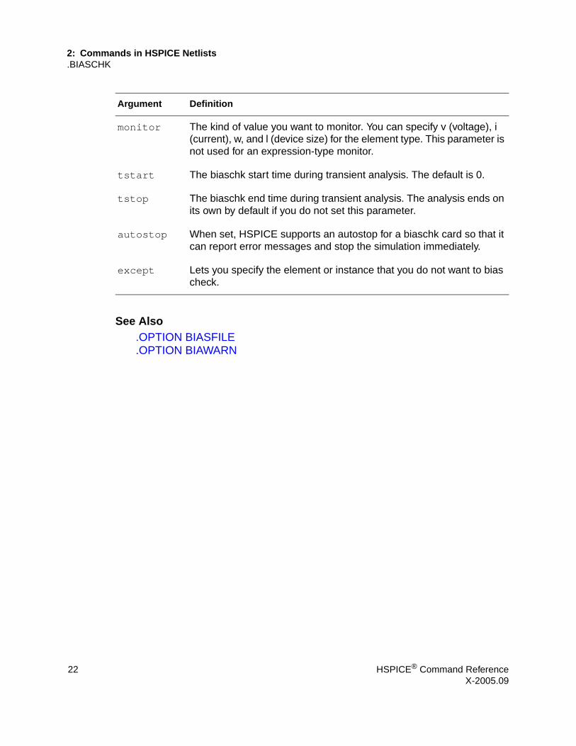
monitor The kind of value you want to monitor. You can specify v (voltage), i (current), w, and l (device size) for the element type. This parameter is not used for an expression-type monitor.
tstart The biaschk start time during transient analysis. The default is 0.
tstop The biaschk end time during transient analysis. The analysis ends on its own by default if you do not set this parameter.
autostop When set, HSPICE supports an autostop for a biaschk card so that it can report error messages and stop the simulation immediately.
except Lets you specify the element or instance that you do not want to bias check.
Argument Definition
22 HSPICE® Command ReferenceX-2005.09

2: Commands in HSPICE Netlists.CONNECT
.CONNECT
Syntax.CONNECT node1 node2
Example...
.subckt eye_diagram node1 node2 ...
.connect node1 node2
...
.ends
This is now the same as the following:
....subckt eye_diagram node1 node1 .......ends...
HSPICE reports the following error message:
**error**: subcircuit definition duplicates node node1
To apply any HSPICE statement to node2, apply it to node1 instead. Then, to change the netlist construction to recognize node2, use a .ALTER statement.
Example 2*example for .connectvcc 0 cc 5vr1 0 1 5kr2 1 cc 5k.tran 1n 10n.print i(vcc) v(1).alter.connect cc 1.end
The first .TRAN simulation includes two resistors. Later simulations have only one resistor, because r2 is shorted by connecting cc with 1. v(1) does not print out, but v(cc) prints out instead.
Use multiple .CONNECT statements to connect several nodes together.
Example 3.CONNECT node1 node2.CONNECT node2 node3
HSPICE® Command Reference 23X-2005.09

2: Commands in HSPICE Netlists.CONNECT
This example connects both node2 and node3 to node1. All connected nodes must be in the same subcircuit or all in the main circuit. The first HSPICE simulation evaluates only node1; node2, and node3 are the same node as node1. Use .ALTER statements to simulate node2 and node3.
If you set .OPTION NODE, then HSPICE prints out a node connection table.
DescriptionThe .CONNECT statement connects two nodes in your HSPICE netlist so that simulation evaluates two nodes as only one node. Both nodes must be at the same level in the circuit design that you are simulating: you cannot connect nodes that belong to different subcircuits.
If you connect node2 to node1, HSPICE does not recognize node2 at all. You also cannot use this statement in HSPICE RF.
See Also.ALTER.CONNECT.OPTION NODE
Argument Definition
node1 Name of the first of two nodes to connect to each other.
node2 Name of the second of two nodes to connect to each other. The first node replaces this node in the simulation.
24 HSPICE® Command ReferenceX-2005.09

2: Commands in HSPICE Netlists.DATA
.DATA
Syntax
Inline statement:
.DATA datanm pnam1 <pnam2 pnam3 ... pnamxxx >+ pval1<pval2 pval3 ... pvalxxx>+ pval1’ <pval2’ pval3’ ... pvalxxx’>.ENDDATA
External File statement for concatenated data files:
.DATA datanm MER+ FILE = ’filename1’ pname1 = colnum <pname2 = colnum ...>+ <FILE = ’filename2’ pname1 = colnum+ <pname2 = colnum ...>> ... <OUT = ’fileout’>.ENDDATA
Column Laminated statement:
.DATA datanm LAM+ FILE = ’filename1’ pname1 = colnum + <panme2 = colnum ...>+ <FILE = ’filename2’ pname1 = colnum + <pname2 = colnum ...>> ... <OUT = ’fileout’>.ENDDATA
Example* Inline .DATA statement
.TRAN 1n 100n SWEEP DATA = devinf
.AC DEC 10 1hz 10khz SWEEP DATA = devinf
.DC TEMP -55 125 10 SWEEP DATA = devinf
.DATA devinf width length thresh cap+ 50u 30u 1.2v 1.2pf+ 25u 15u 1.0v 0.8pf+ 5u 2u 0.7v 0.6pf
.ENDDATA
HSPICE or HSPICE RF performs the above analyses for each set of parameter values defined in the .DATA statement. For example, the program first uses the width = 50u, length = 30u, thresh = 1.2v, and cap = 1.2pf parameters to perform .TRAN, .AC, and .DC analyses.
HSPICE or HSPICE RF then repeats the analyses for width = 25u, length = 15u, thresh = 1.0v, and cap = 0.8pf, and again for the values on each subsequent line in the .DATA block.
HSPICE® Command Reference 25X-2005.09

2: Commands in HSPICE Netlists.DATA
Example 2* .DATA as the inner sweepM1 1 2 3 0 N W = 50u L = LN
VGS 2 0 0.0vVBS 3 0 VBSVDS 1 0 VDS.PARAM VDS = 0 VBS = 0 L = 1.0u.DC DATA = vdot.DATA vdot
VBS VDS L0 0.1 1.5u
0 0.1 1.0u 0 0.1 0.8u -1 0.1 1.0u
-2 0.1 1.0u -3 0.1 1.0u 0 1.0 1.0u 0 5.0 1.0u
.ENDDATA
This example performs a DC sweep analysis for each set of VBS, VDS, and L parameters in the .DATA vdot block. That is, HSPICE or HSPICE RF runs eight DC analyses, one for each line of parameter values in the .DATA block.
Example 3* .DATA as the outer sweep
.PARAM W1 = 50u W2 = 50u L = 1u CAP = 0
.TRAN 1n 100n SWEEP DATA = d1
.DATA d1W1 W2 L CAP50u 40u 1.0u 1.2pf25u 20u 0.8u 0.9pf
.ENDDATA
In this example: ■ The default start time for the .TRAN analysis is 0.■ The time increment is 1 ns.■ The stop time is 100 ns.
This results in transient analyses at every time value from 0 to 100 ns in steps of 1 ns by using the first set of parameter values in the .DATA d1 block. Then HSPICE or HSPICE RF reads the next set of parameter values, and performs another 100 transient analyses. It sweeps time from 0 to 100 ns in 1 ns steps. The outer sweep is time, and the inner sweep varies the parameter values. HSPICE or HSPICE RF performs two hundred analyses: 100 time increments, times 2 sets of parameter values.
26 HSPICE® Command ReferenceX-2005.09

2: Commands in HSPICE Netlists.DATA
Example 4* External File .DATA for concatenated data files.DATA datanm MER
+ FILE = filename1 pname1 = colnum+ <pname2 = colnum ...>+ <FILE = filename2 pname1 = colnum + <pname2 = colnum ...>>+ ...+ <OUT = fileout>
.ENDDATA
Example 5If you concatenate the three files (file1, file2, and file3).
file1 file2 file3a a a b b b c c ca a a b b b c c ca a a
The data appears as follows:
a a aa a aa a ab b bb b bc c cc c c
The number of lines (rows) of data in each file does not need to be the same. The simulator assumes that the associated parameter of each column of the A file is the same as each column of the other files.
The .DATA statement for this example is:
* External File .DATA statement.DATA inputdata MER
FILE = ‘file1’ p1 = 1 p2 = 3 p3 = 4FILE = ‘file2’ p1 = 1FILE = ‘file3’
.ENDDATA
This listing concatenates file1, file2, and file3 to form the inputdata dataset. The data in file1 is at the top of the file, followed by the data in file2, and file3. The inputdata in the .DATA statement references the dataname specified in either the .DC, .AC, or .TRAN analysis statements. The parameter fields specify the column that contains the parameters (you must already have defined the parameter names in .PARAM statements). For
HSPICE® Command Reference 27X-2005.09

2: Commands in HSPICE Netlists.DATA
example, the values for the p1 parameter are in column 1 of file1 and file2. The values for the p2 parameter are in column 3 of file1.
For data files with fewer columns than others, HSPICE or HSPICE RF assigns values of zero to the missing parameters.
Example 6Three files (D, E, and F) contain the following columns of data:
File D File E File Fd1 d2 d3 e4 e5 f6d1 d2 d3 e4 e5 f6d1 d2 d3 e4 e5 f6
The laminated data appears as follows:
d1 d2 d3 e4 e5 f6d1 d2 d3 e4 e5 f6d1 d2 d3 e4 e5 f6
The number of columns of data does not need to be the same in the three files.
The number of lines (rows) of data in each file does not need to be the same. HSPICE interprets missing data points as zero. HSPICE RF does not support column-laminated data files.
The .DATA statement for this example is:
* Column-Laminated .DATA statement.DATA dataname LAM
FILE = ‘file1’ p1 = 1 p2 = 2 p3 = 3FILE = ‘file2’ p4 = 1 p5 = 2OUT = ‘fileout’
.ENDDATA
This listing laminates columns from file1, and file2, into the fileout output file. Columns one, two, and three of file1, and columns one and two of file2, are designated as the columns to place in the output file. You can specify up to 10 files per .DATA statement.
If you run HSPICE on a different machine than the one on which the input data files reside (such as when you work over a network), use full path names instead of aliases. Aliases might have different definitions on different machines.
DescriptionData-driven analysis syntax requires a .DATA statement, and an analysis statement that contains a DATA = dataname keyword.
28 HSPICE® Command ReferenceX-2005.09
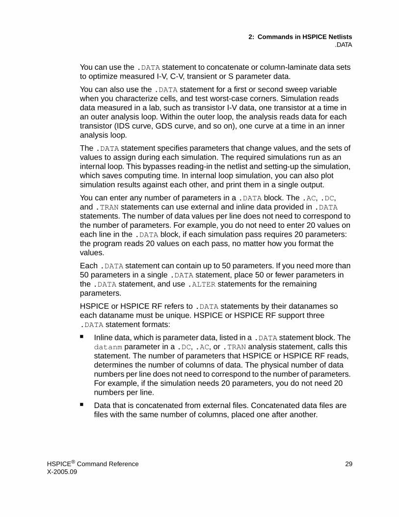
2: Commands in HSPICE Netlists.DATA
You can use the .DATA statement to concatenate or column-laminate data sets to optimize measured I-V, C-V, transient or S parameter data.
You can also use the .DATA statement for a first or second sweep variable when you characterize cells, and test worst-case corners. Simulation reads data measured in a lab, such as transistor I-V data, one transistor at a time in an outer analysis loop. Within the outer loop, the analysis reads data for each transistor (IDS curve, GDS curve, and so on), one curve at a time in an inner analysis loop.
The .DATA statement specifies parameters that change values, and the sets of values to assign during each simulation. The required simulations run as an internal loop. This bypasses reading-in the netlist and setting-up the simulation, which saves computing time. In internal loop simulation, you can also plot simulation results against each other, and print them in a single output.
You can enter any number of parameters in a .DATA block. The .AC, .DC, and .TRAN statements can use external and inline data provided in .DATA statements. The number of data values per line does not need to correspond to the number of parameters. For example, you do not need to enter 20 values on each line in the .DATA block, if each simulation pass requires 20 parameters: the program reads 20 values on each pass, no matter how you format the values.
Each .DATA statement can contain up to 50 parameters. If you need more than 50 parameters in a single .DATA statement, place 50 or fewer parameters in the .DATA statement, and use .ALTER statements for the remaining parameters.
HSPICE or HSPICE RF refers to .DATA statements by their datanames so each dataname must be unique. HSPICE or HSPICE RF support three.DATA statement formats: ■ Inline data, which is parameter data, listed in a .DATA statement block. The
datanm parameter in a .DC, .AC, or .TRAN analysis statement, calls this statement. The number of parameters that HSPICE or HSPICE RF reads, determines the number of columns of data. The physical number of data numbers per line does not need to correspond to the number of parameters. For example, if the simulation needs 20 parameters, you do not need 20 numbers per line.
■ Data that is concatenated from external files. Concatenated data files are files with the same number of columns, placed one after another.
HSPICE® Command Reference 29X-2005.09

2: Commands in HSPICE Netlists.DATA
■ Data that is column-laminated from external files. Column lamination means that the columns of files with the same number of rows, are arranged side-by-side.
To use external files with the .DATA format:■ Use the MER and LAM keywords to tell HSPICE or HSPICE RF to expect
external file data, rather than inline data. ■ Use the FILE keyword to specify the external filename. ■ You can use simple file names, such as out.dat, without the single or double
quotes ( ‘ ’ or “ ”), but use the quotes when file names start with numbers, such as “1234.dat”.
■ File names are case sensitive on Unix systems.
For data-driven analysis, specify the start time (time 0) in the analysis statement so analysis correctly calculates the stop time.
The following shows how different types of analysis use .DATA statements.
Operating point:
.DC DATA = dataname
DC sweep:
.DC vin 1 5 .25 SWEEP DATA = dataname
AC sweep:
.AC dec 10 100 10meg SWEEP DATA = dataname
TRAN sweep:
.TRAN 1n 10n SWEEP DATA = dataname
Argument Definition
colnum Column number in the data file for the parameter value. The column does not need to be the same between files.
datanm Data name, referenced in the .TRAN, .DC, or .AC statement.
filenamei Data file to read. HSPICE or HSPICE RF concatenates files in the order they appear in the .DATA statement. You can specify up to 10 files.
30 HSPICE® Command ReferenceX-2005.09

2: Commands in HSPICE Netlists.DATA
See Also.AC.DC.ENDDATA.PARAM.TRAN
fileouti Data file name, where simulation writes concatenated data. This file contains the full syntax for an inline .DATA statement, and can replace the .DATA statement that created it in the netlist. You can output the file, and use it to generate one data file from many.
LAM Column-laminated (parallel merging) data files to use.
MER Concatenated (series merging) data files to use.
pnami Parameter names, used for source value, element value, device size, model parameter value, and so on. You must declare these names in a .PARAM statement.
pvali Parameter value.
Argument Definition
HSPICE® Command Reference 31X-2005.09

2: Commands in HSPICE Netlists.DC
.DC
Syntax
Sweep or Parameterized Sweep:
.DC var1 START = start1 STOP = stop1 STEP = incr1
.DC var1 START = <param_expr1> + STOP = <param_expr2> STEP = <param_expr3>
.DC var1 start1 stop1 incr1 + <SWEEP var2 type np start2 stop2>
.DC var1 start1 stop1 incr1 <var2 start2 stop2 incr2>
HSPICE supports the start and stop syntax; HSPICE RF does not.
Data-Driven Sweep:
.DC var1 type np start1 stop1 <SWEEP DATA = datanm>
.DC DATA = datanm<SWEEP var2 start2 stop2 incr2>
.DC DATA = datanm
HSPICE supports the start and stop syntax; HSPICE RF does not.
Monte Carlo:
.DC var1 type np start1 stop1 <SWEEP MONTE = val>
.DC MONTE = val
HSPICE supports Monte Carlo analysis; HSPICE RF does not.
Optimization:
.DC DATA = datanm OPTIMIZE = opt_par_fun+ RESULTS = measnames MODEL = optmod
.DC var1 start1 stop1 SWEEP OPTIMIZE = OPTxxx + RESULTS = measname MODEL = optmod
32 HSPICE® Command ReferenceX-2005.09
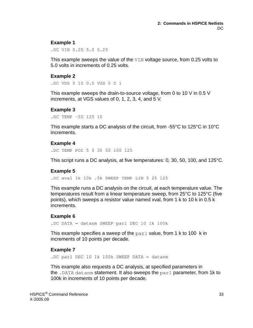
2: Commands in HSPICE Netlists.DC
Example 1.DC VIN 0.25 5.0 0.25
This example sweeps the value of the VIN voltage source, from 0.25 volts to 5.0 volts in increments of 0.25 volts.
Example 2.DC VDS 0 10 0.5 VGS 0 5 1
This example sweeps the drain-to-source voltage, from 0 to 10 V in 0.5 V increments, at VGS values of 0, 1, 2, 3, 4, and 5 V.
Example 3.DC TEMP -55 125 10
This example starts a DC analysis of the circuit, from -55°C to 125°C in 10°C increments.
Example 4.DC TEMP POI 5 0 30 50 100 125
This script runs a DC analysis, at five temperatures: 0, 30, 50, 100, and 125°C.
Example 5.DC xval 1k 10k .5k SWEEP TEMP LIN 5 25 125
This example runs a DC analysis on the circuit, at each temperature value. The temperatures result from a linear temperature sweep, from 25°C to 125°C (five points), which sweeps a resistor value named xval, from 1 k to 10 k in 0.5 k increments.
Example 6.DC DATA = datanm SWEEP par1 DEC 10 1k 100k
This example specifies a sweep of the par1 value, from 1 k to 100 k in increments of 10 points per decade.
Example 7.DC par1 DEC 10 1k 100k SWEEP DATA = datanm
This example also requests a DC analysis, at specified parameters in the .DATA datanm statement. It also sweeps the par1 parameter, from 1k to 100k in increments of 10 points per decade.
HSPICE® Command Reference 33X-2005.09

2: Commands in HSPICE Netlists.DC
Example 8.DC par1 DEC 10 1k 100k SWEEP MONTE = 30
This example invokes a DC sweep of the par1 parameter from 1k to 100k by 10 points per decade by using 30 randomly generated (Monte Carlo) values HSPICE supports Monte Carlo analysis; HSPICE RF does not.
Example 9* Schmitt Trigger Example *file: bjtschmt.sp bipolar schmitt trigger.OPTION post = 2vcc 6 0 dc 12vin 1 0 dc 0 pwl(0,0 2.5u,12 5u,0)cb1 2 4 .1pfrc1 6 2 1krc2 6 5 1krb1 2 4 5.6krb2 4 0 4.7kre 3 0 .47kdiode 0 1 dmodq1 2 1 3 bmod 1 ic = 0,8q2 5 4 3 bmod 1 ic = .5,0.2.dc vin 0,12,.1.model dmod d is = 1e-15 rs = 10.model bmod npn is = 1e-15 bf = 80 tf = 1n+ cjc = 2pf cje = 1pf rc = 50 rb = 100 vaf = 200.plot v(1) v(5).graph dc model = schmittplot input = v(1) + output = v(5) 4.0 5.0.model schmittplot plot xscal = 1 yscal = 1 + xmin = .5u xmax = 1.2u.end
Example 10.DC par1 DEC 10 1k 100k SWEEP MONTE = 10 firstrun = 11
This example invokes a DC sweep of the par1 parameter from 1k to 100k by 10 points per decade and uses 10 randomly generated (Monte Carlo) values from 11th to 20th trials.
Example 11.DC par1 DEC 10 1k 100k SWEEP MONTE = list(10 20:30 35:40 50)
This example invokes a DC sweep of the par1 parameter from 1k to 100k by 10 points per decade and a Monte Carlo analysis at the 10th trial, then from the 20th to the 30th, followed by the 35th to 40th trials, and finally at the 50th trial.
34 HSPICE® Command ReferenceX-2005.09

2: Commands in HSPICE Netlists.DC
DescriptionYou can use the .DC statement in DC analysis, to: ■ Sweep any parameter value (HSPICE and HSPICE RF).■ Sweep any source value (HSPICE and HSPICE RF).■ Sweep temperature range (HSPICE and HSPICE RF).■ Perform a DC Monte Carlo (random sweep) analysis (HSPICE only; not
supported in HSPICE RF).■ Perform a data-driven sweep (HSPICE and HSPICE RF).■ Perform a DC circuit optimization for a data-driven sweep (HSPICE and
HSPICE RF).■ Perform a DC circuit optimization by using start and stop (HSPICE only; not
supported in HSPICE RF).■ Perform a DC model characterization (HSPICE only; not supported in
HSPICE RF).
The format for the .DC statement depends on the application that uses it.
Argument Definition
DATA = datanm Datanm is the reference name of a .DATA statement.
incr1 … Voltage, current, element, or model parameters; or temperature increments.
MODEL Specifies the optimization reference name. The .MODEL OPT statement uses this name in an optimization analysis
MONTE = val val is the number of randomly-generated values, which you can use to select parameters from a distribution. The distribution can be Gaussian, Uniform, or Random Limit.
np Number of points per decade or per octave or just number of points, based on which keyword precedes it.
OPTIMIZE Specifies the parameter reference name, used for optimization in the .PARAM statement
RESULTS Measure name used for optimization in the .MEASURE statement
HSPICE® Command Reference 35X-2005.09

2: Commands in HSPICE Netlists.DC
start1 … Starting voltage, current, element, or model parameters; or temperature values. If you use the POI (list of points) variation type, specify a list of parameter values, instead of start stop.
HSPICE supports the start and stop syntax; HSPICE RF does not.
stop1 … Final voltage, current, any element, model parameter, or temperature values.
SWEEP Indicates that a second sweep has a different type of variation (DEC, OCT, LIN, POI, or DATA statement; or MONTE = val)
TEMP Indicates a temperature sweep.
type Can be any of the following keywords:
• DEC — decade variation • OCT — octave variation • LIN — linear variation • POI — list of points
var1 … • Name of an independent voltage or current source, or• Name of any element or model parameter, or • TEMP keyword (indicating a temperature sweep). HSPICE supports a source value sweep, which refers to the source name (SPICE style). However, if you select a parameter sweep, a .DATA statement, and a temperature sweep, then you must select a parameter name for the source value. A later .DC statement must refer to this name. The parameter name must not start with V, I, or TEMP.
In HSPICE RF, you can run a parameter sweep around a single analysis, but the parameter sweep cannot change any .OPTION value.
firstrun The val value specifies the number of Monte Carlo iterations to perform. The firstrun value specifies the desired number of iterations. HSPICE runs from num1 to num1+val-1.
list The iterations at which HSPICE performs a Monte Carlo analysis. You can write more than one number after list. The colon represents "from ... to ...". Specifying only one number makes HSPICE run at only the specified point.
Argument Definition
36 HSPICE® Command ReferenceX-2005.09

2: Commands in HSPICE Netlists.DC
See Also.MODEL.OPTION DCIC.PARAM
HSPICE® Command Reference 37X-2005.09

2: Commands in HSPICE Netlists.DCMATCH
.DCMATCH
Syntax.DCMATCH OUTVAR <THRESHOLD=T> <FILE=string>+ <PERTURBATION=P> <INTERVAL=Int>
Example 1.DCmatch V(9) V(4,2) I(VCC)
HSPICE reports DCmatch variations on the voltage of node 9, the voltage difference between nodes 4 and 2, and on the current through the source VCC.
Example 2.DC XVal Start=1K Stop=9K Step=1K.DCMATCH V(vcc) interval=3
The variable XVal is being sweep in the .DC command. It takes nine values in sequence from 1k to 9k in increments of 1k. Tabular output for the .DCMATCH command is only generated for the set XVal={1k, 4k, 7k, 9k}.
DescriptionYou use this command to calculate the effects of local variations in device characteristics on the DC solution of a circuit.
You can perform only one DCMATCH analysis per simulation. Only the last .DCMATCH statement is used in case more than one in present. The others are discarded with warnings.
.
Argument Definition
OUTVAR Valid node voltages, the difference between node pairs or branch currents.
THRESHOLD Report devices with a relative contribution above Threshold in the summary table.
• T=0: reports results for all devices• T<0: suppresses table output; however, individual results are
still available through .PROBE or .MEASURE statements. The upper limit for T is 1, but at least 10 devices are reported, or all if there are less than 10. Default value is 0.01.
38 HSPICE® Command ReferenceX-2005.09

2: Commands in HSPICE Netlists.DCMATCH
See Also.DC.MEASURE (Average, RMS, MIN, MAX, INTEG, and PP).MEASURE (Equation Evaluation/ Arithmetic Expression).MEASURE (FIND and WHEN).PROBE
FILE Valid file name for the output tables. Default is basename.dm# where “#” is the usual sequence number for HSPICE output files.
PERTURBATION Indicates that perturbations of P standard deviation will be used in calculating the finite difference approximations to device derivatives. The valid range for P is 0.01 to 6, with a default value of 2.
INTERVAL Applies only if a DC sweep is specified. Int is a positive integer. A summary is printed at the first sweep point, then for each subsequent increment of Int, and then, if not already printed, at the final sweep point. Only single sweeps are supported.
Argument Definition
HSPICE® Command Reference 39X-2005.09

2: Commands in HSPICE Netlists.DCVOLT
.DCVOLT
Syntax.DCVOLT V(node1) = val1 V(node2) = val2 ...
.DCVOLT V node1 val1 <node2 val2 ...>
Example.DCVOLT 11 5 4 -5 2 2.2
DescriptionUse the .IC statement or the .DCVOLT statement to set transient initial conditions in HSPICE, but not in HSPICE RF. How it initializes depends on whether the .TRAN analysis statement includes the UIC parameter.
Note: In HSPICE RF, .IC is always set to OFF.
If you specify the UIC parameter in the .TRAN statement, HSPICE does not calculate the initial DC operating point, but directly enters transient analysis. Transient analysis uses the .IC initialization values as part of the solution for timepoint zero (calculating the zero timepoint applies a fixed equivalent voltage source). The .IC statement is equivalent to specifying the IC parameter on each element statement, but is more convenient. You can still specify the IC parameter, but it does not have precedence over values set in the .IC statement.
If you do not specify the UIC parameter in the .TRAN statement, HSPICE computes the DC operating point solution, before the transient analysis. The node voltages that you specify in the .IC statement are fixed to determine the DC operating point. HSPICE RF does not output node voltage from operating point (.OP), if time (t) < 0. Transient analysis releases the initialized nodes to calculate the second and later time points.
Argument Definition
val1 ... Specifies voltages. The significance of these voltages depends on whether you specify the UIC parameter in the .TRAN statement.
node1 ... Node numbers or names can include full paths or circuit numbers.
40 HSPICE® Command ReferenceX-2005.09

2: Commands in HSPICE Netlists.DCVOLT
See Also.IC.TRAN
HSPICE® Command Reference 41X-2005.09

2: Commands in HSPICE Netlists.DEL LIB
.DEL LIB
Syntax.DEL LIB ‘<filepath>filename’ entryname
.DEL LIB libnumber entryname
Example 1This example uses an .ALTER block so it applies to HSPICE but not to HSPICE RF.
FILE1: ALTER1 TEST CMOS INVERTER.OPTION ACCT LIST.TEMP 125.PARAM WVAL = 15U VDD = 5*.OP.DC VIN 0 5 0.1.PLOT DC V(3) V(2)*VDD 1 0 VDDVIN 2 0*M1 3 2 1 1 P 6U 15UM2 3 2 0 0 N 6U W = WVAL*
.LIB 'MOS.LIB' NORMAL
.ALTER.DEL LIB 'MOS.LIB' NORMAL $removes LIB from memory
$PROTECTION.PROT $protect statements
$below .PROT.LIB 'MOS.LIB' FAST $get fast model library
.UNPROT.ALTER.OPTION NOMOD OPTS $suppress printing model
$parameters and print the $option summary
.TEMP -50 0 50 $run with different $temperatures
.PARAM WVAL = 100U VDD = 5.5 $change the parametersVDD 1 0 5.5 $using VDD 1 0 5.5 to
$change the power supply $VDD value doesn't $work
VIN 2 0 PWL 0NS 0 2NS 5 4NS 0 5NS 5$change the input
$source
42 HSPICE® Command ReferenceX-2005.09
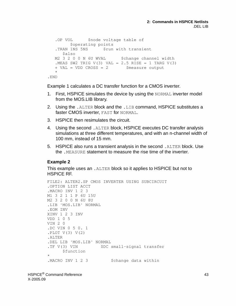
2: Commands in HSPICE Netlists.DEL LIB
.OP VOL $node voltage table of $operating points
.TRAN 1NS 5NS $run with transient $also
M2 3 2 0 0 N 6U WVAL $change channel width.MEAS SW2 TRIG V(3) VAL = 2.5 RISE = 1 TARG V(3)+ VAL = VDD CROSS = 2 $measure output*
.END
Example 1 calculates a DC transfer function for a CMOS inverter.
1. First, HSPICE simulates the device by using the NORMAL inverter model from the MOS.LIB library.
2. Using the .ALTER block and the .LIB command, HSPICE substitutes a faster CMOS inverter, FAST for NORMAL.
3. HSPICE then resimulates the circuit.
4. Using the second .ALTER block, HSPICE executes DC transfer analysis simulations at three different temperatures, and with an n-channel width of 100 mm, instead of 15 mm.
5. HSPICE also runs a transient analysis in the second .ALTER block. Use the .MEASURE statement to measure the rise time of the inverter.
Example 2This example uses an .ALTER block so it applies to HSPICE but not to HSPICE RF.
FILE2: ALTER2.SP CMOS INVERTER USING SUBCIRCUIT.OPTION LIST ACCT.MACRO INV 1 2 3 M1 3 2 1 1 P 6U 15UM2 3 2 0 0 N 6U 8U.LIB 'MOS.LIB' NORMAL.EOM INVXINV 1 2 3 INV VDD 1 0 5VIN 2 0 .DC VIN 0 5 0. 1.PLOT V(3) V(2).ALTER.DEL LIB 'MOS.LIB' NORMAL.TF V(3) VIN $DC small-signal transfer
$function*.MACRO INV 1 2 3 $change data within
HSPICE® Command Reference 43X-2005.09

2: Commands in HSPICE Netlists.DEL LIB
$subcircuit defM1 4 2 1 1 P 100U 100U $change channel
$length,width,also$topology
M2 4 2 0 0 N 6U 8U $change topologyR4 4 3 100 $add the new elementC3 3 0 10P $add the new element.LIB 'MOS.LIB' SLOW $set slow model library$.INC 'MOS2.DAT' $not allowed to be used
$inside subcircuit, allowed $outside subcircuit
.EOM INV
.END
In this example, the .ALTER block adds a resistor and capacitor network to the circuit. The network connects to the output of the inverter, and HSPICE simulates a DC small-signal transfer function.
DescriptionUse the .DEL LIB statement to remove library data from memory. The next time you run a simulation, the .DEL LIB statement removes the .LIB call statement with the same library number and entry name, from memory. You can then use a .LIB statement to replace the deleted library.
You can use the .DEL LIB statement with the .ALTER statement. HSPICE RF does not support the .ALTER statement.
Argument Definition
entryname Entry name, used in the library call statement to delete.
filename Name of a file to delete from the data file. The file path, plus the file name, can be up to 256 characters long. You can use any file name that is valid for the operating system that you use. Enclose the file path and file name in single or double quote marks.
filepath Path name of a file, if the operating system supports tree-structured directories.
libnumber Library number, used in the library call statement to delete.
44 HSPICE® Command ReferenceX-2005.09

2: Commands in HSPICE Netlists.DEL LIB
See Also.ALTER.LIB
HSPICE® Command Reference 45X-2005.09

2: Commands in HSPICE Netlists.DISTO
.DISTO
Syntax.DISTO Rload <inter <skw2 <refpwr <spwf>>>>
Example.DISTO RL 2 0.95 1.0E-3 0.75
DescriptionThe .DISTO statement computes the distortion characteristics of the circuit in an AC small-signal, sinusoidal, steady-state analysis. You can use the .DISTO statement in HSPICE, but not in HSPICE RF.
The program computes and reports five distortion measures at the specified load resistor. The analysis assumes that the input uses one or two signal frequencies. ■ HSPICE uses the first frequency (F1, the nominal analysis frequency) to
calculate harmonic distortion. The .AC statement frequency-sweep sets it. ■ HSPICE uses the optional second input frequency (F2) to calculate
intermodulation distortion. To set it implicitly, specify the skw2 parameter, which is the F2/F1 ratio
HSPICE performs only one distortion analysis per simulation. HSPICE RF does not support the .DISTO statement. If your design contains more than one .DISTO statement, HSPICE runs only the last statement. The .DISTO statement calculates distortions for diodes, BJTs (levels 1, 2, 3, and 4), and MOSFETs (Level49 and Level53, Version 3.22).
You can use the .DISTO command only with the .AC command.
.
Argument Definition
Rload The resistor element name of the output load resistor, into which the output power feeds.
refpwr Reference power level, used to compute the distortion products. If you omit refpwr, the default value is 1mW, measured in decibels magnitude (dbM). The value must be ≥ 1e-10.
46 HSPICE® Command ReferenceX-2005.09

2: Commands in HSPICE Netlists.DISTO
skw2 Ratio of the second frequency (F2) to the nominal analysis frequency (F1) in the range 1e-3 < skw2 < 0.999. If you omit skw2, the default value is 0.9.
spwf Amplitude of the second frequency (F2). The value must be ≥ 1e-3. Default = 1.0.
inter Interval at which HSPICE prints a distortion-measure summary. Specifies a number of frequency points in the AC sweep (see the np parameter in the .AC command).
• If you omit inter or set it to zero, HSPICE does not print a summary. To print or plot the distortion measures, use the .PRINT or .PLOT statement.
• If you set inter to 1 or higher, HSPICE prints a summary of the first frequency, and of each subsequent inter-frequency increment.
To obtain a summary printout for only the first and last frequencies, set inter equal to the total number of increments needed to reach fstop in the .AC statement. For a summary printout of only the first frequency, set inter to greater than the total number of increments required to reach fstop.
HSPICE prints an extensive summary from the distortion analysis for each frequency listed. Use the inter parameter in the .DISTO statement to limit the amount of output generated.
.DISTO Value
Description
DIM2 Intermodulation distortion, first difference. Relative magnitude and phase of the frequency component (F1 - F2).
DIM3 Intermodulation distortion, second difference. The relative magnitude and phase of the frequency component (2 ⋅ F1 - F2).
HD2 Second-order harmonic distortion. Relative magnitude and phase of the frequency component 2 ⋅ F1 (ignores F2).
Argument Definition
HSPICE® Command Reference 47X-2005.09

2: Commands in HSPICE Netlists.DISTO
See Also.AC
HD3 Third-order harmonic distortion. Relative magnitude and phase of the frequency component 3 ⋅ F1 (ignores F2).
SIM2 Intermodulation distortion, sum. Relative magnitude and phase of the frequency component (F1 + F2).
.DISTO Value
Description
48 HSPICE® Command ReferenceX-2005.09

2: Commands in HSPICE Netlists.DOUT
.DOUT
Syntax.DOUT nd VTH ( time state < time state > )
.DOUT nd VLO VHI ( time state < time state > )
The first syntax specifies a single threshold voltage, VTH. A voltage level above VTH is high; any level below VTH is low.
The second syntax defines a threshold for both a logic high (VHI) and low (VLO).
Note: If you specify VTH, VLO, and VHI in the same statement, then only VTH is processed, and VLO and VHI are ignored.
Example.PARAM VTH = 3.0.DOUT node1 VTH(0.0n 0 1.0n 1 + 2.0n X 3.0n U 4.0n Z 5.0n 0)
The .PARAM statement in this example sets the VTH variable value to 3. The .DOUT statement, operating on the node1 node, uses VTH as its threshold voltage.
When node1 is above 3V, it is a logic 1; otherwise, it is a logic 0. ■ At 0ns, the expected state of node1 is logic-low.■ At 1ns, the expected state is logic-high.■ At 2ns, 3ns, and 4ns, the expected state is “do not care”.■ At 5ns, the expected state is again logic low.
DescriptionThe digital output (.DOUT) statement specifies the expected final state of an output signal.
During simulation, HSPICE or HSPICE RF compares simulation results with the expected output. If the states are different, an error report results.
HSPICE® Command Reference 49X-2005.09

2: Commands in HSPICE Netlists.DOUT
For both syntax cases, the time, state pair describes the expected output. During simulation, the simulated results are compared against the expected output vector. If the states are different, HSPICE RF reports an error message. Legal values for state are:
Argument Definition
nd Node name.
time Absolute timepoint.
state Expected condition of the nd node at the specified time:
• 0 expect ZERO,LOW.• 1 expect ONE,HIGH.• else Don’t care.
VTH Single voltage threshold.
VLO Voltage of the logic-low state.
VHI Voltage of the logic-high state.
.DOUT State Value
Description
0 expect ZERO
1 expect ONE
X, x do not care
U, u do not care
Z, z expect HIGH IMPEDANCE (don’t care). HSPICE RF cannot detect a high impedance state so it treats Z, z as “don’t care” state.
50 HSPICE® Command ReferenceX-2005.09

2: Commands in HSPICE Netlists.DOUT
See Also.GRAPH.MEASURE.PARAM.PLOT.PRINT.PROBE.STIM
HSPICE® Command Reference 51X-2005.09

2: Commands in HSPICE Netlists.EBD
.EBD
Syntax.EBD ebdname + file = ’filename’ + model = ’modelname’ + component = ’compname:reference_designator’ + {component = ’compname:reference_designator’...}
Example.ebd ebd
+ file = ’test.ebd’+ model = ’16Meg X 8 SIMM Module’+ component = ’cmpnt:u21’
.ibis cmpnt+ file = ’ebd.ibs’+ component = ’SIMM’+ hsp_ver = 2003.09 nowarn
This example corresponds to the following .ebd file:
...................[Begin Board Description] 16Meg X 8 SIMM Module..................[Pin List] signal_nameJ25 POWER5[Path Description] CAS_2Pin J25Len = 0.5 L=8.35n C=3.34p R=0.01 /Node u21.1Len = 0.5 L=8.35n C=3.34p R=0.01 /Node u22.2Len = 0.5 L=8.35n C=3.34p R=0.01 /Node u23.3
DescriptionThe .EBD command provides the IBIS(V 3.2) EBD feature. HSPICE uses the .ebd file when simulating the line connected with the u21 reference_designator. The format of node names is ebdname_SignalName. For example, the format of a node name called J25 is ebd_POWER5 (see Figure 1).
52 HSPICE® Command ReferenceX-2005.09

2: Commands in HSPICE Netlists.EBD
Figure 1 Circuit Connection for EBD Example
See Also.IBIS.PKG
Argument Definition
compname Name of a .ibs file that describes a component.
reference_designator Reference designator that maps the component.
Pin2U22
J25Len=0.5 Len=0.5 Len=0.5
Pin1U21
Pin3U23
HSPICE® Command Reference 53X-2005.09

2: Commands in HSPICE Netlists.ELSE
.ELSE
Syntax.ELSE
Description.ELSE precedes one or more commands in a conditional block, after the last .ELSEIF statement, but before the .ENDIF statement. HSPICE executes these commands by default, if the conditions in the preceding .IF statement, and in all of the preceding .ELSEIF statements in the same conditional block, are all false.
For the syntax and a description of how to use the .ELSE statement within the context of a conditional block, see the .IF statement.
See Also.ELSEIF.ENDIF.IF
54 HSPICE® Command ReferenceX-2005.09

2: Commands in HSPICE Netlists.ELSEIF
.ELSEIF
Syntax.ELSEIF
DescriptionHSPICE executes the commands that follow the first.ELSEIF statement, only if condition1 in the preceding .IF statement is false, and condition2 in the first .ELSEIF statement is true.
If condition1 in the .IF statement and condition2 in the first .ELSEIF statement are both false, then HSPICE moves on to the next .ELSEIF statement, if there is one. If this second .ELSEIF condition is true, HSPICE executes the commands that follow the second .ELSEIF statement, instead of the commands after the first .ELSEIF statement.
HSPICE ignores the commands in all false .IF and .ELSEIF statements, until it reaches the first .ELSEIF condition that is true. If no .IF or .ELSEIF condition is true, HSPICE continues to the .ELSE statement
For the syntax and a description of how to use the .ELSEIF statement within the context of a conditional block, see the .IF statement.
See Also.ELSE.ENDIF.IF
HSPICE® Command Reference 55X-2005.09
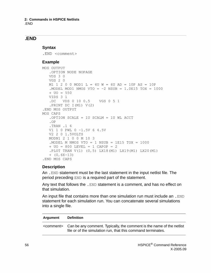
2: Commands in HSPICE Netlists.END
.END
Syntax.END <comment>
ExampleMOS OUTPUT
.OPTION NODE NOPAGEVDS 3 0VGS 2 0M1 1 2 0 0 MOD1 L = 4U W = 6U AD = 10P AS = 10P.MODEL MOD1 NMOS VTO = -2 NSUB = 1.0E15 TOX = 1000 + UO = 550VIDS 3 1.DC VDS 0 10 0.5 VGS 0 5 1.PRINT DC I(M1) V(2)
.END MOS OUTPUTMOS CAPS
.OPTION SCALE = 1U SCALM = 1U WL ACCT
.OP
.TRAN .1 6V1 1 0 PWL 0 -1.5V 6 4.5V V2 2 0 1.5VOLTSMODN1 2 1 0 0 M 10 3.MODEL M NMOS VTO = 1 NSUB = 1E15 TOX = 1000 + UO = 800 LEVEL = 1 CAPOP = 2.PLOT TRAN V(1) (0,5) LX18(M1) LX19(M1) LX20(M1) + (0,6E-13)
.END MOS CAPS
DescriptionAn .END statement must be the last statement in the input netlist file. The period preceding END is a required part of the statement.
Any text that follows the .END statement is a comment, and has no effect on that simulation.
An input file that contains more than one simulation run must include an .END statement for each simulation run. You can concatenate several simulations into a single file.
Argument Definition
<comment> Can be any comment. Typically, the comment is the name of the netlist file or of the simulation run, that this command terminates.
56 HSPICE® Command ReferenceX-2005.09

2: Commands in HSPICE Netlists.ENDDATA
.ENDDATA
Syntax.ENDDATA
DescriptionUse the .ENDDATA statement to end a .DATA block in an HSPICE input netlist.
See Also.DATA
HSPICE® Command Reference 57X-2005.09

2: Commands in HSPICE Netlists.ENDIF
.ENDIF
Syntax.ENDIF
DescriptionThe .ENDIF statement ends a conditional block of commands that begins with an .IF statement.
For the syntax and a description of how to use the .ENDIF statement within the context of a conditional block, see the .IF statement.
See Also.ELSE.ELSEIF.IF
58 HSPICE® Command ReferenceX-2005.09

2: Commands in HSPICE Netlists.ENDL
.ENDL
Syntax.ENDL
DescriptionUse the .ENDL statement to end a .LIB statement in an HSPICE input netlist.
See Also.LIB
HSPICE® Command Reference 59X-2005.09

2: Commands in HSPICE Netlists.ENDS
.ENDS
Syntax.ENDS <SUBNAME>
Example 1.ENDS mos_circuit
This example terminates a subcircuit named mos_circuit.
Example 2.ENDS
If you omit the subcircuit name as in this second example, this statement terminates all subcircuit definitions that begin with a .SUBCKT statement.
DescriptionUse the .ENDS statement to terminate a .SUBCKT statement.
This statement must be the last for any subcircuit definition that starts with a .SUBCKT command.
You can nest subcircuit references (calls) within subcircuits in HSPICE or HSPICE RF. However, in HSPICE RF, you cannot replicate output commands within subcircuit (subckt) definitions.
See Also.SUBCKT
Argument Definition
<SUBNAME> Name of the subcircuit description to terminate, that begins with a .SUBCKT command.
60 HSPICE® Command ReferenceX-2005.09
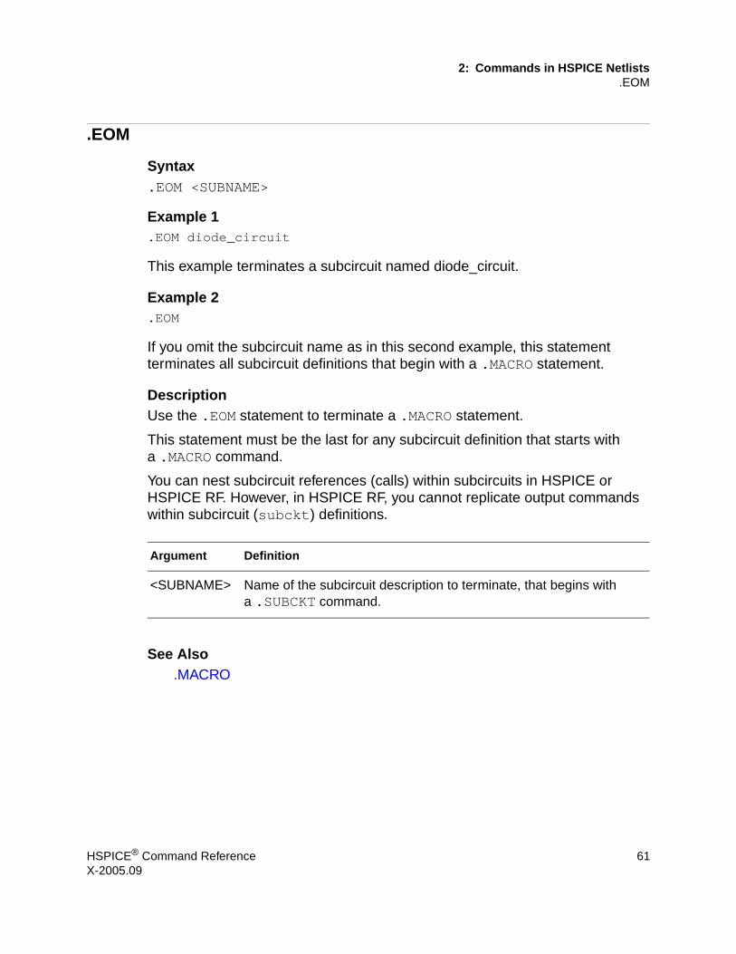
2: Commands in HSPICE Netlists.EOM
.EOM
Syntax.EOM <SUBNAME>
Example 1.EOM diode_circuit
This example terminates a subcircuit named diode_circuit.
Example 2.EOM
If you omit the subcircuit name as in this second example, this statement terminates all subcircuit definitions that begin with a .MACRO statement.
DescriptionUse the .EOM statement to terminate a .MACRO statement.
This statement must be the last for any subcircuit definition that starts with a .MACRO command.
You can nest subcircuit references (calls) within subcircuits in HSPICE or HSPICE RF. However, in HSPICE RF, you cannot replicate output commands within subcircuit (subckt) definitions.
See Also.MACRO
Argument Definition
<SUBNAME> Name of the subcircuit description to terminate, that begins with a .SUBCKT command.
HSPICE® Command Reference 61X-2005.09
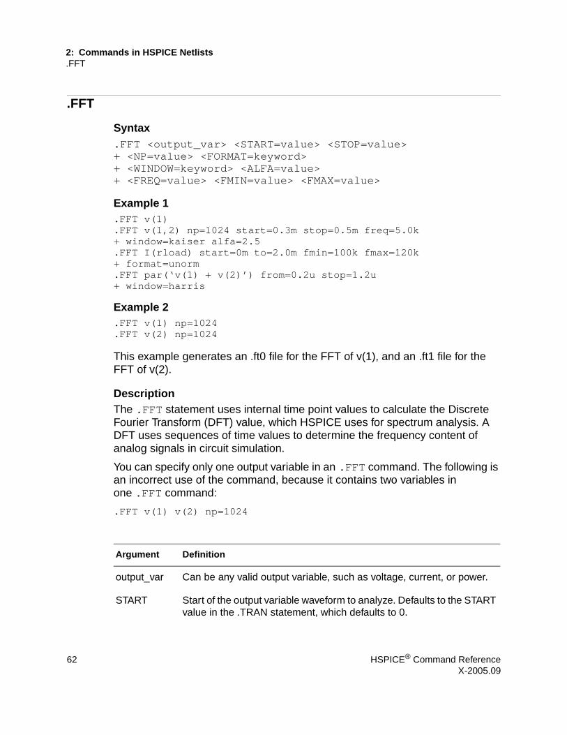
2: Commands in HSPICE Netlists.FFT
.FFT
Syntax.FFT <output_var> <START=value> <STOP=value> + <NP=value> <FORMAT=keyword> + <WINDOW=keyword> <ALFA=value>+ <FREQ=value> <FMIN=value> <FMAX=value>
Example 1.FFT v(1).FFT v(1,2) np=1024 start=0.3m stop=0.5m freq=5.0k+ window=kaiser alfa=2.5.FFT I(rload) start=0m to=2.0m fmin=100k fmax=120k+ format=unorm.FFT par(‘v(1) + v(2)’) from=0.2u stop=1.2u+ window=harris
Example 2.FFT v(1) np=1024.FFT v(2) np=1024
This example generates an .ft0 file for the FFT of v(1), and an .ft1 file for the FFT of v(2).
DescriptionThe .FFT statement uses internal time point values to calculate the Discrete Fourier Transform (DFT) value, which HSPICE uses for spectrum analysis. A DFT uses sequences of time values to determine the frequency content of analog signals in circuit simulation.
You can specify only one output variable in an .FFT command. The following is an incorrect use of the command, because it contains two variables in one .FFT command:
.FFT v(1) v(2) np=1024
Argument Definition
output_var Can be any valid output variable, such as voltage, current, or power.
START Start of the output variable waveform to analyze. Defaults to the START value in the .TRAN statement, which defaults to 0.
62 HSPICE® Command ReferenceX-2005.09

2: Commands in HSPICE Netlists.FFT
FROM An alias for START in .FFT statements.
STOP End of the output variable waveform to analyze. Defaults to the TSTOP value in the .TRAN statement.
TO An alias for STOP, in .FFT statements.
NP Number of points to use in the FFT analysis. NP must be a power of 2. If NP is not a power of 2, HSPICE automatically adjusts it to the closest higher number that is a power of 2. Default=1024.
FORMAT Specifies the output format:
• NORM= normalized magnitude (default)• UNORM=unnormalized magnitude
WINDOW Specifies the window type to use:
• RECT=simple rectangular truncation window (default).• BART=Bartlett (triangular) window.• HANN=Hanning window.• HAMM=Hamming window.• BLACK=Blackman window.• HARRIS=Blackman-Harris window.• GAUSS=Gaussian window.• KAISER=Kaiser-Bessel window.
ALFA Parameter to use in GAUSS and KAISER windows to control the highest side-lobe level, bandwidth, and so on.
1.0 <= ALFA <= 20.0
Default=3.0
FREQ Frequency to analyze. If FREQ is non-zero, the output lists only the harmonics of this frequency, based on FMIN and FMAX. HSPICE also prints the THD for these harmonics. Default=0.0 (Hz).
Argument Definition
HSPICE® Command Reference 63X-2005.09

2: Commands in HSPICE Netlists.FFT
See Also.TRAN
FMIN Minimum frequency for which HSPICE prints FFT output into the listing file. THD calculations also use this frequency.
T = (STOP-START)
Default=1.0/T (Hz).
FMAX Maximum frequency for which HSPICE prints FFT output into the listing file. THD calculations also use this frequency. Default=0.5*NP*FM IN (Hz).
Argument Definition
64 HSPICE® Command ReferenceX-2005.09
2: Commands in HSPICE Netlists.FOUR
.FOUR
Syntax.FOUR freq ov1 <ov2 ov3 ...>
Example.FOUR 100K V(5)
DescriptionThis statement performs a Fourier analysis as part of the transient analysis. You can use the .FOUR statement in or HSPICE RF to HSPICE perform the Fourier analysis over the interval (tstop-fperiod, tstop), where:■ tstop is the final time, specified for the transient analysis.■ fperiod is a fundamental frequency period (freq parameter).
HSPICE or HSPICE RF performs Fourier analysis on 501 points of transient analysis data on the last 1/f time period, where f is the fundamental Fourier frequency. HSPICE or HSPICE RF interpolates transient data to fit on 501 points, running from (tstop-1/f) to tstop.
To calculate the phase, the normalized component, and the Fourier component, HSPICE or HSPICE RF uses 10 frequency bins. The Fourier analysis determines the DC component, and the first nine AC components. For improved accuracy, the .FOUR statement can use non-linear, instead of linear interpolation.
You can only use a .FOUR statement in conjunction with a .TRAN statement.
See Also.TRAN
Argument Definition
freq Fundamental frequency
ov1 … Output variables to analyze.
HSPICE® Command Reference 65X-2005.09

2: Commands in HSPICE Netlists.FSOPTIONS
.FSOPTIONS
Syntax.FSOPTIONS name <ACCURACY=LOW|MEDIUM|HIGH> + <GRIDFACTOR=val> <PRINTDATA=YES|NO> + <COMPUTEG0=YES|NO> <COMPUTEGD=YES|NO> + <COMPUTERO=YES|NO> <COMPUTERS=YES|NO>
DescriptionUse the .FSOPTIONS statement to set various options for the field solver. The following rules apply to the Field Solver when specifying options with the .FSOPTIONS statement:■ The field solver always computes the L and C matrices.■ If COMPUTERS=YES, then the field solver starts, and calculates Lo, Ro, and
Rs.■ For each accuracy mode, the field solver uses either the pre-defined number
of segments or the number of segments that you specified. It then multiplies this number times the GRIDFACTOR to obtain the final number of segments.
Because a wide range of applications are available, the pre-defined accuracy level might not be accurate enough for some applications. If you need a higher accuracy than the value that the HIGH option sets, then increase either the GRIDFACTOR value or the N, NH, or NW values to increase the mesh density.
Argument Definition
name Option name.
ACCURACY Sets the solver accuracy to one of the following:
• LOW• MEDIUM• HIGH
GRIDFACTOR Multiplication factor (integer) to determine the final number of segments used to define the shape.
If you set COMPUTERS=yes, the field solver does not use this parameter to compute Ro and Rs values.
PRINTDATA The solver prints output matrices.
66 HSPICE® Command ReferenceX-2005.09

2: Commands in HSPICE Netlists.FSOPTIONS
See Also.LAYERSTACK.MATERIAL.SHAPE
COMPUTEGO The solver computes the static conductance matrix.
COMPUTEGD The solver computes the dielectric loss matrix.
COMPUTERO The solver computes the DC resistance matrix.
COMPUTERS The solver computes the skin-effect resistance matrix. This parameter uses the filament method solver to compute Ro and Rs.
Argument Definition
HSPICE® Command Reference 67X-2005.09

2: Commands in HSPICE Netlists.GLOBAL
.GLOBAL
Syntax.GLOBAL node1 node2 node3 ...
ExampleThis example shows global definitions for VDD and input_sig nodes.
.GLOBAL VDD input_sig
DescriptionThe .GLOBAL statement globally assigns a node name in HSPICE or HSPICE RF. This means that all references to a global node name, used at any level of the hierarchy in the circuit, connect to the same node.
The most common use of a .GLOBAL statement is if your netlist file includes subcircuits. This statement assigns a common node name to subcircuit nodes. Another common use of .GLOBAL statements is to assign power supply connections of all subcircuits. For example, .GLOBAL VCC connects all subcircuits with the internal node name VCC.
Ordinarily, in a subcircuit, the node name consists of the circuit number, concatenated to the node name. When you use a .GLOBAL statement, HSPICE or HSPICE RF does not concatenate the node name with the circuit number, and assigns only the global name. You can then exclude the power node name in the subcircuit or macro call.
Argument Definition
node1 node2 Name of a global nodes, such as supply and clock names; overrides local subcircuit definitions.
68 HSPICE® Command ReferenceX-2005.09

2: Commands in HSPICE Netlists.GRAPH
.GRAPH
Note: This is an obsolete command. You can gain the same functionality by using the .PROBE command.
Syntax.GRAPH antype <MODEL = mname> <unam1 = > ov1,+ <unam2 = >ov2 ... <unamn = >ovn (plo,phi)
Example.GRAPH DC cgb = lx18(m1) cgd = lx19(m1) + cgs = lx20(m1).GRAPH DC MODEL = plotbjt+ model_ib = i2(q1) meas_ib = par(ib)+ model_ic = i1(q1) meas_ic = par(ic)+ model_beta = par('i1(q1)/i2(q1)')+ meas_beta = par('par(ic)/par(ib)')(1e-10,1e-1).MODEL plotbjt PLOT MONO = 1 YSCAL = 2 XSCAL = 2 + XMIN = 1e-8 XMAX = 1e-1
DescriptionUse the .GRAPH statement when you need high-resolution plots of HSPICE simulation results. You cannot use .GRAPH statements in the PC version of HSPICE or in any versions of HSPICE RF.
Each .GRAPH statement creates a new .gr# file, where # ranges first from 0 to 9, and then from a to z. You can create up to 10000 graph files.
You can include wildcards in .GRAPH statements (HSPICE only).
Argument Definition
antype Type of analysis for the specified plots (outputs). Analysis types are: DC, AC, TRAN, NOISE, or DISTO (you cannot run DISTO analysis in HSPICE RF).
mname Plot model name, referenced in the .GRAPH statement. Use .GRAPH and its plot name to create high-resolution plots directly from HSPICE.
unam1… You can define output names, which correspond to the ov1 ov2 … output variables (unam1 unam2 ...), and use them as labels, instead of output variables for a high resolution graphic output.
HSPICE® Command Reference 69X-2005.09

2: Commands in HSPICE Netlists.GRAPH
See Also.DOUT.MEASURE.PLOT.PRINT.PROBE.STIM
ov1 … Output variables to print. Can be voltage, current, or element template variables (HSPICE only; HSPICE RF does not support element template output, or .GRAPH statements), from a different type of analysis. You can also use algebraic expressions as output variables, but you must define them inside the PAR( ) statement.
plo, phi Lower and upper plot limits. Set the plot limits only at the end of the .GRAPH statement.
Argument Definition
70 HSPICE® Command ReferenceX-2005.09

2: Commands in HSPICE Netlists.HDL
.HDL
Syntax.HDL filename
Example 1.hdl "/myhome/Verilog_A_lib/res.va"
This example loads the res.va Verilog-A model file from the /myhome/Verilog_A_lib directory.
Example 2.hdl "va_models"
This example loads the va_models.va Verilog-A model file (not va_model file) from the current working directory.
DescriptionThis .HDL command specifies the Verilog-A source name and path within the netlist. The Verilog-A file is assumed to have a *.va extension only when a prefix is provided.
In .MODEL statements, you must add the Verilog-A type of model cards. Every Verilog-A module can have one or more associated model cards. The type of model card(s) should be the same as the Verilog-A module name. Verilog-A module names cannot conflict with HSPICE built-in device keywords. If a conflict occurs, HSPICE issues a warning message and the Verilog-A module definition is ignored.
HSPICE® Command Reference 71X-2005.09

2: Commands in HSPICE Netlists.IBIS
.IBIS
Syntax.IBIS cname keyword_1 = value_1 ... + [keyword_M= value_M]
Example.ibis cmpnt+ file = ’ebd.ibs’+ component = ’SIMM’+ hsp_ver = 2002.4 nowarn package = 2
This example corresponds to the following ebd.ibs file:
[Component] SIMM[Manufacturer] TEST[Package]R_pkg 200m NA NAL_pkg 7.0nH NA NAC_pkg 1.5pF NA NA|[Pin] signal_name model_name R_pin L_pin C_pin|1 ND1 ECL 40.0m 2n 0.4p2 ND2 NMOS 50.0m 3n 0.5p...................
72 HSPICE® Command ReferenceX-2005.09

2: Commands in HSPICE Netlists.IBIS
Figure 2 Equivalent Circuit for EBD Example
DescriptionThis is the general syntax for the .IBIS command when used with a component. The optional keywords are in square brackets.
Argument Definition
cname Instance name of this ibis command
Component cmpnt
cmpnt_nd1
cmpnt_nd2
buffer cmpnt_nd1
buffer cmpnt_nd2
cmpnt_nd1_i
cmpnt_nd2_i
40.0m
50.0m
2n
3n
gnd
0.4p
0.5p
gnd
HSPICE® Command Reference 73X-2005.09
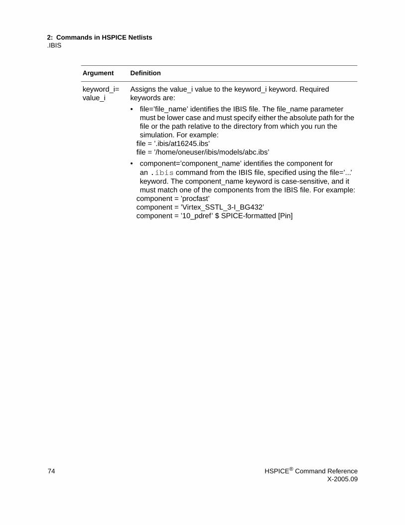
2: Commands in HSPICE Netlists.IBIS
keyword_i=value_i
Assigns the value_i value to the keyword_i keyword. Required keywords are:
• file=’file_name’ identifies the IBIS file. The file_name parameter must be lower case and must specify either the absolute path for the file or the path relative to the directory from which you run the simulation. For example:
file = ’.ibis/at16245.ibs’file = ’/home/oneuser/ibis/models/abc.ibs’
• component=’component_name’ identifies the component for an .ibis command from the IBIS file, specified using the file=’...’ keyword. The component_name keyword is case-sensitive, and it must match one of the components from the IBIS file. For example:
component = ’procfast’component = ’Virtex_SSTL_3-I_BG432’component = ’10_pdref’ $ SPICE-formatted [Pin]
Argument Definition
74 HSPICE® Command ReferenceX-2005.09

2: Commands in HSPICE Netlists.IBIS
See Also.EBD.PKG
keyword_m=value_m
Optional keywords:
• package = [0|1|2|3] (default is 3)• 0, does not add the rlc package into the component.• 1, adds [Package] (in .ibs file).• 2, adds [Pin] (in .ibs file).• 3, If [Package Model] is defined, set package with package model. If
it is not defined, set package with [Pin]. If the package information is not set in [Pin], set package with [Package] as a default. Package Model can be defined in either the IBIS file or the PKG file.
• The following optional keywords are the same as for the B Element (I/O buffer). For more information, see “Specifying Common Keywords” in the Modeling Input/Output Buffers Using IBIS chapter of the HSPICE Signal Integrity Guide.
• typ• interpo• ramp_rwf• ramp_fwf• rwf_tune• fwf_tune• pd_scal• pu_scal• pc_scal• gc_scal• rwf_scal• fwf_scal• nowarn• hsp_ver• c_com_pu• c_com_pd• c_com_pc• c_com_gc
Argument Definition
HSPICE® Command Reference 75X-2005.09

2: Commands in HSPICE Netlists.IC
.IC
Syntax.IC V(node1) = val1 V(node2) = val2 ...
Example.IC V(11) = 5 V(4) = -5 V(2) = 2.2
DescriptionUse the .IC statement or the .DCVOLT statement to set transient initial conditions in HSPICE, but not in HSPICE RF. How it initializes depends on whether the .TRAN analysis statement includes the UIC parameter.
Note: In HSPICE RF, .IC is always set to OFF.
If you specify the UIC parameter in the .TRAN statement, HSPICE does not calculate the initial DC operating point, but directly enters transient analysis. Transient analysis uses the .IC initialization values as part of the solution for timepoint zero (calculating the zero timepoint applies a fixed equivalent voltage source). The .IC statement is equivalent to specifying the IC parameter on each element statement, but is more convenient. You can still specify the IC parameter, but it does not have precedence over values set in the .IC statement.
If you do not specify the UIC parameter in the .TRAN statement, HSPICE computes the DC operating point solution before the transient analysis. The node voltages that you specify in the .IC statement are fixed to determine the DC operating point. HSPICE RF does not output node voltage from operating point (.OP), if time (t) < 0. Transient analysis releases the initialized nodes to calculate the second and later time points.
Argument Definition
val1 ... Specifies voltages. The significance of these voltages depends on whether you specify the UIC parameter in the .TRAN statement.
node1 ... Node numbers or names can include full paths or circuit numbers.
76 HSPICE® Command ReferenceX-2005.09

2: Commands in HSPICE Netlists.IC
See Also.DCVOLT.TRAN.OPTION DCIC
HSPICE® Command Reference 77X-2005.09

2: Commands in HSPICE Netlists.ICM
.ICM
Syntax.ICM icmname+ file = 'icmfilename'+ model = 'icmmodelname'
Example 1.ICM icm1+ file = 'test1.icm'+ model = 'FourLineModel1'
Example 2The following example shows how to reference a pin of ICM model in HSPICE netlist.
icm1_NodeMap1_pin1, icm1_NodeMap2_pin1,icm1_NodeMap2_pin2, ...
DescriptionThe .ICM command automatically creates port names that reference the pin name of an ICM model and generate a series of element (W/S/RLGCK) nodes on the pin when one of the following conditions occur:■ If the model is described using [Nodal Path Description]
'icmname'_'nodemapname'_'pinname'■ If the model is described using [Tree Path Description]
'icmname'_'pinmapname'_'pinname'
Argument Definition
icmname .ICM command card name.
icmfilename Name of an .icm file that contains an ICM model.
icmmodelname Working model in an .icm file.
nodemapname Name of the [ICM node map] keyword in an .icm file.
pinmapname Name of the [ICM pin map] keyword in an .icm file.
pinname Name of the first column of entries of the [ICM node map] or [ICM pin map].
78 HSPICE® Command ReferenceX-2005.09

2: Commands in HSPICE Netlists.IF
.IF
Syntax.IF (condition1)...<.ELSEIF (condition2)... > <.ELSE ... > .ENDIF
Example.IF (a==b).INCLUDE /myhome/subcircuits/diode_circuit1....ELSEIF (a==c).INCLUDE /myhome/subcircuits/diode_circuit2....ELSE.INCLUDE /myhome/subcircuits/diode_circuit3....ENDIF
DescriptionHSPICE executes the commands that follow the first.ELSEIF statement, only if condition1 in the preceding .IF statement is false, and condition2 in the first .ELSEIF statement is true.
If condition1 in the .IF statement and condition2 in the first .ELSEIF statement are both false, then HSPICE moves on to the next .ELSEIF statement, if there is one. If this second .ELSEIF condition is true, HSPICE executes the commands that follow the second .ELSEIF statement, instead of the commands after the first .ELSEIF statement.
HSPICE ignores the commands in all false .IF and .ELSEIF statements, until it reaches the first .ELSEIF condition that is true. If no .IF or .ELSEIF condition is true, HSPICE continues to the .ELSE statement
.ELSE precedes one or more commands in a conditional block, after the last .ELSEIF statement, but before the .ENDIF statement. HSPICE executes these commands by default, if the conditions in the preceding .IF statement, and in all of the preceding .ELSEIF statements in the same conditional block, are all false.
HSPICE® Command Reference 79X-2005.09

2: Commands in HSPICE Netlists.IF
The .ENDIF statement ends a conditional block of commands that begins with an .IF statement.
See Also.ELSE.ELSEIF.ENDIF
Argument Definition
condcition1 Condition that must be true, before HSPICE executes the commands that follow the .IF statement.
condition2 Condition that must be true, before HSPICE executes the commands that follow the .ELSEIF statement. HSPICE executes the commands that follow condition2, only if condition1 is false and condition2 is true.
80 HSPICE® Command ReferenceX-2005.09

2: Commands in HSPICE Netlists.INCLUDE
.INCLUDE
Syntax.INCLUDE ‘<filepath> filename’
Example.INCLUDE /myhome/subcircuits/diode_circuit
DescriptionYou can include a netlist as a subcircuit in one or more other netlists. To include another netlist in the current netlist, use the .INCLUDE statement.
Argument Definition
filepath Path name of a file for computer operating systems that support tree-structured directories.
A .INC file can contain nested .INC calls to itself or to another .INC file. If you use a relative path in a nested .INC call, the path starts from the directory of the parent .INC file, not from the work directory. If the path starts from the work directory, HSPICE can also find the .INC file, but prints a warning.
filename Name of a file to include in the data file. The file path, plus the file name, can be up to 1024 characters long. You can use any valid file name for the computer’s operating system. You must enclose the file path and name in single or double quotation marks.
HSPICE® Command Reference 81X-2005.09

2: Commands in HSPICE Netlists.LAYERSTACK
.LAYERSTACK
Syntax.LAYERSTACK sname <BACKGROUND=mname> + <LAYER=(mname,thickness) ...>
DescriptionA layer stack defines a stack of dielectric or metal layers.
You must associate each transmission line system with one, and only one, layer stack. However, you can associate a single-layer stack with many transmission line systems.
In the layer stack: ■ Layers are listed from bottom to top.■ Metal layers (ground planes) are located only at the bottom, only at the top,
or both at the top and bottom. ■ Layers are stacked in the y-direction, and the bottom of a layer stack is at
y=0. ■ All conductors must be located above y=0. ■ Background material must be dielectric.
The following limiting cases apply to the .LAYERSTACK command:■ Free space without ground:
.LAYERSTACK mystack
■ Free space with a (bottom) ground plane:.LAYERSTACK halfSpace PEC 0.1mm
Argument Definition
sname Layer stack name.
mname Material name.
BACKGROUND Background dielectric material name. By default, the Field Solver assumes AIR for the background.
thickness Layer thickness.
82 HSPICE® Command ReferenceX-2005.09

2: Commands in HSPICE Netlists.LAYERSTACK
See Also.FSOPTIONS.MATERIAL.SHAPE
HSPICE® Command Reference 83X-2005.09

2: Commands in HSPICE Netlists.LIB
.LIB
SyntaxUse the following syntax for library calls:
.LIB ‘<filepath> filename’ entryname
Use the following syntax to define library files:
.LIB entryname1
. $ ANY VALID SET OF HSPICE STATEMENTS
.ENDL entryname1
.LIB entryname2
.
. $ ANY VALID SET OF HSPICE STATEMENTS
.ENDL entryname2
.LIB entryname3
.
. $ ANY VALID ET OF HSPICE STATEMENTS
.ENDL entryname3
Example 1* Library call.LIB 'MODELS' cmos1
Example 2.LIB MOS7$ Any valid set of HSPICE commands....ENDL MOS7
Example 3The following are an illegal example and a legal example of nested .LIB statements for the file3 library.
Illegal:
.LIB MOS7
...
.LIB 'file3' MOS7 $ This call is illegal in MOS7 library
...
...
.ENDL
84 HSPICE® Command ReferenceX-2005.09

2: Commands in HSPICE Netlists.LIB
Legal:
.LIB MOS7
...
.LIB 'file1' MOS8
.LIB 'file2' MOS9
.LIB CTT $ file2 is already open for the CTT $ entry point
.ENDL
Example 4.LIB TT$TYPICAL P-CHANNEL AND N-CHANNEL CMOS LIBRARY$ PROCESS: 1.0U CMOS, FAB7$ following distributions are 3 sigma ABSOLUTE GAUSSIAN.PARAM TOX = AGAUSS(200,20,3) $ 200 angstrom +/- 20a+ XL = AGAUSS(0.1u,0.13u,3) $ polysilicon CD+ DELVTON = AGAUSS(0.0,.2V,3) $ n-ch threshold change+ DELVTOP = AGAUSS(0.0,.15V,3)
$ p-ch threshold change.INC ‘/usr/meta/lib/cmos1_mod.dat’
$ model include file.ENDL TT.LIB FF$HIGH GAIN P-CH AND N-CH CMOS LIBRARY 3SIGMA VALUES.PARAM TOX = 220 XL = -0.03 DELVTON = -.2V + DELVTOP = -0.15V.INC ‘/usr/meta/lib/cmos1_mod.dat’
$ model include file.ENDL FF
This example is a .LIB call statement of model skew parameters, and features both worst-case and statistical distribution data. The statistical distribution median value is the default for all non-Monte Carlo analysis. The model is in the /usr/meta/lib/cmos1_mod.dat include file.
.MODEL NCH NMOS LEVEL = 2 XL = XL TOX = TOX + DELVTO = DELVTON ......MODEL PCH PMOS LEVEL = 2 XL = XL TOX = TOX + DELVTO = DELVTOP .....
The .model keyword (left side) equates to the skew parameter (right side). A .model keyword can be the same as a skew parameter.
HSPICE® Command Reference 85X-2005.09
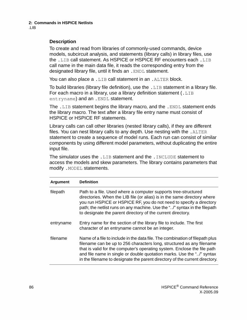
2: Commands in HSPICE Netlists.LIB
DescriptionTo create and read from libraries of commonly-used commands, device models, subcircuit analysis, and statements (library calls) in library files, use the .LIB call statement. As HSPICE or HSPICE RF encounters each .LIB call name in the main data file, it reads the corresponding entry from the designated library file, until it finds an .ENDL statement.
You can also place a .LIB call statement in an .ALTER block.
To build libraries (library file definition), use the .LIB statement in a library file. For each macro in a library, use a library definition statement (.LIB entryname) and an .ENDL statement.
The .LIB statement begins the library macro, and the .ENDL statement ends the library macro. The text after a library file entry name must consist of HSPICE or HSPICE RF statements.
Library calls can call other libraries (nested library calls), if they are different files. You can nest library calls to any depth. Use nesting with the .ALTER statement to create a sequence of model runs. Each run can consist of similar components by using different model parameters, without duplicating the entire input file.
The simulator uses the .LIB statement and the .INCLUDE statement to access the models and skew parameters. The library contains parameters that modify .MODEL statements.
Argument Definition
filepath Path to a file. Used where a computer supports tree-structured directories. When the LIB file (or alias) is in the same directory where you run HSPICE or HSPICE RF, you do not need to specify a directory path; the netlist runs on any machine. Use the “../” syntax in the filepath to designate the parent directory of the current directory.
entryname Entry name for the section of the library file to include. The first character of an entryname cannot be an integer.
filename Name of a file to include in the data file. The combination of filepath plus filename can be up to 256 characters long, structured as any filename that is valid for the computer’s operating system. Enclose the file path and file name in single or double quotation marks. Use the “../” syntax in the filename to designate the parent directory of the current directory.
86 HSPICE® Command ReferenceX-2005.09

2: Commands in HSPICE Netlists.LIB
See Also.ALTER
.ENDL
.INCLUDE
HSPICE® Command Reference 87X-2005.09

2: Commands in HSPICE Netlists.LIN
.LIN
Syntax.LIN <sparcalc = [1|0] <modelname = ...>> + <filename = ...> <format=[selem|citi|touchstone]>+ <noisecalc = [1|0] <gdcalc = [1|0]>+ <mixedmode2port = [dd|dc|ds|cd|cc|cs|sd|sc|ss]>+ <dataformat = [ri|ma|db]>
Example.LIN sparcalc=1 modelname=my_custom_model+ filename=mydesign format=touchstone noisecalc=1+ gdcalc=1 dataformat=ri
This example extracts linear transfer parameters for a general multi-port network, performs a 2-port noise analysis, and performs a group-delay analysis for a model named my_custom_model. The output is in the mydesign output file, which is in the TOUCHSTONE format. The data format in the TOUCHSTONE file is real-imaginary.
DescriptionThe .LIN command extracts noise and linear transfer parameters for a general multi-port network.
When used with P (port) element(s) and .AC commands, .LIN makes available a broad set of linear port-wise measurements:■ standard and mixed-mode multi-port S (scattering) parameters■ standard and mixed-mode multi-port Y/Z parameters■ standard mode multi-port H parameter ■ standard mode two-port noise parameters■ standard and mixed-mode group delays■ standard mode stability factors■ standard mode gain factors■ standard mode matching coefficients
The .LIN command computes the S (scattering), Y (admittance), Z (impedance) parameters directly, and H (hybrid) parameters directly based on the location of the port (P) elements in your circuit, and the specified values for their reference impedances.
88 HSPICE® Command ReferenceX-2005.09

2: Commands in HSPICE Netlists.LIN
The .LIN command also supports mixed-mode transfer parameters calculation and group delay analysis when used together with mixed-mode P elements.
By default, the .LIN command creates a .sc# file with the same base name as your netlist. This file contains S parameter, noise parameter, and group delay data as a function of the frequency. You can use this file as model data for the S element.
Argument Definition
sparcalc If 1, extract S parameters (default).
modelname Model name listed in the .MODEL statement in the .sc# model output file.
filename Output file name (default=netlist name).
format Output file format:
• selem is for S element .sc# format, which you can include in the netlist.
• citi is CITIfile format.• touchstone is TOUCHSTONE file format.
noisecalc If 1, extract noise parameters (perform 2-port noise analysis). Default=0.
gdcalc If 1, extract group delay (perform group delay analysis). Default=0.
HSPICE® Command Reference 89X-2005.09

2: Commands in HSPICE Netlists.LIN
mixedmode2port The mixedmode2port keyword describes the mixed-mode data map of output mixed mode S parameter matrix. The availability and default value for this keyword depends on the first two port (P element) configuration as follows:
• case 1: p1=p2=single (standard mode P element) available: ss default: ss
• case 2: p1=p2=balanced (mixed mode P element) available: dd, cd, dc, cc default: dd
• case 3: p1=balanced p2=single available: ds, cs default: ds
• case 4: p1=single p2=balanced available: sd, sc default: sd
dataformat The dataformat keyword describe the data format output to the .sc#/touchstone/citi file.
• dataformat=RI, real-imaginary. This is the default for.sc#/citi file.
• dataformat=MA, magnitude-phase. This is the default format for touchstone file.
• dataformat=DB, DB(magnitude)-phase.HSPICE uses six digits for both frequency andS Parameters in HSPICE generated data files (.sc#/touchstone/citifile). The number of digits for noise parameters are five in .sc# and touchstone files and six digits in citifiles.
Argument Definition
90 HSPICE® Command ReferenceX-2005.09

2: Commands in HSPICE Netlists.LOAD
.LOAD
Syntax.LOAD <FILE = load_file> <RUN = PREVIOUS | CURRENT>
Example 1.TITLE.SAVE FILE=design.ic.LOAD FILE=design.ic0
$load--design.ic0 save--design.ic0.alter... $load--none save--design.ic1.alter... $load--none save--design.ic2.end
This example loads a file name design.ic0, which you previously saved using a .SAVE command.
Example 2.TITLE.SAVE FILE=design.ic.LOAD FILE=design.ic RUN=PREVIOUS
$load--none save--design.ic0.alter... $load--design.ic0 save--design.ic1.alter... $load--design.ic1 save--design.ic2.end
Example 3.TITLE.SAVE FILE=design.ic.LOAD FILE=design.ic RUN=CURRENT
$load--design.ic0 save--design.ic0.alter... $load--design.ic1 save--design.ic1.alter... $load--design.ic2 save--design.ic2.end
DescriptionUse the .LOAD statement to input the contents of a file, that you stored using the .SAVE statement in HSPICE.
HSPICE® Command Reference 91X-2005.09

2: Commands in HSPICE Netlists.LOAD
Note: HSPICE RF does not support the .SAVE and .LOAD (save and restart) statements.
Files stored with the .SAVE statement contain operating point information for the point in the analysis at which you executed .SAVE.
Do not use the .LOAD command for concatenated netlist files.
See Also.ALTER.SAVE
Argument Definition
load_file Name of the file in which .SAVE saved an operating point for the circuit under simulation.The format of the file name is <design>.ic#. Default is <design>.ic0, where design is the root name of the design.
RUN= Used only outside of .ALTER statements in a netlist that contains .ALTER statements. The format of file name is <design>.ic.
PREVIOUS Each .ALTER run uses the saved operating point from the previous .ALTER run in the same simulation.
CURRENT Each .ALTER run uses the saved operating point from the current .ALTER run in the last simulation.
92 HSPICE® Command ReferenceX-2005.09

2: Commands in HSPICE Netlists.MACRO
.MACRO
In HSPICE RF, you cannot replicate output commands within subcircuit (subckt) definitions.
Syntax.MACRO subnam n1 <n2 n3 …> <parnam = val> .EOM
Example 1*FILE SUB2.SP TEST OF SUBCIRCUITS.OPTION LIST ACCT
V1 1 0 1.PARAM P5 = 5 P2 = 10.SUBCKT SUB1 1 2 P4 = 4
R1 1 0 P4R2 2 0 P5X1 1 2 SUB2 P6 = 7X2 1 2 SUB2
.ENDS*.MACRO SUB2 1 2 P6 = 11
R1 1 2 P6R2 2 0 P2
.EOMX1 1 2 SUB1 P4 = 6X2 3 4 SUB1 P6 = 15X3 3 4 SUB2
*.MODEL DA D CJA = CAJA CJP = CAJP VRB = -20 IS = 7.62E-18+ PHI = .5 EXA = .5 EXP = .33.PARAM CAJA = 2.535E-16 CAJP = 2.53E-16.END
The preceding example defines two subcircuits: SUB1 and SUB2. These are resistor divider networks, whose resistance values are parameters (variables). The X1, X2, and X3 statements call these subcircuits. Because the resistor values are different in each call, these three calls produce different subcircuits.
Example 2.SUBCKT Inv a y Strength = 3
Mp1 <MosPinList> pMosMod L = 1.2u W = ’Strength * 2u’Mn1 <MosPinList> nMosMod L = 1.2u W = ’Strength * 1u’
.ENDS
...
HSPICE® Command Reference 93X-2005.09

2: Commands in HSPICE Netlists.MACRO
xInv0 a y0 Inv $ Default devices: p device = 6u,$ n device = 3u
xInv1 a y1 Inv Strength = 5 $ p device = 10u, n device = 5uxInv2 a y2 Inv Strength = 1 $ p device = 2u, n device = 1u...
This example implements an inverter that uses a Strength parameter. By default, the inverter can drive three devices. Enter a new value for the Strength parameter in the element line to select larger or smaller inverters for the application.
DescriptionYou can create a subcircuit description for a commonly-used circuit, and include one or more references to the subcircuit in your netlist.
To define a subcircuit in your netlist, use the .MACRO statement. Use the .EOM statement to terminate a .MACRO statement.
Argument Definition
subnam Specifies a reference name for the subcircuit model call.
n1 … Node numbers for external reference; cannot be the ground node (zero). Any element nodes that are in the subcircuit, but are not in this list, are strictly local with three exceptions:
• Ground node (zero).• Nodes assigned using BULK = node in MOSFET or BJT models.• Nodes assigned using the .GLOBAL statement.
parnam A parameter name set to a value. Use only in the subcircuit. To override this value, assign it in the subcircuit call, or set a value in a .PARAM statement.
SubDefaultsList <SubParam1>=<Expression>[<SubParam2>=<Expression>...]
94 HSPICE® Command ReferenceX-2005.09

2: Commands in HSPICE Netlists.MACRO
See Also.ENDS.EOM.MACRO.SUBCKT
HSPICE® Command Reference 95X-2005.09
2: Commands in HSPICE Netlists.MALIAS
.MALIAS
Syntax.MALIAS model_name=alias_name1 <alias_name2 ...>
■ model_name is the model name defined in the .model card.■ alias_name1... is the alias that an instance (element) of the model
references.
Example*file: test malias statement.OPTION acct tnom=50 list gmin=1e-14 post.temp 0.0 25.tran .1 2vdd 2 0 pwl 0 -1 1 1d1 2 1 zend dtemp=25d2 1 0 zen dtemp=25* malias statements.malias zendef = zen zend* model definition.model zendef d (vj=.8 is=1e-16 ibv=1e-9 bv=6.0 rs=10+ tt=0.11n n=1.0 eg=1.11 m=.5 cjo=1pf tref=50).end
■ zendef is a diode model■ zen and zend are its aliases. ■ The zendef model points to both the zen and zend aliases.
DescriptionYou can use the .MALIAS statement to assign an alias (another name) to a diode, BJT, JFET, or MOSFET model that you defined in a .MODEL statement. You cannot use the .MALIAS statement in HSPICE RF.
.MALIAS differs from .ALIAS in two ways:■ A model can define the alias in an .ALIAS statement, but not the alias in
a .MALIAS statement. The .MALIAS statment applies to an element (an instance of the model), not to the model itself.
■ The .ALIAS command works only if you include .ALTER in the netlist. You can use .MALIAS without .ALTER.
96 HSPICE® Command ReferenceX-2005.09

2: Commands in HSPICE Netlists.MALIAS
You can use .MALIAS to alias to a model name that you defined in a .MODEL statement or to alias to a subcircuit name that you defined in a .SUBCKT statement. The syntax for .MALIAS is the same in either usage.
Note: Using .MALIAS in .ALTER blocks is not recommended or supported.
See Also.ALIAS
HSPICE® Command Reference 97X-2005.09

2: Commands in HSPICE Netlists.MATERIAL
.MATERIAL
Note: You cannot use the .MATERIAL statement in HSPICE RF.
Syntax.MATERIAL mname METAL|DIELECTRIC <ER=val> + <UR=val> <CONDUCTIVITY=val> <LOSSTANGENT=val>
DescriptionThe field solver assigns the following default values for metal: ■ CONDUCTIVITY = -1 (perfect conductor)■ ER = 1
■ UR = 1
PEC is a pre-defined metal name. You cannot redefine its default values.
The field solver assigns the following default values for dielectrics: ■ CONDUCTIVITY = 0 (lossless dielectric)■ LOSSTANGENT = 0 (lossless dielectric)■ ER = 1
■ UR = 1
AIR is a pre-defined dielectric name. You cannot redefine its default values.
Because the field solver does not currently support magnetic materials, it ignores UR values.
Argument Definition
mname Material name.
METAL|DIELECTRIC Material type: METAL or DIELECTRIC.
ER Dielectric constant (relative permittivity).
UR Relative permeability.
CONDUCTIVITY Static field conductivity of conductor or lossy dielectric (S/m).
LOSSTANGENTAlternating field loss tangent of dielectric (tan ).δ
98 HSPICE® Command ReferenceX-2005.09

2: Commands in HSPICE Netlists.MATERIAL
See Also.LAYERSTACK
HSPICE® Command Reference 99X-2005.09

2: Commands in HSPICE Netlists.MEASURE
.MEASURE
DescriptionUse the .MEASURE statement to modify information and to define the results of successive HSPICE or HSPICE RF simulations. The .MEASURE statement prints user-defined electrical specifications of a circuit. Optimization (HSPICE only) uses .MEASURE statements extensively. The specifications include:■ propagation■ delay■ rise time■ fall time■ peak-to-peak voltage■ minimum and maximum voltage over a specified period■ other user-defined variables
You can also use .MEASURE with either the error function (ERRfun) or GOAL parameter to optimize circuit component values (HSPICE only), and to curve-fit measured data to model parameters.
The .MEASURE statement can use several different formats, depending on the application. You can use it for either DC sweep, AC, or transient analyses.
See Also.AC.DC.DCMATCH.DOUT.GRAPH.OPTION MEASDGT.OPTION MEASFAIL.OPTION MEASFILE.OPTION MEASSORT.OPTION MEASOUT.PLOT.PRINT.PROBE.STIM.TRAN
100 HSPICE® Command ReferenceX-2005.09

2: Commands in HSPICE Netlists.MEASURE (Rise, Fall, and Delay Measurements)
.MEASURE (Rise, Fall, and Delay Measurements)
Syntax.MEASURE <DC | AC | TRAN> result TRIG … TARG …+ <GOAL = val> <MINVAL = val> <WEIGHT = val>
The input syntax for delay, rise time, and fall time in HSPICE RF is:
.MEASURE <TRAN > varname TRIG_SPEC TARG_SPEC
In this syntax, varname is the user-defined variable name for the measurement (the time difference between TRIG and TARG events). The input syntax of TRIG_SPEC and TARG_SPEC is:
TRIG var VAL = val < TD = td > < CROSS = c | LAST > + < RISE = r | LAST > < FALL = f | LAST >+ <TRIG AT = time>
TARG var VAL = val < TD = td > < CROSS = c | LAST > + < RISE = r | LAST > < FALL = f | LAST>+ <TRIG AT = time>
Example 1* Example of rise/fall/delay measurement.MEASURE TRAN tdlay TRIG V(1) VAL = 2.5 TD = 10n+ RISE = 2 TARG V(2) VAL = 2.5 FALL = 2
This example measures the propagation delay between nodes 1 and 2 for a transient analysis. HSPICE measures the delay from the second rising edge of the voltage at node 1 to the second falling edge of node 2. The measurement begins when the second rising voltage at node 1 is 2.5 V, and ends when the second falling voltage at node 2 is 2.5 V. The TD = 10n parameter counts the crossings, after 10 ns has elapsed. HSPICE prints results as tdlay = <value>.
Example 2.MEASURE TRAN riset TRIG I(Q1) VAL = 0.5m RISE = 3+ TARG I(Q1) VAL = 4.5m RISE = 3* Rise/fall/delay measure with TRIG and TARG specs.MEASURE pwidth TRIG AT = 10n TARG V(IN) VAL = 2.5 + CROSS = 3
HSPICE® Command Reference 101X-2005.09

2: Commands in HSPICE Netlists.MEASURE (Rise, Fall, and Delay Measurements)
In the last example, TRIG. AT = 10n starts measuring time at t = 10 ns in the transient analysis. The TARG parameters end time measurement when V(IN) = 2.5 V, on the third crossing. pwidth is the printed output variable.
If you use the .TRAN analysis statement with a .MEASURE statement, do not use a non-zero start time in .TRAN statement or the .MEASURE results might be incorrect.
Example 3.MEAS TRAN TDEL12 TRIG V(signal1) VAL='VDD/2'+ RISE=10 TARG V(signal2) VAL='VDD/2' RISE=1 TD=TRIG
This example shows a target that is delayed until the trigger time before the target counts the edges.
DescriptionUse the Rise, Fall, and Delay form of the .MEASURE statement to measure independent-variable (time, frequency, or any parameter or temperature) differential measurements such as rise time, fall time, slew rate, or any measurement that requires determining independent variable values. This format specifies TRIG and TARG substatements. These two statements specify the beginning and end of a voltage or current amplitude measurement.
Argument Definition
MEASURE Specifies measurements. You can abbreviate to MEAS.
result Name associated with the measured value in the HSPICE or HSPICE RF output. This example measures the independent variable, beginning at the trigger, and ending at the target:
• Transient analysis measures time.• AC analysis measures frequency.• DC analysis measures the DC sweep variable. If simulation reaches the target before the trigger activates, the resulting value is negative.
Do not use DC, TRAN, or AC as the result name.
TRIG… Identifies the beginning of trigger specifications.
102 HSPICE® Command ReferenceX-2005.09

2: Commands in HSPICE Netlists.MEASURE (Rise, Fall, and Delay Measurements)
TARG … Identifies the beginning of target specifications.The input syntax for delay, rise time, and fall time in HSPICE RF is:
.MEASURE < TRAN > varname TRIG_SPEC TARG_SPEC
varname is the user-defined variable name for the measurement, the time difference between TRIG and TARG events.
<DC | AC | TRAN> Specifies the analysis type of the measurement. If you omit this parameter, HSPICE or HSPICE RF uses the last analysis mode that you requested.
GOAL Specifies the desired measure value in ERR calculation for optimization. To calculate the error, the simulation uses the equation:
.
MINVAL If the absolute value of GOAL is less than MINVAL, the MINVAL replaces the GOAL value in the denominator of the ERRfun expression. Used only in ERR calculation for optimization. Default = 1.0e-12.
WEIGHT Multiplies the calculated error by the weight value. Used only in ERR calculation for optimization. Default = 1.0.
TRIG/TARG Parameter
Definition
TRIG Indicates the beginning of the trigger specification.
trig_val Value of trig_var, which increments the counter for crossings, rises, or falls, by one.
trig_var Specifies the name of the output variable, that determines the logical beginning of a measurement. If HSPICE or HSPICE RF reaches the target before the trigger activates, .MEASURE reports a negative value.
TARG Indicates the beginning of the target signal specification.
Argument Definition
ERRfun GOAL result–( ) GOAL⁄=
HSPICE® Command Reference 103X-2005.09

2: Commands in HSPICE Netlists.MEASURE (Rise, Fall, and Delay Measurements)
targ_val Specifies the value of the targ_var, which increments the counter for crossings, rises, or falls, by one.
targ_var Name of the output variable, at which HSPICE or HSPICE RF determines the propagation delay with respect to the trig_var.
time_delay Amount of simulation time that must elapse, before HSPICE or HSPICE RF enables the measurement. Simulation counts the number of crossings, rises, or falls, only after the time_delay value. Default trigger delay is zero.
TRIG/TARG Parameter
Definition
104 HSPICE® Command ReferenceX-2005.09

2: Commands in HSPICE Netlists.MEASURE (Average, RMS, and Peak Measurements)
.MEASURE (Average, RMS, and Peak Measurements)
Syntax.MEASURE <TRAN > out_var func var + FROM = start TO = end
Example 1.MEAS TRAN RMSVAL RMS V(OUT) FROM = 0NS TO = 10NS
In this example, the .MEASURE statement calculates the RMS voltage of the OUT node, from 0ns to 10ns. It then labels the result RMSVAL.
Example 2.MEAS MAXCUR MAX I(VDD) FROM = 10NS TO = 200NS
In this example, the .MEASURE statement finds the maximum current of the VDD voltage supply, between 10ns and 200ns in the simulation. The result is called MAXCUR.
Example 3.MEAS P2P PP PAR(‘V(OUT)/V(IN)’) + FROM = 0NS TO = 200NS
In this example, the .MEASURE statement uses the ratio of V(OUT) and V(IN) to find the peak-to-peak value in the interval of 0ns to 200ns.
DescriptionThis ..MEASURE statement reports the average, RMS, or peak value of the specified output variable.
HSPICE® Command Reference 105X-2005.09

2: Commands in HSPICE Netlists.MEASURE (Average, RMS, and Peak Measurements)
Argument Definition
varname User-defined variable name for the measurement.
func One of the following keywords:
• AVG: Average area under var, divided by the period of interest.
• MAX: Maximum value of var over the specified interval.
• MIN: Minimum value of var over the specified interval.
• PP: Peak-to-peak: reports the maximum value, minus the minimum of var over the specified interval.
• RMS: Root mean squared: calculates the square
root of the area under the var2 curve, dividedby the period of interest.
• INTEG: Integral of var over the specified period.
out_var
var
Name of the output variable, which can be either the node voltage or the branch current of the circuit. You can also use an expression, consisting of the node voltages or the branch current.
start Starting time of the measurement period.
end Ending time of the measurement period.
106 HSPICE® Command ReferenceX-2005.09

2: Commands in HSPICE Netlists.MEASURE (FIND and WHEN)
.MEASURE (FIND and WHEN)
Syntax.MEASURE <DC | AC | TRAN> result + WHEN out_var = val <TD = val> + < RISE = r | LAST > < FALL = f | LAST >+ < CROSS = c | LAST >+ <GOAL = val> <MINVAL = val> <WEIGHT = val>
.MEASURE <DC | AC | TRAN> result + WHEN out_var1 = out_var2 + < TD = val > < RISE = r | LAST > + < FALL = f | LAST > + < CROSS = c| LAST > <GOAL = val> + <MINVAL = val> <WEIGHT = val>
.MEASURE <DC | AC | TRAN> result FIND out_var1 + WHEN out_var2 = val < TD = val > + < RISE = r | LAST > + < FALL = f | LAST > < CROSS = c| LAST > + <GOAL = val> <MINVAL = val> <WEIGHT = val>
.MEASURE <DC | AC | TRAN> result FIND out_var1 + WHEN out_var2 = out_var3 <TD = val > + < RISE = r | LAST > < FALL = f | LAST > + <CROSS = c | LAST> <GOAL = val> + <MINVAL = val> <WEIGHT = val>
.MEASURE <DC | AC | TRAN> result FIND out_var1 + AT = val <GOAL = val> <MINVAL = val> + <WEIGHT = val>
.MEASURE DC result FIND <DCMATCH_TOTAL |+ DCMATCH(InstanceName)> AT = val
Example* MEASURE statement using FIND/WHEN.MEAS TRAN TRT FIND PAR(‘V(3)-V(4)’) + WHEN V(1)=PAR(‘V(2)/2’) RISE = LAST.MEAS STIME WHEN V(4) = 2.5 CROSS = 3
In this example, the first measurement, TRT, calculates the difference between V(3) and V(4) when V(1) is half the voltage of V(2) at the last rise event.
HSPICE® Command Reference 107X-2005.09

2: Commands in HSPICE Netlists.MEASURE (FIND and WHEN)
The second measurement, STIME, finds the time when V(4) is 2.5V at the third rise-fall event. A CROSS event is a rising or falling edge.
DescriptionThe FIND and WHEN functions of the .MEASURE statement specify to measure:■ Any independent variables (time, frequency, parameter).■ Any dependent variables (voltage or current, for example).■ Derivative of a dependent variable, if a specific event occurs.
Argument Definition
CROSS = cRISE = rFALL = f
Numbers indicate which CROSS, FALL, or RISE event to measure. For example:
.meas tran tdlay trig v(1) val=1.5 td=10n + rise=2 targ v(2) val=1.5 fall=2
In the above example, rise=2 specifies to measure the v(1) voltage, only on the first two rising edges of the waveform. The value of these first two rising edges is 1. However, trig v(1) val=1.5 indicates to trigger when the voltage on the rising edge voltage is 1.5, which never occurs on these first two rising edges. So the v(1) voltage measurement never finds a trigger.
• RISE = r, the WHEN condition is met, and measurement occurs after the designated signal has risen r rise times.
• FALL = f, measurement occurs when the designated signal has fallen f fall times.
A crossing is either a rise or a fall so for CROSS = c, measurement occurs when the designated signal has achieved a total of c crossing times as a result of either rising or falling.
For TARG, the LAST keyword specifies the last event.
108 HSPICE® Command ReferenceX-2005.09

2: Commands in HSPICE Netlists.MEASURE (FIND and WHEN)
LAST HSPICE or HSPICE RF measures when the last CROSS, FALL, or RISE event occurs.
• CROSS = LAST, measurement occurs the last time the WHEN condition is true for a rising or falling signal.
• FALL = LAST, measurement occurs the last time the WHEN condition is true for a falling signal.
• RISE = LAST, measurement occurs the last time the WHEN condition is true for a rising signal.
LAST is a reserved word; you cannot use it as a parameter name in the above .MEASURE statements.
AT = val Special case for trigger specification. val is:
• Time for TRAN analysis.• Frequency for AC analysis.• Parameter for DC analysis.• SweepValue from .DC mismatch analysis.The trigger determines where measurement takes place.
<DC | AC | TRAN> Analysis type for the measurement. If you omit this parameter, HSPICE or HSPICE RF assumes the last analysis type that you requested.
FIND Selects the FIND function.
GOAL Desired .MEASURE value. Optimization uses this value in ERR calculation. The following equation calculates the error:
.
In HSPICE RF output, you cannot apply .MEASURE to waveforms generated from another .MEASURE statement in a parameter sweep.
LAST Starts measurement at the last CROSS, FALL, or RISE event.
• For CROSS = LAST, measurement starts the last time the WHEN condition is true for either a rising or falling signal.
• For FALL = LAST, measurement starts the last time the WHEN condition is true for a falling signal.
• For RISE = LAST, measurement starts the last time the WHEN condition is true for a rising signal.
LAST is a reserved word. Do not use it as a parameter name in these .MEASURE statements.
Argument Definition
ERRfun GOAL result–( ) GOAL⁄=
HSPICE® Command Reference 109X-2005.09

2: Commands in HSPICE Netlists.MEASURE (FIND and WHEN)
MINVAL If the absolute value of GOAL is less than MINVAL, then MINVAL replaces the GOAL value in the denominator of the ERRfun expression. Used only in ERR calculation for optimization. Default = 1.0e-12.
out_var(1,2,3) These variables establish conditions that start a measurement.
result Name of a measured value in the HSPICE or HSPICE RF output.
TD Time at which measurement starts.
WEIGHT Multiplies the calculated error by the weight value. Used only in ERR calculation for optimization. Default = 1.0.
WHEN Selects the WHEN function.
DCMATCH(InstanceName)
.DCMATCH contribution from InstanceName.
DCMATCH_TOTAL .DCMATCH total output variation.
Argument Definition
110 HSPICE® Command ReferenceX-2005.09

2: Commands in HSPICE Netlists.MEASURE (Equation Evaluation/ Arithmetic Expression)
.MEASURE (Equation Evaluation/ Arithmetic Expression)
Syntax.MEASURE <DC | TRAN | AC> result PARAM = ’equation’ + <GOAL = val> <MINVAL = val>
.MEASURE TRAN varname PARAM = “expression”
Example.MEAS TRAN V3MAX MAX V(3) FROM 0NS TO 100NS.MEAS TRAN V2MIN MIN V(2) FROM 0NS TO 100NS.MEAS VARG PARAM = ‘(V2MIN + V3MAX)/2’
The first two measurements, V3MAX and V2MIN, set up the variables for the third .MEASURE statement.■ V3MAX is the maximum voltage of V(3) between 0ns and 100ns of the
simulation.■ V2MIN is the minimum voltage of V(2) during that same interval. ■ VARG is the mathematical average of the V3MAX and V2MIN measurements.
DescriptionUse the Equation Evaluation form of the .MEASURE statement to evaluate an equation, that is a function of the results of previous .MEASURE statements. The equation must not be a function of node voltages or branch currents.
The expression option is an arithmetic expression, that uses results from other prior .MEASURE statements.
Expressions used in arithmetic expression must not be a function of node voltages or branch currents. Expressions used in all other .MEASURE statements can contain either node voltages or branch currents, but must not use results from other .MEASURE statements.
HSPICE® Command Reference 111X-2005.09

2: Commands in HSPICE Netlists.MEASURE (Average, RMS, MIN, MAX, INTEG, and PP)
.MEASURE (Average, RMS, MIN, MAX, INTEG, and PP)
Syntax.MEASURE <DC | AC | TRAN> result func out_var + <FROM = val> <TO = val> <GOAL = val> + <MINVAL = val> <WEIGHT = val>
.MEASURE DC results <MAX> + <DCMATCH_TOTAL | DCMATCH(InstanceName)>
Example 1.MEAS TRAN avgval AVG V(10) FROM = 10ns TO = 55ns
This example calculates the average nodal voltage value for node 10, during the transient sweep, from the time 10 ns to 55 ns. It prints out the result as avgval.
Example 2.MEAS TRAN MAXVAL MAX V(1,2) FROM = 15ns TO = 100ns
This example finds the maximum voltage difference between nodes 1 and 2 for the time period from 15 ns to 100 ns.
Example 3.MEAS TRAN MINVAL MIN V(1,2) FROM = 15ns TO = 100ns.MEAS TRAN P2PVAL PP I(M1) FROM = 10ns TO = 100ns
DescriptionAverage (AVG), RMS, MIN, MAX, and peak-to-peak (PP) measurement modes report statistical functions of the output variable, rather than analysis values. ■ AVG calculates the area under an output variable, divided by the periods of
interest.■ RMS divides the square root of the area under the output variable square, by
the period of interest. ■ MIN reports the minimum value of the output function, over the specified
interval. ■ MAX reports the maximum value of the output function, over the specified
interval. ■ PP (peak-to-peak) reports the maximum value, minus the minimum value,
over the specified interval.
112 HSPICE® Command ReferenceX-2005.09

2: Commands in HSPICE Netlists.MEASURE (Average, RMS, MIN, MAX, INTEG, and PP)
AVG, RMS, and INTEG have no meaning in a DC data sweep so if you use them, HSPICE or HSPICE RF issues a warning message.
Argument Definition
<DC|AC|TRAN> Specifies the analysis type for the measurement. If you omit this parameter, HSPICE or HSPICE RF assumes the last analysis mode that you requested.
FROM Specifies the initial value for the func calculation. For transient analysis, this value is in units of time.
TO Specifies the end of the func calculation.
GOAL Specifies the .MEASURE value. Optimization uses this value for ERR calculation. This equation calculates the error:
In HSPICE RF simulation output, you cannot apply .MEASURE to waveforms generated from another .MEASURE statement in a parameter sweep.
func Indicates one of the measure statement types:
• AVG (average): Calculates the area under the out_var, divided by the periods of interest.
• MAX (maximum): Reports the maximum value of the out_var, over the specified interval.
• MIN (minimum): Reports the minimum value of the out_var, over the specified interval.
• PP (peak-to-peak): Reports the maximum value, minus the minimum value of the out_var, over the specified interval.
• RMS (root mean squared): Calculates the square root of the area under the out_var2 curve, divided by the period of interest.
result Name of the measured value in the output. The value is a function of the variable (out_var) and func.
out_var Name of any output variable whose function (func) the simulation measures.
WEIGHT Multiplies the calculated error, by the weight value. Used only in ERR calculation for optimization. Default = 1.0.
ERRfun GOAL result–( ) GOAL⁄=
HSPICE® Command Reference 113X-2005.09

2: Commands in HSPICE Netlists.MEASURE (Average, RMS, MIN, MAX, INTEG, and PP)
DCMATCH(InstanceName)
.DCMATCH contribution from InstanceName.
DCMATCH_TOTAL
.DCMATCH total output variation.
Argument Definition
114 HSPICE® Command ReferenceX-2005.09

2: Commands in HSPICE Netlists.MEASURE (Integral Function)
.MEASURE (Integral Function)
Syntax.MEASURE <DC | AC | TRAN> result INTEGRAL out_var + <FROM = val> <TO = val> <GOAL = val> + <MINVAL = val> <WEIGHT = val>
Example.MEAS TRAN charge INTEG I(cload) FROM = 10ns+ TO = 100ns
This example calculates the integral of I(cload), from 10 ns to 100 ns.
DescriptionThe INTEGRAL function reports the integral of an output variable, over a specified period.
The INTEGRAL function (with func), uses the same syntax as the average (AVG), RMS, MIN, MAX, and peak-to-peak (PP) measurement mode to defined the INTEGRAL (INTEG).
HSPICE® Command Reference 115X-2005.09

2: Commands in HSPICE Netlists.MEASURE (Derivative Function)
.MEASURE (Derivative Function)
Syntax.MEASURE <DC | AC | TRAN> result DERIVATIVE out_var + AT = val <GOAL = val> <MINVAL = val> + <WEIGHT = val>
.MEASURE <DC | AC | TRAN> result DERIVATIVE out_var + WHEN var2 = val <RISE = r | LAST> + <FALL = f | LAST> <CROSS = c | LAST> <TD = tdval> + <GOAL = goalval> <MINVAL = minval> + <WEIGHT = weightval>
.MEASURE <DC | AC | TRAN> result DERIVATIVE out_var + WHEN var2 = var3 <RISE = r | LAST> + <FALL = f | LAST> <CROSS = c | LAST> <TD = tdval> + <GOAL = goalval> <MINVAL = minval> + <WEIGHT = weightval>
Example 1.MEAS TRAN slew rate DERIV V(out) AT = 25ns
This example calculates the derivative of V(out), at 25 ns.
Example 2.MEAS TRAN slew DERIV v(1) WHEN v(1) = ’0.90*vdd’
This example calculates the derivative of v(1) when v(1) is equal to 0.9*vdd.
Example 3.MEAS AC delay DERIV ’VP(output)/360.0’ AT = 10khz
This example calculates the derivative of VP(output)/360.0 when the frequency is 10 kHz.
DescriptionThe DERIVATIVE function provides the derivative of:■ An output variable, at a specified time or frequency. ■ Any sweep variable, depending on the type of analysis.■ A specified output variable when some specific event occurs.
116 HSPICE® Command ReferenceX-2005.09

2: Commands in HSPICE Netlists.MEASURE (Derivative Function)
Argument Definition
AT = val Value of out_var, at which the derivative is found.
CROSS = c
RISE = r
FALL = f
The numbers indicate which occurrence of a CROSS, FALL, or RISE event starts a measurement.
• For RISE = r when the designated signal has risen r rise times, the WHEN condition is met, and measurement starts.
• For FALL = f, measurement starts when the designated signal has fallen f fall times.
A crossing is either a rise or a fall so for CROSS = c, measurement starts when the designated signal has achieved a total of c crossing times as a result of either rising or falling.
<DC|AC|TRAN> Specifies the analysis type to measure. If you omit this parameter, HSPICE or HSPICE RF assumes the last analysis mode that you requested.
DERIVATIVE Selects the derivative function. You can abbreviate to DERIV.
GOAL Specifies the desired .MEASURE value. Optimization uses this value for ERR calculation. This equation calculates the error:
In HSPICE RF output, you cannot apply .MEASURE to waveforms generated from another .MEASURE statement in a parameter sweep.
LAST Measures when the last CROSS, FALL, or RISE event occurs.
• CROSS = LAST, measures the last time the WHEN condition is true for a rising or falling signal.
• FALL = LAST, measures the last time WHEN is true for a falling signal.
• RISE = LAST, measures the last time WHEN is true for a rising signal.
LAST is a reserved word; do not use it as a parameter name in the above .MEASURE statements.
MINVAL If the absolute value of GOAL is less than MINVAL, MINVAL replaces the GOAL value in the denominator of the ERRfun expression. Used only in ERR calculation for optimization. Default = 1.0e-12.
ERRfun GOAL result–( ) GOAL⁄=
HSPICE® Command Reference 117X-2005.09

2: Commands in HSPICE Netlists.MEASURE (Derivative Function)
out_var Variable for which HSPICE or HSPICE RF finds the derivative.
result Name of the measured value in the output.
TD Identifies the time when measurement starts.
var(2,3) These variables establish conditions that start a measurement.
WEIGHT Multiplies the calculated error, between result and GOAL, by the weight value. Used only in ERR calculation for optimization. Default = 1.0.
WHEN Selects the WHEN function.
Argument Definition
118 HSPICE® Command ReferenceX-2005.09

2: Commands in HSPICE Netlists.MEASURE (Error Function)
.MEASURE (Error Function)
Syntax.MEASURE <DC | AC | TRAN> result + ERRfun meas_var calc_var + <MINVAL = val> < IGNORE | YMIN = val> + <YMAX = val> <WEIGHT = val> <FROM = val> + <TO = val>
DescriptionThe relative error function reports the relative difference between two output variables. You can use this format in optimization and curve-fitting of measured data. The relative error format specifies the variable to measure and calculate, from the .PARAM variable. To calculate the relative error between the two, HSPICE or HSPICE RF uses the ERR, ERR1, ERR2, or ERR3 functions. With this format, you can specify a group of parameters to vary to match the calculated value and the measured data.
Argument Definition
<DC|AC|TRAN> Specifies the analysis type for the measurement. If you omit this parameter, HSPICE or HSPICE RF assumes the last analysis mode that you requested.
result Name of the measured result in the output.
ERRfun ERRfun indicates which error function to use: ERR, ERR1, ERR2, or ERR3.
meas_var Name of any output variable or parameter in the data statement. M denotes the meas_var in the error equation.
calc_var Name of the simulated output variable or parameter in the .MEASURE statement to compare with meas_var. C is the calc_var in the error equation.
IGNOR|YMIN If the absolute value of meas_var is less than the IGNOR value, then the ERRfun calculation does not consider this point. Default = 1.0e-15.
HSPICE® Command Reference 119X-2005.09

2: Commands in HSPICE Netlists.MEASURE (Error Function)
FROM Specifies the beginning of the ERRfun calculation. For transient analysis, the from value is in units of time. Defaults to the first value of the sweep variable.
WEIGHT Multiplies the calculated error, by the weight value. Used only in ERR calculation for optimization. Default = 1.0.
YMAX If the absolute value of meas_var is greater than the YMAX value, then the ERRfun calculation does not consider this point. Default = 1.0e+15.
TO End of the ERRfun calculation. Default is last value of the sweep variable.
MINVAL If the absolute value of meas_var is less than MINVAL, MINVAL replaces the meas_var value in the denominator of the ERRfun expression. Used only in ERR calculation for optimization. Default = 1.0e-12.
Argument Definition
120 HSPICE® Command ReferenceX-2005.09
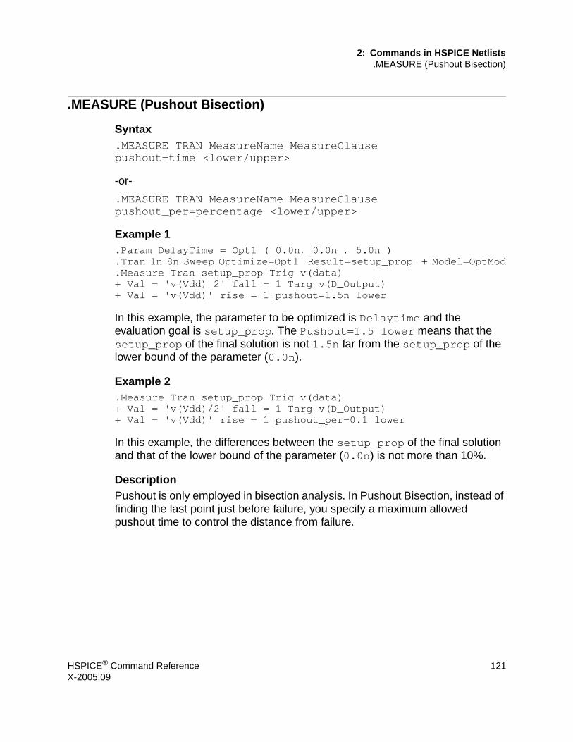
2: Commands in HSPICE Netlists.MEASURE (Pushout Bisection)
.MEASURE (Pushout Bisection)
Syntax.MEASURE TRAN MeasureName MeasureClausepushout=time <lower/upper>
-or-
.MEASURE TRAN MeasureName MeasureClause pushout_per=percentage <lower/upper>
Example 1.Param DelayTime = Opt1 ( 0.0n, 0.0n , 5.0n ).Tran 1n 8n Sweep Optimize=Opt1 Result=setup_prop + Model=OptMod.Measure Tran setup_prop Trig v(data)+ Val = 'v(Vdd) 2' fall = 1 Targ v(D_Output)+ Val = 'v(Vdd)' rise = 1 pushout=1.5n lower
In this example, the parameter to be optimized is Delaytime and the evaluation goal is setup_prop. The Pushout=1.5 lower means that the setup_prop of the final solution is not 1.5n far from the setup_prop of the lower bound of the parameter (0.0n).
Example 2.Measure Tran setup_prop Trig v(data)+ Val = 'v(Vdd)/2' fall = 1 Targ v(D_Output)+ Val = 'v(Vdd)' rise = 1 pushout_per=0.1 lower
In this example, the differences between the setup_prop of the final solution and that of the lower bound of the parameter (0.0n) is not more than 10%.
DescriptionPushout is only employed in bisection analysis. In Pushout Bisection, instead of finding the last point just before failure, you specify a maximum allowed pushout time to control the distance from failure.
HSPICE® Command Reference 121X-2005.09

2: Commands in HSPICE Netlists.MEASURE (Pushout Bisection)
Argument Definition
pushout=time Specifies the time. An appropriate time must be specified to obtain the pushout result (an absolute time).
pushout_per=percentage
Defines a relative error. If you specify a 0.1 relative error, the T_lower or T_upper and T_pushout have more than a 10% difference in value. This occurrence causes the iteration to stop and output the optimized parameter.
lower/upper Specifies the parameter boundary values for pushout comparison. These arguments are optional.
If the parameter is defined as .PARAM <ParamName>=OPTxxx(<Initial>, <min>. <max>), the "lower" means the lower bound "min”, and the “upper” means the upper bound "max". Default=lower.
122 HSPICE® Command ReferenceX-2005.09

2: Commands in HSPICE Netlists.MODEL
.MODEL
Syntax.MODEL mname type <VERSION = version_number>+ <pname1 = val1 pname2 = val2 ...>
.MODEL mname OPT <parameter=val ...>
The following is the .MODEL syntax for use with .GRAPH:
.MODEL mname PLOT (pnam1 = val1 pnam2 = val2….)
The following syntax is used for a Monte Carlo analysis:
.MODEL mname ModelType (<LEVEL=val>+ <keyname1=val1><keyname2=val2>+ <keyname3=val3><LOT</n></distribution>><value>+ <DEV</n></distribution>><value>...)+ <VERSION=version_number>
Example 1.MODEL MOD1 NPN BF=50 IS=1E-13 VBF=50 AREA=2 PJ=3, + N=1.05
Example 2This example shows a .MODEL statement used for a Monte Carlo analysis:
.model m1 nmos level=6 bulk=2 vt=0.7 dev/2 0.1+ tox=520 lot/gauss 0.3 a1=.5 a2=1.5 cdb=10e-16+ csb=10e-16 tcv=.0024
DescriptionUse the .MODEL command to include an instance (element) of a pre-defined HSPICE model in your input netlist.
For each optimization within a data file, specify a .MODEL statement. HSPICE can then execute more than one optimization per simulation run. The .MODEL optimization statement defines:■ Convergence criteria.■ Number of iterations.■ Derivative methods.
HSPICE® Command Reference 123X-2005.09

2: Commands in HSPICE Netlists.MODEL
Argument Definition
mname Model name reference. Elements must use this name to refer to the model.
If model names contain periods (.), the automatic model selector might fail.
When used with .GRAPH, this is the plot model name, referenced in .GRAPH statements.
type Selects a model type. Must be one of the following.
AMP operational amplifier model C capacitor model CORE magnetic core model D diode model L inductor model or magnetic core mutual
inductor model NJF n-channel JFET model NMOS n-channel MOSFET model NPN npn BJT model OPT optimization model PJF p-channel JFET model PLOT plot model for the .GRAPH statement PMOS p-channel MOSFET model PNP pnp BJT model R resistor modelU lossy transmission line model (lumped)W lossy transmission line model SP S parameter
124 HSPICE® Command ReferenceX-2005.09

2: Commands in HSPICE Netlists.MODEL
CENDIF Selects different derivative methods. Default=1.0e-9.
The following calculates the gradient of the RESULTS functions:
||Transpose(Jacobi(F(X))) * F(X)||, where F(X) is the RESULT function
If the resulting gradient is less than CENDIF, HSPICE uses more accurate but more time-consuming derivative methods. By default, HSPICE uses faster but less-accurate derivative methods. To use the more-accurate methods, set CENDIF to a larger value than GRAD.
If the gradient of the RESULTS function is less than GRAD, optimization finishes before CENDIF takes effect.
• If the value is too large, the optimizer requires more CPU time. • If the value is too small, the optimizer might not find as accurate an
answer.
CLOSE Initial estimate of how close parameter initial value estimates are to the solution. CLOSE multiplies changes in new parameter estimates. If you use a large CLOSE value, the optimizer takes large steps toward the solution. For a small value, the optimizer takes smaller steps toward the solution. You can use a smaller value for close parameter estimates, and a larger value for rough initial guesses. Default=1.0.
• If CLOSE is greater than 100, the steepest descent in the Levenburg-Marquardt algorithm dominates.
• If CLOSE is less than 1, the Gauss-Newton method dominates.For more details, see L. Spruiell, “Optimization Error Surfaces,” Meta-Software Journal, Volume 1, Number 4, December 1994.
CUT Modifies CLOSE, depending on how successful iterations are, toward the solution.
If the last iteration succeeds, descent toward the CLOSE solution decreases by the CUT value. That is, CLOSE = CLOSE / CUT
If the last iteration was not a successful descent to the solution, CLOSE increases by CUT squared. That is, CLOSE = CLOSE * CUT * CUT
CUT drives CLOSE up or down, depending on the relative success in finding the solution. The CUT value must be > 1. Default = 2.0.
DEV (Monte Carlo) DEV tolerance, which is independent (each device varies independently).
Argument Definition
HSPICE® Command Reference 125X-2005.09
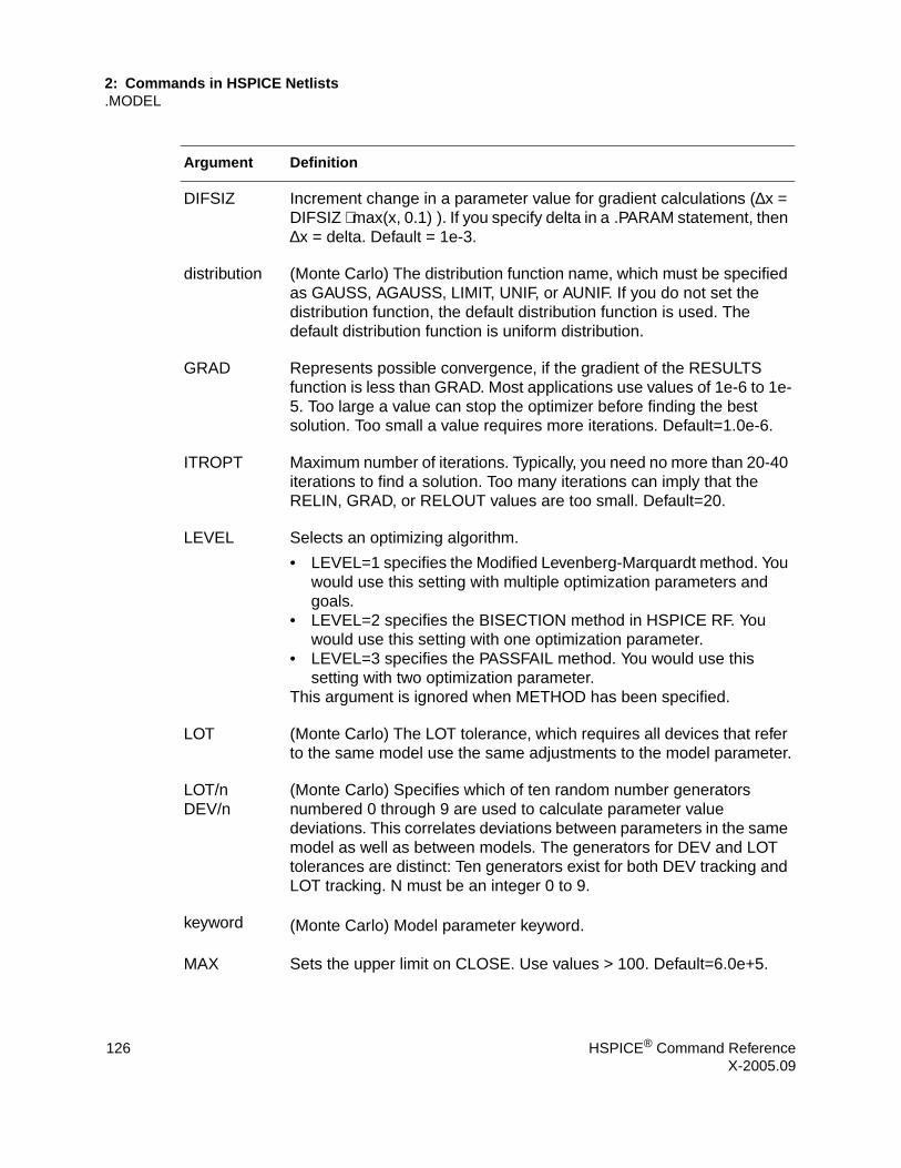
2: Commands in HSPICE Netlists.MODEL
DIFSIZ Increment change in a parameter value for gradient calculations (∆x = DIFSIZ ⋅ max(x, 0.1) ). If you specify delta in a .PARAM statement, then ∆x = delta. Default = 1e-3.
distribution (Monte Carlo) The distribution function name, which must be specified as GAUSS, AGAUSS, LIMIT, UNIF, or AUNIF. If you do not set the distribution function, the default distribution function is used. The default distribution function is uniform distribution.
GRAD Represents possible convergence, if the gradient of the RESULTS function is less than GRAD. Most applications use values of 1e-6 to 1e-5. Too large a value can stop the optimizer before finding the best solution. Too small a value requires more iterations. Default=1.0e-6.
ITROPT Maximum number of iterations. Typically, you need no more than 20-40 iterations to find a solution. Too many iterations can imply that the RELIN, GRAD, or RELOUT values are too small. Default=20.
LEVEL Selects an optimizing algorithm.
• LEVEL=1 specifies the Modified Levenberg-Marquardt method. You would use this setting with multiple optimization parameters and goals.
• LEVEL=2 specifies the BISECTION method in HSPICE RF. You would use this setting with one optimization parameter.
• LEVEL=3 specifies the PASSFAIL method. You would use this setting with two optimization parameter.
This argument is ignored when METHOD has been specified.
LOT (Monte Carlo) The LOT tolerance, which requires all devices that refer to the same model use the same adjustments to the model parameter.
LOT/nDEV/n
(Monte Carlo) Specifies which of ten random number generators numbered 0 through 9 are used to calculate parameter value deviations. This correlates deviations between parameters in the same model as well as between models. The generators for DEV and LOT tolerances are distinct: Ten generators exist for both DEV tracking and LOT tracking. N must be an integer 0 to 9.
keyword (Monte Carlo) Model parameter keyword.
MAX Sets the upper limit on CLOSE. Use values > 100. Default=6.0e+5.
Argument Definition
126 HSPICE® Command ReferenceX-2005.09

2: Commands in HSPICE Netlists.MODEL
METHOD Specifies an optimization method.
• METHOD = LM specifies the Modified Levenberg-Marquardt method.
• METHOD = BISECTION specifies the Bisection method. • METHOD = PASSFAIL specifies the Passfail method. This argument supersedes LEVEL when present.
PARMIN Allows better control of incremental parameter changes, during error calculations. Default=0.1. This produces more control over the trade-off between simulation time and optimization result accuracy. To calculate parameter increments, HSPICE uses the relationship:
Dpar_val = DIFSIZ ⋅ MAX(par_val, PARMIN)
PLOT A .GRAPH statement model.
pname1 ... Parameter name. Assign a model parameter name (pname1) from the parameter names for the appropriate model type. Each model section provides default values. For legibility, enclose the parameter assignment list in parentheses, and use either blanks or commas to separate each assignment. Use a plus sign (+) to start a continuation line.
When used with .GRAPH, each .GRAPH statement includes several model parameters. If you do not specify model parameters, HSPICE uses the default values of the model parameters, described in the following table. Pnamn is one of the model parameters of a .GRAPH statement, and valn is the value of pnamn. Valn can be more than one parameter.
RELIN Sets the relative input parameter (delta_par_val / MAX(par_val,1e-6)) for convergence. If all optimizing input parameters vary by no more than RELIN between iterations, the solution converges. RELIN is a relative variance test so a value of 0.001 implies that optimizing parameters vary by less than 0.1%, from one iteration to the next. Default=0.001.
RELOUT Sets the relative tolerance to finish optimization. For RELOUT=0.001, if the relative difference in the RESULTS functions, from one iteration to the next, is less than 0.001, then optimization is finished. Default=0.001.
Argument Definition
HSPICE® Command Reference 127X-2005.09

2: Commands in HSPICE Netlists.MODEL
VERSION HSPICE or HSPICE RF version number. Allows portability of the BSIM (LEVEL=13) and BSIM2 (LEVEL = 39) models, between HSPICE releases. HSPICE release numbers, and the corresponding version numbers, are:
HSPICE release Version number
9007B 9007.029007D 9007.0492A 92.0192B 92.0293A 93.0193A.02 93.0295.3 95.396.1 96.1
The VERSION parameter is valid only for LEVEL 13 and LEVEL 39 models. Use it with HSPICE Release H93A.02 and higher. If you use the parameter with any other model, or with a release before H93A.02, HSPICE issues a warning, but the simulation continues.You can also use VERSION to denote the BSIM3v3 version number only in model LEVELs 49 and 53. For LEVELs 49 and 53, the HSPVER parameter denotes the HSPICE or HSPICE RF release number.
Argument Definition
128 HSPICE® Command ReferenceX-2005.09
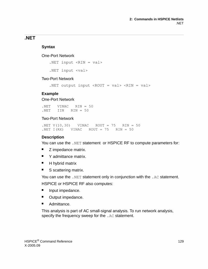
2: Commands in HSPICE Netlists.NET
.NET
Syntax
One-Port Network
.NET input <RIN = val>
.NET input <val>
Two-Port Network
.NET output input <ROUT = val> <RIN = val>
ExampleOne-Port Network
.NET VINAC RIN = 50
.NET IIN RIN = 50
Two-Port Network
.NET V(10,30) VINAC ROUT = 75 RIN = 50
.NET I(RX) VINAC ROUT = 75 RIN = 50
DescriptionYou can use the .NET statement or HSPICE RF to compute parameters for:■ Z impedance matrix.■ Y admittance matrix.■ H hybrid matrix■ S scattering matrix.
You can use the .NET statement only in conjunction with the .AC statement.
HSPICE or HSPICE RF also computes:■ Input impedance.■ Output impedance.■ Admittance.
This analysis is part of AC small-signal analysis. To run network analysis, specify the frequency sweep for the .AC statement.
HSPICE® Command Reference 129X-2005.09

2: Commands in HSPICE Netlists.NET
See Also.AC
Argument Definition
input Name of the voltage or current source for AC input.
output Output port. It can be:
• An output voltage, V(n1<,n2>).• An output current, I(source), or I(element).
RIN Input or source resistance. RIN calculates output impedance, output admittance, and scattering parameters. The default RIN value is 1 ohm.
ROUT Output or load resistance. ROUT calculates input impedance, admittance, and scattering parameters. Default=1 ohm.
130 HSPICE® Command ReferenceX-2005.09

2: Commands in HSPICE Netlists.NODESET
.NODESET
Syntax.NODESET V(node1) = val1 <V(node2) = val2 ...>
or
.NODESET node1 val1 <node2 val2>
Example.NODESET V(5:SETX) = 3.5V V(X1.X2.VINT) = 1V.NODESET V(12) = 4.5 V(4) = 2.23 .NODESET 12 4.5 4 2.23 1 1
DescriptionThe .NODESET statement initializes all specified nodal voltages for DC operating point analysis. Use the .NODESET statement to correct convergence problems in DC analysis. If you set the node values in the circuit close to the actual DC operating point solution, you enhance convergence of the simulation. The HSPICE or HSPICE RF simulator uses the NODESET voltages only in the first iteration to set an initial guess for DC operating point analysis.
See Also.DC
Argument Definition
node1 ... Node numbers or names can include full paths or circuit numbers.
val1 Specifies voltages.
HSPICE® Command Reference 131X-2005.09
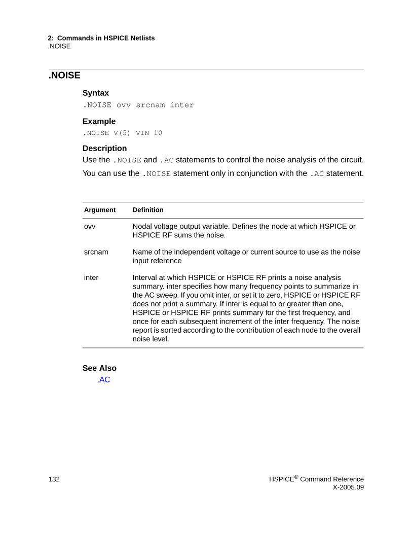
2: Commands in HSPICE Netlists.NOISE
.NOISE
Syntax.NOISE ovv srcnam inter
Example.NOISE V(5) VIN 10
DescriptionUse the .NOISE and .AC statements to control the noise analysis of the circuit.
You can use the .NOISE statement only in conjunction with the .AC statement.
See Also.AC
Argument Definition
ovv Nodal voltage output variable. Defines the node at which HSPICE or HSPICE RF sums the noise.
srcnam Name of the independent voltage or current source to use as the noise input reference
inter Interval at which HSPICE or HSPICE RF prints a noise analysis summary. inter specifies how many frequency points to summarize in the AC sweep. If you omit inter, or set it to zero, HSPICE or HSPICE RF does not print a summary. If inter is equal to or greater than one, HSPICE or HSPICE RF prints summary for the first frequency, and once for each subsequent increment of the inter frequency. The noise report is sorted according to the contribution of each node to the overall noise level.
132 HSPICE® Command ReferenceX-2005.09
2: Commands in HSPICE Netlists.OP
.OP
Syntax.OP <format> <time> <format> <time>... <interpolation>
Example 1.OP .5NS CUR 10NS VOL 17.5NS 20NS 25NS
This example calculates:■ Operating point at .05ns.■ Currents at 10 ns for the transient analysis.■ Voltages at 17.5 ns, 20 ns and 25 ns for the transient analysis.
Example 2.OP
This example calculates a complete DC operating point solution.
DescriptionWhen you include an .OP statement in an input file, HSPICE or HSPICE RF calculates the DC operating point of the circuit. You can also use the .OP statement to produce an operating point during a transient analysis. You can include only one .OP statement in a simulation.
If an analysis requires calculating an operating point, you do not need to specify the .OP statement; HSPICE or HSPICE RF calculates an operating point. If you use a .OP statement, and if you include the UIC parameter in a .TRAN analysis statement, then simulation omits the time = 0 operating point analysis, and issues a warning in the output listing.
HSPICE® Command Reference 133X-2005.09

2: Commands in HSPICE Netlists.OP
See Also.TRAN
Argument Definition
format Any of the following keywords. Only the first letter is required. Default = ALL
• ALL: Full operating point, including voltage, currents, conductances, and capacitances. This parameter outputs voltage/current for the specified time.
• BRIEF: Produces a one-line summary of each element’s voltage, current, and power. Current is stated in milliamperes, and power is in milliwatts.
• CURRENT: Voltage table with a brief summary of element currents and power.
• DEBUG: Usually invoked only if a simulation does not converge. Debug prints the non-convergent nodes, with the new voltage, old voltage, and the tolerance (degree of non-convergence). It also prints the non-convergent elements with their tolerance values.
• NONE: Inhibits node and element printouts, but performs additional analysis that you specify.
• VOLTAGE: Voltage table only.The preceding keywords are mutually-exclusive; use only one at a time.
time Place this parameter directly after ALL, VOLTAGE, CURRENT, or DEBUG. It specifies the time at which HSPICE or HSPICE RF prints the report. HSPICE RF returns node voltages only if time (t) is 0.
interpolation Selects the interpolation method for .OP time points during transient analysis, or no interpolation. Only the first character is required; that is, typing i has the same effect as typing interpolation. Default is not active.
If you specify interpolation, all of the time points in the .OP statement (except time=0) use the interpolation method to calculate the OP value during the transient analysis. If you use this keyword, it must be at the end of the .OP statement. HSPICE ignores any word after this keyword.
134 HSPICE® Command ReferenceX-2005.09

2: Commands in HSPICE Netlists.OPTION
.OPTION
Syntax.OPTION opt1 <opt2 opt3 ...>
Example.OPTION BRIEF $ Sets BRIEF to 1 (turns it on)* Netlist, models,....OPTION BRIEF = 0 $ Turns BRIEF off
This example sets the BRIEF option to 1 to suppress a printout. It then resets BRIEF to 0 later in the input file to resume the printout.
DescriptionYou use the .OPTION command to modify various aspects of a Synopsys HSPICE or HSPICE RF simulation, including:■ output types■ accuracy■ speed■ convergence
You can set any number of options in one .OPTION statement, and you can include any number of .OPTION statements in an input netlist file. Most options default to 0 (OFF) when you do not assign a value by using either .OPTION <opt> = <val> or the option with no assignment: .OPTION <opt>.
To reset options, set them to 0 (.OPTION <opt> = 0). To redefine an option, enter a new .OPTION statement; HSPICE or HSPICE RF uses the last definition.
You can use the following types of options with this command. For detailed information on individual options, see Chapter 3, Options in HSPICE Netlists.
Argument Definition
opt1 ... Specifies input control options. Many options are in the form <opt> = x, where <opt> is the option name and x is the value assigned to that option. Options are described in detail in Chapter 3, Options in HSPICE Netlists.
HSPICE® Command Reference 135X-2005.09

2: Commands in HSPICE Netlists.OPTION
■ General Control Options■ CPU Options■ Interface Options■ Analysis Options■ Error Options■ Version Option■ Model Analysis Options■ DC Operating Point, DC Sweep, and Pole/Zero Options■ Transient and AC Small Signal Analysis Options■ Transient Control Options■ Input/Output Options■ AC Control Options■ Common Model Interface Options■ Verilog-A Options
For instructions on how to use options that are relevant to a specific simulation type, see the appropriate DC, transient, and AC analysis chapters in the HSPICE Simulation and Analysis User Guide.
136 HSPICE® Command ReferenceX-2005.09

2: Commands in HSPICE Netlists.PARAM
.PARAM
Syntax
Simple parameter assignment:
.PARAM <ParamName>=<RealNumber>
Algebraic parameter assignments:
.PARAM <ParamName>=’<AlgebraicExpression>’
.PARAM <ParamName1>=<ParamName2>
User-defined functions:
.PARAM <ParamName>(<pv1>[<pv2>])=’<Expression>’
Pre-defined analysis functions:
.PARAM <FunctionName> = <Value>
Optimized parameter assignment:
.PARAM parameter=OPTxxx (initial_guess, low_limit, + upper_limit)
.PARAM parameter=OPTxxx (initial_guess, low_limit, + upper_limit, delta)
.PARAM <paramname>=str(‘string’)
Example 1* Simple parameter assignment.PARAM power_cylces=256
Example 2* Numerical parameter assignment.PARAM TermValue = 1g
rTerm Bit0 0 TermValuerTerm Bit1 0 TermValue
...
Example 3* Parameter assignment using expressions.PARAM Pi = ’355/113’.PARAM Pi2 = ’2*Pi’.PARAM npRatio = 2.1
HSPICE® Command Reference 137X-2005.09
2: Commands in HSPICE Netlists.PARAM
.PARAM nWidth = 3u
.PARAM pWidth = ’nWidth * npRatio’Mp1 ... <pModelName> W = pWidthMn1 ... <nModelName> W = nWidth...
Example 4* Algebraic parameter.param x=cos(2)+sin(2)
Example 5* Algebraic expression as an output variable.PRINT DC v(3) gain=PAR(‘v(3)/v(2)’) + PAR(‘V(4)/V(2)’)
Example 6* My own user-defined functions.PARAM <MyFunc( x, y )> = ‘Sqrt((x*x)+(y*y))’.PARAM CentToFar (c) = ’(((c*9)/5)+32)’.PARAM F(p1,p2) = ’Log(Cos(p1)*Sin(p2))’.PARAM SqrdProd (a,b) = ’(a*a)*(b*b)’
Example 7* Pre-defined analysis function.PARAM mcVar = Agauss(1.0,0.1)
Example 8.PARAM vtx=OPT1(.7,.3,1.0) uox=OPT1(650,400,900)
In this example, uox and vtx are the variable model parameters, which optimize a model for a selected set of electrical specifications.
The estimated initial value for the vtx parameter is 0.7 volts. You can vary this value within the limits of 0.3 and 1.0 volts for the optimization procedure. The optimization parameter reference name (OPT1) references the associated optimization analysis statement (not shown).
Example 9.PARAM fltmod = str('bpfmodel')s1 n1 n2 n3 n_ref fqmodel=fltmod zo=50 fbase=25e6 fmax=1e9
This example shows how you can define and use string parameters.
138 HSPICE® Command ReferenceX-2005.09

2: Commands in HSPICE Netlists.PARAM
Description
The .PARAM statement defines parameters. Parameters in HSPICE or HSPICE RF are names that have associated numeric values.
A parameter definition in HSPICE or HSPICE RF always uses the last value found in the input netlist (subject to local versus global parameter rules).
Use any of the following methods to define parameters:■ A simple parameter assignment is a constant real number. The parameter
keeps this value, unless a later definition changes its value, or an algebraic expression assigns a new value during simulation. HSPICE or HSPICE RF does not warn you if it reassigns a parameter.
■ An algebraic parameter (equation) is an algebraic expression of real values, a predefined or user-defined function, or circuit or model values. Enclose a complex expression in single quotes to invoke the algebraic processor, unless the expression begins with an alphabetic character and contains no spaces. A simple expression consists of a single parameter name. To use an algebraic expression as an output variable in a .PRINT, .PLOT, or .PROBE statement, use the PAR keyword or HSPICE RF (except that you cannot use the .PLOT statement in HSPICE RF).
■ A user-defined function assignment is similar to an algebraic parameter. HSPICE or HSPICE RF extends the algebraic parameter definition to include function parameters, used in the algebraic that defines the function. You can nest user-defined functions up to three deep.
■ A pre-defined analysis function. HSPICE or HSPICE RF provides several specialized analysis types, which require a way to control the analysis:
• Temperature functions (fn)
• Optimization guess/range
HSPICE also supports the following predefined parameter types, that HSPICE RF does not support:
• frequency
• time
• Monte Carlo functions
HSPICE® Command Reference 139X-2005.09

2: Commands in HSPICE Netlists.PARAM
Argument Definition
OPTxxx Optimization parameter reference name. The associated optimization analysis references this name. Must agree with the OPTxxx name in the analysis command associated with an OPTIMIZE keyname.
parameter Parameter to vary.
• Initial value estimate• Lower limit.• Upper limit. If the optimizer does not find the best solution within these constraints, it attempts to find the best solution without constraints.
delta The final parameter value is the initial guess ± (n⋅delta). If you do not specify delta, the final parameter value is between low_limit and upper_limit. For example, you can use this parameter to optimize transistor drawn widths and lengths, which must be quantized.
140 HSPICE® Command ReferenceX-2005.09

2: Commands in HSPICE Netlists.PAT
.PAT
Syntax.PAT <PatName>=data <RB=val> <R=repeat>
.PAT <patName>=[component 1 ... component n] <RB=val>+ <R=repeat>
Example 1The following example shows the .PAT command used for a b-string:
.PAT a1=b1010 r=1 rb=1
Example 2The following example shows how an existing patname is used to define a new patname:
.PAT a1=b1010 r=1 rb=1
.PAT a2=a1
Example 3This example shows a nested structure:
.PAT a1=[b1010 r=1 rb=2 b1100]
Example 4This final example shows how a predefined nested structure is used as a component in a new nested structure:
.PAT a1=[b1010 r=1 rb=2 b1100] r=1 rb=1
.PAT a2=[a1 b0m0m] r=2 rb=1
DescriptionWhen the .PAT command is used in an input file, some patnames are predefined and can be used in a pattern source. Patnames can associate a b-string or nested structure (NS), which are two different types of pattern sources. In this case, a b-string is a series of 1, 0, m, and z states. The NS is a combination of a b-string and another NS defined in the .PAT command. The .PAT command can also be used to define a new patname, which can be a b-string or NS.
You should avoid using a predefined patname to define another patname, which creates a circular definition. A circular definition is created when a patname is defined that depends on another patname, which in turn is defined
HSPICE® Command Reference 141X-2005.09

2: Commands in HSPICE Netlists.PAT
by the original patname. HSPICE detects circular definitions and issues an error report.
Nested structures must use brackets “[ ]”, but HSPICE does not support using multiple brackets in one statement. If you need to use another nested structure as a component in an NS, define the NS in a new .PAT command.
Argument Definition
data String of 1, 0, M, or Z that represents a pattern source. The first letter must be “B,” which represents it as a binary bit stream. This series is called b-string. A 1 represents the high voltage or current value, and a 0 is the low voltage or current value. An m represents the value which is equal to 0.5*(vhi+vlo), and a z represents the high impedance state (only for voltage source).
PatName Pattern name that has an associated b-string or nested structure.
component The elements that make up a nested structure. Components can be b-strings or a patnames defined in other .PAT commands.
RB=val Specifies the starting component of a repetition. The repeat data starts from the component or bit indicated by RB. RB must be an integer. If RB is larger than the length of the NS or b-string, an error is issued. If it is less than 1, it is automatically set to 1.
R=repeat Specifies how many times the repeating operation is executed. With no argument, the source repeats from the beginning of the NS or b-string. IfR=-1, the repeating operation continues forever. The R must be an integer. If it is less than -1, it automatically set to 0.
142 HSPICE® Command ReferenceX-2005.09

2: Commands in HSPICE Netlists.PKG
.PKG
Syntax.PKG pkgname +file= ’pkgfilename’ +model= ’pkgmodelname’
Example 1.pkg p_test+ file=’processor_clk_ff.ibs’+ model=’FCPGA_FF_PKG’
Example 2The following example shows how pin1 is referenced:
p_test_pin1_dia and p_test_pin1
The element name becomes:
w_p_test_pin1_?? or r_p_test_pin1_?? ...
DescriptionThe .PKG command provides the IBIS(V 3.2) Package Model feature. It supports both sections and matrixes.
The .PKG command automatically creates a series of elements (W or rlc). The following nodes are referenced in the netlist:■ Nodes on the die side:
’pkgname’_’pinname’_dia
■ Nodes on the pin side:
’pkgname’_’pinname’
See Example 2 for how pin1 is referenced.
Argument Definition
pkgname package card name
HSPICE® Command Reference 143X-2005.09

2: Commands in HSPICE Netlists.PKG
See Also.EBD.IBIS
pkgfilename name of a .pkg or .ibs file that contains package models.
pkgmodelname working model in the .pkg file
Argument Definition
144 HSPICE® Command ReferenceX-2005.09

2: Commands in HSPICE Netlists.PLOT
.PLOT
Note: This is an obsolete command. You can gain the same functionality by using the .PRINT command.
Syntax.PLOT antype ov1 <(plo1,phi1)> <ov2> <(plo2,phi2)> ...>
Example 1.PLOT DC V(4) V(5) V(1) PAR(`I1(Q1)/I2(Q1)').PLOT TRAN V(17,5) (2,5) I(VIN) V(17) (1,9).PLOT AC VM(5) VM(31,24) VDB(5) VP(5) INOISE
■ In the first line, PAR plots the ratio of the collector current and the base current for the Q1 transistor.
■ In the second line, the VDB output variable plots the AC analysis results (in decibels) for node 5.
■ In the third line, the AC plot can include NOISE results and other variables that you specify.
Example 2.PLOT AC ZIN YOUT(P) S11(DB) S12(M) Z11(R).PLOT DISTO HD2 HD3(R) SIM2.PLOT TRAN V(5,3) V(4) (0,5) V(7) (0,10).PLOT DC V(1) V(2) (0,0) V(3) V(4) (0,5)
In the last line above, HSPICE sets the plot limits for V(1) and V(2), but you specify 0 and 5 volts as the plot limits for V(3) and V(4).
DescriptionThe .PLOT statement plots the output values of one or more variables in a selected HSPICE analysis. Each .PLOT statement defines the contents of one plot, which can contain more than one output variable.
If more than one output variable appears on the same plot, HSPICE prints and plots the first variable specified. To print out more than one variable, include another .PLOT statement.
You can include wildcards in .PLOT statements (HSPICE only).
HSPICE® Command Reference 145X-2005.09

2: Commands in HSPICE Netlists.PLOT
See Also.AC.DOUT.GRAPH.MEASURE.PRINT.PROBE.STIM
Argument Definition
antype Type of analysis for the specified plots. Analysis types are: DC, AC, TRAN, NOISE, or DISTO.
ov1 … Output variables to plot: voltage, current, or element template variables (HSPICE only; HSPICE RF does not support element template output or .PLOT statements), from a DC, AC, TRAN, NOISE, or DISTO analysis. See the next sections for syntax.
plo1, phi1 … Lower and upper plot limits. The plot for each output variable uses the first set of plot limits, after the output variable name. Set a new plot limit for each output variable, after the first plot limit. For example to plot all output variables that use the same scale, specify one set of plot limits at the end of the .PLOT statement. If you set the plot limits to (0,0) HSPICE automatically sets the plot limits.
146 HSPICE® Command ReferenceX-2005.09
2: Commands in HSPICE Netlists.PRINT
Syntax.PRINT antype ov1 <ov2 … >
Example 1* CASE 1.print v(din) i(mxn18).dc vdin 0 5.0 0.05.tran 1ns 60ns* CASE 2.dc vdin 0 5.0 0.05.tran 1ns 60ns.print v(din) i(mxn18)* CASE 3.dc vdin 0 5.0 0.05.print v(din) i(mxn18).tran 1ns 60ns
■ If you replace the .PRINT statement with:
.print TRAN v(din) i(mnx)
then all three cases have identical .sw0 and .tr0 files.■ If you replace the .print statement with:
.print DC v(din) i(mnx)
then the .sw0 and .tr0 files are different.
Example 2.PRINT TRAN V (4) I(VIN) PAR(`V(OUT)/V(IN)')
This example prints the results of a transient analysis for the nodal voltage named 4. It also prints the current through the voltage source named VIN. It also prints the ratio of the nodal voltage at the OUT and IN nodes.
Example 3.PRINT AC VM(4,2) VR(7) VP(8,3) II(R1)
■ Depending on the value of the ACOUT option, VM(4,2) prints the AC magnitude of the voltage difference, or the difference of the voltage magnitudes, between nodes 4 and 2.
■ VR(7) prints the real part of the AC voltage, between node 7 and ground.
HSPICE® Command Reference 147X-2005.09

2: Commands in HSPICE Netlists.PRINT
■ Depending on the ACOUT value, VP(8,3) prints the phase of the voltage difference between nodes 8 and 3, or the difference of the phase of voltage at node 8 and voltage at node 3.
■ II(R1) prints the imaginary part of the current, through R1.
Example 4.PRINT AC ZIN YOUT(P) S11(DB) S12(M) Z11(R)
This example prints:■ The magnitude of the input impedance.■ The phase of the output admittance.■ Several S and Z parameters.
This statement accompanies a network analysis by using the .AC and .NET analysis statements.
Example 5.PRINT DC V(2) I(VSRC) V(23,17) I1(R1) I1(M1)
This example prints the DC analysis results for several different nodal voltages and currents, through:■ The resistor named R1.■ The voltage source named VSRC.■ The drain-to-source current of the MOSFET named M1.
Example 6.PRINT NOISE INOISE
This example prints the equivalent input noise.
Example 7.PRINT DISTO HD3 SIM2(DB)
This example prints the magnitude of third-order harmonic distortion, and the decibel value of the intermodulation distortion sum, through the load resistor that you specify in the .DISTO statement (HSPICE only; not supported in HSPICE RF).
Example 8.PRINT AC INOISE ONOISE VM(OUT) HD3
148 HSPICE® Command ReferenceX-2005.09

2: Commands in HSPICE Netlists.PRINT
This statement includes NOISE, DISTO, and AC output variables in the same .PRINT statement in HSPICE. HSPICE RF supports NOISE and AC analysis, but not DISTO.
Example 9.PRINT pj1 = par(‘p(rd) +p(rs)‘)
This statement prints the value of pj1 with the specified function.
HSPICE or HSPICE RF ignores .PRINT statement references to nonexistent netlist part names, and prints those names in a warning.
Example 10Derivative function:
.PRINT der=deriv('v(NodeX)')
Integrate function:
.PRINT int = integ('v(NodeX)')
The parameter can be a node voltage, or a reasonable expression.
Example 11.print p1 = 3.print p2 = par("p1*5")
You can use p1 and p2 as parameters in netlist. The p1 value is 3; the p2 value is 15.
DescriptionThe .PRINT statement specifies output variables for which HSPICE or HSPICE RF prints values. You can include wildcards in .PRINT statements.
You can also use the iall keyword in a .PRINT statement to print all branch currents of all diode, BJT, JFET, or MOSFET elements in your circuit design.
HSPICE® Command Reference 149X-2005.09

2: Commands in HSPICE Netlists.PRINT
See Also
.AC
.DC
.OPTION ACOUT
.DISTO
.DOUT
.GRAPH
.MEASURE
.NOISE
.PLOT
.PROBE
.STIM
.TRAN
Argument Definition
antype Type of analysis for outputs. Antype is one of the following types: DC, AC, TRAN, NOISE, or DISTO (you cannot run DISTO analysis in HSPICE RF).
ov1 … Output variables to print. These are voltage, current, or element template (HSPICE only; HSPICE RF does not support element template output) variables, from a DC, AC, TRAN, NOISE, or DISTO analysis (you cannot run DISTO analysis in HSPICE RF).
150 HSPICE® Command ReferenceX-2005.09

2: Commands in HSPICE Netlists.PROBE
.PROBE
Syntax.PROBE antype ov1 <ov2 ...>
Example 1.PROBE DC V(4) V(5) V(1) beta = PAR(`I1(Q1)/I2(Q1)')
Example 2* Derivative function.PROBE der=deriv('v(NodeX)')* Integrate function.PROBE int = integ('v(NodeX)')
DescriptionThe .PROBE statement saves output variables into interface and graph data files.The parameter can be a node voltage, or a reasonable expression. You can include wildcards in .PROBE statements.
Argument Definition
antype Type of analysis for the specified plots. Analysis types are: DC, AC, TRAN, NOISE, or DISTO (you cannot run DISTO analysis in HSPICE RF).
ov1 … Output variables to plot: voltage, current, or element template (HSPICE only; HSPICE RF does not support element template output) variables from a DC, DCMATCH, AC, TRAN, NOISE, or DISTO analysis (you cannot run DISTO analysis in HSPICE RF). .PROBE can include more than one output variable.
HSPICE® Command Reference 151X-2005.09

2: Commands in HSPICE Netlists.PROBE
See Also.AC.DC.DCMATCH.DISTO.DOUT.GRAPH.MEASURE.NOISE.PLOT.PRINT.STIM.TRAN
152 HSPICE® Command ReferenceX-2005.09

2: Commands in HSPICE Netlists.PROTECT
.PROTECT
Syntax.PROTECT
DescriptionThe .PROTECT statement keeps models and cell libraries private. HSPICE RF does not support the .PROTECT statement. ■ The .PROTECT statement suppresses printing text from the list file, such as
when you use the BRIEF option.■ The .UNPROTECT command restores normal output functions.■ Any elements and models located between a .PROTECT and
an .UNPROTECT statement, inhibit the element and model listing from the LIST option.
■ The .OPTION NODE nodal cross reference, and the .OP operating point printout, do not list any nodes that are contained within the .PROTECT and .UNPROTECT statements.
See Also.UNPROTECT
HSPICE® Command Reference 153X-2005.09

2: Commands in HSPICE Netlists.PZ
.PZ
Syntax.PZ output input
.PZ ov srcname
Example.PZ V(10) VIN.PZ I(RL) ISORC
■ In the first pole/zero analysis, the output is the voltage for node 10, and the input is the VIN independent voltage source.
■ In the second pole/zero analysis, the output is the branch current for the RL branch, and the input is the ISORC independent current source.
DescriptionThe .PZ command performs pole/zero analysis (you do not need to specify .OP, because the simulator automatically invokes an operating point calculation). See “Pole/Zero Analysis” in the HSPICE Applications Manual for complete information about pole/zero analysis.
For a description of pole/zero options, see Chapter 3, Options in HSPICE Netlists.
.
Argument Definition
input Input source. Can be the name of any independent voltage or current source.
output Output variables, which can be:
• Any node voltage, V(n).• Any branch current, I(branch_name).
154 HSPICE® Command ReferenceX-2005.09

2: Commands in HSPICE Netlists.PZ
See Also.DC
ov Output variable:
• a node voltage V(n), or • a branch current I(element)
srcnam Input source:
• an independent voltage or • a current source name
Argument Definition
HSPICE® Command Reference 155X-2005.09

2: Commands in HSPICE Netlists.SAMPLE
.SAMPLE
Syntax.SAMPLE FS = freq <TOL = val> <NUMF = val> + <MAXFLD = val> <BETA = val>
DescriptionTo acquire data from analog signals, use the .SAMPLE statement with the .NOISE and .AC statements to analyze data sampling noise in HSPICE or HSPICE RF. The SAMPLE analysis performs a noise-folding analysis, at the output node.
.
See Also.AC.NOISE
Argument Definition
FS = freq Sample frequency in hertz.
TOL Sampling-error tolerance: the ratio of the noise power (in the highest folding interval) to the noise power (in baseband). Default = 1.0e-3.
NUMF Maximum number of frequencies that you can specify. The algorithm requires about ten times this number of internally-generated frequencies so keep this value small. Default = 100.
MAXFLD Maximum number of folding intervals (default = 10.0). The highest frequency (in hertz) that you can specify is: FMAX = MAXFLD ⋅ FS
BETA Optional noise integrator (duty cycle), at the sampling node:
• BETA = 0 no integrator• BETA = 1 simple integrator (default)If you clock the integrator (integrates during a fraction of the 1/FS sampling interval), then set BETA to the duty cycle of the integrator.
156 HSPICE® Command ReferenceX-2005.09

2: Commands in HSPICE Netlists.SAVE
.SAVE
Syntax.SAVE <TYPE = type_keyword> <FILE = save_file>+ <LEVEL = level_keyword> <TIME = save_time>
Example.TEMP -25 0 25.SAVE TYPE=NODESET FILE=my_design.ic0 LEVEL=ALL + TIME=0
This example saves the operating point corresponding to .TEMP -25 to a file named my_design.ic0.
DescriptionThe .SAVE statement in HSPICE stores the operating point of a circuit in a file that you specify. HSPICE RF does not support the .SAVE statement. For quick DC convergence in subsequent simulations, use the .LOAD statement to input the contents of this file. HSPICE saves the operating point by default, even if the HSPICE input file does not contain a .SAVE statement. To not save the operating point, specify .SAVE LEVEL = NONE.
You can save the operating point data as either an .IC or a .NODESET statement.
A parameter or temperature sweep saves only the first operating point.
.
Argument Definition
type_keyword Storage method for saving the operating point. The type can be one of the following. Default is NODESET.
• .NODESET: Stores the operating point as a .NODESET statement. Later simulations initialize all node voltages to these values, if you use the .LOAD statement. If circuit conditions change incrementally, DC converges within a few iterations.
• .IC: Stores the operating point as a .IC statement. Later simulations initialize node voltages to these values if the netlist includes the .LOAD statements.
save_file Name of the file that stores DC operating point data. The file name format is <design>.ic#. Default is <design>.ic0.
HSPICE® Command Reference 157X-2005.09

2: Commands in HSPICE Netlists.SAVE
See Also.IC.LOAD.NODESET
level_keyword Circuit level, at which you save the operating point. The level can be one of the following.
• ALL (default): Saves all nodes, from the top to the lowest circuit level. This option offers the greatest improvement in simulation time.
• TOP: Saves only nodes in the top-level design. Does not save subcircuit nodes.
• NONE: Does not save the operating point.
save_time Time during transient analysis when HSPICE saves the operating point. HSPICE requires a valid transient analysis statement to save a DC operating point. Default = 0.
Argument Definition
158 HSPICE® Command ReferenceX-2005.09
2: Commands in HSPICE Netlists.SENS
.SENS
Syntax.SENS ov1 <ov2 ...>
Example.SENS V(9) V(4,3) V(17) I(VCC)
DescriptionThe .SENS command obtains DC small-signal sensitivities of output variables for circuit parameters. You can use this command HSPICE, but not in HSPICE RF.
If the input file includes a .SENS statement, HSPICE determines DC small-signal sensitivities for each specified output variable, relative to every circuit parameter. The sensitivity measurement is the partial derivative of each output variable for a specified circuit element, measured at the operating point, and normalized to the total change in output magnitude. Therefore, the sum of the sensitivities of all elements is 100%. DC small-signal sensitivities are calculated for:■ resistors■ voltage sources■ current sources■ diodes■ BJTs (including Level 4, the VBIC95 model)■ MOSFETs (Level49 and Level53, Version=3.22).
You can perform only one .SENS analysis per simulation. Only the last .SENS statement is used in case more than one in present. The others are discarded with warnings.
The amount of output generated from a .SENS analysis is dependent on the size of the circuit.
.
Argument Definition
ov1 ov2 ... Branch currents, or nodal voltage for DC component-sensitivity analysis
HSPICE® Command Reference 159X-2005.09

2: Commands in HSPICE Netlists.SENS
See Also.DC
160 HSPICE® Command ReferenceX-2005.09

2: Commands in HSPICE Netlists.SHAPE
.SHAPE
Syntax.SHAPE sname Shape_Descriptor
DescriptionUse the .SHAPE statement to define a shape. The Field Solver uses the shape to describe a cross-section of the conductor.
See Also.FSOPTIONS.LAYERSTACK.MATERIAL
Argument Definition
sname Shape name.
Shape_Descriptor One of the following:
• Rectangle• Circle• Strip• Polygon
HSPICE® Command Reference 161X-2005.09
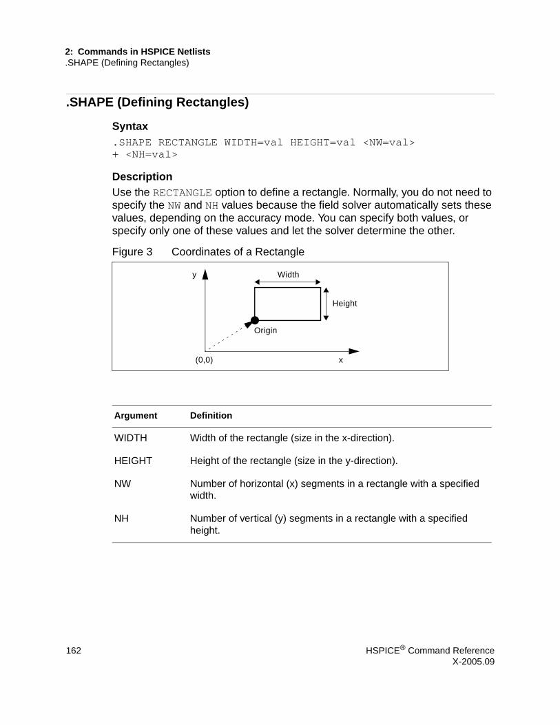
2: Commands in HSPICE Netlists.SHAPE (Defining Rectangles)
.SHAPE (Defining Rectangles)
Syntax.SHAPE RECTANGLE WIDTH=val HEIGHT=val <NW=val> + <NH=val>
DescriptionUse the RECTANGLE option to define a rectangle. Normally, you do not need to specify the NW and NH values because the field solver automatically sets these values, depending on the accuracy mode. You can specify both values, or specify only one of these values and let the solver determine the other.
Figure 3 Coordinates of a Rectangle
Argument Definition
WIDTH Width of the rectangle (size in the x-direction).
HEIGHT Height of the rectangle (size in the y-direction).
NW Number of horizontal (x) segments in a rectangle with a specified width.
NH Number of vertical (y) segments in a rectangle with a specified height.
(0,0)
Origin
Width
Height
x
y
162 HSPICE® Command ReferenceX-2005.09
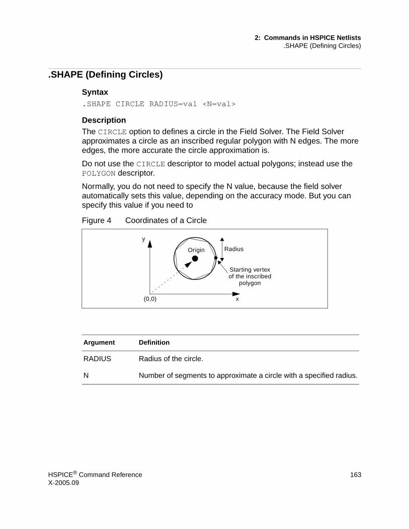
2: Commands in HSPICE Netlists.SHAPE (Defining Circles)
.SHAPE (Defining Circles)
Syntax.SHAPE CIRCLE RADIUS=val <N=val>
DescriptionThe CIRCLE option to defines a circle in the Field Solver. The Field Solver approximates a circle as an inscribed regular polygon with N edges. The more edges, the more accurate the circle approximation is.
Do not use the CIRCLE descriptor to model actual polygons; instead use the POLYGON descriptor.
Normally, you do not need to specify the N value, because the field solver automatically sets this value, depending on the accuracy mode. But you can specify this value if you need to
Figure 4 Coordinates of a Circle
Argument Definition
RADIUS Radius of the circle.
N Number of segments to approximate a circle with a specified radius.
(0,0)
Origin Radius
x
y
Starting vertexof the inscribed
polygon
HSPICE® Command Reference 163X-2005.09

2: Commands in HSPICE Netlists.SHAPE (Defining Polygons)
.SHAPE (Defining Polygons)
Syntax.SHAPE POLYGON VERTEX=(x1 y1 x2 y2 ...)+ <N=(n1,n2,...)>
Example 1The following rectangular polygon uses the default number of segments:
.SHAPE POLYGON VERTEX=(1 10 1 11 5 11 5 10)
Example 2The following rectangular polygon uses five segments for each edge:
.SHAPE POLYGON VERTEX=(1 10 1 11 5 11 5 10) + N=5
Example 3Rectangular polygon by using the different number of segments for each edge:
.SHAPE POLYGON VERTEX=(1 10 1 11 5 11 5 10) + N=(5 3 5 3)
DescriptionThe .SHAPE POLYGON command option defines a polygon in a Field Solver. The specified coordinates are within the local coordinate with respect to the origin of a conductor.
Figure 5 Coordinates of a Polygon
(0,0)
Origin
x
y
164 HSPICE® Command ReferenceX-2005.09

2: Commands in HSPICE Netlists.SHAPE (Defining Polygons)
Argument Definition
VERTEX (x, y) coordinates of vertices. Listed either in clockwise or counter-clockwise direction.
N Number of segments that define the polygon with the specified X and Y coordinates. You can specify a different N value for each edge. If you specify only one N value, then the Field Solver uses this value for all edges.
For example, the first value of N, n1, corresponds to the number of segments for the edge from (x1 y1) to (x2 y2).
HSPICE® Command Reference 165X-2005.09

2: Commands in HSPICE Netlists.SHAPE (Defining Strip Polygons)
.SHAPE (Defining Strip Polygons)
Syntax.SHAPE STRIP WIDTH=val <N=val>
DescriptionNormally, you do not need to specify the N value, because the field solver automatically sets this value, depending on the accuracy mode. But you can specify this value if you need to.
The field solver (filament method) does not support this shape.
Figure 6 Coordinates of a Strip Polygon
Argument Definition
WIDTH Width of the strip (size in the x-direction).
N Number of segments that define the strip shape with the specified width.
(0,0)
Origin
Width
x
y
166 HSPICE® Command ReferenceX-2005.09

2: Commands in HSPICE Netlists.STIM
.STIM
Syntax
General
.STIM <tran|ac|dc> PWL|DATA|VEC + <filename=output_filename> ...
PWL Source (Transient Analysis Only)
.STIM [tran] PWL [filename=output_filename] + [name1=] ovar1 [node1=n+] [node2=n-]+ [[name2=]ovar2 [node1=n+] [node2=n-] ...]+ [from=val] [to=val] [npoints=val]
.STIM [tran] PWL [filename=output_filename] + [name1=] ovar1 [node1=n+] [node2=n-]+ [[name2=]ovar2 [node1=n+] [node2=n-] ...]+ indepvar=[(]t1 [t2 ...[)]]
Data Card
.STIM [tran | ac | dc] DATA [filename=output_filename] + dataname [name1=] ovar1+ [[name2=]ovar2 ...] [from= val] [to=val]+ [npoints=val] [indepout=val]
.STIM [tran | ac | dc] DATA [filename=output_filename] + dataname [name1=] ovar1+ [[name2=]ovar2 ...] indepvar=[(]t1 [t2 ...[)]]+ [indepout=val]
Digital Vector File (Transient Analysis Only)
.STIM [tran] VEC [filename=output_filename] + vth=val vtl=val [voh=val] [vol=val] + [name1=] ovar1 [[name2=] ovar2 ...] + [from=val] [to=val] [npoints=val]
.STIM [tran] VEC [filename=output_filename] + vth=val vtl=val [voh=val] [vol=val]+ [name1=] ovar1 [[name2=] ovar2 ...] + indepvar=[(]t1 [t2 ...[)]]
HSPICE® Command Reference 167X-2005.09

2: Commands in HSPICE Netlists.STIM
DescriptionYou can use the .STIM statement to reuse the results (output) of one simulation as input stimuli in a new simulation.
The .STIM statement specifies:■ Expected stimulus (PWL Source, DATA CARD, or VEC FILE). ■ Signals to transform.■ Independent variables.
One .STIM statement produces one corresponding output file.
PWL Source (Transient Analysis Only):
Argument Definition
tran Transient simulation.
filename Output file name. If you do not specify a file, HSPICE uses the input filename.
namei PWL Source Name that you specify. The name must start with V (for a voltage source) or I (for a current source).
ovar1 Output variable that you specify. ovar can be:
• Node voltage.• Element current.• Parameter string. If you use a parameter string, you must specify
name1. You cannot use character strings as parameter values in HSPICE RF.
For example:v(1), i(r1), v(2,1), par(’v(1)+v(2)’)
node1 Positive terminal node name.
node2 Negative terminal node name.
from Specifies the time to start output of simulation results. For transient analysis, uses the time units that you specified.
npoints Number of output time points.
168 HSPICE® Command ReferenceX-2005.09
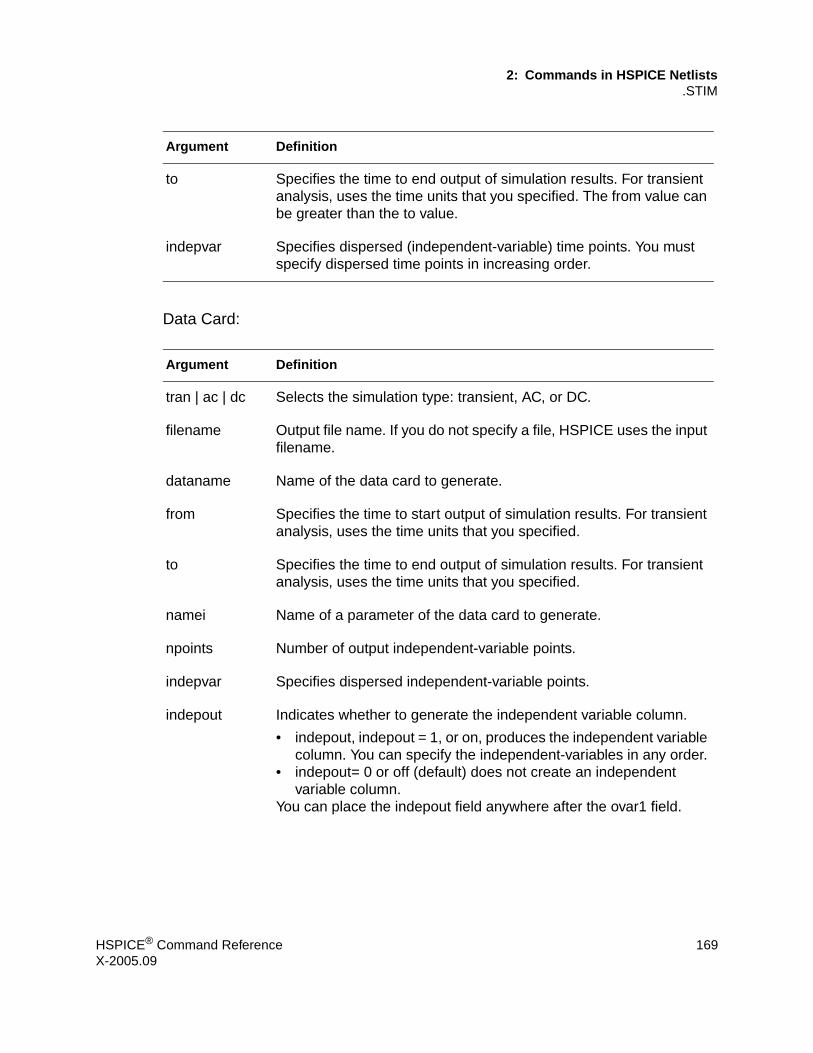
2: Commands in HSPICE Netlists.STIM
Data Card:
to Specifies the time to end output of simulation results. For transient analysis, uses the time units that you specified. The from value can be greater than the to value.
indepvar Specifies dispersed (independent-variable) time points. You must specify dispersed time points in increasing order.
Argument Definition
tran | ac | dc Selects the simulation type: transient, AC, or DC.
filename Output file name. If you do not specify a file, HSPICE uses the input filename.
dataname Name of the data card to generate.
from Specifies the time to start output of simulation results. For transient analysis, uses the time units that you specified.
to Specifies the time to end output of simulation results. For transient analysis, uses the time units that you specified.
namei Name of a parameter of the data card to generate.
npoints Number of output independent-variable points.
indepvar Specifies dispersed independent-variable points.
indepout Indicates whether to generate the independent variable column.
• indepout, indepout = 1, or on, produces the independent variable column. You can specify the independent-variables in any order.
• indepout= 0 or off (default) does not create an independent variable column.
You can place the indepout field anywhere after the ovar1 field.
Argument Definition
HSPICE® Command Reference 169X-2005.09

2: Commands in HSPICE Netlists.STIM
Digital Vector File (Transient Analysis Only):
ovari Output variable that you specify. ovar can be:
• Node voltage.• Element current.• Element templates (HSPICE only).• Parameter string. You cannot use character strings as parameter
values in HSPICE RF.For example:v(1), i(r1), v(2,1), par(’v(1)+v(2)’), LX1(m1), LX2(m1)
Argument Definition
namei Signal name that you specify.
filename Output file name. If you do not specify a file, HSPICE uses the input filename.
ovari Output variable that you specify. ovar can only be a node voltage.
from Specifies the time to start output of simulation results. For transient analysis, uses the time units that you specified.
to Time to the end output of simulation results. For transient analysis, uses the specified time units.The from value can be greater than the to value.
npoints Number of output time points.
indepvar Specifies dispersed independent-variable points. You must specify dispersed time points in increasing order.
vth High voltage threshold.
vtl Low voltage threshold.
voh Logic-high voltage for each output signal.
vol Logic-low voltage for each output signal.
Argument Definition
170 HSPICE® Command ReferenceX-2005.09
2: Commands in HSPICE Netlists.STIM
See Also.DOUT.GRAPH.MEASURE.PLOT.PRINT.PROBE
HSPICE® Command Reference 171X-2005.09

2: Commands in HSPICE Netlists.SUBCKT
.SUBCKT
In HSPICE RF, you cannot replicate output commands within subcircuit (subckt) definitions.
Syntax.SUBCKT subnam n1 <n2 n3 …> <parnam = val> .ENDS
.SUBCKT <SubName><PinList>[<SubDefaultsList>]
.ENDS
.SUBCKT subnam n1 <n2 n3 …> <param=str('string')>
.ENDS
Example 1*FILE SUB2.SP TEST OF SUBCIRCUITS.OPTION LIST ACCT
V1 1 0 1.PARAM P5 = 5 P2 = 10.SUBCKT SUB1 1 2 P4 = 4
R1 1 0 P4R2 2 0 P5X1 1 2 SUB2 P6 = 7X2 1 2 SUB2
.ENDS*.MACRO SUB2 1 2 P6 = 11
R1 1 2 P6R2 2 0 P2
.EOMX1 1 2 SUB1 P4 = 6X2 3 4 SUB1 P6 = 15X3 3 4 SUB2
*.MODEL DA D CJA = CAJA CJP = CAJP VRB = -20
IS = 7.62E-18+ PHI = .5 EXA = .5 EXP = .33.PARAM CAJA = 2.535E-16 CAJP = 2.53E-16.END
The preceding example defines two subcircuits: SUB1 and SUB2. These are resistor-divider networks, whose resistance values are parameters (variables). The X1, X2, and X3 statements call these subcircuits. Because the resistor values are different in each call, these three calls produce different subcircuits.
172 HSPICE® Command ReferenceX-2005.09

2: Commands in HSPICE Netlists.SUBCKT
Example 2.SUBCKT Inv a y Strength = 3
Mp1 <MosPinList> pMosMod L = 1.2uW = ’Strength * 2u’Mn1 <MosPinList> nMosMod L = 1.2u W = ’Strength * 1u’
.ENDS
...xInv0 a y0 Inv $ Default devices: p device = 6u,
$ n device = 3uxInv1 a y1 Inv Strength = 5 $ p device = 10u,
n device = 5uxInv2 a y2 Inv Strength = 1 $ p device = 2u,
n device = 1u...
This example implements an inverter that uses a Strength parameter. By default, the inverter can drive three devices. Enter a new value for the Strength parameter in the element line to select larger or smaller inverters for the application.
Example 3* Using string parameters.subckt IBIS vccq vss out in+ IBIS_FILE=str('file.ibs')+ IBIS_MODEL=str('ibis_model')ven en 0 vccB1 vccq vss out in en v0dq0 vccq vss+ file= str(IBIS_FILE) model=str(IBIS_MODEL).ends
This example implements an IBIS model that uses string parameters to specify the IBIS file name and IBIS model name.
DescriptionYou can create a subcircuit description for a commonly-used circuit, and include one or more references to the subcircuit in your netlist.
To define a subcircuit in your netlist, use the .SUBCKT statement.
When you use hierarchical subcircuits, you can pick default values for circuit elements in a .SUBCKT command. You can use this feature in cell definitions to simulate the circuit with typical values.
HSPICE® Command Reference 173X-2005.09

2: Commands in HSPICE Netlists.SUBCKT
Use the .ENDS statement to terminate a .SUBCKT statement.
See Also.ENDS.EOM.MACRO.MODEL.MODEL.OPTION LIST.PARAM
Argument Definition
subnam Specifies a reference name for the subcircuit model call.
n1 … Node numbers for external reference; cannot be the ground node (zero). Any element nodes that are in the subcircuit, but are not in this list, are strictly local with three exceptions:
• Ground node (zero).• Nodes assigned using BULK = node in MOSFET or BJT models.• Nodes assigned using the .GLOBAL statement.
parnam A parameter name set to a value. Use only in the subcircuit. To override this value, assign it in the subcircuit call, or set a value in a .PARAM statement.
SubDefaultsList <SubParam1>=<Expression>[<SubParam2>=<Expression>...]
174 HSPICE® Command ReferenceX-2005.09

2: Commands in HSPICE Netlists.TEMP
.TEMP
Syntax.TEMP t1 <t2 <t3 ...>>
Example 1.TEMP -55.0 25.0 125.0
The .TEMP statement sets the circuit temperatures for the entire circuit simulation. To simulate the circuit by using individual elements or model temperatures, HSPICE or HSPICE RF uses:■ Temperature as set in the .TEMP statement.■ .OPTION TNOM setting (or the TREF model parameter).■ DTEMP element temperature.
Example 2.TEMP 100D1 N1 N2 DMOD DTEMP=30D2 NA NC DMODR1 NP NN 100 TC1=1 DTEMP=-30.MODEL DMOD D IS=1E-15 VJ=0.6 CJA=1.2E-13 + CJP=1.3E-14 TREF=60.0
In this example:■ The .TEMP statement sets the circuit simulation temperature to 100°C. ■ You do not specify .OPTION TNOM so it defaults to 25°C. ■ The temperature of the diode is 30°C above the circuit temperature as set
in the DTEMP parameter.
That is:■ D1temp = 100°C + 30°C = 130°C. ■ HSPICE or HSPICE RF simulates the D2 diode at 100°C. ■ R1 simulates at 70°C.
HSPICE® Command Reference 175X-2005.09

2: Commands in HSPICE Netlists.TEMP
Because the diode model statement specifies TREF at 60°C, HSPICE or HSPICE RF derates the specified model parameters by:■ 70°C (130°C - 60°C) for the D1 diode.■ 40°C (100°C - 60°C) for the D2 diode. ■ 45°C (70°C - TNOM) for the R1 resistor.
DescriptionTo specify the circuit temperature for an HSPICE or HSPICE RF simulation, use the .TEMP statement, or the TEMP parameter in the .DC, .AC, and .TRAN statements. HSPICE compares the circuit simulation temperature against the reference temperature in the .OPTION TNOM control. HSPICE or HSPICE RF uses the difference between the circuit simulation temperature and the TNOM reference temperature to define derating factors for component values.
In HSPICE RF, you can use multiple .TEMP statements to specify multiple temperatures for different portions of the circuit. HSPICE permits only one temperature for the entire circuit. Multiple definitions of the .TEMP statements in a circuit behave as a sweep function.
Note: HSPICE allows multiple .TEMP statements in the netlist, and performs multiple DC, AC or TRAN analyses for each temperature. Do not set the temperature to the same value multiple times.
See Also.AC.DC.TEMP.OPTION TNOM.TRAN
Argument Definition
t1 t2 Temperatures in ×C, at which HSPICE or HSPICE RF simulates the circuit.
176 HSPICE® Command ReferenceX-2005.09

2: Commands in HSPICE Netlists.TF
.TF
Syntax.TF ov srcnam
Example.TF V(5,3) VIN.TF I(VLOAD) VIN
For the first example, HSPICE or HSPICE RF computes the ratio of V(5,3) to VIN. This is the ratio of small-signal input resistance at VIN to the small-signal output resistance (measured across nodes 5 and 3). If you specify more than one .TF statement in a single simulation, HSPICE or HSPICE RF runs only the last .TF statement.
DescriptionThe transfer function statement (.TF) calculates DC small-signal values for transfer functions (ratio of output variable to input source). You do not need to specify .OP.
The .TF statement defines small-signal output and input for DC small-signal analysis. When you use the .TF statement, HSPICE or HSPICE RF computes:■ DC small-signal value of the transfer function (output/input),.■ Input resistance.■ Output resistance.
.
See Also.DC
Argument Definition
ov Small-signal output variable.
srcnam Small-signal input source.
HSPICE® Command Reference 177X-2005.09
2: Commands in HSPICE Netlists.TITLE
.TITLE
Syntax.TITLE <string_of_up_to_72_characters>
or
<string_of_up_to_72_characters>
Example.TITLE my-design_netlist
DescriptionYou set the simulation title in the first line of the input file. HSPICE or HSPICE RF always reads this line, and uses it as the title of the simulation, regardless of the line’s contents. The simulation prints the title verbatim in each section heading of the output listing file.
To set the title, you can place a .TITLE statement on the first line of the netlist. However, HSPICE or HSPICE RF does not require the .TITLE syntax.
In the second form of the syntax, the string is the first line of the input file. The first line of the input file is always the implicit title. If any statement appears as the first line in a file, simulation interprets it as a title, and does not execute it.
An .ALTER statement does not support using the .TITLE statement. To change a title for a .ALTER statement, place the title content in the .ALTER statement itself.
Argument Definition
string Any character string up to 72 characters long.
178 HSPICE® Command ReferenceX-2005.09

2: Commands in HSPICE Netlists.TRAN
.TRAN
Syntax
Single-Point Analysis
.TRAN tincr1 tstop1 <tincr2 tstop2 ...tincrN tstopN> + <START = val> <UIC>
Double-Point Analysis
.TRAN tincr1 tstop1 <tincr2 tstop2 ...tincrN tstopN>+ <START = val> <UIC> + <SWEEP var type np pstart pstop>
.TRAN tincr1 tstop1 <tincr2 tstop2 ...tincrN tstopN> + <START = val> <UIC> + <SWEEP var START="param_expr1" + STOP="param_expr2"+ STEP="param_expr3">
.TRAN tincr1 tstop1 <tincr2 tstop2 ... tincrN tstopN> + <START=val> <UIC> + <SWEEP var start_expr stop_expr step_expr>
In HSPICE RF, you can run a parameter sweep around a single analysis, but the parameter sweep cannot change any .OPTION value.
Data-Driven Sweep
.TRAN DATA = datanm (HSPICE only; HSPICE RF does not support the .TRAN DATA statement)
.TRAN tincr1 tstop1 <tincr2 tstop2 ...tincrN tstopN> + <START = val> <UIC> <SWEEP DATA = datanm>
.TRAN DATA = datanm<SWEEP var type np pstart pstop>(HSPICE only; HSPICE RF does not support the .TRAN DATA statement)
.TRAN DATA=datanm <SWEEP var START="param_expr1" +STOP="param_expr2" STEP="param_expr3">
.TRAN DATA=datanm + <SWEEP var start_expr stop_expr step_expr>
HSPICE® Command Reference 179X-2005.09

2: Commands in HSPICE Netlists.TRAN
HSPICE RF supports the data-driven syntax only for parameter sweeps:
.tran AB sweepdata=name
Monte Carlo Analysis
.TRAN tincr1 tstop1 <tincr2 tstop2 ...tincrN tstopN>+ <START = val> <UIC> <SWEEP MONTE = list<(>+ <num1:num2> <num3> <num5:num6> <num7> <)> >
Optimization
.TRAN DATA = datanm OPTIMIZE = opt_par_fun+ RESULTS = measnames MODEL = optmod
.TRAN <DATA=filename> SWEEP OPTIMIZE=OPTxxx+ RESULTS=ierr1 ... ierrn MODEL=optmod
Example 1.TRAN 1NS 100NS
This example performs and prints the transient analysis, every 1 ns for 100 ns.
Example 2.TRAN .1NS 25NS 1NS 40NS START = 10NS
This example performs the calculation every 0.1 ns for the first 25 ns; and then every 1 ns, until 40 ns. Printing and plotting begin at 10 ns.
Example 3.TRAN 10NS 1US UIC
This example performs the calculation every 10 ns for 1 µs. This example bypasses the initial DC operating point calculation. It uses the nodal voltages, specified in the .IC statement (or by IC parameters in element statements) to calculate the initial conditions.
Example 4.TRAN 10NS 1US UIC SWEEP TEMP -55 75 10
This example increases the temperature by 10 °C, through the range -55 °C to 75 °C. It also performs transient analysis for each temperature.
Example 5.TRAN 10NS 1US SWEEP load POI 3 1pf 5pf 10pf
180 HSPICE® Command ReferenceX-2005.09
2: Commands in HSPICE Netlists.TRAN
This example analyzes each load parameter value, at 1 pF, 5 pF, and 10 pF.
Example 6.TRAN data = dataname
This example is a data-driven time sweep. It uses a data file as the sweep input. If the parameters in the data statement are controlling sources, then a piecewise linear specification must reference them.
Example 7.TRAN 10NS 1US SWEEP MONTE = 10 firstrun = 11
This example performs the calculation every 10ns for 1us, from the 11th to 20th Monte Carlo trials.
Example 8.TRAN 10NS 1US SWEEP MONTE = list(10 20:30 35:40 50)
This example performs the calculation every 10ns for 1us, at the 10th trial, then from the 20th to the 30th trial, followed by the 35th to the 40th trial, and finally at the 50th Monte Carlo trial.
Description.TRAN starts a transient analysis, which simulates a circuit at a specific time.
Argument Definition
DATA = datanm Data name, referenced in the .TRAN statement (HSPICE only; not supported in HSPICE RF).
MONTE = val Produces a specified number (val) of randomly-generated values. HSPICE uses them to select parameters from a Gaussian, Uniform, or Random Limit distribution (HSPICE only; not supported in HSPICE RF).
np Number of points, or number of points per decade or octave, depending on what keyword precedes it.
param_expr... Expressions you specify: param_expr1...param_exprN.
HSPICE® Command Reference 181X-2005.09
2: Commands in HSPICE Netlists.TRAN
pincr Voltage, current, element, or model parameter; or any temperature increment value. If you set the type variation, use np (number of points), not pincr.
pstart Starting voltage, current, or temperature; or any element or model parameter value. If you set the type variation to POI (list of points), use a list of parameter values, instead of pstart pstop.
pstop Final voltage, current, or temperature; or element or model parameter value.
START Time when printing or plotting begins. The START keyword is optional: you can specify a start time without the keyword.
If you use .TRAN with .MEASURE, a non-zero START time can cause incorrect .MEASURE results. Do not use non-zero START times in .TRAN statements when you also use .MEASURE.
SWEEP Indicates that .TRAN specifies a second sweep.
tincr1… Specifies the printing or plotting increment for printer output, and the suggested computing increment for post-processing.
tstop1… Time when a transient analysis stops incrementing by the first specified time increment (tincr1). If another tincr-tstop pair follows, analysis continues with a new increment.
UIC Uses the nodal voltages specified in the .IC statement (or in the IC = parameters of the various element statements) to calculate initial transient conditions, rather than solving for the quiescent operating point.
type Specifies any of the following keywords:
• DEC – decade variation.• OCT – octave variation (the value of the designated variable is
eight times its previous value).• LIN – linear variation.• POI – list of points.
Argument Definition
182 HSPICE® Command ReferenceX-2005.09
2: Commands in HSPICE Netlists.TRAN
var Name of an independent voltage or current source, any element or model parameter, or the TEMP keyword (indicating a temperature sweep). You can use a source value sweep, referring to the source name (SPICE style). However, if you specify a parameter sweep, a .DATA statement, and a temperature sweep, you must choose a parameter name for the source value, and subsequently refer to it in the .TRAN statement. The parameter name must not start with V or I.
firstrun The val value specifies the number of Monte Carlo iterations to perform. The firstrun value specifies the desired number of iterations. HSPICE runs from num1 to num1+val-1.
list The iterations at which HSPICE performs a Monte Carlo analysis. You can write more than one number after list. The colon represents "from ... to ...". Specifying only one number makes HSPICE run at only the specified point.
Argument Definition
HSPICE® Command Reference 183X-2005.09

2: Commands in HSPICE Netlists.UNPROTECT
.UNPROTECT
Syntax.UNPROTECT
DescriptionIn HSPICE, the .UNPROTECT statement restores normal output functions that a .PROTECT statement restricted. HSPICE RF does not support the .UNPROTECT statement.■ Any elements and models located between .PROTECT and .UNPROTECT
statements, inhibit the element and model listing from the LIST option. ■ Neither the .OPTION NODE cross reference, nor the .OP operating point
printout, list any nodes within the .PROTECT and .UNPROTECT statements.
See Also.PROTECT
184 HSPICE® Command ReferenceX-2005.09

2: Commands in HSPICE Netlists.VEC
.VEC
Syntax.VEC ‘digital_vector_file’
DescriptionYou can call a digital vector file from an HSPICE netlist. A digital vector file consists of three parts:■ Vector Pattern Definition section■ Waveform Characteristics section■ Tabular Data section.
The .VEC file must be a text file. If you transfer it between Unix and Windows, use text mode.
HSPICE® Command Reference 185X-2005.09
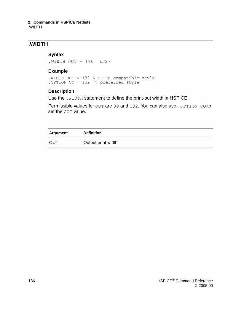
2: Commands in HSPICE Netlists.WIDTH
.WIDTH
Syntax.WIDTH OUT = {80 |132}
Example.WIDTH OUT = 132 $ SPICE compatible style.OPTION CO = 132 $ preferred style
DescriptionUse the .WIDTH statement to define the print-out width in HSPICE.
Permissible values for OUT are 80 and 132. You can also use .OPTION CO to set the OUT value.
Argument Definition
OUT Output print width.
186 HSPICE® Command ReferenceX-2005.09
3: Options in HSPICE Netlists
33Options in HSPICE Netlists
Describes the simulation options you can set using various forms of the .OPTION command.
You can set a wide variety of HSPICE simulation options using the .OPTION command. This chapter provides a list of the various options, arranged by task, followed by detailed descriptions of the individual options.
Options in this chapter fall into the following categories:■ General Control Options■ CPU Options■ Interface Options■ Analysis Options■ Error Options■ Version Option■ Model Analysis Options■ DC Operating Point, DC Sweep, and Pole/Zero Options■ Transient and AC Small Signal Analysis Options■ Transient Control Options■ Input/Output Options
HSPICE® Command Reference 187X-2005.09
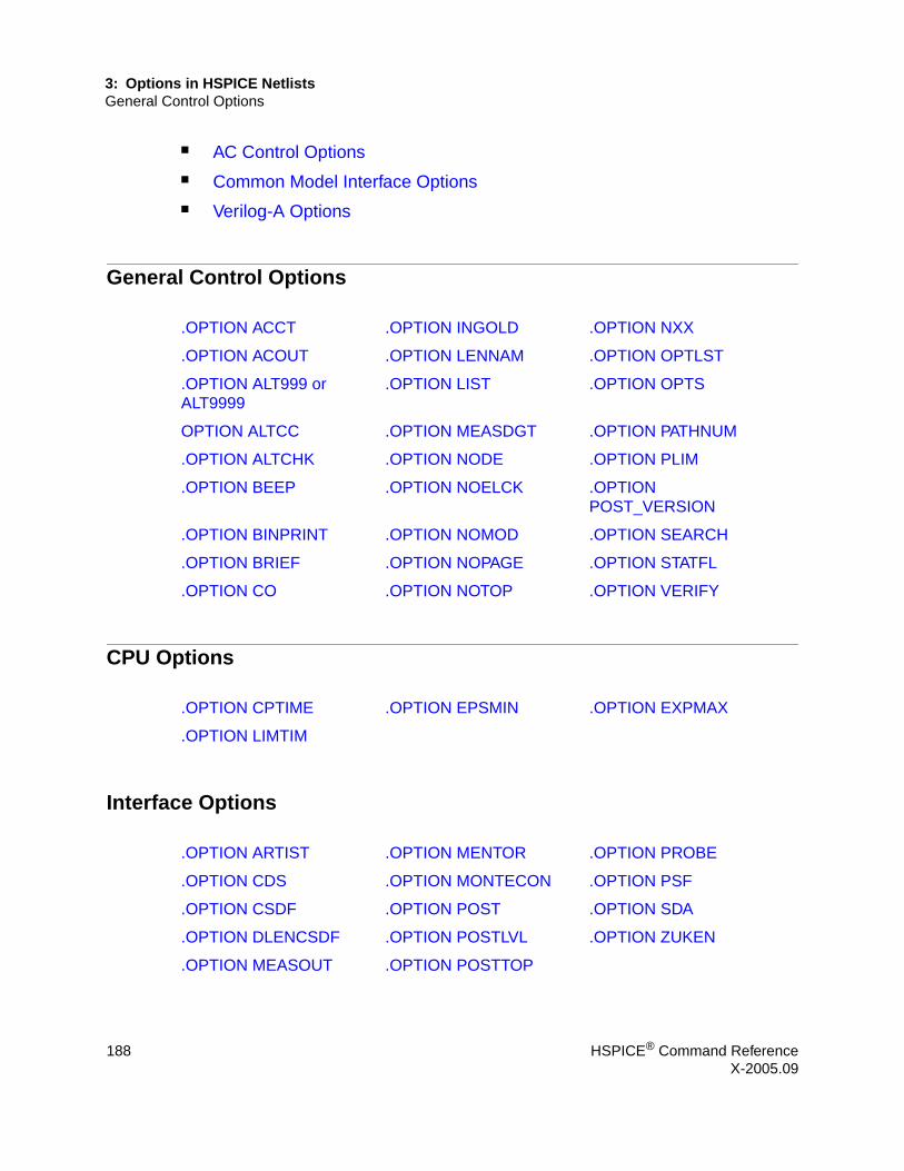
3: Options in HSPICE NetlistsGeneral Control Options
■ AC Control Options■ Common Model Interface Options■ Verilog-A Options
General Control Options
CPU Options
Interface Options
.OPTION ACCT .OPTION INGOLD .OPTION NXX
.OPTION ACOUT .OPTION LENNAM .OPTION OPTLST
.OPTION ALT999 or ALT9999
.OPTION LIST .OPTION OPTS
OPTION ALTCC .OPTION MEASDGT .OPTION PATHNUM
.OPTION ALTCHK .OPTION NODE .OPTION PLIM
.OPTION BEEP .OPTION NOELCK .OPTION POST_VERSION
.OPTION BINPRINT .OPTION NOMOD .OPTION SEARCH
.OPTION BRIEF .OPTION NOPAGE .OPTION STATFL
.OPTION CO .OPTION NOTOP .OPTION VERIFY
.OPTION CPTIME .OPTION EPSMIN .OPTION EXPMAX
.OPTION LIMTIM
.OPTION ARTIST .OPTION MENTOR .OPTION PROBE
.OPTION CDS .OPTION MONTECON .OPTION PSF
.OPTION CSDF .OPTION POST .OPTION SDA
.OPTION DLENCSDF .OPTION POSTLVL .OPTION ZUKEN
.OPTION MEASOUT .OPTION POSTTOP
188 HSPICE® Command ReferenceX-2005.09

3: Options in HSPICE NetlistsAnalysis Options
Analysis Options
Error Options
Version Option
Model Analysis Options
General Model Analysis Options
MOSFET Model Analysis Options
.OPTION ASPEC .OPTION NOISEMINFREQ
.OPTION SEED
.OPTION FFTOUT .OPTION PARHIER .OPTION SPICE
.OPTION LIMPTS
.OPTION BADCHR .OPTION DIAGNOSTIC .OPTION NOWARN
.OPTION WARNLIMIT
.OPTION H9007
.OPTION DCAP .OPTION HIER_SCALE .OPTION TNOM
.OPTION MODSRH .OPTION MODMONTE .OPTION XDTEMP
.OPTION SCALE
.OPTION CVTOL .OPTION DEFNRD .OPTION DEFW
.OPTION DEFAD .OPTION DEFNRS .OPTION SCALM
.OPTION DEFAS .OPTION DEFPD .OPTION WL
.OPTION DEFL .OPTION DEFPS .OPTION WNFLAG
HSPICE® Command Reference 189X-2005.09

3: Options in HSPICE NetlistsDC Operating Point, DC Sweep, and Pole/Zero Options
Inductor Model Analysis Options
BJT and Diode Model Analysis Options
DC Operating Point, DC Sweep, and Pole/Zero Options
DC Accuracy Options
DC Matrix Options
DC Pole/Zero I/O Options
.OPTION GENK .OPTION KLIM
.OPTION EXPLI
.OPTION ABSH .OPTION DI .OPTION RELMOS
.OPTION ABSI .OPTION KCLTEST .OPTION RELV
.OPTION ABSMOS .OPTION MAXAMP .OPTION RELVDC
.OPTION ABSTOL .OPTION RELH
.OPTION ABSVDC .OPTION RELI
.OPTION ITL1 .OPTION PIVOT .OPTION PIVTOL
.OPTION ITL2 .OPTION PIVREF .OPTION SPARSE
.OPTION NOPIV .OPTION PIVREL
.OPTION CAPTAB .OPTION DCCAP .OPTION OPFILE
.OPTION VFLOOR
190 HSPICE® Command ReferenceX-2005.09

3: Options in HSPICE NetlistsTransient and AC Small Signal Analysis Options
DC Convergence Options
DC Initialization Control Options
Transient and AC Small Signal Analysis Options
Transient/AC Accuracy Options
.OPTION CONVERGE .OPTION DV .OPTION ITLPTRAN
.OPTION CSHDC .OPTION GMAX .OPTION NEWTOL
.OPTION DCFOR .OPTION GMINDC .OPTION OFF
.OPTION DCHOLD .OPTION GRAMP .OPTION RESMIN
.OPTION DCSTEP .OPTION GSHDC .OPTION SYMB
.OPTION DCON .OPTION GSHUNT
.OPTION DCTRAN .OPTION ICSWEEP
.OPTION ABSTOL .OPTION GDCPATH .OPTION MAXAMP
.OPTION CAPTAB .OPTION GRAMP .OPTION NEWTOL
.OPTION CSHDC .OPTION GSHDC .OPTION NOPIV
.OPTION DCCAP .OPTION GSHUNT .OPTION OFF
.OPTION DCFOR .OPTION ICSWEEP .OPTION PIVOT
.OPTION DCHOLD .OPTION ITLPTRAN .OPTION PIVREF
.OPTION DCIC .OPTION ITL1 .OPTION PIVTOL
.OPTION DCSTEP .OPTION ITL2 .OPTION RESMIN
.OPTION DV .OPTION KCLTEST .OPTION SPARSE
.OPTION ABSH .OPTION DI .OPTION RELQ
.OPTION ABSV .OPTION GMIN .OPTION RELTOL
.OPTION ACCURATE .OPTION GSHUNT .OPTION RELV
HSPICE® Command Reference 191X-2005.09

3: Options in HSPICE NetlistsTransient and AC Small Signal Analysis Options
Transient/AC Speed Options
Transient/AC Timestep Options
Transient/AC Algorithm Options
.BIASCHK Options
.OPTION ACOUT .OPTION MAXAMP .OPTION RISETIME
.OPTION CHGTOL .OPTION RELH .OPTION TRTOL
.OPTION CSHUNT .OPTION RELI .OPTION VNTOL
.OPTION AUTOSTOP .OPTION BYTOL .OPTION MBYPASS
.OPTION BKPSIZ .OPTION FAST .OPTION SCALE
.OPTION BYPASS .OPTION ITLPZ
.OPTION ABSVAR .OPTION FT .OPTION ITL4
.OPTION DELMAX .OPTION IMAX .OPTION ITL5
.OPTION DVDT .OPTION IMIN .OPTION TIMERES
.OPTION FS .OPTION ITL3
.OPTION DVTR .OPTION ITL5 .OPTION PURETP
.OPTION IMAX .OPTION LVLTIM .OPTION RUNLVL
.OPTION IMIN .OPTION MAXORD .OPTION TRCON
.OPTION ITL3 .OPTION METHOD
.OPTION ITL4 .OPTION MU
.OPTION BIASFILE .OPTION BIAWARN
192 HSPICE® Command ReferenceX-2005.09

3: Options in HSPICE NetlistsTransient Control Options
Transient Control Options
Transient Control Method Options
Transient Control Tolerance Options
Transient Control Limit Options
.OPTION BYPASS .OPTION INTERP .OPTION TRCON
.OPTION CSHUNT .OPTION ITRPRT .OPTION WACC
.OPTION DVDT .OPTION MAXORD
.OPTION GSHUNT .OPTION METHOD
.OPTION ABSH .OPTION FAST .OPTION RELTOL
.OPTION ABSV .OPTION MAXAMP .OPTION RELV
.OPTION ABSVAR .OPTION MBYPASS .OPTION RELVAR
.OPTION ACCURATE .OPTION MU .OPTION SLOPETOL
.OPTION BYTOL .OPTION RELH .OPTION TIMERES
.OPTION CHGTOL .OPTION RELI .OPTION TRTOL
.OPTION DI .OPTION RELQ .OPTION VNTOL
.OPTION AUTOSTOP .OPTION FT .OPTION ITL4
.OPTION BKPSIZ .OPTION GMIN .OPTION ITL5
.OPTION DELMAX .OPTION IMAX .OPTION RMAX
.OPTION DVTR .OPTION IMIN .OPTION RMIN
.OPTION FS .OPTION ITL3 .OPTION VFLOOR
HSPICE® Command Reference 193X-2005.09

3: Options in HSPICE NetlistsInput/Output Options
Transient Control Matrix Options
Iteration Count Dynamic Timestep Options
Input/Output Options
AC Control Options
Common Model Interface Options
Verilog-A Options
.OPTION GMIN .OPTION PIVOT
.OPTION IMAX .OPTION IMIN
.OPTION INTERP .OPTION MEASFILE .OPTION OPTLST
.OPTION ITRPRT .OPTION MEASOUT .OPTION PUTMEAS
.OPTION MEASDGT .OPTION MEASSORT .OPTION UNWRAP
.OPTION MEASFAIL .OPTION MCBRIEF
.OPTION ABSH .OPTION DI .OPTION RELH
.OPTION ACOUT .OPTION MAXAMP .OPTION UNWRAP
.OPTION CMIFLAG .OPTION CUSTCMI
.OPTION SPMODEL .OPTION VAMODEL
194 HSPICE® Command ReferenceX-2005.09

3: Options in HSPICE Netlists.OPTION ABSH
.OPTION ABSH
Syntax.OPTION ABSH=x
DescriptionSets the absolute current change, through voltage-defined branches (voltage sources and inductors). Use this option with options DI and RELH to check for current convergence. The default is 0.0.
See Also.OPTION DI.OPTION RELH
HSPICE® Command Reference 195X-2005.09

3: Options in HSPICE Netlists.OPTION ABSI
.OPTION ABSI
Syntax.OPTION ABSI=x
DescriptionSets the absolute error tolerance for branch currents in diodes, BJTs, and JFETs, during DC and transient analysis. Decrease ABSI, if accuracy is more important than convergence time.
To analyze currents less than 1 nanoamp, change ABSI to a value at least two orders of magnitude smaller than the minimum expected current.
The default is 1e-9 when KCLTEST = 0 or 1e-6 for KCLTEST = 1.
See Also.DC.OPTION KCLTEST.TRAN
196 HSPICE® Command ReferenceX-2005.09

3: Options in HSPICE Netlists.OPTION ABSMOS
.OPTION ABSMOS
Syntax.OPTION ABSMOS=x
DescriptionCurrent error tolerance (for MOSFET devices) in DC or transient analysis. The ABSMOS setting determines whether the drain-to-source current solution has converged. The drain-to-source current converged if:■ The difference between the drain-to-source current in the last iteration,
versus the present iteration, is less than ABSMOS, or ■ This difference is greater than ABSMOS, but the percent change is less than
RELMOS.
If other accuracy tolerances also indicate convergence, HSPICE or HSPICE RF solves the circuit at that timepoint, and calculates the next timepoint solution. For low-power circuits, optimization, and single transistor simulations, set ABSMOS = 1e-12. Default is 1e-6 (amperes).
See Also.DC.OPTION RELMOS.TRAN
HSPICE® Command Reference 197X-2005.09

3: Options in HSPICE Netlists.OPTION ABSTOL
.OPTION ABSTOL
Syntax.OPTION ABSTOL=x
DescriptionSets the absolute error tolerance for branch currents for DC and transient analysis. Decrease ABSTOL, if accuracy is more important than convergence time. ABSTOL is the same as ABSI.
See Also.DC.OPTION ABSI.TRAN
198 HSPICE® Command ReferenceX-2005.09

3: Options in HSPICE Netlists.OPTION ABSV
.OPTION ABSV
Syntax.OPTION ABSV=x
DescriptionSets absolute minimum voltage for DC and transient analysis. ABSV is the same as VNTOL. ■ If accuracy is more critical than convergence, decrease ABSV. ■ If you need voltages less than 50 microvolts, reduce ABSV to two orders of
magnitude less than the smallest desired voltage. This ensures at least two significant digits.
Typically, you do not need to change ABSV, except to simulate a high-voltage circuit. A reasonable value for 1000-volt circuits is 5 to 50 millivolts. The default is 50 (microvolts).
You can use ABSV in HSPICE, but not HSPICE RF.
See Also.DC.OPTION VNTOL.TRAN
HSPICE® Command Reference 199X-2005.09

3: Options in HSPICE Netlists.OPTION ABSVAR
.OPTION ABSVAR
Syntax.OPTION ABSVAR=x
DescriptionSets the absolute limit for the maximum voltage change, from one time point to the next. Use this option with .OPTION DVDT. If the simulator produces a convergent solution that is greater than ABSVAR, then HSPICE discards the solution, sets the timestep to a smaller value, and recalculates the solution. This is called a timestep reversal. The default is 0.5 (volts).
For additional information, see section “DVDT Dynamic Timestep Algorithm” in the HSPICE Simulation and Analysis User Guide.
You can use ABSVAR in HSPICE, but not in HSPICE RF.
See Also.OPTION DVDT
200 HSPICE® Command ReferenceX-2005.09
3: Options in HSPICE Netlists.OPTION ABSVDC
.OPTION ABSVDC
Syntax.OPTION ABSVDC=x
DescriptionSets the minimum voltage for DC and transient analysis. If accuracy is more critical than convergence, decrease ABSVDC. If you need voltages less than 50 micro-volts, reduce ABSVDC to two orders of magnitude less than the smallest voltage. This ensures at least two digits of significance. Typically, you do not need to change ABSVDC, unless you simulate a high-voltage circuit. For 1000-volt circuits, a reasonable value is 5 to 50 millivolts.
The default is the .OPTION VNTOL setting (VNTOL default = 50 mV).
See Also.DC.OPTION VNTOL.TRAN
HSPICE® Command Reference 201X-2005.09

3: Options in HSPICE Netlists.OPTION ACCT
.OPTION ACCT
Syntax.OPTION ACCT
.OPTION ACCT=[1|2]
Example 1.OPTION ACCT=2
The ratio of TOT.ITER to CONV.ITER is the best measure of simulator efficiency. The theoretical ratio is 2:1. In this example the ratio was 2.57:1. SPICE generally has a ratio from 3:1 to 7:1.
In transient analysis, the ratio of CONV.ITER to # POINTS is the measure of the number of points evaluated, to the number of points printed. If this ratio is greater than about 4:1, the convergence and time step control tolerances might be too tight for the simulation.
DescriptionThe ACCT option in HSPICE generates a detailed accounting report.
See Also.DC.TRAN
Argument Definition
.OPTION ACCT Enables reporting.
.OPTION ACCT = 1 (default)
Is the same as ACCT, without arguments.
.OPTION ACCT = 2
Enables reporting, and matrix statistic reporting.
202 HSPICE® Command ReferenceX-2005.09
3: Options in HSPICE Netlists.OPTION ACCURATE
.OPTION ACCURATE
Syntax.OPTION ACCURATE=x
DescriptionSelects a time algorithm that uses LVLTIM = 3 and DVDT = 2 for circuits such as high-gain comparators. Use this option with circuits that combine high gain and large dynamic range to guarantee accurate solutions in HSPICE or HSPICE RF. When set to 1, this option sets these control options:
LVLTIM = 3DVDT = 2RELVAR = 0.2ABSVAR = 0.2FT = 0.2RELMOS = 0.01
The default is 0.
See Also.OPTION ABSVAR.OPTION DVDT.OPTION FT.OPTION LVLTIM.OPTION RELMOS.OPTION RELVAR
HSPICE® Command Reference 203X-2005.09

3: Options in HSPICE Netlists.OPTION ACOUT
.OPTION ACOUT
Syntax.OPTION ACOUT=x
DescriptionAC output calculation method for the difference in values of magnitude, phase, and decibels. Use these values for prints and plots. The default is 1.
The default (ACOUT = 1) selects the HSPICE method, which calculates the difference of the magnitudes of the values. The SPICE method, ACOUT = 0, calculates the magnitude of the differences in HSPICE.
You can use this option in HSPICE, but not in HSPICE RF.
204 HSPICE® Command ReferenceX-2005.09

3: Options in HSPICE Netlists.OPTION ALT999 or ALT9999
.OPTION ALT999 or ALT9999
Syntax.OPTION ALT999
.OPTION ALT9999
DescriptionThis option was developed to allow the.GRAPH statement to create more output files when you ran .ALTER simulations.
This option is obsolete starting with version 2003.09. Without this option, HSPICE can now generate up to 10,000 unique files.
See Also.ALTER.GRAPH
HSPICE® Command Reference 205X-2005.09

3: Options in HSPICE NetlistsOPTION ALTCC
OPTION ALTCC
Syntax.OPTION ALTCC=x
DescriptionEnables HSPICE to only read the input netlist once for multiple .ALTER statements.
ALTCC = 1 enables reading input netlist only once for multiple .ALTER statements.
ALTCC = 0 or -1 disables : HSPICE or HSPICE RF does not output a warning message during transient analysis. HSPICE or HSPICE RF outputs the results, after this transient analysis.
Note: You can use .OPTION ALTCC or .OPTION ALTCC=1 to ignore parsing of an input netlist before an .ALTER statement in the process of standard cell library characterization only when an .ALTER statement changes parameters, source stimulus, analysis, or passive elements. Otherwise, this option is ignored.
See Also.ALTER
206 HSPICE® Command ReferenceX-2005.09

3: Options in HSPICE Netlists.OPTION ALTCHK
.OPTION ALTCHK
Syntax.OPTION ALTCHK=x
DescriptionBy default, HSPICE automatically reports topology errors in the latest elements in your top-level netlist. It also reports errors in elements that you redefine by using the .ALTER statement (altered netlist).
To disable topology checking in redefined elements (that is, to check topology only in the top-level netlist, but not in the altered netlist), set:
.option altchk=0
By default, .OPTION ALTCHK is set to 1:
.option altchk=1
.option altchk
This enables topology checking in elements that you redefine using the .ALTER statement. HSPICE RF does not support .ALTER statements.
See Also.ALTER
HSPICE® Command Reference 207X-2005.09

3: Options in HSPICE Netlists.OPTION ARTIST
.OPTION ARTIST
Syntax.OPTION ARTIST=x
DescriptionARTIST = 2 enables the Cadence Analog Artist interface. This option requires a specific license.
208 HSPICE® Command ReferenceX-2005.09

3: Options in HSPICE Netlists.OPTION ASPEC
.OPTION ASPEC
Syntax.OPTION ASPEC=x
DescriptionSets HSPICE or HSPICE RF to ASPEC-compatibility mode. When you set this option, the simulator reads ASPEC models and netlists, and the results are compatible. The default is 0 (HSPICE mode).
If you set ASPEC, the following model parameters default to ASPEC values:■ ACM = 1: Changes the default values for CJ, IS, NSUB, TOX, U0, and
UTRA.■ Diode Model: TLEV = 1 affects temperature compensation for PB.■ MOSFET Model: TLEV = 1 affects PB, PHB, VTO, and PHI.■ SCALM, SCALE: Sets the model scale factor to microns for length
dimensions.■ WL: Reverses implicit order for stating width and length in a MOSFET
statement. The default (WL=0) assigns the length first, then the width.
See Also.OPTION SCALE.OPTION SCALM.OPTION WL
HSPICE® Command Reference 209X-2005.09

3: Options in HSPICE Netlists.OPTION AUTOSTOP
.OPTION AUTOSTOP
Syntax.OPTION AUTOSTOP
-or-
.OPTION AUTOSTOP=’expression’
Example.option autostop='m1&&m2||m4'.meas tran m1 trig v(bd_a0) val='ddv/2' fall=1 targ v(re_bd) val='ddv/2' rise=1.meas tran m2 trig v(bd_a0) val='ddv/2' fall=2 targ v(re_bd) val='ddv/2' rise=2.meas tran m3 trig v(bd_a0) val='ddv/2' rise=2 targ v(re_bd) val='ddv/2' rise=3.meas tran m4 trig v(bd_a0) val='ddv/2' fall=3 targ v(re_bd) val='ddv/2' rise=4.meas tran m5 trig v(bd_a0) val='ddv/2' rise=3 targ v(re_bd) val='ddv/2' rise=5
In this example, when either m1 and m2 are obtained, or just m4 is obtained, the transient analysis ends.
DescriptionStops a transient analysis in HSPICE or HSPICE RF, after calculating all TRIG-TARG, FIND-WHEN, and FROM-TO measure functions. This option can substantially reduce CPU time. You can use the AUTOSTOP option with any measure type. You can also use the result of the preceding measurement as the next measured parameter.
When using .OPTION AUTOSTOP=’expression’, the ‘expression’ can only involve measure results, a logical AND (&&), or a logical OR(||). Using these types of expressions ends the simulation if any one of a set of .MEASURE statements succeeds, even if the others are not completed.
Also terminates the simulation, after completing all .MEASURE statements. This is of special interest when testing corners.
See Also.MEASURE
210 HSPICE® Command ReferenceX-2005.09

3: Options in HSPICE Netlists.OPTION BADCHR
.OPTION BADCHR
Syntax.OPTION BADCHR
DescriptionGenerates a warning, if it finds a non-printable character in an input file.
HSPICE® Command Reference 211X-2005.09

3: Options in HSPICE Netlists.OPTION BEEP
.OPTION BEEP
Syntax.OPTION BEEP=x
DescriptionBEEP = 1 sounds an audible tone when simulation returns a message, such as:
info: HSPICE job completed.
BEEP = 0 turns off the audible tone.
212 HSPICE® Command ReferenceX-2005.09

3: Options in HSPICE Netlists.OPTION BIASFILE
.OPTION BIASFILE
Syntax.OPTION BIASFILE=x
ExampleOPTION BIASFILE=’biaschk/mos.bias’
DescriptionIf you use this option, HSPICE or HSPICE RF outputs the results of all .BIASCHK commands to a file that you specify. If you do not set this option, HSPICE or HSPICE RF outputs the .BIASCHK results to the *.lis file.
See Also.BIASCHK
HSPICE® Command Reference 213X-2005.09

3: Options in HSPICE Netlists.OPTION BIAWARN
.OPTION BIAWARN
Syntax.OPTION BIAWARN=x
Example.OPTION BIAWARN=1
DescriptionBIAWARN = 1: HSPICE or HSPICE RF immediately outputs a warning message when any local max bias voltage exceeds the limit during transient analysis. After this transient analysis, HSPICE or HSPICE RF outputs the results summary as filtered by noise.
BIAWARN = 0 (default): HSPICE or HSPICE RF does not output a warning message during transient analysis. HSPICE or HSPICE RF outputs the results, after this transient analysis.
See Also.TRAN
214 HSPICE® Command ReferenceX-2005.09

3: Options in HSPICE Netlists.OPTION BINPRINT
.OPTION BINPRINT
Syntax.OPTION BINPRINT
DescriptionOutputs the binning parameters of the CMI MOSFET model. Currently available only for Level 57.
HSPICE® Command Reference 215X-2005.09

3: Options in HSPICE Netlists.OPTION BKPSIZ
.OPTION BKPSIZ
Syntax.OPTION BKPSIZ=x
DescriptionSets the size of the breakpoint table. The default is 5000. This is an old option, provided only for backward-compatibility.
216 HSPICE® Command ReferenceX-2005.09

3: Options in HSPICE Netlists.OPTION BRIEF
.OPTION BRIEF
Syntax.OPTION BRIEF=x
DescriptionStops printback of the data file, until HSPICE or HSPICE RF finds an .OPTION BRIEF = 0 or the .END statement. It also resets the LIST, NODE, and OPTS options, and sets NOMOD. BRIEF = 0 enables printback. The NXX option is the same as BRIEF.
See Also.END.OPTION LIST.OPTION NODE.OPTION NXX.OPTION OPTS
HSPICE® Command Reference 217X-2005.09

3: Options in HSPICE Netlists.OPTION BYPASS
.OPTION BYPASS
Syntax.OPTION BYPASS=x
DescriptionBypasses model evaluations, if the terminal voltages do not change. Can be 0 (off), 1 (on), or 2 (applies to BSIM3v3 and BSIM4 in special cases). To speed-up simulation, this option does not update the status of latent devices. To enable bypassing, set .OPTION BYPASS = 1 for MOSFETs, MESFETs, JFETs, BJTs, or diodes. Default = 1.
Use the BYPASS algorithm cautiously. Some circuit types might not converge, and might lose accuracy in transient analysis and operating-point calculations.
218 HSPICE® Command ReferenceX-2005.09
3: Options in HSPICE Netlists.OPTION BYTOL
.OPTION BYTOL
Syntax.OPTION BYTOL=x
DescriptionSpecifies a voltage tolerance, at which a MOSFET, MESFET, JFET, BJT, or diode becomes latent. HSPICE does not update status of latent devices. The default = MBYPASS x VNTOL.
You can use this option in HSPICE, but not in HSPICE RF.
See Also.OPTION MBYPASS.OPTION VNTOL
HSPICE® Command Reference 219X-2005.09

3: Options in HSPICE Netlists.OPTION CAPTAB
.OPTION CAPTAB
Syntax.OPTION CAPTAB
DescriptionPrints table of single-plate node capacitances for diodes, BJTs, MOSFETs, JFETs, and passive capacitors, at each operating point.
220 HSPICE® Command ReferenceX-2005.09

3: Options in HSPICE Netlists.OPTION CDS
.OPTION CDS
Syntax.OPTION CDS=x
DescriptionCDS = 2 produces a Cadence WSF (ASCII format) post-analysis file for Opus . This option requires a specific license. The CDS option is the same as the SDA option.
See Also.OPTION SDA
HSPICE® Command Reference 221X-2005.09

3: Options in HSPICE Netlists.OPTION CHGTOL
.OPTION CHGTOL
Syntax.OPTION CHGTOL=x
DescriptionSets a charge error tolerance, if you set LVLTIM = 2. Use CHGTOL with RELQ to set the absolute and relative charge tolerance for all HSPICE capacitances. The default is 1e-15 (coulomb).
See Also.OPTION CHGTOL.OPTION LVLTIM.OPTION RELQ
222 HSPICE® Command ReferenceX-2005.09

3: Options in HSPICE Netlists.OPTION CMIFLAG
.OPTION CMIFLAG
Syntax.OPTION CMIFLAG
DescriptionThis option signals to load the dynamically-linked Common Model Interface (CMI) library, libCMImodel.
See Also.OPTION CUSTCMI
HSPICE® Command Reference 223X-2005.09

3: Options in HSPICE Netlists.OPTION CO
.OPTION CO
Syntax.OPTION CO=<column_width>
Example* Narrow print-out (default).OPTION CO=80* Wide print-out.OPTION CO=132
DescriptionThe number of output variables that print on a single line of output, is a function of the number of columns. Use .OPTION CO to set the column width for print-outs in HSPICE.
HSPICE RF does not support the .OPTION CO statement.
You can set up to five output variables per 80-column output, and up to eight output variables per 132-column output withtwelve characters per column. HSPICE automatically creates additional print statements and tables for all output variables beyond the number that the CO option specifies. The default is 80.
See Also.WIDTH
Argument Definition
column_width The number of characters in a single line of output.
224 HSPICE® Command ReferenceX-2005.09

3: Options in HSPICE Netlists.OPTION CONVERGE
.OPTION CONVERGE
Syntax.OPTION CONVERGE=x
DescriptionInvokes different methods to solve non-convergence problems.■ CONVERGE = -1 : Use with DCON = -1 to disable autoconvergence.■ CONVERGE = 0 : Autoconvergence (default).■ CONVERGE = 1 : Uses the Damped Pseudo Transient algorithm. If
simulation does not converge within the set CPU time (in the CPTIME control option), then simulation halts.
■ CONVERGE = 2 : Uses a combination of DCSTEP and GMINDC ramping. Not used in the autoconvergence flow.
■ CONVERGE = 3 : Invokes the source-stepping method. Not used in the autoconvergence flow.
■ CONVERGE = 4 : Uses the gmath ramping method.
Even you did not set it in an .OPTION statement, the CONVERGE option activates if a matrix floating-point overflows, or if HSPICE or HSPICE RF reports a timestep too small error. The default is 0.
If a matrix floating-point overflows, then CONVERGE = 1.
See Also.OPTION DCON.OPTION DCSTEP.OPTION DCTRAN.OPTION GMINDC
HSPICE® Command Reference 225X-2005.09

3: Options in HSPICE Netlists.OPTION CPTIME
.OPTION CPTIME
Syntax.OPTION CPTIME=x
DescriptionSets the maximum CPU time, in seconds, allotted for this simulation job. When the time allowed for the job exceeds CPTIME, HSPICE prints or plots the results up to that point, and concludes the job. Use this option if you are uncertain how long the simulation will take, especially when you debug new data files. Default is 1e7 (400 days).
See Also.OPTION LIMTIM
226 HSPICE® Command ReferenceX-2005.09

3: Options in HSPICE Netlists.OPTION CSDF
.OPTION CSDF
Syntax.OPTION CSDF=x
DescriptionSelects Common Simulation Data Format (Viewlogic-compatible graph data file format).
HSPICE® Command Reference 227X-2005.09

3: Options in HSPICE Netlists.OPTION CSHDC
.OPTION CSHDC
Syntax.OPTION CSHDC=x
DescriptionThe same option as CSHUNT; use only with the CONVERGE option.
You can use the CSHDC option in HSPICE, but not in HSPICE RF.
See Also.OPTION CONVERGE.OPTION CSHUNT
228 HSPICE® Command ReferenceX-2005.09

3: Options in HSPICE Netlists.OPTION CSHUNT
.OPTION CSHUNT
Syntax.OPTION CSHUNT=x
DescriptionCapacitance added from each node to ground in HSPICE or HSPICE RF. Add a small CSHUNT to each node to solve internal timestep too small problems, caused by high-frequency oscillations or numerical noise. The default is 0.
HSPICE® Command Reference 229X-2005.09

3: Options in HSPICE Netlists.OPTION CUSTCMI
.OPTION CUSTCMI
Syntax.OPTION CUSTCMI=x
DescriptionYou set .OPTION CUSTCMI=1 jointly with .OPTION CMIFLAG to turn on gate direct tunneling current modeling and instance parameter support for customer CMI. You set .OPTION CUSTCMI=0 to turn off that feature.
See Also.OPTION CMIFLAG
230 HSPICE® Command ReferenceX-2005.09

3: Options in HSPICE Netlists.OPTION CVTOL
.OPTION CVTOL
Syntax.OPTION CVTOL=x
DescriptionChanges the number of numerical integration steps when calculating the gate capacitor charge for a MOSFET by using CAPOP = 3. See the discussion of CAPOP = 3 in the “Overview of MOSFETS” chapter of the HSPICE Elements and Device Models Manual for explicit equations and discussion.
You can use the .OPTION CVTOL statement in HSPICE, but not in HSPICE RF.
HSPICE® Command Reference 231X-2005.09

3: Options in HSPICE Netlists.OPTION D_IBIS
.OPTION D_IBIS
Syntax.OPTION D_IBIS=’ibis_files_directory’
Example.OPTION d_ibis='/home/user/ibis/models'
DescriptionThe .OPTION D_IBIS option specifies the directory containing the IBIS files. If you specify several directories, then the simulation looks for IBIS files in the local directory (the directory from which you run the simulation). It then checks the directories specified through .OPTION D_IBIS in the order that .OPTION cards appear in the netlist. You can use the D_IBIS option to specify up to four directories.
232 HSPICE® Command ReferenceX-2005.09

3: Options in HSPICE Netlists.OPTION DCAP
.OPTION DCAP
Syntax.OPTION DCAP
DescriptionSelects equations, which HSPICE or HSPICE RF uses to calculate depletion capacitance for Level 1 and 3 diodes, and BJTs. The HSPICE Elements and Device Models Manual describes these equations.
HSPICE® Command Reference 233X-2005.09

3: Options in HSPICE Netlists.OPTION DCCAP
.OPTION DCCAP
Syntax.OPTION DCCAP=x
DescriptionGenerates C-V plots. Prints capacitance values of a circuit (both model and element), during a DC analysis. You can use a DC sweep of the capacitor to generate C-V plots. If not set, MOS device or voltage-variable compacitance values will not be evaluated and the printed value will be zero. The default is 0 (off).
See Also.DC
234 HSPICE® Command ReferenceX-2005.09

3: Options in HSPICE Netlists.OPTION DCFOR
.OPTION DCFOR
Syntax.OPTION DCFOR=x
DescriptionUse with .OPTION DCHOLD and the .NODESET statement to enhance DC convergence.
DCFOR sets the number of iterations to calculate, after a circuit converges in the steady state. The number of iterations after convergence is usually zero so DCFOR adds iterations (and computation time) to the DC circuit solution. DCFOR ensures that a circuit actually, not falsely, converges. The default is 0.
See Also.DC.NODESET.OPTION DCHOLD
HSPICE® Command Reference 235X-2005.09

3: Options in HSPICE Netlists.OPTION DCHOLD
.OPTION DCHOLD
Syntax.OPTION DCHOLD=x
DescriptionUse DCFOR and DCHOLD together to initialize DC analysis. You can use the DCHOLD option in HSPICE, but not in HSPICE RF. DCFOR and DCHOLD enhance the convergence properties of a DC simulation. DCFOR and DCHOLD work with the .NODESET statement. The default is 1.
DCHOLD specifies how many iterations to hold a node, at the .NODESET voltage values. The effects of DCHOLD on convergence differ, according to the DCHOLD value, and the number of iterations before DC convergence.
If a circuit converges in the steady state in fewer than DCHOLD iterations, the DC solution includes the values set in .NODESET.
If a circuit requires more than DCHOLD iterations to converge, HSPICE or HSPICE RF ignores the values set in the .NODESET statement, and calculates the DC solution by using the .NODESET fixed-source voltages open circuited.
See Also.DC.NODESET.OPTION DCFOR
236 HSPICE® Command ReferenceX-2005.09

3: Options in HSPICE Netlists.OPTION DCIC
.OPTION DCIC
Syntax.OPTION DCIC=x
DescriptionIf DCIC=1 (default), each point in a DC sweep analysis acts like an operating point and all .IC commands in the netlist are used.
If DCIC=0, .IC commands in the netlist are ignored for DC sweep analysis.
See Also.IC.DC
HSPICE® Command Reference 237X-2005.09

3: Options in HSPICE Netlists.OPTION DCON
.OPTION DCON
Syntax.OPTION DCON=x
DescriptionIf a circuit cannot converge, HSPICE or HSPICE RF automatically sets DCON = 1, and calculates the following:
, if DV = 1000
Vmax is the maximum voltage, and Imax is the maximum current.
■ If the circuit still cannot converge, HSPICE or HSPICE RF sets DCON = 2, which sets DV = 1e6.
■ If the circuit uses discontinuous models or uninitialized flip-flops, simulation might not converge. Set DCON = -1 and CONVERGE = -1 to disable autoconvergence. HSPICE lists all non-convergent nodes and devices.
See Also.OPTION CONVERGE.OPTION DV
DV max 0.1Vmax
50-----------,
=
GRAMP max 6 log10
Imax
GMINDC------------------------- ,
= ITL1 ITL1 20 GRAMP⋅+=
238 HSPICE® Command ReferenceX-2005.09
3: Options in HSPICE Netlists.OPTION DCSTEP
.OPTION DCSTEP
Syntax.OPTION DCSTEP=x
DescriptionConverts DC model and element capacitors to a conductance to enhance DC convergence properties. HSPICE divides the value of the element capacitors by DCSTEP to model DC conductance. The default is 0 (seconds).
See Also.DC
HSPICE® Command Reference 239X-2005.09

3: Options in HSPICE Netlists.OPTION DCTRAN
.OPTION DCTRAN
Syntax.OPTION DCTRAN=x
DescriptionInvokes different methods to solve non-convergence problems. DCTRAN is an alias for CONVERGE.
See Also.OPTION CONVERGE
240 HSPICE® Command ReferenceX-2005.09

3: Options in HSPICE Netlists.OPTION DEFAD
.OPTION DEFAD
Syntax.OPTION DEFAD=x
DescriptionThe default MOSFET drain diode area in HSPICE. The default is 0.
HSPICE® Command Reference 241X-2005.09

3: Options in HSPICE Netlists.OPTION DEFAS
.OPTION DEFAS
Syntax.OPTION DEFAS=x
DescriptionThe default MOSFET source diode area in HSPICE. The default is 0.
242 HSPICE® Command ReferenceX-2005.09

3: Options in HSPICE Netlists.OPTION DEFL
.OPTION DEFL
Syntax.OPTION DEFL=x
DescriptionThe default MOSFET channel length in HSPICE. The default is 1e-4m.
HSPICE® Command Reference 243X-2005.09

3: Options in HSPICE Netlists.OPTION DEFNRD
.OPTION DEFNRD
Syntax.OPTION DEFNRD=x
DescriptionThe default number of squares for the drain resistor on a MOSFET. The default is 0.
244 HSPICE® Command ReferenceX-2005.09

3: Options in HSPICE Netlists.OPTION DEFNRS
.OPTION DEFNRS
Syntax.OPTION DEFNRS=x
DescriptionThe default number of squares for the source resistor on a MOSFET. The default is 0.
HSPICE® Command Reference 245X-2005.09

3: Options in HSPICE Netlists.OPTION DEFPD
.OPTION DEFPD
Syntax.OPTION DEFPD=x
DescriptionThe default MOSFET drain diode perimeter in HSPICE. The default is 0.
246 HSPICE® Command ReferenceX-2005.09

3: Options in HSPICE Netlists.OPTION DEFPS
.OPTION DEFPS
Syntax.OPTION DEFPS=x
DescriptionThe default MOSFET source diode perimeter in HSPICE. The default is 0.
HSPICE® Command Reference 247X-2005.09

3: Options in HSPICE Netlists.OPTION DEFW
.OPTION DEFW
Syntax.OPTION DEFW=x
DescriptionThe default MOSFET channel width in HSPICE. The default is 1e-4m.
248 HSPICE® Command ReferenceX-2005.09

3: Options in HSPICE Netlists.OPTION DELMAX
.OPTION DELMAX
Syntax.OPTION DELMAX=x
DescriptionSets the maximum Delta of the internal timestep. HSPICE automatically sets the DELMAX value, based on timestep control factors. The initial DELMAX value, shown in the HSPICE output listing, is generally not the value used for simulation.
You can use the DELMAX option in HSPICE, but not in HSPICE RF.
HSPICE® Command Reference 249X-2005.09
3: Options in HSPICE Netlists.OPTION DI
.OPTION DI
Syntax.OPTION DI=x
DescriptionSets the maximum iteration-to-iteration current change, through voltage-defined branches (voltage sources and inductors). Use this option only if the value of the ABSH control option is greater than 0. The default is 0.0.
See Also.OPTION ABSH
250 HSPICE® Command ReferenceX-2005.09

3: Options in HSPICE Netlists.OPTION DIAGNOSTIC
.OPTION DIAGNOSTIC
Syntax.OPTION DIAGNOSTIC
DescriptionLogs the occurrence of negative model conductances.
HSPICE® Command Reference 251X-2005.09

3: Options in HSPICE Netlists.OPTION DLENCSDF
.OPTION DLENCSDF
Syntax.OPTION DLENCSDF=x
DescriptionIf you use the Common Simulation Data Format (Viewlogic graph data file format) as the output format, this digit length option specifies how many digits to include in scientific notation (exponents), or to the right of the decimal point. Valid values are any integer from 1 to 10, and the default is 5.
If you assign a floating decimal point, or if you specify less than 1 or more than 10 digits, HSPICE or HSPICE RF uses the default. For example, it places 5 digits to the right of a decimal point.
252 HSPICE® Command ReferenceX-2005.09
3: Options in HSPICE Netlists.OPTION DV
.OPTION DV
Syntax.OPTION DV=x
DescriptionMaximum iteration-to-iteration voltage change for all circuit nodes in both DC and transient analysis. High-gain bipolar amplifiers can require values of 0.5 to 5.0 to achieve a stable DC operating point. Large CMOS digital circuits frequently require about 1 volt. The default is 1000 (or 1e6 if DCON = 2).
See Also.DC.OPTION DCON.TRAN
HSPICE® Command Reference 253X-2005.09

3: Options in HSPICE Netlists.OPTION DVDT
.OPTION DVDT
Syntax.OPTION DVDT=x
DescriptionAdjusts the timestep, based on rates of change for node voltage. The default is 4.■ 0 - original algorithm■ 1 - fast■ 2 - accurate■ 3,4 - balance speed and accuracy■ You can use the DVDT option in HSPICE, but not in HSPICE RF. ACCURATE
also increases the accuracy of the results.
For additional information, see section “DVDT Dynamic Timestep Algorithm” in the HSPICE Simulation and Analysis User Guide.
See Also.OPTION ACCURATE
254 HSPICE® Command ReferenceX-2005.09

3: Options in HSPICE Netlists.OPTION DVTR
.OPTION DVTR
Syntax.OPTION DVTR=x
DescriptionLimits voltage in transient analysis. The default is 1000.
HSPICE® Command Reference 255X-2005.09

3: Options in HSPICE Netlists.OPTION EPSMIN
.OPTION EPSMIN
Syntax.OPTION EPSMIN=x
DescriptionSpecifies the smallest number that a computer can add or subtract, a constant value. The default is 1e-28.
256 HSPICE® Command ReferenceX-2005.09

3: Options in HSPICE Netlists.OPTION EXPLI
.OPTION EXPLI
Syntax.OPTION EXPLI=x
DescriptionCurrent-explosion model parameter. PN junction characteristics, above the explosion current, are linear. HSPICE or HSPICE RF determines the slope at the explosion point. This improves simulation speed and convergence.
The default is 0.0 amp/AREAeff.
HSPICE® Command Reference 257X-2005.09

3: Options in HSPICE Netlists.OPTION EXPMAX
.OPTION EXPMAX
Syntax.OPTION EXPMAX=x
DescriptionSpecifies the largest exponent that you can use for an exponential, before overflow occurs. Typical value for an IBM platform is 350.
258 HSPICE® Command ReferenceX-2005.09

3: Options in HSPICE Netlists.OPTION FAST
.OPTION FAST
Syntax.OPTION FAST
DescriptionSets additional options, which increase simulation speed withminimal loss of accuracy.
To speed-up simulation, this option does not update the status of latent devices. Use this option for MOSFETs, MESFETs, JFETs, BJTs, and diodes. The default is 0.
You can use FAST in HSPICE, but not HSPICE RF.
A device is latent, if its node voltage variation (from one iteration to the next) is less than the value of either the BYTOL control option, or the BYPASSTOL element parameter. (If FAST is on, HSPICE sets BYTOL to different values for different types of device models.)
Besides the FAST option, you can also use the NOTOP and NOELCK options to reduce input pre-processing time. Increasing the value of the MBYPASS or BYTOL option, also helps simulations to run faster, but can reduce accuracy.
See Also.OPTION BYTOL.OPTION MBYPASS.OPTION NOELCK.OPTION NOTOP
HSPICE® Command Reference 259X-2005.09

3: Options in HSPICE Netlists.OPTION FFTOUT
.OPTION FFTOUT
Syntax.OPTION FFTOUT=x
DescriptionPrints 30 harmonic fundamentals, sorted by size, THD, SNR, and SFDR, but only if you specify a .OPTION FFTOUT statement and a .FFT freq=xxx statement.
You can use the .OPTION FFTOUT statement in HSPICE, but not in HSPICE RF.
See Also.FFT
260 HSPICE® Command ReferenceX-2005.09

3: Options in HSPICE Netlists.OPTION FS
.OPTION FS
Syntax.OPTION FS=x
DescriptionDecreases Delta (internal timestep) by the specified fraction of a timestep (TSTEP) for the first time point of a transient. Decreases the FS value to help circuits that have timestep convergence difficulties. DVDT = 3 uses FS to control the timestep.
■ You specify DELMAX.■ BKPT is related to the breakpoint of the source. ■ The .TRAN statement sets TSTEP. The default is 0.25.
You can use .OPTION FS in HSPICE, but not HSPICE RF.
See Also.OPTION DELMAX.OPTION DVDT.TRAN
Delta FS MIN TSTEP DELMAX BKPT, ,( )[ ]⋅=
HSPICE® Command Reference 261X-2005.09

3: Options in HSPICE Netlists.OPTION FT
.OPTION FT
Syntax.OPTION FT=x
DescriptionDecreases Delta (the internal timestep), by a specified fraction of a timestep (TSTEP) for an iteration set that does not converge. If DVDT = 2 or DVDT = 4, FT controls the timestep. The default is 0.25.
See Also.OPTION DVDT.TRAN
262 HSPICE® Command ReferenceX-2005.09

3: Options in HSPICE Netlists.OPTION GDCPATH
.OPTION GDCPATH
Syntax.OPTION GDCPATH[=x]
DescriptionAdds conductance to nodes having no DC path to ground. You use this option to help solve no DC path to ground problems. If you specify GDCPATH in a netlist without a value, that value is assumed to be 1e-15 (the default). The default is 0 when not specified.
HSPICE® Command Reference 263X-2005.09

3: Options in HSPICE Netlists.OPTION GENK
.OPTION GENK
Syntax.OPTION GENK=x
DescriptionAutomatically computes second-order mutual inductance for several coupled inductors. The default is 1, which enables the calculation.
264 HSPICE® Command ReferenceX-2005.09

3: Options in HSPICE Netlists.OPTION GMAX
.OPTION GMAX
Syntax.OPTION GMAX=x
DescriptionConductance in parallel with a current source for .IC and .NODESET initialization circuitry. Some large bipolar circuits require you to set GMAX = 1 for convergence. The default is 100 (mho).
You can use GMAX in HSPICE, but not in HSPICE RF.
See Also.IC.NODESET
HSPICE® Command Reference 265X-2005.09

3: Options in HSPICE Netlists.OPTION GMIN
.OPTION GMIN
Syntax.OPTION GMIN=x
DescriptionMinimum conductance added to all PN junctions for a time sweep in transient analysis. The default is 1e-12.
266 HSPICE® Command ReferenceX-2005.09

3: Options in HSPICE Netlists.OPTION GMINDC
.OPTION GMINDC
Syntax.OPTION GMINDC=x
DescriptionConductance in parallel to all pn junctions and MOSFET nodes except gate for DC analysis. GMINDC helps overcome DC convergence problems, caused by low values of off-conductance for pn junctions and MOSFETs. You can use GRAMP to reduce GMINDC, by one order of magnitude for each step. Set GMINDC between 1e-4 and the PIVTOL value. The default is 1e-12.
Large values of GMINDC can cause unreasonable circuit response. If your circuit requires large values to converge, suspect a bad model or circuit. If a matrix floating-point overflows, and if GMINDC is 1.0e-12 or less, HSPICE or HSPICE RF sets it to 1.0e-11. HSPICE or HSPICE RF manipulates GMINDC in auto-converge mode.
See Also.DC.OPTION GRAMP.OPTION PIVTOL
HSPICE® Command Reference 267X-2005.09

3: Options in HSPICE Netlists.OPTION GRAMP
.OPTION GRAMP
Syntax.OPTION GRAMP=x
DescriptionHSPICE sets this value during auto-convergence (default is 0). Use GRAMP with the GMINDC option to find the smallest GMINDC value that results in DC convergence.
You can use GRAMP in HSPICE, but not HSPICE RF.
GRAMP specifies a conductance range, over which DC operating point analysis sweeps GMINDC. HSPICE replaces GMINDC values over this range, simulates each value, and uses the lowest GMINDC value where the circuit converges in a steady state.
If you sweep GMINDC between 1e-12 mhos (default) and 1e-6 mhos, GRAMP is 6 (value of the exponent difference, between the default and the maximum conductance limit). In this example:■ HSPICE first sets GMINDC to 1e-6 mhos, and simulates the circuit. ■ If circuit simulation converges, HSPICE sets GMINDC to 1e-7 mhos, and
simulates the circuit.■ The sweep continues until HSPICE simulates all values of the GRAMP ramp.
If the combined GMINDC and GRAMP conductance is greater than 1e-3 mho, false convergence can occur.
See Also.DC.OPTION GMINDC
268 HSPICE® Command ReferenceX-2005.09
3: Options in HSPICE Netlists.OPTION GSHDC
.OPTION GSHDC
Syntax.OPTION GSHDC=x
DescriptionAdds conductance from each node to ground when calculating the DC operating point of the circuit (.OP). The default is 0.
You can use the GSHDC option in HSPICE, but not in HSPICE RF.
See Also.OPTION GSHUNT
HSPICE® Command Reference 269X-2005.09

3: Options in HSPICE Netlists.OPTION GSHUNT
.OPTION GSHUNT
Syntax.OPTION GSHUNT=x
DescriptionAdds conductance from each node to ground. The default is 0. Add a small GSHUNT to each node to help solve Timestep too small problems caused by either high-frequency oscillations or numerical noise.
You can use the GSHUNT option in HSPICE, but not in HSPICE RF.
270 HSPICE® Command ReferenceX-2005.09
3: Options in HSPICE Netlists.OPTION H9007
.OPTION H9007
Syntax.OPTION H9007
DescriptionSets default values for general-control options to correspond to values for HSPICE H9007D. If you set this option, HSPICE does not use the EXPLI model parameter.
See Also.OPTION EXPLI
HSPICE® Command Reference 271X-2005.09
3: Options in HSPICE Netlists.OPTION HIER_SCALE
.OPTION HIER_SCALE
Syntax.OPTION HIER_SCALE=x
DescriptionIf you set the HIER_SCALE option, you can use the S parameter to scale sub-circuits. ■ 0 interprets S as a user-defined parameter. ■ 1 interprets S as a scale parameter.
272 HSPICE® Command ReferenceX-2005.09

3: Options in HSPICE Netlists.OPTION ICSWEEP
.OPTION ICSWEEP
Syntax.OPTION ICSWEEP=x
DescriptionSaves the current analysis result of a parameter or temperature sweep as the starting point in the next analysis in the sweep.■ If ICSWEEP = 1 (default), the next analysis uses the current results. ■ If ICSWEEP = 0, the next analysis does not use the results of the current
analysis.
You can use ICSWEEP in HSPICE, but not in HSPICE RF.
HSPICE® Command Reference 273X-2005.09

3: Options in HSPICE Netlists.OPTION IMAX
.OPTION IMAX
Syntax.OPTION IMAX=x
DescriptionMaximum timestep in timestep algorithms for transient analysis. IMAX sets the maximum iterations to obtain a convergent solution at a timepoint. If the number of iterations needed is greater than IMAX, the internal timestep (Delta) decreases, by a factor equal to the FT transient control option. HSPICE uses the new timestep to calculate a new solution. IMAX also works with the IMIN transient control option. IMAX is the same as ITL4. The default is 8.0.
You can use IMAX in HSPICE, but not HSPICE RF.
See Also.OPTION FT.OPTION IMIN.OPTION ITL4
274 HSPICE® Command ReferenceX-2005.09
3: Options in HSPICE Netlists.OPTION IMIN
.OPTION IMIN
Syntax.OPTION IMIN=x
DescriptionMinimum timestep in timestep algorithms for transient analysis. IMIN is the minimum number of iterations required to obtain convergence. If the number of iterations is less than IMIN, the internal timestep (Delta) doubles.
Use this option to decrease simulation times in circuits where the nodes are stable most of the time (such as digital circuits). If the number of iterations is greater than IMIN, the timestep stays the same, unless the timestep exceeds the IMAX option. IMIN is the same as ITL3. The default is 3.0.
You can use IMIN in HSPICE, but not HSPICE RF.
See Also.OPTION IMAX.OPTION ITL3
HSPICE® Command Reference 275X-2005.09

3: Options in HSPICE Netlists.OPTION INGOLD
.OPTION INGOLD
Syntax.OPTION INGOLD=[0|1|2]
Example.OPTION INGOLD=2
DescriptionBy default, HSPICE or HSPICE RF prints variable values in engineering notation:
F = 1e-15 M = 1e-3P = 1e-12 K = 1e3N = 1e-9 X = 1e6U = 1e-6 G = 1e9
In contrast to exponential form, engineering notation provides two to three extra significant digits, and aligns columns to facilitate comparison. To obtain output in exponential form, specify .OPTION INGOLD = 1 or 2.
See Also
.OPTION MEASDGT
Argument Definition Defaults
INGOLD = 0 (default)
Engineering Format 1.234K123M
INGOLD = 1 G Format (fixed and exponential) 1.234e+03.123
INGOLD = 2 E Format (exponential SPICE) 1.234e+03.123e-1
276 HSPICE® Command ReferenceX-2005.09

3: Options in HSPICE Netlists.OPTION INTERP
.OPTION INTERP
Syntax.OPTION INTERP=x
DescriptionLimits output for post-analysis tools, such as Cadence or Zuken, to only the .TRAN timestep intervals. By default, HSPICE outputs all convergent iterations. INTERP typically produces a much smaller design .tr# file.
Use INTERP = 1 with caution when the netlist includes .MEASURE statements. To compute measure statements, HSPICE uses the post-processing output. Reducing post-processing output can lead to interpolation errors in measure results.
When you run data-driven transient analysis (.TRAN DATA) in an optimization routine, HSPICE forces INTERP=1. HSPICE supports .TRAN DATA; HSPICE RF does not. All measurement results are at the time points specified in the data-driven sweep. To measure only at converged internal timesteps (for example, to calculate the AVG or RMS), set ITRPRT=1.
See Also.MEASURE.OPTION ITRPRT.TRAN
HSPICE® Command Reference 277X-2005.09

3: Options in HSPICE Netlists.OPTION ITL1
.OPTION ITL1
Syntax.OPTION ITL1=x
DescriptionMaximum DC iteration limit. Increasing this value rarely improves convergence in small circuits. Values as high as 400 have resulted in convergence for some large circuits with feedback (such as operational amplifiers and sense amplifiers). However, to converge, most models do not require more than 100 iterations. Set .OPTION ACCT to list how many iterations an operating point requires. The default is 200.
See Also.DC.OPTION ACCT
278 HSPICE® Command ReferenceX-2005.09

3: Options in HSPICE Netlists.OPTION ITL2
.OPTION ITL2
Syntax.OPTION ITL2=x
DescriptionIteration limit for the DC transfer curve. Increasing this limit improves convergence, only for very large circuits. Default is 50.
See Also.DC
HSPICE® Command Reference 279X-2005.09

3: Options in HSPICE Netlists.OPTION ITL3
.OPTION ITL3
Syntax.OPTION ITL3=x
DescriptionMinimum timestep in timestep algorithms for transient analysis. ITL3 is the minimum number of iterations required to obtain convergence. If the number of iterations is less than ITL3, the internal timestep (Delta) doubles.
Use this option to decrease simulation times in circuits where the nodes are stable most of the time (such as digital circuits). If the number of iterations is greater than IMIN, the timestep stays the same, unless the timestep exceeds the IMAX option. ITL3 is the same as IMIN. The default is 3.0.
You can use IMIN in HSPICE, but not HSPICE RF.
See Also.OPTION IMAX.OPTION IMIN
280 HSPICE® Command ReferenceX-2005.09

3: Options in HSPICE Netlists.OPTION ITL4
.OPTION ITL4
Syntax.OPTION ITL4=x
DescriptionMaximum timestep in timestep algorithms for transient analysis. ITL4 sets the maximum iterations to obtain a convergent solution at a timepoint. If the number of iterations needed is greater than ITL4, the internal timestep (Delta) decreases, by a factor equal to the FT transient control option. HSPICE uses the new timestep to calculate a new solution. ITL4 also works with the IMIN transient control option. ITL4 is the same as IMAX. The default is 8.0.
You can use IMAX in HSPICE, but not HSPICE RF.
See Also.OPTION FT.OPTION IMAX.OPTION IMIN
HSPICE® Command Reference 281X-2005.09

3: Options in HSPICE Netlists.OPTION ITL5
.OPTION ITL5
Syntax.OPTION ITL5=x
DescriptionSets an iteration limit for transient analysis. If a circuit uses more than ITL5 iterations, the program prints all results, up to that point. The default is 0.0. allows an infinite number of iterations.
You can use the ITL5 option in HSPICE, but not in HSPICE RF.
282 HSPICE® Command ReferenceX-2005.09

3: Options in HSPICE Netlists.OPTION ITLPTRAN
.OPTION ITLPTRAN
Syntax.OPTION ITLPTRAN=x
DescriptionControls the iteration limit used in the final try of the pseudo-transient method in OP or DC analysis. If simulation fails in the final try of the pseudo-transient method, enlarge this option. The default is 30.
See Also.DC.OP
HSPICE® Command Reference 283X-2005.09

3: Options in HSPICE Netlists.OPTION ITLPZ
.OPTION ITLPZ
Syntax.OPTION ITLPZ=x
DescriptionSets the iteration limit for Pole/Zero analysis. The default is 100.
You can use ITLPZ in HSPICE, but not in HSPICE RF.
284 HSPICE® Command ReferenceX-2005.09
3: Options in HSPICE Netlists.OPTION ITRPRT
.OPTION ITRPRT
Syntax.OPTION ITRPRT
DescriptionPrints output variables at their internal time points. This option might generate a long output list.
HSPICE® Command Reference 285X-2005.09

3: Options in HSPICE Netlists.OPTION KCLTEST
.OPTION KCLTEST
Syntax.OPTION KCLTEST=x
DescriptionActivates KCL (Kirchhoff’s Current Law) test. increases simulation time, especially for large circuits, but very accurately checks the solution. The default is 0.
If you set this value to 1, HSPICE or HSPICE RF sets these options:■ Sets RELMOS and ABSMOS options to 0 (off). ■ Sets ABSI to 1e-6 A.■ Sets RELI to 1e-6.
To satisfy the KCL test, each node must satisfy this condition:
In this equation, the ibs are the node currents.
See Also.OPTION ABSI.OPTION ABSMOS.OPTION RELI.OPTION RELMOS
Σib RELI Σ ib⋅< ABSI+
286 HSPICE® Command ReferenceX-2005.09
3: Options in HSPICE Netlists.OPTION KLIM
.OPTION KLIM
Syntax.OPTION KLIM=x
DescriptionThis option sets the minimum mutual inductance, below which automatic second-order mutual inductance calculation no longer proceeds. KLIM is unitless (analogous to coupling strength, specified in the K Element). Typical KLIM values are between .5 and 0.0. The default is 0.01.
HSPICE® Command Reference 287X-2005.09
3: Options in HSPICE Netlists.OPTION LENNAM
.OPTION LENNAM
Syntax.OPTION LENNAM=x
DescriptionMaximum length of names in the printout of operating point analysis results. Default is 8, and the maximum x value=1024.
288 HSPICE® Command ReferenceX-2005.09

3: Options in HSPICE Netlists.OPTION LIMPTS
.OPTION LIMPTS
Syntax.OPTION LIMPTS=x
DescriptionNumber of points to print or plot in AC analysis. You do not need to set LIMPTS for DC or transient analysis. HSPICE spools the output file to disk. The default is 2001.
See Also.AC.DC.TRAN
HSPICE® Command Reference 289X-2005.09

3: Options in HSPICE Netlists.OPTION LIMTIM
.OPTION LIMTIM
Syntax.OPTION LIMTIM=x
DescriptionAmount of CPU time reserved to generate prints and plots, if a CPU time limit (CPTIME = x) terminates simulation. The default is 2 (seconds), normally sufficient for short printouts and plots.
See Also.OPTION CPTIME
290 HSPICE® Command ReferenceX-2005.09

3: Options in HSPICE Netlists.OPTION LIST
.OPTION LIST
Syntax.OPTION LIST
DescriptionThis option produces an element summary of the input data to print, and calculates effective sizes of elements and the key values. The BRIEF option suppresses the LIST option.
See Also.OPTION BRIEF.OPTION UNWRAP.OPTION VFLOOR
HSPICE® Command Reference 291X-2005.09

3: Options in HSPICE Netlists.OPTION LVLTIM
.OPTION LVLTIM
Syntax.OPTION LVLTIM=x
DescriptionSelects the timestep algorithm for transient analysis. ■ LVLTIM = 1 (default) uses the DVDT timestep control algorithm. ■ LVLTIM = 2 uses the local truncation error (LTE) timestep control method.
You can apply LVLTIM = 2 to the TRAP method. ■ LVLTIM = 3 uses the DVDT timestep control method with timestep reversal.
The local truncation algorithm LVLTIM = 2 (LTE) provides a higher degree of accuracy than LVLTIM = 1 or 3 (DVDT). If you use this option, errors do not propagate from time point to time point, which can result in an unstable solution.
Selecting the GEAR method changes the value of LVLTIM to 2 automatically.
See Also.OPTION CHGTOL.OPTION DVDT.OPTION FS.OPTION FT.OPTION RELQ
292 HSPICE® Command ReferenceX-2005.09
3: Options in HSPICE Netlists.OPTION MAXAMP
.OPTION MAXAMP
Syntax.OPTION MAXAMP=x
DescriptionSets the maximum current, through voltage-defined branches (voltage sources and inductors). If the current exceeds the MAXAMP value, HSPICE or HSPICE RF reports an error. The default is 0.0.
HSPICE® Command Reference 293X-2005.09

3: Options in HSPICE Netlists.OPTION MAXORD
.OPTION MAXORD
Syntax.OPTION MAXORD=x
DescriptionMaximum order of integration for the GEAR method in HSPICE. The x value can be either 1 or 2. ■ MAXORD = 1 uses the backward Euler integration method. ■ MAXORD = 2 (default) is more stable, accurate, and practical.
See Also.OPTION METHOD
294 HSPICE® Command ReferenceX-2005.09

3: Options in HSPICE Netlists.OPTION MBYPASS
.OPTION MBYPASS
Syntax.OPTION MBYPASS=x
DescriptionComputes the default value of the BYTOL control option:
BYTOL = MBYPASSxVNTOL
Also multiplies the RELV voltage tolerance. Set MBYPASS to about 0.1 for precision analog circuits. ■ Default is 1 for DVDT = 0, 1, 2, or 3. ■ Default is 2 for DVDT = 4.
See Also.OPTION BYTOL.OPTION DVDT.OPTION RELV
HSPICE® Command Reference 295X-2005.09

3: Options in HSPICE Netlists.OPTION MCBRIEF
.OPTION MCBRIEF
Syntax.OPTION MCBRIEF=x
DescriptionControls how HSPICE outputs Monte Carlo parameters.■ MCBRIEF=0: Outputs all Monte Carlo parameters (default)■ MCBRIEF=1: Does not output the Monte Carlo parameters■ MCBRIEF=2: Outputs the Monte Carlo parameters into a .lis file only.■ MCBRIEF=3: Outputs the Monte Carlo parameters into the measure files
only.
296 HSPICE® Command ReferenceX-2005.09

3: Options in HSPICE Netlists.OPTION MEASDGT
.OPTION MEASDGT
Syntax.OPTION MEASDGT=x
DescriptionFormats the .MEASURE statement output in both the listing file and the .MEASURE output files (.ma0, .mt0, .ms0, and so on).
The value of x is typically between 1 and 7, although you can set it as high as 10. The default is 4.0.
For example, if MEASDGT = 5, then .MEASURE displays numbers as:■ Five decimal digits for numbers in scientific notation.■ Five digits to the right of the decimal for numbers between 0.1 and 999.
In the listing (.lis), file, all .MEASURE output values are in scientific notation, so .OPTION MEASDGT=5 results in five decimal digits.
Use MEASDGT with .OPTION INGOLD=x to control the output data format.
See Also.OPTION INGOLD.MEASURE
HSPICE® Command Reference 297X-2005.09

3: Options in HSPICE Netlists.OPTION MEASFAIL
.OPTION MEASFAIL
Syntax.OPTION MEASFAIL=0|1
DescriptionYou can assign this option the following values:■ MEASFAIL=0, outputs 0 into the .mt#, .ms#, or .ma# file, and prints failed to
the listing file.■ MEASFAIL=1 (default), prints failed into the .mt#, .ms#, or .ma# file, and
into the listing file.
See Also.MEASURE
298 HSPICE® Command ReferenceX-2005.09

3: Options in HSPICE Netlists.OPTION MEASFILE
.OPTION MEASFILE
Syntax.OPTION MEASFILE=x
DescriptionControls whether measure information outputs to single or multiple files when an .ALTER statement is present in the netlist. You can assign this option the following values:■ MEASFILE=0, outputs measure information to several files.■ MEASFILE=1 (default), outputs measure information to a single file.
See Also.ALTER.MEASURE
HSPICE® Command Reference 299X-2005.09

3: Options in HSPICE Netlists.OPTION MEASSORT
.OPTION MEASSORT
Syntax.OPTION MEASSORT=x
DescriptionIn versions of HSPICE before 2003.09, to automatically sort large numbers of .MEASURE statements, you could use the .OPTION MEASSORT statement.■ .OPTION MEASSORT=0 (default; did not sort .MEASURE statements).■ .OPTION MEASSORT=1 (internally sorted .MEASURE statements).
You needed to set this option to 1 only if you used a large number of .MEASURE statements, where you needed to list similar variables together (to reduce simulation time). For a small number of .MEASURE statements, turning on internal sorting sometimes slowed-down simulation while sorting, compared to not sorting first.
Starting in version 2003.09, this option is obsolete. Now the measure performance is order independent, and HSPICE ignores this option.
See Also.MEASURE
300 HSPICE® Command ReferenceX-2005.09

3: Options in HSPICE Netlists.OPTION MEASOUT
.OPTION MEASOUT
Syntax.OPTION MEASOUT=x
DescriptionThis option outputs .MEASURE statement values and sweep parameters into an ASCII file. Post-analysis processing (AvanWaves or other analysis tools) uses this <design>.mt# file, where # increments for each .TEMP or .ALTER block.
For example, for a parameter sweep of an output load, which measures the delay, the .mt# file contains data for a delay-versus-fanout plot. The default is 1. You can set this option to 0 (off) in the hspice.ini file.
See Also.ALTER.MEASURE.TEMP
HSPICE® Command Reference 301X-2005.09

3: Options in HSPICE Netlists.OPTION MENTOR
.OPTION MENTOR
Syntax.OPTION MENTOR=x
DescriptionMENTOR = 2 enables the Mentor MSPICE-compatible (ASCII) interface. This option requires a specific license.
302 HSPICE® Command ReferenceX-2005.09

3: Options in HSPICE Netlists.OPTION METHOD
.OPTION METHOD
Syntax.OPTION METHOD=GEAR|TRAP
DescriptionSets the numerical integration method for a transient analysis to either GEAR or TRAP. ■ To use GEAR, set METHOD = GEAR, which sets LVLTIM = 2. ■ To change LVLTIM from 2 to 1 or 3, set LVLTIM = 1 or 3, after the
METHOD = GEAR option. This overrides METHOD = GEAR, which sets LVLTIM = 2.
TRAP (trapezoidal) integration usually reduces program execution time with more accurate results. However, this method can introduce an apparent oscillation on printed or plotted nodes, which might not result from circuit behavior. To test this, run a transient analysis by using a small timestep. If oscillation disappears, the cause was the trapezoidal method.
The GEAR method is a filter, removing oscillations that occur in the trapezoidal method. Highly non-linear circuits (such as operational amplifiers) can require very long execution times when you use the GEAR method.
Circuits that do not converge in trapezoidal integration, often converge if you use GEAR. Default is TRAP (trapezoidal).
Gear algorithm:
OPTION METHOD = GEAR
Backward-Euler:
OPTION METHOD = GEAR MU = 0
Trapezoidal algorithm (default):
OPTION METHOD = TRAP
See Also.OPTION LVLTIM.OPTION MU
HSPICE® Command Reference 303X-2005.09

3: Options in HSPICE Netlists.OPTION MODMONTE
.OPTION MODMONTE
Syntax.OPTION MODMONTE=x
DescriptionIf MODMONTE=1, then within a single simulation run, each device that shares the same model card and is in the same Monte Carlo index receives a different random value for parameters that have a Monte Carlo definition.
If MODMONTE=0 (default), then within a single simulation run, each device that shares the same model card and is in the same Monte Carlo index, receives the same random value for its parameters that have a Monte Carlo definition.
304 HSPICE® Command ReferenceX-2005.09
3: Options in HSPICE Netlists.OPTION MODSRH
.OPTION MODSRH
Syntax.OPTION MODSRH=x
Exampleexample.sp:* modsrh used incorrectly.option post modsrh=1xi1 net8 b c t6xi0 a b net8 t6v1 a 0 pulse 3.3 0.0 10E-6 1E-9 1E-9 + 25E-6 50E-6v2 b 0 2v3 c 0 3.model nch nmos level=49 version=3.2.end
This input file automatically searches for t6.inc. If t6.inc includes the nch model, and you set MODSRH to 1, HSPICE or HSPICE RF does not load nch. Do not set MODSRH=1 in this type of file call. Use this option in front of the .MODEL card definition.
DescriptionIf MODSRH=1, HSPICE or HSPICE RF does not load or reference a model described in a .MODEL statement, if the netlist does not use that model. This option shortens simulation run time when the netlist references many models, but no element in the netlist calls those models. The default is MODSRH=0. If MODSRH=1, then the read-in time increases slightly.
See Also.MODEL
HSPICE® Command Reference 305X-2005.09

3: Options in HSPICE Netlists.OPTION MONTECON
.OPTION MONTECON
Syntax.OPTION MONTECON=x
DescriptionContinues a Monte Carlo analysis in HSPICE (not supported in HSPICE RF). Retrieves the next random value, even if non-convergence occurs. A random value can be too large or too small to cause convergence to fail. Other types of analysis can use this Monte Carlo random value.
306 HSPICE® Command ReferenceX-2005.09

3: Options in HSPICE Netlists.OPTION MU
.OPTION MU
Syntax.OPTION MU=x
DescriptionThis option defines the coefficient for trapezoidal integration. The value range is 0.0 to 0.5, and the default is 0.5.
HSPICE® Command Reference 307X-2005.09

3: Options in HSPICE Netlists.OPTION NEWTOL
.OPTION NEWTOL
Syntax.OPTION NEWTOL=x
DescriptionCalculates one or more iterations past convergence for every calculated DC solution and timepoint circuit solution. If you do not set NEWTOL, after HSPICE determines convergence, the convergence routine ends, and the next program step begins. The default is 0.
You can use NEWTOL in HSPICE, but not in HSPICE RF.
308 HSPICE® Command ReferenceX-2005.09

3: Options in HSPICE Netlists.OPTION NODE
.OPTION NODE
Syntax.OPTION NODE=x
Example1 M1:B D2:+ Q4:B
This sample part of a cross reference line indicates that the bulk of M1, the anode of D2, and the base of Q4, all connect to node 1.
DescriptionPrints a node cross reference table. The BRIEF option suppresses NODE. The table lists each node and all elements connected to it. A code indicates the terminal of each element. A colon (:) separates the code from the element name.
The codes are:
+ Diode anode- Diode cathodeB BJT baseB MOSFET or JFET bulkC BJT collectorD MOSFET or JFET drainE BJT emitterG MOSFET or JFET gateS BJT substrateS MOSFET or JFET source
See Also.OPTION BRIEF
HSPICE® Command Reference 309X-2005.09

3: Options in HSPICE Netlists.OPTION NOELCK
.OPTION NOELCK
Syntax.OPTION NOELCK
DescriptionNo element check; bypasses element checking to reduce pre-processing time for very large files.
310 HSPICE® Command ReferenceX-2005.09

3: Options in HSPICE Netlists.OPTION NOISEMINFREQ
.OPTION NOISEMINFREQ
Syntax.OPTION NOISEMINFREQ=x
DescriptionThe .OPTION NOISEMINFREQ command option specifies the minimum frequency of noise analysis. The default is 1e-5. If the frequency of noise analysis is smaller than the minimum frequency, HSPICE automatically sets the frequency for NOISEMINFREQ in noise analysis.
HSPICE® Command Reference 311X-2005.09
3: Options in HSPICE Netlists.OPTION NOMOD
.OPTION NOMOD
Syntax.OPTION NOMOD
DescriptionSuppresses the printout of model parameters.
312 HSPICE® Command ReferenceX-2005.09

3: Options in HSPICE Netlists.OPTION NOPAGE
.OPTION NOPAGE
Syntax.OPTION NOPAGE
DescriptionSuppresses page ejects for title headings.
HSPICE® Command Reference 313X-2005.09

3: Options in HSPICE Netlists.OPTION NOPIV
.OPTION NOPIV
Syntax.OPTION NOPIV=x
DescriptionPrevents HSPICE or HSPICE RF from automatically switching to pivoting matrix factors, if a nodal conductance is less than PIVTOL. NOPIV inhibits pivoting.
See Also.OPTION PIVTOL
314 HSPICE® Command ReferenceX-2005.09

3: Options in HSPICE Netlists.OPTION NOTOP
.OPTION NOTOP
Syntax.OPTION NOTOP
DescriptionSuppresses topology checks to increase the speed for pre-processing very large files.
HSPICE® Command Reference 315X-2005.09

3: Options in HSPICE Netlists.OPTION NOWARN
.OPTION NOWARN
Syntax.OPTION NOWARN
DescriptionSuppresses all warning messages, except those generated from statements in .ALTER blocks.
See Also.ALTER
316 HSPICE® Command ReferenceX-2005.09

3: Options in HSPICE Netlists.OPTION NUMDGT
.OPTION NUMDGT
Syntax.OPTION NUMDGT=x
DescriptionThis option controls the listing printout (.lis) accuracy. The value of x is typically between 1 and 7, although you can set it as high as 10. The default is 4.0. This option does not affect the accuracy of the simulation.
This option does affect the results files (ASCII and binary) if you use the .OPTION POST_VERSION = 2001 setting. The default setting of results files for printout accuracy is 5 digits.
See Also.OPTION POST_VERSION
HSPICE® Command Reference 317X-2005.09
3: Options in HSPICE Netlists.OPTION NXX
.OPTION NXX
Syntax.OPTION NXX
DescriptionStops printback of the data file, until HSPICE or HSPICE RF finds an .OPTION BRIEF=0 or the .END statement. It also resets the LIST, NODE and OPTS options, and sets NOMOD. When BRIEF=0, it enables printback. NXX is the same as BRIEF.
See Also.OPTION BRIEF.OPTION LIST.OPTION NODE.OPTION OPTS
318 HSPICE® Command ReferenceX-2005.09

3: Options in HSPICE Netlists.OPTION OFF
.OPTION OFF
Syntax.OPTION OFF=x
DescriptionFor all active devices, initializes terminal voltages to zero, if you did not initialize them to other values. For example, if you did not initialize both drain and source nodes of a transistor (using .NODESET, .IC statements, or connecting them to sources), then OFF initializes all nodes of the transistor to 0.
HSPICE or HSPICE RF checks the OFF option, before element IC parameters. If you assigned an element IC parameter to a node, simulation initializes the node to the element IC parameter value, even if the OFF option previously set it to 0.
You can use the OFF element parameter to initialize terminal voltages to 0 for specific active devices. Use the OFF option to help find exact DC operating-point solutions for large circuits.
See Also.DC.IC.NODESET
HSPICE® Command Reference 319X-2005.09

3: Options in HSPICE Netlists.OPTION OPFILE
.OPTION OPFILE
Syntax.OPTION OPFILE=value
DescriptionThe OPFILE option outputs the operating point information to a file. value can be 0 or 1. ■ If value is 1, operating point information is output to a file named
<design>.dp#. ■ If value is 0, the operating point information outputs to stdout.
320 HSPICE® Command ReferenceX-2005.09

3: Options in HSPICE Netlists.OPTION OPTLST
.OPTION OPTLST
Syntax.OPTION OPTLIST=x
DescriptionOutputs additional optimization information:■ OPTLIST=0: No information (default).■ OPTLIST=1: Prints parameter, Broyden update, and bisection results
information.■ OPTLIST=2: Prints gradient, error, Hessian, and iteration information.■ OPTLIST=3: Prints all of the above and Jacobian.
HSPICE® Command Reference 321X-2005.09
3: Options in HSPICE Netlists.OPTION OPTS
.OPTION OPTS
Syntax.OPTION OPTS
DescriptionPrints the current settings for all control options. If you change any of the default values of the options, the OPTS option prints the values that the simulation actually uses. The BRIEF option suppresses OPTS.
See Also.OPTION BRIEF
322 HSPICE® Command ReferenceX-2005.09

3: Options in HSPICE Netlists.OPTION PARHIER
.OPTION PARHIER
Syntax.OPTION PARHIER = < GLOBAL | LOCAL >
Example.OPTION parhier=<global | local>.PARAM DefPwid = 1u.SUBCKT Inv a y DefPwid = 2u DefNwid = 1u
Mp1 <MosPinList> pMosMod L = 1.2u W = DefPwidMn1 <MosPinList> nMosMod L = 1.2u W = DefNwid
.ENDS
This example explicitly shows the difference between local and global scoping for using parameters in sub-circuits.
DescriptionUse the .OPTION OPTLST parameter to specify scoping rules.
The default setting is GLOBAL.
See Also.OPTION OPTLST
HSPICE® Command Reference 323X-2005.09

3: Options in HSPICE Netlists.OPTION PATHNUM
.OPTION PATHNUM
Syntax.OPTION PATHNUM
DescriptionPrints subcircuit path numbers, instead of path names.
324 HSPICE® Command ReferenceX-2005.09

3: Options in HSPICE Netlists.OPTION PIVOT
.OPTION PIVOT
Syntax.OPTION PIVOT=x
DescriptionSelects a pivot algorithms. Use these algorithms to reduce simulation time, and to achieve convergence in circuits that produce hard-to-solve matrix equations. To select the pivot algorithm, set PIVOT as follows:■ PIVOT=0: Original non-pivoting algorithm.■ PIVOT=1: Original pivoting algorithm.■ PIVOT=2: Picks the largest pivot in the row.■ PIVOT=3: Picks the best pivot in a row.■ PIVOT=10 (default): Fast, non-pivoting algorithm; requires more memory.■ PIVOT=11: Fast, pivoting algorithm; requires more memory than PIVOT
values less than 11.■ PIVOT=12: Picks the largest pivot in the row; requires more memory than
PIVOT values less than 12.■ PIVOT=13: Fast, best pivot: faster; requires more memory than PIVOT
values less than 13.
The fastest algorithm is PIVOT = 13, which can improve simulation time up to ten times, on very large circuits. However, PIVOT = 13 requires substantially more memory for simulation.
Some circuits with large conductance ratios, such as switching regulator circuits, might require pivoting.
If PIVTOL = 0, HSPICE or HSPICE RF automatically changes from non-pivoting to a row-pivot strategy, if it detects any diagonal-matrix entry less than PIVTOL. This strategy provides the time and memory advantages of non-pivoting inversion, and avoids unstable simulations and incorrect results. Use .OPTION NOPIV to prevent HSPICE or HSPICE RF from pivoting. For very large circuits, PIVOT = 10, 11, 12, or 13, can require excessive memory.
If HSPICE or HSPICE RF switches to pivoting during a simulation, it displays the message followed by the node numbers that cause the problem:
pivot change on the fly
HSPICE® Command Reference 325X-2005.09
3: Options in HSPICE Netlists.OPTION PIVOT
Use .OPTION NODE to cross-reference a node to an element. The SPARSE option is the same as PIVOT.
See Also.OPTION NODE.OPTION NOPIV.OPTION PIVREF.OPTION PIVREL.OPTION PIVTOL.OPTION SPARSE
326 HSPICE® Command ReferenceX-2005.09

3: Options in HSPICE Netlists.OPTION PIVREF
.OPTION PIVREF
Syntax.OPTION PIVREF=x
DescriptionPivot reference. Use PIVREF in PIVOT = 11, 12, or 13 to limit the size of the matrix. The default is 1e+8.
See Also.OPTION PIVOT
HSPICE® Command Reference 327X-2005.09

3: Options in HSPICE Netlists.OPTION PIVREL
.OPTION PIVREL
Syntax.OPTION PIVREL=x
DescriptionSets the maximum and minimum ratio of a row or matrix. Use only if PIVOT = 1. Large values for PIVREL can result in very long matrix pivot times. If the value is too small, however, no pivoting occurs. Start with small values of PIVREL by using an adequate (but not excessive) value for convergence and accuracy. The default is 1E-20 (max = 1e-20, min = 1).
See Also.OPTION PIVOT
328 HSPICE® Command ReferenceX-2005.09

3: Options in HSPICE Netlists.OPTION PIVTOL
.OPTION PIVTOL
Syntax.OPTION PIVTOL=x
DescriptionAbsolute minimum value for which HSPICE or HSPICE RF accepts a matrix entry as a pivot. If PIVOT=0, PIVTOL is the minimum conductance in the matrix. The default is 1.0e-15.
PIVTOL must be less than GMIN or GMINDC. Values that approach 1 increase the pivot.
See Also.OPTION GMIN.OPTION GMINDC.OPTION PIVOT
HSPICE® Command Reference 329X-2005.09

3: Options in HSPICE Netlists.OPTION PLIM
.OPTION PLIM
Syntax.OPTION PLIM
DescriptionSpecifies plot size limits for current and voltage plots:■ Finds a common plot limit, and plots all variables on one graph, at the same
scale■ Enables SPICE-type plots in HSPICE, which create a separate scale and
axis for each plot variable
You can use SPICE-compatibility mode in HSPICE, but not in HSPICE RF.
This option does not affect postprocessing of graph data.
330 HSPICE® Command ReferenceX-2005.09

3: Options in HSPICE Netlists.OPTION POST
.OPTION POST
Syntax.OPTION POST=[0|1|2|3|ASCII|BINARY]
Example.OPTION POST=2
DescriptionUse an .OPTION POST statement to display high-resolution AvanWaves plots of simulation results, on either a graphics terminal or a high-resolution laser printer. Use .OPTION POST to provide output, without specifying other parameters. POST has defaults, which supply usable data to most parameters.■ POST = 0: Does not output simulation results.■ POST = 1, BINARY: (Default) Output format is binary.■ POST = 2, ASCII: Output format is ASCII.■ POST = 3: Output format is New Wave binary.
See Also.OPTION POST_VERSION
HSPICE® Command Reference 331X-2005.09

3: Options in HSPICE Netlists.OPTION POSTLVL
.OPTION POSTLVL
Syntax.OPTION POSTLVL=x
Example.OPTION POSTLVL=2
This example limits the data written to the waveform file to only the second-level nodes.
DescriptionThe .OPTION POSTLVL option limits the data to only the x level nodes, which is written to your waveform file.
332 HSPICE® Command ReferenceX-2005.09

3: Options in HSPICE Netlists.OPTION POST_VERSION
.OPTION POST_VERSION
Syntax.OPTION POST_VERSION=x
DescriptionSets the post-processing output version:■ x = 9007 truncates the node name in the post-processor output file to a
maximum of 16 characters. ■ x = 9601 (default) sets the node name length for the output file consistent
with the input restrictions (1024 characters), and limits the number of output variables to 9999.
■ x = 2001 shows the new output file header, which includes the right number of output variables rather than **** when the number exceeds 9999. This option also changes the number of digits precision in results files to match the value of .OPTION NUMDGT (when < 5).
If you set .OPTION POST_VERSION = 2001 POST= 2 in the netlist, then HSPICE or HSPICE RF returns more-accurate ASCII results.
.option post_version=2001
To use binary values (with double precision) in the output file, include the following in the input file:
*******************************************.option post (or post=1) post_version=2001*******************************************
For more accurate simulation results, comment this format.
See Also.OPTION NUMDGT.OPTION POST
HSPICE® Command Reference 333X-2005.09

3: Options in HSPICE Netlists.OPTION POSTTOP
.OPTION POSTTOP
Syntax.OPTION POSTTOP=n
ExamplePOSTTOP = 1
This example limits the data written to the waveform file to only the top-level nodes.
DescriptionThe .OPTION POSTTOP option limits the data to only the data from the top n level nodes, which is written to your waveform file. If you do not specify either the .OPTION PROBE or the .OPTION POSTTOP options, then HSPICE outputs all levels.
To enable the waveform display interface, you also need the .OPTION POST option.
See Also.OPTION POST.OPTION PROBE
334 HSPICE® Command ReferenceX-2005.09

3: Options in HSPICE Netlists.OPTION PROBE
.OPTION PROBE
Syntax.OPTION PROBE=x
DescriptionLimits post-analysis output to only variables specified in .PROBE, .PRINT, .PLOT, and .GRAPH statements. HSPICE RF supports .PROBE and .PRINT statements, but does not support .PLOT and .GRAPH statements. By default, HSPICE or HSPICE RF outputs all voltages and power supply currents in addition to variables listed in .PROBE, .PRINT, .PLOT, and .GRAPH statements. PROBE significantly decreases the size of simulation output files.
See Also.GRAPH.PLOT.PRINT.PROBE
HSPICE® Command Reference 335X-2005.09

3: Options in HSPICE Netlists.OPTION PSF
.OPTION PSF
Syntax.OPTION PSF=x
DescriptionSpecifies whether HSPICE or HSPICE RF outputs binary or ASCII data when you run an HSPICE simulation from Cadence Analog Artist.
The value of x can be 1 or 2. ■ If x is 2, HSPICE or HSPICE RF produces ASCII output. ■ If .OPTION ARTIST PSF = 1, HSPICE produces binary output.
See Also.OPTION ARTIST
336 HSPICE® Command ReferenceX-2005.09

3: Options in HSPICE Netlists.OPTION PURETP
.OPTION PURETP
Syntax.OPTION PURETP=x
DescriptionIntegration method to use for reversal time point. The default is 0. If you set PURETP=1, then if HSPICE finds non-convergence, it uses TRAP (instead of B.E) for the reversed time point. Use this option with the method=TRAP statement to help some oscillating circuits to oscillate, if the default simulation process cannot satisfy the result.
HSPICE® Command Reference 337X-2005.09

3: Options in HSPICE Netlists.OPTION PUTMEAS
.OPTION PUTMEAS
Syntax.OPTION PUTMEAS=0|1
DescriptionThe .OPTION PUTMEAS option controls the output variables, listed in the .MEASURE statement.■ 0: Does not save variable values, which are listed in the .MEASURE
statement, into the corresponding output file (such as .tr#, .ac# or .sw#). This option decreases the size of the output file.
■ 1: Default. Saves variable values, which are listed in the .MEASURE statement, into the corresponding output file (such as .tr#, .ac# or .sw#). This option is similar to the output of HSPICE 2000.4.
See Also.MEASURE
338 HSPICE® Command ReferenceX-2005.09

3: Options in HSPICE Netlists.OPTION RELH
.OPTION RELH
Syntax.OPTION RELH=x
DescriptionRelative current tolerance, through voltage-defined branches (voltage sources and inductors). Use RELH to check current convergence, but only if the value of the ABSH control option is greater than zero. The default is 0.05.
You can use RELH in HSPICE, but not in HSPICE RF.
See Also.OPTION ABSH
HSPICE® Command Reference 339X-2005.09

3: Options in HSPICE Netlists.OPTION RELI
.OPTION RELI
Syntax.OPTION RELI=x
DescriptionSets the relative error/tolerance change, from iteration to iteration. This parameter determines convergence for all currents in diode, BJT, and JFET devices. (RELMOS sets tolerance for MOSFETs). This is the change in current, from the value calculated at the previous timepoint. ■ Default = 0.01 for .OPTION KCLTEST = 0.■ Default = 1e-6 for .OPTION KCLTEST = 1.
See Also.OPTION RELMOS.OPTION KCLTEST
340 HSPICE® Command ReferenceX-2005.09

3: Options in HSPICE Netlists.OPTION RELMOS
.OPTION RELMOS
Syntax.OPTION RELMOS=x
DescriptionSets the relative error tolerance (percent) for drain-to-source current, from iteration-to-iteration. This parameter determines convergence for currents in MOSFET devices. (.OPTION RELI sets the tolerance for other active devices.) Sets the change in current, from the value calculated at the previous timepoint. HSPICE or HSPICE RF uses the .OPTION RELMOS value, only if the current is greater than the .OPTION ABSMOS floor value. The default is 0.05.
See Also.OPTION ABSMOS.OPTION RELI.OPTION RELMOS
HSPICE® Command Reference 341X-2005.09

3: Options in HSPICE Netlists.OPTION RELQ
.OPTION RELQ
Syntax.OPTION RELQ=x
DescriptionUsed in the timestep algorithm for local truncation error (LVLTIM = 2). RELQ changes the timestep size. If the capacitor charge calculation (in the present iteration) exceeds that of the past iteration by a percentage greater than the RELQ value, then HSPICE reduces the internal timestep (Delta). The default is 0.01.
You can use RELQ in HSPICE, but not in HSPICE RF.
See Also.OPTION LVLTIM
342 HSPICE® Command ReferenceX-2005.09
3: Options in HSPICE Netlists.OPTION RELTOL
.OPTION RELTOL
Syntax.OPTION RELTOL=x
DescriptionRelative error tolerance for voltages. Use RELTOL with the ABSV control option to determine voltage convergence. Increasing RELTOL increases the relative error. RELTOL is the same as RELV. RELI and RELVDC options default to the RELTOL value. The default is 1e-3.
You can use the RELTOL and RELV options in HSPICE, but not in HSPICE RF.
See Also.OPTION ABSV.OPTION RELI.OPTION RELV.OPTION RELVDC
HSPICE® Command Reference 343X-2005.09

3: Options in HSPICE Netlists.OPTION RELV
.OPTION RELV
Syntax.OPTION RELV=x
DescriptionSets the relative error tolerance for voltages. If voltage or current exceeds the absolute tolerances, a RELV test determines convergence. Increasing RELV increases the relative error. You should generally maintain RELV at its default value. RELV conserves simulator charge. For voltages, RELV is the same as RELTOL. The default is 1e-3.
See Also.OPTION RELTOL
344 HSPICE® Command ReferenceX-2005.09

3: Options in HSPICE Netlists.OPTION RELVAR
.OPTION RELVAR
Syntax.OPTION RELVAR=x
DescriptionUse this option with ABSVAR, and the DVDT timestep algorithm. RELVAR sets the relative voltage change for LVLTIM = 1 or 3. If the node voltage at the current time point exceeds the node voltage at the previous time point by RELVAR, then HSPICE reduces the timestep, and calculates a new solution at a new time point. The default is 0.30 (30%).
For additional information, see section “DVDT Dynamic Timestep Algorithm” in the HSPICE Simulation and Analysis User Guide.
You can use the RELVAR option in HSPICE, but not in HSPICE RF.
See Also.OPTION ABSVAR.OPTION DVDT.OPTION LVLTIM
HSPICE® Command Reference 345X-2005.09

3: Options in HSPICE Netlists.OPTION RELVDC
.OPTION RELVDC
Syntax.OPTION RELVDC=x
DescriptionSets the relative error tolerance for voltages. If voltages or currents exceed their absolute tolerances, the RELVDC test determines convergence. Increasing RELVDC increases the relative error. You should generally maintain RELVDC at its default value. RELVDC conserves simulator charge. Default is RELTOL (RELTOL default = 1e-3).
See Also.OPTION RELTOL
346 HSPICE® Command ReferenceX-2005.09

3: Options in HSPICE Netlists.OPTION RESMIN
.OPTION RESMIN
Syntax.OPTION RESMIN=x
DescriptionMinimum resistance for all resistors, including parasitic and inductive resistances. The default is 1e-5 (ohm), and the range is 1e-15 to 10 ohm.
HSPICE® Command Reference 347X-2005.09
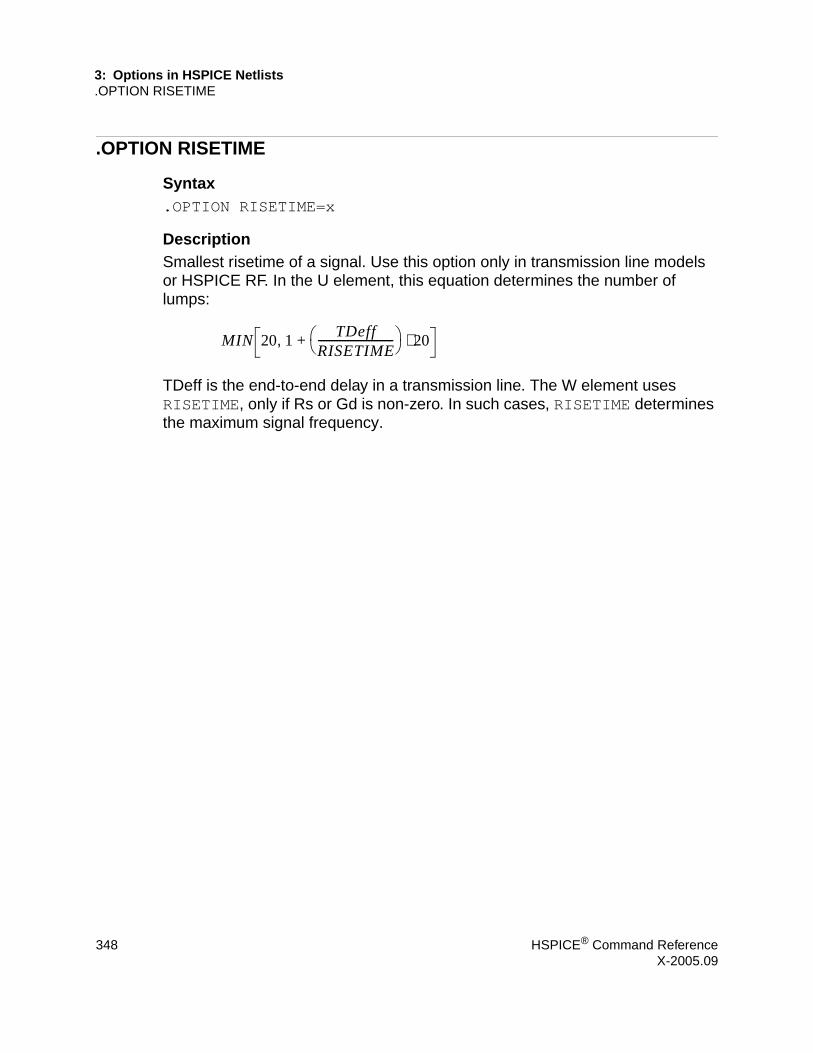
3: Options in HSPICE Netlists.OPTION RISETIME
.OPTION RISETIME
Syntax.OPTION RISETIME=x
DescriptionSmallest risetime of a signal. Use this option only in transmission line models or HSPICE RF. In the U element, this equation determines the number of lumps:
TDeff is the end-to-end delay in a transmission line. The W element uses RISETIME, only if Rs or Gd is non-zero. In such cases, RISETIME determines the maximum signal frequency.
MIN 20 1TDeff
RISETIME---------------------------- 20⋅+,
348 HSPICE® Command ReferenceX-2005.09

3: Options in HSPICE Netlists.OPTION RMAX
.OPTION RMAX
Syntax.OPTION RMAX=x
DescriptionSets the TSTEP multiplier, which controls the maximum value (DELMAX) for the Delta of the internal timestep:
DELMAX = TSTEP x RMAX
■ The default is 5, if DVDT is 4 and LVLTIM is 1.■ Otherwise, the default is 2.
The maximum value is 1e+9, the minimum value is 1e-9. The recommended maximum value is 1e+5. Supported in HSPICE and HSPICE RF.
For a discussion about timestep control, see section “Timestep Control for Accuracy” in the HSPICE Simulation and Analysis User Guide.
See Also.OPTION DELMAX.OPTION DVDT.OPTION LVLTIM
HSPICE® Command Reference 349X-2005.09

3: Options in HSPICE Netlists.OPTION RMIN
.OPTION RMIN
Syntax.OPTION RMIN=x
DescriptionSets the minimum value of Delta (internal timestep). An internal timestep smaller than RMIN x TSTEP, terminates the transient analysis, and reports an internal timestep too small error. If the circuit does not converge in IMAX iterations, Delta decreases by the amount you set in the FT option. The default is 1.0e-9.
You can use RMIN in HSPICE, but not HSPICE RF.
See Also.OPTION FT.OPTION IMAX
350 HSPICE® Command ReferenceX-2005.09

3: Options in HSPICE Netlists.OPTION RUNLVL
.OPTION RUNLVL
Syntax.OPTION RUNLVL=x
DescriptionThe value for the .OPTION RUNLVL option controls the speed and accuracy trade-off. Higher values of RUNLVL result in higher accuracy and longer simulation times, while lower values give lower accuracy and faster simulation runtimes. The value of RUNLVL can be set to 0, 1, 2, 3, 4, 5, or 6.
The RUNLVL option setting controls the scaling of all simulator tolerances simulatenously and affects timestep control, convergence, and model bypass tolerances all at once. Higher values of RUNLVL result in smaller timestep sizes, and could result in more Newton-Raphson iterations in order to meet stricter error tolerances. The mode activated with RUNLVL affects only transient analysis.
When RUNLVL is set to■ 0, the algorithm turns off.■ 1, the simulation runs at the lowest simulation runtime.■ 3, is the default value.■ 5 or 6, corresponds to the HSPICE standard accurate mode. For most
circuits, RUNLVL = 5 is similar to HSPICE standard accurate mode. RUNLVL = 6 has the highest accuracy.
If .OPTION ACCURATE is specified in the netlist together with RUNLVL, then the value of RUNLVL is limited to 5. In this case, specifying RUNLVL with a value smaller than 5 results in simulation running with RUNLVL = 5.
The RUNLVL option interacts with other options as follows:
1. The RUNLVL option, regardless of its position in the netlist, overrides the LVLTIM and DVDT timestep control mode options.
2. When RUNLVL is specified in the netlist, the default value of the BYPASS option is 1. Setting BYPASS = 0 disables model bypass, regardless of the order in which BYPASS and RUNLVL are set.
3. If .OPTION ACCURATE is set, then the RUNLVL value is limited to 5, and the default value of BYPASS is set to 0. This behavior is independent of the order of the RUNLVL, BYPASS, and ACCURATE options.
HSPICE® Command Reference 351X-2005.09

3: Options in HSPICE Netlists.OPTION RUNLVL
4. The tstep value specified with the .TRAN command affects timestep control when a RUNLVL option is used. Timestep values larger than tstep*RMAX use a tighter timestep control tolerance.
See Also.OPTION ACCURATE.OPTION BYPASS.OPTION DVDT.OPTION LVLTIM.OPTION RELTOL.TRAN
352 HSPICE® Command ReferenceX-2005.09

3: Options in HSPICE Netlists.OPTION SCALE
.OPTION SCALE
Syntax.OPTION SCALE=x
DescriptionElement scaling factor in HSPICE or HSPICE RF. Scales parameters in element cards, by their value. The default is 1.
HSPICE® Command Reference 353X-2005.09

3: Options in HSPICE Netlists.OPTION SCALM
.OPTION SCALM
Syntax.OPTION SCALM=x
DescriptionModel scaling factor in HSPICE or HSPICE RF. Scales model parameters by their value. The default is 1. See the HSPICE Elements and Device Models Manual for parameters this option scales.
354 HSPICE® Command ReferenceX-2005.09

3: Options in HSPICE Netlists.OPTION SDA
.OPTION SDA
Syntax.OPTION SDA=x
DescriptionSDA = 2 produces a Cadence WSF (ASCII format) post-analysis file for Opus . This option requires a specific license. The SDA is the same as the CDS option.
See Also.OPTION CDS
HSPICE® Command Reference 355X-2005.09

3: Options in HSPICE Netlists.OPTION SEARCH
.OPTION SEARCH
Syntax.OPTION SEARCH = ‘directory_path’
Example.OPTION SEARCH = ‘$installdir/parts/vendor’
DescriptionUse the .OPTION SEARCH statement to automatically access a library.
This example searches for models in the vendor subdirectory, under the <$installdir>/parts installation directory (see Figure 7). The parts/ directory contains the DDL subdirectories.
Figure 7 Vendor Library Usage
$installdir/parts/vendor/buffer_f.inc
.macro buffer_f in out vdd vss
.inc ‘$installdir/parts/vendor/buffer.inc’
.eom
.lib ‘$installdir/parts/vendor/skew.dat’ ff$installdir/parts/vendor/skew.dat
.lib ff $ fast model
.param vendor_xl = -.1u
.inc ‘$installdir/parts/vendor/model.dat’
.endl ff
$installdir/parts/vendor/model.dat
.model nch nmos level = 28+ xl = vendor_xl ...
$installdir/parts/vendor/buffer.inc
.macro buffer in out vdd vssm1 out in vdd vdd nch w = 10 l = 1...
x1 in out vdd vss buffer_f .OPTION search = ’$installdir/parts/vendor’
Note: The ‘/usr’ directory is in theHSPICE install directory.
356 HSPICE® Command ReferenceX-2005.09
3: Options in HSPICE Netlists.OPTION SEED
.OPTION SEED
Syntax.OPTION SEED=x
DescriptionStarting seed for random-number generator in HSPICE Monte Carlo analysis (HSPICE RF does not support Monte Carlo analysis or the .OPTION SEED statement). The minimum value is 1; the maximum value is 259200.
HSPICE® Command Reference 357X-2005.09

3: Options in HSPICE Netlists.OPTION SLOPETOL
.OPTION SLOPETOL
Syntax.OPTION SLOPETOL=x
DescriptionMinimum value for breakpoint table entries in a piecewise linear (PWL) analysis. If the difference in the slopes of two consecutive PWL segments is less than the SLOPETOL value, HSPICE or HSPICE RF ignores the breakpoint for the point between the segments. The default is 0.75.
358 HSPICE® Command ReferenceX-2005.09

3: Options in HSPICE Netlists.OPTION SPARSE
.OPTION SPARSE
Syntax.OPTION SPARSE=x
DescriptionThe SPARSE option is the same as PIVOT.
See Also.OPTION PIVOT
HSPICE® Command Reference 359X-2005.09

3: Options in HSPICE Netlists.OPTION SPICE
.OPTION SPICE
Syntax.OPTION SPICE=x
Example 1Example of general parameters, used with .OPTION SPICE:
TNOM = 27 DEFNRD = 1 DEFNRS = 1 INGOLD = 2ACOUT = 0 DCPIVOT PIVTOL = IE-13 PIVREL = 1E-3 RELTOL = 1E-3 ITL1 = 100ABSMOS = 1E-6 RELMOS = 1E-3 ABSTOL = 1E-12VNTOL = 1E-6ABSVDC = 1E-6 RELVDC = 1E-3 RELI = 1E-3
Example 2Example of transient parameters, used with .OPTION SPICE:
DCAP = 1 RELQ = 1E-3 CHGTOL-1E-14 ITL3 = 4 ITL4 = 10ITL5 = 5000 FS = 0.125 FT = 0.125
Example 3Example of model parameters, used with .OPTION SPICE:
For BJT: MJS = 0For MOSFET, CAPOP = 0LD = 0 if not user-specified UTRA = 0 not used by SPICE for LEVEL = 2 NSUB must be specified NLEV = 0 for SPICE noise equation
DescriptionMakes HSPICE compatible with Berkeley SPICE. HSPICE RF is C-based and not Fortran-based so it is not compatible with Berkeley SPICE. You can use .OPTION SPICE in HSPICE, but not in HSPICE RF. If you set this option, HSPICE uses the options and model parameters explained in the examples.
360 HSPICE® Command ReferenceX-2005.09

3: Options in HSPICE Netlists.OPTION SPMODEL
.OPTION SPMODEL
Syntax.OPTION SPMODEL [= name]
Example 1.option spmodel
This example disables the previous .OPTION VAMODEL, but has no effect on the other VAMODEL options if they are specified for the individual cells. For example, if .OPTION VAMODEL = vco has been set, the vco cell uses the Verilog-A definition whenever it is available until .OPTION SPMODEL = vco disables it.
Example 2.option spmodel=chargepump
This example disables the previous .OPTION VAMODEL = chargepump, which causes all instantiations of chargepump to now use the subcircuit definition again.
DescriptionThis option is for use in HSPICE with Verilog-A only. In this option, the name is the cell name that uses a SPICE definition. Each SPMODEL option can take no more than one name. Multiple names need multiple SPMODEL options.
HSPICE® Command Reference 361X-2005.09

3: Options in HSPICE Netlists.OPTION STATFL
.OPTION STATFL
Syntax.OPTION STATFL=x
DescriptionControls whether HSPICE creates a .st0 file.■ STATFL = 0 (default) outputs a .st0 file.■ STATFL = 1 suppresses the .st0 file.
362 HSPICE® Command ReferenceX-2005.09

3: Options in HSPICE Netlists.OPTION SYMB
.OPTION SYMB
Syntax.OPTION SYMB=x
DescriptionIf you set the SYMB option to 1, HSPICE operates with a symbolic operating point algorithm to get initial guesses before calculating operating points. The default is 0.
HSPICE® Command Reference 363X-2005.09

3: Options in HSPICE Netlists.OPTION TIMERES
.OPTION TIMERES
Syntax.OPTION TIMERES=x
DescriptionMinimum separation between breakpoint values for the breakpoint table. If two breakpoints are closer together (in time) than the TIMERES value, HSPICE enters only one of them in the breakpoint table. The default is 1 ps.
You can use TIMERES in HSPICE, but not in HSPICE RF.
364 HSPICE® Command ReferenceX-2005.09

3: Options in HSPICE Netlists.OPTION TNOM
.OPTION TNOM
Syntax.OPTION TNOM=x
DescriptionReference temperature for HSPICE or HSPICE RF simulation. At this temperature, component derating is zero. The default is 25 °C. If you enable .OPTION SPICE (HSPICE only; HSPICE RF does not support this option), the default is 27 °C.
Note:The reference temperature defaults to the analysis temperature if you do not explicitly specify a reference temperature.
See Also.OPTION SPICE.TEMP
HSPICE® Command Reference 365X-2005.09

3: Options in HSPICE Netlists.OPTION TRCON
.OPTION TRCON
Syntax.OPTION TRCON=x
DescriptionControls the speed of some special circuits. For some large non-linear circuits with large TSTOP/TSTEP values, analysis might run for an excessively long time. In this case, HSPICE might automatically set a new and bigger RMAX value to speed up the analysis for primary reference. In most cases, however, HSPICE does not activate this type of autospeedup process.
For autospeedup to occur, all three of the following conditions must occur:■ N1 (Number of Nodes) > 1,000■ N2 (TSTOP/TSTEP) >= 10,000■ N3 (Total Number of Diode, BJTs, JFETs and MOSFETs) > 300
Autospeedup is most likely to occur if the circuit also meets either of the following conditions:■ N2 >= 1e+8, and N3 > 500, or■ N2 >= 2e+5, and N3 > 1e+4■ TRCON = 3: enable auto-speedup only. HSPICE invokes auto-speed up if:
• there are more than 1000 nodes, or
• there are more than 300 active devices, or
• Tstop/Tstep (as defined in .TRAN) > 1e8.
When auto-speedup is active, RMAX increases, and HSPICE can take larger timesteps.■ TRCON = 2: enables auto-convergence only.
• HSPICE invokes auto-convergence if you use the default integration method (trapezoidal), and if HPSICE fails to converge, an “internal timestep too small” error is issued.
• Auto-convergence sets METHOD = gear, LVLTIM = 2, and starts the transient simulation again from time=0.
■ TRCON = 1: enables both auto-convergence and auto-speedup.
366 HSPICE® Command ReferenceX-2005.09

3: Options in HSPICE Netlists.OPTION TRCON
■ TRCON = 0: disables both auto-convergence and auto-speedup (default).■ TRCON = -1: same as TRCON = 0.
TRCON also controls the automatic convergence process (autoconvergence) as well as the automatic speedup (autospeedup) processes in HSPICE. You cannot use TRCON in HSPICE RF. HSPICE also uses autoconvergence in DC analysis, if the Newton-Raphson (N-R) method fails to converge.
If the circuit fails to converge using the trapezoidal (TRAP) numerical integration method (for example, because of trapezoidal oscillation), HSPICE uses the GEAR method and LTE timestep algorithm to run the transient analysis again from time=0. This process is called autoconvergence.
Autoconvergence sets options to their default values before the second try:
METHOD=GEAR, LVLTIM=2, MBYPASS=1.0, + BYPASS=0.0, SLOPETOL=0.5, + BYTOL= min{mbypas*vntol and reltol}
RMAX = 2.0 if it was 5.0 in the first run; otherwise RMAX does not change.
See Also.OPTION BYPASS.OPTION BYTOL.OPTION MBYPASS.OPTION RMAX.OPTION SLOPETOL
HSPICE® Command Reference 367X-2005.09
3: Options in HSPICE Netlists.OPTION TRTOL
.OPTION TRTOL
Syntax.OPTION TRTOL=x
DescriptionUsed in the timestep algorithm for local truncation error (LVLTIM = 2). HSPICE multiplies TRTOL by the internal timestep, which the timestep algorithm for the local truncation error generates. TRTOL reduces simulation time, and maintains accuracy. It estimates the amount of error introduced when the algorithm truncates the Taylor series expansion. This error reflects the minimum time-step to reduce simulation time and maintain accuracy. The range of TRTOL is 0.01 to 100; typical values are 1 to 10. If you set TRTOL to 1 (the minimum value), HSPICE uses a very small timestep. As you increase the TRTOL setting, the timestep size increases. The default is 7.0.
You can use TRTOL in HSPICE, but not HSPICE RF.
See Also.OPTION LVLTIM
368 HSPICE® Command ReferenceX-2005.09

3: Options in HSPICE Netlists.OPTION UNWRAP
.OPTION UNWRAP
Syntax.OPTION UNWRAP
DescriptionDisplays phase results for AC analysis in unwrapped form (with a continuous phase plot).HSPICE uses these results to accurately calculate group delay (HSPICE RF does not support group time delays in AC analysis output). It also uses unwrapped phase results to compute group delay, even if you do not set UNWRAP.
HSPICE® Command Reference 369X-2005.09
3: Options in HSPICE Netlists.OPTION VAMODEL
.OPTION VAMODEL
Syntax.OPTION VAMODEL [=name]
Example 1.option vamodel=vco
This example specifies a Verilog-A definition for all instantiations of the cell vco.
Example 2.option vamodel=vco vamodel=chargepump
This example specifies a Verilog-A definition for all instantiations of the vco and chargepump cells.
Example 3.option vamodel
This example instructs HSPICE to always use the Verilog-A definition whenever it is available.
DescriptionThis option is for use in HSPICE with Verilog-A only. This option specifies that the name is the cell name that uses a Verilog-A definition rather than the subcircuit definition when both exist. Each VAMODEL option can take no more than one name. Multiple names need multiple VAMODEL options.
If a name is not provided for the VAMODEL option, HSPICE uses the Verilog-A definition whenever it is available. The VAMODEL option works on cell-based instances only. Instance-based overriding is not allowed.
370 HSPICE® Command ReferenceX-2005.09

3: Options in HSPICE Netlists.OPTION VERIFY
.OPTION VERIFY
Syntax.OPTION VERIFY=x
DescriptionThis option is an alias for .OPTION LIST.
See Also.OPTION LIST
HSPICE® Command Reference 371X-2005.09

3: Options in HSPICE Netlists.OPTION VFLOOR
.OPTION VFLOOR
Syntax.OPTION VFLOOR=x
DescriptionMinimum voltage to print in output listing. All voltages lower than VFLOOR, print as 0. Affects only the output listing: VNTOL (ABSV) sets minimum voltage to use in a simulation.
See Also.OPTION ABSV.OPTION VNTOL
372 HSPICE® Command ReferenceX-2005.09

3: Options in HSPICE Netlists.OPTION VNTOL
.OPTION VNTOL
Syntax.OPTION VNTOL=x
DescriptionThe VNTOL option is the same as the ABSV option.
See Also.OPTION ABSV
HSPICE® Command Reference 373X-2005.09

3: Options in HSPICE Netlists.OPTION WACC
.OPTION WACC
Syntax.OPTION WACC=x
DescriptionThis option is used to activate the dynamic step control algorithm for a W element transient analysis. WACC is a non-negative real value, which can be set between 0.0 and 10.0.
When WACC is positive, the dynamic step control algorithm is activated. Larger values result in higher performance with lower accuracy, while smaller values result in lower performance with better accuracy.
Use WACC = 1.0 for normal simulation and WACC = 0.1 for an accurate simulation. When WACC = 0.0, the original step control method is used with predetermined static breakpoints. Currently the default value is 0.0. For HSPICE RF, the default value for WACC is 0.5. If WACC is set as 0.0, no control is added.
374 HSPICE® Command ReferenceX-2005.09

3: Options in HSPICE Netlists.OPTION WNFLAG
.OPTION WNFLAG
Syntax.OPTION WNFLAG=[0|1]
DescriptionThis option only applies to BSIM4 models. You use this option to select a bin model.
When an .OPTION WNFLAG instance parameter■ is not specified, the bin model specified by this option is used. ■ is specified, its value is used.
Use WNFLAG=1 (default) to select the bin model based on W (BSIM4 MOSFET channel width) per NF (number of device fingers) parameters.
Use WNFLAG=0 to select the bin model based on total W.
HSPICE® Command Reference 375X-2005.09

3: Options in HSPICE Netlists.OPTION WARNLIMIT
.OPTION WARNLIMIT
Syntax.OPTION WARNLIMIT=x
DescriptionLimits how many times certain warnings appear in the output listing. This reduces the output listing file size. x is the maximum number of warnings for each warning type. This limit applies to the following warning messages: ■ MOSFET has negative conductance.■ Node conductance is zero.■ Saturation current is too small.■ Inductance or capacitance is too large.
The default is 1.
376 HSPICE® Command ReferenceX-2005.09

3: Options in HSPICE Netlists.OPTION WL
.OPTION WL
Syntax.OPTION WL=x
DescriptionReverses the order of the MOS element VSIZE. Default order is length-width; changes the order to width-length. The default is 0.
HSPICE® Command Reference 377X-2005.09

3: Options in HSPICE Netlists.OPTION XDTEMP
.OPTION XDTEMP
Syntax.OPTION XDTEMP=value
Example.OPTION XDTEMPX1 2 0 SUB1 DTEMP=2.SUBCKT SUB1 A BR1 A B 1K DTEMP=3C1 A B 1PX2 A B sub2 DTEMP=4.ENDS.SUBCKT SUB2 A BR2 A B 1K.ENDS
In this example:■ X1 sets a temperature difference (2 degrees Celsius) between the elements
within the subcircuit SUB1.■ X2 (a subcircuit instance of X1) sets a temperature difference by the DTEMP
value of both X1 and X2 (2+4=6 degrees Celsius) between the elements within the SUB2 subcircuit. Finally, the DTEMP value of each element in this example is:
Elements DTEMP Value (Celsius)X1 2X1.R1 2+3 =5X1.C1 2X2 2+4=6X2.R2 6
DescriptionThe .OPTION XDTEMP statement defines how HSPICE interprets the DTEMP parameter, where value is either:■ 0 (the default), indicating a user-defined parameter, or■ 1 indicates a temperature difference parameter.
If you set .OPTION XDTEMP to 1, HSPICE adds the DTEMP value in the subcircuit call statement to all elements within the subcircuit, that use the DTEMP keyword syntax.
The DTEMP parameter is cumulative throughout the design hierarchy.
378 HSPICE® Command ReferenceX-2005.09
3: Options in HSPICE Netlists.OPTION ZUKEN
.OPTION ZUKEN
Syntax.OPTION ZUKEN=x
DescriptionThis option enables or disables the Zuken interface.■ If x is 2, enables the Zuken interactive interface. ■ If x is 1 (default), disables this interface.
HSPICE® Command Reference 379X-2005.09

3: Options in HSPICE Netlists.OPTION ZUKEN
380 HSPICE® Command ReferenceX-2005.09

3: Options in HSPICE Netlists.OPTION ZUKEN
HSPICE® Command Reference 381X-2005.09

3: Options in HSPICE Netlists.OPTION ZUKEN
382 HSPICE® Command ReferenceX-2005.09

3: Options in HSPICE Netlists.OPTION ZUKEN
HSPICE® Command Reference 383X-2005.09

3: Options in HSPICE Netlists.OPTION ZUKEN
384 HSPICE® Command ReferenceX-2005.09

3: Options in HSPICE Netlists.OPTION ZUKEN
HSPICE® Command Reference 385X-2005.09

3: Options in HSPICE Netlists.OPTION ZUKEN
386 HSPICE® Command ReferenceX-2005.09

3: Options in HSPICE Netlists.OPTION ZUKEN
HSPICE® Command Reference 387X-2005.09

3: Options in HSPICE Netlists.OPTION ZUKEN
388 HSPICE® Command ReferenceX-2005.09

3: Options in HSPICE Netlists.OPTION ZUKEN
HSPICE® Command Reference 389X-2005.09

3: Options in HSPICE Netlists.OPTION ZUKEN
390 HSPICE® Command ReferenceX-2005.09

3: Options in HSPICE Netlists.OPTION ZUKEN
HSPICE® Command Reference 391X-2005.09

3: Options in HSPICE Netlists.OPTION ZUKEN
392 HSPICE® Command ReferenceX-2005.09

4: Commands in Digital Vector Files
44Commands in Digital Vector Files
Contains an alphabetical listing of the commands you can use in an digital vector file.
You can use the following commands in a digital vector file.
ENABLE TDELAY VIL
IO TFALL VNAME
ODELAY TRISE VOH
OUT or OUTZ TRIZ VOL
PERIOD TSKIP VREF
RADIX TUNIT VTH
SLOPE VIH
HSPICE® Command Reference 393X-2005.09

4: Commands in Digital Vector FilesENABLE
ENABLE
SyntaxENABLE controlling_signalname mask
Exampleradix 144io ibbvname a x[[3:0]] y[[3:0]]enable a 0 F 0enable ~a 0 0 F
In this example, the x and y signals are bidirectional as defined by the b in the io line. ■ The first enable statement indicates that x (as defined by the position of F)
becomes output when the a signal is 1. ■ The second enable specifies that the y bidirectional bus becomes output
when the a signal is 0.
DescriptionThe ENABLE statement specifies the controlling signal(s) for bidirectional signals. All bidirectional signals require an ENABLE statement. If you specify more than one ENABLE statement, the last statement overrules the previous statement, and HSPICE or HSPICE RF issues a warning message:
[Warning]:[line 6] resetting enable signal to WENB for bit ’XYZ’
Argument Definition
controlling_signalname Controlling signal for bidirectional signals. Must be an input signal with a radix of 1. The bidirectional signals become output when the controlling signal is at state 1 (or high). To reverse this default control logic, start the control signal name with a tilde (~).
mask Defines the bidirectional signals to which ENABLE applies.
394 HSPICE® Command ReferenceX-2005.09

4: Commands in Digital Vector FilesIDELAY
IDELAY
SyntaxIDELAY delay_value mask
ExampleRADIX 1 1 4 1234 11111111IO i i o iiib iiiiiiiiVNAME V1 V2 VX[[3:0]] V4 V5[[1:0]] V6[[0:2]] V7[[0:3]]+ V8 V9 V10 V11 V12 V13 V14 V15TDELAY 1.0TDELAY -1.2 0 1 F 0000 00000000TDELAY 1.5 0 0 0 1370 00000000IDELAY 2.0 0 0 0 000F 00000000ODELAY 3.0 0 0 0 000F 00000000
This example does not specify the TUNIT statement so HSPICE or HSPICE RF uses the default, ns, as the time unit for this example. The first TDELAY statement indicates that all signals have the same delay time of 1.0ns. Subsequent TDELAY, IDELAY, or ODELAY statements overrule the delay time of some signals. ■ The delay time for the V2 and Vx signals is -1.2. ■ The delay time for the V4, V5[0:1], and V6[0:2] signals is 1.5. ■ The input delay time for the V7[0:3] signals is 2.0, and the output delay time
is 3.0.
DescriptionDefines an input delay time for bidirectional signals, relative to the absolute time of each row in the Tabular Data section.
HSPICE or HSPICE RF ignores IDELAY settings on output signals, and issues a warning message.
You can specify more than one TDELAY, IDELAY, or ODELAY statement.
Argument Definition
delay_value Time delay to apply to the signals.
mask Signals to which the delay applies. If you do not provide a mask, the delay value applies to all signals.
HSPICE® Command Reference 395X-2005.09

4: Commands in Digital Vector FilesIDELAY
■ If you apply more than one TDELAY (IDELAY, ODELAY) statement to a signal, the last statement overrules the previous statements, and HSPICE or HSPICE RF issues a warning.
■ If you do not specify the signal delays in a TDELAY, IDELAY, or ODELAY statement, HSPICE or HSPICE RF defaults to zero.
See AlsoODELAYTDELAYTUNIT
396 HSPICE® Command ReferenceX-2005.09

4: Commands in Digital Vector FilesIO
IO
SyntaxIO I | O | B | U [I | O | B | U ...]
Exampleio i i i bbbb iiiioouu
DescriptionThe IO statement defines the type for each vector. The line starts with the IO keyword followed by a string of i, b, o, or u definitions. These definitions indicate whether each corresponding vector is an input (i), bidirectional (b), output (o), or unused (u) vector.■ If you do not specify the IO statement, HSPICE or HSPICE RF assumes
that all signals are input signals. ■ If you define more than one IO statement, the last statement overrules
previous statements.
Argument Definition
i Input, which HSPICE or HSPICE RF uses to stimulate the circuit.
o Expected output, which HSPICE or HSPICE RF compares with the simulated outputs.
b Bidirectional vector.
u Unused vector, which HSPICE or HSPICE RF ignores.
HSPICE® Command Reference 397X-2005.09

4: Commands in Digital Vector FilesODELAY
ODELAY
SyntaxODELAY delay_value mask
ExampleRADIX 1 1 4 1234 11111111IO i i o iiib iiiiiiiiVNAME V1 V2 VX[[3:0]] V4 V5[[1:0]] V6[[0:2]] V7[[0:3]]+ V8 V9 V10 V11 V12 V13 V14 V15TDELAY 1.0TDELAY -1.2 0 1 F 0000 00000000TDELAY 1.5 0 0 0 1370 00000000IDELAY 2.0 0 0 0 000F 00000000ODELAY 3.0 0 0 0 000F 00000000
This example does not specify the TUNIT statement so HSPICE or HSPICE RF uses the default, ns, as the time unit for this example. The first TDELAY statement indicates that all signals have the same delay time of 1.0ns. Subsequent TDELAY, IDELAY, or ODELAY statements overrule the delay time of some signals. ■ The delay time for the V2 and Vx signals is -1.2. ■ The delay time for the V4, V5[0:1], and V6[0:2] signals is 1.5. ■ The input delay time for the V7[0:3] signals is 2.0, and the output delay time
is 3.0.
DescriptionDefines an output delay time for bidirectional signals relative to the absolute time of each row in the Tabular Data section.
HSPICE or HSPICE RF ignores ODELAY settings on input signals and issues a warning message.
You can specify more than one TDELAY, IDELAY, or ODELAY statement.
Argument Definition
delay_value Time delay to apply to the signals.
mask Signals to which the delay applies. If you do not provide a mask, the delay value applies to all signals.
398 HSPICE® Command ReferenceX-2005.09

4: Commands in Digital Vector FilesODELAY
■ If you apply more than one TDELAY (IDELAY, ODELAY) statement to a signal, the last statement overrules the previous statements, and HSPICE or HSPICE RF issues a warning.
■ If you do not specify the signal delays in a TDELAY, IDELAY, or ODELAY statement, HSPICE or HSPICE RF defaults to zero.
See AlsoIDELAYTDELAYTUNIT
HSPICE® Command Reference 399X-2005.09

4: Commands in Digital Vector FilesOUT or OUTZ
OUT or OUTZ
SyntaxOUT <output_resistance> mask
ExampleOUT 15.1OUT 150 1 1 1 0000 00000000OUTZ 50.5 0 0 0 137F 00000000
The first OUT statement in this example creates a 15.1 ohm resistor to place in series with all vector inputs. The next OUT statement sets the resistance to 150 ohms for vectors 1 to 3. The OUTZ statement changes the resistance to 50.5 ohms for vectors 4 through 7.
DescriptionThe OUT and OUTZ keywords are equivalent, and specify output resistance for each signal (for which the mask applies); OUT (or OUTZ) applies only to input signals.■ If you do not specify the output resistance of a signal in an OUT (or OUTZ)
statement, HSPICE or HSPICE RF uses the default (zero). ■ If you specify more than one OUT (or OUTZ) statement for a signal, the last
statement overrules the previous statements, and HSPICE or HSPICE RF issues a warning message.
The OUT (or OUTZ) statements have no effect on the expected output signals.
Argument Definition
<output_resistance> Output resistance for an input signal. Default=0.
mask Signals to which the output resistance applies. If you do not provide a mask, the output resistance value applies to all input signals.
400 HSPICE® Command ReferenceX-2005.09

4: Commands in Digital Vector FilesPERIOD
PERIOD
SyntaxPERIOD time_interval
Exampleradix 1111 1111period 101000 10001100 11001010 1001
■ The first row of the tabular data (1000 1000) is at time 0ns. ■ The second row (1100 1100) is at 10ns. ■ The third row (1010 1001) is at 20ns.
DescriptionThe PERIOD statement defines the time interval for the Tabular Data section. You do not need to specify the absolute time at every time point. If you use a PERIOD statement without the TSKIP statement, the Tabular Data section contains only signal values, not absolute times. The TUNIT statement defines the time unit of the PERIOD.
Argument Definition
time_interval Time interval for the Tabular Data.
HSPICE® Command Reference 401X-2005.09

4: Commands in Digital Vector FilesRADIX
RADIX
SyntaxRADIX <number_of_bits> [<number_of_bits>...]
Example; start of Vector Pattern Definition sectionRADIX 1 1 4 1234 1111 1111VNAME A B C[[3:0]] I9 I[[8:7]] I[[6:4]] I[[3:0]] O7 O6 O5 O4+ O3 O2 O1 O0IO I I I IIII OOOO OOOO
This example illustrates two 1-bit signals followed by a 4-bit signal, followed by one each 1-bit, 2-bit, 3-bit, and 4-bit signals, and finally eight 1-bit signals.
DescriptionThe RADIX statement specifies the number of bits associated with each vector. Valid values for the number of bits range from 1 to 4.
A digital vector file must contain only one RADIX command, and it must be the first non-comment line in the file.
Argument Definition
<number_of_bits> Specifies the number of bits in one vector in the digital vector file. You must include a separate <number_of_bits> argument in the RADIX statement for each vector listed in the file.
Table 1 Valid Values for the RADIX Statement
# bits Radix Number System Valid Digits
1 2 Binary 0, 1
2 4 – 0 – 3
3 8 Octal 0 – 7
4 16 Hexadecimal 0 – F
402 HSPICE® Command ReferenceX-2005.09

4: Commands in Digital Vector FilesSLOPE
SLOPE
SyntaxSLOPE [<input_rise_time> | <input_fall_time>] mask
Example 1SLOPE 1.2
In this example, the rising and falling times of all signals are 1.2 ns.
Example 2SLOPE 1.1 1100 0110
In this example, the rising/falling time is 1.1 ns for the first, second, sixth, and seventh signals.
DescriptionThe SLOPE statement specifies the rise/fall time for the input signal. Use the TUNIT statement to define the time unit for this statement.■ If you do not specify the SLOPE statement, the default slope value is 0.1 ns. ■ If you specify more than one SLOPE statement, the last statement overrules
the previous statements, and HSPICE or HSPICE RF issues a warning message.
The SLOPE statement has no effect on the expected output signals. You can specify the optional TRISE and TFALL statements to overrule the rise time and fall time of a signal.
Argument Definition
<input_rise_time> Rise time of the input signal.
<input_fall_time> Fall time of the input signal.
mask Name of a signal to which the SLOPE statement applies. If you do not specify a mask, the SLOPE statement applies to all signals.
HSPICE® Command Reference 403X-2005.09

4: Commands in Digital Vector FilesTDELAY
TDELAY
SyntaxTDELAY delay_value mask
ExampleRADIX 1 1 4 1234 11111111IO i i o iiib iiiiiiiiVNAME V1 V2 VX[[3:0]] V4 V5[[1:0]] V6[[0:2]] V7[[0:3]]+ V8 V9 V10 V11 V12 V13 V14 V15TDELAY 1.0TDELAY -1.2 0 1 F 0000 00000000TDELAY 1.5 0 0 0 1370 00000000IDELAY 2.0 0 0 0 000F 00000000ODELAY 3.0 0 0 0 000F 00000000
This example does not specify the TUNIT statement so HSPICE or HSPICE RF uses the default, ns, as the time unit for this example. The first TDELAY statement indicates that all signals have the same delay time of 1.0ns. Subsequent TDELAY, IDELAY, or ODELAY statements overrule the delay time of some signals. ■ The delay time for the V2 and Vx signals is -1.2. ■ The delay time for the V4, V5[0:1], and V6[0:2] signals is 1.5. ■ The input delay time for the V7[0:3] signals is 2.0, and the output delay time
is 3.0.
DescriptionDefines the delay time of both input and output signals relative to the absolute time of each row in the Tabular Data section.
You can specify more than one TDELAY, IDELAY, or ODELAY statement.
Argument Definition
delay_value Time delay to apply to the signals.
mask Signals to which the delay applies. If you do not provide a mask, the delay value applies to all signals.
404 HSPICE® Command ReferenceX-2005.09

4: Commands in Digital Vector FilesTDELAY
■ If you apply more than one TDELAY (IDELAY, ODELAY) statement to a signal, the last statement overrules the previous statements, and HSPICE or HSPICE RF issues a warning.
■ If you do not specify the signal delays in a TDELAY, IDELAY, or ODELAY statement, HSPICE or HSPICE RF defaults to zero.
See AlsoIDELAYODELAYTUNIT
HSPICE® Command Reference 405X-2005.09

4: Commands in Digital Vector FilesTFALL
TFALL
SyntaxTFALL <input_fall_time> mask
ExampleIn the following example, the TFALL statement assigns a fall time of 0.5 time units to all vectors.
TFALL 0.5
In the following example, the TFALL statement assigns a fall time of 0.3 time units, overriding the older setting of 0.5 to vectors 2, 3, and 4 to 7.
TFALL 0.3 0 1 1 137F 00000000
In the following example, the TFALL statement assigns a fall time of 0.9 time units to vectors 8 through 11.
TFALL 0.9 0 0 0 0000 11110000
DescriptionThe TFALL statement specifies the fall time of each input signal for which the mask applies. The TUNIT statement defines the time unit of TFALL.■ If you do not use any TFALL statement to specify the fall time of the signals,
HSPICE or HSPICE RF uses the value defined in the slope statement. ■ If you apply more than one TFALL statement to a signal, the last statement
overrules the previous statements, and HSPICE or HSPICE RF issues a warning message.
TFALL statements have no effect on the expected output signals.
Argument Definition
<input_fall_time> Fall time of the input signal.
mask Name of a signal to which the TFALL statement applies. If you do not specify a mask, the TFALL statement applies to all input signals.
406 HSPICE® Command ReferenceX-2005.09
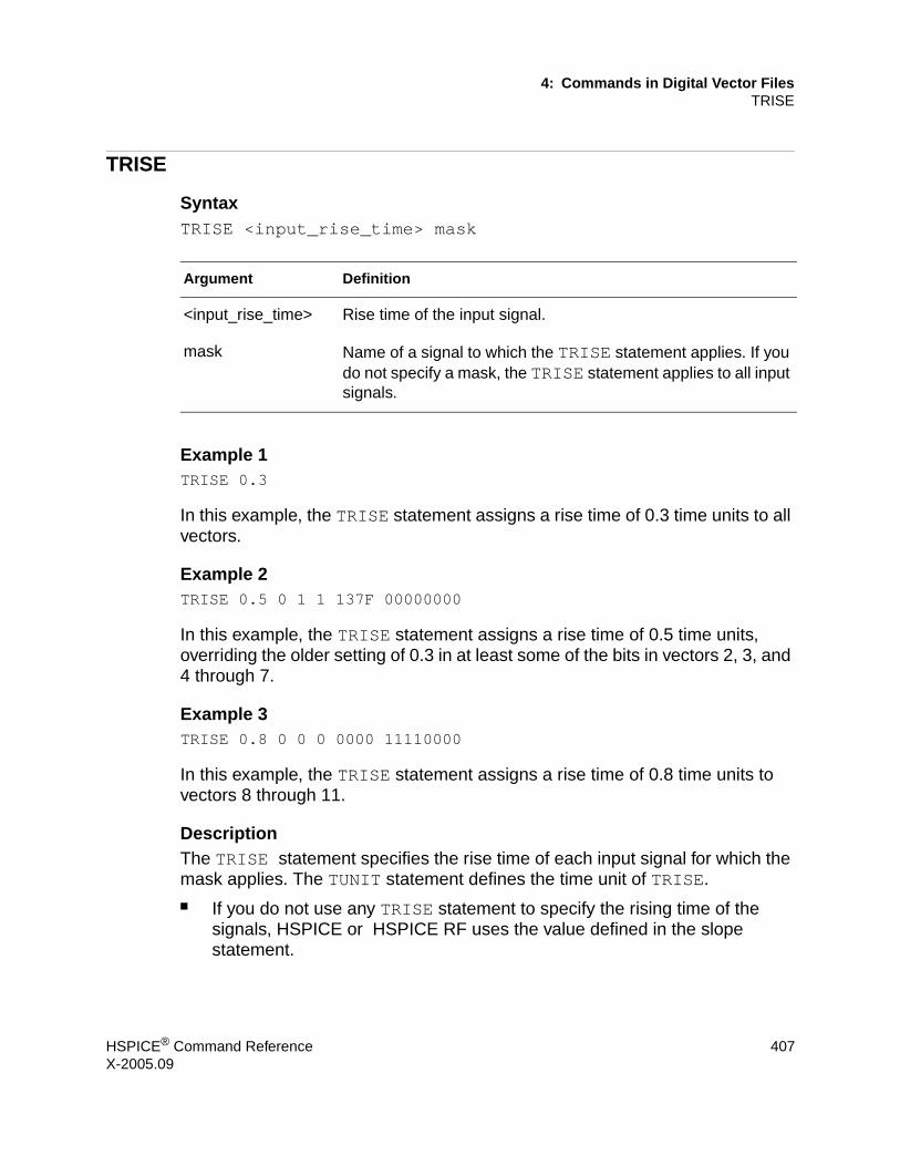
4: Commands in Digital Vector FilesTRISE
TRISE
SyntaxTRISE <input_rise_time> mask
Example 1TRISE 0.3
In this example, the TRISE statement assigns a rise time of 0.3 time units to all vectors.
Example 2TRISE 0.5 0 1 1 137F 00000000
In this example, the TRISE statement assigns a rise time of 0.5 time units, overriding the older setting of 0.3 in at least some of the bits in vectors 2, 3, and 4 through 7.
Example 3TRISE 0.8 0 0 0 0000 11110000
In this example, the TRISE statement assigns a rise time of 0.8 time units to vectors 8 through 11.
DescriptionThe TRISE statement specifies the rise time of each input signal for which the mask applies. The TUNIT statement defines the time unit of TRISE.■ If you do not use any TRISE statement to specify the rising time of the
signals, HSPICE or HSPICE RF uses the value defined in the slope statement.
Argument Definition
<input_rise_time> Rise time of the input signal.
mask Name of a signal to which the TRISE statement applies. If you do not specify a mask, the TRISE statement applies to all input signals.
HSPICE® Command Reference 407X-2005.09

4: Commands in Digital Vector FilesTRISE
■ If you apply more than one TRISE statement to a signal, the last statement overrules the previous statements, and HSPICE or HSPICE RF issues a warning message.
TRISE statements have no effect on the expected output signals.
408 HSPICE® Command ReferenceX-2005.09

4: Commands in Digital Vector FilesTRIZ
TRIZ
SyntaxTRIZ <output_impedance>
ExampleTRIZ 15.1MegTRIZ 150Meg 1 1 1 0000 00000000TRIZ 50.5Meg 0 0 0 137F 00000000
■ The first TRIZ statement sets the high impedance resistance globally, at 15.1 Mohms.
■ The second TRIZ statement increases the value to 150 Mohms, for vectors 1 to 3.
■ The last TRIZ statement increases the value to 50.5 Mohms, for vectors 4 through 7.
DescriptionThe TRIZ statement specifies the output impedance, when the signal (for which the mask applies) is in tristate; TRIZ applies only to the input signals.■ If you do not specify the tristate impedance of a signal, in a TRIZ statement,
HSPICE or HSPICE RF assumes 1000M. ■ If you apply more than one TRIZ statement to a signal, the last statement
overrules the previous statements, and HSPICE or HSPICE RF issues a warning.
TRIZ statements have no effect on the expected output signals.
Argument Definition
<output_impedance> Output impedance of the input signal.
mask Name of a signal to which the TRIZ statement applies. If you do not specify a mask, the TRIZ statement applies to all input signals.
HSPICE® Command Reference 409X-2005.09

4: Commands in Digital Vector FilesTSKIP
TSKIP
SyntaxTSKIP <absolute_time> <tabular_data> ...
Exampleradix 1111 1111period 10tskip11.0 1000 100020.0 1100 110033.0 1010 1001
HSPICE or HSPICE RF ignores the absolute times 11.0, 20.0 and 33.0, but HSPICE does process the tabular data on the same lines as those absolute times.
DescriptionThe TSKIP statement specifies to ignore the absolute time field in the tabular data. You can then keep, but ignore, the absolute time field of each row in the tabular data, when you use the PERIOD statement.
You might do this, for example, if the absolute times are not perfectly periodic for testing reasons. Another reason might be that a path in the circuit does not meet timing, but you might still use it as part of a test bench. Initially, HSPICE or HSPICE RF writes to the vector file, using absolute time. After you fix the circuit, you might want to use periodic data.
Argument Definition
<absolute_time> Absolute time.
<tabular_data> Data captured at <absolute_time>.
410 HSPICE® Command ReferenceX-2005.09
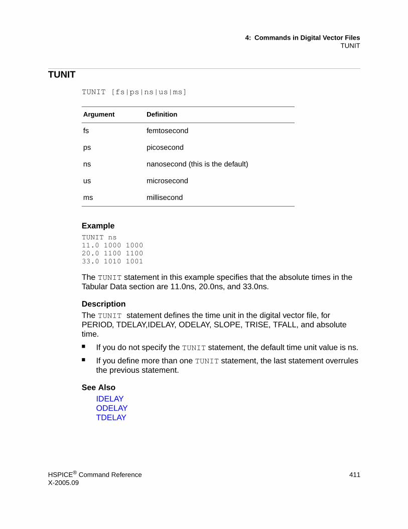
4: Commands in Digital Vector FilesTUNIT
TUNIT
TUNIT [fs|ps|ns|us|ms]
ExampleTUNIT ns11.0 1000 100020.0 1100 110033.0 1010 1001
The TUNIT statement in this example specifies that the absolute times in the Tabular Data section are 11.0ns, 20.0ns, and 33.0ns.
DescriptionThe TUNIT statement defines the time unit in the digital vector file, for PERIOD, TDELAY,IDELAY, ODELAY, SLOPE, TRISE, TFALL, and absolute time. ■ If you do not specify the TUNIT statement, the default time unit value is ns. ■ If you define more than one TUNIT statement, the last statement overrules
the previous statement.
See AlsoIDELAYODELAYTDELAY
Argument Definition
fs femtosecond
ps picosecond
ns nanosecond (this is the default)
us microsecond
ms millisecond
HSPICE® Command Reference 411X-2005.09
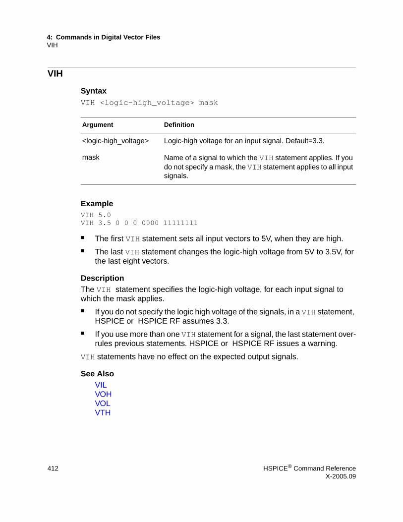
4: Commands in Digital Vector FilesVIH
VIH
SyntaxVIH <logic-high_voltage> mask
ExampleVIH 5.0VIH 3.5 0 0 0 0000 11111111
■ The first VIH statement sets all input vectors to 5V, when they are high. ■ The last VIH statement changes the logic-high voltage from 5V to 3.5V, for
the last eight vectors.
DescriptionThe VIH statement specifies the logic-high voltage, for each input signal to which the mask applies.■ If you do not specify the logic high voltage of the signals, in a VIH statement,
HSPICE or HSPICE RF assumes 3.3. ■ If you use more than one VIH statement for a signal, the last statement over-
rules previous statements. HSPICE or HSPICE RF issues a warning.
VIH statements have no effect on the expected output signals.
See AlsoVILVOHVOLVTH
Argument Definition
<logic-high_voltage> Logic-high voltage for an input signal. Default=3.3.
mask Name of a signal to which the VIH statement applies. If you do not specify a mask, the VIH statement applies to all input signals.
412 HSPICE® Command ReferenceX-2005.09

4: Commands in Digital Vector FilesVIL
VIL
SyntaxVIL <logic-low_voltage>
ExampleVIL 0.0VIL 0.5 0 0 0 0000 11111111
■ The first VIL statement sets the logic-low voltage to 0V, for all vectors. ■ The second VIL statement changes the logic-low voltage to 0.5V, for the last
eight vectors.
DescriptionThe VILstatement specifies the logic-low voltage, for each input signal to which the mask applies.■ If you do not specify the logic-low voltage of the signals, in a VIL statement,
HSPICE or HSPICE RF assumes 0.0. ■ If you use more than one VIL statement for a signal, the last statement over-
rules previous statements. HSPICE or HSPICE RF issues a warning.
VIL statements have no effect on the expected output signals.
See AlsoVIHVOHVOLVTH
Argument Definition
<logic-low_voltage> Logic-low voltage for an input signal. Default=0.0.
mask Name of a signal to which the VIL statement applies. If you do not specify a mask, the VIL statement applies to all input signals.
HSPICE® Command Reference 413X-2005.09

4: Commands in Digital Vector FilesVNAME
VNAME
SyntaxVNAME vector_name[[starting_index : ending_index]]
Example 1RADIX 1 1 1 1 1 1 1 1 1 1 1 1VNAME V1 V2 V3 V4 V5 V6 V7 V8 V9 V10 V11 V12
Example 2VNAME a[[0:3]]
This example represents a0, a1, a2, and a3, in that order. HSPICE or HSPICE RF does not reverse the order to make a3 the first bit.
The bit order is MSB:LSB, which means most significant bit to least significant bit. For example, you can represent a 5-bit bus such as: {a4 a3 a2 a1 a0}, using this notation: a[[4:0]]. The high bit is a4, which represents 24. It is the largest value, and therefore is the MSB.
Example 3RADIX 2 4VNAME VA[[0:1]] VB[[4:1]]
Argument Definition
<vector_name> Name of the vector, or range of vectors.
starting_index First bit in a range of vector names.
ending_index Last bit in a range of vector names. You can associate a single name with multiple bits (such as bus notation).
The opening and closing brackets and the colon are required; they indicate that this is a range. The vector name must correlate with the number of bits available.
You can nest the bus definition inside other grouping symbols, such as {}, (), [], and so on. The bus indices expand in the specified order
414 HSPICE® Command ReferenceX-2005.09

4: Commands in Digital Vector FilesVNAME
HSPICE or HSPICE RF generates voltage sources with the following names:
VA0 VA1 VB4 VB3 VB2 VB1
■ VA0 and VB4 are the MSBs.■ VA1 and VB1 are the LSBs.
Example 4VNAME VA[[0:1]] VB<[4:1]>
HSPICE or HSPICE RF generates voltage sources with the following names:
VA[0] VA[1] VB<4> VB<3> VB<2> VB<1>
Example 5VNAME VA[[2:2]]
This example specifies a single bit of a bus. This range creates a voltage source named:
VA[2]
Example 6RADIX 444444VNAME A[[0:23]]
This example generates signals named A0, A1, A2, ... A23.
DescriptionThe VNAME statement defines the name of each vector. If you do not specify VNAME, HSPICE or HSPICE RF assigns a default name to each signal: V1, V2, V3, and so on. If you define more than one VNAME statement, the last statement overrules the previous statement.
HSPICE® Command Reference 415X-2005.09

4: Commands in Digital Vector FilesVOH
VOH
SyntaxVOH <logic-high_voltage> mask
ExampleVOH 4.75VOH 4.5 1 1 1 137F 00000000VOH 3.5 0 0 0 0000 11111111
■ The first line tries to set a logic-high output voltage of 4.75V, but it is redundant.
■ The second line changes the voltage level to 4.5V, for the first seven vectors. ■ The last line changes the last eight vectors to a 3.5V logic-high output.
These second and third lines completely override the first VOH statement.
If you do not define either VOH or VOL, HSPICE or HSPICE RF uses VTH (default or defined).
DescriptionThe VOH statement specifies the logic-high voltage, for each output signal to which the mask applies.■ If you do not specify the logic-high voltage in a VOH statement, HSPICE or
HSPICE RF assumes 2.64. ■ If you apply more than one VOH statement to a signal, the last statement
overrules the previous statements, and HSPICE or HSPICE RF issues a warning.
VOH statements have no effect on input signals.
Argument Definition
<logic-high_voltage> Logic-high voltage for an output vector. Default=2.66.
mask Name of a signal to which the VOH statement applies. If you do not specify a mask, the VOH statement applies to all output signals.
416 HSPICE® Command ReferenceX-2005.09

4: Commands in Digital Vector FilesVOH
See AlsoVIHVILVOLVTH
HSPICE® Command Reference 417X-2005.09

4: Commands in Digital Vector FilesVOL
VOL
SyntaxVOL <logic-low_voltage> mask
ExampleVOL 0.0VOL 0.2 0 0 0 137F 00000000VOL 0.5 1 1 1 0000 00000000
■ The first VOL statement sets the logic-low output to 0V. ■ The second VOL statement sets the output voltage to 0.2V, for the fourth
through seventh vectors. ■ The last statement increases the voltage further to 0.5V, for the first three
vectors.
These second and third lines completely override the first VOL statement.
If you do not define either VOH or VOL, HSPICE or HSPICE RF uses VTH (default or defined).
DescriptionThe VOL statement specifies the logic-low voltage, for each output signal to which the mask applies.■ If you do not specify the logic-low voltage, in a VOL statement, HSPICE or
HSPICE RF assumes 0.66. ■ If you apply more than one VOL statement to a signal, the last statement
overrules the previous statements, and HSPICE or HSPICE RF issues a warning.
Argument Definition
<logic-low_voltage> Logic-low voltage for an output vector. Default=0.64.
mask Name of a signal to which the VOL statement applies. If you do not specify a mask, the VOL statement applies to all output signals.
418 HSPICE® Command ReferenceX-2005.09

4: Commands in Digital Vector FilesVOL
See AlsoVIHVILVOHVTH
HSPICE® Command Reference 419X-2005.09

4: Commands in Digital Vector FilesVREF
VREF
SyntaxVREF <reference_voltage>
ExampleVNAME v1 v2 v3 v4 v5[[1:0]] v6[[2:0]] v7[[0:3]] v8 v9 v10 VREF 0VREF 0 111 137F 000VREF vss 0 0 0 0000 111
When HSPICE or HSPICE RF implements these statements into the netlist, the voltage source realizes v1:
v1 V1 0 pwl(......)
as well as v2, v3, v4, v5, v6, and v7.
However, v8 is realized by
V8 V8 vss pwl(......)
v9 and v10 use a syntax similar to v8.
DescriptionSimilar to the TDELAY statement, the VREF statement specifies the name of the reference voltage, for each input vector to which the mask applies. VREF applies only to input signals.■ If you do not specify the reference voltage name of the signals, in a VREF
statement, HSPICE or HSPICE RF assumes 0.■ If you apply more than one VREF statement, the last statement overrules the
previous statements, and HSPICE or HSPICE RF issues a warning.
VREF statements have no effect on the output signals.
Argument Definition
<reference_voltage> Reference voltage for each input vector. Default=0.
420 HSPICE® Command ReferenceX-2005.09

4: Commands in Digital Vector FilesVTH
VTH
SyntaxVTH <logic-threshold_voltage>
ExampleVTH 1.75VTH 2.5 1 1 1 137F 00000000VTH 1.75 0 0 0 0000 11111111
■ The first VTH statement sets the logic threshold voltage at 1.75V. ■ The next line changes that threshold to 2.5V, for the first 7 vectors. ■ The last line changes that threshold to 1.75V, for the last 8 vectors.
All of these examples apply the same vector pattern, and both output and input control statements, so the vectors are all bidirectional.
DescriptionSimilar to the TDELAY statement, the VTH statement specifies the logic threshold voltage, for each output signal to which the mask applies. The threshold voltage determines the logic state of output signals, for comparison with the expected output signals.■ If you do not specify the threshold voltage of the signals, in a VTH statement,
HSPICE or HSPICE RF assumes 1.65.■ If you apply more than one VTH statement to a signal, the last statement
overrules the previous statements, and HSPICE or HSPICE RF issues a warning.
VTH statements have no effect on the input signals.
Argument Definition
<logic-threshold_voltage> Logic-threshold voltage for an output vector. Default=1.65.
HSPICE® Command Reference 421X-2005.09

4: Commands in Digital Vector FilesVTH
See AlsoVIHVILVOHVOL
422 HSPICE® Command ReferenceX-2005.09
Index
AABSH option 195ABSI option 196, 286ABSMOS option 197, 286ABSTOL option 198ABSV option 199ABSVAR option 200ABSVDC option 201AC analysis
magnitude 204optimization 9output 204phase 204
.AC command 9external data 29
ACCURATE option 203ACOUT option 204algorithms
DVDT 200, 292local truncation error 292, 342, 368pivoting 325timestep control 254transient analysis timestep 292trapezoidal integration 303
.ALIAS command 14ALL keyword 134, 158ALT9999 option 205ALTCC option 206ALTCHK option 207alter block commands 1.ALTER command 16, 44Analog Artist interface 336
See also ArtistAnalysis commands 1analysis, network 129arithmetic expression 111
ARTIST option 208, 336ASCII output data 221, 301, 355ASPEC option 209AT keyword 109autoconvergence 238AUTOSTOP option 210average measurements, with .MEASURE 105average nodal voltage, with .MEASURE 112average value, measuring 112AVG keyword 113
BBADCHR option 211, 212BETA keyword 156.BIASCHK command 18BIASFILE option 213BIAWARN option 214BINPRINT option 215bisection
pushout 121BKPSIZ option 216branch current error 196breakpoint table, size 216BRIEF option 134, 135, 217, 291, 309, 318, 322BSIM model, LEVEL 13 128BSIM2 model, LEVEL 39 128bus notation 414BYPASS option 218BYTOL option 219
CCadence
Opus 221, 355WSF format 221, 355
HSPICE® Command Reference 423X-2005.09

IndexC
capacitancecharge tolerance, setting 222CSHUNT node-to-ground 229table of values 220
capacitor, models 124CAPTAB option 220CDS option 221CENDIF optimization parameter 125characterization of models 35charge tolerance, setting 222CHGTOL option 222CLOSE optimization parameter 125CMIFLAG option 223CO option 181, 186, 224column laminated data 28commands
.AC 9
.ALIAS 14
.ALTER 16, 44alter block 1analysis 1.BIASCHK 18.CONNECT 23.DATA 25.DC 32.DCMATCH 38.DCVOLT 40.DEL LIB 42.DISTO 46.DOUT 49.EBD 52.ELSE 54.ELSEIF 55.END 56.ENDDATA 57.ENDIF 58.ENDL 59.ENDS 60.EOM 61.FFT 62.FOUR 65.FSOPTIONS 66.GLOBAL 68.GRAPH 69.HDL 71.IBIS 72.IC 76.ICM 78
.IF 79
.INCLUDE 81
.LAYERSTACK 82
.LIB 84
.LOAD 91
.MACRO 93
.MALIAS 96
.MATERIAL 98
.MEASURE 100
.MODEL 123
.NET 129
.NODESET 131
.NOISE 132
.OP 133
.PARAM 137
.PAT 141
.PKG 143
.PLOT 145
.PRINT 147
.PROBE 151
.PROTECT 153
.PZ 154
.SAVE 157
.SENS 159
.SHAPE 161
.STIM 167subcircuit 5.SUBCKT 172.TEMP 175.TF 177.TITLE 178.TRAN 179.UNPROTECT 184.VEC 185Verilog-A 5.WIDTH 186
Common Simulation Data Format 252concatenated data files 27Conditional Block 2conductance
current source, initialization 265minimum, setting 266models 239MOSFETs 267negative, logging 251node-to-ground 270sweeping 268
.CONNECT command 23
424 HSPICE® Command ReferenceX-2005.09

IndexD
control optionsprinting 322setting 135transient analysis
limit 372CONVERGE option 225, 240convergence
for optimization 127problems
causes 218changing integration algorithm 303CONVERGE option 225, 240DCON setting 238decreasing the timestep 261.NODESET statement 131nonconvergent node listing 238operating point Debug mode 134setting DCON 238
steady state 268CPTIME option 226CPU time, reducing 310CROSS keyword 108CSDF option 227CSHDC option 228CSHUNT option 229current
ABSMOS floor value for convergence 341branch 196operating point table 134
CURRENT keyword 134CUSTCMI option 230CUT optimization parameter 125CVTOL option 231
DD_IBIS option 232.DATA command 25, 26
datanames 29external file 25for sweep data 29inline data 29
data files, disabling printout 217, 318DATA keyword 11, 28, 35, 181datanames 29, 169DC
analysisdecade variation 36
initialization 236iteration limit 278linear variation 36list of points 36octave variation 36
optimization 32.DC command 32, 35
external data with .DATA 29DCAP option 233DCCAP option 234DCFOR option 235DCHOLD option 236DCIC option 237.DCMATCH command 38DCON option 238DCSTEP option 239DCTRAN option 240.DCVOLT command 40, 76DEBUG keyword 134DEC keyword 12, 36, 182DEFAD option 241DEFAS option 242DEFL option 243DEFNRD option 244DEFNRS option 245DEFPD option 246DEFPS option 247DEFW option 248.DEL LIB command 42
with .ALTER 44with .LIB 44
delaysgroup 369
DELMAX option 249, 349DELTA internal timestep 249
See also timestepderivative function 116DERIVATIVE keyword 117derivatives, measuring 108DI option 250DIAGNOSTIC option 251DIFSIZ optimization parameters 126DIM2 distortion measure 47DIM3 distortion measure 47diode models 124.DISTO command 46
HSPICE® Command Reference 425X-2005.09

IndexE
distortionHD2 47HD3 48
distortion measuresDIM2 47DIM3 47
DLENCSDF option 252.DOUT command 49DV option 238, 253DVDT
algorithm 200, 345option 254, 292
DVDT option 254DVTR option 255
E.EBD command 52element
checking, suppression of 310OFF parameter 319
.ELSE command 54
.ELSE statement 54
.ELSEIF command 55Encryption 2.END command 56
for multiple HSPICE runs 56location 56
.ENDDATA command 57ENDDATA keyword 25, 27, 30.ENDIF command 58.ENDL command 59, 86.ENDS command 60.EOM command 61EPSMIN option 256equation 111ERR function 119ERR1 function 119ERR2 function 119ERR3 function 119error function 119errors
branch current 196function 119internal timestep too small 229, 350optimization goal 103tolerances
ABSMOS 197branch current 196RELMOS 197voltage 343, 344, 346
example, subcircuit test 93, 172EXPLI option 257EXPMAX option 258expression, arithmetic 111external data files 30
FFALL keyword 108FAST option 259.FFT command 62FFTOUT option 260FIL keyword 30files
column lamination 28concatenated data files 27filenames 30hspice.ini 301include files 81, 85multiple simulation runs 56
FIND keyword 108FIND, using with .MEASURE 107floating point overflow
CONVERGE setting 225setting GMINDC 267
.FOUR command 65frequency
ratio 47sweep 10
FROM parameter 120FS option 156, 261.FSOPTIONS command 66FT option 262functions
ERR 119ERR1 119ERR2 119ERR3 119error 119
GGDCPATH option 263GENK option 264
426 HSPICE® Command ReferenceX-2005.09

IndexH
.GLOBAL command 68global node names 68GMAX option 265GMIN option 266, 267GMINDC option 267GOAL keyword 113GRAD optimization parameter 126GRAMP
calculation 238option 268
.GRAPH command 69graph data file (Viewlogic format) 252group delay, calculating 369GSHDC option 269GSHUNT option 270
HH9007 option 271harmonic distortion 47HD2 distortion 47HD3 distortion 48.HDL command 71HIER_SCALE option 272HSPICE
job statistics report ??–202version
H9007 compatibility 271parameter 128
hspice.ini file 301
I.IBIS command 72IBIS commands 3.IC command 40, 76
from .SAVE 157IC parameter 40, 76, 157.ICM command 78ICSWEEP option 273.IF command 79IGNOR keyword 119IMAX option 274, 281IMIN option 275, 280.INCLUDE command 81include files 81, 85indepout 169
indepvar 169, 170inductors, mutual model 124INGOLD option 276, 297initial conditions
saving and reusing 273transient 182
initialization 319inline data 29inner sweep 26input
dataadding library data 44column laminated 28concatenated data files 27deleting library data 44external, with .DATA statement 29filenames on networks 28formats 28, 29include files 81printing 291suppressing printout 291
netlist file 56INTEG keyword 113, 115
used with .MEASURE 112integral function 115integration
backward Euler method 294order of 294
interfacesAnalog Artist 336Mentor 302MSPICE 302ZUKEN 379
intermodulation distortion 47INTERP option 277iterations
limit 278maximum number of 282
ITL1 option 278ITL2 option 279ITL3 option 280ITL4 option 281ITL5 option 282ITLPTRAN option 283ITLPZ option 284ITROPT optimization parameter 126ITRPRT option 285
HSPICE® Command Reference 427X-2005.09

IndexJ
JJacobian data, printing 321
KKCLTEST option 286keywords
.AC statement parameter 11ALL 134, 158AT 109AVG 113BETA 156CROSS 108CURRENT 134DATA 11, 28, 35, 181.DATA command parameter 28.DC command parameter 35DEBUG 134DEC 12, 36, 182DERIVATIVE 117ENDDATA 25, 27, 30FALL 108FIL 30FIND 108FS 156IGNOR 119INTEG 112, 113, 115LAM 28, 30LAST 109LIN 12, 36, 182MAXFLD 156.MEASUREMENT command parameter 113MER 27, 28, 30MINVAL 120MODEL 35.MODEL statement parameters 123MONTE 12, 181NONE 134, 158NUMF 156OCT 12, 36, 182OPTIMIZE 35PLOT 123POI 12, 36, 182PP 112, 113RESULTS 35RIN 130RISE 108START 182
SWEEP 12, 36, 182target syntax 109TO 113, 120TOL 156TOP 158.TRAN command parameter 181TRIG 101VOLTAGE 134WEIGHT 113, 120weight 113WHEN 108
Kirchhoff’s Current Law (KCL) test 286KLIM option 287
LLAM keyword 28, 30laminated data 28LAST keyword 109latent devices
BYPASS option 218excluding 259
.LAYERSTACK command 82LENNAM option 288LEVEL 13 BSIM model 128LEVEL parameter 126.LIB command 84
call statement 86in .ALTER blocks 86nesting 86with .DEL LIB 44
librariesadding with .LIB 44building 86DDL 356defining macros 86deleting 42private 153protecting 153
Library Management 3LIMPTS option 289LIMTIM option 290LIN keyword 12, 36, 182LIST option 291listing, suppressing 153.LOAD command 91local truncation error algorithm 292, 342, 368
428 HSPICE® Command ReferenceX-2005.09
IndexM
LVLTIM option 292, 303, 345, 368
M.MACRO command 93macros 44, 86magnetic core models 124.MALIAS command 96.MATERIAL command 98Material Properties 3matrix
minimum pivot values 329parameters 129row/matrix ratio 328size limitation 327
MAX 112MAX parameter 113, 126MAXAMP option 293MAXFLD keyword 156maximum value, measuring 112MAXORD option 294MBYPASS option 295MCBRIEF option 296MEASDGT option 297MEASFAIL option 298MEASFILE option 299MEASOUT option 301MEASSORT option 300.MEASURE command 100, 297, 301
average measurements 105average nodal voltage 112expression 111propogation delay 101
measuring average values 112measuring derivatives 108Mentor interface 302MENTOR option 302MER keyword 27, 28, 30messages
See also errors, warningsmessages, pivot change 326METHOD option 303MIN 112MIN parameter 113minimum value, measuring 112MINVAL keyword 120
.MODEL command 123CENDIF 125CLOSE 125CUT 125DEV 125DIFSIZ 126distribution 126GRAD 126HSPICE version parameter 128ITROPT 126keyword 126LEVEL 126LOT 126MAX 126model name 124PARMIN 127PLOT 127RELIN 127RELOUT 127type 124VERSION 128
MODEL keyword 35model parameters
LEVEL 126suppressing printout of 312TEMP 176
modelsBJTs 124BSIM LEVEL 13 128BSIM2 LEVEL 39 128capacitors 124characterization 35diode 124JFETs 124magnetic core 124MOSFETs 124mutual inductors 124names 124npn BJT 124op-amps 124optimization 124plot 124private 153protecting 153simulator access 86types 124
models, diode 124MODMONTE option 304
HSPICE® Command Reference 429X-2005.09

IndexN
MODSRH option 305Monte Carlo
AC analysis 10DC analysis 32.MODEL parameters 126time analysis 180
MONTE keyword 12, 181MONTECON option 306MSPICE simulator interface 302MU option 307
Nnamei 168, 169, 170n-channel, MOSFET’s models 124negative conductance, logging 251nested library calls 86.NET comamnd 129network
analysis 129filenames 28
network analysis 129NEWTOL option 308Node Naming 4NODE option 309nodes
cross-reference table 309global versus local 68printing 309
.NODESET command 131, 235DC operating point initialization 131from .SAVE 157
NODESET keyword 157node-to-element list 326NOELCK option 310noise
folding 156numerical 229sampling 156
.NOISE command 132NOISEMINFREQ option 311NOMOD option 312NONE keyword 134, 158NOPAGE option 313NOPIV option 314NOTOP option 315NOWARN option 316
npn BJT models 124npoints 168, 169, 170NUMDGT option 317numerical integration algorithms 303numerical noise 229, 270NUMF keyword 156NXX option 318
OOCT keyword 12, 36, 182OFF option 319.OP command 133op-amps model, names 124operating point
capacitance 220.IC statement initialization 40, 76.NODESET statement initialization 131restoring 92solution 319voltage table 134
OPFILE option 320optimization
AC analysis 9algorithm 126DC analysis 32error function 103iterations 126models 124time
analysis 180required 125
optimization parameter, DIFSIZ 126OPTIMIZE keyword 35.OPTION 135
SEARCH 356.OPTION ABSH 195.OPTION ABSI 196.OPTION ABSMOS 197.OPTION ABSTOL 198.OPTION ABSV 199.OPTION ABSVAR 200.OPTION ABSVDC 201.OPTION ACCT 201.OPTION ACCURATE 203.OPTION ACOUT 204.OPTION ALT999 203
430 HSPICE® Command ReferenceX-2005.09
IndexO
.OPTION ALT9999 205
.OPTION ALTCC 206
.OPTION ALTCHK 207
.OPTION ARTIST 208, 336
.OPTION ASPEC 209
.OPTION AUTOSTOP 210
.OPTION BADCHR 211, 212
.OPTION BIASFILE 213
.OPTION BIAWARN 214
.OPTION BINPRINT 215
.OPTION BKPSIZ 216
.OPTION BRIEF 134, 135, 217, 291, 309, 318, 322.OPTION BYPASS 218.OPTION BYTOL 219.OPTION CAPTAB 220.OPTION CDS 221.OPTION CHGTOL 222.OPTION CMIFLAG 223.OPTION CO 181, 186, 224.OPTION CONVERGE 225.OPTION CPTIME 226.OPTION CSDF 227.OPTION CSHDC 228.OPTION CSHUNT 229.OPTION CUSTCMI 230.OPTION CVTOL 231.OPTION D_IBIS 232.OPTION DCAP 233.OPTION DCCAP 234.OPTION DCFOR 235.OPTION DCHOLD 236.OPTION DCIC 237.OPTION DCON 238.OPTION DCSTEP 239.OPTION DCTRAN 240.OPTION DEFAD 241.OPTION DEFAS 242.OPTION DEFL 243.OPTION DEFNRD 244.OPTION DEFNRS 245.OPTION DEFPD 246.OPTION DEFPS 247.OPTION DEFW 248.OPTION DELMAX 249
.OPTION DI 250
.OPTION DIAGNOSTIC 251
.OPTION DLENCSDF 252
.OPTION DV 253
.OPTION DVDT 254
.OPTION DVTR 255
.OPTION EPSMIN 256
.OPTION EXPLI 257
.OPTION EXPMAX 258
.OPTION FAST 259
.OPTION FFTOUT 260
.OPTION FS 261
.OPTION FT 262
.OPTION GDCPATH 263
.OPTION GENK 264
.OPTION GMAX 265
.OPTION GMIN 266
.OPTION GMINDC 267
.OPTION GRAMP 268
.OPTION GSHDC 269
.OPTION GSHUNT 270
.OPTION H9007 271
.OPTION HIER_SCALE 272
.OPTION ICSWEEP 273
.OPTION IMAX 274
.OPTION IMIN 275
.OPTION INGOLD 276
.OPTION INTERP 277
.OPTION ITL1 278
.OPTION ITL2 279
.OPTION ITL3 280
.OPTION ITL4 281
.OPTION ITL5 282
.OPTION ITLPTRAN 283
.OPTION ITLPZ 284
.OPTION ITRPRT 285
.OPTION KCLTEST 286
.OPTION KLIM 287
.OPTION LENNAM 288
.OPTION LIMPTS 289
.OPTION LIMTIM 290
.OPTION LIST 291
.OPTION LVLTIM 292
.OPTION MAXAMP 293
.OPTION MAXORD 294
HSPICE® Command Reference 431X-2005.09
IndexO
.OPTION MBYPASS 295
.OPTION MCBRIEF 296
.OPTION MEASDGT 297
.OPTION MEASFAIL 298
.OPTION MEASFILE 299
.OPTION MEASOUT 301
.OPTION MEASSORT 300
.OPTION MENTOR 302
.OPTION METHOD 303
.OPTION MODMONTE 304
.OPTION MODSRH 305
.OPTION MONTECON 306
.OPTION MU 307
.OPTION NEWTOL 308
.OPTION NODE 309
.OPTION NOELCK 310
.OPTION NOISEMINFREQ 311
.OPTION NOMOD 312
.OPTION NOPAGE 313
.OPTION NOPIV 314
.OPTION NOTOP 315
.OPTION NOWARN 316
.OPTION NUMDGT 317
.OPTION NXX 318
.OPTION OFF 319
.OPTION OPFILE 320
.OPTION OPTLST 321
.OPTION OPTS 322
.OPTION PARHIER 323
.OPTION PATHNUM 324
.OPTION PIVOT 325
.OPTION PIVREF 327
.OPTION PIVREL 328
.OPTION PIVTOL 329
.OPTION PLIM 330
.OPTION POST 331
.OPTION POST_VERSION 333
.OPTION POSTTOP 334
.OPTION PROBE 335
.OPTION PSF 336
.OPTION PURETP 337
.OPTION PUTMEAS 338
.OPTION RELH 339
.OPTION RELI 340
.OPTION RELMOS 341
.OPTION RELQ 342
.OPTION RELTOL 343
.OPTION RELV 344
.OPTION RELVAR 345
.OPTION RELVDC 346
.OPTION RESMIN 347
.OPTION RMAX 349
.OPTION RMIN 350
.OPTION RUNLVL 351
.OPTION SCALE 353
.OPTION SCALM 354
.OPTION SDA 355
.OPTION SEARCH 356
.OPTION SEED 357
.OPTION SLOPETOL 358
.OPTION SPARSE 359
.OPTION SPICE 360
.OPTION SPMODEL 361
.OPTION STATFL 362
.OPTION SYMB 363
.OPTION TIMERES 364
.OPTION TNOM 365
.OPTION TRCON 366
.OPTION TRTOL 368
.OPTION UNWRAP 369
.OPTION VAMODEL 370
.OPTION VERIFY 371
.OPTION VFLOOR 372
.OPTION VNTOL 373
.OPTION WACC 374
.OPTION WARNLIMIT 376
.OPTION WL 377
.OPTION WNFLAG 375
.OPTION XDTEMP 378
.OPTION ZUKEN 379OPTLST option 321OPTS option 322Opus 221, 355oscillation, eliminating 303outer sweep 26Output 4output
dataformat 297, 336limiting 277
432 HSPICE® Command ReferenceX-2005.09
IndexP
significant digits specification 317specifying 289storing 301
filesreducing size of 376
.MEASURE results 100plotting 145printing 147–150printout format 276variables
printing 285probing 151specifying significant digits for 317
ovari 168, 170
P.PARAM command 137parameters
AC sweep 9DC sweep 32defaults 323FROM 120IC 40, 76inheritance 323ITROPT optimization 126LEVEL 126matrix 129names
.MODEL commandparameter name 127
simulator access 86skew, assigning 85UIC 40, 76
PARHIER option 323PARMIN optimization parameter 127.PAT command 141path names 324path numbers, printing 324PATHNUM option 324p-channel
JFETs models 124MOSFET’s models 124
Peak 105peak measurement 105peak-to-peak value 115
measuring 112PERIOD statement 401, 411
pivotalgorithm, selecting 325change message 326reference 327
PIVOT option 325PIVREF option 327PIVREL option 328PIVTOL option 325, 329.PKG command 143PLIM option 330plot
models 124value calculation method 204
.PLOT command 145in .ALTER block 16
PLOT keyword 123pnp BJT models 124POI keyword 12, 36, 182pole/zero analysis, maximum iterations 284polygon, defining 166POST_VERSION option 333POSTTOP option 334power operating point table 134PP 112, 115PP keyword 112, 113.PRINT command 147
in .ALTER 16printing
Jacobian data 321printout
disabling 217, 318suppressing 153value calculation method 204
.PROBE command 151PROBE option 335propogation delays
measuring 102with .MEASURE 101
.PROTECT command 153protecting data 153PSF option 336PURETP option 337pushout bisection 121PUTMEAS option 338.PZ command 154
HSPICE® Command Reference 433X-2005.09

IndexR
Rreference temperature 176RELH option 339RELI option 286, 340RELIN optimization parameter 127RELMOS option 197, 286, 341RELOUT optimization parameter 127RELQ option 342RELTOL option 222, 343RELTOLoption 343RELV option 259, 295, 344RELVAR option 345RELVDC option 344, 346resistance 347RESMIN option 347RESULTS keyword 35RIN keyword 130Rise 101rise and fall times 102RISE keyword 108rise time
specify 406, 407RISETIME option 348RMAX option 349RMIN option 350RMS
measurement 105used with .MEASURE 105
RMS keyword 113ROUT keyword 130row/matrix ratio 328RUNLVL option 351
SS parameter, model type 124.SAMPLE 156.SAMPLE statement 156sampling noise 156.SAVE command 157SCALE option 353SCALM option 354Schmitt trigger example 34SDA option 355SEARCH option 356
SEED option 357.SENS command 159Setup 4.SHAPE command 161
Defining Circles 163Defining Polygons 164Defining Rectangles 162Defining Strip Polygons 166
SIM2 distortion measure 48simulation
accuracy 203, 292improvement 254
multiple analyses, .ALTER statement 16multiple runs 56reducing time 29, 210, 218, 254, 275, 280,
358, 368results
plotting 145printing 147specifying 100
title 178Simulation Runs 5skew, parameters 85SLOPE statement 411SLOPETOL option 358small-signal, DC sensitivity 159source
AC sweep 9DC sweep 32
SPARSE option 359SPICE
compatibility 360AC output 204plot 330
SPICE option 360SPMODEL option 361START keyword 182statement
PERIOD 401, 411SLOPE 411TDELAY 411TFALL 411TRISE 411TSKIP 401TUNIT, with TRISE statement 406, 407
statements.AC 9.ALIAS 14
434 HSPICE® Command ReferenceX-2005.09

IndexT
.ALTER 16, 44alter block 1.BIASCHK 18.CONNECT 23.DATA 25
external file 25inline 25
.DC 32, 35
.DCMATCH 38
.DCVOLT 40, 76
.DEL LIB 42
.DISTO 46
.DOUT 49
.EBD 52
.ELSE 54
.ELSEIF 55
.END 56
.ENDDATA 57
.ENDIF 58
.ENDL 59, 86
.ENDS 60, 61
.EOM 61
.FFT 62
.FOUR 65
.FSOPTIONS 66
.GLOBAL 68
.GRAPH 69
.HDL 71
.IBIS 72
.IC 40, 76
.ICM 78
.IF 79
.INCLUDE 54, 56, 79, 81, 157
.LAYERSTACK 82
.LIB 84, 86nesting 86
.LOAD 91
.MACRO 93
.MALIAS 96
.MATERIAL 98
.MEASURE 100, 297, 301
.MODEL 123
.NET 129
.NODESET 131, 235
.NOISE 132
.OP 133
.OPTION SEARCH 356
.PARAM 137
.PAT 141
.PKG 143
.PLOT 145
.PRINT 147
.PROBE 151
.PROTECT 153
.PZ 154
.SAMPLE 156
.SAVE 157
.SENS 159
.SHAPE 161
.STIM 167
.SUBCKT 172
.TEMP 175, 176
.TF 177
.TITLE 178
.TRAN 179
.UNPROTECT 184
.VEC 185
.WIDTH 186STATFL option 362statistics, listing 202steatements
.ELSE 54.STIM command 167subcircuit commands 5subcircuits
calling 93, 172global versus local nodes 68names 94, 174node numbers 94, 174parameter 60, 61, 93, 94, 172, 174printing path numbers 324test example 93, 172
.SUBCKT command 172sweep
data 26, 301frequency 10inner 26outer 26
SWEEP keyword 12, 36, 182SYMB option 363
TTabular Data section
time interval 401TARG_SPEC 101
HSPICE® Command Reference 435X-2005.09

IndexU
target specification 102TDELAY statement 411TEMP
keyword 12, 36model parameter 176
.TEMP command 175temperature
AC sweep 9DC sweep 32, 33derating 176reference 176
.TF command 177TFALL statement 411threshold voltage 49time 134
See also CPU timeTIMERES option 364timestep
algorithms 254calculation for DVDT=3 261changing size 342control 261, 345, 368internal 249maximum 274, 281, 349minimum 275, 280, 350reversal 200setting initial 249transient analysis algorithm 292variation by HSPICE 249
.TITLE command 178title for simulation 178TNOM option 176, 365TO keyword 113, 120TOL keyword 156TOP keyword 158.TRAN command 179transient analysis
Fourier analysis 65initial conditions 40, 76number of iterations 282
TRAP algorithmSee trapezoidal integration
trapezoidal integrationcoefficient 307
TRCON option 366TRIG keyword 101TRIG_SPEC 101trigger specification 102
TRISE statement 406, 407, 411TRTOL option 368TSKIP statement 401TSTEP
multiplier 349, 350option 349, 350
TUNIT statement 411with TRISE statement 406, 407
UU Element, transmission line model 124UIC
keyword 182parameter 40, 76
.UNPROTECT command 184UNWRAP option 369
VVAMODEL option 370.VEC command 185VERIFY option 371Verilog-A commands 5version
H9007 compatibility 271HSPICE 128
Version Options 369, 370VFLOOR option 372Viewlogic graph data file 252VIH statement 412VIL statement 413VNTOL option 259, 373VOH statement 416, 418voltage
error toleranceDC analysis 344, 346transient analysis 343
initial conditions 40, 76iteration-to-iteration change 253logic high 412, 416, 418logic low 413maximum change 200minimum
DC analysis 201listing 372transient analysis 199
operating point table 134
436 HSPICE® Command ReferenceX-2005.09

IndexW
relative change, setting 345tolerance
MBYPASS multiplier 295value for BYPASS 219
VOLTAGE keyword 134VREF statement 420VTH statement 421
WW Elements transmission line model 124WACC option 374warnings
limiting repetitions 376misuse of VERSION parameter 128suppressing 316
WARNLIMIT option 376WEIGHT keyword 113, 120
WHEN keyword 108WHEN, using with .MEASURE 107.WIDTH command 186WL option 377WNFLAG option 375WSF output data 221, 355
XXDTEMP option 378
YYMAX parameter 120YMIN parameter 119
ZZUKEN option 379
HSPICE® Command Reference 437X-2005.09

IndexZ
438 HSPICE® Command ReferenceX-2005.09


