The Impact of Basel Accords on the Lender's Profitability under Different Pricing Decisions Bo Huang; Prof Lyn Thomas School of Management, University of Southampton Credit Scoring and Credit Control XII conference August 24-26 /2011 1
Transcript
The Impact of Basel Accords on the Lender's Profitability under Different Pricing Decisions
Bo Huang; Prof Lyn Thomas
School of Management, University of Southampton
Credit Scoring and Credit Control XII conference
August 24-26 /2011
1
Aim of Project • Understand the influence of different Basel regulations on pricing decisions
the lender has an agreed cost of equity for each unit of equity needed to cover the regulatory capital requirement.
the lender decides in advance how much of its equity capital can be set aside to cover the requirements of this loan portfolio.
2
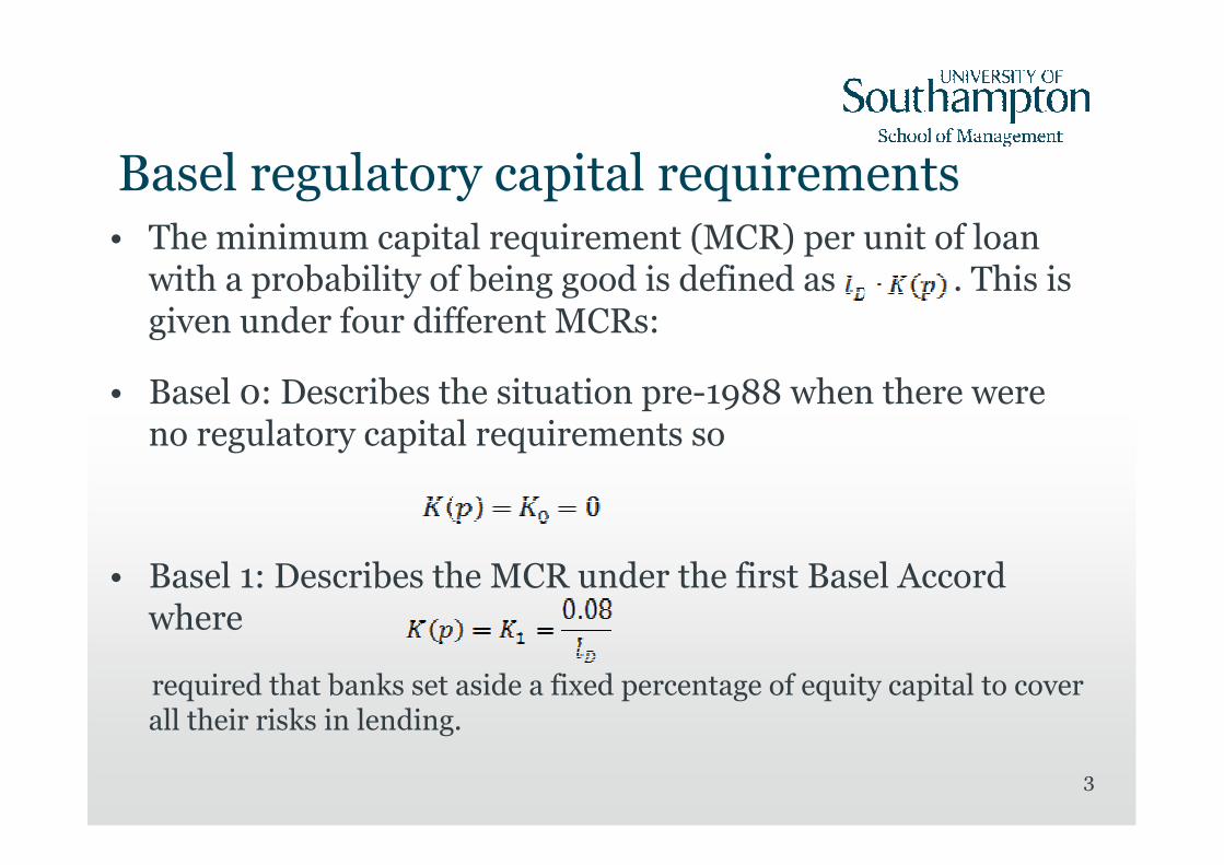
Basel regulatory capital requirements • The minimum capital requirement (MCR) per unit of loan with a probability of being good is defined as . This is given under four different MCRs:
• Basel 0: Describes the situation pre-1988 when there were no regulatory capital requirements so
• Basel 1: Describes the MCR under the first Basel Accord where
required that banks set aside a fixed percentage of equity capital to cover all their risks in lending.
3
• Basel 2: Describes the MCR under the second Basel Accord where
where (credit cards)
The capital requirement in Basel 2 was taken as 8% of the risk weighted assets to
have the same terminology as Basel 1, where the risk weighted assets were given by a function of the probability of default of the loans.
• Basel 3: the MCR for the third of Basel Accord can be written as:
Basel 3 tightens up what is required as capital, introduces liquidity requirements,
and increases the capital requirement by factoring up the capital requirements of Basel 2.
4
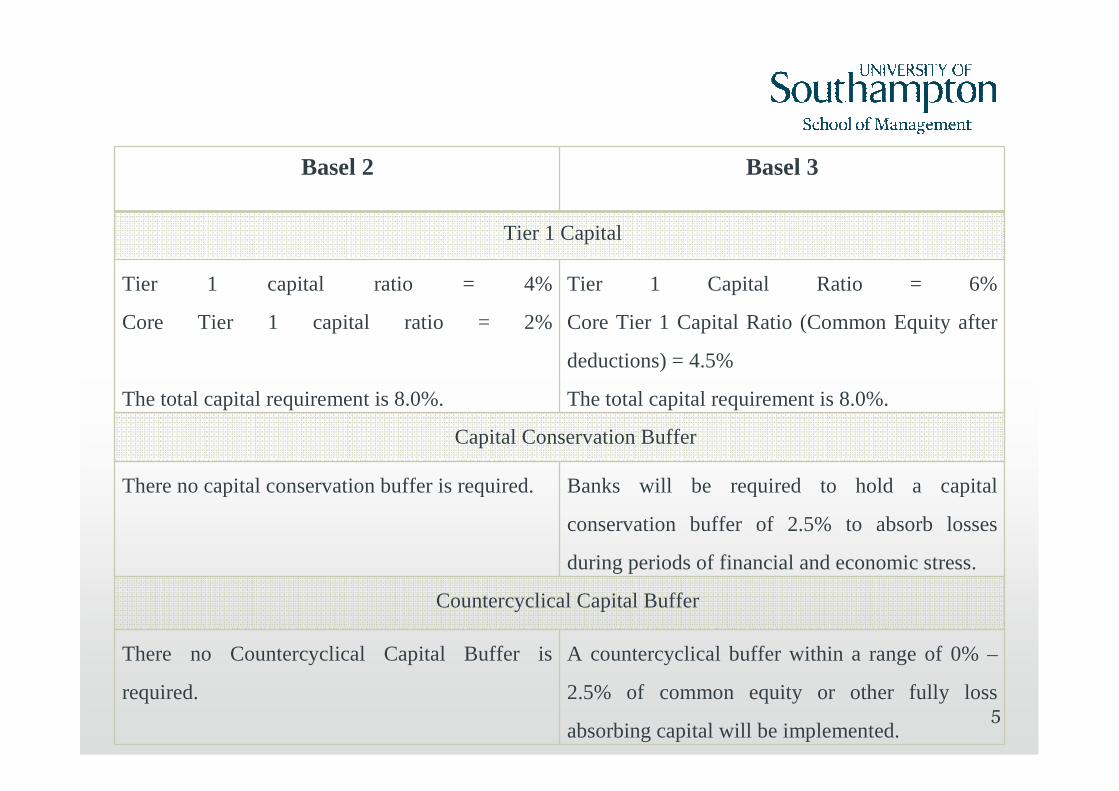
Basel 2 Basel 3
Tier 1 Capital
Tier 1 capital ratio = 4%
Core Tier 1 capital ratio = 2%
The total capital requirement is 8.0%.
Tier 1 Capital Ratio = 6%
Core Tier 1 Capital Ratio (Common Equity after
deductions) = 4.5%
The total capital requirement is 8.0%.
Capital Conservation Buffer
There no capital conservation buffer is required. Banks will be required to hold a capital
conservation buffer of 2.5% to absorb losses
during periods of financial and economic stress.
Countercyclical Capital Buffer
There no Countercyclical Capital Buffer is
required.
A countercyclical buffer within a range of 0% –
2.5% of common equity or other fully loss
absorbing capital will be implemented.5
General Model • We assume the probability p of the borrowers being good has uniform distribution. Thus the probability density function is , so no one with probability of being good less than a is in the potential borrowers’ population.
• We now consider the portfolio where 1 unit is available to be lent over the whole portfolio.
• : loss given default.
• : rate of which lenders borrow money.
• : rate of return required by equity owner.
• Let B denote the sum of the cost of the regulatory capital and the risk free rate .
• take probability which is percentage of borrowers with probability p of being good who take loan with interest rate r.
1,1
1)( ≤≤
−= pa
apf
Dl
Fr
Qr
),( prq
6
)( pklr DQ ⋅⋅Fr
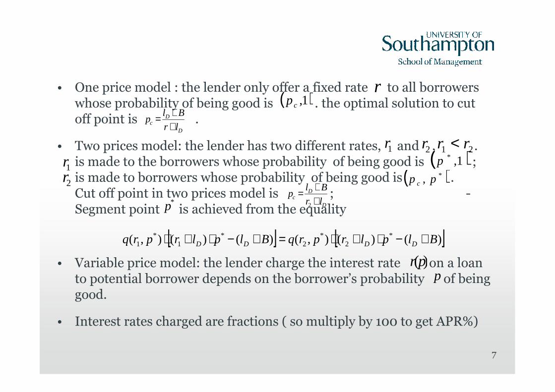
• One price model : the lender only offer a fixed rate to all borrowers whose probability of being good is . the optimal solution to cut off point is .
• Two prices model: the lender has two different rates, and , . is made to the borrowers whose probability of being good is ; is made to borrowers whose probability of being good is . Cut off point in two prices model is ; -Segment point is achieved from the equality
• Variable price model: the lender charge the interest rate on a loan to potential borrower depends on the borrower’s probability of being good.
• Interest rates charged are fractions ( so multiply by 100 to get APR%)
[ ] [ ])()(),()()(),( *2
*2
*1
*1 BlplrprqBlplrprq DDDD +−⋅+⋅=+−⋅+⋅
D
Dc lr
Blp
++=
2
( )*, pp c
( )1,*p21 rr <1r 2r
( )1,cpr
D
Dc lr
Blp
++=
p)(pr
7
1r2r
*p
Pricing Models at Portfolio Level with Fixed cost of Equity
• Fixed (one) price model:
where
• Two prices model:
• Variable pricing model: To simplify matters a little we assume there is no impact of adverse selection on variable pricing.
• We now give examples using the take probability
( )( ) ( ) ( )[ ]
( ) ( ) ( )[ ]
⋅⋅+−⋅+⋅+
⋅⋅+−⋅+⋅
=
∫
∫
dppfBlplrprq
dppfBlplrprq
arEP
p
DD
pa
DD
pprr
c
c
Max)(,
)(,
,1
11
1
),min(
22
,,,
*
*21
( ) ( ) ( ) ( )1
, min( , )
, , ( ) ( )c c
D D F Q Dr p a p
EP r a q r p r l p l r r l k p f p dpMax = ⋅ + ⋅ − + + ⋅ ⋅ ⋅ ⋅ ∫
( ) ( ) ( ) ( )[ ] dppfBlplrprqarEPa
DDpr
Max ⋅⋅+−⋅+⋅= ∫ )(,,1
,
8
)1(2)04.0(5.21),( prprq −⋅+−⋅−=
FDQ rpklrB +⋅⋅= )(
The Impact of The Basel Accords on The Different Pricing Models
9
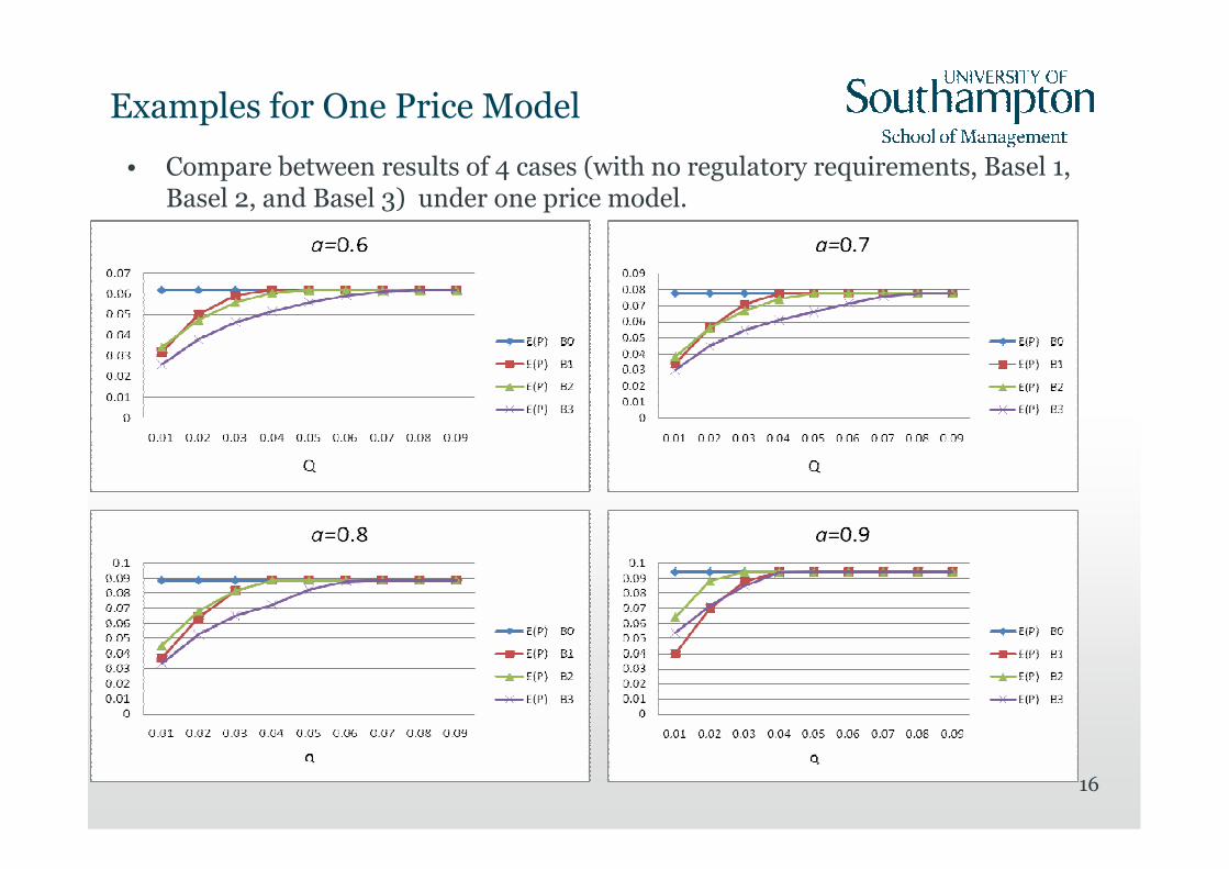
• Examples for one price model
� Optimal interest rates for Basel 1 , 2 and 3 are always bigger than that for Basel 0.
� The optimal interest rates charged drop but the expected portfolio profits rise up as the borrower portfolio become less risky.
� The expected portfolio profits for all Basel regulations are less than that of made with Basel 0.
� The expected portfolio profits under Basel 2 is smaller than that achieved under Basel 1 until one reaches the a=0.9 portfolio.
� The expected portfolio profits for Basel 3 is always smaller than that for Basel 1 and 2.
a r B0 E(p) B0 r B1 E(p)B1 r B2 E(p)B2 r B3 E(p) B3
� As a increases, the optimal cut off point and segment point increase and the expected portfolio profits increase as well
� As a increases, both interest rates decrease in order to be able to attract sufficient of the higher quality borrowers.
� Note that in all four portfolios we make offers to all the potential borrowers and make the offer of the better interest rate to just over half of them.
� There is a small increase in the optimal interest rates being charged by comparing with the solutions for Basel 0, while the profits are slightly lower.
� Again there an offer is made to everyone in the portfolio.
10
a EP B0
0.6 0.485568 0.6 0.317348 0.790765 0.07506936
0.7 0.415754 0.7 0.297977 0.845737 0.08508152
0.8 0.353758 0.8 0.279661 0.898441 0.09168503
0.9 0.297323 0.9 0.262075 0.94968 0.09493876
a EP B1
0.6 0.488475 0.6 0.319604 0.790703 0.07305781
0.7 0.418356 0.7 0.300156 0.845704 0.08304529
0.8 0.356118 0.8 0.281772 0.898428 0.0896575
0.9 0.299488 0.9 0.264128 0.949676 0.09294516
2r 1rcp *p
2r cp 1r*p
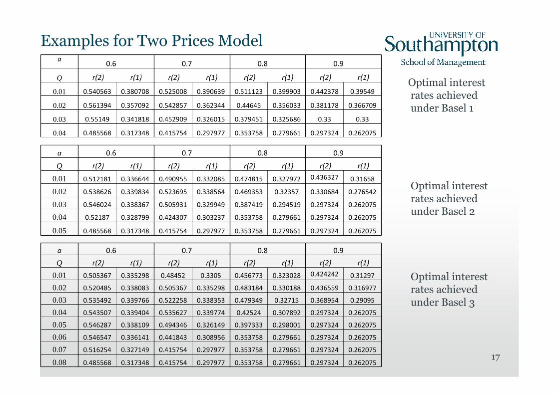
• Under Basel 2 (B2)
• Under Basel 3 (B3)
� The rate r1 under Basel 2 is always smaller than that for Basel 1, r2 is higher than that for Basel 1 if a=0.6 or 0.7 but lower than it if a=0.8 or 0.9.
� The expected profit is lower under Basel 2 than Basel 1 except in the case when a=0.9 where the potential set of borrowers is the least risky of the four cases.
� The expected portfolio profits for Basel 3 is always smaller than that for Basel 1 and 2.
� the rate r2 under Basel 3 only drops below the Basel 1 rate with the least risky portfolio a=0.9. The rate r1 is higher than the Basel 1 case if a=0.6 but then drops below the Basel 1 rate for “better”portfolios. 11
a EP B2
0.60.488913
0.6 0.31957 0.791461 0.072208
0.70.418609
0.7 0.299716 0.846327 0.082389
0.80.355927
0.8 0.280833 0.899 0.089405
0.90.298533
0.9 0.262549 0.950295 0.093397
a EP B3
0.6 0.491035 0.6 0.320974 0.79186 0.070447
0.7 0.420426 0.7 0.30082 0.846656 0.080727
0.8 0.357323 0.8 0.281591 0.899298 0.087995
0.9 0.299371 0.9 0.262907 0.950565 0.092441
2r
2r
cp
cp
1r
1r
*p
*p
Examples for variable pricing model
p r B0 r B1 r B2 r B30.35 1.015714 1.021429 1.022753923 1.027153
0.4 0.897501 0.902501 0.904159744 0.908321
0.5 0.72 0.724 0.725897785 0.729584
0.6 0.588333 0.591667 0.59344082 0.596632
0.7 0.482858 0.485714 0.487108924 0.489765
0.8 0.393751 0.39625 0.397027862 0.399076
0.9 0.315556 0.317778 0.317627495 0.318922
0.95 0.279474 0.281579 0.28075476 0.281555
0.96 0.272458 0.274542 0.27355002 0.274233
0.97 0.265506 0.267567 0.266391431 0.266945
0.98 0.258612 0.260654 0.259268093 0.259678
0.99 0.251778 0.253798 0.252164403 0.252406
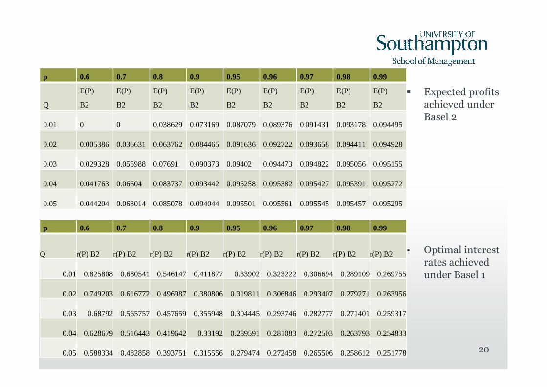
• Optimal interest rates under variable pricing
� The optimal interest rates charged decrease as p increases under all Basel regulation rules.
� The optimal interest rates for B0 are always less than those that for Basel 1, 2 and 3.
� The interest rates for Basel 2 are higher than that for Basel 1 until the probability of the borrowers being good is over 0.9.
� The optimal interest rates for Basel 3 also become smaller than that for Basel 1 as p is high enough.
12
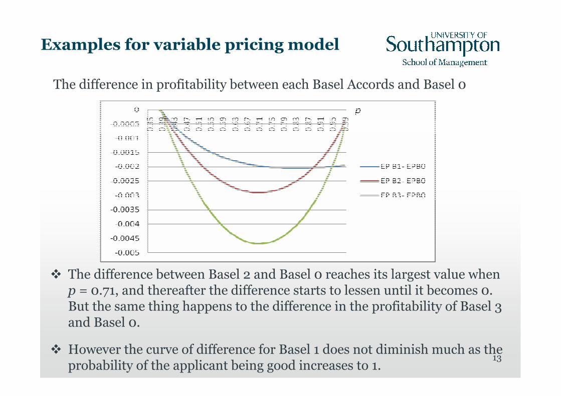
Examples for variable pricing model
The difference in profitability between each Basel Accords and Basel 0
� The difference between Basel 2 and Basel 0 reaches its largest value when p = 0.71, and thereafter the difference starts to lessen until it becomes 0. But the same thing happens to the difference in the profitability of Basel 3 and Basel 0.
� However the curve of difference for Basel 1 does not diminish much as the probability of the applicant being good increases to 1.
13
Price Models at Portfolio Level with Fixed Amount of Equity Capital
• Fixed (one) price model
subject to
• Two prices model
subject to
• Variable pricing model
subject to
Qdpprqpfpklcpa
D ≤⋅⋅⋅⋅∫1
),max(
),()()(
( )( ) ( ) ( )[ ]
( ) ( ) ( )[ ]
⋅⋅+−⋅+⋅+
⋅⋅+−⋅+⋅
=
∫
∫
dppfrlplrprq
dppfrlplrprq
prEP
p
FDD
p
pa
FDD
pprr
c
c
Max)(,
)(,
,1
11
),max(
22
,,,
*
*
*21
( ) ( ) ( ) ( )[ ] dppfrlplprprqaprEPa
FDDpr
Max ⋅⋅+−⋅+⋅= ∫ )()(,),(1
)(
14
( ) ( ) ( ) ( )[ ] dppfrlplrprqprEPcc pa
FDDpr
Max ⋅⋅+−⋅+⋅= ∫ )(,,1
),max(,1
Qdpprqpfpkldpprqpfpklp
D
p
pa
D
c
≤⋅⋅⋅⋅+⋅⋅⋅⋅ ∫∫1
1
),max(
2*
*
),()()(),()()(
Qdpprqpfpkla
D ≤⋅⋅⋅⋅∫1
),()()(
Examples for One Price Model
a 0.6 0.7 0.8 0.9
Qr r r r
0.01 0.401949 0.407457 0.414136 0.43
0.02 0.386739 0.393195 0.401949 0.380001
0.03 0.37903 0.384206 0.37 0.330001
0.04 0.376854 0.36 0.32 0.279998
15
The optimal interest rate to charge drops as the equity available increases under Basel 1 regulation.
Under the Basel 2 and Basel 3 the optimal interest rate increases as the equity available increases when there is very little equity available and then decrease as the equity increases when there is more equity available.
This is because increasing the interest rate has two counterbalancing effects.
a 0.6 0.7 0.8 0.9
Q r r r r
0.01 0.366959 0.362857 0.354892 0.349461
0.02 0.376899 0.374217 0.367484 0.356492
0.03 0.379852 0.378328 0.373242 0.340678
0.04 0.380205 0.37979 0.375172 0.292207
0.05 0.379504 0.380211 0.36719 0.292207
0.06 0.378389 0.380007 0.332626 0.292207
0.07 0.37736 0.379273 0.332626 0.292207
0.08 0.37686 0.355765 0.332626 0.292207
• Optimal interest rates achieved under Basel 1
• Optimal interest rates achieved under Basel 2
• Optimal interest rates achieved under Basel 2
a0.6 0.7 0.8 0.9
Q r r r r
0.01 0.374611 0.369972 0.363238 0.353655
0.02 0.38006 0.378746 0.374369 0.329441
0.03 0.37953 0.380226 0.370705 0.329441
0.04 0.377708 0.379595 0.315316 0.329441
0.05 0.377513 0.351949 0.315316 0.329441
Examples for One Price Model
• Compare between results of 4 cases (with no regulatory requirements, Basel 1, Basel 2, and Basel 3) under one price model.
Conclusions• Using variable pricing the resultant profit is always the highest of the three, and profit achieved by using two prices model is always higher than that of using one price model.
• The profit made with B0 is always the greatest among the four cases if there is no any impact of adverse selection. If the borrower has a good quality, then B2 will give more profit to the lender than B1. And if the borrower is more risky, then the lender make more profit with B1. The expected portfolio profits for Basel 3 is always smaller than that for Basel 1 and 2.
• For predetermined equity capital, if the lender only has a little equity then the lender can make more profit with B2 than B1, but if the lender has more equity then they are taking more of the risky applicants and so B1 gives more profit than B2. With higher quality borrowers, the expected profit for Basel 3 lies between the Basel 1 and Basel 2 if the capital restriction of Q is very small.


![Bo-Chih Huang x{ November 17, 2015 …math.ncu.edu.tw.:Department of Mathematics, National Central University, Chung-Li 32001, Taiwan, E-mail: ... arXiv:1511.00804v2 [math.AP] 16 Nov](https://static.documents.pub/doc/80x56/5ace2e6d7f8b9a6c6c8b83cc/bo-chih-huang-x-november-17-2015-mathncuedutwdepartment-of-mathematics.jpg)


