Human Capital and Economic Opportunity: A Global Working Group

Working Paper Series

Human Capital and Economic Opportunity Working GroupEconomic Research CenterUniversity of Chicago1126 E. 59th StreetChicago IL 60637humcap@uchicago.edu

Working Paper No.

Group Decision Making with Uncertain Outcomes:

Unpacking Child-Parent Choices of High School Tracks∗

Pamela Giustinelli†

University of Michigan

July 15, 2011

Abstract

Predicting group decisions with uncertain outcomes involves the empirically difficult task of disentan-

gling individual decision makers’ beliefs and preferences over outcomes’ states from the group’s decision

rule. This paper addresses the problem within the context of a consequential family decision concerning

the high school track of adolescent children in presence of curricular stratification. The paper combines

novel data on children’s and parents’ probabilistic beliefs, their stated choice preferences, and families’

decision rules with standard data on actual choices to estimate a simple model of curriculum choice

featuring both uncertainty and heterogeneous cooperative-type decisions. The model’s estimates are

used to quantify the impact on curriculum enrollment of policies affecting family members’ expectations

via “awareness” campaigns, publication of education statistics, and changes in curricular specialization

and standards. The latter exercise reveals that identity of policy recipients–whether children, parents,

or both–matters for enrollment response, and underlines the importance of incorporating information

on decision makers’ beliefs and decision rules when evaluating policies.

[JEL codes: C25, C35, C50, C71, C81, C83, D19, D81, D84, I29, J24.]

[Key words: Choice under Uncertainty, Multilateral Choice, Heterogeneous Decision Rules, Curricular

Tracking, Curriculum Choice, Child-Parent Decision Making, Subjective Probabilities, Stated and Revealed

Preferences, Choice-Based Sampling.]

∗This paper is based on the second chapter of my Ph.D. dissertation. An earlier version was circulated as my job marketpaper under the title “Understanding Choice of High School Curriculum: Subjective Expectations and Child-Parent Inter-actions.” Acknowledgements: I heartily thank Chuck Manski for his helpful comments on this work and for his constantencouragement and guidance throughout dissertation, as well as the other members of my dissertation committee, DavidFiglio, Joel Mokyr, and Elie Tamer, for their availability and feedback. I am enormously indebted to Paola Dongili and DiegoLubian for without their support and friendship this project would have not come into existence. I have greatly benefited frompatient and insightful discussions with Federico Grigis and from precious inputs on different issues and at different stages byPeter Arcidiacono, Ivan Canay, Matias Cattaneo, Damon Clark, Adeline Delavande, Jon Gemus, Aldo Heffner, Joel Horowitz,Diego Lubian, Peter McHenry, Aviv Nevo, Matthew Shapiro, Zahra Siddique, Chris Taber, Basit Zafar, Claudio Zoli, andseminar participants at the 2009 MOOD doctoral workshop (Collegio Carlo Alberto, Turin, Italy), Northwestern U., the VIIIBrucchi Luchino workshop (Bank of Italy, Rome, Italy), U. of Verona, the V RES Ph.D. Meeting (City U., London, UK), U.of Michigan SRC, U. of Michigan Economics, U. of Maryland AREC, U. of East Anglia, Uppsala U., U. of Alicante, U. ofKonstanz, U. of Bern, the 2010 MEA Annual Meeting (Evanston, IL, USA), the 2010 EEA Summer Meeting (U. of Glasgow,Glasgow, UK), the Institute of Education (U. of London), and the 2011 AEA Annual Meeting (Denver, CO). Warm thanksalso to Stefano Rossi for useful suggestions and tireless support with the revision, and to Marco Cosconati for countless syn-ergic inputs originating from a joint related project. Data collection was funded by the SSIS of Veneto, Italy, whose financialsupport I gratefully acknowledge together with that of the University of Verona. All remaining errors are mine.†Correspondence to: Pamela Giustinelli, University of Michigan, Survey Research Center, 1355 ISR Building, 426

Thompson Street, Ann Arbor, MI 48106 U.S.A. Office phone: +1 734 764 6232. E-mail: <pgiusti@isr.umich.edu>

“If one studies humanities in a general high school, but after 5 years he no longer wishes to go touniversity, what can he do? And after studying art in a general high school? Because when one is 14 hemakes a choice, and thinks that, perhaps, he will go to college afterwards... But after 5 years he mightchange his mind. And if he is fed up with school, then he can go to work [if he attended a technical orvocational school, instead].” (a brother) (Istituto IARD, 2001, p.62)1

“As for the high school curriculum, she decided what to study. She chose the school, but only after wehad talked together. Her father, for instance, preferred another [type of] school and, perhaps, I hopedfor yet a different one. But she made her own choice in the end, after a series of discussions we hadtogether.” (a mother) (Istituto IARD, 2001, p.39)

1 Introduction

Social researchers and policy makers have long been interested in analyzing and predicting

choices with uncertain outcomes and multiple decision makers. These choices span human cap-

ital investment, sexual behavior, crime behavior, and countless others. For instance, members

of criminal gangs choose whether to commit crimes with partial knowledge of their probability

of being arrested; sexually active partners make contraceptive choices with partial knowledge

of effectiveness and side effects; family members select curricular tracks for their children with

partial knowledge of children’s tastes, ability, and future opportunities and choices. However,

predicting any of these behaviors to inform policy requires disentangling decision makers’ be-

liefs and preferences over outcomes’ states from the group’s decision rule. This is because there

will generally exist several configurations of beliefs, preferences, and decision rules that are

compatible with the same observed choice and have different implications for policy.

In this paper, I focus on choice of high school curriculum with curricular tracking, and

I address the identification problem of empirically distinguishing how children’s and parents’

beliefs and preferences over choice-related outcomes drive curriculum choice via heterogeneous

rules of child-parent decision making. Nonetheless, while substantively my analysis is relevant

both for the debate on intergenerational transmission of beliefs and preferences from parents to

children (e.g., Bisin and Verdier (2001) and Doepke and Zilibotti (2008)) and for understanding

the role of preferences and information in career-oriented school choices (e.g., Arcidiacono et al.

(2011) and Zafar (2008))–and hence for educational policy–the framework I study is more

general. It encompasses any choice situation featuring a small group of decision makers that

face a common discrete choice with uncertain outcomes, hold subjective beliefs and individual

preferences over outcomes’ states, and employ a cooperative-type decision rule aggregating their

preferences and beliefs and nesting more unilateral decisions as special cases.2

1From the Istituto IARD (2001)’s sociological study. My translation from Italian.2From a theoretical perspective, the paper’s setup may be thought of as an application of Savage (1954)’s framework and

Harsanyi (1955)’s utilitarian aggregation combined, as recently conceptualized and discussed by Gilboa et al. (2004). Animportant feature of this framework is that unanimity of group members’ preferences over alternatives does not imply thatan individually preferred alternative is also socially preferred, since unanimity may be generated by different combinations ofindividual preferences and beliefs over states of nature (see Mongin (2005)’s in-depth discussion and Raiffa (1968)’s “Paretians-vs.-Bayesians” dramatization). In fact, while I assume that decision makers are individually rational–in the sense that theymaximize expected utility–I do not assume a priori that they hold rational expectations nor I make any specific assumptionabout the manner in which they update their own beliefs based on information they receive from the other members of the

1

To illustrate, let us consider the choice faced by an adolescent child (“he”) and his parent

(“she”), both wishing to select the best curriculum for the child between art and math. For

simplicity, let child and parent be only concerned with the child’s taste for subjects and the

program’s difficulty level given child’s ability, all of which are uncertain. Child and parent hold

subjective probabilistic beliefs over realization of different taste and difficulty states and attach

individual valuations to them. (Perhaps the child thinks he is an artist and should follow his

talent, whereas his mother thinks he has got what it takes to become a brilliant mathematician!)

Moreover, either the child makes curriculum choice individually or child and parent make a joint

decision.

In this setting, being able to tell beliefs and preferences apart is important for policy makers,

since expectation-driven choices may be affected by some policy, e.g., by provision of informa-

tion about subjects and difficulty levels, while preference-driven choices may require a different

policy, e.g., no policy. Furthermore, identifying the target–child, parent, or both?–of a policy

that aims at affecting curriculum enrollment via information provision and assessing the poten-

tial effectiveness of such a policy via counterfactual analysis require uncovering the role played

by each decision participant in the choice.

Thus far, insufficient prior knowledge and lack of adequate data on how individuals and

groups make decisions with uncertain outcomes has rendered this identification problem hard

to tackle empirically (Manski, 2004a, 2000). First, commonly available data are limited to

decision makers’ characteristics and some features of the alternatives. Second, any statistical

analysis associating choices with decision makers’ background characteristics usefully reveals

“which individuals or groups choose what” but does not uncover the main decision-making

channels nor can be used to answer counterfactual policy questions. Last but not least, while

counterfactual analysis relies on structural modeling, identification and estimation of structural

models from standard data requires strong non-testable assumptions.

My work addresses these issues directly by collecting new data on usually unobserved prim-

itives of a family decision process and by showing how such data can be used in the estimation

of a simple model of curriculum choice with uncertain outcomes and heterogeneous child-parent

decision-makings to achieve identification and make inference on families’ choices. The paper

thus tackles some of the aims of existing research agendas on behavioral choice modeling (e.g.,

Ben-Akiva et al. (2002) and Adamowicz et al. (2008)), especially concerning decision making

under uncertainty (e.g., Manski (2004a, 2000)) and within the family (e.g., Dauphin et al.

(2010)).

In particular, I designed and conducted a survey gathering the following field data from a

relatively large sample of Italian families:

(A) Children’s and parents’ probabilistic expectations before the choice, elicited on a 0-100

group. On the other hand, analysis of identification depends on the adopted framework.

2

scale, over several in-high-school and post-diploma outcomes;

(B) Children’s and parents’ stated choice preferences before the choice (SP);

(C) Families’ actual choices, or revealed preferences (RP);

(D) Self-reported family decision rules, including (1) unilateral decision by child (parents),

(2) choice by child (parents) after listening to the parents (child), and (3) child-parents

joint decision;3

(E) Orientation suggestions provided by junior high school teachers;

(F) Children’s and families’ background characteristics.

Then, within the theoretical framework previously outlined, I demonstrate how joint use of these

data can be employed to separately identify and estimate structural parameters capturing how

children and parents trade off different choice-relevant outcomes (preference or utility weights)

and parameters describing family decision rules (aggregation or protocol weights).4

Specifically, with actual choices (C) observed, identification of the empirical model works

as follows. Under unilateral decisions (and under “unitary family” decision in the sense of

Becker (1981)), heterogeneity in decision makers’ probabilistic expectations (A) identifies utility

parameters, in the same fashion as alternatives- and decision makers-specific characteristics do

in standard random utility models with no uncertainty. Actual choices (C) and family members’

expectations (A), however, do not suffice to separately identify preference and aggregation

parameters for families making a multilateral decision according to (D). To solve this problem,

I combine data (A) and (C) with family members’ stated preferred alternatives (B), within

a stated preference-revealed preference (SP-RP) joint framework (e.g., Ben-Akiva et al. (1994)

and Hensher et al. (1999)). Intuitively, given data on family members’ choice preferences,

utility weights are identified from heterogeneity in expectations (one SP individual choice model

for each family member with an “active” decision-making role); whereas, protocol weights are

identified from differences between family members’ individual choice preferences and families’

actual choices (one RP family model of multilateral decision making).

Thus, methodologically, my paper bridges an emerging literature in economics with a liter-

ature that has long developed mainly outside economics, in the fields of transportation, mar-

keting, and resource economics. The former is a stream of works employing “right-hand side”

probabilistic expectations data in models of individual choice under uncertainty to achieve or

improve identification of structural preference parameters (e.g., Delavande (2008), Arcidiacono3Rule (1) holds that the child chooses by maximizing his subjective expected utility formed by his own preferences and

beliefs over outcomes’ states. Rule (2) holds that the child chooses by maximizing a subjective expected utility formed by hisown preferences over outcomes’ states and by beliefs updated to account for parental beliefs. Rule (3) holds that child’s andparent’s preferences and beliefs over outcomes’ states contribute to the final choice via linear aggregation of the correspondingexpected utility components. A formal representation is provided in subsection 2.3.

4Notice that I can focus on curriculum demand because the Italian secondary system features open enrollment. That is,lack of selectivity from the school side eliminates potential identification problems from the interplay of demand and supplyin producing observed choices.

3

et al. (2011), and Zafar (2008) for static choices, and Erdem et al. (2005) and Mahajan and

Tarozzi (2011) for dynamic settings).5 The latter, originating from Morikawa (1989)’s original

work, suggests pooling SP and RP data together–a process called “data enrichment” or “data

fusion”–in order to exploit SP data to help identify parameters that RP data could not and,

thus, improve estimation efficiency (see Louviere et al. (2000)’s state-of-the-art review). Both

streams of literature, however, have focused on unilateral decision making and, to the best of

my knowledge, the latter has never been used for analyzing group decisions with uncertain

outcomes.6

The empirical tool developed in this paper enables me to investigate the following descriptive

and normative issues of curriculum choice:

(I) What are the most important determinants of curriculum choice among future outcomes–

defined over children’s “taste” for curricula, their ability and effort while in high school, and

post-graduation opportunities and choices–that are uncertain at the moment of curriculum

choice and are potentially relevant for it?

(II) Conditional on an interacted family decision rule, to what extent are parental beliefs

transmitted to children during the decision, and to what extent do parental preferences

affect the final choice?

(III) How does curriculum enrollment respond to policy-induced changes of decision makers’

beliefs over outcomes’ states? And is it important to account for child-parent decision

making and heterogeneous family rules for counterfactual analysis of curriculum choice?

I find that preference or taste for curriculum core subjects is systematically the most valued

factor by both children and parents and across families using different decision rules. Whereas

the importance of other in-high-school outcomes relative to post-diploma ones (e.g., school

achievement and effort relative to flexible college-work and college major choices) is heteroge-

neous across groups (issue I).

Estimates of the model with heterogeneous decision rules reveal that children incorporate

parents’ beliefs into their own when making the choice at least partially and to an extent that

varies across outcomes (issue II, family rule 2). For instance, children appear to trust

parental opinion regarding their ability better than their own, assigning a larger weight to the

former. On the other hand, the aggregation weights on the flexibility that different curricula

will provide in the subsequent choice of field in college and the aggregation weights on child’s

preference for subjects favor children’s opinions, although equal weights cannot be rejected for

the latter outcome.5Other recent papers have used expectations data as equilibrium outcomes in discrete choice with social interactions (Li and

Lee, 2009) and, on the “left-hand side,” as a response variable for choice experiments under incomplete scenarios (Blass et al.,2010), to improve estimation efficiency (e.g., van der Klaauw (2000)), and to identify unobserved heterogeneity in dynamicsettings (Pantano and Zheng, 2010).

6Dosman and Adamowicz (2006) are a partial exception in that they use SP-RP methods to examine household vacationsite choice with inter-spouses bargaining, but their setting does not feature uncertainty nor heterogeneous decision processes.

4

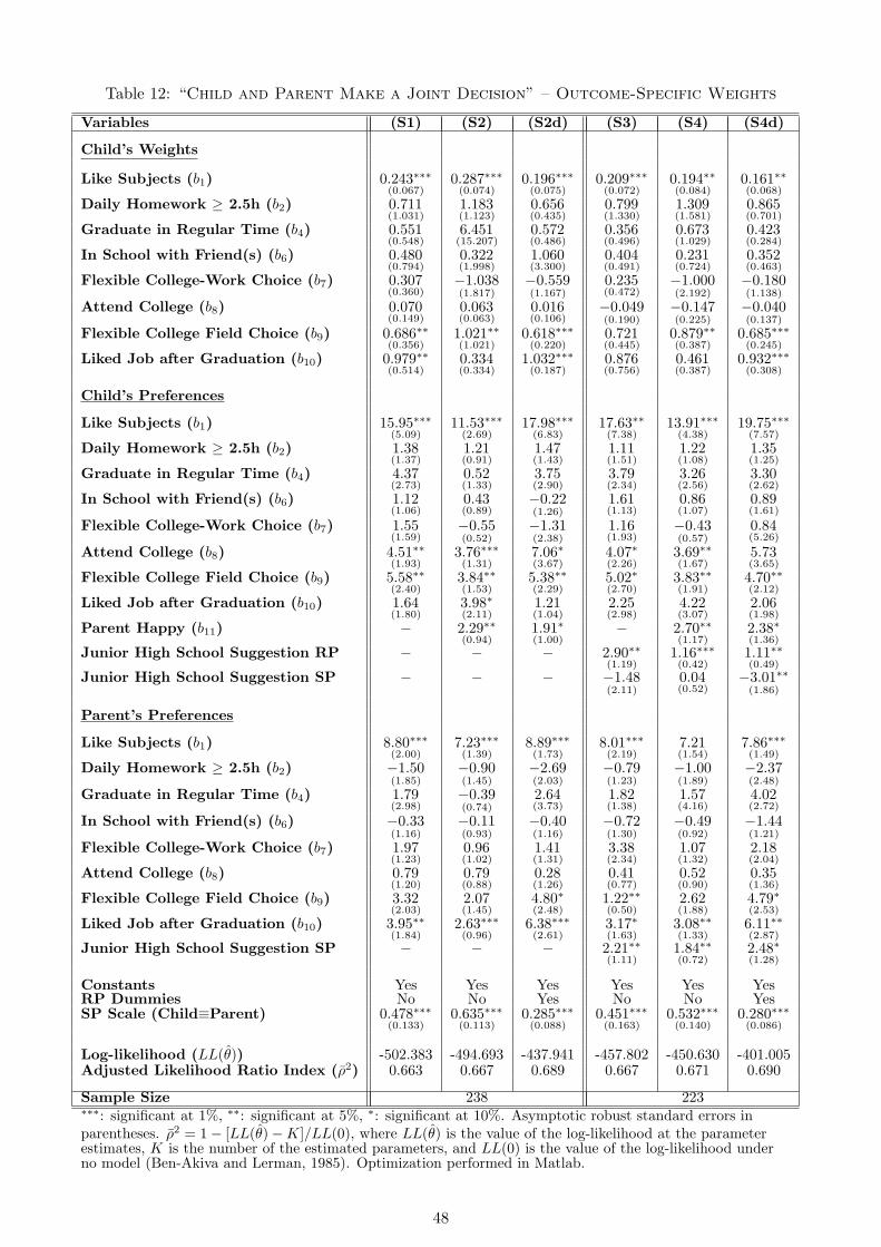
Comparison of children’s and parents’ stated choice preferences with actual choices for fami-

lies in which child and parent(s) make a joint decision supports group rationality, with less than

5% of families selecting an individually dominated choice. Moreover, parameters’ estimates for

this group suggest a substantial influence of parental preferences on curriculum choice (issue

II, family rule 3). For instance, the weight on the child’s expected utility component of taste

for subjects is smaller than 1/3, and a weight of 1/2 is statistically rejected. That is, parents

may be trying to prevent children from overweighting their own preferences for subjects in high

school relative to other outcomes that will realize at a later time in their future. On the other

hand, the aggregation weights on the flexibility that different curricula will provide when chil-

dren face the college field choice and those concerning the possibility of finding a liked job after

graduation favor children’s preferences. Nonetheless, weights’ heterogeneity across outcomes is

not statistically significant, and a unique weight of approximately 1/3 on the child’s expected

utility cannot be rejected.

I use the models’ estimates to simulate counterfactual scenarios in which changes in indi-

viduals’ beliefs–generated by “awareness” campaigns, publication of education statistics, and

policies altering curricular specialization and standards–affect curriculum enrollment (issue

III). For instance, simulation of a 0.1 increase in individuals’ probabilities of enjoying math

and science in the general scientific curriculum following an awareness campaign about those

subjects shows that the large utility weight families attach to the child’s taste for subjects im-

plies a potentially large impact of this kind of policies on curriculum enrollment. Altering access

to university based on children’s graduation curriculum has also a large impact on response,

as opposed to providing information on curriculum graduation rates and on subsequent college

enrollment for previous cohorts.

As for heterogeneity of family decision rules, the unitary-family benchmark and the proposed

model with heterogeneous rules generate intuitive and qualitatively similar predictions that,

nonetheless, are quantitatively different. In particular, the counterfactual exercises reveal that

identity of policy recipients matters for enrollment response and underlines the importance of

incorporating decision makers’ beliefs and decision rules when evaluating policies. For instance,

assuming a unitary model with parents as representative decision makers sizeably overestimates

the magnitude of enrollment response to awareness and desensitization campaigns implied by the

heterogenous model; whereas a unitary model based on children’s expectations generates much

closer predictions. Moreover, counterfactual enrollment responses decomposed by decision-

making rule and by targeted group suggest that publication of education statistics would have

a larger impact on children reporting unilateral decision by self than on the other children,

and that if parents only were aware of policies changing institutional features of tracking, the

impact of such policies may be much smaller than if children, too, were informed.

While direct observation of family members’ probabilistic beliefs and decision rules makes

5

modeling expectations and assuming a particular decision-making unit unnecessary–a main

strength of my analysis–it should be clear nonetheless that the approach I explore with this

work does not mean to nor can eliminate the need of assumptions altogether. Rather, it

transfers their locus from things researchers do not know to be true nor can usually test, i.e.,

the behavioral process, to elements over which they may have some control or at least better

information, i.e., the collection and properties of the data. Thus, for example, I take data

on expectations and family decision rules at face value. Trusting the reader’s patience and

hoping to achieve greater transparency, however, I defer a more thorough discussion of these

and related aspects, including potential limitations, to the body of the paper–where they can

be more conveniently related to the formal setup–and to the concluding session–where I briefly

summarize them and identify areas of future work.

The paper is organized as follows. Section 2 conceptualizes child, parent, and family choice

problems, and illustrates the main identification and policy issues through a simplified example

with two decision rules, two alternatives, and two binary outcomes. Section 3 covers the study

design and describes the samples used in the empirical analysis of section 4. Section 5 presents

the counterfactual policy exercises. Section 6 relates the paper to the literature. Conclusions

follow.

2 The Identification Problem, Idealized

2.1 Curriculum Choice under Uncertainty

Setup. The environment is populated with families, f = 1, ..., F ∈ F , each one formed by

one adolescent child, c = c(f), and one parent, p = p(f). Families face high school curriculum

choice for their children over a common set of available alternatives, j = 1, ..., J ∈ J , and wish

to make an optimal child-curriculum match as follows:

maxj∈J

θcj , (1)

where θcj is the quality of the match between child c and curriculum j. This parameter should

be thought of as multidimensional, encompassing both quality of curriculum choice during high

school and opportunities and choices after graduation. Examples are whether the child would

enjoy the core subjects, how his academic performance would be, and which opportunities and

choices would he face after graduation, should he enroll in curriculum j.

Families are likely to perceive most if not all components of θcj as uncertain at the mo-

ment of the choice. Assuming separability of θcj ’s components yields a convenient repre-

sentation of uncertainty as a set of binary outcomes, B = {bn ∈ {0, 1}}Nn=1, with corre-

sponding objective ex-ante realization probabilities, {Πcj (bn ∈ {0, 1})}n=1,...,N ;j=1,...,J , such that

6

Πcj (bn = 1) = 1 − Πcj (bn = 0). Hence θcj can be expressed as a function of such probabili-

ties, i.e., θcj = θ({Πcjn}Nn=1

), with j = 1, ..., J . In fact, I assume that family members hold

subjective probabilistic beliefs, {Pij (bn ∈ {0, 1})}n=1,...,N ;j=1,...,J with i ∈ {c, p}, which may or

may not coincide with the objective ones and based on which they form estimates of θcj , i.e.,

θij = θ({Pijn}Nn=1

). Hence, to clarify, Πcjn = Πcj (bn = 1) indicates the objective ex-ante prob-

ability that outcome bn = 1 occurs if child c attends curriculum j; whereas, Pijn = Pij (bn = 1)

indicates the subjective probability held by family member i ∈ {c, p} for the same outcome.

Finally, in my notation, individuals’ indices indicate individual-specific variables or param-

eters, when used as subscripts; they indicate variables or parameters specific to the class of

individuals identified by the index, when used as superscripts.

Assumptions. Before moving to the example, I wish to make the assumptions underlying

the described framework more transparent and to provide motivations for them. Whenever

warranted, I will defer further discussions to later sections.

First, I assume dyadic families because data on beliefs and stated choice preferences were

collected for one parent only. Theoretically, this is equivalent to assuming that parental role

in the choice can be represented through primitives of a single parent, the “representative”

or “relevant” parent. Inclusion of both parents into the framework would be conceptually

straightforward, as it will become clear in subsections 2.3 and 4.2.

Second, based on the institutional features relevant for the empirical analysis, the supply

side is characterized (1) by curricular tracking with physically separate curricula (i.e., offered

by different schools) and (2) by an open enrollment system in which the allocation mechanism

of children to curricula and schools is family choice.7 On the demand side, I assume (3) a

hierarchical process of (a) selection of a family decision rule, (b) curriculum choice, and (c)

school choice, as well as (4) separability of curriculum choice from other family choices. (1)

and (2) allow me to focus on the demand side; (3) and (4) allow me to analyze curriculum

choice in isolation. While I discuss separability of family decision rule and curriculum choice

later in the paper, separability of curriculum choice from school choice is supported by the fairly

homogeneous quality of Italian public schools, to which I restrict in the empirical analysis.

Third, I assume that all families face the same “universal set” of alternatives and that they

use it as their choice set for curriculum choice. The former assumption is warranted for my

empirical analysis, since the size of the area where the data were collected, the schools’ location

within the area, and the characteristics of the public transport network make all curricula

available to everybody (see Giustinelli (2010, Chpt. 2) for details). On the other hand, the latter

assumption–commonly made in empirical applications–excludes the possibility of heterogeneous

non-compensatory processes of “consideration set” formation. Later I will identify this aspect7See section 6 for a short summary about curricular stratification in Italy and other OECD countries or Giustinelli (2010,

Chpt. 2) for a more detailed one.

7

as an interesting candidate for further work, as it constitutes an additional channel through

which parents and teachers may affect children’s curriculum choice.

Finally, choice of modeling uncertainty as a set of separable binary outcomes is purely dic-

tated by feasibility of data collection so that, for each respondent i ∈ {c, p}, {Pij (bn = 1)}n=1,...,N ;j=1,...,J

are elicited in place of the more complicated objects {Pij (b1, ..., bN )}j=1,...,J . Notice also that

if multiple discrete or continuous outcomes were included, multiple points of the respondents’

distributions of beliefs should be elicited for each outcome and alternative.

A 2×2×2 Example. Throughout the section, I illustrate the framework and the identi-

fication problem via a simple example with 2 alternatives, 2 outcomes, 2 family decision

rules or “protocols,” and 1 family. The family must choose between the art curriculum,

“Michelangelo” (M), and the math-and-science curriculum, “Galileo” (G), by weighing a “Dif-

ficulty” outcome (D)–that the child will graduate from high school in the regular time–and

a “Flexibility” outcome (F)–that the training he receives in high school will allow him to

choose among a wide range of fields in college. An M-diploma would be easier to obtain

for this child than a G-diploma: ΠcMD = 95 > ΠcGD = 70 (math at Galileo is really

hard!). However, an M-diploma would provide him with less flexibility than a G-diploma:

ΠcMF = 30 < ΠcGF = 90 (Michelangelo’s artistic training is somewhat narrow and suit-

able only for studying architecture or some art-related field in college). Family members

hold subjective assessments, {(PiMD, PiMF ); (PiGD, PiGF )}i∈{c,p}, of the objective probabili-

ties, {(ΠMD,ΠMF ); (ΠGD,ΠGF )} = {(95, 30); (70, 90)}, and use the former within one of the

following decision processes: either the child unilaterally chooses his own curriculum or child

and parent make a joint decision.

2.2 The Individual Problem: Separating Preferences and Beliefs

Analysis of the individual curriculum choice problem–as faced by a single family member o by

a unitary decision-making unit–introduces the challenge of empirically separating the decision

maker’s preferences from his/her beliefs.

The Child Problem. Faced with the curriculum choice problem, the child selects the cur-

riculum that maximizes θcj over J , according to decision rule (1). I operationalize this idea

by assuming that he maximizes the following linear, separable-in-outcomes, and subjective

expected utility:

EUcj =N∑

n=1

∑bn∈{0,1}

Pcj (bn) · u(bn, zc) + x′cjδ(zc) + εcj =N∑

n=1

Pcjn ·∆ucn + U c + x′cjδ

c + εcj , (2)

8

which is a function of the vector of uncertain outcomes, b = (b1, ..., bN ), of a M × 1 vector of

child-curriculum specific attributes not subject to uncertainty, xcj = (xcj1, ..., xcjM )′, of a vector

of individual characteristics, zc, and of a random term unobservable to the econometrician, εcj .

Being constant over alternatives, U c =∑N

n=1 u(bn = 0, zc) drops out of the choice.

Each structural preference parameter, ∆ucn = u(bn = 1, zc) − u(bn = 0, zc), represents the

difference in utility that a child with characteristics zc derives from occurrence of outcome n

(i.e., bn = 1), relative to its non-occurrence (i.e., bn = 0). Hence, these parameters combine

within a simple compensatory framework the different components of θcj , and should not be

confused with the child’s “choice preference” (i.e., his preferred alternative as implied by his

underlying utility) nor with his “preference or taste for subjects” (i.e., a specific component

of his utility function). In particular, while the child may not perfectly know his taste for

subjects beforehand–indeed he holds subjective beliefs about it–the compensatory rule he uses

to trade off different outcomes reflects his preferences over outcomes’ states at the moment of

the choice.8

Linearity of expected utility implies risk-neutrality. However, sociological evidence suggests

that some children prefer curricula that–they believe–will enable them to “insure” against the

presently uncertain outcomes of their future college and work choices, i.e., to “postpone” those

choices.9 Indeed, economic theory has shown that risk aversion can generate preference for

flexibility both in presence and in absence of learning over time (Ficco and Karamychev, 2009).

To account for this aspect, albeit in a somewhat “reduced form” fashion, in the empirical model

I include children’s perception of the degree of flexibility that different curricula would give to

them in the future choices of college versus work and of college major.

Example (continued). Let us assume that the family is observed (by an econometrician) to

choose alternative M. Furthermore, let us momentarily assume that the family decision protocol,

e.g., unilateral decision by the child according to “ Maxj∈{M,G}

EUcj = PcjD ·∆ucD + PcjF ·∆ucF ,”

is also observed. Even within this simple setup, the researcher is faced with multiple competing

explanations consistent with choice of M. The following two scenarios illustrate the identification

problem and its relevance for policy.

• Scenario I: The child holds rational expectations, i.e., {(PcMD, PcMF ); (PcGD, PcGF )} =8Of course, preferences for outcomes realizing far ahead in time may differ from current preferences because of discounting

and/or time inconsistency. However, I do not incorporate these aspects in the model, since my data would not enable me toidentify the corresponding parameters. See Mahajan and Tarozzi (2011) for a recent paper using expectations data to identifytime preferences with heterogeneous time inconsistency.

9“I chose this school because beyond giving me this training [learning some foreign languages] ... afterwards I would liketo study law in college. But should anything happen to me, [with this diploma] I can still get a job in a travel agency... Noteverything is lost! It [this school] will provide me with several job opportunities.” (a girl attending a vocational school fortourism) (Istituto IARD, 2001, p.38) And her mother agrees “Perhaps, once A. has gotten her diploma she may change hermind, and decide she does not wish to go to college after all... Yet, [thanks to this training] she will hold a diploma that willenable her to find a job. A piece of paper is chased!” (Istituto IARD, 2001, p.38) On the other hand, a boy confident that hewill go to college comments “I knew I would go to college and I could do well in any type of general high school. Then, they[the parents] said ‘The scientific curriculum is better because you will have more options afterwards.’ That is, it is a schoolthat will enable me to choose among a large number of fields in college.”(Istituto IARD, 2001, p.39)

9

{(95, 30); (70, 90)}, and only cares about difficulty, e.g., {∆ucD,∆ucF } = {10, 0}. With a

linear compensatory rule trading off difficulty and flexibility, this configuration of prefer-

ences and beliefs implies EUcM = 95 · 10 + 30 · 0 > EUcG = 70 · 10 + 90 · 0.

• Scenario II: The child holds rational expectations on difficulty, but he erroneously per-

ceives the two alternatives as providing the same degree of flexibility, e.g., {(PcMD, PcMF );

(PcGD, PcGF )} = {(95, 90); (70, 90)}. Moreover, he equally cares about difficulty and flexi-

bility, e.g., {∆ucD,∆ucF } = {5, 5}. This yields EUcM = 95·5+90·5 > EUcG = 70·5+90·5.

Under the standard assumption that individual preferences (i.e., the utility weights) are

hardwired and cannot be manipulated, scenario I (a preference-driven choice) has different

policy implications than scenario II (an expectation-driven choice). Specifically, if a policy

maker were to intervene by providing the child with the correct information–optimistically

assuming that the policy maker knows it–his policy would be potentially effective only under

the second scenario. That is, if the now informed decision maker of scenario II were to

“comply” and used the disclosed objective realization probabilities, he would switch to choice

of G (since 95 · 5 + 30 · 5 < 70 · 5 + 90 · 5). Under scenario I, instead, the decision maker will

choose M even without holding rational expectations, as long as he does not value flexibility

and he correctly perceives M as an easier alternative.

The Parent Problem. I assume that parents put themselves in their children’s shoes–

meaning that they solve the same problem as their children do–but do it through their own

lenses–i.e., through their own subjective expectations and preference weights. This echoes Bisin

and Verdier (2001)’s assumption of parental “imperfect empathy,” and implies that the parental

problem can be formalized as in (2), substituting the individual index c with p.

2.3 Group Decision Making: Separating Members’ Preferences, Beliefs, and

Decision Rule

The Family Problem. A family-level decision process for curriculum choice may consist of

a unilateral decision by a single family member or may entail interactions among members.10

Specifying a particular form of interaction requires knowledge or assumptions on whether,

which, and how family members’ beliefs and preferences enter the process, and on whether and10Becker (1981, p. 298) reasons, “Of course children (in modern times, especially adolescents) may believe that they do

know enough and that their parents are out of touch with important changes (...) The conflict with older children is usuallyless severe, and altruistic parents are more willing simply to contribute dollars that children can spend as they wish (...)[This conflict] means that a common utility function for the family does not exist; different members maximize different utilityfunctions.” For instance, a girl of the Istituto IARD (2001)’s study narrates, “They never wished to influence me too much,I think because, should it turn out that the choice they imposed is a mistake, they would regret it! Hence, they let me free.”(Istituto IARD, 2001, p.63) While a mother says, “I liked such a clear idea, and I agreed!” (Istituto IARD, 2001, p. 59), withreference to the fact that her son provided a clear supporting argument for his choice. And yet, another girl explains, “Mymom wanted me to attend the artistic high school, and my father the accounting track. But I chose a school that will train meto become a teacher, instead. Thus, I gave them both the sack.” (Istituto IARD, 2001, p. 61)

10

how the choice set and other constraints are modified by the interaction itself.11

Set the latter issue aside, a fairly general formalization of a cooperative decision process

under uncertainty, nesting unilateral decision and other collective processes as special cases,

incorporates both revision of decision makers’ expectations and negotiation over preferences as

follows:

Maxj∈J

Γkfj =

N∑n=1

φcn ·{[wc,k

n · Pcjn + (1− wc,kn ) · Ppjn

]·∆uc,k

n

}+

+ (1− φcn) ·

{[(1− wp,k

n ) · Pcjn + wp,kn · Ppjn

]·∆up,k

n

}+

+M∑m

ϕcm ·[δc,k · xcjm

]+ (1− ϕc

m) ·[δp,k · xpjm

]+ εkfj . (3)

Hence, child and parent update their subjective beliefs, {{{Pijn}Nn=1}Jj=1}i∈{c,p}, to account for

each other’s opinions and information using outcome-specific weights, {wc,kn }Nn=1 and {wp,k

n }Nn=1

respectively. And they maximize a weighted average of their thus updated subjective expected

utilities, using a different set of outcome-level weights, {φcn}Nn=1 and {ϕc

m}Mm=1, that reflect

how much “outcome-specific say” each member has in the choice. {∆uin}Nn=1 and {δi

m}Mm=1

denotes family members’ preference over outcomes (dependence of the preference parameters on

individual characteristics is suppressed for notational convenience), and {εkfj}Mm=1 is a random

component capturing the observational difficulty of the econometrician.

Example (continued). For the sake of the example let us now assume that whenever child

and parent make a collective decision, they solve

maxj∈{M,G}

φc · [PcjD ·∆ucD + PcjF ·∆ucF ] + φp · [PpjD ·∆upD + PpjF ·∆upF ] .

This process is nested in problem (3), with {wc,kn , wp,k

n } ≡ {1, 1}, φcn ≡ φc ∀n, and φp = 1− φc.

It is then easy to concoct a third scenario in which, choosing according to this rule, child and

parent select once again M.

• Scenario III: The parent has more say than the child in the choice, e.g., {φc, φp} =

{1/3, 2/3}. They both care equally about difficulty and flexibility, e.g., {∆ucD,∆ucF } ≡

{∆upD,∆upF } = {5, 5}. The child has rational expectations, i.e., {(PcMD, PcMF ); (PcGD,

PcGF )} = {(95, 30); (70, 90)}, while the parent erroneously perceives M and G as providing

the same degree of flexibility, e.g., {(PpMD, PpMF ); (PpGD, PpGF )} = {(95, 90); (70, 90)}.

Together these imply

EUfM =13

[95 · 5 + 30 · 5]+23

[95 · 5 + 90 · 5] > EUfG =13

[70 · 5 + 90 · 5]+13

[70 · 5 + 90 · 5] .

11For example, in Cosconati (2011)’s model of parenting style and human capital formation the parent places constraintson the child’s leisure time, thereby affecting his effort’s possibility set in doing homework.

11

The latter example shows how knowledge of decision process dynamics, like presence or

absence of interpersonal interactions, is also fundamental to inform policy. In this case, for

information provision to be meaningful in the first place, it should target the parent. Fur-

thermore, assessing whether disclosing certain information may be at all effective and to what

extent–which a policy maker may wish to know given that information provision is generally

costly–requires knowledge of the relative importance of each participant and of her/his prefer-

ences. For instance, in scenario III protocol and preference weights are such that disclosure of

the objective probabilities on flexibility, if feasible, may effectively induce a change in behavior,

since13

[95 · 5 + 30 · 5] +23

[95 · 5 + 30 · 5] <13

[70 · 5 + 90 · 5] +23

[70 · 5 + 90 · 5] .

But this need not be the case in general.

Let us finally consider a situation in which child and parent are perfectly aligned and

both prefer M, based on the wrong perception that it provides the same degree of flexibil-

ity as G, i.e., {∆ucD,∆ucF } ≡ {∆upD,∆upF } = {5, 5} and {(PcMD, PcMF ); (PcGD, PcGF )} ≡

{(PpMD, PpMF ); (PpGD, PpGF )} = {(95, 90); (70, 90)}. Hence, they should be “indifferent” among

different decision rules–at least within the class of models satisfying unanimity–since any fam-

ily decision rule linearly combining their expected utilities, including {0, 1} and {1, 0}, would

result in choice of M given the primitives. Nevertheless, knowing which rule is employed in

the choice will generally be important for a policy maker. Assume he does not. Then, if the

family decision process is such that the child chooses unilaterally (as in scenario II), providing

the correct information may be useful. If, instead, the process entails weighting child’s and

parent’s expected utilities with weights 1/3 and 2/3 (as in scenario III), targeting the child

alone would not be effective, since

13

[95 · 5 + 30 · 5] +23

[95 · 5 + 90 · 5] >13

[70 · 5 + 90 · 5] +23

[70 · 5 + 90 · 5] ;

however, targeting the parent alone or both may be, e.g.,

13

[95 · 5 + 90 · 5] +23

[95 · 5 + 30 · 5] <13

[70 · 5 + 90 · 5] +23

[70 · 5 + 90 · 5] .

Heterogeneous Family Protocols. In the empirical application, I focus on the following

three main family rules observed in my data, all nested in (3).

• Child chooses unilaterally (k = 1). When a child chooses individually without major

interactions with his parents, the family criterion function, Γ1, coincides with the child’s

expected utility (2). This protocol includes the possibility that the child interacts with

any person or listens to any source different from his parents, and is nested in (3) with

wc,1n = 1 and φc

n = 1 ∀n.

12

• Child chooses after listening to the parent (k = 2). I formalize this rule as one

in which the child maximizes an expected utility function based on his own preferences,

{∆uc,2n }Nn=1 and {δc,2

m }Mm=1, and on updated expectations that incorporate parental opinions

via weights {wc,2n }Nn=1. This process is also nested in (3) with φc

n = 1 ∀n. In turn, it nests

protocol k = 1 with wc,2n = 1 ∀n.

• Child and parent make a joint decision (k = 3). This process is a special case

of (3) with wc,3n = 1 and wp,3

n = 1 for all n, i.e., a joint decision involving by-outcome

negotiation with no explicit expectations’ revision. However, in the special case in which

∆uc,3n = ∆up,3

n ∀n, k = 3 does nest k = 2. In such a case φcn are effectively weights

incorporating parental expectations, i.e., φcn = wc,3

n for all n.

As a final note, it should be made clear that without an explicit model of family rule’s

selection interpretation of the protocol weights is not univocal. For instance, while weights

{1−wc,2n }Nn=1 in protocol 2 will generally capture child’s internalization of parental opinions and

suggestions, such parameters may in turn depend on aspects of parental socialization decisions

and style (see Bisin et al. (2004) and references therein for relevant discussions).

3 Survey and Data

3.1 Study Design and Sample Characteristics

Study participants were sampled with a choice-based design, i.e., randomly within choices (see,

e.g., Manski and McFadden (1981)), from the population of all 9th graders entering any public

high school of the Municipality of Verona, Italy in September 2007 and their parents (4,189

families in total). Children’s participation reached almost 100% of the targeted sample, for a

total of 1,215 students. Albeit lower as expected (≈ 60%), parental participation was good

for this type of surveys.12 In the empirical analysis I focus on the 1,029 participating families

whose children had just enrolled in high school for the first time when the survey took place.

Tables 1 and 2 show the 2007-2008 distributions of curriculum enrollment in the population

and in the estimation samples and basic break-downs by children’s and parents’ characteristics

(for a detailed description of the original samples see Giustinelli (2010, Chpt. 2)).

Children completed a paper-and-pencil questionnaire in school during a class time slot (≈

50-60 minutes), assisted by an interviewer and the teacher of the subject scheduled for that

class. The parent questionnaire, also paper-and-pencil, was instead self administered at home12Average parental participation, however, masks some differences across parents’ groups. For instance, participation rates

among parents of children that reported unilateral decision by self are lower than average. That is, whatever the underlyingreason for these parents not to participate in their children’s choice–either a deliberate parenting style or disengagement–they also appear to be the same parents that did not participate in the survey. This is not problematic here, since parentalexpectations and stated choice preferences are used only for estimation of k = 2 and k = 3 models, whose subsamples havethe highest parental participation (up to 80%). On the other hand, this response pattern would indeed be troublesome if onewished to use the data to analyze family rule selection.

13

during the following 7-10 days and returned to the school in a sealed envelope for collection.

The format and administration modes were chosen to maximize participation and facilitate

administration inside the schools.

Two important design features were collection of field (as opposed to “experimental”) data

and use of a retrospective (as opposed to a prospective) approach. Choice of the former was

grounded on the high-stakes and once-and-for-all nature of curriculum choice that could be

hardly simulated or manipulated experimentally (see Dosman and Adamowicz (2006) for a

general discussion). As for the retrospective approach, it is the only sensible one within the

context of a cross-sectional data collection. First and foremost, actual choices are observed

by design and can thus be combined with expectations data. Second, respondents can provide

their probabilistic expectations and stated choice preferences with reference to the most relevant

point in time–a relatively recent past before the decision was made–that is likely to vary across

families and would therefore be hard to capture for everybody within a prospective framework.

The obvious downside is that this approach relies on respondents’ capability to unbiasedly

recall their expectations and choice preferences before the choice. (For further details on design

decisions and for complete English translations of child and parent questionnaires see Giustinelli

(2010, Chpt. 2).)

3.2 Subjective Data

Reported Family Decision Rules. Child and parent perceptions of their family decision

rule were elicited by means of the following question, here directed to the child. In the actual

survey, however, in order to minimize any influence on respondents’ recall and report of their

beliefs and choice preferences, the battery of questions concerning the roles of family members

in the choice were placed after the expectations and stated preference battery.

Which one of the following statements best describe the WAY in which the CHOICE of

high school curriculum for you was made in your family? Please mark one only.

(A) We realized pretty soon that in our family we had the SAME IDEA ©

(B) We DISCUSSED within our family till we reached a COMMON DECISIONbased on some COMPROMISE ©

ONLY ONE PERSON took the final decision, AFTER RECEIVING INFORMATIONfrom the others and/or AFTER LISTENING to their OPINIONS

Indicate who decided:

(C) Myself ©

(D) My father ©

(E) My mother ©

(F) Other person, specify: ....................................... ©

14

ONLY ONE PERSON made the final decision, WITHOUT discussingor exchanging OPINIONS with others

Indicate who decided:

(G) Myself ©

(H) My father ©

(I) My mother ©

(L) Other person, specify: ....................................... ©

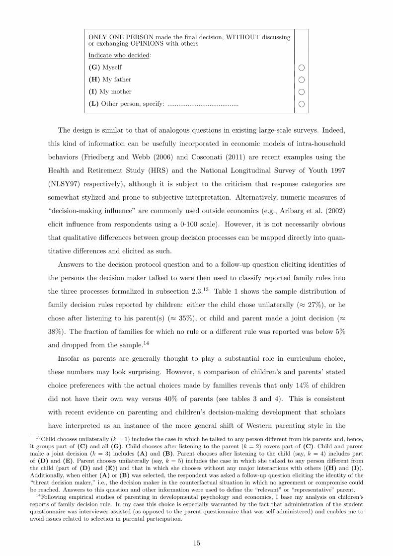
The design is similar to that of analogous questions in existing large-scale surveys. Indeed,

this kind of information can be usefully incorporated in economic models of intra-household

behaviors (Friedberg and Webb (2006) and Cosconati (2011) are recent examples using the

Health and Retirement Study (HRS) and the National Longitudinal Survey of Youth 1997

(NLSY97) respectively), although it is subject to the criticism that response categories are

somewhat stylized and prone to subjective interpretation. Alternatively, numeric measures of

“decision-making influence” are commonly used outside economics (e.g., Aribarg et al. (2002)

elicit influence from respondents using a 0-100 scale). However, it is not necessarily obvious

that qualitative differences between group decision processes can be mapped directly into quan-

titative differences and elicited as such.

Answers to the decision protocol question and to a follow-up question eliciting identities of

the persons the decision maker talked to were then used to classify reported family rules into

the three processes formalized in subsection 2.3.13 Table 1 shows the sample distribution of

family decision rules reported by children: either the child chose unilaterally (≈ 27%), or he

chose after listening to his parent(s) (≈ 35%), or child and parent made a joint decision (≈

38%). The fraction of families for which no rule or a different rule was reported was below 5%

and dropped from the sample.14

Insofar as parents are generally thought to play a substantial role in curriculum choice,

these numbers may look surprising. However, a comparison of children’s and parents’ stated

choice preferences with the actual choices made by families reveals that only 14% of children

did not have their own way versus 40% of parents (see tables 3 and 4). This is consistent

with recent evidence on parenting and children’s decision-making development that scholars

have interpreted as an instance of the more general shift of Western parenting style in the13Child chooses unilaterally (k = 1) includes the case in which he talked to any person different from his parents and, hence,

it groups part of (C) and all (G). Child chooses after listening to the parent (k = 2) covers part of (C). Child and parentmake a joint decision (k = 3) includes (A) and (B). Parent chooses after listening to the child (say, k = 4) includes partof (D) and (E). Parent chooses unilaterally (say, k = 5) includes the case in which she talked to any person different fromthe child (part of (D) and (E)) and that in which she chooses without any major interactions with others ((H) and (I)).Additionally, when either (A) or (B) was selected, the respondent was asked a follow-up question eliciting the identity of the“threat decision maker,” i.e., the decision maker in the counterfactual situation in which no agreement or compromise couldbe reached. Answers to this question and other information were used to define the “relevant” or “representative” parent.

14Following empirical studies of parenting in developmental psychology and economics, I base my analysis on children’sreports of family decision rule. In my case this choice is especially warranted by the fact that administration of the studentquestionnaire was interviewer-assisted (as opposed to the parent questionnaire that was self-administered) and enables me toavoid issues related to selection in parental participation.

15

last few decades towards a more open “affective and supportive” approach than the previous

“prescriptive and rigid” one (Provantini and Arcari, 2009). Alternatively, parents–especially

those with a higher socio-economic background and education–may just be “nudging” their

children’s choices in more subtle ways (similar to the rearing style of American middle-class

parents according to Lareau (2003)).

Stated Preferences and Junior High School Orientation. Respondents’ stated prefer-

ences were elicited by means of the following question, here reported with the wording used for

the child questionnaire. With the aim of making their individual pre-decision beliefs salient to

respondents when answering this question, in the actual questionnaire the question was placed

immediately after the battery of expectations questions used to estimate the behavioral models

(described in the paragraph “Probabilistic Expectations” below).

Try and think about your situation last year, when you where still attending your third

year of junior high school. [In the common introductory paragraph to expectations and stated

preference questions.] Please, RANK the following curricula from YOUR most preferred

one to the one you like the least, considering only YOUR preferences, expectations, and

the criteria YOU considered important for choosing among them. Start by assigning 1

to YOUR FAVORITE curriculum, then proceed by increments of 1 till YOUR LEAST

preferred one. The same number may not be assigned to two different schools.

Curriculum (either standard or laboratory) RankVocational - CommerceVocational - IndustrialTechnical - Commerce or SocialTechnical - IndustrialTechnical - SurveyorsArtistic EducationGeneral - HumanitiesGeneral - LanguagesGeneral - Learning or Social SciencesGeneral - Math and Sciences

Hence, for example, the survey task of a k = 2 child would entail retrieving his probabilistic

beliefs and his curriculum ranking (corresponding to those beliefs) before the choice, i.e., net

of any updating based on parental inputs.

In fact, set measurement issues aside, child and parent stated choice preferences will generally

not coincide with the family actual choices due to child-parent interaction in decision making.

In table 3, the proportion of families in which the final choice does not coincide with the child’s

stated preferred alternative is approximately 13-14% (columns 1 and 2). This figure is intuitively

smallest among families whose children reported making a unilateral decision (column 3), and

it increases slightly among families employing multilateral decision rules (columns 4 and 5). On

16

the other hand, actual choices and parents’ stated choice preferences do not coincide in 40% of

families (table 4). This percentage is, once again intuitively, highest among families in which

children reported making a unilateral choice and decreases conditional on more cooperative

protocols.

Admittedly, actual choices and children’s stated top-ranked alternatives do not coincide even

for the 11% of families whose children reported unilateral (self) decision (see table 3). Taking

the reported choice protocols at face value, this pattern may be explained by the existence of

some factors or constraints that affected the actual decision but were not accounted for in the

stated preference task (called “prominence” in the literature). For instance, figures in table 5

show that in about 60% of the cases in which child’s SP and RP do not coincide, the latter does

coincide with the orientation suggestion provided by junior high school teachers of the child.

Hence, one possibility is that, when reporting their choice preferences, some children abstracted

from the role that such a suggestion had in their choice. In the empirical analysis of section 4

I explore this possibility.

A separate interesting question is whether families employing joint decision making select

undominated alternatives, given individual members’ choice preferences. Table 6 shows that

cooperative families fail to select an undominated alternative in less than 5% of cases in my

sample, thereby supporting “group rationality.”

Probabilistic Expectations. From anecdotal and sociological evidence on curriculum choice

in Italy (Istituto IARD, 2001, 2005), I identified a set of outcomes, listed in the table below,

potentially important for this choice. Hence, after being prompted to think back to the previous

year before a final discussion and a final choice had been made, respondents were asked to report

on a 0-100 percent chance scale their subjective probabilities, {Pijn}i∈{c,p}, that outcomes

n = 1, ..., N would realize under the alternative scenarios that the child were to attend each

curriculum j = 1, ..., J of his choice set.15

15An additional question attempted to elicit children’s expected earnings at age 30 under the two alternative scenarios thatthey would start working immediately after graduation and that they would first obtain a college degree. However, responserates for these question were low, especially among children. Many of them did admit that they had no sense whatsoever of theorder of magnitude of a monthly salary. A minority provided answers based either on information received during orientationin junior high school or on their knowledge of their parents’ earnings. As for parents, a number of them left written notes onthe survey instrument explaining that, beyond the difficulty of providing any meaningful forecast, they did not regard sucha factor as particularly important for the choice. Be as it may, low response rates for these questions prevented inclusion ofexpected income in the empirical specification of child’s and parent’s expected utility functions.

17

Outcome Description

bj1 = 1 “Like”: The child will enjoy the core subjects of curriculum j.

bj2 = 1 “Ability-Effort I”: In curriculum j the child will spend ≥ 2.5h a daystudying or doing homework.

bj3 = 1 “Ability-Effort II”: The child will graduate from curriculum jin any length of time.

bj4 = 1 “Ability-Effort III”: The child will graduate from curriculum jin the regular time.

bj5 = 1 “Ability-Effort IV”: The child will graduate from curriculum jin the regular time and with a yearly GPA ≥ 7.5.

bj6 = 1 “Peers”: Attending curriculum j will enable the child to be in schoolwith his best friend(s).

bj7 = 1 “Flexibility I”: Attending curriculum j will enable the child to facea flexible college-work choice by providing him with a suitable trainingboth for some university field(s) and for work in some liked occupation(s).

bj8 = 1 “College”: The child will enroll in college, conditional on graduatingfrom curriculum j.

bj9 = 1 “Flexibility II”: Attending curriculum j will enable the child to facea flexible choice of field in college, i.e., to choose among a wide rangeof fields, conditional on graduating from j and on going to college.

bj10 = 1 “Work”: The child will find an acceptable and liked job after graduatingfrom curriculum j.

bj11 = 1 “Parent(s)”: The child will make his parent(s) happy by attending curriculum j.(Asked to the child only.)

As an illustration, I focus on the “objective outcome” bj5, which is one of special interest

since respondents’ probabilistic beliefs about its realization can be taken as their estimates of

the child’s curriculum j-specific ability combined with his effort.

For each curriculum listed below, please, answer the following percent chance question:

Last year, when you were still attending your third year of junior high school, what did

you think would be your percent chances of maintaining an YEARLY GPA of 7.5 or

HIGHER during your educational career, had you decided to attend that curriculum?

Figure 1 shows the distributions of responses for the vocational commerce and the general math-

and-science curricula in different estimation samples. As it is indeed observed in actuality (i.e,

based on realized students’ GPAs, though not on their passing and graduation rates), children

perceive the general math curriculum as more difficult than the vocational commerce one. This

can be seen by comparing the two top histograms, as low probabilities of obtaining a high GPA

in general math feature higher response frequencies than the corresponding ones for vocational

commerce, and viceversa. Moreover, higher frequencies for probabilities above equal chances

in the parental distribution of beliefs for general math (bottom right histogram) than in their

children’s distribution (bottom left histogram) are consistent with the common finding that

parents tend to be more optimistic regarding youths’ future (positive) outcomes than youths

are (e.g., Fischhoff et al. (2000), Dominitz et al. (2001), and Attanasio and Kaufmann (2010)).

18

A complete statistical description of expectations data is beyond the scope and space of this

paper, and can be found in Giustinelli (2010, Chpt. 2) for the original samples. There, I compare

moments of the sample distributions of probabilistic beliefs with local population statistics (and

with statistics from other studies) for outcomes for which such statistics are available (i.e., b2, b4,

b5, and b10). Despite substantial heterogeneity of beliefs across respondents and some evidence

of rounding and bunching at multiples of 5%, the mean and median responses match up fairly

well with the statistics used as comparisons, another typical finding in the literature employing

expectations data.

Unfortunately, beliefs on taste for subjects and on flexibility of future choices cannot be

easily related to objective statistics. Nonetheless, for the flexibility outcome b9 I was able to

compare respondents’ subjective beliefs with enrollment rates in different groups of fields by

graduation curriculum, where I take high school curricula followed by more disperse enrollment

distributions across college fields as those providing more choice in the college field decision.

Remarkably, subjective beliefs and statistics concord in identifying high school curricula that

provide more flexibility: the general math-and-science curriculum and, independent of the track,

any technology-oriented curriculum.16

4 Empirical Analysis

4.1 The “Unitary Family” Benchmark

Econometric Model. I use actual choices (RP data) together with children’s and, alter-

natively, parents’ probabilistic expectations to estimate two versions of a “unitary family”

benchmark model of curriculum choice. In the first, the child is the representative or relevant

decision maker (i.e., i ≡ c(f)); in the second, such a role is taken by the parent (i.e., i ≡ p(f)).

Assuming i.i.d. type-I extreme value random terms, the probability of observing child c from

family f attending curriculum j is

P(j|{{Pijn}Nn=1}10

j=1; {{αij}9j=1, {∆ui

n}Nn=1})

=exp

(µi[αi

j+∑N

n=1 Pijn ·∆uin

])∑10

j=1 exp(µi[αi

j +∑N

n=1 Pijn ·∆uin

]) , (4)

where αij is an alternative-specific constant measuring the average effect of all unincluded factors

and µi is the scale parameter inversely related to the variance of the error terms. Given

the parametric assumptions for the random terms and after setting αi10 = 0 as a location

normalization, the model’s coefficients, {αij}9j=1 and {∆ui

n}Nn=1 with i ∈ {c, p}, are identified

up to the scale factor, µi.16While this exercise reveals that flexibility and preferences for flexibility are modeled in a somewhat reduced-form manner

(see Barbera et al. (2004) for the theory), eliciting subjective probabilistic beliefs over all possible study and work pathsfollowing graduation from each high school curriculum in the choice set would have imposed an excessive response burden onrespondents in the context of the current study.

19

In practice, statistical identification of utility parameters relies on heterogeneity of decision

makers’ beliefs that function as alternative- and individual-specific attributes of the conditional

logit. Alternatively, under rational expectations, one could simply replace individual prob-

abilistic expectations with population averages disaggregated by individual characteristics, if

available. In fact, while estimation results from subjective expectations data could be easily

compared with those obtained imposing the assumption of rational expectations, the compari-

son would not provide a proper test for rational expectations, since there exist several reasons

why respondents may have expectations that differ from mean realizations in some population

or sub-population of reference. For instance, they may hold rational expectations but their

process may simply differ from the one characterizing the population taken as a reference by

the econometrician.17

Estimation of (4) from actual choices requires taking choice-based sampling into account. I

use Manski and Lerman (1977)’s weighted exogenous sampling maximum likelihood (WESML)

estimator (described in appendix A), on the ground that it is computationally tractable and pro-

vides a constrained best predictor of the discrete response even when the logit assumption is not

correct (Xie and Manski, 1989). This approach, however, requires knowledge of the population

enrollment shares for the school year 2007-2008 to calculate weights that make the likelihood

function behave asymptotically as under random sampling. I obtained this information from

the Provincial Agency for Education of Verona.

I additionally estimate (4) using children’s and parents’ stated preferences (SP data) as re-

sponse variables and compare the estimates thus obtained with those based on actual choices.18

In this case the sampling scheme can be thought of as equivalent to one of “intercept & follow”

with choice-based recruitment or interception. McFadden (1996) shows that for the basic case

without persistent heterogeneity across choice situations and for sole purpose of parameters’

estimation–as opposed to other population quantities whose recovery would still require re-

weighting–data from choice situations other than the interception can be treated in estimation

as if the sampling were random.19 This will naturally apply also to the joint SP-RP models

presented later, as made transparent by the formal framework for choice-based sampling with17Delavande (2008) provides an illustration and further discussion on this point. On the other hand, Li and Lee (2009)

are able to test and reject rational expectations in the context of political voting with social interactions, where voters’expectations are defined over the voting behaviors of the members of their reference group, demonstrating once again usefulnessof expectations data.

18It is important to clarify that estimates from the SP model should not necessarily be interpreted as strictly providing thetrade-offs children and parents will respectively make under unilateral decision making, for this would require that members offamilies employing multilateral decision rules (and non-decision makers of families using a unilateral rule) were presented witha counterfactual stated choice scenario explicitly worded in terms of individual decision-making. And it would also require thatdecision makers of families employing a unilateral decision rule were presented with a stated choice scenario making explicitreference to the actual choice situation. Yet, since children’s and parents’ SPs were elicited through a task that encouragedrespondents to recall their beliefs and preferences before the family choice process took place, SP data will contain usefulinformation on individual preference structures of children and parents over outcomes’ states.

19Notice also that because existing empirical evidence on SP models using ranking data supports significant differencesacross rank levels, with decreasing stability of ranking information as the rank of an alternative decreases (BenAkiva et al.,1991), I estimate the SP models using as an outcome variable the highest ranked curriculum only rather than the completeranking of alternatives.

20

multiple data sources presented in appendix A.

Revealed Preferences. Estimates of preference parameters for the basic benchmark model

with actual choices are shown in table 7. Significance levels are based on robust (“sandwich”)

asymptotic standard errors derived by Manski and Lerman (1977). (I discuss their validity

for statistical inference with my data in appendix B.1.) All specifications include alternative-

specific constants (estimates not shown for reasons of space), whose overall significance is con-

firmed by a Likelihood Ratio (LR) test. The adjusted LR index reported in the bottom row

of the table measures the percent increase in the value of the log-likelihood calculated at the

parameters’ estimates relative to its value under equal chances (i.e., no model), and it should

neither be interpreted as the R2 of a linear regression nor be used to compare specifications

that are not estimated on the same sample of data.

Estimates from children’s subjective expectations (columns 2-5) display the expected (posi-

tive) signs, perhaps with the exception of “average daily homework ≥ 2.5h” (b2), whose utility

coefficient may rather be hypothesized to be negative. The most important outcome is “child

likes the subjects” (b1), whose coefficient is approximately 2.5 times larger than that of “face a

flexible college field’s choice” (b9), 3.5 times larger than that of “graduate in the regular time”

(b4), and approximately 5 times larger than those of “find a liked job after graduation” (b10),

“attend college” (b8), and “face a flexible college-work choice” (b7). Preference parameters for

these outcomes are all significant at 1%, as opposed to that for “being in school with friends”

(b6) which, somewhat surprisingly, is barely significant.20

Qualitative results do not change when “make parent happy” (b11) is introduced in column

3, although the outcome itself turns out to be the third most important one after “child likes the

subjects” and “face a flexible college field choice.” Similarly, inclusion of a dummy capturing the

orientation suggestion by junior high school teachers (columns 4 and 5) induces only marginal

changes in the estimates, mostly by making the coefficient of the homework time’s outcome not

significant.21 However, the corresponding utility coefficient is significant and approximately 4

times smaller in magnitude than that of “child likes the subjects.” This is true despite the fact

that the information content of junior high school orientation suggestions should be incorpo-

rated in decision makers’ expectations. Hence, it is possible that orientation suggestions affect

curriculum choice through additional channels, e.g., indirectly, through choice set formation or,

directly, through preferences over outcomes.22

20Notice that while beliefs about friends’ choice behavior seems a potentially important variable to incorporate in a modelof curriculum choice, my model does not structurally allow for social interactions in the sense of Brock and Durlauf (2001).

21The orientation dummy is equal to 0 both when no suggestion was provided and when a track was suggested but nocurriculum was specified, and is equal to 1 otherwise. A version constraining the utility coefficient of the suggestion indicatorto 0 when the child (parent) received a suggestion but declared it was not considered in the choice produced results identicalto the ones shown. Sample size of columns 4 and 5 is lower than that of columns 2 and 3 because of item non-response on theorientation question.

22In fact, if the orientation suggestion consists of one or more specific alternatives a child may successfully pursue but lacksdetailed supporting motivations, families face an inferential problem similar to that faced by an econometrician trying to

21

Columns 6-7 display estimates from analogous specifications estimated using parental ex-

pectations. This model implies the same preference ranking over the most valued outcomes

as the model estimated using children’s expectations, thereby confirming the similarity of chil-

dren’s and parents’ beliefs documented in a preliminary descriptive analysis (Giustinelli, 2010,

Chpt. 2).

To ease comparison between children’s and parents’ preference weights, columns 8-13 display

estimates from the same specifications as in columns 2-7 but obtained from families in which

expectations were available for both child and parent. Since the estimated coefficients measure

the product of preference weights, {∆uin}Nn=1, and scale parameter, µi, a quick way to check

whether preference weights are likely to be similar between children and parents is to compare

ratios (between pairs of outcomes) of coefficients estimated from each group, since such ratios

are scale free.23 Overall, children’s expectations appear to have more explanatory power on

actual choices than those of their parents, consistent with the descriptive evidence presented

in subsection 3.2 that children had a more important role in the choice. In fact, the higher

level of significance of children’s expectations for almost all outcomes may also suggest greater

underlying heterogeneity in preferences among children.

Stated Preferences. Table 8 shows estimation results from SP data. A comparison with

the corresponding estimates based on RP data (e.g., columns 5 of tables 7 and 8) reveals that

the relative importance of different outcomes implied by children’s stated choice preferences

and by actual choices differ somewhat. For instance, outcomes related to future opportunities

and choices, such as finding a liked job after graduation and attending college, play a relatively

more important role in explaining stated preferences than actual choices, while the opposite is

true for some of the in-high-school outcomes, like graduating in the regular time. Moreover,

the model based on SP data detects positive preferences for being in school with friends, but

implies smaller weights on making parents happy and on the orientation suggestion.

For parents, too, the relative importance that the child will find a liked job upon graduation

and that he will face a flexible college-work choice are higher based on stated preferences (e.g.,

columns 7 of tables 8 and 7), while that of the orientation suggestion is lower. The coefficient

on homework time is now intuitively negative but, curiously, only among parents (although not

statistically significant). Moreover, parents do not seem to assign a significantly positive weight

on their children being in school with friends based on their stated preferences.

recover decision makers’ beliefs and preference parameters from choices. On the one hand, this implies that family membersmay have only noisy measures of teachers’ opinions available to update their own beliefs. On the other hand, if teachers wereto base their suggestions not only on children’s abilities and aptitudes but also on children’s intentions and choice preferencesinclusion of the orientation dummy would be problematic to start with.

23Estimates of preference parameters from children’s and parents’ expectations and for different samples may be alsoevaluated and compared in terms of the change they imply in predicted choice probabilities when expectations for specificoutcomes and alternatives change marginally. These calculations are not shown for reasons of space, but are available uponrequests. On the other hand, high non-response rates to the expected earnings’ questions prevent me from including thatvariable and from making willingness-to-pay calculations based on its utility coefficient.

22

Overall, ratios of preference parameters for pairs of outcomes display some variability both

between children and parents and across data sources, suggesting that the corresponding differ-

ences in estimated coefficients are not a pure artifact of heterogeneous variance of unobserved

factors across groups and data sources. Put differently, under the assumption of no bias in SP

responses (discussed in appendix B.2.1), it seems reasonable to hypothesize that utility param-

eters estimated from actual choices and children’s (or parents’) expectations will capture both

preferences and decision-making interactions.

Moreover, as discussed in subsection 2.3, even when children and parents are aligned in

theirs beliefs, preferences, or both, prediction and counterfactual analysis still require that

family decisions be analyzed through a model that specifies the correct decision-making unit

and protocol. Therefore, motivated by this idea, in the next subsections I pool RP and SP

data together, and I exploit their distinct information contents together with information on

family decision rules to gain identification power and separate parameters describing the latter

from children’s and parents’ utility weights. Specifically, I estimate a distinct discrete choice

model for each observed family decision rule, thus making the conceptual framework presented

in subsection 2.3 operational.

Heterogeneity. While I do necessarily impose restrictions on preference parameters between

SP and RP models within family decision protocols, I do not impose any restriction on preference

parameters across models describing different protocols. This is because child and parent

preference structures are likely to vary across families employing different decision rules, as

suggested by raw correlations between observed family protocols and actual choices in the

data.24

Preference heterogeneity between children and parents and across decision rules are the only

forms of systematic or observed heterogeneity I explore in this paper. Of course, it is possible

that preferences over outcomes’ states vary with decision makers’ characteristics, such as gender

and family background, and even with their beliefs. While there would be neither conceptual

nor computational difficulties in introducing systematic heterogeneity by assuming a functional

form that specifies how individual characteristics enter the structural parameters, because of

the relatively small sample sizes available for estimation of the protocol-specific models relative

to the already large number of estimated parameters, I prefer not to pursue this line. This

notwithstanding, given the correlation pattern existing between family decision rules, actual

choices, and background characteristics, allowing for heterogeneous family rules will provide in

itself indirect evidence about preference heterogeneity across the latter.25

24In fact, imposing homogeneous preferences for children and parents across decision protocols would actually strengthenidentification, possibly allowing me to analyze empirically the more general model in (3). In such a case preference parameterswould be identified from variation in children’s and parents’ beliefs from k = 1 families, whereas beliefs’ and preferences’aggregation parameters would be respectively identified from differences between stated preferences and actual choices ofk = 2 and k = 3 families. An obstacle to this approach, however, is that response rate is low among k = 1 parents.

25A discrete choice model may additionally feature forms of unobserved heterogeneity that, if present, will generate correla-

23

4.2 Heterogeneous Decision Protocols

4.2.1 Econometric Models

Child Chooses Unilaterally (k = 1). Taking information of family decision rules at face

value, if a child reports making curriculum choice without any interactions with his parents,

only his expectations and preferences are relevant for the final choice. Hence, a first natural

approach is to estimate children’s preference parameters from their expectations and actual

choices (or/and stated preferences), as follows.

• Model with One Data Source. This model is formally equivalent to the unitary bench-

mark in (4), with i ≡ c(f), but is estimated on the subsample of children that reported

making a unilateral choice. That is,

maxj∈J

Γ1fj ≡ EU

t,1cj = αt,1

j +N∑

n=1

Pcjn ·∆uc,t,1n + εt,1cj , (5)

where εt,1cj is i.i.d. type-I extreme value, with scale parameters µt,1 and t ∈ {RP,SP}.

Alternatively, SP and RP data can be combined to increase estimates’ precision while gaining

insight on possible differences between the two data generating processes.

• SP-RP Joint Model. The model is(RP, 1) : Γ1

fj ≡ EURP,1cj = αRP,1

j +∑N

n=1 Pcjn ·∆uc,1n + εRP,1

fj

(SP, 1) : EUSP,1cy = αSP,1

y +∑N

n=1 Pcyn ·∆uc,1n + εSP,1

cy ,(6)

where j indexes actual choices (RP) and y indexes stated choice preferences (SP), with

j, y ∈ J . εRP,1fj and εSP,1

cy are i.i.d. type-I extreme value, with scale parameters µRP,1 and

µc,SP,1 respectively. With no serial correlation between SP and RP error components, the

resulting log-likelihood of observing the RP-SP pair (j, y) is the sum of the log-likelihoods

of j and y, the former corrected for choice-based sampling (shown in appendix A).

The main difference between (6) and (5) is that the common component of the systematic

portions of RP and SP utilities (i.e.,∑

n Pcjn ·∆uc,1n ) enables identification and estimation of the

SP-RP scales’ ratio, µ1 = µc,SP,1/µRP,1. Specifically, because Var(εRP,1fj ) = (µ1)2 · Var(εSP,1

cy ),

estimate of µ1 can be used to investigate whether the two sources of data have approximately

the same amount of random noise by testing µ1 = 1. In turn, testing equality of the RP and

SP alternative-specific constants provides additional information on the relationship between

RP and SP unobservables, since they capture the average effects of all unobserved factors.

tion across the alternatives’ random utility components and cause the i.i.d. assumption to fail. In appendix B.2.2 I discuss apotential source of unobserved heterogeneity that is specific of SP-RP (and repeated SP and other logitudinal) settings, i.e.,unobservable persistence across data sources.

24

Child Chooses After Listening to the Parent (k = 2). The system of latent expected

utilities is now(RP, 2) : Γ2

fj ≡ EURP,2cj = αRP,2

j +∑N

n=1

[wc,2

n · Pcjn + (1− wc,2n ) · Ppjn

]·∆uc,2

n + εRP,2fj

(c-SP, 2) : EUSP,2cy = αSP,2

y +∑N

n=1 Pcyn ·∆uc,2n + εSP,2

cy ,

(7)

where j, y ∈ J and εRP,2fj and εSP,2

cy are i.i.d. type-I extreme value with scale parameters µRP,2

and µc,SP,2 and no serial correlation between SP and RP. Parent’s preferences, instead, are

estimated from a standard SP model,

(p-SP, 2) : EUSP,2ph = αSP,2

h +N∑

n=1

Pphn ·∆up,2n + εSP,2

ph , (8)

with h ∈ J .

Children’s preference weights, {∆uc,2n }Nn=1, are identified from variation in children’s expecta-

tions, through the SP component of the model (c-SP,2). The equality constraints on preference

parameters between (c-SP,2) and (RP,2) and the add-to-one restrictions on the aggregation

weights for each outcome allow one to back up the latter set of parameters, {wc,2n }Nn=1, from the

RP model.26 In fact, whether one is able to pin these weights down with some precision will

generally depend on how much variability exists both in child-parent expectations’ differences

and between children’s stated preferences and observed choices across families. Once again,

combination of SP and RP data yields identification of the SP-RP relative scale, µ2.

Child and Parent Make a Joint Decision (k = 3). In this model child and parent aggre-

gate their expected utilities outcome by outcome but without distinction between expectations’

revision and negotiation over preferences. That is,

(RP, 3) : Γ3fj ≡ EU

RP,3cj = αRP,3

j +∑N

n=1 φc,3n ·

[Pcjn ·∆uc,3

n

]+ (1− φc,3

n ) ·[Ppjn ·∆up,3

n

]+ εRP,3

fj

(c-SP, 3) : EUSP,3cy = αc,SP,3

y +∑N

n=1 Pcyn ·∆uc,3n + εSP,3

cy

(p-SP, 3) : EUSP,3ph = αp,SP,3

h +∑N

n=1 Pphn ·∆up,3n + εSP,3

ph ,

(9)

with j, y, h ∈ J . εRP,2fj , εSP,3

cy and εSP,3ph are i.i.d. type-I extreme value with scale parameters

µRP,3, µc,SP,3, and µp,SP,3 and no serial correlation across data sources. The identification

argument for (9) is analogous to that of (7), but it requires the additional restriction of equal

relative scales for (c-SP,3) and (p-SP,3).

26Taking ratios of SP and RP utility coefficients separates {wc,2n ·µ2}Nn=1 and {(1−wc,2

n ) ·µ2}Nn=1 from {∆uc,2n }Nn=1. Further

taking ratios between {wc,2n · µ2}Nn=1 and {(1− wc,2

n ) · µ2}Nn=1 for each outcome isolates {wc,2n }Nn=1.

25

4.2.2 Estimation Results

Children’s preferences are displayed by decision protocol in tables 9, 10, and 12 and 13, which

also include estimates of the protocol weights. Whereas parents’ preferences, shown in tables

11, 12, and 13, are estimated for groups k ∈ {2, 3} only, because of low participation of k = 1

parents.

Preference weights. Starting with the in-high-school outcomes, taste or preference for sub-

jects is confirmed to be the most valued outcome by both children and parents, as well as across

decision protocol groups and data sources.

The difference in utility generated by the prospect of having to study and to do homework

for at least 2.5 hours daily versus not having to is negative for the k = 1 children and positive,

but not significant, for the other two groups. This coefficient is negative also among k ∈ {2, 3}

parents, but it is not significant. Because the k = 1 subsample is more populated by male

children attending curricula with longer school hours, less homework and home study time, and

more manual laboratory classes (e.g., the vocational and technical industrial and the artistic

tracks), this pattern is suggestive of differential preferences for these kinds of schedule and

activities as well as gender differences.

The importance rank of graduating in the regular time, between 3rd and 5th among all

outcomes, is fairly stable across protocol groups; however, its relative magnitude (with respect

to taste for subjects) is highest in the k = 2 group and lowest in the k = 1 group. Again, this

may be capturing differential preferences for a regular path among high ability students and

girls, more represented in the k = 2 group (see table 2). On the contrary, this outcome does not

appear to be particularly important for parents, since its coefficient is not significantly different

from 0 in all specifications and groups.

As for being in school with friends, its utility weight is positive among children and negative

among parents for most specifications, but it is never significant. Finally, when the outcome

“make (the relevant) parent happy” is introduced, qualitative results do not change and, as for

the benchmark model, the coefficient for this outcome is always positive and usually significant.

Its relative importance, however, vary across protocol groups, being substantially higher among

k = 1 children. Hence, to the extent that children have some knowledge, albeit imperfect, of

their parents’ preferences, this suggests that even k = 1 parents are likely to play a relevant

role in their children’s choice, perhaps more indirectly.

Moving to outcomes capturing choices and opportunities after graduation from high school,

k = 2 children display a relatively strong preference for being able to make a flexible college

field choice, second most important outcome to them after like the subjects, followed by find a

liked job after graduation and make a flexible college-work choice. k = 3 children, too, place

a high preference on making a flexible college field choice, whose coefficient is comparable in

26

magnitude to that of attending college. This pattern seems intuitive, given that these two

groups are made of relatively high ability and high socio-economic background students, more

concentrated in general curricula (see table 2). Less intuitive is the fact that parents assign

higher importance ranks and relatively higher weights to finding a liked job immediately after

graduation and to making a flexible college-work choice than to making a flexible college field

choice and to attending college, respectively.

The picture for k = 1 children is somewhat more complex. On the one hand, their SPs imply

a strong and intuitive preference for finding a liked job immediately after graduation. On the

other hand, estimates obtained from RP data generate significant utility weights on attending

college, followed by making a flexible college-work choice, and a non-significant coefficient for

finding a liked job immediately after graduation. When combining SP and RP data and letting

preference coefficients vary across data sources one outcome at the time, I generally cannot reject

the null hypothesis of equal SP and RP coefficients based on an LR test, with the exceptions of

making a flexible college field choice (b9) and finding a liked job after graduation (b10). Hence,

in columns 11 and 13 of table 9 (specifications S5 and S6 respectively) I allow coefficients of

both b9 and b10 to vary between (RP,1) and (SP,1), while constraining the remaining ones to

be equal in the two models. A LR test rejects the fully constrained specifications S2 and S4 in

favor of S5 and S6.27

Another difference between RP and SP for group k = 1 concerns the orientation suggestion.

As suggested by the descriptive evidence shown in subsection 3.2, the RP model implies a

stronger role for the orientation dummy, whose coefficient is approximately twice as large as

that implied by the SP data. Even larger differences are observed for the other two groups

(k ∈ {2, 3}), where the orientation dummy is usually not significantly different from 0 in the

SP component of the model.

Because the same expectations data are used to estimate the SP and RP utility parameters,

this finding suggests the existence of an additional channel, beyond that of expectations, through

which the orientation suggestion affect actual choices but not stated preferences. As previously

mentioned, this channel could be preferences directly or could be a separate stage of choice set

formation. The former may occur if, for instance, teachers publicize “institutionally approved”

criteria of curriculum choice (e.g., “children should focus on their attitudes without letting

themselves being influenced by their friends’ choices”), thereby offering second-order preferences

that children can adopt through a process of alignment of their first-order preferences to them.

Of course this requires relaxation of the assumption that individuals’ preference structures are27A possible explanation is what the SP literature calls “prominence,” i.e., respondents’ tendency to focus only on few most

important attributes or not to consider situational constraints when responding stated choice questions. While prominencewould seem more likely to occur in stated choice tasks with hypothetical scenarios or in the kinds of SP-off-RP experimentsanalyzed by Train and Wilson (2008), here it would imply that SPs and RPs do not coincide in more cases than they should.Hence, if present, this type of response bias would go in the opposite direction than the “inertia or justification bias” generated,e.g., by mechanisms of ex-post rationalization (discussed in appendix B.2.1).

27

hardwired and cannot be manipulated via policies enacted by socialization agents (see Karniol

(2010) for a theory of socialization that develops this idea). The latter may occur if teachers’

opinions and recommendations affect choice sets used by families in the choice by inducing

them to consider alternatives that they would not consider otherwise or to drop alternatives

that they would seriously consider in the choice.28

Differences between the data generating processes of SP and RP can be further investigated

by inspection of the SP/RP scale parameter and of the alternative-specific constants of the two

models. On the one hand, for the k = 1 group I cannot reject the hypothesis that µ1 = 1 nor

a model with the RP and SP constants constrained to be equal to one another by alternative.

These findings indicate that for the group of children that reported making a unilateral decision

the unobservable processes underlying RP and SP are reassuringly similar. On the other hand,

µ2 and µ3 are significantly different from 1 in all specifications and range from 0.45 to 0.65,

meaning that the variance of the unobserved components of the SP model is between 2.5 and

5 times larger than the variance of the RP model.

A larger SP variance is a common finding in the SP-RP empirical literature (Morikawa, 1994).

This is not surprising, since SP data are usually elicited from stated choice experiments under

hypothetical scenarios in which respondents generally have only a subset of the information

they would have in actual choice situations. Hence, as pointed out by Manski (1999), stated

choice experiments tend to elicit preferences mixed with individual expectations of events that

may affect choice behavior and are not included in the proposed scenario. While in my setting

the SP task in one of recall and not one of choice under a hypothetical, it is possible that the

additional noise is indeed related to the mental process of recall and abstraction respondents

were required to perform. (For related issues concerning sp-off-rp experiments see also Train

and Wilson (2008).)

Protocol weights. Inspection of the top panel of table 10 reveals that variability of child-

parent expectations’ differences pins down child’s weights on parental expectations, { 1− wc,2n }Nn=1,

with some precision only for few outcomes. For instance, children assign a greater weight on

their parents’ opinions than on their own about graduating in the regular time, thereby trusting

parental assessments of their ability and effort better than theirs. The estimated weight for

this outcome ranges from 0.626 to 1.120, depending on the specification; however, all values

between 0.5 and 1 are compatible with the estimates, and for some specifications even a weight

of 0 cannot be rejected.

The weight on child’s preference for subjects is estimated precisely and lies between 0.411

and 0.457. The hypothesis of equal weights cannot be rejected, while 0 and 1 are rejected28Endogeneity of the orientation dummy may be an alternative or additional explanation. However, if SP data are measured

with sufficient accuracy the endogeneity effect should show up also in the SP model, which does not seem to occur at least forthe k ∈ {2, 3} groups.

28

for all specifications. The weight on making a flexible college field choice, instead, favors

child’s opinion, and values above 0.5 can generally be rejected. As for the remaining outcomes,

weights are estimated imprecisely and are, therefore, compatible with any value between 0 and

1. Despite this, a model with equal weights across outcomes is rejected for all specifications.

Estimates for the k = 3 group in top panel of table 12 refer to the weights on children’s

utility components, {φc,3n }Nn=1. The weight on child likes the subjects ranges between 0.15 and

0.3. A weight of 0 is rejected for all specifications, and similarly for any weight greater or

equal to 0.5. On the contrary, weights on making a flexible college field choice and on finding

a liked job after graduation are favor the child; however, only values close to 0 can be rejected,

given estimates’ precision. Estimated weights for the remaining outcomes are imprecise and

compatible with a large range of values, including 0 and 1.

For this group I cannot reject the null hypothesis of a unique weight aggregating child’s and

parent’s expected utilities. Estimates for the constrained model are shown in table 13. The

estimated weight on child’s utility, which ranges between 0.295 and 0.370, is fairly precise; both

0 and values of 0.5 or above are rejected. This confirm the important explicit role of the k = 3

parents in their children’s curriculum choice.

Of course, these estimates rely on the decision-making unit and decision process being cor-

rectly specified. To shed some light on potential misspecifications, I test the multilateral deci-

sion models against the unilateral model and against one another. Since the unilateral model

is nested in both multilateral models, I perform LR tests for whether all weights on parental

beliefs are equal 0 in table 10 and for whether the weight on child’s expected utility is equal 1

in table 13. The null hypothesis is rejected in both cases.

I finally estimate the specification in which the child chooses after listening to the parent on

the k = 3 subsample and I compare it with the child-parent joint decision model, and viceversa

for the k = 2 subsample. Since the two models are not nested, I use the test presented in Ben-

Akiva and Lerman (1985, p. 171-174) that compares the adjusted LR indeces of the two models

being tested, i.e., P(ρ2

B − ρ2A > z

)≥ Φ{−[2 ·N · z · ln(J) + (KB −KA)]1/2} with z > 0, where

all N observations in the sample have all J alternatives and KA and KB are the number of

parameters of the two models. Based on this test, the specification in which the child chooses

after listening to the parent is found to be statistically superior for both k = 2 and k = 3

groups.29

29In fact, a comparison of reported family decision rules by children and by parents reveals less agreement (and hence higherrisk of missclassification) in distinguishing between rules 2 and 3 than between rule 1 versus the others (see Giustinelli (2010,Chpt. 2) for more details).

29

5 Counterfactual Analysis

Galileo and Michelangelo, Resumed. In this paper I maintain the standard assumption

that preferences used to trade off different outcomes’ states are hardwired and cannot be ma-

nipulated by policies. On the contrary, tastes or preferences for curricula’s core subjects are

uncertain in the model, and individuals hold subjective beliefs on them. It is therefore possi-

ble that “awareness” or “desensitization” campaigns can influence choice behavior by affecting

beliefs on taste. Hence, in table 14 I simulate two scenarios in which individual subjective

probabilities that the child will like the subjects of a specific curriculum change by a fixed

amount.

Specifically, in the top panel I calculate the percent changes in predicted enrollment shares

following a 0.1 increase in the subjective probabilities (of children, parents, and both) that the

child would enjoy the core subjects of the math-and-sciences curriculum (policy 1). Whereas,

in the bottom panel I report the corresponding changes following a 0.1 drop in the probabilities

that the child would like the subjects of the artistic curriculum (policy 2). Calculations are

done separately for the pooled samples (unitary models) and for the different decision protocol

groups (protocol-specific models).

These policies generate, for all groups and models, an intuitive increase of the probability

of enrolling in the math-and-science curriculum and a drop of the art enrollment probability.

Choice probabilities of all other curricula display the opposite pattern. Such changes, however,

are heterogeneous across models and targeted recipients, suggesting that decision-making pro-

tocol and identity of the targeted group(s) matters. For instance, assuming a unitary model

with parents as representative decision makers sizeably overestimates the magnitude of enroll-

ment response to awareness and desensitization campaigns implied by the heterogenous model

(+18.93 vs. +12.07 for math-and-science awareness, and -18.91% vs. -13.28% for art desen-

sitization). Whereas a unitary model based on children’s expectations generates much closer

predictions (+11.16% vs. +12.07 and -13.77% vs. -13.28%, respectively).

Publication of Education Statistics. I then simulate policies that make curriculum-specific

statistics available to families.30 Specifically, in the top panel of table 15 I calculate the per-

cent changes in predicted enrollment probabilities following publication of the 2006 high school

graduation rates by curriculum of graduation (conditional on a regular path) based on Al-30This is similar in spirit to existing works in economics of education that analyze the effect on parents’ school choices of

disclosure of information on school-level characteristics, such as school test scores (see Hastings and Weinstein (2008) for anapplication exploiting both a natural and a field experiments). Indeed, most high schools in Verona, and in Italy more generally,have public web-pages where some of them post, among other information, school-level statistics for previous cohorts (e.g.,passing rates between grades) and post-graduation outcomes (e.g., college enrollment by field and job placement by sector). Ofcourse, while statistics summarizing outcomes of previous cohorts by chosen action constitute in principle useful information,in practice decision makers attempting to use such information face, as econometricians would, the identification problemknown as selection (see analysis by Manski (2004b)).

30

maDiploma (2007a)’s statistics (policy 3).31 And in the top panel of Table 16 I show percent

changes in predicted enrollment probabilities following disclosure of the AlmaDiploma (2007b)’s

statistics on 2006 college enrollment by graduation curriculum (policy 5). These statistics are

the most recent ones that could have been made available to families of my sample, whose

children entered high school in Fall 2007.

Policy 3 generates a moderate increase in predicted enrollment in general curricula, espe-

cially the humanities and math, and a drop in predicted enrollment in the vocational and artistic

curricula. While this pattern is suggestive of a potential overstatement of the difficulty levels

of general curricula, the protocol-specific predictions show an intuitive attenuated pattern for

the k = 2 group, especially the children, which is probably due to selection of girls and higher

socio-economic background/higher ability children into this group (see table 2). In turn, policy

5 generates qualitatively similar predictions, this time suggesting a potential underestimation

of the “costs” of going to college after receiving a not fully suitable training.32

Last but not least, decomposition of counterfactual enrollment responses by decision-making

rule for these experiments shows that publication of education statistics would have a larger

impact on the group of children reporting unilateral decision by self. While this cannot be nec-

essarily taken as a sign that these children have less precise beliefs, this is indeed one possibility.

Of course this may be either due to differential observable or unobservable characteristics of

children across protocol groups (such as ability or access to information) or to the very decision

protocol (or to both). In particular, families in which parents have a greater involvement in

their children’s choice may be relying more on statistics and on other “hard” information from

teachers, schools, and orientation (see Adams and Ferreira (2010) for a similar argument about

individual vs. multilateral decision, but in a different context).

Institutional Policies. In the bottom panels of tables 15 and 16 I simulate the effects of

changes in families’ beliefs generated by two institutional-type policies. Policy 4 lowers ed-

ucational standards and equalizes them across curricula by guaranteeing all children a pass

in all grades through the diploma for all curricula.33 In practice, I assume that individuals

hold subjective probabilities that the child will graduate in the regular time equal to 1 for all

curricula, keeping expectations for the other outcomes fixed.31AlmaDiploma is a consortium that collects data on attainment, college, and labor market outcomes of high school graduates

in Italy with the aims of providing them with college orientation services and of facilitating matching of labor demand andlabor supply for high school graduates (see http://www.almadiploma.it).

32A limitation of this counterfactual experiment is that, although these statistics are curriculum specific, they are notdisaggregated by individuals’ characteristics, such as gender or academic ability (see Sartarelli (2011) for an argument infavor of disclosure of conditional statistics in the context of college major choice). More generally, the exercise assumes thatdisclosed statistics are taken and used by decision makers at face value, since no model of expectations’ formation and updatingis specified and estimated.

33While taken literally this policy may appear unrealistic and probably not desirable, its dynamics are similar to thosegenerated by the introduction of “educational debits” or “fail credits” by the Law 425-1997, subsequently modified by the Law1-2007. De facto this system enabled children with grades below the passing level in one or more subjects to progress throughschool grades by contracting “educational debits” that could be (easily) cleared at some later time.

31

Policy 6, instead, strengthens specialization by preventing access to university following any

diploma of the vocational type, similar to the Italian secondary system before the 1969 reform

that opened university access to students graduating from technical and vocational schools. In

the simulation I assume that individuals hold zero subjective probabilities of going to college,

of facing a flexible college-work choice, and of facing a flexible choice of field in college after

graduating from any vocational curriculum.

As expected, the first intervention tends to stimulate enrollment in general curricula and

in some technical curricula while depressing enrollment in vocational and artistic curricula.

But responses do not seem large. Once again the pattern is attenuated, and in some cases

reversed, among the k = 2 children who are likely the least “ability constrained.” In turn, the

second intervention induces a huge drop in vocational enrollment, mostly in favor of technical

schools. The latter result is intuitive: children who value the possibility of going to college

after graduation, but that would enroll in a vocational curriculum if the restriction were not in

place, would now switch to curricula of the “lowest” track that ensures eligibility for enrolling in

college. Finally, the decomposition by decision protocol shows that if parents only were aware

of policies changing institutional features of tracking, the impact of such policies may be much

smaller than it would be if children, too, were informed.

6 Relationship with Existing Research

6.1 Curricular Stratification, Intergenerational Transmission, and Career

Decisions under Uncertainty

Most schooling systems feature some form of stratification or tracking, which can be by ability

(as in the U.S.), curricular, or a combination of the two (as in many European countries).

The distinctive purpose of the latter is to provide educational specialization so that children

with different aptitudes and aspirations may pursue careers in different areas and requiring

different types of expertise. Yet, significant cross-country variation exists in how stratification

is implemented, depending on its time, the allocation mechanism of children into tracks, and

the extent of specialization and separation of different tracks.34 In turn, these variables are the

main determinants of the (form and degree of) uncertainty faced by families regarding their

children’s education paths and future outcomes: On one side, the earlier the child’s age at34There exists a sizeable literature in economics of education concerned with how institutional features of a stratified

schooling system affects its efficiency (e.g., Ariga et al. (2010)) and equity (e.g., Brunello and Checchi (2007)). Prominentissues analyzed by this literature are the tension between breadth and depth of education and the determination of the optimaltime of tracking (e.g., Brunello et al. (2007)). In the OECD group, for instance, the age of first tracking ranges from 10 inAustria and Germany to 18 in Canada and the U.S., and 15-16 are modal (Brunello and Checchi, 2007). In fact, the Americansystem is considered to be de-tracked curricular-wise, though recently some states have experienced specialization shifts, suchas the Florida requirement that 9th graders declare a major (I thank David Figlio for pointing this out). As for the sortingmechanism, typical ones are testing (e.g., in Germany) and family choice (e.g., in Italy). As for the degree of rigidity, afully rigid stratification (as in Germany) is characterized by the impossibility of switching between tracks during compulsoryeducation and by barriers to college enrollment following graduation from “lower” vocational-type tracks.

32

tracking the longer the future that must be anticipated and the less the accumulated history

of past school performance that can be used to form expectations on the child’s tastes, ability,

and future outcomes. On the other side, the stronger and more rigid is specialization the more

difficult are “wrong choices” to be costlessly corrected or corrected at all.

The Italian system considered in this paper constitutes an interesting hybrid characterized

by a relative early tracking (at entry in high school) that is, in principle, mitigated by family

choice as a sorting device and by flexibility mechanisms enabling both track switching during

high school (passerelle or “bridges”) and enrollment in university following any 5-year diploma

from any track. Based on anecdotal and sociological evidence (e.g., Istituto IARD (2001,

2005)), however, Italian families (especially the children) seem to believe that a wrong training

in high school will generally carry a “cost” in form of an inadequate preparation for college (or

work) and unfavorably perceive track switching as likely yielding a longer time to graduation.

Hence, these flexibility mechanisms do not appear to unambiguously reduce the uncertainty

accompanying an early curricular stratification.

As a matter of fact, tracking during compulsory education renders curriculum choice a

(early) career decision that, as such, requires a large investment in training and is per se

characterized by uncertainty on individual ability and investment returns (e.g., Altonji (1993)

and Arcidiacono (2004)). My work contributes to existing empirical studies of curriculum choice

with early curricular stratification (e.g., Checchi and Flabbi (2007)) by modeling uncertainty

explicitly, but without imposing strong assumptions on how youths and their parents form

expectations on future choice-related outcomes (see Manski (1993) and references therein).

Moreover, such a structural albeit simple framework enables me to perform novel counterfactual

exercises simulating the effects on curriculum enrollment of policies involving publication of

information aiming at reducing families’ uncertainty and modification of variables regulating

rigidity and standards of stratification.

Some scholars have further claimed that track choice by families (as opposed to testing) ul-

timately translates into a greater dependence of children’s paths on family background, thereby

hampering intergenerational mobility (Checchi and Flabbi, 2007). According to this view, cur-

riculum choice may be a channel through which parents end up creating their children in their

own image (a la Bisin and Verdier (2001)) rather than improving their children’s condition (as

in Doepke and Zilibotti (2008)). However, while intergenerational transmission of preferences

and beliefs from parents to children is commonly considered to be the main vehicle for either

possibilities, very little is known in practice of how children and parents perceive uncertain

dimensions of curriculum choice and of what roles children and parents play in it. Hence, the

main contribution of the data collection and the empirical analysis carried by this work is clearly

to provide new and more rigorous and detailed evidence on some these issues.35

35Saez-Marti and Zilibotti (2008) review the cultural transmission-endogenous preference literature and summarize the two

33

6.2 Parenting and Decision Making by Children

As just mentioned, the literature on curriculum choice posits a crucial role of family background

(Checchi and Flabbi, 2007). Despite this, to the best of my knowledge no existing study has

explicitly modeled the roles of children and parents in the choice. For instance, Arcidiacono

et al. (2011) and Zafar (2008) estimate models of college major choice under uncertainty using

measures of subjective probabilities and counterfactuals from students of two top American

universities. Both works assume that college students are the main decision makers of their

major, which appears sensible given the latter’s age. And yet, based on data on perceived

(by students) parental approval and expectations, Zafar (2008, 2011) finds evidence of a likely

strong parental influence in the choice. In turn, Attanasio and Kaufmann (2010) analyze high

school and college enrollment decisions in rural Mexico with data from Progresa and find that

both children’s and parents’ expectations matter for the former, while only youths’ expectations

are relevant for the latter. However, they do not model child-parent interaction explicitly.

In truth, identification of a proper decision-making unit for this type of choice is not at all

unambiguous. The main difficulty is that, on the one hand, adolescents undergo development

of their preferences and capabilities for communication, formal reasoning, and independent ac-

tion; on the other hand, they still rely on parental guidance and support. In particular, while

adolescents appear old enough to play an active role in their schooling decisions, their level

and rate of autonomy acquisition will generally vary with their traits, ability, environment, as

well as parental preferences, resources, and parenting style (see Lundberg et al. (2009) and

reference therein from developmental psychology). It seems, therefore, natural to hypothe-

size existence of heterogeneous decision rules across families, ranging from unilateral to more

interacted protocols.

Despite this fact, to date only a recent handful of studies, such as Bursztyn and Coffman

(2011) and Berry (2010), have challenged the unitary view of household behavior (Becker,

1981) in the context of educational choices. These works develop non-cooperative models of

child-parent interactions with moral hazard motivating empirical applications on children’s

school attendance (or achievement) using data from field experiments in developing countries.

Specifically, Bursztyn and Coffman (2011) analyze adolescents’ school attendance in Brazilian

favelas and provide evidence that child-parent conflicts play an important role via the parents’

difficulty of monitoring their children’s actions. Whereas Berry (2010) tests whether identity of

main modeling approaches. In the paternalistic model parents use their own preferences to evaluate their children’s utilityand, with some effort, seek to transmit their preference trait to the latter (as in Bisin and Verdier (2001)). Whereas, in thenon-paternalistic model (e.g., Doepke and Zilibotti (2008)), parents choose their children’s preferences to maximize children’swell-being by making a costly investment, but without necessarily trying to install their own cultural variant. My frameworkincorporates both non-paternalistic and paternalistic features. On the one hand, parents and children share the same objectivefunction, i.e., choosing the curriculum that matches the child best while accounting for both early and later future consequencesof this choice. And, with this very purpose, parents may try to affect children’s choice (and future) via the channels of beliefs’transmission or of a negotiated choice. On the other hand, parents’ intervention is based on their own beliefs and preferencesover future states, which are allowed to differ from those of their children.

34

recipients (i.e., children or parents) of cash incentives for school achievement (e.g., enrollment

and attendance) in India affects their effectiveness.36

My paper contributes to this stream of works by analyzing a different schooling choice

margin (i.e., “quality” vs. “quantity” of human capital, although the two are clearly related in

a stratified context) and by explicitly modeling child-parent decision making with heterogeneous

cooperative-type rules. The latter choice is justified by the fact that in my setting children and

parents are assumed to solve the very same problem. Thus, even though in this paper I do not

model family selection into decision rules, which I take as exogenously given, the underlying idea

is that cooperation exists whenever communication of opinions, information, and preferences

can improve quality of choice.37

7 Conclusions

In this paper I study the empirical identification of a framework of static decision making under

uncertainty with multiple decision makers and no strategic interactions that combines elements

of Savage (1954)’s setup, Harsanyi (1955)’s utilitarian aggregation, and Raiffa (1968)’s experts

problem. The identification problem is one of distinguishing how decision makers’ beliefs and

preferences over outcomes’ states and their decision rule determine actual choices.

I use this framework to analyze high school curriculum choice with curricular stratification,

conceptualized as a choice with uncertain child’s taste, ability, and future opportunities and

choices, and one in which child’s and parents’ decision-making roles may vary across families.

I employ purposely collected data on families’ actual choices and decision rules together with

children’s and parents’ stated choice preferences and probabilistic beliefs over outcomes’ states

to unpack the determinants of this choice and to estimate structural parameters capturing

children’s and parents’ trade-offs among different outcomes’ states and parameters describing

family rules.

Estimates of two unitary-family models (Becker, 1981), alternatively assuming that children

and parents are the representative decision makers, suggest that children and parents hold36These papers and mine fit in with an emerging literature studying child-parent interactions and decision-making dynamics

and their consequences on children’s outcomes (e.g., Weinberg (2001), Burton et al. (2002), Hao et al. (2008), Lizzeri andSiniscalchi (2008), and Cosconati (2011), among others). These studies model child-parent interactions as non-cooperativegames for, under the influence of earlier works exploring limitations of Becker (1981)’s Rotten Kid Theorem (e.g., Bergstrom(1989)), they consider the standard assumption of (inter-spouses) bargaining (that binding, costlessly enforceable agreementscan support an efficient solution) not plausible in the child-parent context (see Lundberg et al. (2009) for a discussion).

37In fact, modeling this aspect explicitly would require confronting the issue of how certain are individuals about theprobabilities for, to the extent that child and parent disagree about some of them, one may have better information thanthe other (I thank Peter Arcidiacono for articulating this point). While this seems beyond the scope of this paper and thepossibilities of my data–since the survey asked respondents to provide point probabilities without encouraging them to expresstheir potential ambiguity through ranges or second order beliefs–it did, nonetheless, ask them to express on a 0-100 scalehow sure they had felt ex ante that their favorite curriculum would be their best option. (And, if such a probability was lessthan 100, it asked respondents to split the remaining amount among the curricula they thought would alternatively be theirbest option.) Assuming fixed preferences, the latter variable may be interpreted as an aggregate (i.e., not outcome-specific)measure of how certain are individuals about their beliefs. The interested reader can find a descriptive analysis of this measurein relationship to the family decision rules in Giustinelli (2010, Chpt. 3).

35

similar beliefs and preferences over outcomes’ states. Nevertheless, differences in the relative

magnitude of preference parameters between the two groups, a stronger explanatory power of

children’s expectations on actual choices, and direct information on families’ decision rules all

point to a prominent role played by children. In fact, accounting for decision rule heterogeneity

reveals that children reporting own decision after listening to their parents trust parental opinion

better than their own for some outcomes (e.g., those concerning their ability, but not those

regarding their preferences for subjects). And estimates of the joint decision-making model

support a substantial influence of parental preferences on the final choice for the corresponding

group of families, with approximate relative weights of {1/3, 2/3} in favor of parents.

I use the estimates to simulate response of curriculum enrollment to changes in individual

expectations generated by “awareness” campaigns, provision of information on outcomes of

previous cohorts, and institutional policies affecting curricular standards and specialization.

I find that the unitary-family benchmark and the model with heterogeneous decision rules

generate intuitive and qualitatively similar predictions that, nonetheless, are quantitatively

different. In particular, identity of policy recipients–whether children, parents, or both–matters

for enrollment response, implying that accounting for decision makers’ beliefs and decision rule

heterogeneity is important for policy analysis.

Taken altogether, the results suggest that it is important that the economics of the family

provides a formal accommodation for the role of adolescents in family decision-making and that

the economics of education takes into account the channels and degree in which parents transmit

their beliefs and preferences to their children–whether because they want to make them in their

own image or, on the contrary, because they wish to help them make better choices and face

better future opportunities.

Inevitably, this work relies on simplifications and assumptions concerning both the the-

oretical framework and the study design. On the theoretical side, separability of uncertain

outcomes (i) and of beliefs and utility valuations over outcomes’ states (ii) follow directly from

the adopted Bayesian-type framework a la Gilboa et al. (2004). In turn, exogeneity of decision

makers’ beliefs with respect to choice preferences (iii) posits an imperfect information model

of randomness that allows decision makers to measure attributes (i.e., the objective realization

probabilities) with error, but assumes that such errors do not affect decision making. (E.g., this

assumption would be violated if decision makers were aware of their errors, were risk averse,

and had differential information across alternatives.)

As for exogeneity of family decision protocols with respect to choice preferences (iv), while

the former appear to be statistically related with actual choices in my data, it remains to be

established whether such a relationship is structural in nature, as it would be if, e.g., selection

of a family decision rule for curriculum choice were dependent on child’s and parent’s beliefs

and preferences structures. Indeed, this may due to gains and costs from cooperation (as in

36

Del Boca and Flinn (2011)), a deliberate parental behavior (as in Bisin and Verdier (2001) and

Doepke and Zilibotti (2008)), or some other reasons. And if any of these were true, quantifying

the effects of a policy targeting family members’ expectations would require a joint model of

decision rule selection and curriculum choice, since that policy would affect curriculum choice

both directly and through the channel of decision rule selection.

Finally, I decided to focus on cooperative family processes (v) because of a main feature

curriculum choice shares with the Raiffa (1968)’s panel-of-experts problem, in which aggregation

of family members’ preferences and beliefs is implicitly motivated by the wish of making a better

choice than the one a single member would make individually. Nonetheless, it is clear that the

typical nature of child-parent interactions suggests exploring also non-cooperative, agency-type

avenues (e.g., Cosconati (2011)).

Additional modeling simplifications, such as the non-structural (or not fully structural)

treatment (vi) of formation of children’s choice set (possibly shaped by parents and teachers),

(vii) of the role of friends (“peer or network effects”), and (viii) of preferences for flexibility

in the subsequent work and college choices, were mostly dictated by constraints on the study

design. I consider this work to be a first step; points (iv)-through-(viii) are in progress within

a new prospective and longitudinal (during-the-choice) study.

8 Tables and Figures

37

Tab

le1:

Obse

rved

Choic

es

and

Reported

Decis

ion

Protocols

Pop

ula

tion

a“U

nit

ary”

c“U

nit

ary”

dP

roto

col

1cP

roto

col

2eP

roto

col

3f

(%)b

Model

Model

Rep

orte

dR

epor

ted

Rep

orte

dC

urr

iculu

mA

llM

atch

edby

Child

by

Child

by

Child

Voc

atio

nal

-C

omm

erce

320

(7.6

4)86

(8.6

2)36

(6.2

5)14

(8.2

3)13

(5.9

4)12

(5.0

4)V

ocat

iona

l-

Indu

stri

al31

1(7

.43)

51(5

.11)

17(2

.95)

11(6

.47)

3(1

.37)

7(2

.94)

Tot

alV

oca

tion

al63

1(1

5)13

7(1

3.73

)53

(9.2

0)25

(14.

70)

16(7

.31)

19(7

.98)

Tec

hnic

al-

Com

mer

ce-S

ocia

l74

2(1

7.72

)10

0(1

0.02

)57

(9.9

0)17

(10)

17(7

.76)

26(1

0.92

)T

echn

ical

-In

dust

rial

521

(12.

44)

85(8

.52)

55(9

.55)

25(1

4.70

)13

(5.9

4)28

(11.

76)

Tec

hnic

al-

Surv

eyor

s28

5(

6.81

)96

(9.6

2)67

(11.

63)

23(1

3.53

)18

(8.2

2)29

(12.

18)

Tot

alTec

hnic

al15

48(3

6.9)

281

(28.

16)

179

(31.

08)

65(3

8.23

)48

(21.

92)

83(3

4.86

)

Tot

alA

rtis

tic

177

(4.2

)76

(7.6

2)15

(2.6

0)18

(10.

59)

5(2

.28)

5(2

.10)

Gen

eral

-H

uman

itie

s39

5(9

.43)

172

(17.

23)

123

(21.

35)

16(9

.41)

52(2

3.74

)52

(21.

85)

Gen

eral

-L

angu

ages

168

(4.0

1)59

(5.9

1)33

(5.7

3)6

(3.5

3)22

(10.

05)

8(3

.36)

Gen

eral

-E

duca

tion

-Soc

ial

Scie

.33

0(7

.89)

100

(10.

02)

57(9

.90)

18(1

0.59

)29

(13.

24)

21(8

.82)

Gen

eral

-M

ath

and

Scie

nces

940

(22.

43)

173

(17.

33)

116

(20.

14)

22(1

2.94

)47

(21.

46)

50(2

1.01

)Tot

alG

ener

al18

33(4

3.8)

504

(50.

49)

329

(57.

12)

62(3

6.47

)15

0(6

8.49

)13

1(5

5.04

)

Tot

al41

89(1

00)

998

(100

)57

6(1

00)

170

(100

)21

9(1

00)

238

(100

)R

epor

ted

Dec

isio

nP

roto

col

170

(27.

11)

219

(34.

93)

238

(37.

96)

Tot

al62

7(1

00)

627

(100

)62

7(1

00)

aSo

urce

:P

rovi

ncia

lA

genc

yfo

rE

duca

tion

ofV

eron

a(I

taly

).b:

Per

cent

ages

inpa

rent

hese

s.c:

afte

rdr

oppi

ngfa

mili

esw

ith

item

non-

resp

onse

toan

ych

ild’s

expe

ctat

ion

ques

tion

s.d:

afte

rdr

oppi

ngfa

mili

esw

ith

item

non-

resp

onse

toan

yex

pect

atio

nqu

esti

ons.

e:

afte

rdr

oppi

ngfa

mili

esw

ith

item

non-

resp

onse

toan

yex

pect

atio

nqu

esti

ons,

child

did

not

repo

rthi

sst

ated

pref

erre

dcu

rric

ulum

,or

resp

ondi

ngpa

rent

isdi

ffere

ntfr

omre

leva

ntpa

rent

.f:

afte

rdr

oppi

ngfa

mili

esw

ith

item

non-

resp

onse

toan

yex

pect

atio

nqu

esti

ons,

child

and/

orpa

rent

did

not

repo

rthi

s/he

r/th

eir

stat

edpr

efer

red

curr

icul

um/a

,or

resp

ondi

ngpa

rent

isdi

ffere

ntfr

omre

leva

ntpa

rent

.

38

Table 2: Background Characteristics

Unitary Protocol 1 Protocol 2 Protocol 3Background Model Sample Sample SampleCharacteristics Sample

GenderMale 433 (43.39) 92 (54.12) 72 (32.88) 115 (48.32)Female 561 (56.21) 78 (45.88) 147 (67.12) 123 (51.68)Non-response 4 (0.40) 0 (0) 0 (0) 0 (0)

Child’s country of BirthItaly 907 (90.88) 153 (90.00) 211 (96.35) 229 (96.22)Foreign Country 86 (8.62) 16 (9.41) 8 (3.65) 9 (3.78)Non-response 5 (0.50) 1 (0.59) 0 (0) 0 (0)

Father’s Country of OriginItaly 846 (84.77) 137 (80.59) 203 (92.69) 220 (92.44)Foreign Country 79 (7.92) 17 (10.00) 10 (4.57) 9 (3.78)Non-response 73 (7.31) 16 (9.41) 6 (2.74) 9 (3.78)

Mother’s Country of OriginItaly 830 (83.17) 137 (80.59) 201 (91.78) 220 (92.44)Foreign Country 116 (11.62) 24 (14.12) 15 (6.85) 15 (6.30)Non-response 52 (5.21) 9 (5.29) 3 (1.37) 3 (1.26)

Father’s EducationJunior high school or less 246 (24.65) 55 (32.35) 51 (23.29) 53 (22.27)High school 372 (37.27) 54 (31.76) 95 (43.38) 107 (44.96)College or more 192 (19.24) 29 (17.06) 46 (21.00) 48 (20.17)Non-response 188 (18.84) 32 (18.82) 27 (12.33) 30 (12.61)

Mother’s EducationJunior high school or less 250 (25.05) 50 (29.41) 53 (24.20) 59 (24.79)High school 448 (44.89) 73 (42.94) 119 (54.34) 116 (48.74)College or more 173 (17.33) 25 (14.71) 41 (18.72) 51 (21.43)Non-response 127 (12.73) 22 (12.94) 6 (2.74) 12 (5.04)

Child’s Graduation Gradefrom Junior High SchoolExcellent 190 (19.04) 17 (10.00) 74 (33.79) 61 (25.63)Distinction 235 (23.55) 39 (22.94) 63 (28.77) 57 (23.95)Good 291 (29.16) 49 (28.82) 47 (21.46) 73 (30.67)Pass 249 (24.95) 62 (36.47) 28 (12.79) 43 (18.07)Non-response 33 (3.31) 3 (1.76) 7 (3.20) 4 (1.68)

Total 998 (100) 170 (100) 219 (100) 238 (100)

39

Table 3: Comparing Family Revealed Preference (RP) and Child Stated Preference (C’sSP)

Unitary Unitary Protocol 1 Protocol 2 Protocol 3 TotalModel Model Reported Reported Reported (1+2+3)

All Matched by Child by Child by Child

RP ≡ C’s SP 836 (86.09) 475 (87.16) 151 (88.82) 194 (88.58) 207 (86.97) 552 (88.04)

RP 6= C’s SP 135 (13.91) 70 (12.84) 19 (11.18) 25 (11.42) 31 (13.03) 75 (11.96)

Total 971 (100) 545 (100) 170 (100) 219 (100) 238 (100) 627 (100)

Percentages in parentheses.

Table 4: Comparing Family Revealed Preference (RP) and Parent Stated Preference (P’sSP)

Unitary Protocol 1 Protocol 2 Protocol 3 TotalModel Reported Reported Reported (1+2+3)

Matched by Child by Child by Child

RP ≡ P’s SP 327 (60) 44 (54.32) 127 (59.07) 150 (63.03) 321 (60.11)

RP 6= P’s SP 218 (40) 37 (45.68) 88 (40.93) 88 (36.97) 213 (39.89)

Total 545 (100) 81∗ (100) 215∗ (100) 238 (100) 534 (100)

Percentages in parentheses.∗: Smaller size for these groups than in corresponding cells of table 3are due to higher item non-response rates to the SP question among parents.

40

Table 5: Family RP, Child’s SP, and Junior High School Suggestion - k = 1 Group

RP ≡ JH RP 6= JH Marginals

RP ≡ Child’s SP 68 (55.74) 37 (30.33) 105 (86.07)

RP 6= Child’s SP 10 (8.20) 7 (5.74) 17 (13.93)

Marginals 78 (63.93) 44 (36.07) 122 (100)

Percentages in parentheses.

Table 6: Family RP, Child’s SP, Parent’s SP, and “Group Rationality” (P.O.) - k = 3 Group

RP P.O. RP ¬P.O. Marginals

RP≡C’s SP≡P’s SP 138 (57.98) 0 (0) 138 (57.98)

RP≡C’s SP 6=P’s SP 69 (28.99) 0 (0) 69 (28.99)

RP≡P’s SP 6=C’s SP 12 (5.04) 0 (0) 12 (5.04)

RP6=C’s SP&P’s SP 7 (2.94) 12 (5.04) 19 (7.98)

Marginals 226 (94.96) 12 (5.04) 238 (100)

Percentages in parentheses.

41

Fig

ure

1:R

espo

nden

ts’

Use

ofth

e0-

100

Scal

e:P

erce

ntC

hanc

esth

atth

eC

hild

Gra

duat

esin

the

Reg

ular

Tim

ew

ith

anY

earl

yG

PA≥

7.5.

42

Tab

le7:

“U

nit

ary

Model”

wit

hR

PD

ata

All

Childre

nand

Pare

nts

Matc

hed

Childre

nand

Pare

nts

Childre

nP

are

nts

Childre

nP

are

nts

Vari

able

s(S

1)

(S2)

(S3)

(S4)

(S1)

(S3)

(S1)

(S2)

(S3)

(S4)

(S1)

(S3)

Lik

eSub

jects

(b1)

5.9

4∗∗∗

(0.4

1)

5.5

8∗∗∗

(0.4

1)

6.0

5∗∗∗

(0.5

0)

5.7

5∗∗∗

(0.5

0)

8.1

4∗∗∗

(0.6

4)

7.4

5∗∗∗

(0.6

4)

6.1

2∗∗∗

(0.5

7)

5.6

4∗∗∗

(0.5

9)

5.7

9∗∗∗

(0.6

3)

5.4

0∗∗∗

(0.6

5)

8.1

0∗∗∗

(0.6

3)

7.4

4∗∗∗

(0.6

4)

Daily

Hom

ew

ork≥

2.5

h(b

2)

1.0

7∗∗∗

(0.4

0)

0.9

1∗∗

(0.4

2)

0.8

0(0

.49)

0.5

8(0

.51)

0.9

7(0

.61)

0.8

9(0

.69)

1.0

1(0

.66)

0.7

1(0

.66)

0.6

9(0

.75)

0.4

1(0

.75)

0.9

6(0

.61)

0.8

7(0

.68)

Gra

duate

inR

egula

rT

ime

(b4)

1.6

2∗∗∗

(0.4

6)

1.5

9∗∗∗

(0.4

6)

1.4

1∗∗∗

(0.4

9)

1.4

5∗∗∗

(0.4

9)

1.6

8∗∗

(0.8

2)

1.6

8∗

(0.8

7)

2.2

7∗∗∗

(0.5

2)

2.3

0∗∗∗

(0.5

5)

1.9

8∗∗∗

(0.6

1)

1.9

8∗∗∗

(0.6

4)

1.5

8∗

(0.8

3)

1.5

4∗

(0.8

8)

InSch

ool

wit

hFri

end(s

)(b

6)

0.3

6(0

.24)

0.1

1(0

.25)

0.2

0(0

.28)

−0.0

5(0

.29)

0.6

9(0

.42)

0.6

9(0

.49)

0.3

3(0

.37)

0.0

2(0

.39)

0.1

3(0

.40)

−0.1

3(0

.41)

0.7

1∗

(0.4

3)

0.7

0(0

.50)

Fle

xib

leC

ollege-W

ork

Choic

e(b

7)

1.0

5∗∗∗

(0.3

2)

0.9

6∗∗∗

(0.3

2)

1.3

6∗∗∗

(0.3

7)

1.2

1∗∗∗

(0.3

9)

0.8

7∗

(0.4

5)

0.9

9∗

(0.5

3)

1.7

4∗∗∗

(0.4

6)

1.4

9∗∗∗

(0.4

9)

1.8

4∗∗∗

(0.4

7)

1.6

5∗∗∗

(0.5

0)

0.8

9∗∗

(0.4

5)

1.0

3∗

(0.5

3)

Att

end

College

(b8)

1.1

3∗∗∗

(0.4

3)

0.9

2∗∗

(0.4

6)

1.3

1∗∗

(0.5

2)

1.2

2∗∗

(0.5

6)

0.7

0(0

.65)

1.1

4(0

.78)

1.1

3∗

(0.6

1)

0.9

0(0

.64)

0.7

4(0

.65)

0.5

2(0

.71)

0.7

0(0

.65)

1.1

3(0

.79)

Fle

xib

leC

ollege

Fie

ldC

hoic

e(b

9)

2.4

0∗∗∗

(0.4

7)

2.1

1∗∗∗

(0.4

8)

2.5

8∗∗∗

(0.6

4)

2.1

9∗∗∗

(0.6

7)

2.6

4∗∗∗

(0.6

2)

1.9

4∗∗∗

(0.7

5)

3.5

9∗∗∗

(0.7

7)

3.2

7∗∗∗

(0.7

8)

3.8

4∗∗∗

(0.8

7)

3.4

5∗∗∗

(0.8

9)

2.5

9∗∗∗

(0.6

3)

1.8

7∗∗

(0.7

5)

Lik

ed

Job

aft

er

Gra

duati

on

(b10)

1.1

6∗∗∗

(0.3

0)

1.0

5∗∗∗

(0.3

1)

1.0

9∗∗∗

(0.3

6)

0.9

8∗∗∗

(0.3

7)

1.1

8∗∗∗

(0.4

7)

1.1

6∗∗

(0.5

0)

1.1

3∗∗

(0.4

5)

1.1

3∗∗

(0.4

6)

1.0

1∗∗

(0.4

7)

1.0

2∗∗

(0.4

9)

1.1

9∗∗

(0.4

7)

1.1

4∗∗

(0.5

0)

Pare

nt

Happy

(b11)

−1.7

4∗∗∗

(0.3

9)

−1.7

4∗∗∗

(0.4

9)

−−

−2.1

9∗∗∗

(0.7

2)

−2.0

1∗∗

(0.7

8)

−−

Junio

rH

igh

Sch

ool

Suggest

ion

−−

1.5

9∗∗∗

(0.1

9)

1.4

9∗∗∗

(0.2

0)

−1.9

0∗∗∗

(0.2

1)

−−

1.5

4∗∗∗

(0.2

5)

1.4

3∗∗∗

(0.2

4)

−1.9

1∗∗∗

(0.2

1)

Const

ants

Yes

Yes

Yes

Yes

Yes

Yes

Yes

Yes

Yes

Yes

Yes

Yes

Log-l

ikelihood

(LL

(θ))

-630.3

58

-612.2

73

-442.0

91

-429.4

31

-455.4

37

-379.2

72

-339.8

32

-326.4

77

-281.2

94

-271.9

57

-449.7

25

-373.1

92

Adju

sted

Lik

elihood

Rati

oIn

dex

(ρ2)

0.7

18

0.7

26

0.7

67

0.7

73

0.6

51

0.6

86

0.7

31

0.7

40

0.7

58

0.7

65

0.6

48

0.6

84

Sam

ple

Siz

e998

857

588

550

576

537

576

537

∗∗∗:

signifi

cant

at

1%

,∗∗

:si

gnifi

cant

at

5%

,∗:

signifi

cant

at

10%

.M

ansk

iand

Ler

man

(1977)’

sasy

mpto

tic

robust

standard

erro

rsfo

rW

eighte

dE

xogen

ous

ML

inpare

nth

eses

.

ρ2

=1−

[LL

(θ)−K

]/LL

(0),

wher

eLL

(θ)

isth

eva

lue

of

the

log-l

ikel

ihood

at

the

para

met

eres

tim

ate

s,K

isth

enum

ber

of

the

esti

mate

dpara

met

ers,

andLL

(0)

isth

eva

lue

of

the

log-l

ikel

ihood

under

no

model

(Ben

-Akiv

aand

Ler

man,

1985).

Opti

miz

ati

on

per

form

edin

Matl

ab.

43

Tab

le8:

Chil

dren’s

and

Parents’

Preferences

from

SP

Data

All

Childre

nand

Pare

nts

Matc

hed

Childre

nand

Pare

nts

Childre

nP

are

nts

Childre

nP

are

nts

Vari

able

s(S

1)

(S2)

(S3)

(S4)

(S1)

(S3)

(S1)

(S2)

(S3)

(S4)

(S1)

(S3)

Lik

eSub

jects

(b1)

7.1

1∗∗∗

(0.5

3)

6.7

1∗∗∗

(0.5

3)

7.2

2∗∗∗

(0.6

2)

6.8

9∗∗∗

(0.6

4)

4.0

8∗∗∗

(0.2

9)

3.7

9∗∗∗

(0.3

1)

7.0

6∗∗∗

(0.6

5)

6.6

4∗∗∗

(0.6

6)

7.0

5∗∗∗

(0.7

4)

6.7

0∗∗∗

(0.7

6)

4.0

6∗∗∗

(0.3

0)

3.7

8∗∗∗

(0.3

1)

Daily

Hom

ew

ork

(b2)

0.7

9∗

(0.4

6)

0.6

4(0

.47)

0.5

0(0

.50)

0.3

2(0

.52)

−0.2

1(0

.42)

−0.2

0(0

.43)

0.2

0(0

.59)

0.0

8(0

.59)

2.1

8×

10−

3

(0.6

6)

−0.1

4(0

.67)

−0.1

9(0

.43)

−0.1

7(0

.44)

Gra

duate

inR

egula

rT

ime

(b4)

1.6

6∗∗∗

(0.4

7)

1.5

4∗∗∗

(0.4

8)

1.3

3∗∗

(0.5

2)

1.2

5∗∗

(0.5

3)

−0.1

2(0

.45)

−0.1

8(0

.48)

1.1

9∗∗

(0.6

0)

1.0

8∗

(0.6

0)

0.9

4(0

.62)

0.8

5(0

.62)

−0.1

9(0

.46)

−0.2

4(0

.48)

InSch

ool

wit

hFri

end(s

)(b

6)

0.6

4∗∗∗

(0.2

2)

0.4

9∗∗

(0.2

4)

0.6

6∗∗∗

(0.2

3)

0.5

2∗∗

(0.2

5)

0.0

9(0

.31)

−0.0

2(0

.33)

0.7

4∗∗

(0.3

0)

0.6

1∗

(0.3

2)

0.7

8∗∗

(0.3

0)

0.6

4∗∗

(0.3

2)

0.0

9(0

.31)

−0.0

1(0

.34)

Fle

xib

leC

ollege-W

ork

Choic

e(b

7)

0.7

0∗

(0.3

8)

0.5

5(0

.38)

0.5

7(0

.37)

0.4

2(0

.38)

1.0

5∗∗∗

(0.3

5)

1.1

3∗∗∗

(0.3

8)

0.6

9(0

.44)

0.5

1(0

.46)

0.6

4(0

.44)

0.5

2(0

.47)

0.9

7∗∗∗

(0.3

5)

1.0

4∗∗∗

(0.3

8)

Att

end

College

(b8)

2.0

1∗∗∗

(0.4

6)

1.9

5∗∗∗

(0.4

8)

1.5

8∗∗∗

(0.4

7)

1.5

7∗∗∗

(0.4

9)

0.3

7(0

.38)

0.3

9(0

.40)

1.3

6∗∗

(0.6

0)

1.1

6∗

(0.6

0)

1.0

3(0

.63)

0.8

7(0

.62)

0.3

7(0

.38)

0.3

9(0

.40)

Fle

xib

leC

ollege

Fie

ldC

hoic

e(b

9)

2.5

2∗∗∗

(0.5

2)

2.2

9∗∗∗

(0.5

2)

2.3

5∗∗∗

(0.5

4)

2.1

5∗∗∗

(0.5

4)

1.2

9∗∗∗

(0.4

6)

1.2

2∗∗∗

(0.4

7)

2.8

1∗∗∗

(0.7

1)

2.6

3∗∗∗

(0.7

1)

2.5

3∗∗∗

(0.7

1)

2.3

7∗∗∗

(0.7

0)

1.2

6∗∗∗

(0.4

6)

1.2

0∗∗

(0.4

7)

Lik

ed

Job

aft

er

Gra

duati

on

(b10)

2.2

6∗∗∗

(0.3

4)

2.3

0∗∗∗

(0.3

5)

2.2

3∗∗∗

(0.3

7)

2.2

6∗∗∗

(0.3

8)

1.8

7∗∗∗

(0.3

4)

1.9

4∗∗∗

(0.3

7)

2.5

2∗∗∗

(0.4

7)

2.5

7∗∗∗

(0.4

7)

2.5

7∗∗∗

(0.4

8)

2.6

1∗∗∗

(0.4

9)

1.9

0∗∗∗

(0.3

5)

1.9

7∗∗∗

(0.3

7)

Pare

nt

Happy

(b11)

−1.5

7∗∗∗

(0.4

1)

−1.3

2∗∗∗

(0.4

2)

−−

−1.4

6∗∗∗

(0.5

4)

−1.3

8∗∗

(0.5

5)

−−

Junio

rH

igh

Sch

ool

Suggest

ion

−−

0.3

8∗∗

(0.1

5)

0.3

1∗∗

(0.1

6)

−0.6

4∗∗∗

(0.1

6)

−−

0.3

5∗

(0.1

9)

0.2

7(0

.18)

−0.6

3∗∗∗

(0.1

6)

Const

ants

Yes

Yes

Yes

Yes

Yes

Yes

Yes

Yes

Yes

Yes

Yes

Yes

Log-l

ikelihood

(LL

(θ))

-515.2

29

-503.2

88

-433.0

89

-426.1

89

-709.5

81

-646.1

79

-300.0

42

-294.4

57

-276.2

85

-271.8

08

-696.5

24

-633.6

29

Adju

sted

Lik

elihood

Rati

oIn

dex

(ρ2)

0.7

62

0.7

67

0.7

66

0.7

69

0.4

33

0.4

47

0.7

47

0.7

51

0.7

49

0.7

52

0.4

31

0.4

45

Sam

ple

Siz

e971

836

557

522

545

510

545

510

∗∗∗:

signifi

cant

at

1%

,∗∗

:si

gnifi

cant

at

5%

,∗:

signifi

cant

at

10%

.A

sym

pto

tic

robust

standard

erro

rsin

pare

nth

eses

.ρ2

=1−

[LL

(θ)−K

]/LL

(0),

wher

eLL

(θ)

isth

eva

lue

of

the

log-l

ikel

ihood

at

the

para

met

eres

tim

ate

s,K

isth

enum

ber

of

the

esti

mate

dpara

met

ers,

andLL

(0)

isth

eva

lue

of

the

log-l

ikel

ihood

under

no

model

(Ben

-Akiv

aand

Ler

man,

1985).

Opti

miz

ati

on

per

form

edin

Matl

ab.

44

Tab

le9:

“C

hil

dC

hoose

sU

nil

aterally

”

RP

Model

SP

Model

SP

-RP

Model

Var

iable

s(S

1)(S

2)(S

3)(S

4)(S

1)(S

2)(S

3)(S

4)(S

2)(S

5)(S

4)(S

6)

Lik

eSubje

cts

(b1)

6.76

∗∗∗

(1.1

6)

6.46

∗∗∗

(1.0

8)

6.30

∗∗∗

(1.3

8)

6.40

∗∗∗

(1.1

7)

6.16

∗∗∗

(1.0

2)

5.65

∗∗∗

(1.0

4)

5.86

∗∗∗

(1.1

3)

5.69

∗∗∗

(1.1

3)

5.98

∗∗∗

(1.1

3)

6.55

∗∗∗

(1.1

3)

5.72

∗∗∗

(1.1

9)

6.57

∗∗∗

(1.2

3)

Dai

lyH

omew

ork≥

2.5h

(b2)

−0.

05(0

.74)

−1.

20(0

.82)

−1.

18(0

.78)

−2.

80∗∗∗

(1.0

1)

0.57

(1.0

1)

−0.

06(1

.01)

−0.

04(1

.04)

−0.

96(1

.11)

−0.

66(0

.84)

−0.

73(0

.89)

−1.

77∗

(1.0

4)

−2.

06∗

(1.1

2)

Gra

duat

ein

Reg

ula

rT

ime

(b4)

2.60

∗∗∗

(0.8

5)

2.91

∗∗∗

(0.8

7)

1.78

∗(0

.99)

2.60

∗∗(1

.11)

1.77

∗(0

.98)

1.91

∗(1

.03)

1.21

(1.0

3)

1.70

(1.1

0)

2.30

∗∗∗

(0.7

8)

2.59

∗∗∗

(0.8

5)

1.89

∗∗(0

.87)

2.21

∗∗(1

.00)

InSch

ool

wit

hFri

end(s

)(b

6)

0.98

∗(0

.51)

0.48

(0.5

4)

0.87

(0.6

1)

0.53

(0.6

2)

0.81

(0.5

5)

0.31

(0.5

8)

0.67

(0.5

9)

0.24

(0.7

0)

0.35

(0.4

6)

0.42

(0.5

0)

0.36

(0.5

9)

0.48

(0.6

4)

Fle

xib

leC

olle

ge-W

ork

Choi

ce(b

7)

1.66

∗∗(0

.80)

1.55

∗(0

.84)

2.94

∗∗∗

(0.9

8)

2.89

∗∗∗

(0.9

0)

0.75

(0.8

0)

0.43

(0.8

3)

1.14

(0.8

5)

0.92

(0.9

4)

0.95

(0.7

1)

1.14

(0.7

7)

1.74

∗∗(0

.87)

2.08

∗∗(0

.94)

Att

end

Col

lege

(b8)

3.87

∗∗∗

(1.0

2)

3.95

∗∗∗

(1.1

6)

4.68

∗∗∗

(1.4

9)

5.24

∗∗∗

(2.0

1)

2.37

∗∗(1

.02)

2.53

∗∗(1

.08)

2.30

∗∗(1

.11)

2.37

∗∗(1

.18)

3.20

∗∗∗

(0.9

2)

3.49

∗∗∗

(1.0

1)

3.48

∗∗(1

.39)

4.02

∗∗(1

.59)

Fle

xib

leC

olle

geFie

ldC

hoi

ce(b

9)

RP

0.47

(0.8

5)

0.32

(0.9

5)

−0.

45(1

.02)

−1.

22∗∗∗

(0.8

9)

−−

−−

1.36

(0.8

8)

0.42

(0.9

7)

0.34

(0.8

2)

−1.

08(0

.96)

Fle

xib

leC

olle

geFie

ldC

hoi

ce(b

9)

SP

−−

−−

2.52

∗∗(1

.23)

2.41

∗∗(1

.11)

1.51

(1.1

5)

1.46

(1.0

6)

−2.

87∗∗

(1.4

1)

−1.

65(1

.28)

Lik

edJo

baf

ter

Gra

duat

ion

(b10)

RP

0.86

(0.7

3)

0.88

(0.7

4)

1.30

∗(0

.77)

1.47

∗(0

.79)

−−

−−

1.81

∗∗∗

(0.6

9)

0.87

(0.7

7)

2.28

∗∗∗

(0.7

2)

1.23

(0.8

9)

Lik

edJo

baf

ter

Gra

duat

ion

(b10)

SP

−−

−−

2.84

∗∗∗

(0.8

1)

3.13

∗∗∗

(0.9

2)

3.13

∗∗∗

(0.8

0)

3.55

∗∗∗

(0.9

4)

−3.

55∗∗∗

(1.1

2)

−4.

14∗∗∗

(1.1

2)

Par

ent

Hap

py

(b11)

−3.

23∗∗∗

(1.0

2)

−3.

52∗∗∗

(1.1

3)

−2.

77∗∗

(1.2

2)

−3.

38∗∗

(1.3

7)

2.84

∗∗∗

(1.0

9)

3.22

∗∗∗

(1.1

8)

3.08

∗∗∗

(1.1

3)

3.65

∗∗∗

(1.2

8)

Junio

rH

igh

Sch

ool

Sugg

esti

onR

P−

−2.

38∗∗∗

(0.6

4)

2.32

∗∗∗

(0.6

4)

−−

−−

−−

2.33

∗∗∗

(0.6

4)

2.26

∗∗∗

(0.6

3)

Junio

rH

igh

Sch

ool

Sugg

esti

onSP

−−

−−

−−

1.26

∗∗∗

(0.4

5)

1.14

∗∗∗

(0.4

4)

−−

1.11

∗∗(0

.48)

1.50

∗∗(0

.61)

Con

stan

tsY

esY

esY

esY

esY

esY

esY

esY

esY

esY

esY

esY

esSP

Sca

le−

−−

−−

−−

−1.

008∗∗∗

(0.1

20)

0.84

5∗∗∗

(0.0

96)

1.01

0∗∗∗

(0.1

34)

0.81

3∗∗∗

(0.1

03)

Log

-lik

elih

ood

(LL

(θ))

-92.

110

-85.

159

-61.

820

-56.

210

-92.

839

-88.

230

-74.

944

-69.

626

-178

.309

-174

.317

-131

.176

-127

.823

Adju

sted

Lik

elih

ood

Rat

ioIn

dex

(ρ2)

0.72

10.

736

0.75

90.

773

0.71

90.

729

0.72

00.

733

0.73

60.

739

0.75

70.

759

Sam

ple

Siz

e17

014

417

014

417

014

4∗∗∗ :

sign

ifica

ntat

1%,∗∗

:si

gnifi

cant

at5%

,∗ :

sign

ifica

ntat

10%

.A

sym

ptot

icro

bust

stan

dard

erro

rsin

pare

nthe

ses.ρ2

=1−

[LL

(θ)−K

]/LL

(0),

whe

reLL

(θ)

isth

eva

lue

ofth

elo

g-lik

elih

ood

atth

epa

ram

eter

esti

mat

es,K

isth

enu

mbe

rof

the

esti

mat

edpa

ram

eter

s,an

dLL

(0)

isth

eva

lue

ofth

elo

g-lik

elih

ood

unde

rno

mod

el(B

en-A

kiva

and

Ler

man

,19

85).

Opt

imiz

atio

npe

rfor

med

inM

atla

b.

45

Table 10: “Child Chooses After Listening to the Parent” – Children’s SP-RP Model

Variables (S1) (S2) (S2d) (S3) (S4) (S4d)

Weights on Parent’s Expectations

Like Subjects (b1) 0.433∗∗∗(0.047)

0.450∗∗∗(0.051)

0.457∗∗∗(0.056)

0.411∗∗∗(0.056)

0.434∗∗∗(0.059)

0.448∗∗∗(0.060)

Daily Homework ≥ 2.5h (b2) 1.282(2.534)

1.440(2.470)

0.962(1.106)

−0.073(3.248)

−0.984(13.953)

−1.930(28.146)

Graduate in Regular Time (b4) 0.626(0.481)

0.669(0.534)

0.698∗(0.399)

1.021∗∗∗(0.343)

1.120∗∗(0.447)

1.028∗∗∗(0.231)

In School with Friend(s) (b6) −0.167(1.141)

0.057(1.174)

−0.474(3.304)

0.113(1.167)

0.710(1.088)

0.386(1.354)

Flexible College-Work Choice (b7) −0.113(0.484)

0.099(0.430)

0.181(0.362)

0.047(0.526)

0.296(0.470)

0.373(0.289)

Attend College (b8) −0.403(1.905)

16.132(37.568)

−1.919(13.161)

2.180(7.317)

1.131(2.058)

0.702(0.921)

Flexible College Field Choice (b9) 0.204(0.174)

0.249(0.173)

0.187(0.196)

0.231(0.178)

0.229(0.159)

0.204(0.169)

Liked Job after Graduation (b10) 0.545∗(0.247)

0.494∗∗(0.245)

0.503∗(0.263)

0.411(0.304)

0.281(0.371)

0.218(0.361)

Child’s Preferences

Like Subjects (b1) 12.64∗∗∗(2.24)

12.43∗∗∗(2.36)

12.20∗∗∗(2.32)

15.16∗∗∗(3.05)

15.38∗∗∗(3.56)

16.50∗∗∗(3.39)

Daily Homework ≥ 2.5h (b2) 0.80(1.54)

0.90(1.57)

1.72(2.04)

0.72(2.05)

0.30(2.12)

0.33(3.16)

Graduate in Regular Time (b4) 3.33∗∗(1.57)

2.94∗(1.53)

4.06∗(2.30)

4.29∗∗(2.05)

3.52∗(1.79)

6.58∗∗(2.57)

In School with Friend(s) (b6) 0.81(0.84)

0.68(0.90)

0.54(1.33)

1.04(0.91)

0.86(0.94)

1.03(1.45)

Flexible College-Work Choice (b7) 2.44∗∗(1.32)

2.66∗∗(1.31)

3.60∗∗∗(1.28)

3.41∗∗(1.59)

3.67∗(1.87)

6.00∗∗(2.42)

Attend College (b8) 0.78(1.68)

−0.08(1.77)

0.36(2.08)

−0.59(1.67)

−1.42(1.74)

−2.54(1.96)

Flexible College Field Choice (b9) 7.70∗∗∗(1.83)

7.88∗∗∗(2.01)

6.97∗∗∗(2.09)

9.23∗∗∗(2.47)

9.12∗∗∗(2.63)

8.43∗∗∗(2.56)

Liked Job after Graduation (b10) 3.40∗∗∗(1.01)

3.25∗∗∗(1.01)

3.55∗∗∗(1.24)

3.83∗∗∗(1.39)

3.58∗∗(1.40)

2.10(1.89)

Parent Happy (b11) − 2.53∗∗(1.10)

2.32∗∗(1.04)

− 3.43∗∗(1.54)

3.66∗∗(1.69)

Junior High School Suggestion RP − − − 3.13∗∗∗(3.05)

3.08(2.12)

3.30(3.16)

Junior High School Suggestion SP − − − 0.51(2.05)

0.35∗∗(1.79)

−4.33∗∗(2.57)

Constants Yes Yes Yes Yes Yes YesRP Dummies No No Yes No No YesSP Scale 0.608∗∗∗

(0.122)0.586∗∗∗

(0.124)0.348∗∗∗

(0.089)0.511∗∗∗

(0.120)0.488∗∗∗

(0.126)0.272∗∗∗

(0.073)

Log-likelihood (LL(θ)) -161.119 -156.909 -116.437 -132.824 -128.487 -93.125Adjusted Likelihood Ratio Index (ρ2) 0.806 0.807 0.839 0.820 0.824 0.851

Sample Size 219 205∗∗∗: significant at 1%, ∗∗: significant at 5%, ∗: significant at 10%. Asymptotic robust standard errors inparentheses. ρ2 = 1− [LL(θ)−K]/LL(0), where LL(θ) is the value of the log-likelihood at the parameterestimates, K is the number of the estimated parameters, and LL(0) is the value of the log-likelihood underno model (Ben-Akiva and Lerman, 1985). Optimization performed in Matlab.

46

Table 11: “Child Chooses After Listening to the Parent” – Parents’ SP Model

Variables (S1) (S1d) (S3) (S3d)

Like Subjects (b1) 4.07∗∗∗(0.49)

2.76∗∗∗(0.49)

4.02∗∗∗(0.53)

2.96∗∗∗(0.51)

Daily Homework ≥ 2.5h (b2) −0.65(0.74)

−0.80(0.68)

−0.45(0.78)

−0.48(0.73)

Graduate in Regular Time (b4) −0.32(0.76)

−0.64(0.71)

−0.39(0.77)

−0.43(0.71)

In School with Friend(s) (b6) 0.03(0.44)

0.04(0.42)

−0.15(0.48)

−0.12(0.41)

Flexible College-Work Choice (b7) 1.37∗∗(0.55)

1.34∗∗(0.55)

1.50∗∗∗(0.57)

1.56∗∗∗(0.56)

Attend College (b8) 0.20(0.64)

−0.06(0.59)

0.22(0.66)

−0.16(0.62)

Flexible College Field Choice (b9) 1.56∗∗(0.75)

1.55∗∗(0.72)

1.52∗∗(0.73)

1.47∗∗(0.71)

Liked Job after Graduation (b10) 2.34∗∗∗(0.58)

2.35∗∗∗(0.58)

2.33∗∗∗(0.61)

2.30∗∗∗(0.60)

Junior High School Suggestion − − 0.42∗(0.23)

0.02(0.29)

Constants Yes Yes Yes YesRP Dummies No Yes No Yes

Log-likelihood (LL(θ)) -268.705 -244.8485 -244.111 -221.891Adjusted Likelihood Ratio Index (ρ2) 0.433 0.461 0.445 0.471

Sample Size 219 205∗∗∗: significant at 1%, ∗∗: significant at 5%, ∗: significant at 10%. Asymptotic robust standarderrors in parentheses. ρ2 = 1− [LL(θ)−K]/LL(0), where LL(θ) is the value of the log-likelihoodat the parameter estimates, K is the number of the estimated parameters, and LL(0) is the valueof the log-likelihood under no model (Ben-Akiva and Lerman, 1985). Optimization performedin Matlab.

47

Table 12: “Child and Parent Make a Joint Decision” – Outcome-Specific Weights

Variables (S1) (S2) (S2d) (S3) (S4) (S4d)

Child’s Weights

Like Subjects (b1) 0.243∗∗∗(0.067)

0.287∗∗∗(0.074)

0.196∗∗∗(0.075)

0.209∗∗∗(0.072)

0.194∗∗(0.084)

0.161∗∗(0.068)

Daily Homework ≥ 2.5h (b2) 0.711(1.031)

1.183(1.123)

0.656(0.435)

0.799(1.330)

1.309(1.581)

0.865(0.701)

Graduate in Regular Time (b4) 0.551(0.548)

6.451(15.207)

0.572(0.486)

0.356(0.496)

0.673(1.029)

0.423(0.284)

In School with Friend(s) (b6) 0.480(0.794)

0.322(1.998)

1.060(3.300)

0.404(0.491)

0.231(0.724)

0.352(0.463)

Flexible College-Work Choice (b7) 0.307(0.360)

−1.038(1.817)

−0.559(1.167)

0.235(0.472)

−1.000(2.192)

−0.180(1.138)

Attend College (b8) 0.070(0.149)

0.063(0.063)

0.016(0.106)

−0.049(0.190)

−0.147(0.225)

−0.040(0.137)

Flexible College Field Choice (b9) 0.686∗∗(0.356)

1.021∗∗(1.021)

0.618∗∗∗(0.220)

0.721(0.445)

0.879∗∗(0.387)

0.685∗∗∗(0.245)

Liked Job after Graduation (b10) 0.979∗∗(0.514)

0.334(0.334)

1.032∗∗∗(0.187)

0.876(0.756)

0.461(0.387)

0.932∗∗∗(0.308)

Child’s Preferences

Like Subjects (b1) 15.95∗∗∗(5.09)

11.53∗∗∗(2.69)

17.98∗∗∗(6.83)

17.63∗∗(7.38)

13.91∗∗∗(4.38)

19.75∗∗∗(7.57)

Daily Homework ≥ 2.5h (b2) 1.38(1.37)

1.21(0.91)

1.47(1.43)

1.11(1.51)

1.22(1.08)

1.35(1.25)

Graduate in Regular Time (b4) 4.37(2.73)

0.52(1.33)

3.75(2.90)

3.79(2.34)

3.26(2.56)

3.30(2.62)

In School with Friend(s) (b6) 1.12(1.06)

0.43(0.89)

−0.22(1.26)

1.61(1.13)

0.86(1.07)

0.89(1.61)

Flexible College-Work Choice (b7) 1.55(1.59)

−0.55(0.52)

−1.31(2.38)

1.16(1.93)

−0.43(0.57)

0.84(5.26)

Attend College (b8) 4.51∗∗(1.93)

3.76∗∗∗(1.31)

7.06∗(3.67)

4.07∗(2.26)

3.69∗∗(1.67)

5.73(3.65)

Flexible College Field Choice (b9) 5.58∗∗(2.40)

3.84∗∗(1.53)

5.38∗∗(2.29)

5.02∗(2.70)

3.83∗∗(1.91)

4.70∗∗(2.12)

Liked Job after Graduation (b10) 1.64(1.80)

3.98∗(2.11)

1.21(1.04)

2.25(2.98)

4.22(3.07)

2.06(1.98)

Parent Happy (b11) − 2.29∗∗(0.94)

1.91∗(1.00)

− 2.70∗∗(1.17)

2.38∗(1.36)

Junior High School Suggestion RP − − − 2.90∗∗(1.19)

1.16∗∗∗(0.42)

1.11∗∗(0.49)

Junior High School Suggestion SP − − − −1.48(2.11)

0.04(0.52)

−3.01∗∗(1.86)

Parent’s Preferences

Like Subjects (b1) 8.80∗∗∗(2.00)

7.23∗∗∗(1.39)

8.89∗∗∗(1.73)

8.01∗∗∗(2.19)

7.21(1.54)

7.86∗∗∗(1.49)

Daily Homework ≥ 2.5h (b2) −1.50(1.85)

−0.90(1.45)

−2.69(2.03)

−0.79(1.23)

−1.00(1.89)

−2.37(2.48)

Graduate in Regular Time (b4) 1.79(2.98)

−0.39(0.74)

2.64(3.73)

1.82(1.38)

1.57(4.16)

4.02(2.72)

In School with Friend(s) (b6) −0.33(1.16)

−0.11(0.93)

−0.40(1.16)

−0.72(1.30)

−0.49(0.92)

−1.44(1.21)

Flexible College-Work Choice (b7) 1.97(1.23)

0.96(1.02)

1.41(1.31)

3.38(2.34)

1.07(1.32)

2.18(2.04)

Attend College (b8) 0.79(1.20)

0.79(0.88)

0.28(1.26)

0.41(0.77)

0.52(0.90)

0.35(1.36)

Flexible College Field Choice (b9) 3.32(2.03)

2.07(1.45)

4.80∗(2.48)

1.22∗∗(0.50)

2.62(1.88)

4.79∗(2.53)

Liked Job after Graduation (b10) 3.95∗∗(1.84)

2.63∗∗∗(0.96)

6.38∗∗∗(2.61)

3.17∗(1.63)

3.08∗∗(1.33)

6.11∗∗(2.87)

Junior High School Suggestion SP − − − 2.21∗∗(1.11)

1.84∗∗(0.72)

2.48∗(1.28)

Constants Yes Yes Yes Yes Yes YesRP Dummies No No Yes No No YesSP Scale (Child≡Parent) 0.478∗∗∗

(0.133)0.635∗∗∗

(0.113)0.285∗∗∗

(0.088)0.451∗∗∗

(0.163)0.532∗∗∗

(0.140)0.280∗∗∗

(0.086)

Log-likelihood (LL(θ)) -502.383 -494.693 -437.941 -457.802 -450.630 -401.005Adjusted Likelihood Ratio Index (ρ2) 0.663 0.667 0.689 0.667 0.671 0.690

Sample Size 238 223∗∗∗: significant at 1%, ∗∗: significant at 5%, ∗: significant at 10%. Asymptotic robust standard errors inparentheses. ρ2 = 1− [LL(θ)−K]/LL(0), where LL(θ) is the value of the log-likelihood at the parameterestimates, K is the number of the estimated parameters, and LL(0) is the value of the log-likelihood underno model (Ben-Akiva and Lerman, 1985). Optimization performed in Matlab.

48

Table 13: “Child and Parent Make a Joint Decision” – Single Weight

Variables (S1) (S2) (S2d) (S3) (S4) (S4d)

Child’s Weight 0.344∗∗∗(0.085)

0.357∗∗∗(0.078)

0.370∗∗∗(0.107)

0.295∗∗∗(0.075)

0.307∗∗∗(0.069)

0.311∗∗∗(0.080)

Child’s Preferences

Like Subjects (b1) 13.33∗∗∗(3.09)

12.13∗∗∗(2.79)

11.49∗∗∗(4.87)

14.90∗∗∗(3.97)

13.58∗∗∗(3.58)

13.23∗∗∗(4.26)

Daily Homework ≥ 2.5h (b2) 1.48(1.88)

1.86(1.77)

2.30(2.47)

1.18(2.38)

1.60(2.30)

2.04(2.84)

Graduate in Regular Time (b4) 4.27∗∗(2.47)

3.88∗∗(2.35)

3.81(3.05)

3.37∗(2.25)

3.10∗(2.09)

2.33(2.40)

In School with Friend(s) (b6) 1.11(1.07)

0.52(1.13)

0.31(1.66)

1.65∗(1.16)

1.10(1.16)

0.69(1.68)

Flexible College-Work Choice (b7) 1.48∗(1.14)

1.04(1.26)

1.15(1.92)

1.12(1.27)

0.86(1.42)

1.20(2.05)

Attend College (b8) 3.27∗∗(1.61)

2.88∗∗(1.46)

2.67∗(1.84)

2.83∗(1.81)

2.71∗(1.68)

2.48(1.96)

Flexible College Field Choice (b9) 6.37∗∗∗(2.44)

5.49∗∗∗(2.26)

6.02∗(3.85)

6.00∗∗(2.84)

5.18∗∗(2.56)

5.29∗∗(3.13)

Liked Job after Graduation (b10) 3.74∗∗∗(1.53)

3.98∗∗∗(1.61)

4.15∗∗(2.19)

4.56∗∗(2.13)

4.72∗∗(2.19)

5.91∗∗(3.19)

Parent Happy (b11) − 3.56∗∗(1.67)

4.05∗(2.65)

− 4.18∗∗(2.03)

5.22∗∗(2.92)

Junior High School Suggestion RP − − − 1.20∗∗∗(0.45)

1.13∗∗∗(0.45)

1.15∗∗∗(0.47)

Junior High School Suggestion SP − − − 0.17(0.56)

−0.04(0.55)

−2.61∗∗(1.41)

Parent’s Preferences

Like Subjects (b1) 8.49∗∗∗(1.54)

8.46∗∗∗(1.56)

8.99∗∗∗(3.59)

7.94∗∗∗(1.66)

7.97∗∗∗(1.68)

8.12∗∗∗(1.71)

Daily Homework ≥ 2.5h (b2) −1.39(1.17)

−1.31(1.16)

−2.12(1.95)

−1.33(1.23)

−1.23(1.22)

−1.63(1.44)

Graduate in Regular Time (b4) 2.52(2.10)

2.35(1.98)

3.32(2.86)

3.34∗(2.27)

3.18∗(2.16)

4.23∗∗(2.32)

In School with Friend(s) (b6) −0.37(0.86)

−0.38(0.86)

−0.94(1.15)

−0.70(0.97)

−0.73(0.97)

−1.25(1.09)

Flexible College-Work Choice (b7) 2.14∗∗(1.09)

2.20∗∗(1.12)

2.68∗∗(1.59)

2.04∗∗(1.12)

2.15∗∗(1.15)

2.36∗∗(1.22)

Attend College (b8) 0.92(1.06)

0.88(1.07)

0.48(1.43)

0.84(1.13)

0.81(1.14)

0.69(1.45)

Flexible College Field Choice (b9) 2.99∗∗∗(1.19)

2.96∗∗∗(1.21)

3.75∗∗(2.11)

2.98∗∗∗(1.21)

2.96∗∗∗(1.23)

3.46∗∗∗(1.41)

Liked Job after Graduation (b10) 1.74∗∗(0.99)

1.84∗∗(0.96)

1.70∗(1.26)

1.66∗(1.04)

1.78∗∗(1.03)

1.58(1.24)

Junior High School Suggestion SP − − − 2.00∗∗∗(0.70)

2.01∗∗∗(0.71)

2.06∗∗∗(0.93)

Constants Yes Yes Yes Yes Yes YesRP Dummies No No Yes No No YesSP Scale (Child≡Par) 0.523∗∗∗

(0.093)0.524∗∗∗

(0.093)0.329∗∗(0.195)

0.488∗∗∗(0.103)

0.486∗∗∗(0.102)

0.329∗∗∗(0.076)

Log-likelihood (LL(θ)) -507.4697 -501.9089 -445.5068 -463.1923 -457.8141 -407.4601Adjusted LR Index (ρ2) 0.664 0.667 0.689 0.668 0.671 0.690

Sample Size 238 223∗∗∗: significant at 1%, ∗∗: significant at 5%, ∗: significant at 10%. Asymptotic robust standard errors inparentheses. ρ2 = 1− [LL(θ)−K]/LL(0), where LL(θ) is the value of the log-likelihood at the parameterestimates, K is the number of the estimated parameters, and LL(0) is the value of the log-likelihood underno model (Ben-Akiva and Lerman, 1985). Optimization performed in Matlab.

49

Tab

le14

:Polic

yExperim

ents

Voc

Voc

Tech

Tech

Tech

Art

isti

cG

en

Gen

Gen

Gen

Com

-Soc

Ind

Com

-Soc

Ind

Surv

Educ

Hum

Lang

Edu-S

oc

Math

-Scie

(j=

1)

(j=

2)

(j=

3)

(j=

4)

(j=

5)

(j=

6)

(j=

7)

(j=

8)

(j=

9)

(j=

10)

Init

ial

Pre

dic

ted

Pro

babilit

ies

of

Choosi

ng

Curr

iculu

mj

7.6

47.4

217.7

112.4

46.8

04.2

39.4

34.0

17.8

822.4

4

%Change

inPre

dic

ted

Pro

babilitie

sofChoosi

ng

Curr

iculu

mj

Followin

g

Policy

1–M

ath

&Scie

“A

ware

ness

”C

am

paig

nA

nIn

cre

ase

of

Sub

jecti

ve

Pro

b.

of

“C

hild

Lik

es

the

Sub

jects

”of

Genera

lM

ath

-Scie

by

0.1

Unit

ary

Model

(All)–

Childre

n’s

Exp

ecta

tions

-1.2

9-1

.73

-1.3

8-2

.27

-3.9

7-1

.99

-8.4

0-7

.61

-3.7

8+

11.1

6U

nit

ary

Model

(All)–

Pare

nts

’E

xp

ecta

tions

-2.5

3-3

.05

-3.5

0-5

.04

-4.6

3-3

.47

-11.5

8-1

2.3

6-6

.76

+18.9

3

Pro

tocolk

=1

(SP

-RP

)–C

hildre

n’s

Exp

ecta

tions

-1.2

8-0

.84

-0.2

6-1

.76

-3.5

1-2

.01

-4.7

8-1

.58

-4.0

2+

7.0

4

Pro

tocolk

=2–C

hildre

n’s

Exp

ecta

tions

-0.3

0-0

.14

-1.0

9-3

.64

-1.4

2-0

.20

-5.4

4-3

.93

-0.7

1+

6.7

4P

roto

colk

=2–P

are

nts

’E

xp

ecta

tions

-0.2

3-0

.10

-0.8

3-2

.71

-1.0

2-0

.18

-4.1

7-2

.90

-0.5

0+

5.0

6P

roto

colk

=2–C

hildre

n’s

and

Pare

nts

’E

xp.

-0.5

0-0

.24

-2.0

2-6

.95

-3.1

6-0

.28

-9.6

3-7

.99

-1.5

8+

12.7

3

Pro

tocolk

=3

(1w

eig

ht)

–C

hildre

n’s

Exp

ecta

tions

-0.7

3-0

.54

-0.4

0-0

.76

-1.1

2-2

.93

-4.9

4-7

.33

-2.7

5+

6.4

1P

roto

colk

=3

(1w

eig

ht)

–P

are

nts

’E

xp

ecta

tions

-0.9

4-0

.73

-0.5

5-0

.98

-1.4

3-3

.85

-6.6

1-9

.71

-3.6

7+

8.5

0P

roto

colk

=3

(1w

eig

ht)

–C

hildre

n’s

and

Pare

nts

’E

xp.

-1.4

9-1

.34

-1.0

0-1

.68

-2.2

9-6

.62

-11.8

9-1

7.2

0-6

.66

+15.0

3

Policy

2–A

rts

“D

ese

nsi

tizati

on”

Cam

paig

nA

nD

ecre

ase

of

Sub

jecti

ve

Pro

b.

of

“C

hild

Lik

es

the

Sub

jects

”of

Art

isti

cE

duc

by

0.1

Unit

ary

Model

(All)–

Childre

n’s

Exp

ecta

tions

+0.8

6+

0.4

1+

0.4

5+

0.2

1+

1.5

3-1

3.7

7+

0.4

6+

1.2

0+

1.5

0+

0.2

9U

nit

ary

Model

(All)–

Pare

nts

’E

xp

ecta

tions

+0.8

8+

0.7

2+

0.5

7+

0.5

9+

1.7

9-1

8.9

1+

1.1

7+

2.0

2+

0.9

2+

0.5

4

Pro

tocolk

=1

(SP

-RP

)–C

hildre

n’s

Exp

ecta

tions

+0.4

8+

0.8

3+

0.1

7+

0.1

4+

0.9

5-1

5.3

3+

0.9

3+

2.6

1+

2.2

4+

0.3

1

Pro

tocolk

=2–C

hildre

n’s

Exp

ecta

tions

+0.0

1+

0.0

6+

0.0

6-0

.02

+0.1

3-6

.20

+1.8

0+

0.2

3+

0.8

0-0

.01

Pro

tocolk

=2–P

are

nts

’E

xp

ecta

tions

+0.0

0+

0.0

6+

0.0

6-0

.03

+0.1

1-4

.70

+1.3

3+

0.1

6+

0.6

4-0

.01

Pro

tocolk

=2–C

hildre

n’s

and

Pare

nts

’E

xp.

+0.0

1+

0.0

7+

0.0

7-0

.02

+0.1

9-1

1.4

3+

3.5

8+

0.5

7+

1.2

1-0

.01

Pro

tocolk

=3

(1w

eig

ht)

–C

hildre

n’s

Exp

ecta

tions

+0.1

2+

0.1

1+

0.1

2+

0.0

1+

0.7

2-6

.13

+0.3

1+

0.3

1+

0.1

8+

0.5

2P

roto

colk

=3

(1w

eig

ht)

–P

are

nts

’E

xp

ecta

tions

+0.1

7+

0.1

2+

0.1

3+

0.0

2+

0.9

4-7

.86

+0.3

9+

0.4

3+

0.2

1+

0.6

7P

roto

colk

=3

(1w

eig

ht)

–C

hildre

n’s

and

Pare

nts

’E

xp.

+0.3

7+

0.2

0+

0.2

0+

0.0

6+

1.5

1-1

3.5

3+

0.6

6+

0.8

6+

0.4

0+

1.1

4

50

Tab

le15

:Polic

yExperim

ents

(Contin

ued)

Voc

Voc

Tech

Tech

Tech

Art

isti

cG

en

Gen

Gen

Gen

Com

-Soc

Ind

Com

-Soc

Ind

Surv

Educ

Hum

Lang

Edu-S

oc

Math

-Scie

(j=

1)

(j=

2)

(j=

3)

(j=

4)

(j=

5)

(j=

6)

(j=

7)

(j=

8)

(j=

9)

(j=

10)

Init

ial

Pre

dic

ted

Pro

babilit

ies

of

Choosi

ng

Curr

iculu

mj

7.6

47.4

217.7

112.4

46.8

04.2

39.4

34.0

17.8

822.4

4

%Change

inPre

dic

ted

Pro

babilitie

sofChoosi

ng

Curr

iculu

mj

if

Policy

3–In

foP

rovis

ion

on

Diffi

cult

yIn

div

idual

Sub

jecti

ve

Pro

b.

of

“C

hild

Gra

duate

sin

the

Regula

rT

ime”

Coin

cid

ew

ith

the

Realized

Ones

ina

Pre

vio

us

Cohort

afo

rA

llC

urr

icula

Unit

ary

Model

(All)–

Childre

n’s

Exp

ecta

tions

-2.1

5-3

.42

+0.3

5-1

.72

-4.0

9-7

.37

+4.0

3+

0.4

3-0

.65

+3.6

3U

nit

ary

Model

(All)–

Pare

nts

’E

xp

ecta

tions

-4.4

7-5

.23

+0.1

5-3

.83

-0.6

7-5

.11

+5.9

4+

2.6

2-1

.56

+4.0

0

Pro

tocolk

=1

(SP

-RP

)–C

hildre

n’s

Exp

ecta

tions

-0.9

4-6

.32

+0.3

4-4

.09

-3.5

1-9

.81

+3.7

0+

4.1

2-1

.23

+5.4

6

Pro

tocolk

=2–C

hildre

n’s

Exp

ecta

tions

-1.7

3-0

.17

-0.5

0+

0.3

8+

0.1

6+

0.4

1-0

.85

+0.1

2+

0.2

7-0

.23

Pro

tocolk

=2–P

are

nts

’E

xp

ecta

tions

-4.3

0-0

.12

+1.0

6-2

.94

-2.2

3-5

.10

+3.9

3+

4.1

2+

0.6

4+

1.3

2P

roto

colk

=2–C

hildre

n’s

and

Pare

nts

’E

xp.

-3.0

7-0

.32

+0.7

3-2

.39

-2.0

5-4

.32

+2.8

6+

4.3

0+

1.0

7+

0.9

9

Pro

tocolk

=3

(1w

eig

ht)

–C

hildre

n’s

Exp

ecta

tions

-2.4

8-2

.88

+0.2

2+

1.4

7-1

.89

-3.3

9+

1.2

8-2

.63

+0.7

9+

1.6

8P

roto

colk

=3

(1w

eig

ht)

–P

are

nts

’E

xp

ecta

tions

-5.7

4-4

.57

+0.0

9+

0.7

5-1

.19

-3.6

4+

2.8

6-0

.70

+1.8

0+

2.3

1P

roto

colk

=3

(1w

eig

ht)

–C

hildre

n’s

and

Pare

nts

’E

xp.

-7.5

3-6

.94

+0.1

0+

1.8

7-2

.89

-7.2

1+

4.1

5-3

.14

+2.3

8+

3.9

6

Policy

4–L

ow

er

Sta

ndard

sE

very

body

IsG

uara

nte

ed

aD

iplo

ma

inth

eR

egula

rT

ime

from

Any

Curr

iculu

m(I

.e.,

Sub

jecti

ve

Pro

b.

of

“C

hild

Gra

duate

sin

the

Regula

rT

ime”

=1

for

All

Curr

icula

)

Unit

ary

Model

(All)–

Childre

n’s

Exp

ecta

tions

-2.3

5-2

.29

+0.5

7+

0.5

3-2

.63

-6.3

5+

1.6

2+

0.3

6-0

.59

+2.2

7U

nit

ary

Model

(All)–

Pare

nts

’E

xp

ecta

tions

-4.3

8-3

.78

+0.6

1+

0.6

3+

0.7

7-3

.66

+2.0

7+

2.3

0-1

.63

+1.6

6

Pro

tocolk

=1

(SP

-RP

)–C

hildre

n’s

Exp

ecta

tions

-0.4

7-5

.11

-0.1

1-0

.57

-2.2

8-7

.40

+0.2

0+

2.2

0-0

.92

+4.1

9

Pro

tocolk

=2–C

hildre

n’s

Exp

ecta

tions

+1.6

8-0

.15

-0.5

3+

0.0

8+

0.0

2+

0.1

9-0

.54

+0.0

8+

0.2

7-0

.07

Pro

tocolk

=2–P

are

nts

’E

xp

ecta

tions

-4.2

5-0

.30

+1.4

2+

0.3

5-1

.01

-2.3

3+

0.7

4+

5.0

5+

0.8

8-0

.55

Pro

tocolk

=2–C

hildre

n’s

and

Pare

nts

’E

xp.

-3.0

3-0

.50

+1.0

3+

0.4

7-0

.98

-1.9

4+

0.1

0+

5.1

3+

1.2

3-0

.60

Pro

tocolk

=3

(1w

eig

ht)

–C

hildre

n’s

Exp

ecta

tions

-2.6

0-2

.65

+0.3

2+

2.4

3-1

.64

-2.5

2+

0.2

2-2

.12

+0.7

8+

1.1

5P

roto

colk

=3

(1w

eig

ht)

–P

are

nts

’E

xp

ecta

tions

-6.0

0-4

.00

+0.3

5+

2.9

2-0

.56

-1.9

4+

0.5

4+

0.3

2+

1.7

4+

1.1

2P

roto

colk

=3

(1w

eig

ht)

–C

hildre

n’s

and

Pare

nts

’E

xp.

-7.9

9-6

.16

+0.4

4+

5.0

6-2

.08

-4.4

7+

0.6

7-1

.52

+2.4

0+

2.2

3

aSta

tist

ics

are

from

Alm

aD

iplo

ma

(2007a):

Voc

Com

-Soc=

86%

,V

oc

Ind=

83%

,T

ech

Com

-Soc=

86%

,T

ech

Ind=

80%

,T

ech

Surv

=84%

,A

rtE

duc=

86%

,G

enH

um

=98%

,G

enL

ang=

93%

,G

enE

duc-

Soc=

91%

,G

enM

ath

-Sci

e=95%

.

51

Tab

le16

:Polic

yExperim

ents

(Contin

ued)

Voc

Voc

Tech

Tech

Tech

Art

isti

cG

en

Gen

Gen

Gen

Com

-Soc

Ind

Com

-Soc

Ind

Surv

Educ

Hum

Lang

Edu-S

oc

Math

-Scie

(j=

1)

(j=

2)

(j=

3)

(j=

4)

(j=

5)

(j=

6)

(j=

7)

(j=

8)

(j=

9)

(j=

10)

Init

ial

Pre

dic

ted

Pro

babilit

ies

of

Choosi

ng

Curr

iculu

mj

7.6

47.4

217.7

112.4

46.8

04.2

39.4

34.0

17.8

822.4

4

%Change

inPre

dic

ted

Pro

babilitie

sofChoosi

ng

Curr

iculu

mj

if

Policy

5–In

foP

rovis

ion

of

College

Enro

llm

ent

Sta

ts.

Indiv

idual

Sub

jecti

ve

Pro

b.

of

“C

hild

Att

ends

College”

Coin

cid

ew

ith

the

Realized

Ones

ina

Pre

vio

us

Cohort

afo

rA

llC

urr

icula

Unit

ary

Model

(All)–

Childre

n’s

Exp.

-2.6

7-1

1.1

7+

3.3

6+

0.6

4-5

.29

-5.8

9+

2.0

7+

0.9

8+

0.2

8+

3.1

7U

nit

ary

Model

(All)–

Pare

nts

’E

xp.

-5.6

9-1

2.4

6+

2.9

6-0

.14

-3.2

3-3

.50

+3.1

5+

2.6

5+

1.5

9+

3.0

8

Pro

tocolk

=1

(SP

-RP

)–C

hildre

n’s

Exp.

-10.6

8-2

4.8

1+

5.8

8+

0.6

2-2

0.1

5-1

8.8

8+

13.4

3+

14.2

0+

4.4

7+

6.7

7

Pro

tocolk

=2–C

hildre

n’s

Exp.

-0.3

9-0

.17

+0.2

8-0

.09

-0.7

4-0

.57

+0.2

3+

0.1

9+

0.2

3+

0.1

4P

roto

colk

=2–P

are

nts

’E

xp.

+3.1

4+

1.1

9-1

.77

+1.9

0+

3.2

9+

3.9

0-1

.03

-1.2

7-0

.81

-1.9

1P

roto

colk

=2–C

hildre

n’s

and

Pare

nts

’E

xp.

+2.7

9+

0.9

9-1

.52

+1.8

6+

2.5

4+

3.5

6-0

.88

-1.0

7-0

.55

-1.7

9

Pro

tocolk

=3

(1w

eig

ht)

–C

hildre

n’s

Exp.

-1.7

0-5

.13

+2.1

1+

1.9

6-1

.10

-2.6

6+

0.6

1-1

.25

-1.6

2+

0.9

0P

roto

colk

=3

(1w

eig

ht)

–P

are

nts

’E

xp.

-1.2

8-3

.16

+0.7

3+

0.2

3-0

.01

-1.7

9+

0.6

3+

0.2

2+

0.4

2+

0.6

6P

roto

colk

=3

(1w

eig

ht)

–C

hildre

n’s

and

Pare

nts

’E

xp.

-3.0

4-8

.37

+2.9

2+

2.2

3-1

.11

-4.4

6+

1.1

9-0

.88

-1.3

3+

1.5

6

Policy

6–M

ore

Rig

idT

rack

ing

Vocati

onal

Dip

lom

as

Do

Not

Giv

eA

ccess

toC

ollege

(I.e

.,Sub

jecti

ve

Pro

b.

of

“C

hild

Att

ends

College”,

“C

hild

Makes

aF

lexib

leC

ollege-W

ork

Choic

e”,

and

“C

hild

Makes

aF

lexib

leC

ollege

Fie

ldC

hoic

e”

=0

for

All

Vocati

onal

Curr

icula

)

Unit

ary

Model

(All)–

Childre

n’s

Exp.

-63.2

0-5

3.3

8+

23.5

3+

19.0

7+

5.3

0+

10.0

1+

2.0

8+

5.3

5+

4.4

6+

3.1

4U

nit

ary

Model

(All)–

Pare

nts

’E

xp.

-61.9

9-5

6.5

6+

22.4

7+

20.7

0+

11.8

6+

6.9

1+

2.0

1+

4.4

4+

4.1

5+

2.6

1

Pro

tocolk

=1

(SP

-RP

)–C

hildre

n’s

Exp.

-61.2

5-4

0.1

6+

13.1

4+

15.3

1+

6.3

0+

13.3

0+

7.0

0+

7.6

5+

13.2

7+

1.8

9

Pro

tocolk

=2–C

hildre

n’s

Exp.

-52.5

2-3

1.1

6+

26.6

7+

8.7

9+

0.3

0+

4.9

6+

0.0

3+

5.6

9-0

.00

+0.2

1P

roto

colk

=2–P

are

nts

’E

xp.

-17.3

8-1

8.1

6+

6.5

0+

10.6

8+

0.2

2-0

.06

+0.0

2+

3.6

3-0

.00

+0.1

5P

roto

colk

=2–C

hildre

n’s

and

Pare

nts

’E

xp.

-57.9

7-6

0.8

6+

31.8

5+

20.6

0+

0.3

2+

10.1

5+

0.0

3+

5.7

1+

0.0

0+

0.2

6

Pro

tocolk

=3

(1w

eig

ht)

–C

hildre

n’s

Exp.

-33.8

2-2

3.4

0+

11.1

0+

11.8

4+

2.7

8+

0.7

0+

0.3

2+

0.4

7+

5.3

7+

0.8

5P

roto

colk

=3

(1w

eig

ht)

–P

are

nts

’E

xp.

-44.9

7-4

5.9

7+

17.5

8+

20.8

6+

5.1

4+

0.9

1+

0.4

9+

0.6

8+

5.5

1+

1.0

8P

roto

colk

=3

(1w

eig

ht)

–C

hildre

n’s

and

Pare

nts

’E

xp.

-72.0

3-6

1.6

1+

29.4

9+

25.7

4+

6.7

0+

1.1

3+

0.5

6+

0.8

9+

9.6

4+

1.3

3

aSta

tist

ics

are

from

Alm

aD

iplo

ma

(2007b)

:V

oc

Com

-Soc=

41%

,V

oc

Ind=

24%

,T

ech

Com

-Soc=

60%

,T

ech

Ind=

55%

,T

ech

Surv

=53%

,A

rtE

duc=

57%

,G

enH

um

=97%

,G

enL

ang=

89%

,G

enE

duc-

Soc=

86%

,G

enM

ath

-Sci

e=97%

.

52

References

Abramson, C., R.L. Andrews, I.S. Currim and M. Jones (2000), ‘Parameter Bias from Unobserved Effectsin the Multinomial Logit Model of Consumer Choice’, Journal of Marketing Research XXXVII, 410–426.

Adamowicz, W., D. Bunch, T.A. Cameron, B.G.C. Dellaert, M. Hanneman, M. Keane, J. Louviere,R. Meyer, T. Steenburgh and J. Swait (2008), ‘Behavioral Frontiers in Choice Modeling’, MarketingLetters 19, 215–228.

Adams, R. and D. Ferreira (2010), ‘Moderation in Groups: Evidence from Betting on Ice Breake-Ups inAlaska’, Review of Economic Studies 77, 882–913.

AlmaDiploma (2007a), Le Scelte dei Diplomati. Indagine 2007, Technical report, AlmaDiploma.

AlmaDiploma (2007b), Profilo dei Diplomati. Indagine 2007, Technical report, AlmaDiploma.

Altonji, J.G. (1993), ‘The Demand for and Return to Education When Education Outcomes Are Un-certain’, Journal of Labor Economics 11(1), 48–83.

Arcidiacono, P. (2004), ‘Ability Sorting and the Returns to College Major’, Journal of Econometrics121(1-2), 343–375.

Arcidiacono, P., V.J. Hotz and S. Kang (2011), ‘Modeling College Choices Using Elicited Measures ofExpectations and Counterfactual’, Journal of Econometrics Forthcoming.

Aribarg, A., N. Arora and H.O. Bodur (2002), ‘Understanding the Role of Preference Revision andConcession in Group Decisions’, Journal of Marketing Research 39(3), 336–349.

Ariga, K., G. Brunello, R. Iwahashi and L. Rocco (2010), ‘On the Efficiency Costs of De-TrackingSecondary Schools in Europe’, Education Economics Forthcoming.

Attanasio, O. and K. Kaufmann (2010), Educational Choices and Subjective Expectations of Returns:Evidence on Intra-Household Decisions and Gender Differences, Working paper, CESifo.

Barbera, S., W. Bossert and P.K. Pattanaik (2004), Ranking Sets of Objects, in ‘Handbook of UtilityTheory. Volume II Extensions’, Barbera’ S. and Hammond P.J. and Seidl C. edn, Dordrecht: KluwerAcademic Publishers, pp. 893–977.

Becker, S.G. (1981), A Treatise on the Family, Harvard University Press.

Ben-Akiva, M., D.L. McFadden, K. Train, J. Walker, C. Bhat, M. Bierlaire, D. Bolduc, A. Borsch-Supan,D. Brownstone, D. Bunch, A. Daly, A. de Palma, D. Gopinath, A. Karlstrom and M.A. Munizaga(2002), ‘Hybrid Choice Models: Progress and Challenges’, Marketing Letters 13(3), 163–172.

Ben-Akiva, M., M. Bradley, T. Morikawa, J. Benjamin, T. Novak, H. Oppewal and V. Rao (1994),‘Combining Revealed and Stated Preference Data’, Marketing Letters 5(4), 335–350.

Ben-Akiva, M. and S.R. Lerman (1985), Discrete Choice Analysis: Theory and Application to TravelDemand, The MIT Press.

BenAkiva, M., T. Morikawa and F. Shiroishi (1991), ‘Analysis of the Reliability of Preference RankingData’, Journal of Business Research 23, 253–268.

Bergstrom, T. (1989), ‘A Fresh Look at the Rotten Kid Theorem–And Other Household Mysteries’,Journal of Political Economy 97(5), 1138–1159.

Berry, J. (2010), Child Control in Education Decisions: An Evaluation of Targeted Incentives to Learnin India, Working Paper, Cornell University.

Bisin, A., G. Topa and T. Verdier (2004), ‘Cooperation as a Transmitted Cultural Trait’, Rationalityand Society 16(4), 477–507.

Bisin, A. and T. Verdier (2001), ‘The Economics of Cultural Transmission and the Dynamics of Prefer-ences’, Journal of Economic Theory 97, 298–319.

Blass, A.A., S. Lach and C.F. Manski (2010), ‘Using Elicited Choice Probabilities to Estimate RandomUtility Models: Preferences for Electricity Reliability’, Internation Economic Review 51(2), 421–440.

53

Bound, J., C. Brown and N. Mathiowetz (2001), Measurement Error in Survey Data, in ‘Handbook ofEconometrics. Volume 5’, Heckman J.J. and Leamer E. edn, Elsevier Science B.V., pp. 3705–3843.

Brock, W.A. and S.N. Durlauf (2001), ‘Discrete Choice with Social Interactions’, Review of EconomicStudies 68, 235–260.

Brunello, G. and D. Checchi (2007), ‘Does School Tracking Affect Equality of Opportunity? NewInternational Evidence’, Economic Policy 52, 781–861.

Brunello, G., M. Giannini and K. Ariga (2007), Optimal Timing of School Tracking, in ‘Schools and theEqual Opportunity Problem’, P. Peterson and L. Wossmann edn, MIT Press.

Bursztyn, L. and L.C. Coffman (2011), The Schooling Decision: Family Preferences, IntergenerationalConflict, and Moral Hazard in the Brazilian Favelas, Working Paper, UCLA.

Burton, P., S. Phipps and L. Curtis (2002), ‘All in the Family: a Simultaneous Model of Parenting Styleand Child Conduct’, The American Economic Review 92(2), 368–372.

Checchi, D. and L. Flabbi (2007), Intergenerational Mobility and Schooling Decisions in Germany andItaly: the Impact of Secondary School Tracks, Discussion Paper 2876, IZA.

Chen, M.K. and J. Risen (2010), ‘How Choice Affects and Reflects Preferences: Revisiting the Free-Choice Paradigm’, Journal of Personality and Social Psychology Forthcoming.

Cosconati, M. (2011), Parenting Style and the Development of Human Capital in Children, WorkingPaper, Bank of Italy.

Cosslett, S.R. (1993), Estimation from Endogenously Stratified Samples, Vol. 11 of Handbook of Statistics,Maddala, G.S. and C.R. Rao and H.D. Vinod edn, Elsevier Science Publishers B.V., chapter 1, pp. 1–43.

Dauphin, A., A.-R. El Lahga, B. Fortin and G. Lacroix (2010), Are Children Decision-Makers Withinthe Household?, Working Paper 17, CIRANO.

Del Boca, D. and C.J. Flinn (2011), ‘Endogenous Household Interaction’, Journal of EconometricsForthcoming.

Delavande, A. (2008), ‘Pill, Patch or Shot? Subjective Expectations and Birth Control Choice’, Inter-national Economic Review 49(3), 999–1042.

Doepke, M. and F. Zilibotti (2008), ‘Occupational Choice and the Spirit of Capitalism’, The QuarterlyJournal of Economics 123(2), 747–793.

Dominitz, J., C.F. Manski and B. Fischhoff (2001), Who Are the Youth “At Risk”? ExpectationsEvidence in the NLSY97, Social Awakening, R. Michael edn, New York: Russel Sage Foundation,Sixth World Congress 8, pp. 230–257.

Dosman, D. and W. Adamowicz (2006), ‘Combining Stated and Revealed Preference Data to Constructand Empirical Examination of Intrahousehold Bargaining’, Review of Economics of the Household4, 15–34.

Erdem, T., M. Keane, T.S. Oncu and J. Strebel (2005), ‘Learning About Computers: An Analysis ofInformation Search and Technology Choice’, Quantitative Marketing and Economics 3, 207–246.

Ficco, S. and V.A. Karamychev (2009), ‘Preference for Flexibility in the Absence of Learning: the RiskAttitude Effect’, Economic Theory 40, 405–426.

Fischhoff, B., A. Parker, W. Bruine De Bruin, J. Downs, C. Palmgren, R. Dawes and C. Manski (2000),‘Teen Expectations for Significant Life Events’, The Public Opinion Quarterly 64(2), 189–205.

Friedberg, L. and A. Webb (2006), Determinants and Consequences of Bargaining Power in Household,Working Paper 13, CCR at Boston University.

Gilboa, I., D. Samet and D. Schmeidler (2004), ‘Utilitarian Aggregation of Beliefs and Tastes’, TheJournal of Political Economy 4(112), 932–938.

Giustinelli, P. (2010), Decision Making in Education: Returns to Schooling, Uncertainty, and Child-Parent Interactions, Ph.D. Dissertation, Northwestern University (available via ProQuest or from theauthor).

54

Hao, L., V.J. Hotz and G.Z. Jin (2008), ‘Games Parents and Adolescents Play: Risky Behaviour, ParentalReputation and Strategic Transfer’, The Economic Journal 118, 515–555.

Harsanyi, J.C. (1955), ‘Cardinal Welfare, Individualistic Ethics, and Interpersonal Comparisons of Util-ity’, Journal of Political Economy 63, 309–321.

Hastings, J.S. and J. Weinstein (2008), ‘Information, School Choice, and Academic Achievement: Evi-dence from Two Experiments’, The Quarterly Journal of Economics pp. 1373–1414.

Hensher, D.A., J. Louviere and J. Swait (1999), ‘Combining Sources of Preference Data’, Journal ofEconometrics 89, 197–221.

Horowitz, J. (2001), The Bootstrap, in ‘Handbook of Econometrics. Volume 5’, Heckman J.J. and LeamerE. edn, Elsevier Science B.V., pp. 3159–3228.

Istituto IARD, RPS (2001), Scelte Cruciali. Indagine IARD su Giovani e Famiglie di Fronte alle Sceltealla Fine della Scuola Secondaria, Vol. CDLXXXI of Studi e Ricerche, Cavalli, A. and C. Facchiniedn, Il Mulino.

Istituto IARD, RPS (2005), Cresecere a Scuola. Il Profilo degli Studenti Italiani, Vol. 8 of I Quaderni,Buzzi, C. edn, Fondazione per la Scuola della Compagnia San Paolo.

Karniol, R. (2010), Social Development as Preference Management. How Infants, Children, and ParentsGet What They Want From One Another, Cambridge University Press.

Lareau, A. (2003), Unequal Childhoods. Class, Race, and Family Life, University of California Press.

Li, J. and L.-F. Lee (2009), ‘Binary Choice Under Social Interactions: An Empirical Study With andWithout Subjective Data on Expectations’, Journal of Applied Econometrics 24, 257–281.

Lizzeri, A. and M. Siniscalchi (2008), ‘Parental Guidance and Supervised Learning’, Quarterly Journalof Economics 123(3), 1161–1195.

Louviere, J.J., D.A. Hensher and J.D. Swait (2000), Stated Choice Methods. Analysis and Applications,Cambridge University Press.

Lundberg, S., J. Romich and K.P. Tsang (2009), ‘Decision-Making by Children’, Review of Economicsof the Household 7, 1–30.

Mahajan, A. and A. Tarozzi (2011), Time Inconsistency, Expectations and Technology Adoption: TheCase of Insecticide Treated Nets, Working paper, Duke University.

Manski, C.F. (1993), Adolescent Econometricians: How Do Youth Infer the Returns to Schooling?, in‘Studies of Supply and Demand in Higher Education’, Clotfelter C.T. and Rothschild M. edn, Book,NBER, pp. 43–60.

Manski, C.F. (1999), ‘Analysis of Choice Expectations in Incomplete Scenarios’, Journal of Risk andUncertainty 19(1-3), 49–65.

Manski, C.F. (2000), ‘Economic Analysis of Social Interactions’, The Journal of Economic Perspectives14(3), 115–136.

Manski, C.F. (2004a), ‘Measuring Expectations’, Econometrica 72(5), 1329–1376.

Manski, C.F. (2004b), ‘Social Learning from Private Experiences: The Dynamics of the Selection Prob-lem’, The Review of Economic Studies 71, 443–458.

Manski, C.F. and D.L. McFadden (1981), Alternative Estimators and Sample Designs for DiscreteChoice Analysis, Structural Analysis of Discrete Data with Economic Applications, Manski, C.F. andMcFadden D.L. edn, MIT Press, Cambridge, MA, chapter 1, pp. 2–50.

Manski, C.F. and F. Molinari (2010), ‘Rounding Probabilistic Expectations in Surveys’, Journal ofBusiness and Economic Statistics 28(2), 219–231.

Manski, C.F. and S.R. Lerman (1977), ‘The Estimation of Choice Probabilities from Choice BasedSamples’, Econometrica 45(8), 1977–1988.

McFadden, D.L. (1996), On the Analysis of “Intercept & Follow” Surveys, Working paper, Universityof California at Berkeley.

55

Mongin, P. (2005), Spurious Unanimity and the Pareto Principle, Working Paper 5, CPNSS.

Morikawa, T. (1989), Incorporating Stated Preference Data in Travel Demand Analysis, Ph.D. Disser-tation, MIT.

Morikawa, T. (1994), ‘Correcting State Dependence and Serial Correlation in the RP/SP CombinedEstimation’, Transportation 21(2), 153–165.

Pantano, J. and Y. Zheng (2010), Using Subjective Expectations Data to Allow for Unobserved Hetero-geneity in Hotz-Miller Estimation Strategies, Working paper, Washington University in St. Louis.

Provantini, K. and A. Arcari (2009), La Scelta Giusta. Orientarsi dopo la Terza Media, Adolescenza,Educazione e Affetti, Franco Angeli.

Raiffa, H (1968), Decision Analysis. Introductory Lectures on Choice Under Uncertainty, BehavioralScience: Quantitative Methods, Random House NY.

Rosenzweig, M.R. and K.I. Wolpin (1993), ‘Maternal Expectations and Ex Post Rationalizations: TheUsefulness of Survey Information on the Wantedness of Children’, The Journal of Human Resources28(2), 205–229.

Saez-Marti, M. and F. Zilibotti (2008), ‘Preferences as Human Capital: Rational Choice Theories ofEndogenous Preferences and Socioeconomic Changes’, Finnish Economic Papers 21(2), 81–94.

Sartarelli, M. (2011), How Do I Choose a College Degree? Evidence from Predicted Labour MarketEarnings in Italy, Dissertation Chapter, European University Institute.

Savage, L.J. (1954), The Foundations of Statistics, 2nd Revised Edition (1972) edn, Dover, New York.

Teebagy, N. and S. Chatterjee (1989), ‘Inference in a Binary Response Model with Applications to DataAnalysis’, Decision Sciences 20(2), 393–403.

Train, K. and W.W. Wilson (2008), ‘Estimation on Stated-Preference Experiments Constructed fromRevealed-Preference Choices’, Transportation Research Part B: Methodology 42, 191–203.

van der Klaauw, W. (2000), On the Use of Expectations Data in Estimating Structural Dynamic Models:an Analysis of Career Choices, Working paper, University of North Carolina at Chapel Hill.

Weinberg, B.A. (2001), ‘An Incentive Model of the Effect of Parental Income on Children’, The Journalof Political Economy 109(2), 266–280.

Xie, Y. and C.F. Manski (1989), ‘The Logit Model and Response-Based Samples’, Sociological Methodsand Research 13(3), 283–302.

Zafar, B. (2008), College Major Choice and the Gender Gap, Working Paper, Federal Reserve Bank ofNew York.

Zafar, B. (2010), ‘Can Subjective Expectations Data Be Used in Choice Models? Evidence on CognitiveBiases’, Journal of Applied Econometrics Forthcoming.

Zafar, B. (2011), ‘Double Majors: One For Me, One For Mom and Dad?’, Economic Inquiry Forth-coming.

A Choice-Based Sampling and the WESML Estimator

Likelihood function. Let us first define P (j|x, θ) to be the conditional probability that alternativej ∈ J is selected given covariates x ∈ X; it specifies the behavioral choice model up to a parametervector θ ∈ Θ to be estimated. Additionally, p(x) denotes the marginal distribution of attributes, Q(j) thepopulation share of response j, and H(j) the corresponding sampling probability. Following Manski andMcFadden (1981), the likelihood of observing the generic attributes-choice pair (x, j) under choice-basedsampling can then be written as

λcb(x, j) = p(x|j)H(j) =P (j|x; θ)p(x)

Q(j)H(j) = λr(j|x)p(x)

H(j)Q(j)

, (10)

56

withQ(j) =

∫X

P (j|x; θ)p(x)dx. (11)

The important point here is that under choice-based sampling the kernel of the likelihood,[P (j|x, θ)/Q(j)

],

depends on the true θ via Q(j), which therefore needs to be accounted for in estimation. This differsfrom the case of random sampling, where the kernel would simply be P (j|x, θ).

Estimation. A number of different estimators have been proposed to estimate θ in (10), dependingon a researcher’s knowledge of p and Q (see Cosslett (1993)’s review). Manski and Lerman (1977)’sweighted exogenous maximum likelihood estimator (WESML) is a pseudo-maximum likelihood approachthat starts from the likelihood function appropriate under exogenously stratified sampling and re-weightsthe data to achieve consistency, with weights equal to [H(j)/Q(j)]−1. Hence, knowledge of {Q(j)}Jj=1

is required, but not that of p(x). I use the WESML estimator because of its tractability and its best-predictor interpretation under misspecification of the logit model (Xie and Manski, 1989). The randomsampling maximum likelihood estimator (RSMLE) with the intercepts’ correction proposed by McFadden(see Manski and Lerman (1977) for details) is, in fact, a more popular and efficient alternative, but itrelies on the logit assumption being correct.

Ex-post conditioning. In Giustinelli (2010, Chpt. 2) I formally show that, similar to the case ofrandom sampling, ex-post conditioning does not affect estimation under choice-based sampling. Hence,the WESML estimator can be used without modifications to consistently estimate (the RP componentsof) the protocol-specific models.

Multiple sources of preference data. The likelihood in (10) can be easily rewritten for the casewith multiple sources of preference data,

λcb(x, j, y, h) = p(x, y, h|j)H(j) =P (j, y, h|x; θ)p(x)

Q(j)H(j), (12)

where j indexes families’ actual choices, y indexes children’s stated-preferred alternatives, and h indexesparents’ stated-preferred alternatives, with j, y, h ∈ J . It is then clear that if the different sources ofdata are treated as independent conditional on the observables, the likelihood function is simply equalto the product of their contributions

λcb(x, j, y, h) =P (y|xy, j; θy)P (h|xh, j; θh)P (j|xj ; θj)p(x)H(j)Q(j)

=

=λr(y|xy)λr(h|xh)λr(j|xj)p(x)H(j)Q(j)

, (13)

withQ(j) =

∫Xj

P (j|xj ; θj)p(xj)dxj

and where xj , xy and xh, as well as θj , θy and θh may overlap, and their unions are equal to the vectorsx and θ, respectively. Possible relationships or restrictions between covariates and parameters acrossdata sources are specified by the structural model. In this case, only the RP component, j, needs to becorrected by the usual factor H(j)/Q(j). In appendix B.2.2 I discuss the extension of this framework toaccount for persistent (across data sources) unobservable heterogeneity while accounting for choice-basedsampling of RP.

B Robustness Checks and Discussions

B.1 Statistical Inference

Statistical inference is based on the robust (“sandwich”) asymptotic variance-covariance matrix derivedby Manski and Lerman (1977) for the WESML estimator. Because sample size is modest for the protocol-specific models, as a robustness check I additionally calculated 95% bias-corrected bootstrap confidenceintervals (not shown for reasons of space, but available upon request). These bootstrap estimates arevirtually identical to the asymptotic ones for the unitary models and somewhat larger than the latterfor the protocol-specific models. However, coefficients’ significance levels remain mostly unchanged andqualitative patterns are identical.

57

While econometric theory and simulation evidence suggest that the bootstrap may be superior,especially if applied to pivotal statistics such as confidence intervals (see Horowitz (2001) for details),assessing superiority of the bootstrap for this particular application would require an ad-hoc Montecarlostudy, which is left for a separate work. More specifically, existing simulations for the logit model provideevidence that in small samples bootstrap standard errors tend to outperform the asymptotic ones whileoverestimating the true values (e.g., Teebagy and Chatterjee (1989)); nonetheless, standard errors arenot asymptotically pivotal statistics, and evidence is lacking for non-random samples.

Finally, calculating confidence intervals that account for the fact that students are physically clusteredin classrooms may be a desirable additional check. Unfortunately, the small number of classes withinchoices makes it infeasible to perform with my data. This is because with endogenous stratificationthe bootstrap must be applied in a manner that preserves the original data structure, i.e., by drawingobservations–in this case classes in place of individuals as above–from choice subsamples rather thanfrom the whole sample. Nevertheless, two institutional arguments should help relaxing major concernson inference. First, conditional on the attended curriculum, the assumption that extracting classeswithin schools is equivalent to extracting individuals within schools is warranted by existing rules fordetermination of class composition. Second, common factors faced by students at the class level (e.g.,teachers) should not play a relevant role given that students were interviewed during the first weekof school. Third, a concern would arise if children had copied from one another when filling in thequestionnaire in class.38 However, presence of the interviewer and of the teacher and my own personalobservation (as an interviewer) of class dynamics during administration of the survey makes this concernrather weak.

B.2 Data Measurement and Model Specification

B.2.1 Stated Choice Preferences and Retrospective Elicitation

In an influential paper concerned with ex-post rationalization by parents retrospectively reporting ex-antewantedness of their newly born children, Rosenzweig and Wolpin (1993) found that wantedness statedafter children had been born was significantly influenced by children’s traits. This example provides aneat illustration of the most natural concern about validity of stated intention and stated preferencedata elicited after actual choices have been made. In fact, the design of the NLSY79 pregnancy rosterused by Rosenzweig and Wolpin (1993) and that of my data feature two fundamental differences. First,at the time of the survey none of the outcomes relevant for curriculum choice (with the exception ofbeing in school with friends) had realized nor significant information had become available for familiesto update their expectations (e.g., children had experienced only about 7-10 days of high school andhad never been tested during that period). Hence, respondents could not have updated their choicepreferences based on realized outcomes’ states or new information on outcomes’ realization probabilities.Second, respondents were never inquired about whether they wanted to choose the curricula childrenhad actually enrolled in. Rather, they were presented with the universal set of curricula available in theVerona Municipality and were asked to rank them according to their preferences, their expectations, andthe criteria they individually thought were important for the choice during the previous year.

The SP literature, in turn, names respondents’ tendency to report stated choice preferences thatcoincide with actual choices “justification bias” and attributes such a bias to some form of “inertia.” Infact, a recent paper by Chen and Risen (2010) shows analytically and experimentally that if people’sratings or rankings are imperfect measures of their preferences, and their choices are at least partiallyguided by their preferences, observed spreading (between their stated preferences elicited before andafter the choice) may not be unambiguosly taken as evidence of choice-induced attitude change due tocognitive dissonance and ex-post rationalization, since it will generally occur even with stable preferences.This notwithstanding, if when asked to state their choice preferences respondents do tend to report moreoften the alternatives they did previously select in a real choice situation, such a tendency induces statedependence of stated preferences on actual choices. Indeed, following Morikawa (1994), empirical worksin the SP-RP literature have included RP or “inertia” dummies in specification of SP utilities to dealwith state dependence.

In tables 10-13 I myself run “d” specifications including inertia dummies in the SP utility functions.(Results for the unitary SP-RP model are not presented for reasons of space but are available uponrequest. On the other hand, no inertia specification was run for the k = 1 group, since logically incorrectunder the model’s assumptions.) While such dummies have mostly significant coefficients (not shownfor reasons of space but available upon request), their inclusion does not change qualitative results forthe structural parameters.

These results should be interpreted cautiously, however, for the inclusion of inertia dummies may in-duce estimates’ bias and inconsistency if there exists also unobserved underspecified correlation between

38I thank Aviv Nevo for pointing this out.

58

the SP and RP error terms. For instance, if something is omitted from the deterministic componentsof SP and RP utility functions (e.g., see in equations (7) and (9)), then such an omission will generatecorrelation between the error terms of the SP utility functions and the RP dummies that are, there-fore, endogenous. On the other hand, the extensive Montecarlo evidence provided by Abramson et al.(2000) indicates that only the coefficient of the variable capturing state dependence would be severelybiased in presence of underspecified serial correlation (and only for extreme values of the latter), andidentifies serial correlation as the least worrisome (for parameter bias and prediction) source of unob-served heterogeneity relative to others, such as choice set effects, residual taste heterogeneity, and statedependence.

B.2.2 Unobserved SP-RP Correlation

At least since Morikawa (1994), the SP-RP literature has exerted substantial effort to develop modelsthat build in (and tractable methods that can deal with) forms of dependence between multiple sourcesof preference data generated by different designs of the stated preference or stated choice experiments(see Train and Wilson (2008) for the econometrics of some state-of-the-art SP designs). Despite thisand despite the large volume of literature, especially in transportation, using combined SP and RPdata with the latter collected through a choice-based sampling protocol, the complications arising whenintroduction of unobserved SP-RP correlation is combined with complex non-random survey designsseem to have been largely ignored.

As an exception, in the context of an “intercept & follow” sampling design McFadden (1996) showsthat no natural extension to the WESML estimator exists for the case of unobserved heterogenity, sincethe correction factor needed for this case will generally not be available in form of auxiliary data nor couldbe calculated from the model without one knowing the parameters. However, for a more specific form ofunobservable persistence between SP and RP data, similar to that analyzed by Train and Wilson (2008)for SP-off-RP designs, a natural extension to endogenous stratification may be possible. Explorationand validation of such a possibility are in progress in a companion work. This would be especiallyinteresting with heterogeneous unilateral and multilateral decision rules since, as shown in Giustinelli(2010, Chpt. 2), the particular error structure capturing correlation across data sources will generallydepend on the nature of the decision rule.

B.2.3 Probabilistic Expectations and the Retrospective Elicitation

Finally, I briefly discuss potential issues related to retrospective elicitation of expectations data, whileabstracting from issues like rounding, approximation, or bunching at “focal values” (e.g., see Manskiand Molinari (2010)). Specifically, I consider the case in which–whether due to recall bias or to lackof effort–respondents report their post-choice expectations instead of their pre-choice expectations.39

(These two types of expectations may be seen as the two polar cases, of “no recall” and “perfect recall”respectively, of a model of recall where retrospectively reported expectations are mixtures of the pre-choice and the post-choice expectations.) Conditional on the decision protocol variable being errorfree and on arguments developed in section B.2.1, retrospective elicitation is potentially problematiconly for k ∈ {2, 3} families. Intuitively, the closer reported probabilistic beliefs are to decision makers’ex-post expectations the less variability will generally exist between children’s and parents’ reportedbeliefs among the former protocol groups implying, at the minimum, less precise estimates of protocolparameters. More formally, assuming that children report their expectations already updated to accountfor their parents’ beliefs (and viceversa) and using the relationship between observed ex-post expectationsand ex-ante unobserved expectations (known up to the updating parameters), one could write down themisspecified model in terms of the true variables and protocol parameters (available upon request).Usefulness of this exercise, however, is limited to making transparent that the implied measurementerror is non-classical and induces heteroskedastic errors (see also the discussion in Bound et al. (2001)).In particular, this together with lack of closed form for the estimator makes it difficult to predict thedirection of the potential bias.

39In the context of unilateral decision making, Zafar (2010)’s findings are positively reassuring. By analyzing patterns ofbeliefs’ updating, he is able to rule out cognitive dissonance being of serious concern nor does he find evidence of systematic(non-classical) measurement error in the reporting of beliefs.

59