Human capital, public pensions and endogenous growth * Joachim Thøgersen † October 30, 2007 Abstract This paper investigates the implications of different social security systems on economic growth, when growth is engined by both human and physical cap- ital accumulation. To do so, I extend the standard overlapping generations model with individuals that in their first period of life divide their time be- tween education activities and working activities. Thus, the model allows for skill acquisition which affects economic growth. In their second period of life, individuals are old and receive pension benefits assumed to be positively related to human capital formation. It is shown that the introduction of an unfunded pension scheme in a Laissez-Faire economy decreases output growth, while a properly designed public funded pension scheme will lead to higher growth. Keywords and Phrases: Human and physical capital accumulation, Pub- lic pensions, Overlapping Generations and Endogenous Growth JEL Classification Numbers: D91, H55, O41 1 Introduction This paper is concerned with interactions between human capital accumulation, so- cial security and economic growth. The motivation for studying these interactions is especially due to two empirical observations. Firstly, education is one of the major engines behind economic growth (Coulombe et al., 2004; Cohen and Soto, 2007). This observation has stimulated and will continue to stimulate growth promoting * I gratefully appreciate helpful comments and suggestions provided by Steinar Holden and Øys- tein Thøgersen. I am also indebted to Geir B. Asheim and Bjørnar Larssen for valuable comments. † Department of Economics and Business Administration, University of Agder and Department of Economics, University of Oslo. (E-mail: [email protected]) 1
Transcript
Human capital, public pensions and
endogenous growth ∗
Joachim Thøgersen†
October 30, 2007
Abstract
This paper investigates the implications of different social security systemson economic growth, when growth is engined by both human and physical cap-ital accumulation. To do so, I extend the standard overlapping generationsmodel with individuals that in their first period of life divide their time be-tween education activities and working activities. Thus, the model allows forskill acquisition which affects economic growth. In their second period of life,individuals are old and receive pension benefits assumed to be positively relatedto human capital formation. It is shown that the introduction of an unfundedpension scheme in a Laissez-Faire economy decreases output growth, while aproperly designed public funded pension scheme will lead to higher growth.
Keywords and Phrases: Human and physical capital accumulation, Pub-lic pensions, Overlapping Generations and Endogenous Growth
JEL Classification Numbers: D91, H55, O41
1 Introduction
This paper is concerned with interactions between human capital accumulation, so-
cial security and economic growth. The motivation for studying these interactions is
especially due to two empirical observations. Firstly, education is one of the major
engines behind economic growth (Coulombe et al., 2004; Cohen and Soto, 2007).
This observation has stimulated and will continue to stimulate growth promoting
∗I gratefully appreciate helpful comments and suggestions provided by Steinar Holden and Øys-
tein Thøgersen. I am also indebted to Geir B. Asheim and Bjørnar Larssen for valuable comments.
†Department of Economics and Business Administration, University of Agder and Department
reforms in both developed and developing countries, where the reforms highlight the
schooling system and education policy. Secondly, several European countries experi-
ence population ageing which in combination with an unfunded pension scheme may
deteriorate public finances. This demographic development have led several coun-
tries to reform their social security system, and made pension reforms an important
issue on the policy agenda in most OECD countries. However, the social security
system affects both saving decisions and labor supply decisions, and consequently
the growth rate in the economy.
These observations indicate that education and human capital accumulation, as
well as social security programs affect economic development. However, there may
also be an interaction between human capital accumulation and the social security
system. If the pension benefit is linked to former working income which is positively
linked to human capital, and to time spent on human capital formation, the pension
system will have an impact on growth.1 Motivated by these interactions and the
empirical observations described above, the current paper studies human capital
accumulation, social security systems and economic growth in a theoretical setting.
In order to do this I combine an overlapping generations model where two gener-
ations are alive at each point in time with an endogenous growth framework, where
human and physical capital accumulation stimulates perpetual growth. The young
generation can use a fraction of their time to studies and accumulate skills, while
the remainder of their time is spent on labor market activities. The old genera-
tion is non-working and is assumed to be non-altruistic towards their children. The
pension system is modeled in two different ways, one where the young generation
pays contributions to the contemporaneous old agents, i.e. pay-as-you go, and one
where the contributions paid by a whole young generation are invested and returned
with interest to the same generation when old. However, in both systems a pension
function that captures the link between human capital accumulation and pension
benefits is applied. More precisely, it is assumed that human capital accumulation
is a positive externality that spills over to the next generation, and that this exter-
nality is internalized by the pension system through a cross subsidy that stimulates
investments in skill acquisition. For reference I also consider absence of social se-
curity, which under certain assumptions, can be interpreted as an economy with a
1Such a relation partially exists in Germany and has also been an issue in the Norwegian pension
reform debate.
2
fully funded pension system.2
In the endogenous growth literature, growth can be engined through several
channels. In the seminal paper by Romer (1986), growth is due to technological
progress, endogenized by introducing knowledge as an input in production that has
increasing marginal productivity.3 On the other hand, economic growth may also
be exerted through human capital accumulation. The literature on this interac-
tion was pioneered by Lucas (1988), who added human capital accumulation to the
neoclassical growth model.
Both of these two strands of endogenous growth theories can be put in an overlap-
ping generations setting. For the Romer-type model, see Saint-Paul (1992), Wiedmer
(1996) and Belan et al. (1998) among others. These contributions study growth im-
plications of social security programs and reforms. For the Lucas-type model, see
d’Autume and Michel (1994) for a general and systematic analysis, and Azariadis
and Drazen (1990) for an elaboration of the standard overlapping generations model
that permits multiple, locally stable balanced growth paths in equilibrium. This fea-
ture is partly due to externalities arising in the process of creating human capital.
However, different social security systems and pension reforms are not discussed in
these Lucas inspired contributions.
In general, it is customary to assume that the government’s role in overlapping
generation models with human capital either are related to subsidies in education4 or
public pension systems. In the current paper I will concentrate on transfer schemes
and pension benefits, and suppress the financing of education. Earlier contributions
with similar focus is for example Zhang (1995) who studies the interaction between
social security and endogenous growth in a setting where agents care about their own
consumption, the number of children, and the welfare of each child. The result in this
analysis is that unfunded programs may cause faster growth than funded programs.
The same conclusions are reached by Kemnitz and Wigger (2000). They argue
that an unfunded pension scheme will provide social optimal incentives to invest in
human capital. However, a funded pension program ignores that accumulation of
2Assuming equality between absence of social security and a fully funded pension system requires
perfect capital markets and an actuarial relationship between payments and receipts (de la Croix
and Michel, 2002).
3Romers assumption on marginal productivity is inspired by Arrow (1962), where knowledge
creation is a side product of investment.
4Cf. Brauninger and Vidal (2000), and Zhang (1996).
3
human capital over time requires that succeeding generations inherit part of their
human capital stock, and thereby ignores a positive effect of actual investment in skill
acquisition on the productivity of future generations. But, in that paper a funded
pension scheme is assumed to be actuarial and identical to no pension system at all.
This implies no role for the government and represents their Laissez-Faire economy,
which is Pareto-inefficient due to these externalities.5
The current paper contributes to the theoretical growth and public finance liter-
ature by including different pension schemes in an endogenous growth setting, where
time spent on education is essential. The question addressed is, how will different
public pension schemes affect economic growth in a setting where perpetual growth
is triggered by human capital accumulation as well as physical capital accumulation.
I also compare the different outcomes with an economy without intergenerational
transfers and governmental intervention. In contrast to Kemnitz and Wigger (2000)
I model a funded and non-actuarial pension scheme with a cross subsidy that inter-
nalizes the positive intergenerational spillover of human capital accumulation. This
system must be distinguished from a fully funded and actuarial system, or an econ-
omy without governmental interventions. In the current paper it is argued that a
funded system modeled in this way may maintain the positive externality of invest-
ing in education. This is due to the link between investments in human capital and
pension benefits. It is such a relation that prompt the results in Kemnitz and Wig-
ger (2000), and thereby accounts for the positive spillover of education. However,
this link is not dependant on a pay-as-you go pension system per se, but rather on
a relation between time spent on education and pension receipts.
The paper is organized as follows. In section 2, I set up the model and present
some partial results concerning the applied pension function and optimal savings.
Section 3 derives equilibrium conditions, stability analysis and the endogenous growth
model. Some general equilibrium results regarding the effect of studytime on indi-
vidual savings are analyzed. Section 4 studies how different social security schemes
will affect economic growth, and in section 5, I end by offering some concluding
remarks.
5Note that Laissez-Faire in Kemnitz and Wigger (2000) and the current paper simply means a
market economy without a government. Hence, Laissez-Faire does not exclude externalities, nor
does it imply efficient allocations.
4
2 The setting
The basic framework is an overlapping generations model in the spirit of the seminal
papers by Samuelson (1958) and Diamond (1965). By including human and physical
capital, where human capital accumulates through studying (education), the model
ensures persistent endogenous growth (Aghion and Howitt, 1999). Skill acquisition
or time spent on studying is essential in the accumulation of human capital and it
is assumed that it is always optimal to spend a positive amount of time to build
human capital. It is also assumed that all members of a generation are identical.
Hence, in equilibrium individual and average human capital coincide, i.e. ht = ht.
In the model time t is discrete and goes from 0 to ∞. It belongs to the set of
integer numbers N. The economy consists of a sequence of individuals who live
for two periods. In each period t, Nt persons are born, so at each period t ≥ 1,
Nt +Nt−1 individuals are alive, where Nt−1 are the number of old individuals. It is
assumed that the number of households of each generation grows at a constant rate
n ∈ 〈−1,+∞〉:Nt = (1 + n)Nt−1 . (1)
Consequently, the total population grows also at the rate n.
2.1 Production and human capital
In each period t, production occurs according to a neoclassical production function
F (Kt,Ht), where F is homogenous of degree one and can thus be expressed by the
mean of a function of one variable:
Yt = F (Kt,Ht) = HtF
(Kt
Ht, 1)
=: Htf(κt) , with κt :=Kt
Ht, (2)
where we denote by Yt production, by Kt physical capital, by Ht labor efficiency
units at time t, by κt the physical capital to efficient labor ratio and where:
yt = f(κt) := F (κt, 1) , with yt :=Yt
Ht, (3)
is the production function in its intensive form.
Assumption 1 The production function f : R++ → R++ is positive, strictly in-
creasing and strictly concave, i.e. f(κ) > 0, f ′′(κ) < 0 < f ′(κ), ∀κ > 0. On the
boundary the function satisfies f(0) = 0, i.e. capital is essential, and the Inada
conditions, i.e. limκ→0 f′(κ) = +∞ and limκ→+∞ f ′(κ) = 0.
5
During the production process, the capital stock fully depreciates. Labor in efficiency
units is determined by:
Ht = (1− λt)htNt , (4)
where λt ∈ 〈0, 1〉 is endogenous and denotes the fraction of time spent on studying
or education, hence (1− λt) indicates the fraction of time devoted to labor market
activities and ht is the average human capital stock at time t.6 This implies that
individuals in their first period of life divide their time between education and work-
ing, while they are non-working in their second period. At time 0, each household of
the initial adult generation is endowed with human capital h0 > 0. A single workers
human capital, depends on studytime and the average human capital at time t− 1,
and therefore evolves according to:
ht = ψ(λt)ht−1 . (5)
Assumption 2 For all λt > 0, ψ(·) is a continues, increasing and concave function
defined for λt ∈ 〈0, 1〉, i.e. ψ′′(·) < 0 < ψ′(·). Studytime is essential, i.e. ψ(0) = 0,
and the function satisfies:
limλ→0
ψ′(λ) = +∞ .
The last assumption ensures that it is always optimal to spend a strictly positive
amount of time to build human capital. In each period the stock of physical capital
results from total investments It, in the preceding period. It thus evolves according
to Kt+1 = It, in any period t ≥ 1. Given the wage rate per efficiency unit of labor
and the factor of return to capital at time t, wt and Rt respectively, producers choose
the level of capital and labor so as to maximize profits. That is:
πt := maxKt,Ht
Htf(κt)−RtKt − wtHt , (6)
where Rt = 1+ rt, and rt denotes the interest rate. Since all agents are price takers,
maximization of profits implies the following first order conditions:
f ′(κt) = Rt and f(κt)− κtf′(κt) = wt . (7)
From (7) it is straightforward to verify that the effect of studytime on the wage rate
depends on the sign of ψ(λt)− ψ′(λt)(1− λt), i.e.:
sign∂wt
∂λt= sign
1
1− λt− ψ′(λt)ψ(λt)
. (8)
6That individual human capital depends on the average human capital of the parent generation
is adopted from Azariadis and Drazen (1990) and Kemnitz and Wigger (2000).
6
Hence, an increase in studytime does not necessarily increase the wage, as more
time devoted to human capital accumulation implies lesser time devoted to working
activities.
2.2 Individuals and the pension function
Each generation consists of a continuum of households, with unit mass, which are
assumed to maximize their lifetime utility. Hence, individuals care about their
consumption path across their lifecycle, i.e. for an individual born in period t, c1,t
when young, and c2,t+1 when old. It is assumed that each individual born at t
has preferences described by an intertemporal utility function, u(c1,t, c2,t+1). This
implies that there is no direct effect of λt and ht on utility, only a indirect effect
via lifecycle income. This simplification does not affect the qualitative results in the
model.
Assumption 3 The utility function u : R2++ → R++ is twice continuously differ-
entiable, strictly continuous, increasing and quasiconcave. For (c1,t, c2,t+1) 0,
u(·, ·) exhibits positive and diminishing marginal utility with respect to each argu-
ment. To avoid zero consumption in any period, limc1,t→0 u′1 = +∞ for c2,t+1 > 0
and limc2,t+1→0 u′2 = +∞ for c1,t > 0, where ui is the partial derivative of u(·, ·) with
respect to the i-th argument.
Individuals born in period t supplies a fraction (1−λt) to the labor market, earn-
ing htwt. Accordingly, the labor supply is in efficiency units. The social security
system requires a financial input in order to convey purchasing power to the pen-
sioners. It is assumed that this financial transfer comes from the working part of the
population through a proportional tax rate τt ∈ 〈0, 1〉. Young agents therefore dis-
tribute their income among own consumption, taxes, and savings St = stwtht(1−λt),
where st ∈ 〈0, 1〉 is the fraction of income saved:
(1− λt)htwt = c1,t + (τt + st)wtht(1− λt) . (9)
As the economy is assumed to be in autarky, all savings are allocated to investments.
During old-age individuals are retired and receive the proceeds of their savings along
with their pension benefits, Pt. The financing of these receipts depends on the pen-
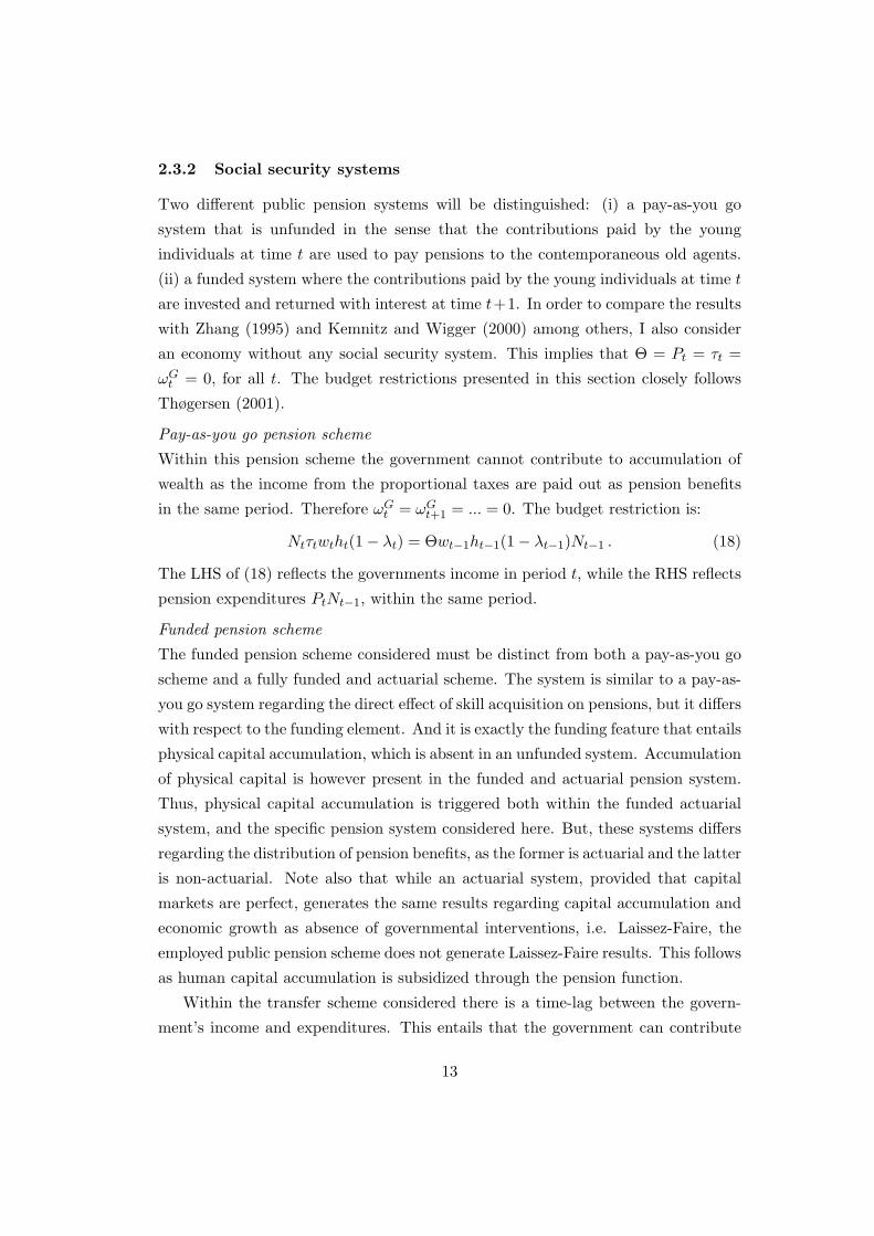
sion system. In this paper I will consider both one unfunded and one funded pension
scheme. Both systems contain subsidizing of education. The funded system are thus
7
not equivalent to absence of social security programs. As aforementioned I also con-
sider an economy without any governmental interference. Old-age consumption is
consequently:
c2,t+1 = Rt+1St + Pt+1 . (10)
The pension function I apply is closely related to the one used in Kemnitz and
Wigger (2000). Pension payments are positively linked to former wage and the level
of human capital for each individual. For analytical purposes I use the following
simple functional form:7
Pt = Θwt−1ht−1(1− λt−1) , (11)
where 0 < Θ < 1 denotes the constant pension ratio. Note that the pension func-
tion is non-actuarial in the sense that an increase in human capital affects pension
payments in two ways. First, investment in human capital affects pensions via the
effect on wage income, as human capital increases the wage per hour but also re-
duces the time spent on paid work. Second, investment in human capital is assumed
to have a direct positive effect on pensions apart from the effect via wage income.
This channel accounts for the intergenerational cross subsidy. This element of the
model ensures that the positive spillover of investments in human capital on the
productivity of future generations is captured.
Proposition 1 The effect of studytime on pension benefit is concave. If (1 −λt)−1 > ψ′(λt)/ψ(λt), the pension benefit is decreasing in studytime unambiguously.
If (1 − λt)−1 < ψ′(λt)/ψ(λt), the effect depends on the relative size of the terms in
∂Pt+1/∂λt.
Proof. Let wt = wt(ht). By inserting equation (5) into the pension function
and taking the partial derivative with respect to λt yields:
∂Pt+1
∂λt= Θ
w′t(·)ψ′(λt)ht−1ψ(λt)ht−1(1− λt)
+ wt(·)ht−1
[ψ′(λt)(1− λt)− ψ(λt)
],
which implies that:1
1− λt>ψ′(λt)ψ(λt)
⇒ ∂Pt+1
∂λt< 0 .
7The choice of functional form does not alter the qualitatively conclusions.
8
But, if ψ′(λt)/ψ(λt) > (1 − λt)−1, then ∂Pt+1/∂λt > (<) 0, if the second term is
greater (less) than the first term in the derivative.
Proposition 1 can intuitively be explained as follows. An increase in studytime
has two effects on pension benefits working in opposite directions. One effect is sim-
ply that an increase in studytime increases human capital,8 and thereby increases
pension payments. However, the wage rate is not necessarily increasing in study-
time,9 and as efficient wage is derived by multiplying the wage rate with human
capital, the outcome of this factor is ambiguous. The other effect is related to total
wage and working hours. An increase in studytime reduces time spent on labor
market activities and thereby reduces labor income. The result can therefore be
interpreted to imply that studytime increase pension benefits up to a certain point
(or certain age), and thereafter the relation is decreasing. If one chooses to devote
period 1 for studying only, the pension receipt is nil. But, as λt ∈ 〈0, 1〉, we can only
infer that if λt → 1 ⇒ Pt → 0 on the boundary.
As time spent on human capital accumulation is endogenously determined, it is
necessary to study the relationship between studytime and pension benefits, as well
as studytime and lifecycle income. That studytime is uniquely determined can be
shown by the first order condition of the utility function with respect to λt. However,
as the first order condition for lifecycle income with respect to λt, necessarily must
yield the same result, since there is no direct effect on utility of λt, it is sufficient to
study the latter. By substituting (10) into (9) we obtain the intertemporal budget
constraint:
c1,t +c2,t+1
Rt+1= (1− τt)htwt(1− λt) +
Pt+1
Rt+1.
By inserting the accumulation of human capital (5) and the pension function (11),
into the consolidated budget constraint we get the following expression for lifecycle
income:
Wt := ψ(λt)wtht−1(1− λt)(
1− τt +ΘRt+1
), (12)
where wt = wt(ht) and ht is given by (5). Differentiating (12) with respect to time
spent on human capital accumulation and set equal to zero yields the following:
∂Wt
∂λt= 0 ⇒ ψ′(λt) =
ψ(λt)wt
(1− λt)[wt + ψ(λt)w′t(ht)ht−1
] > 0 , (13)
8Cf. Equation (5) and Assumption 2.
9Cf. equation (8).
9
where the last inequality follows from Assumption 2. The inequality implies that
wt > |ψ(λt)w′t(ht)ht−1|. Equation (13) represents the tradeoff between studying
and working. It implicitly defines the optimal length of studytime that maximizes
lifecycle income. This relationship implies that the time spent on human capital
accumulation depends positively on pension benefits.
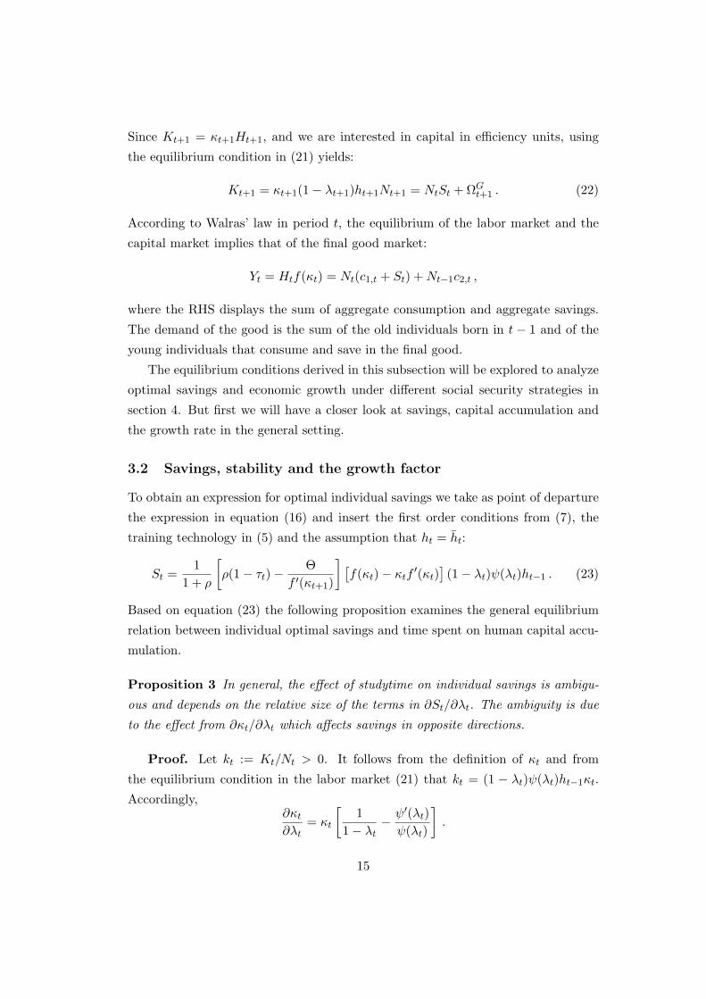
As we are interested in growth effects and capital accumulation we need an
expression for optimal individual savings. In order to illustrate the results I simplify
the model by using a logarithmic additive separable lifetime utility function:
u(c1,t, c2,t+1) = log c1,t + ρ log c2,t+1 , (14)
where ρ = 1/(1 + ξ) ∈ 〈0, 1〉 is the psychological discount factor, where ξ > 0
stands for the constant pure rate of time preference of an individual, which varies
inversely with ρ. It follows that the utility function u(·, ·) satisfies Assumption 3 and
has an intertemporal elasticity of substitution equal to 1. The consumption choice
and thereby optimal savings behavior is obtained by maximizing the lifetime utility
function (14) subject to the intertemporal budget constraint in (12). By combining
the two first order conditions for consumption we obtain the following intertemporal
Euler equation for consumption:
u′1(c1,t, c2,t+1)u′2(c1,t, c2,t+1)
= Rt+1 ⇒ c2,t+1 = ρRt+1c1,t . (15)
Inserting (9), (10) and the pension function (11) into the Euler equation (15) deter-
mines the optimal fraction saved as st = (1+ρ)−1[ρ(1− τt)−Θ(Rt+1)−1
]. Optimal
savings per individual young agent is therefore:
St =1
1 + ρ
[ρ(1− τt)−
ΘRt+1
]wtht(1− λt) . (16)
This expression demonstrates individual optimal savings, and implies the following
partial equilibrium effects.
Proposition 2 Private savings increases in the interest rate, given wages and con-
tributions. When the public pension ratio satisfies Θ < ρ(1−τt)Rt+1, private savings
increases in wages, given the interest rate and contributions. The effect of studytime
on individual savings is ambiguous and depends on the relation between ψ(λt) and
ψ′(λt)(1− λt), given the interest rate, wages and that Θ < ρ(1− τt)Rt+1.
10
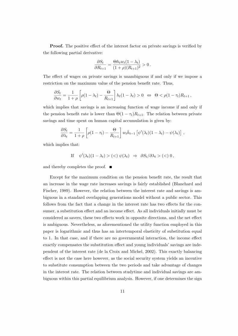
Proof. The positive effect of the interest factor on private savings is verified by
the following partial derivative:
∂St
∂Rt+1=
Θhtwt(1− λt)(1 + ρ)(Rt+1)2
> 0 .
The effect of wages on private savings is unambiguous if and only if we impose a
restriction on the maximum value of the pension benefit rate. Thus,
∂St
∂wt=
11 + ρ
[ρ(1− λt)−
ΘRt+1
]ht(1− λt) > 0 ⇔ Θ < ρ(1− τt)Rt+1 ,
which implies that savings is an increasing function of wage income if and only if
the pension benefit rate is lower than Θ(1 − τt)Rt+1. The relation between private
savings and time spent on human capital accumulation is given by:
∂St
∂λt=
11 + ρ
[ρ(1− τt)−
ΘRt+1
]wtht−1
[ψ′(λt)(1− λt)− ψ(λt)
],
which implies that:
If ψ′(λt)(1− λt) > (<) ψ(λt) ⇒ ∂St/∂λt > (<) 0 ,
and thereby completes the proof.
Except for the maximum condition on the pension benefit rate, the result that
an increase in the wage rate increases savings is fairly established (Blanchard and
Fischer, 1989). However, the relation between the interest rate and savings is am-
biguous in a standard overlapping generations model without a public sector. This
follows from the fact that a change in the interest rate has two effects for the con-
sumer, a substitution effect and an income effect. As all individuals initially must be
considered as savers, these two effects work in opposite directions, and the net effect
is ambiguous. Nevertheless, as aforementioned the utility function employed in this
paper is logarithmic and thus has an intertemporal elasticity of substitution equal
to 1. In that case, and if there are no governmental interaction, the income effect
exactly compensates the substitution effect and young individuals’ savings are inde-
pendent of the interest rate (de la Croix and Michel, 2002). This exactly balancing
effect is not the case here however, as the social security system yields an incentive
to substitute consumption between the two periods and take advantage of changes
in the interest rate. The relation between studytime and individual savings are am-
biguous within this partial equilibrium analysis. However, if one determines the sign
11
on (ψ′(λt)(1− λt)− ψ(λt)), the relation follows unambiguously. These implications
will not hold in general equilibrium, as will be explored in section 3.2.10
As the growth factor in this model is determined by both physical and human
capital accumulation, equation (16) will be fundamental in showing the dynamics
of capital in the economy. Before looking further at the growth factor let’s present
the set up of the public sector.
2.3 The public sector
2.3.1 National wealth
In this closed economy national wealth (Ωnt ) consists of a country’s human and
physical capital. This implies the definition, Ωnt := Kt + Ht. In this model it is
assumed that the capital stock consists of both capital owned by households and the
governments wealth (ΩGt ). The government can only accumulate wealth in form of
a pension fund that is built up from tax receipts from the young. This requires that
there exists a time-lag between the contributions of the young and the transfers to
the old agents. Human capital accumulation is assumed to only take place within
the private sector. This simplification is rationalized by the purely distributional
role of the government, and that human capital is owned by each individual. The
government’s wealth in the beginning of period t+1 can in general terms be expressed
as:
ΩGt+1 = RtΩG
t + τtwtht(1− λt)Nt −Θwt−1ht−1(1− λt−1)Nt−1 ,
where the second and the third term on the RHS is the government’s income from
taxes and payments to pensioners respectively. The growth factor presented in
this paper will be on per capita form. Accordingly, it is desirable to derive the
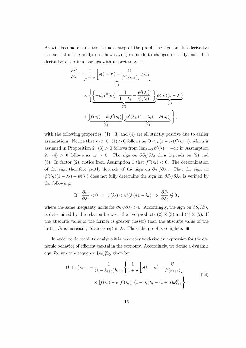
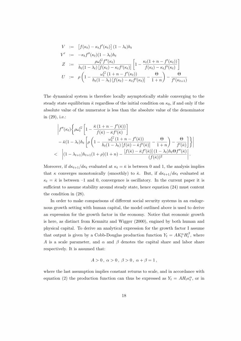
∣∣∣∣ .Moreover, if dκt+1/dκt evaluated at κt = κ is between 0 and 1, the analysis implies
that κ converges monotonically (smoothly) to κ. But, if dκt+1/dκt evaluated at
κt = κ is between –1 and 0, convergence is oscillatory. In the current paper it is
sufficient to assume stability around steady state, hence equation (24) must content
the condition in (28).
In order to make comparisons of different social security systems in an endoge-
nous growth setting with human capital, the model outlined above is used to derive
an expression for the growth factor in the economy. Notice that economic growth
is here, as distinct from Kemnitz and Wigger (2000), engined by both human and
physical capital. To derive an analytical expression for the growth factor I assume
that output is given by a Cobb-Douglas production function Yt = AKαt H
βt , where
A is a scale parameter, and α and β denotes the capital share and labor share
respectively. It is assumed that:
A > 0 , α > 0 , β > 0 , α+ β = 1 ,
where the last assumption implies constant returns to scale, and in accordance with
equation (2) the production function can thus be expressed as Yt = AHtκαt , or in
18
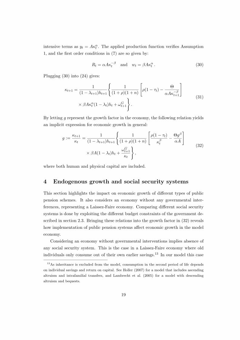
intensive terms as yt = Aκαt . The applied production function verifies Assumption
1, and the first order conditions in (7) are so given by:
Rt = αAκ−βt and wt = βAκα
t . (30)
Plugging (30) into (24) gives:
κt+1 =1
(1− λt+1)ht+1
1
(1 + ρ)(1 + n)
[ρ(1− τt)−
Θ
αAκ−βt+1
]
× βAκαt (1− λt)ht + ωG
t+1
.
(31)
By letting g represent the growth factor in the economy, the following relation yields
an implicit expression for economic growth in general:
g :=κt+1
κt=
1(1− λt+1)ht+1
1
(1 + ρ)(1 + n)
[ρ(1− τt)
κβt
− Θgβ
αA
]
× βA(1− λt)ht +ωG
t+1
κt
,
(32)
where both human and physical capital are included.
4 Endogenous growth and social security systems
This section highlights the impact on economic growth of different types of public
pension schemes. It also considers an economy without any governmental inter-
ferences, representing a Laissez-Faire economy. Comparing different social security
systems is done by exploiting the different budget constraints of the government de-
scribed in section 2.3. Bringing these relations into the growth factor in (32) reveals
how implementation of public pension systems affect economic growth in the model
economy.
Considering an economy without governmental interventions implies absence of
any social security system. This is the case in a Laissez-Faire economy where old
individuals only consume out of their own earlier savings.13 In our model this case
13As inheritance is excluded from the model, consumption in the second period of life depends
on individual savings and return on capital. See Holler (2007) for a model that includes ascending
altruism and intrafamilial transfers, and Lambrecht et al. (2005) for a model with descending
altruism and bequests.
19
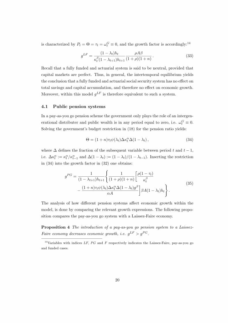
is characterized by Pt = Θ = τt = ωGt ≡ 0, and the growth factor is accordingly:14
gLF =(1− λt)ht
κβt (1− λt+1)ht+1
ρAβ
(1 + ρ)(1 + n). (33)
Recall that a fully funded and actuarial system is said to be neutral, provided that
capital markets are perfect. Thus, in general, the intertemporal equilibrium yields
the conclusion that a fully funded and actuarial social security system has no effect on
total savings and capital accumulation, and therefore no effect on economic growth.
Moreover, within this model gLF is therefore equivalent to such a system.
4.1 Public pension systems
In a pay-as-you go pension scheme the government only plays the role of an intergen-
erational distributer and public wealth is in any period equal to zero, i.e. ωGt ≡ 0.
Solving the government’s budget restriction in (18) for the pension ratio yields:
Θ = (1 + n)τtψ(λt)∆καt ∆(1− λt) , (34)
where ∆ defines the fraction of the subsequent variable between period t and t− 1,
i.e. ∆καt := κα
t /καt−1 and ∆(1− λt) := (1− λt)/(1− λt−1). Inserting the restriction
in (34) into the growth factor in (32) one obtains:
gPG =1
(1− λt+1)ht+1
1
(1 + ρ)(1 + n)
[ρ(1− τt)
κβt
− (1 + n)τtψ(λt)∆καt ∆(1− λt)gβ
αA
]βA(1− λt)ht
.
(35)
The analysis of how different pension systems affect economic growth within the
model, is done by comparing the relevant growth expressions. The following propo-
sition compares the pay-as-you go system with a Laissez-Faire economy.
Proposition 4 The introduction of a pay-as-you go pension system to a Laissez-
Faire economy decreases economic growth, i.e. gLF > gPG.
14Variables with indices LF, PG and F respectively indicates the Laissez-Faire, pay-as-you go
and funded cases.
20
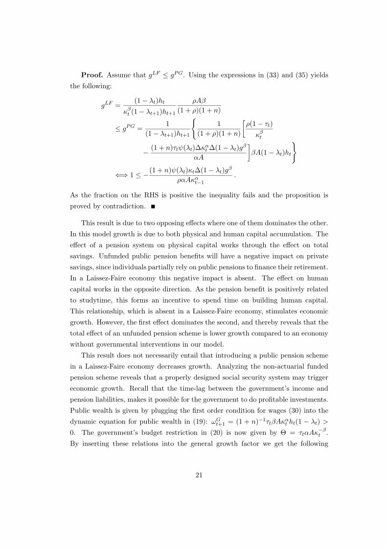
Proof. Assume that gLF ≤ gPG. Using the expressions in (33) and (35) yields
the following:
gLF =(1− λt)ht
κβt (1− λt+1)ht+1
ρAβ
(1 + ρ)(1 + n)
≤ gPG =1
(1− λt+1)ht+1
1
(1 + ρ)(1 + n)
[ρ(1− τt)
κβt
− (1 + n)τtψ(λt)∆καt ∆(1− λt)gβ
αA
]βA(1− λt)ht
⇐⇒ 1 ≤ −(1 + n)ψ(λt)κt∆(1− λt)gβ
ραAκαt−1
.
As the fraction on the RHS is positive the inequality fails and the proposition is
proved by contradiction.
This result is due to two opposing effects where one of them dominates the other.
In this model growth is due to both physical and human capital accumulation. The
effect of a pension system on physical capital works through the effect on total
savings. Unfunded public pension benefits will have a negative impact on private
savings, since individuals partially rely on public pensions to finance their retirement.
In a Laissez-Faire economy this negative impact is absent. The effect on human
capital works in the opposite direction. As the pension benefit is positively related
to studytime, this forms an incentive to spend time on building human capital.
This relationship, which is absent in a Laissez-Faire economy, stimulates economic
growth. However, the first effect dominates the second, and thereby reveals that the
total effect of an unfunded pension scheme is lower growth compared to an economy
without governmental interventions in our model.
This result does not necessarily entail that introducing a public pension scheme
in a Laissez-Faire economy decreases growth. Analyzing the non-actuarial funded
pension scheme reveals that a properly designed social security system may trigger
economic growth. Recall that the time-lag between the government’s income and
pension liabilities, makes it possible for the government to do profitable investments.
Public wealth is given by plugging the first order condition for wages (30) into the
dynamic equation for public wealth in (19): ωGt+1 = (1 + n)−1τtβAκ
αt ht(1 − λt) >
0. The government’s budget restriction in (20) is now given by Θ = τtαAκ−βt .
By inserting these relations into the general growth factor we get the following
21
expression:
gF =(1− λt)htβA
κβt (1− λt+1)ht+1
τt(1− gβ) + ρ
(1 + ρ)(1 + n). (36)
As showed in the next proposition, a funded pension scheme may increase growth if
the pension benefit is positively linked to the time spent on human capital accumu-
lation.
Proposition 5 Introducing a public funded pension system, that stimulates individ-
uals to build human capital in their first period of life, increases economic growth,
i.e. gF > gLF for gβ < 1.
Proof. Assume that gF ≤ gLF . Using the expression in (33) and (36) yields the
following:
gF =(1− λt)htβA
κβt (1− λt+1)ht+1
τt(1− gβ) + ρ
(1 + ρ)(1 + n)
≤ gLF =(1− λt)ht
κβt (1− λt+1)ht+1
ρAβ
(1 + ρ)(1 + n)
⇐⇒ τt(1− gβ) ≤ 0 ,
which proves the proposition by contradiction as τt(1− gβ) > 0 for gβ < 1.
This result is due to the link between skill acquisition in the first period of life,
and pension benefits in the second period of life, and that a funded scheme designed
in this way stimulates physical capital accumulation. In a Laissez-Faire economy,
physical capital accumulation is engined by private savings. These savings are re-
duced when a public social security system is implemented, but as a funded scheme
initiates accumulation of public wealth the effect on total savings in the economy is
absent. In the public funded system applied, these relations are maintained in addi-
tion to the relation between time spent on human capital accumulation and old-age
receipts. As the latter relation does not exist in a Laissez-Faire economy, growth is
stimulated by the introduction of such a properly designed public funded scheme.
Comparing the two social security systems reveals that growth is higher under
the funded program than with a pay-as-you go system, i.e. gF > gLF > gPG. The
main mechanism behind this result lies in the time-lag that follows with a funded
program. The government puts the tax receipts from the young to productive use
and gives rise to a positive rate of return. Consequently, even though both pension
schemes relates studytime and pension benefits, only the funded program stimulates
public investments.
22
5 Concluding remarks
In this paper I present an overlapping generations model with endogenous growth,
where both human and physical capital accumulation are the engines of output
growth. Moreover, human capital accumulation is assumed to spill over to the nest
generation and thus represent a positive externality on economic growth. The ap-
plied pension function explicitly takes account of this externality by relating skill
acquisition and pension benefits, as well as wages, human capital and pension ben-
efits. A similar pension function is used in Kemnitz and Wigger (2000). However,
they suppress all other relations but the one between pension benefits and time spent
on human capital formation. In their analysis, where human capital accumulation
is the engine of growth, it is shown that an unfunded social security system leads to
higher growth, compared to a Laissez-Faire economy. The conclusion is driven by
the pension function that stimulates human capital investment, a mechanism that
is absent in a Laissez-Faire economy. Zhang (1995) reaches the same conclusions
in a model where investment in human capital of children is the engine of endoge-
nous growth. The conclusion follows as unfunded social security reduce fertility and
increases human capital investment per child to per family income when private
intergenerational transfers are operative.
In contrast to these papers I find that a pay-as-you go pension system generates
lower growth than in a Laissez-Faire economy. This result is due to two opposing ef-
fects where the positive effect from higher saving in a Laissez-Faire economy, exceeds
the negative effect from lower human capital formation. The negative effect arises
as the link between pension benefits and time spent on skill acquisition is absent
in an economy without a social security system. However, this does not exclude
public pension as a growth promoting fiscal policy. The analysis in this paper finds
that a properly designed funded pension scheme that stimulates both physical and
human capital accumulation leads to higher economic growth than absence of social
security and governmental interference. Physical wealth is here accumulated by the
government as well as by private individuals. Formation of human capital is stim-
ulated by the pension system, due to the relation between studytime and pension
receipts.
23
References
Aghion, P. and Howitt, P. (1999), Endogenous Growth Theory. The MIT Press.
Arrow, K.J. (1962), The Economic Implications of Learning by Doing. Review of EconomicStudies 29, 155–173.
Azariadis, C. and Drazen, A. (1990), Treshold Externalities in Economic Development.Quarterly Journal of Economics 105, 501–526.
Belan, P., Michel, P. and Pestieau, P. (1998), Pareto-improving Social Security Reform withEndogenous Growth. The Geneva Papers on Risk and Insurance Theory 23, 119–125.
Blanchard, O.J. and Fischer, S. (1989), Lectures on Macroeconomics. The MIT Press.
Brauninger, M. and Vidal, J-P. (2000), Private versus public financing of education andendogenous growth. Journal of Population Economics 13, 387–401.
Cohen, D. and Soto, M. (2007), Growth and Human Capital – Good data, good results.Journal of Economic Growth 12, 51–76.
Coulombe, S., Tremblay, J-F. and Marchand, S. (2004), International Adult LiteracySurvey: Literacy scores, human capital and growth across fourteen OECD countries.Catalogue no. 89-552-MIE, Statistics Canada.
d’Autume, A. and Michel, P. (1994), Education et Croissance. Revue d’Economie Politique104, 457–499.
de la Croix, D. and Michel, P. (2002), A Theory of Economic Growth: Dynamics and Policyin Overlapping Generations. Cambridge University Press.
Diamond, P.A. (1965), National Debt in a Neoclassical Growth Model. American EconomicReview 55, 1126–1150.
Galor, O. (2007), Discrete Dynamical Systems. Springer.
Holler, J. (2007), Pension Systems and their Influence on Fertility and Growth. Universityof Vienna Working Paper NO.0704.
Kemnitz, A. and Wigger, B.U. (2000), Growth and Social Security: The Role of HumanCapital. European Journal of Political Economy 16, 673–683.
Lambrecht, S., Michel, P. and Vidal, J-P. (2005), Public Pensions and Growth. EuropeanEconomic Review 49, 1261–1281.
Lucas, R. E. (1988), On the Mechanics of Economic Development. Journal of MonetaryEconomics 22, 3–42.
24
Romer, P. (1986), Increasing Returns and Long-Run Growth. Journal of Political Economy94, 1002–1035.
Saint-Paul, G. (1992), Fiscal Policy in an Endogenous Growth Model. Quarterly Journal ofEconomics 107, 1243–1259.
Samuelson, P.A. (1958), An Exact Consumption Loan Model of Interest with or withoutThe Social Contrivance of Money. Journal of Political Economy 66, 467–482.
Thøgersen, Ø. (2001), Reforming Social Security: Assessing the effects of alternative fundingstrategies in a small open economy. Applied Economics 33, 1531–1540.
Wiedmer, T. (1996), Growth and Social Security. Journal of Institutional and TheoreticalEconomics 152, 531–539.
Zhang, J. (1995), Social Security and Endogenous Growth. Journal of Public Economics 58,185–213.
Zhang, J. (1996), Optimal Public Investment in Education and Endogenous Growth. Scan-dinavian Journal of Economics 98, 387–404.
25
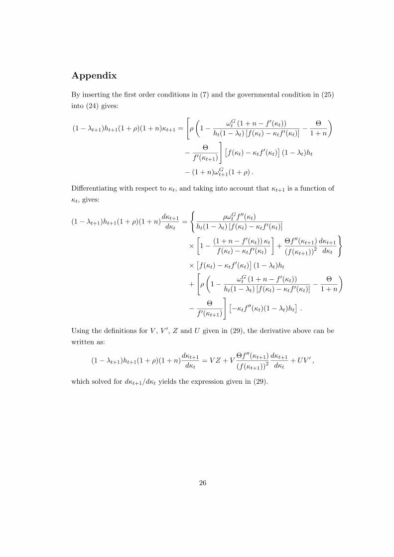
Appendix
By inserting the first order conditions in (7) and the governmental condition in (25)
into (24) gives:
(1− λt+1)ht+1(1 + ρ)(1 + n)κt+1 =
[ρ
(1− ωG
t (1 + n− f ′(κt))ht(1− λt) [f(κt)− κtf ′(κt)]
− Θ1 + n
)
− Θf ′(κt+1)
] [f(κt)− κtf
′(κt)](1− λt)ht
− (1 + n)ωGt+1(1 + ρ) .
Differentiating with respect to κt, and taking into account that κt+1 is a function of
κt, gives:
(1− λt+1)ht+1(1 + ρ)(1 + n)dκt+1
dκt=
ρωG
t f′′(κt)
ht(1− λt) [f(κt)− κtf ′(κt)]
×[1− (1 + n− f ′(κt))κt
f(κt)− κtf ′(κt)
]+
Θf ′′(κt+1)(f(κt+1))
2
dκt+1
dκt
×[f(κt)− κtf
′(κt)](1− λt)ht
+
[ρ
(1− ωG
t (1 + n− f ′(κt))ht(1− λt) [f(κt)− κtf ′(κt)]
− Θ1 + n
)
− Θf ′(κt+1)
] [−κtf
′′(κt)(1− λt)ht
].
Using the definitions for V , V ′, Z and U given in (29), the derivative above can be
written as:
(1− λt+1)ht+1(1 + ρ)(1 + n)dκt+1
dκt= V Z + V
Θf ′′(κt+1)(f(κt+1))
2
dκt+1
dκt+ UV ′ ,
which solved for dκt+1/dκt yields the expression given in (29).