Page 1
Human Computer Interface Using
Electroencephalography
by
Vamsi Krishna Manchala
A Thesis Presented in Partial Fulfillment of the Requirements for the Degree
Master of Science
Approved May 2015 by the
Graduate Supervisory Committee:
Sangram Redkar, Chair
Bradley Rogers Thomas Sugar
ARIZONA STATE UNIVERSITY
August 2015
Page 2
i
ABSTRACT
Brain Computer Interfaces are becoming the next generation controllers not only in
the medical devices for disabled individuals but also in the gaming and entertainment
industries. It is important to have robust and fail proof signal processing and machine
learning modules which operate on the raw EEG signals and estimate the current thought
of the user.
In this thesis, several techniques used to perform EEG signal pre-processing,
feature extraction and signal classification were discussed, validated and verified. To
further improve the performance unsupervised feature learning techniques were
investigated by pre-training the Deep Learning networks. Use of pre-training stacked
autoencoders have been proposed to solve the problems caused by random initialization of
weights in neural networks.
Motor Imagery (imaginary hand and leg movements) signals are acquire using the
Emotiv EEG headset. Different kinds of features have been extracted and supplied to the
machine learning (ML) stage, wherein, several ML techniques are applied and validated.
During the validation phase the performances of various techniques are compared and
some important observations are reported. Further, deep Learning techniques like
autoencoding have been used to perform unsupervised feature learning. The reliability of
the features is analyzed by performing classification by using the ML techniques
mentioned earlier. The performance of the neural networks has been further improved by
pre-training the network in an unsupervised fashion using stacked autoencoders and
supplying the stacked autoencoders’ network parameters as initial parameters to the neural
network. All the findings in this research, during each phase (pre-processing, feature
Page 3
ii
extraction, classification) are directly relevant and can be used by the BCI research
community for building motor imagery based BCI applications.
Additionally, this thesis attempts to develop, test, and compare the performance of
an alternative method for classifying human driving behavior. It proposes the use of driver
affective states to know the driving behavior. The purpose of this part of the thesis was to
classify the EEG data collected while driving simulated vehicle and compare the
classification results with those obtained by classifying the vehicle parameters. The
objective here is to see if the drivers’ mental state is reflected in his driving behavior.
Page 4
iii
DEDICATION
It is my genuine gratefulness and warmest regard that I dedicate this work to my
family and friends. A special feeling of gratitude to my mother whose love has filled my
heart with lots of positive energy and always motivated me to make her happy. My father
has always been a huge source of motivation and encouragement, his good examples have
taught me to work hard for the things that I aspire to achieve. I will always try to make him
proud. My brothers Jai and Mohan were always with me, in every walk of my life, always
loved me and whished for my success. My friend Shankar, who stood by me and tried to
make me a better individual, taught me and corrected my mistakes as an elder brother. He
became my family away from home. I miss you all.
Last but most importantly, I would like to dedicate this to God, for loving me and
blessing me with this life.
Page 5
iv
ACKNOWLEDGMENTS
I wish to express my sincere thanks to my supervisor, Prof. Sangram Redkar. This
thesis would not have been complete without his expert advice and unfailing patience. I
am also most grateful for his continuous help, support and advice (academic and personal)
throughout my Graduate study. I couldn’t have asked for and wouldn’t have got a better
advisor than him.
I would like to thank my committee members Dr. Bradley Rogers and Dr. Thomas
Sugar for serving on my committee.
Page 6
v
TABLE OF CONTENTS
Page
LIST OF TABLES .............................................................................................................. vi
LIST OF FIGURES ............................................................................................................ vii
CHAPTER
1 INTRODUCTION ................. ................................................................................. 1
1.1 Overview ..............................................................................................1
1.2 Understanding The Brain ......................................................................1
1.3 Electroencephalography ........................................................................5
1.4 Brain Computer Interface And Its Applications ....................................9
1.5 Learning To Control Brain Signals .....................................................11
2 BACKGROUND ................... ............................................................................... 13
2.1 Signals Used For Eeg Based Bci ........................................................13
2.2 EEG Signal Acquisition ......................................................................16
2.3 Signal Pre-Processing .........................................................................17
2.4 Data Decomposition............................................................................20
2.5 Feature Extraction ...............................................................................23
2.6 Classification/Machine Learning ........................................................30
2.7 Deep Learning.....................................................................................51
2.8 Tools Used In This Thesis...................................................................61
3 EXPERIMENTS, DATA ANALYSIS AND RESULTS ...................................... 72
3.1 Data Collection ...................................................................................72
3.2 Data Analysis ......................................................................................80
Page 7
vi
CHAPTER Page
3.3 Feature Extraction ...............................................................................85
3.4 Classification And Validation .............................................................90
3.5 Unsupervised Feature Learning& Deep Learning ...............................96
4 HUMAN EMOTION RECOGNITION WHILE DRIVING ................... ........... 101
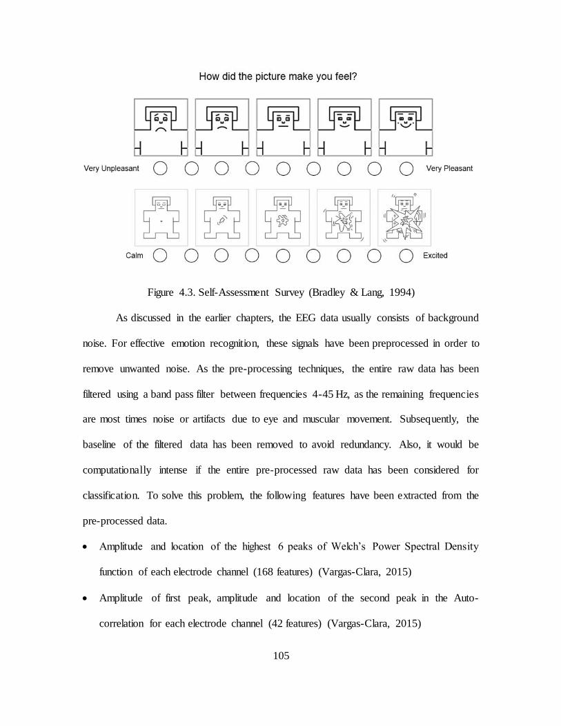
4.1 Introduction.......................................................................................101
4.2 Experimental Design.........................................................................103
4.3 Driving Behavior Classification using Participants’ EEG .................122
5 CONCLUSION ................... ............................................................................... 130
5.1 Summary And Conclusions...............................................................130
5.2 Future Work ......................................................................................132
REFERENCES....... ........................................................................................................ 133
APPENDIX
A IRB APPROVAL............................................................................................... 137
Page 8
vii
LIST OF TABLES
Table Page
1.1. Significance Of EEG In Different Frequency Bands ............................................ 7
2.1. Notations Used In Neural Networks. .................................................................. 50
2.2. Notations Used In Autoencoders. ....................................................................... 58
2.3. Emotiv EEG Headset Specifications................................................................... 68
3.1. Results Of The BCI Competition III, Dataset 3a................................................. 74
3.2. Classification Accuracies With KNN Method Using Different K Values ........... 91
3.3. Accuracies with KNN Method Using Different K Values on Data from Emotiv 91
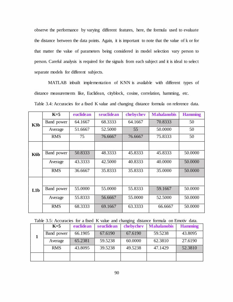
3.4. Accuracies for Fixed K Value and Changing Distance Formula, Standard Data 92
3.5. Accuracies for a Fixed K Value and Changing Distance Formula, Emotiv Data 93
3.6. SVM Classification Results for Different Kernel Functions, Standard Data ....... 94
3.7. SVM Classification Results for Different Kernel Functions, Data from Emotiv. 94
3.8. LDA Classification Results for Different Kernel Functions, Standard Data ....... 95
3.9. LDA Classification Results for Different Kernel Functions, Data from Emotiv . 95
3.10. Classification Results of NN with Different No. of Neurons, on Standard Data 99
3.11. Classification Results of NN with Different Hidden Neurons, on Emotiv Data . 99
3.12. Results Of SA+NN with Different Hidden Neurons, on Standard Data .......... 100
3.13. Results Of SA+NN with Different Hidden Neurons, on Emotiv Data ............ 100
3.14. Classifying Features Learned from Autoencoder Using KNN-Standard Data 102
3.15. Classifying Features Learned from Autoencoder Using KNN-Emotiv Data ... 102
3.16. Classifying Features Learned from Autoencoder Using KNN-Standard Data 102
3.17. Classifying Features Learned from Autoencoder Using KNN-Emotiv Data ... 102
Page 9
viii
Table Page
3.18. Classifying Features Learned from Autoencoder Using SVM-Standard Data 103
3.19. Classifying Features Learned from Autoencoder Using SVM-Emotiv Data ... 103
3.20. Classifying Features Learned from Autoencoder Using LDA-Standard Data . 103
3.21. Classifying Features Learned from Autoencoder Using LDA-Emotiv Data ... 103
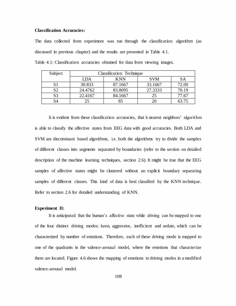
4.1. Classification Accuracies Obtained for Data from Viewing Images ................ 108
4.2. Driving Scenarios Descriptions........................................................................ 113
4.3. Classification Accuracies of Driving Parameters ............................................. 114
4.4. Results Using KNN, on Vehicle Parameters from Different Subjects.............. 115
4.5. Results Using DA, on Vehicle Parameters from Different Subjects................. 116
4.6. Results Using K- NN, on Vehicle Parameters from Different Subjects ........... 116
4.7. Results Using SA, on Vehicle Parameters from Different Subjects ................. 117
4.8. Results Using LDA, on EEG Data from Different Subjects............................. 119
4.9. Results Using KNN, on EEG Data from Different Subjects ............................ 120
4.10. Results Using SVM, on EEG Data from Different Subjects ............................ 120
4.11. Results Using SA, on EEG Data from Different Subjects ............................... 121
4.12. Results Using LDA, on EEG Data from Different Subjects ............................ 123
4.13. Results Using SVM, on EEG Data from Different Subjects ........................... 123
4.14. Results Using SVM, on EEG Data from Different Subjects ........................... 124
4.15. Results Using SA, on EEG Data from Different Subjects ............................... 124
4.16. Comparing Results with Different Classification Techniques for S1 ............... 126
4.17. Comparing Results with Different Classification Techniques for S2 ............... 126
4.18. Comparing Results with Different Classification Techniques for S3 ............... 127
Page 10
ix
Table Page
4.19. Comparing Results with Different Classification Techniques for S4 ............... 127
Page 11
x
LIST OF FIGURES
Figure Page
1.1. Cerebral Cortex ..................................................................................................... 3
1.2. Motor And Sensory Cortex ................................................................................... 4
1.3. Frequency Plots of EEG in Different Frequency Ranges ....................................... 6
1.4. 10-20 Standard Electrode Placement ..................................................................... 8
1.5. Physiological Signals Expected From Each Node of The 10-20 System ............... 8
2.1. Time Domain Behavior of P300 Signals. ............................................................. 14
2.2. Behavior of ERD For Left and Right Motor Imagery in Alpha Band................... 15
2.3. ICA Decomposition of EEG................................................................................. 22
2.4. Time Frequency Maps (Stft) of C3, C4 And Cz Electrodes in MI........................ 29
2.5. Showing the Changes in Bias and Variance Errors with Model Complexity........ 34
2.6. Typical Holdout Setup. ........................................................................................ 37
2.7. Typical Arrangement Showing the Random Subsampling Method...................... 38
2.8. Typical Setup Depicting the K-Fold Cross Validation Technique ........................ 39
2.9. Typical Setup Depicting the Leave-Out-One Cross Validation Technique. ......... 39
2.10. Showing the Typical Schema of K-NN. .............................................................. 40
2.11. LDA Hyper-Plane. .............................................................................................. 41
2.12. Hyper-Plane and Support Vectors. ...................................................................... 43
2.13. Before and After Increasing Dimensionality by Kernel Trick ............................ 44
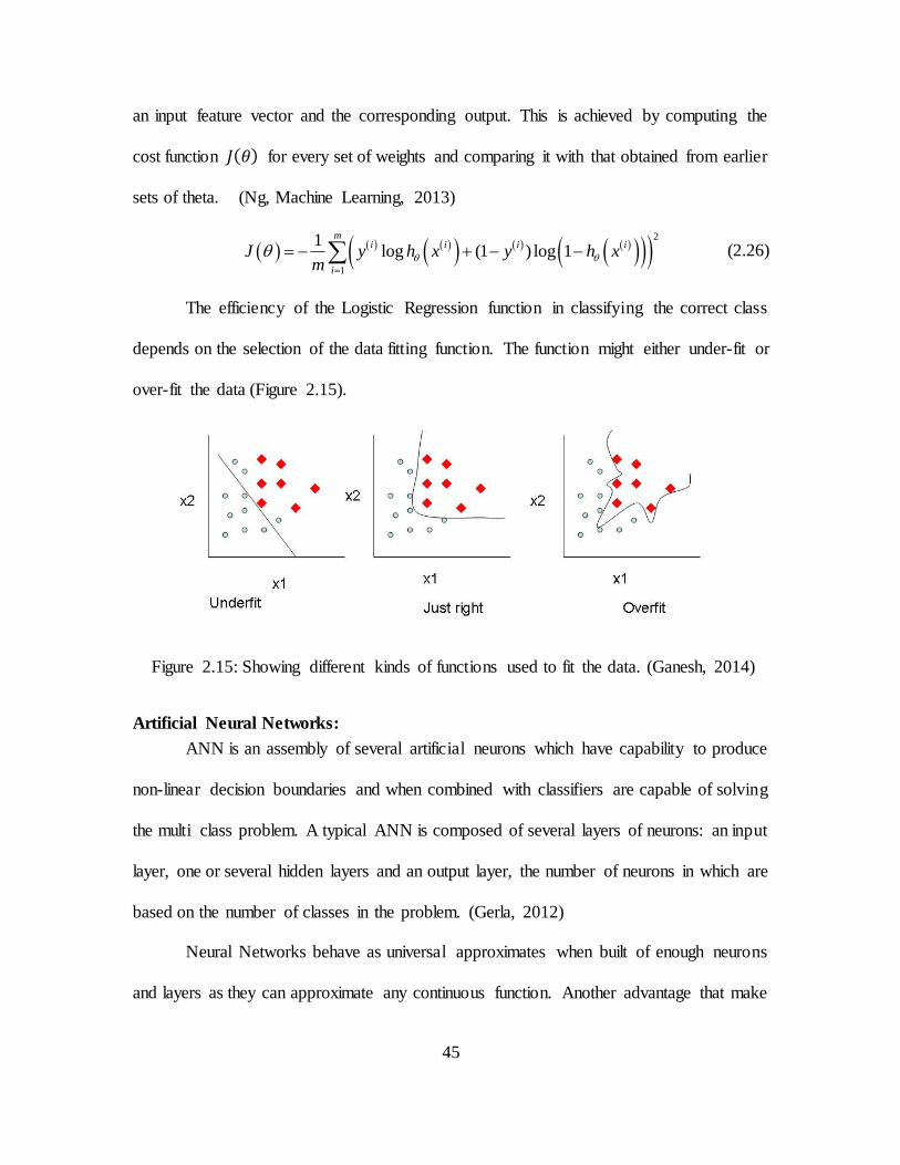
2.14. Logistic Function ................................................................................................. 45
2.15 Different Kinds of Functions Used to Fit the Data ............................................. 46
2.16. Single Neuron Used in a NN ............................................................................... 47
Page 12
xi
Figure Page
2.17. Typical Neural Network ...................................................................................... 48
2.18. NN With Input, Hidden and Output Layers for Multi-Class Classification ......... 50
2.19. Sparse Autoencoder Learning an Identity Function ............................................. 55
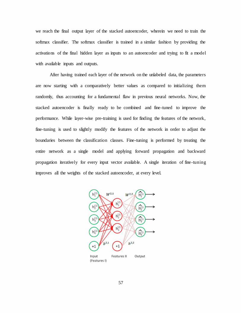
2.20. First Layer Autoencoder Module in The Stacked Autoencoder ........................... 57
2.21. Second Layer of Stacked Autoencoder ................................................................ 60
2.22. Training The Softmax Classifier ......................................................................... 60
2.23. Final Network of The Stacked Autoencoder ........................................................ 61
2.24. Core Modules of BCI in BCI2000 ....................................................................... 63
2.25. Bcilab Working Environment .............................................................................. 66
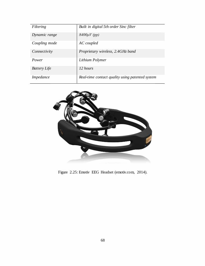
2.26. Emotiv EEG Headset .......................................................................................... 69
2.27. Electrode Locations in an Emotiv EEG Headset .................................................. 70
3.1. Timing of The Experimental Paradigm ............................................................... 74
3.2. Position of The Electrodes Used The Paradigm .................................................. 74
3.3. Stimulus Presentation Module in BCI2000 ......................................................... 77
3.4. Paradigm Created to Capture Data from Emotiv ................................................. 77
3.5. Showing Usual Electrode Placement Using Emotiv Headset .............................. 78
3.6. Showing the Electrode Placement Used in this Thesis to Acquire MI Data ........ 78
3.7. Frequency Plot of The C3, Cz And C4 Electrodes. (Subject: K3b) ..................... 80
3.8. Frequency Plot of The C3, Cz And C4 Electrodes. (Subject: K6b) ..................... 80
3.9. Frequency Plot of The C3, Cz And C4 Electrodes. (Subject: L1b) ...................... 81
3.10. Frequency Plot of All The 14 Electrodes of Emotiv Headset. (Subject: 1) ........... 82
3.11. Frequency Plot of All The 14 Electrodes of Emotiv Headset. (Subject: 2) ........... 82
Page 13
xii
Figure Page
3.12. Spectrogram Plot ................................................................................................. 83
3.13. 2R Plots Between Channel Number And Frequency ........................................... 84
3.14. Steps to Extract Band Power Features ................................................................. 86
3.15a. Alpha Band Power Plotted With C4 And C3 on 2d Xy Plane ............................. 87
3.15b. Beta Band Power Plotted With C4 And C3 on 2d Xy Plane................................ 87
3.16. 2d Plot of Average Values of C3, C4 Time Series. BlueRight, Red Left ... 88
3.17. 2d Plot of Root Mean Square of The Raw Signals On C3, C4 Of Each Trial ..... 89
3.18. Structure of The Neural Network Used ............................................................. 96
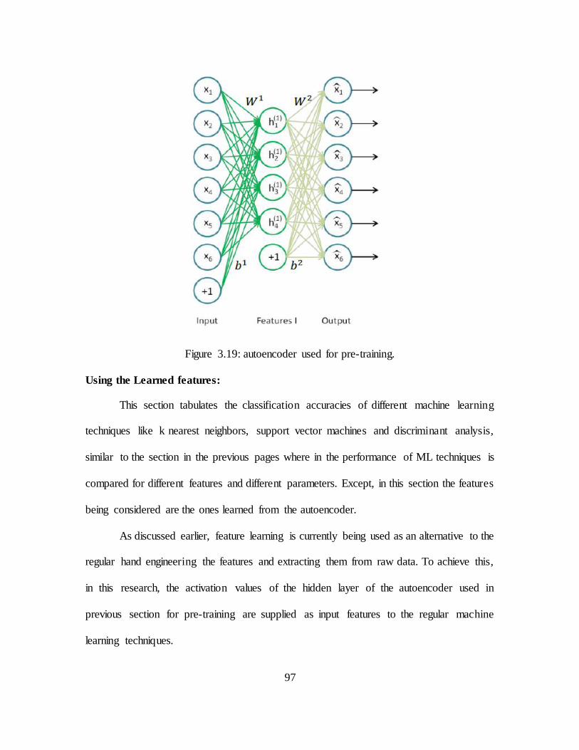
3.19. Autoencoder Used for Unsupervised Pre Training ............................................. 98
3.20. Autoencoder Used for Unsupervised Pre Training .......................................... 100
3.21. Obtaining Less Complex Features From The Pre-Trained Autoencoder .......... 100
4.1. Proposed Driving Behavior Classification Approach ....................................... 102
4.2. Valence-Arousal Model ................................................................................... 104
4.3. Self-Assessment Survey .................................................................................... 105
4.4. Differences Between IAPS Scores And Self-Assessments Scores .................... 107
4.5. Affective State Classification Based on Valence-Arousal Model ..................... 107
4.6. Mapping of Driving Mode to Affective States ................................................. 109
4.7. Rs-600 Driving Simulator ................................................................................. 111
4.8. Planned Driving Route ...................................................................................... 112
Page 14
1
CHAPTER 1
INTRODUCTION
1.1 OVERVIEW:
Recent advancements and discoveries in the areas of brain imaging and cognitive
neuroscience have enabled us to interact directly with the human brain. With the aid of
these technologies and sophisticated sensors, currently researchers are able to observe and
monitor the changing thought process in the form of low power electrical signals. These
signals are used to make brain-computer interfaces (BCIs) possible and develop
communication systems in which users explicitly manipulate their thought process, instead
of motor movements, to control computers or communication devices.
With the growing societal recognition for the difficulties faced by the people with
physical disabilities, BCIs are primarily aimed to develop systems that solve their
problems. The need for such systems is extremely high, mainly to those who suffer from
apocalyptic neuromuscular injuries and gradual neurodegenerative diseases, which
eventually slow down the user’s voluntary muscular activity while leaving the cognitive
functions intact. The current BCI research is also focused, like many other Human
Computer Interfaces, in the areas of Entertainment, Gaming, Consumer Electronics and
etc.
1.2 UNDERSTANDING THE BRAIN:
Acquiring the EEG Signals, accurately, is the first step involved in BCIs. It is
important to have a complete knowledge of the physiology and anatomy of human brain.
This would be helpful in identifying the correct locations of the sensory nodes and measure
the required signals.
Page 15
2
1.2.1 ARCHITECTURE OF THE BRAIN:
A typical human brain is made of approximately hundred billion nerve cells
(neurons), which have the amazing capability to collect and transmit electrochemica l
signals, over long distances, to other neurons. Brain, with the help of this network of
neurons, controls the mental and physical actions of a human body by passing on the
message signals throughout the body. The four major parts of the human brain are
Cerebrum, Diencephalon, Cerebellum and Brain stem.
The cerebrum, which is the uppermost and the largest portion of brain, is divided
into two hemispheres, right hemisphere and left hemisphere, and each hemisphere is further
divided into of four lobes (As shown in Figure 1.1)- Frontal lobe- which is often related to
planning, reasoning, problem solving, movements and emotions; Parietal lobe- which is
associated to orientation, recognition, movement, perception of stimuli, etc., Occipital
lobe- which is located at the very back of the head is mainly associated to visual processing;
Temporal lobe- which is involved in pattern matching, memory, speech and language
processing. In spite of the similarities in their physical structure, both the hemispheres are
very different in their functionalities. For instance, right brain is correlated to the expressive
and creative tasks like Recognizing faces, Expressing Emotions, Reading emotions, etc.
and left brain is correlated to actions like Logic, Critical thinking, reasoning. Also, most
motor and sensory signals travelling to and from the brain cross the hemispheres, which
means that the right brain senses and controls the left side of the body and vice versa.
1.2.2 SENSORY MOTOR CORTEX:
The somatosensory cortex of the brain is the part of the brain that receives and
processes the sensory inputs from all other parts of the body. And, the motor cortex is the
Page 16
3
part of the human brain that controls and acts as an input to the voluntary muscles. The
motor cortex controls the body responses according to messages from the surrounding
environment. The motor nerves twine through muscle fibers like a root system that ends in
clusters called motor end plates. These fibers start muscle contractions by means of
chemical messengers. As shown in Figure 1.2, the motor area is divided between the two
sides of the brain, called hemispheres, which are different in size, shape and the roles they
play. The right hemisphere controls the motor responses of the left side of the body, and
left hemisphere controls the right side.
Figure 1.1: A diagram of the cerebral cortex, with various lobes specialized for
performing different functions. (Stangor C. , 2012)
Page 17
4
Figure 1.2: Illustrating the Motor and Sensory cortex regions of left hemisphere of the
brain. (Stangor C. , 2012)
Page 18
5
1.3 ELECTROENCEPHALOGRAPHY:
Electroencephalography refers to the phenomenon of recording the electrical
activity along the scalp and Electroencephalogram (EEG) is referred to the recorded signals
and is the measure of voltage fluctuations/variations occurred due to the flow of
electrochemical currents in the neurons of the brain. During the signal recording procedure,
electrodes consisting of small metal discs are pasted over the scalp. To maintain proper
connectivity with the actual electrical signals, these electrodes are made wet by a
conducting jell or liquid. However, the BCI world is now seeing some commercial dry
EEG headsets which would serve the purpose of capturing the data and transferring to the
Computer through wireless medium. Patterns of the EEG signals, detected by the
electrodes, represent that there is continuous activity present in the human brain and the
varying intensities of the signal are determined by the changing mental and physical states
of the body. These intensities of the EEG Signals recorded over the surface of the brain
range from 0 microvolts to 200 microvolts.
The rhythmic activity of the brain signals is often divided to different bands on
terms of frequency. Although these frequency bands are a matter of nomenclature, these
designations are usually used to imply the fact that the rhythmic activity in a certain
frequency range is observed due to certain biological significance and are often noted to
have certain distribution over the scalp. Figure 1.3 shows the different frequency bands the
EEG data is divided into, and Table 1.1 shows the significance of these frequency bands
and related cognitive tasks these bands correspond to.
Page 19
6
Figure 1.3: Frequency Plots of EEG in different Frequency Ranges. (Ortiz, 2012)
Page 20
7
Table 1.1: Significance of EEG in different frequency bands.
Type Frequency (Hz) Location Use
Delta up to 4 Everywhere occur during sleep, coma
Theta 4 – 7 Hz temporal and parietal correlated with emotional stress
(frustration & disappointment)
Alpha 8 – 12 Hz occipital and parietal reduce amplitude with sensory stimulation or mental imagery
Beta 12 – 30 Hz parietal and frontal can increase amplitude during
intense mental activity
Mu 9-11 Hz frontal (motor cortex) diminishes with movement or
intention of movement
1.3.1 EEG ELECTRODE PLACEMENT:
10-20 system is an internationally accepted and practiced scheme of electrode
placement on the human scalp. The 10 and 20 in the name refer to the percentage distance
of nodes from each other in proportion to the head size. The electrode locations suggeste d
by this method belong to locations on cerebral cortex and the letters F, T, C, P and O denote
the frontal, temporal, central, parietal and occipital respectively. Except for the central
location the remaining are all lobes of the brain. The numbers indicate the position of the
node on the scalp, even number denote right side of the head, odd number denote the left
side and Z indicates that the node is located on the central line of the head. Figure 1.4
illustrates these standard electrode positions and Figure 1.5 illustrated the kind of
physiological signals to expect from these individual nodes.
Page 21
8
Figure 1.4: Standard electrode positions and placement on the human scalp.
(EEG_Measurement_Setup, n.d.)
Figure 1.5: Showing the physiological signals expected from each node of the 10-20
system. (John, 2014)
Page 22
9
1.4 BRAIN COMPUTER INTERFACE AND ITS APPLICATIONS:
Brain Computer Interface (BCI) is a branch of Human Computer Interface which
involves obtaining the brain signals, corresponding to specific form of thoughts, and
translating them to machine commands. It is a communication system which performs the
transfer of messages or commands by the means of human thoughts and not conventiona lly
by peripheral nerves and muscles.
The research communities initially focused on developing applications using the
BCI technology for assistive devices, keeping in mind the needs of physically challenged
individuals. However, the need for BCI and awareness has increases to a large extent that
there are a numerous, multifaceted and non-medical, areas in which the researchers are
currently exploring the possible applications of BCIs. Some of the currently existing
technologies and applications of BCI are categorized into following-
1.4.1 APPLICATIONS OF BCI:
USER STATE MONITORING:
A highly anticipated application amongst the BCI communities is that the future
user-communication systems would require a parallel feedback of the user mental state or
intentions along with his physical state. For example, it is important for the automobile to
react to the user’s drowsiness. These future applications are called system-symbiosis or
effective computing and require the systems to gather details regarding mental states like
emotions, attention, workload, stress, fatigue, etc. and interpret them. (Erp, Lotte, &
Tangermann, 2012)
Page 23
10
EVALUATION:
Online and/or offline evaluation of applications using the physiological data might
lead to several conclusions regarding the users state and help in comparing different use
cases. For instance, a recent research on analyzing the brain imaging results of cell phone
use during driving has proved that even hands free and voice activated use of mobile phone
is as dangerous as drunken driving. Another recent research in this EEG data evaluation
has been conducted by Arizona State University, which focuses to find out how to
leverage social media to improve educational and training environments. The goal of this
research was to analyze the EEG data captured from students while they were using
Facebook and try make a record of what they were looking at and also their affected state,
and ultimately forward their findings to use in online learning communities and make
online learning more interesting for the students. (ANGLE’s Facebook project, 2013)
GAMING AND ENTERTAINMENT:
The gaming industry is earning most of its market share by making use of the
wearable technology. Particularly, over the past few years, new game have been developed
based on the commercially available EEG headsets by the companies like NeuroSky,
Emotiv, Uncle Milton, Mattel and MindGames. The usual gaming experience has been
enhanced and enriched by the use of BCIs in the gaming industry. For example, a typical
BCI based game would no longer be controlled by the keyboard but would function based
on the mental states, immersion, flow, surprise, frustration etc.; of the player. (Erp, Lotte,
& Tangermann, 2012)
Page 24
11
DEVICE CONTROL:
Brain Computer Interfaces are already being used in controlling many devices like
motorized wheel chairs, prosthetic limbs, simulate muscular movement, controlling home
appliances, lights, room temperature, television, operating doors, etc. The need for Brain
Computer Interfaces in the embedded market is being explored, recent advances in BCI
have seen projects using off the shelf EEG headsets and embedded single board computers
like Beagle Bone Black and Raspberry Pi. (Erp, Lotte, & Tangermann, 2012)
1.5 LEARNING TO CONTROL BRAIN SIGNALS:
A typical BCI falls into two categories, dependent and independent. Dependent
BCIs do not use the brains conventional output pathways to transfer the message to the
external world, but activity in these pathways is needed to generate the brain activit ies,
which could be used for BCI. In contrast, an independent BCI does not depend on the brains
conventional output pathways, in any way. Consider an example matrix of letters that flash
one at a time. In a dependent BCI, the brains output channel is EEG signal which is depends
on gaze direction of the eye. However, in an independent BCI, the user selects a specific
letter by producing a P300 evoked potential when the letter flashes, the EEG signal is
dependent on the user’s intent. (Tan & Nijholt, 2010)
In order to operate the BCIs successfully, the user is required to develop and
maintain a new skill, a skill to properly control the specific electrophysiological signals
depending on the kind of response expected; and it also requires that the BCI translate that
control into machine commands that accomplish the user’s intent related to that particular
thought signal. Meaning, the users need to learn and practice the skill to intentiona lly
manipulate their brain signals. (Tan & Nijholt, 2010) To date, there have been two
Page 25
12
approaches for training users to control their brain signals. In the first, users are given
specific cognitive tasks such as motor imagery to generate measurable brain activity. Using
this technique the user can send a binary signal to the computer, for example, by imagining
sequences of rest and physical activity such as moving their arms or doing high kicks. The
second approach, called operant conditioning, provides users with continuous feedback as
they try to control the interface (Tan & Nijholt, 2010). Users may think about anything (or
nothing) so long as they achieve the desired outcome. Over many sessions, users acquire
control of the interface without being consciously aware of how they are performing the
task. Unfortunately, many users find this technique hard to master (Tan & Nijholt, 2010).
Page 26
13
CHAPTER 2
BACKGROUND
2.1 SIGNALS USED FOR EEG BASED BCI:
EEG activity can be obtained and processed in the time domain or in spatial domain
or both, which can be used to initiate an EEG based communication. Also, it is evident
from the above discussion that, on proper training and practice, users can control the
features of electrophysiological signals as and when required. Hence the use of EEG
signals is widely in practice amongst the BCI researchers. The current days BCIs aim at
identifying the brain activity that might be translated into machine commands. A numbe r
of signal patterns have been studied and some of them have been reported as easily
identifiable as well as easy to control for the user. These signals can be divided into two
main categories: (Vaughana, et al., 2002)
Visual Evoked Potentials (VEP):- They refer to the electrical potentials yielded
in the brain as a result to the external visual stimuli like light. These recordings of the
Visual Evoked Potentials are made from the scalp above visual cortex and are used to
determine the direction of eye gaze. Hence, these signals depend on the user’s ability to
control the eye gaze direction. For example, these signals are currently being used in
applications which intend to generate motor output in robots with the aid of the users gaze
direction. (Vaughana, et al., 2002)
Slow Cortical Potentials: - Slow voltage fluctuations generated in cortex are
considered to be the lowest frequency components of the EEG recorded over the scalp.
These potential shifts which occur over 0.5 –10.0 s are called slow cortical potentials
(SCPs). Negative SCPs are typically associated with movement and other functions
Page 27
14
involving cortical activation, while positive SCPs are usually associated with reduced
cortical activation. (Vaughana, et al., 2002)
P300 potentials: - A positive peak at about 300 ms would evoke over the parietal
cortex when a sporadic or particularly significant visual, auditory, or somatosensory stimuli
is combined and/or interspersed with frequent or routine stimuli. This is called P300 which
is a positive peak around 300ms after the target stimulation onset and occurs at the parietal
lobe. A P300 based BCI requires no training to generate the signals. Figure 2.1 shows the
onset of P300 signal 300ms after the stimulus.
Figure 2.1: showing the behavior of P300 signals. (Vaughana, et al., 2002)
N400 potentials: - The N400 is an event-related potential (ERP) component which
is evoked by unexpected linguistic stimuli. It is characterized as a negative deflection
(topologically distributed over central-parietal sites on the scalp), peaking approximate ly
400ms (300-500ms) after the presentation of the stimulus. (Vaughana, et al., 2002)
Page 28
15
Event related desynchronization/synchronization (ERD/ERS): - Visible change
that occur in the mu (8 -13 Hz) and beta (13 – 30 Hz) bands while performing or imagining
the motor task is known as Event related desynchronization. Event related synchroniza t ion
is a phenomenon in which the power increases in the mu and beta bands when the subjects
stops motor imagery. ERD/ERS are observed to have different spatial characteristics and
powers for different limbs. For example, if the subjects imagines a left hand movement,
ERD/ERS is observed in right hemisphere with good strength and left hemisphere with
poor strength (Pfurtscheller & Neuper, 1997). Figure 2.2 shows the Event related de-
synchronization and synchronization during right and left hand motor imagery.
Figure 2.2: showing the behavior of ERD for left and right motor imagery in Alpha band.
(Pfurtscheller & Neuper, 1997)
2.2 EEG SIGNAL ACQUISITION:
As discussed in the earlier sections of this thesis, electroencephalogram (EEG) is a
recording of the bio-potentials from the surface of the scalp. More specifically, these
recordings are the electrochemical potentials measured from the neurons at the cerebrum
Page 29
16
of the human brain. Since these signals are recorded from the surface of the scalp, it is most
likely that potentials from many cells are being measured at the same time. At first glance,
EEG data may look like an unstructured, non-stationary, noisy signal. However, advanced
signal processing techniques can be used to separate different components of the brain
waves. These separate components can then be associated with different brain areas and
functions.
The potentials acquired from a single neuron are very less than the desired levels.
However, the final electrical potential recorded at a single sensor node is large enough, to
carry out the further signal processing steps, since the signal captured at a single electrode
is a summation of either synchronous or asynchronous signals originated at various neurons
in the vicinity. This phenomenon would not cause any problems because, it is evident from
the brain topologies that all the neurons located in a vicinity would fire for all the mental/
physical activities which are specific for the location.
In order to carry on with the signal acquisition stage, it is important to identify
whether the BCI signals are going to be dependent or independent; have evoked or
spontaneous inputs. In addition to these, it is also important to decide on which method to
adopt in obtaining the signals; a non -invasive or an invasive. Needles to mention, there is
no specific reason why a BCI could not combine invasive and non- invasive methods, or
evoked and spontaneous inputs. Ultimately, in the signal acquisition stage, the signals are
obtained from the electrodes, amplified, digitized and made available for the further stages.
Page 30
17
2.3 SIGNAL PRE-PROCESSING:
It is always possible that the acquired EEG data is combined with a lot of artifacts
due to the electrical activity of eyes (EOG: Electroocculogram) or muscles (EMG:
Electromyogram). The best way to avoid these unwanted components is to maintain ideal
conditions during the signal acquisition, like maintaining a relaxed position which would
involve minimum or no physical movements. However, on a practical note, maintaining
such laboratory conditions in everyday BCIs is not realizable and such systems when used
outdoors to operate embedded applications like UGV or Wheelchair, is not considered to
be robust and reliable. This problem can generally be solved by adopting effective pre-
processing techniques which are responsible to clean the signal from unwanted artifacts
and/or enhance the information embedded in these signals.
It is observed that the amplitude of these muscle artifacts is much higher than the
usual EEG signals and during most offline analysis these can be removed by visual
inspection. But to eliminate these artifacts in a more effective manner it is important to
apply various spatio-spectro-temporal filtering techniques.
2.3.1 TEMPORAL FILTERS:
As discussed earlier, the EEG signals can be divided into several frequency ranges
and this division plays an important role in the EEG research as each frequency range is
connected to a specific cognitive action. For example, the delta (0.5-4 Hz) is obtained
during sleep and mu (8-13 Hz) are related to motor imagery.
Temporal filters such as low-pass or band-pass filters are used to separate the frequency
components which are connected to the physiological action under consideration and
restrict the analysis to the signals in that range. For example, the motor imagery signals
Page 31
18
produce a significant amount of variance in the 8-30 Hz frequency range, which contains
both the mu and beta rhythms. Hence, for signal processing in the motor imagery related
applications, usually the mu and beta rhythms are extracted. Such a temporal filtering can
be achieved by using Discrete Fourier Transform (DFT) or using Finite Impulse Response
(FIR) or Infinite Impulse Response (IIR) filters.
1. Discrete Fourier Transform filtering: DFT is generally used to represent the time
domain signal in frequency domain as a linear combination of different frequencies (f).
Thus, the DFT 𝑆(𝑓) of a signal 𝑠(𝑛) is acquired from N time domain samples and can be
defined as shown in equation (2.1):
21
0
i fnN
N
n
S f s n e
(2.1)
Hence, filtering a signal using DFT means setting the coefficients of the frequency
components, which do not belong to the frequency ranges in hand, to 0. And, evaluate the
inverse transform of 𝑆(𝑓) to get back the filtered signal, as shown in equation (2.2).
21
0
i nkN
N
n
s n S k e
(2.2)
2. Filtering with Finite Impulse Response filters: FIR filters are considered to be the
linear filters which determine the filtered signal 𝑦(𝑛) by making use of the M last samples
of a raw signal 𝑠(𝑛), shown in equation (2.3):
0
M
k
k
y n a s n k
(2.3)
Page 32
19
3. Filtering with Infinite Impulse Response filters: As FIR filters, IIR filters are linear
filters. However they are recursive filters which make use of the outputs of the P last filter
values along with the M last input samples as shown in equation (2.4):
0 1
pM
k
k k
y n a s n k by n k
(2.4)
2.3.2 SPECIAL FILTERS:
Similar to the temporal filters, various spatial filters are used to isolate the desired
features from the EEG Signals and discard the irrelevant data. For example, each channel
of a typical EEG headset designed according to the universal 10/20 method of electrode
placement is designated for a specific physiological actions (C3 is responsible to give out
the signals related to right hand motor imagery and C4 is responsible to give out the signals
related to left hand motor imagery). (Lotte F. , 2008)One most widely used spatial filter ing
technique is to capture the signal from a single electrode which transmits signal related a
particular physiological action of interest, avoiding the signals from surrounding electrodes
which probably might contain noise and some redundant data.
For example, in a Motor Imagery application signals from electrode locations C3
and C4 are considered for the entire processing because it is known that these nodes are
located on the sensorimotor cortex area. Similarly, for the BCIs based on SSVEP
applications, the most considered electrodes are the O1 and O2 electrodes as they are
located over the visual cortex.
However, it is important to capture information from few neighboring electrodes as
they might contain relevant information related to the physiological task in hand. But there
are a few potential problems that might arise due to the consideration of more number of
Page 33
20
nodes, like redundancies, correlations between channels, more number of features and
hence the need for more training data. Typically spatial filters are used to obtain new
signals free of redundant data by defining linear combination of the original signals. Few
of the most widely used spatial filters are: (Lotte F. , 2008)
Bipolar filters - Filter output is obtained as a result of difference between two adjacent
electrodes.
3 3 3C FC CP (2.5)
Average reference filter - The outputs of all channels are summed and averaged, and this
averaged signal is used for further processing in the BCI.
1
1 k
k i
i
C Ck
(2.6)
Laplacian filter - The filtered signal represents the difference between an electrode and a
weighted average of the surrounding electrodes.
3 3 3 5 1 34*C C FC C C CP (2.7)
2.4 DATA DECOMPOSITION USING COMPONENT ANALYSIS:
The Blind source separation (BSS) techniques are considered to be one of the most
effective ways of estimate and remove only the nuisance signal related to specific source
of noise or for that matter any unwanted data. A number of techniques have been proposed
under the tag of ‘blind source separation’ and mainly function to estimate specific sources
of EEG signal assuming that the observed signal can be understood as a mixture of origina l
source signals.
Page 34
21
Most data decomposition methods are based on the assumption that the origina l
source signals are uncorrelated and hence aim to decompose the observed signal into a
number of uncorrelated components. Independent Component Analysis is probably one of
the best known methods which belong to the BSS family and solves the “cocktail party
problem” effectively. In a cocktail party problem, the measured signals which are recorded
from various sensor nodes is a result of unknown linear mixing of several sources, as shown
below.
m As (2.8)
Here, m is the matrix of measurements, with a sensor per row and a time sample
per column; s is a source matrix, with source per row and time sample per column and A
is considered be the mixing matrix. The main aim of BSS is to evaluate and estimate of s
without knowing A by finding an unmixing matrix W, which decomposes or linear ly
unmixes the multichannel EEG data into set of temporally independent and spatially fixed
components.
S Wm (2.9)
Independent Component Analysis is proved to be useful and effective in EEG
signal processing and BCI implementations. An ICA would un-mix the signals origina t ing
from different regions of the brain. In this way it probably become much easier to retain
the signals acquired from the regions of interest and discard components that are very likely
to be noise or artifacts. Then the EEG signals can be reconstructed using only the selected
components. Figure 2.3 shows the mechanism of ICA source separation in EEG signal
processing.
Page 35
22
Figure 2.3: ICA Decomposition of EEG. (Removing Artifacts from EEG, n.d.)
Common Spatial Patterns:
Common Spatial Patterns is another spatial filtering method which is one of the
most widely used ones in BCI research. According to this method, the EEG data is
decomposed into spatial patterns, the selection of which is made to maximize the variance
between the classes involved, as the data is projected onto these patterns. Hence, the
classification of the data during the test stage is made easy.
2.5 FEATURE EXTRACTION:
The BCI researchers are trying their hands on with the low-power embedded single
board computers like Beagle Board, Intel Galileo, Raspberry Pi and etc. These hardware
devices are efficient and perform well in most situations. However, signal acquisitions for
a typical EEG headset would lead in a huge amount of data since the acquisition might
Page 36
23
involve signals from number of electrodes ranging from 1 to 256 and the frequencies with
which the sampling is performed ranges from 100 Hz to 1000 Hz. These large amount of
data would prove to be computationally intensive and it might take a lot of time to classify
the test signals if the entire data is being used in the BCI. So, it is important to have
dimensionality reduction of the signals for Embedded BCI applications. Along with
dimensionality reduction, it is also important to have proper technique of identifying the
differences in the signals which belong to different classes because different physiologica l
actions might produce different signal pattern, the differences of which are not always
observable by inspection and also by applying classifying techniques on the origina l
signals.
Feature extraction is phenomenon of building a feature vector of features which are
considered to a small amount of data, derived from the main signals and, which best defines
the signal of interest and reflects the similarities and differences between signals of same
and different classes respectively.
Identifying and extracting relevant features is one of the most important steps in a
BCI as it is proved to be crucial for an effective classification stage. If the features extracted
from EEG are not relevant to the corresponding neurophysiological action, it would be very
difficult for the BCI to classify the training signals into their respective classes and hence
the system would not be performing effectively during the test phase. Thus, even if
applying classification steps on the raw signals might give results, it would be a slow
process and it is recommended to use an effective feature extraction technique in order to
maximize the speed and efficiency of the BCI.
Page 37
24
A number of basic measurements can be performed on the EEG data to extract
required information, while transformations can be used to view the signal for different
perspective. Below are some of the features that can be extracted from an EEG data and
investigated for performance during classification.
2.5.1 TIME SERIES:
Time series signal amplitude:
It has been earlier discussed that different physiological task would produce
different signal patterns in the EEG waveform. This fact can act as the basis of feature
extraction and hence the time series signal amplitudes from different electrodes can be used
as features and concatenated, probably after nominal preprocessing to remove noise, into
a feature vector and be used for classification of wave patterns belonging to different
classes’ physiological actions. However, this methodology of using the time series
amplitudes as features could prove to be computationally intensive for Real Time
Embedded systems applications, as they involve processing of huge amount of data, as
mentioned above, to alleviate the effect researchers generally make use of few spatial filters
or under-sampling the signals.
Signal Average Value:
Average value is one of the most straightforward measurement in an EEG signal.
To determine the average value of a time series, simple add the values of samples acquired
and divide by the number of samples.
1
1
N
avg k
K
x x xN
(2.10)
Page 38
25
Root Mean Squared (RMS):
Although the signal average is a basic measurement of the signal, it does not
provide any information regarding the variability of the signal. However, root-mean-
squared (RMS) value is a measurement that provides details regarding the signa l’s
variability and its average. RMS is obtained by first squaring the signal, then computing
its average and finally evaluating the square root of its average.
1/2
2
0
1 N
rms k
k
x xN
(2.11)
Variance:
The variance of a signal is a measure of its variability regardless of its average. In
statistics, variance is considered to be the measure of how far a set of numbers are spread
out. If the variance is 0, the numbers are all equal to mean (average), a lower variance
would imply that the values are closer to the mean and to each other and a higher variance
indicates the signals are spread out around the mean and from themselves.
2 2
1
1 ( )
1
N
k
k
x xN
(2.12)
Standard Deviation:
The standard deviation is another measure of a signal’s variability and is obtained
by computing the square root of the variance.
1/2
2
1
1 ( )
1
N
k
k
x xN
(2.13)
Page 39
26
Autoregressive components:
According to the Autoregressive methods, the time series signal 𝑋(𝑡) measured at
time t, can be represented as a weighted sum of the samples of the same signal from
previous timestamps added to noise 𝑁𝑡 which is generally Gaussian white noise.
1 21 2 k tX t a X t a X t a X t k N (2.14)
In most BCI applications based on AR components, it is assumed that different
physiological actions can be classified and differentiated based on the AR parameters. For
a multi-channel BCI system, the AR coefficients from different channels can be evaluated
and concatenated to form a feature vector, which can be used for the classification stage of
the BCI. However, the accuracy during the classification stages is considered to be directly
proportional to number of previous samples used to denote the current sample, as using
more samples would provide a more accurate estimate of the AR model. Here, there is
tradeoff between the required computational resources and accuracy of the system.
Hjorth parameters:
Evaluating the Hjorth parameters for the EEG signals is one of the effective ways
to indicate the statistical properties of the signal in the time domain. The three kinds of
parameters which are known as Hjorth parameters are Activity, Mobility and Complexity.
Activity: The variance of time function indicates the surface of the power spectrum in
frequency domain. The Activity value of a particular signal is large or small depending on
many /few high frequency components.
Activity X t VAR X t (2.15)
Page 40
27
Mobility: Is the square root of the ratio of the variance of the first derivative of the signal
and that of the signal. This parameter is proportionate to the standard deviation of the power
spectrum.
dX tActicity
dtMobility X t
Activity X t
(2.16)
Complexity: Evaluates how similar is the signal compared to pure sine wave. The value
of complexity would tend to 1 as the shape of the signal gets more similar to a pure sine
wave.
dX tMobility
dtComplexity
Mobility X t
(2.17)
2.5.2 FREQUENCY METHODS:
Band power features:
Extracting the band power features of an EEG signal is to filter the signal in a given
frequency band, squaring the filtered signal and finally averaging the squared values over
a given time window. Most times log-transformation is applied on these values so as to
have features with a distribution similar to normal distribution.
Power spectral density features.
Power spectral density features of the signal are simply the spectral distribution of
the signal, which gives information of the power of the signal in different frequencies. PSD
is often computed by squaring the Fourier Transform of the signal or by computing the
Fourier transform of the autocorrelation function of the signal.
Page 41
28
Time frequency representation:
The neurophysiological signals used in BCI research typically consist significant
amount of changes in frequency domain with changing time. For example, while collecting
the EEG data for 10s in a motor imagery experiment, the subject might be asked to perform
the actual imagery task only between 4 7s so the frequency domain representation of the
entire signal would definitely differ with timing information. Short-time Fourier transform
and wavelets are few most widely used Time frequency representation methods. The main
advantage of these methods is that they capture the relatively sudden temporal variations
of the signal and projecting those changes in the frequency domain.
Short-time Fourier transform: Short-time Fourier transform (STFT) simply multip lies
the input signal by a suitable windowing function w which is non-zero only over a short
period of time and then computes the Fourier transform of this windowed signal. The
discrete time STFT 𝑋(𝑛, 𝜔) of signal 𝑥(𝑛) is:
, j n
n
X n x n w n e
(2.18)
The main drawback of the STFT method is that it uses a window of fixed size and
leads to similar frequential and temporal resolution in all frequency bands. The
representation would be more informative if there were high temporal resolution for parts
of the signal with high frequencies. Wavelet analysis serves this purpose exactly.
Page 42
29
Figure 2.4: Time frequency maps (STFT) of C3, C4 and Cz electrodes for left and right
hand motor imagery. (Mu, Xiao, & Hu, 2009)
Considering the Figure 2.4 it is evident that the energy distributions on electrodes
C3, C4 and Cz are different and is differentiable is case of left and right hand motor imagery
at different points in time.
Wavelets: Wavelet transform, like Fourier transform, makes use of a basis functions and
decomposes the input signal. These basis functions are a set of wavelets 𝛷𝑎,𝑏 which are
scaled and translated versions of the mother wavelet 𝛷.
,
1a b
t bt
aa
(2.19)
The wavelet transform 𝑊𝑥 (𝑠, 𝑢) of a signal x can be written as:
,,x u sW s u x t t dt
(2.20)
Page 43
30
Here, s and u are respectively the scaling and translating factor. Wavelet transforms
possess the ability to analyze the signal at different scales simultaneously, this is one
advantage of WT over STFT. Signals at high frequencies are analyzed by high temporal
resolution, whereas the signals with low frequencies are analyzed by frequential resolution.
2.6 FEATURE TRANSLATION/ CLASSIFICATION:
2.6.1 MACHINE LEARNING:
Machine Learning is a sub-branch and a combination of Computer Science and
Artificial Intelligence. It is referred to as study and development of systems that can learn
from data and behave based on the gained knowledge, rather than explicit programming.
Applications of Machine Learning are currently growing exponentially with the need for
intelligent systems and understanding huge amounts of data being generated from various
sources and industries. It is particularly used instead of explicit rule-based programming
enabling the software to make decisions automatically based on the previous knowledge.
Some potential areas of research with Machine Learning include spam filtering, computer
vision, weather forecast and etc.
Classifier, being considered as a subset of Machine Learning, is one of the most
important part of a BCI system, it is responsible to classify the extracted features, from the
training data sets, into finite number of classes and thereby classify the test signals based
on different physiological tasks performed and help the BCI system make decisions and
translate them into machine commands. In an Embedded BCI system, it is very important
for the classification stage to be efficient and fast as the machine commands are expected
to be spontaneous and occur real time.
Page 44
31
A typical classification stage will require a training database, of selected features
and corresponding labels of individual signals, to train the classifier and this trained
information would be used in the future when a new signal is encountered and needs to be
classified into different classes and translated into machine commands. In this section, we
produce a brief introduce to different classification categories and few important
techniques per category.
In this section, we introduce to some of the important standards to be followed
during designing a ML system to classify data which enable us to understand and improve
the behavior and performance of the system. We first introduce basic idea of supervised
learning, unsupervised learning and reinforcement learning, later briefly explain the
Machine Learning techniques used and analyzed in this thesis. Then, different problems
like bias, variance have been explained along with their comparisons made using standard
data sets. Finally, the importance of cross-validation is explained. All the above mentioned
methods and verifications have been used on standard EEG data sets and on Motor Imagery
data recorded from Emotive Headset and results have been tabulated/graphica l ly
represented in the future chapters.
2.6.2 TYPES OF MACHINE LEARNING ALGORITHMS:
Supervised learning: It is one of the most widely used learning techniques to map
data to output value-often referred to as regression where the output variable takes
continues values or classify data into different classes-called as classification where a class
label is assigned to the output. Supervised learning is often used on EEG data to classify
them in to different physiological classes for example into Left or Right hand imagery task.
In order to successfully classify the test EEG data, supervised learning techniques require
Page 45
32
the user to provide with training data which consists of features obtained from single trials
and class labels corresponding to respective trials. The ultimate goal of a supervised
learning technique is to develop a model based the features and their responses provided
in the form of training data and classify the features of the test data into correct
responses/classes.
Unsupervised Learning: Unsupervised learning algorithms try to find hidden
structures and patterns in unlabeled data. In an unsupervised learning scenario, the system
is provided with simple sequence of inputs 1, 2, ..x x but is provided neither supervised
target outputs nor feedback from the environment. The representations made by the system
from the provided input data are used for decision making, effectively communicating the
scenario to another machines, predicting future inputs, etc. Two simple examples of
unsupervised learning are clustering and dimensionality reduction.
Reinforcement Learning: In reinforcement learning the machine interacts with its
surrounding environment by producing actions 1, 2, 3, ..a a a which effect the current
state of the environment, thereby results in the machine receiving some information. The
ultimate goal of the reinforcement learning system is to learn to behave in a way it
improvises the data which it receives over its lifetime.
2.6.3 BIAS- VARIANCE TRADEOFF:
Often times, if a learning algorithm does not behave as desired it is most likely due
to the high bias or high variance problem in the system. High bias is occurred due to under
fitting of the algorithm. The bias error of the system is attributed to its inability to
appropriately choose the function f, to estimate labels y of an input feature vector, from all
Page 46
33
the possible set of mapping functions. On the other hand, a high variance problem is caused
due to over fitting of the mapping function. This might reduce the performance of the
system when provided with new testing data. (Kakade & McAllester, Statistical Decision
Theory, Least Squares, and Bias Variance Tradeoff, 2006)
The Classification Mean Square Error can be decomposed in terms of bias and
variance (Kakade & McAllester, Statistical Decision Theory, Least Squares, and Bias
Variance Tradeoff, 2006).
2*
2* * *
22 2* * *
22
MSE
E y f x
E y f x f x E f x E f x f x
E y f x E f x E f x E E f x f x
Noise Biasf x Var f x
(2.21)
The first term is the noise square also called as output variance, on which users do not
usually have control. The second term is the variance of the mapping function, determining
how the prediction varies from average prediction (Kakade & McAllester, Statistica l
Decision Theory, Least Squares, and Bias Variance Tradeoff, 2006). The final term is the
bias squared, which determines the difference between the average prediction and the true
conditional mean.
Page 47
34
Figure 2.5: Showing the changes in bias and variance errors with model complexity.
(Fortmann-Roe, 2012)
According to the above equation, it is evident that to attain lowest classifica t ion
error it is important to have both variance and bias to be low. Unfortunately, there is a
tradeoff between bias and variance in most of the Machine Learning systems as the bias is
inversely proportional to the complexity of the model and variance is proportional to it.
Most stable classifiers tend to have a high bias and low variance, whereas the unstable
classifiers have a low bias and a high variance. This is the reason why sometimes the
simpler models perform better than the complex ones.
2.6.4 CROSS-VALIDATION:
Along with bias and variance problems, it is also important to understand the
significance of using cross-validation in the selection procedure of a Machine Learning
model, to validate the experimental results. Validation techniques are motivated by two
fundamental and most important problems in Machine Learning: Model Selection and
Performance Estimation.
Page 48
35
Model Selection:
Almost always, the performance of pattern recognition and the classifica t ion
techniques depends on single/multiple parameters. For instance, enlisted below are some
of the parameters used for model selection in different classification techniques (Rai,
2011).
Nonlinear Regression: Polynomials with different degrees.
K-Nearest Neighbors: Different choice of K.
Decision Trees: Different choices of number of levels.
SVM: Different choices of the misclassification penalty hyper parameter C.
Regularized Models: Different choices of the regularization parameter.
Kernel based Methods: Different choices of kernels.
Performance Estimation:
Once the model is chosen it is important to estimate its performance, which is
typically measured by evaluating the true error rate- the classifiers error rate on the entire
data set. (Rai, 2011)
A not so successful practice in Machine Learning techniques is using all the
available data to train the model and testing the trained model on the same data. This way
we will be able to observe just the bias error and not the variance error. From the Figure
2.5, it is evident that the bias error is inversely proportional to the complexity of the model
(for example: a higher order model or more number of variables). So, it is a good practice
to increase the complexity of the model and try to introduce some variance error while
reducing the bias error and thereby optimizing the system by lowering the training error.
But, there would not be any guarantee that the learned model would perform better when
Page 49
36
provided with a new test data. Here, arrives the need for validation data which is different
from training data and testing data. Validation data is used in selecting the right model by
validating the performance of different trained models.
The Holdout method:
According to the Holdout method, the entire data is split into two parts, Training
set, which is used to train the classifier and Validation set, used to estimate the error rate
of the trained classifier. Though the holdout method offers fairly good validation, it has a
few drawbacks because the total available dataset is not always large enough to be divided
into parts, also as the data samples acquired in the typical EEG experiments are single trial
data, the holdout estimate of error rate would be misleading if the validation data consisted
of failed single trials. Figure 2.6 shows the typical scenario of holdout cross validat ion
method.
Figure 2.6: Typical Holdout setup. (Lecture Notes- Pattern Recognition, 2013)
Random Subsampling:
In the random subsampling method, a fixed number of random samples are picked
from the entire dataset and used for validation while the remaining data samples are used
for training the model (shown in Figure 2.7). This process is performed K times, each with
a different random validation set and a validation error is recorded every time. The true
error estimate is obtained as the average of the errors obtained in each of the K iteration. A
Page 50
37
model with the smallest average validation error is chosen to be the optimal one. (Lecture
Notes- Pattern Recognition, 2013)
1
1
K
i
i
E eK
(2.22)
Figure 2.7: Typical arrangement showing the Random subsampling method. (Lecture
Notes- Pattern Recognition, 2013)
K-Fold Cross-Validation:
K -Fold cross validation is a method which is widely used amongst the ML
researchers to accurately validate the classifiers with the limited amount of available data.
According to this method it is suggested to equally divide the total data into k different sets
(Lecture Notes- Pattern Recognition, 2013). All the k different sets would be used to
validate the classifier in k different stages while using the remaining k-1 sets of data for
training (Shown in Figure 2.8). Finally overall performance of the classifier is calculated
by averaging the validation results obtained in all the stages.
1
1
K
i
i
E eK
(2.23)
The selection of the number of folds a K-Fold Cross Validation method needs to be
operated is still an unknown question. With a large number of folds, the bias of the error
Page 51
38
rate estimator would be small but the variance is usually high and also making the system
computationally intensive. However, with a small number of folds, the computation time
is reduced besides a small variance of the error rate estimator, but the bias will be large. In
practice, the choice of K is made based on the size of the dataset.
Leave-one-out Cross Validation:
Leave-one-out Cross Validation technique is same as the K-Fold Cross Validation
technique, wherein the value of K is chosen to be equal to the total number of samples in
the dataset. (Lecture Notes- Pattern Recognition, 2013). As shown in Figure 2.9, number
of experiments equal to the number of samples, where one sample is selected to be test case
in every experiment.
Figure 2.8: Typical setup depicting the K-Fold Cross Validation technique. (Lecture
Notes- Pattern Recognition, 2013)
Page 52
39
Figure 2.9: Typical setup depicting the Leave-out-one Cross Validation technique.
(Lecture Notes- Pattern Recognition, 2013)
2.6.5 MACHINE LEARNING/CLASSIFICATION TECHNIQUES:
k- Nearest Neighbor Classifier:
k- Nearest Neighbor (k-NN) is simple and effective classifier. The classifier
compares the test data with the training data. It evaluates the distances of each vector in
the training data form the test vector, finds k nearest neighbors around the test sample and
assigns the class label which is found amongst majority of the k nearest neighbors. The
bias of the k-NN algorithm is very low since it is deciding based on the nearby points.
However, it has a very high variance.
Some of the distance functions used in the k-NN algorithm are Eauclidean,
Standardized Euclidean, City block, Chebychev, Cosine distance, Manhattan, Minkowski,
Hamming, correlation distance, etc. Figure 2.10 shows region consisting of the test sample
and its nearest neighbors.
Page 53
40
Figure 2.10: Showing the typical schema of K-NN. (Tulsa, 2013)
Linear Discriminant Analysis:
The working principle of LDA is to make use of a hyper-plane which separates the
signals belonging to different classes. In a two-class problem, the two classes are separated
by a hyper-plane and the signals belonging to different classes are on either sides of the
hyper-plane. Similar to a two-class problem, different signals belonging to different classes
in a multi-class problem are separated by multiple hyper-planes. (Lotte F. , 2008)
Figure 2.11: LDA hyper-plane (Lotte F. , 2008)
Page 54
41
LDA generally assumes a normal distribution of the data with same covariance
matrices for all the signals. Each hyper-plane separating one class from the other classes is
obtained by evaluation the projection that maximizes the distance between the mean of one
class from the means of all other classes and minimizes the interclass covariance. Figure
2.11 shows the separating plane between two classes.
The main advantages of this method is that it has a very low computational requirements
and complexities, which makes it suitable for real time embedded applications. However
the main drawback of this method is that it would not work effectively on non-linear
complex EEG data.
Support Vector Machines (SVM):
Like LDA, SVM is also used to classify signals into different classes and identify
them when required, with the aid of a hyper-plane. However, SVM tries to solve the
problem of non-linear complex signals. In SVM, the selection of the hyper-plane is made
to maximize the width of the band which separates the nearest training points to increase
the generalization capabilities. (Gerla, 2012) (Lotte F. , 2008)
The hyper-plane, also called as decision border, segments the feature space into
parts equal to the number of classes of the signals. The result of the classification stage
would depends on which part of the plane is the test signal located. Figure 2.12 shows the
optimal hyper-plane separating two planes in SVM.
Page 55
42
Figure 2.12: Hyper-plane and support vectors. (LOTTE, 2008)
Depending upon whether or not the time series signals is linearly separable, the
SVM method would be able to convert the data into linearly separable and create nonlinear
decision boundaries to classify them (Figure 2.13). This phenomenon of building non-
linear decision boundaries is not much complex as is making the use of a kernel trick to
implicitly map the data to another space of higher dimensionality, where the data is linear ly
separable and the regular linear classifiers are still applicable. The kernel generally used in
BCI research is the Gaussian kernel:
2
2,
2
x yK x y exp
(2.27)
Page 56
43
Figure 2.13: Before and after increasing dimensionality by kernel trick. (Thornton,
2014)
Naïve Bayes classifier:
The Naïve Bayes classification algorithm is also used to classify the data into
different classes. It computes the probability with which a test sample with features
1 2, 3 ..,, ,mx x x x can belong to a particular class c1. Probabilities are evaluated for all the
classes and the test sample would be assigned a class, which it can belong to, with highest
probability. (Gerla, 2012)
Naïve Bayes probability function is as follows-
1
1 2
1 1
|| , , .. .,
|
m
l i lil m N m
q i qq i
p c p x cp c x x x
p c p x c
(2.28)
Where N is the total number of classes. The individual probabilities on the right-
hand side of the equation are evaluated from the training data (Gerla, 2012).
Page 57
44
Logistic regression used for Classification:
Unlike in the regression problem, the output values y of the model take a limited
number of discrete values in the classification problem. For example in a binary
classification the output y might either take a value of 1 or 0 depending on whether or not
the input feature vector belongs to the desired class? (Ng, Machine Learning, 2013) For
logistic regression used for classification, a sigmoid function is used as a hypothesis to
predict the output class as the output of a sigmoid would range between 0 and 1. Vectors
which produce output lower than 0.5 would be assigned a 0 class and the ones with an
output value more than 0.5 would be assigned a 1, as shown in Figure 2.14. (Ng, Machine
Learning, 2013)
1
1T
T
xh x g x
e
(2.24)
( )( ) 1/ (1 )zg z e (2.25)
Here, 𝑔(𝑧) is called the logistic function or the sigmoid function and 𝜃𝑖 ′𝑠 are the parameters
(also called as weights) parameterizing the space of logistic function mapping X and Y.
Figure 2.14: Showing the logistic function. (Ng, Machine Learning, 2013)
The main focus of the logistic regression classifier is to evaluate the values of the
weights 𝜃𝑖, in an iterative fashion, so as to reduce the difference between the hypothesis of
Page 58
45
an input feature vector and the corresponding output. This is achieved by computing the
cost function 𝐽(𝜃) for every set of weights and comparing it with that obtained from earlier
sets of theta. (Ng, Machine Learning, 2013)
2
1
1log (1 ) log 1
mi i i i
i
J y h x y h xm
(2.26)
The efficiency of the Logistic Regression function in classifying the correct class
depends on the selection of the data fitting function. The function might either under-fit or
over-fit the data (Figure 2.15).
Figure 2.15: Showing different kinds of functions used to fit the data. (Ganesh, 2014)
Artificial Neural Networks:
ANN is an assembly of several artificial neurons which have capability to produce
non-linear decision boundaries and when combined with classifiers are capable of solving
the multi class problem. A typical ANN is composed of several layers of neurons: an input
layer, one or several hidden layers and an output layer, the number of neurons in which are
based on the number of classes in the problem. (Gerla, 2012)
Neural Networks behave as universal approximates when built of enough neurons
and layers as they can approximate any continuous function. Another advantage that make
Page 59
46
the Neural Networks flexible for a great number of problems is that they can classify any
number of classes.
The intuition for Neural Networks can be built over the understanding developed
on Logistic Regression, in the previous section. Consider a supervised learning problem,
provided with labeled training data , x i y i . Neural Networks give a way of defining
a complex, non-linear form of hypotheses ,W bh x , with parameters , W b that we can fit
to our data.
Figure 2.16: Single Neuron used in a NN. (Ng, CS294A Lecture notes, 2011)
A single neuron (Figure 2.16) is a basic computational unit in a complex NN, takes
inputs 1, 2, 3......x x x and outputs 3
1
, ) ( ( )T
W b
i
i ih x W x f xf W b
, where
: f R R is called the activation function. Most cases it is either a sigmoid function or
a tanh function.
( )( ) 1/ (1 )zf z e (2.27)
( ) ( )z z
z zf
e ez tanh z
e e
(2.28)
Page 60
47
A Neural Network is built by connecting multiple simple neurons together to form
a complex network. (Ng, CS294A Lecture notes, 2011)For example, Figure 2.17 shows a
NN which is built with one input layer, one hidden layer and an output layer, capable of
classifying two different actions.
Figure 2.17: Typical NN. (Ng, CS294A Lecture notes, 2011)
The computation that neural network in Figure 2.17 represents is given by:
(2) (1) (1) (1) (1)
1 11 1 12 2 13 3 1
(2) (1) (1) (1) (1)
2 21 1 22 2 23 3 2
(2) (1) (1) (1) (1)
1 31 1 32 2 33 3 3
(3) (2) (2) (2) (2) (2) (2) (2)
, 1 11 1 12 2 13 3 1
( )
( )
( )
( ) ( )w b
a f W x W x W x b
a f W x W x W x b
a f W x W x W x b
h x a f W a W a W a b
(2.29)
Suppose we have a fixed training set (1) (1) ( ) ( ){( , y ),......( , y )}m mx x of m training
examples. For a single training example ( , )x y , we define cost function as-
Page 61
48
2
,
1( , ; , ) ( ) y
2W bJ W b x y h x (2.30)
And for a training set of m samples, the overall cost function would be-
1 1( ) ( ) ( ) 2
1 1 1 1
1 12
( ) ( ) ( ) 2
,
1 1 1 1
1( , ) ( , ; , ) ( )
2
1 1( ) y ( )
2 2
l l l
l l l
n s smi i l
ji
i l i j
n s smi i l
W b ji
i l i j
J W b J W b x y Wm
h x Wm
(2.31)
The first term in the above equation is an average sum-of-squares error term. The second
term is a regularization term (also called a weight decay term) that tends to decrease the
magnitude of the weights, and helps prevent over fitting. (Ng, CS294A Lecture notes,
2011) The ultimate goal in the Neural Networks is to come up with the best set of
parameters (1) (1) (2) (2)(W ,b , W ,b ), W b , which would minimize the ( , )J W b . To train
the network, we will initialize each parameter ( )l
ijW and each ( )l
ib to random non-zero
values, and update the ( )l
ijW and ( )l
ib for every iteration by applying techniques like gradient
descent. One iteration of gradient decent updated the parameters as follows:
( ) ( )
( )
( ) ( )
( )
: ( , )
: ( , )
l l
ij ij l
ij
l l
i i l
i
W W J W bW
b b J W bb
(2.32)
Table 2.1: Notations used in Neural Networks. (i) (i)( , y )x i th Training example
, ( )w bh x Output of hypothesis on input x , using parameters ,W b .
( )l
ijW The parameter associated with the connection between unit j in
layer l , and unit i in layer 1l .
( )l
ib The bias term associated with unit i in layer 1l .
Page 62
49
( )l
ia Activation of unit i in layer l of the network.
Figure 2.18: Neural Network showing input, hidden and output layers for multi-class
classification. (Ng, CS294A Lecture notes, 2011)
2.7 Deep Learning:
Feature Extraction discussed in section 2.3 has a lot of features that are successfully
being used in the BCI research. Many of the features are discovered by observation of raw
data by many researchers, over several years. The area of feature extraction is considered
to be almost saturated and the researchers are seeing themselves getting interested to
explore more sophisticated and automated feature extraction techniques. Deep Learning is
one area currently being explored by the Machine Learning research communities to
emulate the feature learning and classification mechanism taking place in the human brain
to understand the information it gets from different natural sensors, by breaking down the
Page 63
50
complex information into new and simple representations. One potential use of Deep
Learning is unsupervised feature learning, which tries to understand the complex data and
represent it in much less complexity.
It is a class of Machine Learning techniques that exploit many layers of non-linear
information, used to model complex relations among data, by being able to represent the
data in multiple levels. Often used for supervised or unsupervised feature extraction and
transformation, and for pattern analysis and classification.
“A sub-field of machine learning that is based on learning several levels of
representations, corresponding to a hierarchy of features or factors or concepts, where
higher-level concepts are defined from lower-level ones, and the same lower- level
concepts can help to define many higher-level concepts. Deep learning is part of a broader
family of machine learning methods based on learning representations. An observation
(e.g., an image) can be represented in many ways (e.g., a vector of pixels), but some
representations make it easier to learn tasks of interest (e.g., is this the image of a human
face?) from examples, and research in this area attempts to define what makes better
representations and how to learn them.” (Deep Learning, 2015)
Deep Learning refers to a rather wide class of machine learning techniques and
architecture. Based on how the architecture has been designed and its intended use, Deep
Learning techniques can be classified into three major areas.
Deep networks for unsupervised or generative learning: Used to capture high-
order correlation of the data to analyze patterns and synthesize them when no information
about the target class is available.
Page 64
51
Deep networks for supervised learning: Target label data are made available for
such kinds of techniques to directly provide discriminative information for pattern
classification purposes.
Hybrid deep networks: It is a blend of both Supervised and Unsupervised
techniques to produce higher classification rates. Herein, the network works with
unsupervised and largely generative pre-training to boost the effectiveness of supervised
training. This is procedure is found critical when the training data are limited.
2.7.1 Training a Deep Model:
Deep Models are trained in a greedy layer-wise unsupervised manner. This greedy layer-
wise unsupervised learning algorithm first starts with the training of the first layer of the
model in an unsupervised fashion to yield an initial set of parameters for the first layer of
the network (Hinton & Salakhutdinov, 2006). The output form the first layer is a reduced
representation of the input and is supplied as an input to the second layer which is simila r ly
trained using the same unsupervised algorithm, to yield the initial parameters of that layer.
Again, the output form the second layer is used as an input to train the third and this process
continues until all the parameters of each layer have an initial values which are reduced
representations of the previous layer (Hinton & Salakhutdinov, 2006).
Following this unsupervised pre-training phase, of obtaining the initial parameters of the
stacked neural network, the complete network can then be fine-tuned by applying
supervised backpropagation in the reverse direction. Backpropagation is responsible to
readjust the weights in an iterative fashion by trying to reduce the error (cost function)
between the true labels and the labels obtained from the network, during each iteration. As
Page 65
52
the weights are adjusted to obtain the closest output labels, the internal hidden units become
the best representations of the input features (Hinton & Salakhutdinov, 2006).
2.7.2 Autoencoder:
Autoencoders offer a method of automatically learning features from unlabeled data,
allowing for unsupervised learning. They perform backpropagation without any knowledge
of the labels (Bourlard & Kamp, 1988).
An autoencoder is an artificial neural network that is able to be trained in a completely
unsupervised manner. In the usual neural networks, labeled data were required to train the
network using the back propagation phase by fine-tuning the initially assigned weights.
Whereas, the autoencoders provide the feasibility to learn the information without the need
for labeled data. An autoencoder neural network performs backpropagation by setting the
target values to the input values. In other words, an autoencoder neural network (shown in
Figure 2.19), an unsupervised feature learning algorithm that trains the , ( )w bh x setting the
target values to be equal to the inputs. I.e. it uses ( ) ( )i iy x .
This structure has been proved to be used effectively in different kinds of
applications, one being the solution to the dimensionality problem of the EEG data,
wherein the intermediary activation values of the hidden layer can be passed as features
(with reduced dimensionality) to a supervised learning algorithm. For example, let us
consider an EEG motor imagery data set consisting of single trials with data spanned over
5 seconds with 128Hz frequency. The total number of features in a single trial are
128*5 640 which is huge and computationally intense for a normal classifica t ion
technique like LDA, SVM. However, now we can use a hidden layer of 200 nodes to
Page 66
53
construct an autoencoder and the activations ( )l
ia for each training sample are unique and
is totally based on the weights of the network obtained by training it using all the training
samples. By limiting the number of hidden units, and performing the training of the above
mentioned autoencoder will result in a compressed representation of the data.
The above discussion of being able to come up with a new representation of the
input features, with reduced dimensionality is realizable only if the hidden layer has a lower
number of nodes. But even when the number of hidden units is large, may be greater than
the number of input, we can still come up with interesting features by imposing other
constraints on the network (Ng, CS294A Lecture notes, 2011). One way to achieve this is
to impose sparsity constraint on the hidden units. “Sparsity is a very useful property of
some Machine Learning algorithms. Such an algorithm yields a sparse result when, among
all the coefficients that describe the model, only a small number are non-zero.” (Bousquet,
2005)
Page 67
54
Figure 2.19: Shows Sparse Autoencoder. (Gravelines, 2014)
These concepts can be further built upon to develop deep architectures to solve the
multi-class classification problems. Several autoencoder layers can be stacked together to
form a deep learning network called as a stacked autoencoder network. A stacked
autoencoder is a neural network consisting of multiple layers of sparse autoencoders in
which the unsupervised pre-training is performed on one layer at a time and the outputs of
each layer is fed into the inputs of the successive layer. It follows the ‘greedy layer-wise’
learning algorithm to effectively pre-train the neural network. This approach is particular ly
useful when the network is composed of several layers wherein it would be difficult to
attain the global minima of the cost function, as large initial weights might cause
autoencoders to find poor local minima and small initial weights would make it infeas ib le
to train many-layered autoencoders (Hinton & Salakhutdinov, 2006). In the case of a
stacked autoencoder, the weights are initialized to good solutions before starting the
supervised learning and adjusting the weights by back propagating over the network. For
example, consider the stacked autoencoder shown in Figure 2.23. Our ultimate goal here
would be to train this neural network by adopting the deep feature learning techniques. To
achieve this, first consider the single (first) layer autoencoder, as shown in Figure 2.20, it
consists of an input, output and hidden layer, the 1W matrix is composed of the weighted
connections between the input data and the hidden units, while 2W contains the weighted
connections between the hidden units and the output. Similarly, 1b represents the biases
from the bias unit in the input layer to each hidden unit, while 2b represents the bias from
the bias unit in the hidden layer to the output layer. That is, each single layer module has a
Page 68
55
set of parameters (1) (1) (2) (2)(W ,b , W ,b ), W b representing the weights and biases
connecting the network, as shown in Figure 2.20.
Figure 2.20: First layer autoencoder module in the stacked autoencoder being
considered. (Gravelines, 2014)
Now, this sparse autoencoder module will be trained using all the input vectors to
obtain the suitable parameter set (1) (1) (2) (2)(W ,b , W ,b ), W b , by using the
backpropagation/gradient descent techniques to lower the overall cost function of this
particular layer, over multiple iterations. Each time a new input feature vector
1, 2, 3......x x x is supplied to the autoencoder and performed backpropagation, the cost
function of the model is expected to attain global minima.
1
ˆ( , ) ( , ) ( || )n
sparse j
j
J W b J W b KL
(2.33)
Page 69
56
Table 2.2: Notations used in autoencoders.
( , )sparseJ W b Overall cost function with sparsity constraint.
( , )J W b Cost function of a NN, shown in equation (2.31)
ˆj Average activation of hidden unit j with n nodes.
Sparsity Parameter
ˆ( || )jKL Kullback-Leibler (KL) divergence between a Bernoulli random variable
with mean and a Bernoulli random variable with mean ˆj
Controls the weight of the sparsity penalty term.
Equation (2.33) shows the overall cost function which takes into consideration, all the
sparsity constraints. KL-divergence is a standard function for measuring how different two
different distributions are. ˆ( || )jKL = 0 if ˆj = and increases monotonically as ˆ
j
diverges from .
Note that the output units of the single autoencoder in the Figure 2.20 will not be
present in the final stacked autoencoder shown in Figure 2.23, they are simply used to train
the single layer to obtain the initial parameters. Rather, the activation values, which
represent unique features of and obtained for each input vector are used as inputs to the
second layer, as shown in Figure 2.21, of the autoencoder which would be present in the
final stacked autoencoder. That is, the hidden units of the first autoencoders can be
considered to be the next visible inputs of the next autoencoder.
These inputs to the next autoencoder are obtained by performing feed forward
propagation, using every single input vector, over the initial autoencoder once it is
completely trained.
As expected, the output units of the second autoencoder in the stack are a
representation of the hidden units of the first autoencoder. This process would repeat until
Page 70
57
we reach the final output layer of the stacked autoencoder, wherein we need to train the
softmax classifier. The softmax classifier is trained in a similar fashion by providing the
activations of the final hidden layer as inputs to an autoencoder and trying to fit a model
with available inputs and outputs.
After having trained each layer of the network on the unlabeled data, the parameters
are now starting with a comparatively better values as compared to initializing them
randomly, thus accounting for a fundamental flaw in previous neural networks. Now, the
stacked autoencoder is finally ready to be combined and fine-tuned to improve the
performance. While layer-wise pre-training is used for finding the features of the network,
fine-tuning is used to slightly modify the features of the network in order to adjust the
boundaries between the classification classes. Fine-tuning is performed by treating the
entire network as a single model and applying forward propagation and backward
propagation iteratively for every input vector available. A single iteration of fine-tuning
improves all the weights of the stacked autoencoder, at every level.
Page 71
58
Figure 2.21: Showing the second layer of stacked autoencoder, imposed sparse constraint
on the second hidden layer of the 1-input, 2-hidden, 1-output stacked autoencoder.
(Gravelines, 2014)
Figure 2.22: Training the softmax Classifier, with the hidden units of the last autoencoder
as inputs to the softmax classifier. (Gravelines, 2014)
Page 72
59
Figure 2.23: Showing the final network of the stacked autoencoder. (Gravelines, 2014)
It is a compilation of the individual autoencoders discussed in the above sections,
the weights and bias variables are taken from individual autoencoders.
Autoencoders for Unsupervised Feature Learning:
Until now, in this thesis, classification results of left and right motor
imagery are obtained by investigating features like average time series, band powers and
root mean square of the time series data and extracting them from the raw data for use in
constructing the machine learning models. As discussed in section 2.7, feature extraction
is one of the most crucial step of any machine learning problem, especially the one
involving high dimensional time series information. Feature extraction is the concept of
hand engineering features and is comparatively old now, the machine learning research
groups have been successful in discovering several features based on the nature of the
signals being worked on. For example, as discussed in the beginning of this chapter, for a
motor imagery classification problem it would be wise to consider the power spectral
density features in the frequency range of 10Hz. However, it is not always possible to tell
which feature is the best amongst the extracted features for a given biological signals, as
they might all not be equally informative, might lose some significant information which
was otherwise present in the raw data, some of them might be noisy, correlated or
irrelevant.
Feature Learning is referred to the concept of transforming the raw data to
representation that can be effectively exploited/used in developing machine learning
models. “Feature learning is motivated by the fact that machine learning tasks such as
Page 73
60
classification often require input that is mathematically and computationally convenient to
process. However, real-world data such as images, video, and sensor measurement is
usually complex, redundant, and highly variable. Thus, it is necessary to discover useful
features or representations from raw data. Traditional hand-crafted features often require
expensive human labor and often rely on expert knowledge. Also, they normally do not
generalize well. This motivates the design of efficient feature learning techniques.”
(Feature Learning, 2015)
Feature learning can be divided into two categories: supervised (Neural Networks)
and unsupervised (Deep Learning and autoencoders). In this thesis we have used Neural
Networks and some of the Deep Learning techniques like autoencoders to learn the
complex EEG Oscillatory data and represent them so as to be usable for classification.
2.8 TOOLS USED IN THIS THESIS:
2.8.1 BCI2000 Software:
Introduction:
The performance of a BCI system is based on various factors and components
which need to function collectively to achieve the results. As discussed in the earlier
chapters, some of the fundamental components of a BCI system are the Data Acquisit ion,
Data Storage, Signal Processing, Signal Classification, feedback and Application Control.
Each of these components needs to run concurrently to perform their respective tasks
(Schalk & Mellinger, 2010). Most times, each of these components would be implemented
by different vendors or research teams, in different programming languages, compatible
with different frameworks or operating systems. And, it might often occur that the data
Page 74
61
transmutation between different components might happen at different rates, which
obviously would affect the performance of the BCI system. (Schalk & Mellinger, 2010)
BCI2000 is a general purpose BCI research and development system. BCI2000 is
written in C++ and consists of four modules, Source (Data Acquisition and Storage), Signal
Processing, User Application, and Operator Interface, which are separate applications
communicating through TCP/IP based protocol and send/receive information appropria tely
as needed. BCI2000 aims to be a standardized tool to facilitate the implementation of any
kind of BCI system, enable collaboration of multiple laboratories on algorithm design,
experimental design, or data analysis. It can incorporate alone or in combination any brain
signals, signal processing methods, output devices and operating protocols. It has proved
to function (McFarland, Vaughan, & Schalk, 2003) successfully in online operation and
classification of brain activity and control external application satisfying the Real- time
requirements of a typical BCI System. The goals of the BCI2000 project are “1) to create
a system that can facilitate the implementation and collaborative use of any BCI system;
2) to incorporate into this system support for the most commonly used BCI methods; and
3) to disseminate the system and associated documentation to other laboratories.” (Schalk
& Mellinger, 2010)
Each module (shown in Figure 2.20) in BCI2000 processes data synchronous ly,
because it makes it more practical to guarantee system performance. During the operation
of the system, data would be managed by the source module in blocks and sends the block
of data to Signal Processing block which extracts features, translates them to control signals
and sends them to the Application module. Finally the application module sends the
classification results, in the form of event markers, to the source module wherein both
Page 75
62
signals and corresponding event markers are stored to the disk. This data file would be used
in the offline analysis of the signal patterns. BCI2000 does not restrict the users on the
number of signal channels or sample rate of the signals. Many commercially available EEG
Headsets are supported by the BCI2000 user community and the same has been contributed
for general use.
Figure 2.23: Showing the modules of BCI. (Schalk & Mellinger, 2010)
Source Module:
Source module is responsible in acquiring the continuous EEG signals from
hardware (EEG HeadsetsWireless/Bluetooth), digitizing it and sending the data to the
Signal Processing module without any processing. It performs data acquisition and data
storage (stores both signals and relevant system variables like event markers etc.) into a
file. (Schalk & Mellinger, 2010)
Page 76
63
Signal Processing Module:
Signal processing module takes the raw EEG data and converts them into classified
results usable by the output devices, in two stages - feature extraction and translation. Both
the stages are implemented independent of each other and are further divided into filters.
The feature extraction stage consists of two filters, a spatial filter and a temporal filter. And
the translation stage translates the extracted features into device control independent
signals also using two filters, first is the linear classifier and the second is a normalize
which normalizes the outputs such a way that they have zero mean and a specific desired
value range.
User Application Module:
The User Application Module receives the control signals from the signal
processing module and uses them to drive the external applications. Some of the inbuilt
application modules provided by BCI2000 are Cursor Task, Stimulus Presentation, P300
Speller, Keystroke Filters and Connector Filters. Amongst the inbuilt application modules,
Keystroke Filter and Connector filter appear to be of most use because they provide a
facility to connect the control signals to any other external application via automated
keystrokes and UDP sockets respectively. For instance, automated keystrokes generated
based on the final control signals can be used by a game, built using a totally different
programming language. And the control signals received from the UDP port can simila r ly
be used to control games by accessing the port in the games.
Page 77
64
Operator Module:
It provides an easy access to the different modules discussed above in the form of
graphical windows. It displays current system parameters and real time analysis results,
allows the user to start, stop, resume and reconfigure the operation.
2.8.2 BCILAB:
BCILAB is a plug-in for EEGLAB and is used in designing, prototyping, testing,
experimenting with, and evaluation of Brain Computer Interfaces (BCI). Both these tools
are MATLAB based, EEGLAB is more suitable for offline analysis of EEG Data, whereas
BCILAB is a perfect choice for both Offline and Online analysis/Classification of EEG
data and transfer the classification results to external applications in real time. (Schalk &
Mellinger, 2010)
BCILAB aims to facilitate and accelerate the research and prototyping of BCI
applications, within different user communities. With this as the mail motto, BCILAB has
been developed to offer multiple different interfaces which link the same backend
functionality, including a GUI, MATLAB scripting support, API for real time processing,
and a range of extensions both to support different data acquisition toolboxes and different
application control logics. (Schalk & Mellinger, 2010)
Page 78
65
Figure 2.24: BCILAB Working environment.
BCILAB Functionality:
Primarily, a typical BCILAB experiment comprises of five components- often
referred to as plug-in in BCILAB. Figure 2.21 gives the entire GUI based working
environment, like an interface to select the data streams, signal processing techniques to be
applied on the data, options to select a BCI paradigm, train the data using the selected
paradigm and apply the trained model on new online test data.
Signal Processing: These components/filters are implemented as single MATLAB
functions that translate input signals to produce desired output signals in a form usable by
the further components. These filters can be adaptive or static, linear or non-linear, causal
or non-causal, they can operate both on offline signals and in real time, on continuous or
epoched data. This component may also contain specialized processing like dimensiona lity
Page 79
66
reduction and data re-representation using algorithms like PCA, Sparse Reconstruction or
Fourier Transform.
Feature Extraction: Feature extraction is comes next to the Signal Processing
stage, wherein the epoched or continuous signals are accepted and the desired feature
vectors are outputted. This component is responsible in transforming the segments of data
into some abstract domain- feature space.
Machine Learning: The Machine Learning component in BCILAB implements
two functionalities, one- learns a predictive model for the input training data and two-
applies the learned model on test data, which can be passed offline or online, and make
predictions. This learning stage encodes a learned model by using the set of feature vectors
generated by the feature extraction stage and also the event codes/labels of each feature
vector.
BCI Paradigms: This component ties together all the above discussed stages of a
BCI approach, including Signal processing, Feature Extraction, Machine Learning and
their defaults parameters and user specified parameters. The BCI paradigms codify the
entire computational approach, including learning of a model from dataset, prediction of
the cognitive state given an offline data set or real time data. Alongside, they support
visualization of the models using montage plots, frequency analysis plots and etc.
Online Plug-ins: Online Plug-ins is MTLAB functions that make certain hardware
and drivers to access the BCILAB processing facilities. The three types of online plug- ins
are: Input plug-in: which receives data from an external source and makes in available at
BCILAB workspace, Output plug-in: which delivers the BCILAB decisions to external
Page 80
67
applications or interfaces, Input/output plug-in: which potentially does both the
functionalities and uses the capabilities of BCILAB for intermediary processing.
2.8.3 EMOTIV EPOC:
Emotiv EPOC is a commercially available, high resolution, low-cost, multi-channe l
mobile EEG data acquisition system. It is mainly used as a novel form of a controller in
the gaming/entertainment industry. However, its capabilities are being continuous ly
experimented and researched amongst the BCI research communities. Since its creation, a
lot of applications and research publications have been created using Emotiv EEG headset.
Advantages the Emotiv headset (shown in Figure 2.22) has over the other commercia l ly
available headsets is that it provides 14 channels of data collection and 2 reference channels
(shown in Figure 2.23), however, the other devices are mostly limited to only 6 channels.
Besides, Emotiv is the only EEG headset which consists of gyroscope to provide additiona l
forms of interaction. Table 2.3 shows the specifications of the Emotiv headset.
Table 2.3: Emotiv EEG Headset Specifications.
Number of channels 14 (plus CMS/DRL references, P3/P4 locations)
Channel names AF3, F7, F3, FC5, T7, P7, O1, O2, P8, T8, FC6, F4,
F8, AF4
Sampling method Sequential sampling. Single ADC
Sampling rate 128 SPS (2048 Hz internal)
Resolution 14 bits 1 LSB = 0.51μV
Bandwidth 0.2 - 45Hz, digital notch filters at 50Hz and 60Hz
Page 81
68
Filtering Built in digital 5th order Sinc filter
Dynamic range 8400μV (pp)
Coupling mode AC coupled
Connectivity Proprietary wireless, 2.4GHz band
Power Lithium Polymer
Battery Life 12 hours
Impedance Real-time contact quality using patented system
Figure 2.25: Emotiv EEG Headset (emotiv.com, 2014).
Page 82
69
Figure 2.26: Electrode locations in an Emotiv EEG Headset (emotiv.com, 2014).
Control Panel:
This section explains the inbuilt features implemented in the Emotiv software
applications, these features can directly be used with minimum or no programming to
control external gaming applications.
The Emotiv Control Panel is a graphical user interface, which allows the users to
experience the functionalities of the headset. It enables the user to observe his thought
patterns by making 2D/3D models behave according the thoughts while encapsulating the
lower level signal processing, feature extractions and classifications. The Control Panel
includes the Affective, Expressive and Cognitive suits to experiment with and observe
different kinds of brain activity.
Expressive Suite: This suit is designed to detect the facial expressions using both
EEG and EMG signals, the list of implemented features are as below:
Page 83
70
This suit is fundamentally being able to detect the facial expression with the aid of
calibration natively done using universal data. However, some of the features can be
recalibrated with personalized data by on the spot training.
Affective Suite: Affective state of mind basically deals with the emotions like
engagement, frustration, enthusiasm etc. Emotiv control panel has inbuilt detection
capabilities to detect some of the affective states. However, detection of the affective states
of mind cannot be effectively used in the BCI Applications because, affective states are not
easy to emulate artificially to control external devices. However, researches have used
affective states to analyses the mental state of individuals during some of their daily
functions and warn if undesired state has been detected, example- User driving state
detection.
Cognitive Suite: The Control Panel application enables the users to train their
thoughts to move a three dimensional cube. This suit fundamentally identifies the
previously calibrated brain signals, which associate with a particular action on the cube,
for example- push, pull, rotate, lift , drop, etc., and controls the cube appropriately based
on the current thought pattern.
Page 84
71
CHAPTER 3
EXPERIMENTS, DATA ANALYSIS AND RESULTS
This chapter will discuss the techniques adopted to acquire the data,
experiments/analysis performed to understand the data in hand and the results obtained.
Besides using the Classification/Machine Learning techniques implemented as part of this
thesis, some of the open source EEG/BCI toolboxes have been used to gather the results.
Irrespective of the Machine Learning technique/toolbox used, it is important to verify and
validate the reliability/efficiency with which the techniques would perform the
classification. To achieve this task, the initial study in this thesis has been started off by
using the standard EEG data available online.
3.1 Data Collection:
3.1.1 BCI Competition and Data Set description:
BCI Competition is an open competition which aims to evaluate the performance
of different signal processing, feature extraction and classification techniques proposed by
different researchers by providing with common data base of EEG Signals to work on. Four
editions of BCI Competitions are held until now and each edition has provided datasets for
different classification tasks. Each data set is divided into training set and testing set and is
freely available online for use. The results acquired by the participants of the competition
are also published for the references of those intend to use the data. With the aid of these
competitions, the researchers are able to use standard data sets to compare the results
acquired by them with those acquired by other researchers working in the BCI Research
community.
BCI Competition data set 3a has been used specifically in this Thesis. This is a cued
motor imagery problem with 4 classes (left hand, right hand, foot, tongue) acquired for
Page 85
72
three subjects. This data set consists of data from 60 channels and 60 trials per each class.
The EEG in this data was sampled with 250 Hz and is filtered between 1 and 50 Hz with
Notch-filter on. The electrode locations used to acquire data in this experiment are shown
in Figure 3.2. The C3 and C4 electrodes are marked with their location numbers.
3.1.2 Experimental Paradigm:
Each subject sat in a relaxing chair with armrests. The task assigned was to perform
imagery left hand, right hand, foot or tongue movements by following a cue. The order of
the cues was random. The experiment consists of several runs (at least 6) with 40 trials
each. Each trial begins with the first 2s quite, at t=2s an acoustic stimulus indicated the
beginning of the trial, and a cross “+” is displayed; then from t=3s an arrow to the left,
right, up or down was displayed for 1 s; at the same time the subject was asked to imagine
a left hand, right hand, tongue or foot movement, respectively, until the cross disappeared
at t=7s (www.bbci.de, 2003). Each of the 4 cues was displayed 10 times within each run in
a randomized order. The timing diagram of the paradigm has been shown in the Figure 3.1.
This Paradigm has been followed as basis for the data acquisition trials performed
in house using the emotive EEG Headset. The detailed description of the method has been
explained in the pages following.
Figure 3.1: Timing of the experimental Paradigm (www.bbci.de, 2003).
Page 86
73
Figure 3.2: Position of the electrodes used the Paradigm (www.bbci.de, 2003).
3.1.3 Results of the competition:
Table: 3.1 Results of the BCI Competition III, dataset 3a (www.bbci.de, 2003).
These are the results obtained by the winners of the competition, who worked on
the dataset 3a. Different feature extraction and classification techniques have been
investigated by the participants of the competition to come up with these results. This thesis
does not intend to compete or compare with these results. As been discussed earlier, this
thesis aims to provide with a systematic approach to select the right machine learning
Page 87
74
model for a given BCI problem, to achieve good classification for a motor imagery
problem. From the above table it would be wise to expect the performances of individua l
subjects in the similar fashion. It is evident that the motor imagery actions of the subject
k3 are most classified, next comes the subject l1 and last is the subject k6.
The same order can be observed in most of the classification models validated in
the following pages and in several cases the performance is observed to be better than those
published online. This observation can be attributed to the advancement in the feature
extraction and classification techniques discovered by the BCI research communities over
the years. It would be appropriate here to note that results are published more than a decade
ago and there has been a lot of advancement in the techniques being used, since then, for
the same problem. This dataset is used as a standard to evaluate and validate the
performances of all the features, classification results obtained from the data collected
(explained in section 3.1.2) as part of this thesis.
3.1.4 Experimental paradigm used to collect data from Emotiv Headset:
This thesis has used a technique similar to the paradigm explained in section 3.1.1
with slight changes. To achieve this task, the inbuilt features of BCI2000 have been used.
For detailed description of the working of BCI2000, please refer to the section 2.3.3.
BCI2000 comes with a multi-purpose stimulus presentation program, shown in
Figure 3.3. Its main aim is to ease the process of data acquisition from any headset (that
BCI2000 supports through community contributions) in real-time and integrate the with
feed-back applications if required. This Stimulus Presentation program has been used in
this thesis to generate cues and simultaneously record the EEG Data along with the event
markers corresponding to the cues, in Real Time. To have an effective database we need
Page 88
75
to collect data by performing a decent amount of single trials. In this thesis data has been
collected from 2 healthy subjects, using Emotiv EEG Headset. Each subject was prompted,
by the BCI2000 Stimulation Presentation application in the form of cues, to perform either
left motor imagery, right motor imagery task or remain at rest. 60 trails for each of the three
tasks (left, right, rest) have been collected.
Before data collection, Emotiv Headset was connected to the PC via the USB
dongle. The electrodes on the headset have been soaked in multipurpose saline solution to
enhance the contact between the sensor and the scalp. Each test subject was helped to put
on the headset in such a way that the F3 and F4 electrodes are right above the motor cortex
area rather than the frontal area. This arrangement is must, as the Emotiv headset does not
contain electrodes which would go directly on top of the motor cortex when placed
normally. The difference between the positioning of the Emotiv headset normally and that
suitable to capture motor imagery data has been shown in Figure 3.5 and 3.6.
Figure 3.3: Stimulus presentation module in BCI2000.
Page 89
76
Figure 3.4: Paradigm created using Stimulus Presentation to capture data from Emotiv.
Figure 3.5: Showing usual electrode placement using Emotiv Headset.
Page 90
77
Figure 3.6: Showing the electrode placement used in this thesis to acquire MI data.
Suitable settings are made in the parameter files of the BCI2000 Stimulus
Presentation application to generate cues for left (left arrow), right (right arrow) and rest
(blank screen) for 5s each, in random order, with blank screen in between/after few trails
encouraging the test subject to relax his/her muscle, blink eyes, etc.
During the data collection, when the left or right arrow is displayed, the subject was
asked to imagine that he or she is continuously opening or closing the respective hand (e.g.,
squeezing a tennis ball) at a rate of about one opening and closing per second, and remain
in a resting state when a blank screen was seen (Schalk & Mellinger, 2010).
3.2 DATA ANALYSIS:
3.2.1 SIGNAL FREQUENCY ANALYSIS:
It is evident from the literature review, presented in the second chapter of this thesis
that the EEG signals collected during motor imagery task are considered to be oscillatory
Page 91
78
in nature. Which means the FFT plot the signal would consist of a peak in the range of 10
Hz during motor imagery and would not contain much significant frequency powers while
at rest. To analyze this fact and to make sure that the Motor Imagery data gathered in the
above steps follows the pattern of oscillatory signal, FFT plots of the signals have been
plotted as shown in the figure. FFT (for the Figure 3.7) was calculated by focusing on
motor imagery part of data in each trial and has been averaged over all the trials.
Figure 3.7: Frequency plot of the C3, CZ and C4 electrodes. (Subject: k3b)
Figure 3.8: Frequency plot of the C3, CZ and C4 electrodes. (Subject: k6b)
Page 92
79
Figure 3.9: Frequency plot of the C3, CZ and C4 electrodes. (Subject: l1b)
The frequency plots (shown in Figures 3.7-3.9) have been generated for the data
acquired from the BCI Competition datasets (From subjects ‘k3b’, ‘k6b’, ‘l1b’). These
figures validate that the signals being considered are oscillatory in nature and are acquired
during motor imagery task. The particular frequency value of which the powers is higher
varies from subject to subject. As can be observed frequency plots for the subject ‘k6b’
have not many frequency values with higher power. This is due to the fact that the motor
imagery task performed by this particular subject are of lower accuracy (evident from the
results posted online by BCI Competition iii), this can be verified by observing the
classification results posted in the pages following.
The following frequency plots belong to the data collected from two test subjects
at Arizona State University using Emotiv headset in the way explained in section 3.1.2 in
order to capture the information from the motor cortex region during motor imagery task.
As evident from the plots, these also have a significant spectral powers around of 10 Hz,
which means these signals oscillatory in nature and are captured during motor imagery.
The spectral power of subject 1 in the 10Hz frequency range is higher compared to that of
Page 93
80
Subject 2 This may be because subject 1 is able to generate consistent thoughts while
performing motor imagery task. The same can be verified from the results tabulated in the
following pages.
Figure 3.10: Frequency plot of all the 14 electrodes of Emotiv Headset. (Subject: 1)
Figure 3.11: Frequency plot of all the 14 electrodes of Emotiv Headset. (Subject: 2)
3.2.2 TIME FREQUENCY ANALYSIS:
Often times it is important to have the knowledge the spectral components of the
signal at a particular instant of time, like from 3s to 6s in a single trial. In such cases it may
be very beneficial to know both the temporal and spectral information of the signals. For
example particularly in EEG signals, the latency of an event-related potential is of interest
(Event-related potential is the response of the brain to a specific stimulus like flash-light,
Page 94
81
the latency of this response is the amount of time elapsed between the onset of the stimulus
and the response) and also, in the case of ERD/ERS the synchronization and de-
synchronization occur at certain times after/during the motor imagery task. So, it would be
of great help to perform time frequency analysis, in understand the behavior of EEG
Signals.
Figure 3.12: Spectrogram plot of the data. (Mu, Xiao, & Hu, 2009)
These plots show the power spectral behavior of EEG signals captured from the C3
and C4 electrodes during motor imagery. This analysis has been made using the data from
the BCI Competition III. As can be seen from the above spectrogram plots (obtained by
using the spectrogram function in Matlab), that there is significant difference between the
spectral densities in the range of 10Hz frequency for left and right hand motor imagery
tasks observed in the C3 and C4 electrodes.
Page 95
82
Figure 3.13: 2R (coefficient of determination) Plots between channel number and
Frequency.
Page 96
83
As can be observed from the plot of coefficient of determination, we can see a
distinguished behavior of the EEG Signals during Left and Right motor imagery. We can
see a high spectral power near the channel numbers 11, 12, 13, 14 during Left Hand
Imagery and near 1, 2, 3, 4 during the Right Hand Imagery. These channels contain the
AF3, F3 and F4, AF4 which have been made to capture data from the motor cortex region
by changing the orientation of the Emotiv headset, as explained in section 3.1.2.
Coefficient of determination or 2R value is a statistical measure computed over a
pair of sample distributions. It is a measure of how strongly the means of the two
distributions differ in relation to variance. Here, the coefficient of determination is
computed for left and right MI against rest state. This plot has been made using the
BCI2000s inbuilt offline analysis tools.
3.3 Feature Extraction:
This section details the approach followed in this thesis to analyze the motor
imagery signals and contains the results of classification performed on the same. As
discussed earlier, a number of important features of the EEG signals have been investigated
in this research, this section starts off with explaining the features which have used to obtain
the classification results. Each of these features are validated for performance and the
results of the same are shown the sub sections below.
Later in this section, the validation results of different classification techniques are
tabulated for comparison. The results obtained and the observations made are briefly
discussed.
Page 97
84
3.3.1 Features:
Band Powers: As discussed in the literature review section, EEG Signals during
motor imagery have significant impact on the alpha (8-12) and beta (18-35) frequency
bands and several BCI research groups have developed applications, with good
efficiencies, by selecting the spectral features from these frequency bands.
Steps involved to extract spectral features from alpha and beta bands-
1. Filter out the raw EEG data for known artifacts.
2. Select the appropriate channels that need to be considered, here C3 and C4.
3. Apply band-pass filters (8-12) and (18-35) on each trail.
4. The above step gives two time series data for data from one channel; no.
trails*channels*2 is the total number of time series.
5. Apply FFT on all the time series data.
6. Calculate the average band power of each FFT data, (data from C3 and C4 in
a single trial will be reduced to a vector of size 4)
Figure 3.14: Steps to extract band power features (here, M=no. of trails, N =no. of
channels)
Page 98
85
Figure 3.15a: Beta band power plotted with C4 and C3 on 2d xy plane.
Figure 3.15b: Alpha band power plotted with C4 and C3 on 2d xy plane.
The Figure 3.15a and 3.15b are plotted on a 2d axis using the features extracted by
computing band powers in alpha and beta bands and averaging them to create a feature
vector of size four (two each from both alpha and beta band) in for a single trial. The Figures
Page 99
86
3.15a and 3.15b show that the band power values are distinct for different motor imagery
task the points in blue color relate to right hand motor imagery and red relates to left hand
motor imagery.
Average: This feature extraction technique is the most basic type wherein the entire
time series data of a single trial is averages and converted into a single value. It is discovered
that this feature is not so effective for the BCI applications, especially for motor imagery,
as the motor imagery signals are oscillatory in nature and the averaged values for different
classes might turn out to be the same. This method gives a feature vector of size two,
obtained by averaging the time series data C3 and C4, for a single trial.
Figure 3.16: 2d plot of average values of C3, C4 time series. Blueright, red left
The 2d plot of C3 and C4 values of average time series data can be seen in Figure
3.12. It is evident from the plot that the average values of left and right motor imagery task
are not informative and not much distinct from each other. So, it is highly possible that we
Page 100
87
might get inaccurate results, for this feature, when classified using machine learning
techniques.
Root Mean Squared (RMS): As discussed above signal average is a basic
measurement of the signal, it does not provide any information regarding the variability of
the signal. However, root-mean-squared (RMS) value is a measurement that provides
details regarding the signal’s variability and its average. RMS is obtained by first squaring
the signal, then computing its average and finally evaluating the square root of its average.
Figure 3.17: 2d plot of Root Mean Square of the raw signals on C3, C4 of each trial.
3.4 Classification and Validation:
The main aim of this section is to reiterate the importance of selecting a suitable
machine Learning model for the data being analyzed. As discussed in section 2.2.5 on
Page 101
88
Cross Validation of the Machine Learning techniques, it is important to validate the
techniques based on the principles like Model Selection and Performance estimation, to
come up with the best Classification technique with best set of parameters. For the available
data, it is ideal to use k-fold cross validation method as the number of samples available
are very less and it would basically involve all the data trails for both training and testing.
The validation error obtained might not be accurate enough, if other methods are used. The
validation techniques have been discussed in detail in the section 2.6.4.
Model selection can be a crucial step when the machine learning technique involves
several parameters as described in section 2.6.4, for example in K Nearest Neighbors
technique it is important to select the value of ‘K’ and also the method used to evaluate the
distance between different data points. It is advised to select optimized model by varying
one feature at a time. However, obtained accuracy in classification using different models
might vary from data set to data set and person to person.
The following results are obtained by using the inbuilt MATLAB functions from
the Machine Learning and Statistics toolboxes. K-fold cross validation methods are used
in order to make every feature vector participate in the training and testing phase.
K Nearest Neighbors:
Table 3.2: Classification accuracies with KNN Method using different K values on
reference data.
Page 102
89
K3b
K=1 K=3 K=5 K=7 K=9
Band power 56.6667 62.5000 64.1667 64.1667 65.8333
Average 44.1667 50.0000 52.5000 54.1667 56.6667
RMS 75 75 76.6667 74.1667 72.5000
K6b
Band power 49.1667 51.6667 46.6667 46.6667 44.1667
Average 40.0000 39.1667 41.6667 40.1667 39.1667
RMS 50.0000 50.8333 53.3333 55.0000 59.1667
L1b
Band power 55.0000 52.5000 54.1667 50.0000 49.1667
Average 53.3333 46.6667 46.6667 40.8333 39.1667
RMS 65.0000 62.5000 59.1667 58.3333 60.0000
Table 3.3: Accuracies with KNN Method using different K values on data from Emotiv.
1
K=1 K=3 K=5 K=7 K=9
Band power 46.6667 62.8571 66.1905 59.0476 62.3810
Average 67.6190 63.0952 65.2381 52.8571 59.5238
RMS 35.2381 40.0000 49.0476 55.7143 50.0000
2
Band power 65.7143 64.7619 69.5238 60.0000 59.0476
Average 59.5238 38.0952 34.2857 40.4762 42.8571
RMS 54.2857 56.1905 62.3810 62.8571 56.6667
Observation: It is evident from the above results obtained by applying K-Nearest
Neighbors algorithm on the data set under consideration, extracting different features with
varying ‘K’ value that a ‘K’ value of 5 would on an average fetch a well-trained classifier
for the kind of signals used. Now, it would be ideal to set the value of ‘K’ equal to 5 and
Page 103
90
observe the performance by varying different features, here, the formula used to evaluate
the distance between the data points. Again, it is important to note that the value of k or for
that matter the value of parameters being considered in model selection vary person to
person. Careful analysis is required for the signals from each subject and it is ideal to select
separate models for different subjects.
MATLAB inbuilt implementation of KNN is available with different types of
distance measurements like, Euclidean, cityblock, cosine, correlation, hamming, etc.
Table 3.4: Accuracies for a fixed K value and changing distance formula on reference data.
K3b
K=5 euclidean seuclidean chebychev Mahalanobis Hamming
Band power 64.1667 68.3333 64.1667 70.8333 50
Average 51.6667 52.5000 55 50.0000 50
RMS 75 76.6667 76.6667 75.8333 50
K6b
Band power 50.8333 48.3333 45.8333 45.8333 50.0000
Average 43.3333 42.5000 40.8333 40.0000 50.0000
RMS 36.6667 35.8333 35.8333 35.0000 50.0000
L1b
Band power 55.0000 55.0000 55.8333 59.1667 50.0000
Average 55.8333 56.6667 55.0000 52.5000 50.0000
RMS 68.3333 69.1667 63.3333 66.6667 50.0000
Table 3.5: Accuracies for a fixed K value and changing distance formula on Emotiv data.
1
K=5 euclidean seuclidean chebychev Mahalanobis Hamming
Band power 66.1905 67.6190 67.6190 59.5238 43.8095
Average 65.2381 59.5238 60.0000 62.3810 27.6190
RMS 43.8095 39.5238 49.5238 47.1429 52.3810
Page 104
91
2
Band power 69.5238 63.3333 65.2381 63.3333 22.3810
Average 34.7619 37.6190 31.4286 50.0000 50.9524
RMS 59.5238 59.0476 62.8571 61.9048 59.0476
Support Vector Machines (SVM):
The results posted in the following table are acquired by applying support vector
machines with different kernel functions. The different kernels tried in this section are
linear, quadratic, polynomial, Gaussian Radial Basis Function, Multilayer perception
kernel. For more detailed understanding of the SVM, refer to section 2.6.5.
Table 3.6: SVM Classification results for different kernel functions on reference data
K3b
linear quadratic polynomial Rbf Mlp
Band power 70.8333 70.0000 64.1667 70.0000 65.8333
Average 48.3333 53.3333 58.3333 54.1667 42.5000
RMS 78.3333 74.1667 71.6667 73.3333 71.6667
K6b
Band power 50.8333 47.5000 51.6667 57.5000 50.8333
Average 38.3333 45.8333 56.6667 49.1667 45.8333
RMS 45.0000 56.6667 55.8333 47.5000 46.6667
L1b
Band power 60.8333 50.8333 48.3333 50.0000 58.3333
Average 56.6667 45.8333 45.0000 45.8333 45.0000
RMS 61.6667 55.8333 52.5000 55.8333 48.3333
Table 3.7: SVM Classification results for different kernel functions on Emotiv data
1
linear quadratic polynomial Rbf Mlp
Band power 69.5238 69.0476 59.0476 72.3810 53.8095
Average 71.4286 66.1905 63.8095 60.0000 58.5714
RMS 50.0000 59.5238 57.1429 63.3333 59.0476
Page 105
92
2
Band power 71.4286 60.0000 65.2381 68.3810 65.7143
Average 65.2381 53.3333 55.7143 50.0000 55.7143
RMS 50.0000 66.6667 67.1429 70.9524 43.8095
Linear Discriminant Analysis:
The results posted in the following table are acquired by applying linear
discriminant analysis with different types of discriminant functions. The different
discriminant functions tried in this section are 'linear', 'pseudolinear', 'diaglinear',
'quadratic', 'pseudoquadratic'. For more detailed understanding of the LDA, refer to section
2.6.5.
Table 3.8: LDA Classification results for different kernel functions on standard data.
K3b
Linear pseudoLinear diagLinear Quadra PseudoQuadra
Band power 64.1667 64.1667 61.6667 55.8333 55.8333
Average 39.1667 39.1667 39.1667 48.3333 48.3333
RMS 78.3333 78.3333 75.8333 75.8333 75.8333
K6b
Band power 46.6667 46.6667 43.3333 52.5000 52.5000
Average 38.3333 38.3333 41.6667 44.1667 44.1667
RMS 60.0000 60.0000 60.8333 59.1667 59.1667
L1b
Band power 48.3333 48.3333 45.0000 34.1667 34.1667
Average 47.5000 47.5000 41.6667 45.8333 45.8333
RMS 75.8333 75.8333 75.0000 75.0000 75.0000
Table 3.9: LDA Classification results for different kernel functions on data from Emotiv
1
Linear pseudoLinear diagLinear Quadra PseudoQuadra
Band power 69.5238 69.5238 60.0000 69.0476 69.0476
Average 68.5714 68.5714 47.1429 65.2381 65.2381
Page 106
93
RMS 37.1429 37.1429 37.1429 37.1429 39.0476
2
Band power 74.7619 74.7619 71.4286 65.7143 65.7143
Average 47.1429 47.1429 47.1429 50.4762 50.4762
RMS 33.8095 33.8095 33.8095 47.6190 47.6190
It is evident from the results obtained by classifying the data, from Emotiv EEG
Headset, using SVM, LDA, KNN that the classification is taking place with more accuracy
when the Band Power features have been used.
General Observation: It is observed from the above tabulated results, that a
particular classification model cannot be generalized to be working effectively for different
datasets, acquired from different test subjects under varying experimental conditions at
different times. Also, it is seen that the performance of some models is extremely low in
the case of certain subject, this may be due to either the machine learning problems like
over-fitting and under-fitting (algorithm might not be able to fit the data available into
model effectively) or may be due to the availability of limited number of samples for
training. Even though we know, from the results posted by BCI Competition, that the
performance of k6b is lower than k3b there are some models which give extreme low
results for k3b. This behaviors can be accounted to the aforementioned machine learning
problems.
3.5 Unsupervised Feature Learning and Deep Learning:
Neural Networks:
Multilayer neural networks can be used to perform feature learning as they learn a
representation of the input at the hidden layers, which is used for subsequent classifica t ion
Page 107
94
or regression at the output layer. As discussed in section 2.6.5, under the sub section for
neural networks, a typical neural network trains the model in a supervised fashion by
updating the model parameters, iteratively, each time it is provided with a training sample.
On every update, the error (cost function) in classification is expected to be reduced. For
detailed understanding of the corresponding theory regarding the working of neural
networks, refer to the section 2.6.5.
The neural network used in this section is a simple one input layer, one hidden layer
and one output layer neural network. However, to validate the performance the number of
neurons in the hidden layer have been varied. The input vector supplied to the network is
of length 1500 in the case of the standard data and it is 1100 in the case of the data collected
using Emotiv headset.
Figure 3.18: Structure of the neural network used.
Table 3.10: Classification results of NN with different hidden neurons, on reference data.
Hidden units = 750 850 950
K3b 72.50 72.50 71.67
K6b 67.50 65.83 56.67
L1b 76.67 71.67 68.33
Page 108
95
Table 3.11: Classification results of NN with different hidden neurons, on Emotiv data.
Hidden units = 550 650 750
Subject 1 65.63 58.00 55.75
Subject 2 62.50 68.75 59.38
It is generally misunderstood in the case of neural networks that the performance
might increase with increase in the number of hidden units, as the number of features being
made available to the next layer in the network is increased, meaning amount of
information given to learn is increased. However, this is not always true, one specific case
is when the features are over-fitting the model. That is, the network has learned a model
which fits most of the data points from all the input vectors but it might not be able to
perform the same on a test input vector. For more detailed understanding of the concept of
over-fitting and under-fitting problems with the machine learning techniques, refer to
section 2.6.4.
It can be observed from the above results that classification accuracies are
decreasing with increasing number of hidden neurons. There are very high chances that the
models with increased hidden units are suffering from over-fitting problem as the number
of input vectors for training are limited.
Autoencoder + Neural Network:
It has been pointed out in the previous section that the initial weights of the neural
network are randomly selected. However, random selection of the weights might cause
more problems than it solves, particularly in the case of a neural network which contains
multiple hidden layers. It is difficult to optimize the weights of a neural network with
multiple hidden layers. As discussed in section 2.7, with large initial weights networks
typically find poor local minima and with small initial weights and tiny gradients in the
Page 109
96
early layers, it would be infeasible to train the remaining layers. If the initial weights are
close to the good solution, gradient descent works well (Hinton & Salakhutdinov, 2006).
This section has used the technique of pre-training the network to come up with a
good set of initial weights and set them as the initial weights of the regular neural network
discussed in the above section. To perform the pre-training, a sparse autoencoder (SA) has
been used (shown in Figure 3.15). For detailed procedure of how to train an autoencoder
for pre-training a neural network in an unsupervised fashion and revise the weights using
backpropagation in the supervised phase, refer to section 2.7.
Table 3.12: Results of SA+NN with different hidden neurons, on standard data.
Hidden units = 750 850 950
K3b 75.00 73.33 72.50
K6b 65.83 65.00 63.33
L1b 75.00 70.80 70.00
Table 3.13: Results of SA+NN with different hidden neurons, on Emotiv data.
Hidden units = 550 650 750
Subject 1 84.38 46.88 68.75
Subject 2 71.88 65.63 65.63
It is evident from the results tabulated in the above to sections that the performance
of a neural network with pre-training is comparatively better than the performance of that
with random initialization of the weights.
Page 110
97
Figure 3.19: autoencoder used for pre-training.
Using the Learned features:
This section tabulates the classification accuracies of different machine learning
techniques like k nearest neighbors, support vector machines and discriminant analysis,
similar to the section in the previous pages where in the performance of ML techniques is
compared for different features and different parameters. Except, in this section the features
being considered are the ones learned from the autoencoder.
As discussed earlier, feature learning is currently being used as an alternative to the
regular hand engineering the features and extracting them from raw data. To achieve this,
in this research, the activation values of the hidden layer of the autoencoder used in
previous section for pre-training are supplied as input features to the regular machine
learning techniques.
Page 111
98
In order to construct an autoencoder, consider a neural network of three layers; one
input layer, one hidden layer and one output layer. As discussed in section 2.7 of this thesis,
an autoencoder is used to represent the complex input vector as less complex vector which
is a weighted summation of the provided input vector. After the autoencoder has been
trained with all the available training samples, the less complex representations of the input
vectors are obtained from the corresponding activation values of the hidden unit. This
scenario can be observed in the following Figures 3.20 and 3.21.
Figure 3.20 shows the construction of the autoencoder used for unsupervised
feature learning. It trains an identity function ( ) ( )i iy x for each input vector supplied to the
network. The number of units in the hidden layer are user dependent and can be chosen
based on how compressed you want to represent the original data. In this thesis, the number
of hidden units are kept equal to the number of input features divided by 2. The reason for
this being the good results obtained with the same setup in the previous section wherein
autoencoders are used to obtain initial weights of a neural networks.
Page 112
99
Figure 3.20. Autoencoder used for unsupervised pre training.
Figure 3.21. Obtaining less complex features from the pre-trained Autoencoder
The obtained results are most times better than the ones obtained from using the
features extracted from the raw data.
Table 3.14: Classifying the features learned from autoencoder using KNN(standard data)
K=1 K=3 K=5 K=7 K=9
K3b 64.1667 69.1667 70.8333 69.1667 68.3333
K6b 59.1667 55.8333 58.3333 57.5000 60.0000
L1b 65.0000 57.5000 66.6667 67.5000 65.0000
Table 3.15: Classifying the features learned from autoencoder using KNN(Emotiv data)
K=1 K=3 K=5 K=7 K=9
1 67.1429 72.8571 66.6667 60.9524 53.8095
2 60.9524 72.3810 66.1905 62.8571 53.8095
Page 113
100
Table 3.16: Classifying the features learned from autoencoder using KNN(standard data)
K=5 Euclidean seuclidean chebychev Mahalanobis Hamming
K3b 70.8333 70.8333 70.8333 70.8333 50.0000
K6b 58.3333 58.3333 58.3333 58.3333 50.0000
L1b 66.6667 66.6667 66.6667 66.6667 50.0000
Table 3.17: Classifying the features learned from autoencoder using KNN(Emotiv data)
K=3 Euclidean seuclidean chebychev Mahalanobis Hamming
1 72.8571 72.8571 72.8571 72.8571 59.5238
2 72.3810 72.3810 72.3810 72.3810 50.4762
Table 3.18: Classifying the features learned from autoencoder using SVM(standard data)
Linear quadratic polynomial Rbf Mlp
K3b 73.3333 69.1667 70.0000 68.3333 61.6667
K6b 55.8333 58.3333 56.6667 51.6667 60.8333
L1b 65.8333 69.1667 68.3333 68.3333 64.1667
Table 3.19: Classifying the features learned from autoencoder using SVM(Emotiv data)
Linear quadratic polynomial Rbf Mlp
1 64.2857 73.3333 73.8095 67.1429 60.4762
2 65.2381 59.5238 59.5238 65.2381 65.2381
Table 3.20: Classifying the features learned from autoencoder using LDA(standard data)
Linear pseudoLinear diagLinear Quadra PseudoQuadra
K3b 64.1667 64.1667 64.1667 63.3333 63.3333
K6b 54.1667 54.1667 54.1667 52.5000 52.5000
L1b 58.3333 58.3333 58.3333 51.6667 51.6667
Table 3.21: Classifying the features learned from autoencoder using LDA(Emotiv data)
Linear pseudoLinear diagLinear Quadra PseudoQuadra
1 60.4762 60.4762 60.4762 70.4762 70.4762
2 55.2381 55.2381 55.2381 62.3810 62.3810
Page 114
101
CHAPTER 4:
HUMAN EMOTION RECOGNITION WHILE DRIVING:
4.1 Introduction:
According to the Traffic Safety Facts 2012 – NHTSA; FARS, DOT, speeding was
the top driver-related factor in crashes involving large trucks, followed by
distraction/inattention, impairment (e.g., fatigue, alcohol, illness, etc.), failure to stay in the
proper lane and having one’s vision obscured (Kroll, 2014). Although there might be a lot
of factors which might lead to most of the road accidents, driver behavior is still the biggest
variable. In fact, NHTSA’s 2008 National Motor Vehicle Crash Causation Survey found
that 93% of all vehicle crashes are caused by human error. Considering these statistics, it
is highly important to know and be able to classify the drivers’ behavior into good or bad,
keen or aggressive (Kroll, 2014). One of the most widely used methods to classify human
driving behavior is logging the vehicle parameters (steering angle, throttle position, brake
position, etc.) for known driver behavior, train the machine learning classifiers and use this
information to classify the driving behavior in real time.
This thesis attempts to develop, test, and compare the performance of an alternative
method for classifying human driving behavior. This thesis proposes the use of driver
affective states to know the driving behavior. The proposed alternative method in this study
consist of two parts: I.) Capturing a human’s affective states. II.) Classifying driving
behavior based on captured affective states. Figure 4.1 illustrates the driving behavior
classification through affective state methodology.
It has been pointed out by several researchers, that the driving behavior might be
affected by the current mental condition of the driver. Which means, if the driver is keen
and attentive with a high attention levels, there are high chances that he is able to
Page 115
102
concentrate on his current task, i.e. driving. However, if the driver is suffering from mental
stress, or is irritated, he might most likely drive the vehicle with less attention or
aggressively. This information can be useful/usable by the researchers, in several ways to
avoid road accidents.
Figure 4.1. Proposed Driving Behavior Classification Approach (Vargas-Clara, 2015)
It would be most realistic and useful to build a real time brain computer interface
application which tracks the affective state of the driver in real time and notifies to him or
the fellow drivers who are sharing the same road or probably the cops if the driver’s mental
state is towards the negative extreme, to avoid accidents.
Page 116
103
The purpose of this section of the thesis is to classify the EEG data collected from
several subjects while driving simulated vehicle and compare the classification results with
those obtained by classifying the driving behavior using vehicle parameters collected
simultaneously from all the subjects. The objective here is to see if the drivers’ mental state
is reflected in his driving behavior.
To conduct the analysis, the data was collected by Dr. Vargas-Clara for his Ph.D.
dissertation. The IRB approval for this study is enclosed in Appendix A. This dataset has
been gathered form 4 human subjects and includes three different kinds of data, 1) Vehicle
parameters while the subjects are driving the simulated vehicle, 2) EEG data collected
while the subjects are driving the simulated vehicle (this data is collected alongside the
vehicle parameters) and 3) EEG data collected while the person is viewing images that are
meant to induce certain emotions (Vargas-Clara, 2015). The following section details the
experimental design established by Dr. Vergas-Clara to collect the data.
4.2 Experimental Design:
The study proposed by Dr. Vergas Clara consisted of two experiments for
each human subject:
Experiment I:
The purpose of the first experiment (Experiment I shown as PART I in Figure 4.1)
was to validate and test the effectiveness of the affective state classification of EEG data.
The experiment I aimed to gather the EEG recordings of the human subjects while they
were viewing an image (which stimulated varying levels of valence and arousal), and at a
relaxed state. Alongside, each human subject was requested to fill a quick survey, in
between images, about their emotions while viewing each image. This experiment only
Page 117
104
gathered data about the subject’s EEG recordings, and their self-assessment of their
emotional state. Figure 4.3 shows the self-assessment filled by each of the subjects.
The images used for this experiment were from International Affective Picture
System (IAPS). IAPS is a database of pictures used to elicit a range of emotions
(International_Affective_Picture_System, 2014). The images used by Dr. Vargas-Clara
have been extensively evaluated in terms of valence/arousal values. Ten images were
selected from each quadrant in the valence-arousal model (shown in Figure 4.2), making a
total of 40 images. The images were selected by selecting the extremes from each quadrant
in the valence/arousal model. This approach was taken so that the image would correctly
elicit the emotion the image was intended for (Vargas-Clara, 2015).
Figure 4.2 Valence-Arousal Model (Stangor C. , 2012)
Page 118
105
Figure 4.3. Self-Assessment Survey (Bradley & Lang, 1994)
As discussed in the earlier chapters, the EEG data usually consists of background
noise. For effective emotion recognition, these signals have been preprocessed in order to
remove unwanted noise. As the pre-processing techniques, the entire raw data has been
filtered using a band pass filter between frequencies 4-45 Hz, as the remaining frequencies
are most times noise or artifacts due to eye and muscular movement. Subsequently, the
baseline of the filtered data has been removed to avoid redundancy. Also, it would be
computationally intense if the entire pre-processed raw data has been considered for
classification. To solve this problem, the following features have been extracted from the
pre-processed data.
Amplitude and location of the highest 6 peaks of Welch’s Power Spectral Density
function of each electrode channel (168 features) (Vargas-Clara, 2015)
Amplitude of first peak, amplitude and location of the second peak in the Auto-
correlation for each electrode channel (42 features) (Vargas-Clara, 2015)
Page 119
106
These features were selected since this feature extraction approach typically produced the
most distinguishable features of the signals at different emotions, as found in previous
research conducted in similar areas. (Chanel, Kronegg, Grandjean, & Pun, 2006; Choppin,
2000; Musha, Terasaki, Haque, & Ivanitsky, 1997). The total number of features extracted
from EEG data when viewing an image was 210 features.
After pre-processing and feature extraction, the features obtained are trained using
machine learning models of k nearest neighbors, support vector machines, linear
discriminant analysis and stacked auatoencoders, in a supervised fashion using the subject
survey reports as training data labels. Although it might be true that the images used in
such experiments might sometimes do not evoke the desired emotion in the used viewing
them, because the participant might be having difficulty in assessing his/her emotions when
filling in the self-assessment survey or the images might evoke other emotions than denoted
in the IAPS list, due to the participant’s life experience or other factors. However, in the
study conducted by Dr. Vargas-Clara, Pearson correlation coefficient between the IAPS
scores and survey scores from all participants were 0.93 for the valence dimension, and
0.91 for the arousal dimension. These coefficients indicate that there is very good
correspondence between expected emotions and the experienced emotions in both
dimensions. This fact is also obtained by the mean difference between the two scores.
Figure 4.4 shows the distribution of the differences between the IAPS scores and their self-
assessment scores for both dimensions.
Page 120
107
Figure 4.4 Distributions of the Differences between IAPS Scores and Self-Assessments
Scores for All Participants for each Dimension (Vargas-Clara, 2015)
The differences in the both dimensions are more or less normally distributed (mean of
zero), as expected. However, the arousal dimension is slightly less accurate.
Figure 4.5. Affective State Classification Based on Valence-Arousal Model
-1.5 -1 -0.5 0 0.5 1 1.5 2 2.50
1
2
3
4
5
6
7
8
Difference in Valence Dimension
-2 -1.5 -1 -0.5 0 0.5 1 1.5 20
1
2
3
4
5
6
7
Difference in Arousal Dimension
Page 121
108
Classification Accuracies:
The data collected from experiment was run through the classification algorithm (as
discussed in previous chapter) and the results are presented in Table 4.1.
Table 4.1: Classification accuracies obtained for data from viewing images.
Subject Classification Technique
LDA KNN SVM SA
S1 30.833 87.1667 33.1667 72.00
S2 24.4762 83.8095 27.3333 70.19
S3 22.4167 84.1667 25 77.67
S4 25 85 20 63.75
It is evident from these classification accuracies, that k nearest neighbors’ algorithm
is able to classify the affective states from EEG data with good accuracies. Both LDA and
SVM are discriminant based algorithms, i.e. both the algorithms try to divide the samples
of different classes into segments separated by boundaries (refer to the section on detailed
description of the machine learning techniques, section 2.6). It might be true that the EEG
samples of affective states might be clustered without an explicit boundary separating
samples of different classes. This kind of data is best classified by the KNN technique.
Refer to section 2.6 for detailed understanding of KNN.
Experiment II:
It is anticipated that the human’s affective state while driving can be mapped to one
of the four distinct driving modes: keen, aggressive, inefficient and sedate, which can be
characterized by number of emotions. Therefore, each of these driving mode is mapped to
one of the quadrants in the valence-arousal model, where the emotions that characterize
them are located. Figure 4.6 shows the mapping of emotions to driving modes in a modified
valence-arousal model.
Page 122
109
Figure 4.6. Mapping of Driving Mode to Affective States (Vargas-Clara, 2015)
Experiment II consisted of two parts, the first part involved classifica tion of the
vehicle parameters, obtained during driving the simulated car, into one of the four human
driving behaviors, keen, aggressive, inefficient, and sedate. And the second stage involved
the collection of EEG data using Emotiv EEG headset, while the subjects are driving the
vehicle and classify the data (after pre-processing and feature extraction, as explained in
the above section) into one of the four mental states using the classifier developed from
experiment I. The purpose of the second experiment was to assess the performance of the
proposed driving classification method by associate the human affective state to the driving
behavior.
The definition of the driving behaviors, investigated by Dr. Vergas-Clara, are the
following (Bar, Nienhuser, Kohlhaas, & Zollner, 2011):
Keen: The keen state of mind is recorded to have high-arousal and positive valence state
(Summala, 2007). A keen operator is considered to be a person with eagerness or
Page 123
110
enthusiastic emotional state. When it comes to the behavior of a keen subject during vehicle
operation, the operator is well aware of the characteristics of vehicle’s and will utilized the
full dynamics of it. Maneuvering of vehicle is quick and precise. Deviations, if any, from
the desired response is quickly corrected. Drives at or slightly above speed limit.
Aggressive: Aggressive state of mind is recorded to have a high-arousal value, but with a
negative valence (Summala, 2007). An aggressive operator is a person who is recognized
to be using forceful methods to succeed or to reach his destination, taking high risks. When
it comes to the operation of the vehicle, it is similar to keen, in being quick maneuver ing,
but irresponsible. Drives at very higher speeds and accelerations often close to other
vehicles and due to the reckless maneuvering, the response is less precise.
Inefficient: An inefficient subject is recorded to have a low-arousal and negative valence
state (Summala, 2007) and is characterized by the emotional state of fatigue and boredom.
When it comes to the operation of vehicles, the operator will tend to deviate from planned
trajectory, speed of vehicle will greatly vary with slow and imprecise maneuvering.
Sedate: A sedate operator is characterized as being in a relaxed, calm emotional state; that
is in low-arousal and positive valence state (Summala, 2007). In terms of vehicle operation,
it is in a constant, restrained and responsible manner. Maneuvering is very slow but precise.
The driving tasks were performed on the RS-600 by DriveSafety (DriveSafety,
2015), which is a high performance, high fidelity driving simulation system designed for
use in ground vehicle research, training and assessment applications. Figure 4.7 shows the
driving simulator. This simulator provides user interfaces to record various vehicle
parameters like vehicle speed, lane position, steering angle, brake pedal position, throttle
Page 124
111
pedal position, lateral acceleration, longitudinal acceleration and other user-defined
parameters.
Figure 4.7. RS-600 Driving Simulator in SIM Building (Vargas-Clara, 2015)
Dr. Vargas-Clara has designed a driving route (shown in Figure 4.8) which
consisted of several preplanned scenarios to evoke a number driving responses wherein the
Page 125
112
drivers were expected to show a specific kind of driving behavior. The simulated driving
route consisted of several curved roads, left/right turns and with instances where then
participants were required to stop and go. In addition to the driving scenarios were induced
with varying levels of traffic at different points in the path.
Figure 4.8. Planned Driving Route (Vargas-Clara, 2015)
The green boxes shown in the planned driving route are the different planned scenarios,
which are a total of 14 in number and have a specific details and intention attached to them,
as detailed in Table 4.2.
Table 4.2: Driving Scenarios Descriptions (Vargas-Clara, 2015)
Page 126
113
The purpose of these driving scenarios was to evaluate the driving behavior of the
subjects. All the vehicle parameters (vehicle speed, lane position, steering angle, brake
pedal position, throttle pedal position, lateral acceleration, and longitudinal acceleration.)
were recorded in all the scenarios. In addition to these, the driving scenarios 1 and 3-6
record one user defined parameter; headway distance. This measured the distance between
the participant’s vehicle and the vehicle in the front. This parameter would be useful in
cases where the subject’s aggressive or impatient mental state might motivate him to
maintain less distance between vehicles.
Training Data to build the Classifier:
Scenario
Tight curves in a two lane road, no passing, and speed limit at 45 mph
Encounter police vehicle parked on the side of the road. Once subject passes police, police vehicle turns on
lights and sirens. Two lane road, passing is permitted, and speed limit 55 mph
Approach residential neighborhood. Two lane road, passing is permitted, and speed limit at 25 mph. There is
a bicyclist
Residential setting, a dog crosses the roadway. Speed limit at 25 mph
Directly behind slow vehicle in a two lane curved road, no passing, and speed limit at 45 mph
Directly behind slow vehicle in a two lane road, passing is permitted, and speed limit at 55 mph.
Encounter another slow vehicle, but it quickly speeds up. Two lane road, passing is permitted and speed limit
at 45 mph
Tight curves in a two lane road, no passing, and speed limit at 45 mph
Encounter police vehicles pull to the side of the road, and lights are on. Two lane road, tight curves, no
passing, and speed limit at 45 mph
Urban setting, two lane road with parked cars, and speed limit at 40 mph. Parked car has turn signal on
indicating it plans to merge into roadway. Car merges directly in-front of subject's vehicle
School bus pulls over, no stopping lights, in a residential setting and speed limit at 35 mph
On coming police and emergency vehicles with sirens and lights on. Two lane road with winding hills, and
speed limit at 50 mph
Encounter traffic behind a very slow vehicle in a two lane road, no passing, and speed limit at 50 mph
Behind very slow driver in a two lane curved road, no passing, and speed limit at 50 mph. Car directly in-front
of the subject's vehicle illegally passes slow vehicle
10
11
12
13
14
4
5
6
7
8
9
Details
1
2
3
Page 127
114
A classifier was built, to classify the vehicle parameter data collected for every
human subject, using a ‘master data’. This ‘master data’ was unique and was collected
when a trained and an experienced driver was driving the same scenarios with induced
mental conditions. For example, each driving scenario described in the Table 4.2 was
designed in such a way that the driver most likely would show a particular driving behavior
(e.g. aggressive). However this need not be certain as each driver would reach differently.
But, the ‘master data’ was collected when the driver was intentionally emulating all the
four driving behaviors in every scenario. The purpose of acquiring the ‘master data’ was
to know the values of the vehicle parameters when the driver is driving in one of the four
behaviors for a given scenario and use this information for training a generic classifier.
The author used KNN, SVM, LDA and SA to train this ‘master data’. The accuracies
acquired, for each scenario with different machine learning techniques, are shown in Table
4.3. It can be noted that the classification accuracies were quite high for KNN and SVM
compared to LDA.
Table 4.3: Classification accuracies of driving parameters.
Driving Scenario
Classification Technique
LDA KNN SVM SA
1 68.8910 99.7815 96.4639 79.06
2 75.8930 99.9311 95.5384 72.69
3 95.6838 99.9595 100 72.35
4 97.3608 100 100 50.48
5 99.8082 100 100 63.95
6 98.8453 100 100 67.31
7 91.5472 100 100 81.58
8 96.6145 100 99.1112 71.86
9 85.5140 99.8165 98.5317 72.72
10 74.0437 99.2532 90.0729 70.98
11 96.4661 99.3029 100 75.40
12 88.5961 100 98.6497 65.56
13 88.4013 99.9330 97.4191 72.00
Page 128
115
14 100 100 100 53.63
Classification results:
As mentioned above, the vehicle parameter data collected for each subject were
classified into one of the four driving behaviors (keen, aggressive, inefficient and sedate),
using the classifier build from ‘master data’ as test samples. The results obtained for each
of the human subjects with each of the four classifiers; k nearest neighbors (KNN), support
vector machines (SVM), discriminant analysis (LDA) and stacked autoencoder (SA), are
tabulated below, followed by the inferences/observations made.
Table 4.4: Results using K- NN, on vehicle parameters from different subjects:
Driving Behavior Classification using Vehicle Parameters
Driving
Scenario
Participants:
S1 S2 S3 S4
1 Inefficient Inefficient Inefficient Inefficient
2 Sedate Inefficient Keen Keen
3 Keen Inefficient Keen Keen
4 Inefficient Aggressive Keen Keen
5 Inefficient Inefficient Sedate Keen
6 Inefficient Inefficient Keen Inefficient
7 Sedate Inefficient Inefficient Inefficient
8 Sedate Inefficient Keen Keen
9 Inefficient Inefficient Keen Keen
10 Inefficient Aggressive Inefficient Sedate
11 Sedate Sedate Sedate Sedate
12 Inefficient Aggressive Sedate
13 Sedate Sedate Keen
14 Aggressive Keen Sedate
Table 4.5: Results using discriminant analysis, on vehicle parameters from different
subjects:
Driving Behavior Classification using Vehicle Parameters
Page 129
116
Driving Scenario
Participants:
S1 S2 S3 S4
1 Inefficient Inefficient Inefficient Inefficient
2 Sedate Sedate Keen Sedate
3 Inefficient Inefficient Inefficient Inefficient
4 Inefficient Inefficient Keen Inefficient
5 Inefficient Inefficient Inefficient Inefficient
6 Inefficient Inefficient Keen Inefficient
7 Inefficient Inefficient Inefficient Aggressive
8 Inefficient Inefficient Aggressive Inefficient
9 Inefficient Inefficient Keen Keen
10 Inefficient Inefficient Inefficient Sedate
11 Inefficient Inefficient Inefficient Inefficient
12 Inefficient Aggressive Sedate
13 Sedate Inefficient Inefficient
14 Inefficient Inefficient Inefficient
Table 4.6: Results using SVM, on vehicle parameters from different subjects:
Driving Behavior Classification using Vehicle Parameters
Driving Scenario
Participants:
S1 S2 S3 S4
1 Inefficient Inefficient Inefficient Inefficient
2 Sedate Inefficient Keen Sedate
3 Inefficient Inefficient Sedate Inefficient
4 Inefficient Inefficient Sedate Keen
5 Inefficient Inefficient Sedate Keen
6 Inefficient Inefficient Keen Inefficient
7 Sedate Inefficient Inefficient Inefficient
8 Sedate Inefficient Keen Keen
9 Inefficient Inefficient Keen Keen
10 Inefficient Keen Inefficient Inefficient
11 Sedate Sedate Keen Keen
12 Inefficient Aggressive Sedate
13 Sedate Sedate Keen
14 Keen Keen Sedate
Table 4.7: Results using stacked autoencoders, on vehicle parameters from different subjects:
Driving Behavior Classification using Vehicle Parameters
Driving Participants
Page 130
117
Scenario S1 S2 S3 S4
1 Aggressive Aggressive Aggressive Aggressive
2 Sedate Sedate Sedate Sedate
3 Sedate Sedate Sedate Sedate
4 Inefficient Inefficient Sedate Inefficient
5 Sedate Inefficient Sedate Inefficient
6 Inefficient Aggressive Inefficient Inefficient
7 Inefficient Inefficient Inefficient Inefficient
8 Keen Keen Keen Keen
9 Sedate Sedate Sedate Sedate
10 Keen Keen Keen Keen
11 Aggressive Keen Keen Inefficient
12 Inefficient Keen Sedate
13 Sedate Inefficient Keen
14 Sedate Sedate Sedate
Observations:
This section details the observations made from the results obtained from all the four
classifiers.
- The driving mode detected by each classifier, for all the scenarios, is different in
some cases. The reason for this is that the accuracies of all the classifiers, at
different scenarios is different and is not always 100%.
- It is observed that the knn and svm classifiers are 100% accurate for the test data,
during scenarios 4 through 7 and it is also observed that the driving modes detected
in these scenarios by knn and svm are most times same. This means that the ‘master
data’ gathered has similar parameters as the data for all the subjects.
- Aggressive driving is the least accurately classified driving mode, there may be
several reasons for this. One possible reason could be that all the drivers are
cautious enough to not show any aggressive behavior as they are aware that they
are being monitored. Another reason could be that the driving scenarios, which are
meant to provoke aggressive behavior, failed to serve the purpose.
Page 131
118
- One interesting observation made was that the subject S2 was most often classified
as inefficient, in all the classifiers, an obvious reason for this is that the subject S2
is an inexperience driver who was learning to drive. The majority of the times S2
got classified as inefficient was at the turns, as it was notices during the experiment
that he did not do the turns quite efficiently.
- Also, it is noticed that driver S4 is classified as keen most of the times, by svm and
knn. Apparently, subject S4 was the most experienced driver (Vargas-Clara, 2015).
For these scenarios, it is observed that the accuracies with which svm and knn are
detecting is nearly 100%.
- It was observed that, scenarios 3 through 6 are classified as inefficient, for most
subjects with the accurate classifiers. It has been noted that these were when the
driver is driving either too close or too far from a slow motorist. The ineffic ient
mode recorded was due to improper maneuvering.
- Lastly, an interesting event that was captured, was that participant S3 attempted to
pass the vehicle in scenario 7, but when the vehicle sped up, the participant had to
get back behind the vehicle, and thus this participant was classified as ineffic ient
for this scenario. This observation is true in in the case of all the classifiers.
- On the whole, the most classified driving mode was observed to be the ineffic ient
mode. This may be because the subjects were not very well acquainted with the
simulation environment which they are driving in.
Driving behavior classification using EEG Affective states:
Page 132
119
Here classifier trained using user’s affective state was run on EEG data collected during
driving task. The purpose of this exercise to see if there was a correlation between affective
state (induced by viewing images) and the type of emotions experienced while driving. The
results of this analysis are reported in Tables 4.8-4.11.
Table 4.8: Results using LDA, on EEG data from different subjects:
Driving Behavior Classification using Participants’ Affective States
Driving
Scenario
Participants
S1 S2 S3 S4
1 Sedate Inefficient Inefficient Inefficient
2 Inefficient Inefficient Keen Inefficient
3 Inefficient Inefficient Inefficient Sedate
4 Inefficient Inefficient Aggressive Inefficient
5 Inefficient Inefficient Aggressive Inefficient
6 Sedate Inefficient Keen Inefficient
7 Sedate Inefficient Keen
8 Inefficient Inefficient Keen
9 Inefficient Inefficient Keen
10 Keen Sedate Keen Keen
11 Sedate Keen Keen Inefficient
12 Keen Inefficient Sedate
13 Inefficient Keen Inefficient
14 Inefficient Keen Inefficient
Table 4.9: Results using KNN, on EEG data from different subjects:
Page 133
120
Driving Behavior Classification using Participants’ Affective States
Driving
Scenario
Participants
S1 S2 S3 S4
1 Sedate Aggressive Aggressive Aggressive
2 Sedate Keen Aggressive Keen
3 Sedate Aggressive Aggressive Keen
4 Sedate Inefficient Aggressive Aggressive
5 Sedate Inefficient Aggressive Aggressive
6 Sedate Inefficient Aggressive Aggressive
7 Sedate Inefficient Inefficient
8 Sedate Aggressive Aggressive
9 Sedate Aggressive Aggressive
10 Keen Keen Aggressive Keen
11 Sedate Sedate Aggressive Keen
12 Keen Aggressive Keen
13 Aggressive Keen Aggressive
14 Aggressive Keen Keen
Table 4.10: Results using SVM, on EEG data from different subjects:
Driving Behavior Classification using Participants’ Affective States
Driving
Scenario
Participants
S1 S2 S3 S4
1 Sedate Sedate Sedate Sedate
2 Sedate Sedate Sedate Sedate
3 Sedate Sedate Sedate Sedate
4 Sedate Sedate Sedate Sedate
5 Sedate Sedate Sedate Sedate
6 Sedate Sedate Sedate Sedate
7 Sedate Sedate Sedate
8 Sedate Sedate Sedate
9 Sedate Sedate Sedate
10 Sedate Sedate Sedate Sedate
11 Sedate Sedate Sedate Sedate
12 Sedate Sedate Sedate
13 Sedate Sedate Sedate
14 Sedate Sedate Sedate
Table 4.11: Results using SA, on EEG data from different subjects:
Driving Behavior Classification using Participants’ Affective
States
Page 134
121
Driving Scenario
Participants
S1 S2 S3 S4
1 Sedate Inefficient Sedate Inefficient
2 Sedate Inefficient Sedate Keen
3 Sedate Inefficient Sedate Aggressive
4 Aggressive Keen Sedate Inefficient
5 Sedate Keen Aggressive Keen
6 Sedate Keen Sedate Aggressive
7 Sedate Keen Sedate
8 Sedate Inefficient Sedate
9 Sedate Keen Sedate
10 Sedate Inefficient Sedate Inefficient
11 Sedate Inefficient Sedate Keen
12 Inefficient Sedate Aggressive
13 Inefficient Sedate Inefficient
14 Inefficient Sedate Aggressive
Observations:
- It is noticeable that there is no direct correspondence of the driving behavior
classification from vehicle parameters to classification using subjects’ affective
state, for most scenarios classified using different classifiers. There can be several
reasons like one might be that the affective states captured via different task (i.e.
viewing images) are not a dominant factor in guiding driving behavior as
anticipated or the subjects have different degree in their emotional state while
driving.
- The classifications obtained by different techniques (LDA, KNN, SVM and SA) is
different for the same subject at same scenarios. This is due to the fact that the
classification accuracies of the classifiers built in Experiment I are not good. It is
noticed that only KNN is able to perform classification with an average percentage
of 85.0357. The average accuracy obtained by Dr. Vergas Clara is 88.35%, so it
would be ideal to expect the KNN technique to detect modes similar to those
published by Dr. Vergas-Clara. Comparing these both, it turns out that it is true.
Page 135
122
- It has been observed in the case of KNN, the most inexperienced driver was again
classified most often as inefficient, while one of the most experienced driver was
classified as keen.
- In addition, it was observed that all the female participants most often had a
consistent emotional state for most of the entire driving experiment, and that
emotional state was positive in valence. In contrast, male participants were the only
ones to be classified in an aggressive emotional state, negative valence and high
arousal.
4.3 Driving Behavior Classification using Participants’ EEG:
Since one-to-one correspondence was not obtained for participants’ driving
behavior to their affective state, an alternative method was explored in this section. In this
approach, it is assumed that the classification results obtained from the vehicle parameters,
of a scenario driven by a subject, are equal to those obtained from EEG. The labels to the
EEG data in the training phase are made equal to the classification labels obtained from
vehicle parameters.
For a better understanding, consider the driving experiment explained in
Experiment II, consider an example of subject 2, the total EEG data obtained from the
driving experiment of the subject was divided into two parts (training and testing). For the
training phase, some scenarios were randomly selected as “training dataset” and assigned
labels (equal to corresponding results from vehicle data classification for the same subject).
The classifier was trained and then run on “testing data set”. Care has been taken that the
classifier is provided with as much as information as possible, it has made sure that at least
Page 136
123
one scenario for each of four modes is considered for training. Training samples are
marked in italic font style. Testing samples are in bold.
The results obtained from this approach are tabulated in Tables 4.12-4.15:
Table 4.12: Results using LDA, on EEG data from different subjects:
Driving Behavior Classification using Participants’ EEG
Driving
Scenario
Participants
S1 S2 S3 S4
1 Inefficient Sedate Aggressive Sedate
2 Sedate Sedate Keen Sedate
3 Inefficient Sedate Aggressive Sedate
4 Inefficient Sedate Keen Sedate
5 Inefficient Sedate Keen Sedate
6 Inefficient Sedate Keen Sedate
7 Inefficient Sedate Aggressive
8 Inefficient Sedate Aggressive
9 Inefficient Sedate Aggressive
10 Inefficient Sedate Aggressive Sedate
11 Inefficient Sedate Keen Sedate
12 Sedate Aggressive Sedate
13 Sedate Keen Aggressive
14 Sedate Aggressive Sedate
Table 4.13: Results using KNN, on EEG data from different subjects:
Driving Behavior Classification using Participants’ EEG
Driving Participants
Page 137
124
Scenario S1 S2 S3 S4
1 Inefficient Inefficient Inefficient Inefficient
2 Sedate Inefficient Keen Keen
3 Keen Inefficient Sedate Keen
4 Inefficient Inefficient Sedate Keen
5 Inefficient Inefficient Sedate Keen
6 Inefficient Inefficient Keen Inefficient
7 Sedate Inefficient Inefficient
8 Sedate Inefficient Aggressive
9 Inefficient Inefficient Sedate
10 Inefficient Inefficient Keen Keen
11 Sedate Inefficient Keen Sedate
12 Inefficient Inefficient Sedate
13 Inefficient Keen Keen
14 Inefficient Keen Sedate
Table 4.14: Results using SVM, on EEG data from different subjects:
Driving Behavior Classification using Participants’ EEG
Driving Scenario
Participants
S1 S2 S3 S4
1 Inefficient Inefficient Inefficient Inefficient
2 Sedate Inefficient Keen Sedate
3 Inefficient Inefficient Keen Inefficient
4 Inefficient Inefficient Keen Keen
5 Inefficient Inefficient Keen Keen
6 Inefficient Inefficient Keen Inefficient
7 Sedate Inefficient Keen
8 Sedate Inefficient Keen
9 Inefficient Inefficient Keen
10 Inefficient Keen Keen Sedate
11 Sedate Sedate Keen Sedate
12 Inefficient Keen Sedate
13 Sedate Keen Keen
14 Keen Keen Sedate
Table 4.15: Results using SA, on EEG data from different subjects:
Driving Behavior Classification using Participants’ EEG
Driving Participants
Page 138
125
Scenario S1 S2 S3 S4
1 Inefficient Aggressive Aggressive Inefficient
2 Sedate Sedate Sedate Sedate
3 Sedate Sedate Sedate Sedate
4 Inefficient Sedate Keen Inefficient
5 Inefficient Sedate Keen Inefficient
6 Inefficient Sedate Sedate Inefficient
7 Inefficient Sedate Aggressive
8 Inefficient Keen Keen
9 Inefficient Sedate Sedate
10 Sedate Sedate Sedate Aggressive
11 Inefficient Sedate Sedate Inefficient
12 Sedate Sedate Inefficient
13 Sedate Sedate Inefficient
14 Sedate Sedate Inefficient
Observations:
- As discussed above, considering the classification rate for EEG data classificat ion,
KNN technique is the best amongst the ones investigated in this thesis and next
comes the stacked autoencoder. To support this observation, the results obtained
for KNN and SA are apparently good compared to those of LDA and SVM.
(comparing Tables 4.4-4.7 and Tables 4.12-4.15)
- Almost always, the results of the vehicle parameters and the EEG classifica t ion
obtained by KNN and SA are the same for a particular subject driving a particular
scenario.
- A conclusive observation has been made that the driving modes classified from
vehicle parameters; keen, aggressive, inefficient and sedate cannot be directly
mapped into the valence-arousal model, as anticipated, which represents the
affective states of humans. Meaning, it has been observed that the human emotiona l
state while driving is not reflected in his driving behavior. However, it has been
observed that driver emotional states are same and consistent for similar
Page 139
126
driving/road/traffic conditions, as the case with driving parameters. To be clear, it
means, in similar road/driving/traffic conditions, the results of both EEG
classification and vehicle parameter classification depicts that, consistent affective
states are detected for consistent modes obtained from vehicle parameters.
- It would be wise to point out that there is no enough training data available for the
classifier to accurately learn all the four affective states. To explain in detail,
consider Table 4.6, there are hardly any scenarios classified as aggressive and if
these results are passed as labels to classify EEG the classifier would not even know
how an aggressive signal would look like and it is forced to classify with the
available information, even though there can be good chances that some subject
was driving aggressively during a particular scenario.
Comparing for each participant across various scenarios for different classifier:
The results tabulated in Tables 4.16 -4.20 are the comparisons made of the results
obtained by all the classification techniques for each in subject. The final column
corresponds to neural networks and these results have been acquired from the PHD
dissertation of Dr. Vergas-Clara (Vargas-Clara-2015). This results are from similar
experiments( discussed before) conducted in their dissertation using EEG data while
driving vehicle.
Table 4.16: Comparing results with different classification techniques for S1.
Driving S1 S1(Ref)
Page 140
127
Scenario LDA SVM KNN SA NN
1 Inefficient Inefficient Inefficient Inefficient Sedate
2 Sedate Sedate Sedate Sedate Sedate
3 Inefficient Inefficient Keen Sedate Keen
4 Inefficient Inefficient Inefficient Inefficient Inefficient
5 Inefficient Inefficient Inefficient Inefficient Inefficient
6 Inefficient Inefficient Inefficient Inefficient Keen
7 Inefficient Sedate Sedate Inefficient Aggressive
8 Inefficient Sedate Sedate Inefficient Sedate
9 Inefficient Inefficient Inefficient Inefficient Sedate
10 Inefficient Inefficient Inefficient Sedate Inefficient
11 Inefficient Sedate Sedate Inefficient Inefficient
12
13
14
Table 4.17: Comparing results with different classification techniques for S2.
Driving
Scenario
S2 S2(Ref)
LDA SVM KNN SA NN
1 Sedate Inefficient Inefficient Aggressive Inefficient
2 Sedate Inefficient Inefficient Sedate Sedate
3 Sedate Inefficient Inefficient Sedate Inefficient
4 Sedate Inefficient Inefficient Sedate Inefficient
5 Sedate Inefficient Inefficient Sedate Inefficient
6 Sedate Inefficient Inefficient Sedate Inefficient
7 Sedate Inefficient Inefficient Sedate Inefficient
8 Sedate Inefficient Inefficient Keen Sedate
9 Sedate Inefficient Inefficient Sedate Inefficient
10 Sedate Keen Inefficient Sedate Keen
11 Sedate Sedate Inefficient Sedate Sedate
12 Sedate Inefficient Inefficient Sedate Sedate
13 Sedate Sedate Inefficient Sedate Keen
14 Sedate Keen Inefficient Sedate Keen
Table 4.18: Comparing results with different classification techniques for S3.
Driving S3 S3(Ref)
Page 141
128
Scenario LDA SVM KNN SA NN
1 Aggressive Inefficient Inefficient Aggressive Inefficient
2 Keen Keen Keen Sedate Keen
3 Aggressive Keen Sedate Sedate Keen
4 Keen Keen Sedate Keen Sedate
5 Keen Keen Sedate Keen Sedate
6 Keen Keen Keen Sedate Keen
7 Aggressive Keen Inefficient Aggressive Inefficient
8 Aggressive Keen Aggressive Keen Aggressive
9 Aggressive Keen Sedate Sedate Keen
10 Aggressive Keen Keen Sedate Inefficient
11 Keen Keen Keen Sedate Inefficient
12 Aggressive Keen Inefficient Sedate Aggressive
13 Keen Keen Keen Sedate Inefficient
14 Aggressive Keen Keen Sedate Keen
Table 4.19: Comparing results with different classification techniques for S4.
Driving
Scenario
S4 S4 (Ref)
LDA SVM KNN SA NN
1 Sedate Inefficient Inefficient Inefficient Keen
2 Sedate Sedate Keen Sedate Keen
3 Sedate Inefficient Keen Sedate Keen
4 Sedate Keen Keen Inefficient Inefficient
5 Sedate Keen Keen Inefficient Inefficient
6 Sedate Inefficient Inefficient Inefficient Inefficient
7
8
9
10 Sedate Sedate Keen Aggressive Sedate
11 Sedate Sedate Sedate Inefficient Inefficient
12 Sedate Sedate Sedate Inefficient Sedate
13 Aggressive Keen Keen Inefficient Keen
14 Sedate Sedate Sedate Inefficient Keen
Observations:
Page 142
129
- It has been discussed in section 4.3 that, KNN technique is particularly suitable for
the EEG data which captures the information regarding affective states.
- As seen from the work done by Dr. Vargas Clara, neural networks is also suitable
for such EEG data, as they have achieved good classification results.
- Tables 4.16- 4.19 prove that the classification results obtained in the case of KNN
and NN match most of the time for all the subjects.
- Another interesting observation that can be made here is in the case of subject S2.
KNN technique, considering to be working well with affective state detection, has
classified S2 an inefficient driver throughout. But NN in Dr. Vargas-Clara’s has
classified S2 as keen/sedate some time. S2 being the most inexperienced driver
(Vargas-Clara, 2015) hardly can be keen while driving. So, it would not be
inappropriate, here, to say that KNN is classifying well in case of S2.
- Also, it is interesting to note that KNN has classified all the subjects as ineffic ient
in the first scenario. This might be hinting that the subjects need more practice using
the driving simulator to start off as keen drivers. However, Dr. Vergas-Clara has
allowed an initial practice of 10 min for each subject on the simulator (Vargas-
Clara, 2015).
CHAPTER 5
CONCLUSION
5.1 Summary and Conclusions:
In the course of this thesis research, author has focused on developing a systematic
and step by step approach to select a good machine learning model to solve the
Page 143
130
classification problem of EEG signals used in Brain Computer Interface applications. The
different stages of a typical BCI, feature extraction and machine learning, have been
discussed and the need for validation & verification, in every stage has been pointed out.
To further strengthen the assertion, several feature extraction techniques and machine
leaning techniques have been investigated and used on standard datasets available online
and the data acquired at Arizona State University as part of this. Several observations are
made from the results obtained thereby.
It is known that the feature extraction stage is one of the important stages of a BCI
application. However, it has been pointed out in this thesis, that it is not effective/effic ient
to pick a single kind of feature and use it for every BCI problem. Because, it is not always
possible to tell which feature is the best amongst the known set of features for a given
biological signal, as they might all not be equally informative, might lose some significant
information which was otherwise present in the raw data, some of them might be noisy,
correlated or irrelevant.
Machine Learning stage is another important entity of a BCI system, wherein the
computer would be given the information of how the brain signals of a particular cognitive
task might look, so it would be able to recognize the same in the future. But it is not as
simple as it sounds, the most critical aspect here is how effectively is the computer able to
understand and learn the information provided. Machine learning models are mathematica l
representations of the signal data. For a particular machine learning technique, like K
Nearest Neighbors, Neural Networks and etc., the model might vary for different
parameters of the algorithm. In this thesis, it has been pointed out, that a particular
classification model cannot be generalized to be working effectively for different datasets,
Page 144
131
acquired from different test subjects under varying experimental conditions at different
times. Several problems, like over-fitting and under-fitting, which might arise for a
particular machine learning model to fit the training data has been investigated and the
same has been proved from the results obtained by classifying the motor imagery data using
several machine learning models.
Alongside, it has been asserted and proved that hand engineered feature extraction
techniques are less reliable than the automated feature learning techniques. Feature
representations for the complex time series data has been obtained by using Deep Learning
techniques like autoencoders, in an unsupervised fashion. These features are further fed to
the machine learning models investigated in this thesis.
A particular case of neural networks, which involved random initialization of model
parameters, has been further investigated and assertion was made that the performance
would increase if the model parameters were initialized intelligently to good values. Initia l
model parameters of neural networks have been obtained by performing pre-training using
stacked autoencoders. The results prove the assertion.
Additionally, this thesis attempts to develop, test, and compare the performance of
an alternative method for classifying human driving behavior. This thesis proposes the use
of driver affective states to know the driving behavior. The purpose of this part of the thesis
was to classify the EEG data collected from several subjects while driving simulated
vehicle and compare the classification results with those obtained by classifying the driving
behavior using vehicle parameters collected simultaneously from all the subjects. The
objective here is to see if the drivers’ mental state is reflected in his driving behavior.
Page 145
132
A conclusive observation has been made that the driving modes classified from
vehicle parameters; keen, aggressive, inefficient and sedate cannot be directly mapped into
the valence-arousal model (as discussed in Chapter 4) which represents the affective states
of humans. Meaning, it has been observed that the human emotional state while driving is
not reflected in his driving behavior. However, it has been observed that driver emotiona l
states are same and consistent for similar driving/road/traffic conditions, as the case with
driving parameters. To be clear, it means, in similar road/driving/traffic conditions, the
results of both EEG classification and vehicle parameter classification depicts that,
consistent affective states are detected for consistent modes obtained from vehicle
parameters.
5.2 Future Work:
It would be great to implement a Brain Vehicle Interface, by following the
validation and verification methodology proposed in this thesis. It has been discussed that
it is quite possible to control a vehicle using out thoughts. Additionally, it would be an
added safety feature to implement the driver affective state detection system to monitor the
driving behavior and generate alarms to the driver. Alongside, this information could be
transmitted to the surrounding vehicles sharing the same road or cops if the situation were
out of control.
Page 146
133
REFERENCES
(n.d.). Retrieved from http://research.cs.tamu.edu/prism/lectures/iss/iss_l13.pdf
(2003). Retrieved from www.bbci.de: http://www.bbci.de/competition/iii/
(2014). Retrieved from emotiv.com: https://emotiv.com/
ANGLE’s Facebook project. (2013, May 16). Retrieved from http://angle.lab.asu.edu/site/?p=1515
Bar, T., Nienhuser, D., Kohlhaas, R., & Zollner, J. (2011). Probabilistic driving style determination by means of a situation based analysis of the vehicle data. Intell.
Syst. & Production Eng., (pp. 1698-1703). Washington DC, USA.
Bourlard, H., & Kamp, Y. (1988). Auto-association by multilayer perceptrons and singular value decomposition. Biological cybernetics, 59(4-5), 291-294.
Bousquet, O. (2005, November 08). Retrieved from Machine Learning Thoughts: http://ml.typepad.com/machine_learning_thoughts/2005/11/when_does_spars.htm
l
Bradley, M., & Lang, P. (1994). Measuring emotion: the self-assessment manikin and the semantic differential. Journal of Behavior Therapy and Experimental Psychiatry,
49-59.
Chanel, G., Kronegg, J., Grandjean, D., & Pun, T. (2006). Emotion Assessment: Arousal
Evaluation Using EEG's and Peripheral Physiological Signals. Classification and Security. Istanbul, Turkey: Springer.
Choppin, A. (2000). EEG-Based Human Interface for disabled individuals: Emotion
expression with neural networks. Tokyo: Master's thesis, Tokyo Institute of Technology.
Deep Learning. (2015, April 7). Retrieved from Wikipedia: http://en.wikipedia.org/wiki/Deep_learning
DriveSafety. (2015). RS 600. Retrieved from DriveSafety:
http://www.drivesafety.com/products/9/18/RS-600
EEG_Measurement_Setup. (n.d.). Retrieved from bci2000.org:
http://www.bci2000.org/wiki/index.php/User_Tutorial:EEG_Measurement_Setup
Erp, J. B., Lotte, F., & Tangermann, M. (2012). Brain-Computer Interfaces: Beyond Medical Applications. Computer -IEEE Computer Society-, IEEE, 26-34.
Page 147
134
Feature Learning. (2015, April 4). Retrieved from Wikipedia: http://en.wikipedia.org/wiki/Feature_learning
Fortmann-Roe, S. (2012, June). Understanding the Bias-Variance Tradeoff . Retrieved from scott.fortmann-roe.com: http://scott.fortmann-
roe.com/docs/BiasVariance.html
Ganesh, T. V. (2014, January 3). simplifying-machine-learning-bias-variance-regularization-and-odd-facts-part-4. Retrieved from gigadom.wordpress.com:
https://gigadom.wordpress.com/2014/01/03/simplifying-machine- learning-bias-variance-regularization-and-odd-facts-part-4/
Gerla, I. V. (2012, February). Automated Analysis of Long-Term EEG Signals.
Ghahramani, Z. (2004, september 16). Unsupervised Learning. Retrieved from http://mlg.eng.cam.ac.uk/zoubin/papers/ul.pdf
Gravelines, C. (2014, April). Deep Learning via Stacked Sparse Autoencoders for Automated Voxel-Wise Brain Parcellation Based on Functional Connectivity.
Hinton, G. E., & Salakhutdinov, R. R. (2006). Reducing the dimensionality of data with Neural Networks. www.sciencemag.org.
International_Affective_Picture_System. (2014, June 9). Retrieved from
http://en.wikipedia.org/wiki/: http://en.wikipedia.org/wiki/International_Affective_Picture_System
John. (2014, October 6). mapping-10-20-system-to-brain-functioning. Retrieved from http://www.diytdcs.com/2014/10/mapping-10-20-system-to-brain-functioning/
Kakade, S., & McAllester, D. (2006, October 17). Statistical Decision Theory, Least
Squares, and Bias Variance Tradeoff. Retrieved from http://ttic.uchicago.edu/~dmcallester/ttic101-06/lectures/biasvar/bias_var.pdf
Kakade, S., & McAllester, D. (2006, October 17). Statistical Decision Theory, Least Squares, and Bias Variance Tradeoff. Retrieved from http://ttic.uchicago.edu/~dmcallester/ttic101-06/lectures/biasvar/bias_var.pdf
Kroll, M. (2014, September 10). Driver Behavior and Road Safety: Shocking Findings for Large Trucks. Retrieved from driversalert.com:
http://www.driversalert.com/driver-behavior-and-fleet-safety- large-truck-accidents-result- in-alarming-fatality-rate/
Lecture Notes- Pattern Recognition. (2013). Retrieved from Perception Sensing
Instrumentration Lab: http://psi.cse.tamu.edu/teaching/lecture_notes/
Page 148
135
LOTTE, F. (2008, December 4). Study of Electroencephalographic Signal Processing and Classification Techniques towards the use of Brain-Computer Interfaces in
Virtual Reality Applications.
Lotte, F. (2008). Study of Electroencephalographic Signal Processing and Classification
Techniques towards the use of Brain-Computer Interfaces in Virtual Reality Applications. Human Computer Interactions. INSA de Rennes.
Lotte, F., Congedo, M., Lecuyer, A., Lamarche, F., & Arnaldi, B. (n.d.). A Review of
Classification Algorithms for EEG-based Brain-Computer Interfaces.
McFarland, D., Vaughan, T., & Schalk, G. (2003). Neural Systems and. The Wadsworth
Center brain computer interface (BCI) research and development program , 1-4.
Mu, Z., Xiao, D., & Hu, J. (2009). Classification of motor imagery EEG signals based on STFTs. IEEE.
Musha, T., Terasaki, Y., Haque, H., & Ivanitsky, G. (1997). Feature extraction from EEGs associated with emotions. Artificial Life and Robotics, 15-19.
Ng, A. (2011). CS294A Lecture notes. Retrieved from https://web.stanford.edu/class/cs294a/sparseAutoencoder_2011new.pdf
Ng, A. (2013, April 22). Machine Learning. Retrieved from Stanford Online:
http://online.stanford.edu/course/machine- learning
Ortiz, M. (2012, July). Retrieved from
http://cec.sonus.ca/econtact/14_2/ortiz_biofeedback.html
Pfurtscheller, G., & Neuper, C. (1997). Motor imagery activates primary sensorimotor area in humans. Neuroscience Letters, 239(2-3):65-8.
Rai, P. (2011, September 22). Model Selection and Feature Selection. Retrieved from http://www.cs.utah.edu/~piyush/teaching/22-9-print.pdf
Removing Artifacts from EEG. (n.d.). Retrieved from http://sccn.ucsd.edu/~jung/artifact.html
Sanei, S., & Chambers, J. A. (2007). EEG Signal Processing. John Wiley & Sons, Ltd.
Schalk, G., & Mellinger, J. (2010). A Practical Guide to Brain–Computer Interfacing with BCI2000. London: ©Springer-Verlag London Limited.
Stangor, C. (2012, December 20). Introduction to Psychology, v. 1.0. Retrieved from http://catalog.flatworldknowledge.com/bookhub/127?e=stangor-ch03_s02
Page 149
136
Stangor, C. (2012). The Experience of Emotion. Retrieved from Introduction to Psychology: http://www.peoi.org/Courses/Coursesen/psy3/ch/ch10a.html
Summala, H. (2007). Towards Understanding Motivational and Emotional Factors in Driver Behaviour: Comfort Through Satisficing. In C. Cacciabue, Modelling
Driver Behaviour in Automotive Environments (pp. 201-203).
Tan, D., & Nijholt, A. (2010). Brain Computer Interface and Human-Computer Interface. In D. Tan, & A. Nijholt, Brain-Computer Interfaces: Applying our Minds to
Human-Computer Interaction. Springer.
Thornton, C. (2014). Machine Learning - Lecture 15 Support Vector Machines. Retrieved
from users.sussex.ac.uk: http://users.sussex.ac.uk/~christ/crs/ml/lec08a.html
Tulsa, O. (2013). Electronic Statistics Textbook . Retrieved from www.statsoft.com: http://www.statsoft.com/textbook/
Vargas-Clara, A. (2015). Development of an Intelligent Control System Utilizing a Human Emotion Recognition System for an Unmannned Ground Vehicle.
Varghese, J. P. (n.d.). Analysis of EEG Signals For EEG-based Brain-Computer Interface.
Vaughana, Wolpaw, J. R., M., T., Birbaumer, N., McFarland, D. J., & Pfurtschellere, G.
(2002). Brain–computer interfaces for communication and control. Clinical Neurophysiology 113, 767-791.
Page 150
137
APPENDIX A
IRB APPROVAL
Page 151
138
APPROVAL: EXPEDITED REVIEW
Sangram Redkar Polytechnic School - EGR Programs
480/727-1129 [email protected]
Dear Sangram Redkar:
On 1/20/2015 the ASU IRB reviewed the following protocol:
Type of Review: Initial Study
Title: Driving Behavior Classification through Affective States
Investigator: Sangram Redkar
IRB ID: STUDY00002042
Category of review: (4) Noninvasive procedures, (7)(b) Social science methods, (7)(a) Behavioral research
Funding: None
Grant Title: None
Grant ID: None
Documents Reviewed: • Verbal Script.docx, Category: Recruitment
Materials; • IRB Submission Protocol.docx, Category: IRB Protocol;
• Consent Form V2.docx, Category: Consent Form;
The IRB approved the protocol from 1/20/2015 to 1/19/2016 inclusive. Three weeks
before 1/19/2016 you are to submit a completed “FORM: Continuing Review (HRP-212)” and required attachments to request continuing approval or closure.
If continuing review approval is not granted before the expiration date of 1/19/2016
approval of this protocol expires on that date. When consent is appropriate, you must use final, watermarked versions available under the “Documents” tab in ERA-IRB.
In conducting this protocol you are required to follow the requirements listed in the INVESTIGATOR MANUAL (HRP-103).
Sincerely,
Page 152
139
IRB Administrator
cc:
Alvaro Vargas-Clara