Human Development Research Paper 2010/20 Divergences and ...

Human DevelopmentResearch Paper

2010/20Divergences and Convergences

in Human DevelopmentDavid Mayer-Foulkes

United Nations Development ProgrammeHuman Development ReportsResearch Paper

September 2010

Human DevelopmentResearch Paper

2010/20Divergences and Convergences

in Human DevelopmentDavid Mayer-Foulkes

United Nations Development Programme Human Development Reports

Research Paper 2010/20 September 2010

Divergences and Convergences in Human Development

David Mayer-Foulkes

David Mayer-Foulkes is a Researcher in Economics at the División de Economía of the Centro de Investigación y Docencia Económicas, Mexico City. E-mail: [email protected]. Comments should be addressed by email to the author.

Abstract I conduct a cross-country analysis of the human development index (HDI) components, income, life expectancy, literacy and gross enrolment ratios, using Gray and Purser’s 1970-2005 quinquennial database for 111 countries. 1) A descriptive analysis uncovers a complex pattern of divergence and convergence for these components’ evolution. Development is not a smooth process but consists of a series of superposed transitions each taking off with increasing divergence and then converging. 2) Absolute divergence/convergence for the HDI components is decomposed using simultaneous growth regressions including a full set of quadratic interactions between the HDI components, and indicators of urbanization, trade, institutions, foreign direct investment and physical geography. These are implemented, first, using three stage least squares, all of the non-exogenous independent variables fully instrumented, and second, as independent regressions with errors clustered by countries, again all non-exogenous variables instrumented. 3) A set of quantile regressions is run for the HDI component levels on the same variables (just the linear terms), again fully instrumented. Urbanization is a leading significant variable for human development indicators in both sets of estimates, stronger than trade, FDI and institutional indicators. These indicators act with ambiguous signs that may result from their distributive impacts, reducing their effectiveness. The results indicate that improving markets will have smaller returns than complementing them with institutions that can coordinate urbanization as well as investment in human capital. Urbanization itself can provide a concrete agenda for development involving all aspects of economic, political and social life as well as human development. Keywords: human development, growth, convergence, divergence, urbanization. JEL classification: O11, O20, O47. The Human Development Research Paper (HDRP) Series is a medium for sharing recent research commissioned to inform the global Human Development Report, which is published annually, and further research in the field of human development. The HDRP Series is a quick-disseminating, informal publication whose titles could subsequently be revised for publication as articles in professional journals or chapters in books. The authors include leading academics and practitioners from around the world, as well as UNDP researchers. The findings, interpretations and conclusions are strictly those of the authors and do not necessarily represent the views of UNDP or United Nations Member States. Moreover, the data may not be consistent with that presented in Human Development Reports.

1

1. Introduction

What are the main determinants of divergence and convergence in human development? How is

this process interlinked with economic growth? What makes some countries catch-up in the

different dimensions of human development, and others not?

These questions cut deep into the formulation of the theories and policies of economic

growth. The initial theories of growth that emerged with the Neoclassical revolution and the

demise of Keynesianism defined the concept of convergence. As Development Economics was

thrown out, together with its appreciation of vicious and virtuous circles, nascent theories of

economic growth based simply on extending the concepts of market equilibrium to the

intertemporal, dynamic context predicted absolute convergence. It followed that economic

convergence across countries would result from the implementation of free markets. Findings of

convergence were thus considered to support free market policies. However, the initial empirical

studies on income convergence (Barro, 1991) found absolute divergence instead, as was

confirmed for the long-term by Pritchett (1997). Only the finding of conditional convergence has

been robust1

Two decades of empirical investigations left behind long-held views that economic

growth consisted fundamentally of a process of capital accumulation, finding that human capital,

, with absolute convergence confined to specific groups of countries. Essentially,

what this means is that some variables move slower than income (or the variable of interest) and

define its equilibrium levels. Variables that converge do not require much policy intervention

while variables that move slowly, generating stratification or divergence, are reflecting the

deeper inertias that define development and underdevelopment.

1 A robust negative conditional convergence coefficient means only that economic growth follows a process of dynamic equilibrium. This is a non-trivial finding, but only implies a local form of convergence that is consistent with global convergence, divergence or stratified growth. The control variables are supposed to be exogenous and to define the steady state trajectories.

2

technology, institutions and economic geography to be essential components of the process. The

main debate, nevertheless, is to what extent the growth process generated by markets is sufficient

to bring about economic development, and where not, what the most effective complementary

policies can be.

The 1990 Human Development Report explicitly addresses these questions, and defines

economic development as human development. Twenty years of change have followed, marked

by globalization and events that have moved faster than our understanding of them. Gray and

Purser’s (2009) new database on human development indicators for 111 countries ranging

quinquenially across the period 1970-2005 provides an opportunity to take stock of these issues.

What has been the physiognomy of convergence and divergence? What variables have most

intervened in improving income, life expectancy, literacy and gross enrolment ratio, the four

components of the human development index? How has globalization impacted human

development? Can a comparative evaluation be made of the relative importance of the main

determinants of economic growth that current research proposes?

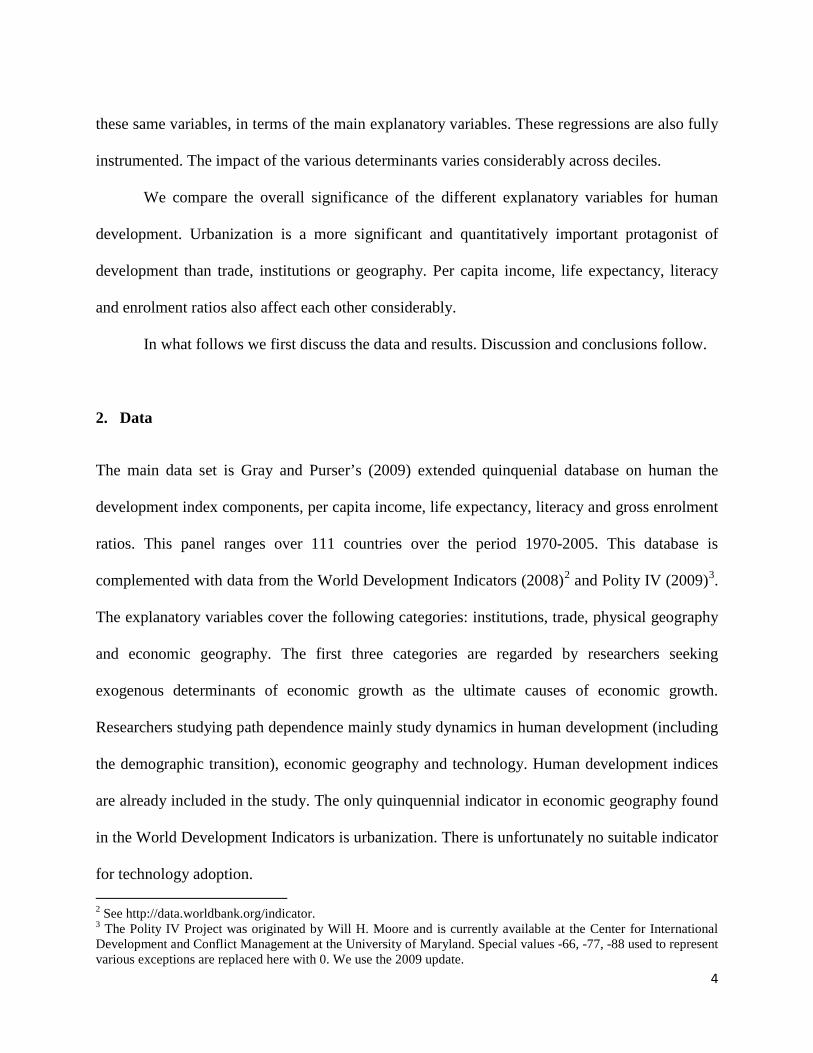
Now, the fact of the matter is that this area of study, centered mainly on conditional

convergence regressions, has produced a vast literature but nebulous results. A well-known

investigation found that “the cross-country statistical relationship between long-run average

growth rates and almost every particular macroeconomic indicator is fragile to small changes in

the conditioning information set” (Levine & Renelt, 1992). This research also found “qualified

support for the conditional-convergence hypothesis: a robust, negative correlation between the

initial level income and growth over the 1960-1989 period when the equation includes a measure

of the initial level of investment in human capital,” implying, as mentioned above, that human

capital is a slow moving variable reflecting the deeper inertias that define development and

3

underdevelopment. Another well-known investigation used two million regressions to find that

regional dummies, political variables such as rule of law or political rights, religion, market

distortions and performance, types of investment, fraction of primary products in total exports or

of GDP in mining, openness, type of economic organization, and colonial history were on the

whole significant determinants of economic growth (Sala-i-Martin, 1997).

What these studies show is that economic and human development are complex processes

with historical, political, economic, institutional and geographical determinants that do not

conform to some simple linear model.

To throw light on the evolution of human development over the period 1970-2005, I first

conduct a descriptive study of the indicators of human development and of some of the main

explanatory variables. The main conclusion is that economic development consists of a series of

nonlinear transitions, characterized by an initial period of divergence followed by a subsequent

period of convergence.

Next I conduct two sets of estimates on cross country differences that evaluate two

different aspects of growth. One is an estimate on the divergence/convergence of the human

development index (HDI) components. This estimate decomposes the (absolute) convergence

coefficient for each of these four indicators, to find what explanatory variables contribute to their

convergence or divergence. To take into account the complex interaction which exists between

the different economic variables, these regressions are fully instrumented. There are variables

contributing to both convergence and divergence. Variables contributing to divergence are more

critical to the growth process because they exhibit impact thresholds and increasing returns.

The other set of estimates concentrates on differences in HDI component levels across

countries. It consists of quantile regressions for the determinants of these levels across deciles of

4

these same variables, in terms of the main explanatory variables. These regressions are also fully

instrumented. The impact of the various determinants varies considerably across deciles.

We compare the overall significance of the different explanatory variables for human

development. Urbanization is a more significant and quantitatively important protagonist of

development than trade, institutions or geography. Per capita income, life expectancy, literacy

and enrolment ratios also affect each other considerably.

In what follows we first discuss the data and results. Discussion and conclusions follow.

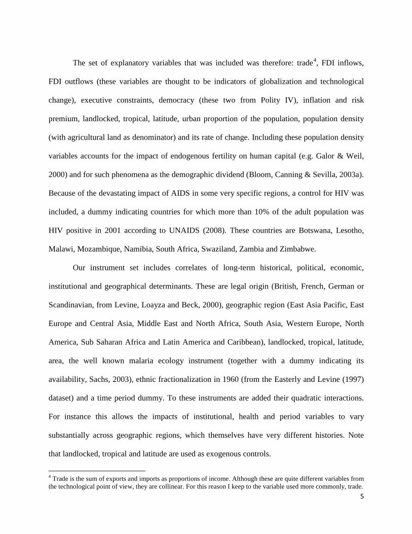
2. Data

The main data set is Gray and Purser’s (2009) extended quinquenial database on human the

development index components, per capita income, life expectancy, literacy and gross enrolment

ratios. This panel ranges over 111 countries over the period 1970-2005. This database is

complemented with data from the World Development Indicators (2008)2 and Polity IV (2009)3

2 See http://data.worldbank.org/indicator.

.

The explanatory variables cover the following categories: institutions, trade, physical geography

and economic geography. The first three categories are regarded by researchers seeking

exogenous determinants of economic growth as the ultimate causes of economic growth.

Researchers studying path dependence mainly study dynamics in human development (including

the demographic transition), economic geography and technology. Human development indices

are already included in the study. The only quinquennial indicator in economic geography found

in the World Development Indicators is urbanization. There is unfortunately no suitable indicator

for technology adoption.

3 The Polity IV Project was originated by Will H. Moore and is currently available at the Center for International Development and Conflict Management at the University of Maryland. Special values -66, -77, -88 used to represent various exceptions are replaced here with 0. We use the 2009 update.

5

The set of explanatory variables that was included was therefore: trade4

Our instrument set includes correlates of long-term historical, political, economic,

institutional and geographical determinants. These are legal origin (British, French, German or

Scandinavian, from Levine, Loayza and Beck, 2000), geographic region (East Asia Pacific, East

Europe and Central Asia, Middle East and North Africa, South Asia, Western Europe, North

America, Sub Saharan Africa and Latin America and Caribbean), landlocked, tropical, latitude,

area, the well known malaria ecology instrument (together with a dummy indicating its

availability, Sachs, 2003), ethnic fractionalization in 1960 (from the Easterly and Levine (1997)

dataset) and a time period dummy. To these instruments are added their quadratic interactions.

For instance this allows the impacts of institutional, health and period variables to vary

substantially across geographic regions, which themselves have very different histories. Note

that landlocked, tropical and latitude are used as exogenous controls.

, FDI inflows,

FDI outflows (these variables are thought to be indicators of globalization and technological

change), executive constraints, democracy (these two from Polity IV), inflation and risk

premium, landlocked, tropical, latitude, urban proportion of the population, population density

(with agricultural land as denominator) and its rate of change. Including these population density

variables accounts for the impact of endogenous fertility on human capital (e.g. Galor & Weil,

2000) and for such phenomena as the demographic dividend (Bloom, Canning & Sevilla, 2003a).

Because of the devastating impact of AIDS in some very specific regions, a control for HIV was

included, a dummy indicating countries for which more than 10% of the adult population was

HIV positive in 2001 according to UNAIDS (2008). These countries are Botswana, Lesotho,

Malawi, Mozambique, Namibia, South Africa, Swaziland, Zambia and Zimbabwe.

4 Trade is the sum of exports and imports as proportions of income. Although these are quite different variables from the technological point of view, they are collinear. For this reason I keep to the variable used more commonly, trade.

6

Descriptive statistics for all of the variables are presented in Table 1.

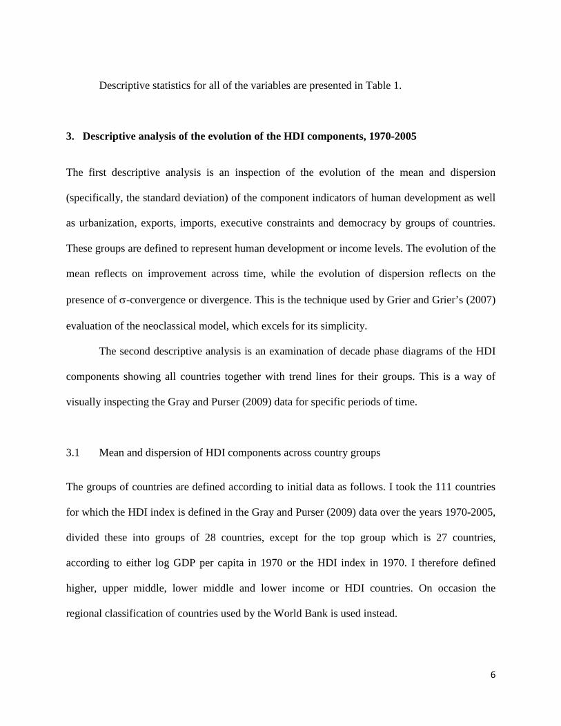
3. Descriptive analysis of the evolution of the HDI components, 1970-2005

The first descriptive analysis is an inspection of the evolution of the mean and dispersion

(specifically, the standard deviation) of the component indicators of human development as well

as urbanization, exports, imports, executive constraints and democracy by groups of countries.

These groups are defined to represent human development or income levels. The evolution of the

mean reflects on improvement across time, while the evolution of dispersion reflects on the

presence of σ-convergence or divergence. This is the technique used by Grier and Grier’s (2007)

evaluation of the neoclassical model, which excels for its simplicity.

The second descriptive analysis is an examination of decade phase diagrams of the HDI

components showing all countries together with trend lines for their groups. This is a way of

visually inspecting the Gray and Purser (2009) data for specific periods of time.

3.1 Mean and dispersion of HDI components across country groups

The groups of countries are defined according to initial data as follows. I took the 111 countries

for which the HDI index is defined in the Gray and Purser (2009) data over the years 1970-2005,

divided these into groups of 28 countries, except for the top group which is 27 countries,

according to either log GDP per capita in 1970 or the HDI index in 1970. I therefore defined

higher, upper middle, lower middle and lower income or HDI countries. On occasion the

regional classification of countries used by the World Bank is used instead.

7

As it happens, literacy is the variable that most closely follows the paradigm of absolute

convergence. This is because the proportion of the population that can be literate has a natural

upper bound (the whole population, actually 0.99 in our database), and because one of the factors

of production of this good–teachers–consists of literate people themselves, independently of their

level of income. The good itself–literacy–is not subject to much technological change, and fairly

high levels of literacy have been obtained by many less developed countries. Between 1970 and

2005 mean literacy for the 111 countries increased from 0.62 to 0.83 and the standard deviation

decreased almost linearly from 0.30 to 0.18. Even so, there is one difference with the usual

paradigm, and this is that the initial phase of literacy growth is divergent.

Figures 1.1 and 1.2 show the trajectories of mean and standard deviation for four groups

of countries, defined according to income or human development levels. Each trajectory consists

of eight points corresponding to the quinquennial series 1970-2005, that shift towards the right

unless otherwise indicated. It can be observed that once mean literacy reaches a level of

approximately 0.5, the dispersion of literacy across both income and human development groups

diminishes as group mean literacy increases. Also, the value mean literacy tends to converge to

is common across groups: the maximum possible value, when all of the population is literate.

These trajectories are most clearly distinct across human development groups, showing this

grouping defines the dynamic of the variable itself better than the income grouping.

So far, this describes absolute convergence. However, the initial segments of the

trajectories traversed by the lowest income or human development groups, when literacy is less

than approximately 0.5, follow divergent trajectories, since as literacy increases so does its

dispersion. This shows that literacy growth takes off in different countries at different times.

8

The two qualitatively different segments of the trajectories, first divergence and then

convergence, together constitute a transition, in this case from illiteracy to literacy.

Let us now turn to log per capita GDP. In this case both the mean and standard deviation

across the 111 countries increased, from 8.2 to 8.7, and from 1.27 to 1.41 respectively. However,

a closer look shows Figures 2.1 is consistent with a long-term transition in income for the three

highest groups, while the bottom group is trapped. The mean is not marked by improvement.

Figure 2.2 also shows the bottom group trapped, but this time the top groups form a convergence

club pattern, the top group apparently converging to a higher equilibrium, as the linear trend

lines show. These conclusions are consistent with other well-known research. Quah (1996) finds

evidence for a twin-peaked distribution. Bloom, Canning & Sevilla (2003b), find evidence for an

income poverty trap. Castellacci (2006, 2008) finds evidence for three technology convergence

clubs consistent with the theory in Howitt and Mayer-Foulkes (2005). Mayer-Foulkes (2006)

finds evidence for three convergence clubs with divergence as well as transitions between them.

Life expectancy shows a somewhat different evolution to per capita income or literacy.

Mean life expectancy across the 111 countries increased from 58 to 68 years, while the standard

deviation went from 10.1 to 11.1, partly because of the increasing life expectancy at the top end

of the spectrum. Figures 3.1 and 3.2 shows a transition in which countries are eventually tending

to similar life expectancy levels. If only the first five points of each trajectory are considered,

from 1970 to 1990, the diagrams a transition ending with a convergence almost as sharp as for

literacy. The transition is clearest by human development groups. However, around 1990

dispersion begins increasing in the three lower groups. Also, human development groups 1 and 2

have experienced a consistent increase in life expectancy since 1995, without an increase in

dispersion. This changing pattern from convergence to divergence is documented in a series of

9

works. Moser, Shkolnikov & Leon (2005) show that life expectancy divergence replaced

convergence in the late 1980’s because of adult mortality differences. These results are supported

by McMichael et al (2004). A trend from convergence to divergence in the late 20th century is

also noted by Taylor (2009). Ram (2006) shows that, instead of the sharp convergence before the

1980’s, after 1980 there is lack of convergence and an indication of “divergence,” that is

particularly marked during the 1990s. Also noted is substantial heterogeneity across the top and

the bottom quartiles within each period. Increases in world life span inequality are also noted by

Edwards (2010).

Gross enrolment ratios represent the proportion of the schooling age population enrolled

in primary, secondary, and tertiary education. Figures 4.1 and 4.2 show the evolution of these

rates across time and across country groups. Because schooling follows discrete stages,

enrolment ratios increase by waves across time. This is most clearly seen by income groups.

Apparently higher education levels are undertaken when income resources permit, and when this

occurs, a rise in dispersion follows. 19 out of 31 human development group 1 countries had

reached enrolment ratios above 0.9 by 2005. The mean gross enrolment rate across the 111

countries is somewhat meaningless. It increased from 0.49 to 0.72, while the standard deviation

fluctuated from 0.20 down 0.18 and then back to 0.19.

3.2 Decade phase diagrams for the evolution of HDI components across country groups

A closer examination of the evolution of HDI components across country groups is provided by

decade phase diagrams that show levels of some indicator on the x axis and its change across a

decade on the y axis.

10

We begin again with literacy, because it illustrates a transition that begins with a period

of divergence and ends with absolute convergence. Figure 5.1 shows decade phase diagrams

across regional country groups beginning in 1970, Figure 5.2 beginning in 1995. The 1970

diagram shows Sub Saharan Africa and South Asia in the initial divergent stage of the literacy

transition, with the rest of the regions already converging towards a literacy rate of 1. By 1995

all of the regions had reached the convergent phase of the transition.

Log per capita income follows quite a complex process. Figure 6.1 illustrates income

growth from 1980 to 1990 across income groups. Here the higher income group is divided into

OECD and non-OECD countries. All of the groups except for the OECD countries are following

a pattern of club convergence, while higher OECD countries appear to be experiencing a new

phase of growth. This coincides with the initial phase of the wave of globalization that begun in

the 1990’s. Ten years later, in 1990 (Figure 6.2), all groups of countries are growing towards

higher equilibriums, especially the non-OECD higher income group, which exhibits some

divergence, but also the lowest income group. The full pattern is one of a sequence of transitions

that begin with a divergent phase and then follow a convergent pattern that might exhibit club

convergence or delayed entrance into later transitions.

Figure 7.1, a life expectancy phase diagram for the 1970 to 1980 decade across

geographical regions, shows a typical transition pattern. However, the most advanced regions are

converging towards higher levels of life expectancy. By 1995, though (Figure 7.2) Sub Saharan

Africa had experienced a life expectancy disaster (due to HIV and war). It was now converging

towards a life expectancy level of only 55 years. Meanwhile South Asia was experiencing a new

spurt of transition in life expectancy.

11

A similar pattern occurred for the gross enrolment ratio. Figure 8.1 shows for the decade

beginning in 1970 a convergent pattern for gross enrolment to levels of 0.8, except for

divergence in Eastern Europe and Central Asia, and convergence to very low levels in South

Asia. By the decade beginning 1995 (Figure 8.2) Western Europe and North America, East

Europe and Central Asia, and Latin America and Caribbean have completed transition phases

and are now converging to higher equilibriums. Meanwhile East Asia Pacific, Middle East and

North Africa, and South Asia are entering transitional phases with lower initial levels.

Figure 8 shows Sub Saharan Africa’s life expectancy evolution over the full period 1970-

1995 in more detail. The decades beginning 1970, 1975 and 1980 show divergent transitional

phases. 1985, 1990 and 1995 instead show convergent phases, towards lower levels of

dispersion, but also to lower steady state levels falling to 53 years in 1990 and then rising to 55

in 1995. Some countries display 15 years loses in life expectancy in the decade beginning 1995.

3.3 Mean and dispersion of the main explanatory variables

We now conduct a descriptive analysis of our main explanatory variables. One of the

motivations is to see whether these variables offer particularly striking instances of divergence or

convergence. We consider the evolution of the mean and dispersion of urbanization, exports,

imports, executive constraints and democracy in the same way as we did for the human

development indicators.

Figure 9.1 shows a surprisingly intimate relation between urbanization and income levels.

The trajectories of urbanization across lower and middle income groups form an almost perfectly

integrated common trajectory of increasing means and standard deviations. Meanwhile, the

higher income group also increased its urbanization rate, but at a lower level of dispersion

12

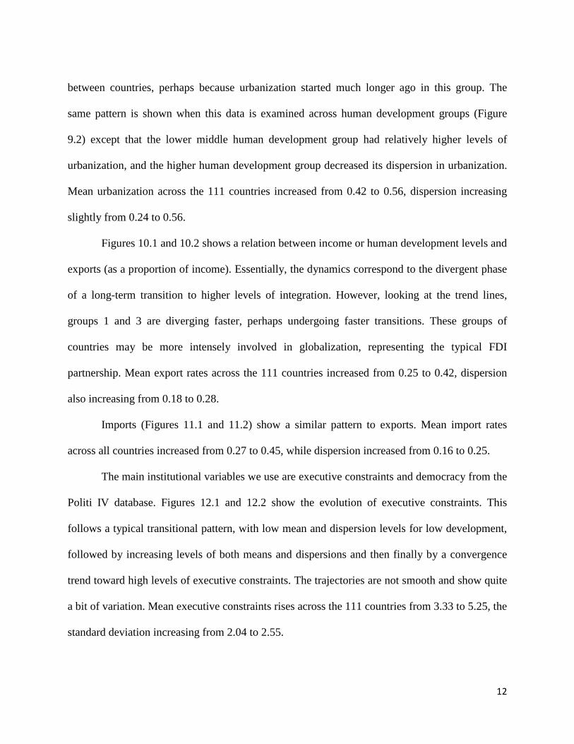
between countries, perhaps because urbanization started much longer ago in this group. The

same pattern is shown when this data is examined across human development groups (Figure

9.2) except that the lower middle human development group had relatively higher levels of

urbanization, and the higher human development group decreased its dispersion in urbanization.

Mean urbanization across the 111 countries increased from 0.42 to 0.56, dispersion increasing

slightly from 0.24 to 0.56.

Figures 10.1 and 10.2 shows a relation between income or human development levels and

exports (as a proportion of income). Essentially, the dynamics correspond to the divergent phase

of a long-term transition to higher levels of integration. However, looking at the trend lines,

groups 1 and 3 are diverging faster, perhaps undergoing faster transitions. These groups of

countries may be more intensely involved in globalization, representing the typical FDI

partnership. Mean export rates across the 111 countries increased from 0.25 to 0.42, dispersion

also increasing from 0.18 to 0.28.

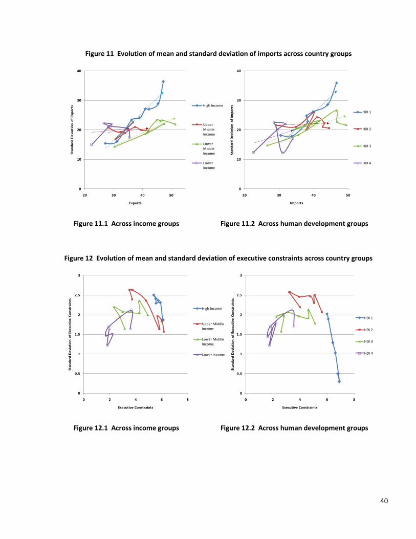
Imports (Figures 11.1 and 11.2) show a similar pattern to exports. Mean import rates

across all countries increased from 0.27 to 0.45, while dispersion increased from 0.16 to 0.25.

The main institutional variables we use are executive constraints and democracy from the

Politi IV database. Figures 12.1 and 12.2 show the evolution of executive constraints. This

follows a typical transitional pattern, with low mean and dispersion levels for low development,

followed by increasing levels of both means and dispersions and then finally by a convergence

trend toward high levels of executive constraints. The trajectories are not smooth and show quite

a bit of variation. Mean executive constraints rises across the 111 countries from 3.33 to 5.25, the

standard deviation increasing from 2.04 to 2.55.

13

A similar pattern of transition is found for democracy in Figures 13.1 and 13.2. From

1975 to 2005 the mean across the 111 countries rises from 1.89 to 3.58 and the standard

deviation from 3.97 to 4.17.

In contrast to Acemoglu, Johnson and Robinson (2002, 2005), who propose that the

critical feature of success in development had been the quality of the institutional framework

inherited since colonial times, which they consider to be for all intents and purposes fixed across

time, both executive constraints and democracy are clearly following a transition. Approximately

three fourths of all countries are still in the divergent phase, with only the top fourth beginning to

converge. It is illustrative to note that the case of literacy is the reverse: the bottom fourth is still

in the divergent phase of the transition, while the top three fourths are in the convergent phase.

Summarizing, the main feature revealed by the descriptive analysis is that human

development, as well as its determinants, follow a series of superposed transitions that first take

off with increasing divergence and then converge to a higher equilibrium. This very fundamental

feature of development is almost completely missing in most theoretical models on economic

growth. It could be said that vicious cycles keep transitions from beginning. Once they begin,

they are characterized by virtuous cycles that reach a higher equilibrium.

4. Decomposition of the convergence coefficient

The descriptive exploration has shown that the evolution of the HDI components is characterized

by a complex pattern of convergence and divergence. It consists of a series of superposed

transitions that first take off with increasing divergence and then converge, smoothly in some

exceptional cases and exhibiting more complexity and turbulence in others. Also, a series of

14

events such as HIV, war, globalization, or regime changes in Eastern Europe and Central Asia,

India, China, and so on, strongly affect the course of this evolution.

In what follows we carry out an econometric analysis to investigate whether some causal

variables are particularly related to convergence or divergence.

4.1 Estimation

One way of investigating convergence and divergence is to introduce interaction terms in the

convergence term in regressions on the rate of growth, of income for example. Here we extend

this method, used for example in Aghion, Howitt and Mayer-Foulkes (2005), as follows.

I consider that utility is approximately linear in life expectancy, literacy and enrolment

ratios, only per capita income needing to be considered as a logarithm. Thus in his section when

we talk about HDI components log per capita income stands in place of per capita income.

The convergence decomposition estimates are the following. For each HDI component

consider the convergence decomposition regression

where index t over periods 1970, 1975, … , 2000 and index i ranges over 85 countries

constituting a balanced panel (the explanatory variables do not cover the 111 countries). Here

are the explanatory variables to be instrumented, including the HDI components. The

convergence coefficient is decomposed as . It is necessary to include the independent

terms so as not to introduce omitted variable bias. We include a very limited number of

controls that are not interacted with the convergence term, specifically the AIDS dummy, and

the physical geography variables landlocked, tropical and latitude. These are therefore

15

considered to have level but not growth effects5. are time period dummies6

These regressions are evaluated simultaneously using 3SLS, and individually using

clustered errors. Explanatory variables are instrumented using the instruments listed in the

data section. Exogenous variables of course intervene in the first stage regressions

. ujt

are the stochastic terms. Finally are the coefficients.

7

The only instruments providing variation across time are the period dummies. In a sense

the panel estimates therefore provide an enriched cross section. For this reason it is to be

expected that the error structure is clustered, showing correlation across time for each country.

Clustered errors turn out to be the best estimates because the instrument set satisfies the

Hausman and Sargan tests in this case. It also turns out that the 3SLS estimate results are not

very different when the regressions for the HDI components are evaluated individually or

simultaneously.

. Inclusion

of the quadratic interactions of the instruments is justified not only on the grounds mentioned

above that the impacts of the various instruments can vary across geographic regions (these are

also historical correlates), but also because the presence of the quadratic interaction terms of the

independent variables calls for them. At the same time these interactions serve to augment the

instrument set’s dimension, allowing the simultaneous instrumentation of variables , each of

which can be considered endogenous.

4.2 Results

5 When the physical geography variables were interacted the 3SLS estimation did not converge. 6 The quinquennial fixed effects can be thought to include the technological leading edge in the HDI component being evaluated (see Aghion, Howitt and Mayer-Foulkes, 2005). 7 The AIDS dummy defines a contiguous region that approximately coincides with the region south of the 18th southern parallel in Africa. I consider that the social and geographic conditions that established this region as a contagion basin for AIDS already existed in 1970, and therefore consider the AIDS dummy to be exogenous.

16

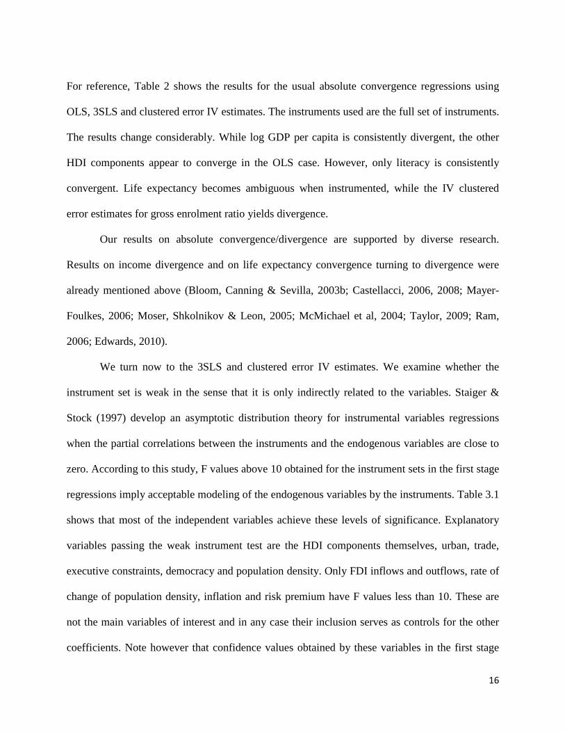
For reference, Table 2 shows the results for the usual absolute convergence regressions using

OLS, 3SLS and clustered error IV estimates. The instruments used are the full set of instruments.

The results change considerably. While log GDP per capita is consistently divergent, the other

HDI components appear to converge in the OLS case. However, only literacy is consistently

convergent. Life expectancy becomes ambiguous when instrumented, while the IV clustered

error estimates for gross enrolment ratio yields divergence.

Our results on absolute convergence/divergence are supported by diverse research.

Results on income divergence and on life expectancy convergence turning to divergence were

already mentioned above (Bloom, Canning & Sevilla, 2003b; Castellacci, 2006, 2008; Mayer-

Foulkes, 2006; Moser, Shkolnikov & Leon, 2005; McMichael et al, 2004; Taylor, 2009; Ram,

2006; Edwards, 2010).

We turn now to the 3SLS and clustered error IV estimates. We examine whether the

instrument set is weak in the sense that it is only indirectly related to the variables. Staiger &

Stock (1997) develop an asymptotic distribution theory for instrumental variables regressions

when the partial correlations between the instruments and the endogenous variables are close to

zero. According to this study, F values above 10 obtained for the instrument sets in the first stage

regressions imply acceptable modeling of the endogenous variables by the instruments. Table 3.1

shows that most of the independent variables achieve these levels of significance. Explanatory

variables passing the weak instrument test are the HDI components themselves, urban, trade,

executive constraints, democracy and population density. Only FDI inflows and outflows, rate of

change of population density, inflation and risk premium have F values less than 10. These are

not the main variables of interest and in any case their inclusion serves as controls for the other

coefficients. Note however that confidence values obtained by these variables in the first stage

17

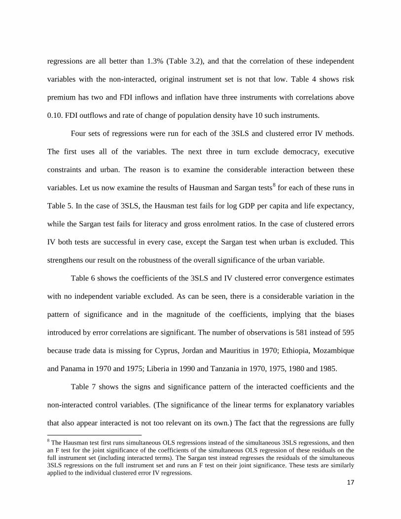
regressions are all better than 1.3% (Table 3.2), and that the correlation of these independent

variables with the non-interacted, original instrument set is not that low. Table 4 shows risk

premium has two and FDI inflows and inflation have three instruments with correlations above

0.10. FDI outflows and rate of change of population density have 10 such instruments.

Four sets of regressions were run for each of the 3SLS and clustered error IV methods.

The first uses all of the variables. The next three in turn exclude democracy, executive

constraints and urban. The reason is to examine the considerable interaction between these

variables. Let us now examine the results of Hausman and Sargan tests8

Table 6 shows the coefficients of the 3SLS and IV clustered error convergence estimates

with no independent variable excluded. As can be seen, there is a considerable variation in the

pattern of significance and in the magnitude of the coefficients, implying that the biases

introduced by error correlations are significant. The number of observations is 581 instead of 595

because trade data is missing for Cyprus, Jordan and Mauritius in 1970; Ethiopia, Mozambique

and Panama in 1970 and 1975; Liberia in 1990 and Tanzania in 1970, 1975, 1980 and 1985.

for each of these runs in

Table 5. In the case of 3SLS, the Hausman test fails for log GDP per capita and life expectancy,

while the Sargan test fails for literacy and gross enrolment ratios. In the case of clustered errors

IV both tests are successful in every case, except the Sargan test when urban is excluded. This

strengthens our result on the robustness of the overall significance of the urban variable.

Table 7 shows the signs and significance pattern of the interacted coefficients and the

non-interacted control variables. (The significance of the linear terms for explanatory variables

that also appear interacted is not too relevant on its own.) The fact that the regressions are fully 8 The Hausman test first runs simultaneous OLS regressions instead of the simultaneous 3SLS regressions, and then an F test for the joint significance of the coefficients of the simultaneous OLS regression of these residuals on the full instrument set (including interacted terms). The Sargan test instead regresses the residuals of the simultaneous 3SLS regressions on the full instrument set and runs an F test on their joint significance. These tests are similarly applied to the individual clustered error IV regressions.

18

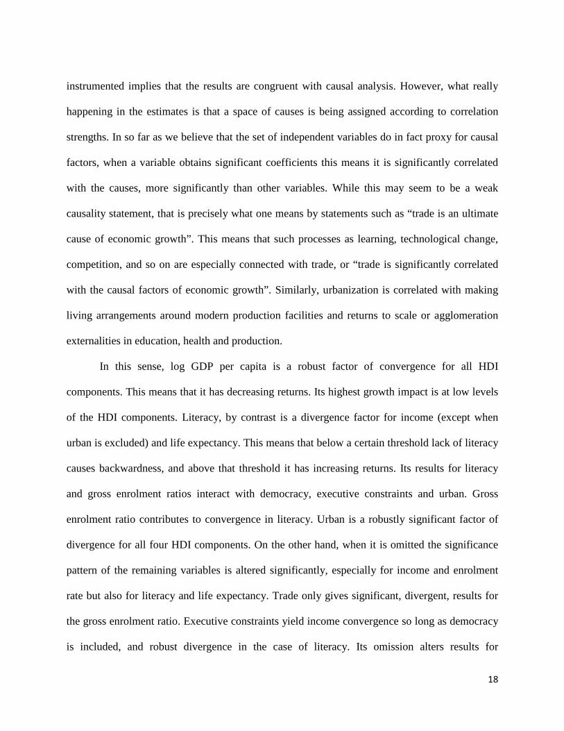
instrumented implies that the results are congruent with causal analysis. However, what really

happening in the estimates is that a space of causes is being assigned according to correlation

strengths. In so far as we believe that the set of independent variables do in fact proxy for causal

factors, when a variable obtains significant coefficients this means it is significantly correlated

with the causes, more significantly than other variables. While this may seem to be a weak

causality statement, that is precisely what one means by statements such as “trade is an ultimate

cause of economic growth”. This means that such processes as learning, technological change,

competition, and so on are especially connected with trade, or “trade is significantly correlated

with the causal factors of economic growth”. Similarly, urbanization is correlated with making

living arrangements around modern production facilities and returns to scale or agglomeration

externalities in education, health and production.

In this sense, log GDP per capita is a robust factor of convergence for all HDI

components. This means that it has decreasing returns. Its highest growth impact is at low levels

of the HDI components. Literacy, by contrast is a divergence factor for income (except when

urban is excluded) and life expectancy. This means that below a certain threshold lack of literacy

causes backwardness, and above that threshold it has increasing returns. Its results for literacy

and gross enrolment ratios interact with democracy, executive constraints and urban. Gross

enrolment ratio contributes to convergence in literacy. Urban is a robustly significant factor of

divergence for all four HDI components. On the other hand, when it is omitted the significance

pattern of the remaining variables is altered significantly, especially for income and enrolment

rate but also for literacy and life expectancy. Trade only gives significant, divergent, results for

the gross enrolment ratio. Executive constraints yield income convergence so long as democracy

is included, and robust divergence in the case of literacy. Its omission alters results for

19

democracy and other variables. Democracy yields divergence in incomes so long as executive

constraints are included, and divergence in enrolment ratios so long as urban is included. Its

omission alters results for executive constraints and other variables. FDI inflows are a factor of

convergence in literacy and enrolment ratios. FDI outflows are a factor of divergence in life

expectancy and gross enrolment ratio and of convergence in literacy. Population density is a

factor of divergence in life expectancy and convergence in enrolment rates. Population density

growth is only significant when urban is excluded. Low risk premiums, (correcting for its

negative quality by changing the signs) contribute to convergence in literacy and divergence in

enrolment rates. Similarly, low inflation contributes to divergence in life expectancy, literacy and

enrolment rates.

Turning to non-interacted controls, AIDS decreases life expectancy and increases GDP

per capita (through mortality). Landlocked reduces income and life expectancy somewhat

significantly, when no variables are omitted. Tropical reduces GDP and literacy. Latitude

increases income, life expectancy and literacy but reduces the enrolment ratio.

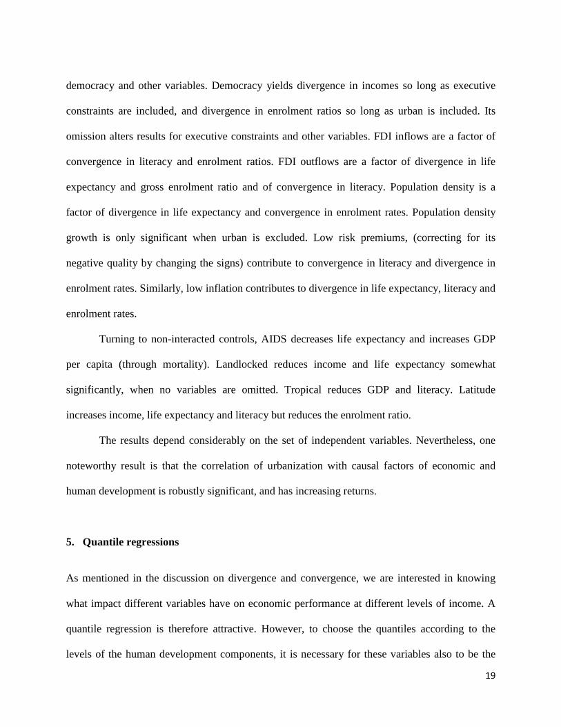
The results depend considerably on the set of independent variables. Nevertheless, one

noteworthy result is that the correlation of urbanization with causal factors of economic and

human development is robustly significant, and has increasing returns.

5. Quantile regressions

As mentioned in the discussion on divergence and convergence, we are interested in knowing

what impact different variables have on economic performance at different levels of income. A

quantile regression is therefore attractive. However, to choose the quantiles according to the

levels of the human development components, it is necessary for these variables also to be the

20

dependent variables. This is possible if we conduct a levels rather than growth estimate. Also, we

need to instrument the independent variables so that we can estimate each of the components in

terms of the others as well as all of the independent variables. The quantile levels we consider

are 0.1 to 0.9. We include the time dummies only as instruments and not as controls because the

quantile regressions do not converge when they are included, there probably are already too

many constants in the estimates, one for each quantile level. Explanatory variables tX are

substituted with their predicted values from the first stage of instrumental equations before

running the quantile estimates9

.

5.1 Results

The results are shown in Tables 8.1 to 8.4. There are many significant results and they vary

considerably at different quantiles. We examine the results graphically in Figures 14.1 to 14.4.

To do so we plot the coefficients with a higher t value than 1.96 (corresponding to a significance

of approximately 5%) multiplied by one standard deviation. This measures the impact of a

change of one standard deviation on the target HDI component.

This exercise does not include the physical geography variables, which are not subject to

policy. However, these variables obtained significant results. Latitude was positive when

significant for income and life expectancy, and negative for literacy. It was not significant for

enrolment ratios. Latitude may be embodying omitted variables in technology, colonial history,

and so on. Landlocked was positive when significant for income, mostly negative for life

9 All of the estimates were carried out with Stata. Each quantile regression was carried out separately. Fifty weighted least-squares iterations were estimated before the linear programming iterations were started.

21

expectancy, positive for literacy and negative for enrolment ratios, in somewhat surprising

results. Tropical was negative when significant for income, life expectancy, and enrolment ratios,

and positive for literacy. Next come literacy and executive constraints, exhibiting decreasing

impact with income level. Democracy, FDI inflows and inflation appear with negative signs.

Figure 14.1 shows the quantile results for income. The variables with most impact are life

expectancy and urbanization. Interestingly, life expectancy is not only affecting lower but also

higher income levels. Work on the impact of health on income has previously emphasized the

impact of health at lower income levels (for a summary see Bloom & Canning, 2008). The

impacts at higher income levels may be related to transitions in the last 20 years. In contrast,

urbanization affects middle income levels more strongly, making it a development tool for a

wide range of underdeveloped countries.

Figure 14.2 shows the results for life expectancy. Literacy, democracy, income,

urbanization, trade, population and FDI inflows have a positive impact, while executive

constraints, population growth, FDI outflows, and risk premium have a negative impact. The

indicators exhibit a high degree of significance and all of the signs are the expected signs except

perhaps for executive constraints. While some indicators show decreasing returns, others peak at

medium high levels of life expectancy, such as urbanization, yet others at the top levels, such as

enrolment ratios.

Figure 14.3 shows the results for literacy. Enrolment ratio, life expectancy, FDI outflows,

and executive constraints are the variables with the most consistent positive impact. Democracy,

urbanization, trade (for lower levels of literacy) and population growth are the variables with the

most consistent negative impact.

22

Figure 14.4 shows the results for enrolment ratios. Literacy (for all levels of enrolment),

urbanization and GDP (at lower levels of enrolment), democracy, population and trade (at

intermediate levels), life expectancy, FDI outflows and population growth (for higher levels), are

significant.

6. Discussion

6.1 The most significant results

What have we learned from our analysis? We can start by comparing the results of the two sets

of estimates. Note that the convergence coefficients represent the marginal growth and the

quantile estimates the marginal level that each independent variable can provide for each HDI

component. Table 9 represents the signs and significance of the main coefficients in both sets of

estimates. In the case of the convergence estimates the preferred run is the clustered error IV,

with no variable omitted. Our significance measure is the sum of the number of significance stars

obtained by each variable for each sign. This measure is closely correlated with just counting the

number of times a variable is significant in each sign. In the case of quantile regression

coefficients, we count the number of quantiles each variable was significant for, for each sign.

We comment on the explanatory variables in the order of their total significance scores.

Urbanization is the most significant. While it has some negative level effects, it has consistently

increasing returns to growth (of HDI components). Literacy is always positive for levels and also

has consistently increasing returns to growth. Income is equally significant, always positive in

levels but always has decreasing returns to growth. Next is democracy, with positive and

negative impact levels, but increasing returns to growth. Executive constraints follows, equally

23

ambiguous in levels, but with some increasing and some decreasing returns to growth. Then

comes life expectancy, always positive in levels, but with decreasing returns, like income. Trade

is as significant as life expectancy, ambiguous in levels but with increasing returns. Low

inflation has ambiguous level effects but increasing returns. FDI inflows also has ambiguous

level effects but instead decreasing returns. Then come FDI outflows, population density and its

growth, with ambiguous level and growth effects, although FDI outflows stands out for

increasing returns.

In order of significance, urbanization, low inflation, FDI outflows, literacy and

democracy stand out for their increasing returns to HDI component growth. This is an aspect of

growth that the prevalent emphasis on convergence has missed studying. Similarly literacy,

urbanization, life expectancy, income and trade, in that order, stand out for their positive

contributions to levels of the HDI components.

There are several salient results. First is the consistent significance of urban proportion of

the population. It affects income, literacy and gross enrolment ratio. All of its signs are positive

and the magnitudes significant except for the literacy quantile estimate. This may be a reflection

of migrant poverty. Given the consistent impact of cities, it is surprising that they do not impact

life expectancy significantly. Perhaps they have significant positive and negative effects.

Once one thinks about it, it is quite reasonable that cities play an important role in

development, given that modern technologies and life are mainly city based. The reason the

result is a surprise is that cities do not figure very much in development analysis or policy.

Another surprise is that trade does not significantly impact income. It does significantly

affect life expectancy levels. This may work through increasing the availability of myriad cheap

technologies to improve health, as well as cheap food. It may also complement knowledge

24

channels significantly associated here with life expectancy, such as literacy and gross enrolment

ratio. Trade is also significantly associated with the gross enrolment ratio and its growth.

Low inflation is positively associated with income levels and yields increasing returns in

the other HDI components.

As far as the set of exogenous variables are concerned, which include the “ultimate

causes of growth,” economic geography yields far more significant impacts than trade, FDI or

institutions. This kind of geographic variable is not the kind of physical geography, exogenous

variable that is included in ultimate causes. Instead, it refers to an important economic feature

that is not well coordinated by the market system.

While globalization has had large impacts, see for example Figure 14 showing how

income divergence (or dispersion) peaks in 1990, its main features, trade and FDI, have not had

the impact on the HDI components that might have been expected, according to the significance

patterns found here.

Another salient result is the ambiguity of the signs obtained by several important

explanatory variables across HDI components. This raises important questions. Why do

executive constraints, democracy, trade and FDI inflows and outflows and low inflation have

such mixed impacts? Are there issues of distribution that muddy the impacts of these

institutional, openness and macro management variables? The answer to this question might

yield very productive insights.

6.2 Towards objectivity

The modern theory of economic growth began with the neoclassical growth model, in some

sense a paradigm for the belief that markets are sufficient, or at least almost sufficient to direct

25

economic growth. The model assumes that competitive markets will allocate resources in such a

way as to produce optimal economic growth and economic convergence. Because much of

international economic life does in fact occur through markets, in evaluating cross-country

growth the model serves as a benchmark to see whether in fact the model explains growth, or if

not, what is going wrong.

For example, Grier and Grier (2007) note that to be consistent with the absolute

divergence in output levels – which they corroborate is occurring – it would be necessary to

observe divergence in some of the determinants of income, such as physical and human capital,

which they do not observe. However, they do observe divergence in technological levels. So this

is the first point – markets might not distribute technology optimally.

The neoclassical growth model can fail in two ways. If markets are a sufficient in

principle, then deficiencies might originate in the context that defines them – institutions,

(physical) geography and trade, this last being a basic policy choice. A considerable literature on

economic growth focuses on these types of causes as the fundamental causes of long-term

growth. Recently institutions seem to be the favorite of these causes (Rodrik and Subramanian,

2003; Rodrik, Subramanian and Trebbi, 2004).

Alternatively, markets are insufficient for regulating and coordinating substantial classes

of economic problems. For example, human capital investment is characterized by market

failures. Technology is based on market power. Urbanization is based on externalities. In

addition, public goods may be important. When such issues are strong enough, deficient market

equilibriums may arise, corresponding to persistent poverty. The lower equilibriums constitute,

by definition, traps that markets cannot dissolve.

26

Convergence and divergence are linked with these two possibilities. When markets drive

growth, convergence forces drive towards a new equilibrium. When markets are insufficient,

bottlenecks arise that slow growth and generate divergence between countries. When and if the

bottlenecks are overcome a transition emerges to an at least somewhat higher equilibrium.

Our descriptive study shows that development consists of a series of such superposed

transitions that first take off with increasing divergence and then converge to a higher

equilibrium. The paradigm of smooth growth is inconsistent with the facts.

The point is that the paradigm is deceptive. The reason is that conceptualizing growth as

a smooth process makes it appear that it is susceptible to uniform policies. When a transition is

ripe, it has increasing returns. When it is not, it may be impossible.

Miracle growth, which ought to be the objective of development policy, is a transition

from a low to a high steady state (see Wan’s 2004 case histories of East Asia) involving

transitions in production and in all aspects of economic life. It is not a simple, smooth process.

Markets will often bump into transitions on their own and carry them forward. However,

some transitions need public inputs and institutions. Aid programs in particular must recognize

which the relevant transitions are.

It is worth noting here that, at least conceptually, institutions fall into two kinds, those

that simply establish the market system, and those that play an additional economic, political or

social role. Providing public goods is not the least such role! Objectively, what types of

institutions are needed when?

It is of course possible that the market structure itself is impeded, creating a bottleneck,

but not all bottlenecks are solvable through markets. On the contrary, these barriers have

traditionally been the direct concern of public policy. The point is to let markets do what they do

27

well and complement what they do not. Western society has done this throughout its capitalist

history (with all the struggles this involves).

The discussion of convergence has tended to link with a radical defense of the

neoclassical growth model. However, what is needed is objectivity. When do markets carry

forward the growth process, and when do they not? What are the best ways to trigger the

transitions that are essential to development process? It is clear that well functioning markets are

a part of this, but claiming they are the whole throws the baby out with the bathwater.

Our convergence decomposition is a step towards objectivity. It shows that some

variables contribute to convergence and others to divergence. In turn, the quantile estimates

show that different variables are important at different levels of development. Moreover, several

of the crucial variables are not particularly well driven by the market, such as urbanization, life

expectancy, literacy and democracy.

6.3 Urbanization as an intermediate objective for development

Urbanization can be a particularly interesting intermediate objective for development for several

reasons. First, it is necessary. It is part of the development path. Perhaps given modern

technologies this includes making urban quality and externalities available to rural life. It

certainly means bringing quality to urban life. Many things go into organizing cities well, such as

transportation, provision of health and education, assigning areas for living and for industry and

services, and so on. It requires political and social organization. Also, each city in each context

will call for particular improvement objectives. These are all elements of a program of

development. On the other hand they are concrete. A way must also be found for markets to

determine some of the choices within some framework. Traditionally in underdeveloped

28

countries what has happened is that urbanization has proceeded in a disorganized way that turns

out to be very costly, governments following behind the facts.

In so far as urbanization has been important, it is not mainly making markets work better

that has achieved growth. Instead, it has been achieving the kind of social coordination that is

successful at creating cities that has obtained additional growth, together with the coordination

that markets can provide. The importance of this coordination and its institutional aspects is

illustrated by the interaction we have shown exists between the variables urban, democracy and

executive constraints.

7. Conclusions

Our descriptive analysis and estimates show that economic growth and development follow a

complex pattern of divergence and convergence. This can be thought to consist of a series of

superposed transitions that first take off with increasing divergence (and increasing returns) and

then converge.

Each human development component follows its own set of transitions. These are also

interlinked, in different ways at different stages. The estimates confirm the complex relations in

divergence and convergence that exist in these indicators.

Our estimates include indicators of the “ultimate causes of economic growth,”

institutions, trade and physical geography. They also include an indicator in economic

geography, proportion of the urban population. The descriptive analysis has found evidence of

divergence in the evolution of urbanization, exports and imports (Figures 9, 10, 11). It also found

strong evidence that executive constraints and democracy follow an endogenous –if more

complex– transition analogous to other variables such as literacy (Figures 1, 12, 13).

29

The results show that economic geography is more significant to economic and human

development than either trade or the market-institutional indicators (executive constraints, risk

premium and inflation), and that, as any variable contributing to divergence, has increasing

returns to growth.

There is also evidence that institutional and openness variables such as democracy and

executive constraints, trade and FDI inflows, have both significantly positive and significantly

negative impacts. Perhaps this is due to their distributive effects. It may be that policies for

institutional improvement and openness could be more effective if their interactions with

distribution were addressed.

Meanwhile, improving markets will have smaller returns than complementing them with

adequate institutions capable of coordinating urbanization and investing in human capital and

technology. Urbanization itself can provide a concrete agenda for development addressing

critical local issues involving all aspects of economic, political and social life as well as human

development.

The neoclassical growth paradigm is wrong in another way as well. Economic

development is not a smooth process. Growth policies depend for their success in identifying a

set of transitions that a country is ripe for.

30

8. References

Acemoglu, Daron, Simon Johnson, and James A. Robinson (2005). Institutions as a Fundamental Cause of Long-Run Growth. In: Aghion, Philippe; Durlauf, Stefen (eds.). Handbook of Economic Growth. Amsterdam: North Holland.

Acemoglu, Daron, Simon Johnson, and James A. Robinson. (2002) “Reversal of Fortune: Geography and Institutions in the Making of the Modern World Income Distribution,” Quarterly Journal of Economics 117(4):1231-1294

Aghion, Howitt and Mayer-Foulkes (2005). “The Effect of Financial Development on Convergence: Theory and Evidence”, Quarterly Journal of Economics, 120(1), Feb.

Barro, R. (1991) “Economic Growth in a Cross Section of Countries. “ Quarterly Journal of Economics 196 (2/May): 407–443.

Bloom, David E.; Canning, David & Sevilla, Jaypee (2003a). “The Demographic Dividend: A New Perspective on the Economic Consequences of Population Change, Rand, MR-1274.

Bloom, David E; Canning, David & Sevilla, Jaypee (2003b). “Geography and Poverty Traps,” Journal of Economic Growth, Springer, vol. 8(4), pages 355-78, December.

Bloom, David E. & Canning, David (2008). “Population Health and Economic Growth.” The World Bank On behalf of the Commission on Growth and Development.

Castellacci, Fulvio (2008). “Technology clubs, technology gaps and growth trajectories,” Structural Change and Economic Dynamics, Elsevier, vol. 19(4), pages 301-314, December.

Castellaci, Fulvio (2006). “Convergence and Divergence among Technology Clubs,” DRUID Working Papers 06-21, DRUID, Copenhagen Business School, Department of Industrial Economics and Strategy/Aalborg University, Department of Business Studies.

Easterly, William and Levine, Ross (1997). “Africa’s Growth Tragedy: Policies and Ethnic Divisions,” Quarterly Journal of Economics 112, 1203-50, Nov.

Edwards, Ryan D. (2010). “Trends in World Inequality in Life Span Since 1970,” NBER Working Papers 16088, National Bureau of Economic Research, Inc.

Galor, Oded & Weil, David N. (2000). “Population, Technology, and Growth: From Malthusian Stagnation to the Demographic Transition and Beyond,” American Economic Review, Vol. 90, No. 4. (Sep), pp. 806-828.

Gray G. and M. Purser (2009). “Descriptive statistics and figures: Is it all really about income?”. HDRO, UNDP.

Grier K. and R. Grier (2007). “Only income diverges: A neoclassical anomaly”, Journal of Development Economics 84 (2007) 25–45.

Harris J. and M. Todaro (1970). Migration, Unemployment & Development: A Two-Sector Howitt, P. and Mayer-Foulkes, D. (2005). “R&D, Implementation and Stagnation: A

Schumpeterian Theory of Convergence Clubs”, Journal of Money, Credit and Banking, 37(1) February.

Levine, Ross, Norman Loayza, and Thorsten Beck (2000). “Financial Intermediation and Growth: Causality and Causes.” Journal of Monetary Economics 46, 31-77, August.

Mayer-Foulkes, D. (2006). “Global Divergence”, in Severov, Gleb, International Finance and Monetary Policy, Nova Science Publishers.

McMichael A.J., McKee M., Shkolnikov V. & Valkonen T. (2004). “Mortality trends and setbacks: global convergence or divergence?” Lancet. Apr 3;363(9415):1155-9.

31

Moser K., Shkolnikov V., Leon D.A. (2005). “World mortality 1950-2000: divergence replaces convergence from the late 1980s,” Bull World Health Organ. Mar;83(3):202-9.

Pritchett, Lant (1997). “Divergence, Big Time.” Journal of Economic Perspectives, 11(3), Summer 1997, pp. 3-17.

Quah, Danny T. (1996). “Twin Peaks: Growth and Convergence in Models of Distribution Dynamics,” Economic Journal, Royal Economic Society, vol. 106(437), pages 1045-55, July.

Ram, Rati (2006). “State of the “life span revolution” between 1980 and 2000,” Journal of Development Economics, Elsevier, vol. 80(2), pages 518-526, August.

Rodrik, Dani, Arvind Subramanian (2003) “The Primacy of Institutions (and what this does and does not mean),” Finance & Development 40(2): 1-4.

Rodrik, Dani, Arvind Subramanian and Francesco Trebbi. (2004) “Institutions Rule: The Primacy of Institutions over Geography and Integration in Economic Development” Journal of Economic Growth, vol. 9, no.2, June 2004

Sachs, J. D. (2003), “Institutions don’t rule: Direct effects of geography on per capita income”. NBER Working Paper 9490.

Sala-i-Martin, Xavier, 1997. “I Just Ran Two Million Regressions,” American Economic Review, American Economic Association, vol. 87(2), pages 178-83, May.

Staiger, Douglas & Stock, James H. (1997). “Instrumental Variables Regression with Weak Instruments,” Econometrica, Econometric Society, vol. 65(3), pages 557-586, May.

Taylor, Sebastian (2009). “Wealth, health and equity: convergence to divergence in late 20th century globalization” British Medical Bulletin 2009; 91: 29–48.

UNAIDS (2008). Report on the global AIDS Epidemic, Joint United Nations Program on HIV/AIDS.

UNDP (1990), Human Development Report 1990 - Concept and Measurement of Human Development, Human Development Report Office (HDRO), United Nations Development Programme (UNDP), http://econpapers.repec.org/RePEc:hdr:report:hdr1990.

Wan Jr., H. Y. (2004). Economic Development in a Globalized Environment: East Asian Evidences. Kluwer Academic Publishers, The Netherlands.

32

Figure 1 Evolution of mean and standard deviation of literacy across country groups

Figure 1.1 Across income groups Figure 1.2 Across human development groups

Figure 2 Evolution of mean and standard deviation of log GDP per capita across country groups


0

0.05

0.1

0.15

0.2

0.25

0.3

0.2 0.4 0.6 0.8 1

Stan

dard

Dev

iati

on o

f Lit

erac

y

Literacy

High Income

Upper Middle Income

Lower Middle Income

Lower Income

0

0.05

0.1

0.15

0.2

0.2 0.4 0.6 0.8 1

Stan

dard

Dev

iati

on o

f Lit

erac

y

Literacy

HDI 1

HDI 2

HDI 3

HDI 4

0.2

0.4

0.6

6 8.5

Stan

dard

Dev

iati

on o

f Log

Per

Cap

ita

GD

P

Log Per Capita GDP

High Income

Upper Middle Income

Lower Middle Income

Lower Income

0.2

0.4

0.6

0.8

1

1.2

6 8.5

Stan

dard

Dev

iati

on o

f Log

Per

Cap

ita

GD

P

Log Per Capita GDP

HDI 1

HDI 2

HDI 3

HDI 4

33

Figure 3 Evolution of mean and standard deviation of life expectancy across country groups


Figure 4 Evolution of mean and standard deviation of gross enrolment rates across country groups


0

3

6

9

40 50 60 70 80

Stan

dard

Dev

iati

on o

f Life

Exp

ecta

ncy

Life Expectancy

High Income

Upper Middle Income

Lower Middle Income

Lower Income

0

3

6

40 50 60 70 80

Stan

dard

Dev

iati

on o

f Life

Exp

ecta

ncy

Life Expectancy

HDI 1

HDI 2

HDI 3

HDI 4

0

0.05

0.1

0.15

0.2

0.2 0.4 0.6 0.8 1

Stan

dard

Dev

iati

on o

f Gro

ss E

nrol

men

t Ra

tio

Gross Enrolment Ratio

High Income

Upper Middle Income

Lower Middle Income

Lower Income

0

0.05

0.1

0.15

0.2 0.4 0.6 0.8 1

Stan

dard

Dev

iati

on o

f Gro

ss E

nrol

men

t Ra

tio


HDI 1

HDI 2

HDI 3

HDI 4

34

Figure 5 Decade phase diagrams for the evolution of literacy across regions in 1970 and 1995

Figure 5.2 1995

0

0.05

0.1

0.15

0.2

0.25

0.3

0 0.2 0.4 0.6 0.8 1

Deca de Change i n Litera cy

Literacy

East Asia Pacific

East Europe and Central Asia

Middle East and North Africa

South Asia

Western Europe and North America SubSaharanAfrica

Latin America and Caribbean

Linear (East Asia Pacific)

Linear (East Europe and Central Asia) Linear (Middle East and North Africa) Linear (South Asia)

Linear (Western Europe and North America) Linear (SubSaharanAfrica)

Linear (Latin America and Caribbean)

Figure 5.1 1970

0

0.05

0.1

0.15

0.2

0.25

0.3

0 0.2 0.4 0.6 0.8 1

Deca de Change i n Litera cy

Literacy

East Asia Pacific



South Asia







35

Figure 6. Decade phase diagram for the evolution of log per capita income across income groups in 1980 and 1990

Figure 6.2 1990

- 0.1

- 0.08

- 0.06

- 0.04

- 0.02

0

0.02

0.04

0.06

0.08

0.1

5 6 7 8 9 10 11 12

Average Anual Growt h Rate of Per Ca pita GD P

Log Per Capita GDP

Lower

Lower Middle

Upper Middle

Higher OECD

Higher Non - OECD

Linear (Lower)

Linear (Lower Middle)

Linear (Upper Middle)

Linear (Higher OECD)

Linear (Higher Non - OECD)

Figure 6.1 1980

- 0.1

- 0.08

- 0.06

- 0.04

- 0.02

0

0.02

0.04

0.06

0.08

0.1

5 6 7 8 9 10 11 12

Average Anual Growt h Rate of Per Ca pita GD P

Log Per Capita GDP

Lower

Lower Middle

Upper Middle

Higher OECD

Higher Non - OECD

Linear (Lower)

Linear (Lower Middle)

Linear (Upper Middle)

Linear (Higher OECD)

Linear (Higher Non - OECD)

36

Figure 7 Decade phase diagrams for the evolution of life expectancy across regions in 1970 and 1995

Figure 7.2 1995

- 10

- 5

0

5

10

15

35 40 45 50 55 60 65 70 75 80 Deca de Change i n Life Expe ctancy

Life Expectancy

East Asia Pacific



South Asia







Figure 7.1 1970

- 10

- 5

0

5

10

15

35 40 45 50 55 60 65 70 75 80 Deca de Change i n Life Expe ctancy

Life Expectancy

East Asia Pacific



South Asia







37

Figure 8. Decade phase diagram for the evolution of gross enrolment ratio across income regions in 1970 and 1995

Figure 8.1 1970

0

0.05

0.1

0.15

0.2

0.25

0.3

0.35

0.4

0 0.2 0.4 0.6 0.8 1

Dec

ade

Chan

ge in

Gro

ss E

nrol

men

t Ra

tio


East Asia Pacific



South Asia

Western Europe and North AmericaSubSaharanAfrica



Linear (East Europe and Central Asia)Linear (Middle East and North Africa)Linear (South Asia)

Linear (Western Europe and North America)Linear (SubSaharanAfrica)


Figure 8.2 1995

0

0.05

0.1

0.15

0.2

0.25

0.3

0.35

0.4

0 0.2 0.4 0.6 0.8 1

Deca de Change i n Gross Enr olment Ratio


East Asia Pacific



South Asia







38

Figure 8 Decade phase diagram for the evolution of life expectancy in Sub Saharan Africa from 1970 to 1995

Sub Saharan Africa

-15

-10

-5

0

5

10

30 35 40 45 50 55 60 65 70 75

Dec

ade

Chan

ge in

Life

Exp

ecta

ncy

Life Expectancy

1970

1975

1980

1985

1990

1995

Linear (1970)

Linear (1975)

Linear (1980)

Linear (1985)

Linear (1990)

Linear (1995)

39

Figure 9 Evolution of mean and standard deviation of urbanization across country groups


Figure 10 Evolution of mean and standard deviation of exports across country groups


0

5

10

15

20

15 30 45 60 75

Stan

dard

Dev

iati

on U

rban

Urban

High Income

Upper Middle Income

Lower Middle Income

Lower Income

0

5

10

15

20

25

15 30 45 60 75

Stan

dard

Dev

iati

on o

f Urb

an

Urban

HDI 1

HDI 2

HDI 3

HDI 4

0

10

20

30

40

15 25 35 45 55

Stan

dard

Dev

iati

on o

f Exp

orts

Exports

High Income

Upper Middle Income

Lower Middle Income

Lower Income

0

10

20

30

40

15 30 45

Stan

dard

Dev

iati

on o

f Exp

orts

Exports

HDI 1

HDI 2

HDI 3

40

Figure 11 Evolution of mean and standard deviation of imports across country groups


Figure 12 Evolution of mean and standard deviation of executive constraints across country groups


0

10

20

30

40

20 30 40 50

Stan

dard

Dev

iati

on o

f Exp

orts

Exports

High Income

Upper Middle Income

Lower Middle Income

Lower Income

0

10

20

30

40

20 30 40 50

Stan

dard

Dev

iati

on o

f Im

port

s

Imports

HDI 1

HDI 2

HDI 3

HDI 4

0

0.5

1

1.5

2

2.5

3

0 2 4 6 8

Stan

dard

Dev

iati

on o

f Exe

cuti

ve C

onst

rain

ts

Executive Constraints

High Income

Upper Middle Income

Lower Middle Income

Lower Income

0

0.5

1

1.5

2

2.5

3

0 2 4 6 8

Stan

dard

Dev

iati

on o

f Exe

cuti

ve C

onst

rain

ts

Executive Constraints

HDI 1

HDI 2

HDI 3

HDI 4

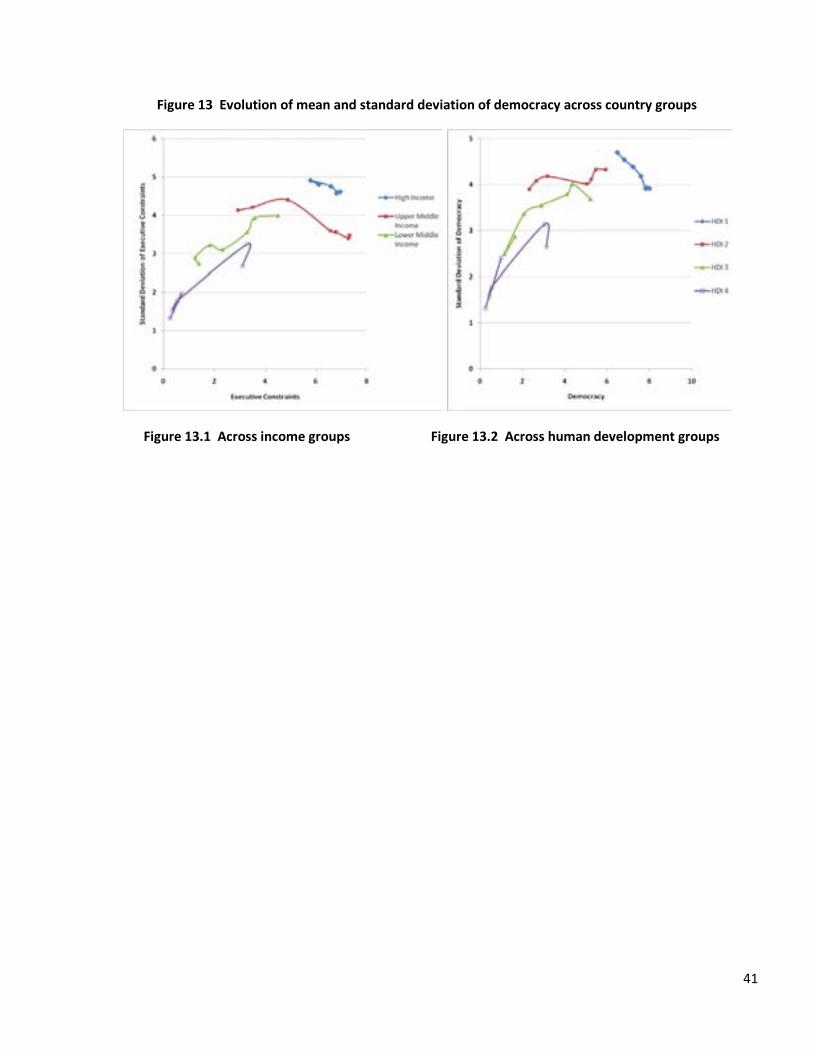
41

Figure 13 Evolution of mean and standard deviation of democracy across country groups


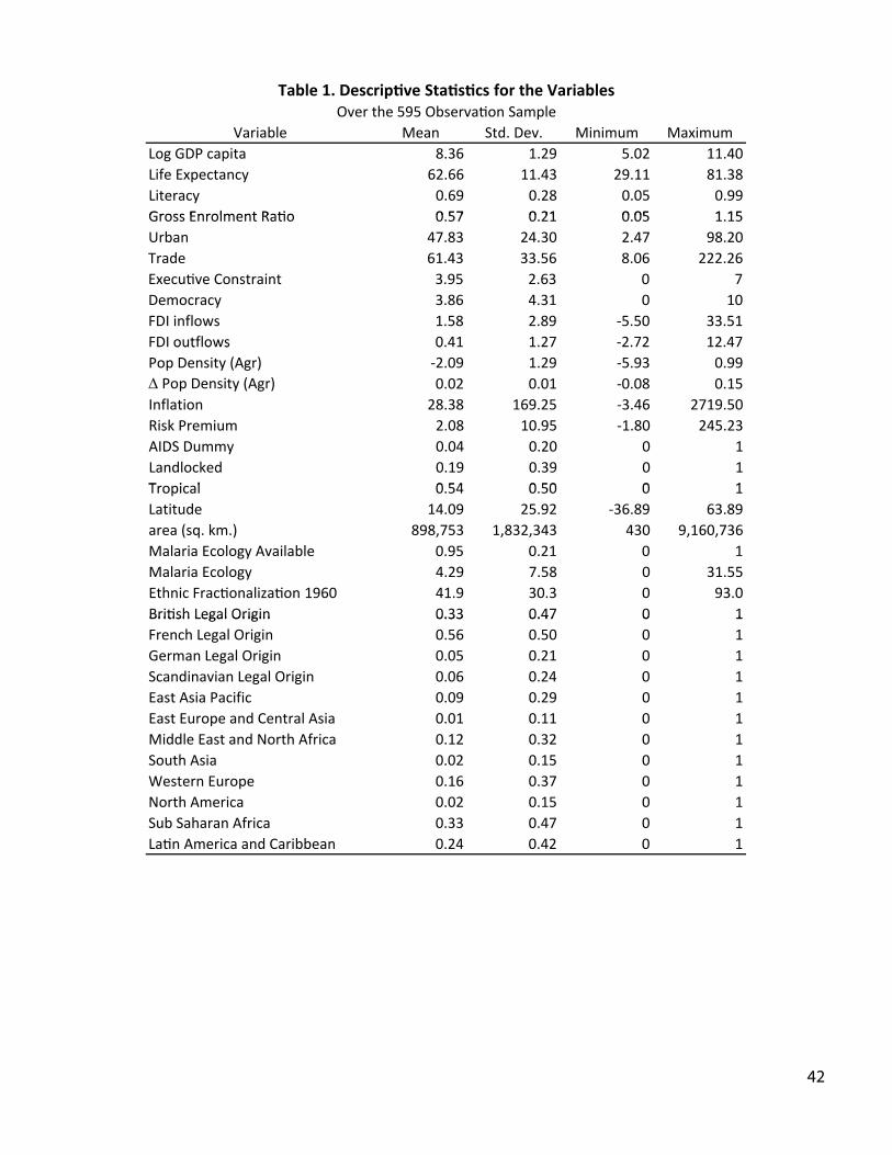
Variable Mean Std. Dev. Minimum MaximumLog GDP 04.1120.592.163.8atipacLife 83.1811.9234.1166.26ycnatcepxE

99.050.082.096.0ycaretiLGross Enrolment Ratio 0 57 0 21 0 05 1 15

Table 1. Descriptive Statistics for the VariablesOver the 595 Observation Sample

Gross Enrolment Ratio 0.57 0.21 0.05 1.1502.8974.203.4238.74nabrU62.22260.865.3334.16edarT

Executive Constraint 3.95 2.63 0 701013.468.3ycarcomeD

FDI 98.285.1swolfni -5.50 33.51FDI 72.114.0swolftuo -2.72 12.47out o s 0Pop Density (Agr) -2.09 1.29 -5.93 0.99∆ Pop Density (Agr) 0.02 0.01 -0.08 0.15

52.96183.82noitalfnI -3.46 2719.50Risk 59.0180.2muimerP -1.80 245.23AIDS 1002.040.0ymmuD

1093.091.0dekcoldnaLT i l 0 54 0 50 0 11005.045.0laciporT

29.5290.41edutitaL -36.89 63.89area (sq. 637,061,9034343,238,1357,898).mkMalaria Ecology Available 0.95 0.21 0 1Malaria 55.13085.792.4ygolocEEthnic Fractionalization 1960 41.9 30.3 0 93.0British Legal Orig 1074.033.0niBritish Legal Origin 0.33 0.47 0 1French Legal 1005.065.0nigirOGerman Legal Origin 0.05 0.21 0 1Scandinavian Legal Origin 0.06 0.24 0 1East Asia 1092.090.0cificaPEast Europe and Central Asia 0.01 0.11 0 1Middle East and North Africa 0.12 0.32 0 1

hSouth 1051.020.0aisAWestern 1073.061.0eporuENorth 1051.020.0aciremASub Saharan 1074.033.0acirfALatin America and Caribbean 0.24 0.42 0 1

42

Log GDP per Capita

Life Expectancy

LiteracyGross

Enrolment Ratio

Initial Value 0.00320*** -0.00251** -0.0119*** -0.00338**(0.00107) (0.00120) (0.000641) (0.00166)

Constant -0.0130 0.443*** 0.0143*** 0.00898***(0.00902) (0.0764) (0.000477) (0.00101)

Observations 595 595 595 595R-squared 0.015 0.007 0.369 0.007

Initial Value 0.00526*** -0.000145 -0.0129*** 0.000946(0.00113) (0.00128) (0.000676) (0.00182)

Constant -0.0302*** 0.295*** 0.0150*** 0.00650***(0.00955) (0.0812) (0.000500) (0.00110)

Observations 595 595 595 595R-squared 0.009 0.001 0.366 -0.004

Initial Value 0.00564*** -5.67e-05 -0.0139*** 0.00134*(0.000242) (0.000568) (0.000292) (0.000700)

Constant -0.0336*** 0.288*** 0.0158*** 0.00620***(0.00242) (0.0413) (0.000219) (0.000479)

Observations 595 595 595 595R-squared 0.006 0.000 0.358

Standard errors in parentheses*** p<0.01, ** p<0.05, * p<0.1

Table 2. Absolute Convergence Regressions

OLS

3SLS

IV Clustered

1970-2005

43

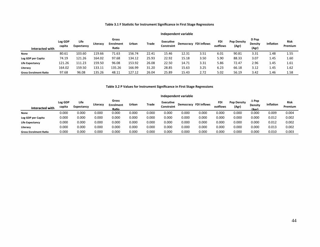
Interacted with

Log GDP capita

Life Expectancy

LiteracyGross

Enrolment Ratio

Urban TradeExecutive Constraint

Democracy FDI inflowsFDI

outflowsPop Density

(Agr)

D Pop Density

(Agr)Inflation

Risk Premium

Table 3.1 F Statistic for Instrument Significance in First Stage Regressions

Independent variable

None 80.61 103.60 119.66 71.63 156.74 22.41 15.46 12.31 3.51 6.01 90.81 3.31 1.48 1.55Log GDP per Capita 74.19 121.26 164.02 97.68 134.12 25.93 22.92 15.18 3.50 5.90 88.33 3.07 1.45 1.60Life Expectancy 121.26 111.23 159.50 96.08 153.92 26.08 22.50 14.71 3.31 5.86 72.47 2.96 1.45 1.61Literacy 164.02 159.50 133.11 135.26 166.99 31.20 28.85 15.63 3.25 6.23 66.18 3.12 1.45 1.62Gross Enrolment Ratio 97.68 96.08 135.26 48.11 127.12 26.04 25.89 15.43 2.72 5.02 56.19 3.42 1.46 1.58

Interacted with

Log GDP capita

Life Expectancy

LiteracyGross

Enrolment Ratio



outflowsPop Density

(Agr)

∆ Pop Density

(A )

InflationRisk

Premium

Table 3.2 P Values for Instrument Significance in First Stage Regressions

Independent variable

Interacted with p p yRatio

( g )(Agr)

None 0.000 0.000 0.000 0.000 0.000 0.000 0.000 0.000 0.000 0.000 0.000 0.000 0.009 0.004Log GDP per Capita 0.000 0.000 0.000 0.000 0.000 0.000 0.000 0.000 0.000 0.000 0.000 0.000 0.012 0.002Life Expectancy 0.000 0.000 0.000 0.000 0.000 0.000 0.000 0.000 0.000 0.000 0.000 0.000 0.012 0.002Literacy 0.000 0.000 0.000 0.000 0.000 0.000 0.000 0.000 0.000 0.000 0.000 0.000 0.013 0.002Gross Enrolment Ratio 0.000 0.000 0.000 0.000 0.000 0.000 0.000 0.000 0.000 0.000 0.000 0.000 0.010 0.003

44

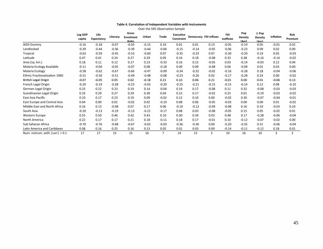
Log GDP capita

Life Expectancy

LiteracyGross

Enrolment Ratio



outflows

Pop Density

(Agr)

∆ Pop Density

(Agr)

InflationRisk

Premium

AIDS Dummy -0.16 -0.18 -0.07 -0.03 -0.15 0.10 0.01 0.01 0.13 -0.05 -0.19 0.05 -0.01 0.02Landlocked -0.39 -0.44 -0.36 -0.39 -0.44 -0.06 -0.15 -0.14 -0.05 -0.06 -0.23 0.09 0.02 0.00

Table 4. Correlation of Independent Variables with InstrumentsOver the 595 Observation Sample

Tropical -0.63 -0.59 -0.45 -0.53 -0.60 0.07 -0.35 -0.33 0.07 -0.30 -0.20 0.19 0.05 -0.03Latitude 0.47 0.41 0.24 0.27 0.29 0.05 0.16 0.18 -0.08 0.33 0.38 -0.16 -0.14 -0.02Area (sq. km.) 0.18 0.11 0.12 0.17 0.23 -0.33 0.16 0.15 -0.05 0.03 -0.14 -0.03 0.12 0.04Malaria Ecology Available -0.11 -0.04 -0.05 -0.07 0.08 -0.18 0.09 0.09 -0.08 0.06 -0.09 0.01 0.03 0.00Malaria Ecology -0.58 -0.62 -0.67 -0.66 -0.47 -0.09 -0.34 -0.32 -0.02 -0.16 -0.28 0.18 -0.04 -0.06Ethnic Fractionalization 1960 -0.51 -0.56 -0.51 -0.49 -0.48 -0.08 -0.23 -0.26 0.02 -0.17 -0.28 0.24 0.00 -0.02British Legal Origin -0 07 -0 05 0 05 0 02 -0 18 0 21 0 10 0 06 0 21 -0 01 0 00 0 01 -0 06 0 13British Legal Origin -0.07 -0.05 0.05 0.02 -0.18 0.21 0.10 0.06 0.21 -0.01 0.00 0.01 -0.06 0.13French Legal Origin -0.20 -0.19 -0.28 -0.23 -0.03 -0.20 -0.25 -0.21 -0.15 -0.15 -0.14 0.12 0.08 -0.10German Legal Origin 0.25 0.22 0.23 0.19 0.14 -0.04 0.19 0.17 -0.08 0.11 0.32 -0.08 -0.03 -0.03Scandinavian Legal Origin 0.33 0.29 0.27 0.29 0.30 0.04 0.15 0.17 -0.02 0.25 0.01 -0.19 -0.03 -0.02East Asia Pacific 0.10 0.17 0.23 0.19 0.09 -0.02 0.12 0.10 0.00 -0.02 0.30 -0.07 -0.04 -0.01East Europe and Central Asia 0.04 0.00 0.01 -0.02 0.02 -0.10 0.08 0.06 -0.05 -0.03 0.00 0.00 0.01 -0.02Middle East and North Africa 0.16 0.13 -0.08 0.07 0.17 0.06 -0.10 -0.12 -0.09 -0.08 0.16 0.10 -0.03 0.10South Asia -0.20 -0.13 -0.19 -0.13 -0.21 -0.17 0.08 0.03 -0.08 -0.05 0.15 0.05 -0.02 0.01Western Europe 0.55 0.50 0.46 0.42 0.43 0.10 0.30 0.34 0.03 0.48 0.17 -0.28 -0.06 -0.04North America 0.22 0.17 0.17 0.21 0.18 -0.11 0.18 0.17 -0.01 0.10 -0.12 -0.07 -0.02 0.00Sub Saharan Africa -0.70 -0.76 -0.68 -0.67 -0.63 -0.03 -0.36 -0.36 0.00 -0.20 -0.35 0.31 -0.06 -0.04Latin America and Caribbean 0.08 0.16 0.25 0.16 0.13 0.05 0.01 0.03 0.09 -0.14 -0.11 -0.12 0.18 0.01Num. instrum. with |corr| > 0.1 17 17 15 15 16 7 14 13 3 10 16 10 3 2

45

Method Omitted Variable: None Democracy Executive Constraints Urban

3SLS Hausman 0.99998 0.99997 0.99998 0.999983SLS Sargan 0.99975 0.98869 0.99685 0.98126IV cluster Hausman 0.0000374 0.0000516 0.00004335 0.00008158IV cluster Sargan 0.89126 0.77996 0.81095 0.64304


3SLS Hausman 0.99150 0.99163 0.99065 0.979893SLS Sargan 0.99999 0.99999 0.99937 0.37794IV cluster Hausman 0.00000110 0.00000124 0.00000108 0.00000153IV cluster Sargan 0.9865 0.9854 0.9950 0.9861


3SLS Hausman 0.00000110 0.00000124 0.00000108 0.000001533SLS Sargan 0.0000374 0.0000516 0.00004335 0.00008158IV cluster Hausman 0.0000319 0.0000254 0.0000233 3.16E-07IV cluster Sargan 0.99380 0.99772 0.96142 0.09594


3SLS Hausman 0.01020 0.00683 0.00717 0.008153SLS Sargan 0.00003193 0.00002537 0.00002327 3.158E-07IV cluster Hausman 0.000153 0.000132 0.000101 0.000007IV cluster Sargan 0.97586 0.95704 0.95094 0.85468Hausman tests with better than 1% significance in bold. Sargan tests with worse that 60% significance in bold.

for convergence estimates on rates of change of HDI components

Log GDP capita

Life Expectancy

Literacy


Table 5. P Values of Hausman and Sargan Tests

46

IV 3SLS IV 3SLS IV 3SLS IV 3SLSVariable Dependiente

Tasa de cambio de:Log GDP

per CapitaLog GDP

per CapitaLife

ExpectancyLife

Expectancy Literacy LiteracyGross

EnrolmentRatio

Gross Enrolment

Ratio-0.0113*** -0.0130** -0.00613** -0.0109* -0.00476*** -0.00163 -0.0202*** -0.0204**(0.00221) (0.00524) (0.00250) (0.00623) (0.00111) (0.00250) (0.00313) (0.00885)-0 000253 -0 000541 0 000176 -0 000306 -0 000410*** -0 000580 -0 000412 -0 000232

Table 6. Coefficients of 3SLS and Clustered Error IV Convergence EstimatesNo independent variable omitted

Dep Var X Log GDP per Capita

-0.000253 -0.000541 0.000176 -0.000306 -0.000410*** -0.000580 -0.000412 -0.000232(0.000187) (0.000634) (0.000225) (0.000597) (0.000159) (0.000395) (0.000391) (0.00107)0.0342*** 0.0380 0.0194* 0.0548* -0.0116 -0.0219 0.0295* 0.0157(0.0106) (0.0232) (0.0109) (0.0294) (0.00719) (0.0142) (0.0160) (0.0415)0.00137 -0.00478 0.00422 2.04e-05 -0.0454*** -0.0487*** -0.00636 0.0285(0.0117) (0.0318) (0.0151) (0.0381) (0.00839) (0.0180) (0.0236) (0.0632)

0.000288*** 0.000441** -3.56e-06 8.43e-05 0.000482*** 0.000500*** 0.000679*** 0.000632(6.99e-05) (0.000203) (9.89e-05) (0.000265) (7.35e-05) (0.000129) (9.59e-05) (0.000386)6.14e-05 0.000137 1.48e-05 0.000122 -7.26e-06 2.57e-05 0.000196*** 0.000139

Dep Var X Life Expectancy

Dep Var X Literacy

Dep Var X Gross Enrolment Ratio

Dep Var X Urban

6.14e-05 0.000137 1.48e-05 0.000122 -7.26e-06 2.57e-05 0.000196 0.000139(4.02e-05) (0.000111) (4.95e-05) (0.000126) (2.91e-05) (6.55e-05) (6.23e-05) (0.000171)

-0.00487*** -0.00514 -2.82e-05 -0.000495 0.00208** 0.00168 -0.00245 -0.000269(0.00145) (0.00316) (0.00188) (0.00331) (0.000888) (0.00150) (0.00242) (0.00515)

0.00395*** 0.00485* -0.00190 0.000754 -0.000784 -0.000180 0.00373* 0.000629(0.00116) (0.00250) (0.00180) (0.00283) (0.000703) (0.00137) (0.00195) (0.00430)-4.25e-05 -0.00151 0.00192 0.000885 -0.000949* -0.00108 -0.00676*** -0.00569**

(0.000796) (0.00223) (0.00118) (0.00204) (0.000554) (0.000855) (0.00158) (0.00274)-0.00274 -0.0148 0.0340*** 0.0261* -0.0313*** -0.0365*** 0.00939*** 0.0121

Dep Var X Executive Constraint

Dep Var X Democracy

Dep Var X FDI inflows

D V X FDI tfl

Dep Var X Trade

0.00274 0.0148 0.0340 0.0261 0.0313 0.0365 0.00939 0.0121(0.00361) (0.0129) (0.00695) (0.0151) (0.00862) (0.0142) (0.00248) (0.00987)-0.000529 -0.00109 0.00115** -0.000499 0.000514 0.00112 -0.00280*** -0.00346(0.000600) (0.00153) (0.000572) (0.00188) (0.000493) (0.000873) (0.000858) (0.00256)

0.0800 0.183 0.261 0.361 -0.0497 -0.0354 -0.178 -0.116(0.115) (0.279) (0.159) (0.281) (0.0546) (0.112) (0.145) (0.317)

0.000379 0.000445 0.000353 0.000485 0.000621* 0.000644 -0.00176*** -0.000650(0.000272) (0.000618) (0.000399) (0.000743) (0.000347) (0.000459) (0.000548) (0.00128)-4.46e-05 -3.57e-05 -5.03e-05*** -7.60e-05* -3.28e-05*** -1.60e-05 -0.000105*** -8.73e-05

Dep Var X Risk Premium

Dep Var X Inflation

Dep Var X FDI outflows

Dep Var X Pop Density in Agr Land (log)

Dep Var X Pop Density Growth

(3.86e-05) (5.42e-05) (1.25e-05) (4.29e-05) (9.24e-06) (3.37e-05) (1.12e-05) (7.31e-05)0.160*** 0.196*** 0.311** 0.626 0.00535*** 0.00305 0.0130*** 0.0128**(0.0270) (0.0642) (0.155) (0.397) (0.000968) (0.00198) (0.00166) (0.00538)0.00284* 0.00533 0.0224 0.0756 0.000177* 0.000241 0.000388* 0.000333(0.00146) (0.00492) (0.0192) (0.0582) (9.61e-05) (0.000239) (0.000208) (0.000526)-0.238*** -0.268 -1.702*** -3.571** 0.0667*** 0.0650*** -0.0327*** -0.0197(0.0875) (0.186) (0.638) (1.805) (0.00822) (0.0161) (0.00849) (0.0227)-0.0501 -0.00274 0.266 0.419 0.0333*** 0.0380*** 0.147*** 0.102

Dep Var X Inflation

Log GDP per Capita

Life Expectancy

Literacy

Gross Enrolment Ratio(0.106) (0.271) (1.003) (2.470) (0.00682) (0.0138) (0.0193) (0.0677)

-0.00262*** -0.00399** 0.000563 -0.00496 -0.000430***-0.000452***-0.000452*** -0.000416*(0.000638) (0.00181) (0.00681) (0.0176) (6.68e-05) (0.000108) (6.30e-05) (0.000247)-0.000457 -0.00117 -0.00192 -0.00903 3.89e-06 -1.95e-05 -0.000144*** -0.000112(0.000379) (0.000999) (0.00339) (0.00864) (2.58e-05) (5.70e-05) (4.51e-05) (0.000116)

Standard errors in parentheses, period dummies not shown*** p<0.01, ** p<0.05, * p<0.1

Urban

Trade


47

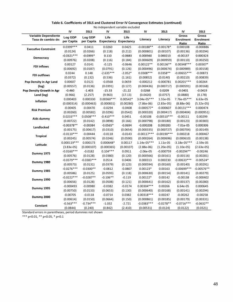
IV 3SLS IV 3SLS IV 3SLS IV 3SLSVariable Dependiente

Tasa de cambio de:Log GDP

per CapitaLog GDP

per CapitaLife

ExpectancyLife

Expectancy Literacy LiteracyGross

EnrolmentRatio

Gross Enrolment

Ratio0.0399*** 0.0411 0.0260 0.0425 -0.00188** -0.00178* 0.000108 -0.000886(0.0124) (0.0266) (0.118) (0.212) (0.000801) (0.00107) (0.00136) (0.00294)

-0 0321*** -0 0395* 0 110 -0 0683 0 000560 0 000213 -0 00137 0 000323

Table 6. Coefficients of 3SLS and Clustered Error IV Convergence Estimates (continued)No independent variable excluded

Executive Constraint

-0.0321*** -0.0395* 0.110 -0.0683 0.000560 0.000213 -0.00137 0.000323(0.00976) (0.0208) (0.116) (0.184) (0.000609) (0.000959) (0.00110) (0.00250)0.00127 0.0141 -0.125 -0.0646 0.00122** 0.00136** 0.00348*** 0.00307*

(0.00692) (0.0187) (0.0791) (0.126) (0.000496) (0.000674) (0.000989) (0.00158)0.0244 0.148 -2.635*** -2.052* 0.0308*** 0.0358** -0.00655*** -0.00873

(0.0372) (0.132) (0.536) (1.161) (0.00852) (0.0140) (0.00210) (0.00839)0.00607 0.0121 -0.0568 0.0659 -0.000212 -0.000781 0.00201*** 0.00264

(0.00557) (0.0136) (0.0391) (0.127) (0.000436) (0.000717) (0.000591) (0.00168)-0.460 -1.403 -15.33 -21.22 0.0268 0.0209 -0.0401 -0.0419

Pop Density in Agr Land (log)

Pop Density Growth in Agr

Democracy

FDI inflows

FDI outflows

-0.460 -1.403 -15.33 -21.22 0.0268 0.0209 -0.0401 -0.0419(0.966) (2.257) (9.963) (17.13) (0.0420) (0.0757) (0.0880) (0.178)

0.000403 0.000330 0.00360*** 0.00542* 3.04e-05*** 1.55e-05 7.76e-05*** 6.63e-05(0.000314) (0.000463) (0.000831) (0.00280) (7.86e-06) (2.83e-05) (8.88e-06) (5.32e-05)-0.00405 -0.00470 -0.0294 -0.0408 -0.000577* -0.000607 0.00131*** 0.000474(0.00260) (0.00582) (0.0296) (0.0542) (0.000320) (0.000417) (0.000404) (0.000951)0.0233*** 0.0508*** -0.410*** 0.0451 -0.00108 -0.00510*** -0.00111 0.00299(0.00722) (0.0142) (0.0898) (0.166) (0.000798) (0.00180) (0.00123) (0.00383)

-0.00378** -0.00384 -0.0565* -0.0694 -0.000208 0.000283 -7.01e-05 0.000306

Pop Density Growth in Agr Land (log)

Inflation

Risk Premium

Aids dummy

L dl k d0.00378 0.00384 0.0565 0.0694 0.000208 0.000283 7.01e 05 0.000306(0.00175) (0.00617) (0.0310) (0.0654) (0.000335) (0.000727) (0.000704) (0.00149)

-0.0110*** -0.00444 -0.0118 -0.0143 -0.00117*** -0.00190*** 0.000218 -0.000467(0.00245) (0.00574) (0.0246) (0.0590) (0.000264) (0.000696) (0.000610) (0.00138)

0.000119*** 0.000173 0.000648* 0.00117 1.14e-05*** 1.11e-05 -3.18e-05*** -2.59e-05(3.83e-05) (0.000107) (0.000365) (0.00107) (2.88e-06) (1.20e-05) (1.10e-05) (2.63e-05)-0.0160*** -0.0182 0.104*** 0.0911 -2.06e-05 -0.000759 -0.00294** -0.00246(0.00576) (0.0128) (0.0380) (0.120) (0.000566) (0.00161) (0.00116) (0.00281)

-0.0379*** -0.0383*** 0.0514 0.0406 0.000313 0.000230 -0.00633*** -0.00524*

Tropical

Latitude

Dummy 1975

Dummy 1980

Landlocked

(0.00573) (0.0131) (0.0379) (0.123) (0.000594) (0.00160) (0.00140) (0.00291)-0.0276*** -0.0300** -0.0812 -0.0807 0.00123* 0.00163 -0.00699*** -0.00576**(0.00586) (0.0125) (0.0593) (0.118) (0.000630) (0.00154) (0.00141) (0.00279)

-0.0222*** -0.0287** -0.106** -0.119 0.00122* 0.00142 -0.00138 -0.000402(0.00656) (0.0128) (0.0508) (0.121) (0.000641) (0.00162) (0.00137) (0.00280)-0.000493 -0.00980 -0.0382 -0.0174 0.00304*** 0.00266 6.64e-05 0.000645(0.00750) (0.0133) (0.0653) (0.130) (0.000640) (0.00168) (0.00141) (0.00294)-0.00705 -0.0118 -0.0714 0.0382 0.00318*** 0.00247 -0.00262 -0.00258

Dummy 1995

Dummy 2000

Dummy 1980

Dummy 1985

Dummy 1990

(0.00614) (0.0150) (0.0664) (0.150) (0.000861) (0.00185) (0.00179) (0.00331)-0.563*** -0.734*** -1.032 -2.721 -0.0383*** -0.0278** -0.0716*** -0.0632**(0.0844) (0.240) (0.842) (2.410) (0.00531) (0.0124) (0.0122) (0.0321)

Standard errors in parentheses, period dummies not shown*** p<0.01, ** p<0.05, * p<0.1

Dummy 2000

Constant

48

Interacted VariablesLog GDP per Capita (-)*** (-)*** (-)*** (-)*** (-)** (-)** (-)** (-)*** (-)*** (-)*** (-)*** (-)*** (-)*** (-)*** (-)***

Life Expectancy (-)*** (-)*** (-)***Literacy (+)*** (+)*** (+)*** (+)* (+)* (+)* (+)** (-)** (-)*** (+)*

Log GDP per Capita Life Expectancy Literacy Gross Enrolment Ratio

Table 7. Sign and Significance Patterns for Coefficients of Clustered Error IV Convergence EstimatesOmitted Variables Marked in Gray

y ( ) ( ) ( ) ( ) ( ) ( ) ( ) ( ) ( ) ( )Gross Enrolment Ratio (***)+( -)*** (-)*** (-)*** (-)***

Urban ***)+(***)+(***)+(***)+(***)+(***)+(***)+(***)+(***)+(Trade (+)*** (+)* (+)** (+)***

Executive Constraint (-)*** (-)*** (-)*** (+)** (+)*** (+)*** (+)*Democracy (+)*** (+)*** (- **)+(*)+(***)+(**)FDI inflows (+)* (+)** (+)* (-)* (-)* (-)* (-)*** (-)*** (-)*** (-)**( ) ( ) ( ) ( ) ( ) ( ) ( ) ( ) ( ) ( )

FDI outflows (+)*** (+)*** (+)*** (+)*** (-)*** (-)*** (-)*** (-)*** (+)*** (+)*** (+)*** (+)**Pop Density in Agr Land (log) (-)** (+)** (+)** (+)* (+)** (+)** (-)*** (-)*** (-)*** (-)***

Pop Density Growth (+)*** (+)** (+)* (-)* (-)** (-)* (-)* (-)Risk Premium (**)+(*)+(**)+(**)+(**)+( -)*** (-)** (-)** (-)***

Inflation (-)*** (-)*** (-)*** (-)*** (-)*** (-)*** (-)*** (-)*** (-)*** (-)*** (-)***Non-Interacted Controls

AIDS dummy (+)*** (+)*** (+)*** (+)*** (-)*** (-)*** (-)*** (- (***) -)Landlocked (- (**) -)* (- **)+(**)

Tropical (-)*** (-)*** (-)*** (- (***) -)*** (-)*** (-)*** (-)*** (+)*Latitude (+)*** (+)*** (+)*** (+)*** (+)* (+)** (+)* (+)** (+)*** (+)*** (+)*** (+)* (-)*** (-)** (-)** (-)***

Significance indicated as follows: *** p<0.01, ** p<0.05, * p<0.1

49

q10 q20 q30 q40 q50 q60* q70 q80 q90

0.0551*** 0.0438*** 0.0353*** 0.0369*** 0.0407*** 0.0348*** 0.0442*** 0.0495*** 0.0542***(0.00677) (0.00790) (0.00885) (0.00615) (0.00576) (0.00576) (0.00672) (0.00920) (0.0114)1.225*** 1.076*** 0.878*** 0.984*** 0.795*** 0.797*** 0.603*** 0.517** 0.779***(0.292) (0.302) (0.328) (0.226) (0.204) (0.193) (0.212) (0.259) (0.292)

-0.976** -0.514 -0.266 -0.0562 0.0777 0.155 0.583* 1.232*** 0.705(0.412) (0.416) (0.475) (0.330) (0.307) (0.295) (0.329) (0.434) (0.480)

0.0163*** 0.0186*** 0.0209*** 0.0185*** 0.0208*** 0.0225*** 0.0184*** 0.0116*** 0.00584(0.00198) (0.00212) (0.00228) (0.00163) (0.00156) (0.00157) (0.00188) (0.00278) (0.00375)

-0.00173** 0.000368 0.00244** 0.000760 0.000883 0.00113 0.00121 0.00198 0.00400**(0.000875) (0.00105) (0.00111) (0.000784) (0.000763) (0.000771) (0.000892) (0.00125) (0.00155)0.143*** 0.102*** 0.0875*** 0.0784*** 0.101*** 0.0997*** 0.0993*** 0.0727** 0.101***(0.0161) (0.0198) (0.0249) (0.0186) (0.0185) (0.0187) (0.0218) (0.0307) (0.0366)

-0.0675*** -0.0354** -0.0226 -0.0169 -0.0309** -0.0288** -0.0451*** -0.0619*** -0.0789***(0.0122) (0.0143) (0.0172) (0.0128) (0.0128) (0.0129) (0.0150) (0.0204) (0.0247)

-0.0521*** -0.0803*** -0.0415** -0.0230* -0.0324*** -0.0452*** -0.0468*** -0.0282 -0.0208(0.0155) (0.0169) (0.0180) (0.0124) (0.0117) (0.0119) (0.0146) (0.0212) (0.0246)0.173*** 0.124*** 0.0665* 0.0192 0.0303 0.0200 0.00366 -0.0261 -0.0834(0.0252) (0.0316) (0.0368) (0.0249) (0.0253) (0.0253) (0.0311) (0.0424) (0.0523)

-0.101*** -0.0535*** -0.0444* -0.0170 -0.0233 0.00303 -0.00858 0.00306 -0.0103(0.0187) (0.0204) (0.0228) (0.0165) (0.0156) (0.0158) (0.0183) (0.0252) (0.0295)

-10.41*** -11.90*** -0.759 2.625 8.179*** 9.211*** 8.750*** 6.976* 8.032(3.399) (3.714) (3.873) (2.743) (2.549) (2.499) (2.898) (4.034) (5.151)

-0.00132 -0.0110*** -0.00836* -0.0112*** -0.0165*** -0.0196*** -0.0189*** -0.0123*** -0.00355(0.00327) (0.00401) (0.00454) (0.00357) (0.00352) (0.00342) (0.00369) (0.00418) (0.00528)

0.00119*** 0.000644* 0.000358 0.000127 -3.53e-05 2.44e-05 0.000115 0.000160 0.000215(0.000297) (0.000344) (0.000391) (0.000277) (0.000269) (0.000269) (0.000318) (0.000433) (0.000528)

0.246** 0.0120 -0.137 -0.183* -0.0989 -0.0930 0.160 0.270* 0.155(0.106) (0.128) (0.143) (0.0999) (0.0917) (0.0898) (0.106) (0.140) (0.170)

0.225*** 0.220*** 0.132* 0.163*** 0.144*** 0.139*** 0.120** 0.164** 0.114(0.0646) (0.0713) (0.0771) (0.0540) (0.0524) (0.0522) (0.0607) (0.0816) (0.0944)0.1000 0.120 -0.0480 -0.0993* -0.0863 -0.0803 -0.0841 -0.180** -0.374***

(0.0712) (0.0768) (0.0840) (0.0577) (0.0536) (0.0504) (0.0570) (0.0750) (0.0931)0.0121*** 0.00961*** 0.00984*** 0.0100*** 0.00672*** 0.00612*** 0.00490*** 0.00405*** 0.00402***(0.00105) (0.00110) (0.00127) (0.000923) (0.000875) (0.000842) (0.000961) (0.00120) (0.00147)2.727*** 3.503*** 3.877*** 3.960*** 3.698*** 4.066*** 3.742*** 3.805*** 4.057***(0.310) (0.371) (0.421) (0.302) (0.290) (0.293) (0.345) (0.474) (0.629)

Observations 595 595 595 595 595 595 595 595 595Standard errors in parentheses*** p<0.01, ** p<0.05, * p<0.1

Literacy

Gross Enrolment RatioUrban

Tropical

Latitude

Trade

Log GDP per Capita

Life Expectancy

Agric Dens Growth

Risk Premium

Inflation

Democracy

Aids Dummy

Landlocked

Constant


FDI inflows

FDI outflows

Agric Density

Instrumented Quantile RegressionTable 8.1 Log GDP per Capita

50

q10 q20 q30 q40 q50 q60 q70 q80 q902.111** 2.968*** 2.077*** 1.867*** 1.679*** 1.761*** 2.225*** 1.992*** 2.047***(0.902) (0.452) (0.393) (0.341) (0.478) (0.464) (0.458) (0.284) (0.315)

16.22*** 14.10*** 16.26*** 14.70*** 14.48*** 12.14*** 10.76*** 11.01*** 8.456***(3.002) (1.760) (1.573) (1.517) (2.245) (2.352) (2.394) (1.747) (2.088)-2.101 -1.241 -0.708 1.972 3.692 5.099 6.856* 10.88*** 18.05***(4.329) (2.530) (2.378) (2.328) (3.457) (3.541) (3.552) (2.503) (2.847)0.0480 0.0378** 0.0606*** 0.0723*** 0.0817*** 0.100*** 0.0867*** 0.0764*** 0.0512***

(0.0337) (0.0170) (0.0148) (0.0131) (0.0186) (0.0181) (0.0182) (0.0122) (0.0138)0.00790 0.0186** 0.0248*** 0.0328*** 0.0299*** 0.0241*** 0.0271*** 0.0304*** 0.0259***(0.0127) (0.00760) (0.00669) (0.00590) (0.00850) (0.00840) (0.00834) (0.00548) (0.00593)

-1.713*** -1.228*** -1.054*** -0.774*** -0.661*** -0.782*** -0.687*** -0.877*** -0.474***(0.287) (0.164) (0.153) (0.144) (0.206) (0.207) (0.203) (0.134) (0.142)

1.597*** 1.151*** 1.044*** 0.852*** 0.683*** 0.752*** 0.691*** 0.668*** 0.399***(0.198) (0.112) (0.0983) (0.0928) (0.134) (0.135) (0.134) (0.0908) (0.102)-0.0523 -0.106 -0.0333 -0.0919 -0.0157 0.131 0.242** 0.273*** 0.367***(0.205) (0.130) (0.120) (0.105) (0.136) (0.125) (0.117) (0.0767) (0.0737)-0.161 -0.228 -0.474** -0.547*** -0.674** -0.884*** -0.990*** -1.220*** -1.202***(0.338) (0.277) (0.233) (0.209) (0.286) (0.277) (0.277) (0.201) (0.235)0.459 0.513*** 0.487*** 0.450*** 0.539*** 0.750*** 0.647*** 0.660*** 0.375***

(0.294) (0.160) (0.139) (0.125) (0.176) (0.175) (0.170) (0.111) (0.105)-150.3*** -108.2*** -87.67*** -82.61*** -65.10** -56.68** -45.74* -28.57 -35.30*

(44.94) (26.67) (22.27) (20.25) (28.26) (27.88) (26.76) (18.13) (19.21)0.0871* 0.0556 0.0205 -0.00300 -0.0271 -0.0518 -0.0514 -0.0509** -0.0283(0.0519) (0.0421) (0.0323) (0.0297) (0.0405) (0.0390) (0.0320) (0.0205) (0.0219)-0.00578 -0.00574* -0.00383 -0.00402* -0.00500 -0.00528* -0.00834*** -0.00803*** -0.0103***(0.00543) (0.00301) (0.00253) (0.00226) (0.00305) (0.00288) (0.00269) (0.00163) (0.00174)-5.242*** -5.565*** -4.712*** -3.883*** -4.422*** -4.226*** -5.140*** -5.187*** -5.357***

(1.719) (0.888) (0.820) (0.722) (1.032) (0.960) (0.966) (0.638) (0.745)-3.957*** -2.508*** -2.765*** -1.953*** -1.828*** -0.646 0.0977 0.607* 0.558

(0.966) (0.534) (0.457) (0.412) (0.587) (0.562) (0.550) (0.365) (0.429)-3.058*** -3.027*** -2.560*** -2.030*** -1.938*** -1.621*** -1.316** -1.659*** -1.609***

(0.837) (0.451) (0.410) (0.401) (0.595) (0.595) (0.629) (0.445) (0.525)-0.00367 -0.00553 0.00608 0.00824 0.0140 0.0238** 0.0135 0.0136** 0.0211***(0.0207) (0.0104) (0.00869) (0.00775) (0.0105) (0.00988) (0.00916) (0.00564) (0.00517)35.19*** 29.32*** 33.42*** 33.74*** 35.01*** 35.42*** 32.25*** 33.68*** 32.19***(4.903) (2.780) (2.410) (2.148) (3.115) (3.102) (3.138) (2.035) (2.366)


Trade

Log GDP per Capita

Life Expectancy

Literacy



FDI inflows

FDI outflows

Agric Density

Agric Dens Growth

Inflation

Risk Premium

Constant

Instrumented Quantile RegressionTable 8.2 Life Expectancy

Aids Dummy

Landlocked

Tropical

Latitude

51

q10 q20 q30 q40 q50 q60 q70 q80 q900.0417*** 0.0370** 0.0372** 0.0413*** 0.0399*** 0.0402** 0.0329*** 0.0192** 0.0243**(0.0159) (0.0163) (0.0151) (0.0125) (0.0127) (0.0156) (0.0120) (0.00911) (0.0105)0.00181 0.00724*** 0.00703*** 0.00951*** 0.0112*** 0.0111*** 0.0119*** 0.0123*** 0.0107***

(0.00202) (0.00185) (0.00180) (0.00154) (0.00166) (0.00221) (0.00192) (0.00160) (0.00210)

1.117*** 1.028*** 1.113*** 0.989*** 0.948*** 0.955*** 0.810*** 0.697*** 0.554***(0.0811) (0.0861) (0.0795) (0.0676) (0.0705) (0.0919) (0.0800) (0.0648) (0.0807)

-3.29e-05 -0.000595 -0.00132** -0.00145*** -0.00221*** -0.00215*** -0.00217*** -0.00155*** -0.00132***(0.000549) (0.000563) (0.000557) (0.000478) (0.000481) (0.000604) (0.000458) (0.000354) (0.000443)

-0.00130*** -0.00114*** -0.000996*** -0.00100*** -0.000943*** -0.000666** -6.60e-05 0.000289 0.000253(0.000253) (0.000282) (0.000257) (0.000213) (0.000219) (0.000277) (0.000224) (0.000179) (0.000234)

0.00685 0.0109 0.0111* 0.0126** 0.00806 0.0131* 0.0180*** 0.0176*** 0.0116**(0.00746) (0.00727) (0.00656) (0.00548) (0.00545) (0.00685) (0.00564) (0.00439) (0.00500)-0.00228 -0.00506 -0.00735 -0.0120*** -0.0121*** -0.0158*** -0.0176*** -0.0162*** -0.0122***(0.00510) (0.00501) (0.00449) (0.00372) (0.00372) (0.00473) (0.00397) (0.00315) (0.00381)-0.00390 -0.00756* -0.0124*** -0.00421 -0.00324 -0.00210 -0.00424 -0.00624*** -0.00283(0.00379) (0.00385) (0.00360) (0.00314) (0.00334) (0.00436) (0.00303) (0.00231) (0.00267)0.0148* 0.000911 0.00556 -0.000975 0.00316 -0.000901 -0.00593 -0.00385 -0.00455

(0.00830) (0.00790) (0.00814) (0.00713) (0.00731) (0.00933) (0.00778) (0.00536) (0.00625)0.0199*** 0.0107 0.00249 0.00483 -0.00203 -0.00478 -0.00508 -0.00313 -0.000304(0.00669) (0.00691) (0.00577) (0.00458) (0.00454) (0.00559) (0.00462) (0.00362) (0.00429)

-0.181 0.0363 -1.172 -1.401** -2.130*** -1.520* -3.672*** -4.264*** -4.673***(0.832) (0.939) (0.827) (0.696) (0.721) (0.910) (0.737) (0.603) (0.752)

-0.000440 -0.000336 0.000533 0.000721 0.00177* 0.000922 3.10e-05 8.83e-05 -0.000257(0.00107) (0.00108) (0.00102) (0.000963) (0.00104) (0.00130) (0.00116) (0.000813) (0.00129)-6.08e-05 -0.000129 -0.000205** -0.000165** -0.000124 -0.000137 -7.20e-05 -3.05e-05 -6.31e-06

(0.000132) (0.000112) (9.64e-05) (7.88e-05) (7.82e-05) (9.51e-05) (7.84e-05) (6.24e-05) (7.14e-05)0.0208 0.0587* 0.0255 0.0218 0.0112 0.0100 -0.00794 -0.00208 -0.0299

(0.0201) (0.0319) (0.0315) (0.0265) (0.0265) (0.0342) (0.0281) (0.0223) (0.0283)0.0455*** 0.0396** 0.0338** 0.0526*** 0.0424*** 0.0445** 0.0311* 0.0257** 0.0245(0.0174) (0.0179) (0.0168) (0.0143) (0.0150) (0.0195) (0.0163) (0.0125) (0.0160)0.144*** 0.131*** 0.116*** 0.0931*** 0.0654*** 0.0552*** 0.0449*** 0.0472*** 0.0305**(0.0184) (0.0200) (0.0185) (0.0149) (0.0146) (0.0177) (0.0149) (0.0120) (0.0147)

-0.00109*** -0.000857** -0.00106*** -0.00120*** -0.00123*** -0.000978*** -0.000723*** -0.000635*** -0.000585**(0.000360) (0.000348) (0.000319) (0.000257) (0.000262) (0.000325) (0.000276) (0.000224) (0.000271)-0.504*** -0.702*** -0.653*** -0.713*** -0.698*** -0.714*** -0.584*** -0.437*** -0.256**(0.0965) (0.117) (0.104) (0.0859) (0.0873) (0.110) (0.0884) (0.0718) (0.0998)



FDI inflows

FDI outflows

Agric Density

Agric Dens Growth

Inflation

Log GDP per Capita

Life Expectancy

Literacy


Trade

Risk Premium

Constant

Latitude

Instrumented Quantile RegressionTable 8.3 Literacy

Aids Dummy

Landlocked

Tropical

52

q10 q20 q30 q40 q50 q60 q70 q80 q900.0227*** 0.0213*** 0.0153** 0.00485 -0.00184 -0.00295 -0.00487 0.00571 0.0107(0.00833) (0.00804) (0.00714) (0.00885) (0.0111) (0.00947) (0.0123) (0.0143) (0.0124)0.00253** -3.56e-06 -0.000575 0.00106 0.000896 0.00265** 0.00412** 0.00423** 0.00615***(0.00105) (0.00122) (0.000988) (0.00123) (0.00147) (0.00127) (0.00161) (0.00177) (0.00188)0.322*** 0.385*** 0.418*** 0.428*** 0.460*** 0.454*** 0.454*** 0.463*** 0.431***(0.0323) (0.0311) (0.0265) (0.0333) (0.0402) (0.0354) (0.0462) (0.0533) (0.0564)

0.00243*** 0.00205*** 0.00181*** 0.00137*** 0.00156*** 0.000869** 0.000295 -0.000672 -0.00128***(0.000306) (0.000296) (0.000272) (0.000336) (0.000409) (0.000345) (0.000450) (0.000513) (0.000447)

0.000728*** 0.000537*** 0.000573*** 0.000327** 0.000366** 0.000304* 0.000179 1.82e-05 -0.000143(0.000174) (0.000147) (0.000123) (0.000151) (0.000186) (0.000158) (0.000200) (0.000238) (0.000221)-0.00546 -0.00236 -0.00177 -0.00429 -0.00554 -0.00895** -0.00489 -0.00607 0.00651(0.00430) (0.00398) (0.00324) (0.00388) (0.00462) (0.00392) (0.00493) (0.00594) (0.00543)0.00600** 0.00440 0.00525** 0.00595** 0.00701** 0.00754*** 0.00480 0.00529 -0.00662*(0.00303) (0.00275) (0.00220) (0.00265) (0.00313) (0.00264) (0.00325) (0.00376) (0.00347)

-0.00780** 0.00434 0.00642*** 0.00874*** 0.00922*** 0.00829*** 0.0107*** 0.0105*** 0.0165***(0.00305) (0.00275) (0.00214) (0.00249) (0.00287) (0.00235) (0.00278) (0.00310) (0.00291)0.00609 -0.00358 -0.00419 0.00125 0.00163 0.00948* 0.0215*** 0.0232*** 0.0361***

(0.00628) (0.00596) (0.00471) (0.00530) (0.00607) (0.00504) (0.00594) (0.00628) (0.00640)0.00185 0.0116*** 0.00947*** 0.00955*** 0.0102*** 0.00711** 0.00393 0.00156 0.00191

(0.00370) (0.00308) (0.00252) (0.00312) (0.00379) (0.00338) (0.00435) (0.00535) (0.00592)1.590*** 0.303 -0.185 0.564 1.189* 1.615*** 2.502*** 3.173*** 3.660***(0.513) (0.513) (0.417) (0.512) (0.610) (0.515) (0.658) (0.775) (0.689)

-0.000743 -0.000753 -0.000682 -0.000791 -0.00101 -0.000137 -0.000452 0.00114 0.00381***(0.000949) (0.000863) (0.000665) (0.000773) (0.000868) (0.000664) (0.000780) (0.000839) (0.000768)

0.000176*** 0.000193*** 0.000233*** 0.000224*** 0.000207*** 0.000185*** 0.000212*** 0.000221** 0.000230***(4.41e-05) (4.58e-05) (3.73e-05) (4.90e-05) (6.33e-05) (5.74e-05) (7.47e-05) (8.80e-05) (8.41e-05)0.0714*** 0.0928*** 0.0784*** 0.0730*** 0.0647*** 0.0507*** 0.0464* 0.0426 0.0322(0.0192) (0.0178) (0.0145) (0.0184) (0.0221) (0.0188) (0.0244) (0.0265) (0.0237)0.000311 0.00264 -0.0139 -0.0228** -0.0276** -0.0308*** -0.0265* -0.0309** -0.0272(0.0119) (0.0108) (0.00860) (0.0106) (0.0126) (0.0106) (0.0139) (0.0151) (0.0169)-0.00927 -0.0383*** -0.0473*** -0.0508*** -0.0400*** -0.0441*** -0.0414*** -0.0447*** -0.0293**(0.00955) (0.00967) (0.00817) (0.0102) (0.0126) (0.0112) (0.0143) (0.0163) (0.0129)-6.64e-05 0.000114 0.000219 0.000134 0.000139 -2.98e-05 -0.000128 8.50e-06 0.000156

(0.000229) (0.000204) (0.000163) (0.000192) (0.000228) (0.000194) (0.000249) (0.000283) (0.000285)-0.273*** -0.0484 0.0458 0.0751 0.111 0.0728 0.0167 -0.0171 -0.129(0.0626) (0.0591) (0.0506) (0.0641) (0.0815) (0.0708) (0.0926) (0.106) (0.102)


Agric Dens Growth

Inflation

Risk Premium

Constant

Aids Dummy

Log GDP per Capita

Life Expectancy

Literacy


Trade


FDI inflows

FDI outflows

Instrumented Quantile RegressionTable 8.4 Gross Enrolment Ratio

Agric Density

Landlocked

Tropical

Latitude

53

TotalSignificance

Positive Negative ScoreDivergent Convergent (sign

independent)Log GDP per Capita ( )*** ( )** ( )*** ( )*** 9 9 3 0 11 21 0 32

Sum of Stars for

Significant Coefficients

Table 9. Summary and Comparison of Convergence and Quantile Estimates

Coefficients

Log GDP per Capita

Life Expect-ancy Literacy

Gross Enrolment

Ratio

Log GDP per Capita

Life Expect-ancy Literacy

Gross Enrolment

Ratio

Convergence EstimateClustered Error IV, no Variable Omitted

Quantile Level EstimatesIndependent Variables Instrumented

Summary of Significance in Quantile Estimates

Summary of Significance in Convergence Estimates

Log GDP per Capita (-)*** (-)** (-)*** (-)*** 9 9 3 0 11 21 0 32Life Expectancy (-)*** 9 8 5 0 3 22 0 25

Literacy (+)*** (+)* (+)* 9 9 9 5 0 27 0 32Gross Enrolment Ratio (- 2130920***) -1 16

Urban (+)*** (+)*** (+)*** 8 8 -7 5 9 0 22 -8 39Trade (+)*** 1 8 -6 5 3 0 15 -7 25

Executive Constraints (-)*** (+)** 9 -9 4 -1 2 3 13 -10 28Democracy (+)*** (+)* -7 9 -6 5 4 0 14 -13 31Democracy (+) (+) -7 9 -6 5 4 0 14 -13 31FDI inflows (-)* (-)*** -6 3 -3 6 0 4 10 -10 24

FDI outflows (+)*** (-)*** (+)*** 2 -7 0 3 6 3 5 -7 21Pop Density in Agr Land (log) (+)** (-)*** -2 8 1 5 2 3 14 -2 21

Pop Density Growth 1 -6 -5 5 0 0 8 -13 21Low Risk Premium (-)* (+)*** -1 3 2 -9 3 1 7 -1 12

Low Inflation (+)*** (+)*** (+)*** 6 1 0 -1 9 0 5 -10 24

54

Date post:	25-Oct-2021
Category:	Documents
Upload:	others
View:	1 times
Download:	0 times

Human Development Research Paper 2010/20 Divergences and ...

Documents