Page 1
Human Powered Vehicle
Challenge
By
Matt Gerlich, Alex Hawley, Phillip Kinsley,
Heather Kutz, Kevin Montoya, Erik Nelson
Team 9
Engineering Analysis Document
Submitted towards partial fulfillment of the requirements for
Mechanical Engineering Design I – Fall 2013
Department of Mechanical Engineering
Northern Arizona University Flagstaff, AZ 86011
Page 2
1
TABLE OF CONTENTS
1.0 INTRODUCTION .................................................................................................................... 1
2.0 PROJECT DESCRIPTION ....................................................................................................... 1
3.0 ANALYSIS ............................................................................................................................... 2
3.1 FRAME ................................................................................................................................. 2
3.2 ERGONOMICS .................................................................................................................. 10
3.3 FAIRING ............................................................................................................................. 12
3.4 STEERING.......................................................................................................................... 14
3.5 DRIVETRIAN .................................................................................................................... 19
3.6 INNOVATION.................................................................................................................... 21
4.0 PROJECT SCHEDULE .......................................................................................................... 27
5.0 CONCLUSION ....................................................................................................................... 27
6.0 REFERENCES ....................................................................................................................... 28
7.0 APPENDIX ............................................................................................................................. 29
1.0 INTRODUCTION
For the 2014 Human Powered Vehicle Challenge (HPVC) Team 9 will design, analyze,
and construct a vehicle that meets the requirements given by the American Society of
Mechanical Engineers (ASME) and the project’s client, Perry Wood. To analyze the vehicle, the
project was divided into six subsections. These sections include: frame, fairing, steering,
drivetrain, ergonomics, and innovation. For each subsection a set of analysis was computed
either mathematically or numerically. Each analysis task completed will be explained in detail
with the results presented. This paper will also give an update on the project’s overall progress.
2.0 PROJECT DESCRIPTION
Team 9 will design and build a human powered vehicle to compete in the HPVC, held by
ASME. The competition consists of a design event, a sprint or drag event, an endurance race, and
an innovation presentation. The sponsors for this project are Perry Wood, the NAU ASME
advisor, and ASME. A goal statement was generated that states the team will “Design a human
powered vehicle that can function as an alternative form of transportation.” This provides the
team a large scope while brainstorming ideas within their sections. A few objectives the team
has for the vehicle includes: speed, aerodynamics, and maneuverability.
Page 3
2
3.0 ANALYSIS
3.1 FRAME
The frame section of the analysis was broken into three separate sections: the main center
tube, the outriggers, and the roll bar. Bending resistances were examined for the center tube
because they were deemed important. The outriggers and the roll bar were both analyzed for
stresses and deflections. Along with the above analysis, all the weights were compared to find
the most optimal strength to weight ratio for each part.
Initially five different configurations were analyzed by hand. These configurations
include: 2” diameter aluminum with 0.125” thickness, 1.75” diameter aluminum with 0.125”
thickness, 1.5”x1.5” square aluminum with 0.125” thickness, 2”x1” rectangular aluminum with
0.125” thickness, and 1.5” diameter steel with 0.058” thickness, which was used as a baseline
comparison because it was used on NAU’s Human Powered Vehicle in the past. All of the
aluminum being analyzed is 6061 T6 and the steel is 4130.
The first analysis task was to find resistance to deflection for the center tube for each
configuration. The frame was simplified to a simply supported beam with an applied load to the
top. From this, a free body diagram was constructed, as seen in Figure 1. The deflection for this
case can be found using the following equation [1]:
(1)
Where:
F= applied force [lb]
b= distance from B to force [in]
x= distance from A to force [in]
L= length of beam [in]
E= modulus of elasticity [ksi]
I= moment of inertia [in4]
Figure 1- Frame Free Body Diagram
Page 4
3
The modulus of elasticity for 6061 T6 aluminum is 10,400 ksi, and for 4130, the modulus
of elasticity is 29,000 ksi [2]. The moment of inertia was found for the rectangular and square
cross sections using the following equation:
(2)
Where:
b1= outside base [in]
b2= inner base [in]
h1= outer height [in]
h2= inner height [in]
To find the moment of inertia for the circular cross sections the following equation was used:
(3)
Where:
do= outer diameter [in]
di= inner diameter [in]
The same deflection calculations were performed on the outriggers. These were simplified into a
cantilever beam with an applied load to the end. The free body diagram for this can be seen
below:
Figure 2- Outrigger Free Body Diagram
Page 5
4
The deflection for this scenario is given by the following equation:
(4)
Where:
P= Fcos(15°) [lbs]
In addition to this, the bending stresses on the outriggers also needed to be calculated. To
accomplish this, the following equation was used:
(5)
Where:
c= distance from neutral axis to extreme fiber [in]
M= moment [lb-in]
Stress concentrations were also taken into account for the outrigger connection to the frame. To
find the stress concentration the following equations were used:
(6)
Where:
q= notch sensitivity
kt= theoretical stress concentration factor
(7)
Kt and q were approximated for aluminum using tables [2]. Kf was found to be 1.54 for the
square geometry and 1.45 for the round geometry.
The results from these calculations are given in Table 1 below. The force applied on the
main tube was 600lb, and the force on the edge of the outriggers was 275lb, measured from
accelerometer tests, seen in Appendix A. The deflections were also calculated for a lateral load
applied in the z-direction of the material. The lateral load for the main tube was 300lb and the
lateral load for the outriggers was 100lb.
Page 6
5
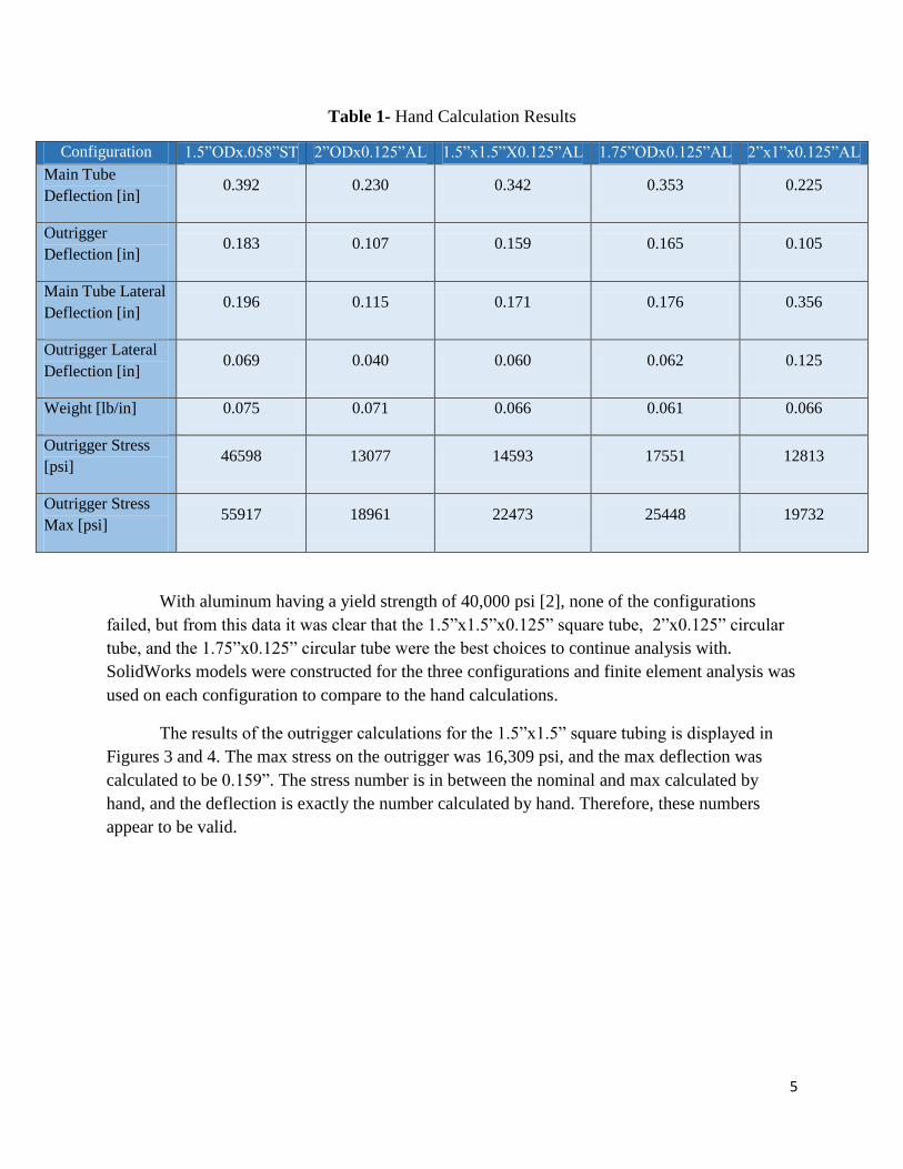
Table 1- Hand Calculation Results
Configuration 1.5”ODx.058”ST 2”ODx0.125”AL 1.5”x1.5”X0.125”AL 1.75”ODx0.125”AL 2”x1”x0.125”AL
Main Tube
Deflection [in] 0.392 0.230 0.342 0.353 0.225
Outrigger
Deflection [in] 0.183 0.107 0.159 0.165 0.105
Main Tube Lateral
Deflection [in] 0.196 0.115 0.171 0.176 0.356
Outrigger Lateral
Deflection [in] 0.069 0.040 0.060 0.062 0.125
Weight [lb/in] 0.075 0.071 0.066 0.061 0.066
Outrigger Stress
[psi] 46598 13077 14593 17551 12813
Outrigger Stress
Max [psi] 55917 18961 22473 25448 19732
With aluminum having a yield strength of 40,000 psi [2], none of the configurations
failed, but from this data it was clear that the 1.5”x1.5”x0.125” square tube, 2”x0.125” circular
tube, and the 1.75”x0.125” circular tube were the best choices to continue analysis with.
SolidWorks models were constructed for the three configurations and finite element analysis was
used on each configuration to compare to the hand calculations.
The results of the outrigger calculations for the 1.5”x1.5” square tubing is displayed in
Figures 3 and 4. The max stress on the outrigger was 16,309 psi, and the max deflection was
calculated to be 0.159”. The stress number is in between the nominal and max calculated by
hand, and the deflection is exactly the number calculated by hand. Therefore, these numbers
appear to be valid.
Page 7
6
Figure 3- Square Outrigger Stress
Figure 4- Square Outrigger Deflection
The finite element analysis results for the 1.75” circular tubing outriggers is displayed in
Figures 5 and 6. The max stress the outrigger experienced in this test was 21,897 psi, and the
maximum deflection was 0.139”. The stress, again, fell between the nominal and maximum
calculated values, and the deflection was slightly less than the value calculated by hand.
Page 8
7
Figure 5- Circular Outrigger Stress
Figure 6- Circular Outrigger Deflection
The roll bar was also tested in three separate loading configurations: the max driving load
of 225lb at the wheel from the accelerometer readings, 600lb top load, and 300lb side load as per
the competition requirements.
Page 9
8
The 225lb load at the wheel test can be seen in Figure 7. This test resulted in a maximum
stress of 13,600 psi.
Figure 7- Driving Load Roll Bar Stress
The next test was the 600lb top load applied at an angle of 12° from vertical. The
maximum stress experienced was 25,926psi, and the overall deformation was 0.607”, which is
well below the competition requirements of 2”. This deflection can be seen in Figure 8 below:
Figure 8-Top Load Roll Bar Deflection
Page 10
9
With the 300lb load applied at shoulder height, the roll bar experienced a maximum
stress of 20,171 psi and a maximum deflection of 0.511”, again below the competition
requirement of less than 1.5”. This deflection can be seen in the Figure 9 below:
Figure 9- Side Load Roll Bar Deflection
A summary of the comparisons between the finite element analysis and the hand
calculations is given below in Table 2. Since several assumptions were made to perform the
calculations, and all of these results are close to what was calculated, these results appear to be
accurate.
Table 2- FEA vs. Calculated Results
Configuration 1.5x1.5X0.125AL 1.75ODx0.125AL
Calculated Deflection [in] 0.159 0.165
FEA Deflection [in] 0.159 0.139
Calculated Nominal Stress
[psi] 14593 17551
Calculated Max Stress [psi] 22473 25448
FEA Stress [psi] 16309 21897
Page 11
10
Based on the above results the team will be selecting the square 1.5”x1.5”x0.125”
aluminum configuration. The square configuration provides better resistances to deflections than
the baseline 1.5” diameter steel tube, and it has less stress on the outriggers than the circular
outrigger. The square shape also simplifies the manufacturing and seat integration considerably.
The square configuration center tube will also be lighter than the circular configuration.
3.2 ERGONOMICS
In order to determine the position of the rider in the vehicle, the team conducted several
tests using a stationary recumbent bicycle. The tests were done on a Monday, Wednesday, and
Friday of one week and each team member was positioned at a different angle (shown in Figure
10) each day. These angles were 115, 122, and 130. Each rider had to complete a ten-minute
warm-up, followed by a one-minute sprint and a three-minute endurance test. The tests allowed
the team to measure max and average power, max and average cadence, average heart rate, and
energy expended. The data collected in these tests can be seen in Appendix D.
Figure 10- Rider Position Angle
Figure 11 shows the max power of each team member’s three tests for the one-minute
sprint. The results show that an angle of 130 was the most common for having the highest max
power among the team members. Since the riders vary significantly in weight, the power to
weight ratio was calculated. The 130 angle had the highest average ratio.
Page 12
11
Figure 11- Max Power at Various Angles
Figure 12 shows the average power of each team member’s three tests for the three-
minute endurance test. These results show that an angle of 122 was the most common for
having the highest average power among the team members. An angle of 122 also had the
highest average for the power to weight ratio.
Figure 12- Average Power at Various Angles
There are several factors that could have affected the tests, such as the energy level, food
and sleep. These could affect the amount of effort the rider strives to put forth during the test.
The team did their best to keep each test as controlled as possible. The team has concluded that
0
200
400
600
800
1000
1200
1400
1 2 3 4 5 6
Max
Po
we
r (W
)
Rider
Max Power Vs. Angle
115
122
130
0
50
100
150
200
250
300
350
1 2 3 4 5 6
Ave
rage
Po
we
r (W
)
Rider
Average Power Vs. Angle
115
122
130
Page 13
12
many more tests would need to be done to obtain a more accurate result, but these tests give the
team a general range of seat positions that can be chosen for optimal power output.
After discussion, the team chose an angle of 122 for the final rider position. It was
decided that the endurance test was more important than the sprint test because the vehicle is
meant to be used in urban environments, which includes farther distances than a typical sprint.
Visibility is also an important factor. By choosing a less steep angle, the rider will be able to see
over the pedals and therefore, creates a safer vehicle.
3.3 FAIRING
To ensure that the team will have a fast vehicle, the fairing must move the air around it in
such a way that the minimum amount of force is applied to the vehicle. The possibilities are
endless towards designing a fairing, but the team has decided to look at The Axe’s fairing from
last year, and create a design stemmed from that. The length, width, and height are all important
in designing a fairing and those variables will be changed to see the relationships between them.
While the fairing model has other components in the design, like the airfoil equations seen
below, they will be kept constant [3]. For the length of the vehicle, a starting length of 96 inches
was chosen from the dimensions of the test rig used in the rider position study. From there, the
size was increased from 96 inches to 108 inches with six inch increments. The minimum width
was based on the largest shoulder width of a team mate. The smallest width started at 18 inches,
increasing to 24 inches, with increments of two inches. Finally, the height was based on the
angles mentioned previously in the ergonomics section with the tallest team member’s geometry.
The angles were converted to the different heights of 33, 37, and 39 inches. The variables were
applied and created thirty six different fairing designs to be analyzed.
[ (√
) (
) (
)
(
)
(
)
] (8)
When setting up the computational fluid dynamics, CDF, in SolidWorks®, assumptions
had to be made to retrieve results. To begin, the fluid was air at a temperature of 68° Fahrenheit
and was assumed to have laminar flow. The velocity was equal to 704 inches per second, which
is forty miles per hour, same as the team’s goal. The body had a roughness of .012 microns,
which is equivalent to the surface of aluminum. This can be assumed because the epoxy matrix
in the carbon fiber composite takes on the surface characteristics of its mold. Lastly, the
boundaries for the fluid analysis were 300 inches in length, 68 inches in width, and 96 inches in
height.
Prior to completing the analysis the team had hypothesized that a fairing with the smallest
width, height, and length would produce the lowest coefficient of drag, Cd. In the equation seen
below, it does seem intuitive for the Cd to be low if the area is low.
Page 14
13
(9)
Analysis began with the length being changed at every width and height combination. To
change the length of the fairing, the “c” variable as well as the “t” variable in the air foil equation
had to be changed. The “t” variable had to be changed because it is a function of “c”. Once
completed, the results favored a fairing with a length of 102 inches with 50% of the data points
having the lowest Cd, in each category. A length of 108 inches came in second with 42%, while
the length of 96 inches had only 8% with the lowest Cd. From these results it is noted that the
general fairing design has a lower Cd at longer lengths. See Appendix C for the data results.
Next, the width was changed at every length and height combination. Like the length, the
airfoil equation constant, “t”, had to be changed to modify the width along the body of the
fairing. From the results of the CFD analysis, the width of 22 inches had 44% of the data points
with the lowest Cd in each category. The widths of 20 and 18 inches had the same percent of
22%, while the widest width of 24 inches had 11% of the lowest Cd data points. As mentioned
before, the team had hypothesized that the smallest width would produce the smallest Cd. The
results from the CFD show that the fairing with one of the largest widths produces the lowest Cd.
See Appendix C for the data results.
Lastly, the height was changed at every length and width combination. Unlike the
previous two dimensions, the upper and lower splines were changed to modify the height. The
height of 33 inches produced the most results with the lowest Cd. It scored better than the heights
of 37 and 39 inches ten out of the twelve scenarios. The heights of 37 and 39 inches both had 8%
of the data points below the Cd. In conclusion, a shorter fairing results in a lower Cd.
As mentioned above, the angle of the rider was chosen to be 122°, which correlates to the
height of 37 inches. Table 3, shown below, consists of all of the options relating to the height of
37 inches. The shape with the lowest coefficient of drag is that of the size 108L, 22W, and 37H.
The closet option after that would be a fairing of the size 102L, 18W, and 37H.
Page 15
14
Table 3– Coefficient of Drag Comparison
In conclusion, the team’s hypothesis was correct. Although having the smallest height
proved to be true, the smallest length and width didn’t result in the smallest Cd. From this point
forward the sizes of 108L, 22W, and 37H will be used to create a fairing that will be modified in
multiple aspects, thus leading to a printed model for physical testing.
3.4 STEERING
There are several key steering geometries for a two front-wheeled Trike. These include: a
caster, camber, kingpin and axle offset. For this system a custom knuckle will be made, which
will pivot in a tube and be connected to the frame using a standard 1-1/8 headset. This is the part
on a typical bicycle that attaches the fork to the frame and allows it to pivot using a pair of
bearings. The knuckle can be seen in Figure 13 and, combined with the frame, incorporates all of
the steering geometries.
Figure 13- Steering Knuckle
Page 16
15
The first steering geometry is the caster angle. Caster is the degree of the pivot angle
tilted forward, as shown in Figure 14 below. The caster angle is critical because it causes the
wheels to automatically return to a straight position after turning. This geometry is not exclusive
to human powered vehicles, and is used in almost all vehicles with two front steering wheels.
Most automobiles use a 4-5 degree caster angle while go carts and racing vehicles generally use
a much more aggressive angle [4]. The team selected to use, roughly, a 13 degree caster angle
due to research and past experience. Horwitz used a 12 degree angle and an old NAU HPVC
bike used a 12.5 degree angle and handled extremely well [4].
Figure 14- Caster Angle
The next important steering angle is the camber. This is the angle from the wheels to
vertical, which can be seen in Figure 15. If the tops of the wheels are closer than the bottoms, the
vehicle is said to have negative camber. If the bottoms of the wheels are closer, then the vehicle
has a positive camber. Most vehicles have a negative or neutral camber [4]. The team decided to
go with a 12 degree negative camber for several reasons. These reasons include improved
stability and loading on the wheels. Bicycle wheels are designed to be loaded vertically because
the loading stays vertical in relation to the wheel, while a typical bicycle leans into a turn. This
application, however, will have very high side loading on the wheels. Therefore, having a drastic
negative camber helps keep more of the force in the vertical axis of the wheel. Another reason is
past experience with similar caster angle.
Page 17
16
Figure 15- Camber Angle
The next geometry is the kingpin angle. This is the angle of the pivot axis from vertical
viewing from the front as can be seen in Figure 16 below. Some vehicles implement center point
steering, in which the tire pivots about the tire patch, where the tire contacts the ground. Center
point steering is desirable because it allows for more precise and efficient steering [4]. The
efficiency comes from helping eliminate tire scrubbing, which is unnecessary friction when the
tires turn. With the geometry given, the kingpin angle becomes 30 degrees to achieve center
point turning.
Figure 16- Kingpin Angle
Page 18
17
The final critical geometry is the axle offset. This offset helps drastically with steering
stability. If the axle of the wheel is in front of or in line with the pivot axis, the caster angle is
negated. This can also cause undesirable steering motions. The most stable position is for the
axle to be behind the pivot axis [4]. The team has chosen to put the axle 0.5 inches behind the
pivot axis because of research and past experience with old NAU HPVC vehicles.
Figure 17- Axle Offset
After determining all of the geometries for steering, the final outside dimensions of the
steering knuckle were finalized. Weight is a large factor for this vehicle and the knuckles are an
easy part to optimize to try and reduce weight. The knuckles used in past NAU HPVC vehicles
have both been steel and aluminum. Analysis was done using different configurations of
aluminum and steel. The FEA testing analysis was set up with two fixture points, one at the top
and one at the bottom, to simulate the two bearings in the headset. A distributed force was then
applied to the axle to simulate the force that would be on the axle with the wheel; this can be
seen in Figure 18 below. This force was determined using accelerometer data, as shown in
Appendix A. The force was then multiplied by a factor to account for issues with the test as well
as accelerometer location.
Page 19
18
Figure 18- FEA Setup
The first configuration tested was 6061T6 heat treated aluminum, seen in Figure 19. Both
the steer tube and axle are hollow and are somewhat thin-walled. The force applied was 353 lbf.
The yield strength of the aluminum is 40,000 psi and a max stress of 20,000 psi resulted in a
factor of safety of 2 before yield. The weight of this configuration is 0.43 lbs.
Figure 19- Aluminum FEA
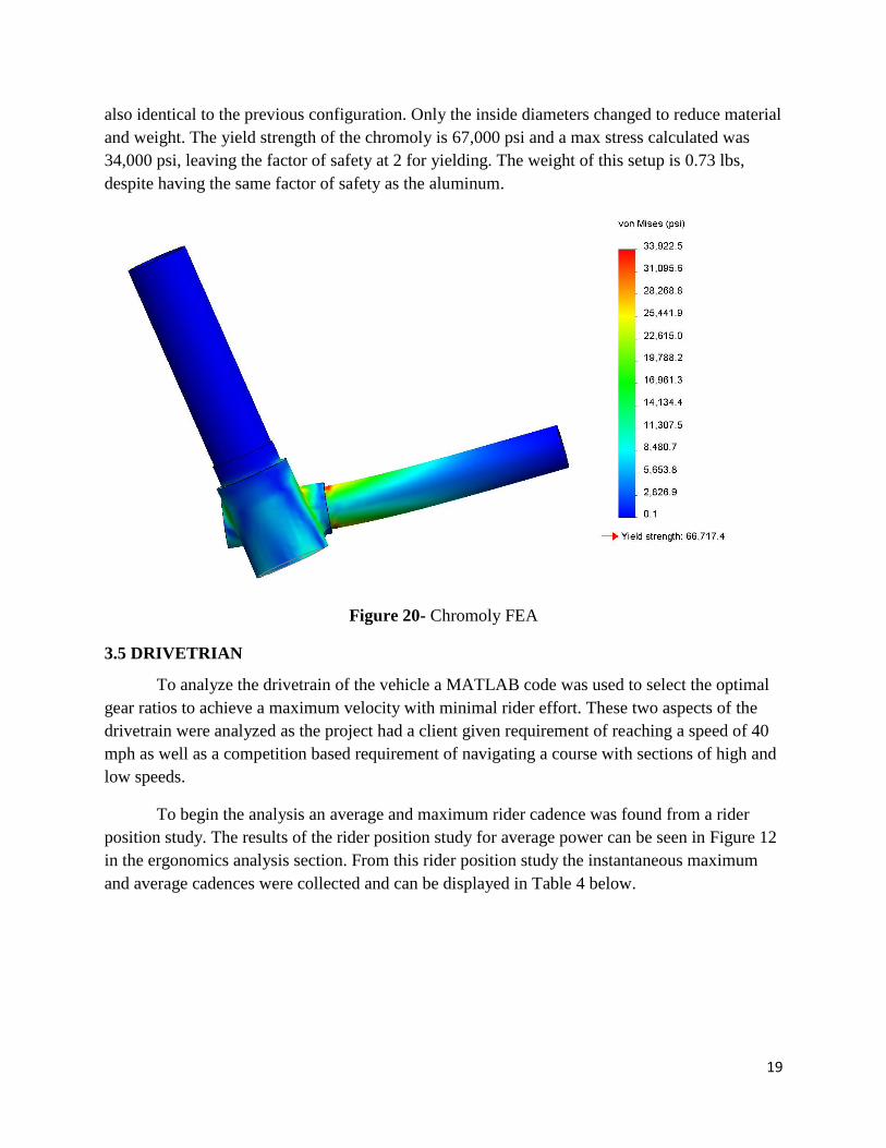
The next configuration is 4130 chromoly, seen in Figure 20. This configuration was
optimized to make the tubes as thin as possible while minimizing stresses. The force and fixtures
applied were the same as the previous configuration. The outside dimensions of this setup are
Page 20
19
also identical to the previous configuration. Only the inside diameters changed to reduce material
and weight. The yield strength of the chromoly is 67,000 psi and a max stress calculated was
34,000 psi, leaving the factor of safety at 2 for yielding. The weight of this setup is 0.73 lbs,
despite having the same factor of safety as the aluminum.
Figure 20- Chromoly FEA
3.5 DRIVETRIAN
To analyze the drivetrain of the vehicle a MATLAB code was used to select the optimal
gear ratios to achieve a maximum velocity with minimal rider effort. These two aspects of the
drivetrain were analyzed as the project had a client given requirement of reaching a speed of 40
mph as well as a competition based requirement of navigating a course with sections of high and
low speeds.
To begin the analysis an average and maximum rider cadence was found from a rider
position study. The results of the rider position study for average power can be seen in Figure 12
in the ergonomics analysis section. From this rider position study the instantaneous maximum
and average cadences were collected and can be displayed in Table 4 below.
Page 21
20
Table 4- Rider Cadence
Average Cadence (RPM) Max Cadence (RPM)
Rider 1 70 149
Rider 2 101 133
Rider 3 91 149
Rider 4 93 141
Rider 5 91 135
Rider 6 90 143
Average 89.33 141.67
Rounded Average 90 140
The results presented in the table allowed the team to select two cadence values to be
used in analysis. These included an average cadence of 90 rpm for extended periods of time and
a maximum cadence of 110 rpm when a top speed is desired. The value of 110 rpm was selected
by viewing the maximum instantaneous cadences displayed in the table, 140 rpm, and selecting a
cadence that was 20% lower than the lowest achieved maximum in order to better represent an
achievable maximum.
After establishing the two rider cadences to be analyzed, the team used a MATLAB code
to calculate the gear ratios and respective speeds for the vehicle. In order to achieve the client
requirement of reaching 40 mph the team chose to select a gear ratio that provided a max speed
5% over the requirement, a maximum speed of 42.25 mph. The vehicle needed to reach this
speed while attaining the lowest gear ratio on the easiest gears. Table 5 below displays the gear
ratio and speed at each of the positions on the rear cassette.
Table 5– Gear Ratios and Speeds
Gear
Ratio
Speed at 90
RPM (MPH)
Speed at 110
RPM (MPH)
1.50 10.56 12.91
1.69 11.88 14.52
1.93 13.58 16.60
2.25 15.84 19.36
2.57 18.11 22.13
3.00 21.13 25.82
3.38 23.77 29.05
3.86 27.16 33.20
4.50 31.69 38.73
4.91 34.57 42.25
Page 22
21
As seen in the table, the vehicle has a gear ratio of reaching 42.25 mph while having a
gear ratio of 1.5 in the lowest possible gear. By selecting a configuration with a low gear ratio
the vehicle will be capable of the start and stop motion on the course as well as reaching a max
speed.
3.6 INNOVATION
The team intends to design a vehicle that is operable in a range of climate conditions. Of
upmost concern was comfort of the rider in warm conditions. Even mildly warm ambient air
temperatures can make the interior vehicle a harsh environment for physical activity. With this in
mind, the team is designing a method for circulating ambient air through the shell during
operation in typical weather. This system will be passive, lightweight, and removable to
condition the incoming air in more adverse environments.
The first design placed a cold, finned block in line with incoming circulation air, with the
intention that it would remove energy, thus cooling the air before it flows over the operator. The
block itself would be machined out of aluminum, with a sealed hollow cavity filled with water.
An ice core would allow the block to remain cold for longer periods of time. As the ice
undergoes phase transition to water, the fin base temperature will remain semi constant. The
large amount of energy required to force the phase transition, as represented by the Heat of
Fusion, will allow for more energy absorption. A vehicle owner would place the finned block in
their freezer for an adequate amount of time prior to driving the vehicle, at which time, the block
would be mounted in its location inside the vehicle shell. As warm air passes over the fins, its
energy is transferred to the aluminum fins and ice core, eventually melting the internal ice and
raising it to ambient temperature. A concept model of this system can be seen in Figure 21, with
the blue mass representing the cold block.
Figure 21– Innovation
Page 23
22
With internal vehicle dimensions unavailable, a generous model was developed to
represent a plausible outcome for finned surface area with favorable material properties. An
assumption of 6 fins with .1m by .05 m dimensions was made, with their thickness small enough
to be negligible. The thermal resistance of the aluminum block shell was also assumed
negligible, effectively modeling the fins and base as made from ice itself. A convection
coefficient, h, was calculated using from Equation 10 for mixed boundary layer conditions.
(10)
where
(
)
(11)
And
(12)
Equations 10, 11, and 12 result in a convection coefficient of 31
at a velocity off 9
m/s (20 mph). Assuming an ambient air temperature, a surface area, and a flow rate of 26°C,
.0625 m2, and 9 m/s respectively, the ice will remain within 12° of its initial temperature for
roughly 46 minutes. 46 minutes is a sufficient period of time for a cooling system to operate,
however this design is limited by quality of performance rather than longevity of performance.
The system is limited by its small size and weight constraints which simply do not allow for
amount of surface area required to produce the desired cooling of incoming air. With the current
assumptions, only a 1°C temperature drop is achieved.
The team plans to explore methods to increase the surface area exposed to incoming
airflow as well as evaluate the efficacy of a small scale evaporative cooling mechanism that
would replace the finned cold block concept.
The air for system will enter the vehicle interior through a servo operated, closable duct
embedded into the composite fairing. This duct is operated by the vehicle rider through the use
of a button in the cockpit. The ability to close the duct serves two purposes. First, as daytime
high temperatures drop, the rider may find that they wish for a warmer environment to travel in.
Closing the duct will reduce air circulation and begin to increase the interior temperature as the
rider’s body puts out heat. Secondly, these ducts will introduce a measureable amount of
aerodynamic drag on the vehicle; the ability to seal off this port will give the rider the option to
temporarily sacrifice internal temperature for a higher vehicle velocity.
Page 24
23
As previously stated, this duct will be actuated by a servo with 180° of operating range.
The linkage that transfers rotation from the servo to the duct flap is designed so that lockout
occurs at the extremes of the flap position, requiring a minimal amount of batter power to hold
the flap in any one location. This is achieved with the usage of an 8:1 lever arm ratio. This part
will be fabricated using a fused deposition modeling additive manufacturing process.
Lighting systems are the competition standard for roadway communication. Brake lights,
tail lights, headlights, and turn signals are required for maximum competition ranking. However,
the quality and visibility of such lights is not regulated.
After evaluating the visibility of lights of automobiles the team found it necessary for any
light on a vehicle to be visible from a minimum of 180° horizontally. This requirement is
flexible in that it allows either the hardware of the light itself to be visible or a clear,
unquestionable view of the light emitted by the hardware.
It was also determined that successful turn signals must be visible from behind, to the
side, and in front of the vehicle. Rather than placing two turn signal light sets on the human
powered vehicle like those of an automobile, the team will include a continuous LED strip
around the circumference of the front wheel fairings. The arrangement of the light safety and
communication systems and their ranges of visibility can be seen in Figure 22.
Figure 22- Vehicle Lighting Arrangement
The team wanted to ensure that the vehicle would resist roll over during aggressive
driving. To accomplish this, the width of the vehicle was designed so that the tires would lose
traction before the vehicle initiated a tip.
Analysis was performed to determine the minimum front wheel width that would avoid
tipping conditions. First a total vehicle and rider weight of 240lbs was assumed to be distributed
evenly over all three wheels during static scenarios. However, for tipping conditions to occur, all
Page 25
24
the system’s mass would be carried by the rear and one front wheel. This creates a new
distribution of 80lbs per tire in contact with the ground. The static friction coefficient, , of
rubber on asphalt was assumed to be 0.8. The total system center of gravity was assumed at the
mid plane of the vehicle, 50% of the way between the front and back wheels, and 14in above the
ground.
For tipping to occur during an aggressive turn, the lateral inertial force, , acting at the
center of gravity must be so great that the moment it creates about the tire contact patches must
be greater than the moment created by the vehicle weight about the same contact patch.
However, the lateral inertial force must also be lower in magnitude than the maximum
frictional force, , before movement begins, where
(13)
Or in this case
(14)
Finally, slipping at both wheels in contact with the ground is not required to avoid a tip.
One wheel breaking loose will cause a shift in the vehicle’s direction of travel and weight
distribution to adequately avoid a tip.
If slipping is to occur before tipping, the lateral inertial force F required to overcome the
weight of the vehicle must be significantly greater than the maximum frictional force at either
of the two tires carrying the load of the vehicle. See Figure 23 for a diagram of the force
relationship.
Figure 23- Tipping Analysis FBD
F
W
N
𝒇
Page 26
25
For a three wheeled vehicle, lateral tipping occurs about an axis drawn from the contact
patch of either of the two front wheels to the contact patch of the rear wheel, also shown in
Figure 24. Because of this, the distance A from the center of gravity to the tipping axis is not
simply half the vehicle width. Instead, the distance to the tipping axis can be defined by the
geometry in Figure 24.
Figure 24- Tipping Axis Location
Solving for the minimum required distance A to avoid tipping requires setting and
can be seen below:
(15)
Substituting in the assumptions and solving for A gives
(16)
Back solving for the minimum front wheel width R gives
Page 27
26
(17)
(18)
23in was determined to be the minimum critical width to avoid tipping during aggressive
turning. However, bicycle lanes are usually a minimum of 48inches in width. Subsequently, the
width of the vehicle front wheels was chosen to be 42in, which will allow for a stable vehicle on
all types of terrain, yet still capable of traveling within bicycle specific lanes with space on either
side.
ASME continually pushes entrants to be innovative in the design and manufacturing of
their vehicles. Human powered vehicles are often one-off mobiles fabricated from exotic, costly
materials, especially when their main purpose is to be used as a competition entry. It was felt
that an effective way to offset these costs yet still have a vehicle that performs competitively was
to seek out alternative, recycled materials. More specifically, we will attempt to recycle scrap
materials from our own manufacturing of the vehicle. Tables 6 and 7 show a list of waste
materials traditionally produced during the fabrication of a human powered vehicle.
Combinations of these materials will be attempted, with the desire of creating a composite
material with properties that can be utilized on the vehicle. Currently the team is continuing to
collect these materials.
Table 6- Possible Recyclable Reinforcement Materials
Reinforcement Materials Source
Aluminum chips as collected or powered Machining of components
Wood Fibers Fixtures and shipping
Powdered previously laid up carbon fiber Last year’s vehicle, research projects
Cardboard Shipping supplies
Scrap carbon fiber and fiberglass clippings Local composite product manufactures
Table 7- Possible Recyclable Matrix Materials
Matrix Materials Source
Epoxy Resin Left over from previous and current builds
High density polyethlyne Discarded water bottles and shipping materials
Nylon Dupont material samples
Derlin Dupont material samples
ABS Contaminated FDM materials
Page 28
27
4.0 PROJECT SCHEDULE
The team is currently on schedule to complete the design and analysis portion of the
project by the 2013 winter break. In addition to the design and analysis phase, the team is also
ahead of schedule on the process of prototyping and ordering needed materials. The team will
work to stay on track based on the Gantt chart through the competition in May 2014. The Gantt
chart can be found in Appendix B, and displays the current progress on each task listed.
5.0 CONCLUSION
Team 9 has completed a series of analysis tasks in order to determine the best results for
each subsection of the vehicle. Each analysis task assisted in material selection, component
design, and vehicle configuration. Through the use of these numerical and analytical results, the
team was able to design an optimized vehicle.
As the frame of the vehicle is one of the core components, it was broken into three
separate components. These included the center tube, the outriggers, and the rollover protection
system. Through the analysis, the center tube and out riggers were will be made out of 1.5”X1.5”
aluminum square tubing. This will allow minimal torsional and lateral deflection while keeping
weight to a minimum. After completing finite element analysis, the roll bar protection system
proved to meet the ASME challenge requirements. The team conducted a series of experiments
to determine the ideal rider position. This rider study proved that an ideal angle of 122° would
provide the best average power while providing adequate visibility. Using the 122° rider position
a fairing size was optimized for the lowest coefficient of drag. This resulted in a faring of
roughly 108” in length, width of 22” and a height of 37”, with a coefficient of drag of 0.025. To
analyze the vehicles steering, four dimensions were evaluated: caster, camber, kingpin, and axle
offset. These results were a 13° caster angle, 12° camber angle, 30° kingpin angle and 0.5 in
angle offset. In addition to the steering geometry, the steering knuckle was analyzed using finite
element analysis. This proved that the knuckles should be made from aluminum and will have a
factor of safety of 2. Using the data collected from the rider position study the vehicles drivetrain
was analyzed to determine the optimal gear ratio while reaching a max speed above 40 mph. To
meet the competitions innovation requirements the team investigated a finned cold block cooling
system, safety systems and sustainable manufacturing. To analyze vehicle safety a lighting
system was evaluated and a tipping analysis was computed to find the vehicles width of 42in.
Lastly, the use of recycled materials was investigated to find potential materials for future
testing. Through all of the analysis completed, the team is on their way to building a vehicle
capable of meeting all requirements and goals set forth by the client and competition.
Page 29
28
6.0 REFERENCES
[1] R.C. Hibbeler, Structural Analysis, New Jersey, Pearson Prentice Hall, 2012
[2] R. G. Budynas and J. K. Nisbett, Shigley’s Mechanical Engineering Design, New York,
McGraw-Hill, 2011
[3] Philip J. Pritchard and John C. Leylegian, Introduction to Fluid Mechanics, Manhattan
College: John Wiley & Sons, Inc., 2011.
[4] R. Horwitz. (2010). The Recumbent Trike Design Primer (8.0) [Online].
Available: http://hellbentcycles.com/trike_projects/Recumbent%20Trike%20Design%20Pri
mer.pdf
[5] R.C. Hibbeler, Engineering Mechanics – Statics, Pearson Prentice Hall, 2010
Page 30
29
7.0 APPENDIX
APPENDIX A– Accelerometer Data
- Test 1 is a run at low speed towards two .75inch tall wood slats - accelerometers on rear
axle the maximum applied force for test 1 is 222.5 LBS
- Test 2 is a run at high speed towards two .75inch tall wood slats - accelerometers on rear
axle the maximum applied force for test 2 is 243.8 LBS
- Test 3 is a run at high speed towards two .75inch tall wood slats - accelerometers on front
axle the maximum applied force for test 3 is 271.8 LBS
- Test 4 is a run at high speed towards two .75inch tall wood slats - accelerometers on mid
belly of bike the maximum applied force for test 4 is 182.6 LBS
Page 33
32
APPENDIX B– Gantt Chart
Page 34
33
APPENDIX C– Coefficient of Drag Results
Table 8- Change in Length
Length (in) Width (in) Height (in) Speed (in/s) Force (lbf) Area (in2) Cd
96 18 33 704 0.4572 595.12 0.033
102 18 33 704 0.3775 579.41 0.028
108 18 33 704 0.3897 576.73 0.029
96 18 37 704 0.5995 681.54 0.038
102 18 37 704 0.4110 670.37 0.026
108 18 37 704 0.5400 670.51 0.035
96 18 39 704 0.6008 727.01 0.036
102 18 39 704 0.4123 751.53 0.024
108 18 39 704 0.5919 718.78 0.036
96 20 33 704 0.3215 624.85 0.022
102 20 33 704 0.3020 611.54 0.021
108 20 33 704 0.3198 600.8 0.023
96 20 37 704 0.5132 716.58 0.031
102 20 37 704 0.4957 702.1 0.030
108 20 37 704 0.4895 701.49 0.030
96 20 39 704 0.5913 763.3 0.033
102 20 39 704 0.5336 755.25 0.030
108 20 39 704 0.5085 750.21 0.029
96 22 33 704 0.3878 662.26 0.025
102 22 33 704 0.4633 651.16 0.031
108 22 33 704 0.3926 633.91 0.027
96 22 37 704 0.5417 760.07 0.031
102 22 37 704 0.5659 753.55 0.032
108 22 37 704 0.4376 740.06 0.025
96 22 39 704 0.6102 809.7 0.032
102 22 39 704 0.5902 805.48 0.032
108 22 39 704 0.4914 792.63 0.027
96 24 33 704 0.4520 700.15 0.028
102 24 33 704 0.3914 683.3 0.025
108 24 33 704 0.3361 678.4 0.021
96 24 37 704 0.6170 803.72 0.033
102 24 37 704 0.5126 790.64 0.028
108 24 37 704 0.5767 788.48 0.032
96 24 39 704 0.7177 855.92 0.036
102 24 39 704 0.5843 844.81 0.030
108 24 39 704 0.5251 845.19 0.027
Page 35
34
Table 9- Change in Width
Length (in) Width (in) Height (in) Speed (in/s) Force (lbf) Area (in2) Cd
96 18 33 704 0.4572 595.12 0.033
96 20 33 704 0.3215 624.85 0.022
96 22 33 704 0.3878 662.26 0.025
96 24 33 704 0.4520 700.15 0.028
96 18 37 704 0.5995 681.54 0.038
96 20 37 704 0.5132 716.58 0.031
96 22 37 704 0.5417 760.07 0.031
96 24 37 704 0.6170 803.72 0.033
96 18 39 704 0.6008 727.01 0.036
96 20 39 704 0.5913 763.3 0.033
96 22 39 704 0.6102 809.7 0.032
96 24 39 704 0.7177 855.92 0.036
102 18 33 704 0.3775 579.41 0.028
102 20 33 704 0.3020 611.54 0.021
102 22 33 704 0.4633 651.16 0.031
102 24 33 704 0.3914 683.3 0.025
102 18 37 704 0.4110 670.37 0.026
102 20 37 704 0.4957 702.1 0.030
102 22 37 704 0.5659 753.55 0.032
102 24 37 704 0.5126 790.64 0.028
102 18 39 704 0.4123 751.53 0.024
102 20 39 704 0.5336 755.25 0.030
102 22 39 704 0.5902 805.48 0.032
102 24 39 704 0.5843 844.81 0.030
108 18 33 704 0.3897 576.73 0.029
108 20 33 704 0.3198 600.8 0.023
108 22 33 704 0.3926 633.91 0.027
108 24 33 704 0.3361 678.4 0.021
108 18 37 704 0.5400 670.51 0.035
108 20 37 704 0.4895 701.49 0.030
108 22 37 704 0.4376 740.06 0.025
108 24 37 704 0.5767 788.48 0.032
108 18 39 704 0.5919 718.78 0.036
108 20 39 704 0.5085 750.21 0.029
108 22 39 704 0.4914 792.63 0.027
108 24 39 704 0.5251 845.19 0.027
Page 36
35
Table 10- Change in Height
Length (in) Width (in) Height (in) Speed (in/s) Force (lbf) Area (in2) Cd
96 18 33 704 0.4572 595.12 0.033
96 18 37 704 0.5995 681.54 0.038
96 18 39 704 0.6008 727.01 0.036
96 20 33 704 0.3215 624.85 0.022
96 20 37 704 0.5132 716.58 0.031
96 20 39 704 0.5913 763.3 0.033
96 22 33 704 0.3878 662.26 0.025
96 22 37 704 0.5417 760.07 0.031
96 22 39 704 0.6102 809.7 0.032
96 24 33 704 0.4520 700.15 0.028
96 24 37 704 0.6170 803.72 0.033
96 24 39 704 0.7177 855.92 0.036
102 18 33 704 0.3775 579.41 0.028
102 18 37 704 0.4110 670.37 0.026
102 18 39 704 0.4123 751.53 0.024
102 20 33 704 0.3020 611.54 0.021
102 20 37 704 0.4957 702.1 0.030
102 20 39 704 0.5336 755.25 0.030
102 22 33 704 0.4633 651.16 0.031
102 22 37 704 0.5659 753.55 0.032
102 22 39 704 0.5902 805.48 0.032
102 24 33 704 0.3914 683.3 0.025
102 24 37 704 0.5126 790.64 0.028
102 24 39 704 0.5843 844.81 0.030
108 18 33 704 0.3897 576.73 0.029
108 18 37 704 0.5400 670.51 0.035
108 18 39 704 0.5919 718.78 0.036
108 20 33 704 0.3198 600.8 0.023
108 20 37 704 0.4895 701.49 0.030
108 20 39 704 0.5085 750.21 0.029
108 22 33 704 0.3926 633.91 0.027
108 22 37 704 0.4376 740.06 0.025
108 22 39 704 0.4914 792.63 0.027
108 24 33 704 0.3361 678.4 0.021
108 24 37 704 0.5767 788.48 0.032
108 24 39 704 0.5251 845.19 0.027
Page 37
36
APPENDIX D– Rider Position Study Data