Huo Peng

ROAD TRAFFIC MONITORING USING

NOISE SENSOR NETWORKS:

VEHICLE SPEED DETECTION

Technology and Communication

2011

VAASAN AMMATTIKORKEAKOULU

UNIVERSITY OF APPLIED SCIENCES

Degree Programme

ABSTRACT

Author Huo Peng

Title Road Traffic Monitoring Using Noise Sensor Networks:

Vehicle Speed Detection

Year 2011

Language English

Pages 44

Name of Supervisor Gao Chao

Using noise sensor networks is one of the applications to monitor road traffic.

Normally the equipments which are used to measure are much expensive. The

purpose of this project was to use the low-cost wireless sensor networks to moni-

tor the vehicle‟s speed and calibrate the accuracy of the result.

Actually we set two wireless sensors which are separated by a specific distance

beside the highway and we collect the data of the vehicle passing this road during

the specific time. Then we calculate the time difference of the vehicle passing

these two sensors. At the end using distance divides time difference we can know

the vehicle‟s speed.

From the calibration we can know the result is accurate but there is a little bit er-

ror. So the algorithm can still be improved to provide a more accurate result in the

future.

Keywords wireless sensor, road traffic monitoring

3

ABBREVIATIONS

ADC Analog-to-Digital Converter

IEC International Electrotechnical Commission

MATLAB MATRIX LABORATORY

RMS Root Mean Square

SPL Sound Pressure Level

4

CONTENTS

ABSTRACT

1 INTRODUCTION ................................................................................................ 5

2 BACKGROUND .................................................................................................. 6

2.1 Sound Level .................................................................................................. 6

2.2 Brief measurement procedure ...................................................................... 7

2.3 The requirement of the measurement system ............................................ 8

2.4 Synchronization .......................................................................................... 10

2.5 The Standard Calibrator Comparison ........................................................ 12

3 MEASUREMENT EXPERIMENTS ................................................................ 15

4 ALGORITHM OF SPEED DETECTION ........................................................ 16

4.1 Data in the files ........................................................................................... 17

4.2 MATLAB extract data from the text file .................................................. 18

4.3 Extract data of the two nodes and save it into two vectors ...................... 19

4.4 Checking missing data ............................................................................... 20

4.5 Linear Interpolation .................................................................................... 21

4.6 Filter the data .............................................................................................. 26

4.7 Two ways of finding the time difference .................................................. 28

4.8 Choosing the way to calculate the time difference ................................... 29

4.9 How to use the slope to find speed ............................................................ 30

4.10 How to find the right parameters ............................................................... 31

4.10.1 Find peaks ....................................................................................... 34

4.10.2 Find the right slope......................................................................... 37

4.10.3 Find the right intercept ................................................................... 37

4.10.4 Calculate the time difference ......................................................... 38

4.11 The calculation result on the graph ........................................................... 39

4.12 Calibration ................................................................................................... 40

4.12.1 Introduce the calibration procedure .............................................. 40

4.12.2 Calibration ...................................................................................... 40

5 CONCLUSION .................................................................................................. 42

REFERENCES .......................................................................................................... 44

5

1 INTRODUCTION

Road traffic monitoring includes many factors and monitoring vehicle speed is

our application. Nowadays there are lots of methods to measure. In this project,

we apply an environment noise sensor network to monitor the vehicle speed.

Actually we set two noise wireless sensors beside the highway to collect the data

of the environment noise. Then we set one sink which connected to a laptop to

receive the packets send by sensors. When a vehicle passes the sensor, the data

collected by the sensor will have a big change. The change notifies that the vehi-

cle is passing the sensor. From the collected data we can calculate the time differ-

ence of one vehicle passing those two sensors and the initial the distance of the

two sensors is 40 meters. So the speed of the vehicle equals the 40 meters divide

the time difference of the vehicle passing the two sensors.

Normally we can buy the commercial sound meter on the market to measure, but

our application‟s devices are developed by Kokkola University Consortium. [1]

The general reason for using this system is that these devices are much cheaper

than the commercial sound level meters and this type of the system is synchroni-

zation. Only by the nodes of synchronization can we calculate the correct time

difference of the vehicle passing the two nodes. I will explain it more clearly in

Section 2.4.

The rest of this document is organized as follows: brief measurement procedure,

the requirement of the measurement system, sound level introduction, system con-

figuration, synchronization and the data format obtained from the sensors are

given in Chapter 2. The measurement experiments are described in Chapter 3. The

algorithm for processing the collected data and calculating the speed is depicted in

Chapter 4, as well as the calibration and the result. The conclusion is given in the

last Chapter.

6

2 BACKGROUND

2.1 Sound Level

Sound is a traveling wave, which is an oscillation of pressure transmitted through

a solid , liquid, or gas, composed of frequencies within the range of hearing and of

a level sufficiently strong to be heard. The sensation of sound is then produced by

the stimulation of hearing organs by such vibrations [2]. The human ear is a very

sensitive device and can hear sound power range of 12 to 13 decimal magnitudes

[3]. Sound power level is defined as a logarithm scale and denoted as decibels. It

can be calculated by

(1)

Where are root mean square sound pressure and reference sound

pressure,respectively, and (RMS).[4]

The frequencies can be heard by the human ear are from 20 Hz to 20 kHz. But the

human ear does not have a flat spectral response. Sound pressures are often fre-

quency weighted. The International Electrotechnical Commission (IEC) has de-

fined several weighting schemes. A-weighting attempts to match the response of

the human ear to noise. The corresponding transfer function of the A-weighting

filter is given, according to [5], as

(2)

means the sound level is measured after the A-weighting filter. The effective

sound pressure is the RMS value of the instantaneous sound pressure divides a

given interval time. means the equivalent sound level over time T. In our

system the T = 125 ms and the equation is that:

7

In the equation N is the number of samples taken at time T. In our design, a set of

digital and analog amplifications is controlled to produce a suitable ADC range.

All these amplifications together with can be considered as a single constant

value that can be retrieved by comparing the ADC reading with a standard

calibrator [1].

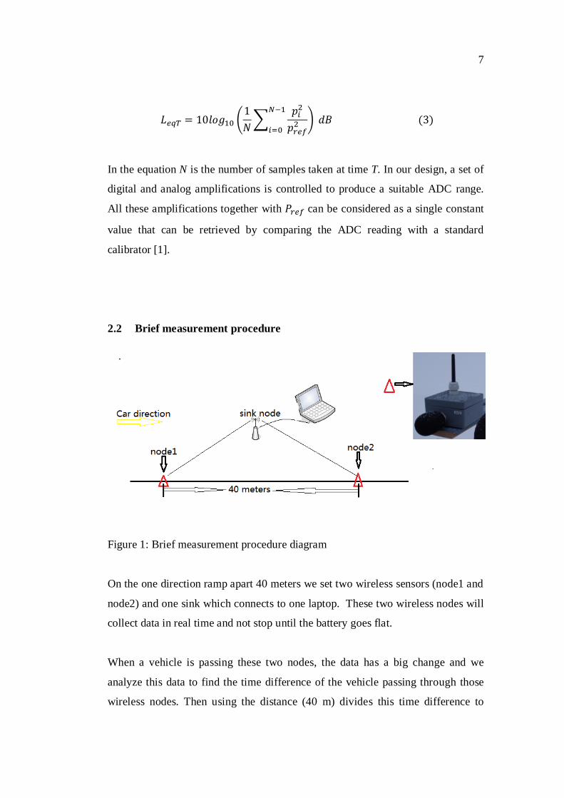
2.2 Brief measurement procedure

Figure 1: Brief measurement procedure diagram

On the one direction ramp apart 40 meters we set two wireless sensors (node1 and

node2) and one sink which connects to one laptop. These two wireless nodes will

collect data in real time and not stop until the battery goes flat.

When a vehicle is passing these two nodes, the data has a big change and we

analyze this data to find the time difference of the vehicle passing through those

wireless nodes. Then using the distance (40 m) divides this time difference to

8

calculate the vehicle speed. Actually how to find the time difference which will

be illustrated in Section 4.7 and 4.8.

2.3 The requirement of the measurement system

1) Low-cost device and workload

2) Real-time result

3) Multi-point measurement

4) Coherent measurement

5) Minimal attention requirement

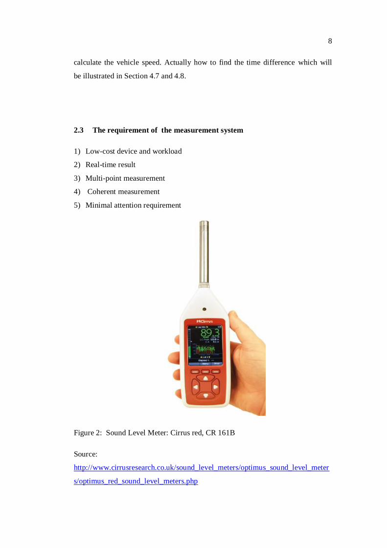
Figure 2: Sound Level Meter: Cirrus red, CR 161B

Source:

http://www.cirrusresearch.co.uk/sound_level_meters/optimus_sound_level_meter

s/optimus_red_sound_level_meters.php

9

Figure 2 shows the sound level meter which is the commercial sound level meter

and we use this SOUND LEVEL METER to calibrate.

The advantage of a commercial sound level meter is that the measurement sound

level result is more accurate than that of a low-cost sensor node. Therefore we use

this sound level meter to calibrate.

The disadvantages of the commercial sound level meter compare to our designed

system:

1) The commercial sound meters are expensive and making large-scale

measurements very costly.

2) Two sound level meters can not be synchronous.

3) The sound level meter can not supply real-time result.

4) The sound level meter has to be fully attended which increases the workload.

Figure 3: Our designed node

The advantage:

1) Cost reduction in equipment and workload.

2) Real-time, multi-point, coherent measurement

3) Minimal attention required.

10

The disadvantage I will illustrate in Section 2.5 and this disadvantage does not

affect our measurement so we choose this system to measure.

2.4 Synchronization

Figure 4: Synchronization diagram

Generally the whole system working procedure is that the two nodes collect data

and then send to the sink. The sink connects to a laptop and the data can be saved

as a (.csv) file on the laptop.

The concrete procedure shows in Figure 4:

The system works periodically and each period consists of three phases: broad-

casting, noise sampling, and data communication, respectively and the period is 5

seconds.

In the first phase the sink broadcasts a SYNC frame, which includes a

monotonically increasing sequence number from 0 to 255 periodically and the

current time of the sink. After the node receiving a copy of it, the node re-

broadcasts the SYNC frame to the rest of network. Base on the first phase a

11

passive route has been established for every node in the network. Generally the

time using in the first phase is less than 20 ms. Comparing to the other two

phases, this time is negligible

In the second phase, the node samples the noise data, the resolution is 125 ms (the

system is designed to be able to perform the fast measurement: the RMS power

calculation is done every 125 ms corresponding to A-weighting in IEC 61672. [1])

and the whole time is 4.5 seconds. So there are 36 RMS values.

In the third phase, the node sends a data frame back to sink which uses 0.5 second.

There are 4 zeros at the end because no measurement is done during the last

4*125 ms=0.5 second.

How the collected data looks like in the file I will show it in Section 4.1.

12

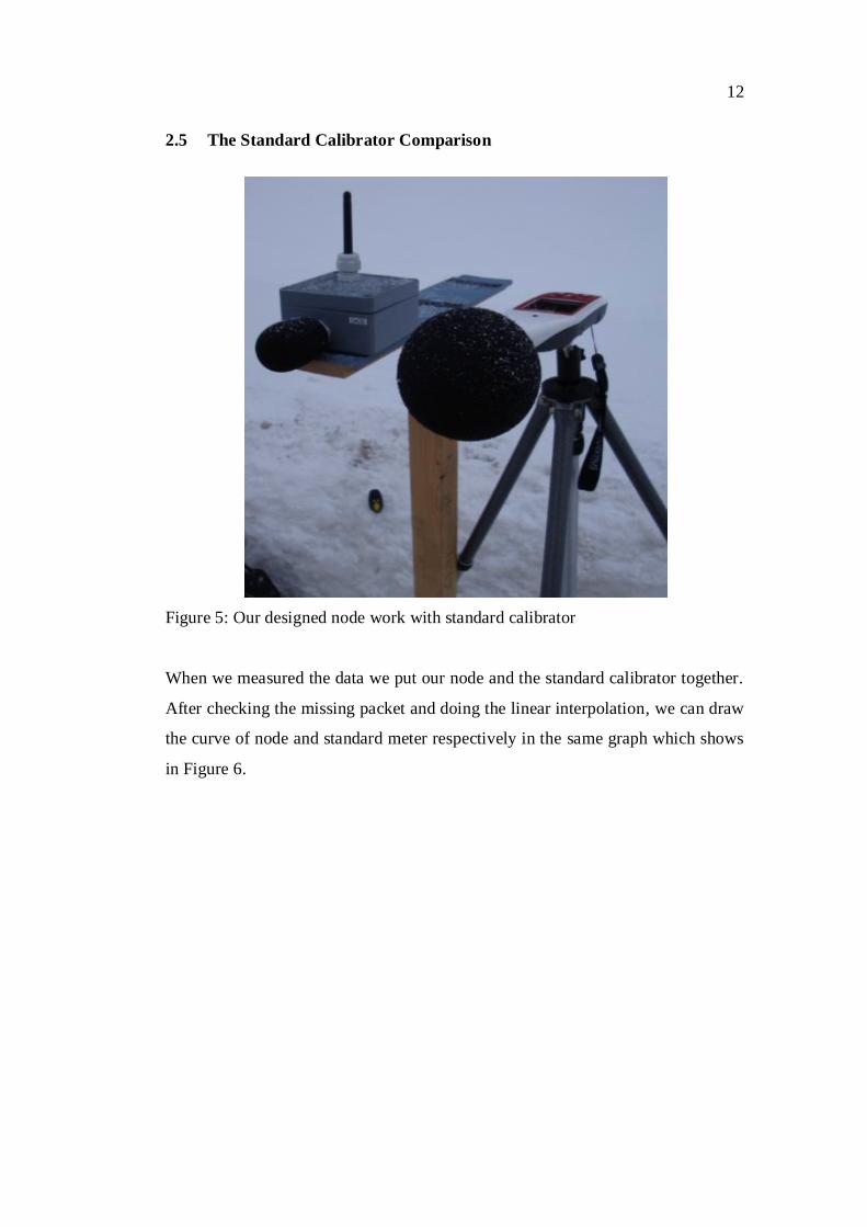
2.5 The Standard Calibrator Comparison

Figure 5: Our designed node work with standard calibrator

When we measured the data we put our node and the standard calibrator together.

After checking the missing packet and doing the linear interpolation, we can draw

the curve of node and standard meter respectively in the same graph which shows

in Figure 6.

13

Figure 6: Node vs. Calibrator (Blue=node, Magenta=calibrator)

From Figure 6 we can see exactly the node and the calibrator can collect the data

at the same time and the shapes of two curves are almost the same. A few differ-

ences show in Figure 7 below.

Figure 7: Enlarge the curves of the node and the meter

14

From Figure 7 we can see the scale range of the data from the node is wider than

it from the meter. But looking at the peaks, there are some ripples on the node

curve. To measure the vehicle speed we only need to know when the peak occurs

and the smoothly climbing up curve. The reason I will illustrate in Section 4.7.

The exact peak value it does not need in the vehicle speed calculation. So we can

conclude that the data from the node satisfies our requirements.

15

3 MEASUREMENT EXPERIMENTS

Figure 8: The location of the measurement

The location of E12 exit ramp to Airport Park Vaasa shows in Figure 8.

In our measurement we need find a one-way road to collect data, because if we

measure on a two-way road, the node will also collect the data from the opposite

road and our algorithm can not distinguish the vehicle belong to which side of the

road which will interfere us to find the correct time difference of one vehicle pass-

ing the two nodes.

The date is on 31.1.2011, the time is at 13:00 and the duration is 45 minutes.

The weather condition is snowy and the road condition is one way ramp.

16

4 ALGORITHM OF SPEED DETECTION

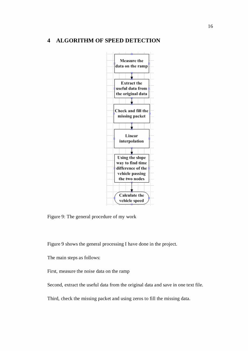
Figure 9: The general procedure of my work

Figure 9 shows the general processing I have done in the project.

The main steps as follows:

First, measure the noise data on the ramp

Second, extract the useful data from the original data and save in one text file.

Third, check the missing packet and using zeros to fill the missing data.

17

Fourth, using the slope way to find the time differences of the vehicles passing

through the two nodes.

Fifth, calculate the vehicle speed.

4.1 Data in the files

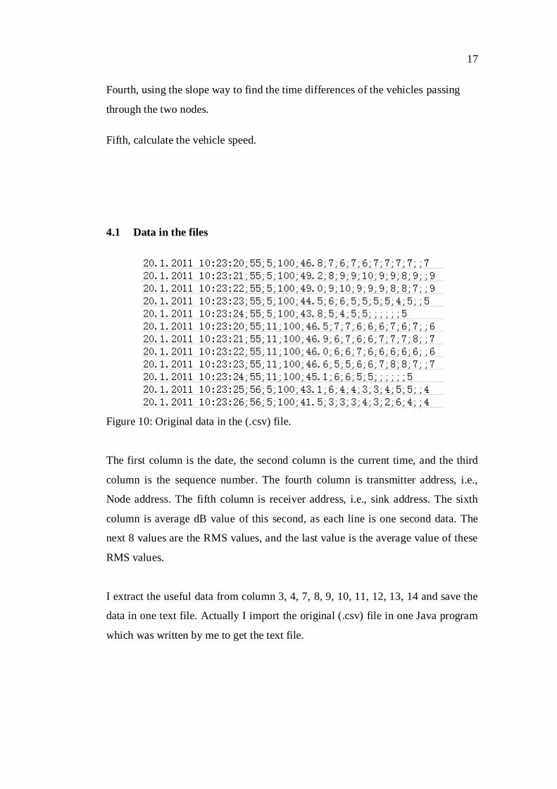
Figure 10: Original data in the (.csv) file.

The first column is the date, the second column is the current time, and the third

column is the sequence number. The fourth column is transmitter address, i.e.,

Node address. The fifth column is receiver address, i.e., sink address. The sixth

column is average dB value of this second, as each line is one second data. The

next 8 values are the RMS values, and the last value is the average value of these

RMS values.

I extract the useful data from column 3, 4, 7, 8, 9, 10, 11, 12, 13, 14 and save the

data in one text file. Actually I import the original (.csv) file in one Java program

which was written by me to get the text file.

18

Figure 11: The data in the text file.

Figure 11 shows the first column is the sequence number, the second column is

node number and the next eight values are the RMS which I need analysis.

4.2 MATLAB extract data from the text file

The MATLAB code:

[seqn src a1 a2 a3 a4 a5 a6 a7 a8]

= textread('four.txt','%d%d%d%f%d%d%d%d%d%d');

In the MATLAB code I use textread() function to extract the import data

from the text file. Exactly I define the column name of data ahead the equal opera-

tor, after the equal operator I declare the data type which is double. „four.txt‟ is

the txt file name. a1 to a8 are the vectors contain data which are extracted from

the file in columns.

19

4.3 Extract data of the two nodes and save it into two vectors

Use the unique() function to filter the src data which contains the node num-

ber. Because there are only two nodes, vector srcadd=[5 , 11]. “5” and “11”

are the node number which can be seen in Figure 11.

a1 to a8 are the vectors contain data which are extracted from the file in columns.

So they contain data both from two nodes.

“src1a1 = a1(find (src==srcadd(1)));” means find data from a1 of

node 5.

After this step I create a vector src1a which will contain all the data from node 5.

And then I use one for-loop put all the data from node 5 into this vector which

likes below:

For k=1:length(src1a1)

src1a=[src1a src1a1(k) src1a2(k) src1a3(k) src1a4(k)

src1a5(k) src1a6(k) src1a7(k) src1a8(k)];

end

db1a = 8.5192*log(src1a) + 30.59;

The logic shows below to prevent log (zero) problem.

src1a = src1a + (src1a==0);

Use the equation which shows below to convert RMS data into dB value.

(4)[1]

20

So the vector db1a contains all the dB values belong to node 5.

By the way I can get vector db2a which contains all the dB values belong to node

11.

4.4 Checking missing data

Figure 12: Checking missing data block diagram.

Generally at the first step defines two vectors and extracts the sequence number of

those two nodes and saves into these two vectors, respectively.

The second step uses MATLAB diff() function to process these two vectors.

How the diff() function works which explains in Figure 12.

The third step uses find() function to find the data missing location and saves

in vector misLoc. Because the sequence number should be continuous, the values

21

in the vector only have three conditions: 1, 0 and -255. In every 5 seconds the sink

receives the data so the same sequence number will appear 5 times and the num-

ber “0” will appear in the vector. After 5 seconds the sink will send an increasing

sequence number so the number “1” will appear in the vector. The sequence num-

ber periodically starts from 0 to 255 so in the current period the sink sends the last

sequence number is 255 and in the next period the sink sends the first sequence

number is 0 so that the number “-255” will appear in the vector.

The fourth step checks the values in the vector misLoc. If the vector misLoc is

empty which means there is no missing packet else the missing place is the value

in the vector misLoc.

The fifth step uses 40 zeros to fill all the places of the missing data.

After filling the missing data of the first node, I use the same way to solve the

other node.

4.5 Linear Interpolation

Why the data of the missing place must be done the linear interpolation? After

looking Figure 13 you will know the answer.

22

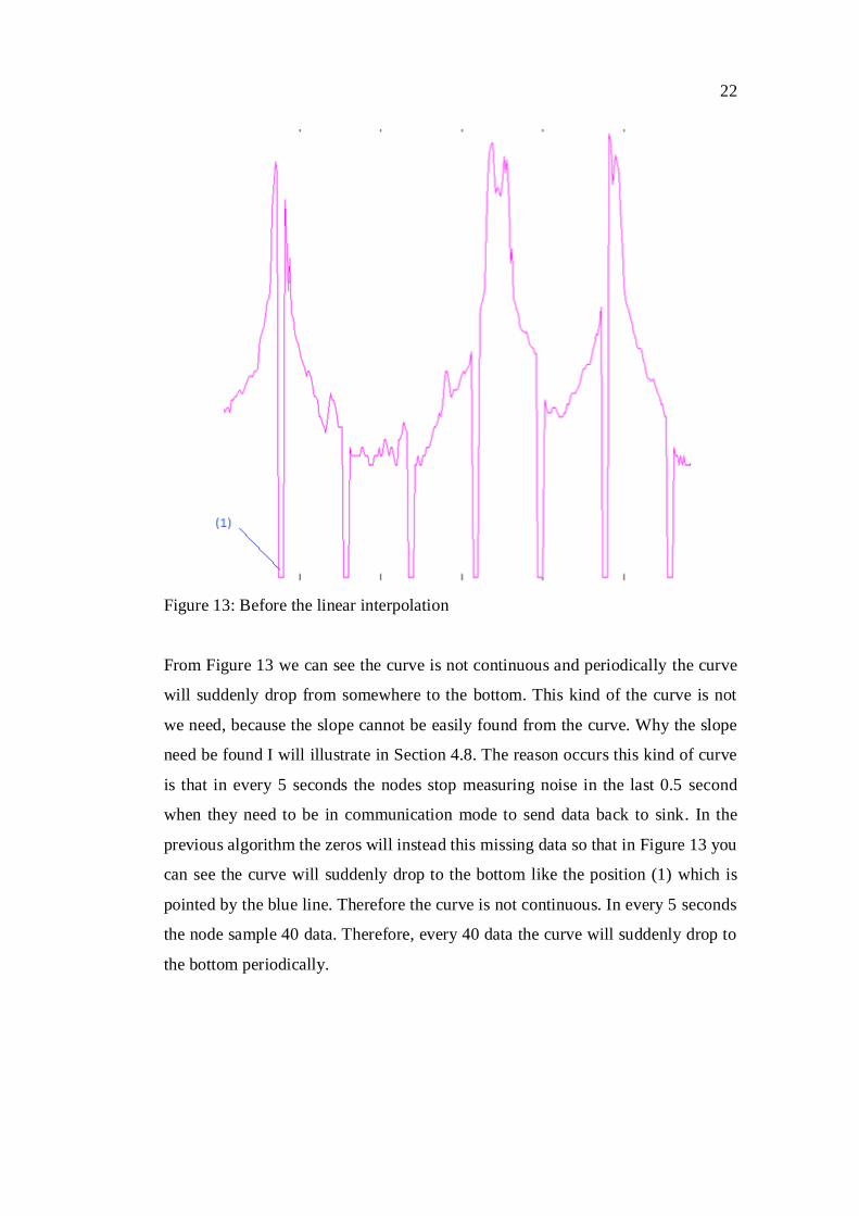
Figure 13: Before the linear interpolation

From Figure 13 we can see the curve is not continuous and periodically the curve

will suddenly drop from somewhere to the bottom. This kind of the curve is not

we need, because the slope cannot be easily found from the curve. Why the slope

need be found I will illustrate in Section 4.8. The reason occurs this kind of curve

is that in every 5 seconds the nodes stop measuring noise in the last 0.5 second

when they need to be in communication mode to send data back to sink. In the

previous algorithm the zeros will instead this missing data so that in Figure 13 you

can see the curve will suddenly drop to the bottom like the position (1) which is

pointed by the blue line. Therefore the curve is not continuous. In every 5 seconds

the node sample 40 data. Therefore, every 40 data the curve will suddenly drop to

the bottom periodically.

23

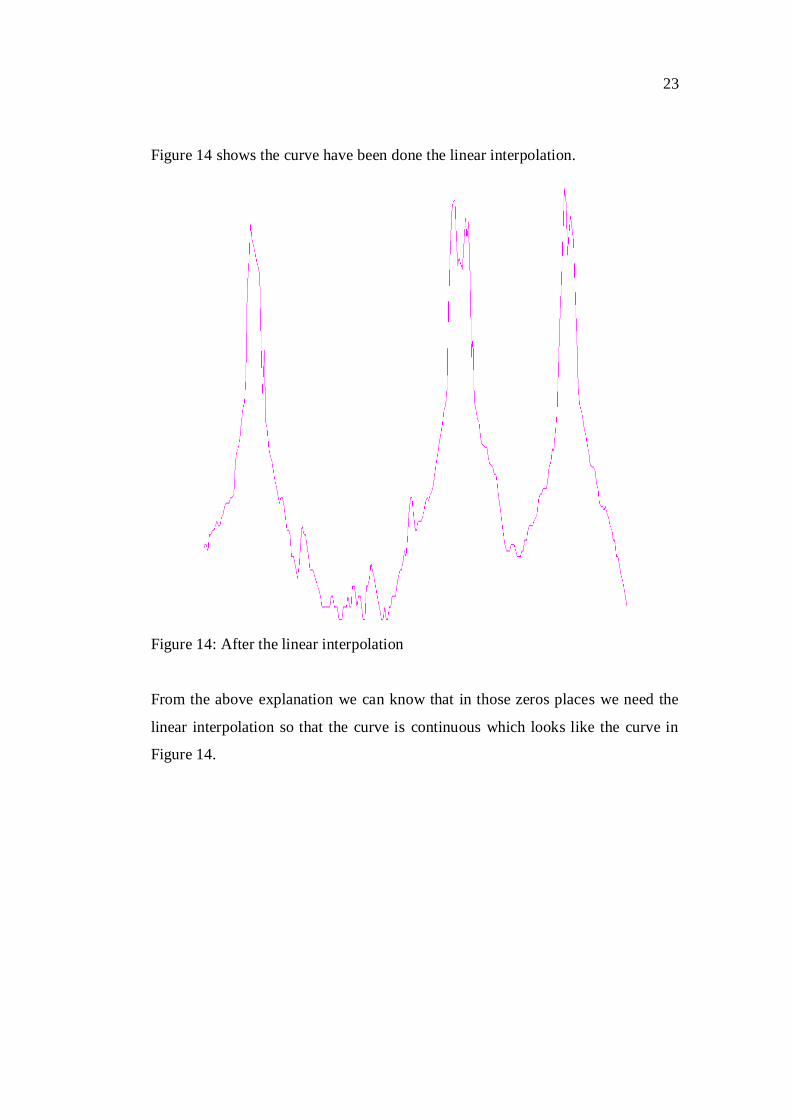
Figure 14 shows the curve have been done the linear interpolation.

Figure 14: After the linear interpolation

From the above explanation we can know that in those zeros places we need the

linear interpolation so that the curve is continuous which looks like the curve in

Figure 14.

24

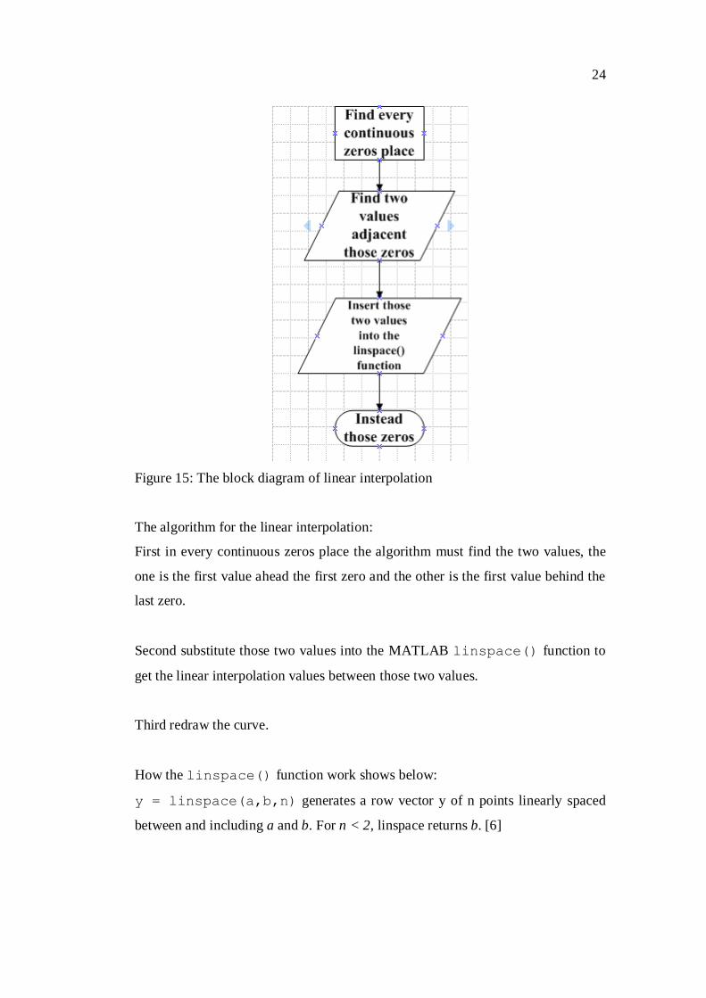
Figure 15: The block diagram of linear interpolation

The algorithm for the linear interpolation:

First in every continuous zeros place the algorithm must find the two values, the

one is the first value ahead the first zero and the other is the first value behind the

last zero.

Second substitute those two values into the MATLAB linspace() function to

get the linear interpolation values between those two values.

Third redraw the curve.

How the linspace() function work shows below:

y = linspace(a,b,n) generates a row vector y of n points linearly spaced

between and including a and b. For n < 2, linspace returns b. [6]

25

In every 5 seconds there are 4 zeros at the end of the collected data which means

of every 40 data there are 4 zeros at the end. So in every 40 data I use the

MATLAB linspace() function to do the linear interpolation and instead this

zeros.

In the end of all the data there are 4 zeros so the value behind the last zero cannot

be found, in this condition we substitute the first value ahead the first zero and the

zero into the linear interpolation function to find the linear interpolation values.

Except the last 40 data linear interpolation, I substitute two adjacent data of the 4

zeros into the linspace() function.

In the missing data place we use 40 zeros to fill. So in those zero places we also

need to do the linear interpolation. First find one value first ahead the first zero of

the 40 zeros and then find the other value first behind the last zero of the 40 zeros.

Second substitute those two values into the linear interpolation function.

After solving the first node I use the same way to solve the other node.

26

4.6 Filter the data

After checking the missing packet and doing the linear interpolation we can draw

two node‟s curves in the same graph which shows in Figure 16.

Figure 16: The original two node graphs

(Blue represents Node 1 (address 5); Magenta represents Node 2 (address 11))

We can easily see from Figure 16 there are lots of ripples in the peaks and even in

some places of the rising curve.

In order to find curve peaks correctly, we must use the filter function to remove

those ripples on the peaks. The reasons are that the ripples will impact to find real

peaks and the ripples in the rising curve will impact to find the peak ascending

side width which will be used in the slope calculation.

Figure 17 show below is the curve after being filtered. Exactly I use lowpass filter

to remove those ripples. In lowpass function we set the cutoff frequency which

27

equals 0.8 Hz and the order of FIR which equals 21. The sampling frequency

equals 8 Hz, because the node in one second will collect 8 samples.

Figure 17: The two node graphs after filtering,

In the code the fir1() function is used to make lowpass filter.

How the fir1() function work is shown below:

b = fir1(n,Wn) returns row vector b containing the n+1 coefficients of an

order n lowpass FIR filter.[7]

Wn equals the cutoff frequency divide the sampling frequency. The notice is that

“n” multiply “Wn” must be greater than 1.

28

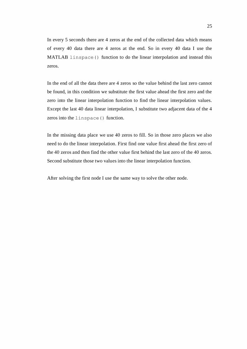
4.7 Two ways of finding the time difference

As we know the speed equals the distance divides the time and the distance is the

constant value (40 meters), so the main work is to find the time difference of the

vehicle passing the two nodes.

There are two ways to find the time difference of the vehicle passing the two

nodes which show in Figure 18.

Figure 18: The two ways of finding the time difference

The first way shows on the left of Figure 18 is that find the two peaks of the two

curves and then calculate the time difference of those two peaks.

The second way shows on the right of Figure 18 is that find the two slopes of the

curves and then calculate the time difference of those two slopes.

So which way is more accurate and is used I will tell you in Section 4.8.

29

4.8 Choosing the way to calculate the time difference

Figure 19: The sample is processed by two ways

Normally the time difference calculated by using the peak way is almost the same,

but in the situation which shows in Figure 19 there is an apparent difference.

On the left of Figure 19 shows the peak way to process the data and in the right of

Figure 19 shows the slope way to process the data.

From Figure 19 we can see in this sample the time difference calculated by using

the peak way is smaller than the time difference calculated by using the slope way.

According to the record the time difference calculated by using the slope way is

close to the real result.

So the slope way is chosen to calculate the time difference of the vehicle passing

the two nodes.

How to use slope way to calculate I will explain in Section 4.9.

30

4.9 How to use the slope to find speed

Figure 20: The slope way

The linear equation of slope in the first curve is and the linear equa-

tion of slope in the second curve is . Suppose the second node‟s

slope is a time-shifted version of the first one. So we can set .

Because

We can get

Distance d=40 meters, Speed

So

31

From the calculation above we can know in order to calculate the speed we need

know the right

How to find the right those parameters I will explain in Section 4.10.

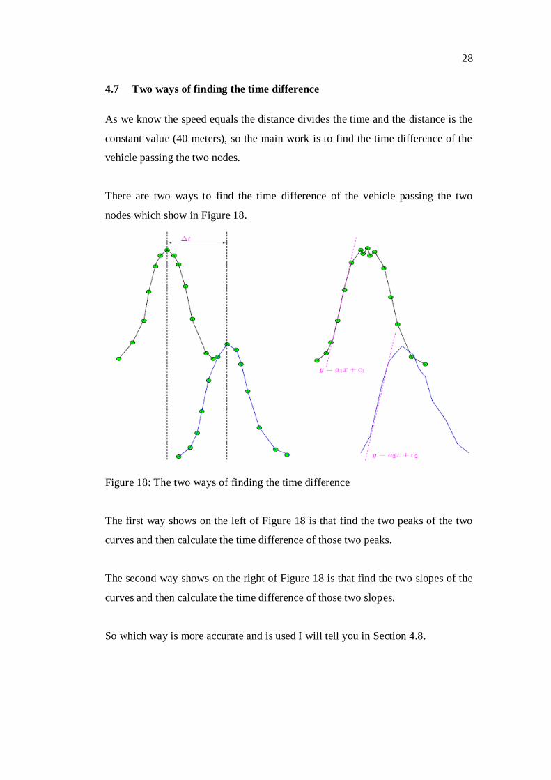
4.10 How to find the right parameters

Figure 21: The block diagram to find parameters

32

First find the two peaks ( ) of the two curves respectively.

Second in the first curve search ahead 3dB from to find the first point

( and search ahead 19dB to find second point ( ). Then use

these two points to draw a line . In the second curve use the same way to find

two points ( and and then use these two points to draw

a line .

Third find from these two lines and find a new parameter (a) which is

the average of and . Why use the average value I will explain in Section

4.10.2.

Fourth find the middle point ( of and in the first curve and then find

the middle point ( of and in the second curve.

Fifth use the new slope (a) and these two middle points and to create two

new lines and

. From these two lines to find and

.

All those parameters will show in Figure 22.

33

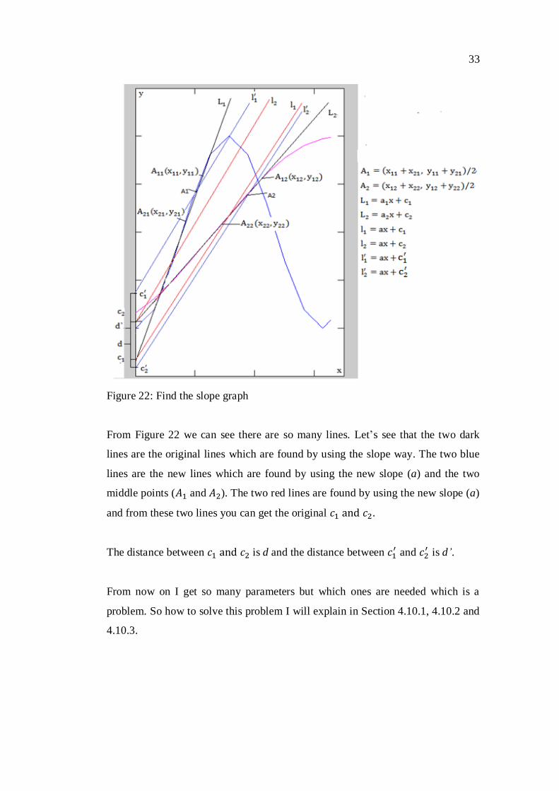
Figure 22: Find the slope graph

From Figure 22 we can see there are so many lines. Let‟s see that the two dark

lines are the original lines which are found by using the slope way. The two blue

lines are the new lines which are found by using the new slope (a) and the two

middle points ( and ). The two red lines are found by using the new slope (a)

and from these two lines you can get the original

The distance between is d and the distance between and

is d’.

From now on I get so many parameters but which ones are needed which is a

problem. So how to solve this problem I will explain in Section 4.10.1, 4.10.2 and

4.10.3.

34

4.10.1 Find peaks

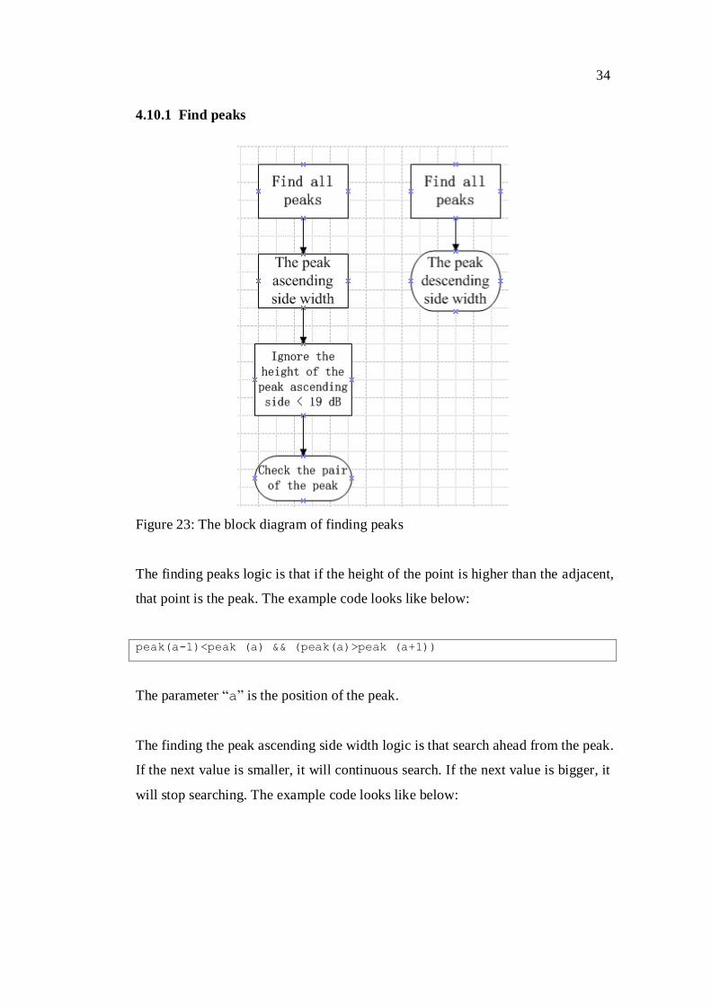
Figure 23: The block diagram of finding peaks

The finding peaks logic is that if the height of the point is higher than the adjacent,

that point is the peak. The example code looks like below:

peak(a-1)<peak (a) && (peak(a)>peak (a+1))

The parameter “a” is the position of the peak.

The finding the peak ascending side width logic is that search ahead from the peak.

If the next value is smaller, it will continuous search. If the next value is bigger, it

will stop searching. The example code looks like below:

35

while (peak(t)-peak(t-k)<=19 && peak(t-k-1)<=peak(t-k))

k = k+1;

end

fl=[fl k];

In the code above t is the position of the peak, so search ahead of this peak. The

parameter k is the counter to count the peak ascending side width. The vector fl

contains the peak ascending side width.

The finding the peak descending side width logic is that search behind from the

peak. If the next is smaller it will continuous search. If the next is bigger it will

stop searching. The example code looks like below:

while(peak(t)-peak(t+k)<=19 && peak(t+k+1)<=peak(t+k))

k=k+1;

end

fr=[fr k];

In the code above t is the position of the peak, so search behind from this peak.

The parameter k is the counter to count the peak descending side width. The vec-

tor fr contains the peak descending side width.

In the slope calculation we need find two points on the curve, one of the two

points is found by searching ahead 19 dB from peak. So we need to ignore the

height of the peak ascending side smaller than 19 dB.

36

The logic is that uses the height of peak value reduce the lowest height of the peak

ascending side width value. If the result is smaller than 19 dB I ignore this peak.

The code looks like below:

peak(k)-peak(k-fl(k))<19

After filtering the peaks we must check whether all the peaks are the pairs, be-

cause the speed calculation needs know the information from the two nodes at the

same time.

In the checking loop I add almost 3 seconds to the time of the vehicle passing the

first node and then use this time reduce the time of the vehicle passing the second

node. If the difference is smaller than 1.5 seconds I keep this peak. If not I will

delete this peak. The reason adding 3 seconds is that I suppose the lowest speed of

vehicle is 50 kilometers per hour. The code looks like below:

for k=1:length(peak1)

for t=1:length(peak2)

abs(peak2(t)-(peak1(k)+23))<12

newpeak1= [newpeak1 peak(k)];

end

end

The code above is to check the peak of the first node. It must use the same way to

check the peak of the second node.

37

4.10.2 Find the right slope

As I have said before we suppose the second node‟s slope is a time-shifted version

of the first one. Therefore, in the ideal status the slope of the first line equals

the slope of the second line. Actually the slope in my algorithm is the average

value of the slope and .

4.10.3 Find the right intercept

From Figure 22 you can clearly see there are two distance values d and d’ which

are the difference of and

. So now the problem is that d or d’ is the

right one.

From the equations of those lines we can get the expressions of

like

below:

Let

So

38

Suppose

So we can get

,

In the ideal situation which means

must equal to zero.

Therefore,

is more accurate than .

In the end we

are used in my algorithm.

4.10.4 Calculate the time difference

As I have told before

Substitute expressions of and

into the equation above we can get:

39

How the MATLAB code work shows below:

% calculate the time difference of the two nodes

D=[];

for k=1:length(A)

d=(((y12(k)+y22(k))-(y11(k)+y21(k)))/A(k)

-((x12(k)+x22(k))-(x11(k) +x21(k))))/2;

D= [D d];

end

4.11 The calculation result on the graph

Figure 24: The result graph

40

Figure 24 shows the calculation result. Totally I get almost 100 results but all

those results cannot clearly show on Figure 24 so I just choose the first six results.

From the graph we can know the average speed is 60.5 kilometers per hour. The

result is reasonable because the testing place is on one 80 kilometers per hour

ramp and snowy day.

4.12 Calibration

4.12.1 Introduce the calibration procedure

The configuration of the system is almost the same as shown in the Figure 1. The

only difference is that the distance of the two nodes.

First, the calibration must be done outdoor, because indoor the sound cannot

spread so that when the vehicle passing the first node, the data collected by the

second node also has a big change. So we cannot correctly calculate the time dif-

ference of the vehicle passing the two nodes indoor.

Second, we set two nodes and the distance of the two nodes is 5 meters. One per-

son running and saying „a‟ pass the two nodes one by one which simulate the ve-

hicle passing the two nodes. The other person records the time difference by using

a chronometer.

4.12.2 Calibration

During our calibration we record four groups of the data show below:

Time(s) 2.0 2.3 2.55 2.84

Speed(km/h) 90 78.2 70.5 63.4

41

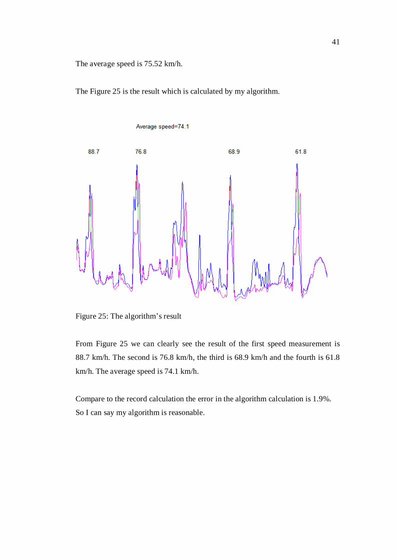
The average speed is 75.52 km/h.

The Figure 25 is the result which is calculated by my algorithm.

Figure 25: The algorithm‟s result

From Figure 25 we can clearly see the result of the first speed measurement is

88.7 km/h. The second is 76.8 km/h, the third is 68.9 km/h and the fourth is 61.8

km/h. The average speed is 74.1 km/h.

Compare to the record calculation the error in the algorithm calculation is 1.9%.

So I can say my algorithm is reasonable.

42

5 CONCLUSION

This project proves the feasibility of using the noise sensor network to detect the

vehicle speed on the highway. So this system can be improved to be used in real

life in the future.

The list over what has been done in the project includes the main steps as follows:

First, the feature of measured noise data has been analyzed.

Second, the algorithms to find the location of the missing data and fill them are

found, as well as the algorithm of the linear interpolation.

Third, I prove that it is necessary to use slope method in order to get rid of the

measurement ripples.

Fourth, the max/min/average speed calculated by the slope method is in the rea-

sonable range (for 80kph ramp, snowy day).

Fifth, the calibration shows that it can detect speed with good accuracy.

The algorithm will still be improved to calculate vehicle speed more accurate in

the future development as follows:

First, the algorithm of finding the time difference of the vehicle passing the two

nodes can be improved so that the calculation of the time difference is more accu-

rate. One way to improve the algorithm is that use a better algorithm to find two

more accurate slopes for each node.

Second, my algorithm is still not applicable for 2-way road. The purpose of my

detection is that only detect the vehicle speed which close to the node side. But

43

the nodes will both collect noise data from the 2 ways. After using this collected

data to draw the curve, it is difficult to distinguish the curve belong to which side

of the road. So in the future development we can still improve the algorithm to

detect the vehicle from 2-way road.

Third, my algorithm only can accurately detect first the speed of the vehicles

which close each other pass the nodes, because according to the curve only the

first vehicle‟s slope is clear. So in the future development we can improve the al-

gorithm to accurately detect all the speed of the vehicles which close each other.

44

REFERENCES

[1] Hakala, I., Kivela, I., Ihalainen, J., Luomala, J. & Gao, C. “Design of Low-

Cost Noise Measurement Sensor Network: Sensor Function Design”, In Proceed-

ing of Conference on Sensor Device Technologies and Applications

(SENSORDEVICES 2010), Venice, Italy, 18-23 July 2010.

[2] W. Morris, Ed., The American Heritage Dictionary of the English Language.

Houghton Mifflin, 2000.

[3] W. Boyes, Instrumentation Reference Book, 3rd ed., Butterworth-Heinemann,

2002

[4] D. Bies and C. Hansen, Engineering Noise Control, 4th ed., Spon Press, 2009.

[5] IEC 61672 Ed. 1.0, Electroacoustics-Soung level meters, Electroacoustics Std.,

2003

[6] Explaination for MATLAB linspace() function [online]. Available in www-

form :<URL: http://www.mathworks.com/help/techdoc/ref/linspace.html>

[7] Explaination for MATLAB fir() function [online]. Available in www-form:

<URL: http://www.mathworks.se/help/toolbox/signal/fir1.html>