Hurst phenomenon and fractional Gaussian noise made easy

Demetris Koutsoyiannis

Department of Water Resources, Faculty of Civil Engineering, National Technical University, Athens,

Heroon Polytechneiou 5, GR-157 80 Zographou, Greece

(dk@hydro.ntua.gr)

Abstract. The Hurst phenomenon, which characterises hydrological and other geophysical

time series, is formulated and studied in an easy manner in terms of the variance and

autocorrelation of a stochastic process on multiple temporal scales. In addition, a simple

explanation of the Hurst phenomenon based on the fluctuation of a hydrologic process upon

different temporal scales is presented. The stochastic process that was devised to represent the

Hurst phenomenon, i.e. the fractional Gaussian noise, is also studied on the same grounds.

Based on its studied properties, three simple and fast methods to generate fractional Gaussian

noise or good approximations of it are proposed.

Keywords. Hurst phenomenon; Fractional Gaussian noise; Persistence; Climate change.

Le phénomène Hurst et le bruit fractionnel gaussien rendus faciles dans leur

utilisation

Résumé. On formule et étudie d’une manière simple le phénomène Hurst, qui caractérise les

séries chronologiques en hydrologie et en géophysique, en termes de la variance et de l`

autocorrélation d`un processus stochastique considéré dans des échelles temporelles

multiples. De plus, on présente une explication simple du phénomène Hurst sur la base de la

fluctuation d`un processus hydrologique dans des échelles temporelles multiples. On étudie

aussi d’une manière analogue le bruit fractionnel gaussien qui constitue le processus

stochastique construit pour représenter le phénomène Hurst. Se basant sur les propriétés

étudiées de ce processus, on propose trois méthodes simples et rapides qui permettent de

générer du bruit fractionnel gaussien ou de bonnes approximations de ceci.

Mots clefs. Phénomène Hurst; Bruit fractionnel gaussien; Persistance; Changement climatique.

2

1. Introduction

While investigating the discharge time series of the Nile River in the framework of the design

of the Aswan High Dam, E. H. Hurst (1951) discovered a special behaviour of hydrologic and

other geophysical time series, which has become known as the ‘Hurst phenomenon’. This

behaviour is essentially the tendency of wet years to cluster into wet periods or of dry years to

cluster into drought periods. The term ‘Joseph effect’ introduced by Mandelbrot (1977, p.

248) has been used as an alternative for the same behaviour. Since its original discovery, the

Hurst phenomenon has been verified in several environmental quantities such as wind power

variations (Haslet and Raftery, 1989); global mean temperatures (Bloomfield, 1992); flows of

the river Nile (Eltahir, 1996); flows of the river Warta, Poland (Radziejewski and

Kundzewicz, 1997); monthly and daily inflows of Lake Maggiore, Italy (Montanari et al.,

1997); annual streamflow records across the continental United States (Vogel et al., 1998);

and indexes of North Atlantic Oscillation (Stephenson et al., 2000). In addition, the Hurst

phenomenon has gained new interest today due to its relation to climate changes (e.g. Evans,

1996).

Hurst (1951) formulated mathematically his discovery in terms of the so-called rescaled

range, which is a storage-related feature of a time series (Salas, 1993, p. 19.14; see also

Appendix A1). Several types of models such as fractional Gaussian noise (FGN) models

(Mandelbrot, 1965; Mandelbrot and Wallis, 1969a, b, c), fast fractional Gaussian noise

models (Mandelbrot, 1971), broken line models (Ditlevsen, 1971; Mejia et al., 1972),

fractional autoregressive integrated moving-average models (Hosking, 1981, 1984), and

symmetric moving average models based on a generalised autocovariance structure

(Koutsoyiannis, 2000) have been proposed to reproduce the Hurst phenomenon when

generating synthetic time series (see also Bras and Rodriguez-Iturbe, 1985, pp. 210-280).

Although hydrologists may agree that the Hurst phenomenon is inherent to hydrologic time

series, generally they prefer to use other, more convenient models to generate synthetic

hydrologic time series, such as autoregressive (AR) models, moving average (MA) models, or

combinations of the two (ARMA). For example, widespread stochastic hydrology packages

3

such as LAST (Lane and Frevert, 1990), SPIGOT (Grygier and Stedinger, 1990), and

CSUPAC1 (Salas, 1993) have not implemented any of the above listed types of models that

respect the Hurst phenomenon but rather they use AR, MA and ARMA models, which,

however, cannot reproduce the Hurst phenomenon. It is also known that this reproduction

may be essential in reservoir studies, especially in reservoirs performing overyear regulation

with draft close to the mean annual inflow (Bras and Rodriguez-Iturbe, 1985, p. 265).

There must be several reasons explaining this unwillingness to reproduce the Hurst

phenomenon in hydrologic practice. First, it is difficult to understand and explain, at least in

comparison to typical statistical behaviour of everyday life processes. Stochastic hydrology

texts (e.g. Yevjevich, 1972, pp. 131-172; Haan, 1977, p. 310; Kottegoda, 1980, pp. 184-203;

Bras and Rodriguez-Iturbe, 1985, pp. 210-265; Salas et al., 1988, p. 240; Salas, 1993) adopt

the original Hurst’s approach, which is in terms of range analysis of hydrologic series; as it is

shown in Appendix A1, the range analysis involves complexity and estimation problems. In

addition, the nature of the Hurst phenomenon has been the subject of debate, as discussed by

Bras and Rodriguez-Iturbe (1985, p. 214). Second, the algorithms that are used to generate

synthetic data series respecting the Hurst phenomenon are complicated. Third, the typical

models of this category have several weak points such as narrow type of autocorrelation

functions that they can preserve, and difficulties to preserve skewness and to perform in

multivariate problems.

Contrary to these, in this paper we attempt to show that the Hurst phenomenon is

essentially very simple to formulate, understand and reproduce in synthetic series – in some

aspects much simpler than the typical AR processes (some aspects of which are examined in

section 2), which, in addition, are not consistent with long historical hydroclimatic records

(section 3). We offer a mathematical formulation based on the relationship of the process

variance with the temporal scale of the process (section 4). In addition, we attempt to offer a

simple explanation of the Hurst phenomenon based on the fluctuation of a hydrologic process

upon different timescales (section 5). We also provide three simple methods to generate

fractional Gaussian noise or good approximations of it (section 6). Some mathematical

derivations are given in Appendix A2. Throughout this paper, we totally avoid using the range

4

concept and range analysis. To explain the reasons why we avoid the range concept and also

to link this presentation with the existing approaches of the Hurst phenomenon, we include

Appendix A1, which is devoted to range related topics.

Throughout the paper, the presentation of all issues is made as simple as possible; this is

done intentionally because the purpose of the paper is not to review the state of the art of the

research related to the Hurst phenomenon, nor to give the complete mathematical details of it

(for the latter see the comprehensive monograph by Beran, 1994) but rather (a) to assemble an

easy to understand mathematical basis and physical explanation of the phenomenon and (b) to

provide means for an easy implementation (e.g. using a spreadsheet package) of the methods,

both for estimation and simulation. To this aim, some original simple algorithms are provided.

2. Multiple timescale properties of typical stochastic processes

Hydrologic processes such as rainfall, runoff, evaporation, etc., are often modelled as

stationary stochastic processes in discrete time. Let us denote such a process Xi with i = 1, 2,

…, denoting discrete time (e.g. years). Further, let us denote its mean µ := E[Xi], its

autocovariance γj := Cov[Xi, Xi + j] and its autocorrelation ρj := Corr[Xi, Xi + j] = γj / γ0 ( j = 0,

±1, ±2, …).

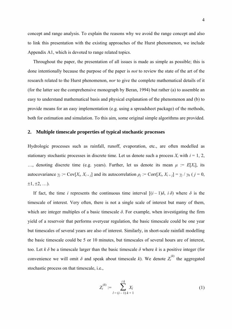
If fact, the time i represents the continuous time interval [(i – 1)δ, i δ) where δ is the

timescale of interest. Very often, there is not a single scale of interest but many of them,

which are integer multiples of a basic timescale δ. For example, when investigating the firm

yield of a reservoir that performs overyear regulation, the basic timescale could be one year

but timescales of several years are also of interest. Similarly, in short-scale rainfall modelling

the basic timescale could be 5 or 10 minutes, but timescales of several hours are of interest,

too. Let k δ be a timescale larger than the basic timescale δ where k is a positive integer (for

convenience we will omit δ and speak about timescale k). We denote Z (k)i the aggregated

stochastic process on that timescale, i.e.,

Z (k)i := ∑

l = (i – 1) k + 1

i k

Xl (1)

5

Obviously, for k = 1, Z (1)

i ≡ Xi; for k = 2, Z(2)1 := X1 + X2, Z

(2)2 := X3 + X4; for k = 3, Z

(3)1 := X1 +

X2 + X3, Z(3)2 := X4 + X5 + X6, etc. The statistical characteristics of Z

(k)i for any timescale k can

be derived from those of Xi. For example, the mean is

E[Z (k)

i ] = k µ (2)

whilst the variance and autocovariance (or autocorrelation) is more difficult to derive as it

depends on the specific structure of γj (or ρj). A general expression that gives the covariance at

any scale k in terms of that at the basic scale can be found using (1); this is

γ (k)j := Cov[Z

(k)i , Z

(k)i + j] = ∑

l = 1

k

∑m = j k + 1

(j + 1) k

γm – l, j = 0, ±1, ±2, … (3)

The autocovariance is related to the power spectrum of the process, which in general case

is the discrete Fourier transform (DFT; also termed the inverse finite Fourier transform) of γj

(e.g., Papoulis, 1991, pp. 118, 333; Bloomfield, 1976, pp. 46-49; Debnath, 1995, pp. 265-

266), that is

s (k) γ (ω) := 2 γ

(k) 0 + 4 ∑

j = 1

∞ γ

(k) j cos (2 π j ω) = 2 ∑

j = –∞

∞ γ

(k) j cos (2 π j ω) (4)

Because γj is an even function of j (i.e., γj = γ–j), the DFT in (4) is a cosine transform; as

usually we have assumed in (4) that the frequency ω ranges in [0, 1/2], so that γj is determined

in terms of sγ(ω) by the finite Fourier transform

γ (k) j = ⌡⌠

0

1/2

s (k) γ (ω) cos (2 π j ω) dω (5)

Before we study the process known as fractional Gaussian noise (FGN), which respects the

Hurst phenomenon (this will be done in section 4), it may be a good idea to refer to two of the

simplest stochastic models that we are more familiar with.

6

The first is white the noise, in which different Xi are independent identically distributed

random variables, so that γj = 0 (and ρj = 0) for j ≠ 0. Apparently then, the aggregated process

will have variance

γ (k) 0 := Var[Z

(k)i ] = k γ0 (6)

autocovariance γ (k) j = 0 and autocorrelation ρ

(k) j = 0. From (4) we easily find that its power

spectrum is constant, independent of the frequency ω, i.e.,

s (k) γ (ω) / γ

(k) 0 = 2 (7)

In fact, the constant value of the power spectrum, i.e., the presence of all frequencies ω with

the same magnitude, has been the reason for the term ‘white noise’.

As a second example, let us assume that the process Xi at the basic timescale is the simpler

possible process with some dependence of the current value on previous ones, also termed

memory of the process. This is the autoregressive process of order 1 (AR(1)) and the

dependence is expressed by

Xi = ρ Xi – 1 + Vi (8)

where ρ is the lag one autocorrelation coefficient (–1 < ρ < 1) and Vi (i = 1, 2, …) are

innovations, i.e. independent identically distributed random variables with mean (1 – ρ) µ and

variance (1 – ρ2) γ0. The process is also termed Markovian because the dependence of the

current variable Xi on the previous variable Xi – 1 suffices to express completely the

dependence of the present on the past. The autocorrelation of Xi is

ρj := Corr[Xi, Xi + j] = ρ| j| (9)

Combining (9) and (3) after some algebra we find for the aggregated process

γ (k) 0 = γ0

k (1 – ρ2) – 2ρ (1 – ρk) (1 – ρ)2 (10)

γ (k) j = γ0

ρk j – k + 1 (1 – ρk)2

(1 – ρ)2 , j ≥ 1 (11)

7

and thus the autocorrelation is

ρ (k)j = ρ

(k)1 ρ

k (j – 1) , j ≥ 1 (12)

with

ρ (k)1 =

ρ (1 – ρk)2

k (1 – ρ2) – 2ρ (1 – ρk) (13)

By comparing (12)-(13) with (9) we conclude that Z (k)i is no longer a Markovian process but a

more complicated one (in fact (12) corresponds to an ARMA(1, 1) process; Box et al., 1994,

p. 81). In other words, the simple AR(1) process is an AR(1) process only on its basic

timescale, whereas it becomes more complicated on aggregated timescales.

Τhe power spectrum of the aggregated process Z (k)i can be found by adapting the power

spectrum of the AR(1) process (Box et al., 1994, p. 58). After algebraic manipulations we get

s (k) γ (ω) / γ

(k) 0 = 2 + 4 ρ

(k) 1

cos (2 π ω) – ρk 1 + ρ2k – 2 ρk cos (2 π ω) (14)

For relatively small k, this gives a characteristic inverse S-shaped power spectrum that

corresponds to a short memory process.

For a large aggregated timescale k, the numerator of (10) is dominated by the first term and

the variance of the aggregated process becomes

γ (k) 0 ≈ k

1 + ρ1 – ρ γ0 (15)

i.e., it becomes proportional to the timescale k, similarly as in the white noise process. Also,

from (13) we observe that ρ (k) 1 becomes small, as does ρ

(k) j . Consequently, from (14) we

conclude that the power spectrum becomes sγ(ω) / γ0 = 2, which characterises white noise.

In conclusion, if the process of interest is Markovian at the basic timescale, it tends to

white noise for progressively increasing timescales. (In fact this happens with higher order

AR and ARMA processes as well).

8

3. Some real world examples

Empirical evidence suggests that long historical hydroclimatic series may exhibit a behaviour

very different from that implied by simple models such as the above described, or even more

complicated models such as the ARMA ones. To demonstrate this we use two real world

examples. The first is the most intensively studied series, which also led to the discovery of

the Hurst phenomenon (Hurst, 1951): the series of the annual minimum water level of the

Nile river for the years 622 to 1284 A.D. (663 observations), measured at the Roda Nilometer

near Cairo (Toussoun, 1925, p. 366-385; Beran, 1994). The data is available from

http://lib.stat.cmu.edu/S/beran. The second example is an even longer record; the series of

standardised tree ring widths from a paleoclimatology study at Mammoth Creek, Utah, for the

years 0-1989 (1990 values; Year 0 in fact stands for 1 B.C. as the calendar does not contain

Year 0). The data, originated from pine trees at elevation 2590 m, latitude 37:39, longitude

112:40 (Graybill, 1990) is available from ftp://ftp.ngdc.noaa.gov/paleo/treering/chronologies/

asciifiles/usawest/ut509.crn.

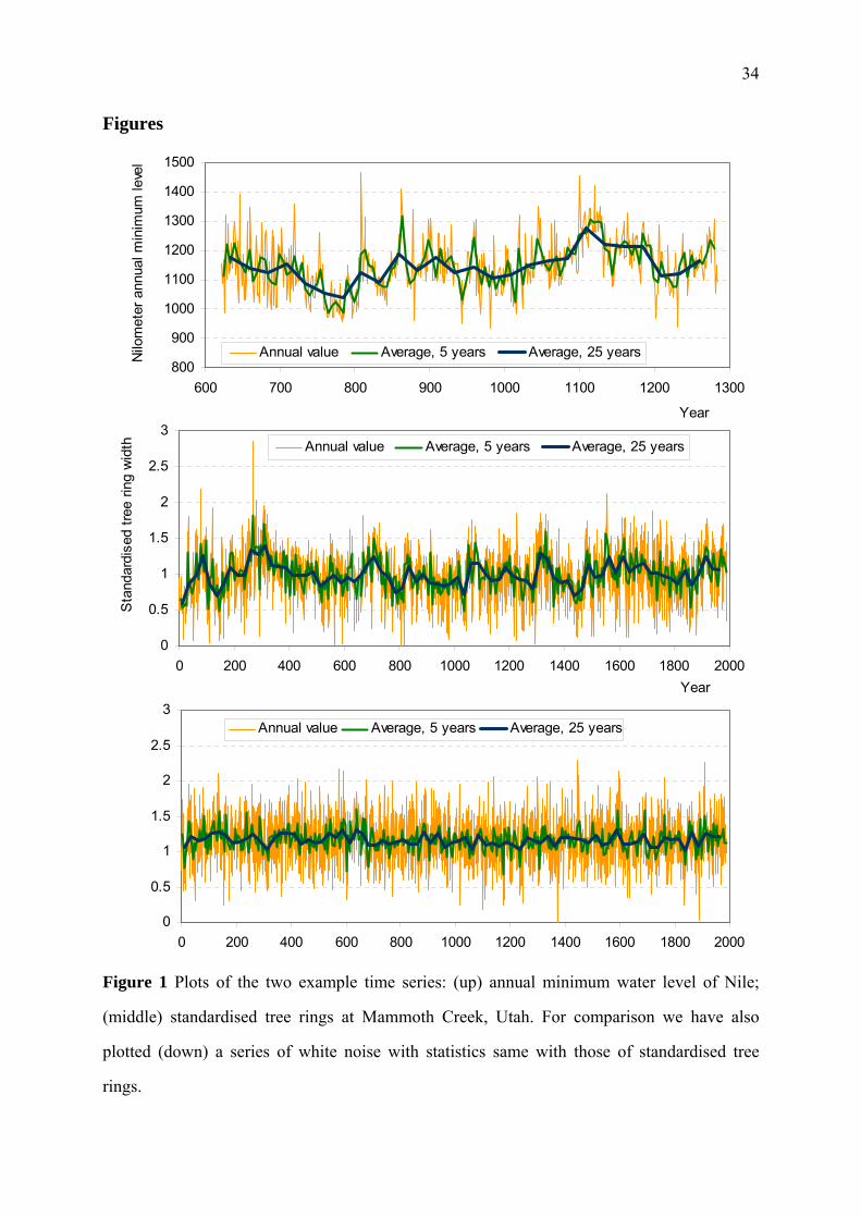
In Figure 1 we have plotted the data values versus time for both example data sets. In

addition, we have plotted the 5-year and 25-year averages, which represent the aggregated

processes at timescales k = 5 and 25, respectively. For comparison we have also plotted a

series of white noise with statistics same to those of standardised tree rings. We can observe

that fluctuations of the aggregated processes, especially for k = 25, are much greater in the

real world time series than in the white noise series. These fluctuations could be taken as

nonstationarities, that is, deterministic rising or falling trends that last 100-200 or more years.

For example, if one had available only the data of the period 700-800 of either of the two time

series, he or she would speak about a deterministic falling trend; similarly, one would speak

about a regular rising trend of the Nile level between the years 1000-1100 or of the Utah

series between years 100-300. However, the complete pictures for both series suggest that

these trends are parts of large-scale random fluctuations rather than deterministic trends.

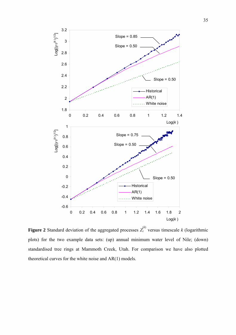
In Figure 2 we have plotted on logarithmic diagrams the standard deviation of the

aggregated processes versus timescale k for the two example data sets. For comparison we

9

have also plotted theoretical curves for the white noise and AR(1) models (equations (6) and

(10), respectively). Clearly, the plots of both series are almost straight lines on the logarithmic

diagram with slopes 0.75-0.85. Both the white noise and the AR(1) models result in a slope

equal to 0.5, significantly departing from historical data.

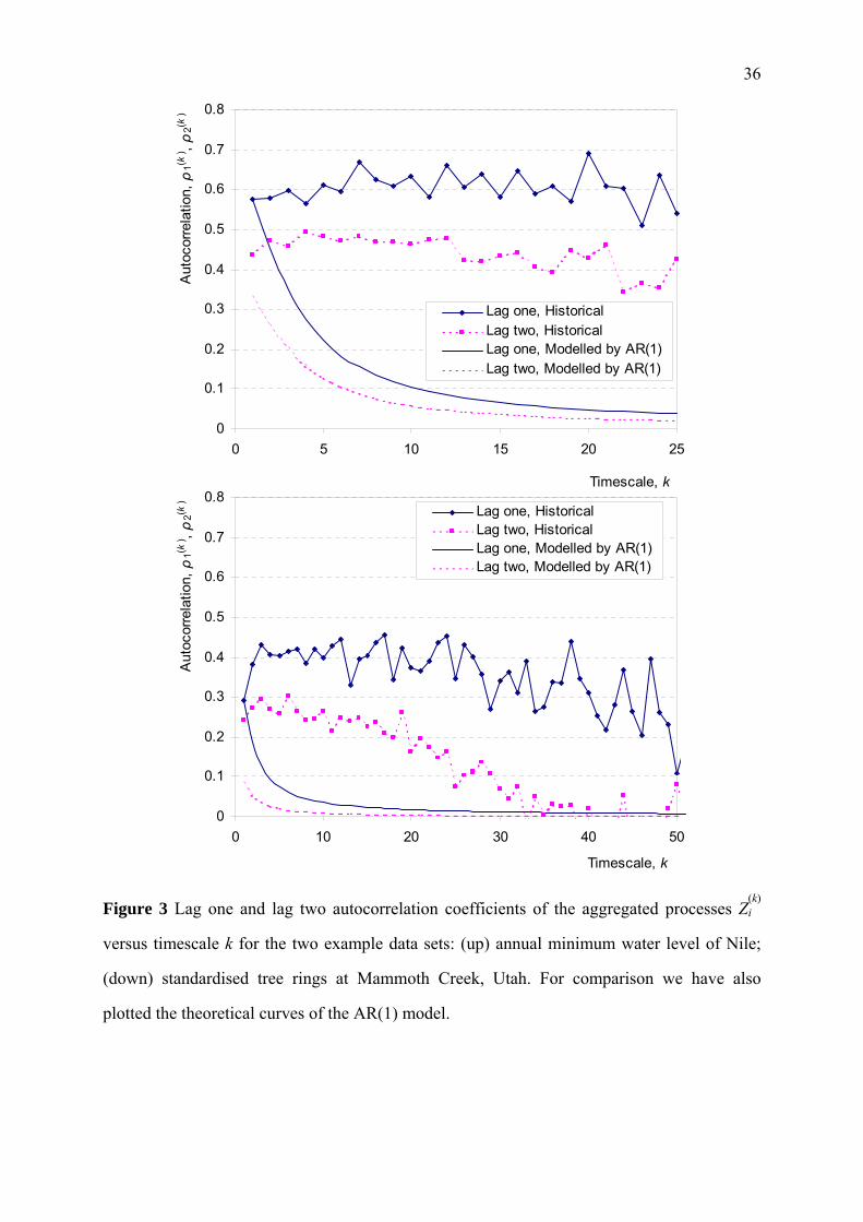
Furthermore, in Figure 3 we have plotted the autocorrelation coefficients of the aggregated

processes for lag one and lag two, versus the timescale k, for the two example data sets. For

comparison we have also plotted theoretical curves for the AR(1) model. The empirical

autocorrelation coefficients are almost constant for all timescales whereas the AR(1) model

results in autocorrelations that drop down to zero for large timescales.

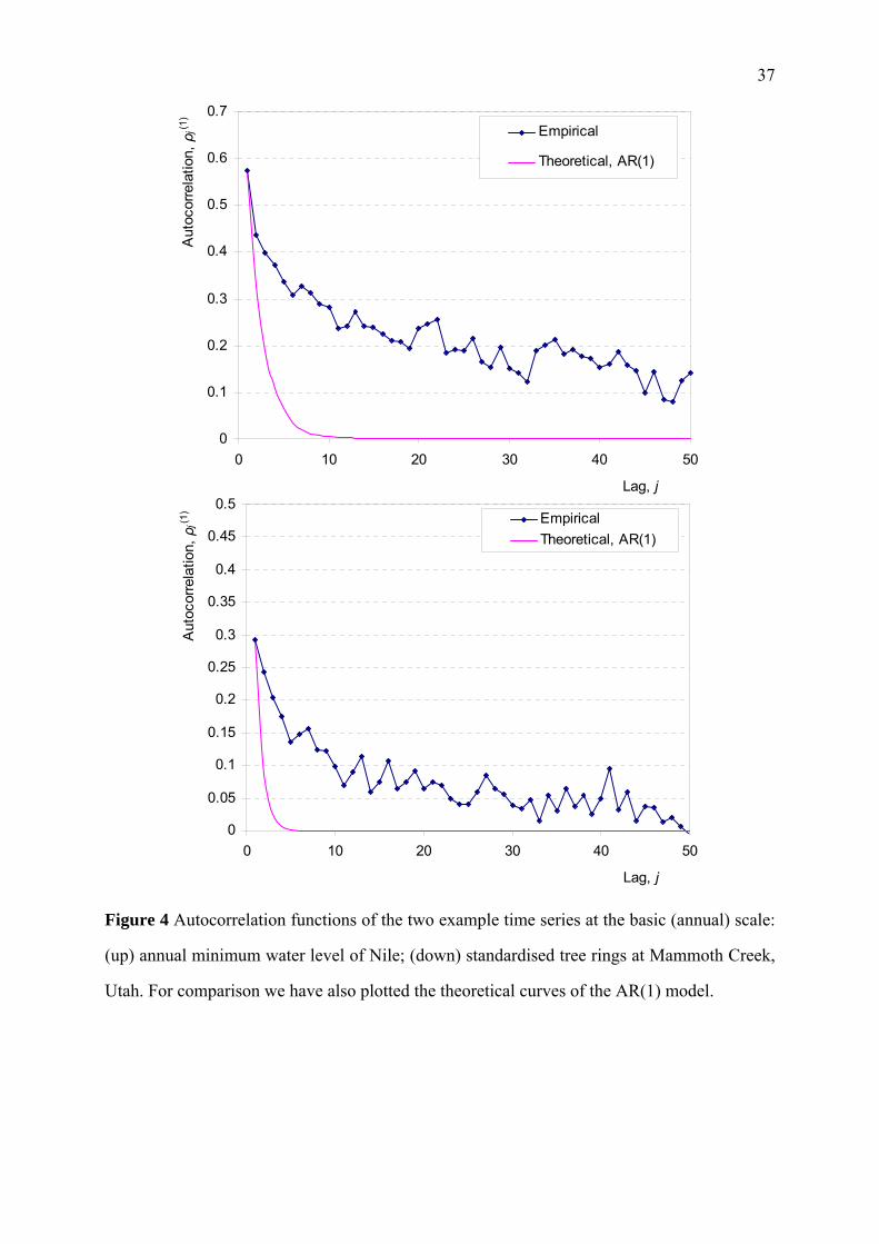
Finally, in Figure 4 we have plotted the autocorrelation functions of the two example time

series at the basic (annual) timescale along with the theoretical curves of the AR(1) model.

Clearly, the curves of the AR(1) vanish off for lags 4-10 whereas the curves of the historical

series are fat tailed and do not vanish for lags as high as 50. In conclusion, this discussion

provides some further evidence, using a multiple-timescale approach, to the well-known fact

that the AR(1) model is inconsistent with hydroclimatic reality (a similar conclusion can be

drawn for more complex processes of the ARMA type).

4. The fractional Gaussian noise process

To restore consistency with reality, Mandelbrot (1965) introduced the process known as

fractional Gaussian noise (FGN). The FGN process can be defined in discrete time (which is

our scope here) in a manner similar to that used in continuous time (e.g. Saupe, 1988, p. 82;

Abry et al., 1995). Specifically, the FGN process can be defined as a process satisfying the

condition

(Z (k)

i – k µ) =d ⎝⎜⎛

⎠⎟⎞k

l

H

(Z (l)j – l µ) (16)

where the symbol =d stands for equality in (finite dimensional joint) distribution and H is a

positive constant (0 < H < 1) known as the Hurst exponent (or coefficient). Equation (16) is

10

valid for any integer i and j (that is, the process is stationary) and any timescales k and l. As a

consequence, for i = j = l = 1 we get

γ (k)0 := Var[Z

(k)i ] = k2H γ0 (17)

Thus, the standard deviation is a power law of k with exponent H, which agrees with the

observation on the real world cases of section 3. The extremely simple relation (17) can serve

as the basis for estimating H (Montanari et al., 1997).

It is easy then to show (see Appendix A2) that, for any aggregated timescale k, the

autocovariance function is independent of k, again agreeing with the observation of section 3.

Specifically, it is given by

ρ (k)j = ρj = (1 / 2) [(j + 1)2H + (j – 1)2H ] – j2H, j > 0 (18)

Apart from small j, this function is very well approximated by

ρ (k)j = ρj = Η (2 Η – 1) j 2 H – 2 (19)

which shows that autocorrelation is a power function of lag.

Notably, (18) can be obtained from a continuous time process Ξ(t) with autocorrelation

Cov[Ξ(t), Ξ(t + τ)] = a τ 2 H – 2 (with constant a = Η (2 Η – 1) γ0), by discretising the process

using time intervals of any length δ and taking as Xi the average of Ξ(t) in the interval [i δ,

(i + 1) δ]. This enables an approximate calculation of the power spectrum of the process as

s (k) γ (ω) = 2 ∑

j = –∞

∞ γ

(k) j cos (2 π j ω) ≈ 4 ⌡⌠

0

∞ a τ 2 H – 2 cos (2 π τ ω) dτ (20)

which results in the approximation s (k)γ (ω) ≈ a΄ ω1 – 2 H. To find the constant a΄ so as to

preserve exactly the process variance γ0 we use (5) to get

γ (k) 0 = ⌡⌠

0

1/2

a΄ ω1 – 2 H dω =

a΄(2 – 2 H) 22 – 2 H (21)

from which we finally obtain

11

s (k)γ (ω) / γ

(k) 0 ≈ 4 (1 – H) (2 ω)1 – 2 H (22)

which is a power law of the frequency ω.

Similarly to the AR(1) process, which uses one single parameter ρ to express the

correlation structure of the process, the FGN process uses again one parameter, the Hurst

exponent H. Therefore we can characterise the FGN process as a simplified model of reality,

noting that it is much more effective in representing hydroclimatic series than the AR(1)

process. A generalised and comprehensive family of processes, which can have a larger

number of parameters and incorporates both the FGN and the ARMA processes, has been

introduced by Koutsoyiannis (2000).

Comparing the FGN process to the AR(1) process in terms of the expressions of the basic

statistical properties at multiple timescales, we observe that the former is rather simpler than

the latter. Thus, the expression of the process variance at any scale k (equation (17)) is much

simpler that that of AR(1) (equation (10)). Similarly, the expression of the process correlation

at any scale k (equation (18))) is simpler that that of AR(1) (equations (12) and (13)).

5. A physical explanation

We are very familiar with a white noise process, a process where each event is totally

independent from previous ones, e.g., a sequence of outcomes of consecutive throws of dice.

Under the assumption of a stable climate, the maximum flood peaks of consecutive years

form a white noise process, as well, as there is no stochastic dependence between flood events

belonging to different hydrologic years. We are less familiar with processes that have some

memory, but we can understand Markovian (e.g., AR(1)) processes. For example, Yevjevich

(1972, p. 27) explained that the annual flow series is dependent and follows a Markovian

process. To show this, Yevjevich assumed that the catchment is stimulated by an effective

precipitation process that is white noise and that the water carry-over from year to year is

ruled by a groundwater recession curve that is an exponential function of time.

However, the Hurst phenomenon and the related FGN process are more difficult to

understand. Mesa and Poveda (1993) classify the Hurst phenomenon as one of the most

12

important unsolved problems in hydrology and state that “something quite dramatic must be

happening from a physical point of view”. The FGN process is very different from a

Markovian process in that it implies a fat tailed autocorrelation function. For instance, if the

Hurst coefficient is 0.85, as in the Nile example given in section 3, then the autocorrelation

for lag 100 (years) is as high as 0.15, whereas if the process were Markovian the

autocorrelation would be practically zero even for lags 10 times less. Does the explanation of

this behaviour of natural systems, such as Nile’s water level or Mammoth Creek’s tree ring

widths, rest on the self-organised criticality principle (Bak, 1996, pp. 21, 22, 31, 37), i.e., a

cooperative behaviour, where the different items of large systems act together in some

concerted way? Or, is it rest on monotonic deterministic trends (Bhattachara et al., 1983),

which can explain mathematically this behaviour? Or, is there any natural mechanism

inducing a long memory to the system, which is responsible for the high autocorrelation for a

lag of 100 years or more?

The author’s explanation is much simpler and relies upon an ‘absence of memory’ concept

rather than a ‘long-term memory’ concept. That is, we set the hypothesis that not only does

the system ‘disremember’ what was the value of the process 100 years (or more) ago, but it

further ‘forgets’ what the process mean at that time was. This explanation is consistence with

the assertion of the National Research Council (1991, p. 21) that climate “changes irregularly,

for unknown reasons, on all timescales”. The idea of irregular sporadic changes in the mean

of the process appeared also in Salas and Boes (1980), but not in connection with FGN and

not in the setting of multiple timescales. The idea of composite random processes with two

timescales of fluctuation appeared in Vanmarcke (1983, p. 225). For more mathematical

explanations of FGN the interested reader is referenced to Beran (1994, pp. 14-20).

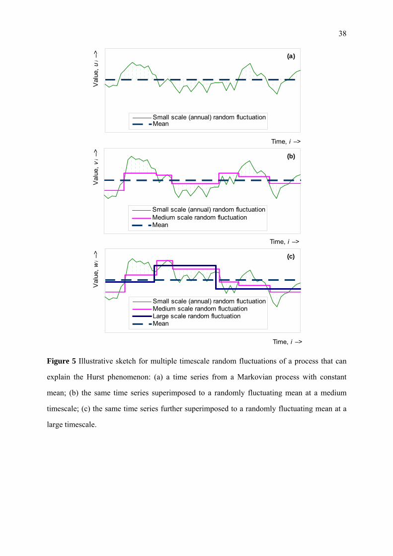
To demonstrate our explanation let us start with a (easy to understand) Markovian process

Ui, like the one graphically demonstrated in Figure 5(a), with mean µ := E[Ui], variance γ0 and

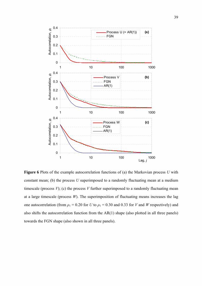
lag one autocorrelation coefficient ρ = 0.20. The autocorrelation function (given by (9)) for

lags up to 1000 is shown in Figure 6(a) along with the autocorrelation function for the FGN

process with same lag one autocorrelation coefficient (0.20). We observe the large difference

13

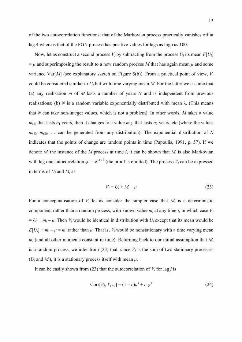
of the two autocorrelation functions: that of the Markovian process practically vanishes off at

lag 4 whereas that of the FGN process has positive values for lags as high as 100.

Now, let as construct a second process Vi by subtracting from the process Ui its mean E[Ui]

= µ and superimposing the result to a new random process M that has again mean µ and some

variance Var[M] (see explanatory sketch on Figure 5(b)). From a practical point of view, Vi

could be considered similar to Ui but with time varying mean M. For the latter we assume that

(a) any realisation m of M lasts a number of years N and is independent from previous

realisations; (b) N is a random variable exponentially distributed with mean λ. (This means

that N can take non-integer values, which is not a problem). In other words, M takes a value

m(1) that lasts n1 years, then it changes to a value m(2) that lasts n2 years, etc (where the values

m(1), m(2), … can be generated from any distribution). The exponential distribution of N

indicates that the points of change are random points in time (Papoulis, 1991, p. 57). If we

denote Mi the instance of the M process at time i, it can be shown that Mi is also Markovian

with lag one autocorrelation φ := e–1 / λ (the proof is omitted). The process Vi can be expressed

in terms of Ui and Mi as

Vi = Ui + Mi – µ (23)

For a conceptualisation of Vi let as consider the simpler case that Mi is a deterministic

component, rather than a random process, with known value mi at any time i, in which case Vi

= Ui + mi – µ. Then Vi would be identical in distribution with Ui except that its mean would be

E[Ui] + mi – µ = mi rather than µ. That is, Vi would be nonstationary with a time varying mean

mi (and all other moments constant in time). Returning back to our initial assumption that Mi

is a random process, we infer from (23) that, since Vi is the sum of two stationary processes

(Ui and Mi), it is a stationary process itself with mean µ.

It can be easily shown from (23) that the autocorrelation of Vi for lag j is

Corr[Vi, Vi + j] = (1 – c)ρ j + c φ j (24)

14

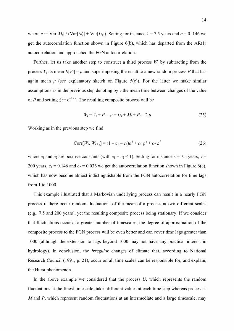
where c := Var[Mi] / (Var[Mi] + Var[Ui]). Setting for instance λ = 7.5 years and c = 0. 146 we

get the autocorrelation function shown in Figure 6(b), which has departed from the AR(1)

autocorrelation and approached the FGN autocorrelation.

Further, let us take another step to construct a third process Wi by subtracting from the

process Vi its mean E[Vi] = µ and superimposing the result to a new random process P that has

again mean µ (see explanatory sketch on Figure 5(c)). For the latter we make similar

assumptions as in the previous step denoting by ν the mean time between changes of the value

of P and setting ξ := e–1 / ν. The resulting composite process will be

Wi = Vi + Pi – µ = Ui + Mi + Pi – 2 µ (25)

Working as in the previous step we find

Corr[Wi, Wi + j] = (1 – c1 – c2)ρ j + c1 φ j + c2 ξ j (26)

where c1 and c2 are positive constants (with c1 + c2 < 1). Setting for instance λ = 7.5 years, ν =

200 years, c1 = 0.146 and c2 = 0.036 we get the autocorrelation function shown in Figure 6(c),

which has now become almost indistinguishable from the FGN autocorrelation for time lags

from 1 to 1000.

This example illustrated that a Markovian underlying process can result in a nearly FGN

process if there occur random fluctuations of the mean of a process at two different scales

(e.g., 7.5 and 200 years), yet the resulting composite process being stationary. If we consider

that fluctuations occur at a greater number of timescales, the degree of approximation of the

composite process to the FGN process will be even better and can cover time lags greater than

1000 (although the extension to lags beyond 1000 may not have any practical interest in

hydrology). In conclusion, the irregular changes of climate that, according to National

Research Council (1991, p. 21), occur on all time scales can be responsible for, and explain,

the Hurst phenomenon.

In the above example we considered that the process U, which represents the random

fluctuations at the finest timescale, takes different values at each time step whereas processes

M and P, which represent random fluctuations at an intermediate and a large timescale, may

15

have the same value for several time steps. This assumption was done for the sake of a

simpler demonstration and it is not a structural assumption at all; without any change we

could assume that M and P take different values at each time step, provided that their

covariance structure remains Markovian with the same autocorrelation.

The above explanation may seem similar (from a practical point of view) to that by Klemes

(1974), who attributed the Hurst phenomenon to non-stationary means. However, there is a

fundamental difference here. As shown in the above analysis, we do not assume that means

are nonstationary but rather, they are randomly varying at several scales. Nonstationarity of

the mean would be the case if there existed a deterministic function expressing the mean as a

function of time. Even though in some hydrologic texts (e.g., Kottegoda, 1980, p. 26), the

falling or rising large-scale trends, traced in several hydrological time series, are classified as

‘deterministic components’ and are expressed as, say, linear functions of time, it is the

author’s opinion that these trends are not deterministic at all. For example, (as already

discussed in section 3) the 25-year moving averages on the time series of Figure 1 indicate

that there exist falling and rising large-scale trends but they follow an irregular random

pattern rather than a regular deterministic one.

The conclusion of the above demonstration is that the nonstationarity notion is not

necessary at all to explain the Hurst phenomenon. A stationary process can capture the Hurst

effect and this agrees with Mandelbrot’s notion. However, our explanation is contrary to the

concept of long memory; the high autocorrelations appearing for high lags do not indicate

long memory but they are a consequence of the large-scale random fluctuations as

demonstrated with our simple example.

6. Simple algorithms to generate fractional Gaussian noise

As we have discussed in the introduction, several algorithms have been proposed to generate

time series that respect the Hurst phenomenon. For some of these, the source code is widely

available (e.g., the Splus programs by Beran, 1994, pp. 218-237). However, some of the

known algorithms are not so simple both in understanding and implementation. Below we

propose three much simpler algorithms that can be applied even in a spreadsheet environment.

16

These are based on the above-discussed properties of FGN and can be used to provide

approximations of FGN good for practical hydrological purposes. In principle, all algorithms

provided can be tuned to become as accurate as demanded. However, here we preferred to

give emphasis to simplicity rather than accuracy. Theoretically, the algorithms can perform

for any value of the Hurst exponent H in the interval (0, 1). However we have tested them on

the subinterval (0.5, 1), which corresponds to the Hurst phenomenon (when H < 0.5 the

autocorrelation function becomes negative for any lag, a case that is not met in hydrologic

practice).

6.1 A multiple timescale fluctuation approach

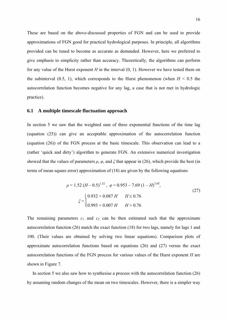
In section 5 we saw that the weighted sum of three exponential functions of the time lag

(equation (25)) can give an acceptable approximation of the autocorrelation function

(equation (26)) of the FGN process at the basic timescale. This observation can lead to a

(rather ‘quick and dirty’) algorithm to generate FGN. An extensive numerical investigation

showed that the values of parameters ρ, φ, and ξ that appear in (26), which provide the best (in

terms of mean square error) approximation of (18) are given by the following equations

ρ = 1.52 (H – 0.5)1.32 , φ = 0.953 – 7.69 (1 – H)3.85, (27)

ξ = ⎩⎪⎨⎪⎧0.932 + 0.087 H H ≤ 0.76

0.993 + 0.007 H H > 0.76

The remaining parameters c1 and c2 can be then estimated such that the approximate

autocorrelation function (26) match the exact function (18) for two lags, namely for lags 1 and

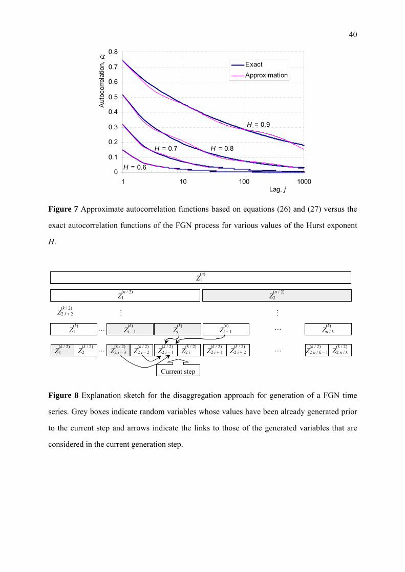
100. (Their values are obtained by solving two linear equations). Comparison plots of

approximate autocorrelation functions based on equations (26) and (27) versus the exact

autocorrelation functions of the FGN process for various values of the Hurst exponent H are

shown in Figure 7.

In section 5 we also saw how to synthesise a process with the autocorrelation function (26)

by assuming random changes of the mean on two timescales. However, there is a simpler way

17

to utilise (26) for generation of a time series. Specifically, (26) represents the sum of three

independent AR(1) processes like that in (8), with lag one correlation coefficients ρ, φ, and ξ,

and variances (1 – c1 – c2) γ0, c1 γ0, and c2 γ0, respectively.

It must be mentioned that this algorithm is based essentially on the same principle with the

fast fractional Gaussian noise (FFGN) algorithm (Mandelbrot, 1971); the differences are that

it uses only 3 AR(1) components, much less than the FFGN, and the parameters of the

algorithm are determined by the much simpler equation (27). Although the achieved

approximation with the 3 AR(1) components is sufficient in practice for lags as high as 1000,

it can be improved by increasing the number of the AR(1) components to 4, 5, etc. However,

(27) will be not applicable then and the variances and lag one autocorrelations of the

components must be estimated by minimising the mean squared departure of the composite

autocorrelation function from that of the FGN process.

6.2 A disaggregation approach

The simple expressions of the statistics of the aggregated FGN process make possible a

disaggregation approach for generating a time series of a FGN process. Specifically, let us

assume that the desired length n of the synthetic series to be generated is 2m where m is an

integer (e.g., n = 2, 4, 8, 16, …; if n is not a power of 2 we can increase it to the next power of

2 and then discard the redundant generated items). We first generate the single value of Z(n)1

knowing that its variance is (from (17)) n2H γ0. Then we disaggregate Z(n)1 into two variables at

the timescale n / 2, i.e. Z(n / 2)1 and Z

(n / 2)2 and we proceed this way until the series Z

(1)1 ≡ X1, …,

Z(1)n ≡ Xn is generated (see explanatory sketch on Figure 8).

The disaggregation algorithm that we propose reminds the midpoint displacement method

(Saupe, 1988, p. 84) but is more accurate. It is based on a disaggregation technique introduced

by Koutsoyiannis (2001). Since it is an induction technique it suffices to describe one step of

the method application. Let us assume that we have completed the generation at the timescale

k ≤ n and we are generating the time series at the next timescale k / 2 (see Figure 8). We

consider the generation step in which we disaggregate the higher-level amount Z(k)i (1 < i <

n / k) into two lower-level amounts Z(k / 2)2 i – 1 and Z

(k / 2)2 i such that

18

Z(k / 2)2 i – 1 + Z

(k / 2)2 i = Z

(k)i (28)

Thus, it suffices to generate Z(k / 2)2 i – 1 and then obtain Z

(k / 2)2 i from (28). At this generation step we

have available the already generated values of previous lower-level time steps, i.e., Z(k / 2)1 , …,

Z(k / 2)2 i – 2 and of next higher-level time steps, i.e., Z

(k)i + 1, …, Z

(k)n / k (see explanatory sketch on

Figure 8). Theoretically, it is necessary to preserve the correlations of Z(k / 2)2 i – 1 with all previous

lower-level variables and all next higher-level variables. However, we can get a very good

approximation if we consider correlations with only one higher-level time step behind and one

ahead. Under this simplification, Z(k / 2)2 i – 1 can be generated from the linear relationship

Z(k / 2)2 i – 1 = a2Z

(k / 2)2 i – 3 + a1Z

(k / 2)2 i – 2 + b0 Z

(k)i + b1 Z

(k)i + 1 + V (29)

where a2, a1, b0 and b1 are parameters to be estimated and V is innovation whose variance has

to be estimated, too. All unknown parameters can be estimated in terms of correlations of the

form Corr[Z(k / 2)2 i – 1, Z

(k / 2)2 i – 1 + j] = ρj where ρj is given by (18). Specifically, applying the

methodology by Koutsoyiannis (2001) we find

⎣⎢⎢⎡

⎦⎥⎥⎤

a2

a1

b0

b1

=

⎣⎢⎢⎡

⎦⎥⎥⎤

1 ρ1 ρ2 + ρ3 ρ4 + ρ5

ρ1 1 ρ1 + ρ2 ρ3 + ρ4

ρ2 + ρ3 ρ1 + ρ2 2(1 + ρ1) ρ1 + 2ρ2 + ρ3

ρ4 + ρ5 ρ3 + ρ4 ρ1 + 2ρ2 + ρ3 2(1 + ρ1)

–1

⎣⎢⎢⎡

⎦⎥⎥⎤

ρ2

ρ1

1 + ρ1

ρ2 + ρ3

(30)

and

Var[V] = γ (k / 2)0 (1 – [ρ2, ρ1, 1 + ρ1, ρ2 + ρ3] [a2, a1, b0, b1]T ) (31)

where the superscript T denotes the transpose of a vector.

All parameters are independent of i and k and therefore they can be used in all steps. When

i = 1 there are no previous time steps and thus the first two rows and columns of the above

matrix and vectors are eliminated. Similarly, when i = n / k, there is no next time step and thus

the last row and column of the above matrix and vectors are eliminated. The sequences of

previous and past variables that are considered for generating each lower-level variable, and

the related parameters, can be directly expanded, to increase the accuracy of the method.

19

However, as we will see in section 6.4, the above minimal configuration of the method gives

satisfactory results.

6.3 A symmetric moving average approach

Koutsoyiannis (2000) introduced the so call symmetric moving average (SMA) generating

scheme that can be used to generate any kind of stochastic process with any autocorrelation

structure or power spectrum. Like the conventional (backward) moving average (MA)

process, the SMA scheme transforms a white noise sequence Vi into a process with

autocorrelation by taking the weighted average of a number of Vi. In the SMA process the

weights aj are symmetric about a centre (a0) that corresponds to the variable Vi, i.e.,

Xi = ∑j = –q

q a|j| Vi + j = aq Vi – q + … + a1 Vi – 1 + a0 Vi + a1 Vi + 1 + … + aq Vi + q (32)

where q theoretically is infinity but in practice can be restricted to a finite number, as the

sequence of weights aj tends to zero for increasing j. The autocovariance implied by (32) is

γj = ∑l = –q

q – j a|l| a|j + l|, j = 0, 1, 2, … (33)

Koutsoyiannis (2000) also showed that the discrete Fourier transform sa(ω) of the aj

sequence is related to the power spectrum of the process sγ(ω) by

sa(ω) = 2 sγ(ω) (34)

This enables the direct calculation of sa(ω), which in the case of FGN, given (22), will be

sa(ω) ≈ 2 (2 – 2 H) γ0 (2 ω)0.5 – H (35)

Comparing (22) and (35) we observe that sa(ω) is approximately equal to the power spectrum

of another FGN process with Hurst exponent H΄ = (Η + 0.5) / 2 and variance

[ 2 – 2 H / (1.5 – H)] γ0. Consequently, we can use (18) to approximate the inverse Fourier

transform of sa(ω), i.e., the sequence of aj itself:

20

aj ≈ (2 – 2 H) γ0

3 – 2H [(j + 1)H + 0.5 + (j – 1)H + 0.5 – 2 jH + 0.5], j > 0 (36)

In conclusion, the generation scheme (32) with coefficients aj determined from (36) can

lead to a very easy algorithm for generating FGN. This method can also preserve the process

skewness ξΧ by appropriately choosing the skewness of the white noise ξV. The relevant

equations for the statistics of Vi, which are direct consequences of (32), are

⎝⎜⎜⎛

⎠⎟⎟⎞

a0 + 2 ∑j = 1

s aj E[Vi] = µ, Var[Vi] = 1,

⎝⎜⎜⎛

⎠⎟⎟⎞

a03+ 2 ∑

j = 1

q aj

3 ξV = ξΧ γ0 3/2 (37)

Given that the weights aj are q + 1 in total, the model can preserve the first q + 1 terms of

the autocovariance γj of the process Xi. Thus, the number q must be chosen at least equal to

the desired number of autocorrelation coefficients m that are to be preserved. In addition, the

ignored terms aj beyond aq must not exceed an acceptable tolerance β γ0. These two

conditions in combination with (19) and (36) result in

q ≥ max⎣⎢⎡

⎦⎥⎤

m‚ ⎝⎜⎛

⎠⎟⎞2 β

H2 – 0.25

1 / (H – 1.5)

(38)

The number q can be very large (on the order of thousands to hundred of thousands) if H is

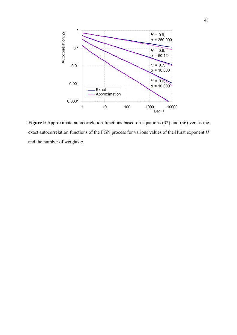
large (e.g. > 0.9) and β is small (e.g. < 0.001). Approximate autocorrelation functions for lags

up to m = 10 000 based on equations (32) and (36) versus the exact autocorrelation functions

of the FGN process for various values of the Hurst exponent H and the number of weights q

are shown in Figure 9.

The accuracy of the method depends on the number q. However, even when q → ∞ the

method does not become exact because of the approximate character of (36). Although more

accurate estimates the aj series can be obtained numerically by a method by Koutsoyiannis

(2000), the estimates given by (36) are sufficiently accurate for practice. This is verified in

Figure 9 where theoretical and approximate autocorrelation functions are almost

indistinguishable.

21

6.4 Demonstration of the methods

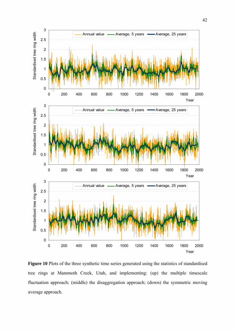
The three proposed methods for generating FGN are demonstrated by synthesising records

with length, mean, variance and Hurst exponent equal to those of the historical standardised

tree rings series at Mammoth Creek, Utah. The generated synthetic records using all three

methods are plotted in Figure 10. In comparison with the original series of Figure 1 (middle)

we observe that all three series exhibit a similar general shape with the same fluctuation

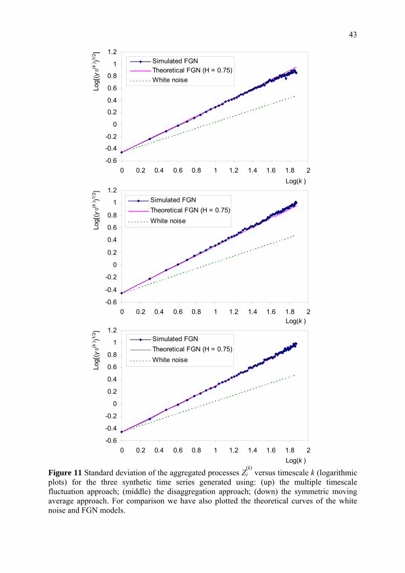
amplitudes at all plotted timescales (1, 5 and 25 years). Figure 11 depicts the standard

deviation of the aggregated processes Z(k)i versus timescale k for the three synthetic time series

generated. For comparison we have also plotted the theoretical curves of the white noise and

FGN models. We observe that all three empirical curves are straight lines on the logarithmic

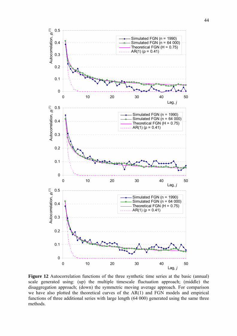
plots with slope 0.75, i.e., equal to the assumed Hurst exponent. Figure 12 depicts the

autocorrelation functions of the three synthetic time series on the basic (annual) scale for lags

up to 50. For comparison we have also plotted the theoretical curves of the AR(1) and FGN

models. We observe that the empirical autocorrelation functions of all three synthetic samples

are close to the theoretical ones of the FGN process with H = 0.75. Some departures are due

to sampling errors as the record length of 1990 values is too small to accurately estimate

autocorrelations for lags as high as 50. To verify this, we also generated three additional

synthetic records with lengths 64 000 values and plotted their autocorrelation functions on

Figure 12, too. We observe that the empirical autocorrelation functions of the latter series are

almost indistinguishable from the theoretical ones of the FGN process. In conclusion, this

demonstration shows that all three methods are good for practical purposes.

7. Conclusions and discussion

A first conclusion of this paper is that the Hurst phenomenon can be formulated and studied in

an easy manner in terms of the variance and autocorrelation of a stochastic process on

multiple timescales, thus avoiding the use of the complicated concept of rescaled range (see

Appendix A1). In addition, the Hurst phenomenon can have a simple and easily

understandable explanation based on the random fluctuation of a hydrologic process upon

22

different timescales. A second conclusion is that the generation of the fractional Gaussian

noise, the process that reproduces the Hurst phenomenon, can be performed by either of three

simple proposed methods that are based on (a) a multiple timescale fluctuation approach, (b) a

disaggregation approach, and (c) a symmetric moving average approach.

Among these three methods, (a) and (b) are very fast as the required computer time on a

common Pentium PC is of the order of tens of milliseconds (for the applications presented in

section 6.4); this becomes of the order of seconds for method (c). Methods (b) and (c) can be

directly extended to generate multivariate series as well (for a general framework of such

adaptations for methods (b) and (c), see Koutsoyiannis, 2001 and 2000, respectively).

Methods (a) and (c) can generate series with skewed distributions. Method (c) is the most

accurate but the other methods are sufficiently accurate and can be directly adapted to further

improve accuracy, as discussed in section 6. In general, all three methods are good for

practical hydrological purposes. Method (a) may be preferable for single variate problems

with symmetric or asymmetric distributions. Method (b) is best for single-variate or

multivariate problems with normal distribution. Finally, method (c) is good for any kind of

problems, single-variate or multivariate with symmetric or asymmetric distributions but it is

slower than the other ones.

Obviously, the FGN process with its singe parameter H is a simplified model of reality.

Therefore, it may be not appropriate for all hydroclimatic series, even though it is much more

consistent with reality in comparison with the AR and ARMA process. A generalised and

comprehensive family of processes, which can include a larger number of parameters and

incorporates both the FGN and the ARMA processes, has been studied by Koutsoyiannis

(2000).

23

Appendix A1: Additional material related to the range concept

In hydrologic texts, the Hurst phenomenon and related topics are analysed in terms of several

storage-related families of random variables (e.g., Yevjevich, 1972; Kottegoda, 1980, p. 184;

Salas, 1993, p. 19.14) like the partial sum

Yn := X1 + X2 + … + Xn (39)

of the stochastic process Xi (i = 1, 2, …), for any integer n; the range

Rn := max(Yi – i µ;1 ≤ i ≤ n) – min(Yi – i µ;1 ≤ i ≤ n) (40)

the adjusted range

R*n := max(Yi – i Yn / n;1 ≤ i ≤ n) – min(Yi – i Yn / n;1 ≤ i ≤ n) (41)

where the true mean µ has been replaced by the sample mean Yn / n; and the rescaled range

R**n = R*

n / Sn (42)

where Sn is the sample standard deviation of X1, X2, …, Xn. We emphasise that Rn, R*n and R**

n

are random variables whose distribution depends on the distribution of Xi, the number n and

the covariance structure of the process X1, X2, …, Xn. The study of the distribution of Rn, R*n ,

and particularly R**n , is a very complicated task. Even their means are difficult to estimate

accurately (Yevjevich, 1972, pp. 148-173). For instance, in the simple case where X1, X2, …,

Xn are independent normal variables with known µ and σ, the mean range is (Yevjevich, 1972,

p. 151)

E[Rn] = σ 2 π ∑

i = 1

n 1 i

(43)

and in the yet simple case where Xi is an AR(1) Gaussian process with known µ and σ, the

mean range is (Yevjevich, 1972, p. 158)

24

E[Rn] = σ 2

π (1 – ρ2) ∑i = 1

n

1 + ρi (1 – ρ) –

2 ρ (1 – ρi)i2 (1 – ρ)2 (44)

(Interestingly, (44) is displayed on the cover of the book by Yevjevich (1972)).

For R*n and R**

n , only approximate relations have been known. For example the mean

adjusted range in the simple case where X1, X2, …, Xn are independent normal variables with

known µ and σ, Yevjevich (1972, p. 152) presents the following equation, obtained by Monte

Carlo simulation using 100 000 independent standard normal numbers:

E[R*n ] ≈ σ ⎝

⎜⎛

⎠⎟⎞π n

2 – π 2 (45)

Generally, it is known that for all ARMA type processes, the rescaled range is asymptotically

E[R**n ] ≈ c n (46)

and for the FGN process

E[R**n ] ≈ c nH (47)

where c is a constant (e.g., Bras and Rodriguez-Iturbe, 1985, p. 221).

Equation (47) has been traditionally used to estimate the Hurst coefficient. However, the

uncertainty implied by (47) is very high. It suffices to say that H can result greater than one

(for example, see Figures 7 and 8 in Vogel et al., 1998), which is not allowed theoretically.

From a conceptual point of view, the range concept corresponds to the mass curve analysis

of a reservoir (plot of cumulated inflows and outflows), a graphical method first developed by

Ripple in 1883 and widely used in reservoir design since then. In this regard, Rn represents the

required storage of a reservoir operating without any spill or other loss and providing a

constant outflow equal to the mean flow. Obviously, this is an oversimplification of a real

reservoir. Therefore, this method needs to be abandoned today and the range concept needs to

be replaced by probability-based design methods.

Because of the complications in definition and conceptualisation of the different range

concepts, the complex relationships of their statistical properties, and the estimation problems,

25

we have avoided using these concepts in the paper. As shown in the paper, the concept of

variance (or standard deviation) on multiple timescales is a much simpler and more accurate

approach, which does not require the range concept at all. However, for the sake of

compatibility with previous studies we have included in this appendix a set of figures related

to the range concept.

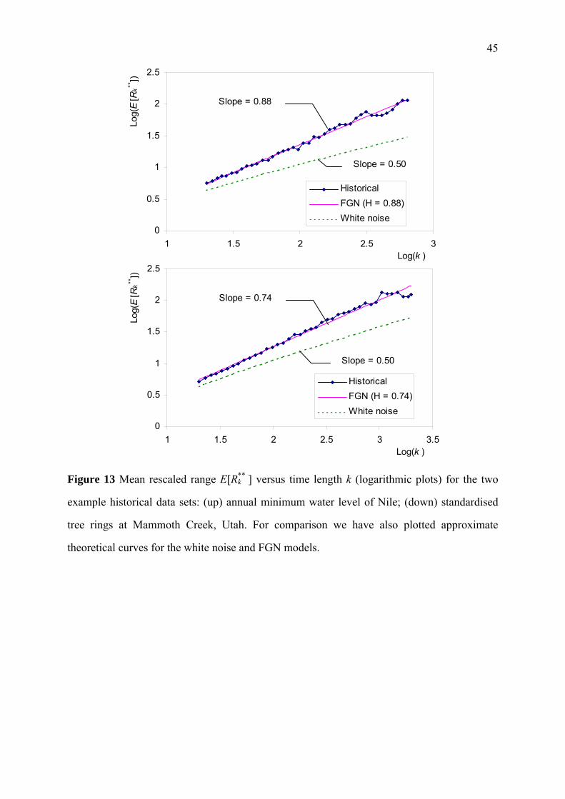
Thus, in Figure 13 we have plotted the mean rescaled range R**n as a function of length n

for the two example historical time series of section 3. We observe that (47) is validated with

H = 0.88 for the Nile time series and H = 0.74 for the Utah time series. These values are close

to the already estimated values (section 3 and Figure 2), H = 0.85 and H = 0.75, respectively.

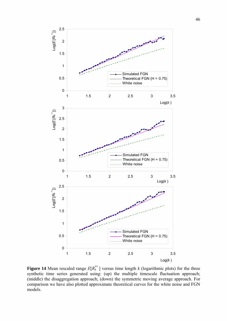
In addition, in Figure 14 we have plotted the mean rescaled range R**n as a function of

length n for the synthetic time series generated in section 6.4. We observe that the slopes of

the empirical curves of R**n versus n on the logarithmic plot are close to the theoretical

expectation H = 0.75.

Appendix A2: Derivation of (18)

We observe that

Z (k j + k)1 = Z

(k j)1 + Z

(k)j + 1 (48)

and consequently

Var[Z (k j + k)1 ] = Var[Z

(k j)1 ] + Var[Z

(k)j + 1] + 2 Cov[Z

(k j)1 , Z

(k)j + 1] (49)

From (17) we get

Var[Z (k j + k)1 ] = ⎝⎜

⎛⎠⎟⎞k j + k

k

H

Var[Z(k)1 ], Var[Z

(k j)1 ] = ⎝⎜

⎛⎠⎟⎞k j

k

H

Var[Z (k) 1 ] (50)

and we conclude that

Cov[Z (k j)1 , Z

(k)j + 1] = (Var[Z

(k) 1 ] / 2) [(j + 1)2H – j2H – 1] (51)

Besides,

26

Z (k j)1 = ∑

i = 1

j Z

(k)i (52)

so that

Cov[Z (k j)1 , Z

(k)j + 1] = Var[Z

(k) 1 ] ∑

i = 1

j ρ

(k)i (53)

and thus

∑i = 1

j ρ

(k)i = (1 / 2) [(j + 1)2H – j2H – 1] (54)

Likewise,

∑i = 1

j – 1 ρ

(k)i = (1 / 2) [j2H – (j – 1)2H – 1] (55)

Subtracting (55) from (54) we get (18).

Acknowledgments. The research leading to this paper was performed within the framework

of the project Modernization of the supervision and management of the water resource system

of Athens, funded by the Water Supply and Sewage Corporation of Athens. The author wishes

to thank the directors of the Corporation and the members of the project committee for the

support of the research. Thanks are also due to I. Nalbantis for his comments.

27

References

Abry, P., P. Gonçalvés and P. Flandrin (1995). Wavelets, spectrum analysis and 1/f processes,

in Wavelets and Statistics, edited by A. Antoniadis and G. Oppenheim, Springer-Verlag,

New York.

Bak, P. (1996). How Nature Works, The Science of Self-Organized Criticality, Copernicus,

Springer-Verlag, New York.

Beran, J. (1994). Statistics for Long-Memory Processes, Volume 61 of Monographs on

Statistics and Applied Probability, Chapman and Hall, New York.

Bhattacharya, R, N., V. K. Gupta and E. Waymire (1983). The Hurst effect under trends, J.

Appl. Prob., 20, 649-662.

Bloomfield, P. (1976). Fourier Analysis of Time Series, Wiley, New York.

Bloomfield, P. (1992). Trends in global temperature, Climate Change, 21, 1-16.

Box, G. E. P., G. M. Jenkins and G. C. Reinsel (1994). Time Series Analysis, Forecasting and

Control, Prentice Hall, Upper Saddle River, New Jersey.

Bras, R.L. and I. Rodriguez-Iturbe (1985). Random Functions in Hydrology, Addison-

Wesley.

Debnath, L. (1995). Integral Transforms and Their Applications, CRC Press, New York.

Ditlevsen, O. D. (1971). Extremes and first passage times, Doctoral dissertation presented to

the Technical University of Denmark, Lyngby, Denmark.

Eltahir, E. A. B. (1996). El Niño and the natural variability in the flow of the Nile River,

Water Resources Research, 32(1) 131-137.

Evans, T. E. (1996). The effects of changes in the world hydrological cycle on availability of

water resources, Chapter 2 in Global Climate Change and Agricultural Production:

Direct and Indirect Effects of Changing Hydrological, Pedological and Plant

Physiological Processes, edited by F. Bazzaz and W. Sombroek, Food and Agriculture

Organization of the United Nations and John Wiley, Chichester.

Graybill, D. A., (1990). IGBP PAGES/World Data Center for Paleoclimatology,

NOAA/NGDC Paleoclimatology Program, Boulder, Colorado, USA.

28

Grygier, J. C. and J. R. Stedinger, (1990). SPIGOT, A synthetic streamflow generation

software package, Technical description, School of Civil and Environmental

Engineering, Cornell University, Ithaca, NY., Version 2.5.

Haan C.T. (1977). Statistical Methods in Hydrology, Iowa State University Press, Ames, 378

pp.

Haslett, J., and A. E. Raftery (1989). Space-time modelling with long-memory dependence:

Assessing Ireland’s wind power resource, Appl. Statist., 38(1), 1-50.

Hosking, J. R. M. (1981). Fractional differencing, Biometrica, 68, 165-176.

Hosking, J. R. M. (1984). Modeling persistence in hydrological time series using fractional

differencing, Water Resources Research, 20(12) 1898-1908.

Hurst, H. E. (1951). Long term storage capacities of reservoirs, Trans. ASCE, 116, 776-808.

Klemes, V. (1974). The Hurst phenomenon: A puzzle?, Water Resour. Res., 10(4) 675-688.

Kottegoda, N. T. (1980). Stochastic Water Resources Technology, Macmillan Press, London.

Koutsoyiannis, D., (2000). A generalized mathematical framework for stochastic simulation

and forecast of hydrologic time series, Water Resources Research, 36(6), 1519-1534.

Koutsoyiannis, D., Coupling stochastic models of different time scales, Water Resources

Research, 37(2), 379-392, 2001.

Lane, W. L. and D. K. Frevert (1990). Applied Stochastic Techniques, User’s Manual, Bureau

of Reclamation, Engineering and Research Center, Denver, Co., Personal Computer

Version.

Mandelbrot, B. B. (1965). Une class de processus stochastiques homothetiques a soi:

Application a la loi climatologique de H. E. Hurst, Compte Rendus Academie Science,

260, 3284-3277.

Mandelbrot, B. B. (1971). A fast fractional Gaussian noise generator, Water Resour. Res.,

7(3), 543-553.

Mandelbrot, B. B. (1977). The Fractal Geometry of Nature, Freeman, New York.

Mandelbrot, B. B., and J. R. Wallis (1969a). Computer experiments with fractional Gaussian

noises, Part 1, Averages and variances, Water Resour. Res., 5(1), 228-241.

29

Mandelbrot, B. B., and J. R. Wallis (1969b). Computer experiments with fractional Gaussian

noises, Part 2, Rescaled ranges and spectra, Water Resour. Res., 5(1), 242-259.

Mandelbrot, B. B., and J. R. Wallis (1969c). Computer experiments with fractional Gaussian

noises, Part 3, Mathematical appendix, Water Resour. Res., 5(1), 260-267.

Mejia, J. M., I. Rodriguez-Iturbe and D. R. Dawdy (1972). Streamflow simulation, 2, The

broken line process as a potential model for hydrologic simulation, Water Resour. Res.,

8(4), 931-941.

Mesa, O. J., and G. Poveda (1993). The Hurst effect: The scale of fluctuation approach, Water

Resour. Res., 29(12), 3995-4002.

Montanari, A., R. Rosso and M. S. Taqqu (1997). Fractionally differenced ARIMA models

applied to hydrologic time series, Water Resour. Res., 33(5), 1035-1044.

National Research Council, (1991). Committee on Opportunities in the Hydrologic Sciences,

Opportunities in the Hydrologic Sciences, National Academy Press, Washington, DC.

Papoulis, A. (1991). Probability, Random Variables, and Stochastic Processes, 3rd ed.,

McGraw-Hill, New York.

Radziejewski, M., and Z. W. Kundzewicz (1997). Fractal analysis of flow of the river Warta,

J. of Hydrol., 200, 280-294.

Salas, J. D. (1993). Analysis and modeling of hydrologic time series, Handbook of

Hydrology, edited by D. Maidment, Chapter 19, pp. 19.1-19.72, McGraw-Hill, New

York.

Salas, J. D., and D. C. Boes (1980). Shifting level modelling of hydrologic time series,

Advances in Water Resources, 3, 59-63.

Salas, J. D., J. W. Delleur, V. Yevjevich, and W. L. Lane (1980). Applied Modeling of

Hydrologic Time Series, Water Resources Publications, Littleton, Colorado.

Saupe, D. (1988). Algorithms for random fractals, Chapter 2 in The Science of Fractal

Images, edited by H.-O. Peitgen and D. Saupe, Springer-Verlag.

Stephenson, D. B., V. Pavan and R. Bojariu (2000). Is the North Atlantic Oscillation a

random walk?, Int. J. Climatol., 20, 1-18.

30

Toussoun, O. (1925). Mémoire sur l’histoire du Nil, in Mémoires a l’Institut d’Egypte, vol.

18, pp. 366-404.

Vanmarke, E. (1983). Random Fields, The MIT Press, Cambridge, Mass.

Vogel, R. M., Y. Tsai and J. F. Limbrunner (1998). The regional persistence and variability of

annual streamflow in the United States, Water Resour. Res., 34(12), 3445-3459.

Yevjevich, V. (1972). Stochastic Processes in Hydrology, Water Resources Publications, Fort

Collins, Colorado.

31

List of Figures

Figure 1 Plots of the two example time series: (up) annual minimum water level of Nile;

(middle) standardised tree rings at Mammoth Creek, Utah. For comparison we have also

plotted (down) a series of white noise with statistics same with those of standardised tree

rings.

Figure 2 Standard deviation of the aggregated processes Z(k)i versus timescale k (logarithmic

plots) for the two example data sets: (up) annual minimum water level of Nile; (down)

standardised tree rings at Mammoth Creek, Utah. For comparison we have also plotted

theoretical curves for the white noise and AR(1) models.

Figure 3 Lag one and lag two autocorrelation coefficients of the aggregated processes Z(k)i

versus timescale k for the two example data sets: (up) annual minimum water level of Nile;

(down) standardised tree rings at Mammoth Creek, Utah. For comparison we have also

plotted the theoretical curves of the AR(1) model.

Figure 4 Autocorrelation functions of the two example time series at the basic (annual) scale:

(up) annual minimum water level of Nile; (down) standardised tree rings at Mammoth Creek,

Utah. For comparison we have also plotted the theoretical curves of the AR(1) model.

Figure 5 Illustrative sketch for multiple timescale random fluctuations of a process that can

explain the Hurst phenomenon: (a) a time series from a Markovian process with constant

mean; (b) the same time series superimposed to a randomly fluctuating mean at a medium

timescale; (c) the same time series further superimposed to a randomly fluctuating mean at a

large timescale.

Figure 6 Plots of the example autocorrelation functions of (a) the Markovian process U with

constant mean; (b) the process U superimposed to a randomly fluctuating mean at a medium

timescale (process V); (c) the process V further superimposed to a randomly fluctuating mean

at a large timescale (process W). The superimposition of fluctuating means increases the lag

32

one autocorrelation (from ρ1 = 0.20 for U to ρ1 = 0.30 and 0.33 for V and W respectively) and

also shifts the autocorrelation function from the AR(1) shape (also plotted in all three panels)

towards the FGN shape (also shown in all three panels).

Figure 7 Approximate autocorrelation functions based on equations (26) and (27) versus the

exact autocorrelation functions of the FGN process for various values of the Hurst exponent

H.

Figure 8 Explanation sketch for the disaggregation approach for generation of a FGN time

series. Grey boxes indicate random variables whose values have been already generated prior

to the current step and arrows indicate the links to those of the generated variables that are

considered in the current generation step.

Figure 9 Approximate autocorrelation functions based on equations (32) and (36) versus the

exact autocorrelation functions of the FGN process for various values of the Hurst exponent H

and the number of weights q.

Figure 10 Plots of the three synthetic time series generated using the statistics of standardised

tree rings at Mammoth Creek, Utah, and implementing: (up) the multiple timescale

fluctuation approach; (middle) the disaggregation approach; (down) the symmetric moving

average approach.

Figure 11 Standard deviation of the aggregated processes Z(k)i versus timescale k (logarithmic

plots) for the three synthetic time series generated using: (up) the multiple timescale

fluctuation approach; (middle) the disaggregation approach; (down) the symmetric moving

average approach. For comparison we have also plotted the theoretical curves of the white

noise and FGN models.

Figure 12 Autocorrelation functions of the three synthetic time series at the basic (annual)

scale generated using: (up) the multiple timescale fluctuation approach; (middle) the

disaggregation approach; (down) the symmetric moving average approach. For comparison

we have also plotted the theoretical curves of the AR(1) and FGN models and empirical

33

functions of three additional series with large length (64 000) generated using the same three

methods.

Figure 13 Mean rescaled range E[R**k ] versus time length k (logarithmic plots) for the two

example historical data sets: (up) annual minimum water level of Nile; (down) standardised

tree rings at Mammoth Creek, Utah. For comparison we have also plotted approximate

theoretical curves for the white noise and FGN models.

Figure 14 Mean rescaled range E[R**k ] versus time length k (logarithmic plots) for the three

synthetic time series generated using: (up) the multiple timescale fluctuation approach;

(middle) the disaggregation approach; (down) the symmetric moving average approach. For

comparison we have also plotted approximate theoretical curves for the white noise and FGN

models.

34

Figures

800

900

1000

1100

1200

1300

1400

1500

600 700 800 900 1000 1100 1200 1300

Year

Nilo

met

er a

nnua

l min

imum

leve

l

Annual value Average, 5 years Average, 25 years

0

0.5

1

1.5

2

2.5

3

0 200 400 600 800 1000 1200 1400 1600 1800 2000Year

Sta

ndar

dise

d tre

e rin

g w

idth Annual value Average, 5 years Average, 25 years

0

0.5

1

1.5

2

2.5

3

0 200 400 600 800 1000 1200 1400 1600 1800 2000

Annual value Average, 5 years Average, 25 years

Figure 1 Plots of the two example time series: (up) annual minimum water level of Nile;

(middle) standardised tree rings at Mammoth Creek, Utah. For comparison we have also

plotted (down) a series of white noise with statistics same with those of standardised tree

rings.

35

1.8

2

2.2

2.4

2.6

2.8

3

3.2

0 0.2 0.4 0.6 0.8 1 1.2 1.4

Log(k )

Log[

(γ0(k

) )1/2 ]

HistoricalAR(1)White noise

Slope = 0.85

Slope = 0.50

Slope = 0.50

-0.6

-0.4

-0.2

0

0.2

0.4

0.6

0.8

1

0 0.2 0.4 0.6 0.8 1 1.2 1.4 1.6 1.8 2

Log(k )

Log[

(γ0(k

) )1/2 ]

HistoricalAR(1)White noise

Slope = 0.75

Slope = 0.50

Slope = 0.50

Figure 2 Standard deviation of the aggregated processes Z(k)i versus timescale k (logarithmic

plots) for the two example data sets: (up) annual minimum water level of Nile; (down)

standardised tree rings at Mammoth Creek, Utah. For comparison we have also plotted

theoretical curves for the white noise and AR(1) models.

36

0

0.1

0.2

0.3

0.4

0.5

0.6

0.7

0.8

0 5 10 15 20 25

Timescale, k

Aut

ocor

rela

tion,

ρ1(k

) , ρ2(k

)

Lag one, HistoricalLag two, HistoricalLag one, Modelled by AR(1)Lag two, Modelled by AR(1)

0

0.1

0.2

0.3

0.4

0.5

0.6

0.7

0.8

0 10 20 30 40 50

Timescale, k

Aut

ocor

rela

tion,

ρ1(k

) , ρ2(k

)

Lag one, HistoricalLag two, HistoricalLag one, Modelled by AR(1)Lag two, Modelled by AR(1)

Figure 3 Lag one and lag two autocorrelation coefficients of the aggregated processes Z(k)i

versus timescale k for the two example data sets: (up) annual minimum water level of Nile;

(down) standardised tree rings at Mammoth Creek, Utah. For comparison we have also

plotted the theoretical curves of the AR(1) model.

37

0

0.1

0.2

0.3

0.4

0.5

0.6

0.7

0 10 20 30 40 50

Lag, j

Aut

ocor

rela

tion,

ρj(1

)

Empirical

Theoretical, AR(1)

0

0.05

0.1

0.15

0.2

0.25

0.3

0.35

0.4

0.45

0.5

0 10 20 30 40 50

Lag, j

Aut

ocor

rela

tion,

ρj(1

) EmpiricalTheoretical, AR(1)

Figure 4 Autocorrelation functions of the two example time series at the basic (annual) scale:

(up) annual minimum water level of Nile; (down) standardised tree rings at Mammoth Creek,

Utah. For comparison we have also plotted the theoretical curves of the AR(1) model.

38

Time, i –>

Val

ue, u

i –

>

Small scale (annual) random fluctuationMean

(a)

Time, i –>

Val

ue, v

i –

>

Small scale (annual) random fluctuationMedium scale random fluctuationMean

(b)

Time, i –>

Val

ue, w

i –

>

Small scale (annual) random fluctuationMedium scale random fluctuationLarge scale random fluctuationMean

(c)

Figure 5 Illustrative sketch for multiple timescale random fluctuations of a process that can

explain the Hurst phenomenon: (a) a time series from a Markovian process with constant

mean; (b) the same time series superimposed to a randomly fluctuating mean at a medium

timescale; (c) the same time series further superimposed to a randomly fluctuating mean at a

large timescale.

39

0

0.1

0.2

0.3

0.4

1 10 100 1000

Aut

ocor

rela

tion,

ρj

Process U (= AR(1))FGN

(a)

0

0.1

0.2

0.3

0.4

1 10 100 1000

Aut

ocor

rela

tion,

ρj

Process VFGNAR(1)

(b)

0

0.1

0.2

0.3

0.4

1 10 100 1000Lag, j

Aut

ocor

rela

tion,

ρj

Process WFGNAR(1)

(c)

Figure 6 Plots of the example autocorrelation functions of (a) the Markovian process U with

constant mean; (b) the process U superimposed to a randomly fluctuating mean at a medium

timescale (process V); (c) the process V further superimposed to a randomly fluctuating mean

at a large timescale (process W). The superimposition of fluctuating means increases the lag

one autocorrelation (from ρ1 = 0.20 for U to ρ1 = 0.30 and 0.33 for V and W respectively) and

also shifts the autocorrelation function from the AR(1) shape (also plotted in all three panels)

towards the FGN shape (also shown in all three panels).

40

0

0.1

0.2

0.3

0.4

0.5

0.6

0.7

0.8

1 10 100 1000Lag, j

Aut

ocor

rela

tion,

ρj

ExactApproximation

H = 0.6

H = 0.7 H = 0.8

H = 0.9

Figure 7 Approximate autocorrelation functions based on equations (26) and (27) versus the

exact autocorrelation functions of the FGN process for various values of the Hurst exponent

H.

Z

(k / 2)2 i + 2

Z(k / 2)1 Z

(k / 2)2

Z(k)1

Z(k / 2)2 i – 3 Z

(k / 2)2 i – 2 Z

(k / 2)2 i – 1 Z

(k / 2)2 i Z

(k / 2)2 i + 1 Z

(k / 2)2 i + 2

Z(k)i – 1 Z

(k)i Z

(k)i + 1

Z(k / 2)2 n / k – 1 Z

(k / 2)2 n / k

Z(k)n / k

Z(n / 2)1 Z

(n / 2)2

Z(n)1

L

L L

L

M M

Current step

Figure 8 Explanation sketch for the disaggregation approach for generation of a FGN time

series. Grey boxes indicate random variables whose values have been already generated prior

to the current step and arrows indicate the links to those of the generated variables that are

considered in the current generation step.

41

0.0001

0.001

0.01

0.1

1

1 10 100 1000 10000Lag, j

Aut

ocor

rela

tion,

ρj

ExactApproximation

H = 0.6, q = 10 000

H = 0.7, q = 10 000

H = 0.8, q = 50 124

H = 0.9, q = 250 000

Figure 9 Approximate autocorrelation functions based on equations (32) and (36) versus the

exact autocorrelation functions of the FGN process for various values of the Hurst exponent H

and the number of weights q.

42

0

0.5

1

1.5

2

2.5

3

0 200 400 600 800 1000 1200 1400 1600 1800 2000Year

Sta

ndar

dise

d tre

e rin

g w

idth Annual value Average, 5 years Average, 25 years

0

0.5

1

1.5

2

2.5

3

0 200 400 600 800 1000 1200 1400 1600 1800 2000Year

Sta

ndar

dise

d tre

e rin

g w

idth Annual value Average, 5 years Average, 25 years

0

0.5

1

1.5

2

2.5

3

0 200 400 600 800 1000 1200 1400 1600 1800 2000Year

Sta

ndar

dise

d tre

e rin

g w

idth Annual value Average, 5 years Average, 25 years

Figure 10 Plots of the three synthetic time series generated using the statistics of standardised

tree rings at Mammoth Creek, Utah, and implementing: (up) the multiple timescale

fluctuation approach; (middle) the disaggregation approach; (down) the symmetric moving

average approach.

43

-0.6

-0.4

-0.2

0

0.2

0.4

0.6

0.8

1

1.2

0 0.2 0.4 0.6 0.8 1 1.2 1.4 1.6 1.8 2Log(k )

Log[

(γ0(k

) )1/2 ]

Simulated FGNTheoretical FGN (H = 0.75)White noise

-0.6

-0.4

-0.2

0

0.2

0.4

0.6

0.8

1

1.2

0 0.2 0.4 0.6 0.8 1 1.2 1.4 1.6 1.8 2Log(k )

Log[

(γ0(k

) )1/2 ]

Simulated FGNTheoretical FGN (H = 0.75)White noise

-0.6

-0.4

-0.2

0

0.2

0.4

0.6

0.8

1

1.2

0 0.2 0.4 0.6 0.8 1 1.2 1.4 1.6 1.8 2Log(k )

Log[

(γ0(k

) )1/2 ]

Simulated FGNTheoretical FGN (H = 0.75)White noise

Figure 11 Standard deviation of the aggregated processes Z

(k)i versus timescale k (logarithmic

plots) for the three synthetic time series generated using: (up) the multiple timescale fluctuation approach; (middle) the disaggregation approach; (down) the symmetric moving average approach. For comparison we have also plotted the theoretical curves of the white noise and FGN models.

44

0

0.1

0.2

0.3

0.4

0.5

0 10 20 30 40 50Lag, j

Aut

ocor

rela

tion,

ρj(1

)

Simulated FGN (n = 1990)Simulated FGN (n = 64 000)Theoretical FGN (H = 0.75)AR(1) (ρ = 0.41)

0

0.1

0.2

0.3

0.4

0.5

0 10 20 30 40 50Lag, j

Aut

ocor

rela

tion,

ρj(1

)

Simulated FGN (n = 1990)Simulated FGN (n = 64 000)Theoretical FGN (H = 0.75)AR(1) (ρ = 0.41)

0

0.1

0.2

0.3

0.4

0.5

0 10 20 30 40 50Lag, j

Aut

ocor

rela

tion,

ρj(1

)

Simulated FGN (n = 1990)Simulated FGN (n = 64 000)Theoretical FGN (H = 0.75)AR(1) (ρ = 0.41)

Figure 12 Autocorrelation functions of the three synthetic time series at the basic (annual) scale generated using: (up) the multiple timescale fluctuation approach; (middle) the disaggregation approach; (down) the symmetric moving average approach. For comparison we have also plotted the theoretical curves of the AR(1) and FGN models and empirical functions of three additional series with large length (64 000) generated using the same three methods.

45

0

0.5

1

1.5

2

2.5

1 1.5 2 2.5 3Log(k )

Log(

E[R

k**

])

HistoricalFGN (H = 0.88)White noise

Slope = 0.50

Slope = 0.88

0

0.5

1

1.5

2

2.5

1 1.5 2 2.5 3 3.5Log(k )

Log(

E[R

k**

])

HistoricalFGN (H = 0.74)White noise

Slope = 0.50

Slope = 0.74

Figure 13 Mean rescaled range E[R**k ] versus time length k (logarithmic plots) for the two

example historical data sets: (up) annual minimum water level of Nile; (down) standardised

tree rings at Mammoth Creek, Utah. For comparison we have also plotted approximate

theoretical curves for the white noise and FGN models.

46

0

0.5

1

1.5

2

2.5

1 1.5 2 2.5 3 3.5

Log(k )

Log(

E[R

k**

])

Simulated FGNTheoretical FGN (H = 0.75)White noise

0

0.5

1

1.5

2

2.5

3

1 1.5 2 2.5 3 3.5Log(k )

Log(

E[R

k**

])

Simulated FGNTheoretical FGN (H = 0.75)White noise

0

0.5

1

1.5

2

2.5

1 1.5 2 2.5 3 3.5

Log(k )

Log(

E[R

k**

])

Simulated FGNTheoretical FGN (H = 0.75)White noise

Figure 14 Mean rescaled range E[R**

k ] versus time length k (logarithmic plots) for the three synthetic time series generated using: (up) the multiple timescale fluctuation approach; (middle) the disaggregation approach; (down) the symmetric moving average approach. For comparison we have also plotted approximate theoretical curves for the white noise and FGN models.