46
April 6, 2005 Massachusetts Institute of Technology Hybrid Estimation for Fault Detection and More Lars Blackmore

April 6, 2005
Massachusetts Institute of Technology
Hybrid Estimationfor Fault Detection and More
Lars Blackmore
2
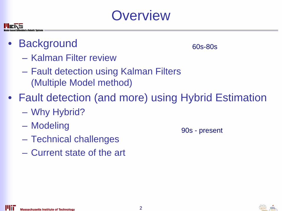
Overview
• Background– Kalman Filter review– Fault detection using Kalman Filters
(Multiple Model method)• Fault detection (and more) using Hybrid Estimation
– Why Hybrid?– Modeling– Technical challenges– Current state of the art
60s-80s
90s - present

3
Fault Detection

4
Kalman Filter Review
• Problem: – Given a continuous dynamic system model:
– And a set of noisy observations:
– Estimate the ‘hidden’ state of the system
)(),()(),,(
11
1
tgttf
ttt
ttt
ωυ
+=+=
++
+
uxyuxx
θVx
Vy

5
Kalman Filter Review
• Solution: Kalman Filters– Calculate belief state about hidden variables
– Approximate as Gaussian
– Predict/update cycle:1. Start with belief state at t-12. Predict belief state at t using system model3. Use measurement at t to adjust the belief state
),|( :1:1 tttp uyx
),ˆ(~),|( :1:1 ttttt Np Pxuyx

6
Kalman Filter Review
• Details– KF equations:
– Linear systems:• State distribution is Gaussian, KF is exact
– Nonlinear systems:• Gaussian assumption is an approximation• Extended Kalman Filter accurate to 1st order• Unscented Kalman Filter accurate to 2nd order
Tttt
Ttttt
ttt f
WQWAPAP
uxx
11
11 ),ˆ(ˆ
−−−
−−−
+=
=Prediction step
( )Tttttt
ttttt g
APHKIP
xyKxx−
−−
−=
−+=
)(
)ˆ(ˆˆMeasurement update step

7
Overview
• Background– Kalman Filter review– Fault detection using Kalman Filters
(Multiple Model method)• Fault detection (and more) using Hybrid Estimation
– Why Hybrid?– Modeling– Technical challenges– Current state of the art
60s-80s
90s - present

8
Multiple Model Fault Detection
• Fault detection:– Is the system operating nominally or is it faulty?
• Assume models known for both cases– Which model most likely given observations and inputs?
• How can we use Kalman Filters here?

9
Multiple Model Fault Detection
• KF predicts distribution of observation given inputs at each time step
• KF ‘innovation’ is discrepancy between expectation and actual observation
• Can use this to determine agreement between model and observations
innovation
)ˆ( −tg x
ty

10
Multiple Model Fault Detection
• Idea:– Use a Kalman Filter for each model– Small innovations model and observations agree– Large innovations model and observations disagree– So compare innovations from faulty and nominal KF– If innovations smaller for faulty KF, diagnose a fault

11
Multiple Model Fault Detection
• More formally– Let each model be denoted by Hi
(e.g. H0=nominal, H1=faulty)– Assume some belief about each model at time t-1:
– We want posterior probability at time t:
– Use Bayes’ Rule:
– We can calculate
)|()( :1 tii Hptp y=
∑=
−
−
−
−= n
jjtjt
ititi
tpHp
tpHptp
11:1
1:1
)1(),|(
)1(),|()(yy
yy
)|()1( 1:1 −=− tii Hptp y
),|( 1:1 −tit Hp yy

12
Multiple Model Fault Detection
• We can calculate– using the Kalman Filter innovation
• So by tracking n Kalman Filters we can calculate the probability of each model given the observations
– Problem solved?
),|( 1:1 −tit Hp yy
ttTteCHp ttit
iViyy 2
1
:1 ),|(−
=Innovation at time t
KFn
…
KF2
KF1observations innovations P(model i)
Probability
calculation

13
Multiple Model Fault Detection
Simulation of‘faulty’ model
Simulation of‘nominal’ model

14
Multiple Model Fault Detection
Time(s)
Simulation of‘faulty’ model
Ground truth
Simulation of‘nominal’ model
Fault occurs here

15
Multiple Model Fault Detection
• Main problem:– Our model of the failure-prone system is inadequate
• Challenges (rest of the lecture):– Model failure-prone systems– Reason about failure-prone systems
(detect faults and more)

16
Overview
• Background– Kalman Filter review– Fault detection using Kalman Filters
• Fault detection (and more) using Hybrid Estimation– Why Hybrid?– Modeling– Technical challenges– Current state of the art
60s-70s
80s - present

17
Hybrid System Models
• Better model for our system:– Discrete modes and transitions between them
– Continuous dynamics corresponding to each mode
nominal failed
0.001
0
0.999 1
)(),()(),,(
nominal1nominal1
nominalnominal1
tgttf
ttt
ttt
ωυ
+=+=
++
+
uxyuxx
)(),()(),,(
failed1failed1
failedfailed1
tgttf
ttt
ttt
ωυ
+=+=
++
+
uxyuxx

18
Hybrid System Models
• System now has hybrid state x={xc,t xd,t}– Continuous state xc,t– Discrete modes xd,t
• Our model is a Hidden Markov Model:
ut-1
ut
xd,t-1
xd,t
xc,t-1
xc,t
yt-1
yt

19
Hybrid System Models
• Hybrid models not just for failure detection
• Many systems have both discrete and continuous state even in normal operation:– Hardware/software controlling physical system
• e.g. Mars rover, robot manipulator
– Systems with valves, switches, doors• Lunar habitat

20
Hybrid System Models
• Even better model:– Model each component as Probabilistic Hybrid Automaton
• Main difference: guards on discrete transitions– Transition probability conditioned on
component inputs and component continuous state• Example:
– More likely to fail if temperature over safe threshold
actuatorinputs outputs
ok failed
g1
g2
0.0010.999
0.90.1
1
21
Hybrid System Models
• ‘Compose’ PHA components to form overall system
• With m modes per PHA, composed PHA has O(mn) modes overall
uc1
ud1
ud2
yc2
yc1
PHA1 PHA2
wc1
PHA3
n components

22
Reasoning about Hybrid System Models
• Now we have trajectories of discrete modes– Example of a possible mode trajectory of the system:
• Known system dynamics for each trajectory
ok ok ok ok ok failed failed failed
t=0 t=1 t=2 t=3 t=4 t=5 t=6 t=7
Time(s)

23
Hybrid Estimation
• Problem:– Estimate the hybrid state of a system
– Given model, observations and system inputs
),|,( :1:1,, tttctdp uyxx

24
Hybrid Estimation
Approach:1. Each time t, consider all possible mode trajectories
2. Calculate the distribution over trajectories and
3. Sum over the trajectories
ok ok
failed
ok
failedfailed
ok
),|,( :1:1,:1, tttctdp uyxx
∑−1:1,
),|,( :1:1,:1,td
tttctdpx
uyxx=),|,( :1:1,, tttctdp uyxx
t=0 t=1 t=2
tc,x

25
Hybrid Estimation
• How to calculate distribution for a trajectory?
• Belief state update:
),|()|()|,( :1:1,,:1:1,:1,:1, ttdtcttdttctd ppp yxxyxyxx =
Probability of trajectorygiven observations Distribution of continuous state given
mode trajectory and observationsgiven by kalman filter
Calculate using belief state update
)()|( :1,:1:1, tdttd bp xyx = )()()( 1:1,, −⋅⋅= tdtdTtO bPP xxy

26
Hybrid Estimation
• Observation function PO
– Track a Kalman Filter for the trajectory
– Use KF innovation (as MM method)
),|( 1:1:1, −= ttdtO pP yxy
td :1,x
ttTteCp tttdt
iViyxy 2
1
1:1:1, ),|(−
− =
27
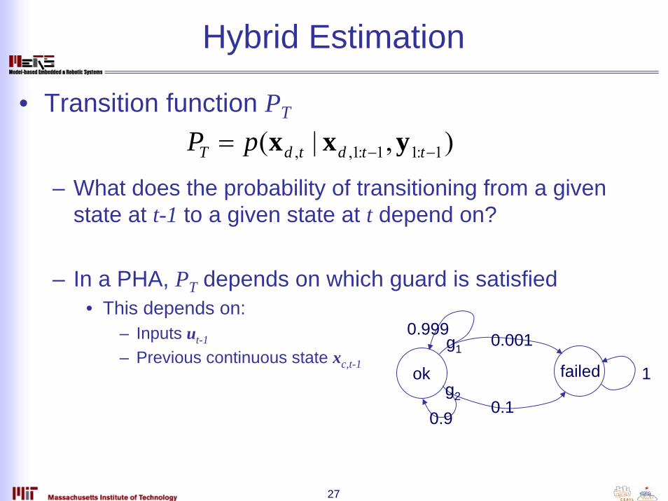
Hybrid Estimation
• Transition function PT
– What does the probability of transitioning from a given state at t-1 to a given state at t depend on?
– In a PHA, PT depends on which guard is satisfied• This depends on:
– Inputs ut-1
– Previous continuous state xc,t-1
),|( 1:11:1,, −−= ttdtdT pP yxx
ok failed
g1
g2
0.0010.999
0.90.1
1

28
Hybrid Estimation
• Probability of guards being satisfied
• P(ok failed)=(0.7)(0.999)+(0.3)(0.9)
ok failed
g1
g2
0.0010.999
0.90.1
1
)( 1, −tcp x
g1 g2
p(g2 satisfied)=0.3
p(g1 satisfied)=0.7
Tth

29
Hybrid Estimation
Approach:1. Each time t, consider all possible mode trajectories
2. Calculate the distribution over trajectories and
3. Sum over the trajectories
• Problems?
ok ok
failed
ok
failedfailed
ok
),|,( :1:1,:1, tttctdp uyxx
∑−1:1,
),|,( :1:1,:1,td
tttctdpx
uyxx=),|,( :1:1,, tttctdp uyxx
t=0 t=1 t=2
tc,x

30
Hybrid Estimation
• Need a KF for each possible mode trajectory– Why is this infeasible?
• Exponential in the number of time steps• Exponential in number of components

31
Approximate Hybrid Estimation
• In practice, we must approximate– Only track some mode trajectories
• Key technical challenge:– Which ones to track?
Information aboutthese trajectories lost

32
Approximate Hybrid Estimation
• Two main successful approaches:1. K-best enumeration
– Greedily pick highest probability trajectories
2. Particle filtering– Stochastic sampling approach

33
K-Best Enumeration
1. Store k trajectories at time t
2. Enumerate the successors at time t+1 in terms of posterior probability
3. Retain the k with the highest posterior probability
4. Discard remainder
• Complexity?
)( :1, tdb x

34
K-Best Enumeration
• Number of successors can be huge– Complexity O(bn) for b successor modes per
component and n components• How to avoid enumeration of all successors?
• Key ideas: – Use conditional independence of components– Frame problem as path search

35
K-Best Enumeration
• Path search through component mode assignments
• Use A* directed search
36
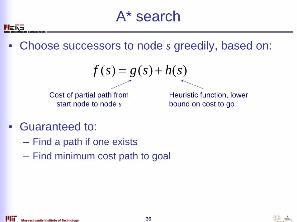
A* search
• Choose successors to node s greedily, based on:
• Guaranteed to:– Find a path if one exists– Find minimum cost path to goal
)()()( shsgsf +=
Cost of partial path fromstart node to node s
Heuristic function, lowerbound on cost to go

37
A* search for K-Best Enumeration
• Cost:– What are we trying to optimise?
• Find maximum probability assignment to allcomponent modes given the observation
– Equivalently we can minimise:
∏=
− ⋅⋅=n
itdTtOtdtd i
PPbb1
,1:1,:1, )()()()( xyxx
)(ln)(ln)(ln)(ln1
,1:1,:1, tO
n
itdTtdtd PPbb
iyxxx −−−=− ∑
=−
Transition probabilityfor component i
38
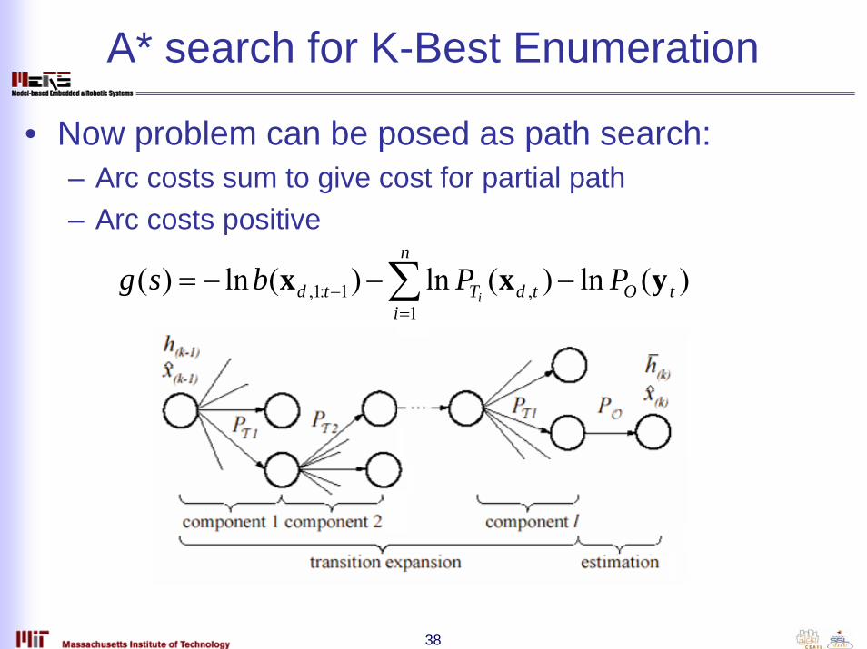
A* search for K-Best Enumeration
• Now problem can be posed as path search:– Arc costs sum to give cost for partial path– Arc costs positive
)(ln)(ln)(ln)(1
,1:1, tO
n
itdTtd PPbsg
iyxx −−−= ∑
=−

39
K-Best Enumeration
• Admissible heuristic?– Need an upper bound on probability of remaining mode
assignments
• PT(ok failed)=p(g1)·0.001+p(g2)·0.1• PT(ok ok)=p(g1)·0.999+p(g2)·0.9
)( 1, −tcp x
g1 g2
p(g2 satisfied)
p(g1 satisfied)
ok failed
g1
g2
0.0010.999
0.90.1
1

40
K-Best Enumeration
• Admissible heuristic:– For each component with mode not yet assigned:– Find the transition with the highest probability– Assume corresponding guard satisfied with probability 1
[ ]∑−=
componentsunassigned
)max(Pln)( Tsh

41
K-Best Enumeration
• Summary– Exponentiality in time:
• Store k best trajectories at each time step
– Exponentiality in number of components:• Efficient successor enumeration using A* search
• Fault detection?– Probability of a given discrete mode easily obtained from
hybrid belief state
– Fault detection problem encompassed in hybrid estimation framework
),|,( :1:1,, tttctdp uyxx
42
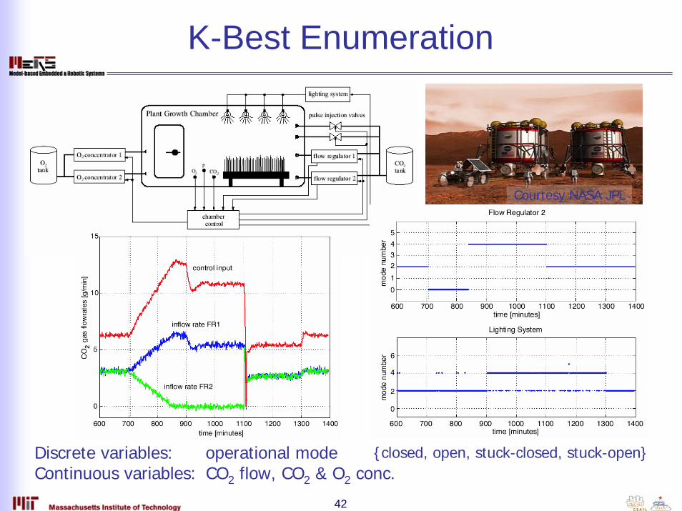
K-Best Enumeration
Courtesy NASA JPL
Discrete variables: operational modeContinuous variables: CO2 flow, CO2 & O2 conc.
{closed, open, stuck-closed, stuck-open}

43
K-Best Enumeration
• Limitations?
• K-best enumeration discards many trajectories– Essentially greedy beam search
• Problem?

44
K-Best Enumeration
• Simple fault example– Consider candidate trajectories A and B
• Which trajectory is most likely?
ok failed
0.001
0
0.999 1
ok ok ok ok ok ok
ok ok ok ok ok failed
t=0 t=0.1 t=0.2 t=0.3 t=0.4 t=0.5
A:
B:
True trajectory
Fault occurs here

45
Recent advances
• Particle filtering
• Smoothing
• Merging
• Risk sensitive estimation
• Mixed greedy/stochastic search

46
Questions?


