energies Article Investigation of Pressure Fluctuation and Pulsating Hydraulic Axial Thrust in Francis Turbines Xing Zhou 1,2 , Changzheng Shi 1, * , Kazuyoshi Miyagawa 2 , Hegao Wu 1, *, Jinhong Yu 1 and Zhu Ma 1 1 State Key Laboratory of Water Resources and Hydropower Engineering Science, Wuhan University, Wuhan 430072, China; [email protected] (X.Z.); [email protected] (J.Y.); [email protected] (Z.M.) 2 Department of Applied Mechanics and Aerospace Engineering, Waseda University, Tokyo 1690072, Japan; [email protected]* Correspondence: [email protected] (C.S.); [email protected] (H.W.) Received: 17 February 2020; Accepted: 2 April 2020; Published: 5 April 2020 Abstract: Under the circumstances of rapid expansion of diverse forms of volatile and intermittent renewable energy sources, hydropower stations have become increasingly indispensable for improving the quality of energy conversion processes. As a consequence, Francis turbines, one of the most popular options, need to operate under off-design conditions, particularly for partial load operation. In this paper, a prototype Francis turbine was used to investigate the pressure fluctuations and hydraulic axial thrust pulsation under four partial load conditions. The analyses of pressure fluctuations in the vaneless space, runner, and draft tube are discussed in detail. The observed precession frequency of the vortex rope is 0.24 times that of the runner rotational frequency, which is able to travel upstream (from the draft tube to the vaneless space). Frequencies of both 24.0 and 15.0 times that of the runner rotational frequency are detected in the recording points of the runner surface, while the main dominant frequency recorded in the vaneless zone is 15.0 times that of the runner rotational frequency. Apart from unsteady pressure fluctuations, the pulsating property of hydraulic axial thrust is discussed in depth. In conclusion, the pulsation of hydraulic axial thrust is derived from the pressure fluctuations of the runner surface and is more complicated than the pressure fluctuations. Keywords: Francis turbine; partial load operation; numerical simulation; pressure fluctuation; hydraulic axial thrust 1. Introduction Presently, renewable energy sources have increasingly contributed to global electricity generation [1]. As a result, the dependence upon fossil fuel is gradually decreasing [2]. In this context, environmental pollution caused by the combustion of fossil fuels is being alleviated accordingly. In the course of developing various renewable and new resources with a long history of exploitation, hydropower holds the largest share and has become one of the most suitable and cost-effective solution for energy supply in both urban and rural areas [2,3]. On a global scale, the hydropower-installed capacity is still growing, and related conservancy projects are expected to prosper, especially in East Asia and the Pacific, South America, and South and Central Asia [1,2]. Hydraulic turbines, one of the critical components of a hydropower plant, are responsible for converting hydro energy into mechanical energy; subsequently, electricity can be generated via a generator. To date, a miscellaneous assortment of hydraulic turbines has been designed to operate reliably and efficiently under different conditions of head and discharge at the actual site [4,5]. Due to desirable advantages, such as a wide operating range and high efficiency, Francis turbines are widely Energies 2020, 13, 1734; doi:10.3390/en13071734 www.mdpi.com/journal/energies
Transcript
energies
Article
Investigation of Pressure Fluctuation and PulsatingHydraulic Axial Thrust in Francis Turbines
Received: 17 February 2020; Accepted: 2 April 2020; Published: 5 April 2020�����������������
Abstract: Under the circumstances of rapid expansion of diverse forms of volatile and intermittentrenewable energy sources, hydropower stations have become increasingly indispensable for improvingthe quality of energy conversion processes. As a consequence, Francis turbines, one of the most popularoptions, need to operate under off-design conditions, particularly for partial load operation. In thispaper, a prototype Francis turbine was used to investigate the pressure fluctuations and hydraulicaxial thrust pulsation under four partial load conditions. The analyses of pressure fluctuations in thevaneless space, runner, and draft tube are discussed in detail. The observed precession frequency ofthe vortex rope is 0.24 times that of the runner rotational frequency, which is able to travel upstream(from the draft tube to the vaneless space). Frequencies of both 24.0 and 15.0 times that of therunner rotational frequency are detected in the recording points of the runner surface, while themain dominant frequency recorded in the vaneless zone is 15.0 times that of the runner rotationalfrequency. Apart from unsteady pressure fluctuations, the pulsating property of hydraulic axialthrust is discussed in depth. In conclusion, the pulsation of hydraulic axial thrust is derived from thepressure fluctuations of the runner surface and is more complicated than the pressure fluctuations.
Presently, renewable energy sources have increasingly contributed to global electricitygeneration [1]. As a result, the dependence upon fossil fuel is gradually decreasing [2]. In this context,environmental pollution caused by the combustion of fossil fuels is being alleviated accordingly.In the course of developing various renewable and new resources with a long history of exploitation,hydropower holds the largest share and has become one of the most suitable and cost-effective solutionfor energy supply in both urban and rural areas [2,3]. On a global scale, the hydropower-installedcapacity is still growing, and related conservancy projects are expected to prosper, especially in EastAsia and the Pacific, South America, and South and Central Asia [1,2].
Hydraulic turbines, one of the critical components of a hydropower plant, are responsible forconverting hydro energy into mechanical energy; subsequently, electricity can be generated via agenerator. To date, a miscellaneous assortment of hydraulic turbines has been designed to operatereliably and efficiently under different conditions of head and discharge at the actual site [4,5]. Due todesirable advantages, such as a wide operating range and high efficiency, Francis turbines are widely
used compared to other types of hydraulic turbines [6,7]. With the advantage being able to regulateoperating conditions for a rather low cost and short time, Francis turbines are able to meet real-timeelectricity demands and, thus, are frequently employed to stabilize power grid operation [6,8,9].However, Francis turbines are generally designed to operate at the best efficiency points (BEPs) and,theoretically, the flow leaving the runner is almost axial, with little swirl entering the draft tube.Francis turbines are inevitably operated from a partial to full load for the sake of accommodatingthe real-time demand of end-users, which is likely to bring about unfavorable issues that underminehydraulic stability, including Karman vortex at the trailing edge of guide vanes, blade channel vortices,and helical vortex rope in the draft tube [10,11]. In addition, being one of the crucial factors in hydraulicstability, hydraulic axial thrust represents severe fluctuations and poses a great threat to the bearingand powerhouse structure under off-design conditions.
Hydraulic axial thrust is mainly comprised of the axial force on the surface of runner bladesand the inner and outer surface of the crown and band. Numerous studies can be found regardingtheoretical calculation of the hydraulic axial thrust for the design of the thrust bearing and powerhousestructure [12]. In these studies, a constant was determined for specific operating points, and this hassatisfied the design criteria. However, the theoretical equations fail to take fluctuation of hydraulic axialthrust into account, which can no longer be ignored given the increasing attention toward the vibrationproblem of Francis turbines. To achieve this, both laboratory measurements and computational fluiddynamics (CFD) can be used to obtain the evolution of hydraulic axial thrust over time. The latteris favored by researchers for its benefits of robustness, convenience, and capturing of detailed fluidinformation. To date, CFD methodology has been adopted by researchers and engineers not only toelaborate such complex dynamic fluid flow effects, but also to carry out the optimization of turbinecomponents during design or rehabilitation [13,14].
Over the last several decades, both experiments and numerical simulations have been performed toinvestigate flow instabilities as well as the induced pressure fluctuations inside Francis turbines [15,16].Arpe et al. [17] presented a detailed experimental study about the unstable pressure field that developedunder low-discharge operating conditions within the elbow-type draft tube of a high specific speedFrancis turbine. They found that pressure fluctuations resulted from the vortex precession within therange of 0.2–0.4 fn (runner rotational frequency), which were generated only in the conical part ofthe draft tube and then disappeared in the straight diffuser. Müller et al. [18] showed the high-speedvisualization of the runner blade channel flow pattern during one pressure oscillating period andconcluded that the critical cavitation evolution on the runner blades modified their hydrodynamicperformance to some degree, so as to result in a reduction in the momentum transferred from flowto the turbine shaft. Frunzverde et al. [19] illustrated a case of runner failure in a low head Francisturbine, where a crack was discovered at the junction between the blade leading edge and the crown.Their discussion revealed that both the rotor stator interaction (RSI) and the vortex rope were capableof giving rise to dynamic stresses in the runner blades. Trivedi and Cervantes [20] reviewed the studiesconducted on RSI within hydraulic turbines and pointed out that the frequencies in the stationary androtating domains were computed using fr = n·Zgv and fs = n·Zb, respectively. In the two equations,n referred to the runner speed in revolutions per second, and Zgv and Zb were the number of guidevanes and rotating blades, respectively. Xia et al. [21] investigated the pressure fluctuations and runnerloads on a Francis pump-turbine runner during the runaway process, and found that the variationof discharge was the main reason for the intense fluctuation in hydraulic thrust during this process.However, limited studies are associated with the pulsating property of hydraulic axial thrust underthe impact of multiple hydraulic excitation forces. Being one of the crucial factors in hydraulic stability,hydraulic axial thrust is the resultant force in the axial direction of the turbine runner exerted by theflow in the turbine passage, which is then transmitted to the load-bearing frame base of the powerhousevia thrust bearing, and consequently, poses a threat to the bearing and the powerhouse. As Francisturbines are more liable to operating under off-design conditions than before, it is imperative to have adeeper understanding of hydraulic thrust for the safe and stable operation of hydropower stations.
Energies 2020, 13, 1734 3 of 16
To bridge the gap that exists in the available state-of-the-art studies on hydraulic axial thrust,the aim of this paper was to numerically analyze the pulsating property of hydraulic axial thrust underthe impact of multiple hydraulic excitation forces. Given that the size of the labyrinth seal gap is muchsmaller than that of the main turbine passage, it is hard to take the labyrinth seal into considerationin the whole turbine model simulation. In addition, a small variation in seal clearance would have asignificant influence over the thrust value and, therefore, only axial force on the surface of the runnerblades and inner surface of the crown and band were investigated in this paper. After conducting theperformance evaluation, the Francis turbine operated at four different guide vane openings (GVOs)was explored in order to fully study the pressure fluctuations in the draft tube, runner, and vanelessspace, as well as to clarify the fluctuation mechanism of hydraulic axial thrust.
2. Numerical Model
2.1. Computational Domain
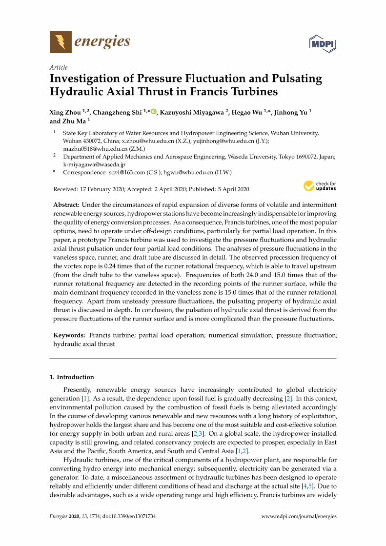
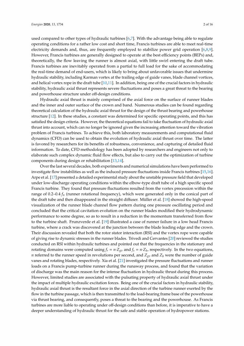
The Francis turbine investigated in this study is a prototype that operates in a hydropower plantin China. Its design head is 116.0 m, the rated volume flow rate is 87.72 m3/s, the rated power output is90 MW, and the designed rotational speed is 250 r/min. Figure 1a shows the whole turbine geometry inthe following simulations. Figure 1b–e presents the discretization of a spiral case, a tandem cascade,a runner blade, and a draft tube, respectively. The computational domain includes five subdomains,i.e., a spiral case, a region with 24 stay vanes, a region with 24 guide vanes, a region with 15 runnerblades, and a draft tube. Two kinds of mesh were created for these five domains via TurboGrid14.5 and ANSYS ICEM 14.5 to produce high-quality grids. The spiral case, stay and guide vanes,and draft tube were discretized using hexahedral grids, while tetrahedral grids were generated in therunner. As for the number of grids, eight different sizes of grids with element numbers varying from0.98 × 106 to 8.32 × 10⁶ were created at 18 deg guide vane opening to conduct the mesh sensitivityanalysis (see Figure 2). After confirmation of the variation of average volume flow rate and runnertorque with the grid number and taking into account the trade-off between the required computationalresources and the calculation accuracy, a total number of 4.12 × 10⁶ grids was used for the subsequentinvestigation (see Table 1).
Energies 2020, 13, x FOR PEER REVIEW 3 of 16
To bridge the gap that exists in the available state‐of‐the‐art studies on hydraulic axial thrust,
the aim of this paper was to numerically analyze the pulsating property of hydraulic axial thrust
under the impact of multiple hydraulic excitation forces. Given that the size of the labyrinth seal gap
is much smaller than that of the main turbine passage, it is hard to take the labyrinth seal into
consideration in the whole turbine model simulation. In addition, a small variation in seal clearance
would have a significant influence over the thrust value and, therefore, only axial force on the surface
of the runner blades and inner surface of the crown and band were investigated in this paper. After
conducting the performance evaluation, the Francis turbine operated at four different guide vane
openings (GVOs) was explored in order to fully study the pressure fluctuations in the draft tube,
runner, and vaneless space, as well as to clarify the fluctuation mechanism of hydraulic axial thrust.
2. Numerical Model
2.1. Computational Domain
The Francis turbine investigated in this study is a prototype that operates in a hydropower plant
in China. Its design head is 116.0 m, the rated volume flow rate is 87.72 m3/s, the rated power output
is 90 MW, and the designed rotational speed is 250 r/min. Figure 1a shows the whole turbine
geometry in the following simulations. Figure 1b–e presents the discretization of a spiral case, a
tandem cascade, a runner blade, and a draft tube, respectively. The computational domain includes
five subdomains, i.e., a spiral case, a region with 24 stay vanes, a region with 24 guide vanes, a region
with 15 runner blades, and a draft tube. Two kinds of mesh were created for these five domains via
TurboGrid 14.5 and ANSYS ICEM 14.5 to produce high‐quality grids. The spiral case, stay and guide
vanes, and draft tube were discretized using hexahedral grids, while tetrahedral grids were
generated in the runner. As for the number of grids, eight different sizes of grids with element
numbers varying from 0.98 × 10⁶ to 8.32 × 10⁶ were created at 18 deg guide vane opening to conduct
the mesh sensitivity analysis (see Figure 2). After confirmation of the variation of average volume
flow rate and runner torque with the grid number and taking into account the trade‐off between the
required computational resources and the calculation accuracy, a total number of 4.12 × 10⁶ grids was
used for the subsequent investigation (see Table 1).
(b) (c)
(a) (d) (e)
Figure 1. Geometry and mesh in the current simulation for (a) total, (b) spiral case, (c) tandem cascade,
(d) blade, and (e) draft tube. Figure 1. Geometry and mesh in the current simulation for (a) total, (b) spiral case, (c) tandem cascade,(d) blade, and (e) draft tube.
Energies 2020, 13, 1734 4 of 16Energies 2020, 13, x FOR PEER REVIEW 4 of 16
Figure 2. Grid number sensitivity analysis (18 deg GVO).
Table 1. Number of grids (million).
Component Spiral Case Stay Vane Guide Vane Runner Draft Tube Total
Elements 0.09 0.84 1.20 1.48 0.51 4.12
Nodes 0.06 0.77 1.10 0.26 0.49 2.68
2.2. Turbulence Model, Numerical Schemes and Boundary Conditions
FLUENT 14.5 was employed to conduct CFD simulations, and main setting parameters
employed are displayed in Table 2. Most of the simulation processes and setup were consistent with
the author’s previous paper [8]. However, a smaller time step of 0.0005 s corresponding to 0.75 degree
of runner rotation was chosen in this paper to better capture the high‐frequency dynamic effects
inside the whole flow passage [22,23]; the total time of calculation was set to 10 s (about 40 runner
revolutions). The flow rates of four different partial load conditions were achieved by changing the
guide vane opening while ensuring the same inlet and outlet pressure to maintain the water head
design. Due to the inconsistency of grids between adjacent subdomains, four interfaces were created
for transferring computational information, namely between the spiral case and the stay vane,
between the stay vane and the guide vane, between the guide vane and the runner, and between the
runner and the draft tube.
Table 2. Numerical setting parameters.
Turbulence
Model
Boundary Conditions Rotation
Speed of the
Runner
Discretization Scheme Time
Step Pressure
Inlet
Pressure
Outlet
Diffusion
Term
Convective
Term
RNG k– 1.18 MPa 0.04 MPa 250 rpm
second‐order
central
difference
Second‐order
upwind 0.0005 s
2.3. Recording Points and Sections
Fourteen points located in the vaneless space, the runner, and the draft tube (see red crosses in
Figure 3) were selected to record the time‐resolved pressure. Three monitoring points of R1p, R2p, and
R3p were located on the pressure side of one blade from near the runner inlet to near the runner outlet,
while three others, R1n, R2n, and R3n, were positioned in the corresponding locations on the suction
side of the same blade. Four monitoring points, defined as H1 and H2, and S1 and S2, were located on
the runner hub and shroud, respectively. For the recording points belonging to stationary walls, they
were created by specifying each individual Cartesian coordinate. Meanwhile, for the monitoring
points attached to the rotating walls (such as runner blades), there were two steps: firstly, an
intersecting line between the blade vanes and a cylindrical surface was drawn; then, the
corresponding points can be created by seeking the intersection of this intersecting line with a z‐axis
Figure 2. Grid number sensitivity analysis (18 deg GVO).
Table 1. Number of grids (million).
Component Spiral Case Stay Vane Guide Vane Runner Draft Tube Total
2.2. Turbulence Model, Numerical Schemes and Boundary Conditions
FLUENT 14.5 was employed to conduct CFD simulations, and main setting parameters employedare displayed in Table 2. Most of the simulation processes and setup were consistent with the author’sprevious paper [8]. However, a smaller time step of 0.0005 s corresponding to 0.75 degree of runnerrotation was chosen in this paper to better capture the high-frequency dynamic effects inside the wholeflow passage [22,23]; the total time of calculation was set to 10 s (about 40 runner revolutions). The flowrates of four different partial load conditions were achieved by changing the guide vane opening whileensuring the same inlet and outlet pressure to maintain the water head design. Due to the inconsistencyof grids between adjacent subdomains, four interfaces were created for transferring computationalinformation, namely between the spiral case and the stay vane, between the stay vane and the guidevane, between the guide vane and the runner, and between the runner and the draft tube.
Table 2. Numerical setting parameters.
TurbulenceModel
Boundary Conditions Rotation Speedof the Runner
Discretization Scheme TimeStepPressure Inlet Pressure Outlet Diffusion Term Convective Term
RNG k–ε 1.18 MPa 0.04 MPa 250 rpmsecond-order
centraldifference
Second-orderupwind 0.0005 s
2.3. Recording Points and Sections
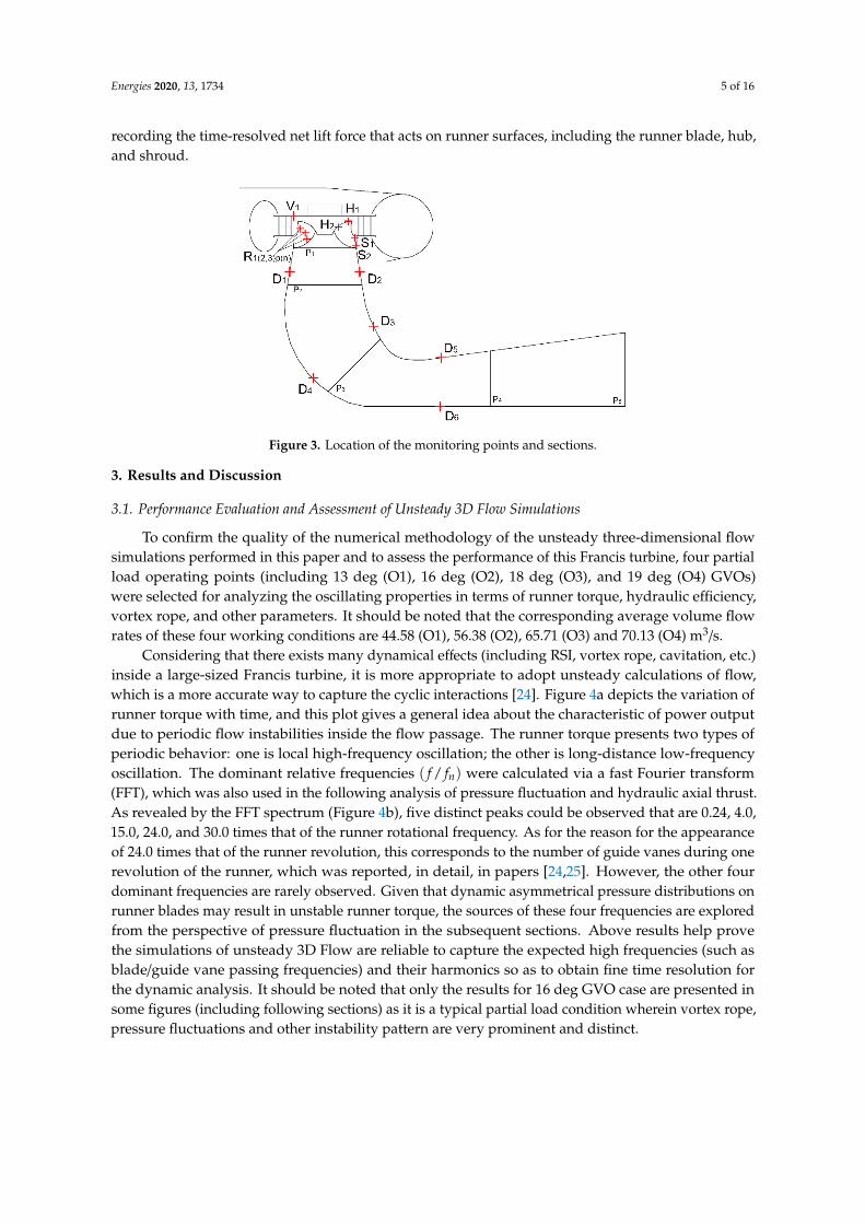
Fourteen points located in the vaneless space, the runner, and the draft tube (see red crosses inFigure 3) were selected to record the time-resolved pressure. Three monitoring points of R1p, R2p,and R3p were located on the pressure side of one blade from near the runner inlet to near the runner outlet,while three others, R1n, R2n, and R3n, were positioned in the corresponding locations on the suction sideof the same blade. Four monitoring points, defined as H1 and H2, and S1 and S2, were located on therunner hub and shroud, respectively. For the recording points belonging to stationary walls, they werecreated by specifying each individual Cartesian coordinate. Meanwhile, for the monitoring pointsattached to the rotating walls (such as runner blades), there were two steps: firstly, an intersectingline between the blade vanes and a cylindrical surface was drawn; then, the corresponding pointscan be created by seeking the intersection of this intersecting line with a z-axis plane. Five sections,ascending from P1 to P5 (indicated in Figure 3), were chosen to analyze the pressure distributionin the draft tube passage. To investigate hydraulic axial thrust, the monitoring was conducted by
Energies 2020, 13, 1734 5 of 16
recording the time-resolved net lift force that acts on runner surfaces, including the runner blade, hub,and shroud.
Energies 2020, 13, x FOR PEER REVIEW 5 of 16
plane. Five sections, ascending from P1 to P5 (indicated in Figure 3), were chosen to analyze the
pressure distribution in the draft tube passage. To investigate hydraulic axial thrust, the monitoring
was conducted by recording the time‐resolved net lift force that acts on runner surfaces, including
the runner blade, hub, and shroud.
Figure 3. Location of the monitoring points and sections.
3. Results and Discussion
3.1. Performance Evaluation and Assessment of Unsteady 3D Flow Simulations
To confirm the quality of the numerical methodology of the unsteady three‐dimensional flow
simulations performed in this paper and to assess the performance of this Francis turbine, four partial
load operating points (including 13 deg (O1), 16 deg (O2), 18 deg (O3), and 19 deg (O4) GVOs) were
selected for analyzing the oscillating properties in terms of runner torque, hydraulic efficiency, vortex
rope, and other parameters. It should be noted that the corresponding average volume flow rates of
these four working conditions are 44.58 (O1), 56.38 (O2), 65.71 (O3) and 70.13 (O4) m3/s.
Considering that there exists many dynamical effects (including RSI, vortex rope, cavitation,
etc.) inside a large‐sized Francis turbine, it is more appropriate to adopt unsteady calculations of flow,
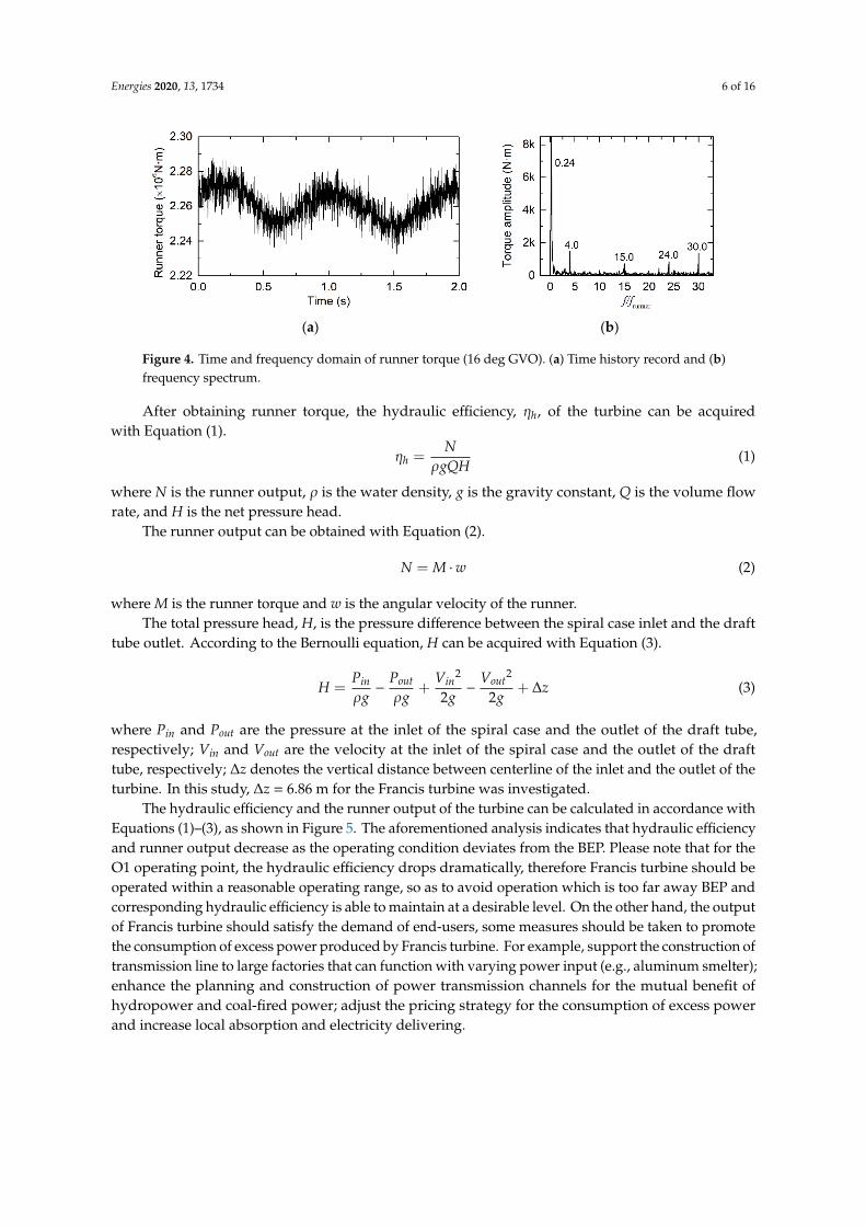
which is a more accurate way to capture the cyclic interactions [24]. Figure 4a depicts the variation of
runner torque with time, and this plot gives a general idea about the characteristic of power output
due to periodic flow instabilities inside the flow passage. The runner torque presents two types of
periodic behavior: one is local high‐frequency oscillation; the other is long‐distance low‐frequency
oscillation. The dominant relative frequencies 𝑓 𝑓⁄ were calculated via a fast Fourier transform
(FFT), which was also used in the following analysis of pressure fluctuation and hydraulic axial
thrust. As revealed by the FFT spectrum (Figure 4b), five distinct peaks could be observed that are
0.24, 4.0, 15.0, 24.0, and 30.0 times that of the runner rotational frequency. As for the reason for the
appearance of 24.0 times that of the runner revolution, this corresponds to the number of guide vanes
during one revolution of the runner, which was reported, in detail, in papers [24,25]. However, the
other four dominant frequencies are rarely observed. Given that dynamic asymmetrical pressure
distributions on runner blades may result in unstable runner torque, the sources of these four
frequencies are explored from the perspective of pressure fluctuation in the subsequent sections.
Above results help prove the simulations of unsteady 3D Flow are reliable to capture the expected
high frequencies (such as blade/guide vane passing frequencies) and their harmonics so as to obtain
fine time resolution for the dynamic analysis. It should be noted that only the results for 16 deg GVO
case are presented in some figures (including following sections) as it is a typical partial load
condition wherein vortex rope, pressure fluctuations and other instability pattern are very prominent
and distinct.
Figure 3. Location of the monitoring points and sections.
3. Results and Discussion
3.1. Performance Evaluation and Assessment of Unsteady 3D Flow Simulations
To confirm the quality of the numerical methodology of the unsteady three-dimensional flowsimulations performed in this paper and to assess the performance of this Francis turbine, four partialload operating points (including 13 deg (O1), 16 deg (O2), 18 deg (O3), and 19 deg (O4) GVOs)were selected for analyzing the oscillating properties in terms of runner torque, hydraulic efficiency,vortex rope, and other parameters. It should be noted that the corresponding average volume flowrates of these four working conditions are 44.58 (O1), 56.38 (O2), 65.71 (O3) and 70.13 (O4) m3/s.
Considering that there exists many dynamical effects (including RSI, vortex rope, cavitation, etc.)inside a large-sized Francis turbine, it is more appropriate to adopt unsteady calculations of flow,which is a more accurate way to capture the cyclic interactions [24]. Figure 4a depicts the variation ofrunner torque with time, and this plot gives a general idea about the characteristic of power outputdue to periodic flow instabilities inside the flow passage. The runner torque presents two types ofperiodic behavior: one is local high-frequency oscillation; the other is long-distance low-frequencyoscillation. The dominant relative frequencies ( f / fn) were calculated via a fast Fourier transform(FFT), which was also used in the following analysis of pressure fluctuation and hydraulic axial thrust.As revealed by the FFT spectrum (Figure 4b), five distinct peaks could be observed that are 0.24, 4.0,15.0, 24.0, and 30.0 times that of the runner rotational frequency. As for the reason for the appearanceof 24.0 times that of the runner revolution, this corresponds to the number of guide vanes during onerevolution of the runner, which was reported, in detail, in papers [24,25]. However, the other fourdominant frequencies are rarely observed. Given that dynamic asymmetrical pressure distributions onrunner blades may result in unstable runner torque, the sources of these four frequencies are exploredfrom the perspective of pressure fluctuation in the subsequent sections. Above results help provethe simulations of unsteady 3D Flow are reliable to capture the expected high frequencies (such asblade/guide vane passing frequencies) and their harmonics so as to obtain fine time resolution forthe dynamic analysis. It should be noted that only the results for 16 deg GVO case are presented insome figures (including following sections) as it is a typical partial load condition wherein vortex rope,pressure fluctuations and other instability pattern are very prominent and distinct.
Energies 2020, 13, 1734 6 of 16Energies 2020, 13, x FOR PEER REVIEW 6 of 16
(a) (b)
Figure 4. Time and frequency domain of runner torque (16 deg GVO). (a) Time history record and (b)
frequency spectrum.
After obtaining runner torque, the hydraulic efficiency, h , of the turbine can be acquired with
Equation (1).
=h
N
gQH
(1)
where N is the runner output, is the water density, g is the gravity constant, Q is the volume
flow rate, and H is the net pressure head. The runner output can be obtained with Equation (2).
=N M w (2)
where M is the runner torque and w is the angular velocity of the runner.
The total pressure head, H, is the pressure difference between the spiral case inlet and the draft
tube outlet. According to the Bernoulli equation, H can be acquired with Equation (3).
2 2
=2 2
in out in outP P V VH z
g g g g
(3)
where inP and outP are the pressure at the inlet of the spiral case and the outlet of the draft tube,
respectively; inV and outV are the velocity at the inlet of the spiral case and the outlet of the draft
tube, respectively; ∆z denotes the vertical distance between centerline of the inlet and the outlet of
the turbine. In this study, ∆z = 6.86 m for the Francis turbine was investigated.
The hydraulic efficiency and the runner output of the turbine can be calculated in accordance
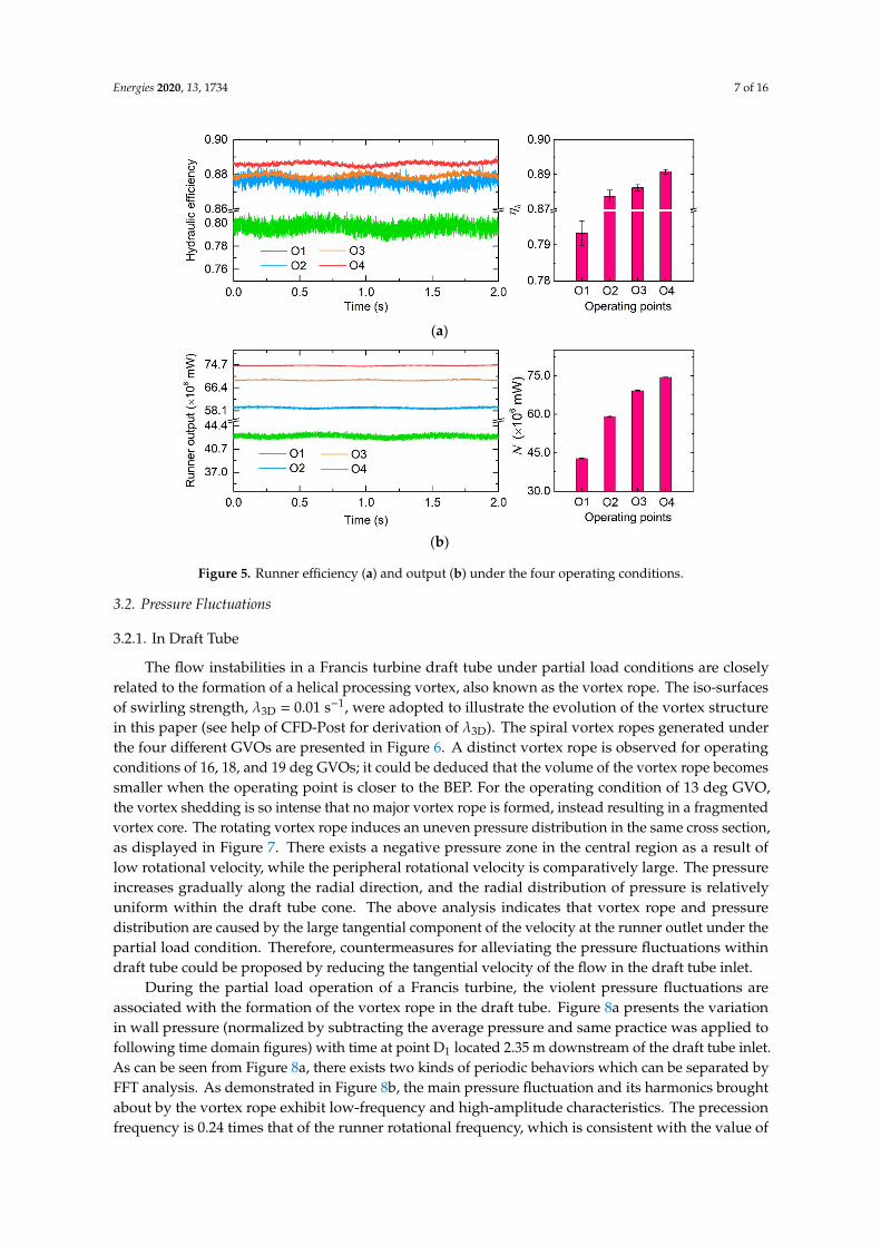
with Equations (1)–(3), as shown in Figure 5. The aforementioned analysis indicates that hydraulic
efficiency and runner output decrease as the operating condition deviates from the BEP. Please note
that for the O1 operating point, the hydraulic efficiency drops dramatically, therefore Francis turbine
should be operated within a reasonable operating range, so as to avoid operation which is too far
away BEP and corresponding hydraulic efficiency is able to maintain at a desirable level. On the other
hand, the output of Francis turbine should satisfy the demand of end‐users, some measures should
be taken to promote the consumption of excess power produced by Francis turbine. For example,
support the construction of transmission line to large factories that can function with varying power
input (e.g., aluminum smelter); enhance the planning and construction of power transmission
channels for the mutual benefit of hydropower and coal‐fired power; adjust the pricing strategy for
the consumption of excess power and increase local absorption and electricity delivering.
Figure 4. Time and frequency domain of runner torque (16 deg GVO). (a) Time history record and (b)frequency spectrum.
After obtaining runner torque, the hydraulic efficiency, ηh, of the turbine can be acquiredwith Equation (1).
ηh =N
ρgQH(1)
where N is the runner output, ρ is the water density, g is the gravity constant, Q is the volume flowrate, and H is the net pressure head.
The runner output can be obtained with Equation (2).
N = M ·w (2)
where M is the runner torque and w is the angular velocity of the runner.The total pressure head, H, is the pressure difference between the spiral case inlet and the draft
tube outlet. According to the Bernoulli equation, H can be acquired with Equation (3).
H =Pinρg−
Pout
ρg+
Vin2
2g−
Vout2
2g+ ∆z (3)
where Pin and Pout are the pressure at the inlet of the spiral case and the outlet of the draft tube,respectively; Vin and Vout are the velocity at the inlet of the spiral case and the outlet of the drafttube, respectively; ∆z denotes the vertical distance between centerline of the inlet and the outlet of theturbine. In this study, ∆z = 6.86 m for the Francis turbine was investigated.
The hydraulic efficiency and the runner output of the turbine can be calculated in accordance withEquations (1)–(3), as shown in Figure 5. The aforementioned analysis indicates that hydraulic efficiencyand runner output decrease as the operating condition deviates from the BEP. Please note that for theO1 operating point, the hydraulic efficiency drops dramatically, therefore Francis turbine should beoperated within a reasonable operating range, so as to avoid operation which is too far away BEP andcorresponding hydraulic efficiency is able to maintain at a desirable level. On the other hand, the outputof Francis turbine should satisfy the demand of end-users, some measures should be taken to promotethe consumption of excess power produced by Francis turbine. For example, support the construction oftransmission line to large factories that can function with varying power input (e.g., aluminum smelter);enhance the planning and construction of power transmission channels for the mutual benefit ofhydropower and coal-fired power; adjust the pricing strategy for the consumption of excess powerand increase local absorption and electricity delivering.
Energies 2020, 13, 1734 7 of 16Energies 2020, 13, x FOR PEER REVIEW 7 of 16
(a)
(b)
Figure 5. Runner efficiency (a) and output (b) under the four operating conditions.
3.2. Pressure Fluctuations
3.2.1. In Draft Tube
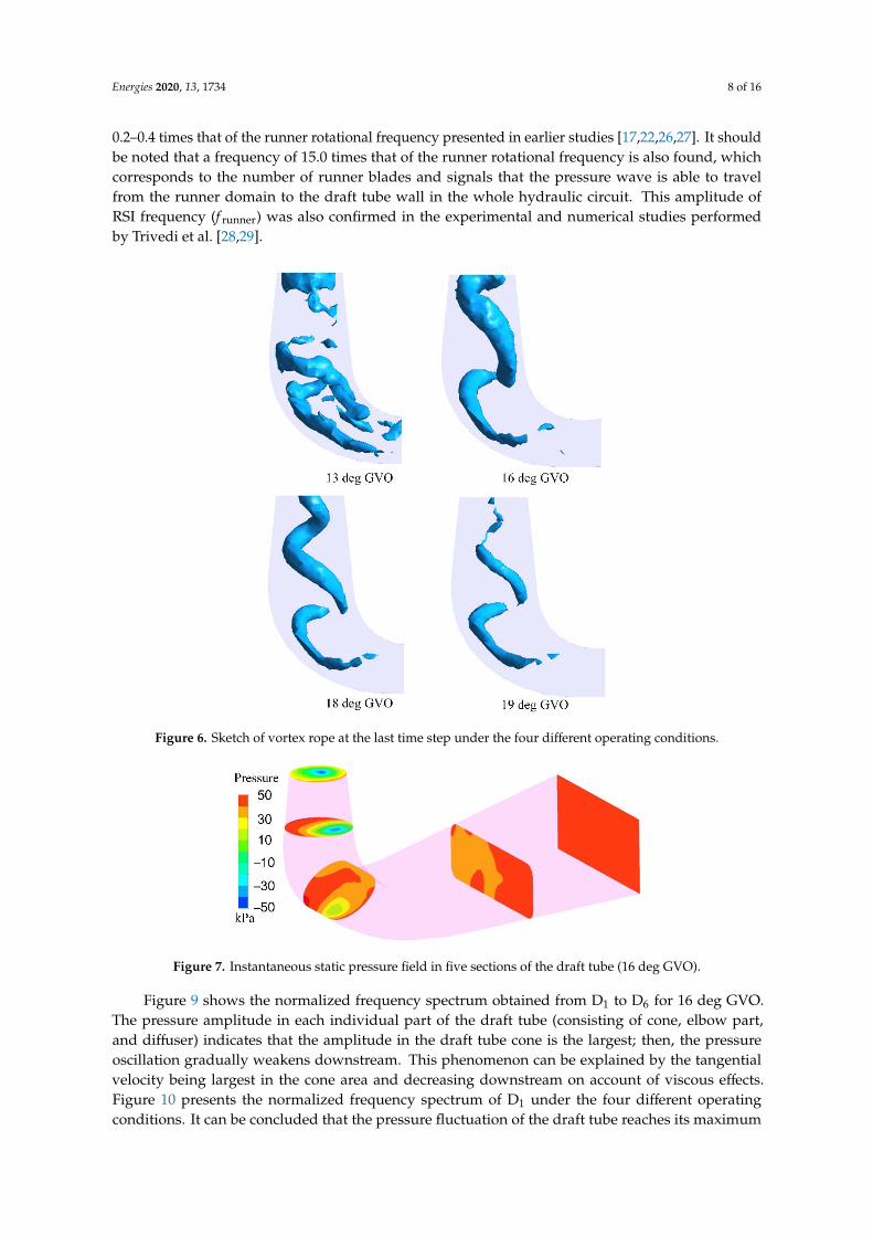
The flow instabilities in a Francis turbine draft tube under partial load conditions are closely
related to the formation of a helical processing vortex, also known as the vortex rope. The iso‐surfaces
of swirling strength, λ3D = 0.01 s−1, were adopted to illustrate the evolution of the vortex structure in
this paper (see help of CFD‐Post for derivation of λ3D). The spiral vortex ropes generated under the
four different GVOs are presented in Figure 6. A distinct vortex rope is observed for operating
conditions of 16, 18, and 19 deg GVOs; it could be deduced that the volume of the vortex rope
becomes smaller when the operating point is closer to the BEP. For the operating condition of 13 deg
GVO, the vortex shedding is so intense that no major vortex rope is formed, instead resulting in a
fragmented vortex core. The rotating vortex rope induces an uneven pressure distribution in the same
cross section, as displayed in Figure 7. There exists a negative pressure zone in the central region as
a result of low rotational velocity, while the peripheral rotational velocity is comparatively large. The
pressure increases gradually along the radial direction, and the radial distribution of pressure is
relatively uniform within the draft tube cone. The above analysis indicates that vortex rope and
pressure distribution are caused by the large tangential component of the velocity at the runner outlet
under the partial load condition. Therefore, countermeasures for alleviating the pressure fluctuations
within draft tube could be proposed by reducing the tangential velocity of the flow in the draft tube
inlet.
Figure 5. Runner efficiency (a) and output (b) under the four operating conditions.
3.2. Pressure Fluctuations
3.2.1. In Draft Tube
The flow instabilities in a Francis turbine draft tube under partial load conditions are closelyrelated to the formation of a helical processing vortex, also known as the vortex rope. The iso-surfacesof swirling strength, λ3D = 0.01 s−1, were adopted to illustrate the evolution of the vortex structurein this paper (see help of CFD-Post for derivation of λ3D). The spiral vortex ropes generated underthe four different GVOs are presented in Figure 6. A distinct vortex rope is observed for operatingconditions of 16, 18, and 19 deg GVOs; it could be deduced that the volume of the vortex rope becomessmaller when the operating point is closer to the BEP. For the operating condition of 13 deg GVO,the vortex shedding is so intense that no major vortex rope is formed, instead resulting in a fragmentedvortex core. The rotating vortex rope induces an uneven pressure distribution in the same cross section,as displayed in Figure 7. There exists a negative pressure zone in the central region as a result oflow rotational velocity, while the peripheral rotational velocity is comparatively large. The pressureincreases gradually along the radial direction, and the radial distribution of pressure is relativelyuniform within the draft tube cone. The above analysis indicates that vortex rope and pressuredistribution are caused by the large tangential component of the velocity at the runner outlet under thepartial load condition. Therefore, countermeasures for alleviating the pressure fluctuations withindraft tube could be proposed by reducing the tangential velocity of the flow in the draft tube inlet.
During the partial load operation of a Francis turbine, the violent pressure fluctuations areassociated with the formation of the vortex rope in the draft tube. Figure 8a presents the variationin wall pressure (normalized by subtracting the average pressure and same practice was applied tofollowing time domain figures) with time at point D1 located 2.35 m downstream of the draft tube inlet.As can be seen from Figure 8a, there exists two kinds of periodic behaviors which can be separated byFFT analysis. As demonstrated in Figure 8b, the main pressure fluctuation and its harmonics broughtabout by the vortex rope exhibit low-frequency and high-amplitude characteristics. The precessionfrequency is 0.24 times that of the runner rotational frequency, which is consistent with the value of
Energies 2020, 13, 1734 8 of 16
0.2–0.4 times that of the runner rotational frequency presented in earlier studies [17,22,26,27]. It shouldbe noted that a frequency of 15.0 times that of the runner rotational frequency is also found, whichcorresponds to the number of runner blades and signals that the pressure wave is able to travelfrom the runner domain to the draft tube wall in the whole hydraulic circuit. This amplitude ofRSI frequency (f runner) was also confirmed in the experimental and numerical studies performedby Trivedi et al. [28,29].Energies 2020, 13, x FOR PEER REVIEW 8 of 16
Figure 6. Sketch of vortex rope at the last time step under the four different operating conditions.
Figure 7. Instantaneous static pressure field in five sections of the draft tube (16 deg GVO).
During the partial load operation of a Francis turbine, the violent pressure fluctuations are
associated with the formation of the vortex rope in the draft tube. Figure 8a presents the variation in
wall pressure (normalized by subtracting the average pressure and same practice was applied to
following time domain figures) with time at point D1 located 2.35 m downstream of the draft tube
inlet. As can be seen from Figure 8a, there exists two kinds of periodic behaviors which can be
separated by FFT analysis. As demonstrated in Figure 8b, the main pressure fluctuation and its
harmonics brought about by the vortex rope exhibit low‐frequency and high‐amplitude
characteristics. The precession frequency is 0.24 times that of the runner rotational frequency, which
is consistent with the value of 0.2–0.4 times that of the runner rotational frequency presented in earlier
studies [17,22,26,27]. It should be noted that a frequency of 15.0 times that of the runner rotational
frequency is also found, which corresponds to the number of runner blades and signals that the
pressure wave is able to travel from the runner domain to the draft tube wall in the whole hydraulic
circuit. This amplitude of RSI frequency (frunner) was also confirmed in the experimental and numerical
studies performed by Trivedi et al. [28,29].
Figure 6. Sketch of vortex rope at the last time step under the four different operating conditions.
Energies 2020, 13, x FOR PEER REVIEW 8 of 16
Figure 6. Sketch of vortex rope at the last time step under the four different operating conditions.
Figure 7. Instantaneous static pressure field in five sections of the draft tube (16 deg GVO).
During the partial load operation of a Francis turbine, the violent pressure fluctuations are
associated with the formation of the vortex rope in the draft tube. Figure 8a presents the variation in
wall pressure (normalized by subtracting the average pressure and same practice was applied to
following time domain figures) with time at point D1 located 2.35 m downstream of the draft tube
inlet. As can be seen from Figure 8a, there exists two kinds of periodic behaviors which can be
separated by FFT analysis. As demonstrated in Figure 8b, the main pressure fluctuation and its
harmonics brought about by the vortex rope exhibit low‐frequency and high‐amplitude
characteristics. The precession frequency is 0.24 times that of the runner rotational frequency, which
is consistent with the value of 0.2–0.4 times that of the runner rotational frequency presented in earlier
studies [17,22,26,27]. It should be noted that a frequency of 15.0 times that of the runner rotational
frequency is also found, which corresponds to the number of runner blades and signals that the
pressure wave is able to travel from the runner domain to the draft tube wall in the whole hydraulic
circuit. This amplitude of RSI frequency (frunner) was also confirmed in the experimental and numerical
studies performed by Trivedi et al. [28,29].
Figure 7. Instantaneous static pressure field in five sections of the draft tube (16 deg GVO).
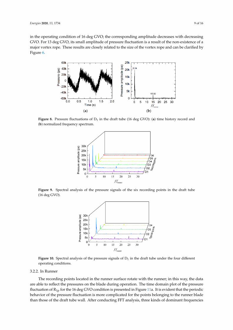
Figure 9 shows the normalized frequency spectrum obtained from D1 to D6 for 16 deg GVO.The pressure amplitude in each individual part of the draft tube (consisting of cone, elbow part,and diffuser) indicates that the amplitude in the draft tube cone is the largest; then, the pressureoscillation gradually weakens downstream. This phenomenon can be explained by the tangentialvelocity being largest in the cone area and decreasing downstream on account of viscous effects.Figure 10 presents the normalized frequency spectrum of D1 under the four different operatingconditions. It can be concluded that the pressure fluctuation of the draft tube reaches its maximum
Energies 2020, 13, 1734 9 of 16
in the operating condition of 16 deg GVO; the corresponding amplitude decreases with decreasingGVO. For 13 deg GVO, its small amplitude of pressure fluctuation is a result of the non-existence of amajor vortex rope. These results are closely related to the size of the vortex rope and can be clarified byFigure 6.
Energies 2020, 13, x FOR PEER REVIEW 9 of 16
Figure 9 shows the normalized frequency spectrum obtained from D1 to D6 for 16 deg GVO. The
pressure amplitude in each individual part of the draft tube (consisting of cone, elbow part, and
diffuser) indicates that the amplitude in the draft tube cone is the largest; then, the pressure oscillation
gradually weakens downstream. This phenomenon can be explained by the tangential velocity being
largest in the cone area and decreasing downstream on account of viscous effects. Figure 10 presents
the normalized frequency spectrum of D1 under the four different operating conditions. It can be
concluded that the pressure fluctuation of the draft tube reaches its maximum in the operating
condition of 16 deg GVO; the corresponding amplitude decreases with decreasing GVO. For 13 deg
GVO, its small amplitude of pressure fluctuation is a result of the non‐existence of a major vortex
rope. These results are closely related to the size of the vortex rope and can be clarified by Figure 6.
(a) (b)
Figure 8. Pressure fluctuations of D1 in the draft tube (16 deg GVO): (a) time history record and (b)
normalized frequency spectrum.
Figure 9. Spectral analysis of the pressure signals of the six recording points in the draft tube (16 deg
GVO).
Figure 10. Spectral analysis of the pressure signals of D1 in the draft tube under the four different
operating conditions.
Figure 8. Pressure fluctuations of D1 in the draft tube (16 deg GVO): (a) time history record and(b) normalized frequency spectrum.
Energies 2020, 13, x FOR PEER REVIEW 9 of 16
Figure 9 shows the normalized frequency spectrum obtained from D1 to D6 for 16 deg GVO. The
pressure amplitude in each individual part of the draft tube (consisting of cone, elbow part, and
diffuser) indicates that the amplitude in the draft tube cone is the largest; then, the pressure oscillation
gradually weakens downstream. This phenomenon can be explained by the tangential velocity being
largest in the cone area and decreasing downstream on account of viscous effects. Figure 10 presents
the normalized frequency spectrum of D1 under the four different operating conditions. It can be
concluded that the pressure fluctuation of the draft tube reaches its maximum in the operating
condition of 16 deg GVO; the corresponding amplitude decreases with decreasing GVO. For 13 deg
GVO, its small amplitude of pressure fluctuation is a result of the non‐existence of a major vortex
rope. These results are closely related to the size of the vortex rope and can be clarified by Figure 6.
(a) (b)
Figure 8. Pressure fluctuations of D1 in the draft tube (16 deg GVO): (a) time history record and (b)
normalized frequency spectrum.
Figure 9. Spectral analysis of the pressure signals of the six recording points in the draft tube (16 deg
GVO).
Figure 10. Spectral analysis of the pressure signals of D1 in the draft tube under the four different
operating conditions.
Figure 9. Spectral analysis of the pressure signals of the six recording points in the draft tube(16 deg GVO).
Energies 2020, 13, x FOR PEER REVIEW 9 of 16
Figure 9 shows the normalized frequency spectrum obtained from D1 to D6 for 16 deg GVO. The
pressure amplitude in each individual part of the draft tube (consisting of cone, elbow part, and
diffuser) indicates that the amplitude in the draft tube cone is the largest; then, the pressure oscillation
gradually weakens downstream. This phenomenon can be explained by the tangential velocity being
largest in the cone area and decreasing downstream on account of viscous effects. Figure 10 presents
the normalized frequency spectrum of D1 under the four different operating conditions. It can be
concluded that the pressure fluctuation of the draft tube reaches its maximum in the operating
condition of 16 deg GVO; the corresponding amplitude decreases with decreasing GVO. For 13 deg
GVO, its small amplitude of pressure fluctuation is a result of the non‐existence of a major vortex
rope. These results are closely related to the size of the vortex rope and can be clarified by Figure 6.
(a) (b)
Figure 8. Pressure fluctuations of D1 in the draft tube (16 deg GVO): (a) time history record and (b)
normalized frequency spectrum.
Figure 9. Spectral analysis of the pressure signals of the six recording points in the draft tube (16 deg
GVO).
Figure 10. Spectral analysis of the pressure signals of D1 in the draft tube under the four different
operating conditions.
Figure 10. Spectral analysis of the pressure signals of D1 in the draft tube under the four differentoperating conditions.
3.2.2. In Runner
The recording points located in the runner surface rotate with the runner; in this way, the dataare able to reflect the pressures on the blade during operation. The time domain plot of the pressurefluctuation of R1p for the 16 deg GVO condition is presented in Figure 11a. It is evident that the periodicbehavior of the pressure fluctuation is more complicated for the points belonging to the runner bladethan those of the draft tube wall. After conducting FFT analysis, three kinds of dominant frequencies
Energies 2020, 13, 1734 10 of 16
could be observed in Figure 11b. For the low frequencies of 0.24, 0.72, 0.96, and 1.92 times that ofthe runner rotational frequency, they correspond to the rotating vortex rope (RVR) frequency and itsharmonics. It is worth noting that the highest amplitude corresponds to the fourth harmonic of theRVR frequency. The high frequency of 15.0 times that of the runner rotational frequency pertains to theblade passing frequency. This RSI frequency (f runner) was also confirmed in the numerical simulationsof Francis turbines performed by Zhu et al. [30]. However, it could not be found in the numericalresults of Francis pump-turbines conducted by Trivedi [31]. The other high frequency of 24.0 timesthat of the runner rotational frequency belongs to the guide vane passing frequency. This particularRSI frequency (f gv) was also detected by Trivedi et al. [28,32].
Energies 2020, 13, x FOR PEER REVIEW 10 of 16
3.2.2. In Runner
The recording points located in the runner surface rotate with the runner; in this way, the data
are able to reflect the pressures on the blade during operation. The time domain plot of the pressure
fluctuation of R1p for the 16 deg GVO condition is presented in Figure 11a. It is evident that the
periodic behavior of the pressure fluctuation is more complicated for the points belonging to the
runner blade than those of the draft tube wall. After conducting FFT analysis, three kinds of dominant
frequencies could be observed in Figure 11b. For the low frequencies of 0.24, 0.72, 0.96, and 1.92 times
that of the runner rotational frequency, they correspond to the rotating vortex rope (RVR) frequency
and its harmonics. It is worth noting that the highest amplitude corresponds to the fourth harmonic
of the RVR frequency. The high frequency of 15.0 times that of the runner rotational frequency
pertains to the blade passing frequency. This RSI frequency (frunner) was also confirmed in the
numerical simulations of Francis turbines performed by Zhu et al. [30]. However, it could not be
found in the numerical results of Francis pump‐turbines conducted by Trivedi [31]. The other high
frequency of 24.0 times that of the runner rotational frequency belongs to the guide vane passing
frequency. This particular RSI frequency (fgv) was also detected by Trivedi et al. [28,32].
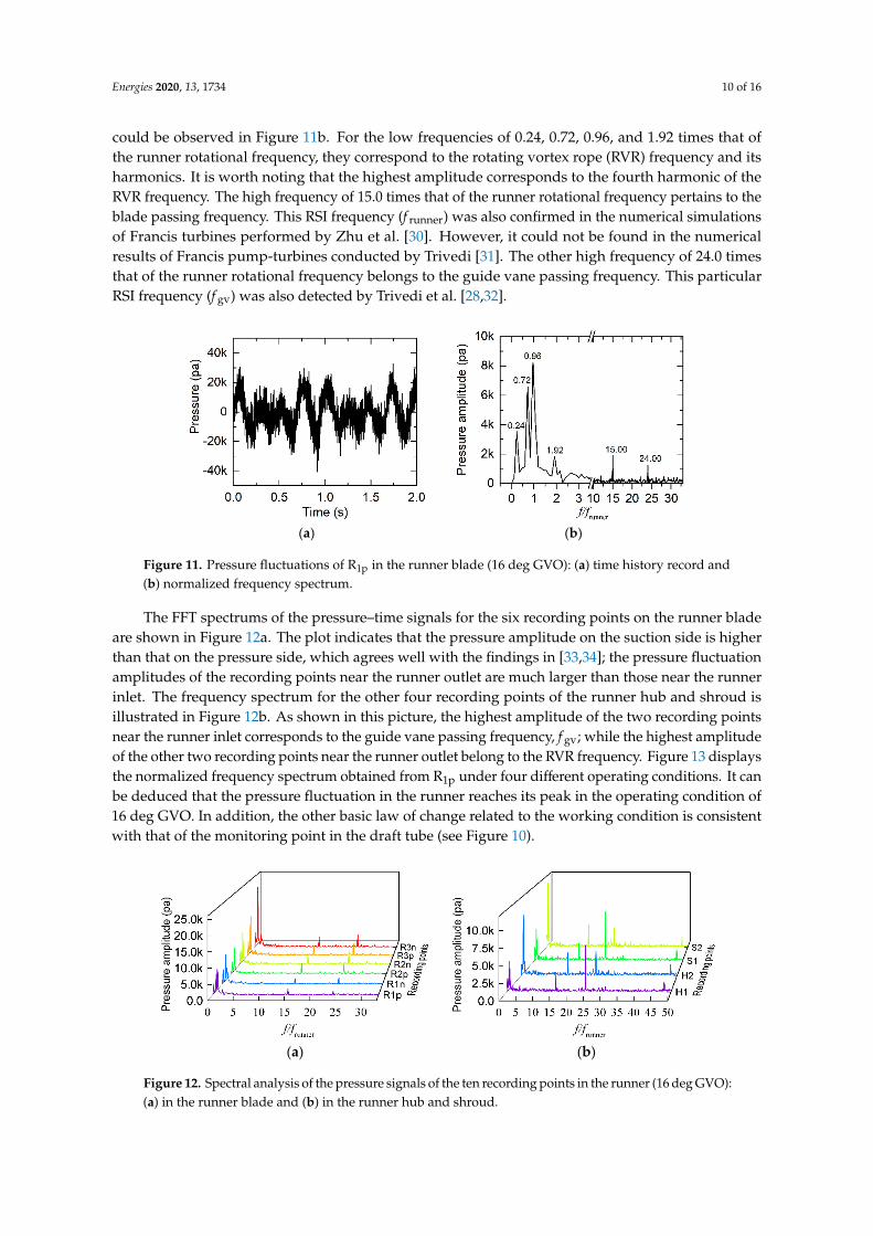
The FFT spectrums of the pressure–time signals for the six recording points on the runner blade
are shown in Figure 12a. The plot indicates that the pressure amplitude on the suction side is higher
than that on the pressure side, which agrees well with the findings in [33,34]; the pressure fluctuation
amplitudes of the recording points near the runner outlet are much larger than those near the runner
inlet. The frequency spectrum for the other four recording points of the runner hub and shroud is
illustrated in Figure 12b. As shown in this picture, the highest amplitude of the two recording points
near the runner inlet corresponds to the guide vane passing frequency, fgv; while the highest
amplitude of the other two recording points near the runner outlet belong to the RVR frequency.
Figure 13 displays the normalized frequency spectrum obtained from R1p under four different
operating conditions. It can be deduced that the pressure fluctuation in the runner reaches its peak
in the operating condition of 16 deg GVO. In addition, the other basic law of change related to the
working condition is consistent with that of the monitoring point in the draft tube (see Figure 10).
(a) (b)
Figure 11. Pressure fluctuations of R1p in the runner blade (16 deg GVO): (a) time history record and
(b) normalized frequency spectrum.
Figure 11. Pressure fluctuations of R1p in the runner blade (16 deg GVO): (a) time history record and(b) normalized frequency spectrum.
The FFT spectrums of the pressure–time signals for the six recording points on the runner bladeare shown in Figure 12a. The plot indicates that the pressure amplitude on the suction side is higherthan that on the pressure side, which agrees well with the findings in [33,34]; the pressure fluctuationamplitudes of the recording points near the runner outlet are much larger than those near the runnerinlet. The frequency spectrum for the other four recording points of the runner hub and shroud isillustrated in Figure 12b. As shown in this picture, the highest amplitude of the two recording pointsnear the runner inlet corresponds to the guide vane passing frequency, f gv; while the highest amplitudeof the other two recording points near the runner outlet belong to the RVR frequency. Figure 13 displaysthe normalized frequency spectrum obtained from R1p under four different operating conditions. It canbe deduced that the pressure fluctuation in the runner reaches its peak in the operating condition of16 deg GVO. In addition, the other basic law of change related to the working condition is consistentwith that of the monitoring point in the draft tube (see Figure 10).Energies 2020, 13, x FOR PEER REVIEW 11 of 16
(a) (b)
Figure 12. Spectral analysis of the pressure signals of the ten recording points in the runner (16 deg
GVO): (a) in the runner blade and (b) in the runner hub and shroud.
Figure 13. Spectral analysis of the pressure signals of R1p in the runner under the four different
operating conditions.
3.2.3. In Vaneless Space
The diagrams regarding the time and frequency domain of the pressure fluctuation for V1 are
displayed in Figure 14, respectively. The highest amplitude corresponds to the runner blade passing
frequency, and the second highest amplitude is the RVR frequency. These two frequencies were also
observed in the calculation of Francis pump‐turbines performed by Iliev et al. [35]; whereas, only 15.0
times that of the runner rotational frequency was reported in some of the papers by Trivedi et al. [36–
38]. Based on the simulation results in this study, it can be concluded that the pressure wave of RVR
is able to travel upstream (from the draft tube domain to the runner domain, and then to vaneless
space), although the amplitude of fluctuation decreases, indicating that the oscillating intensity
gradually recedes. Finally, the recording points in the vaneless space have the lowest peak pressure
amplitude compared to those of the runner blade and the draft tube wall. Figure 15 shows the
normalized frequency spectrum obtained from V1 under the four different operating conditions,
which reveals that there is not much difference between the various operating points in terms of the
highest amplitude of pressure fluctuation.
Figure 12. Spectral analysis of the pressure signals of the ten recording points in the runner (16 deg GVO):(a) in the runner blade and (b) in the runner hub and shroud.
Energies 2020, 13, 1734 11 of 16
Energies 2020, 13, x FOR PEER REVIEW 11 of 16
(a) (b)
Figure 12. Spectral analysis of the pressure signals of the ten recording points in the runner (16 deg
GVO): (a) in the runner blade and (b) in the runner hub and shroud.
Figure 13. Spectral analysis of the pressure signals of R1p in the runner under the four different
operating conditions.
3.2.3. In Vaneless Space
The diagrams regarding the time and frequency domain of the pressure fluctuation for V1 are
displayed in Figure 14, respectively. The highest amplitude corresponds to the runner blade passing
frequency, and the second highest amplitude is the RVR frequency. These two frequencies were also
observed in the calculation of Francis pump‐turbines performed by Iliev et al. [35]; whereas, only 15.0
times that of the runner rotational frequency was reported in some of the papers by Trivedi et al. [36–
38]. Based on the simulation results in this study, it can be concluded that the pressure wave of RVR
is able to travel upstream (from the draft tube domain to the runner domain, and then to vaneless
space), although the amplitude of fluctuation decreases, indicating that the oscillating intensity
gradually recedes. Finally, the recording points in the vaneless space have the lowest peak pressure
amplitude compared to those of the runner blade and the draft tube wall. Figure 15 shows the
normalized frequency spectrum obtained from V1 under the four different operating conditions,
which reveals that there is not much difference between the various operating points in terms of the
highest amplitude of pressure fluctuation.
Figure 13. Spectral analysis of the pressure signals of R1p in the runner under the four differentoperating conditions.
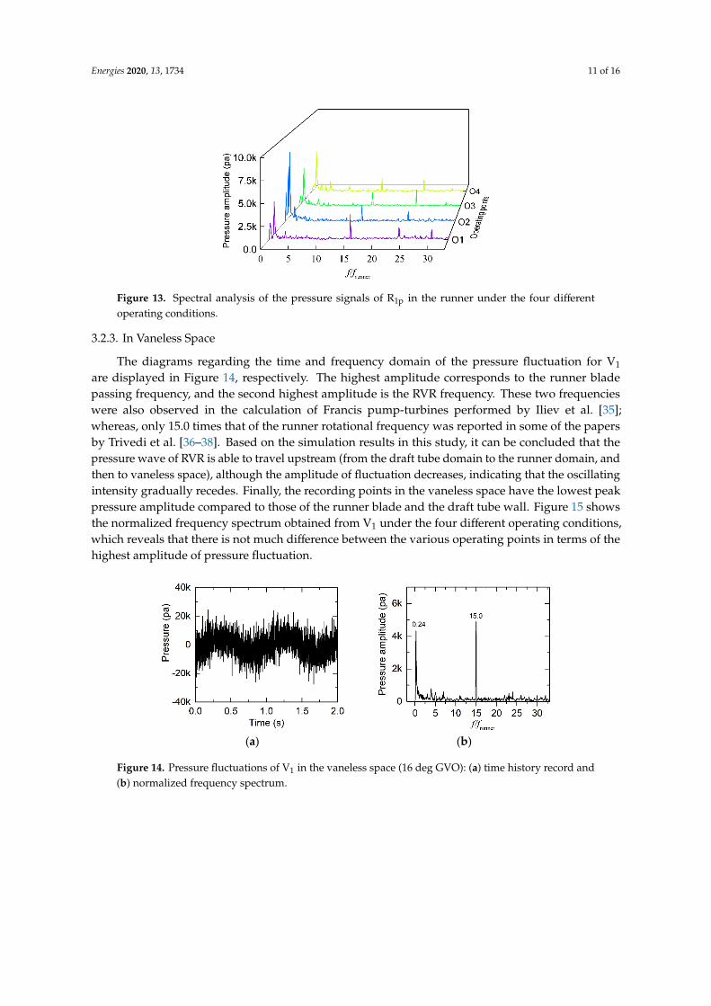
3.2.3. In Vaneless Space
The diagrams regarding the time and frequency domain of the pressure fluctuation for V1
are displayed in Figure 14, respectively. The highest amplitude corresponds to the runner bladepassing frequency, and the second highest amplitude is the RVR frequency. These two frequencieswere also observed in the calculation of Francis pump-turbines performed by Iliev et al. [35];whereas, only 15.0 times that of the runner rotational frequency was reported in some of the papersby Trivedi et al. [36–38]. Based on the simulation results in this study, it can be concluded that thepressure wave of RVR is able to travel upstream (from the draft tube domain to the runner domain, andthen to vaneless space), although the amplitude of fluctuation decreases, indicating that the oscillatingintensity gradually recedes. Finally, the recording points in the vaneless space have the lowest peakpressure amplitude compared to those of the runner blade and the draft tube wall. Figure 15 showsthe normalized frequency spectrum obtained from V1 under the four different operating conditions,which reveals that there is not much difference between the various operating points in terms of thehighest amplitude of pressure fluctuation.Energies 2020, 13, x FOR PEER REVIEW 12 of 16
(a) (b)
Figure 14. Pressure fluctuations of V1 in the vaneless space (16 deg GVO): (a) time history record and
(b) normalized frequency spectrum.
Figure 15. Spectral analysis of the pressure signals of V1 in the vaneless space under the four different
operating conditions.
3.3. Hydraulic Axial Thrust
The pulsating hydraulic axial thrust is transmitted to the load‐bearing frame base of the
powerhouse via thrust bearing, and consequently poses a threat to the bearing and the powerhouse
structure. During certain transition processes, accidental lifting of the rotating part will occur when
the thrust bearing is subjected to upward force; on the other hand, excessive downward load on the
thrust bearing may increase the temperature of the thrust bearing pads, thus causing damage to them
[39]. In addition, the pulsation characteristics of axial hydraulic thrust make it one of the main sources
of noise and strong vibration occurring in the powerhouse structure. There are many hydropower
plants where prominent vibration problems frequently take place during off‐design and transient
operations, such as the Three Gorges Hydropower Station, the Ertan Hydropower Station, and the
Guangzhou Pumped‐Storage Power Station [40,41]; therefore, it is necessary to explore, in depth, and
understand the pulsation properties of the hydraulic axial thrust of Francis turbines.
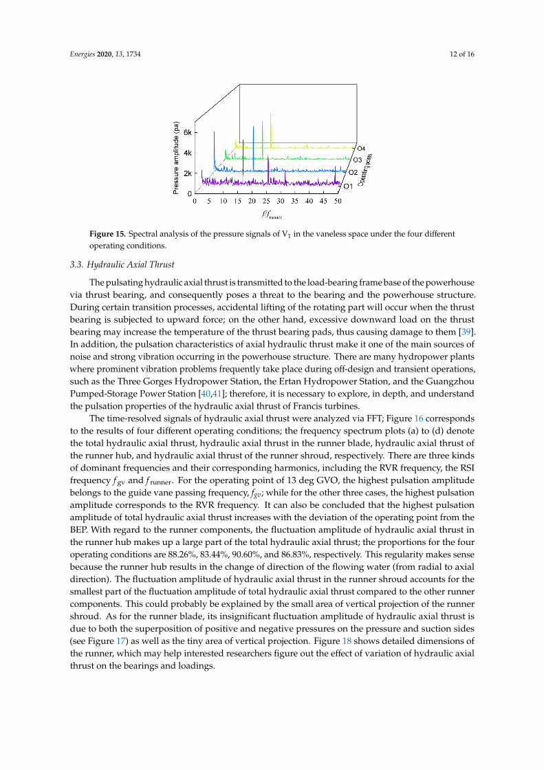
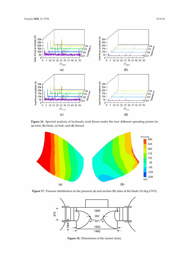
The time‐resolved signals of hydraulic axial thrust were analyzed via FFT; Figure 16 corresponds
to the results of four different operating conditions; the frequency spectrum plots (a) to (d) denote
the total hydraulic axial thrust, hydraulic axial thrust in the runner blade, hydraulic axial thrust of
the runner hub, and hydraulic axial thrust of the runner shroud, respectively. There are three kinds
of dominant frequencies and their corresponding harmonics, including the RVR frequency, the RSI
frequency fgv and frunner. For the operating point of 13 deg GVO, the highest pulsation amplitude
belongs to the guide vane passing frequency, fgv; while for the other three cases, the highest pulsation
amplitude corresponds to the RVR frequency. It can also be concluded that the highest pulsation
amplitude of total hydraulic axial thrust increases with the deviation of the operating point from the
BEP. With regard to the runner components, the fluctuation amplitude of hydraulic axial thrust in
the runner hub makes up a large part of the total hydraulic axial thrust; the proportions for the four
Figure 14. Pressure fluctuations of V1 in the vaneless space (16 deg GVO): (a) time history record and(b) normalized frequency spectrum.
Energies 2020, 13, 1734 12 of 16
Energies 2020, 13, x FOR PEER REVIEW 12 of 16
(a) (b)
Figure 14. Pressure fluctuations of V1 in the vaneless space (16 deg GVO): (a) time history record and
(b) normalized frequency spectrum.
Figure 15. Spectral analysis of the pressure signals of V1 in the vaneless space under the four different
operating conditions.
3.3. Hydraulic Axial Thrust
The pulsating hydraulic axial thrust is transmitted to the load‐bearing frame base of the
powerhouse via thrust bearing, and consequently poses a threat to the bearing and the powerhouse
structure. During certain transition processes, accidental lifting of the rotating part will occur when
the thrust bearing is subjected to upward force; on the other hand, excessive downward load on the
thrust bearing may increase the temperature of the thrust bearing pads, thus causing damage to them
[39]. In addition, the pulsation characteristics of axial hydraulic thrust make it one of the main sources
of noise and strong vibration occurring in the powerhouse structure. There are many hydropower
plants where prominent vibration problems frequently take place during off‐design and transient
operations, such as the Three Gorges Hydropower Station, the Ertan Hydropower Station, and the
Guangzhou Pumped‐Storage Power Station [40,41]; therefore, it is necessary to explore, in depth, and
understand the pulsation properties of the hydraulic axial thrust of Francis turbines.
The time‐resolved signals of hydraulic axial thrust were analyzed via FFT; Figure 16 corresponds
to the results of four different operating conditions; the frequency spectrum plots (a) to (d) denote
the total hydraulic axial thrust, hydraulic axial thrust in the runner blade, hydraulic axial thrust of
the runner hub, and hydraulic axial thrust of the runner shroud, respectively. There are three kinds
of dominant frequencies and their corresponding harmonics, including the RVR frequency, the RSI
frequency fgv and frunner. For the operating point of 13 deg GVO, the highest pulsation amplitude
belongs to the guide vane passing frequency, fgv; while for the other three cases, the highest pulsation
amplitude corresponds to the RVR frequency. It can also be concluded that the highest pulsation
amplitude of total hydraulic axial thrust increases with the deviation of the operating point from the
BEP. With regard to the runner components, the fluctuation amplitude of hydraulic axial thrust in
the runner hub makes up a large part of the total hydraulic axial thrust; the proportions for the four
Figure 15. Spectral analysis of the pressure signals of V1 in the vaneless space under the four differentoperating conditions.
3.3. Hydraulic Axial Thrust
The pulsating hydraulic axial thrust is transmitted to the load-bearing frame base of the powerhousevia thrust bearing, and consequently poses a threat to the bearing and the powerhouse structure.During certain transition processes, accidental lifting of the rotating part will occur when the thrustbearing is subjected to upward force; on the other hand, excessive downward load on the thrustbearing may increase the temperature of the thrust bearing pads, thus causing damage to them [39].In addition, the pulsation characteristics of axial hydraulic thrust make it one of the main sources ofnoise and strong vibration occurring in the powerhouse structure. There are many hydropower plantswhere prominent vibration problems frequently take place during off-design and transient operations,such as the Three Gorges Hydropower Station, the Ertan Hydropower Station, and the GuangzhouPumped-Storage Power Station [40,41]; therefore, it is necessary to explore, in depth, and understandthe pulsation properties of the hydraulic axial thrust of Francis turbines.
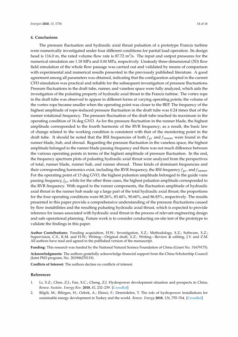
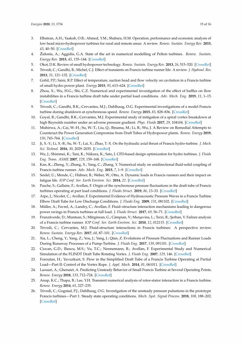
The time-resolved signals of hydraulic axial thrust were analyzed via FFT; Figure 16 correspondsto the results of four different operating conditions; the frequency spectrum plots (a) to (d) denotethe total hydraulic axial thrust, hydraulic axial thrust in the runner blade, hydraulic axial thrust ofthe runner hub, and hydraulic axial thrust of the runner shroud, respectively. There are three kindsof dominant frequencies and their corresponding harmonics, including the RVR frequency, the RSIfrequency f gv and f runner. For the operating point of 13 deg GVO, the highest pulsation amplitudebelongs to the guide vane passing frequency, fgv; while for the other three cases, the highest pulsationamplitude corresponds to the RVR frequency. It can also be concluded that the highest pulsationamplitude of total hydraulic axial thrust increases with the deviation of the operating point from theBEP. With regard to the runner components, the fluctuation amplitude of hydraulic axial thrust inthe runner hub makes up a large part of the total hydraulic axial thrust; the proportions for the fouroperating conditions are 88.26%, 83.44%, 90.60%, and 86.83%, respectively. This regularity makes sensebecause the runner hub results in the change of direction of the flowing water (from radial to axialdirection). The fluctuation amplitude of hydraulic axial thrust in the runner shroud accounts for thesmallest part of the fluctuation amplitude of total hydraulic axial thrust compared to the other runnercomponents. This could probably be explained by the small area of vertical projection of the runnershroud. As for the runner blade, its insignificant fluctuation amplitude of hydraulic axial thrust isdue to both the superposition of positive and negative pressures on the pressure and suction sides(see Figure 17) as well as the tiny area of vertical projection. Figure 18 shows detailed dimensions ofthe runner, which may help interested researchers figure out the effect of variation of hydraulic axialthrust on the bearings and loadings.
Energies 2020, 13, 1734 13 of 16
Energies 2020, 13, x FOR PEER REVIEW 13 of 16
operating conditions are 88.26%, 83.44%, 90.60%, and 86.83%, respectively. This regularity makes
sense because the runner hub results in the change of direction of the flowing water (from radial to
axial direction). The fluctuation amplitude of hydraulic axial thrust in the runner shroud accounts
for the smallest part of the fluctuation amplitude of total hydraulic axial thrust compared to the other
runner components. This could probably be explained by the small area of vertical projection of the
runner shroud. As for the runner blade, its insignificant fluctuation amplitude of hydraulic axial
thrust is due to both the superposition of positive and negative pressures on the pressure and suction
sides (see Figure 17) as well as the tiny area of vertical projection. Figure 18 shows detailed
dimensions of the runner, which may help interested researchers figure out the effect of variation of
hydraulic axial thrust on the bearings and loadings.
(a) (b)
(c) (d)
Figure 16. Spectral analysis of hydraulic axial thrust under the four different operating points for (a)
total, (b) blade, (c) hub, and (d) shroud.
(a) (b)
Figure 17. Pressure distribution on the pressure (a) and suction (b) sides of the blade (16 deg GVO).
Figure 16. Spectral analysis of hydraulic axial thrust under the four different operating points for(a) total, (b) blade, (c) hub, and (d) shroud.
Energies 2020, 13, x FOR PEER REVIEW 13 of 16
operating conditions are 88.26%, 83.44%, 90.60%, and 86.83%, respectively. This regularity makes
sense because the runner hub results in the change of direction of the flowing water (from radial to
axial direction). The fluctuation amplitude of hydraulic axial thrust in the runner shroud accounts
for the smallest part of the fluctuation amplitude of total hydraulic axial thrust compared to the other
runner components. This could probably be explained by the small area of vertical projection of the
runner shroud. As for the runner blade, its insignificant fluctuation amplitude of hydraulic axial
thrust is due to both the superposition of positive and negative pressures on the pressure and suction
sides (see Figure 17) as well as the tiny area of vertical projection. Figure 18 shows detailed
dimensions of the runner, which may help interested researchers figure out the effect of variation of
hydraulic axial thrust on the bearings and loadings.
(a) (b)
(c) (d)
Figure 16. Spectral analysis of hydraulic axial thrust under the four different operating points for (a)
total, (b) blade, (c) hub, and (d) shroud.
(a) (b)
Figure 17. Pressure distribution on the pressure (a) and suction (b) sides of the blade (16 deg GVO). Figure 17. Pressure distribution on the pressure (a) and suction (b) sides of the blade (16 deg GVO).Energies 2020, 13, x FOR PEER REVIEW 14 of 16
Figure 18. Dimensions of the runner (mm).
4. Conclusions
The pressure fluctuation and hydraulic axial thrust pulsation of a prototype Francis turbine were
numerically investigated under four different conditions for partial load operation. Its design head
is 116.0 m, the rated volume flow rate is 87.72 m3/s. The input and output pressures for the numerical
simulation are 1.18 MPa and 0.04 MPa, respectively. Unsteady three‐dimensional (3D) flow field
simulation of the whole flow passage was carried out and validated by means of comparison with
experimental and numerical results presented in the previously published literature. A good
agreement among all parameters was obtained, indicating that the configuration adopted in the
current CFD simulation was practical and reliable for the subsequent investigation of pressure
fluctuations. Pressure fluctuations in the draft tube, runner, and vaneless space were fully analyzed,
which aids the investigation of the pulsating property of hydraulic axial thrust in the Francis turbine.
The vortex rope in the draft tube was observed to appear in different forms at varying operating
points; the volume of the vortex rope became smaller when the operating point was closer to the BEP.
The frequency of the highest amplitude of rope‐induced pressure fluctuation in the draft tube was
0.24 times that of the runner rotational frequency. The pressure fluctuation of the draft tube reached
its maximum in the operating condition of 16 deg GVO. As for the pressure fluctuation in the runner
blade, the highest amplitude corresponded to the fourth harmonic of the RVR frequency; as a result,
the basic law of change related to the working condition is consistent with that of the monitoring
point in the draft tube. It should be noted that the RSI frequencies of both fgv and frunner were found in
the runner blade, hub, and shroud. Regarding the pressure fluctuation in the vaneless space, the
highest amplitude belonged to the runner blade passing frequency and there was not much difference
between the various operating points in terms of the highest amplitude of pressure fluctuation. In the
end, the frequency spectrum plots of pulsating hydraulic axial thrust were analyzed from the
perspectives of total, runner blade, runner hub, and runner shroud. Three kinds of dominant
frequencies and their corresponding harmonics exist, including the RVR frequency, the RSI frequency
fgv, and frunner. For the operating point of 13 deg GVO, the highest pulsation amplitude belonged to the
guide vane passing frequency, fgv, while for the other three cases, the highest pulsation amplitude
corresponded to the RVR frequency. With regard to the runner components, the fluctuation
amplitude of hydraulic axial thrust in the runner hub made up a large part of the total hydraulic axial
thrust; the proportions for the four operating conditions were 88.26%, 83.44%, 90.60%, and 86.83%,
respectively. The results presented in this paper provide a comprehensive understanding of the
pressure fluctuations caused by flow instabilities and the resulting pulsating hydraulic axial thrust,
which is expected to provide reference for issues associated with hydraulic axial thrust in the process
of relevant engineering design and safe operational planning. Future work is to consider conducting
on‐site test of the prototype to validate the findings in this paper.
Supervision, C.S., K.M. and H.W.; Writing—Original draft, X.Z.; Writing—Review & editing, J.Y. and Z.M.
Funding: This research was funded by the National Natural Science Foundation of China (Grant No. 51679175).
Figure 18. Dimensions of the runner (mm).
Energies 2020, 13, 1734 14 of 16
4. Conclusions
The pressure fluctuation and hydraulic axial thrust pulsation of a prototype Francis turbinewere numerically investigated under four different conditions for partial load operation. Its designhead is 116.0 m, the rated volume flow rate is 87.72 m3/s. The input and output pressures for thenumerical simulation are 1.18 MPa and 0.04 MPa, respectively. Unsteady three-dimensional (3D) flowfield simulation of the whole flow passage was carried out and validated by means of comparisonwith experimental and numerical results presented in the previously published literature. A goodagreement among all parameters was obtained, indicating that the configuration adopted in the currentCFD simulation was practical and reliable for the subsequent investigation of pressure fluctuations.Pressure fluctuations in the draft tube, runner, and vaneless space were fully analyzed, which aids theinvestigation of the pulsating property of hydraulic axial thrust in the Francis turbine. The vortex ropein the draft tube was observed to appear in different forms at varying operating points; the volume ofthe vortex rope became smaller when the operating point was closer to the BEP. The frequency of thehighest amplitude of rope-induced pressure fluctuation in the draft tube was 0.24 times that of therunner rotational frequency. The pressure fluctuation of the draft tube reached its maximum in theoperating condition of 16 deg GVO. As for the pressure fluctuation in the runner blade, the highestamplitude corresponded to the fourth harmonic of the RVR frequency; as a result, the basic lawof change related to the working condition is consistent with that of the monitoring point in thedraft tube. It should be noted that the RSI frequencies of both f gv and f runner were found in therunner blade, hub, and shroud. Regarding the pressure fluctuation in the vaneless space, the highestamplitude belonged to the runner blade passing frequency and there was not much difference betweenthe various operating points in terms of the highest amplitude of pressure fluctuation. In the end,the frequency spectrum plots of pulsating hydraulic axial thrust were analyzed from the perspectivesof total, runner blade, runner hub, and runner shroud. Three kinds of dominant frequencies andtheir corresponding harmonics exist, including the RVR frequency, the RSI frequency f gv, and f runner.For the operating point of 13 deg GVO, the highest pulsation amplitude belonged to the guide vanepassing frequency, fgv, while for the other three cases, the highest pulsation amplitude corresponded tothe RVR frequency. With regard to the runner components, the fluctuation amplitude of hydraulicaxial thrust in the runner hub made up a large part of the total hydraulic axial thrust; the proportionsfor the four operating conditions were 88.26%, 83.44%, 90.60%, and 86.83%, respectively. The resultspresented in this paper provide a comprehensive understanding of the pressure fluctuations causedby flow instabilities and the resulting pulsating hydraulic axial thrust, which is expected to providereference for issues associated with hydraulic axial thrust in the process of relevant engineering designand safe operational planning. Future work is to consider conducting on-site test of the prototype tovalidate the findings in this paper.
Author Contributions: Funding acquisition, H.W.; Investigation, X.Z.; Methodology, X.Z.; Software, X.Z.;Supervision, C.S., K.M. and H.W.; Writing—Original draft, X.Z.; Writing—Review & editing, J.Y. and Z.M.All authors have read and agreed to the published version of the manuscript.
Funding: This research was funded by the National Natural Science Foundation of China (Grant No. 51679175).
Acknowledgments: The authors gratefully acknowledge financial support from the China Scholarship Council(Joint PhD program, No. 201906270119).
Conflicts of Interest: The authors declare no conflicts of interest.
References
1. Li, X.Z.; Chen, Z.J.; Fan, X.C.; Cheng, Z.J. Hydropower development situation and prospects in China.Renew. Sustain. Energy Rev. 2018, 82, 232–239. [CrossRef]
2. Bilgili, M.; Bilirgen, H.; Ozbek, A.; Ekinci, F.; Demirdelen, T. The role of hydropower installations forsustainable energy development in Turkey and the world. Renew. Energy 2018, 126, 755–764. [CrossRef]
3. Elbatran, A.H.; Yaakob, O.B.; Ahmed, Y.M.; Shabara, H.M. Operation, performance and economic analysis oflow head micro-hydropower turbines for rural and remote areas: A review. Renew. Sustain. Energy Rev. 2015,43, 40–50. [CrossRef]
4. Židonis, A.; Aggidis, G.A. State of the art in numerical modelling of Pelton turbines. Renew. Sustain.Energy Rev. 2015, 45, 135–144. [CrossRef]
5. Okot, D.K. Review of small hydropower technology. Renew. Sustain. Energy Rev. 2013, 26, 515–520. [CrossRef]6. Trivedi, C.; Gandhi, B.; Michel, C.J. Effect of transients on Francis turbine runner life: A review. J. Hydraul. Res.
2013, 51, 121–132. [CrossRef]7. Gohil, P.P.; Saini, R.P. Effect of temperature, suction head and flow velocity on cavitation in a Francis turbine
of small hydro power plant. Energy 2015, 93, 613–624. [CrossRef]8. Zhou, X.; Wu, H.G.; Shi, C.Z. Numerical and experimental investigation of the effect of baffles on flow
instabilities in a Francis turbine draft tube under partial load conditions. Adv. Mech. Eng. 2019, 11, 1–15.[CrossRef]
9. Trivedi, C.; Gandhi, B.K.; Cervantes, M.J.; Dahlhaug, O.G. Experimental investigations of a model Francisturbine during shutdown at synchronous speed. Renew. Energy 2015, 83, 828–836. [CrossRef]
10. Goyal, R.; Gandhi, B.K.; Cervantes, M.J. Experimental study of mitigation of a spiral vortex breakdown athigh Reynolds number under an adverse pressure gradient. Phys. Fluids 2017, 29, 104104. [CrossRef]
11. Muhirwa, A.; Cai, W.-H.; Su, W.-T.; Liu, Q.; Binama, M.; Li, B.; Wu, J. A Review on Remedial Attempts toCounteract the Power Generation Compromise from Draft Tubes of Hydropower plants. Renew. Energy 2019,150, 743–764. [CrossRef]
12. Ji, X.-Y.; Li, X.-B.; Su, W.-T.; Lai, X.; Zhao, T.-X. On the hydraulic axial thrust of Francis hydro-turbine. J. Mech.Sci. Technol. 2016, 30, 2029–2035. [CrossRef]
13. Wu, J.; Shimmei, K.; Tani, K.; Niikura, K.; Sato, J. CFD-based design optimization for hydro turbines. J. FluidsEng. Trans. ASME 2007, 129, 159–168. [CrossRef]
14. Kan, K.; Zheng, Y.; Zhang, X.; Yang, C.; Zhang, Y. Numerical study on unidirectional fluid-solid coupling ofFrancis turbine runner. Adv. Mech. Eng. 2015, 7, 1–9. [CrossRef]
15. Seidel, U.; Mende, C.; Hübner, B.; Weber, W.; Otto, A. Dynamic loads in Francis runners and their impact onfatigue life. IOP Conf. Ser. Earth Environ. Sci. 2014, 22. [CrossRef]
16. Pasche, S.; Gallaire, F.; Avellan, F. Origin of the synchronous pressure fluctuations in the draft tube of Francisturbines operating at part load conditions. J. Fluids Struct. 2019, 86, 13–33. [CrossRef]
17. Arpe, J.; Nicolet, C.; Avellan, F. Experimental Evidence of Hydroacoustic Pressure Waves in a Francis TurbineElbow Draft Tube for Low Discharge Conditions. J. Fluids Eng. 2009, 131, 081102. [CrossRef]
18. Müller, A.; Favrel, A.; Landry, C.; Avellan, F. Fluid–structure interaction mechanisms leading to dangerouspower swings in Francis turbines at full load. J. Fluids Struct. 2017, 69, 56–71. [CrossRef]
20. Trivedi, C.; Cervantes, M.J. Fluid-structure interactions in Francis turbines: A perspective review.Renew. Sustain. Energy Rev. 2017, 68, 87–101. [CrossRef]
21. Xia, L.; Cheng, Y.; Yang, Z.; You, J.; Yang, J.; Qian, Z. Evolutions of Pressure Fluctuations and Runner LoadsDuring Runaway Processes of a Pump-Turbine. J. Fluids Eng. 2017, 139, 091101. [CrossRef]
22. Ciocan, G.D.; Iliescu, M.S.; Vu, T.C.; Nennemann, B.; Avellan, F. Experimental Study and NumericalSimulation of the FLINDT Draft Tube Rotating Vortex. J. Fluids Eng. 2007, 129, 146. [CrossRef]
23. Foroutan, H.; Yavuzkurt, S. Flow in the Simplified Draft Tube of a Francis Turbine Operating at PartialLoad—Part II: Control of the Vortex Rope. J. Appl. Mech. 2014, 81, 061011. [CrossRef]
24. Laouari, A.; Ghenaiet, A. Predicting Unsteady Behavior of Small Francis Turbine at Several Operating Points.Renew. Energy 2018, 133, 712–724. [CrossRef]
25. Anup, K.C.; Thapa, B.; Lee, Y.H. Transient numerical analysis of rotor-stator interaction in a Francis turbine.Renew. Energy 2014, 65, 227–235.
26. Trivedi, C.; Gogstad, P.J.; Dahlhaug, O.G. Investigation of the unsteady pressure pulsations in the prototypeFrancis turbines—Part 1: Steady state operating conditions. Mech. Syst. Signal Process. 2018, 108, 188–202.[CrossRef]
27. Trivedi, C.; Gogstad, P.J.; Dahlhaug, O.G.; Trivedi, C.; Gogstad, J.; Dahlhaug, O.G. Investigation of theunsteady pressure pulsations in the prototype Francis turbines during load variation and startup. J. Renew.Sustain. Energy 2017, 9, 064502. [CrossRef]
28. Trivedi, C.; Cervantes, M.J.; Gandhi, B.K. Investigation of a high head Francis turbine at runaway operatingconditions. Energies 2016, 9, 149. [CrossRef]
29. Trivedi, C.; Cervantes, M.J.; Gandhi, B.K.; Dahlhaug, O.G. Experimental and Numerical Studies for a HighHead Francis Turbine at Several Operating Points. J. Fluids Eng. 2013, 135, 111102. [CrossRef]
30. Zhu, D.; Tao, R.; Xiao, R.; Pan, L. Solving the runner blade crack problem for a Francis hydro-turbineoperating under condition-complexity. Renew. Energy 2020, 149, 298–320. [CrossRef]
31. Trivedi, C.; Agnalt, E.; Dahlhaug, O.G. Investigations of unsteady pressure loading in a Francis turbineduring variable-speed operation. Renew. Energy 2017, 113, 397–410. [CrossRef]
32. Trivedi, C.; Dahlhaug, O.G. Interaction between trailing edge wake and vortex rings in a Francis turbine atrunaway condition: Compressible large eddy simulation. Phys. Fluids 2018, 30, 075101. [CrossRef]
33. Wang, Z.; Zhou, L. Simulations and measurements of pressure oscillations caused by vortex ropes. J. FluidsEng. Trans. ASME 2006, 128, 649–655. [CrossRef]
34. Gao, Z.; Zhu, W.; Meng, L.; Zhang, J.; Zhang, F.; Pan, L.; Lu, L. Experimental Study of the FrancisTurbine Pressure Fluctuations and the Pressure Fluctuations Superposition Phenomenon Inside the Runner.J. Fluids Eng. 2018, 140, 1–9. [CrossRef]
35. Iliev, I.; Trivedi, C.; Agnalt, E.; Dahlhaug, O.G. Variable-speed operation and pressure pulsations in a Francisturbine and a pump-turbine. IOP Conf. Ser. Earth Environ. Sci. 2019, 240, 072034. [CrossRef]
36. Trivedi, C.; Cervantes, M.J.; Gandhi, B.K.; Dahlhaug, O.G. Transient Pressure Measurements on a High HeadModel Francis Turbine During Emergency Shutdown, Total Load Rejection, and Runaway. J. Fluids Eng.2014, 136, 121107. [CrossRef]
37. Trivedi, C.; Cervantes, M.J.; Dahlhaug, O.G. Experimental and numerical studies of a high-head Francisturbine: A review of the Francis-99 test case. Energies 2016, 9, 74. [CrossRef]
38. Trivedi, C. Investigations of Compressible Turbulent Flow in a High-Head Francis Turbine. J. Fluids Eng.Trans. ASME 2018, 140, 1–17. [CrossRef]
39. Xing, Z.; Hegao, W.; Kai, S. Overview and discussion on hydraulic axial thrust in Francis turbine research.J. Hydraul. Eng. 2019, 50, 1242–1252.
40. Zhang, C.H.; Zhang, Y.L. Nonlinear dynamic analysis of the Three Gorge Project powerhouse excited bypressure fluctuation. J. Zhejiang Univ. Sci. A 2009, 10, 1231–1240. [CrossRef]
41. Hegao, W.; Xing, Z.; Xing, Z.; Zhimin, Z. Flow-induced vibration analysis of hydropower plant under twotransfer paths. J. Huazhong Univ. Sci. Technol. Sci. Ed. 2020, 48, 1–6.