64
Hydraulic fracturing for shale gas in the UK Examining the evidence for potential environmental impacts Working in partnership
Hydraulic fracturing for shale gas in the UK Examining the evidence for potential environmental impacts
Working in partnership
Hydraulic fracturing for shale gas in the UK: evidence report 2
Hydraulic fracturing for shale gas in the UK: Examining the evidence for potential environmental impacts Main authors: Veronika Moore*, Alison Beresford** and Benedict Gove*
With contributions from: Ralph Underhill†, Sharolyn Parnham*, Helen Crow*, Robert Cunningham*, Harry Huyton*, Jeremy Sutton***, Tim Melling***,
Petra Billings‡ and Martin Salter¥.
* RSPB, UK Headquarters, The Lodge, Sandy, Bedfordshire SG19 2DL
** RSPB, Scotland Headquarters, 2 Lochside View, Edinburgh Park, Edinburgh EH12 9DH
*** RSPB, Northern England Region, 7.3.1 Cameron House, White Cross Estate, Lancaster LA1 4XF
† Current address: Public Interest Research Centre, Plas Drive, Machynlleth, Powys SY20 8ER
‡ Sussex Wildlife Trust, Woods Mill, Henfield, West Sussex BN5 9SD
¥Angling Trust, Eastwood House, 6 Rainbow Street, Leominster, Herefordshire HR6 8DQ
Issued: March 2014
© The Royal Society for the Protection of Birds 2014
Independent peer review of the science case was provided by Dr. Andrew Singer at the NERC Centre for Ecology & Hydrology, however, the opinions expressed are solely those of the RSPB
and partner organisations (namely Angling Trust, National Trust, Salmon & Trout Association, The Wildlife Trusts and Wildfowl & Wetlands Trust).
Citation: Moore, V., Beresford, A., & Gove, B. (2014) Hydraulic fracturing for shale gas in the UK: Examining the evidence for potential environmental impacts.
Sandy, Bedfordshire, UK: RSPB.
This document can be viewed online or downloaded at:
rspb.org.uk/fracking
For further information, contact:
Hydraulic fracturing for shale gas in the UK: evidence report 3
Table of contentsExecutive summary 6
1. Shale gas extraction in the UK 8
1.1. Shale gas deposits and high-volume hydraulic fracturing 8
1.2. Shale reserves, licensing and planning in the UK 9
2. Types of environmental risks and their management 12
3. Impacts on the water environment 13
3.1. Groundwater vulnerability 13
3.2. Polluting potential of fracking fluid 15
3.3. Water Usage 17
3.3.1. Analysis of water resource impacts in England and Wales 18
3.4. Flowback water management 21
3.5. Blowouts 23
3.6. Induced seismicity 23
3.7. Well decommissioning 24
4. Ecological Impacts 26
4.1. Habitat loss and fragmentation 26
4.1.1. Analysis of impacts on UK protected areas and species 28
4.1.2 Case study: Potential impacts of shale gas development on the population of pink-footed geese in and around the Ribble and Alt Estuaries SPA 30
4.2. Disturbance effects 32
4.2.1. Case study: Potential impacts of light pollution on barbastelle bats 36
4.3. Impacts on aquatic biodiversity 39
4.3.1 Case study: Potential impacts on chalk streams 40
5. Climate change impacts 42
5.1. Greenhouse gas emissions 42
6. Current regulation and enforcement in Great Britain 45
6.1. Environmental monitoring 46
Conclusion 47
References 48
List of abbreviations 54
Annex 1: Summary of datasets used for mapping analysis 56
Annex 2: Methodology for the water availability mapping component 57
Annex 3: Sensitivity mapping for bird disturbance impacts 58
Hydraulic fracturing for shale gas in the UK: evidence report 4
Figure 1: Simple schematic of shale gas production 8
Figure 2: Top 10 countries with technically recoverable shale gas resources (trillion cubic feet) - compared with Poland, France and the UK 9
Figure 3: Areas currently under license and potential areas to be opened up for exploration in the 14th onshore oil and gas licensing round in Great Britain 11
Figure 4: Overview of water-related environmental impacts typically associated with HVHF for shale gas 13
Figure 5: Depth of deepest aquifers compared against the vertical extent of hydraulic fractures in the Barnett Shale formation (Source: Fisher, 2010) 14
Figure 6: Methane concentration in groundwater samples measured in relation to the distance from active and non-active shale gas wells in Pennsylvania (Source: Osborn et al., 2011) 15
Figure 7: 2000–2011 abstractions from all non-tidal sources in England and Wales (Source: Defra, 2013) 19
Figure 8: Water resource reliability (England and Wales) intersected with areas currently under license and potential areas to be opened up for exploration in the 14th onshore oil and gas licensing round in Great Britain 20
Figure 9: Status of water resource availability in England and Wales as per Cycle1-CAMS assessment (Source: EA, 2008) 21
Figure 10: Analysis of river sediments for radium isotopes typically found in Marcellus wastewater (Source: Warner et al., 2013) 24
Figure 11: Interior forest habitat before and after development of a Marcellus gas well pad site in Elk County, PA (Source: Johnson et al., 2010) 27
Figure 12: Distribution of designated sites in relation to areas currently under license and potential areas to be opened up for exploration in the 14th onshore oil and gas licensing round in Great Britain 29
Figure 13: Distribution of pink-footed geese in relation to areas currently under license and potential areas to be opened up for exploration in the 14th onshore oil and gas licensing round in the Ribble and Alt Estuaries SPA, Lancashire and Merseyside 31
Figure 14: Extent of potential noise pollution from oil and gas well compressors in the Mesa Verde National Park, Colorado, US. a) unweighted sound levels (dB) b) weighted sound levels (dBA) (Source: Barber et al., 2011) 32
Figure 15: Areas of high and medium sensitivity for nightjars surrounding the High Weald AONB, intersected with areas currently under license and potential areas to be opened up for exploration in the 14th onshore oil and gas licensing round 35
Figure 16: UK light pollution map intersected with areas currently under license and potential areas to be opened up for exploration in the 14th onshore oil and gas licensing round in Great Britain 37
Figure 17: Map showing flightlines of barbastelle bat populations at The Mens and Ebernoe Common SAC, intersected with areas currently under license and potential areas to be opened up for exploration in the 14th onshore oil and gas licensing round 38
Figure 18: Map of aquifers and SAC rivers in the UK intersected with areas currently under license and potential areas to be opened up for exploration in the 14th onshore oil and gas licensing round in Great Britain 41
Figure 19: Comparison of the life-cycle emissions for electricity generation from various sources of gas and coal. The carbon footprint of shale gas was based on the assumption that 90% of methane released during well completion was captured and flared (Source: MacKay and Stone, 2013) 42
Figure 20: Current regulatory regime for the exploration of unconventional oil and gas in Great Britain 45
List of figures
Hydraulic fracturing for shale gas in the UK: evidence report 5
Table 1: Known incidents involving gas well drilling between 2005 and 2009 (Source: MIT, 2011) 16
Table 2: Common constituent compounds of hydraulic fracturing fluid in the US (Source: Gregory et al., 2011) 16
Table 3: Composition of fracking fluid injected at the “Preese Hall” site in Lancashire (Source: adapted from Cuadrilla, 2013) 17
Table 4: Comparative water usage in major US shale plays (Source: adapted from MIT, 2011 assuming one US liquid barrel equals 119.24 L) 17
Table 5: Per-well water use of hydraulic fracturing sites in Texas (Source: adapted from Cooley and Donnelly, 2012 assuming that 1 US gallon equals 3.785 L) 18
Table 6: Percentage of time water would be available for abstraction for new licences in England and Wales in areas currently under license and potential areas to be opened up for exploration in the 14th onshore oil and gas licensing round in Great Britain 22
Table 7: A typical range of concentrations of naturally occurring substances found in flowback water from a Marcellus shale gas development (Source: Gregory et al. 2011) 23
Table 8: NORM present in “Preese Hall” flowback water. Please note this table excludes isotopes at concentrations below 2.0 Bq/kg (Source: adapted from EA, 2011) 25
Table 9: Well development profile of the Bowland Shale for Cuadrilla (Source: adapted from Broderick et al., 2011) 26
Table 10: Number of sites and the area of overlap of different types of site designations with areas currently under license and potential areas to be opened up for exploration in the 14th onshore oil and gas licensing round in Great Britain 28
Table 11: Estimates of resource use per well based on a combination of Cuadrilla and US data (Source: adapted from Broderick et al., 2011) 33
Table 12: Requirements and limitations for a bird sensitivity map for HVHF 34
Table 13: Additional fossil fuel combustion emissions associated with extracting gas from a shale reserve (Source: Broderick et al. 2011) 43
Table 14: Estimates of fugitive emissions from flowback water, assuming that 100% of gas was released during flowback (Source: MacKay and Stone, 2013) 44
Table 15: Catchment Abstraction Management Strategies (CAMS) water resource availability colours (Source: EA, 2013a) 57
Table 16: Species potentially sensitive to disturbance from HVHF with a significant presence outside SPAs. 58
Table 17: Reported disturbance distances for the 99 species for which SPAs have been designated that intersect the 14th round onshore oil and gas license areas in the UK 59
List of tables
Hydraulic fracturing for shale gas in the UK: evidence report 6
High-volume hydraulic fracturing in combination with horizontal drilling are key techniques that have enabled the economic production of unconventional, onshore natural gas resources from shale gas plays. While the rapid expansion of shale gas production has dramatically changed the energy landscape in the United States, recent scientific findings show evidence for contamination of water resources and point to a range of environmental challenges arising from the process. It is, therefore, vital that the emerging shale gas industry in the UK benefits from the lessons learned from the US experience.
Fit-for-purpose and strongly enforced government regulations are needed to ensure all reasonable protection is afforded to the environment during the exploratory and production stages of shale gas development. Given the potential to cause significant, and in some cases irreversible, environmental damage, eg accidental spills, it is vital that the Government’s planning authorities and regulators adopt a precautionary approach to high-volume hydraulic fracturing for shale gas in the UK. It is also appropriate that operators bear the full costs associated with remediation should they, for instance, go out of business.
The objectives of this evidence report are to examine and review available evidence on:
• The potential environmental impacts of hydraulic fracturing and shale gas extraction, in general
• The adequacy of practices and policies currently being developed and implemented in the UK to mitigate these impacts.
In addition, the report involves a high-level vulnerability assessment of the water-related and ecological threats by considering how the industry is likely to evolve and how it will interact with the natural environment given what we know about both the nature of the industry, and the ecological and water body receptors likely to be affected. The range of this analysis has been restricted to the current (13th) and proposed (14th) onshore oil and gas licensing rounds (mainland Britain) or countries within the UK where data is readily available. However the findings have relevance throughout the UK and beyond.
The key environmental impacts, addressed in this report, are grouped into the following categories:
(i) Risk to the water environment
(ii) Risk of ecological impacts
(iii) Risk of climate change impacts
(i) Risk to the water environment
As with all drilling operations, blowouts and equipment failures can lead to leaks to surface- and ground-water bodies. The high pressures and volumes of fracturing fluids or wastewaters involved in high-volume hydraulic fracturing exacerbate such risks. There is evidence in the literature that spatially links groundwater contamination by methane with areas of shale gas exploitation in the US. Surface spillage of flowback wastewaters has also been documented, exposing ground- and surface-water and the wider environment to the often toxic components of fracturing fluid and flowback wastewater, eg naturally occurring radioactive materials, diesel, metals and high salinity. Despite rigorous enforcement of regulations, accidents do happen: hence we conclude that shale gas development poses a relatively low probability but very high impact risk to surface and groundwater.
High-volume hydraulic fracturing has been shown to induce earthquakes in the northwest of England. Although literature suggests the risks from these events are low, evidence from the Cuadrilla test site in Lancashire showed damage had occurred to, and compromised the integrity of, the well casing, designed to protect groundwater from contamination.
Increased demand on water resources is another issue that needs consideration. A recent government report, produced by AMEC (2013), estimated that the UK shale gas industry could require up to 9 million m3 of water per year, amounting to a total of 144 million m3 over a 20-year period. The location and timing of demand will be critical. A large concentration of extraction activities in areas already under water stress could place unsustainable stress on the environment. This view is supported by the water industry trade association Water UK (2013), which highlights that “where water is in short supply there may not be enough available from public water supplies or the environment to meet the requirements for hydraulic fracturing.”
(ii) Risk of ecological impacts
Among the risks to ecology, habitat loss and fragmentation (of habitats), and disturbance to wildlife are likely to be the most serious. Shale gas exploitation could involve significant land take with up to 120 well pads planned to be operational in the UK over the next two decades under the high activity scenario1, each occupying up to three hectares of land and comprising between 6–24 wells (AMEC, 2013). The development of well pads will result in the clearing of the areas for industry infrastructure, with potential impacts on sensitive species being felt well beyond the assumed well pad footprint (eg noise, light, atmospheric pollution).
Executive summary
Hydraulic fracturing for shale gas in the UK: evidence report 7
The drilling and hydraulic fracturing process will, at times, be a 24-hour/7-day per week operation with associated visual and noise impacts. Disturbance from drilling can be compounded by hundreds of truck movements required to shift equipment, materials and wastes, including flowback and produced wastewaters contaminated with highly-saline mineral compounds and naturally occurring radioactive materials. As a result, careful consideration will need to be given to location and timing of construction of well pads in order to avoid negatively impacting protected and sensitive species.
(iii) Risk of climate change impacts
The exploitation of shale gas must be seen within the context of the UK’s legally binding commitments to reduce greenhouse gas emissions by 80% by 2050. Proponents of natural gas suggest it is a cleaner transition
fuel to replace coal in the process of decarbonisation. However, critics raise concerns that a “dash for gas” risks diverting effort from the expansion of renewable energy, placing us on a trajectory that would inevitably lead to us missing the national greenhouse gas commitments.
There is evidence to suggest greenhouse gas emissions associated with the development and production of gas, along with unregulated fugitive methane emissions to air, could make shale gas as “dirty” as the coal it is expected to replace in our bid for cleaner energy. Given that the evidence does not yet justify supporting the use of shale gas as a transition fuel, and that this will also divert resources aimed at decarbonisation and renewable energy development, we propose that other justifications are needed to rationalise the growth of the onshore unconventional gas industry in the UK.
1 The “high activity scenario” assumes that a considerable amount of shale gas (4.32–8.64 trillion cubic feet) is produced during the 2020s. This level of production would satisfy approximately 25% of the UK’s estimated demand for natural gas for a decade.
Hydraulic fracturing for shale gas in the UK: evidence report 8
1. Shale gas extraction in the UK
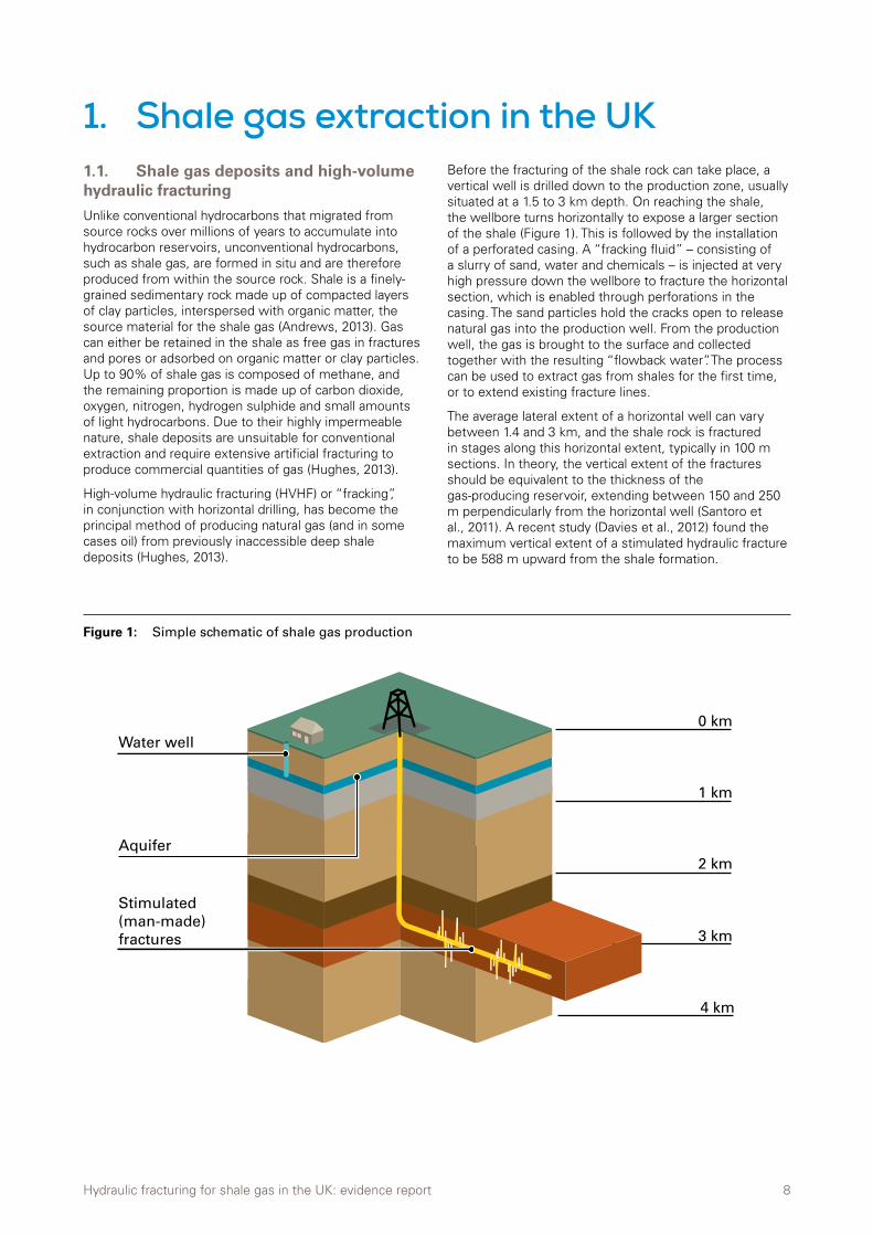
Figure 1: Simple schematic of shale gas production
1.1. Shale gas deposits and high-volume hydraulic fracturing
Unlike conventional hydrocarbons that migrated from source rocks over millions of years to accumulate into hydrocarbon reservoirs, unconventional hydrocarbons, such as shale gas, are formed in situ and are therefore produced from within the source rock. Shale is a finely-grained sedimentary rock made up of compacted layers of clay particles, interspersed with organic matter, the source material for the shale gas (Andrews, 2013). Gas can either be retained in the shale as free gas in fractures and pores or adsorbed on organic matter or clay particles. Up to 90% of shale gas is composed of methane, and the remaining proportion is made up of carbon dioxide, oxygen, nitrogen, hydrogen sulphide and small amounts of light hydrocarbons. Due to their highly impermeable nature, shale deposits are unsuitable for conventional extraction and require extensive artificial fracturing to produce commercial quantities of gas (Hughes, 2013).
High-volume hydraulic fracturing (HVHF) or “fracking”, in conjunction with horizontal drilling, has become the principal method of producing natural gas (and in some cases oil) from previously inaccessible deep shale deposits (Hughes, 2013).
Before the fracturing of the shale rock can take place, a vertical well is drilled down to the production zone, usually situated at a 1.5 to 3 km depth. On reaching the shale, the wellbore turns horizontally to expose a larger section of the shale (Figure 1). This is followed by the installation of a perforated casing. A “fracking fluid” – consisting of a slurry of sand, water and chemicals – is injected at very high pressure down the wellbore to fracture the horizontal section, which is enabled through perforations in the casing. The sand particles hold the cracks open to release natural gas into the production well. From the production well, the gas is brought to the surface and collected together with the resulting “flowback water”. The process can be used to extract gas from shales for the first time, or to extend existing fracture lines.
The average lateral extent of a horizontal well can vary between 1.4 and 3 km, and the shale rock is fractured in stages along this horizontal extent, typically in 100 m sections. In theory, the vertical extent of the fractures should be equivalent to the thickness of the gas-producing reservoir, extending between 150 and 250 m perpendicularly from the horizontal well (Santoro et al., 2011). A recent study (Davies et al., 2012) found the maximum vertical extent of a stimulated hydraulic fracture to be 588 m upward from the shale formation.
3 km
2 km
Stimulated (man-made) fractures
Water well
Aquifer
0 km
1 km
4 km
Hydraulic fracturing for shale gas in the UK: evidence report 9
1.2. Shale reserves, licensing and planning in the UK
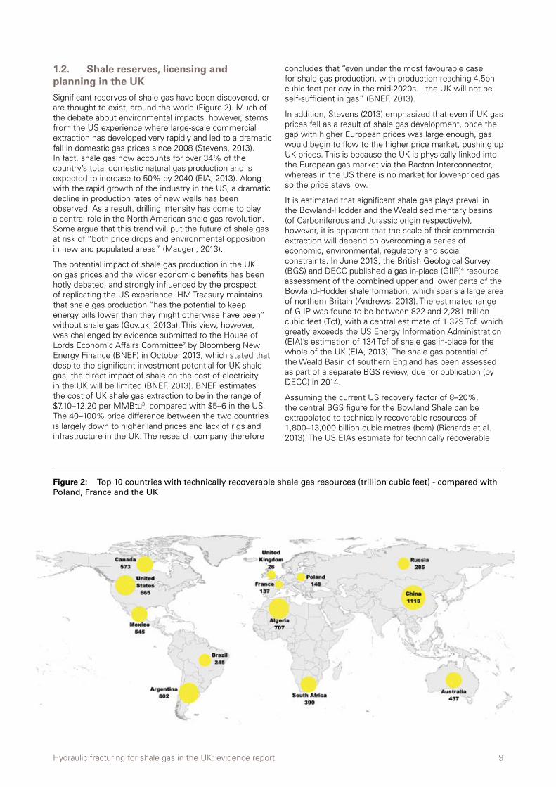
Significant reserves of shale gas have been discovered, or are thought to exist, around the world (Figure 2). Much of the debate about environmental impacts, however, stems from the US experience where large-scale commercial extraction has developed very rapidly and led to a dramatic fall in domestic gas prices since 2008 (Stevens, 2013). In fact, shale gas now accounts for over 34% of the country’s total domestic natural gas production and is expected to increase to 50% by 2040 (EIA, 2013). Along with the rapid growth of the industry in the US, a dramatic decline in production rates of new wells has been observed. As a result, drilling intensity has come to play a central role in the North American shale gas revolution. Some argue that this trend will put the future of shale gas at risk of “both price drops and environmental opposition in new and populated areas” (Maugeri, 2013).
The potential impact of shale gas production in the UK on gas prices and the wider economic benefits has been hotly debated, and strongly influenced by the prospect of replicating the US experience. HM Treasury maintains that shale gas production “has the potential to keep energy bills lower than they might otherwise have been” without shale gas (Gov.uk, 2013a). This view, however, was challenged by evidence submitted to the House of Lords Economic Affairs Committee2 by Bloomberg New Energy Finance (BNEF) in October 2013, which stated that despite the significant investment potential for UK shale gas, the direct impact of shale on the cost of electricity in the UK will be limited (BNEF, 2013). BNEF estimates the cost of UK shale gas extraction to be in the range of $7.10–12.20 per MMBtu3, compared with $5–6 in the US. The 40–100% price difference between the two countries is largely down to higher land prices and lack of rigs and infrastructure in the UK. The research company therefore
concludes that “even under the most favourable case for shale gas production, with production reaching 4.5bn cubic feet per day in the mid-2020s... the UK will not be self-sufficient in gas” (BNEF, 2013).
In addition, Stevens (2013) emphasized that even if UK gas prices fell as a result of shale gas development, once the gap with higher European prices was large enough, gas would begin to flow to the higher price market, pushing up UK prices. This is because the UK is physically linked into the European gas market via the Bacton Interconnector, whereas in the US there is no market for lower-priced gas so the price stays low.
It is estimated that significant shale gas plays prevail in the Bowland-Hodder and the Weald sedimentary basins (of Carboniferous and Jurassic origin respectively), however, it is apparent that the scale of their commercial extraction will depend on overcoming a series of economic, environmental, regulatory and social constraints. In June 2013, the British Geological Survey (BGS) and DECC published a gas in-place (GIIP)4 resource assessment of the combined upper and lower parts of the Bowland-Hodder shale formation, which spans a large area of northern Britain (Andrews, 2013). The estimated range of GIIP was found to be between 822 and 2,281 trillion cubic feet (Tcf), with a central estimate of 1,329 Tcf, which greatly exceeds the US Energy Information Administration (EIA)’s estimation of 134 Tcf of shale gas in-place for the whole of the UK (EIA, 2013). The shale gas potential of the Weald Basin of southern England has been assessed as part of a separate BGS review, due for publication (by DECC) in 2014.
Assuming the current US recovery factor of 8–20%, the central BGS figure for the Bowland Shale can be extrapolated to technically recoverable resources of 1,800–13,000 billion cubic metres (bcm) (Richards et al. 2013). The US EIA’s estimate for technically recoverable
Figure 2: Top 10 countries with technically recoverable shale gas resources (trillion cubic feet) - compared with Poland, France and the UK
Hydraulic fracturing for shale gas in the UK: evidence report 10
shale gas resources in the UK is only a fraction of the figure estimated by Richards et al. (2013) at 26 Tcf, which equals 736 bcm (EIA, 2013).
All shale gas in the UK is owned by the state, and the Government has the right to grant Petroleum Exploration and Development Licence (PEDL) licences under the Petroleum Act 1988 to explore, drill and extract hydrocarbons. As the responsible authority for the licensing of drilling areas, the Department of Energy and Climate Change (DECC) states that “[onshore production licenses] do not confer any exemption from other legal/regulatory requirements such as any need to gain access rights from landowners, health and safety regulations or planning permission from relevant local authorities” (Gov.uk, 2013b). The award of licences is discretionary and they are issued in rounds, which grant exclusivity to operators in particular locations.
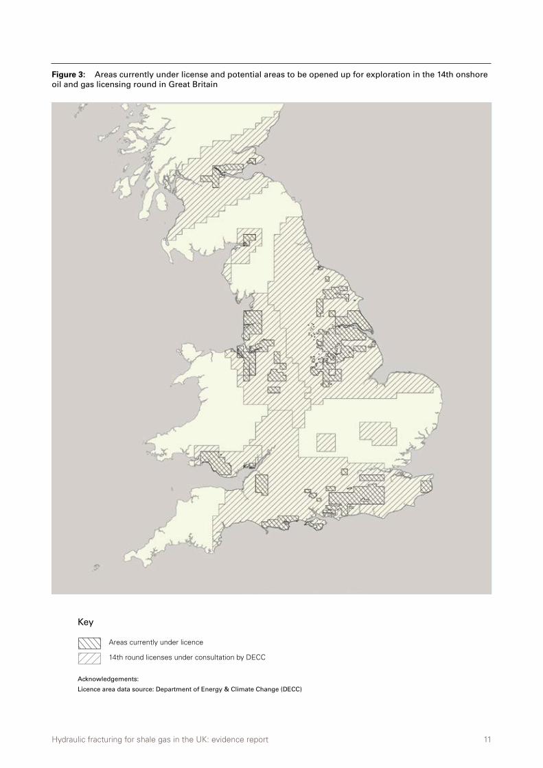
Licences have been granted through a series of onshore licensing rounds, with the 14th round expected to be launched in mid-2014 (Figure 3)5. Although a number of areas have been licensed for drilling under these rounds, the DECC data and licensing process make no distinction
between conventional and unconventional oil and gas extraction. As such, it is impossible to determine which of the licensed areas are being targeted for shale gas rather than conventional hydrocarbons. However, the size of the area licensed under the 14th round may be a good indicator of the growing interest in the onshore exploration of unconventional hydrocarbons.
Almost all exploratory activities in the UK have so far occurred in the Bowland shales of Lancashire – in the northwest of England – where Cuadrilla Resources Ltd. (Cuadrilla) began test drilling for shale gas in August 2010. The first of such sites was “Preese Hall”, near Weeton where HVHF activity resulted in a series of seismic events in April and May 2011, leading to a UK-wide moratorium that has now been lifted. Cuadrilla has carried out test drilling at two other sites, namely Grange Hill, near Singleton and Becconsall at Banks, however “Preese Hall” remains the only hydraulically fractured shale gas well at present. Exploratory activities for shale gas in other parts of the UK, including the southeast of England, southern Wales and the southwest of Northern Ireland, are predominantly at the planning stage.
2 In July 2013, the House of Lords Economic Affairs Committee launched an inquiry into the economic impact of shale gas and oil on UK Energy Policy (UK Parliament, 2014). BNEF’s evidence was submitted to the Select Committee in response to this inquiry.
3 Natural gas is measured in MMBtu, which is equal to one million British Thermal Units (BTU)
4 GIIP refers to an estimate for the overall volume of gas in the shales; it does not reflect the volume of technically recoverable shale gas reserves.
5 Please note license blocks are not shown in Northern Ireland (NI) where petroleum licenses are granted by the Department of Enterprise, Trade and Investment (DETI) through a separate licensing process (ie, an open-door system) to that adopted by the DECC, which issues PEDL licenses for the rest of the UK via a series of licensing rounds. Hence license areas in NI have been excluded from the report.
How many wells?The estimate of up to 120 well pads referred to in this report is taken from DECC’s Strategic Environmental Assessment of the 14th onshore oil and gas licensing round for Great Britain. It applies only to the commercial extraction activity associated with this round and is in addition to previous and future rounds, which are expected to be held every couple of years. Estimates of total well pad numbers for commercial extraction in the UK vary depending on assumptions around the number of wells
that will be associated with individual pads. Most recently, Professor Andrew Aplin (2014) of Durham University estimated that the Upper Bowland Basin alone could require up to 33,000 wells. Based on the industry practices in the US, this would mean 5,500 individual well pads; however the UK Government has argued that the UK industry is likely to concentrate well activity around a smaller number of sites.
Hydraulic fracturing for shale gas in the UK: evidence report 11
Figure 3: Areas currently under license and potential areas to be opened up for exploration in the 14th onshore oil and gas licensing round in Great Britain
Key
Areas currently under licence
14th round licenses under consultation by DECC
Acknowledgements:
Licence area data source: Department of Energy & Climate Change (DECC)
Key:
Acknowledgements:
0 6030 Km
E1:3,600,000Scale on A4 paperAreas currently under licence 14th roundlicences under consultation by DECC (GB)
Areas currently under licence and 14th round licences underconsultation by DECC (GB)
Licence area data source: Department of Energy & Climate Change (DECC)
Key:
Acknowledgements:
0 6030 Km
E1:3,600,000Scale on A4 paperAreas currently under licence 14th roundlicences under consultation by DECC (GB)
Areas currently under licence and 14th round licences underconsultation by DECC (GB)
Licence area data source: Department of Energy & Climate Change (DECC)
Hydraulic fracturing for shale gas in the UK: evidence report 12
Many of the risks and challenges associated with shale gas extraction are comparable to conventional hydrocarbon operations, and these are already covered by robust regulation in the UK. New regulation is, however, needed to reflect the environmental risks specific to shale gas exploration and to ensure these are effectively managed, in particular, as exploratory activities move to large-scale commercial production. By means of a comprehensive literature review, this report identified three main areas of potential risk typically associated with shale gas extraction, namely:
• Groundwater and surface water contamination
• Water use and disposal
• Species disturbance, and habitat loss and fragmentation.
The report also addresses the environmental impact of carbon emissions resulting from the end use of shale gas; however detailed analysis of such impacts is outside the scope of this report. Moreover, a detailed study of local greenhouse gas emissions associated with shale gas exploration and production has already been conducted by
MacKay and Stone (2013) for DECC, therefore we chose not to focus on this issue.
The potential for environmental impacts depends on many variables. These are most notably the geology of the area being drilled, the depth of well, the operational practices, chemicals and equipment being used, and the proximity of groundwater, surface water and sensitive habitats and species.
Our ability to quantify such risks has been limited by the absence of evidence and the variability in practices across different parts of the US – the country with the most mature extractive industry. Different US states have applied different regulations to shale gas extraction, some of which would clearly be unacceptable in the UK, eg disposal of flowback water via evaporation ponds or underground injection. The industry’s lack of transparency over practices, such as the chemicals used in the HVHF process, and the use of non-disclosure agreements with landowners have complicated the risk characterisation and assessment process. This confusion has made it very difficult to differentiate fact from fiction in the ongoing debate and, ultimately, to establish industry best practice.
2. Types of environmental risks and their management
Hydraulic fracturing for shale gas in the UK: evidence report 13
3. Impacts on the water environment Whilst there are clear risks posed to surface water and groundwater by shale gas exploration and production (Figure 4), it is important to draw attention to the paucity of studies and data available in the peer-reviewed scientific literature. In fact, whilst much has been written about the impact of the HVHF process on water quality or resources, the majority of this writing is either industry or advocacy reports that have not been peer-reviewed (Cooley and Donnelly, 2012).
A number of academic as well as government-led studies, however, are currently underway to help fill this knowledge gap and provide a stronger scientific evidence base on the main water-related impacts. Amongst these is a comprehensive study to examine the potential impacts of each stage of the HVHF lifecycle on drinking water resources, currently in development by the US Environmental Protection Agency (EPA). The draft report will be available for public comment and peer review in 2014.
3.1. Groundwater vulnerability
The contamination of groundwater aquifers, by methane or chemicals in the fracturing fluid, has become among the most contentious issues surrounding the global shale gas industry (Healy, 2012). There has been a lot of anecdotal evidence of pollution incidents attributed to the extraction of shale gas by means of HVHF in the US. However, relatively few scientific investigations have been conducted to identify the causes, frequency and magnitude of such groundwater contamination incidents in the major US hydrocarbon-producing states.
There are two potential pathways that give rise to
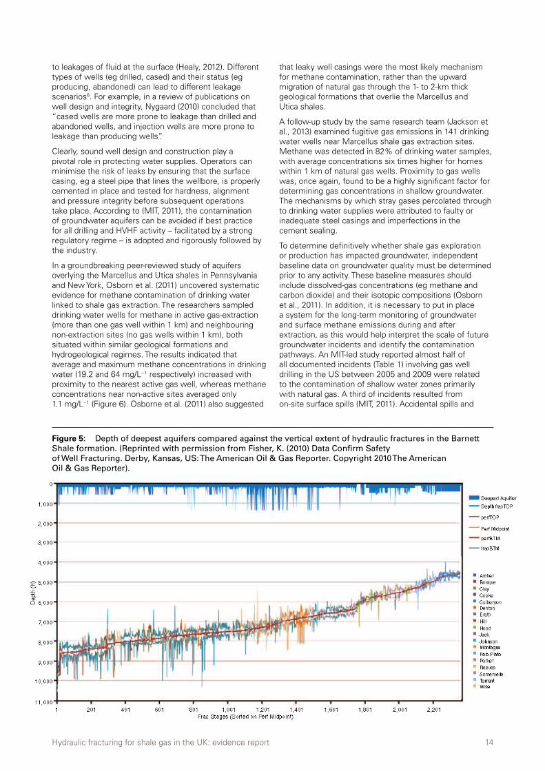
groundwater contamination in the subsurface. Firstly, it has been suggested that contaminants (from the fracking fluid) may percolate upwards through the fractured formation into the overlying shallow aquifer. It is important to note that most aquifers used for drinking water supply in the UK are found within the first 300 m under the surface whereas HVHF operations are typically carried out at a minimum depth of 2 km. Figure 5 illustrates the distance between the deepest aquifers and the perpendicular extent of hydraulic fractures in the Barnett Shale formation. It shows that in all cases the highest growth of the fractures remains isolated from the groundwater aquifers by thousands of feet of formation.
Recent analysis of microseismic measurements from several thousand HVHF operations in the US indicates that the probability of a stimulated fracture extending vertically more than 350 m is around 1% (Davies et al., 2012), with very few fractures propagating past 500 m. To help avoid the unintentional penetration of shallower rock strata, the study recommends for a minimum vertical separation to be maintained between the shale gas reservoir and the groundwater aquifers. However, the authors provide no indication of what this safe distance should be. Moreover, due to the unique nature of each shale gas play, it is essential to fully evaluate on a case-by-case basis the risks of hydraulic connectivity between the shale formation and overlying aquifers before HVHF operations begin.
Secondly, leakages of fracking chemicals or methane may occur from imperfectly sealed shale gas wells that pass through aquifers. In fact, most peer-reviewed studies that document cases of groundwater contamination associated with shale gas extraction are linked to poor well design or
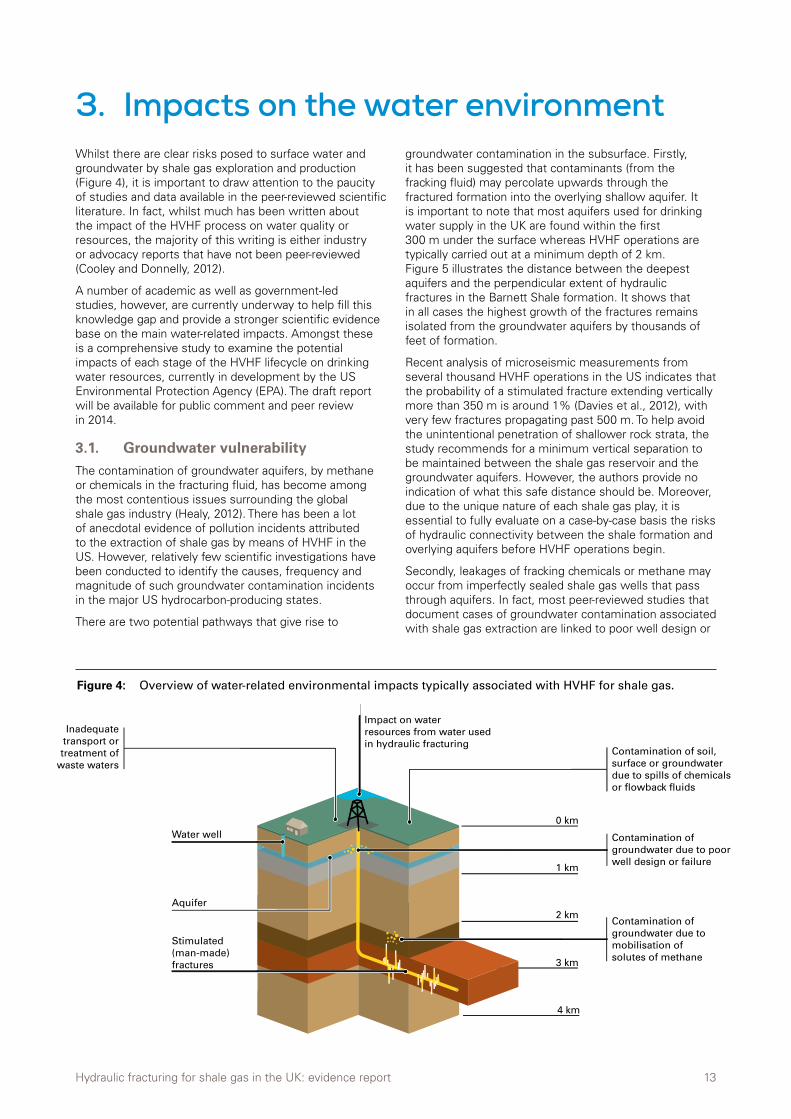
Figure 4: Overview of water-related environmental impacts typically associated with HVHF for shale gas.
3 km
2 km
Stimulated (man-made) fractures
Water well
Aquifer
0 km
1 km
4 km
Impact on water resources from water used in hydraulic fracturing
Contamination of groundwater due to poor well design or failure
Inadequate transport or treatment of
waste waters
Contamination of groundwater due to mobilisation of solutes of methane
Contamination of soil, surface or groundwater due to spills of chemicals or flowback fluids
Hydraulic fracturing for shale gas in the UK: evidence report 14
to leakages of fluid at the surface (Healy, 2012). Different types of wells (eg drilled, cased) and their status (eg producing, abandoned) can lead to different leakage scenarios6. For example, in a review of publications on well design and integrity, Nygaard (2010) concluded that “cased wells are more prone to leakage than drilled and abandoned wells, and injection wells are more prone to leakage than producing wells”.
Clearly, sound well design and construction play a pivotal role in protecting water supplies. Operators can minimise the risk of leaks by ensuring that the surface casing, eg a steel pipe that lines the wellbore, is properly cemented in place and tested for hardness, alignment and pressure integrity before subsequent operations take place. According to (MIT, 2011), the contamination of groundwater aquifers can be avoided if best practice for all drilling and HVHF activity – facilitated by a strong regulatory regime – is adopted and rigorously followed by the industry.
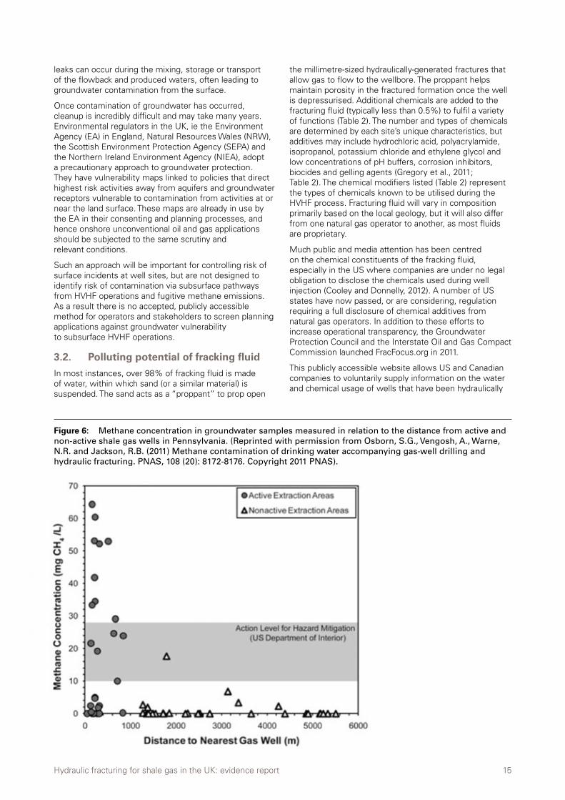
In a groundbreaking peer-reviewed study of aquifers overlying the Marcellus and Utica shales in Pennsylvania and New York, Osborn et al. (2011) uncovered systematic evidence for methane contamination of drinking water linked to shale gas extraction. The researchers sampled drinking water wells for methane in active gas-extraction (more than one gas well within 1 km) and neighbouring non-extraction sites (no gas wells within 1 km), both situated within similar geological formations and hydrogeological regimes. The results indicated that average and maximum methane concentrations in drinking water (19.2 and 64 mg/L−1 respectively) increased with proximity to the nearest active gas well, whereas methane concentrations near non-active sites averaged only 1.1 mg/L−1 (Figure 6). Osborne et al. (2011) also suggested
that leaky well casings were the most likely mechanism for methane contamination, rather than the upward migration of natural gas through the 1- to 2-km thick geological formations that overlie the Marcellus and Utica shales.
A follow-up study by the same research team (Jackson et al., 2013) examined fugitive gas emissions in 141 drinking water wells near Marcellus shale gas extraction sites. Methane was detected in 82% of drinking water samples, with average concentrations six times higher for homes within 1 km of natural gas wells. Proximity to gas wells was, once again, found to be a highly significant factor for determining gas concentrations in shallow groundwater. The mechanisms by which stray gases percolated through to drinking water supplies were attributed to faulty or inadequate steel casings and imperfections in the cement sealing.
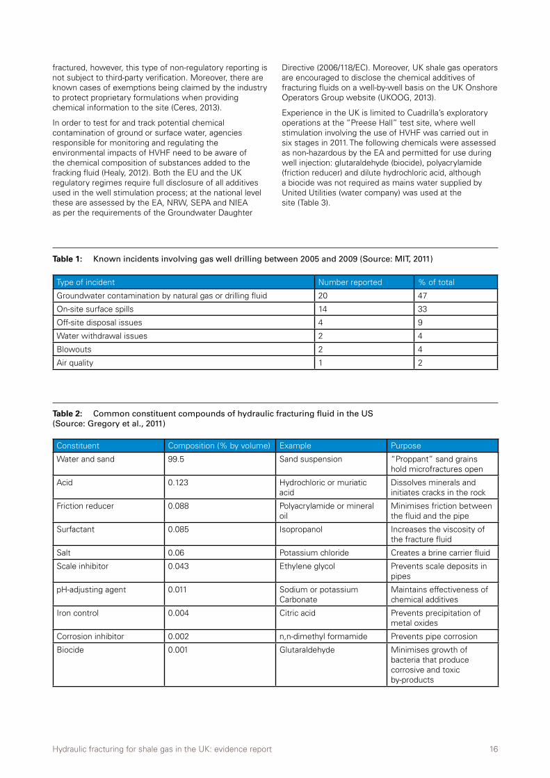
To determine definitively whether shale gas exploration or production has impacted groundwater, independent baseline data on groundwater quality must be determined prior to any activity. These baseline measures should include dissolved-gas concentrations (eg methane and carbon dioxide) and their isotopic compositions (Osborn et al., 2011). In addition, it is necessary to put in place a system for the long-term monitoring of groundwater and surface methane emissions during and after extraction, as this would help interpret the scale of future groundwater incidents and identify the contamination pathways. An MIT-led study reported almost half of all documented incidents (Table 1) involving gas well drilling in the US between 2005 and 2009 were related to the contamination of shallow water zones primarily with natural gas. A third of incidents resulted from on-site surface spills (MIT, 2011). Accidental spills and
Figure 5: Depth of deepest aquifers compared against the vertical extent of hydraulic fractures in the Barnett Shale formation. (Reprinted with permission from Fisher, K. (2010) Data Confirm Safety of Well Fracturing. Derby, Kansas, US: The American Oil & Gas Reporter. Copyright 2010 The American Oil & Gas Reporter).
Hydraulic fracturing for shale gas in the UK: evidence report 15
leaks can occur during the mixing, storage or transport of the flowback and produced waters, often leading to groundwater contamination from the surface.
Once contamination of groundwater has occurred, cleanup is incredibly difficult and may take many years. Environmental regulators in the UK, ie the Environment Agency (EA) in England, Natural Resources Wales (NRW), the Scottish Environment Protection Agency (SEPA) and the Northern Ireland Environment Agency (NIEA), adopt a precautionary approach to groundwater protection. They have vulnerability maps linked to policies that direct highest risk activities away from aquifers and groundwater receptors vulnerable to contamination from activities at or near the land surface. These maps are already in use by the EA in their consenting and planning processes, and hence onshore unconventional oil and gas applications should be subjected to the same scrutiny and relevant conditions.
Such an approach will be important for controlling risk of surface incidents at well sites, but are not designed to identify risk of contamination via subsurface pathways from HVHF operations and fugitive methane emissions. As a result there is no accepted, publicly accessible method for operators and stakeholders to screen planning applications against groundwater vulnerability to subsurface HVHF operations.
3.2. Polluting potential of fracking fluid
In most instances, over 98% of fracking fluid is made of water, within which sand (or a similar material) is suspended. The sand acts as a “proppant” to prop open
the millimetre-sized hydraulically-generated fractures that allow gas to flow to the wellbore. The proppant helps maintain porosity in the fractured formation once the well is depressurised. Additional chemicals are added to the fracturing fluid (typically less than 0.5%) to fulfil a variety of functions (Table 2). The number and types of chemicals are determined by each site’s unique characteristics, but additives may include hydrochloric acid, polyacrylamide, isopropanol, potassium chloride and ethylene glycol and low concentrations of pH buffers, corrosion inhibitors, biocides and gelling agents (Gregory et al., 2011; Table 2). The chemical modifiers listed (Table 2) represent the types of chemicals known to be utilised during the HVHF process. Fracturing fluid will vary in composition primarily based on the local geology, but it will also differ from one natural gas operator to another, as most fluids are proprietary.
Much public and media attention has been centred on the chemical constituents of the fracking fluid, especially in the US where companies are under no legal obligation to disclose the chemicals used during well injection (Cooley and Donnelly, 2012). A number of US states have now passed, or are considering, regulation requiring a full disclosure of chemical additives from natural gas operators. In addition to these efforts to increase operational transparency, the Groundwater Protection Council and the Interstate Oil and Gas Compact Commission launched FracFocus.org in 2011.
This publicly accessible website allows US and Canadian companies to voluntarily supply information on the water and chemical usage of wells that have been hydraulically
Figure 6: Methane concentration in groundwater samples measured in relation to the distance from active and non-active shale gas wells in Pennsylvania. (Reprinted with permission from Osborn, S.G., Vengosh, A., Warne, N.R. and Jackson, R.B. (2011) Methane contamination of drinking water accompanying gas-well drilling and hydraulic fracturing. PNAS, 108 (20): 8172-8176. Copyright 2011 PNAS).
Hydraulic fracturing for shale gas in the UK: evidence report 16
fractured, however, this type of non-regulatory reporting is not subject to third-party verification. Moreover, there are known cases of exemptions being claimed by the industry to protect proprietary formulations when providing chemical information to the site (Ceres, 2013).
In order to test for and track potential chemical contamination of ground or surface water, agencies responsible for monitoring and regulating the environmental impacts of HVHF need to be aware of the chemical composition of substances added to the fracking fluid (Healy, 2012). Both the EU and the UK regulatory regimes require full disclosure of all additives used in the well stimulation process; at the national level these are assessed by the EA, NRW, SEPA and NIEA as per the requirements of the Groundwater Daughter
Directive (2006/118/EC). Moreover, UK shale gas operators are encouraged to disclose the chemical additives of fracturing fluids on a well-by-well basis on the UK Onshore Operators Group website (UKOOG, 2013).
Experience in the UK is limited to Cuadrilla’s exploratory operations at the “Preese Hall” test site, where well stimulation involving the use of HVHF was carried out in six stages in 2011. The following chemicals were assessed as non-hazardous by the EA and permitted for use during well injection: glutaraldehyde (biocide), polyacrylamide (friction reducer) and dilute hydrochloric acid, although a biocide was not required as mains water supplied by United Utilities (water company) was used at the site (Table 3).
Type of incident Number reported % of total
Groundwater contamination by natural gas or drilling fluid 20 47
On-site surface spills 14 33
Off-site disposal issues 4 9
Water withdrawal issues 2 4
Blowouts 2 4
Air quality 1 2
Table 1: Known incidents involving gas well drilling between 2005 and 2009 (Source: MIT, 2011)
Constituent Composition (% by volume) Example Purpose
Water and sand 99.5 Sand suspension “Proppant” sand grains hold microfractures open
Acid 0.123 Hydrochloric or muriatic acid
Dissolves minerals and initiates cracks in the rock
Friction reducer 0.088 Polyacrylamide or mineral oil
Minimises friction between the fluid and the pipe
Surfactant 0.085 Isopropanol Increases the viscosity of the fracture fluid
Salt 0.06 Potassium chloride Creates a brine carrier fluid
Scale inhibitor 0.043 Ethylene glycol Prevents scale deposits in pipes
pH-adjusting agent 0.011 Sodium or potassium Carbonate
Maintains effectiveness of chemical additives
Iron control 0.004 Citric acid Prevents precipitation of metal oxides
Corrosion inhibitor 0.002 n,n-dimethyl formamide Prevents pipe corrosion
Biocide 0.001 Glutaraldehyde Minimises growth of bacteria that produce corrosive and toxic by-products
Table 2: Common constituent compounds of hydraulic fracturing fluid in the US (Source: Gregory et al., 2011)
Hydraulic fracturing for shale gas in the UK: evidence report 17
3.3. Water usage
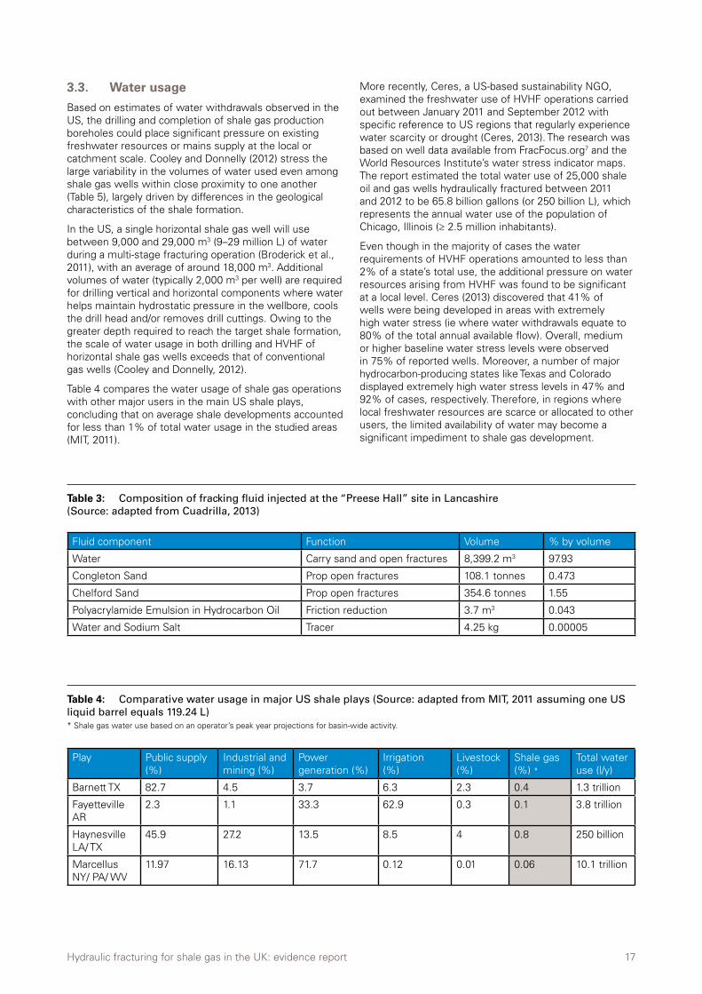
Based on estimates of water withdrawals observed in the US, the drilling and completion of shale gas production boreholes could place significant pressure on existing freshwater resources or mains supply at the local or catchment scale. Cooley and Donnelly (2012) stress the large variability in the volumes of water used even among shale gas wells within close proximity to one another (Table 5), largely driven by differences in the geological characteristics of the shale formation.
In the US, a single horizontal shale gas well will use between 9,000 and 29,000 m3 (9–29 million L) of water during a multi-stage fracturing operation (Broderick et al., 2011), with an average of around 18,000 m3. Additional volumes of water (typically 2,000 m3 per well) are required for drilling vertical and horizontal components where water helps maintain hydrostatic pressure in the wellbore, cools the drill head and/or removes drill cuttings. Owing to the greater depth required to reach the target shale formation, the scale of water usage in both drilling and HVHF of horizontal shale gas wells exceeds that of conventional gas wells (Cooley and Donnelly, 2012).
Table 4 compares the water usage of shale gas operations with other major users in the main US shale plays, concluding that on average shale developments accounted for less than 1% of total water usage in the studied areas (MIT, 2011).
More recently, Ceres, a US-based sustainability NGO, examined the freshwater use of HVHF operations carried out between January 2011 and September 2012 with specific reference to US regions that regularly experience water scarcity or drought (Ceres, 2013). The research was based on well data available from FracFocus.org7 and the World Resources Institute’s water stress indicator maps. The report estimated the total water use of 25,000 shale oil and gas wells hydraulically fractured between 2011 and 2012 to be 65.8 billion gallons (or 250 billion L), which represents the annual water use of the population of Chicago, Illinois (≥ 2.5 million inhabitants).
Even though in the majority of cases the water requirements of HVHF operations amounted to less than 2% of a state’s total use, the additional pressure on water resources arising from HVHF was found to be significant at a local level. Ceres (2013) discovered that 41% of wells were being developed in areas with extremely high water stress (ie where water withdrawals equate to 80% of the total annual available flow). Overall, medium or higher baseline water stress levels were observed in 75% of reported wells. Moreover, a number of major hydrocarbon-producing states like Texas and Colorado displayed extremely high water stress levels in 47% and 92% of cases, respectively. Therefore, in regions where local freshwater resources are scarce or allocated to other users, the limited availability of water may become a significant impediment to shale gas development.
Fluid component Function Volume % by volume
Water Carry sand and open fractures 8,399.2 m3 97.93
Congleton Sand Prop open fractures 108.1 tonnes 0.473
Chelford Sand Prop open fractures 354.6 tonnes 1.55
Polyacrylamide Emulsion in Hydrocarbon Oil Friction reduction 3.7 m3 0.043
Water and Sodium Salt Tracer 4.25 kg 0.00005
Table 3: Composition of fracking fluid injected at the “Preese Hall” site in Lancashire (Source: adapted from Cuadrilla, 2013)
Play Public supply (%)
Industrial and mining (%)
Power generation (%)
Irrigation (%)
Livestock (%)
Shale gas (%) *
Total water use (l/y)
Barnett TX 82.7 4.5 3.7 6.3 2.3 0.4 1.3 trillion
Fayetteville AR
2.3 1.1 33.3 62.9 0.3 0.1 3.8 trillion
Haynesville LA/ TX
45.9 27.2 13.5 8.5 4 0.8 250 billion
Marcellus NY/ PA/ WV
11.97 16.13 71.7 0.12 0.01 0.06 10.1 trillion
Table 4: Comparative water usage in major US shale plays (Source: adapted from MIT, 2011 assuming one US liquid barrel equals 119.24 L) * Shale gas water use based on an operator’s peak year projections for basin-wide activity.
Hydraulic fracturing for shale gas in the UK: evidence report 18
In the UK, abstracting freshwater for shale gas extraction is also likely to result in additional stress, “given that water resources in many parts of the [country] are already under pressure” (Broderick et al., 2011). For example, the annual production of 9 bcm8 of shale gas would necessitate 1.25 to 1.65 million m3 of water a year (based on Cuadrilla’s water usage at “Preese Hall”). To maintain this level of production for a period of two decades would therefore require around 2,500–3,000 horizontal wells and some 25 to 33 million m3 of water (Broderick et al. 2011). Relatively small additional drains on potentially stressed water resources at the local level can become much more pronounced through the additive effects of multiple wells in a region and poor phasing of HVHF.
The Royal Society’s report (RS/RAENG, 2012) indicates that the water requirements for the shale gas industry can be managed sustainably since abstraction in the UK is a regulated activity. In England, for instance, the EA is responsible for assessing existing abstraction levels and licenses before granting a license to abstract. At the “Preese Hall” well, Cuadrilla used approximately 1,400 m3 of freshwater for each of the six stages of HVHF, adding up to a total of 8,400 m3 (8.4 mil L), which places the water use of this well at the lower to medium end of figures reported from operations in Texas (Table 5). However, it is important to note that this type of water use is not continuous. Peaks in demand will be expected at various stages of the HVHF process and during the well’s operating life. As a result, careful timing of operations and good communication with water companies and the relevant environment regulator (EA, NRW, SEPA or NIEA) will be vital in reducing stress on natural or public water supplies.
In an effort to reduce the impact on local water resources, particularly in areas where hydraulic fracturing is new or water is relatively scarce, recycled or brackish water is increasingly being considered for HVHF operations (Ceres, 2013). Recycling is seen by the industry as both an economic and environmental win, since it decreases the need for long-range trucking of water to the well pad and subsequent wastewaters to off-site disposal facilities. However, in many cases flowback water will have to be treated prior to reuse, possibly using nanofiltration and reverse osmosis systems to clean and concentrate high salinity produced waters (RS/RAENG, 2012). Such
treatment adds cost and has energy implications, adding to the carbon footprint; however, recycling might be important in mitigating impacts in water stressed areas.
Waterless fracturing by means of gels, carbon dioxide and nitrogen gas foams is also becoming a possible alternative to fracking fluid (King, 2010), however there are no public proposals to pursue this technology in the UK.
3.3.1. Analysis of water resource impacts in England and Wales9
According to the European Environment Agency, the UK is one of nine EU Member States that is water-stressed (EEA, 2008). The degree of water stress is variable across the UK. In fact, the majority of southeast and eastern England is presently under moderate to serious water stress, as stated in the 2013 classifications of water stress in individual water company areas (EA and NRW, 2013). By contrast, the utilities serving northern England are in areas of moderate to low water stress, including United Utilities, which supplied Cuadrilla with mains water for the drilling and hydraulic fracturing phases of their Lancashire exploration well site at “Preese Hall”.
In addition to regional water shortage pressures, total water demand is expected to rise steadily over the next decade. The Environment Agency (England) estimates that by 2020 demand could be roughly 5% higher compared to today. Moreover, the Water Resources Strategy for England and Wales shows that by 2050 changing rainfall patterns induced by climate change could lead to a 15% drop in total annual average river flows, and that long-term aquifer recharge is likely to decrease by 3–9% by 2025 (EA, 2009). Consequently, rising water demand coupled with reduced annual surface water and groundwater flows, could lead to more frequent and pronounced drought events in the upcoming decades, such as those experienced in 2011 and early 2012, both of which attest to the fact that the UK’s water resources are not unlimited.
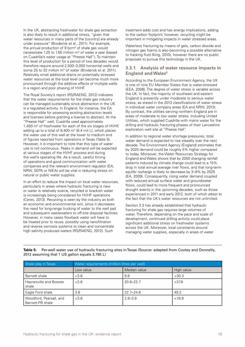
Section 3.3 has already established that hydraulic fracturing for shale gas requires large volumes of water. Therefore, depending on the pace and scale of development, continued drilling activity could place significant additional stress on freshwater systems across the UK. Moreover, local constraints around managing water supplies, especially in areas of water
Shale play in Texas Water requirements (million litres per well)
Low value Median value High value
Barnett shale <3.8 9.8 >30.3
Haynesville and Bossier shale
<3.8 20.8–22.7 >37.8
Eagle Ford shale 3.8 22.7–24.6 49.2
Woodford, Pearsall, and Barnett-PB shale
<3.8 2.8–3.8 <18.9
Table 5: Per-well water use of hydraulic fracturing sites in Texas (Source: adapted from Cooley and Donnelly, 2012 assuming that 1 US gallon equals 3.785 L)
Hydraulic fracturing for shale gas in the UK: evidence report 19
stress or at times of prolonged drought, may arise as a result of fluctuating water needs of the shale gas industry throughout the year. Therefore, the phasing of onsite activities to reduce peak demand and avoid times of water scarcity is an essential consideration for the industry.
A number of organisations and public bodies, such as DECC, the EA, Institute of Directors and the Tyndall Centre for Climate Change Research, have attempted to estimate the potential impacts of shale gas development in the UK on national water demand and water resource availability. According to DECC, total water consumption associated with HVHF over a 20-year period could reach 57.6–144 million m3 under the high activity scenario (ie annual water use of 9 million m3)10, representing “substantially less than 1% of total UK annual non domestic mains water usage” (AMEC, 2013). The AMEC report also notes that “the potential impacts that this [level of water use] could have on, for example, water resource availability, aquatic habitats and ecosystems and water quality [are] ... more uncertain” (AMEC, 2013). The Tyndall Centre for Climate Change Research (Broderick et al., 2011), for instance, reported a 0.6%11 increase in water abstraction needed to support a shale gas industry that delivers 10% of UK gas consumption (ie 9 bcm per year).
Where natural gas extraction results in over-abstraction of surface- or ground-water supplies, there is potential for conflict with other human uses (eg agricultural and domestic use) and for negative ecological impacts, such as a designated species or habitat affected by reduced in-stream flows. The extent of such conflicts and environmental impacts depends on existing water
demands and the availability of water to meet those demands.
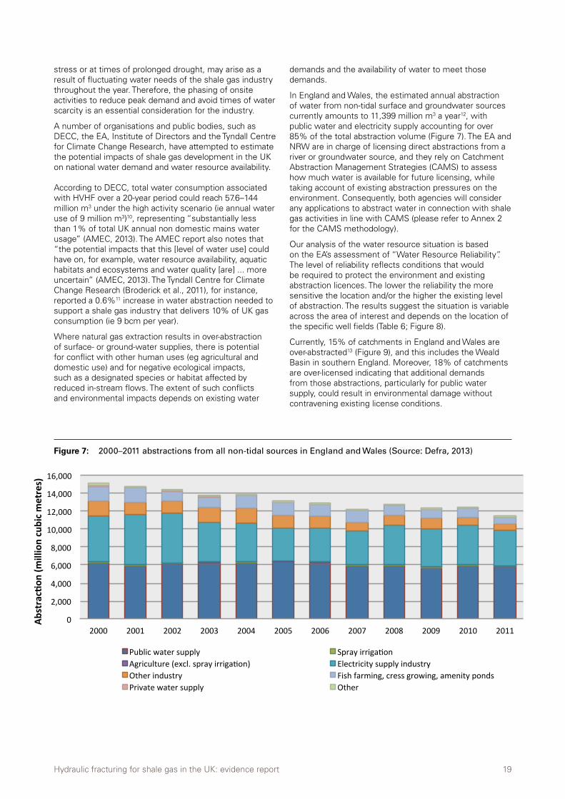
In England and Wales, the estimated annual abstraction of water from non-tidal surface and groundwater sources currently amounts to 11,399 million m3 a year12, with public water and electricity supply accounting for over 85% of the total abstraction volume (Figure 7). The EA and NRW are in charge of licensing direct abstractions from a river or groundwater source, and they rely on Catchment Abstraction Management Strategies (CAMS) to assess how much water is available for future licensing, while taking account of existing abstraction pressures on the environment. Consequently, both agencies will consider any applications to abstract water in connection with shale gas activities in line with CAMS (please refer to Annex 2 for the CAMS methodology).
Our analysis of the water resource situation is based on the EA’s assessment of “Water Resource Reliability”. The level of reliability reflects conditions that would be required to protect the environment and existing abstraction licences. The lower the reliability the more sensitive the location and/or the higher the existing level of abstraction. The results suggest the situation is variable across the area of interest and depends on the location of the specific well fields (Table 6; Figure 8).
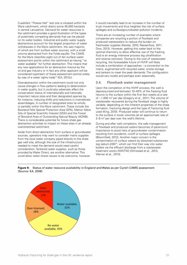
Currently, 15% of catchments in England and Wales are over-abstracted13 (Figure 9), and this includes the Weald Basin in southern England. Moreover, 18% of catchments are over-licensed indicating that additional demands from those abstractions, particularly for public water supply, could result in environmental damage without contravening existing license conditions.
Figure 7: 2000–2011 abstractions from all non-tidal sources in England and Wales (Source: Defra, 2013)
0
2,000
4,000
6,000
8,000
10,000
12,000
14,000
16,000
2000 2001 2002 2003 2004 2005 2006 2007 2008 2009 2010 2011
Abstrac(on
(million cubic metres)
Public water supply Spray irriga=on Agriculture (excl. spray irriga=on) Electricity supply industry Other industry Fish farming, cress growing, amenity ponds Private water supply Other

Hydraulic fracturing for shale gas in the UK: evidence report 20
Key
Areas currently under licence
14th round licenses under consultation by DECC (GB)
Acknowledgements:
Licence area data source: Department of Energy & Climate Change (DECC). Water resource reliability are based on digital spatial data licensed from the Centre of Ecology and Hydrology, © CEH supplied by the Environment Agency
Key:
Acknowledgements:
0 6030 Km
E1:3,600,000Scale on A4 paperAreas currently under licence 14th roundlicences under consultation by DECC (GB)
Areas currently under licence and 14th round licences underconsultation by DECC (GB)
Licence area data source: Department of Energy & Climate Change (DECC)
Key:
Acknowledgements:
0 6030 Km
E1:3,600,000Scale on A4 paperAreas currently under licence 14th roundlicences under consultation by DECC (GB)
Areas currently under licence and 14th round licences underconsultation by DECC (GB)
Licence area data source: Department of Energy & Climate Change (DECC)
Resource availability (% of the time)
less than 30%
at least 30%
at least 50%
at least 70%
at least 95%
Figure 8: Water resource reliability (England and Wales) intersected with areas currently under license and potential areas to be opened up for exploration in the 14th onshore oil and gas licensing round in Great Britain
Hydraulic fracturing for shale gas in the UK: evidence report 21
Cuadrilla’s “Preese Hall” test site is situated within the Wyre catchment, which drains some 45,000 hectares in central Lancashire. Demand for water resources in the catchment provides a good illustration of the types of potentially competing demands that can be placed on its water bodies. Industrial and public water supply abstractions account for the largest proportion of water withdrawals in the Wyre catchment, the vast majority of which are from surface water sources, with a small volume abstracted from the Fylde aquifer. The CAMS for the Wyre classifies eight out of ten surface water assessment points within the catchment as having “no water available” for further abstraction. This means that any new applications for an abstraction licence by the oil and gas industry or in fact any other applicant will be considered (upstream of these assessment points) solely by way of a water rights trade14 (EA, 2013c).
Over-abstraction within the catchment could not only cause changes in flow patterns leading to deterioration in water quality, but it could also adversely affect the conservation status of internationally and nationally important nature sites and their designated species by, for instance, inducing shifts and reductions in invertebrate assemblages. A number of designated sites lie wholly or partially within the Wyre catchment. These include the Bowland Fells Special Protection Area (SPA), Marton Mere Site of Special Scientific Interest (SSSI) and the Forest of Bowland Area of Outstanding Natural Beauty (AONB). There is considerable potential for future shale gas abstraction activities to impact on these sites in an already overstretched catchment.
Aside from direct abstraction from surface or groundwater sources, operators may want to consider mains supplies from the local water company piped directly to the shale gas well site, although the size of the infrastructure needed to meet the demand would need careful consideration. Tankered water supplies, such as those provided by Water Direct, are another alternative. This could allow water stress issues to be overcome, however
it would inevitably lead to an increase in the number of truck movements and thus heighten the risk of surface spillages and surface/groundwater pollution incidents.
There are an increasing number of examples where companies are recycling a portion of flowback and produced wastewaters to reduce the burden on freshwater supplies (Keister, 2010; Rassenfoss, 2011; Dow, 2013). However, getting this water back to the optimal chemistry to allow effective use of the fracking fluid is an energy intensive process (eg ultrafiltration and reverse osmosis). Owing to the cost of wastewater recycling, the foreseeable future of HVHF will likely include a combination of approaches – a connection to the mains, augmented with recycled water, onsite storage and tankers to meet the peak demands. The configuration would vary locally and perhaps even seasonally.
3.4. Flowback water management
Upon the completion of the HVHF process, the well is depressurised and between 10–40% of the fracking fluid returns to the surface within the first few weeks at a rate of ~1,000 m3 per day (Gregory et al., 2011). The volume of wastewater recovered during the flowback stage is highly variable, depending on the inherent properties of the shale formation, fracturing design and the type of fracturing fluid used (King, 2010). Produced water will continue to return to the surface in lower volumes (at an approximate rate of 2–8 m3 per day) over the well’s lifetime.
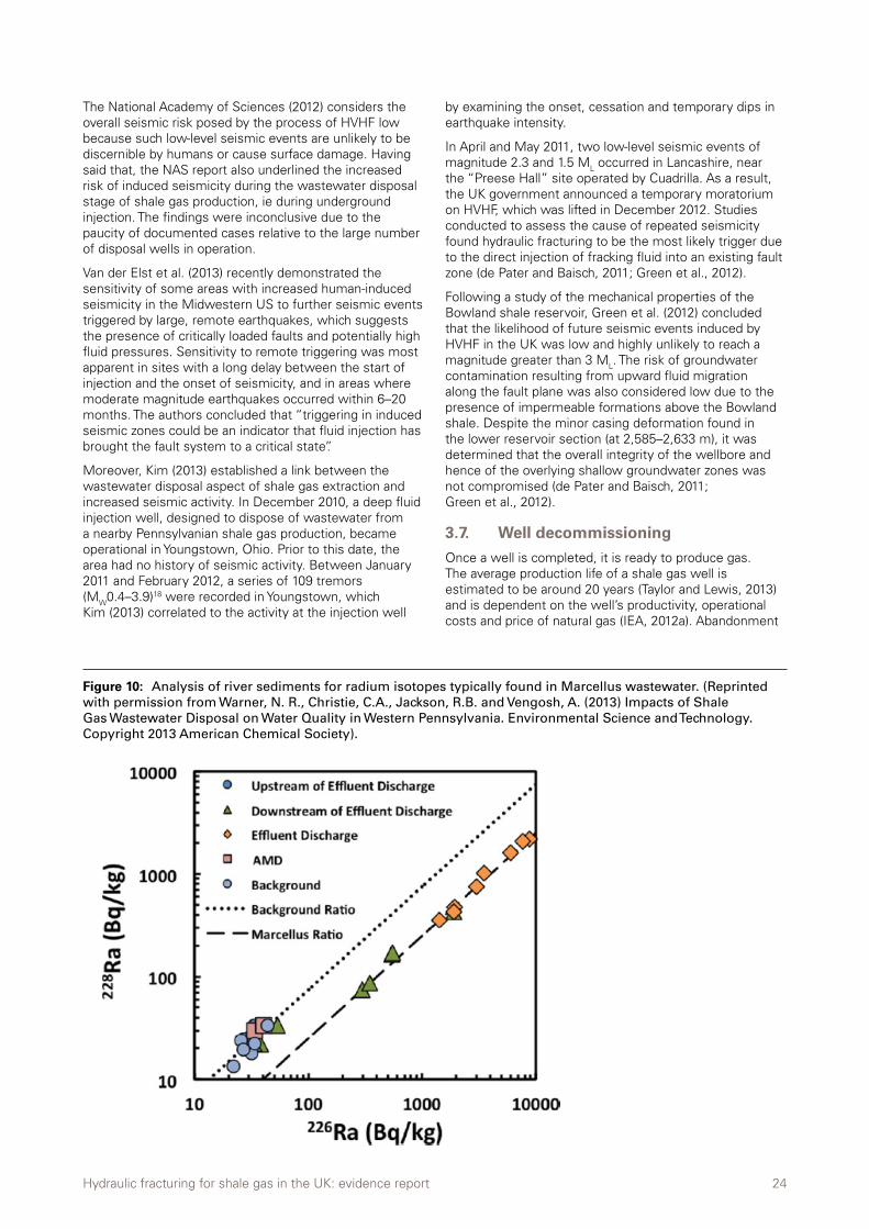
During and after well completion, the safe management of flowback and produced waters becomes of paramount importance to avoid risks of groundwater contamination resulting from accidents, runoff or surface spillages (Bloomfield, 2012). Another major concern is the contamination of surface waters by dissolved substances (eg radium-226)15, which can find their way into water bodies via the effluent discharge from a wastewater treatment works (WWTW) (Olmstead et al., 2013; Warner et al., 2013).
Figure 9: Status of water resource availability in England and Wales as per Cycle1-CAMS assessment (Source: EA, 2008)
Water available, 32%
No water available, 35%
Over-‐licensed, 18%
Over-‐abstracted,
15%
Hydraulic fracturing for shale gas in the UK: evidence report 22
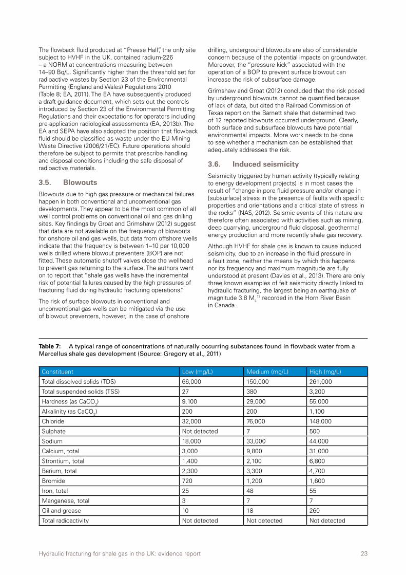
Minerals and organic compounds present in the shale formation dissolve into the injected fracking fluid, creating a hyper-saline formation brine that returns to the surface in the form of flowback water, which typically contains high levels of total dissolved solids (TDS), including several types of ions (eg chloride, sodium and calcium), heavy metals and organic compounds (Table 7). Notably, naturally occurring radioactive materials (NORM) are also found in the flowback water, at sufficiently high concentrations to characterise the wastewater as radioactive waste, necessitating a Radioactive Substances Permit by the operator and the wastewater treatment facilities that receive this type of waste. At present, however, no facility in the northwest of England is authorised by such a permit.
Due to the volumes of fluids involved and their chemical content, flowback water must be treated and disposed of carefully. Recent studies (Olmstead et al., 2013; Vengosh et al., 2013) show that the disposal of shale gas wastewaters to waterways in western Pennsylvania generated a highly saline environment (TDS up to 100,000 mg/L) and resulted in increased radioactivity in both downstream surface waters and river sediments.
Focusing on the Marcellus Shale in Pennsylvania, Olmstead et al. (2013) examined the impact of treated shale gas wastewater discharge by permitted treatment facilities on observed downstream concentrations of chloride and total suspended solids (TSS). Their results indicate that the treatment of HVHF waste by treatment plants in a catchment raises downstream chloride concentrations. They also reported that the presence of shale gas wells upstream in a catchment raised TSS concentrations downstream. Consideration of the impact of all components of flowback and produced water after
treatment on the receiving water body will be critical for the long-term sustainability of UK natural resources.
Warner et al. (2013) looked at the water quality and isotopic composition of discharged effluents, surface waters, and stream sediments associated with a treatment facility site in western Pennsylvania. The discharge of the effluent from the treatment facility increased downstream concentrations of chloride and bromide above baseline levels. Barium and radium were substantially (>90%) reduced in the treated effluents compared to concentrations in Marcellus Shale produced waters. Nonetheless, radium-226 levels in stream sediments (544–8,759 Bq/kg)16 at the point of discharge were 200 times greater than upstream and baseline sediment measurements (22–44 Bq/kg) and above radioactive waste disposal threshold regulations in the US, posing potential environmental risks of radium bioaccumulation in localised areas of shale gas wastewater disposal (Figure 10).
Historically, flowback water management options for some US shale plays have been limited by high concentrations of TDS in the flowback water, geography, geology and a lack of physical infrastructure. Until fairly recently, contaminated wastewater produced in US shale gas operations has been too costly to treat, so it has been re-injected deep underground into separate EPA-regulated wells designated for this purpose. Due to a rapid decrease of treatment costs of flowback water, however, a new industry has emerged in the last few years to treat and recycle this water for reuse in the fracturing of other wells. There are, however, limits to reuse with Gregory et al. (2011) reporting decreased effectiveness of friction reducers at high TDS concentrations.
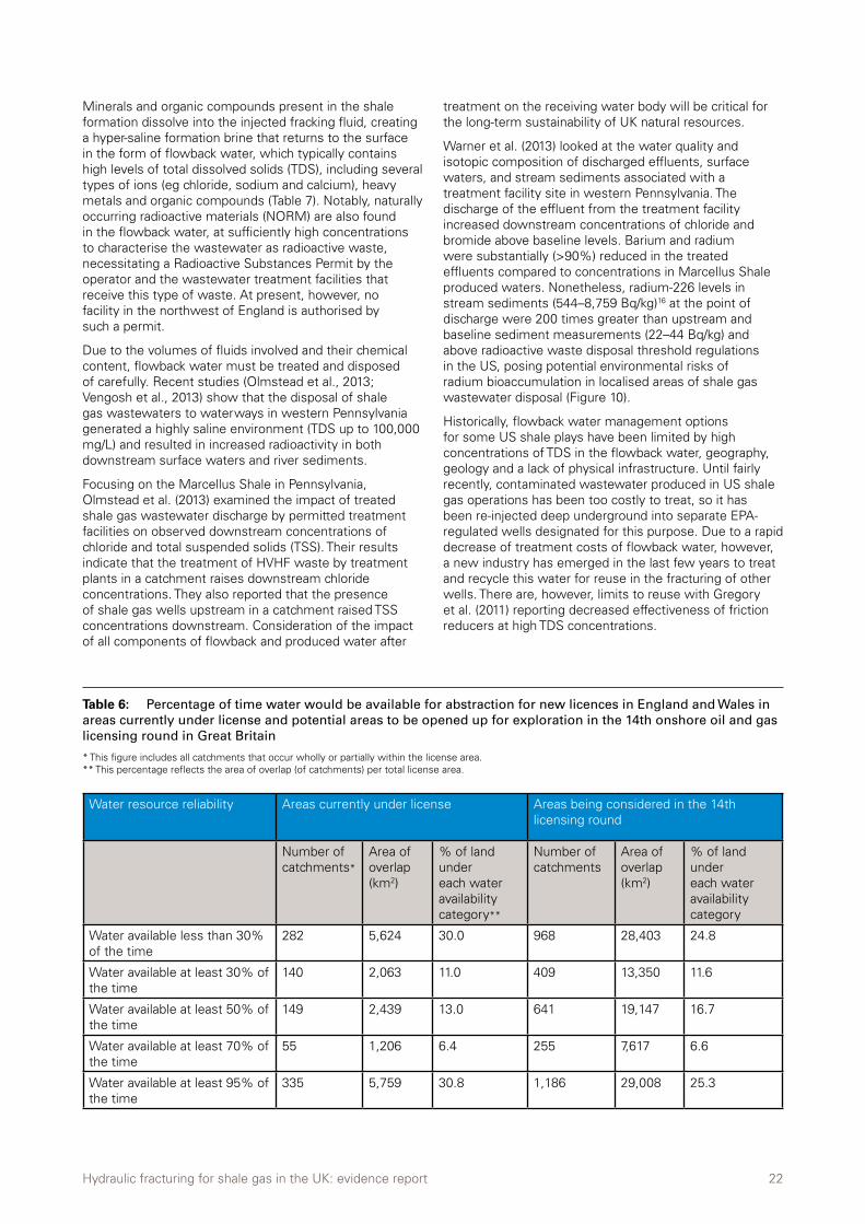
Water resource reliability Areas currently under license Areas being considered in the 14th licensing round
Number of catchments*
Area of overlap (km2)
% of land under each water availability category**
Number of catchments
Area of overlap (km2)
% of land under each water availability category
Water available less than 30% of the time
282 5,624 30.0 968 28,403 24.8
Water available at least 30% of the time
140 2,063 11.0 409 13,350 11.6
Water available at least 50% of the time
149 2,439 13.0 641 19,147 16.7
Water available at least 70% of the time
55 1,206 6.4 255 7,617 6.6
Water available at least 95% of the time
335 5,759 30.8 1,186 29,008 25.3
Table 6: Percentage of time water would be available for abstraction for new licences in England and Wales in areas currently under license and potential areas to be opened up for exploration in the 14th onshore oil and gas licensing round in Great Britain
* This figure includes all catchments that occur wholly or partially within the license area. ** This percentage reflects the area of overlap (of catchments) per total license area.
Hydraulic fracturing for shale gas in the UK: evidence report 23
The flowback fluid produced at “Preese Hall”, the only site subject to HVHF in the UK, contained radium-226 – a NORM at concentrations measuring between 14–90 Bq/L. Significantly higher than the threshold set for radioactive wastes by Section 23 of the Environmental Permitting (England and Wales) Regulations 2010 (Table 8; EA, 2011). The EA have subsequently produced a draft guidance document, which sets out the controls introduced by Section 23 of the Environmental Permitting Regulations and their expectations for operators including pre-application radiological assessments (EA, 2013b). The EA and SEPA have also adopted the position that flowback fluid should be classified as waste under the EU Mining Waste Directive (2006/21/EC). Future operations should therefore be subject to permits that prescribe handling and disposal conditions including the safe disposal of radioactive materials.
3.5. Blowouts
Blowouts due to high gas pressure or mechanical failures happen in both conventional and unconventional gas developments. They appear to be the most common of all well control problems on conventional oil and gas drilling sites. Key findings by Groat and Grimshaw (2012) suggest that data are not available on the frequency of blowouts for onshore oil and gas wells, but data from offshore wells indicate that the frequency is between 1–10 per 10,000 wells drilled where blowout preventers (BOP) are not fitted. These automatic shutoff valves close the wellhead to prevent gas returning to the surface. The authors went on to report that “shale gas wells have the incremental risk of potential failures caused by the high pressures of fracturing fluid during hydraulic fracturing operations.”
The risk of surface blowouts in conventional and unconventional gas wells can be mitigated via the use of blowout preventers, however, in the case of onshore
drilling, underground blowouts are also of considerable concern because of the potential impacts on groundwater. Moreover, the “pressure kick” associated with the operation of a BOP to prevent surface blowout can increase the risk of subsurface damage.
Grimshaw and Groat (2012) concluded that the risk posed by underground blowouts cannot be quantified because of lack of data, but cited the Railroad Commission of Texas report on the Barnett shale that determined two of 12 reported blowouts occurred underground. Clearly, both surface and subsurface blowouts have potential environmental impacts. More work needs to be done to see whether a mechanism can be established that adequately addresses the risk.
3.6. Induced seismicity
Seismicity triggered by human activity (typically relating to energy development projects) is in most cases the result of “change in pore fluid pressure and/or change in [subsurface] stress in the presence of faults with specific properties and orientations and a critical state of stress in the rocks” (NAS, 2012). Seismic events of this nature are therefore often associated with activities such as mining, deep quarrying, underground fluid disposal, geothermal energy production and more recently shale gas recovery.
Although HVHF for shale gas is known to cause induced seismicity, due to an increase in the fluid pressure in a fault zone, neither the means by which this happens nor its frequency and maximum magnitude are fully understood at present (Davies et al., 2013). There are only three known examples of felt seismicity directly linked to hydraulic fracturing, the largest being an earthquake of magnitude 3.8 ML
17 recorded in the Horn River Basin in Canada.
Constituent Low (mg/L) Medium (mg/L) High (mg/L)
Total dissolved solids (TDS) 66,000 150,000 261,000
Total suspended solids (TSS) 27 380 3,200
Hardness (as CaCO3) 9,100 29,000 55,000
Alkalinity (as CaCO3) 200 200 1,100
Chloride 32,000 76,000 148,000
Sulphate Not detected 7 500
Sodium 18,000 33,000 44,000
Calcium, total 3,000 9,800 31,000
Strontium, total 1,400 2,100 6,800
Barium, total 2,300 3,300 4,700
Bromide 720 1,200 1,600
Iron, total 25 48 55
Manganese, total 3 7 7
Oil and grease 10 18 260
Total radioactivity Not detected Not detected Not detected
Table 7: A typical range of concentrations of naturally occurring substances found in flowback water from a Marcellus shale gas development (Source: Gregory et al., 2011)
Hydraulic fracturing for shale gas in the UK: evidence report 24
The National Academy of Sciences (2012) considers the overall seismic risk posed by the process of HVHF low because such low-level seismic events are unlikely to be discernible by humans or cause surface damage. Having said that, the NAS report also underlined the increased risk of induced seismicity during the wastewater disposal stage of shale gas production, ie during underground injection. The findings were inconclusive due to the paucity of documented cases relative to the large number of disposal wells in operation.
Van der Elst et al. (2013) recently demonstrated the sensitivity of some areas with increased human-induced seismicity in the Midwestern US to further seismic events triggered by large, remote earthquakes, which suggests the presence of critically loaded faults and potentially high fluid pressures. Sensitivity to remote triggering was most apparent in sites with a long delay between the start of injection and the onset of seismicity, and in areas where moderate magnitude earthquakes occurred within 6–20 months. The authors concluded that “triggering in induced seismic zones could be an indicator that fluid injection has brought the fault system to a critical state”.
Moreover, Kim (2013) established a link between the wastewater disposal aspect of shale gas extraction and increased seismic activity. In December 2010, a deep fluid injection well, designed to dispose of wastewater from a nearby Pennsylvanian shale gas production, became operational in Youngstown, Ohio. Prior to this date, the area had no history of seismic activity. Between January 2011 and February 2012, a series of 109 tremors (MW0.4–3.9)18 were recorded in Youngstown, which Kim (2013) correlated to the activity at the injection well
by examining the onset, cessation and temporary dips in earthquake intensity.
In April and May 2011, two low-level seismic events of magnitude 2.3 and 1.5 ML occurred in Lancashire, near the “Preese Hall” site operated by Cuadrilla. As a result, the UK government announced a temporary moratorium on HVHF, which was lifted in December 2012. Studies conducted to assess the cause of repeated seismicity found hydraulic fracturing to be the most likely trigger due to the direct injection of fracking fluid into an existing fault zone (de Pater and Baisch, 2011; Green et al., 2012).
Following a study of the mechanical properties of the Bowland shale reservoir, Green et al. (2012) concluded that the likelihood of future seismic events induced by HVHF in the UK was low and highly unlikely to reach a magnitude greater than 3 ML. The risk of groundwater contamination resulting from upward fluid migration along the fault plane was also considered low due to the presence of impermeable formations above the Bowland shale. Despite the minor casing deformation found in the lower reservoir section (at 2,585–2,633 m), it was determined that the overall integrity of the wellbore and hence of the overlying shallow groundwater zones was not compromised (de Pater and Baisch, 2011; Green et al., 2012).
3.7. Well decommissioning
Once a well is completed, it is ready to produce gas. The average production life of a shale gas well is estimated to be around 20 years (Taylor and Lewis, 2013) and is dependent on the well’s productivity, operational costs and price of natural gas (IEA, 2012a). Abandonment
Figure 10: Analysis of river sediments for radium isotopes typically found in Marcellus wastewater. (Reprinted with permission from Warner, N. R., Christie, C.A., Jackson, R.B. and Vengosh, A. (2013) Impacts of Shale Gas Wastewater Disposal on Water Quality in Western Pennsylvania. Environmental Science and Technology. Copyright 2013 American Chemical Society).
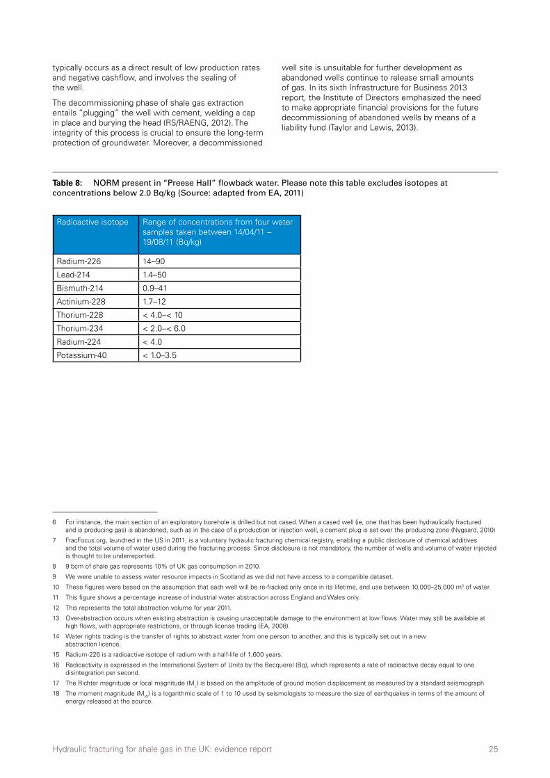
Hydraulic fracturing for shale gas in the UK: evidence report 25
typically occurs as a direct result of low production rates and negative cashflow, and involves the sealing of the well.
The decommissioning phase of shale gas extraction entails “plugging” the well with cement, welding a cap in place and burying the head (RS/RAENG, 2012). The integrity of this process is crucial to ensure the long-term protection of groundwater. Moreover, a decommissioned
well site is unsuitable for further development as abandoned wells continue to release small amounts of gas. In its sixth Infrastructure for Business 2013 report, the Institute of Directors emphasized the need to make appropriate financial provisions for the future decommissioning of abandoned wells by means of a liability fund (Taylor and Lewis, 2013).
Radioactive isotope Range of concentrations from four water samples taken between 14/04/11 – 19/08/11 (Bq/kg)
Radium-226 14–90
Lead-214 1.4–50
Bismuth-214 0.9–41
Actinium-228 1.7–12
Thorium-228 < 4.0–< 10
Thorium-234 < 2.0–< 6.0
Radium-224 < 4.0
Potassium-40 < 1.0–3.5
Table 8: NORM present in “Preese Hall” flowback water. Please note this table excludes isotopes at concentrations below 2.0 Bq/kg (Source: adapted from EA, 2011)
6 For instance, the main section of an exploratory borehole is drilled but not cased. When a cased well (ie, one that has been hydraulically fractured and is producing gas) is abandoned, such as in the case of a production or injection well, a cement plug is set over the producing zone (Nygaard, 2010)
7 FracFocus.org, launched in the US in 2011, is a voluntary hydraulic fracturing chemical registry, enabling a public disclosure of chemical additives and the total volume of water used during the fracturing process. Since disclosure is not mandatory, the number of wells and volume of water injected is thought to be underreported.
8 9 bcm of shale gas represents 10% of UK gas consumption in 2010.
9 We were unable to assess water resource impacts in Scotland as we did not have access to a compatible dataset.
10 These figures were based on the assumption that each well will be re-fracked only once in its lifetime, and use between 10,000–25,000 m3 of water.
11 This figure shows a percentage increase of industrial water abstraction across England and Wales only.
12 This represents the total abstraction volume for year 2011.
13 Over-abstraction occurs when existing abstraction is causing unacceptable damage to the environment at low flows. Water may still be available at high flows, with appropriate restrictions, or through license trading (EA, 2008).
14 Water rights trading is the transfer of rights to abstract water from one person to another, and this is typically set out in a new abstraction licence.
15 Radium-226 is a radioactive isotope of radium with a half-life of 1,600 years.
16 Radioactivity is expressed in the International System of Units by the Becquerel (Bq), which represents a rate of radioactive decay equal to one disintegration per second.
17 The Richter magnitude or local magnitude (ML) is based on the amplitude of ground motion displacement as measured by a standard seismograph
18 The moment magnitude (MW) is a logarithmic scale of 1 to 10 used by seismologists to measure the size of earthquakes in terms of the amount of energy released at the source.
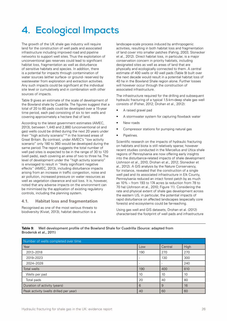
Hydraulic fracturing for shale gas in the UK: evidence report 26
4. Ecological Impacts The growth of the UK shale gas industry will require land for the construction of well pads and associated infrastructure including improved road and pipeline networks to support well sites. Thus the exploitation of unconventional gas reserves could lead to significant habitat loss, fragmentation as well as disturbance of sensitive habitats and species. In addition, there is a potential for impacts through contamination of water sources (either surface- or ground- reserves) by wastewater from exploration and extraction activities. Any such impacts could be significant at the individual site level or cumulatively and in combination with other sources of impacts.
Table 9 gives an estimate of the scale of development of the Bowland shale by Cuadrilla. The figures suggest that a total of 20 to 80 pads could be developed over a 15-year time period, each pad consisting of six to ten wells and covering approximately a hectare (ha) of land.
According to the latest government estimates (AMEC, 2013), between 1,440 and 2,880 (unconventional oil and gas) wells could be drilled during the next 20 years under their “high activity scenario”19 in the licensed areas of Great Britain. By contrast, under AMEC’s “low activity scenario” only 180 to 360 would be developed during the same period. The report suggests the total number of well pad sites is expected to be in the range of 30 to 120 (well pads), each covering an area of two to three ha. The level of development under the “high activity scenario” is envisaged to result in “likely significant negative effects” (AMEC, 2013), including disturbance impacts arising from an increase in traffic congestion, noise and air pollution, increased pressure on water resources as well as vegetation clearance and soil loss. It is, however, noted that any adverse impacts on the environment can be minimised by the application of existing regulatory controls, including the planning system.
4.1. Habitat loss and fragmentation
Recognised as one of the most serious threats to biodiversity (Kiviat, 2013), habitat destruction is a
landscape-scale process induced by anthropogenic activities, resulting in both habitat loss and fragmentation of land cover into smaller patches (Fahrig, 2003; Slonecker et al., 2012). Direct habitat loss, in particular, is a major conservation concern in priority habitats, including designated sites as well as areas of land that are physically and ecologically connected to them. A central estimate of 400 wells or 40 well pads (Table 9) built over the next decade would result in a potential habitat loss of 40 ha in the Bowland Shale region alone. Further losses will however occur through the construction of associated infrastructure.
The infrastructure required for the drilling and subsequent hydraulic fracturing of a typical 1.5-km-deep shale gas well consists of (Fisher, 2012; Drohan et al., 2012):
• A raised gravel pad
• A stormwater system for capturing flowback water
• New roads
• Compressor stations for pumping natural gas
• Pipelines.
Scientific research on the impacts of hydraulic fracturing on habitats and biota is still relatively sparse; however recent studies conducted in the Marcellus and Utica shale regions of Pennsylvania are now offering early insights into the disturbance-related impacts of shale development (Johnson et al., 2010; Drohan et al., 2012; Slonecker et al., 2012). A GIS analysis by the Nature Conservancy, for instance, revealed that the construction of a single well pad and its associated infrastructure in Elk County, Pennsylvania reduced an intact forest patch by as much as 10% – from 193 to 174 acres (a reduction from 78 to 70 ha) (Johnson et al., 2010; Figure 11). Considering the rate and physical extent of shale gas development across the eastern US, in particular, the potential impacts of rapid disturbance on affected landscapes (especially core forests) and ecosystems could be far-reaching.
Using gas well and GIS datasets, Drohan et al. (2012) characterised the footprint of well pads and infrastructure
Number of wells completed over time
Year Low Central High
2013–2018 190 270 270
2019–2023 - 130 300
2024–2028 - - 240
Total wells 190 400 810
Wells per pad 10 10 10
Total pads 20 40 80
Duration of activity (years) 6 9 16
Peak activity (wells drilled per year) 40 60 60
Table 9: Well development profile of the Bowland Shale for Cuadrilla (Source: adapted from Broderick et al., 2011)
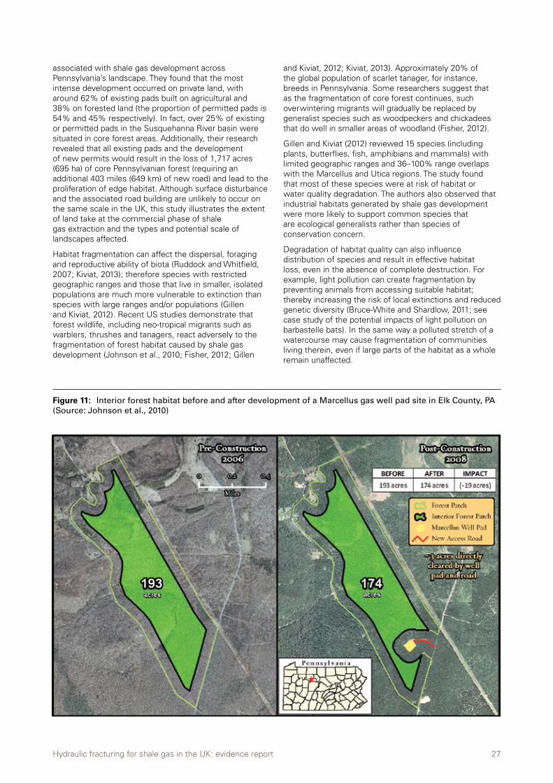
Hydraulic fracturing for shale gas in the UK: evidence report 27
associated with shale gas development across Pennsylvania’s landscape. They found that the most intense development occurred on private land, with around 62% of existing pads built on agricultural and 38% on forested land (the proportion of permitted pads is 54% and 45% respectively). In fact, over 25% of existing or permitted pads in the Susquehanna River basin were situated in core forest areas. Additionally, their research revealed that all existing pads and the development of new permits would result in the loss of 1,717 acres (695 ha) of core Pennsylvanian forest (requiring an additional 403 miles (649 km) of new road) and lead to the proliferation of edge habitat. Although surface disturbance and the associated road building are unlikely to occur on the same scale in the UK, this study illustrates the extent of land take at the commercial phase of shale gas extraction and the types and potential scale of landscapes affected.
Habitat fragmentation can affect the dispersal, foraging and reproductive ability of biota (Ruddock and Whitfield, 2007; Kiviat, 2013); therefore species with restricted geographic ranges and those that live in smaller, isolated populations are much more vulnerable to extinction than species with large ranges and/or populations (Gillen and Kiviat, 2012). Recent US studies demonstrate that forest wildlife, including neo-tropical migrants such as warblers, thrushes and tanagers, react adversely to the fragmentation of forest habitat caused by shale gas development (Johnson et al., 2010; Fisher, 2012; Gillen
and Kiviat, 2012; Kiviat, 2013). Approximately 20% of the global population of scarlet tanager, for instance, breeds in Pennsylvania. Some researchers suggest that as the fragmentation of core forest continues, such overwintering migrants will gradually be replaced by generalist species such as woodpeckers and chickadees that do well in smaller areas of woodland (Fisher, 2012).
Gillen and Kiviat (2012) reviewed 15 species (including plants, butterflies, fish, amphibians and mammals) with limited geographic ranges and 36–100% range overlaps with the Marcellus and Utica regions. The study found that most of these species were at risk of habitat or water quality degradation. The authors also observed that industrial habitats generated by shale gas development were more likely to support common species that are ecological generalists rather than species of conservation concern.
Degradation of habitat quality can also influence distribution of species and result in effective habitat loss, even in the absence of complete destruction. For example, light pollution can create fragmentation by preventing animals from accessing suitable habitat; thereby increasing the risk of local extinctions and reduced genetic diversity (Bruce-White and Shardlow, 2011; see case study of the potential impacts of light pollution on barbastelle bats). In the same way a polluted stretch of a watercourse may cause fragmentation of communities living therein, even if large parts of the habitat as a whole remain unaffected.
Figure 11: Interior forest habitat before and after development of a Marcellus gas well pad site in Elk County, PA (Source: Johnson et al., 2010)
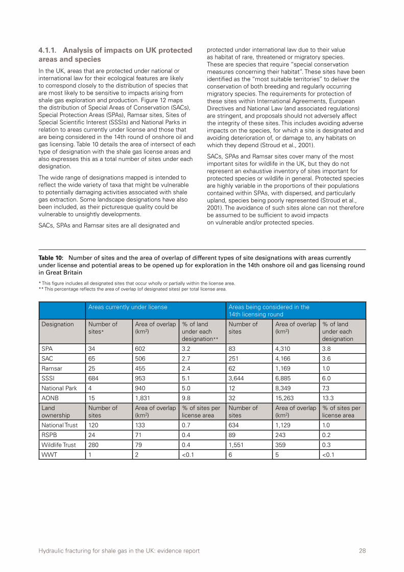
Hydraulic fracturing for shale gas in the UK: evidence report 28
4.1.1. Analysis of impacts on UK protected areas and species
In the UK, areas that are protected under national or international law for their ecological features are likely to correspond closely to the distribution of species that are most likely to be sensitive to impacts arising from shale gas exploration and production. Figure 12 maps the distribution of Special Areas of Conservation (SACs), Special Protection Areas (SPAs), Ramsar sites, Sites of Special Scientific Interest (SSSIs) and National Parks in relation to areas currently under license and those that are being considered in the 14th round of onshore oil and gas licensing. Table 10 details the area of intersect of each type of designation with the shale gas license areas and also expresses this as a total number of sites under each designation.
The wide range of designations mapped is intended to reflect the wide variety of taxa that might be vulnerable to potentially damaging activities associated with shale gas extraction. Some landscape designations have also been included, as their picturesque quality could be vulnerable to unsightly developments.
SACs, SPAs and Ramsar sites are all designated and
protected under international law due to their value as habitat of rare, threatened or migratory species. These are species that require ‘‘special conservation measures concerning their habitat’’. These sites have been identified as the ‘‘most suitable territories’’ to deliver the conservation of both breeding and regularly occurring migratory species. The requirements for protection of these sites within International Agreements, European Directives and National Law (and associated regulations) are stringent, and proposals should not adversely affect the integrity of these sites. This includes avoiding adverse impacts on the species, for which a site is designated and avoiding deterioration of, or damage to, any habitats on which they depend (Stroud et al., 2001).
SACs, SPAs and Ramsar sites cover many of the most important sites for wildlife in the UK, but they do not represent an exhaustive inventory of sites important for protected species or wildlife in general. Protected species are highly variable in the proportions of their populations contained within SPAs, with dispersed, and particularly upland, species being poorly represented (Stroud et al., 2001). The avoidance of such sites alone can not therefore be assumed to be sufficient to avoid impacts on vulnerable and/or protected species.
Areas currently under license Areas being considered in the 14th licensing round
Designation Number of sites*
Area of overlap (km2)
% of land under each designation**
Number of sites
Area of overlap (km2)
% of land under each designation
SPA 34 602 3.2 83 4,310 3.8
SAC 65 506 2.7 251 4,166 3.6
Ramsar 25 455 2.4 62 1,169 1.0
SSSI 684 953 5.1 3,644 6,885 6.0
National Park 4 940 5.0 12 8,349 7.3
AONB 15 1,831 9.8 32 15,263 13.3
Land ownership
Number of sites
Area of overlap (km2)
% of sites per license area
Number of sites
Area of overlap (km2)
% of sites per license area
National Trust 120 133 0.7 634 1,129 1.0
RSPB 24 71 0.4 89 243 0.2
Wildlife Trust 280 79 0.4 1,551 359 0.3
WWT 1 2 <0.1 6 5 <0.1
Table 10: Number of sites and the area of overlap of different types of site designations with areas currently under license and potential areas to be opened up for exploration in the 14th onshore oil and gas licensing round in Great Britain
* This figure includes all designated sites that occur wholly or partially within the license area. ** This percentage reflects the area of overlap (of designated sites) per total license area.
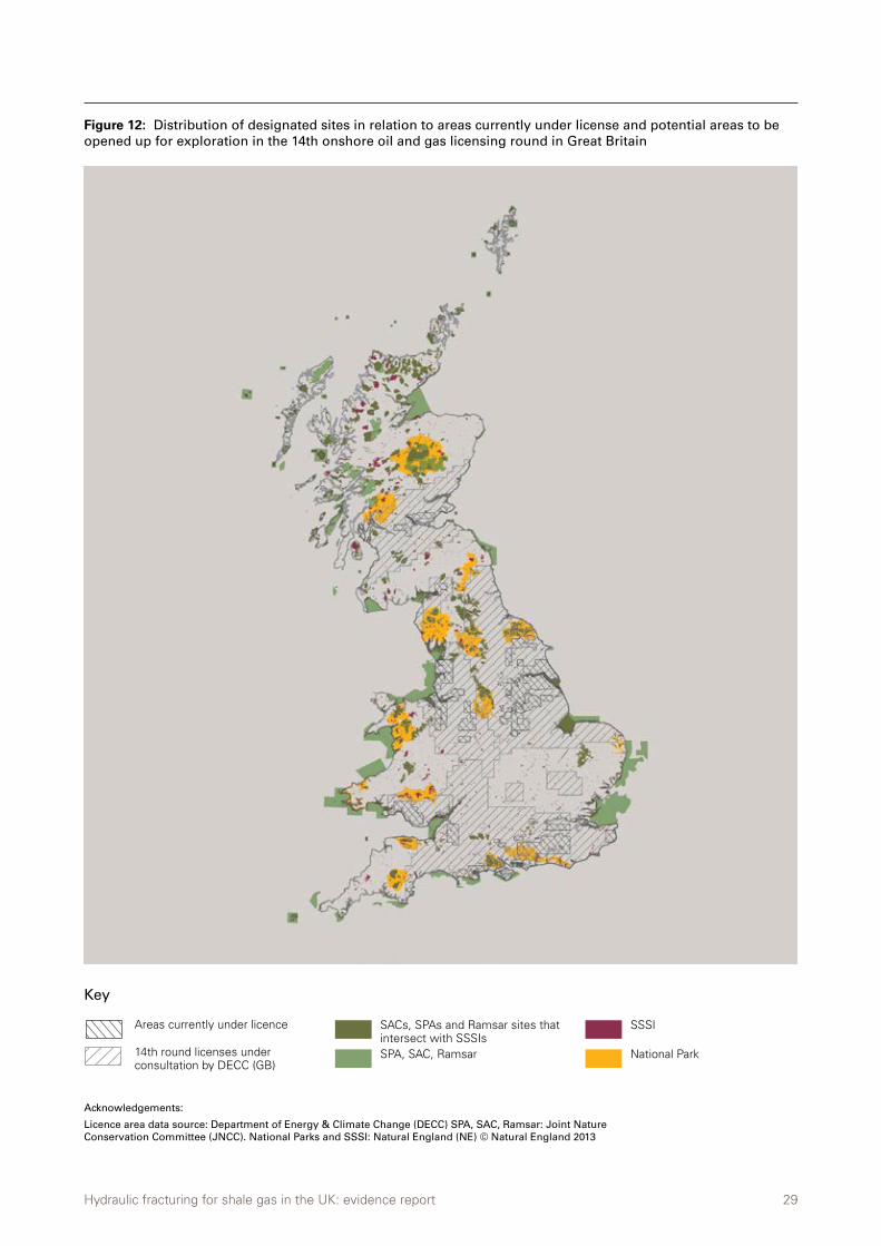
Hydraulic fracturing for shale gas in the UK: evidence report 29
Figure 12: Distribution of designated sites in relation to areas currently under license and potential areas to be opened up for exploration in the 14th onshore oil and gas licensing round in Great Britain
Key
Areas currently under licence
14th round licenses under consultation by DECC (GB)
Acknowledgements:
Licence area data source: Department of Energy & Climate Change (DECC) SPA, SAC, Ramsar: Joint Nature Conservation Committee (JNCC). National Parks and SSSI: Natural England (NE) © Natural England 2013
Key:
Acknowledgements:
0 6030 Km
E1:3,600,000Scale on A4 paperAreas currently under licence 14th roundlicences under consultation by DECC (GB)
Areas currently under licence and 14th round licences underconsultation by DECC (GB)
Licence area data source: Department of Energy & Climate Change (DECC)
Key:
Acknowledgements:
0 6030 Km
E1:3,600,000Scale on A4 paperAreas currently under licence 14th roundlicences under consultation by DECC (GB)
Areas currently under licence and 14th round licences underconsultation by DECC (GB)
Licence area data source: Department of Energy & Climate Change (DECC)
SACs, SPAs and Ramsar sites that intersect with SSSIsSPA, SAC, Ramsar
SSSI
National Park
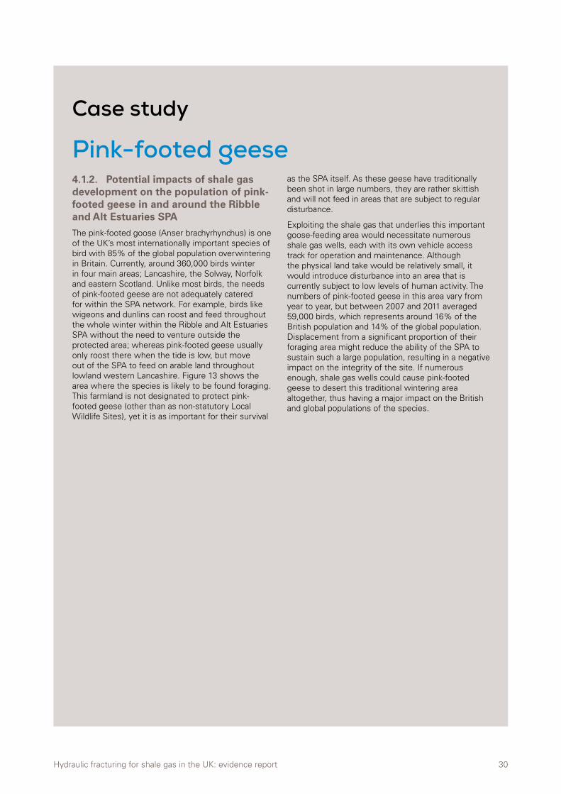
Hydraulic fracturing for shale gas in the UK: evidence report 30
4.1.2. Potential impacts of shale gas development on the population of pink-footed geese in and around the Ribble and Alt Estuaries SPA
The pink-footed goose (Anser brachyrhynchus) is one of the UK’s most internationally important species of bird with 85% of the global population overwintering in Britain. Currently, around 360,000 birds winter in four main areas; Lancashire, the Solway, Norfolk and eastern Scotland. Unlike most birds, the needs of pink-footed geese are not adequately catered for within the SPA network. For example, birds like wigeons and dunlins can roost and feed throughout the whole winter within the Ribble and Alt Estuaries SPA without the need to venture outside the protected area; whereas pink-footed geese usually only roost there when the tide is low, but move out of the SPA to feed on arable land throughout lowland western Lancashire. Figure 13 shows the area where the species is likely to be found foraging. This farmland is not designated to protect pink-footed geese (other than as non-statutory Local Wildlife Sites), yet it is as important for their survival
as the SPA itself. As these geese have traditionally been shot in large numbers, they are rather skittish and will not feed in areas that are subject to regular disturbance.
Exploiting the shale gas that underlies this important goose-feeding area would necessitate numerous shale gas wells, each with its own vehicle access track for operation and maintenance. Although the physical land take would be relatively small, it would introduce disturbance into an area that is currently subject to low levels of human activity. The numbers of pink-footed geese in this area vary from year to year, but between 2007 and 2011 averaged 59,000 birds, which represents around 16% of the British population and 14% of the global population. Displacement from a significant proportion of their foraging area might reduce the ability of the SPA to sustain such a large population, resulting in a negative impact on the integrity of the site. If numerous enough, shale gas wells could cause pink-footed geese to desert this traditional wintering area altogether, thus having a major impact on the British and global populations of the species.
Case study
Pink-footed geese
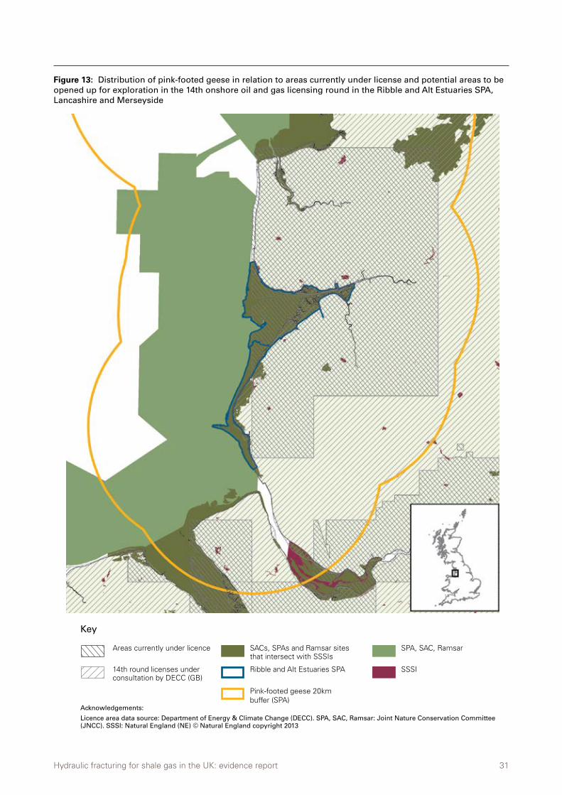
Hydraulic fracturing for shale gas in the UK: evidence report 31
Figure 13: Distribution of pink-footed geese in relation to areas currently under license and potential areas to be opened up for exploration in the 14th onshore oil and gas licensing round in the Ribble and Alt Estuaries SPA, Lancashire and Merseyside
Key
Areas currently under licence
14th round licenses under consultation by DECC (GB)
Acknowledgements:
Licence area data source: Department of Energy & Climate Change (DECC). SPA, SAC, Ramsar: Joint Nature Conservation Committee (JNCC). SSSI: Natural England (NE) © Natural England copyright 2013
Key:
Acknowledgements:
0 6030 Km
E1:3,600,000Scale on A4 paperAreas currently under licence 14th roundlicences under consultation by DECC (GB)
Areas currently under licence and 14th round licences underconsultation by DECC (GB)
Licence area data source: Department of Energy & Climate Change (DECC)
Key:
Acknowledgements:
0 6030 Km
E1:3,600,000Scale on A4 paperAreas currently under licence 14th roundlicences under consultation by DECC (GB)
Areas currently under licence and 14th round licences underconsultation by DECC (GB)
Licence area data source: Department of Energy & Climate Change (DECC)
SACs, SPAs and Ramsar sites that intersect with SSSIs
Ribble and Alt Estuaries SPA
Pink-footed geese 20km buffer (SPA)
SPA, SAC, Ramsar
SSSI
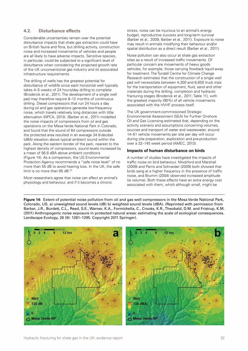
Hydraulic fracturing for shale gas in the UK: evidence report 32
4.2. Disturbance effects
Considerable uncertainties remain over the potential disturbance impacts that shale gas extraction could have on British fauna and flora, but drilling activity, construction noise and increased movements of vehicles and people are all likely to have adverse impacts. Sensitive species, in particular, could be subjected to a significant level of disturbance when considering the projected growth rate of the UK unconventional gas industry and its associated infrastructure requirements.
The drilling of wells has the greatest potential for disturbance of wildlife since each horizontal well typically takes 4–5 weeks of 24 hours/day drilling to complete (Broderick et al., 2011). The development of a single well pad may therefore require 8–12 months of continuous drilling. Diesel compressors that run 24 hours a day during oil and gas operations generate low-frequency noise, which travels relatively long distances with little attenuation (NPCA, 2013). (Barber et al., 2011) modelled the noise impacts of compressors from oil and gas operations on the Mesa Verde National Park in Colorado, and found that the sound of 64 compressors outside the protected area resulted in an average 34.8-decibel (dBA) elevation above typical ambient sound within the park. Along the eastern border of the park, nearest to the highest density of compressors, sound levels increased by a mean of 56.8 dBA above ambient conditions (Figure 14). As a comparison, the US Environmental Protection Agency recommends a “safe noise level” of no more than 55 dB to avoid hearing loss. In the UK, the safe limit is no more than 85 dB.20
Most researchers agree that noise can affect an animal’s physiology and behaviour, and if it becomes a chronic
stress, noise can be injurious to an animal’s energy budget, reproductive success and long-term survival (Barber et al., 2009; Barber et al., 2011). Exposure to noise may result in animals modifying their behaviour and/or spatial distribution as a direct result (Barber et al., 2011).
Noise pollution can also occur at shale gas extraction sites as a result of increased traffic movements. Of particular concern are movements of heavy goods vehicles, for example, those carrying flowback liquid away for treatment. The Tyndall Centre for Climate Change Research estimates that the construction of a single well pad will necessitate between 4,300 and 6,600 truck trips for the transportation of equipment, fluid, sand and other materials during the drilling, completion and hydraulic fracturing stages (Broderick et al., 2011; Table 11), with the greatest majority (90%) of all vehicle movements associated with the HVHF process itself.
The UK government-commissioned Strategic Environmental Assessment (SEA) for Further Onshore Oil and Gas Licensing estimated that, depending on the activity scenario and assumptions concerning volumes, sources and transport of water and wastewater, around 14–51 vehicle movements per site per day will occur during site preparation, exploration and pre-production over a 32–145 week period (AMEC, 2013).
Impacts of human disturbance on birds
A number of studies have investigated the impacts of traffic noise on bird behaviour. Mockford and Marshall (2009) and Parris and Schneider (2009) both showed that birds sang at a higher frequency in the presence of traffic noise, and Brumm (2004) observed increased amplitude (ie volume). Both these effects have an extra energy cost associated with them, which although small, might be
Figure 14: Extent of potential noise pollution from oil and gas well compressors in the Mesa Verde National Park, Colorado, US. a) unweighted sound levels (dB) b) weighted sound levels (dBA). (Reprinted with permission from Barber, J.R., Burdett, C.L., Reed, S.E., Warner, K.A., Formichella, C., Crooks, K.R., Theobald, D.M. and Fristrup, K.M. (2011) Anthropogenic noise exposure in protected natural areas: estimating the scale of ecological consequences. Landscape Ecology, 26 (9): 1281–1295. Copyright 2011 Springer).
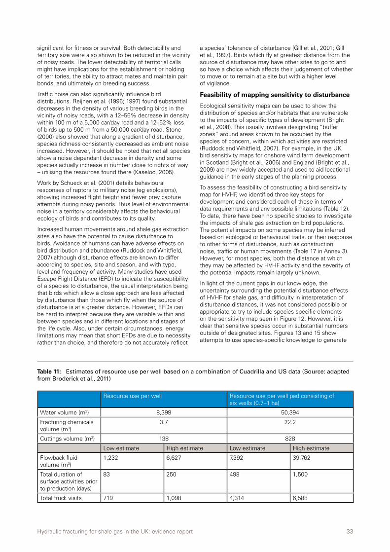
Hydraulic fracturing for shale gas in the UK: evidence report 33
significant for fitness or survival. Both detectability and territory size were also shown to be reduced in the vicinity of noisy roads. The lower detectability of territorial calls might have implications for the establishment or holding of territories, the ability to attract mates and maintain pair bonds, and ultimately on breeding success.
Traffic noise can also significantly influence bird distributions. Reijnen et al. (1996; 1997) found substantial decreases in the density of various breeding birds in the vicinity of noisy roads, with a 12–56% decrease in density within 100 m of a 5,000 car/day road and a 12–52% loss of birds up to 500 m from a 50,000 car/day road. Stone (2000) also showed that along a gradient of disturbance, species richness consistently decreased as ambient noise increased. However, it should be noted that not all species show a noise dependant decrease in density and some species actually increase in number close to rights of way – utilising the resources found there (Kaseloo, 2005).
Work by Schueck et al. (2001) details behavioural responses of raptors to military noise (eg explosions), showing increased flight height and fewer prey capture attempts during noisy periods. Thus level of environmental noise in a territory considerably affects the behavioural ecology of birds and contributes to its quality.
Increased human movements around shale gas extraction sites also have the potential to cause disturbance to birds. Avoidance of humans can have adverse effects on bird distribution and abundance (Ruddock and Whitfield, 2007) although disturbance effects are known to differ according to species, site and season, and with type, level and frequency of activity. Many studies have used Escape Flight Distance (EFD) to indicate the susceptibility of a species to disturbance, the usual interpretation being that birds which allow a close approach are less affected by disturbance than those which fly when the source of disturbance is at a greater distance. However, EFDs can be hard to interpret because they are variable within and between species and in different locations and stages of the life cycle. Also, under certain circumstances, energy limitations may mean that short EFDs are due to necessity rather than choice, and therefore do not accurately reflect
a species’ tolerance of disturbance (Gill et al., 2001; Gill et al., 1997). Birds which fly at greatest distance from the source of disturbance may have other sites to go to and so have a choice which affects their judgement of whether to move or to remain at a site but with a higher level of vigilance.
Feasibility of mapping sensitivity to disturbance
Ecological sensitivity maps can be used to show the distribution of species and/or habitats that are vulnerable to the impacts of specific types of development (Bright et al., 2008). This usually involves designating “buffer zones” around areas known to be occupied by the species of concern, within which activities are restricted (Ruddock and Whitfield, 2007). For example, in the UK, bird sensitivity maps for onshore wind farm development in Scotland (Bright et al., 2006) and England (Bright et al., 2009) are now widely accepted and used to aid locational guidance in the early stages of the planning process.
To assess the feasibility of constructing a bird sensitivity map for HVHF, we identified three key steps for development and considered each of these in terms of data requirements and any possible limitations (Table 12). To date, there have been no specific studies to investigate the impacts of shale gas extraction on bird populations. The potential impacts on some species may be inferred based on ecological or behavioural traits, or their response to other forms of disturbance, such as construction noise, traffic or human movements (Table 17 in Annex 3). However, for most species, both the distance at which they may be affected by HVHF activity and the severity of the potential impacts remain largely unknown.
In light of the current gaps in our knowledge, the uncertainty surrounding the potential disturbance effects of HVHF for shale gas, and difficulty in interpretation of disturbance distances, it was not considered possible or appropriate to try to include species specific elements on the sensitivity map seen in Figure 12. However, it is clear that sensitive species occur in substantial numbers outside of designated sites. Figures 13 and 15 show attempts to use species-specific knowledge to generate
Resource use per well Resource use per well pad consisting of six wells (0.7–1 ha)
Water volume (m3) 8,399 50,394
Fracturing chemicals volume (m3)
3.7 22.2
Cuttings volume (m3) 138 828
Low estimate High estimate Low estimate High estimate
Flowback fluid volume (m3)
1,232 6,627 7,392 39,762
Total duration of surface activities prior to production (days)
83 250 498 1,500
Total truck visits 719 1,098 4,314 6,588
Table 11: Estimates of resource use per well based on a combination of Cuadrilla and US data (Source: adapted from Broderick et al., 2011)
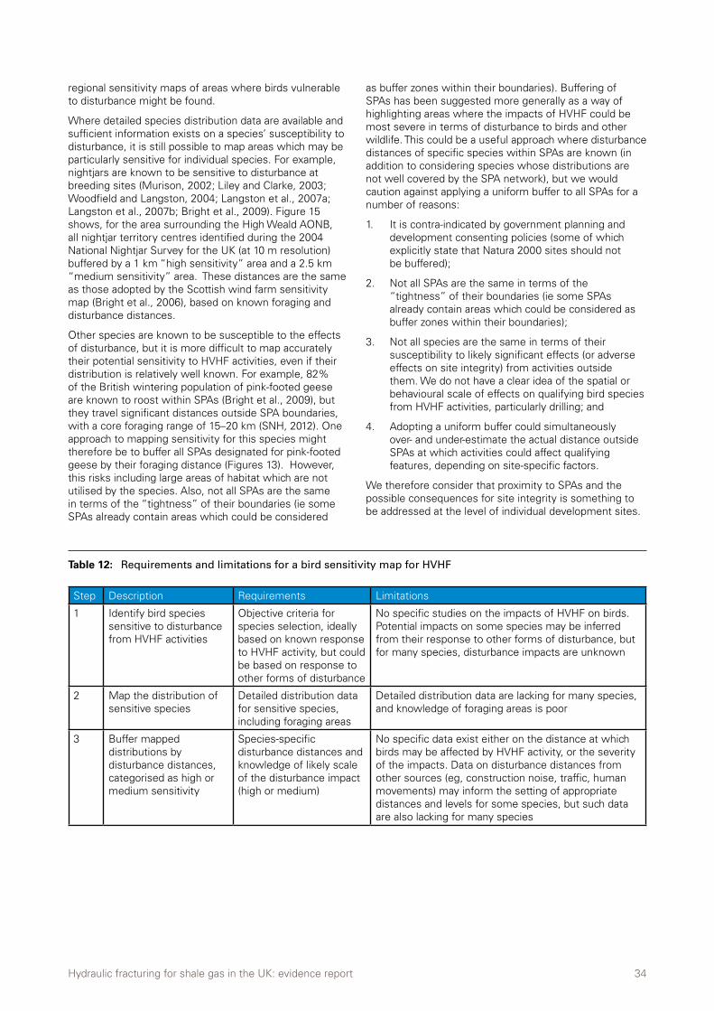
Hydraulic fracturing for shale gas in the UK: evidence report 34
regional sensitivity maps of areas where birds vulnerable to disturbance might be found.
Where detailed species distribution data are available and sufficient information exists on a species’ susceptibility to disturbance, it is still possible to map areas which may be particularly sensitive for individual species. For example, nightjars are known to be sensitive to disturbance at breeding sites (Murison, 2002; Liley and Clarke, 2003; Woodfield and Langston, 2004; Langston et al., 2007a; Langston et al., 2007b; Bright et al., 2009). Figure 15 shows, for the area surrounding the High Weald AONB, all nightjar territory centres identified during the 2004 National Nightjar Survey for the UK (at 10 m resolution) buffered by a 1 km “high sensitivity” area and a 2.5 km “medium sensitivity” area. These distances are the same as those adopted by the Scottish wind farm sensitivity map (Bright et al., 2006), based on known foraging and disturbance distances.
Other species are known to be susceptible to the effects of disturbance, but it is more difficult to map accurately their potential sensitivity to HVHF activities, even if their distribution is relatively well known. For example, 82% of the British wintering population of pink-footed geese are known to roost within SPAs (Bright et al., 2009), but they travel significant distances outside SPA boundaries, with a core foraging range of 15–20 km (SNH, 2012). One approach to mapping sensitivity for this species might therefore be to buffer all SPAs designated for pink-footed geese by their foraging distance (Figures 13). However, this risks including large areas of habitat which are not utilised by the species. Also, not all SPAs are the same in terms of the “tightness” of their boundaries (ie some SPAs already contain areas which could be considered
as buffer zones within their boundaries). Buffering of SPAs has been suggested more generally as a way of highlighting areas where the impacts of HVHF could be most severe in terms of disturbance to birds and other wildlife. This could be a useful approach where disturbance distances of specific species within SPAs are known (in addition to considering species whose distributions are not well covered by the SPA network), but we would caution against applying a uniform buffer to all SPAs for a number of reasons:
1. It is contra-indicated by government planning and development consenting policies (some of which explicitly state that Natura 2000 sites should not be buffered);
2. Not all SPAs are the same in terms of the “tightness” of their boundaries (ie some SPAs already contain areas which could be considered as buffer zones within their boundaries);
3. Not all species are the same in terms of their susceptibility to likely significant effects (or adverse effects on site integrity) from activities outside them. We do not have a clear idea of the spatial or behavioural scale of effects on qualifying bird species from HVHF activities, particularly drilling; and
4. Adopting a uniform buffer could simultaneously over- and under-estimate the actual distance outside SPAs at which activities could affect qualifying features, depending on site-specific factors.
We therefore consider that proximity to SPAs and the possible consequences for site integrity is something to be addressed at the level of individual development sites.
Step Description Requirements Limitations
1 Identify bird species sensitive to disturbance from HVHF activities
Objective criteria for species selection, ideally based on known response to HVHF activity, but could be based on response to other forms of disturbance
No specific studies on the impacts of HVHF on birds. Potential impacts on some species may be inferred from their response to other forms of disturbance, but for many species, disturbance impacts are unknown
2 Map the distribution of sensitive species
Detailed distribution data for sensitive species, including foraging areas
Detailed distribution data are lacking for many species, and knowledge of foraging areas is poor
3 Buffer mapped distributions by disturbance distances, categorised as high or medium sensitivity
Species-specific disturbance distances and knowledge of likely scale of the disturbance impact (high or medium)
No specific data exist either on the distance at which birds may be affected by HVHF activity, or the severity of the impacts. Data on disturbance distances from other sources (eg, construction noise, traffic, human movements) may inform the setting of appropriate distances and levels for some species, but such data are also lacking for many species
Table 12: Requirements and limitations for a bird sensitivity map for HVHF
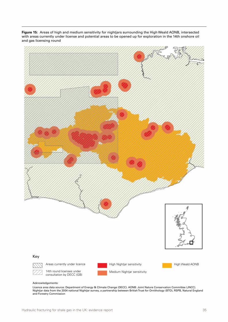
Hydraulic fracturing for shale gas in the UK: evidence report 35
Figure 15: Areas of high and medium sensitivity for nightjars surrounding the High Weald AONB, intersected with areas currently under license and potential areas to be opened up for exploration in the 14th onshore oil and gas licensing round
Key
Areas currently under licence
14th round licenses under consultation by DECC (GB)
Acknowledgements:
Licence area data source: Department of Energy & Climate Change (DECC). AONB: Joint Nature Conservation Committee (JNCC). Nightjar data from the 2004 national Nightjar survey, a partnership between British Trust for Ornithology (BTO), RSPB, Natural England and Forestry Commission
Key:
Acknowledgements:
0 6030 Km
E1:3,600,000Scale on A4 paperAreas currently under licence 14th roundlicences under consultation by DECC (GB)
Areas currently under licence and 14th round licences underconsultation by DECC (GB)
Licence area data source: Department of Energy & Climate Change (DECC)
Key:
Acknowledgements:
0 6030 Km
E1:3,600,000Scale on A4 paperAreas currently under licence 14th roundlicences under consultation by DECC (GB)
Areas currently under licence and 14th round licences underconsultation by DECC (GB)
Licence area data source: Department of Energy & Climate Change (DECC)
High Nightjar sensitivity
Medium Nightjar sensitivity
High Weald AONB

Hydraulic fracturing for shale gas in the UK: evidence report 36
4.2.1. Potential impacts of light pollution on barbastelle bats
Recently submitted plans for exploratory drilling for shale gas in the Weald Basin included proposals for a 45-metre derrick to be lit 24 hours a day, with additional lighting required for safety reasons. The following case study examines the adverse impacts of this type of activity on the protected barbastelle bats.
By examining satellite measurements of artificial light at night, a joint study by the Campaign to Protect Rural England and the British Astronomical Association (CPRE, 2003) established that light pollution is a rapidly growing problem across the UK, with severe to high light pollution affecting almost a quarter of England (Figure 16). Moreover, the impacts of artificial light on wildlife and the environment were recently highlighted by the Royal Commission on Environmental Pollution (RCEP, 2009), which stated that “there is potential for some aspect of life and its rhythms – migration, reproduction, feeding – to be affected [by artificial light. A] well known example is the effect on the feeding of bats caused by insects clustering around outdoor light sources”.
Bats are widely recognised as indicators of biodiversity and the barbastelle Barbastella barbastellus is a good example. It is an Annex 2 listed species on the EC Habitats Directive with a limited number of confirmed roosting populations in woodlands in southern Britain, including The Mens and Ebernoe Common, both of which are designated as SACs. With its diverse habitat requirements ranging from dense old growth woodlands along woody corridors to wet grassland feeding areas, the barbastelle is dependent on sensitive management at a landscape scale (Howorth, 2008).
The population of barbastelle bats in Ebernoe Common is probably the best studied in the UK. The bats breeding in Ebernoe Common SAC were first radio-tracked in 1998 to identify nursery roosts and flightlines. In summer 2008, the radio-tracking exercise was repeated to identify and map flightlines and forage areas and this was also extended to The Mens SAC. Greenaway (2008; Figure 17) found that:
1 Flightlines were often over 5 km long and in most cases followed watercourses and woodland cover;
2 Individual bats regularly used the same flightline for extended periods.
The study concluded that major threats to the species were those affecting any of their roosts, forage areas and flightline habitats and that, although the roosting SAC woodland itself was not threatened, the isolation of a colony from its forage areas by loss of cover along connecting flightlines posed a high risk to the barbastelle population (Greenaway, 2008). Hence, if their flightline is rendered unusable by artificial lighting, bats could be cut off from their foraging habitats, making it harder for them to hunt and survive. Greenaway (2008) cites an example of this where a large floodlit pumping station to the southwest of Pulborough, West Sussex caused an apparent interruption to the pattern of forage areas by the Ebernoe Common’s barbastelle bats, despite the presence of commoner (less light sensitive) species (F. Greenaway, pers. comm.). In addition, there is preliminary evidence that barbastelle bats could be responsive to light pollution (Murphy et al., 2009).
Stone et al. (2009) provide further evidence of the avoidance of light by bats. They installed high-pressure sodium lights that mimic the intensity and light spectra of streetlights along the commuting routes of lesser horseshoe bats Rhinolophus hipposideros. The authors found that bat activity was reduced dramatically and that the onset of commuting behaviour was delayed in the presence of lighting, with no evidence of habituation. These results demonstrate that light pollution can have significant negative impacts upon bat commuting and foraging behaviour.
Further work (Stone et al., 2012) demonstrates that the response to lighting is species specific. Slower flying species show a response to LED lighting whilst fast flying species do not show the same response. Moreover, research (Boldogh et al., 2007) found that artificial lighting close to roost sites can affect the emergence times of bats and that this has a corresponding effect on the physiology (body mass and size) of juvenile bats, possibly resulting in serious consequences for the colony.
Case study
Barbastelle bats
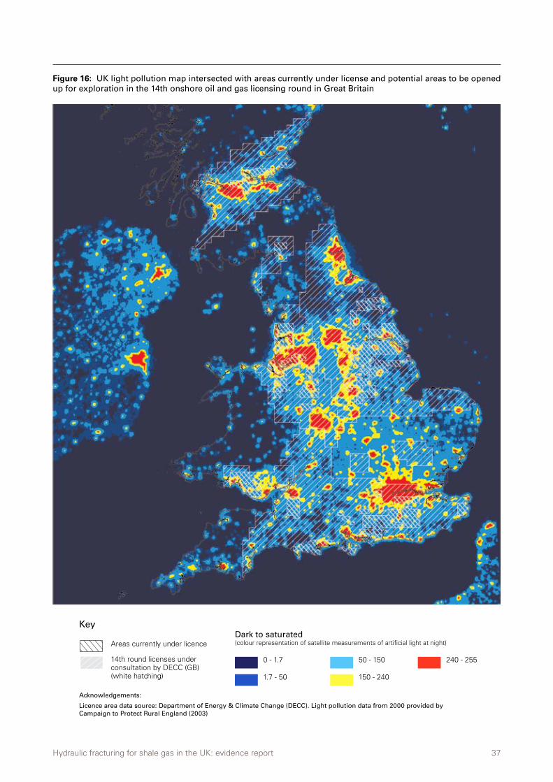
Hydraulic fracturing for shale gas in the UK: evidence report 37
Figure 16: UK light pollution map intersected with areas currently under license and potential areas to be opened up for exploration in the 14th onshore oil and gas licensing round in Great Britain
Key
Areas currently under licence
14th round licenses under consultation by DECC (GB) (white hatching)
Acknowledgements:
Licence area data source: Department of Energy & Climate Change (DECC). Light pollution data from 2000 provided by Campaign to Protect Rural England (2003)
Key:
Acknowledgements:
0 6030 Km
E1:3,600,000Scale on A4 paperAreas currently under licence 14th roundlicences under consultation by DECC (GB)
Areas currently under licence and 14th round licences underconsultation by DECC (GB)
Licence area data source: Department of Energy & Climate Change (DECC)
Dark to saturated (colour representation of satellite measurements of artificial light at night)
0 - 1.7
1.7 - 50
50 - 150
150 - 240
240 - 255
Hydraulic fracturing for shale gas in the UK: evidence report 38
Figure 17: Map showing flightlines of barbastelle bat populations at The Mens and Ebernoe Common SAC, intersected with areas currently under license and potential areas to be opened up for exploration in the 14th onshore oil and gas licensing round
Key
Areas currently under licence
14th round licenses under consultation by DECC (GB)(white hatching)
Acknowledgements:
Licence area data source: Department of Energy & Climate Change (DECC). SAC: Joint Nature Conservation Committee (JNCC). Light pollution data from 2000 provided by Campaign to Protect Rural England (2003). Barbastelle data: © Sussex Wildlife Trust
Key:
Acknowledgements:
0 6030 Km
E1:3,600,000Scale on A4 paperAreas currently under licence 14th roundlicences under consultation by DECC (GB)
Areas currently under licence and 14th round licences underconsultation by DECC (GB)
Licence area data source: Department of Energy & Climate Change (DECC)
Dark to saturated
150 - 240
1.7 - 50
0 - 1.7
50 - 150
240 - 255kernels (areas of activity for each bat or foraging areas)
Bat flight lines
SAC (The Mens and Ebernoe common)
Hydraulic fracturing for shale gas in the UK: evidence report 39
4.3. Impacts on aquatic biodiversity
In addition to surface disturbance, potential threats to priority habitats and species can occur via the contamination of surface water or shallow groundwater from hydraulic fracturing activities. Bamberger and Oswald (2012), for instance, assessed the potential impacts to livestock from well water contamination. The authors recorded cases of impaired reproductive ability (eg difficulty breeding or abnormalities in offspring) as well as fatality in cattle exposed to fracturing fluids either from spills or leaky wastewater pools. Studies such as this one demonstrate that the water contamination impacts of gas drilling are a significant consideration for animal health.
As outlined in Section 3.4, large volumes of waste fluids with high concentrations of total dissolved solids (TDS) containing several types of ions (eg calcium, magnesium and chloride), heavy metals as well as organic compounds (eg hydrocarbons, dissolved light gases, chemical additives from the HVHF fluid) are produced during shale gas operations. Average TDS concentrations in post-HVHF wastewaters range from 800 to 300,000 mg/L, whereas typical ocean water concentration is 35,000 mg/L and freshwater concentration is 100–500 mg/L (Gregory et al., 2011; Olmstead et al., 2013). In the UK, for example, most rivers and lakes have chloride concentrations of less than 50 mg/L, however the spatial distribution of streamwater chloride concentrations between upland and lowland areas can vary significantly throughout the catchment depending on land use characteristics (Smart et al., 2001).
Standard wastewater treatment works (WWTW) are not designed to handle hydraulic fracturing wastewater21, ie heavy metals and salts. The main technology that would allow this is ultrafiltration and reverse osmosis – something more typically found in state of the art drinking water treatment works dealing with difficult to treat pollutants. Such an approach to waste treatment is costly and energy intensive.
In the UK, the regulatory regime places controls on direct discharge of post-HVHF wastewater, and prohibits injection into abandoned wells or storage of flowback or produced waters in open surface lagoons (ie disposal methods that that are among the most widely adopted in the US). The EA (2013b), for instance, “expect(s) reuse of flowback fluid to be an element of any [Waste Management] Plan, but recognise(s) that offsite disposal may be proposed at the exploration stage”. Moreover, flowback or produced waters containing sufficiently high concentrations of naturally occurring radioactive materials (NORM) are classed as radioactive waste, and hence the operator and the WWTW require a Radioactive Substances Permit for its safe disposal. At present, there are no wastewater treatment facilities in the northwest of England authorised by such a permit.
Research into the environmental impacts of HVHF fluids and liquid wastes on the biota of the primary shale gas producing regions in the US is limited, however a number of recent studies have identified potential adverse impacts. Gillen and Kiviat (2012) reviewed the ranges and ecological requirements of 15 species of animals and plants with restricted geographic ranges and a high degree of overlap within the Marcellus and Utica shale regions to determine their vulnerability to shale gas activities. Of the studied species, over 70% (11) were known to be sensitive to the degradation of water quality (namely eight species of salamander, two of fish and a vascular plant), making them particularly vulnerable to HVHF impacts, such as elevated salinity or sediment pollution.
Papoulias and Velasco (2013) studied the potential effect of post-HVHF water quality on the threatened blackside dace Chrosomus cumberlandensis in Acorn Fork, a small Appalachian creek designated by Kentucky as an Outstanding State Resource Water. Following the spill of hydraulic fracturing fluid into the stream, low pH and toxic concentrations of heavy metals were observed in the affected waters, resulting in a significant die-off of aquatic life. Samples taken a month after the pollution incident demonstrated that fish exposed to contamination showed signs of distress and had a higher incidence of gill lesions than unexposed reference fish.
Moreover, Entrekin et al. (2011) positively correlated stream turbidity with the density of gas wells in the Fayetteville shale play, which stretches across the US state of Arkansas. Sediment pollution of streams and rivers arising as a result of poor erosion control at shale gas sites or the transportation of heavy equipment on rural roads mobilising mineral particles in runoff or airborne dust could potentially harm benthic invertebrates and fish (Kiviat, 2013); native brook trout and freshwater mussels are especially vulnerable to increased sediment loads.
Impacts of HVHF wastewater on vegetation were documented in a 2011 study that mimicked the effects of an accidental spill of nearly 80,000 gallons (303 m3) of wastewater on a half-acre (0.2-ha) plot of the US Forest Service’s Fernow Experimental Forest (Adams, 2011). The wastewater contained chloride levels that were within state standards for disposal on the landscape; however the large quantities applied to a small area resulted in an estimated 4,500 kg of chloride per acre (concentrations of sodium and chloride in the application area were 50 times higher than in the nearby untreated plots). Two years after the fluids were applied, 56% of trees had died, likely as a result of high TDS concentrations.
Hydraulic fracturing for shale gas in the UK: evidence report 40
19 The “high activity scenario” assumes that a considerable amount of shale gas (4.32–8.64 trillion cubic feet) is produced during the 2020s. This level of production would satisfy approximately 25% of the UK’s estimated demand for natural gas for a decade.
20 Noise levels, measured in decibels (dB), are equivalent to the sound pressure level. The latter represents the logarithmic ratio of sound pressure to a reference pressure. For highway traffic and other noises, an adjustment (ie weighting) of the high- and low-pitched sounds is made to gauge the way an average person hears sounds. The adjusted sounds are known as A-weighted levels (dBA).
21 In addition, the volume of flowback water that can be sent to a WWTW is limited by regulation.
4.3.1. Potential impacts on chalk streams
The UK holds 85% of the world’s chalk stream habitat, which translates to 161 chalk rivers found across England. Their ecological significance is officially recognised in domestic and European legislation with ten chalk rivers designated as Sites of Special Scientific Interest (SSSI) and four designated under the Habitats Directive (92/43/EEC) as Special Areas of Conservation (SACs), namely Hampshire Avon, River Itchen, River Lambourn and River Wensum. In addition, all chalk rivers are recognised as a Habitats Directive Annex I habitat, and they support a number of Habitats Directive Annex II species, which include Southern damselfly, bullhead, white clawed crayfish, Atlantic salmon, otter and brook lamprey (Talks, 2014).
A typical chalk river is fed by groundwater percolating through the chalk, which gives rise to a flow regime that is naturally less variable than in rivers fed by surface water. In addition, the water’s underground journey makes the water chemistry alkaline and relatively constant in temperature. The combination of this unique flow regime and water chemistry support a globally important ecosystem, including invertebrates with dormant phases and a host of other insects, snails and fish species that thrive in cool, fast-moving water and predominantly gravely riverbed (Talks, 2014). Moreover, chalk rivers and their aquifers provide a number of key ecosystem services, which include being a major source of public water supply especially in the south east of England, supporting internationally famous and economically important fly fishing, and forming an integral part of our landscape, culture and history.
Despite this, chalk streams are widely acknowledged to be damaged by abstraction and pollution. This is, in part, because the chalk aquifers (displayed on Figure 18 as highly productive aquifers) that define their character are valuable aquifers, vulnerable to pollution and once contaminated, extremely difficult to remediate.
Over three quarters of chalk stream catchments are being offered up in the 14th onshore oil and gas licensing round (Figure 18). The localised impact of an emergent HVHF industry in terms of water demand, accidental pollution and waste disposal risks compounding the legacy issues faced by chalk streams and so the conservation status of species that rely on them.
Adverse impacts of the HVHF process on aquatic fauna have already been noted in parts of the US where shale gas extraction is widespread. For example, Papoulias and Velasco (2013) investigated the effects of a spill incident (of untreated HVHF effluent) in a creek in Kentucky. They found a drop in pH to 5.6, increase in stream conductivity and toxic concentrations of heavy metals adversely affecting local fish populations including the endangered blackside dace with dead and distressed fish being found. Similar impacts were observed on aquatic invertebrates – a conservation concern in its own right and a key part of the food chain for vertebrates.
In the chalk rivers of England, a similar impact on fish species and assemblages from accidental release would be envisaged; brown trout, grayling and dace thrive on a pH range of 6.5 to 8 and are extremely susceptible to toxic pollutants. Moreover, problems of historic over-allocation of abstraction rights could see extra demands on public water supply driving demand in sensitive chalk streams and aquifers.
Case study
Chalk streams
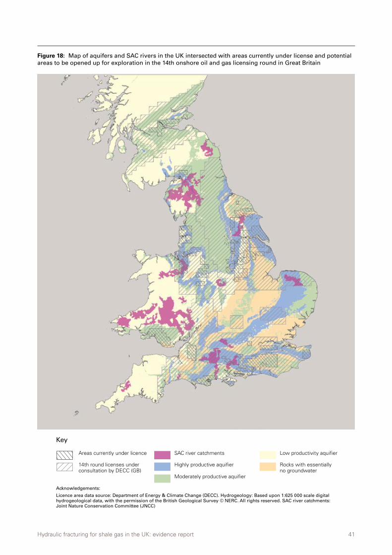
Hydraulic fracturing for shale gas in the UK: evidence report 41
Figure 18: Map of aquifers and SAC rivers in the UK intersected with areas currently under license and potential areas to be opened up for exploration in the 14th onshore oil and gas licensing round in Great Britain
Key
Areas currently under licence
14th round licenses under consultation by DECC (GB)
Acknowledgements:
Licence area data source: Department of Energy & Climate Change (DECC). Hydrogeology: Based upon 1:625 000 scale digital hydrogeological data, with the permission of the British Geological Survey © NERC. All rights reserved. SAC river catchments: Joint Nature Conservation Committee (JNCC)
Key:
Acknowledgements:
0 6030 Km
E1:3,600,000Scale on A4 paperAreas currently under licence 14th roundlicences under consultation by DECC (GB)
Areas currently under licence and 14th round licences underconsultation by DECC (GB)
Licence area data source: Department of Energy & Climate Change (DECC)
Key:
Acknowledgements:
0 6030 Km
E1:3,600,000Scale on A4 paperAreas currently under licence 14th roundlicences under consultation by DECC (GB)
Areas currently under licence and 14th round licences underconsultation by DECC (GB)
Licence area data source: Department of Energy & Climate Change (DECC)
SAC river catchments
Highly productive aquifier
Moderately productive aquifier
Low productivity aquifier
Rocks with essentially no groundwater
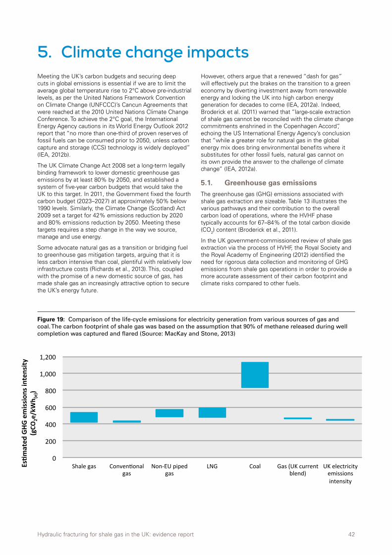
Hydraulic fracturing for shale gas in the UK: evidence report 42
5. Climate change impacts Meeting the UK’s carbon budgets and securing deep cuts in global emissions is essential if we are to limit the average global temperature rise to 2°C above pre-industrial levels, as per the United Nations Framework Convention on Climate Change (UNFCCC)’s Cancun Agreements that were reached at the 2010 United Nations Climate Change Conference. To achieve the 2°C goal, the International Energy Agency cautions in its World Energy Outlook 2012 report that “no more than one-third of proven reserves of fossil fuels can be consumed prior to 2050, unless carbon capture and storage (CCS) technology is widely deployed” (IEA, 2012b).
The UK Climate Change Act 2008 set a long-term legally binding framework to lower domestic greenhouse gas emissions by at least 80% by 2050, and established a system of five-year carbon budgets that would take the UK to this target. In 2011, the Government fixed the fourth carbon budget (2023–2027) at approximately 50% below 1990 levels. Similarly, the Climate Change (Scotland) Act 2009 set a target for 42% emissions reduction by 2020 and 80% emissions reduction by 2050. Meeting these targets requires a step change in the way we source, manage and use energy.
Some advocate natural gas as a transition or bridging fuel to greenhouse gas mitigation targets, arguing that it is less carbon intensive than coal, plentiful with relatively low infrastructure costs (Richards et al., 2013). This, coupled with the promise of a new domestic source of gas, has made shale gas an increasingly attractive option to secure the UK’s energy future.
However, others argue that a renewed “dash for gas” will effectively put the brakes on the transition to a green economy by diverting investment away from renewable energy and locking the UK into high carbon energy generation for decades to come (IEA, 2012a). Indeed, Broderick et al. (2011) warned that “large-scale extraction of shale gas cannot be reconciled with the climate change commitments enshrined in the Copenhagen Accord”, echoing the US International Energy Agency’s conclusion that “while a greater role for natural gas in the global energy mix does bring environmental benefits where it substitutes for other fossil fuels, natural gas cannot on its own provide the answer to the challenge of climate change” (IEA, 2012a).
5.1. Greenhouse gas emissions
The greenhouse gas (GHG) emissions associated with shale gas extraction are sizeable. Table 13 illustrates the various pathways and their contribution to the overall carbon load of operations, where the HVHF phase typically accounts for 67–84% of the total carbon dioxide (CO2) content (Broderick et al., 2011).
In the UK government-commissioned review of shale gas extraction via the process of HVHF, the Royal Society and the Royal Academy of Engineering (2012) identified the need for rigorous data collection and monitoring of GHG emissions from shale gas operations in order to provide a more accurate assessment of their carbon footprint and climate risks compared to other fuels.
Figure 19: Comparison of the life-cycle emissions for electricity generation from various sources of gas and coal. The carbon footprint of shale gas was based on the assumption that 90% of methane released during well completion was captured and flared (Source: MacKay and Stone, 2013)
0
200
400
600
800
1,000
1,200
Shale gas Conven4onal gas
Non-‐EU piped gas
LNG Coal Gas (UK current blend)
UK electricity emissions intensity
Es#m
ated
GHG
emission
s inten
sity
(gCO
2e/kWh (
e))
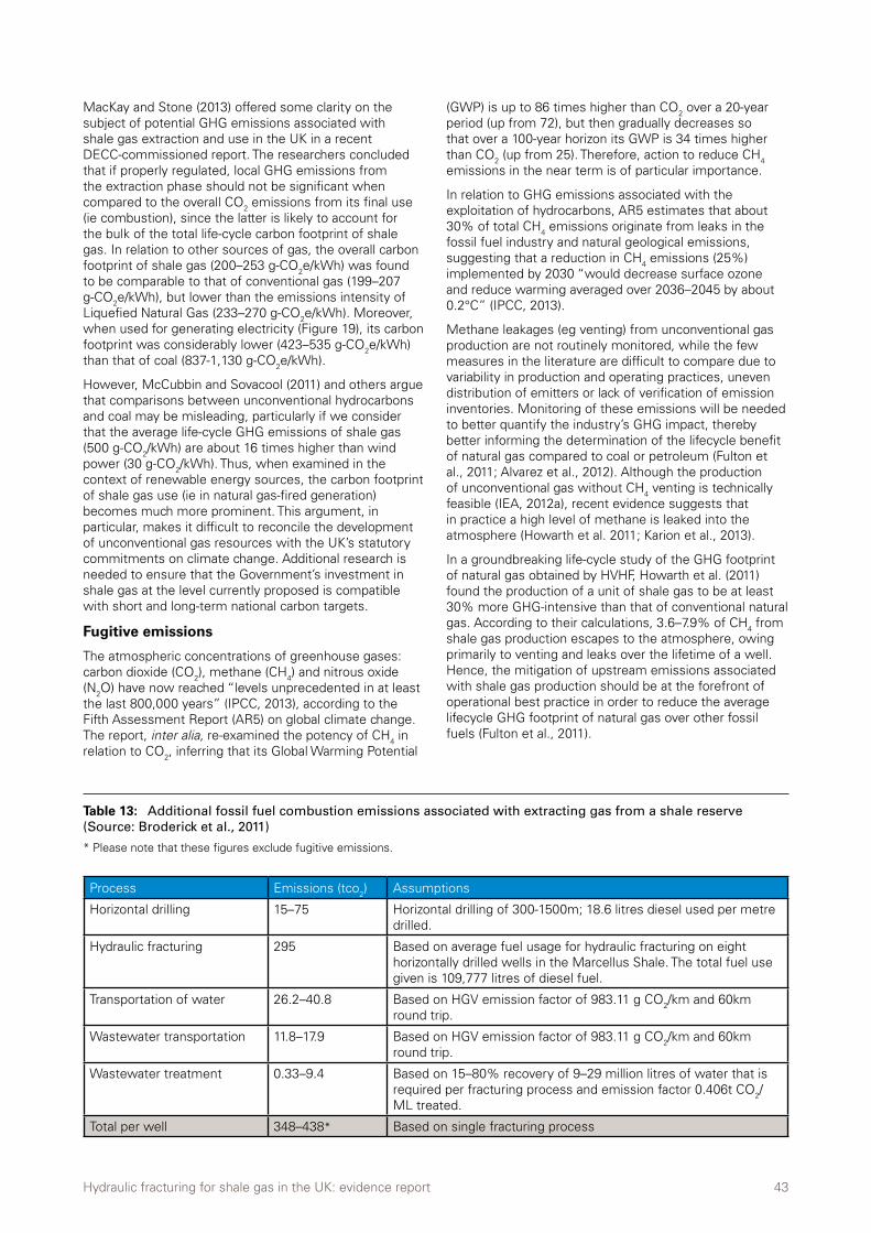
Hydraulic fracturing for shale gas in the UK: evidence report 43
MacKay and Stone (2013) offered some clarity on the subject of potential GHG emissions associated with shale gas extraction and use in the UK in a recent DECC-commissioned report. The researchers concluded that if properly regulated, local GHG emissions from the extraction phase should not be significant when compared to the overall CO2 emissions from its final use (ie combustion), since the latter is likely to account for the bulk of the total life-cycle carbon footprint of shale gas. In relation to other sources of gas, the overall carbon footprint of shale gas (200–253 g-CO2e/kWh) was found to be comparable to that of conventional gas (199–207 g-CO2e/kWh), but lower than the emissions intensity of Liquefied Natural Gas (233–270 g-CO2e/kWh). Moreover, when used for generating electricity (Figure 19), its carbon footprint was considerably lower (423–535 g-CO2e/kWh) than that of coal (837-1,130 g-CO2e/kWh).
However, McCubbin and Sovacool (2011) and others argue that comparisons between unconventional hydrocarbons and coal may be misleading, particularly if we consider that the average life-cycle GHG emissions of shale gas (500 g-CO2/kWh) are about 16 times higher than wind power (30 g-CO2/kWh). Thus, when examined in the context of renewable energy sources, the carbon footprint of shale gas use (ie in natural gas-fired generation) becomes much more prominent. This argument, in particular, makes it difficult to reconcile the development of unconventional gas resources with the UK’s statutory commitments on climate change. Additional research is needed to ensure that the Government’s investment in shale gas at the level currently proposed is compatible with short and long-term national carbon targets.
Fugitive emissions
The atmospheric concentrations of greenhouse gases: carbon dioxide (CO2), methane (CH4) and nitrous oxide (N2O) have now reached “levels unprecedented in at least the last 800,000 years” (IPCC, 2013), according to the Fifth Assessment Report (AR5) on global climate change. The report, inter alia, re-examined the potency of CH4 in relation to CO2, inferring that its Global Warming Potential
(GWP) is up to 86 times higher than CO2 over a 20-year period (up from 72), but then gradually decreases so that over a 100-year horizon its GWP is 34 times higher than CO2 (up from 25). Therefore, action to reduce CH4 emissions in the near term is of particular importance.
In relation to GHG emissions associated with the exploitation of hydrocarbons, AR5 estimates that about 30% of total CH4 emissions originate from leaks in the fossil fuel industry and natural geological emissions, suggesting that a reduction in CH4 emissions (25%) implemented by 2030 “would decrease surface ozone and reduce warming averaged over 2036–2045 by about 0.2°C” (IPCC, 2013).
Methane leakages (eg venting) from unconventional gas production are not routinely monitored, while the few measures in the literature are difficult to compare due to variability in production and operating practices, uneven distribution of emitters or lack of verification of emission inventories. Monitoring of these emissions will be needed to better quantify the industry’s GHG impact, thereby better informing the determination of the lifecycle benefit of natural gas compared to coal or petroleum (Fulton et al., 2011; Alvarez et al., 2012). Although the production of unconventional gas without CH4 venting is technically feasible (IEA, 2012a), recent evidence suggests that in practice a high level of methane is leaked into the atmosphere (Howarth et al. 2011; Karion et al., 2013).
In a groundbreaking life-cycle study of the GHG footprint of natural gas obtained by HVHF, Howarth et al. (2011) found the production of a unit of shale gas to be at least 30% more GHG-intensive than that of conventional natural gas. According to their calculations, 3.6–7.9% of CH4 from shale gas production escapes to the atmosphere, owing primarily to venting and leaks over the lifetime of a well. Hence, the mitigation of upstream emissions associated with shale gas production should be at the forefront of operational best practice in order to reduce the average lifecycle GHG footprint of natural gas over other fossil fuels (Fulton et al., 2011).
Process Emissions (tco2) Assumptions
Horizontal drilling 15–75 Horizontal drilling of 300-1500m; 18.6 litres diesel used per metre drilled.
Hydraulic fracturing 295 Based on average fuel usage for hydraulic fracturing on eight horizontally drilled wells in the Marcellus Shale. The total fuel use given is 109,777 litres of diesel fuel.
Transportation of water 26.2–40.8 Based on HGV emission factor of 983.11 g CO2/km and 60km round trip.
Wastewater transportation 11.8–17.9 Based on HGV emission factor of 983.11 g CO2/km and 60km round trip.
Wastewater treatment 0.33–9.4 Based on 15–80% recovery of 9–29 million litres of water that is required per fracturing process and emission factor 0.406t CO2/ML treated.
Total per well 348–438* Based on single fracturing process
Table 13: Additional fossil fuel combustion emissions associated with extracting gas from a shale reserve (Source: Broderick et al., 2011)
* Please note that these figures exclude fugitive emissions.
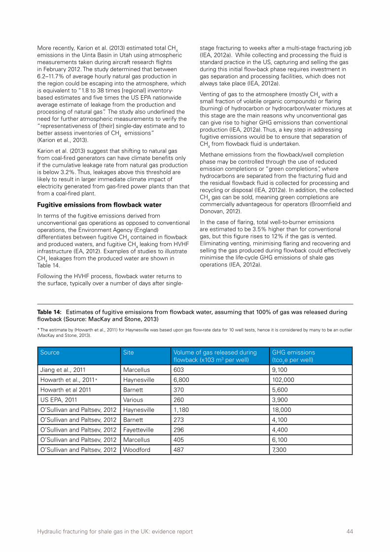
Hydraulic fracturing for shale gas in the UK: evidence report 44
More recently, Karion et al. (2013) estimated total CH4 emissions in the Uinta Basin in Utah using atmospheric measurements taken during aircraft research flights in February 2012. The study determined that between 6.2–11.7% of average hourly natural gas production in the region could be escaping into the atmosphere, which is equivalent to “1.8 to 38 times [regional] inventory-based estimates and five times the US EPA nationwide average estimate of leakage from the production and processing of natural gas”. The study also underlined the need for further atmospheric measurements to verify the “representativeness of [their] single-day estimate and to better assess inventories of CH4 emissions” (Karion et al., 2013).
Karion et al. (2013) suggest that shifting to natural gas from coal-fired generators can have climate benefits only if the cumulative leakage rate from natural gas production is below 3.2%. Thus, leakages above this threshold are likely to result in larger immediate climate impact of electricity generated from gas-fired power plants than that from a coal-fired plant.
Fugitive emissions from flowback water
In terms of the fugitive emissions derived from unconventional gas operations as opposed to conventional operations, the Environment Agency (England) differentiates between fugitive CH4 contained in flowback and produced waters, and fugitive CH4 leaking from HVHF infrastructure (EA, 2012). Examples of studies to illustrate CH4 leakages from the produced water are shown in Table 14.
Following the HVHF process, flowback water returns to the surface, typically over a number of days after single-
stage fracturing to weeks after a multi-stage fracturing job (IEA, 2012a). While collecting and processing the fluid is standard practice in the US, capturing and selling the gas during this initial flow-back phase requires investment in gas separation and processing facilities, which does not always take place (IEA, 2012a).
Venting of gas to the atmosphere (mostly CH4 with a small fraction of volatile organic compounds) or flaring (burning) of hydrocarbon or hydrocarbon/water mixtures at this stage are the main reasons why unconventional gas can give rise to higher GHG emissions than conventional production (IEA, 2012a). Thus, a key step in addressing fugitive emissions would be to ensure that separation of CH4 from flowback fluid is undertaken.
Methane emissions from the flowback/well completion phase may be controlled through the use of reduced emission completions or “green completions”, where hydrocarbons are separated from the fracturing fluid and the residual flowback fluid is collected for processing and recycling or disposal (IEA, 2012a). In addition, the collected CH4 gas can be sold, meaning green completions are commercially advantageous for operators (Broomfield and Donovan, 2012).
In the case of flaring, total well-to-burner emissions are estimated to be 3.5% higher than for conventional gas, but this figure rises to 12% if the gas is vented. Eliminating venting, minimising flaring and recovering and selling the gas produced during flowback could effectively minimise the life-cycle GHG emissions of shale gas operations (IEA, 2012a).
Source Site Volume of gas released during flowback (x103 m3 per well)
GHG emissions (tco2e per well)
Jiang et al., 2011 Marcellus 603 9,100
Howarth et al., 2011* Haynesville 6,800 102,000
Howarth et al 2011 Barnett 370 5,600
US EPA, 2011 Various 260 3,900
O’Sullivan and Paltsev, 2012 Haynesville 1,180 18,000
O’Sullivan and Paltsev, 2012 Barnett 273 4,100
O’Sullivan and Paltsev, 2012 Fayetteville 296 4,400
O’Sullivan and Paltsev, 2012 Marcellus 405 6,100
O’Sullivan and Paltsev, 2012 Woodford 487 7,300
Table 14: Estimates of fugitive emissions from flowback water, assuming that 100% of gas was released during flowback (Source: MacKay and Stone, 2013)
* The estimate by (Howarth et al., 2011) for Haynesville was based upon gas flow-rate data for 10 well tests, hence it is considered by many to be an outlier (MacKay and Stone, 2013).
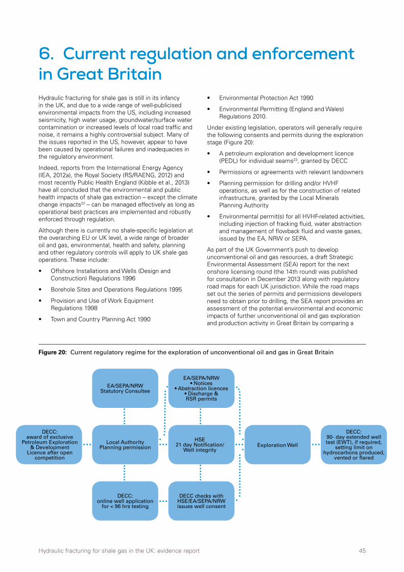
Hydraulic fracturing for shale gas in the UK: evidence report 45
6. Current regulation and enforcement in Great Britain Hydraulic fracturing for shale gas is still in its infancy in the UK, and due to a wide range of well-publicised environmental impacts from the US, including increased seismicity, high water usage, groundwater/surface water contamination or increased levels of local road traffic and noise, it remains a highly controversial subject. Many of the issues reported in the US, however, appear to have been caused by operational failures and inadequacies in the regulatory environment.
Indeed, reports from the International Energy Agency (IEA, 2012a), the Royal Society (RS/RAENG, 2012) and most recently Public Health England (Kibble et al., 2013) have all concluded that the environmental and public health impacts of shale gas extraction – except the climate change impacts22 – can be managed effectively as long as operational best practices are implemented and robustly enforced through regulation.
Although there is currently no shale-specific legislation at the overarching EU or UK level, a wide range of broader oil and gas, environmental, health and safety, planning and other regulatory controls will apply to UK shale gas operations. These include:
• Offshore Installations and Wells (Design and Construction) Regulations 1996
• Borehole Sites and Operations Regulations 1995
• Provision and Use of Work Equipment Regulations 1998
• Town and Country Planning Act 1990
• Environmental Protection Act 1990
• Environmental Permitting (England and Wales) Regulations 2010.
Under existing legislation, operators will generally require the following consents and permits during the exploration stage (Figure 20):
• A petroleum exploration and development licence (PEDL) for individual seams23, granted by DECC
• Permissions or agreements with relevant landowners
• Planning permission for drilling and/or HVHF operations, as well as for the construction of related infrastructure, granted by the Local Minerals Planning Authority
• Environmental permit(s) for all HVHF-related activities, including injection of fracking fluid, water abstraction and management of flowback fluid and waste gases, issued by the EA, NRW or SEPA.
As part of the UK Government’s push to develop unconventional oil and gas resources, a draft Strategic Environmental Assessment (SEA) report for the next onshore licensing round (the 14th round) was published for consultation in December 2013 along with regulatory road maps for each UK jurisdiction. While the road maps set out the series of permits and permissions developers need to obtain prior to drilling, the SEA report provides an assessment of the potential environmental and economic impacts of further unconventional oil and gas exploration and production activity in Great Britain by comparing a
Figure 20: Current regulatory regime for the exploration of unconventional oil and gas in Great Britain
DECC: award of exclusive
Petroleum Exploration & Development
Licence after open competition
Local Authority Planning permission
HSE 21 day Notification/
Well integrityExploration Well
DECC: 90- day extended well test (EWT), if required,
setting limit on hydrocarbons produced,
vented or flared
EA/SEPA/NRW Statutory Consultee
DECC: online well application
for < 96 hrs testing
EA/SEPA/NRW• Notices
• Abstraction licences• Discharge & RSR permits
DECC checks with HSE/EA/SEPA/NRW issues well consent
Hydraulic fracturing for shale gas in the UK: evidence report 46
“low activity” and “high activity” scenario (AMEC, 2013). SEA estimates for the number of wells/well pads are listed in Section 4.
Additional guidance, intended to address the unique aspects of shale gas wells and HVHF operations during the exploration phase, is provided in the form of voluntary guidelines produced by the DECC’s UK Onshore Operators Group (UKOOG). These cover a wide range of issues such as groundwater isolation and protection, fracturing containment, seismicity mitigation, pollution control, water use and waste management (UKOOG, 2013), aiming to foster best practice in the industry. It is important to note, however, that the guidelines are not binding legal obligations – in spite of the input of DECC, HSE, EA and SEPA.
In England, the EA has issued and consulted on draft technical guidance for onshore oil and gas exploratory operations, according to which a mining waste permit will be required for drill cuttings, spent drilling muds and drill fluids, flowback fluids, waste gases and wastes left underground. A permit will also be needed for the flaring of large quantities of waste gas and for groundwater activities, depending on the local hydrology (EA, 2013b).
In Scotland, a license for individual wellheads will be required from SEPA under the Controlled Activities Regulation (CAR)24 (SEPA, 2012). However, SEPA propose that HVHF activities may fall within a WFD exemption, which could allow the discharge of pollutants to the water environment. The regulator intends to assess proposals on an individual basis to determine whether this exemption should apply. SEPA expects application for authorisation to be accompanied by a risk assessment of potential impacts on groundwater and other parts of the water environment, with proposals for appropriate mitigation measures and long-term monitoring.
At present, an Environmental Impact Assessment (EIA) is only required by the Mineral Planning Authority if the oil and gas exploratory drilling operations fall within the schedule 2 threshold 25, and are deemed likely to have significant environmental impacts based on the screening criteria as per schedule 3. The schedule 2 threshold has not yet been applied to any of the pilot developments for shale gas in the UK since none of the well pads exceeded one hectare in size. In October 2013, the European Parliament adopted proposed amendments to the EIA Directive (2011/92/EU), which included an automatic requirement for an impact assessment for the exploration or extraction of shale gas involving hydraulic fracturing, regardless of the amount extracted. Under the existing directive, an EIA is only required when the extraction of natural gas exceeds 500,000 m3 per day. After a fourth round of negotiations in December 2013,
however, the proposal to amend Annex I and mandate EIA for all unconventional oil and gas extraction projects was withdrawn by the Member States. The current agreement is yet to be approved by the European Parliament at a plenary session in early 2014.
In terms of the wider EU context, European countries are adopting a range of approaches to the potential exploitation of shale gas resources, from the pro-development policies of Poland and the UK to the restrictions imposed by France and Bulgaria. In January 2014, the European Commission adopted a series of non-binding recommendations aiming to ensure that proper environmental and climate safeguards are in place for HVHF used in shale gas operations (EC, 2014). Intended to complement existing EU legislation, the recommendations call for Member States to adopt minimum principles within six months of the guidance’s publication and to report to the Commission annually about measures taken. The principles cover a range of issues, such as strategic environmental assessments and planning, underground risk assessment, well integrity, baseline reporting and operational monitoring, capture of methane emissions and disclosure of chemicals used in each well.
6.1. Environmental monitoring
Undoubtedly, one of the most crucial elements of an effective regulatory regime is independent environmental monitoring using the best available techniques. Continuous monitoring of ground gas, for example, is required to identify potential leakages of methane and other emissions before, during and after shale gas operations (RS/RAENG, 2012) in order to provide robust evidence that on-site environmental controls are working and no environmental hazards associated with fugitive methane has occurred (Talbot and Morris, 2012).
We have already established that the regulatory framework that applies to shale gas in the UK is, in effect, the same as for conventional oil and gas extraction. Current safeguards are too reliant on self inspection, and on the HSE who may not have the specialised knowledge to identify malpractice that may impact on groundwater. Cuadrilla were not required to have an environmental permit for discharge to groundwater for their site at “Preese Hall”, which would have brought them under an appropriate regulatory regime for groundwater protection, because this was not considered to be a risk under “normal operating conditions”. This approach seems to overlook the risks of failure (of integrity of the wells), however low these risks may be, and is inconsistent with the approach taken to other activities, such as landfill operations, which do require a permit.
22 It is worth noting that climate change impacts can be improved through capturing of fugitive emissions and methane in flowback water, greatly improving the GHG budget.
23 An individual consent covers rights for multiple wellheads on one seam; the consent issued to Cuadrilla for Bowland shale, for instance, could cover between 190 and 810 wellheads, each approximately 1 ha in size.
24 The Water Environment (Controlled Activities) (Scotland) Regulations 2011, commonly known as the Controlled Activity Regulations (CAR), regulates activities (eg, abstraction, pollution control, groundwater, impoundment) associated with the Scottish water environment. Authorisations for these types of activities are assessed and granted by SEPA.
25 Town and Country Planning (Environmental Impact Assessment) Regulations 2011.
Hydraulic fracturing for shale gas in the UK: evidence report 47
Much of the discussion to date on European shale gas development has been driven by events occurring in the United States, especially by incidents where industry did not employ best practice.
There are a considerable number of potential risks to the natural environment associated with commercial shale exploration and production in the UK because of the disturbance to wildlife and the land take of the infrastructure itself, interactions with the water environment, and the release of greenhouse gas emissions to the atmosphere during the extraction process and use of the gas. These risks can partly be addressed through an improved regulatory regime, but there remains considerable uncertainty as to whether the commercial extraction of shale gas in the UK is compatible with the UK Government’s climate change objectives.
All activities associated with unconventional gas exploration and production in the UK are covered by existing EU and national environmental legislation. Our analysis suggests that the current regulatory regime is not fit for purpose and therefore unable to adequately manage serious environmental risks that may arise from individual projects and cumulative developments, such as species disturbance, water stress and inevitably the residual risk around pollution. Additionally, there is a significant risk that taxpayers and third parties could be forced to pick up liability for damage caused.
Through detailed analysis, the report identified the following three categories of key environmental risk:
(i) Risk to the water environment
(ii) Risk of ecological impacts
(iii) Risk of climate change impacts
(i) Risk to the water environment
Water management has emerged as a critical issue in the development of shale gas resources. This is due to the large volumes of water and chemicals required for the drilling and hydraulic fracturing of multiple wells, which inevitably lead to the production of significant quantities of wastewater that must be managed and disposed of safely and with due diligence. A recent AMEC report has estimated that under the high activity scenario the water use of the UK shale gas industry could amount to 9 million m3 per year, which would represent around 18% of mains water currently supplied to the energy, water and waste sectors. Additionally, under the same scenario up to 108 million m3 of wastewater would require treatment26, which would place a significant burden on the existing wastewater treatment infrastructure (AMEC, 2013).
Another issue is the historic over-allocation of abstraction licences, which could mean that significant additional demand for water resources could exacerbate pressure
on rivers and wetlands from the public water supply. Particularly sensitive water bodies, and those already suffering from over abstraction, such as chalk streams could be especially at risk.
As with all drilling operations, spills, blowouts and equipment failures are issues that must be effectively managed and mitigated. The release of methane during hydraulic fracturing can result in groundwater contamination. Induced seismic events can potentially undermine the integrity of wells and their casing. The potential impacts of hydraulic fracturing, especially with regard to groundwater, are significant and potentially long lasting or even irreversible.
(ii) Risk of ecological impacts
Habitat loss, fragmentation and disturbance are likely to be the main impacts on wildlife, aside from the risks of pollution of habitats and water bodies.
With each well pad occupying up to 3 hectares and with up to 120 well pads being constructed and linked by infrastructure in the UK over the next two decades, under the high activity scenario (AMEC, 2013), if well pads are sited in the wrong place and/or constructed at the wrong time of year impacts could be very damaging to important and protected species. Site selection will be a key factor in minimising impacts on species and habitats. Our analysis, for instance, found that around 4% of areas under consultation in the 14th licensing round will coincide with land under Special Protection Area designation and over 13% will overlay Areas of Outstanding Natural Beauty.
The drilling and hydraulic fracturing process can be a 24-hour/7-day per week operation with associated visual and noise impacts. Disturbance from drilling can be compounded by hundreds of truck movements required to transport equipment and wastes, including flowback and produced wastewaters contaminated with highly-saline mineral compounds and naturally occurring radioactive materials. Light pollution could have serious ecological consequences for a range of species, including invertebrates and bats.
(iii) Risk of climate change impacts
The exploitation of shale gas must be seen within the context of the UK’s legally binding commitments to achieve an 80% reduction in greenhouse gas emissions by 2050. Not only does a “dash for gas” risk diverting funding and resources from the expansion of renewable energy technologies, but there is an ongoing debate about the relative leakage rate of methane into the atmosphere from the exploitation of shale gas in comparison to the emission rate from conventional gas. This is potentially important because a high leakage rate of methane might mean that the net greenhouse gas footprint of shale gas could be higher than that of coal, for instance.
Conclusion
26 This reflects cumulative volume for up to 120 well pads over a 20-year period.
Hydraulic fracturing for shale gas in the UK: evidence report 48
ADAMS, M.B. (2011) Land application of hydrofracturing fluids damages a deciduous forest stand in West Virginia. Journal of Environmental Quality, 40: 1340–1344.
ALVAREZ, R.A., PACALA, S.W., WINEBRAKE, J.J., CHAMEIDES, W.L. and HAMBURG, S.P. (2012) Greater focus needed on methane leakage from natural gas infrastructure. PNAS, doi: 10.1073/pnas.1202407109.
AMEC (2013) Strategic Environmental Assessment for further onshore oil and gas licensing: environmental report. Prepared for the Department of Energy and Climate Change. London, UK: AMEC Environment and Infrastructure UK Ltd.
ANDREWS, I.J. (2013) The Carboniferous Bowland Shale gas study: geology and resource estimation. London, UK: British Geological Survey for Department of Energy and Climate Change.
APLIN, A. (2014) From UK Resources to Reserves: What is Required? Durham Energy Institute, Department of Earth Sciences. Presented at the Shale Gas UK 2014 conference, London, 4 March 2014.
BAMBERGER, M. and OSWALD, R.E. (2012) Impacts of gas drilling on human and animal health. New Solutions, 22 (1): 51–77.
BARBER, J.R., BURDETT, C.L., REED, S.E., WARNER, K.A., FORMICHELLA, C., CROOKS, K.R., THEOBALD, D.M. and FRISTRUP, K.M. (2011) Anthropogenic noise exposure in protected natural areas: estimating the scale of ecological consequences. Landscape Ecology, 26 (9): 1281–1295.
BARBER, J.R., CROOKS, K.R. and FRISTRUP, K.M. (2009) The costs of chronic noise exposure for terrestrial organisms. Trends in Ecology and Evolution, 25 (3), 180–189.
BEGOS, K. (2013) DOE study: Fracking chemicals didn’t taint water. Associated Press [online]. Available at: <http://goo.gl/gMIJlw>. [Accessed 28 Aug 2013].
BGS (2012) The Unconventional Hydrocarbon Resources of Britain’s Onshore Basins – Shale Gas. London, UK: British Geological Survey for the Department of Energy and Climate Change.
BLOOMFIELD, M. (2012) Support to the identification of potential risks for the environment and human health arising from hydrocarbons operations involving hydraulic fracturing in Europe (report for European Commission DG Environment). Didcot, UK: AEA Technology plc.
BNEF (2013) Shale gas exploitation unlikely to bring down UK electricity bills. Bloomberg New Energy Finance [online]. Available at: <http://goo.gl/R4VJxV>. [Accessed 04 Oct 2013].
BOLDOGH, S., DOBROSI, D. and SAMU, P. (2007) The effects of the illumination of buildings on house-dwelling bats and its conservation consequences. Acta Chiropterologica, 9 (2): 527–534.
BRIGHT, J., LANGSTON, R., BULLMAN, R., EVANS, R., GARDNER, S. and PEARCE-HIGGINS, J. (2008) Map of bird sensitivities to wind farms in Scotland: A tool to aid planning and conservation. Biological Conservation, 141: 2342–56.
BRIGHT, J., LANGSTON, R.H.W and ANTHONY, S. (2009) Mapped and written guidance in relation to birds and onshore wind energy development in England. RSPB research report no. 35. Sandy, UK: The RSPB.
BRIGHT, J.A., LANGSTON, R.H.W., BULLMAN, R., EVANS, R.J., GARDNER, S., PEARCE-HIGGINS, J and WILSON, E. (2006) Bird sensitivity map to provide locational guidance for onshore wind farms in Scotland. RSPB research report no. 20. Sandy, UK: The RSPB.
BRODERICK. J., ANDERSON, K., WOOD, R., GILBERT, P, SHARMINA, M., FOOTITT, A., GLYNN, S. and NICHOLLS, F. (2011) Shale gas: an updated assessment of environmental and climate change impacts. Manchester, UK: Tyndall Centre for Climate Change Research, University of Manchester.
BROOMFIELD, M. and DONOVAN, B. (2012) Monitoring and control of fugitive methane from unconventional gas operations. Bristol, UK: Environment Agency.
BRUCE-WHITE, C. and SHARDLOW, M. (2011) A review of the impact of artificial light on invertebrates: Putting the backbone into invertebrate conservation. Peterborough, UK: Buglife – The Invertebrate Conservation Trust.
BRUMM, H. (2004) The impact of environmental noise on song amplitude in a territorial bird. Journal of Animal Ecology, 73(3): 434–440.
CALL, M. ( 1979) Habitat Management Guides for Birds of Prey. Technical Note, US Department of the Interior- Bureau of Land Management.
CARNEY, K.M. and SYDEMAN, W.J. (1999) A Review of Human Disturbance Effects on Nesting Colonial Waterbirds, International Journal of Waterbird Biology, 22: 68–79.
References
Hydraulic fracturing for shale gas in the UK: evidence report 49
COOLEY, H. and DONNELLY, K. (2012) Hydraulic Fracturing and Water Resources: Separating the Frack from the Fiction. Oakland, California: Pacific Institute.
CPRE (2003) Night blight. London: Campaign to Protect Rural England.
CUADRILLA (2013) Fracturing Fluid [online]. Available at: <http://goo.gl/s7JFA6>. [Accessed 12 Aug 2013].
CURRIE, F. and ELLIOT, G. (1997) A guide to managing forests for rare birds. The Forest Authority and The RSPB, UK.
DAVIES, R., FOULGER, G., BINDLEY, A. and STYLES, P. (2013) Induced seismicity and hydraulic fracturing for the recovery of hydrocarbons, Marine and Petroleum Geology, 45: 171–185.
DAVIES, R.J., MATHIAS,S., MOSS, J., HUSTOFT, S. and NEWPORT, L. (2012) Hydraulic fractures: How far can they go? Marine and Petroleum Geology, 37 (1): 1–6, doi: 10.1016/j.marpetgeo.2012.04.001.
DCLG (2013) Planning practice guidance for onshore oil and gas. London, UK: Department for Communities and Local Government.
DE PATER, C.J. and BAISCH, S. (2011) Geomechanical Study of Bowland Shale Seismicity: Synthesis Report. Lichfield, UK: Cuadrilla Resources Ltd.
DEFRA (2013) Statistical data set: ENV15 – Water abstraction tables [online]. Available at: <http://goo.gl/WkjXVg> [Accessed 27 Nov 2013].
DOW (2013) Recycle of Produced and Flowback Water in Eagle Ford Shale Texas Picks up Momentum with Omni Water Solutions and Dow Water and Process Solutions [online]. Available at: <http://goo.gl/QnpUeI> [Accessed 05 Feb 2013].
DROHAN, P.J., BRITTINGHAM, M., BISHOP, J. and YODER, K. (2012) Early trends in landcover change and forest fragmentation due to shale-gas development in Pennsylvania: a potential outcome for the Northcentral Appalachians. Environmental Management, 49 (5): 1061–75. doi: 10.1007/s00267-012-9841-6.
EA and NRW (2013) Water stressed areas – final classification. Developed by the Environment Agency and Natural Resources Wales.
EA (2008) Water resources in England and Wales – current state and future pressures. Bristol, UK: Environment Agency.
EA (2009) Water for people and the environment: Water Resources Strategy for England and Wales. Bristol, UK: Environment Agency.
EA (2011) Shale Gas: North West – Monitoring of Flowback water. Bristol/ London, UK: Environment Agency.
EA (2012) Monitoring and control of fugitive methane from unconventional gas operations. Bristol/ London, UK: Environment Agency.
EA (2013a) Managing water abstraction (LIT 4892 / 746_12 Version 3). Bristol, UK: Environment Agency.
EA (2013b) Onshore oil and gas exploratory operations: technical guidance, Consultation Draft, August 2013. Bristol, UK: Environment Agency.
EA (2013c) Lune and Wyre abstraction licensing strategy. Bristol, UK: Environment Agency.
EC (2014) Commission recommendation on minimum principles for the exploration and production of hydrocarbons (such as shale gas) using high volume hydraulic fracturing – C(2014) 267 /3. Brussels, Belgium: European Commission.
EEA (2008) Water scarcity – European Environment Agency (EEA) [online]. Available at: <http://www.eea.europa.eu/themes/water/featured-articles/water-scarcity> [Accessed 23 Jan 2014].
EIA (2013) Technically Recoverable Shale Oil and Shale Gas Resources: An Assessment of 137 Shale Formations in 41 Countries outside the United States. Washington, DC, US: US Energy Information Administration.
ENS (2011) Toxic Diesel Fuel Used Without Permits in Fracking Operations. Environmental News Service [online]. Available at: <http://goo.gl/FaoLN3>. [Accessed 12 Aug 2013].
ENTREKIN,S., EVANS-WHITE, M., JOHNSON, B. and HAGENBUCH, E. (2011) Rapid expansion of natural gas development poses a threat to surface waters. Frontiers in Ecology and the Environment, 9(9): 503–511, DOI: 10.1890/110053.
FAHRIG, L. (2003) Effects of Habitat Fragmentation on Biodiversity. Annual Review of Ecology, Evolution and Systematics, 34: 487–515.
FISHER, K. (2010) Data Confirm Safety Of Well Fracturing. Derby, Kansas, US: The American Oil and Gas Reporter.
FISHER, M. (2012) Fracking’s Footprint: Scientists Study Impact of Shale Gas Development on Pennsylvania’s Forests. CSA News, July 2012: 4–11.

Hydraulic fracturing for shale gas in the UK: evidence report 50
FONTENOT, B.E., HUNT, L.R., HILDENBRAND, Z.L., CARLTON JR., D.D., OKA,H., WALTON, J.L., HOPKINS, D., OSORIO, A., BJORNDAL, B., HU, Q.H. and SCHUG, K.A. (2013) An Evaluation of Water Quality in Private Drinking Water Wells Near Natural Gas Extraction Sites in the Barnett Shale Formation. Environ. Sci. Technol., doi: 10.1021/es4011724.
FORESTRY COMMISSION (2006) FCS Guidance Note 32: Forest operations and birds in Scottish forests. Scotland, UK: Forestry Commission.
FREYMAN, M. and SALMON, R. (2013) Hydraulic fracturing and Water Stress: Growing Competitive Pressures on Water. Boston, MA, US: Ceres.
FULTON, M., MELLQUIST, N., KITASEI, S. and BLUESTEIN, J. (2011) Comparing life-cycle greenhouse gas emissions from natural gas and coal. DB Climate Change Advisors in collaboration with Worldwatch Institute.
GILL, J.A., NORRIS, K. and SUTHERLAND, W.J. (2001) The effects of disturbance on habitat use by black-tailed godwits Limosa limosa. Journal of applied Ecology, 38: 846–856.
GILL, J.A., SUTHERLAND, W.J. and ATKINSON, A.R. (1996) A method to quantify the effects of human disturbance on animal populations. Journal of applied Ecology, 33: 786–792.
GILLEN, J.L. and KIVIAT, E. (2012) Hydraulic Fracturing Threats to Species with Restricted Geographic Ranges in the Eastern United States. Environmental Practice, 14: 320–331. doi: 10.1017/S1466046612000361.
GOV.UK (2013a) Harnessing the potential of the UK’s natural resources: a fiscal regime for shale gas [online]. Available at: <http://goo.gl/VQ9AgI>. [Accessed 04 Feb 2014].
GOV.UK (2013b) Oil and gas: petroleum licensing guidance – Detailed guidance [online]. Available at: <http://goo.gl/JEzOvy>. [Accessed 04 Oct 2013].
GRAYLING, T. (2012) Regulation of shale gas extraction in Great Britain, Geological Society briefing, London, 18 June 2012. London, UK: Environment Agency.
GREEN, C.A., STYLES, P. and BAPTIE, B.J. (2012) Preese Hall shale gas fracturing review and recommendations for induced seismic mitigation. London, UK: Department of Energy and Climate Change.
GREENAWAY, F. (2008) Barbastelle Bats in the Sussex West Weald 1997–2008 [unpublished]. Available at: <http://goo.gl/CZbDfn>. [Accessed 10 Dec 2013].
GREGORY, K.B., VIDIC, R.D. and DZOMBAK, D.A. (2011) Water management challenges associated with the production of shale gas by hydraulic fracturing. Elements, 7(3):181–186
GROAT, C.G. and GRIMSHAW, T.W. (2012) Fact-Based Regulation for Environmental Protection in Shale Gas Development: Summary of Findings. Austin, Texas, US: The Energy Institute, University of Texas.
HEALY, D. (2012) Hydraulic Fracturing or “Fracking”: A Short Summary of Current Knowledge and Potential Environmental Impacts. A Small Scale Study for the Environmental Protection Agency (Ireland) under the Science, Technology, Research and Innovation for the Environment (STRIVE) Programme 2007–2013. Aberdeen, UK: University of Aberdeen.
HOLMES. T.L., KNIGHT ,R.L., HENITS, L. and CRAIG, G.R. (1993) Responses of Wintering Grassland Raptors to Human Disturbance. Wildlife Society Bulletin, 21 (4): 461–468.
HOWARTH, R.W., SANTORO, R. and INGRAFFEA, A. (2011) Methane and the greenhouse-gas footprint of natural gas from shale formations. Climatic Change, 106 (4): 679-690. DOI: 10.1007/s10584-011-0061-5.
HOWORTH, R. (2009) Field Survey of Barbastelle Bat Flightlines’ Condition from Ebernoe SAC 2008 [unpublished]. Available at: <http://goo.gl/m7hlXk>. [Accessed 10 Dec 2013].
HUGHES, J.D. (2013) Drill, Baby, Drill: Can Unconventional Fuels Usher in a New Era of Energy Abundance? Santa Rosa, California, US: Post Carbon Institute.
IEA (2012a) Golden Rules for a Golden Age of Gas: World Energy Outlook Special Report on Unconventional Gas. Paris, France: International Energy Agency (IEA).
IEA (2012b) World Energy Outlook 2012: Executive Summary. Paris, France: International Energy Agency (IEA).
IPCC (2013) Climate Change 2013: The Physical Science Basis. Working Group I Contribution to the IPCC Fifth Assessment Report. Bern, Switzerland: IPCC Working Group I.
JACKSON, R.B., VENGOSH, A., DARRAH, T.H., WARNER, N.R., DOWN, A., POREDA, R.J., OSBORN, S.G., ZHAO, K. and KARR, J.D. (2013) Increased stray gas abundance in a subset of drinking water wells near Marcellus shale gas extraction. PNAS, doi: 10.1073/pnas.1221635110.
JIANG, M., GRIFFIN, W.M., HENDRICKSON, C., JARAMILLO, P., VANBRIESEN, J. and VENKATESH, A. (2011) Life cycle greenhouse gas emissions of Marcellus Shale gas, Environmental Research Letters, 6(034014), doi: 10.1088/1748-9326/6/3/034014.
Hydraulic fracturing for shale gas in the UK: evidence report 51
JOHNSON, N, GAGNOLET, T, RALLS, R, ZIMMERMAN, E, EICHELBERGER, B, TRACEY, C, KREITLER, G, ORNDORFF, S, TOMLINSON, J, BEARER, S and SARGENT, S. (2010) Pennsylvania Energy Impacts Assessment – Report 1: Marcellus Shale Natural Gas and Wind. Harrisburg, PA, US: The Nature Conservancy - Pennsylvania Chapter.
KAISER, M.J., GALANIDI, M., SHOWLER, D.A., ELLIOTT, A.J., CALDOW, R.W.G., REES, E.I.S., STILLMAN, R.A. and SUTHERLAND, W.J. (2006) Distribution and behaviour of Common Scoter Melanitta nigra relative to prey resources and environmental parameters, Ibis, 148: 110–128.
KARION, A., SWEENEY, C., PÉTRON, G., FROST, G., MICHAEL HARDESTY, R., KOFLER, J., MILLER, B.R., NEWBERGER, T., WOLTER, S., BANTA, R., BREWER, A., DLUGOKENCKY, E., LANG, P., MONTZKA, S.A., SCHNELL, R., TANS, P., TRAINER, M., ZAMORA, R. and CONLEY, S. (2013) Methane emissions estimate from airborne measurements over a western United States natural gas field. Geophysical Research Letters, doi: 10.1002/grl.50811.
KASELOO, P.A. (2005) Synthesis of noise effects on wildlife populations. In Proceeding of the International Conference on Ecology and Transportation, North Carolina State University, Raleigh, NC, 33–35.
KEISTER, T. (2010) Marcellus Hydrofracture Flowback and Production Wastewater Treatment, Recycle, and Disposal Technologies [online]. Available at: <http://goo.gl/ySw9Lb> [Accessed 05 Feb 2013].
KENDALL, R., SMITH, N. and BLOODWORTH, A. (2011) Mineral Planning Factsheet: Alternative Fossil Fuels. London, UK: British Geological Survey for the Department for Communities and Local Government.
KIBBLE, A., CABIANCA, T., DARAKTCHIEVA, Z., GOODING, T., SMITHARD, J., KOWALCZYK, G., MCCOLL, N.P., SINGH, M., VARDOULAKIS, S. and KAMANYIRE, R. (2013) Review of the Potential Public Health Impacts of Exposures to Chemical and Radioactive Pollutants as a Result of Shale Gas Extraction (Draft for Comment, PHE-CRCE-002). London, UK: Public Health England.
KIM, W.-Y. (2013), Induced seismicity associated with fluid injection into a deep well in Youngstown, Ohio. Journal of Geophysical Research: Solid Earth, 118 (7) 3506–3518, doi: 10.1002/jgrb.50247.
KING, G.E. (2010) Thirty Years of Gas Shale Fracturing: What Have We Learned? SPE 133456. London, UK: Society of Petroleum Engineers.
KIVIAT, E. (2013) Risks to biodiversity from hydraulic fracturing for natural gas in the Marcellus and Utica shales. Annals of the New York Academy of Sciences, 1286 (1): 1–14, doi: 10.1111/nyas.12146.
LANCASHIRE COUNTY COUNCIL (2013) Table of bird disturbance [online] Available at: <http://goo.gl/pqN1Ai> [Accessed 18 Nov 2013].
LANGSTON, R. H. W., DREWITT, A. and LILEY, D. (2007b) Bird conservation and access: coexistence or compromise? British Wildlife, October 2007: 1–9.
LANGSTON, R. H. W., LILEY, D., MURISON, G., WOODFIELD, E. and CLARKE, R. T. (2007a) What effects do walkers and dogs have on the distribution and productivity of breeding European Nightjar Caprimulgus. Ibis, 149: 27–36.
LILEY, D. and CLARKE, R. T. (2003) The impact of urban development and human disturbance on the numbers of nightjars Camprimulgus europaeus on heathlands in Dorset, England. Biological Conservation, 114: 219-230.
LILEY, D. and FEARNLEY, H. (2011) Bird Disturbance Study, North Kent 2010/11. Footprint Ecology, UK.
MACKAY, D.J.C. and STONE, T.J. (2013) Potential Greenhouse Gas Emissions Associated with Shale Gas Extraction and Use. London, UK: Department of Energy and Climate Change.
MAUGERI, L. (2013) The Shale Oil Boom: A US Phenomenon. Discussion Paper 2013–05. Cambridge, MA, US: Belfer Center for Science and International Affairs, Harvard Kennedy School.
MCCUBBIN, D. and SOVACOOL, B. (2011) The hidden Factors That Make Wind Energy Cheaper than Natural Gas in the United States, The Electricity Journal, 24 (9), 84–95.
MIT (2011) The Future of Natural Gas: An Interdisciplinary MIT study. Cambridge, MA, US: Massachusetts Institute of Technology.
MOCKFORD, E.J. and MARSHALL, R.C. (2009) Effects of urban noise on song and response behaviour in great tits. Proceedings of the Royal Society B-Biological Sciences, 276(1669): 2979–2985.
MOORE, S. and LESS, S. (2012) Gas Works? Shale gas and its policy implications. London, UK: Policy Exchange.
MURISON, G. (2002) The impact of human disturbance on the breeding success on nightjar on heathlands in south Dorset, England. English Nature Research Report 483, English Nature Peterborough.
MURPHY, S., HILL, D. and GREENAWAY, F. (2009) Pilot study of a technique for investigating the effects of artificial light and noise on bat activity. Brighton, UK: University of Sussex report for People’s Trust for Endangered Species.
NATIONAL PARK SERVICE– ROCKY MOUNTAIN REGION (1995) Final Climbing Management Pld finding of no significant Impact. US Department of the Interior, DeviI’s Tower National Monument.
Hydraulic fracturing for shale gas in the UK: evidence report 52
NATIONAL RESEARCH COUNCIL (2012) Induced Seismicity Potential in Energy Technologies. Washington, DC, US: The National Academies Press.
NPCA (2013) National Parks and Hydraulic Fracturing: Balancing Energy Needs, Nature, and America’s National Heritage. Washington, D.C., US: NPCA’s Center for Park Research.
NYGAARD, R. (2010) Well Design and Well Integrity: Wabamun Area CO2 Sequestration Project. Institute For Sustainable Energy, Environment And Economy, Calgary, Canada: University of Calgary.
OLMSTEAD, S.M., MUEHLENBACHS, L.A., SHIH, J-S, CHU, Z. and KRUPNICK, A.J. (2013) Shale gas development impacts on surface water quality in Pennsylvania. PNAS, 110 (13): 4962–4967, doi: 10.1073/pnas.1213871110.
OSBORN, S.G., VENGOSH, A., WARNER, N.R. and JACKSON, R.B. (2011) Methane contamination of drinking water accompanying gas-well drilling and hydraulic fracturing. PNAS, 108 (20): 8172–8176, doi:10.1073/pnas.1100682108.
O’SULLIVAN, F. and PALTSEV, S. (2012) Shale Gas Production: Potential versus Actual Greenhouse Gas Emissions, Environmental Research Letters, 7(044030), 1–6.
PAPOULIAS, D.M. and VELASCO, A.L. (2013) Histopathological Analysis of Fish from Acorn Fork Creek, Kentucky, Exposed to Hydraulic Fracturing Fluid Releases. Southeastern Naturalist, 12 (Special Issue 4): 92–111.
PARRIS, K.M. and SCHNEIDER, A. (2009) Impacts of Traffic Noise and Traffic Volume on Birds of Roadside Habitats. Ecology and Society, 14(1): 23.
PLATTEEUW, M. and BEEKMAN, J.H. (1994) Disturbance of waterbirds by ships on lakes Ketelmeer and Ijsselmeer, Limosa, 67: 27–33.
RASSENFOSS, S (2011) From Flowback to Fracturing: Water Recycling Grows in the Marcellus Shale. Journal of Petroleum Technology, July 2011, pp. 48–51.
RCEP (2009) Artificial Light in the Environment. Norwich, UK: The Stationery Office (for the Royal Commission on Environmental Pollution).
REIJNEN, R., FOPPEN, R. and MEEUWSEN, H. (1996) The effects of traffic on the density of breeding birds in Dutch agricultural grasslands. Biological Conservation, 75(3): 255–260.
REIJNEN, R., FOPPEN, R. and VEENBAAS, G. (1997) Disturbance by traffic of breeding birds: Evaluation of the effect and considerations in planning and managing road corridors. Biodiversity and Conservation, 6(4): 567–581.
RICHARDS, P., FELL, M. and SMITH, L. (2013) Shale gas and fracking (Standard Note: SN/SC/6073). London, UK: House of Commons Library.
RS/ RAENG (2012) Shale gas extraction in the UK: a review of hydraulic fracturing. London, UK: The Royal Society/ The Royal Academy of Engineering (RS/RAENG).
RUDDOCK, M. and WHITFIELD, D.P. (2007) A Review of Disturbance Distances in Selected Bird Species. Conducted by Natural Research Ltd. Inverness, UK: Scottish Natural Heritage.
SANTORO, R.L., HOWARTH, R.W. and INGRAFFEA, A.R. (2011) Indirect Emissions of Carbon Dioxide from Marcellus Shale Gas Development. A Technical Report from the Agriculture, Energy and Environment Program at Cornell University. New York, US: Cornell University.
SCHUECK, L.S., MARZLUFF, J.M. and STEENHOF, K. (2001) Influence of military activities on raptor abundance and behavior. Condor, 103(3): 606–615.
SCHWEMMER, P., MENDEL, B., SONNTAG, N., DIERSCHKE, V. AND GARTHE, S. (2011) Effects of ship traffic on seabirds in offshore waters: implications for marine conservation and spatial planning, Ecological Applications, 21: 1851–1860.
SEPA (2012) Regulatory guidance: Coal bed methane and shale gas. Stirling, UK: Scottish Environment Protection Agency (SEPA).
SLONECKER, E.T., MILHEIM, L.E., ROIG-SILVA, C.M., MALIZIA, A.R., MARR, D.A. and FISHER, G.B. (2012) Landscape consequences of natural gas extraction in Bradford and Washington Counties, Pennsylvania, 2004–2010. US Geological Survey, Open-File Report 2012–1154.
SMART, R., WHITE, C.C., TOWNEND, J. and CRESSER, M.S. (2001) A model for predicting chloride concentrations in river water in a relatively unpolluted catchment in north-east Scotland. Science of the Total Environment, 265 (1-3): 131–141.
SNH (2012) Assessing Connectivity with Special Protection Areas (SPAs). UK: Scottish Natural Heritage.
SPELLMAN, F.R. (2013) Environmental Impacts of Hydraulic Fracturing. Boca Raton, FL, US: Taylor and Francis Group, LLC.
Hydraulic fracturing for shale gas in the UK: evidence report 53
STEVENS, P. (2013) Energy, Environment and Resources 2013/02: Shale Gas in the United Kingdom. London, UK: Chatham House.
STONE, E. (2000) Separating the noise from the noise: A finding in support of the “Niche Hypothesis,” that birds are influenced by human-induced noise in natural habitats. Anthrozoos, 13(4): 225–231.
STONE, E.L., JONES, G. and HARRIS, S. (2009) Street Lighting Disturbs Commuting Bats. Current Biology, 19, 1–5.
STONE, E.L., JONES, G. and HARRIS, S. (2012) Conserving energy at a cost to biodiversity? Impacts of LED lighting on bats. Global Change Biology, 18 (8): 2458–2465.
STROUD, D.A., CHAMBERS, D., COOK, S., BUXTON, N., FRASER, B., CLEMENT, P., LEWIS, P., MCLEAN, I., BAKER, H. and WHITEHEAD, S. (2001) The UK SPA network: its scope and content. Peterborough, UK: JNCC.
SWENSON, J.E. (1979) Factors affecting status and reproduction of Ospreys in Yellowstone National Park. Journal of Wildlife Management, 43: 595–601.
TALBOT, S. and MORRIS, P. (2012) UK Shale Gas – The Role of Baseline and Operational Continuous Ground-gas Monitoring. Jointly produced by Ground-Gas Solutions Ltd and Ion Science Ltd.
TALKS, L. (2014) Chalk river briefing. Reading, UK: Environment Agency, South East River Basin Planning and Ecology Team.
TAYLOR, C. and LEWIS, D. (2013) Infrastructure for Business 2013 #6: Getting shale gas working. London, UK: Institute of Directors.
TOPPING, C. and PETERSEN, I.K. (2011) Report on a red-throated diver agent-based model to assess the cumulative impact from offshore wind farms. Report commissioned by Vattenfall A/S. Aarhus University, DCE – Danish Centre for Environment and Energy.
UK PARLIAMENT (2014) The Economic Impact on UK Energy Policy of Shale Gas and Oil [online]. Available at: <http://goo.gl/8QC27y>. [Accessed 04 Feb 2014].
UKOOG (2013) UK Onshore Shale Gas Well Guidelines: Exploration and appraisal phase. London, UK: United Kingdom Onshore Operators Group (UKOOG).
US EPA (2011) Inventory of US Greenhouse Gas Emissions and Sinks. Washington, DC: US Environmental Protection Agency.
US FISH AND WILDLIFE SERVICE (1984) American Peregrine Falcon Rocky Mountain Southwest Population Recovery Plan, United States Fish and Wildlife Service, US.
VAN DAELE, L.J. and VAN DAELE, H.A. (1982) Factors Affecting the Productivity of Ospreys Nesting in West-Central Idaho. Condor, 84: 292–299.
VAN DER ELST, N.J., SAVAGE, H.M., KERANEN, K.M. and ABERS, G.A. (2013) Enhanced Remote Earthquake Triggering at Fluid-Injection Sites in the Midwestern United States. Science, 341 (6142): 164–167. doi: 10.1126/science.1238948.
VENGOSH, A., WARNER, N., JACKSON, R. and DARRAH, T. (2013) The Effects of Shale Gas Exploration and Hydraulic Fracturing on the Quality of Water Resources in the United States. Procedia Earth and Planetary Science, 7: 863–866.
WARNER, N. R., CHRISTIE, C.A., JACKSON, R.B. and VENGOSH, A. (2013) Impacts of Shale Gas Wastewater Disposal on Water Quality in Western Pennsylvania. Environmental Science and Technology, DOI: 10.1021/es402165b.
WATER UK (2013) BRIEFING PAPER – Impacts of the exploration for and extraction of shale gas on water and waste water service providers. London, UK: Water UK.
WINDSOR, J. (1975) The response of peregrine falcons (Falco peregrinus) to aircraft and human disturbance, Canadian Wildlife Service, Edmonton.
WOODFIELD, E. and LANGSTON, R. (2004) A study of the effects on breeding nightjars of disturbance due to human access on foot to heathland. RSPB Research Report No11, on behalf of The RSPB and EN.
Hydraulic fracturing for shale gas in the UK: evidence report 54
AONB – Area of Outstanding Natural Beauty An area of high scenic quality which has statutory protection under the National Parks and Access to the Countryside Act of 1949. There are 38 AONBs in England and Wales, and further eight in Northern Ireland.
BGS – British Geological Survey Part of the Natural Environment Research Council (NERC) and the UK’s principal supplier of national capability in geoscience. It advances understanding of the structure, properties and processes of the solid Earth system through interdisciplinary surveys, monitoring and research for the benefit of society.
CAMS – Catchment Abstraction Management Strategies The EA’s and NRW’s approach to assessing the amount of water available for further abstraction licensing, taking into account what the environment needs.
DECC – Department of Energy and Climate Change A UK government department formed in 2008 that works to ensure the UK has secure, clean, affordable energy supplies while promoting international action to mitigate climate change.
EA – Environment Agency (England) An executive non-departmental public body of the Department for Environment, Food and Rural Affairs (DEFRA) that plays a central role in implementing the government’s environmental strategy in England.
EFD – Escape Flight Distance A (specific tolerance) distance at which a bird will take to flight when disturbed.
EPA – US Environmental Protection Agency A US federal government agency created for the purpose of protecting human health and the environment by writing and enforcing regulations based on laws passed by Congress.
GHG – Greenhouse Gas The major greenhouse gases are carbon dioxide (CO2), methane (CH4) and nitrous oxide (N2O), all of which are emitted from both natural aquatic and terrestrial ecosystems, as well as from anthropogenic sources. Retention of heat by these gases, through absorption of the infrared light reflected/produced by the Earth, is known as the “greenhouse effect”.
GWP – Global Warming Potential A measure of how much a GHG is estimated to contribute to the greenhouse effect. The GWP depends on both the efficiency of the molecule as a GHG and the length of time it remains in the atmosphere.
HVHF – High-Volume Hydraulic Fracturing HVHF in unconventional gas reserves involves injecting sand and fluids into fissures within the earth’s crust as a means to enhance the extraction of natural gas from deep geologic formations.
MPA – Mineral Planning Authority A local authority with responsibility for mineral planning, including deciding planning applications.
NIEA – Northern Ireland Environment Agency An Agency within the Department of Environment that takes the lead in advising on and implementing the Government’s environmental policy and strategy in Northern Ireland.
NORM – Naturally Occurring Radioactive Materials NORM are radioactive materials that occur naturally in the environment, but where human activities through burning coal, the manufacture and use of fertilisers or oil and gas production have increased the potential for exposure compared with the unaltered situation.
NRW – Natural Resources Wales A Welsh government body, formed in April 2013 from a merger of the Countryside Council for Wales, Environment Agency Wales and Forestry Commission Wales. NRW’s role is to ensure that the natural resources of Wales are sustainably maintained, enhanced and used, now and in the future.
PEDL – Petroleum Exploration and Development License Any company wishing to exploit the UK’s hydrocarbon resources needs a licence from DECC to do so. The onshore production licence is known as a PEDL. Each such licence grants exclusive rights to explore, drill and produce within a specified area.
REC – Reduced Emission Completion RECs, also known as green completions, refer to the industry best practice of capturing and separating natural gas from the flowback water that returns to the surface following well completion (ie, hydraulic fracturing) and prior to production. RECs help to reduce fugitive emissions during well cleanup and can eliminate or significantly reduce the need for flaring.
List of abbreviations

Hydraulic fracturing for shale gas in the UK: evidence report 55
SAC – Special Area of Conservation An area which has been given special protection under the EU’s Habitats Directive (92/43/EEC). SACs provide increased protection to a variety of wild animals, plants and habitats, and are a vital part of global efforts to conserve biodiversity.
SEPA – Scottish Environment Protection Agency Scotland’s environmental regulator and flood warning authority.
SPA – Special Protection Area An area of land, water or sea which has been identified as being of international importance for the breeding, feeding, wintering or the migration of rare and vulnerable species of birds found within the EU. SPAs are European designated sites, classified under the EU’s Birds Directive (2009/147/EC), and together with SACs they form the Natura 2000 network.
SSSI – Site of Special Scientific Interest Legally protected under the Wildlife and Countryside Act 1981, these sites conserve and protect the best of UK’s wildlife, geological and physiographical heritage for the benefit of present and future generations. For instance, there are over 4,100 SSSIs in England, covering around 8% of the country’s land area.
TDS – Total Dissolved Solids Dissolved solids (the amount of all of the dissolved minerals in the water) will pass through a glass fibre filter pad. TDS are normally in the range of 250–850 mg/L.
TSS – Total Suspended Solids Suspended solids (any particles/substances that are neither dissolved nor settled in the water) will not pass through a glass fibre filter pad. TSS in wastewater normally fall in the range of 100–350 mg/L.
UKOOG – UK Onshore Operators Group An industry body representing the UK onshore oil and gas industry, established by DECC.
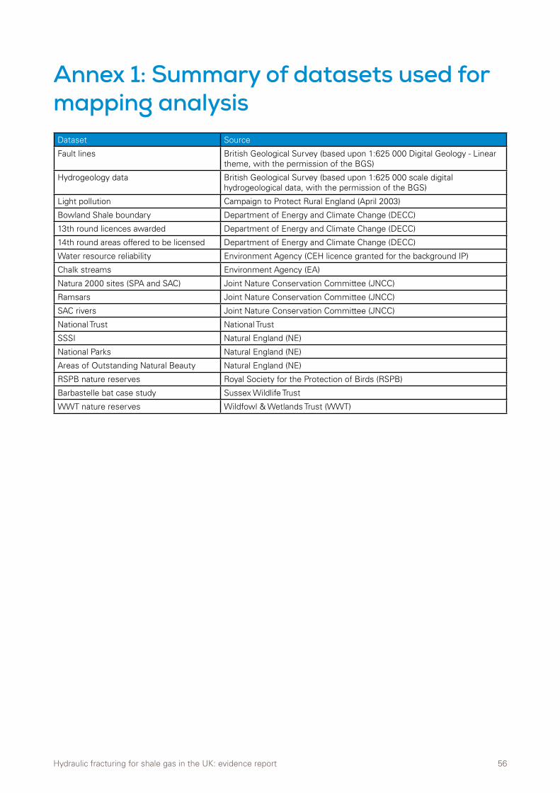
Hydraulic fracturing for shale gas in the UK: evidence report 56
Annex 1: Summary of datasets used for mapping analysis Dataset Source
Fault lines British Geological Survey (based upon 1:625 000 Digital Geology - Linear theme, with the permission of the BGS)
Hydrogeology data British Geological Survey (based upon 1:625 000 scale digital hydrogeological data, with the permission of the BGS)
Light pollution Campaign to Protect Rural England (April 2003)
Bowland Shale boundary Department of Energy and Climate Change (DECC)
13th round licences awarded Department of Energy and Climate Change (DECC)
14th round areas offered to be licensed Department of Energy and Climate Change (DECC)
Water resource reliability Environment Agency (CEH licence granted for the background IP)
Chalk streams Environment Agency (EA)
Natura 2000 sites (SPA and SAC) Joint Nature Conservation Committee (JNCC)
Ramsars Joint Nature Conservation Committee (JNCC)
SAC rivers Joint Nature Conservation Committee (JNCC)
National Trust National Trust
SSSI Natural England (NE)
National Parks Natural England (NE)
Areas of Outstanding Natural Beauty Natural England (NE)
RSPB nature reserves Royal Society for the Protection of Birds (RSPB)
Barbastelle bat case study Sussex Wildlife Trust
WWT nature reserves Wildfowl & Wetlands Trust (WWT)
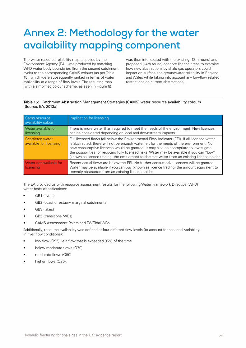
Hydraulic fracturing for shale gas in the UK: evidence report 57
Annex 2: Methodology for the water availability mapping componentThe water resource reliability map, supplied by the Environment Agency (EA), was produced by matching WFD water body boundaries (from the second catchment cycle) to the corresponding CAMS colours (as per Table 15), which were subsequently ranked in terms of water availability at a range of flow levels. The resulting map (with a simplified colour scheme, as seen in Figure 8)
was then intersected with the existing (13th round) and proposed (14th round) onshore licence areas to examine how new abstractions by shale gas operators could impact on surface and groundwater reliability in England and Wales while taking into account any low-flow related restrictions on current abstractions.
Cams resource availability colour
Implication for licensing
Water available for licensing
There is more water than required to meet the needs of the environment. New licences can be considered depending on local and downstream impacts.
Restricted water available for licensing
Full licensed flows fall below the Environmental Flow Indicator (EFI). If all licensed water is abstracted, there will not be enough water left for the needs of the environment. No new consumptive licences would be granted. It may also be appropriate to investigate the possibilities for reducing fully licensed risks. Water may be available if you can “buy” (known as licence trading) the entitlement to abstract water from an existing licence holder.
Water not available for licensing
Recent actual flows are below the EFI. No further consumptive licences will be granted. Water may be available if you can buy (known as licence trading) the amount equivalent to recently abstracted from an existing licence holder.
The EA provided us with resource assessment results for the following Water Framework Directive (WFD) water body classifications:
• GB1 (rivers)
• GB2 (coast or estuary marginal catchments)
• GB3 (lakes)
• GB5 (transitional WBs)
• CAMS Assessment Points and FW Tidal WBs.
Additionally, resource availability was defined at four different flow levels (to account for seasonal variability in river flow conditions):
• low flow (Q95), ie a flow that is exceeded 95% of the time
• below moderate flows (Q70)
• moderate flows (Q50)
• higher flows (Q30).
Table 15: Catchment Abstraction Management Strategies (CAMS) water resource availability colours (Source: EA, 2013a)

Hydraulic fracturing for shale gas in the UK: evidence report 58
Annex 3: Sensitivity mapping for bird disturbance impactsAlthough we concluded that there was insufficient information available to construct a map of bird sensitivity to HVHF activities resulting from shale gas development, before this conclusion was reached efforts were made to try to develop a methodology for mapping bird disturbance.
A natural starting point for identifying species, which could be sensitive to the impacts of HVHF in the UK, is the list of rare and vulnerable species identified under Annex 1 of the European Wild Birds Directive. Many of these have Special Protection Areas (SPAs) which have been identified as areas of international importance for their breeding, feeding, wintering or migration routes. We intersected a map of SPAs in the UK with a map of the 14th round shale gas consultation areas, and identified all species for which SPAs have been designated that fall within the license zones. This resulted in a list of 99 species in total (Table 17).
It was assumed that any sensitivity map would include all SPAs as highly sensitive areas, and that for species where a high proportion of their population was contained within SPAs, the SPA map could provide an adequate surrogate for a species distribution map. However, many
species have only a relatively low proportion of their population contained within SPAs, or spend a significant amount of time in non-designated areas. An internal RSPB workshop was held to identify species with a significant presence outside SPAs that might be particularly sensitive to the disturbance impacts of HVHF. This resulted in the selection of 28 species from the original 99 (Table 16). Two further species, the black grouse and turtle dove, were also identified as being potentially sensitive to disturbance from HVHF and having a significant presence outside SPAs, but within the 14th round consultation zones. This list is based upon expert opinion, and is by no means a comprehensive list of species which may be adversely affected by HVHF activities. Broadly speaking, species belonged to one or more of the following categories:
• Lowland wet grassland breeders (mostly waders)
• Species known to forage outside SPA boundaries
• Species with rare and localised breeding, not well covered by SPAs
• Species with wintering areas outside SPAs.
Common name Scientific name Common name Scientific name Common name Scientific name
Barnacle goose Branta leucopsis [Svalbard/Denmark/UK]
Eurasian oystercatcher
Haematopus ostralegus
Pink-footed goose Anser brachyrhynchus
Black-tailed godwit Limosa limosa islandica
European golden plover
Pluvialis apricaria [North-western Europe - breeding]
Ring ouzel Turdus torquatus
Black-tailed godwit Limosa limosa limosa
European nightjar Caprimulgus europaeus
Ringed plover Charadrius hiaticula
Common pochard Aythya ferina Great bittern Botaurus stellaris Stone-curlew Burhinus oedicnemus
Common redshank Tringa totanus Greater white-fronted goose
Anser albifrons albifrons
Taiga bean goose Anser fabalis fabalis
Common shelduck Tadorna tadorna Hen harrier Circus cyaneus Tundra swan Cygnus columbianus bewickii
Common snipe Gallinago gallinago Lesser black-backed gull
Larus fuscus Whooper swan Cygnus cygnus
Dark-bellied brent goose
Branta bernicla bernicla
Merlin Falco columbarius Woodlark Lullula arborea
Eurasian curlew Numenius arquata Northern lapwing Vanellus vanellus
Eurasian marsh harrier
Circus aeruginosus Peregrine falcon Falco peregrinus
Table 16: Species potentially sensitive to disturbance from HVHF with a significant presence outside SPAs.
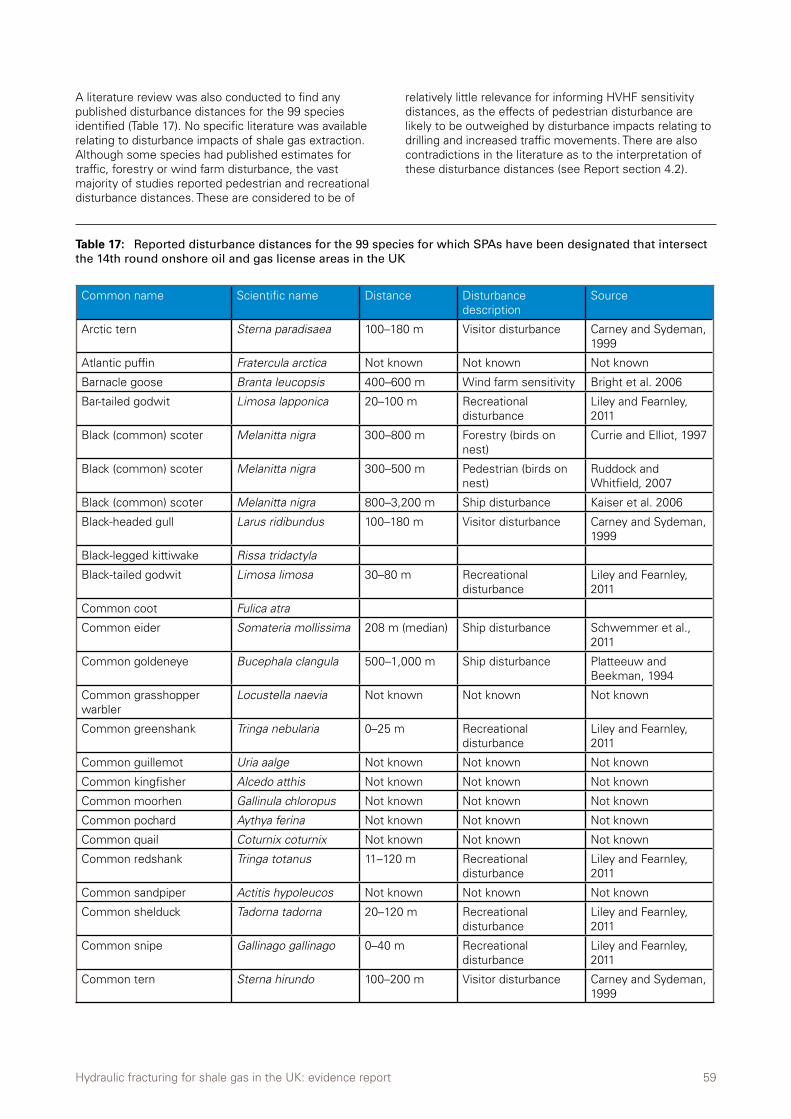
Hydraulic fracturing for shale gas in the UK: evidence report 59
A literature review was also conducted to find any published disturbance distances for the 99 species identified (Table 17). No specific literature was available relating to disturbance impacts of shale gas extraction. Although some species had published estimates for traffic, forestry or wind farm disturbance, the vast majority of studies reported pedestrian and recreational disturbance distances. These are considered to be of
relatively little relevance for informing HVHF sensitivity distances, as the effects of pedestrian disturbance are likely to be outweighed by disturbance impacts relating to drilling and increased traffic movements. There are also contradictions in the literature as to the interpretation of these disturbance distances (see Report section 4.2).
Table 17: Reported disturbance distances for the 99 species for which SPAs have been designated that intersect the 14th round onshore oil and gas license areas in the UK
Common name Scientific name Distance Disturbance description
Source
Arctic tern Sterna paradisaea 100–180 m Visitor disturbance Carney and Sydeman, 1999
Atlantic puffin Fratercula arctica Not known Not known Not known
Barnacle goose Branta leucopsis 400–600 m Wind farm sensitivity Bright et al. 2006
Bar-tailed godwit Limosa lapponica 20–100 m Recreational disturbance
Liley and Fearnley, 2011
Black (common) scoter Melanitta nigra 300–800 m Forestry (birds on nest)
Currie and Elliot, 1997
Black (common) scoter Melanitta nigra 300–500 m Pedestrian (birds on nest)
Ruddock and Whitfield, 2007
Black (common) scoter Melanitta nigra 800–3,200 m Ship disturbance Kaiser et al. 2006
Black-headed gull Larus ridibundus 100–180 m Visitor disturbance Carney and Sydeman, 1999
Black-legged kittiwake Rissa tridactyla
Black-tailed godwit Limosa limosa 30–80 m Recreational disturbance
Liley and Fearnley, 2011
Common coot Fulica atra
Common eider Somateria mollissima 208 m (median) Ship disturbance Schwemmer et al., 2011
Common goldeneye Bucephala clangula 500–1,000 m Ship disturbance Platteeuw and Beekman, 1994
Common grasshopper warbler
Locustella naevia Not known Not known Not known
Common greenshank Tringa nebularia 0–25 m Recreational disturbance
Liley and Fearnley, 2011
Common guillemot Uria aalge Not known Not known Not known
Common kingfisher Alcedo atthis Not known Not known Not known
Common moorhen Gallinula chloropus Not known Not known Not known
Common pochard Aythya ferina Not known Not known Not known
Common quail Coturnix coturnix Not known Not known Not known
Common redshank Tringa totanus 11–120 m Recreational disturbance
Liley and Fearnley, 2011
Common sandpiper Actitis hypoleucos Not known Not known Not known
Common shelduck Tadorna tadorna 20–120 m Recreational disturbance
Liley and Fearnley, 2011
Common snipe Gallinago gallinago 0–40 m Recreational disturbance
Liley and Fearnley, 2011
Common tern Sterna hirundo 100–200 m Visitor disturbance Carney and Sydeman, 1999

Hydraulic fracturing for shale gas in the UK: evidence report 60
Common name Scientific name Distance Disturbance description
Source
Dark-bellied brent goose Branta bernicla bernicla
20–158 m Recreational disturbance
Liley and Fearnley, 2011
Dartford warbler Sylvia undata 50–200 m Forestry (birds on nest)
Currie and Elliot, 1997
Dunlin Calidris alpina 10–300 m Recreational disturbance
Liley and Fearnley, 2011
Eurasian curlew Numenius arquata 20–154 m Recreational disturbance
Liley and Fearnley, 2011
Eurasian hobby Falco subbuteo 180–450 m Forestry (birds on nest)
Forestry Commission, 2006
Eurasian marsh harrier Circus aeruginosus 1,000–2,000 m Wind farm sensitivity Bright et al. 2009
Eurasian marsh harrier Circus aeruginosus 300–500 m Pedestrian (birds on nest)
Ruddock and Whitfield, 2007
Eurasian oystercatcher Haematopus ostralegus
20–500 m Recreational disturbance
Liley and Fearnley, 2011
Eurasian reed warbler Acrocephalus scirpaceus
Not known Not known Not known
Eurasian teal Anas crecca 10–100 m Recreational disturbance
Liley and Fearnley, 2011
Eurasian wigeon Anas penelope 20–190 m Recreational disturbance
Liley and Fearnley, 2011
European golden plover Pluvialis apricaria 90 m Recreational disturbance
Liley and Fearnley, 2011
European honey-buzzard Pernis apivorus 150–600 m Forestry (birds on nest)
Forestry Commission, 2006
European nightjar Caprimulgus europaeus
1,000–2,500 m Wind farm sensitivity Bright et al., 2006
European nightjar Caprimulgus europaeus
50–200 m Forestry (birds on nest)
Forestry Commission, 2006
European nightjar Caprimulgus europaeus
100–150 m Pedestrian (birds on nest)
Ruddock and Whitfield, 2007
European shag Phalacrocorax aristotelis
Not known Not known Not known
Gadwall Anas strepera 110–150 m Recreational disturbance
Liley and Fearnley, 2011
Garganey Anas querquedula Not known Not known Not known
Goosander Mergus merganser Not known Not known Not known
Great bittern Botaurus stellaris Not known Not known Not known
Great cormorant Phalacrocorax carbo 50–100 m Visitor disturbance Carney and Sydeman, 1999
Great crested grebe Podiceps cristatus Not known Not known Not known
Greater scaup Aythya marila 400 m Ship disturbance Platteeuw and Beekman, 1994
Greater white-fronted goose
Anser albifrons albifrons
Not known Not known Not known
Greenland white-fronted goose
Anser albifrons flavirostris
Not known Not known Not known
Grey plover Pluvialis squatarola 20–150 m Recreational disturbance
Liley and Fearnley, 2011
Greylag goose Anser anser Not known Not known Not known
Hen harrier Circus cyaneus 2,000 m Wind farm sensitivity Bright et al., 2006
Hen harrier Circus cyaneus 1,000–2,000 m Wind farm sensitivity Bright et al., 2009
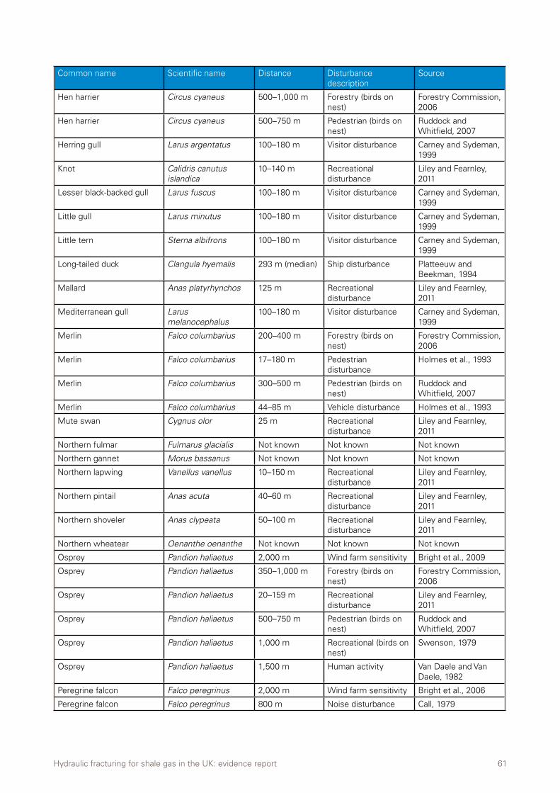
Hydraulic fracturing for shale gas in the UK: evidence report 61
Common name Scientific name Distance Disturbance description
Source
Hen harrier Circus cyaneus 500–1,000 m Forestry (birds on nest)
Forestry Commission, 2006
Hen harrier Circus cyaneus 500–750 m Pedestrian (birds on nest)
Ruddock and Whitfield, 2007
Herring gull Larus argentatus 100–180 m Visitor disturbance Carney and Sydeman, 1999
Knot Calidris canutus islandica
10–140 m Recreational disturbance
Liley and Fearnley, 2011
Lesser black-backed gull Larus fuscus 100–180 m Visitor disturbance Carney and Sydeman, 1999
Little gull Larus minutus 100–180 m Visitor disturbance Carney and Sydeman, 1999
Little tern Sterna albifrons 100–180 m Visitor disturbance Carney and Sydeman, 1999
Long-tailed duck Clangula hyemalis 293 m (median) Ship disturbance Platteeuw and Beekman, 1994
Mallard Anas platyrhynchos 125 m Recreational disturbance
Liley and Fearnley, 2011
Mediterranean gull Larus melanocephalus
100–180 m Visitor disturbance Carney and Sydeman, 1999
Merlin Falco columbarius 200–400 m Forestry (birds on nest)
Forestry Commission, 2006
Merlin Falco columbarius 17–180 m Pedestrian disturbance
Holmes et al., 1993
Merlin Falco columbarius 300–500 m Pedestrian (birds on nest)
Ruddock and Whitfield, 2007
Merlin Falco columbarius 44–85 m Vehicle disturbance Holmes et al., 1993
Mute swan Cygnus olor 25 m Recreational disturbance
Liley and Fearnley, 2011
Northern fulmar Fulmarus glacialis Not known Not known Not known
Northern gannet Morus bassanus Not known Not known Not known
Northern lapwing Vanellus vanellus 10–150 m Recreational disturbance
Liley and Fearnley, 2011
Northern pintail Anas acuta 40–60 m Recreational disturbance
Liley and Fearnley, 2011
Northern shoveler Anas clypeata 50–100 m Recreational disturbance
Liley and Fearnley, 2011
Northern wheatear Oenanthe oenanthe Not known Not known Not known
Osprey Pandion haliaetus 2,000 m Wind farm sensitivity Bright et al., 2009
Osprey Pandion haliaetus 350–1,000 m Forestry (birds on nest)
Forestry Commission, 2006
Osprey Pandion haliaetus 20–159 m Recreational disturbance
Liley and Fearnley, 2011
Osprey Pandion haliaetus 500–750 m Pedestrian (birds on nest)
Ruddock and Whitfield, 2007
Osprey Pandion haliaetus 1,000 m Recreational (birds on nest)
Swenson, 1979
Osprey Pandion haliaetus 1,500 m Human activity Van Daele and Van Daele, 1982
Peregrine falcon Falco peregrinus 2,000 m Wind farm sensitivity Bright et al., 2006
Peregrine falcon Falco peregrinus 800 m Noise disturbance Call, 1979
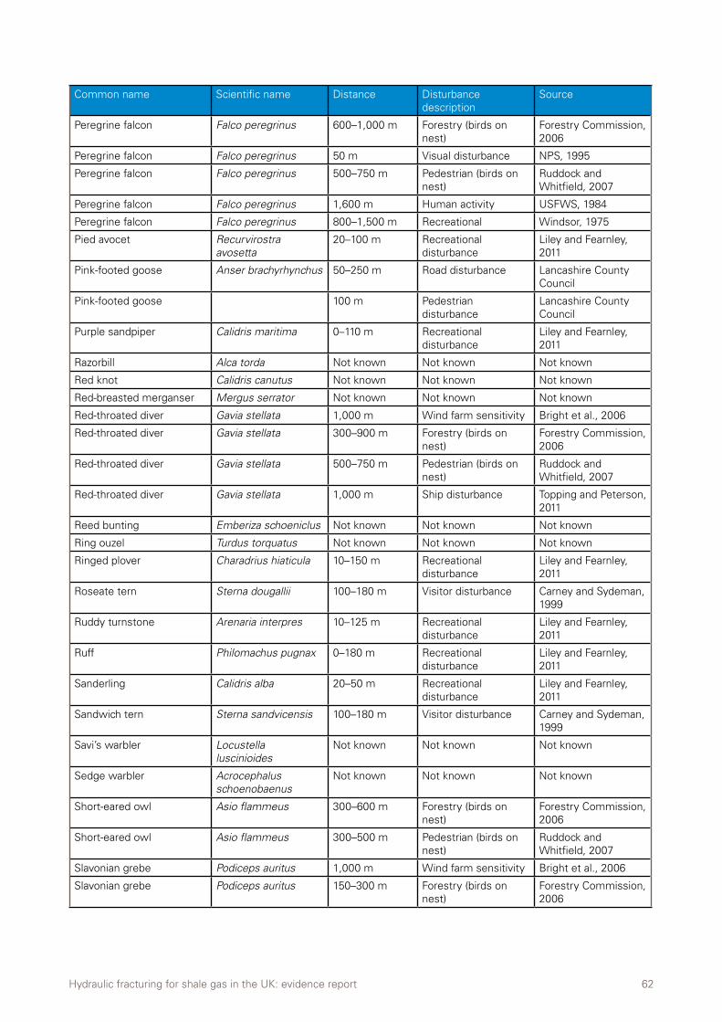
Hydraulic fracturing for shale gas in the UK: evidence report 62
Common name Scientific name Distance Disturbance description
Source
Peregrine falcon Falco peregrinus 600–1,000 m Forestry (birds on nest)
Forestry Commission, 2006
Peregrine falcon Falco peregrinus 50 m Visual disturbance NPS, 1995
Peregrine falcon Falco peregrinus 500–750 m Pedestrian (birds on nest)
Ruddock and Whitfield, 2007
Peregrine falcon Falco peregrinus 1,600 m Human activity USFWS, 1984
Peregrine falcon Falco peregrinus 800–1,500 m Recreational Windsor, 1975
Pied avocet Recurvirostra avosetta
20–100 m Recreational disturbance
Liley and Fearnley, 2011
Pink-footed goose Anser brachyrhynchus 50–250 m Road disturbance Lancashire County Council
Pink-footed goose 100 m Pedestrian disturbance
Lancashire County Council
Purple sandpiper Calidris maritima 0–110 m Recreational disturbance
Liley and Fearnley, 2011
Razorbill Alca torda Not known Not known Not known
Red knot Calidris canutus Not known Not known Not known
Red-breasted merganser Mergus serrator Not known Not known Not known
Red-throated diver Gavia stellata 1,000 m Wind farm sensitivity Bright et al., 2006
Red-throated diver Gavia stellata 300–900 m Forestry (birds on nest)
Forestry Commission, 2006
Red-throated diver Gavia stellata 500–750 m Pedestrian (birds on nest)
Ruddock and Whitfield, 2007
Red-throated diver Gavia stellata 1,000 m Ship disturbance Topping and Peterson, 2011
Reed bunting Emberiza schoeniclus Not known Not known Not known
Ring ouzel Turdus torquatus Not known Not known Not known
Ringed plover Charadrius hiaticula 10–150 m Recreational disturbance
Liley and Fearnley, 2011
Roseate tern Sterna dougallii 100–180 m Visitor disturbance Carney and Sydeman, 1999
Ruddy turnstone Arenaria interpres 10–125 m Recreational disturbance
Liley and Fearnley, 2011
Ruff Philomachus pugnax 0–180 m Recreational disturbance
Liley and Fearnley, 2011
Sanderling Calidris alba 20–50 m Recreational disturbance
Liley and Fearnley, 2011
Sandwich tern Sterna sandvicensis 100–180 m Visitor disturbance Carney and Sydeman, 1999
Savi’s warbler Locustella luscinioides
Not known Not known Not known
Sedge warbler Acrocephalus schoenobaenus
Not known Not known Not known
Short-eared owl Asio flammeus 300–600 m Forestry (birds on nest)
Forestry Commission, 2006
Short-eared owl Asio flammeus 300–500 m Pedestrian (birds on nest)
Ruddock and Whitfield, 2007
Slavonian grebe Podiceps auritus 1,000 m Wind farm sensitivity Bright et al., 2006
Slavonian grebe Podiceps auritus 150–300 m Forestry (birds on nest)
Forestry Commission, 2006
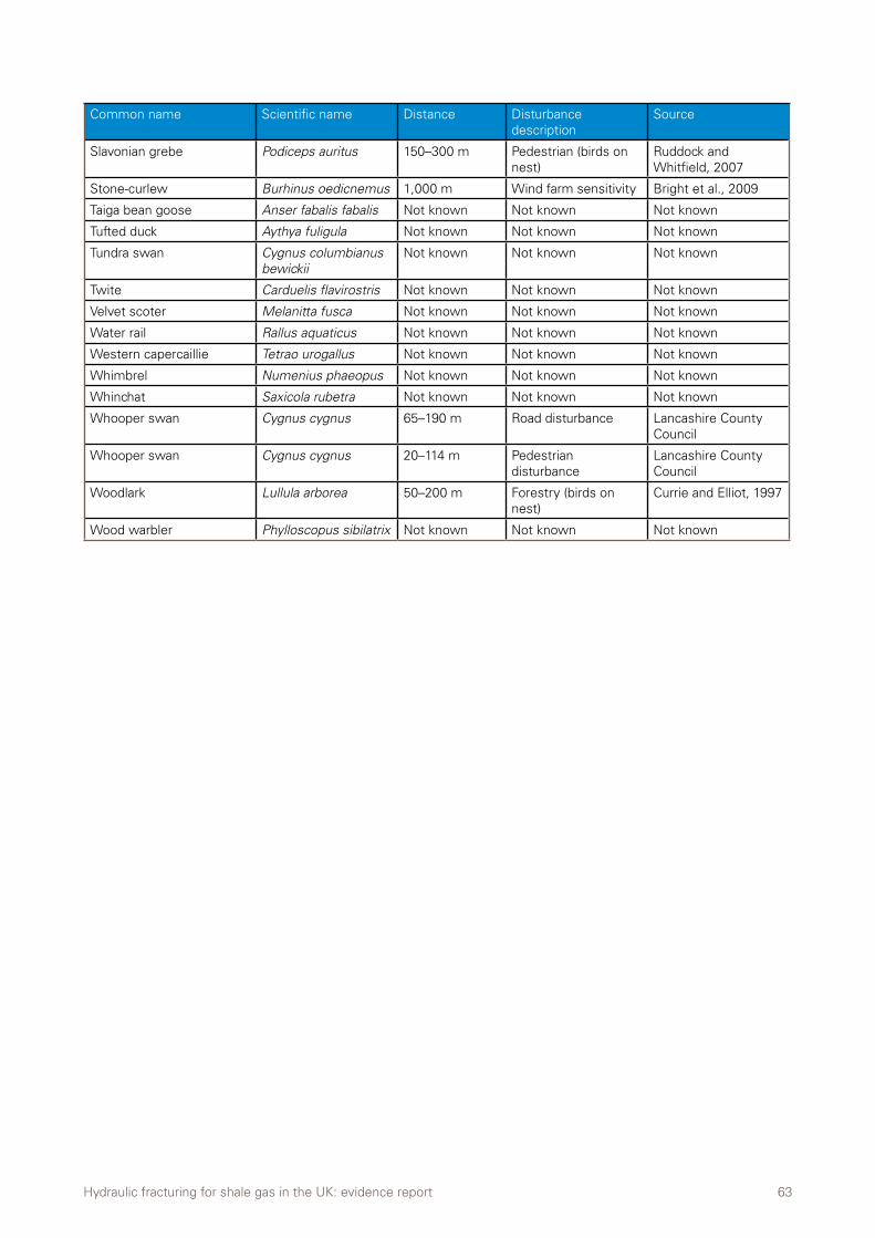
Hydraulic fracturing for shale gas in the UK: evidence report 63
Common name Scientific name Distance Disturbance description
Source
Slavonian grebe Podiceps auritus 150–300 m Pedestrian (birds on nest)
Ruddock and Whitfield, 2007
Stone-curlew Burhinus oedicnemus 1,000 m Wind farm sensitivity Bright et al., 2009
Taiga bean goose Anser fabalis fabalis Not known Not known Not known
Tufted duck Aythya fuligula Not known Not known Not known
Tundra swan Cygnus columbianus bewickii
Not known Not known Not known
Twite Carduelis flavirostris Not known Not known Not known
Velvet scoter Melanitta fusca Not known Not known Not known
Water rail Rallus aquaticus Not known Not known Not known
Western capercaillie Tetrao urogallus Not known Not known Not known
Whimbrel Numenius phaeopus Not known Not known Not known
Whinchat Saxicola rubetra Not known Not known Not known
Whooper swan Cygnus cygnus 65–190 m Road disturbance Lancashire County Council
Whooper swan Cygnus cygnus 20–114 m Pedestrian disturbance
Lancashire County Council
Woodlark Lullula arborea 50–200 m Forestry (birds on nest)
Currie and Elliot, 1997
Wood warbler Phylloscopus sibilatrix Not known Not known Not known
Hydraulic fracturing for shale gas in the UK: evidence report 64
Contact us
Cover: drilling equipment at a shale gas drill site, Southport by Cernan Elias (Alamy).
The Royal Society for the Protection of Birds (RSPB) is a registered charity: England & Wales no. 207076, Scotland no. SC037654 272-1210-13-14
Angling TrustEastwood House, 6 Rainbow Street, Leominster, Herefordshire HR6 8DQTel: 0844 7700616anglingtrust.net
National TrustPO Box 574, Manvers, Rotherham S63 3FHTel: 0844 800 1895nationaltrust.org.uk
The Royal Society for the Protection of Birds (RSPB)The Lodge, Sandy, Bedfordshire SG19 2DL. Tel: 01767 680551rspb.org.uk
Salmon & Trout AssociationFishmongers’ Hall, London Bridge, London EC4R 9EL Tel: 020 7283 5838salmon-trout.org
The Wildlife TrustsThe Kiln, Mather Road, Newark, United Kingdom NG24 1WTTel: 01636 677711wildlifetrusts.org
Wildfowl & Wetlands Trust (WWT)Slimbridge, Gloucestershire GL2 7BTTel: 01453 891900wwt.org.uk


