Lecture 6—Evaporation and Transpiration I like to start talking about the water cycle with evaporation, in large part because I tend to think of the “cycle” as having a flat spot—water gets evaporated, precipitated, and runs off within days to weeks, but upon rearrival in the oceans, it’ll be there a while. So, let’s talk about how moisture gets up into the atmosphere in the first place. There are two basic mechanisms by which moisture gets into the atmosphere; evaporation and transpiration. They’re basically the same thing, in the end. Evaporation is just a phase change in water (from liquid to vapor) induced by the addition of enough energy (remember that water has a high heat of vaporization—it takes 600 calories to vaporize 1 gram of liquid water). What’s actually happening is that the relatively loose bonds between water molecules (remember, because they’re polar, they have a loose hydrogen bond) are broken with the addition of enough energy, allowing individual molecules of water to float free. You probably remember that the two things that drive this process are how much energy is available (and for our purposes, most of this energy is sunlight), and how much water is already in the atmosphere (remember chemistry class? Dalton’s Law dictates how much vapor can actually be held in the atmosphere. Once the atmosphere is saturated with water, you can’t put any more in). Transpiration is the same thing (conversion of liquid water to water vapor), but it’s biologically mediated, and it’s dominated by plants. Plants have developed a very efficient system for pulling water up from the ground based on capillary action. In order to drive the pump, water vapor is ejected from leaf surfaces through small openings called stomata. Stomata can be opened and stopped down, thus allowing the plant to regulate how much water it gives off. They serve a second purpose, too. Ejecting water vapor enables plants to regulate leaf temperature the same way sweat enables us to regulate temperature. Other sources of water vapor (respiration by animals, sublimation of ice directly to water vapor, water vapor expelled by volcanoes) are relatively unimportant (on this planet, in a global scale). The amount of water vapor produced by ice on Mars, for example, is currently a
Transcript
Lecture 6—Evaporation and Transpiration I like to start talking about the water cycle with evaporation, in large part because I tend to think of the “cycle” as having a flat spot—water gets evaporated, precipitated, and runs off within days to weeks, but upon rearrival in the oceans, it’ll be there a while. So, let’s talk about how moisture gets up into the atmosphere in the first place. There are two basic mechanisms by which moisture gets into the atmosphere; evaporation and transpiration. They’re basically the same thing, in the end. Evaporation is just a phase change in water (from liquid to vapor) induced by the addition of enough energy (remember that water has a high heat of vaporization—it takes 600 calories to vaporize 1 gram of liquid water). What’s actually happening is that the relatively loose bonds between water molecules (remember, because they’re polar, they have a loose hydrogen bond) are broken with the addition of enough energy, allowing individual molecules of water to float free. You probably remember that the two things that drive this process are how much energy is available (and for our purposes, most of this energy is sunlight), and how much water is already in the atmosphere (remember chemistry class? Dalton’s Law dictates how much vapor can actually be held in the atmosphere. Once the atmosphere is saturated with water, you can’t put any more in). Transpiration is the same thing (conversion of liquid water to water vapor), but it’s biologically mediated, and it’s dominated by plants. Plants have developed a very efficient system for pulling water up from the ground based on capillary action. In order to drive the pump, water vapor is ejected from leaf surfaces through small openings called stomata. Stomata can be opened and stopped down, thus allowing the plant to regulate how much water it gives off. They serve a second purpose, too. Ejecting water vapor enables plants to regulate leaf temperature the same way sweat enables us to regulate temperature. Other sources of water vapor (respiration by animals, sublimation of ice directly to water vapor, water vapor expelled by volcanoes) are relatively unimportant (on this planet, in a global scale). The amount of water vapor produced by ice on Mars, for example, is currently a
matter of some debate. Equally, the amount of water expelled by Pu’u O’o is locally important. So, most of the time we care about the conversion of liquid water to water vapor in standing bodies of water and the expelling of water vapor by plants. Because we don’t really care which one caused the water to get into the atmosphere, we often combine these two terms to form evapotranspiration or ET. Our interest is not entirely academic. It turns out there are tables and tables of data on how much water crops need, and at what stage in their growth. And, because people have been growing crops for much longer than they’ve been describing the water cycle, it’s little wonder that most of our instrumentation for measuring ET comes from agriculture. Quantifying ET The first, and oldest, method for estimating how much water evaporates from an area is to put out a pan of water, and measure how much water leaves the pan in a day. Yep, that’s it. The crazy part is that this remains the primary method for determining ET. I’m not kidding. The “pan” in this case is generally normalized (so we’re all using the same pan), and it comes with a whole list of rules about where to put the pan, but in the end, it’s a pan of water. In the US, the pan is 4 feet in diameter, and 1 foot deep, and it’s called a Class A Pan. You put a stilling well in the pan so that you’re actually measuring the water level and not waves (even little waves) in the pan, then you measure the water level with a hook gauge, which gets you to water level changes within about 0.01”. Because the pan is out in the open, you also have to worry about rain getting into the pan, and you need a rain gauge, too (more on these later). These are not without problems. First, they’re made of stainless steel, and they sit off the ground so the sides are exposed. This means that a little more evaporation happens in the pan than evaporates from the ground nearby. As a result, most pans have a correction factor (called the pan coefficient) based on their location—you multiply the pan evaporation by the pan coefficient to get the “actual” evaporation. The average pan coefficient in the U.S. is about 0.7. Moreover, keeping animals from drinking the water out of a pan means a rather substantial investment in fencing.
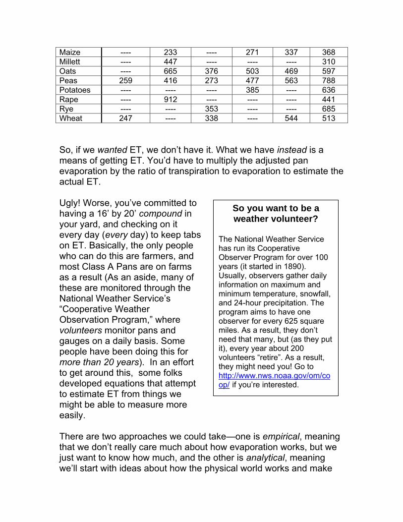
The point is that a pan takes up a lot of room and requires someone to monitor it every day. Next problem. The pan actually measures evaporation, not evapotranspiration. This doesn’t seem like an issue, but it turns out that of the two, transpiration totally dominates the system in vegetated areas. Take a look: Crop Harpenden,
Maize ---- 233 ---- 271 337 368 Millett ---- 447 ---- ---- ---- 310 Oats ---- 665 376 503 469 597 Peas 259 416 273 477 563 788 Potatoes ---- ---- ---- 385 ---- 636 Rape ---- 912 ---- ---- ---- 441 Rye ---- ---- 353 ---- ---- 685 Wheat 247 ---- 338 ---- 544 513 So, if we wanted ET, we don’t have it. What we have instead is a means of getting ET. You’d have to multiply the adjusted pan evaporation by the ratio of transpiration to evaporation to estimate the actual ET. Ugly! Worse, you’ve committed to having a 16’ by 20’ compound in your yard, and checking on it every day (every day) to keep tabs on ET. Basically, the only people who can do this are farmers, and most Class A Pans are on farms as a result (As an aside, many of these are monitored through the National Weather Service’s “Cooperative Weather Observation Program,” where volunteers monitor pans and gauges on a daily basis. Some people have been doing this for more than 20 years). In an effort to get around this, some folks developed equations that attempt to estimate ET from things we might be able to measure more easily. There are two approaches we could take—one is empirical, meaning that we don’t really care much about how evaporation works, but we just want to know how much, and the other is analytical, meaning we’ll start with ideas about how the physical world works and make
So you want to be a weather volunteer?
The National Weather Service has run its Cooperative Observer Program for over 100 years (it started in 1890). Usually, observers gather daily information on maximum and minimum temperature, snowfall, and 24-hour precipitation. The program aims to have one observer for every 625 square miles. As a result, they don’t need that many, but (as they put it), every year about 200 volunteers “retire”. As a result, they might need you! Go to http://www.nws.noaa.gov/om/coop/ if you’re interested.
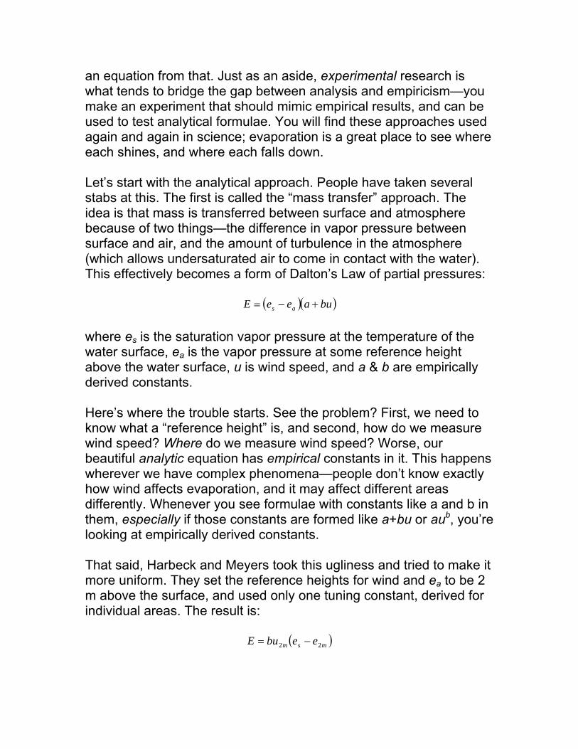
an equation from that. Just as an aside, experimental research is what tends to bridge the gap between analysis and empiricism—you make an experiment that should mimic empirical results, and can be used to test analytical formulae. You will find these approaches used again and again in science; evaporation is a great place to see where each shines, and where each falls down. Let’s start with the analytical approach. People have taken several stabs at this. The first is called the “mass transfer” approach. The idea is that mass is transferred between surface and atmosphere because of two things—the difference in vapor pressure between surface and air, and the amount of turbulence in the atmosphere (which allows undersaturated air to come in contact with the water). This effectively becomes a form of Dalton’s Law of partial pressures:
( )( )buaeeE as +−= where es is the saturation vapor pressure at the temperature of the water surface, ea is the vapor pressure at some reference height above the water surface, u is wind speed, and a & b are empirically derived constants. Here’s where the trouble starts. See the problem? First, we need to know what a “reference height” is, and second, how do we measure wind speed? Where do we measure wind speed? Worse, our beautiful analytic equation has empirical constants in it. This happens wherever we have complex phenomena—people don’t know exactly how wind affects evaporation, and it may affect different areas differently. Whenever you see formulae with constants like a and b in them, especially if those constants are formed like a+bu or aub, you’re looking at empirically derived constants. That said, Harbeck and Meyers took this ugliness and tried to make it more uniform. They set the reference heights for wind and ea to be 2 m above the surface, and used only one tuning constant, derived for individual areas. The result is:
( )msm eebuE 22 −=
This brings up another point about analysis. In general, formulae derived from the same basic assumptions (in this case mass transfer) tend to look alike. Notice that we still have a vapor pressure difference in here, and that we’re still multiplying by wind speed. This is important, because all analytical equations are built on assumptions, and most of the time people won’t tell you what those assumptions were. Being able to figure out what kind of equation something is, and therefore what its internal assumptions are, is a valuable skill. Some people find mass transfer less than satisfying. It still has an empirical constant in it, and therefore suggests we don’t really understand what’s going on. Another approach would be to make, effectively, an energy budget for the atmosphere and the water surface, and see what happens. Let’s see, we’ve got solar radiation being absorbed by the water, call it QN. We’re losing that energy by both conductive and convective heat transfer to the atmosphere, that’s Qh. It takes a certain amount of energy to evaporate water, so we lose that, too. That’s Qe. We’ve got to have a storage term, too. That’d be Qθ here, and effectively tracks the change in temperature of the water. Last, we need to handle energy that’s advected into the area by groundwater and surface water—that’s Qv. Ok, if Qv is positive for energy coming in, then:
hevN QQQQQ ++=+ θ This points out another feature of truly analytical equations—they may be exact, but they’re useless because we can’t measure any of these things. Let’s make it easier—we want evaporation, so let’s rearrange for that. Taking Le to be the latent heat of vaporization (which handles Qe), and R to be the ratio of heat lost by conduction to that lost by evaporation (handling Qh), we’ve got:
( )RLQQQ
Ee
vN
+−+
=1ρ
θ
Which is at least slightly nicer to use. Still, what’s R? R can be determined from:
as
as
as
as
eeTTP
eeTT
R−−
=⎟⎠⎞
⎜⎝⎛⎟⎟⎠
⎞⎜⎜⎝
⎛−−
= γ1000
66.0
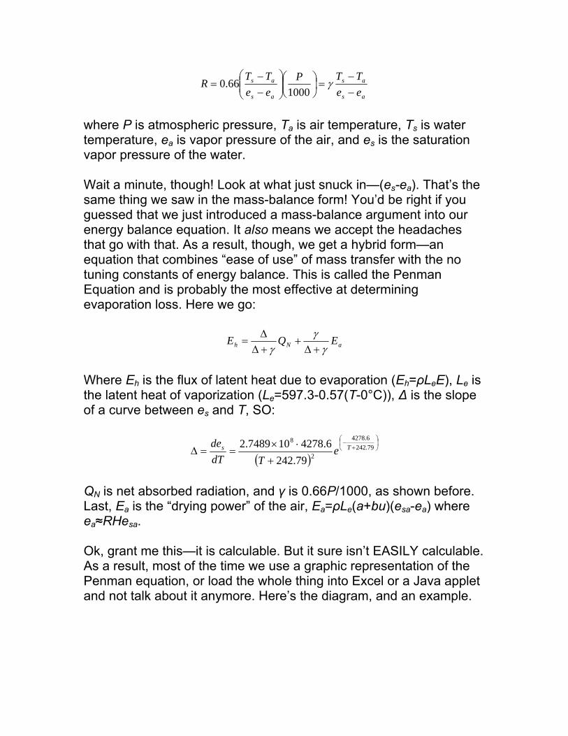
where P is atmospheric pressure, Ta is air temperature, Ts is water temperature, ea is vapor pressure of the air, and es is the saturation vapor pressure of the water. Wait a minute, though! Look at what just snuck in—(es-ea). That’s the same thing we saw in the mass-balance form! You’d be right if you guessed that we just introduced a mass-balance argument into our energy balance equation. It also means we accept the headaches that go with that. As a result, though, we get a hybrid form—an equation that combines “ease of use” of mass transfer with the no tuning constants of energy balance. This is called the Penman Equation and is probably the most effective at determining evaporation loss. Here we go:
aNh EQEγ
γγ +∆
++∆∆
=
Where Eh is the flux of latent heat due to evaporation (Eh=ρLeE), Le is the latent heat of vaporization (Le=597.3-0.57(T-0°C)), ∆ is the slope of a curve between es and T, SO:
( )⎟⎠⎞
⎜⎝⎛
+−
+⋅×
==∆ 79.2426.4278
2
8
79.2426.4278107489.2 Ts e
TdTde
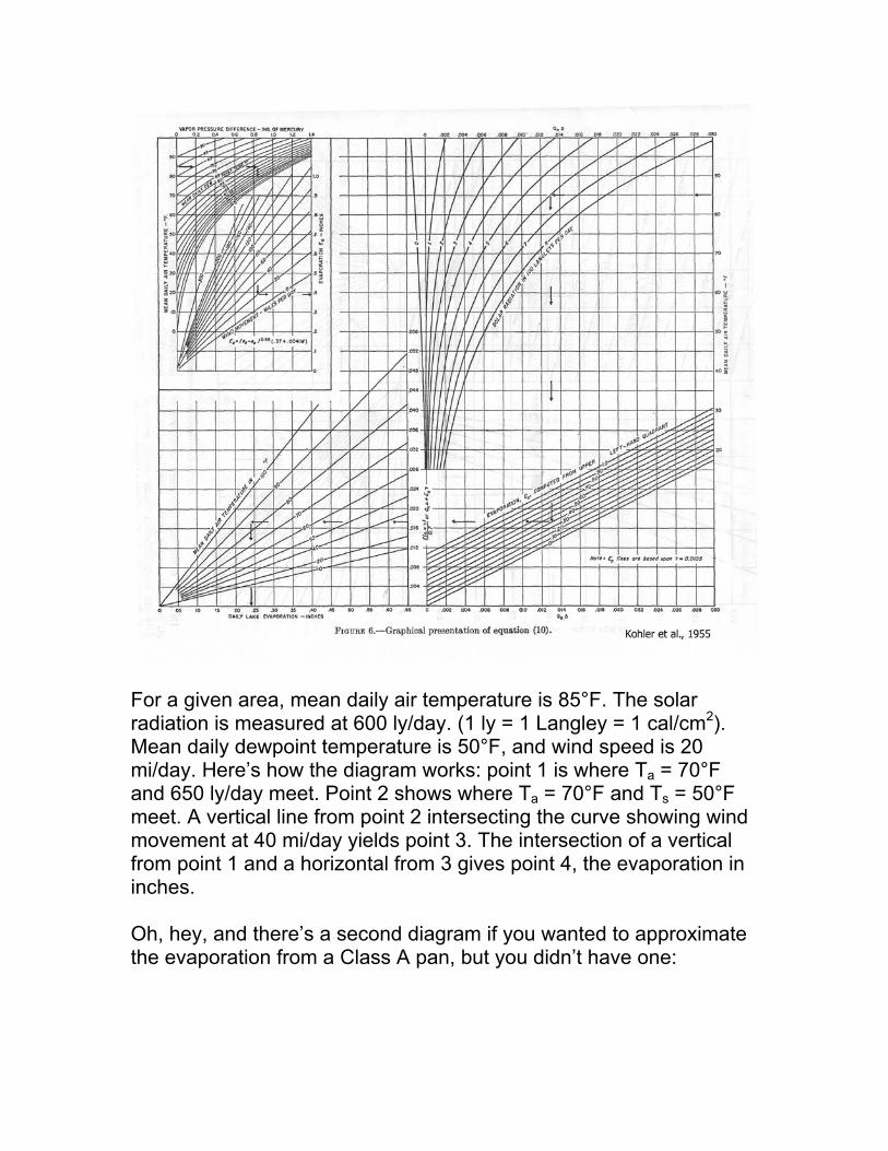
QN is net absorbed radiation, and γ is 0.66P/1000, as shown before. Last, Ea is the “drying power” of the air, Ea=ρLe(a+bu)(esa-ea) where ea≈RHesa. Ok, grant me this—it is calculable. But it sure isn’t EASILY calculable. As a result, most of the time we use a graphic representation of the Penman equation, or load the whole thing into Excel or a Java applet and not talk about it anymore. Here’s the diagram, and an example.
For a given area, mean daily air temperature is 85°F. The solar radiation is measured at 600 ly/day. (1 ly = 1 Langley = 1 cal/cm2). Mean daily dewpoint temperature is 50°F, and wind speed is 20 mi/day. Here’s how the diagram works: point 1 is where Ta = 70°F and 650 ly/day meet. Point 2 shows where Ta = 70°F and Ts = 50°F meet. A vertical line from point 2 intersecting the curve showing wind movement at 40 mi/day yields point 3. The intersection of a vertical from point 1 and a horizontal from 3 gives point 4, the evaporation in inches. Oh, hey, and there’s a second diagram if you wanted to approximate the evaporation from a Class A pan, but you didn’t have one:
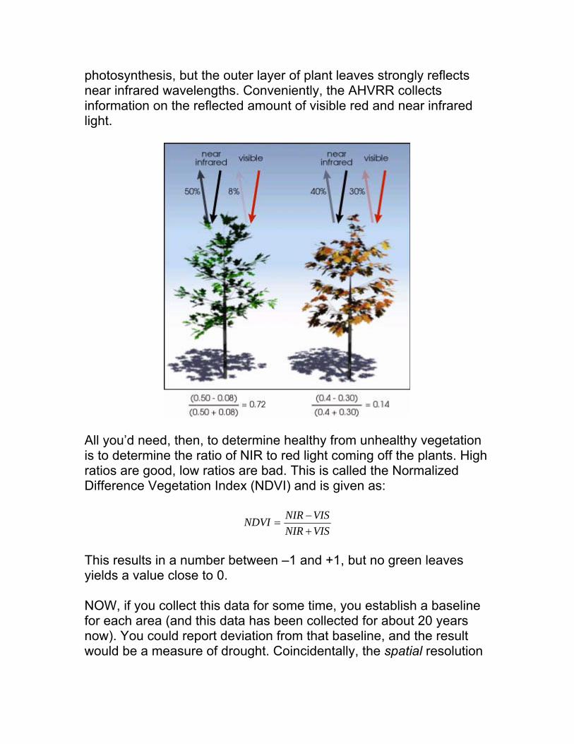
The Penman Equation enables us to get rid of the evaporation pans. This is good. It has a long history, and is well benchmarked, which is also good. The problem is that we still need a bunch of data that requires special instruments to determine (like wind speed and solar insolation). Worse, it still doesn’t measure transpiration, which we already know dominates vegetated areas. Suffice it to say it works fine over the ocean (which is great for some things, like hurricane generation). Recently, there’s been an attempt to get around the whole mess and measure transpiration directly. These methods hinge on the Advanced Very High Resolution Radiometer (AHVRR) carried on several NOAA satellites. The AHVRR collects information on how much light of different wavelengths is reflected from earth’s surface. Chlorophyll, in particular, absorbs visible light for use in
photosynthesis, but the outer layer of plant leaves strongly reflects near infrared wavelengths. Conveniently, the AHVRR collects information on the reflected amount of visible red and near infrared light.
All you’d need, then, to determine healthy from unhealthy vegetation is to determine the ratio of NIR to red light coming off the plants. High ratios are good, low ratios are bad. This is called the Normalized Difference Vegetation Index (NDVI) and is given as:
VISNIRVISNIRNDVI
+−
=
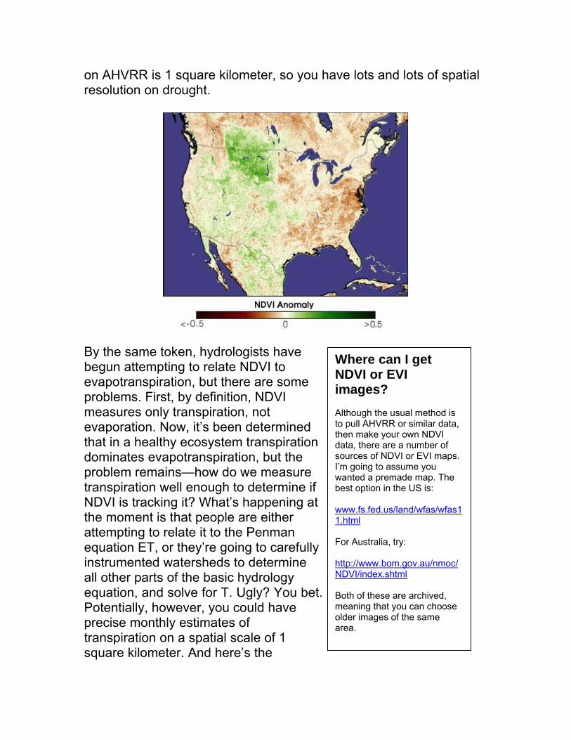
This results in a number between –1 and +1, but no green leaves yields a value close to 0. NOW, if you collect this data for some time, you establish a baseline for each area (and this data has been collected for about 20 years now). You could report deviation from that baseline, and the result would be a measure of drought. Coincidentally, the spatial resolution
on AHVRR is 1 square kilometer, so you have lots and lots of spatial resolution on drought.
By the same token, hydrologists have begun attempting to relate NDVI to evapotranspiration, but there are some problems. First, by definition, NDVI measures only transpiration, not evaporation. Now, it’s been determined that in a healthy ecosystem transpiration dominates evapotranspiration, but the problem remains—how do we measure transpiration well enough to determine if NDVI is tracking it? What’s happening at the moment is that people are either attempting to relate it to the Penman equation ET, or they’re going to carefully instrumented watersheds to determine all other parts of the basic hydrology equation, and solve for T. Ugly? You bet. Potentially, however, you could have precise monthly estimates of transpiration on a spatial scale of 1 square kilometer. And here’s the
Where can I get NDVI or EVI images? Although the usual method is to pull AHVRR or similar data, then make your own NDVI data, there are a number of sources of NDVI or EVI maps. I’m going to assume you wanted a premade map. The best option in the US is: www.fs.fed.us/land/wfas/wfas11.html For Australia, try: http://www.bom.gov.au/nmoc/NDVI/index.shtml Both of these are archived, meaning that you can choose older images of the same area.
teaser—NOAA’s new generation of satellites is up there now, with better color resolution, and 16 times the spatial resolution. The current satellite gives a pixel size of 250 meters on a side. This has given rise to a new vegetation index, the Enhanced Vegetation Index (EVI). EVI is formulated in much the same way as NDVI, but allows for increased resolution near saturation (NDVI values near 1).