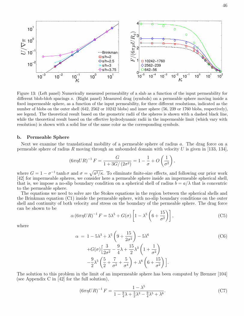
Hydrodynamics of Suspensions of Passive and Active Rigid Particles:A Rigid Multiblob Approach

Florencio Balboa Usabiaga,1 Bakytzhan Kallemov,1, 2 Blaise Delmotte,1

Amneet Pal Singh Bhalla,3 Boyce E. Griffith,3, 4 and Aleksandar Donev1, ∗

1Courant Institute of Mathematical Sciences,New York University, New York, NY 10012

2Energy Geosciences Division, Lawrence Berkeley National Laboratory, Berkeley, CA, 947203Department of Mathematics, University of North Carolina, Chapel Hill, NC 27599

4Department of Biomedical Engineering, University of North Carolina, Chapel Hill, NC 27599

We develop a rigid multiblob method for numerically solving the mobility problemfor suspensions of passive and active rigid particles of complex shape in Stokes flow inunconfined, partially confined, and fully confined geometries. As in a number of existingmethods, we discretize rigid bodies using a collection of minimally-resolved sphericalblobs constrained to move as a rigid body, to arrive at a potentially large linear system ofequations for the unknown Lagrange multipliers and rigid-body motions. Here we developa block-diagonal preconditioner for this linear system and show that a standard Krylovsolver converges in a modest number of iterations that is essentially independent of thenumber of particles. Key to the efficiency of the method is a technique for fast computa-tion of the product of the blob-blob mobility matrix and a vector. For unbounded suspen-sions, we rely on existing analytical expressions for the Rotne-Prager-Yamakawa tensorcombined with a fast multipole method (FMM) to obtain linear scaling in the number ofparticles. For suspensions sedimented against a single no-slip boundary, we use a directsummation on a Graphical Processing Unit (GPU), which gives quadratic asymptoticscaling with the number of particles. For fully confined domains, such as periodic suspen-sions or suspensions confined in slit and square channels, we extend a recently-developedrigid-body immersed boundary method [“An immersed boundary method for rigid bod-ies”, B. Kallemov, A. Pal Singh Bhalla, B. E. Griffith, and A. Donev, Communications inApplied Mathematics and Computational Science, 11-1, 79-141, 2016] to suspensions offreely-moving passive or active rigid particles at zero Reynolds number. We demonstratethat the iterative solver for the coupled fluid and rigid body equations converges in abounded number of iterations regardless of the system size. In our approach, each iter-ation only requires a few cycles of a geometric multigrid solver for the Poisson equation,and an application of the block-diagonal preconditioner, leading to linear scaling withthe number of particles. We optimize a number of parameters in the iterative solvers andapply our method to a variety of benchmark problems to carefully assess the accuracy ofthe rigid multiblob approach as a function of the resolution. We also model the dynamicsof colloidal particles studied in recent experiments, such as passive boomerangs in a slitchannel, as well as a pair of non-Brownian active nanorods sedimented against a wall.

I. Introduction

The study of the hydrodynamics of colloidal suspensions of passive particles is an old yet still activesubject in soft condensed matter physics and chemical engineering. In recent years there has been a growinginterest in suspensions of active colloids [1], which exhibit rich collective behaviors quite distinct fromthose of passive suspensions. There is a growing number of computational methods for modeling activesuspensions [2–9], which are typically built upon well-developed techniques for passive suspensions in steadyStokes flow, i.e., at zero Reynolds number. Since active particles typically have metallic subcomponents,they are often significantly denser than the solvent and sediment toward the bottom wall, making itnecessary to address confinement and implement non-periodic boundary conditions in any method aimed

∗Electronic address: donev@courant.nyu.edu

2

at simulating experimentally-relevant configurations. Furthermore, since collective motions seen in activesuspensions involve large numbers of particles, and since hydrodynamic interactions among particlesdecay slowly like the inverse of the distance, it is crucial to develop methods that can capture long-rangedhydrodynamic effects, yet still scale to tens or hundreds of thousands of particles.

For suspensions of passive particles the methods of Brownian [10, 11] and Stokesian dynamics [12, 13] havedominated in chemical engineering, and related techniques have been used in biochemical engineering [14–18].These methods simulate the overdamped (diffusive) dynamics of the particles by using Green’s functions forsteady Stokes flow to capture the effect of the fluid. While this sort of implicit solvent approach works very wellin many situations, it has several notable technical difficulties: achieving near linear scaling for many-particlesystems is technically challenging, handling non-trivial boundary conditions (bounded systems) is complicatedand has to be done on a case-by-case basis [13, 19–28], generalizations to non-spherical (and in particularcomplex) particle shapes is difficult, and including thermal fluctuations is non-trivial due to the need toobtain stochastic increments with the desired covariance. In this work we develop relatively low-accuracy butflexible and simple rigid multiblob methods that address these difficulties. Our approach builds heavily on anumber of existing techniques, combining elements from several distinct but related methods. We extensivelytest the proposed methods and study their accuracy and performance on a number of test problems.

The continuum formulation of the Stokes equations with suitable boundary conditions on the surfacesof a collection of rigid particles is well-known and summarized in more detail in Appendix A. Due tothe linearity of the Stokes equations, there is an affine mapping from the applied forces f and torquesτ and any specified apparent slip velocity due to active boundary layers u, to the resulting particle motiongiven by the linear velocities u and the angular velocities ω. Specifically,[

uω

]=N

[fτ

]− N u, (1)

where N is the mobility matrix, and N is an active mobility linear operator. The mobility problem consistsof computing the rigid-body motion given the applied forces and torques and apparent slip. The inverseof this problem is the resistance problem, which computes the forces and torques on the body given aspecified motion of the body and active slip. Solving the mobility problem is a key component of anynumerical method for modeling the deterministic or fluctuating (Brownian) dynamics of the particles.

In this paper we develop a mobility solver for suspensions of rigid particles immersed in viscous fluid,specifically, we develop novel preconditioners for iterative solvers for the unknown motions of the rigidbodies, given the applied external forces and torques as well as active apparent slip on the surface of theparticles. As we discuss in more detail in the body of the paper, our formulation can readily solve theresistance problem; however, our iterative solvers will prove to be more scalable for mobility computations(which are of primary interest) than for resistance computations. Key to the success of our iterativesolvers is the idea that instead of eliminating variables using exact Schur complements and solving areduced system iteratively, as done in the majority of existing methods [5, 29, 30], one should insteaditeratively solve an extended system that includes all of the variables. This has the key advantage that thematrix-vector product becomes an efficient direct calculation, and the Schur complement can be computedonly approximately and used to construct an effective preconditioner.

Like many other authors, we construct rigid bodies of essentially arbitrary shape as a collection of rigidly-connected collection of “blobs” or“beads” forming a composite object [29] that we will refer to as a rigid multi-blob. The hydrodynamic interactions between blobs are represented using a Rotne-Prager tensor generalized tothe desired domain geometry (boundary conditions) [31], specifically, we use the the Rotne-Prager-Yamakawa(RPY) tensor [32] for an unbounded domain, and the Rotne-Prager-Blake (RPB) tensor [13] for a half-spacedomain. In Section II we describe how to obtain the hydrodynamic coupling between a large collection of rigidmultiblobs by solving a large linear system for Lagrange multipliers enforcing the rigidity. A key contributionof our work is to develop an indefinite saddle-point preconditioner for iterative solution of the resulting linearsystem. This preconditioner is based on a block-diagonal approximation of the blob-blob mobility matrix, inwhich all hydrodynamic interactions among distinct bodies (more precisely, among blobs on distinct bodies)are neglected. The only system-specific component is the implementation of a fast matrix-vector multiplica-tion routine, which in turn requires a scalable method for multiplying the RPY mobility matrix by a vector.

For simple geometries such as an unbounded domain or particles sedimented next to a no-slip boundary,simple analytical formulas for the RPY tensor are well-known [13, 31], and can be used to construct an

3

efficient matrix-vector multiplication routine, for example, using fast multipole methods (FMMs) [33, 34],or even direct summation on a GPU. We numerically study the performance and accuracy of the rigidmultiblob methods for suspensions in an unbounded domain in Section IV, and study particles sedimentednear a no-slip boundary in Section V. We find that resolving spherical particles with twelve blobs placedon the vertices of an icosahedron [35] is notably more accurate than the FTS (force-torque-stresslet plusdegenerate quadrupole) truncation typically employed in Stokesian dynamics simulations, provided thatthe effective hydrodynamic radius of the rigid multiblob is adjusted to account for the finite size of theblobs. We also find that a small number of iterations of a Krylov method are required to solve the requiredlinear system, and importantly, the number of iterations is constant independent of the the number ofrigid bodies, making it possible to develop a linear or near-linear scaling algorithm. For resistance problems,however, we observe a number of iterations growing at least as fast as the linear dimensions of the system.This is consistent with similar studies of iterative solvers for Stokesian dynamics by Ichiki [36].

For confined systems, however, even in the simplest case of a periodic system, the Green’s function for Stokesflow and the associated RPY tensor is difficult to obtain in closed form, and when it is possible to write an ana-lytical result, the resulting formulas are typically based on infinite series that are expensive to evaluate. For pe-riodic systems this is commonly addressed by using Ewald summation [37] based on the fast Fourier transform(FFT) [29]; the present state-of-the-art for Stokes flow is the spectral Ewald method [25], which has recentlybeen used for Stokesian dynamics simulations of periodic suspensions [38]. A key deficiency of most existingmethods is that they rely critically on having triply periodic domains and the use of the FFT. Generalizingthese methods to non-periodic domains while keeping their linear scaling requires a large development effortand typically a new implementation for every different geometry [26, 28]. Furthermore, in a number of applica-tions involving active particles [39, 40], there is a surface slip (e.g., electrohydrodynamic or osmophoretic flow)induced on the bottom boundary due to the gradients created by the particles, and this slip drives or at leaststrongly affects the motion of the particles. Accounting for this slip requires solving an additional equationsuch as a Poisson or Laplace equation for the electric potential or concentration of chemical fuel with nontriv-ial boundary conditions on the particle and wall surfaces. The solution of this additional equation providesthe slip boundary condition for the Stokes equations, which must be solved to find the resulting fluid flow andactive particle motion. Such nontrivial multi-physics coupling is quite hard to accomplish in existing methods.

To address these difficulties, in Section III we develop a method for general cuboidal confined domains whichdoes not require analytical Green’s functions. This relies on an immersed boundary (IB) method for obtainingan approximation to the RPY tensor in confined geometries, as recently developed by some of us [41]. Thistechnique has been combined with the concept of multiblob representation of rigid bodies in a follow-up work[35], but in this work stiff elastic springs were used to enforce the rigidity. By contrast, we ensure the rigidityof the multiblobs via Lagrange multipliers which are solved concurrently with solving for the fluid pressureand velocity. Our key novel contribution is an effective preconditioner for the rigidly-constrained Stokesproblem in periodic and non-periodic domains, obtained by combining our recently-developed preconditionerfor a rigid-body IB method [42] with a block-diagonal preconditioner for the mobility subproblem.

In the IB method developed in Section III and studied numerically in Section VI, analytical Green’s func-tions are replaced by an “on the fly” computation carried out by a standard finite-volume fluid solver. ThisStokes solver can readily handle nontrivial boundary conditions, for example, slip along the walls [39, 40] caneasily be accounted for. Furthermore, suspensions at small but nonzero Reynolds numbers can be handledwith little extra work [42, 43]. Additionally, we avoid uncontrolled approximations relying on truncations ofmultipole expansions to a fixed order [2, 12, 43, 44], and we can seamlessly handle arbitrary body shapes anddeformation kinematics. Lastly, and importantly, in the spirit of fluctuating hydrodynamics [41, 45, 46], it isstraightforward to generate the stochastic increments required to simulate the Brownian motion of small rigidparticles suspended in a fluid by including a fluctuating stress in the fluid equations, as we will discuss in moredetail in future work; here we focus on the deterministic mobility and resistance problems. At the same time,our method also has some disadvantages compared to methods such as boundary integral or boundary elementmethods. Notably, it requires filling the domain with a dense uniform fluid grid, which is expensive at low den-sities. It is also a low-order method that cannot compute solutions as accurately as spectral boundary integralformulations. We do believe, nevertheless, that the method developed here offers a good compromise betweenaccuracy, efficiency, scalabilty, flexibility and extensibility, compared to other more specialized formulations.

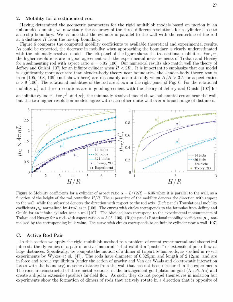
We apply our methods to a number of test problems for which analytical solutions are known, but also studya few nontrivial problems that have not been properly addressed in the literature. In Section V B we study themobility of a cylinder of finite aspect ratio that is parallel to a no-slip boundary and compare to experimental

4

measurements and asymptotic theory based on a slender-body approximation. In Section V C we study theformation of a stable rotating pair of active “extensor” or “pusher” nanorods next to a no-slip boundary, andconfirm the direction of rotation observed in recent experiments [47]. In Section VI D we compute the effectivediffusion coefficient of a boomerang-shaped colloid in a slit channel, and compare to recent experimentalmeasurements [48, 49]. In Section VI F we study the mean and variance of the sedimentation velocity in abinary suspension of spheres of size ratio two, and compare to recent Stokesian dynamics simulations [38, 50].

II. Rigid Multiblob Models of Colloidal Suspensions

In this section we develop the rigid multiblob model of colloidal particles at zero Reynolds number.The kind of models we use here are not new, but we present the method in detail instead of relying onprevious presentations, the most relevant of which are those of Swan et al. [5, 29]. This is in part topresent the formulation in our notation, and in part to explain the differences with other closely-relatedmethods. Our key novel contribution in this section is the preconditioned iterative solver described inSection II B; the performance and scaling of our mobility solver is studied numerically for unboundeddomains in Section IV D, and for particles confined near a single wall in Section V D.

The modeling of suspensions of rigid spheres at small Reynolds numbers is a well-developed field with along history. A powerful class of methods are related to Brownian Dynamics with Hydrodynamic Interactions(BDHI) [10, 11, 51, 52] and Stokesian Dynamics (SD) [12–14, 20, 38, 53] (note that these terms are useddifferently in different communities). The difference between these two (as we define them here) is that BDHIuses what we call a minimally-resolved model [41] in which each colloid (for colloidal suspensions) or polymerbead (for polymeric suspensions) is only resolved at the monopole level, more precisely, at the Rotne-Pragerlevel [29]. By contrast, in SD the next level in a multipole expansion is taken into account and torques andstresslets are also accounted for. It has been shown recently that yet one more order needs to be kept in themultipole expansion to model suspensions of active spheres [2, 8], and a suitable Galerkin truncation of themultipole hierarchy has been developed for active spheres in unbounded domains [8], as well as for activespheres confined near a no-slip boundary [9]. It is also possible to account for higher-order multipoles [8, 54–57], leading to more complicated (and computationally expensive) but also more accurate models. It has alsobeen shown that multipole expansions converge very poorly for nearly touching spheres due to the divergenceof the lubrication forces, and in most methods for dense colloidal suspensions of hard spheres pairwise lubrica-tion corrections are added in a somewhat ad hoc manner; we will refer to this approach as SD with lubrication.

Given the well-developed tools for modeling sphere suspensions, it is natural to leverage them whenmodeling suspensions of particles of more complex shapes. Here we describe a technique capable of, inprinciple, modeling passive rigid particles of arbitrary shape. The method can also be used to model, withoutany extra effort, active particles with active slip layers, i.e., particles which are phoretic (e.g., osmo-phoretic,electro-phoretic, chemo-phoretic, etc.) due to an apparent slip at their surface. For the purposes ofhydrodynamic calculations, we discretize rigid bodies by constructing them out of multiple rigidly-connectedspherical “blobs” or beads of hydrodynamic radius a. These blobs can be thought of as hydrodynamicallyminimally-resolved spheres forming a rigid conglomerate that approximates the hydrodynamics of theactual rigid object being studied. We prefer the word “blob” over “sphere” or “point” or “monopole” becauseblobs are not spheres as they do not have a well-defined surface like spheres do, they have a finite sizeassociated with them (the hydrodynamic blob radius a) unlike points, and they account for a degeneratequadrupole associated to the Faxen corrections in addition to a force monopole. The word “bead” is alsoappropriate, but we prefer to reserve that for polymer models (bead-spring or bead-link models).

Examples of “multiblob” [35] models of two types of colloidal particles are illustrated in Fig. 1. In theleftmost panel, we show a minimally-resolved model of a rigid rod, with dimensions similar to active metallic“nanorods” used in recent experiments [47, 58]. In this minimally-resolved model the blobs, shown asspheres with radius equal to a, are placed in a row along the axes of the cylinder. Such minimally-resolvedmodels are particularly suited for cylinders of large but finite aspect ratio; for very thin rods such as actinfilaments boundary integral methods based on slender-body theory [59] will be more effective. In themore resolved model illustrated in the second panel from the left, a hexagon of blobs is placed aroundthe circumference of the cylinder to better resolve it. A yet more resolved model with a dodecagon ofblobs around the cylinder circumference is shown in the third panel from the left. In the rightmost panelof Fig. 1 we show a blob model of a colloidal boomerang with a square cross-section, as manufacturedusing lithography and studied in [48]. Similar “bead” or “raspberry” models appear in a number of studiesof hydrodynamics of particle suspensions [5, 6, 14–17, 35, 60–66].

In many studies, stiff elastic springs between the blobs are used to keep the structure rigid; in some models

5

Figure 1: Rigid multiblob models of colloidal particles manufactured in recent experimental work. (Left threepanels) A cylinder of aspect ratio of about six, similar to the active nanorods studied experimentally in [47, 58],for three different resolutions; from left to right: minimally-resolved model with 14 blobs, marginally-resolvedmodel with 86 blobs, and well-resolved model with 324 blobs. (Rightmost panel) A 120-blob model of a boomerangwith square cross-section, as studied experimentally in [48].

the fluid or particle inertia is included also. Here, we keep the structures strictly rigid and refer to the resultingstructures as rigid multiblob models. Such rigid multiblob models have been used in a number of prior studies[5, 14–17, 60, 64, 67], but we refer to [5] for a detailed exposition. Our primary focus in this section will be todevelop algorithmic techniques that allow suspensions of tens or even hundreds of thousands of rigid multiblobparticles to be simulated efficiently. This is in many ways primarily an exercise in numerical linear algebra,but one that is necessary to make the rigid multiblob approach useful for simulating moderately densesuspensions. A second goal, which will be realized in the results sections of this paper, will be to carefullyassess the accuracy of rigid multiblob models as a function of their resolution (number of blobs per body).

A. Hydrodynamics of rigid multiblobs

We now summarize the main equations used to solve the mobility and resistance problems for a collectionof rigid multiblobs immersed in a viscous fluid. We first discuss the hydrodynamic interaction betweenblobs, and then discuss the hydrodynamic interactions between rigid bodies.

In the notation used below, we will use the Latin indices i, j, k, l for individual blobs, and reserve Latinindices p, q, r, s for bodies. We will denote with Bp the set of blobs comprising body p. We will consider asuspension of N rigid bodies with a chosen reference tracking point on body p having position qp, and the orien-tation of body p relative to a reference configuration represented by the quaternion θp [68]. The linear velocityof (the chosen tracking point on) body p will be denoted with up, and its angular velocity will be denoted withωp. The total force applied on body p is f p, and the total torque is τ p. The composite configuration vector

of position and orientation of body p will be denoted with Qp =qp, θp

, the composite vector of linear and

angular velocity will be denoted with U p = up, ωp, and the composite vector of forces and torques withF p =

f p, τ p

. The position of blob i ∈ Bp will be denoted with ri, and its velocity will be denoted with ri.

When not subscripted, vectors will refer to the composite vector formed by all bodies or all blobs on all bodies.For example, U will denote the linear and angular velocities of all bodies, and r will denote the positions of allof the blobs. We will use a superscript to denote portions of composite vectors for all blobs belonging to onebody, for example, r(p) = ri | i ∈ Bp will denote the vector of positions of all blobs belonging to body p.

The fact that the multiblob p is rigid is expressed by the “no-slip” kinematic condition,

ri = up + ωp ×(ri − qp

), ∀i ∈ Bp. (2)

This no-slip condition can be written for all bodies succinctly as

r = KU , (3)

where K (Q) is a simple geometric matrix [29]. We will denote the apparent velocity of the fluid at point riwith wi ≈ v (ri). For a passive blob, i.e., a blob that represents a passive part of the rigid particle, the no-slipboundary condition requires that wi = ri. However, for active blobs an additional apparent slip of the fluid

6

relative to the surface of the body can be imposed, resulting in a nonzero slip ui = wi−ri. This kind of activepropulsion is termed “implicit swimming gait” by Swan and Brady [13]. An “explicit swimming gait” [13] canbe taken into account without any modifications to the formulation or algorithm by simply replacing (2) with

wi = ri + ui = up + ωp × (ri − qp) + ui. (4)

That is, the only difference between “slip” and “deformation” is whether the blobs move relative to the rigidbody frame dragging the fluid along, or stay fixed in the body frame while the fluid passes by them. Onecan of course even combine the two and have the blobs move relative to the rigid body while also pushingflow, for example, this can be used to model an active filament where there is slip along the filament but thefilament itself is moving. In the end, the only thing that matters to the formulation is the velocity difference

ui ≈ v (ri)−(up + ωp ×

(ri − qp

)). (5)

In Appendix C we explain how to model permeable (porous) bodies by making the apparent slipproportional to the fluid-blob force λ.

The fundamental problem tackled in this paper is the solution of the mobility problem, that is, the compu-tation of the motion of the bodies given the applied forces and torques on the bodies and the slip velocity. Be-cause of the linearity of the Stokes equations and the boundary conditions, there exists an affine linear mapping

U =NF − Mu,

where the body mobility matrix N (Q) depends on the configuration and is the central object of the

computation. The active mobility matrix M is a discretization of the active mobility operator N , andgives the active motion of force- and torque-free particles. Note that M is related to, but different from,the propulsion matrix introduced in [8]. The propulsion matrix is essentially a finite-dimensional projection

of the operator N that only depends on the choice of basis functions used to express the surface slipvelocity u, and does not depend on the specific discretization of the body or quadrature rules, as does M.

In the remainder of this section we develop a method for computing U given F and u, i.e., a methodfor computing the combined action of N and M, for large collections of non-overlapping rigid particles.We will also briefly discuss the resistance problem, in which we are given the motion of the bodies asa specified kinematics, and seek the resulting drag forces and torques, which have the form

F =RU + Ru,

where the body resistance matrix R =N−1 and R =N−1M is the active resistance matrix.

1. Blob mobility matrix

The blob-blob translational mobility matrixM describes the hydrodynamic interactions between theNb blobs, accounting for the influence of the boundaries. Specifically, if the blobs are free to move (i.e.,not constrained rigidly) with the fluid under the action of set of translational forces λi, the translationalvelocities of the blobs will be

w = r + u =Mλ. (6)

The mobility matrix M is a block matrix of dimension (dNb) × (dNb), where d is the dimensionality.The d× d blockMij computes the velocity of blob i given the force on blob j, neglecting the presenceof the other blobs in a pairwise approximation.

To construct a suitable M, we can think of blobs as spheres of hydrodynamic radius a. For twowell-separated spheres i and j of radius a we have the far-field approximation [13, 31, 52]

Mij ≈ η−1

(I +

a2

6∇2

r′

)(I +

a2

6∇2

r′′

)G(r′, r′′)

∣∣r′=rj ,

r′′=ri,(7)

where η is the fluid viscosity and G is the Green’s function for the steady Stokes problem with unit viscosity,with the appropriate boundary conditions such as no-slip on the boundaries of the domain. The differential

7

operator I + (a2/6)∇2 is called the Faxen operator [52]. Note that the form of (7) guarantees that themobility matrix is symmetric positive semidefinite (SPD) by construction since G is an SPD kernel.

For a three dimensional unbounded domain with fluid at rest at infinity, the Green’s function is isotropicand given by the Oseen tensor,

G(r′, r′′) ≡ O(r = r′ − r′′) =1

8πr

(I +

r ⊗ rr2

). (8)

Using this expression in (7) yields the far-field component of the Rotne-Prager-Yamakawa (RPY) tensor[32], commonly used in BDHI. A correction needs to be introduced when particles are close to each otherto ensure an SPD mobility matrix [32], which can be derived by using an integral form of the RPY tensorvalid even for overlapping particles [31], to give

Mij =1

6πηa

C1(rij)I + C2(rij)

rij⊗rij

r2ij, rij > 2a

C3(rij)I + C4(rij)rij⊗rij

r2ij, rij ≤ 2a

(9)

where rij = ri − rj, and

C1(r) =3a

4r+

a3

2r3, C2(r) =

3a

4r− 3a3

2r3,

C3(r) = 1− 9r

32a, C4(r) =

3r

32a.

The diagonal blocks of the mobility matrix, i.e., the self-mobility can be obtained by setting rij = 0 to

obtainMii = (6πηa)−1 I, which matches the Stokes solution for the drag on a translating sphere; thisis an important continuity property of the RPY tensor [69]. We will use the RPY tensor (9) for simulationsof rigid-particle suspensions in unbounded domains in Section IV.

In principle, it is possible to generalize the RPY tensor to any flow geometry, i.e., to any boundary conditions(and imposed external flow) [31], including periodic domains [37, 70], as well as confined domains [13, 20].However, we are not aware of any tractable analytical expressions for the complete RPY tensor (includingnear-field corrections) even for the simplest confined geometry of particles near a single no-slip boundary. Inthe presence of a single no-slip wall, an analytic approximation toMij is given by Swan and Brady [13] (andre-derived later in [71]) as a generalization of the Rotne-Prager (RP) tensor [32] to account for the no-slipboundary using Blake’s image construction [72]. As shown in Ref. [31], the corrections to the Rotne-Pragertensor (7) for particles that overlap each other but not the wall are independent of the boundary conditions,and are thus given by the standard RPY expressions (9) for unbounded domains. Therefore, in Section V wecomputeM by adding to the RPY tensor (9) wall corrections corresponding to the translation-translationpart of the Rotne-Prager-Blake mobility given by Eqs. (B1) and (C2) in [13], ignoring the higher order torqueand stresslet terms in the spirit of the minimally-resolved blob model. The expressions derived by Swan andBrady [13] assume that neither particle overlaps the wall and the resulting expressions are not guaranteedto lead to an SPDM if one or more blobs overlap the wall, as we discuss in more detail in the Conclusions.

For more complicated geometries, such as a slit or a square (duct) channel, analytical computations ofthe Green’s function become quite complicated and tedious, and numerical computations typically requirepre-tabulations [20, 52, 73]. In Section VI we explain how a grid-based finite volume Stokes solver can be usedto obtain the action of the Green’s function and thus compute the action of the mobility matrix for confineddomains, for essentially arbitrary combinations of periodic, free-slip, no-slip, or stress boundary conditions.

2. Body mobility matrix

After discretizing the rigid bodies as rigid multiblobs, we can write down a system of equations thatconstrain the blobs to move rigidly in a straightforward manner. Letting λ be a vector of forces (Lagrangemultipliers) that acts on each blob to enforce the rigidity of the body, we have the following linear system

8

for λ, u, and ω for all bodies p,∑j

Mijλj =up + ωp ×(ri − qp

)+ ui, ∀i ∈ Bp, (10)∑

i∈Bp

λi =f p,∑i∈Bp

(ri − qp)× λi =τ p.

The first equation is the no-slip condition obtained by combining (6) and (2). The second and third equationsare the force and torque balance conditions for body p. Note that the physical interpretation of λ is that of atotal force on the portion of the surface of the body associated with a given blob. If one wants to think of (10)as a regularized discretization of the first-kind integral equation (A5) and obtain a pointwise value of the trac-tion force density, one should divide λj by the surface area ∆Aj associated with blob j, which plays the roleof a quadrature weight [67]; we will discuss more sophisticated quadrature rules [74, 75] in the Conclusions.

We can write the mobility problem (10) in compact matrix notation as a saddle-point linear systemof equations for the rigidity forces λ and unknown motion U ,[

M −K−KT 0

] [λU

]=

[u−F

]. (11)

Forming the Schur complement by eliminating λ we get (see also Eq. (1) in [5] or Eq. (32) in [29])

U =NF −(NKTM−1

)u =NF − Mu,

where the body mobility matrix N is

N =(KTM−1K

)−1, (12)

and is evidently SPD since M is. Although written in this form using the inverse of M, unlike in anumber of prior works [14–16, 60, 64], we obtain U by solving (11) directly using an iterative solver, aswe explain in more detail in Section II B. We note that one can compute a fluid velocity field v (r) fromλ using a procedure we describe in Appendix B.

The resistance problem, on the other hand, consists of solving for λ in

Mλ = KU + u, (13)

and then computing F = KTλ, giving

F =(KTM−1K

)U +

(KTM−1

)u =RU + Ru.

At first glance, it appears that solving the resistance system (13) is easier than solving the saddle-pointproblem (11); however, as we explain in more detail in Section IV D, the mobility problem is significantlyeasier to solve using iterative methods than the resistance problem, consistent with similar observationsin the context of Stokesian Dynamics [36]. Observe that the saddle-point formulation (11) applies morebroadly to mixed mobility/resistance problems, where some of the rigid body degrees of freedom areconstrained but some are free [76]. An example is a suspension of spheres being rotated by a magneticfield at a specified angular velocity but free to move translationally, or a suspension of colloids fixed inspace by strong laser tweezers but otherwise free to rotate, or even a hinged body that can only move ina partially-constrained manner. In cases such as these we simply redefine U to contain the free kinematicdegrees of freedom and modify the definition of the kinematic matrix K. Much of what we say belowcontinues to apply, but with the caveat that the expected speed of convergence of iterative methods isexpected to depend on the nature of the imposed constraints, as we discuss in Section IV D.

9

Note that the formula (12) is somewhat formal, and in practice all inverses should be replaced bypseudo-inverses. For instance, in the limit when infinitely many blobs cover the surface of a body, themobility matrixM is not invertible since making λ perpendicular to the surface will not yield any flowbecause it will try to compress the (fictitious) incompressible fluid inside the body. Note that this nontrivialnull space of the mobility poses no problem when using an iterative method to solve (11) because the righthand side is in the proper range due to the imposition of the volume-preservation constraint (A6). It is alsopossible that the matrix KTM−1K is not invertible. A typical example for this is the minimally-resolvedcylinder shown in the left-most panel of Fig. 1. Because all of the forces λ are applied exactly on thesemi-axes of the cylinder, they cannot exert a torque around the symmetry axes of the rod. Again, thereis no problem with iterative solvers for (11) if the applied force is in the appropriate range (e.g., one shouldnot apply a torque around the semi-axes of a minimally-resolved cylinder).

B. Iterative Mobility Solver

For a small number of blobs, the equation (11) can be solved by direct inversion ofM, as done in mostprior works. For large systems, which is the focus of our work, iterative methods are required. A standardapproach used in the literature is to eliminate one of the variables λ orU . Eliminating λ leads to the equation(

KTM−1K)U = F −KTM−1u, (14)

which requires the action ofM−1, which must itself be obtained inside a nested iterative solver, increasingboth the complexity and the cost of the method. Swan and Wang [29] have recently used the ConjugateGradient method to solve (14), preconditioning using the block-diagonal matrix P = (6πηa)

(KTK

).

An alternative is to write an equivalent system to (11), for an arbitrary constant c 6= 0,[M −K

−KT (I + cM) c(KTK

) ] [ λU

]=

[u

−(F + cKT u

) ] , (15)

from which we can easily eliminate U to obtain an equation for λ only, in the form[M(I −K(KTK)−1KT

)− c−1K(KTK)−1KT

]λ = rhs, (16)

where we omit the full expression for the right hand side for brevity. The system (16) can now be solvedusing (preconditioned) conjugate gradients, and only requires the inverse of the simpler matrix KTK.Note that, although not presented in this way, this is the essence of the approach that is followed andrecommended by Swan et al. [5] (see Appendix [5] and note that c is denoted by λ in that paper); they

recommend computing the action of(KTK

)−1by an iterative method preconditioned by an incomplete

Cholesky factorization. A similar approach is followed in boundary integral formulations (which areusually formulated using a double layer density), where a continuum operator related to K(KTK)−1KT

is computed and then discretized using a quadrature rule [27, 77].In contrast to the approaches taken by Swan et al. [5, 29], we have found that numerically the best

approach to solving for the unknown rigid-body motions of the particles is to solve the extended saddle-pointproblem (11) for both U and λ directly, using a preconditioned iterative Krylov method. In fact, as wewill demonstrate in the results section of this paper, such an approach has computational complexitythat is essentially linear in the number of blobs because the number of iterations required to solve (11)is quite modest when an appropriate preconditioner, described below, is used. This approach does not

require computing (the action of)(KTK

)−1and leads to a very simple implementation.

1. Matrix-Vector Product

A Krylov solver for (11) requires two components:

1. An efficient algorithm for performing the matrix-vector product, which in our case amounts to a fastmethod to multiply the dense but low-rank mobility matrixM by a vector of blob forces λ.

2. A suitable preconditioner, which is an approximate solver for (11).

10

How to efficiently computeMλ depends very much on the boundary conditions and thus the form ofthe Green’s function used to constructM. For unbounded domains, in this work we use the Fast MultipoleMethod (FMM) developed specifically for the RPY tensor in [33]; alternative kernel-independent FMMscould also be used, and have also been generalized to periodic domains [78]. The FMM method hasan essentially linear computational cost of O (Nb logNb) for a single matrix-vector multiplication. Inthe simulations presented here we use a fixed and rather tight relative tolerance for the FMM ∼ 10−9

throughout the iterative solution process. Krylov methods, however, allow one to lower the accuracyof the matrix-vector product as the residual is reduced [79]; this has recently been used to lower the costof FMM-based boundary integral methods [80]. We will explore such optimizations in future work.

For rigid particles sedimented near a single no-slip wall, we have implemented a Graphics ProcessingUnit (GPU) based direct summation matrix-vector product based on the Rotne-Prager-Blake tensor derivedby Swan and Brady [13]. This has, asymptotically, a quadratic computational cost of O (N2

b ); however,the computation is trivially parallel so the multiplication is remarkably fast even for one million blobsbecause of the very large number of threads available on modern GPUs. Gimbutas et al. have recentlydeveloped an FMM method for the Blake tensor by using a simple image construction (image Stokesletplus a harmonic scalar correction) and applying an infinite-space FMM method to the extended system ofsingularities [34]. However, this construction has not yet been generalized to the Rotne-Prager-Blake tensor,and, furthermore, the FMM will not be more efficient than the direct product on GPUs in practice unlessa large number of blobs is considered. For fully confined domains, we will adopt an extended saddle-pointformulation that will be described in Section VI.

2. Preconditioner

In this work we demonstrate that a very efficient yet simple preconditioner for (11) is obtained byneglecting hydrodynamic interactions between different bodies, that is, setting the elements of Mcorresponding to pairs of blobs on distinct bodies to zero in the preconditioner. This amounts to making a

block-diagonal approximation of the mobility M defined by only keeping the diagonal blocks correspondingto a single body interacting only with the boundaries of the domain,

M(pq)

= δpqM(pp). (17)

We will demonstrate here that the indefinite block-diagonal preconditioner,

P =

[M −K−KT 0

], (18)

is a very effective preconditioner for solving (11).Applying the preconditioner (18) amounts to solving the linear system[

M −K−KT 0

] [λU

]=

[u−F

], (19)

which is quite easy to do since the approximate body mobility matrix (Schur complement),

N =(KTM

−1K)−1

,

is itself a block-diagonal matrix where each block on the diagonal refers to a single body neglecting allhydrodynamic interactions with other bodies,

N pq = δpq

((K(p)

)T (M(pp)

)−1

K(p)

)−1

.

Computing N pq requires a dense matrix inversion (e.g., Cholesky factorization) of the much smaller

mobility matrix M(pp), whose size is(dN

(p)b

)×(dN

(p)b

), where N

(p)b is the number of blobs on body

11

p. In the case of an infinite domain, the factorization ofM(pp) can be precomputed once at the beginningof a dynamic simulation and reused during the simulation due to the rotational and translational invarianceof the RPY tensor; one only needs to apply rotation matrices to the right-hand side and the result toconvert between the original reference configuration of the body and the current configuration. Furthermore,particles of the same shape and size discretized with the same number of blobs as body p can share a single

factorization ofM(pp) and N pp. In cases whereM(pp) depends in a nontrivial way on the position of the

body, as for (partially) confined domains, one needs to factorizeM(pp) for all bodies p at every time step;this factorization can still be reused during the iterative solve in each application of the preconditioner.

Because our preconditioner is indefinite, one cannot use the preconditioned Conjugate Gradient (PCG)Krylov method to solve (11) without modification. One of the most robust iterative methods, which weuse in this work, is the Generalized Minimum Residual Method (GMRES). The key advantage of GMRESis that it is guaranteed to reduce the residual from iteration to iteration. Its main downside is that itrequires storing a large number of intermediate vectors (i.e., the history of the iterates). GMRES alsocan stall, although this can be corrected to some extent by restarts. An alternative to GMRES is the(stabilized) Bi-Conjugate Gradient (BiCG(Stab)) method, which works for non-symmetric matrices aswell. In our implementation we have relied on the PETSc library [81] for iterative solvers; this librarymakes it very easy to experiment with different iterative solvers.

III. Rigid Multiblobs in Confined Domains

The rigid multiblob method described in Section II requires a technique for multiplying the blob-blobmobility matrix with a vector. Therefore, this approach, like all other Green’s function based methods [8, 13,20, 23–28, 52, 54–57], is very geometry-specific and does not generalize easily to more complicated boundaryconditions. To handle geometries for which there is no simple analytical expression for the Green’s function,such as slit or square channels, pre-tabulation of the Green’s function is necessary, and ensuring a positivesemi-definite mobility matrix is in general difficult. Another difficulty with Green’s function based methodsis that including a “background” flow is only simple when this flow can be computed easily analytically,such as simple shear flows. But for more complicated geometries, such as Poiseuille flow through a squarechannel, computing the base flow is itself not trivial or requires evaluating expensive infinite-series solutions.

An alternative approach is to use a traditional Stokes solver to solve the fluid equations numerically [11].This requires filling the domain with a grid, which can increase the number of degrees of freedom considerablyover just discretizing the surface of the immersed bodies. However, the number of fluid degrees of freedomcan be held approximately constant as more bodies are included, so that the methods typically scale very wellwith the number of particles and are well-suited to dense particle suspensions. Previous work [41, 46, 82] hasshown how to use an immersed boundary (IB) method [83] to obtain the action of the Green’s function incomplex geometries. In this approach, spherical particles are minimally resolved using only a single blob perparticle. In subsequent work this approach was extended to multiblob models [35], but the rigidity constraintwas imposed only approximately using stiff springs, leading to numerical stiffness. A class of related minimally-resolved methods based on the Force Coupling Method (FCM) [30, 44, 45, 84] can include also torques andstresslets, as well as particle activity [4], but a number of these methods have relied strongly on periodicboundaries since they use the Fast Fourier Transform (FFT) to solve the (fluctuating) Stokes equations.

In recent work [42], some of us have developed an IB method for rigid bodies. This method appliesto a broad range of Reynolds numbers. In the case of zero Reynolds number it becomes equivalent tothe rigid multiblob method presented in Section II, but with a blob-blob mobility that is computed bythe fluid solver. In Ref. [42] only rigid bodies with specified motion (kinematics) were considered; here weextend the method to handle freely-moving rigid bodies in Stokes flow. We will present here the key ideasand focus on the new components necessary to solve for the unknown motion of the particles; we refer thereader interested in more technical details to Refs. [41, 42]. The key novel contribution of our work is thepreconditioner described in Section III C; the performance and scalability of our preconditioned iterativesolvers is studied numerically in Section VI E. To begin, we present a semi-continuum formulation where therelation to Section II is most obvious, and then we discuss the fully discrete formulation used in the actualimplementation. In Appendix C we demonstrate how to handle permeable bodies using a small modificationof the formulation. Numerical results obtained using the method described here are given in Section VI.

12

A. Semi-Continuum Formulation

We consider here a semi-discrete model in which the rigid body has already been discretized using blobsbut a continuum description is used for the fluid, that is, we consider a rigid multiblob model immersedin a continuum Stokesian fluid. In the IB literature blobs are referred to as markers, and are often thoughtof as “points” or “discrete delta functions”. We use the term “blob,” however, to connect to Section IIand to emphasize that the blobs have a finite physical and hydrodynamic extent.

In the IB method [83] (and also the force coupling method [84]), the shape of the blob and its effectiveinteraction with the fluid is captured through a smooth kernel function δa (r) that integrates to unityand whose support is localized in a region of size comparable to the blob radius a. In our rigid multiblobIB method, to obtain the fluid-blob interaction forces λ (t) that constrain the unknown rigid motion ofthe Nb blobs, we need to solve a constrained Stokes problem [42] for the fluid velocity field v (r, t), the fluidpressure field π (r, t), the blob constraint forces λ (t), and the unknown rigid-body motions u (t) and ω (t),

∇π = η∇2v +

Nb∑i=1

λiδa (ri − r) ,

∇·v = 0,∫δa (ri − r′)v (r′, t) dr′ = up + ωp ×

(ri − qp

)+ ui, ∀i ∈ Bp, (20)∑

i∈Bp

λi = f p, ∀p,

∑i∈Bp

(ri − qp)× λi = τ p, ∀p.

Note that here the velocity and pressure fields contain both the “background” and the “perturbational”contributions to the flow. In the first equation in (20), the kernel function is used to transfer (spread) theforce exerted on the blob to the fluid, and in the third equation the same kernel is used to average the fluidvelocity in the region covered by the blob and constrain it to follow the imposed rigid body motion plusadditional slip or body deformation. The handling of the spreading of constraint forces and averaging of thefluid velocity near physical boundaries is discussed in Appendix D in [42]. We have implicitly assumed thatappropriate boundary conditions are specified for the fluid velocity and pressure. Notably, we will apply theabove formulation to cases where periodic or no-slip boundary conditions are applied along the boundariesof a cubic prism (recall that periodic boundaries are not actual physical boundaries). This includes, forexample, a slit channel, a square channel, or a cubical container. It is also relatively straightforward tohandle stress-based boundary conditions such as free-slip or pressure valves [85].

It is not difficult to show that (20) is equivalent to the system (10) with the mobility matrix betweentwo blobs i and j identified with [41, 42, 44, 45, 82, 84]

Mij (ri, rj) = η−1

∫δa(ri − r′)G(r′, r′′)δa(rj − r′′) dr′dr′′ (21)

where we recall that G is the Green’s function for the Stokes problem with unit viscosity and the specifiedboundary conditions. This expression can directly be compared to (7) after realizing that for a smoothvelocity field [44, 84],∫

δa(ri − r)v(r)dr ≈[I +

(∫x2

2δa (x) dx

)∇2

]v (r)

∣∣r=ri

=

(I +

a2F

6∇2

)v (r)

∣∣r=ri

,

where we assumed a spherical blob, δa (r) ≡ δa (r). We have defined here the “Faxen” radius of the blob

aF ≡(3∫x2δa(x) dx

)1/2through the second moment of the kernel function.

In multipole expansion based methods, the self-mobility of a body is treated separately by solving thesingle-body problem exactly (this is only possible for simple particle shapes). However, in the type ofapproach followed here the self-mobilityMii is also given by the same formula (21) with i = j and does

13

not need to be treated separately. In fact, the self-mobility of a particle in an unbounded three-dimensionaldomain defines the effective hydrodynamic radius a of a blob,

Mii =1

6πηaI = η−1

∫δa(r

′)O(r′ − r′′)δa(r′′) dr′dr′′,

where the Oseen tensor O is given in (8). In general, aF 6= a, but for a suitable choice of the kernel one

can accomplish aF ≈ a (for example, for a Gaussian a/aF =√

3/π [84]) and thus accurately obtain theFaxen correction for a rigid sphere [41].

For an isotropic or tensor product kernel δa and an unbounded domain, the pairwise blob-blob mobility(21) will take the form

Mij = f (rij)I + g (rij) rij ⊗ rij, (22)

where rij = ri − rj, and hat denotes a unit vector. The functions of distance f(r) and g(r) depend onthe specific kernel (and in the fully discrete setting on the spatial discretization of the Stokes equations)and will be different from those appearing in the RPY tensor (9). Nevertheless, as we will show numericallyin Section VI A, the functions f and g for our IB method are quite close in form to those appearing inthe RPY tensor. We note that the RPY tensor itself can be seen as a realization of (21) with the kernelbeing a surface delta function over a sphere of radius a [31].

We have demonstrated above that solving (20) is a way to apply the blob-blob mobility for a confineddomain. In the method of regularized Stokeslets [23, 24, 67, 86] the mobility is obtained analytically byaveraging the analytical Green’s function with a kernel or envelope function specifically chosen to makethe resulting integrals analytical. Note however that in that method the kernel δa appears only once insidethe integral in (21) because only the force spreading is regularized but not the interpolation of the velocity;this leads to non-symmetric mobility matrix inconsistent with the Faxen formula (7). By contrast, ourapproach is guaranteed to lead to a symmetric positive semidefinite (SPD) mobility matrixM, whichis crucial when including thermal fluctuations [41, 45, 82].

B. Fully Discrete Formulation

To obtain a fully discrete formulation of the linear system (20) we need to spatially discretize the Stokesequations on a grid. The spatial discretization of the fluid equation used in this work uses a uniform Cartesiangrid with grid spacing h, and is based on a second-order accurate staggered-grid finite volume (equivalently,finite difference) discretization, in which vector-valued quantities such as velocity, are represented on thefaces of the Cartesian grid cells, while scalar-valued quantities such as pressure are represented at the centersof the grid cells [42, 43, 85, 87]. The viscous terms are discretized using a standard 7-point Laplacian (inthree dimensions), accounting for boundary conditions using ghost cell extrapolation [42, 85].

1. Spreading and interpolation

In the fully discrete formulation of the fluid-body coupling, we replace spatial integrals in the semi-continuum formulation (20) by sums over fluid grid points. The regularized delta function kernel is discretizedusing a tensor product of one-dimensional immersed boundary kernels φa (x) of compact support, followingPeskin [83]. To maximize translational and rotational invariance (i.e., improve grid-invariance) we use thesmooth (three-times differentiable) six-point kernel recently described by Bao et al. [88]. This kernel is moreexpensive than the traditional four-point kernel [83] because it increases the support of the kernel to 63 = 216grid points in three dimensions; however, this cost is justified because the new six-point kernel improvesthe translational invariance by orders of magnitude compared to other standard IB kernel functions [88].

The interaction between the fluid and the rigid body is mediated through two crucial operations. Thediscrete velocity-interpolation operator J averages velocities on the staggered grid in the neighborhoodof blob i via

(J v)αi =∑k

vαk φa (ri − rαk ) ,

where the sum is taken over faces k of the grid, α indexes coordinate directions (x, y, z) as a superscript,and rαk is the position of the center of the grid face k in the direction α. The discrete force-spreadingoperator S spreads forces from the blobs to the faces of the staggered grid via

(Sλ)αk = ∆V −1∑i

λαi φa (ri − rαk ) , (23)

14

where now the sum is over the blobs and ∆V = h3 is the volume of a grid cell. These operators areadjoint with respect to a suitably-defined inner product, and the discrete matrices satisfy J = ∆V ST ,which ensures conservation of energy [83]. Extensions of the basic interpolation and spreading operatorsto account for the presence of physical boundary conditions are described in Appendix D in [42].

We note that it is possible to change the effective hydrodynamic and Faxen radii of a blob by changingthe kernel δa. Such flexibility in the kernel can be accomplished without compromising the required kernelproperties postulated by Peskin [83] by using shifted or split kernels [43],

φa,s (q − rk) =1

2d

d∏α=1

φa

[qα − (rk)α −

s

2

]+ φa

[qα − (rk)α +

s

2

],

where s denotes a shift that parametrizes the kernel. By varying s in a certain range, for example,0 ≤ s ≤ h, one can smoothly increase the support of the kernel and thus increase the hydrodynamic radiusof the blob by as much as a factor of two. We do not use split kernels in this work but have found themto work as well as the unshifted kernels, while allowing increased flexibility in varying the grid spacingrelative to the hydrodynamic radius of the particles.

2. Discrete constrained Stokes equations

Following spatial discretization, we obtain a finite-dimensional linear system of equations for the discretevelocities and pressures and the blob and body degrees of freedom. For the resistance problem, we obtainthe following rigidly constrained discrete Stokes system [42],[ A G −S

−D 0 0−J 0 −Ω

][vπλ

]=

[g = 0h = 0w = −u

], (24)

where G is the discrete (vector) gradient operator, D = −GT is the discrete (vector) divergence operator,and A = −ηLv where Lv is a discrete (vector) Laplacian; these finite-difference operators take into accountthe specified boundary conditions [85]. For impermeable bodies Ω = 0, which makes the linear system (24)a nested saddle-point problem in both Lagrange multipliers π and λ. As explained in Appendix C, forpermeable bodies Ω is a diagonal matrix with Ωii = κp/ (η∆Vi) for blob i ∈ Bp, where κp is the permeabilityof body p and ∆Vi is a volume associated with blob i. The right-hand side could include any external fluidforcing terms, slip, inhomogeneous boundary conditions, etc. The system (24) can be made symmetric byexcluding the volume weighting ∆V −1 in the spreading operator (23); this makes λ have units of forcedensity rather than total force.

This nested saddle-point structure continues if one considers impermeable rigid bodies that are freeto move, leading to the discrete mobility problem 1 A G −S 0

−D 0 0 0−J 0 0 K0 0 KT 0

vπλU

=

gh = 0w = −uz = F

. (25)

After eliminating the velocity and pressure from this system, we obtain the saddle-point system (11) withthe identification of the mobility with its discrete approximation

M = JL−1S = ∆V STL−1S, (26)

which is SPD. Here L−1 is a discrete Stokes solution operator,

L−1 = A−1 −A−1G(DA−1G

)−1DA−1, (27)

1 Note that in actual codes it is better to use an increment formulation of the linear system where the unknowns are the

changes of the unknowns from their values at the previous time step; this is particularly important when there is a non

trivial background flow to ensure that the (small) perturbative flows are resolved accurately.

15

where we have assumed for now that A−1 is invertible; see [42] for the handling of periodic systems, forwhich the Laplacian is not invertible. Unlike for Green’s function based methods, we never explicitlycompute or form L−1 orM; rather, we solve the Stokes velocity-pressure subsystems iteratively usingthe preconditioners described in [85, 89].

C. Preconditioning Algorithm

In this section we describe how to solve the system (25) using an iterative solver, as we have implementedin the Immersed Boundary Adaptive Mesh Refinement software framework (IBAMR) [87]. Our codesare integrated into the public release of the IBAMR library. Note that the matrix-vector product is astraightforward and inexpensive application of finite-difference stencils on the fluid grid and summationsover blobs. The key to an effective solver is the design of a good preconditioner, i.e., a good approximatesolver for (25). The basic idea is to combine a preconditioner for the Stokes problem [85, 89, 90] with

the indefinite preconditioner (18) with a block-diagonal approximation of the mobility M constructedbased on empirical fits of the blob-blob mobility, as we know explain in detail.

1. Approximate blob-blob mobility matrix

A preconditioner for solving the resistance problem (24) was developed by some of us in [42]; readersinterested in additional details should refer to this work. The preconditioner is based on approximating theblob-blob mobility with the functional form (22), where the functions f(r) and g(r) are obtained by fittingnumerical data for the blob-blob mobility in an unbounded system (in practice, a large periodic system). Thisinvolves two important approximations, the validity of which only affects the efficiency of the linear solver butdoes not affect the accuracy of the method since the Krylov method will correct for the approximations. Thefirst approximation comes from the fact that the true blob-blob mobility for the immersed boundary methodis not perfectly translationally and rotationally invariant, so that the form (22) does not hold exactly. Thesecond approximation is that the boundary conditions are not correctly taken into account when constructing

the approximation of the mobility M. This approximation is crucial to the feasibility of our method andis much more severe, but, as we will demonstrate numerically in Section VI, the Krylov solver convergesin a reasonable number of iterations, correctly incorporating the boundary conditions in the solution.

The empirical fits of f(r) and g(r) are described in Appendix A of [42], and code to evaluate the empiricalfits is publicly available for a number of kernels constructed by Peskin and coworkers (three-, four-, andsix-point) at http://cims.nyu.edu/~donev/src/MobilityFunctions.c. As we show in Section VI A,these functions are quite similar to those appearing in the RPY tensor (9), and, in fact, it is possible to usethe RPY functions fRPY (r) and gRPY (r) in the preconditioner, with a value of the effective hydrodynamicradius a that depends on the choice of the kernel. Nevertheless, somewhat better performance is achievedby using the empirical fits for f(r) and g(r) developed in [42].

In [42], we considered general fluid-structure interaction problems over a range of Reynolds numbers, and

constructed M as a dense matrix of size (dNb)×(dNb), which was then factorized using dense linear algebra.This is infeasible for suspensions of many rigid bodies. In this work, we use the block-diagonal approximation

(17) to the blob-blob mobility matrices, in which there is one block per rigid particle. Once M is constructed

and its diagonal blocks factorized, the corresponding approximate body mobility matrix N is easy to form,as discussed in more detail in Section II B. Note that these matrices and their factorizations need to beconstructed only once at the beginning of the simulation, and can be reused throughout the simulation.

2. Fluid solver

A key component of solving the constrained Stokes problems (24) or (25) is an iterative solver for theunconstrained discrete Stokes sub-problem,[

A G−D 0

] [vπ

]=

[gh

],

for which a number of techniques have been developed in the finite-element context [90]. To solve thissystem, we can use GMRES with a preconditioner P−1

S that assumes periodic boundary conditions sothat the various finite-difference operators commute [91]. Specifically, the preconditioner for the Stokes

16

system that we use in this work is based on a projection preconditioner developed by Griffith [85, 89],

P−1S =

(I h2GLp

−1

0 ηI

)(I 0−D −I

)(η−1Lv

−10

0 I

), (28)

where Lp = h2 (DG) is the dimensionless pressure (scalar) Laplacian, and Lv−1≈ (Lv)−1 and

Lp−1≈ (Lp)−1 denote approximate solvers obtained by a single V-cycle of a geometric multigrid method,

as performed using the hypre library [92] in our IBAMR implementation. In this paper we will primarilyreport the options we have found to be best without listing all of the different combinations we have tried.For completeness, we note that we have tried the better-known lower and upper triangular preconditioners[89, 90] for the Stokes problem. While these simpler preconditioners are better when solving pure Stokesproblems than the projection preconditioner (28) since they avoid the pressure multigrid application

Lp−1

, we have found them to perform much worse in the context of suspensions of rigid bodies. A possibleexplanation is that the projection preconditioner P−1

S is the only one that is exact for periodic systemsif exact subsolvers for the velocity and pressure subproblems are used.

Observe that one application of P−1S is relatively inexpensive and involves only (d + 1) scalar multigrid

V-cycles. The number of iterations required for convergence depends strongly on the boundary conditions;fast convergence is obtained within 10-20 iterations for periodic systems, but as many as a hundred GMRESiterations may be required for highly confined systems [89]. We emphasize that the performance of thispreconditioner is highly dependent on the details of the staggered geometric multigrid method, which isnot highly optimized in the hypre library, especially for domains of high aspect ratios such as narrow slitchannels. For periodic boundary conditions, one can use FFTs to solve the Stokes problem, and this islikely to be more efficient than geometric multigrid especially because FFTs have been highly optimized forcommon hardware architectures. However, such an approach would require 3 scalar FFTs for each iterationof the iterative solver for the constrained Stokes problem (24) or (25), and this will in general be substantiallymore expensive than using only a few cycles of geometric multigrid as an approximate Stokes solver.

The use of an approximate Stokes solver instead of an exact one is an important difference betweenimplementing the rigid multiblob method for periodic systems using the spectral Ewald method [25, 38]and our approach. The product of the blob-blob mobility with a vector can be computed more accuratelyand faster using the spectral Ewald method, in particular because one can adjust the cutoff for splittingthe computation between real and Fourier space arbitrarily, unlike in our method where the grid spacingis tied to the particle radius. However, for rigid multiblobs, one must solve the system (11), which requirespotentially many matrix-vector products, i.e., many FFTs in the spectral Ewald approach. By contrast,in our method we solve the extended problem (25), and only solve the Stokes problems approximatelyusing a few cycles of multigrid in each iteration. This will require more iterations but each iteration canbe substantially cheaper than performing three FFTs each Krylov iteration. For non-periodic systems,there is no equivalent of the spectral Ewald method, but see [11, 28] for some steps in this direction. Ourmethod computes the hydrodynamic interactions in a confined geometry “on the fly” without ever actuallycomputing the action of the Green’s function exactly, rather, it is computed only approximately and theouter Krylov solver corrects for any approximations made in the preconditioner.

3. Preconditioning Algorithm

We now have the necessary ingredients to compose a preconditioner for solving (25), i.e., to construct anapproximate solver for this linear system. Each application of our preconditioner involves the following steps:

1. Approximately solve the fluid sub-problem,[A G−D 0

] [vπ

]=

[gh

],

using N(1)s iterations of an iterative method with the preconditioner (28).

2. Interpolate v to get the relative slip at each of the blobs, w = J v +w, and rotate the correspondingcomponent from the current frame to the reference frame of each body.

3. Approximately compute the unknown body kinematics U :

17

(a) Calculate λ = M−1w and rotate the result back to the fixed frame of reference. Here M is a block-

diagonal approximation to the blob-blob mobility matrix in the reference frame, as described in Section

III C 1; the factorization of the blocks of M is performed once at the beginning of the simulation.

(b) Calculate F = F +Kλ and transform (rotate) F to the body frame of reference.

(c) Compute U = N F and transform it back to the fixed frame of reference, where

N =(KM

−1KT)−1

.

4. Calculate the updated relative slip velocity at each of the blobs,

∆U = KTU − w,

and transform (rotate) it to reference body frame.

5. Compute λ = M−1

∆U and transform λ back to the fixed frame of reference if necessary.6. Solve the corrected fluid subproblem to obtain the fluid velocity and pressure:[

A G−D 0

] [vπ

]=

[g + Sλh

],

using N(2)s iterations of an iterative method with the preconditioner (28).

A few comments are in order. The above preconditioner is not SPD so the outer Krylov solver should be amethod such as GMRES of BiCGStab [93]. We prefer to use right-preconditioned Krylov solvers because inthis case the residual computed by the iterative solver is the true residual (as opposed to the preconditionedresidual for left preconditioning), and therefore termination criteria ensure that the original system wassolved to the desired target tolerance. We expect that the long-term recurrence GMRES method willrequire a smaller number of iterations than the short-term recurrence used in BiCGStab (but note thateach iteration of BiCGStab requires two applications of the preconditioner). However, observe that GMREScan require substantially more memory since it requires storing a complete history of the iterative process 2.This can be ameliorated by restarts at a cost of slowed convergence. If the iterative solver used for the Stokessolver in steps 1 and 6 is a nonlinear method (most Krylov methods are nonlinear), then the outer solvermust be a flexible method such as FGMRES. This flexibility typically increases the memory requirementsof the iterative method (for example, it exactly doubles the number of stored intermediate vectors forFGMRES versus GMRES), and so an alternative is to use a linear method such as Richardson’s method 3.Note that when a preconditioned Krylov method is used for the Stokes subsolver, one additional applicationof the preconditioner is required to convert the system to preconditioned form for both left and right

preconditioning, making the total number of applications of the Stokes preconditioner (28) be N(1)s +N

(2)s +2

per Krylov iteration. By contrast, if Richardson’s method is used in the Stokes subsolver, the number

of preconditioner applications is N(1)s +N

(2)s . Since in many practical cases the cost is dominated by the

multigrid cycles, this difference can be important in the overall performance of the preconditioner. We willexplore the performance of the preconditioner and the effect of the various choices in detail in Section VI E.

IV. Results: Unbounded Domain

In this section we investigate the accuracy of rigid multiblob models of spheres as a function of thenumber of blobs. We focus on spheres in an unbounded domain because of the availability of analyticalresults to compare to, and not because the rigid multiblob method is particularly good for suspensions ofspheres, for which there already exist a number of well-developed multipole expansion approaches. We alsoinvestigate the performance of the preconditioner developed in Sec. II B for solving (11), for suspensions

2 Each vector requires storing a complete velocity and pressure field, i.e., 4 floating-point numbers per grid cell, which

can make the memory requirements of a GMRES-based solver with a large restart frequency quite high for large grid sizes.3 All of these iterative methods are available in the PETSc library [81] we use in our IBAMR implementation [87] of the

above preconditioner, making it simple to try different combinations and study their effectiveness on any particular problem

of interest.

18

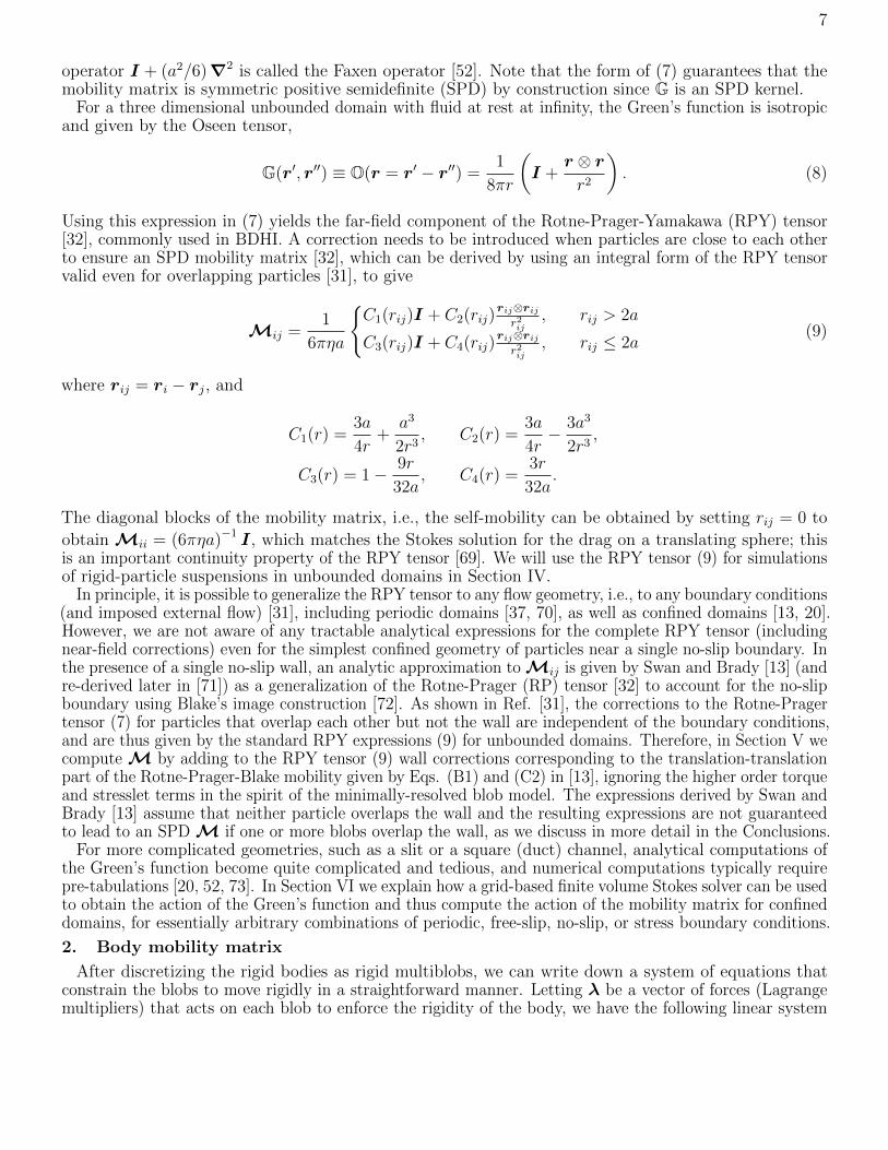
of spheres in an unbounded domain (e.g., clusters of colloids formed in a gel). For unbounded domains, wecompute the product of the blob-blob mobility matrixM with a vector using the Fast Multipole Method(FMM) developed specifically for the RPY tensor in [33]; this software makes four calls to the Poisson FMMimplemented in the FMMLIB3D library (http://www.cims.nyu.edu/cmcl/fmm3dlib/fmm3dlib.html)per matrix-vector product. As we will demonstrate empirically, the asymptotic cost of the rigid-multiblobmethod scales as Nb lnNb, where Nb is the total number of blobs, with a coefficient that grows only weaklywith density. We note that in this paper we use relatively tight tolerances (∼ 10−9 − 10−8) when computingthe matrix-vector products solving the linear systems in order to test the robustness of the preconditioners;in practical applications much lower tolerances (∼ 10−5 − 10−3) would typically be employed, potentiallylowering the overall computational effort considerably over what is reported here.

In this work, each sphere is discretized with n blobs of hydrodynamic radius a distributed on the surfaceof a sphere of geometric radius Rg. We discretize the surface of a sphere as a shell of blobs constructed by arecursive procedure suggested to us by Charles Peskin (private communication); the same procedure is used in[29]. We start with 12 blobs placed at the vertices of an icosahedron [35], which gives a uniform triangulationof a sphere by 20 triangular faces. Then, we place a new blob at the center of each edge and recursivelysubdivide each triangle into four smaller triangles, projecting the vertices back to the surface of the spherealong the way. Each subdivision approximately quadruples the number of vertices, with the k-th subdivisionproducing a model with 10 ·4k−1 +2 blobs, leading to shells with 12, 42, 162 or 642 blobs, see Fig. 2 in [68] foran illustration. In this section we study the optimal choice of a for a given resolution (number of blobs) and Rg.

An important concept that will be used heavily in the rest of this paper is that of an effective hydrodynamicradius Rh ≈ Rg + a/2 of a blob model of a sphere (more generally, effective hydrodynamic extent). Ifwe approach the rigid multiblob method from a boundary integral perspective, we would assign Rh = Rgas the radius and treat the additional enlargement of the effective hydrodynamic radius as a numerical(quadrature+regularization) error. This is more or less how results are presented in the recent work of Swanand Wang [29] (see for example their Fig. 8), making the accuracy appear low even in the far field for smallnumber of blobs per sphere. However, we instead think of a rigid multiblob as an effective model of a sphere,whose hydrodynamic response mimics that of an equivalent sphere. A similar effect appears in lattice Boltz-mann simulations, with a being related to the lattice spacing [94, 95]. To appreciate why it is imperative touse an effective radius, observe that even a single blob acts as an approximation of a sphere with radius a > 0.Similarly, one should not treat a line of blobs (see left-most panel in Fig. 1) as a zero-thickness object (line);rather, such a line of rigidly-connected blobs should be considered to model a rigid cylinder with finite thick-ness proportional to a [65]. We compute the effective hydrodynamic radius of our blob models of spheres next.

A. Effective hydrodynamic radii of rigid multiblob spheres

In this section we consider an isolated rigid multiblob sphere in an unbounded domain, and computeits response to an applied force fp, an applied torque τp, and an applied linear shear flow with strainrate γ. Each of these defines an effective hydrodynamic radius by comparing to the analytical resultsfor a sphere, therefore, each model of a sphere will have three distinct hydrodynamic radii.

The translational radius is measured from (see also [18])

Rh =fp

6πηup,

where up is the resulting sphere linear velocity, the rotational radius is (see also [18])

Rτ =

(τp

8πηωp

)1/3

where ωp is the resulting angular velocity, and the effective stresslet radius is

Rs =

(− 3s11

20πηγ

)1/3

.

Here we compute the stresslet s induced on the rigid multiblob under an applied shear by setting anapparent slip ui = −v(ri) = −γ(x,−y, 0) on blob i, and then solving the mobility problem to compute

19

the constraint (rigidity) forces λ. The stresslet s is the symmetric traceless component of the first momentof the constraint forces

∑i∈Bp λi ⊗ ri. In this work, we use Rh as the effective hydrodynamic radius when

comparing to theory. This is because the translational mobility is controlled by the most long-ranged1/r hydrodynamic interactions, and therefore the far-field response of a rigid multiblob is controlled by Rh.

Observe that since we only account for translation of the blobs, only Rh is nonzero for a single blob,while Rτ and Rs are zero. Therefore, the minimal model of a sphere that allows for nontrivial rotlet andstresslets is the icosahedral model (12 blobs) [35]. Since the rigid multiblob models are able to exert astress on the fluid they can change the viscosity of a suspension [35], unlike the single-blob models, whichdo not resist shear. It is important to note that the rigid multiblob models of a sphere are not perfectlyrotationally invariant, especially for low resolutions. Therefore, the rigid multiblobs may exhibit a smalltranslational velocity even in the absence of an applied force, or they may exhibit a small rotation evenin the absence of an applied torque. In other words, the effective mobility matrix for a rigid multiblobmodel of a sphere can exhibit small off-diagonal components. Similarly, there will in general be smallbut nonzero components of the stresslet that would be identically zero for a perfect sphere. In general, wefind these spurious components to be very small even for the minimally resolved icosahedral rigid multiblob.

A key parameter that we need to choose is how to relate the blob hydrodynamic radius a with the typicalspacing between the blobs. Since our multiblob models of spheres are regular the minimal spacing betweenmarkers s is well-defined, and we expect that there will be some optimal ratio a/s that will make therigid multiblob represent a true rigid sphere as best as possible. In a number of prior works the intuitivechoice a/s = 1/2 has been used, since this corresponds to the idea that the blobs act as a sphere of radiusa and we would like them to touch the other blobs. However, as we explained above, it is not appropriateto think of blobs as spheres with a well-defined surface, and it is therefore important to study the optimalspacing more carefully.

Number of blobs a/s = 1/2 a/s = 1/4Rh/Rg Rτ/Rg Rs/Rg Rh/Rg Rτ/Rg Rs/Rg

12 1.2625 1.2313 1.2461 1.0154 1.0292 0.989042 1.1220 1.1019 1.1316 1.0035 1.0147 0.9959162 1.0530 1.0472 1.0567 0.9998 1.0073 0.9968642 1.0239 1.0227 1.0250 0.9992 1.0036 0.99322562 1.0113 1.0111 1.0115 0.9994 1.0018 0.9986

φiterations

12 blobs 42 blobs

1.4 · 10−3 4 40.011 5 60.09 9 100.18 13 130.36 20 23

Table I: (Left) Effective translational, rotational and stresslet hydrodynamic radii for rigid multiblob models ofa sphere, for two choices of the blob-blob relative spacing a/s. (Right) Iterations to solve the mobility problem withtolerance 10−8 for 4096 spheres discretized with 12 blobs, or for 512 spheres discretized with 42 blobs, arrangedin a simple cubic lattice at different volume fractions φ, see Sec. IV D.

In the left half of Table I we present the effective sphere radii obtained for different resolutions for twochoices of a/s (we have investigated a broad range of spacings, not shown). The important observation wemake is that even when the radii are far from the geometric, such as for the 12-blob shell, the different radiiare rather consistent with each other. This means that even low-resolution rigid multiblobs act like spheresas far as low-order moments (multipoles) are concerned. We note that the method developed in [18], inwhich rotational degrees of freedom are added to the blob description, gives Rh ≈ Rτ to within a fraction ofa percent even for only 12 blobs per sphere. As the resolution is increased all hydrodynamic radii convergeto the geometric radius Rg linearly with a/Rg (data not shown). The table also suggests that a/s = 1/4is better than a/s = 0.5 because for a/s = 1/4 all of the effective hydrodynamic radii are remarkablyclose to Rg even for the 12-blob model. However, as we show in the next section, the choice a/s = 1/2is substantially better when looking at how well lubrication forces are resolved between two spheres.

B. Mobility for a pair of spheres

To determine the best value of a/s in this section we examine the hydrodynamic interaction betweentwo spheres as they approach each other. Since pairwise lubrication corrections are not added in ourapproach, it is important to investigate how well lubrication is resolved for different resolutions. To assertthe accuracy of the rigid multiblob models we will examine several non-trivial components of the mobilitybetween two spheres. Since rigid multiblob models are not rotationally invariant the exact value for the

20

pair mobility depends on the relative orientation of the rigid multiblobs; here we report the mean and(twice the) standard deviation of the particle velocity as error bars, averaged over a sample of randomorientations of the two particles. We note that we have compared our results to those obtained withthe method developed in [18], where rotational DOFs are included in the blob description, and foundonly a small difference (not shown). This means that the inclusion of blob torques does not lead to animprovement in the accuracy with which pairwise hydrodynamic interactions are computed.

In our first test, we pull two spheres toward each other with equal but opposite forces directed alongthe line of collision. In the top-left panel of Fig. 2 we compare the numerical results for spheres with162 markers and different blob radius a with the exact result derived by Brenner [96]. One can see thatfor long distances all sensible choices of a provide a good agreement with the exact theory once the resultshave been scaled with the hydrodynamic radius Rh computed in Section IV A. However, the choice ofa makes a big difference at short distances. Specifically, for small a/s flow can “leak” inbetween the blobsand the lubrication force is substantially lowered. For large a/s, we expect that the corrugation of theeffective hydrodynamic surface of the sphere will introduce deviations from a spherical shape. As thefigure illustrates, the best agreement between theory and numerical results is obtained for a/s = 1/2. Thisintuitive choice has been used in other related methods [5, 16, 63], while the IB community has favoredshorter distance between markers (but see discussion in Ref. [42]). In the rest of the tests on this sectionwe use a/s = 1/2 and in the rest of the paper we will use a/s ≈ 1/2 unless otherwise noted.

We explore the “lubrication” forces between spheres at very close distances in more detail in Fig. 3.In the left panel we show how the hydrodynamic force grows as the gap between the spheres decreases.The hydrodynamics of the low resolution models start to deviate from the theory for gaps ∼ Rh/2 orsmaller, while the highest resolution model (2562 blobs) shows a good agreement with the theory for gapsdown to 0.1Rh. The right panel of Fig. 3 shows the velocity error for one of the spheres with respect theexact theoretical result. For all models the error is below 10−3 until distances where the blobs forming thespherical shells start to overlap, which is the intuitive distance above which we expect the rigid multiblobto act as a good approximation to a sphere.

In our second test, we measure the velocity of one sphere located at the origin when a second sphere,located at (x, 0, 2Rh), is subject to an external torque applied around the x-axis. Since the Brenner theoryis only valid for spheres approaching along the line of collision we use the expansion of Jeffrey & Onishiaccurate to order O (r−100) [97] to compare with our mobility results; this expansion is also used in StokesianDynamics to compute near-field lubrication corrections for pairs of spheres and can be computed usingthe libStokes library of Ichiki [36]. One can see on the lower panels of Fig. 2 that the low resolution model(12 blobs) is similar to a Stokesian dynamics model that includes monopole (forces) and dipole (torques andstresslet) terms but no lubrication corrections. As the resolution of the models is increased the results agreebetter with the theory, as expected. Note, however, that the lack of lubrication corrections in our modelsprevents a perfect agreement down to contact distances. In the top right panel of Fig. 2 we comparethe stresslet computed on the particle at the origin. Again, we observe that the 12 blob model is similarin accuracy (aside from the presence of nonzero error bars, i.e., variance) to the Stokesian dynamic methodwithout lubrication corrections, while higher resolutions methods agree better with the theory, as expected.

C. Squirmer swimming speed

In this section we confirm the ability of our method to model an active sphere “squirmer” [4] with aprescribed tangential surface slip on the surface. This slip ui = u (ri) takes the following form in sphericalcoordinates,

ur = 0, uφ = 0, uθ = B1 sin θ

The active translational velocity of the squirmer is well-known to be the surface average of the surface slip [98],

u = −〈u〉 =2

3B1z.

We have numerically computed the swimming speed of a squirmer in an unbounded domain for differentresolutions and compared to the theory. We obtain that the relative error ε in the swimming speed islinear in a/Rg, which is expected. However, the error has a large prefactor, ε ≈ 3.5 a/Rg, which is notsmall for the low-resolution models. Furthermore, observe that linear convergence with the size of theblobs implies only order one-half convergence in the number of blobs since the number of blobs requiredto cover the surface of the sphere grows quadratically with the sphere radius.

21

2.00 2.25 2.50 2.75 3.00 3.25d / R

h

0.00

0.10

0.20

0.30

0.40

0.50

0.60

ux

x 6

πη

Rh

/ f

x

TheoryFTS1 bloba / s = 0.735a / s = 0.5a / s = 0.3a / s = 0.25

2.00 2.25 2.50 2.75 3.00 3.25d / R

h

-5

-4

-3

-2

-1

0

s yz

x

6π

/

τx

TheoryFTS12 blobs42 blobs162 blobs642 blobs2562 blobs

1.90 2.00 2.10 2.20 2.30 2.40 2.50d / R

h

0.10

0.15

0.20

vy

x 6

πη

Rh

2

/ τ

x

TheoryFTS12 blobs42 blobs162 blobs642 blobs2562 blobs

2.00 2.25 2.50 2.75 3.00 3.25d / R

h

-0.05

-0.04

-0.03

-0.02

-0.01

0.00

0.01

0.02

ωx

x 6

πη

Rh

3

/ τ

x

TheoryFTS12 blobs42 blobs162 blobs642 blobs2562 blobs

Figure 2: Hydrodynamic coupling between two identical spheres as a function of the center to center distanced. Twice the standard deviation as the two spheres are rotated relative to one another is shown as an error bar.Comparison is made to Stokesian dynamics without lubrication corrections, i.e., truncation at the FTS level, and to“exact” theory [96, 97], see legend. The top left panel shows the average sphere velocity under the action of externalunit forces f1 = −f2 = f directed along the line of collision, for a resolution of 162 blobs and for several valuesof a/s. The remaining three panels show non-trivial components of the pairwise mobility for a fixed a/s = 0.5and different resolutions (number of blobs per sphere, see legend). One sphere, located at

((d2 − 4R2

h

)1/2, 0, 2Rh

),

is subject to an external torque of magnitude one around the x-axis. The response of the second sphere locatedat the origin is measured: the top right panel shows the stresslet s (i.e., the rotation-stresslet coupling), the bottomleft panel shows the linear velocity (i.e., the rotation-translation coupling) v, and the bottom right panel showsthe angular velocity ω (i.e., the rotation-rotation coupling) of the second sphere.

These findings confirm that the rigid multiblob models converge to the correct swimming speed but the accu-racy is not very good. This is, in fact, not so surprising because we did not include any adjustments to accountfor the (potentially large) difference between the effective hydrodynamic radius Rh and the geometric radius.That is, even though the effective no-slip surface has a radius Rh > Rg, we imposed the slip (in a locally-averaged way) at the surface of a sphere of radius Rg. We will investigate these issues and potential ways to im-prove the accuracy with which active slip is imposed in future work. Here we simply note that rigid multiblobmodels are well-suited to qualitative studies of suspensions of many active particles. If one wishes to accuratelymodel one or a few active particles higher-order methods such as boundary integral methods are preferable.

22

0.01 0.1 1(d - 2R

h) / R

h

100

101

102

f x

/ (

6π

ιηR

hx u

x)

TheoryRPYFTS Truncation12 blobs42 blobs162 blobs642 blobs2562 blobs

2 2.5 3 3.5 4

d / Rh

10-6

10-5

10-4

10-3

10-2

no

rmali

zed

err

or

12-blobs

42-blobs

162-blobs

642-blobs

Figure 3: Lubrication forces on two identical spheres pulled toward each other with equal forces, for differentresolutions (see legend). Twice the standard deviation as the two spheres are rotated relative to one another isshown as an error bar. (Left panel) Dimensionless normalized hydrodynamic resistance, i.e., the inverse of thehydrodynamic mobility shown in the top left panel in Fig. 2. (Right panel) Velocity error for one sphere with respectthe exact theoretical result, normalized with the velocity at long distances (f/6πηRh). The distance d = 2 (Rg + a)at which blobs start to overlap is marked as a vertical line of the same color as the corresponding symbols.

D. Suspension of spheres

In this section we study the convergence of the preconditioned Krylov solver for suspensions of manyspheres. Our primary goal is to assess the effectiveness of our block-diagonal preconditioner for differentpacking densities (particle-particle distances) and numbers of particles. In the tests of this section weuse spherical shells of 42 blobs subject to random forces, torques and slips. We form a finite cubic subsetof a simple cubic lattice and place it in an unbounded fluid domain. We use right preconditioned GMRESwithout restarts, implemented using the PETSc [81] library.

First, we test the robustness with increasing system size, keeping the particles well-separated at a distance4Rg ≈ 3.6Rh, which corresponds to volume fraction φ ≈ 0.09. The left panel of Fig. 4 shows that theconvergence is uniform and that the number of iterations to reduce the residual by a given factor depends veryweakly on the number of spheres. This demonstrates the effectiveness of the block-diagonal preconditionerfor the mobility problem. Next we investigate the robustness with respect to packing density. The right halfof Table I shows the number of iterations to convergence for spheres arranged in a cubic simple lattice forseveral packing densities. When particles are far apart the solver converges fast because the hydrodynamicinteractions between particles are weak and the preconditioner is designed to be an exact solver for a singlebody. As the spheres come closer together the preconditioner is not so effective and the Krylov solver needsto perform more iterations, as expected. However, even when the particles are relatively close the solverperforms reasonably well. For example, when the spheres are at a distance of 2.55Rg ≈ 2.3Rh (φ ≈ 0.36), thesolver converges in 23 iterations. Of course, as the particles come closer and closer, and in particular, as theblobs on disjoint spheres begin to overlap, we expect to see an increasing ill-conditioning of the linear system(11) and an increasing number of iterations. However, the rigid multiblob method should not be used in thisregime, since it does not accurately resolve lubrication forces at such short distances. In the right panel ofFig. 4 we show the wall-clock time to solve the mobility problem for different number of shells and volumefractions. Since the number of iterations is essentially independent of the system size we obtain a quasi-linearscaling by using the FMM to compute the product between the blob-blob mobility matrix and a vector.

However, for the resistance problem explained in Sec. II, the left panel of Fig. 4 shows that the numberof iterations to attain convergence increase with the number of particles as N1/3, i.e., with the linear extentof the system. This is somewhat better than the O

(N1/2

)iterations reported for Stokesian dynamics

by Ichiki [36], but still much worse than the mobility problem.We believe that this difference between resistance and mobility problems is physical rather than purely

23

0 20 40 60 80

iteration

10-8

10-7

10-6

10-5

10-4

10-3

10-2

10-1

100

resid

ual

Mob. N=8

Mob. N=64

Mob. N=512

Mob. N=4096

Resist. N=8

Resist. N=64

Resist. N=512

Resist. N=4096

100

101

102

103

104

105

106

number of shells

10-1

100

101

102

103

104

105

tim

e (s

)

φ = 0.09, Plane-wave FMM

φ = 0.36, Plane-wave FMM

φ = 0.09, Multipole FMM

φ = 0.36, Multipole FMM

~ Nblog(N

b)

Figure 4: (Left panel) Convergence of preconditioned GMRES for the resistance and mobility problems for afinite subset of a cubic lattice of 42-blob spheres in an unbounded domain, for different number of particles, keepingthe lattice spacing (closest distance between spheres) at 4Rg ∼ 3.6Rh (corresponding to φ = 0.09). (Right panel)Wall-clock time to solve the mobility problem with a tolerance 10−8 versus the number of spherical shells fortwo volume fractions φ, demonstrating the O(Nb log(Nb)) asymptotic complexity, where Nb is the number of blobs.The matrix-vector product was computed with relative tolerance 0.5 · 10−9 using the FMM method developedin Ref. [33]. We compare the performance of a parallel multipole-based FMM3DLIB code [34] with a more efficientbut serial plane-wave FMM currently under development in the group of Leslie Greengard. Parallel runs used8 cores and serial runs used a single core of an Intel Xeon 2.40GHz processor.

numerical. In particular, we expect that the same behavior will be observed in essentially any other iterativemethod, regardless of the specifics of the discretization of the problem (rigid multiblobs, boundary-integralmethods, multipole expansions, regularized Stokeslets, etc.). To appreciate the difference between mobilityand resistance problems, observe that it is possible to obtain a low accurate solution to the mobilityproblem by approximating each sphere by a single blob and then computing the matrix vector productMf = u using an FMM. On the other hand, to solve the resistance problem the linear systemMf = uhas to be solved, which must account for the collective nature of hydrodynamic interactions. The differenceappears because there is an effective far-field two-body approximation for the mobility N (equivalentlyforM) but not for the resistance matrix N−1 (orM−1), which is essentially a multibody problem [99].

Mathematically, the difference appears because solving the saddle point problem (11) is similar tocomputing the motion for force- and torque-free particles [100], even though forces and torques are appliedon the particles. For force- and torque-free particles, the hydrodynamic fields and thus interactions withother particles decay faster than 1/r. Therefore, the effective interactions that need to be captured bythe iterative solver decay much faster for the mobility problem than for the resistance problem, makingthe former much easier. To confirm this intuition, we have studied (not shown) mixed resistance/mobilityproblems. When we fix the angular velocities but leave the linear velocities as free, we expect to see rapidconvergence because the leading order interactions that the Krylov method needs to capture decay as1/r3. Indeed, we observe numerically that in this case the solver converges almost as well as for the puremobility problem. However, when we fix the linear velocities of the spheres but let them freely rotate,we find that the solver converges almost as bad as for the pure resistance problem.

V. Results: Single Wall

In this section we study the accuracy of rigid multiblob models and the effectiveness of our block diagonalpreconditioner for particle suspensions sedimented near a single no-slip boundary. This is an importantand common occurrence in practice, especially in the field of active matter, since many active particleshave metallic components and are not density-matched with the solvent, and thus sediment to the bottomsubstrate. Some of us studied the diffusive dynamics of nonspherical particles near a no-slip boundary usinga rigid multiblob approach in Ref. [68]. However, in that prior work, we only studied a single body and

24

therefore all of the mobility matrices were simply formed as dense matrices. Here we explore in more detailthe accuracy of rigid multiblob models and also demonstrate how to scale rigid multiblob computationsto suspensions of thousands of rigid bodies.

To compute the hydrodynamic interactions between blobs in the presence of a single wall we use a pairwiseapproximation to the blobs’ mobility which includes the effects of the wall in the Rotne-Prager tensor [13]. Inour implementation, we compute the product of the blob-blob mobility matrixM with a vector using a directO(N2

b ) summation (here Nb is the number of blobs) implemented on a GPU using PyCUDA [101] in doubleprecision; single precision can be used for lower accuracy requirements. This is an ideal problem for usingGPUs as an accelerator since the computation is trivially parallelized on shared memory. Furthermore, thecommunication requirements between the CPU and GPU are minimal, since only the positions of the blobsneed to be communicated 4. It is possible to implement a fast multipole method (FMM) for the RP(Y) tensorincluding wall corrections by using a system of images together with an FMM for unbounded domains [33, 34].However, it is important to note that the asymptotically-optimal FMMs on a CPU (even with multicoreacceleration) will only be computationally more efficient than a direct sum on a GPU for more than about onehundred thousand blobs (in our testing on current hardware). Therefore, for many applications a simple GPUimplementation is sufficient or even preferable over an asymptotically scalable implementation. Our PyCUDAcodes are publicly available at https://github.com/stochasticHydroTools/RigidMultiblobsWall.Once a Rotne-Prager regularization of the construction of Gimbutas et al. [34] is developed and combinedwith an FMM, the asymptotic cost will be reduced to O(Nb logNb) and our computations can be extendedto millions of blobs.

In section V A we study the accuracy of rigid multiblob models for modeling a sphere close to a boundary,and in Section V B we extend this study to a rigid cylinder (rod). In section V C we study the dynamics ofa pair of active rods close to a no slip boundary. In section V D we study the performance of our iterativesolver on a suspension of many rods, and demonstrate that the number of GMRES iterations is essentiallyindependent of the number of particles just as for suspensions in an unbounded domain (see Section IV D).

A. Sphere

In this section the mobility µ ≡N of a rigid multiblob sphere whose center is at a distance H from a no-slip boundary is compared with some theoretical results available in the literature. We use the shell models ofspheres described in Sec. IV, and show the mean and standard deviation of the computed mobility averagedover a large number of random orientations of the rigid multiblob relative to the boundary. To denote thespecific component of the mobility matrix we use a subscript tt for translational mobility, rr for rotationalmobility and tr for translation-rotation coupling mobility, and we use a superscript ⊥ or ‖ to denote whetherthe direction of the force, torque, velocity or angular velocity is perpendicular or parallel to the wall.

The top left panel of Fig. 5 presents the translational mobility of the sphere perpendicular to the walltogether with the exact theory obtained by Brenner [96] (see also Eq. (D2) in [68] for a simple but accurateapproximation). We also compare to the complete expression for the Rotne-Prager-Blake tensor derivedby Swan and Brady [13], including stresslet corrections, which corresponds to an FTS truncation (plusdegenerate quadrupole corrections) of the multipole hierarchy. It is evident that a single-blob model ofa sphere, just like the substantially more complicated FTS truncation, does not recover the strong drop inthe mobility (i.e., lubrication) at small distances to the wall. Rigid multiblob models do substantially betterthan the FTS truncation even with only 12 blobs (icosahedral multiblob), and, as expected, the accuracyis improved with the addition of more blobs. As in the Sec.IV, the numerical mobility never goes exactly tozero since we do not add lubrication corrections, and we expect the rigid multiblob model to only work wellwhen the blobs do not overlap the boundary itself. In fact, we recall here that the RP tensor we use here[13] does not include near-field corrections when blobs overlap the wall, and therefore repulsive forces orother mechanisms should be used to ensure that the rigid multiblob is sufficiently far from the boundary. Weempirically observe that the rotational invariance gets violated strongly if the gap to the wall is less than 2a/3,which corresponds to 7% of the sphere radius for 12 blobs, and about 2% of the radius for the 642 blob model.

In the remaining panels of Fig. 5 we investigate other components of the mobility. There are no closed-formexpressions (even as infinite sums) for these components that are valid for all distances to the wall, so we usethe best approximations available, see Appendix D in [68] for specific formulas. For the translational mobility

4 For suspensions of identical bodies only the positions and orientations of the rigid bodies (so only up to 7 numbers per

body) need to be communicated to the GPU.

25

1.0 1.2 1.4 1.6 1.8 2.0H/Rh

0.0

0.1

0.2

0.3

0.4

0.5µ

⟂ tt/µ

0⟂

tt

TheoryFTS12-blobs42-blobs162-blobs642-blobs

1.0 1.2 1.4 1.6 1.8 2.0H/Rh

0.2

0.3

0.4

0.5

0.6

0.7

0.8

µ∥ tt/µ

0∥

tt

TheoryFTS12-blobs42-blobs162-blobs642-blobsfit

1.0 1.2 1.4 1.6 1.8 2.0H/Rh

0.3

0.4

0.5

0.6

0.7

0.8

0.9

1.0

1.1

µ⟂,∥

rr/µ

0⟂,∥

rr Theory parallelFTS parallelFTS perp12-blobs42-blobs162-blobs642-blobsfit

1.0 1.2 1.4 1.6 1.8 2.0H/Rh

0.00

0.02

0.04

0.06

0.08

0.10

µ∥ rt×(

6πηR

2 h)

FTS12-blobs42-blobs162-blobs642-blobsfit

Figure 5: Selected components of the mobility µ matrix for a sphere close to a wall, normalized by the correspondingbulk (unbounded domain) mobility µ0 where possible. Comparison of the rigid multiblob results (symbols) ismade to the best available theoretical results (solid black lines) and the FTS approximation used in Stokesiandynamics [13] (dashed and dashed-dotted lines). Empirical fits listed in Appendix D are shown with a dottedline. (Top left) Translational mobility µ⊥tt for a force applied perpendicular to the wall. (Top right) Translational

mobility µ‖tt for a force parallel to the wall. (Bottom left) Rotational mobility for a torque applied parallel (µ

‖rr,

filled symbols) or perpendicular (µ⊥rr, empty symbols) to the wall. (Bottom right) Rotation-translation coupling

mobility µ‖tr for force or torque parallel to the wall.

parallel to the wall, shown in the top right panel of the figure, we use a result based on lubrication theory [102](see Eq. (D3) in [68]) when the sphere is very close to the wall (H < 1.03Rh), and an approximation to orderO ((H/Rh)

5) for larger distances [103, 104] (see Eq. (D4) in [68]). It is clear that the rigid multiblob matchesthe theory for large distances but that the approximate theory is not very accurate for H . 1.5Rh sincethe rigid multiblob results are clearly converging to something slightly different. As for the perpendicularmobility, we see that the icosahedral model (12 blobs) is substantially more accurate than an FTS truncation.

Our results for the rotational mobilities, for torque applied either perpendicular or parallel to the wall,are shown in the bottom left panel of the figure and agree with the FTS results at large distances. Wesee slow but clear convergence of the rigid multiblob results for the translation-rotation coupling, shownin the bottom right panel of the figure. This component of the mobility is therefore most difficult tocapture accurately, as is evident from the fact that the FTS truncation does pretty poorly in this case.Since neither the FTS truncation nor the asymptotic lubrication results [102] are sufficiently accuratefor comparison to experimental measurements, we have empirically fitted our highest-resolution results

26

for the mobilities for which there are no exact theoretical expressions. We show the fits in Fig. 5 andgive details about the fits in Appendix D for the benefit of other researchers.

B. Cylinder

In this section, we consider a cylinder (rod) of length L = 2.12 and diameter D = 2R = 0.325 of aspect ratioα = L/D ≈ 6.35, mimicking the metallic rods studied in recent experiments [47], for three different levels ofresolution. The minimal resolution rigid multiblob has blobs placed in a row along the axis of the cylinder (atotal of 14 blobs), while in the more resolved models, a hexagon (86 blobs) or a dodecagon (324 blobs) of blobsis placed along the circumference of the cylinder to better resolve it, as illustrated in Fig. 1. We study differentcomponents of the mobility matrix µ ≡N ; to specify the direction of the force, torque, velocity or angularvelocity we use a subscript ⊥ or ‖ to denote whether the direction is perpendicular or parallel to the axes of thecylinder, respectively, and a superscript to denote whether the direction is perpendicular or parallel to the wall.

1. Bulk mobility

The first question that must be answered when constructing a rigid multiblob model of a given body is whereto place the blobs and how to choose their hydrodynamic radius, to match the effective hydrodynamic responseof the actual rigid body. Here we generalize the approach taken in Section IV A for spheres to a nonsphericalbody and show how to match the (passive) mobility of an actual rigid cylinder with a rigid multiblob model.Based on the results for spheres, for resolutions other than the minimally-resolved model we cover thesurface (similarly for the ends of the cylinder) of a cylinder uniformly with spheres keeping the spacingbetween blobs both around the circumference and the length of the cylinder uniform and fixed at a/s = 0.5.

Because there are no exact analytical results for the mobility of a cylinder even in an unbounded domain,we estimate the true mobility of the cylinder µ0 in an unbounded domain numerically. Specifically, we placethe blobs on the surface of a cylinder of length L and radius R (i.e., the true geometric surface of the actualrod we are modeling), and numerically compute the mobility for different resolutions. We then extrapolateto the limit a→ 0 using the two finest resolutions (86 and 324 blobs) based on our knowledge that theerror is linear in a. For the translation-translation mobility we obtain (µ0

tt)‖ × 4πηL = 3.404 (compare

to 3.295 from slender-body theory [105]) and (µ0tt)⊥ × 4πηL = 2.606 (compare to 2.619 from slender-body

theory [105]), while for the rotation-rotation mobility we get (µ0rr)⊥ × πηL3/3 = 1.212 (compare to 1.211

from slender-body theory [65]) and (µ0rr)‖ × πηL3/3 = 12.678, see the last row in Table II.

Our goal here is to match the bulk mobility µ0 of our rigid multiblob models to that of a true cylinderas close as possible. To do this, for the surface-resolved models (86 and 324 blobs), we place the blobson the surface of a cylinder of the same aspect ratio α = 6.35 but with the geometric radius Rg of thiscylinder allowed to be smaller than the geometric radius of the actual particle, while keeping the blobspacing a/s = 0.5. We then numerically optimize the value of Rg to minimize a measure of the errorwith respect to (extrapolated) mobility of a true cylinder, to obtain Rg/R = 0.90 for the 86-blob modeland Rg/R = 0.95 for the 324-blob model. For the minimally-resolved model, we empirically tune both thegeometric length (i.e., the distance between the centers of the two furthest blobs) to Lg = 0.914L and theblob radius to a = 1.103R while keeping the number of blobs fixed at Nb = L/R + 1 = 14 as suggested byBringley and Peskin [65]. Table II shows the resulting infinite-domain mobilities for each resolution alongwith the relative error compared to the extrapolated values for infinite resolution. We see a relative erroralways less than 2.5% even for the minimally-resolved model, except for rotation of the cylinder around itsown axis; recall that the minimally-resolved model cannot support a torque around the axis of the cylinder.

Resolution(µ0tt

)‖ × 4πηL

(µ0tt

)⊥ × 4πηL

(µ0rr

)⊥ × πηL

3/3(µ0rr

)‖ × πηL

3/3

14 blobs 3.422 (−0.53%) 2.612 (−0.23%) 1.216 (−0.31%) NA86 blobs 3.324 (2.35%) 2.541 (2.48%) 1.240 (−2.34%) 11.564 (8.79%)324 blobs 3.360 (1.29%) 2.588 (0.67%) 1.225 (−1.06%) 12.274 (3.19%)

∞ (extrapolated) 3.4040 2.6061 1.212 12.678

Table II: Nontrivial elements of the bulk mobility matrix for empirically-optimized rigid multiblob models ofa cylinder of aspect ratio 6.35, shown in the three left panels of Fig. 1. The value in the limit of infinite resolutionis extrapolated numerically (see main text) and reported in the last row. The percentages in parenthesis correspondto the error relative to the infinite resolution estimates.

27

2. Mobility for a sedimented rod

Having determined the geometric parameters for the rigid multiblob models based on motion in anunbounded domain, we now study the accuracy of the three different resolutions for a cylinder close toa no-slip boundary. We assume that the cylinder is parallel to the wall with the centerline of the rodat a distance H from the no-slip boundary.

Figure 6 compares the computed mobility coefficients to available theoretical and experimental results.As could be expected, the decrease in mobility when approaching the boundary is clearly underestimatedwith the minimally-resolved model. The left panel of the figure shows the translational mobilities. For µ⊥⊥,the higher resolutions are in good agreement with the experimental measurements of Trahan and Husseyfor a sedimenting rod with aspect ratio α = 5.05 [106]. Our numerical results also match well the theory ofJeffrey and Onishi [107] for an infinite cylinder when H < 2R . It is important to emphasize that our modelis significantly more accurate than slender-body theory near boundaries; the slender-body theory resultsfrom [105, 108, 109] (not shown here) are reasonably accurate only when H/R > 3.5 for aspect ratiosα > 9 [106]. The rotational mobilities of the rod are shown in the right panel of Fig. 6. For the rotational

mobility µ‖‖, all three resolutions are in good agreement with the theory of Jeffrey and Onishi [107] for

an infinite cylinder. For µ‖⊥ and µ⊥⊥, the minimally-resolved model shows substantial errors near the wall,

but the two higher resolution models agree with each other quite well over a broad range of distances.

µ‖

‖

µ‖⊥

µ⊥⊥

H/R1 2 3 4 5 6 7

µtt×4πηL

0

0.5

1

1.5

2

2.5

3

14 blobs

86 blobs

324 blobs

Theory, 2D

Experiment

µ‖

‖µ⊥⊥

µ‖⊥

H/R1 2 3

µrr/µ

0 rr

0

0.2

0.4

0.6

0.8

1

14 blobs

86 blobs

324 blobs

Theory, 2D

Figure 6: Mobility coefficients for a cylinder of aspect ratio α = L/ (2R) = 6.35 when it is parallel to the wall, as afunction of the height of the rod centerline H/R. The superscript of the mobility denotes the direction with respectto the wall, while the subscript denotes the direction with respect to the rod axis. (Left panel) Translational mobilitycoefficients µtt normalized by 4πηL as in [106]. The curves with circles corresponds to the formulas from Jeffrey andOnishi for an infinite cylinder near a wall [107]. The black squares correspond to the experimental measurements ofTrahan and Hussey for a rods with aspect ratio α = 5.05 [106]. (Right panel) Rotational mobility coefficients µrr nor-malized by the corresponding bulk value. The curve with circles corresponds to an infinite cylinder near a wall [107].

C. Active Rod Pair

In this section we apply the rigid multiblob method to a problem of recent experimental and theoreticalinterest: the dynamics of a pair of active “nanorods” that exhibit a “pusher” or extensile dipolar flow atlarge distances. Specifically, we compute the motion of a dimer of tripartite nanorods, as studied in recentexperiments by Wykes et al. [47]. The rods have diameter of 0.325µm and length of 2.12µm, and arein force and torque equilibrium (under the action of gravity and Van der Waals and electrostatic interactionforces with the boundary) at some distance from the wall that has not been measured in the experiments.The rods are constructed of three metal sections, in the arrangement gold-platinum-gold (Au-Pt-Au) andcreate a dipolar extensile (pusher) far-field flow. As such, they do not propel themselves in isolation butexperiments show the formation of dimers of rods that actively rotate in a direction that is opposite of

28

that predicted by recent simulations [6], which neglect the presence of the bottom wall. In agreement withthe experiments, our simulations show the formation of a stable rod pair that touch each other tangentiallyand rotate (without exhibiting a significant translation) around an axis perpendicular to the wall in adirection consistent with the experimental measurements.

The exact details of the active flows near the surface of the rods have not been measured experimentallyand are difficult to predict analytically because this requires resolving the thin slip boundary layer (ofthickness related to the Debye length) around the rods, as well as the knowledge of a number of materialconstants that are not known accurately. To obtain a qualitative understanding of the dynamics of therods we impose an apparent tangential surface slip velocity on the two gold sections, directed away fromplatinum center and having a magnitude of 20µm/s; no slip is imposed on the platinum section. Note thatboth gravity and the active slip pull the rods toward the wall, so we use an ad hoc repulsive force with thewall to balance the distance between the cylinder centerline and the wall at one cylinder diameter. Due toelectrostatic interactions, a stacking of the two rods with the gold end of one rod aligned with the platinumcenter of the other is observed experimentally [47]; here we study the flow around such a pair of aligned rods.

Figure 7: Active flow around a pair of extensile nanorods composed of three segments (shown with blue, greenand red colors) sedimented on top of a no-slip boundary (the plane of the image) and viewed from above forthe three different levels of resolution illustrated in Fig. 1: minimally resolved (left), marginally resolved (middle),and well resolved (right). The colored disks (red, blue or green) are projections of the blobs, with no-slip conditionson the green blobs and active slip of magnitude 20µm/s on the blue and red blobs, directed away from the greensegment. A cut through the flow field is shown in the lab frame as a vector field along with streamlines, withthe magnitude of the velocity shown as a color scale plot.

In Fig. 7 we show the instantaneous flow around a dimer of active rods, as computed using the proceduredescribed in Appendix B and seen from above, for three different resolutions: a minimally-resolved, amoderately-resolved and a well-resolved model. The imposition of the slip at the surface of the blobsbecomes more and more accurate as the resolution is improved; however, we see a rather good matchbetween the three flow fields even relatively close to the rods and wall. Our simulations, which correctlytake into account the physical boundary conditions, estimate the angular frequency of rotation of the dimerto be approximately 0.64Hz in the counter-clockwise direction, consistent with experimental observations[47]. The estimated angular velocities are 0.62, 0.67 and 0.63Hz for each resolution respectively. We willstudy the dynamics of active nanorods near a no-slip surface in more detail in the future; in the nextsection we demonstrate that the calculations above can be scaled to suspensions of thousands of rods.

D. Suspension of rods near a boundary

In this section we test the efficiency of the preconditionner outlined in Section II B on a suspension of activerods sedimented near a wall. We have already seen that the block-diagonal preconditioner is able to accountfor the hydrodynamic interactions among the particles in a modest number of iterations for unbounded flow.Here we show that this continues to hold even when the wall strongly dominates the hydrodynamics, andinvestigate how important it is for the preconditioner to know about the presence of the boundary. Namely,

recall that in the block-diagonal preconditioner the diagonal blocks of M correspond to the blob-blob

mobility for an individual rod in the presence of the boundary. Since M depends on the configuration of each

29

rod relative to the wall, unlike for an unbounded suspension, all diagonal blocks need to be factorized anewfor each new configuration. However, it is also possible to use an approximate block diagonal preconditionerthat assumes an unbounded suspension, i.e., neglects the presence of the boundary when computing ablock-diagonal approximation of the blob-blob mobility. This seems like a strong approximation to bemade for objects close to a no-slip wall; however, the investigations below will demonstrate that the Krylovsolver can account not only for the rod-rod interactions, but also for the rod-wall interactions. This isan important finding because we recall that in the Green’s-function-free method described for confinedsuspensions in Section III, the boundary conditions are completely ignored in the preconditioner.

In these tests we discretize cylinders of aspect ratio α = L/D ≈ 6.4 either by placing 98 blobs on the surfaceof a cylinder of geometric length Lg = L and geometric radius Rg = 0.863R, keeping a/s = 0.5, or, by placing21 blobs of radius a = 1.02R uniformly spaced along a line segment of length L. For testing purposes, wegenerate random periodic packings of Nr rectangles at a surface packing density φa using a molecular dynamicscode [110]. We then use these hard-rectangle packings to generate a configuration of non-overlapping cylindersthat are parallel to the wall and at a constant distance H from the wall; we do not expect to see differentresults if some randomness is added to the heights and orientations of the cylinders relative to the wall, aslong as their surfaces remain sufficiently far from the wall. In our tests we vary the centerline height H fromH = 0.75D to H = 2D, the area fraction φa from 0.01 to 0.6, and the number of rods Nr from 10 to 104; thenumber of blobs varies in the range from Nb = 200 to about Nb = 106. For our implementation and hardware(a Tesla K20 GPU) one GMRES iteration takes around 0.3s for Nb = 104, 1s for Nb ≈ 2·104, 20s for Nb ≈ 105,and 220s for Nb ≈ 3 ·105; we emphasize again that by using an FMM one can change the scaling from O (N2

b )to O (Nb logNb) and thus substantially reduce the computational times for large Nb, see right panel in Fig.4. To ensure a nontrivial right hand side of the linear system when testing the iterative solver, each blob isprescribed a random slip velocity and a random force, producing a random force and torque on each cylinder.

The left half of Table III shows the scaling of the number of GMRES iterations with the area fractionφa for a fixed number of rods Nr = 1000, and compares the efficiency of the preconditioner using thefull (wall-corrected) to that using the approximate (no wall contributions) block-diagonal preconditioner.We observe that the number of iterations increases slowly with the area fraction for both resolutions andreaches a maximum of 31 iterations for φa = 0.6 with the wall-corrected preconditioner. Therefore, aswe already saw in Section IV D, the performance of the preconditioner is not highly sensitive to near-fieldinteractions. When using the approximate block-diagonal preconditioner without the wall corrections, thenumber of iterations is increased, as expected. However, this increase never exceeds 50%, which means thateven a poor approximation of the mobility can be used in the preconditioner in practice. The right halfof Table III shows the scaling of the preconditioner with the number of rods Nr for a fixed area fractionφa = 0.1. The number of iterations rapidly saturates around 20 and becomes independent of the numberof rods for both resolutions and heights. This confirms that the results obtained for a suspension of spheresin Section IV D apply to confined suspensions as well. Note that for the largest system sizes studied inthe right half of Table III a linear-scaling FMM implementation would likely be substantially more efficientthan the quadratic-scaling GPU implementation employed here.

VI. Results: Confined Domains

In this section, we numerically explore the accuracy and efficiency of the rigid multiblob immersed boundary(IB) method described in Section III. This method is suited to fully confined (bounded) domains, and here wemodel suspensions of spheres in a periodic domain, a slit channel (i.e., two parallel walls), and a square (duct)channel. As discussed in more detail in Section III, for periodic suspensions it is possible to use FFT-basedmethods [25, 30, 38, 45] to obtain the product of the blob-blob mobility matrix with a vector. Future workshould compare the method developed here with such approaches, especially for Brownian suspensions.

The effective hydrodynamic radius of an IB blob (also called a “marker” or “IB point” in the IB literature[83]) can be computed numerically by dragging a single blob with a constant applied force through a largeperiodic grid with spacing h and applying the Hasimoto periodic correction [41, 43]. When averaged overmany positions of the marker relative to the underlying grid, for the six-point kernel [88] used here 5 we obtaina ≈ 1.47 h. The geometry of the rigid multiblob models of a sphere used here is the same as in Sections IV andV. We also know from Section IV B that the spacing between the blobs should be around s ≈ 2a ≈ 3h, which

5 As summarized in Refs. [41, 43], a ≈ 1.25h for the widely used four-point kernel [83], and a ≈ 0.91h for the three-point

kernel [111].

30

φa Resolution Wall-corrected Unbounded

0.0121 12 1798 16 28

0.121 19 2398 22 32

0.221 20 2598 23 34

0.421 25 2998 27 33

0.621 30 3398 31 43

Nr ResolutionH/D = 0.75 H/D = 2

iterations time (s) iterations time (s)

1021 7 0.15 7 0.1598 8 1.49 9 1.51

10021 14 1.95 13 1.5298 19 18.9 18 35.6

100021 19 32.7 16 29.898 22 620 20 559

500021 18 520 16 4,50098 23 10,200 22 12,400

1000021 20 2,050 17 1,43098 23 39,400 21 36,300

Table III: (Left) Number of GMRES iterations required to reduce the residual by a factor of 108 for several surfacepacking fractions and two different resolutions (number of blobs per rod), for H/D = 0.75 and Nr = 1000 rods. Thefull block-diagonal preconditioner, which takes into account the wall corrections for each body, is compared to the ap-proximate preconditioner, in which all wall corrections are neglected. (Right) Number of iterations and wall-clock time(using a direct GPU matrix-vector product on a Tesla K20 GPU) to solve the mobility problem with tolerance 10−8

using the wall-corrected preconditioner at φa = 0.1, for different number of rods and proximity of the rods to the wall.

is somewhat larger than the spacing s ≈ 2h used in [42], and leads to improved conditioning of the blob-blobmobility matrix. In fact, we observe that when distinct blobs overlap, the preconditioned GMRES solver de-scribed in Section III C shows significantly worse performance than when the blobs are not overlapping (or justtouching). We therefore recommend using s ' 3h for rigid multiblob suspensions at zero Reynolds numbers.

Determining the exact spacing is somewhat of an art and is problem specific. In the IB approach developedhere, the fast multipole method used in Section IV and the GPU matrix-vector product used in Section Vare replaced by a geometric multigrid method, which works best for grid sizes that are powers of two. Oncethe exact spacing is determined, the effective hydrodynamic radius of the rigid multiblob can be determinednumerically; we get very similar results for the IB method to those for an unbounded domain in Section IV A,after setting a = 1.47 h. For confined suspensions, the ratio of the size of the particles to the domain size istypically fixed to some experimental value, and this constrains the choice of number of grid cells and spacingbetween the blobs. In all of the tests presented here, we have empirically optimized the appropriate value forthe grid size and the spacing s in the interval 2h to 3h, and report the chosen values. As explained earlier,it is possible to use split IB kernels to gain more flexibility in choosing the grid sizes and blob spacing.

In Section VI A, we investigate in more detail the loss of perfect translational and rotational invariance of theblob-blob mobility and the mobility of rigid multiblob spheres, and demonstrate that by using the improvedsix point kernel [88] our method is able to minimize the grid artifacts to a significant extent. Note, however,that there is an additional loss of rotational invariance for rigid multiblob models that comes from discretizingthe bodies using blobs; this unphysical bias exists even in the absence of a fluid grid. In Section VI B weexplore in more detail the accuracy for different resolutions for a periodic suspension of spheres by comparingto reference results from multipole-based methods. In Section VI C we compute the mobility of a sphere ina slit channel and compare to existing theories for a number of resolutions. In Section VI D we compute theeffective quasi-two-dimensional diffusion coefficient of a boomerang colloid in a slit channel, and compare torecent experimental measurements [48, 49, 112]. In Section VI E we optimize the convergence of the iterativelinear solver for suspensions of many bodies, and demonstrate that the number of GMRES iterations isessentially independent of the number of particles, even in confined domains such as slit channels. Finally,we study the sedimentation velocities in a bidisperse suspension of spheres in Section VI F, and compare torecent Stokesian Dynamics simulations [38, 50]. In Appendix C we study flow around permeable rigid bodies.

A. Translational invariance

As explained in detail in Section III, for sufficiently large domains the blob-blob mobility computed bythe IB method has the approximate form (22). Deviations from this formula arise because of the imperfecttranslational and rotational invariance due to grid artifacts. The two functions f(r) and g(r) are expected tobe similar to those appearing in the RPY tensor (9). We obtain the actual form of the functions f(r) and g(r)

31

empirically by fitting numerical data for the parallel and perpendicular mobilities of a pair of blobs placedin a large periodic domain, see [42] for more details. The results are shown in the left panel of Fig. 8, andare compared to the RPY tensor for spheres of radius a = 1.47h. We have empirically fitted the numericalresults for f(r) and g(r) with a fit that has the proper asymptotic behavior at large and short distances,see Appendix A in [42] for more details; this fit is used in the preconditioner as an analytical approximationof the diagonal blocks of the blob-blob mobility matrix. We see that the differences between the fits andthe RPY tensor are rather small, and also confirm the improved translational invariance of the six-pointkernel [88] as evidenced in the small scatter of the points around the fits. This confirms our expectationthat the rigid multiblob IB method will behave similarly to an RPY-based method in terms of accuracy.

10−1

100

10−7

10−6

10−5

10−4

a/Rh

σµ

σ(µtt)/ < µtt >

σ(µrr)/ < µrr >

σ(µrt)/ < µtt >

σ(µttoff−diag)/ < µ

tt >σ(µrr

off−diag)/ < µrr >

a/Rh

Figure 8: Translational and rotational invariance of the rigid multiblob IB method. (Left panel) Empirical valuesof the blob-blob mobility functions f(r) and g(r) appearing in (22), normalized by 8πηr so that they asymptoteto unity. An empirical fit through the data is compared to the RPY tensor for blob radius a = 1.47h. Notethat the scatter around the fit for r & 5a is dominated by periodic artifacts due to the finite size of the grid.(Right panel) Standard deviations of the diagonal (translation-translation, rotation-rotation) and cross-coupling(rotation-translation) components of the mobility matrix for spheres discretized with 12, 42, 162 or 642 markersshells (i.e., for decreasing a/Rh). Also shown is the typical magnitude of the off-diagonal components of thetranslation-translation and rotation-rotation mobility matrices, which should be zero for a perfect sphere.

In the right panel of Fig. 8 we investigate the translational and rotational invariance of rigid multiblobmodels of spheres as a function of the resolution. We randomly move and rotate a sphere relative to theunderlying grid and compute the elements of the mobility matrix. The mean of these elements definesan effective translational and rotational radius consistent with the results presented in Section IV A (notshown). In the figure we show the normalized standard deviation of the elements of the mobility matrixas a function of the resolution (number of blobs). As expected, the normalized standard deviation decreaseslinearly with the size of the blobs a (equivalently, the inverse of the square root of Nb), and is below 10−4

for all mobility elements even for the 12-blob (icosahedral) model [35].

B. Periodic Suspension of Spheres

In this section we apply our rigid multiblob method to a benchmark resistance problem in a periodicsuspension of 108 spheres moving with random linear and angular velocities. This benchmark was developedby Anthony Ladd, who supplied us with a random and a face-centered cubic (FCC) configuration ofspheres, at a low density of φ = 0.05, as well as a high density of φ = 0.45. He also supplied to us theresults for the resulting forces and torques obtained using the HYDROMULTIPOLE code [54]. Note thatpairwise lubrication corrections have been included in the multipole expansion method used for thesecalculations [54, 56, 57]; to our knowledge no method has accounted for three-body lubrication corrections.

The rigid multiblob models used in this study have been chosen to give a blob spacing close to s ≈ 2a ≈ 3h,while ensuring that the number of grid cells is integer given the specified unit cell length in the benchmarkconfigurations, and to have a specified effective hydrodynamic radius Rh ≈ 1 for five different resolutions:a single blob per sphere (similar to a truncation with only one monopole per sphere), 12 blobs (geometricradius Rg = 0.7896, grid spacing h = 0.2778), 42 blobs (Rg = 0.8899, h = 0.1667), 162 blobs (Rg = 0.9502,

32

h = 0.08929) and 642 blobs (Rg = 0.9766, h = 0.0463) per sphere. The results for the x component of thecomputed forces on the spheres are illustrated in Fig. 9; similar results are observed for other components.

0 27 54 81 108sphere number

-60

-40

-20

0

20

40

60

80

f x

1-blob12-blobs42-blobs162-blobsMultipole (L=8)

SD

0 27 54 81 108sphere number

10-4

10-3

10-2

10-1

100

∆f x

/

<|f

x|>

1-blob12-blobs42-blobs162-blobs642-blobsSD

Figure 9: Results from the rigid multiblob method applied to Ladd’s benchmark resistance problem (with specifiedrandom velocities) for a periodic suspension of 108 spheres. (Left panel) The x-component of the force oneach sphere in a random suspension at a low volume fraction φ = 0.05. For comparison, we show the resultsof Stokesian dynamics (SD) [36] and the HYDROMULTIPOLE code [54] with L = 8 moments retained. Twoparticles that happen to be at a distance closer than 2.02 radii from each other are marked by a black box anda blue circle, and develop unresolved strong lubrication forces between them. (Right panel) The normalized error∣∣∣fx − f (ref)

x

∣∣∣ /〈∣∣∣f (ref)x

∣∣∣〉 in the x-component of the force for an FCC lattice at the high volume fraction φ = 0.45.

The HYDROMULTIPOLE code with L = 8 moments is used as a high-accuracy reference calculation.

In the left panel of Fig. 9, we focus on the low density suspension (φ = 0.05) and compare the forcescomputed by the rigid multigrid method with those computed using L = 8 multipole moments, as well as theresults of the Stokesian dynamics (SD) code of Ichiki [36] (which roughly corresponds to L = 2 moments).The overall agreement is quite good, but notice that even with 162 blobs per sphere we do not resolve thelubrication force between particles numbered 48 and 103, marked in the figure, since this pair of particles havea gap of only 0.024 radii between them. This is not surprising given that we do not include pairwise lubricationcorrections in our method; such corrections are included in the reference results we are comparing to so theyproduce accurate forces for all particles. In the rigid multiblob method, we resolve the near field interactionsmore and more accurately as we increase the number of blobs per sphere, but we cannot accurately resolvethe hydrodynamic interactions between pairs of particles with overlapping blobs (see Fig. 2).

At the high packing fraction φ = 0.45 there are many pairs of nearly touching particles in a typical randomsuspension of hard spheres in the absence of (electrostatic) repulsive forces, and there is no hope that the rigidmultiblob method can accurately compute the interparticle forces 6. Therefore, at this density we focus on anFCC lattice configuration, and compare to the multipole-based code with L = 8 moments. Here the closestparticle distance is 2.36 radii and our method is able to resolve the forces relatively well, especially with morethan 12 blobs per sphere, see the right panel in Fig. 9. This is perhaps not surprising; however, the moreimportant point we wish to make is that the SD results are now not significantly more accurate than the resultsobtained from using only a single blob per sphere. The addition of stresslets and pairwise lubrication doesnot appear to help much in resolving the many-body far field hydrodynamic multiple scattering in this latticeconfiguration. Using an icosahedral rigid multiblob already provides an order of magnitude improvement in

6 The results from HYDROMULTIPOLE suggest that even L = 15 moments, which is the maximum that could be afforded

with 32GB of memory since the linear system to be solved is dense and has about 7 · 104 unknowns, convergence is not

achieved to sufficiently high accuracy for the random suspension at φ = 0.45.

33

the typical error over an FTS truncation, and provides an error comparable to keeping L = 3 moments in theHYDROMULTIPOLE method (not shown), which is also the minimum number of moments necessary to keepto capture all long-ranged hydrodynamic interactions, as well as to model active sphere suspensions [2, 8].

C. Sphere in a slit channel

In this section we compute the parallel and perpendicular translational mobilities of a sphere in a slitchannel of thickness 19.2Rh as a function of the height H of the sphere center above one of the walls.This problem is of relevance to a number of experiments involving spherical colloids confined between twoglass microscope slips, and has also been used as a benchmark problem for boundary integral calculationsin [26]. Since the immersed boundary method used here cannot be used for infinite domains, we takea domain of dimensions (76.8, 19.2, 76.8)Rh and apply no-slip conditions on the y boundaries and periodicconditions in the other two directions.

There are no manageable theoretical results accurate for all distances from the wall and all channeldimensions [20]. For the parallel component of the mobility, Faxen obtained exact series expansions for themobility at the half and quarter channel locations, which we use to benchmark our calculations, neglectingthe corrections coming from the use of periodic boundary conditions in the directions parallel to the walls.For other positions of the sphere we employ the Modified Coherent Superposition Assumption (MCSA)approximation given in Eq. (9) in Ref. [113], with the mobility relative to a single wall given by the sametheoretical lines shown in Fig. 5. The rigid multiblob models used in this study have been chosen to give a blobspacing close to s ≈ 2a ≈ 3h, while ensuring that the number of grid cells is integer given the target channelwidth relative to the effective hydrodynamic radius of the sphere Rh for all of the resolutions studied: a singleblob as a minimal model of the sphere [41] (grid size 128×28×128), 12 blobs (grid size 256×64×256, geometricradius Rg = 2.503h, giving spacing s/h = 2.63), and 42 blobs (512×128×512 grid, Rg = 6.047h, s/h = 3.30).

0 1 2 3 4 5 6 7 8 9 10

H / Rh

0.0

0.2

0.4

0.6

0.8

1.0

µtt

⊥,

|| / µ

tt

0

⊥,||

1 blob

12 blobs

42 blobs

0.8 1 1.2 1.4 1.6 1.8 2

H / Rh

0.0

0.1

0.2

0.3

0.4

0.5

0.6

µtt

⊥,

|| /

µtt

0 ⊥

, ||

Figure 10: Translational mobility of a sphere in a slit channel of width 19.2Rh relative to the bulk, for severalresolutions of the rigid multiblobs (see legend), for forces/motion parallel (filled symbols) and perpendicular (emptysymbols) to the wall. The numerical results are in good agreement with the exact results of Faxen for distancesH = L/4 and H = L/2 (orange crosses). The inset shows that close to the wall the results for the 12 and 42blob shells are in reasonable agreement with the approximate MCSA theory (lines).

34

We have already confirmed that our results are in agreement with Faxen’s theory in the (extrapolated)limit of an infinitely long channel in our prior work [42]. Here we examine the mobility as the sphere movesthrough the channel, and in particular, as it comes close to the wall. The results of our calculations are shownin Fig. 10, and are in good agreement with the approximate MCSA theory for the parallel mobility. Notethat the MCSA theory is approximate even far from the wall, as seen from the fact that our results do notmatch it for the perpendicular mobility even at the center of the channel. The boundary condition handlingdescribed in Appendix D of [42] ensures that for a single blob the mobility vanishes at the boundary, i.e., forH = 0, rather than for H = Rh as for a true sphere. The more resolved models, however, do show a sharpdrop in mobility when the sphere nearly touches the wall. The inset shows that the lubrication interactionsare not resolved very close to the wall, just as we observed for a single wall in Section V A. Nevertheless,we note that unlike the Rotne-Prager-Blake mobility tensor computed by Swan and Brady [13] and usedin Section V A, the mobility computed by the grid-based Stokes solver is physically realistic even whenthe blobs overlap the wall. This has two important implications. First, the rigid multiblob IB method doesnot run into singularities for Hmin < H < Rh, where Hmin is the distance at which the center of some blobfirst leaves the physical domain. This is particularly beneficial in Brownian simulations, where stochasticmotion can push the sphere to slightly overlap the wall [41, 68]. Furthermore, the immersed boundaryresults in the inset of Fig. 10 are substantially more rotationally-invariant as the sphere approaches thewall than the corresponding results in the top two panels of Fig. 5; the error bars in the mobility due todiscretization artifacts are very small for the immersed boundary method even for H < Rh.

D. Boomerang in a slit channel

In this section we study the diffusion of a boomerang colloidal particle in a narrow slit channel, asrecently studied experimentally and theoretically [48, 49, 112]. The boomerangs are confined to essentiallyremain in the plane parallel to the wall by the tight confinement, and thus perform quasi two-dimensionaldiffusion. We previously studied the diffusion of such a boomerang colloid sedimented against a singleno-slip boundary in [68], using a strong gravitational force to keep the boomerang in quasi two dimensions.However, the colloids in the actual experiments are almost neutrally buoyant and a slit channel is usedto confine them to two dimensions. Here we use our rigid multiblob IB method to determine the effectivetwo dimensional diffusion coefficients of a single boomerang in slit confinement.

As discussed in detail in [68], it is, in principle, necessary to perform long Brownian simulationsto determine the long-time diffusion tensor D of nonspherical particles. However, if the mean squaredisplacement (MSD) is linear in time, the long and short-time time diffusion coefficients are equal andcan be obtained from the Stokes-Einstein relation

D = kBT 〈N 〉 = kBT µ, (29)

where µ is the average mobility over configurations following the Gibbs-Boltzmann (GB) distribution.Therefore, the diffusion coefficient can be computed by generating samples from the GB distribution ofboomerang configurations, and then solving a mobility problem for each configuration and averaging overthe samples. For quasi two-dimensional diffusion the MSD can be made nearly linear by a careful choice ofthe tracking point [48, 49, 68], which is the point whose translation is measured and around which torquesare expressed [114]. Chakrabarty et al. [48] have shown that for particles diffusing in two dimensions,the optimal choice of tracking point is the center of hydrodynamics stress (CoH), the location of whichcan be computed from the bulk mobility tensor [68].

To compare with the experimental results of Chakrabarty et al. we compute the diffusion coefficientof a single boomerang colloidal particle between two walls. In the experiments [48], colloidal particleswith boomerang shape diffuse in a channel of width ∼ 2µm. The boomerang particles, produced byphotolithography, have two arms of length 2.1µm, thickness 0.51µm and width 0.55µm forming a rightangle. In our computations, we use no-slip boundary conditions on the walls of the channel and periodicboundary conditions in the directions parallel to them. We construct two rigid multiblob models ofsuch boomerangs (see [68] for geometric details): a minimally resolved model with 15 blobs (grid size128 × 9 × 128, blob spacing s/h = 1.36) that is essentially a bent version of the cylinder model shownin the left-most panel of Fig. 1, and a moderately resolved model with 120 blobs (grid size 256× 18× 256and blob spacing s/h = 2.22), shown in the right-most panel of Fig. 1.

We assume a hard-core potential between each of the blobs and the walls, and average the mobility over100 samples generated from the Gibbs-Boltzmann distribution using an accept-reject Monte Carlo procedure

35

[68]. In the experiments, there is likely an additional electrostatic repulsion from the wall; we have checkedthat adding a short-ranged Yukawa-type repulsion with the walls does not change our results significantly 7.Following [48], we report the diffusion coefficients computed using (29) in the continuous body frame (CoB)[48] attached to the colloidal particle, such that the axis X1 goes along the line that bisect the boomerangangles and the axis X2 is orthogonal to X1 (see Fig. 1 in [48]). The diffusion coefficient for the boomerangparticle are given in Table IV. We see that the computed location of the CoH is in good agreement withexperimental estimates. However, both translational and the rotational in-plane diffusion coefficientscomputed in the simulations are twice larger than those measured experimentally, for both resolutions.

Experimentsratio = (Experiment / Simulation)15 blobs 120 blobs

d 1.16 (µm) 1.06 1.06D11 0.049 (µm2/s) 0.55 0.47D22 0.058 (µm2/s) 0.50 0.46

Dθ 0.044 (rad2/s) 0.46 0.46

Table IV: Comparison of experimentally-measured diffusion coefficients for a boomerang particle in a slit channelto numerical estimates obtained from the rigid multiblob IB method. The tracking point is chosen to be theCoH, which is a point on the boomerang bisector line at a distance d (first row) from the crossing point of thetwo boomerang arms. We report the translational diffusion coefficients D11 and D22 in the Continuous BodyFrame (CBF) of reference as in Ref. [48], averaged over 100 samples from the Gibbs-Boltzmann distributionof particle configurations, for two different resolutions.

To investigate this large mismatch between simulations and experiments, we explore further the differencebetween the right angle boomerangs used in the two distinct experiments [48] (arms of length 2.1µm andwidth 0.55µm) and [112] (arms of length 2.33µm and width 0.7µm), both for a reported channel width of 2µm.The boomerangs in [112] are reported to be about 10% larger than those used in [48]; however, the reporteddiffusion coefficients are reported to be about 25% larger. This is inconsistent with a purely hydrodynamicmodel, since the larger particles should have smaller bulk diffusion coefficients and are more confined.Therefore, the larger particles must have a translational diffusion coefficient that is more than 1.1 times smallerfor translation, and more than 1.13 ≈ 1.33 times smaller for rotation, if particle size is the only differencebetween the two experiments. Indeed, in our simulations the translational diffusion coefficient is about 1.25times smaller for the larger particles, and the rotational one is 1.57 times smaller. This suggest that there aresome unreported experimental effects that are not taken into account in the simulations, such as a potentiallynon-uniform channel thickness or polydispersity in the particles. More careful future investigations arerequired to understand the origin of the difference between simulations and experiments reported in Table IV.

E. GMRES convergence

In this section we investigate the performance of the preconditioner described in Sec. III C and determine

an optimal value for N(1)s and N

(2)s , the number of iterations in the first and second approximate Stokes

solves in the preconditioner. As a Krylov solver, here we use the restarted right-preconditioned GMRESmethod, but we have also observed good performance with the short-term recurrence BiCGStab method,which typically requires a few more iterations than GMRES but has smaller memory requirements. It isimportant to emphasize that the exact number of iterations depends strongly on the geometry of the rigidmultiblobs, notably, the spacing between the blobs. The performance depends even more strongly on theefficacy of the geometric multigrid preconditioner for the Poisson equation, which in the implementation usedhere is strongly degraded for grids that have a nearly prime number of cells in each dimension, and for gridsof large aspect ratios (even if all directions are powers of two). Our focus here is on investigating the trendsin the number of GMRES iterations with the various parameters in the preconditioner and the system size.

The computational cost of the solver is dominated by the application of the full preconditioner, whosecomplexity depends on nontrivial ways on its different steps and on the parameters of the simulations.

7 In fact, our computations (not shown) indicate that a rather accurate estimate of the average mobility can be computed

quickly by simply evaluating the mobility of a boomerang lying exactly on the center plane of the channel.

36

However, in most cases the cost is dominated by the multigrid cycles for the Poisson equation, and eachapplication of the projection preconditioner for the Stokes equation (28) involves d + 1 = 4 scalar V cycles.Here we use preconditioned Richardson iteration as an iterative solver for the (unconstrained) Stokes

equations 8. Therefore, the total number of scalar multigrid cycles per GMRES iteration is 4(N(1)s + N

(2)s )

and we can use N(1)s + N

(2)s as a proxy for the computational cost. It should be noted, however, that

this is only an approximation and in practice it may be better to allow a small increase on the total numberof Stokes preconditioner applications if it reduces significantly the number of outer GMRES iterations.

We study the solver convergence for a random bidisperse suspensions of hard spheres with aspect ratioRh,1/Rh,2 = 1/2 at different concentrations and system sizes and geometries. The parameters of therigid multiblob models are identical to those reported in Section VI C. We investigate a suspension ata moderate volume fraction φ = 0.15 (φ1 = φ2 = 0.075 for the two components), as well as a suspensionat a high volume fraction φ = 0.45 (φ1 = φ2 = 0.225). We investigate three different types of boundaryconditions, a periodic suspension in a cubic domain, a suspension in a slit channel with periodic boundariesin the directions parallel to the wall, and a square channel with periodic boundaries in the direction ofthe channel axis. The configurations of hard spheres were generated using a Monte Carlo algorithm withhard core exclusion radius equal to the effective hydrodynamic radius of the spheres.

In the left panel of Fig. 11 we show the relative residual versus the number of iterations of the outer

solver for different values of N(1)s and N

(2)s . Because of all of the approximations in the analytical blob-blob

mobility matrix, the convergence does not improve with increasing N(1,2)s beyond some point. Therefore, it

is not necessary to perform nearly exact Stokes solves (e.g., complete FFTs in periodic domains) inside thepreconditioner; a few (spectrally equivalent) cycles of multigrid are sufficient. In the inset in the right panel of

Fig. 11 we show that the total number of applications of the Stokes preconditioner Ns =(N

(1)s +N

(2)s

)Niter

is a reasonable proxy for the computational time, where Niter is the number of GMRES iterations 9.

0 20 40 60 80 100GMRES iteration

10-8

10-7

10-6

10-5

10-4

10-3

10-2

10-1

100

resi

du

al

Ns

(1) = N

s

(2) = 1

Ns

(1) = N

s

(2) = 2

Ns

(1) = N

s

(2) = 4

Ns

(1) = N

s

(2) >> 1

0 100 200 300Stokes PC applications

0

100

200

300

400

tim

e (s

)

102

103

104

105

106

(N1+N

2)

101

102

103

104

tim

e (s

)

Nblog(N

b)

Periodic, φ=0.15

Periodic, φ=0.45

Slit channel, φ=0.15

Slit channel, φ=0.45

Square channel, φ=0.15

Square channel, φ=0.45

~ Nblog(N

b)

8 Richardson iteration is not effective as a stand-alone Stokes solver, but, as already explained, it is more efficient in this

constrained context because we only need a rather approximate Stokes solver for the unconstrained fluid equations.9 The actual cost has the form aNs + bNiter where b grows with the number of blobs, therefore, two outliers are observed

for N(1)s = 1 and N

(2)s = 0 since these require a large number of GMRES iterations to converge.

37

Figure 11: (Left panel) Convergence of GMRES with restart frequency of 60 iterations for a bidisperse suspensionof spheres in a cubic periodic domain (filled symbols, grid size 1283, Ns = 1014 + 127 = 1141 spheres), andin a slit channel of dimensions 4L × L × 4L (open symbols, grid size 256 × 64 × 256, Ns = 6083 + 760 = 6843spheres). All spheres are subject to random forces, torques and slips. (Left panel) Normalized residual versus

number of iterations of the outer solver for different number of iterations in the first (N(1)s ) and second (N

(2)s )

Stokes subsolves inside the preconditioner. For comparison, we also solve the Stokes subproblems to high accuracy

using an inner iteration of GMRES, marked N(1)s = N

(2)s 1 in the legend. (Right panel) Total computing time

to solve the mobility problem as a function of the number of spheres Ns = N1 + N2 using an implementationbased on the IBAMR library and eight cores of an Intel Xeon (E5-2665, 2.4GHz) processor. The inset shows the

time to solve the linear system versus the total number of Stokes preconditioner applications (N(1)s +N

(2)s )Niter.

Table V shows the number of GMRES iterations 10 required to reduce the residual by a factor of 108

for a variety of system sizes, keeping N(1)s = 2 and N

(2)s = 1. As seen in the table, the convergence for

periodic domains, just as for the methods based on Green’s functions studied in Sections IV D and V D,is independent on the system size and only depends weakly on the packing density. The largest system hasa grid of 5123 cells and almost 3.4 million blobs on 2.2 · 105 spherical shells packed to a rather high densityφ = 0.45, yet the GMRES iteration converges after only 44 iterations. For confined systems the solverrequires more iterations, as expected because the boundary conditions are not taken into account in eitherthe Stokes solver preconditioner nor the block-diagonal mobility approximation. At first sight, it may appearthat the number of iterations grows with the system size for non-periodic domains. This increase, however,comes not because of the increase in system size but rather because the aspect ratio of the domain grows andthe multigrid algorithm used in our implementation becomes less effective. This can be confirmed by notingthat the number of iterations grows very weakly with system size if we keep the domain aspect ratio fixed;for a square channel and φ = 0.45 we require 58 iterations for a grid with 128×64×64 cells, 60 iterations for256×128×128 cells, and 65 iterations for 512×256×256 cells (compared to 119 for 512×64×64 cells). Thisdemonstrates that our preconditioner robustly handles large system sizes even in the presence of physicalboundaries. We believe the performance of the solver for high-aspect ratio domains can be greatly improvedwith a new multigrid implementation capable of dealing with highly non-cubic domains at the coarsest levelsof the multigrid hierarchy. The right panel of Fig. 11 shows the total computing time as a function of systemsize and demonstrates the near linear scaling of the method at fixed computing power, at least for cubicperiodic domains, for which the multigrid implementation used in the IBAMR library is nearly optimal.

φPeriodic Slit channel Square channel

cells N1 N2 NG cells N1 N2 NG cells N1 N2 NG

0.15128× 128× 128 1014 127 28 128× 64× 128 507 63 34 128× 64× 64 283 32 37256× 256× 256 8111 1014 29 256× 64× 256 2028 253 42 256× 64× 64 507 63 47512× 512× 512 64885 8111 29 512× 64× 512 8111 1014 63 512× 64× 64 1014 127 65

0.45128× 128× 128 3041 380 42 128× 64× 128 1521 190 52 128× 64× 64 760 95 58256× 256× 256 24332 3041 43 256× 64× 256 6083 760 62 256× 64× 64 1521 190 76512× 512× 512 194656 24332 44 512× 64× 512 24332 3041 96 512× 64× 64 3041 380 119

Table V: GMRES convergence results for a bidisperse suspension in periodic and confined domains. A randomconfiguration of N1 hard spheres of radius Rh = 1 (12 blobs) and N2 hard spheres of radius Rh = 2 (42 blobs)is generated, and random forces, torques and slips are applied on all of the particles. We report the number ofGMRES iterations NG needed to reduce the residual by a factor 108 for the mobility problem for a variety ofsystem sizes and boundary conditions.

10 The GMRES iteration is restarted every 60 iteration except for the largest system (5123 fluid cells and about 2 · 105

particles) which uses a restart frequency of 20 to reduce memory requirements.

38

F. Sedimentation velocity in a binary sphere suspension

In our last test we use our rigid multiblob IB method to compute the mean and variance of the instantaneoussedimentation velocity in a random binary suspension of hard spheres, as done using Stokesian Dynamics(SD) by Wang and Brady [38, 50]. The binary suspension has two components, α = 1 and α = 2, with equalvolume fractions φ1 = φ2 = φ/2 and size ratio R2/R1 = 2. The two types of particles are assumed to bemuch denser than the solvent and to have the same density, so that the ratio of the gravitational forces is setto F2/F1 = 8. Here we average the sedimentation velocity statistics over an ensemble of sphere packings thatare sampled from the equilibrium distribution in the absence of gravity. To generate configurations of spheres,we use the Lubachevsky-Stillinger packing algorithm [115] to create an initial packing of spheres, and thenuse equilibrium event-driven hard sphere MD to equilibrate the packings. We then apply gravitational forceson all spheres and solve the mobility problem to compute the instantaneous sedimentation velocities Us,α foreach species. As described in more detail in [42], the total gravitational force on the spheres must be balancedby an equal and opposite uniform force density in the fluid because of the use of periodic boundary conditions.

The rigid multiblob models used in this study have either 12 blobs (Rg = 0.6643, Rh ≈ 1, s/h = 2.052) forthe smaller species and 42 blobs for the larger species (Rg = 1.7714, Rh ≈ 2, s/h = 2.843), or, for improvedresolution, 42 blobs for the smaller species (Rg = 0.8692, Rh ≈ 1, s/h = 2.553) and 162 blobs for the largerspecies (Rg = 1.8935, Rh ≈ 2, s/h = 2.808). To correct for finite system size effects, for each volume fractionφ we run simulations for three grid resolutions, specifically, we use grids of size 643, 1283, and 2563 cells forthe smaller resolution (12− 42 blobs per sphere), and 1283, 2563, 5123 for the higher resolution (42− 162blobs). The average sedimentation velocity was extrapolated to the infinite system size limit by assumingthat the finite-size corrections scale as 1/N−1/3, where N is the total number of particles, instead of assuminga specific analytical form for the corrections [50, 116]. The largest example in our simulations is for φ = 0.5with a 5123 grid, for N1 = 51, 200 and N2 = 6, 400 spheres, corresponding to a total of about 10 millionLagrangian (i.e., blob/body) degrees of freedom (DoFs), and about half a billion Eulerian (i.e., fluid) DoFs.

0 0.1 0.2 0.3 0.4 0.5 0.6

0

0.2

0.4

0.6

0.8

1

φ

Us,α/U

0,α

SD, α=1

SD,α=2

12−42

12−42

42−162

42−162

102

10−3

10−2

10−1

100

101

L/Rh

Variance

||, 12-42⊥, 12-42||, 42-162⊥, 42-162

Figure 12: Instantaneous sedimentation rates of the two species, α = 1 (empty symbols) and α = 2 (filledsymbols), in a binary suspension of hard spheres, for two different resolutions (see legend). (Left panel) Averagevertical sedimentation velocity normalized by U0,α = Fα/(6πηRα) as a function of the total volume fraction φ.The data from recent Stokesian dynamics simulations [50] is shown as lines. (Right panel) Normalized variance∆U2

α = 〈δU2s,α〉/U2

0,α of the sedimentation velocity parallel and perpendicular to gravity for φ ≈ 0.2. Linear fitsto the data are shown as dashed lines.

The left panel of Fig. 12 compares our results for the mean sedimentation velocity of the different specieswith results obtained using traditional (i.e., non-accelerated) SD without pairwise lubrication corrections[50]. It is well known that a standard FTS truncation is not particularly accurate for sedimentation becauseof the importance of a nontrivial mean quadrupole [117], therefore, the SD simulations include a mean-fieldestimate of the quadrupole contribution, see Eq. (2.29) in [118]. Such a correction is not included in theaccelerated SD method developed in [38], and this leads to a strong over-estimation of the sedimentationvelocity at larger densities and even a reversal of the trend toward increasing sedimentation rate [38].Our results show a consistently decreasing sedimentation rate with increasing density, and are in good

39

agreement between the two resolutions, except that the agreement is only qualitative at the higher densitiesfor the smaller spheres (thus indicating a lack of convergence in our numerical results). Our results areconsistent with the SD results for the larger particles over the range of densities studied here. However,for the smaller particles we find a smaller sedimentation rate and even a negative rate, which arises duethe strong backflow created around the larger particles. As discussed in Section VI B, lubrication forcescan be very important at densities as large as φ = 0.5, although they are often assumed to play littlerole in sedimentation due to lack of relative motion among the particles, and are therefore not includedin the SD simulations. Neverthess, it may be that lubrication forces play a role for dense binary suspensionsdue to the relative motion of the small spheres around the large spheres. We therefore believe that thebinary sedimentation problem should be revisited by more accurate methods or experiments.

The right panel of Fig. 12 shows the normalized variance of the instantaneous sedimentation velocitiesfor the two species at φ = 0.2 as a function of system size. Consistent with theory and simulation forrandom suspensions of monodisperse suspensions [116], we find that the variance grows linearly withsystem size, consistently between the two resolutions. This unphysical growth has been the subject ofa long-standing controversy in the literature, which cannot be resolved by our static (i.e., instantaneous)computations. Namely, it has been noted that the structure of the suspension changes during sedimentation[119], although not enough to suppress the variance growth in existing Lattice Boltzmann (LB) simulations[116]. More recent LB studies have suggested that boundaries, polydispersity and stratification all playroles in the sedimentation of a realistic suspension [120].

VII. Conclusions

In this paper we described a numerical method for simulating non-Brownian Stokesian suspensions ofpassive and active rigid particles of essentially arbitrary shape in either unconfined, partially confined, andfully confined geometries. Following a number of prior works, we discretized rigid bodies using a collection ofminimally-resolved spherical blobs to move as a rigid body. A key contribution of our work was the develop-ment of preconditioned iterative solvers for the potentially large linear system of equations for the unknownLagrange multipliers λ and rigid-body motions U . We demonstrated that an effective and scalable approachis to solve the saddle-point problem for both λ and U using a block-diagonal preconditioner that ignoreshydrodynamic interactions of distinct bodies, or even interactions between the bodies and the boundary.

The hydrodynamic interactions between the blobs are captured using the Rotne-Prager-Yamakawa (RPY)tensor tailored to the specific geometry (boundary conditions). For unbounded domains, we used a fastmultipole method to compute the product of the blob-blob mobilityM and a force vector. For a singleno-slip boundary, we used a GPU to directly sum the Rotne-Prager-Blake tensor over all pairs of blobs;FMM methods for half-space Stokes flow have recently been developed [34] and could be used to scalethese computations to millions of blobs. We showed empirically that the number of GMRES iterationsrequired to solve for λ and U is bounded independent of the number of bodies, and grows only weaklywith increasing packing density. This paves the way for the development of linear-scaling methods forsolving the mobility problem in moderately dense suspensions of hundreds of thousands of particles. Atthe same time, we find that solving the resistance problem is substantially more difficult since the numberof iterations grows approximately linearly with the linear dimensions of the system.

For more complex boundary conditions such as fully confined domains, there is no simple analyticalapproximation to the RPY tensor [70]. While it is possible to construct fast methods for computingthe product Mλ in specific geometries, e.g., using Ewald summation for periodic domains [29], thisrequires knowing the Green’s function analytically, and more importantly, requires a new method andcode for each specific combination of boundary conditions. As an alternative, in this work we developeda rigid multiblob method for periodic suspensions or suspensions confined in slit and square channelsthat uses a grid-based Stokes solver to compute the action of the (regularized) Green’s function “on the fly”[11, 41, 121]. Specifically, we extended a recently-developed rigid-body immersed boundary method [42]to suspensions of freely-moving passive or active rigid particles at zero Reynolds number. We demonstratethat GMRES applied to the coupled fluid plus rigid body equations converges in a bounded number ofiterations independent of the system size, with a weak growth of the number of iterations with the packingdensity, and a moderate growth with increased confinement. Unlike in methods based on Green’s functions,each Krylov iteration in our approach only requires a few cycles of a geometric multigrid solver for thePoisson equation, and an application of the block-diagonal preconditioner for the blob-blob mobility.

We used our methods to compute the mobility of a cylinder near a no-slip boundary and found goodagreement with experimental measurements. We also demonstrated that a pair of active pusher tripartite

40

nanorods sedimented near a boundary form dimers that rotate in a direction consistent with recentexperimental measurements [47]. Our numerical results for the effective planar diffusion coefficient ofa boomerang colloid confined to a narrow slit channel were not in agreement with recent experimentalmeasurements [48, 112] by a factor of two. In the future we will carry out more careful and systematicquantitative comparisons between simulations and experiments for confined passive and active colloids.

It is worthwhile to point out some specific differences between our approach and existing methods. We focusin this comparison on methods based on Green’s functions. For confined domain, our Green’s-function-freemethod described in Section III is quite different from most existing methods. The equations (10) appear, per-haps in somewhat modified form, in a number of works [14–18, 60, 64]. The key distinguishing feature of ourwork is the use of iterative methods as a way to scale these computations to suspensions of thousands of bodies.While preconditioned iterative solvers have been used in the recent work of Swan and Wang [29], we believethe preconditioned saddle-point approach developed here is notably superior both in efficiency and simplicity.

The rigid multiblob approach is quite similar to the method of regularized Stokeslets developed by Cortez etal. [23, 24, 67, 86]. This method is usually presented as a regularized first-kind boundary integral formulation[67] for solving (A5). The method has been made more accurate by using higher-order quadratures [74, 75],and has very recently been generalized to second-kind formulations that account for active slip [75]. However,these works do not consider preconditioners and existing regularized Stokeslet methods do not scale wellto many-body suspensions. We note that a first-kind formulation preconditioned by a block-diagonalpreconditioner as we do in this work is spectrally equivalent to a second-kind formulation for well-separatedbodies 11. In [75] double layer terms (i.e., second-kind boundary integrals) are included to account for theactive slip. As we argued in Appendix A 1, this is not necessary if one is not interested in surface tractions,and therefore we prefer our simpler regularized first-kind formulation. Another key difference between ourapproach and the method of regularized Stokeslets is that the mobility used in regularized Stokeslets methodsis different from the RPY tensor; most importantly, it is not symmetric. Notably, Cortez et al. apply theregularization on the forces (sources) but not also on the velocities (targets), which approximately correspondsto omitting

(I + a2/6∇2

r

)in (7). Using a non-symmetric blob-blob mobility is not physical, for example,

incorporating thermal fluctuations becomes impossible since this requires the square root of the mobility.Our work is very closely related to that of Swan, Brady et al. [13]. The following are key differences. First,

we use only the RPY form of the mobility matrix, that is, we only have a force (monopole) degree of freedomat each blob, as done in more recent work by Swan and Wang [29]. This can be seen as a direct but regularizeddiscretization of (A5), where the unknown is the surface “traction”. By contrast, Swan et al. use StokesianDynamics (SD) to represent the blobs as “spheres”, more precisely, to associate with each blob a force, torqueand stresslet (FTS) 12; more multipoles have been included in other works based on multipole expansions [6, 15,122]. This makes the number of degrees of freedom (DoF) per blob at least 3+3+5 = 11 in three dimensions,instead of just 3 as in our formulation. In recent work [18], rotational degrees of freedom (angular velocityand constraint torques) have been added to the blobs without including stresslets (i.e., an FT truncation),which doubles the number of DOFs per blob relative to the approach we follow (6 DOFs instead of 3). Ourinvestigations have shown this to lead to insufficient improvement in accuracy to justify the doubling of thenumber of DOFs. For active suspensions, in the formulation of [6, 8, 9], active slip is imposed on the surface ofthe beads composing the rigid body, i.e., each bead is active individually. By contrast, our blobs do not reallyhave a well-defined surface, and in our formulation active slip is imposed on the surface of the body and noton blobs individually, consistent with a discretization of (A5). Our approach only requires a way to computethe (action of the) RPY blob-blob mobility matrix, and is therefore much simpler to use in practice and adoptto different boundary conditions. As we explained in Section III, the RPY tensor can be approximated usinggrid-based solvers quite straightforwardly using immersed boundary methods, but going to higher ordersrequires additional differentiability (smoothness) [44] than afforded by simple immersed boundary methods.

Another key difference between the rigid multiblob method and traditional Stokesian dynamics is that wedo not include lubrication (near-field) corrections in addition to the far-field RPY mobility. If it is necessaryto resolve near-field interactions between particles, for example, to study the rheology of concentratedsuspensions, one can increase the resolution by using more blobs per rigid body. For sufficiently dense

11 We thank Leslie Greengard for sharing this observation with us.12 Note that a degenerate quadrupole correction corresponding to the Faxen operators in (7) is also included in the RPY

tensor even for “monopoles.”

41

suspensions, very close contacts become numerous and in practice lubrication forces need to includedas a correction to the FTS expansion. We choose, however, not to include uncontrolled pairwise lubricationapproximations for several reasons. First, we believe that it is important to control the approximationsso that accuracy can be confirmed by comparing different levels of resolution. Second, it is difficult togeneralize pairwise lubrication corrections to dense suspensions of rigid particles of arbitrary shape.

We carefully studied the accuracy of the rigid multiblob approach on a variety of standard problems forspherical particles. We demonstrated that, once the effective hydrodynamic radius of the rigid multiblobs ismatched to the target sphere radius, even a 12-blob (icosahedral) model of a sphere [35] provides a substantialimprovement over the widely-used force-torque-stresslet (FTS) truncation of the multipole hierarchy,especially near boundaries. However, we note that the rigid multiblob models are not rotationally invariantand this leads to notable discretization artifacts as blobs on distinct bodies begin to overlap. Furthermore,our method does not include pairwise lubrication corrections for nearby pairs of spheres (for reasonsdiscussed in the body of the paper), and can therefore only accurately resolve the hydrodynamic interactionsbetween objects if the blobs on the two bodies do not overlap each other. It remains as a grand challenge forfuture work to construct a scalable method that applies to particles of complex shape with complex boundaryconditions and resolves lubrication interactions among nearly touching particles with controllable accuracy.

There are a number of possible extensions of the computational method described here. An importantdirection of work is to compute a tractable formulation of the RPY-Blake tensor for a single no-slip boundarythat ensures an SPD mobility matrix even when blobs overlap the wall, which is important for the inclusion ofthermal fluctuations (Brownian motion). While a general SPD formulation of RPY in confined domains hasbeen developed in [70], that formulation does not apply a regularization when the blobs overlap the wall 13.Such a regularization is important physically, in particular, we believe it is crucial that the velocity of a blobgo to zero smoothly as its position approaches the boundary. This prevents unphysical motion of blobs alongthe no-slip boundary, or even worse, blobs leaving the domain. Observe that the alternative formulation ofthe blob-blob mobility (21), together with the modification near no-slip boundaries first proposed by Yeo andMaxey [123] and generalized to other boundary conditions in Appendix D in [42], is SPD for all configurationsand vanishes as a blob approaches a boundary. If the integral in (21) can be performed analytically for somechoice of the kernel δa, this would give a simple formula for a Rotne-Prager-Yamakawa-Blake tensor thatcan be used in practical simulations. Another approach to constructing a regularization is to use the simpleimage construction proposed recently by Gimbutas et al. [34] and combine with the free-space RPY tensor.

The rigid multiblob formulation can be seen as a low-order regularized quadrature rule for the first-kindintegral equation (A5). It is natural to consider using higher-order quadrature rules. This has been donein the context of the method of regularized Stokeslets in [74, 75], and has been done in the context ofimmersed boundary methods in [124]. Specifically, Griffith and Luo have proposed an alternative IBapproach that models the deformations and stresses of immersed elastic body using a finite element (FE)representation [124]. In their IB/FE approach, the degrees of freedom associated with λ are representedin a finite-element basis set, and the interaction between the fluid grid and body mesh is handled by placingIB markers at the numerical quadrature points of the FE mesh. When such an approach is generalizedto rigid bodies, it simply amounts to filtering the mobility operator (26),

MFE = Ψ(JL−1S

)ΨT = ΨMΨT ,

where Ψ is a matrix that contains quadrature weights as well as geometric information about the FEmesh. Future work should explore whether this approach provides a significant improvement in accuracyor efficiency over the simple rigid multiblob approach presented here, and to compare this to the methodsdescribed in [74, 75].

In the method used here, we used a regular (staggered) grid and therefore no-slip boundary conditionscan only be imposed on the boundaries of a rectangular prism. Domains of complex shapes, such as(patterned) microfluidic channels, can be handled in two ways. The first way is to construct the boundariesout of rigidly fixed blobs [121]. While this is flexible and straightforward, it requires solving a combinedmobility-resistance problem that our investigations suggest cannot be solved scalably using existingmethodologies. An alternative and promising approach is to use an FEM method to solve the Stokesequations on a boundary-fitted unstructured tetrahedral grid [125], and combine this with the rigid-body

13 In fact, the overlapping correction derived in [70] is independent of the boundary conditions.

42

immersed boundary ideas presented here. Even if a rectangular grid is appropriate, our regular-grid methodrequires very large grids for very low densities or inhomogeneous suspensions, such as, for example, asuspension of particles sedimented near a bottom wall in a slit channel where the top wall needs to betaken into account as well. A substantial challenge for future work is to develop a stable discretizationof the steady Stokes equations on an adaptively-refined (e.g., block structured) staggered grid; this hasbeen accomplished for unsteady flow [87] but the steady Stokes equations pose several notable challenges.

We believe that a number of the preconditioning ideas developed in this work can also be applied toother related methods, such as methods based on boundary integral formulations. Some of these methodscan provide a notable improvement in accuracy over the low-accuracy rigid multiblob method, and witha suitable preconditioner they can potentially be scaled to suspensions of tens of thousands of particles.For certain simple confined geometries, such as periodic boundaries or semi-infinite slit channels, it ispossible to develop fast methods for applying the RPY and related tensors based on FMM or FFT methods.This may be preferable to the immersed boundary approach followed here, which requires a dense gridof spacing smaller than the hydrodynamic radius of the blobs a. By contrast, the spectral Ewald method[25] completely decouples the spacing of the FFT grid from a, while controlling the accuracy. We believethat is important for the community working on Stokes suspensions to develop benchmark problems andcompare different methods in terms of both accuracy and efficiency, to identify which methods are mostappropriate under which conditions and accuracy requirements.

To account for thermal fluctuations (Brownian motion), one adds a fluctuating component

(kBTη)12(Z (r, t) +ZT (r, t)

)to the fluid stress σ in (A1) [30, 41, 45, 46] in the spirit of fluctuating

hydrodynamics [126–128], where Z (r, t) denotes a white-noise random Gaussian tensor field withuncorrelated components. This adds a fluctuating component to the rigid-body velocity and leads to theoverdamped Langevin equation[

uω

]=

[dq/dtdθ/dt

]=N

[fτ

]− N u+ (2kBT N )

12 W (t) . (30)

where W (t) denotes a collection of independent white-noise scalar processes and denotes a suitable(kinetic) stochastic product [68, 129]. In this work we did not consider the generation of the fluctuating

component of the rigid-body motion (2kBT N )12 W , where W is a collection of standard normal variates.

This is an important missing component for suspensions in an unbounded or half-space domain. For theimmersed boundary method described in Section III, computing the random motion of rigid multiblobs isstraightforward and can be accomplished at essentially no additional cost by simply including the stochasticstress on the right-hand side in the fluid equations. The difficulty, which we will address in future work,is to develop a temporal integration scheme for (30) that correctly accounts for the stochastic drift termswithout incurring significant additional costs compared to non-Brownian suspensions [30, 41, 68].

Acknowledgments

We have benefited greatly from extended discussions with Leslie Greengard, James Swan, Anthony Ladd,Michael Shelley, Megan Davies Wykes, Anna-Karin Tornberg and Ronojoy Adhikari. We thank ShidongJiang for sharing with us their RPY FMM code, Manas Rachh and Leslie Greengard for sharing with us thelatest plane-wave FMMLIB3D codes, James Swan for sending us Mathematica code to evaluate pairwisesphere mobilities to high accuracy, Anthony Ladd for sharing with us his numerical results on random spheresuspensions, Maciej D lugosz for sharing with us results from his code, and Jonn Brady for sharing with us theresults of SD for binary sphere suspensions. A. Donev and B. Delmotte were supported in part by the NationalScience Foundation under award DMS-1418706. A. Donev and F. Balboa were supported in part by the U.S.Department of Energy Office of Science, Office of Advanced Scientific Computing Research, Applied Mathe-matics program under Award Number DE-SC0008271. B. Delmotte was supported partially by the MaterialsResearch Science and Engineering Center (MRSEC) program of the National Science Foundation under AwardNumber DMR-1420073. B. E. Griffith and A. P. S. Bhalla were supported in part by the National ScienceFoundation under awards DMS-1460368, ACI-1460334, and ACI-1450327. We thank the NVIDIA AcademicPartnership program for providing GPU hardware for performing some of the simulations reported here.

43

Appendix

A. Continuum Formulation

The basic problem we consider is the motion of a number of rigid bodies suspended in a Stokesian fluid.For simplicity, consider a single body Ω rotating with angular velocity ω around a tracking point (origin)that is translating with linear velocity u, under the combined influence of an external force f and torqueτ ; the generalization to many bodies is straightforward. Without loss of generality let us assume thatthe fixed (lab) and body coordinate frames are identical at the point in time under consideration. Outsidethe body we have the steady Stokes equations for the fluid velocity v (r) and the pressure π (r),

−∇ · σ =∇π − η∇2v = 0 (A1)

∇ · v = 0,

along with some suitable boundary conditions at infinity or the boundary of a domain D ⊃ Ω. The noslip boundary condition on the surface of the body is

v (q) = u+ ω × q + u (q) for all q ∈ ∂Ω, (A2)

where u is a specified apparent slip velocity due to active boundary layers on the surface of the rigidbody. Here u and ω are Lagrange multipliers for the force and torque balance conditions,∫

∂Ω

λ (q) dq = f and

∫∂Ω

[q × λ (q)] dq = τ , (A3)

where λ (q) is the normal component of the stress on the outside of the surface of the body, i.e., the traction

λ (q) = σ · n (q) ,

where n is the surface normal and the fluid stress is

σ = −πI + η(∇v +∇Tv

). (A4)

The solution of the above system of equations is, by linearity, an affine mapping of the form (1).

1. Boundary integral re-formulation

Observe that in the Stokes regime, the details of what happens inside the body do not actually matter for themotion of the body and its hydrodynamic interactions with other bodies or boundaries. For instance, a fluid-filled “bacterium” with a rigid membrane and a solid particle of the same shape will move identically for thesame surface slip and total force and torque. Similarly, to an outside observer, a bacterium covered with a layerof cilia on the outside will be indistinguishable from a bacterium that also has a layer of cilia on the inside of itsmembrane. Therefore, it is possible to extend the fluid equation (A1) to the whole domain and pretend thatthere is fluid inside the body moving with a velocity that is continuous across the boundary of the body. Fora strictly rigid body motion on the surface, the fluid inside will move as a rigid body and thus be free of strain[67]. If there is slip on the surface, when we extend the flow inside we are assuming that the velocity is contin-uous at the boundary so that the same slip is present on the inside of the body surface. This will drive internalactive flows inside the body in addition to the external active flow outside. Once we extend the fluid equationeverywhere we can write down an equivalent first-kind boundary integral equation for Stokes flow [67, 77]

v (q) = u+ ω × q + u (q) = η−1

∫∂Ω

G (q, q′) λ (q′) dq′ for all q ∈ ∂Ω, (A5)

which along with the force and torque balance condition (A3) defines a linear system of equations to be solved

for the single-layer potential λ (q) and the velocities u and ω. Here G (q, q′) is the Green’s function for steadyStokes flow with unit viscosity and with the specified boundary conditions on the domain boundary ∂D.

In this work we will require that the total volume of fluid is preserved by the slip, i.e., there is no sourceor sink for the flow inside the particle (as would be the case for swelling bodies),∫

∂Ω

u (q) · n (q) dq = 0, (A6)

44

which is always true for tangential slip. This condition is required to be able to extend the flow insidethe body and still keep it incompressible everywhere in the domain. This condition is related to a knownissue with first-kind boundary integral formulations having a nontrivial null space, or, equivalently, thesingle layer operator having an incomplete range [77]. Removing the restriction (A6) requires switchingto a second-kind or a mixed first-second kind integral equation [8, 75].

The single-layer potential λ ≡ λ = σ · n if there is no slip, i.e., if u = 0, which is a property that reliesclosely on the fact that the specified velocity on the surface of the body is a rigid-body velocity, see thebook of Pozrikidis [77] for details but also [67] for a simple and relevant derivation using a regularized(non-singular) Green’s function. If there is slip, then λ does not have a direct physical interpretation asa surface traction, rather, it is the jump in the stress when going across the body surface from the “interior”flow to the “exterior” flow. If one wants to determine the actual traction in the presence of nontrivial slip asecond kind integral formulation ought to be used, which includes an additional term on the right hand sideof (A5) involving u [8, 77, 130]. The fact that the same force and torque balance condition (A3) applieseven though λ is not the physical traction follows from the fact that the fictitious fluid inside the body isnot accelerating; equivalently, one observes that a double-layer density does not contribute to the total forceand torque on the body since it is a dipole rather than a monopole density. As discussed at length by Cortezet al. [67], both the method of regularized Stokeslets and the rigid multiblob method presented here can beseen as a particularly straightforward technique for solving a suitably regularized version of (A5) [74, 75].

B. Computing flow fields

Observe that, unlike the immersed boundary method, the Green’s-function-based rigid multiblob methoddescribed in Section II does not compute the actual flow (velocity and pressure) around the bodies.Rendering flow fields is useful in a number of applications for visualizing the flow around passive andactive rigid bodies. There are a number of different ways to define a flow field around a multiblob, herewe follow the following procedure that reuses existing code and produces smooth non-singular flow fieldseverywhere, including inside the blobs. The input to the calculation are the constraint forces λ, and theoutput is a fluid velocity v (r) evaluated at an arbitrary position in the domain.

The basic idea is to estimate the velocity that a freely-moving tracer blob of a given size a′ a wouldhave, where a′ is a desired resolution scale for the flow that could be chosen to match the size of actualtracer particles used in an experiment. We replace each of the Nb blobs with N ′b smaller blobs of radiusa′, i.e., we treat each blob i as a sphere of radius a and discretize it using smaller blobs. We divide theconstraint force on blob i uniformly (this is consistent with the approximation used to construct the RPYtensor [31]) among the small blobs, λ′j = λi/N

′b, where j = 1, . . . , N ′b. The velocity field is then defined

at an arbitrary point in space via v (r) =∑

jM′ (r − rj)λ′j, where M′ is the blob-blob mobility for

blobs of radius a′. Observe that the above sum can be evaluated using the existing matrix vector product,but now applied to the collection of NbN

′b small blobs.

C. Permeable Bodies: Brinkman Equations

When the suspended rigid bodies are made of a porous material and thus partially permeable to thefluid, one can model the flow inside the particles using the (Debye-Bueche-)Brinkman [99, 131] equation,as done for suspensions of permeable spheres using multipole expansion methods in [132]. In this Appendixwe demonstrate analytically and numerically how a small change in the formulation can be used to allowfor a finite permeability of the particles with minimal changes to the algorithm and implementation.

For particles with permeability (porosity) κ (possibly different for different bodies), the velocity equationextends to the whole domain including the interior of the bodies, and takes the form of Brinkman’s equation,

∇π = η∇2v −∑p

η

κp

[v −

(up + ωp ×

(r − qp

))]1p, (C1)

where 1p (r) is the characteristic function of body p, with the condition that both the velocity and thestress are continuous across the particle-fluid interface. Note that the rigid body case corresponds to thelimit κ→ 0 and is a singular limit in which the stress becomes discontinuous.

For permeable bodies, we fill the interior of the bodies with blobs as well, rather than just covering thesurface with blobs as we did for impermeable bodies. Such filled rigid multiblob models can be constructed,for example, by covering the body with an unstructured tetrahedral grid with good uniformity propertiesand placing blobs at the nodes (vertices) of the grid. One also needs to assign a volume ∆Vi to each blob;

45

this can be done by assigning one quarter of the volume of each tetrahedron to each of its four vertices.Once a filled rigid multiblob model of the body is constructed, the only change to the formulation (20)is to make the effective slip on blob i on body p proportional to the fluid-blob force,

ui = − κpη∆Vi

λi. (C2)

Note that this makes the system (20) strictly easier to solve than the case of impermeable bodies; thesystem is no longer a saddle-point problem for κ > 0. For the Green’s function based methods describedin Section III, accounting for (C2) simply adds κp/ (η∆Vi) to the diagonal elements Mii. For the Stokessolver based methods described in Section III, all that is required is to set Ω to be a diagonal matrixwith Ωii = κp/ (η∆Vi) for blob i ∈ Bp in (24).

To demonstrate that (C2) is consistent with the Brinkman equations (C1), we focus on the semi-continuumformulation (20). Solve the third equation in (20) for λi (note that this is only possible for nonzeropermeability) and substitute the result in the first equation in (20) to obtain

∇π = η∇2v −∑p

η

κp

∑i∈Bp

∆Vi

[∫δa (ri − r′)v (r′, t) dr′ −

(up + ωp ×

(ri − qp

))]δa (ri − r) . (C3)

In the limit in which the number of blobs goes to infinity and the regularized delta function δa becomesa true delta function, the sum over i ∈ Bp converges to∫

Ωp

[∫δ (r′′ − r′)v (r′, t) dr′ −

(up + ωp ×

(r′′ − qp

))]δ (r′′ − r) dr′′ →,[

v (r)−(up + ωp ×

(r − qp

))]1p (r)

and therefore the fluid equation (C3) is a regularized semi-discretization of the Brinkman equation (C1).

1. Numerical Results

In this section we confirm the consistency of (C2) with the Brinkman equations by comparing to analyticalresults. We also assess the accuracy of the method for different resolutions. Here we use the immersed bound-ary formulation, but we expect similar results to apply to methods based on analytical Green’s functions.

a. Permeable Slab

First, we compute the flow through a permeable slab to numerically estimate the effective permeabilityof a rigid multiblob for several spacings between the blobs. We compose a slab of thickness 5s from blobsplaced on a cubic lattice with spacing s (i.e., the slab has five layers of blobs), and place the slab in themiddle of a cubic domain of side L. We impose no-slip for the tangential stress (traction) on all boundariesof the domain using the technique developed by Griffith [85]. For the normal component, on the sides of thedomain perpendicular to the slab we impose no-slip, and we impose a pressure jump of magnitude ∆π acrossthe boundaries parallel to the slab. We measure the velocity U of the resulting nearly uniform flow (leak)through the slab as the velocity at the centerline of the slab a quarter of the domain from the left boundary.

At steady state we expect a uniform flow inside the slab with magnitude determined from the Brinkmannequation,

∇π =∆π

L= −η

κU, (C4)

where κ is the permeability (porosity). In the left panel of Fig. 13 we compare this to the numericalobservations. We see that for a variety of spacings between the blobs we get the correct permeabilityfor large target values of κ. However, as we make the the slab less and less permeable and approach the(singular) impermeable limit, we start to see a small but measurable leak in the rigid multiblob results.This leak is larger the larger the spacing between the blobs is, consistent with the intuition that leak occursbetween the blobs. This suggests that for permeable bodies it is better to reduce the spacing betweenthe markers to s ≈ 2h as suggested in [42]. Note that the conditioning of the blob-blob mobility matrixis significantly improved for permeable bodies compared to impermeable bodies, so that this reductionin the spacing does not lead to conditioning problems except for very small values of κ.

46

10−3

10−2

10−1

100

101

10−2

10−1

100

101

κ

U/∇π

Brinkman

s/h=2

s/h=2.5

s/h=3

s/h=3.75

10−5

10−4

10−3

10−2

10−1

100

101

102

0

1

2

3

4

κ

F/(6π

µUR

g)

10242−1760

2562−239

642−56

Figure 13: (Left panel) Numerically measured permeability of a slab as a function of the input permeability fordifferent blob-blob spacings s. (Right panel) Measured drag (symbols) on a permeable sphere moving inside afixed impermeable sphere, as a function of the input permeability, for three different resolutions, indicated as thenumber of blobs on the outer shell (642, 2562 or 10242 blobs) and inner sphere (56, 239 or 1760 blobs, respectively),see legend. The theoretical result based on the geometric radii of the spheres is shown with a dashed black line,while the theoretical result based on the effective hydrodynamic radii in the impermeable limit (which vary withresolution) is shown with a solid line of the same color as the corresponding symbols.

b. Permeable Sphere

Next we examine the translational mobility of a permeable sphere of radius a. The drag force on apermeable sphere of radius R moving through an unbounded domain with velocity U is given in [133, 134],

(6πηUR)−1 F =G

1 + 3G/ (2σ2)= 1− 1

σ+O

(1

σ2

),

where G = 1− σ−1 tanh σ and σ =√a2/κ. To eliminate finite-size effects, and following our prior work

[42] for impermeable spheres, we consider here a permeable sphere inside an impermeable spherical shell,that is, we impose a no-slip boundary condition on a spherical shell of radius b = a/λ that is concentricto the permeable sphere.

The equations we need to solve are the Stokes equations in the region between the spherical shells andthe Brinkman equation (C1) inside the permeable sphere, with no-slip boundary conditions on the outershell and continuity of both velocity and stress on the boundary of the permeable sphere. The drag forcecan be shown to be

α (6πηUR)−1 F = 5λ5 +G(σ)

[1− λ5

(6 +

15

σ2

)], (C5)

where

α = 1− 5λ3 + λ5

(9 +

15

2σ2

)− 5λ6 (C6)

+G(σ)[ 3

2σ2− 9

4λ+

15

2λ3

(1 +

1

σ2

)−9

2λ5

(5

2+

7

σ2+

5

σ4

)+ λ6

(6 +

15

σ2

)].

The solution to this problem in the limit of an impermeable sphere has been computed by Brenner [104](see Appendix C in [42] for the full solution),

(6πηUR)−1 F =1− λ5

1− 94λ+ 5

2λ3 − 9

4λ5 + λ6

. (C7)

47

The outside impermeable fixed shell is constructed as a rigid multiblob using the same recursivetriangulation as before. Recall that the inner sphere has to be uniformly filled with blobs for κ > 0; weconstruct a filled sphere model with typical spacing between nearest-neighbor blobs of s ≈ 2h using atetrahedral mesh generator, starting from a uniform surface triangulation. In the right panel of Fig. 13we show the drag on the inner sphere compared to the theory (C5), for several different resolutions. Weobserve that for large permeabilities there is an excellent agreement with the theory based on the geometricradii of the inner and outer spheres, even for rather modest resolutions. But for small permeabilities, we seedeviations from the theory. This is not unexpected, since in the limit of zero permeability we must convergeback to the rigid sphere case, and we know that in this case the drag is determined by the larger effectivehydrodynamic and not the geometric radius. Of course, as the resolution is refined we get convergenceof the geometric and hydrodynamic radius, but convergence is very slow.

Our numerical observations are consistent with physical intuition. For large permeability, the flowis smooth and there is no jump in the pressure (and velocity derivatives) across the surface of thebody, making the rigid multiblob models relatively accurate even for modest resolutions. However, forimpermeable bodies the flow develops a boundary layer near the surface of the inner sphere and the pressureand velocity are no longer sufficiently smooth and the accuracy is lowered. We were able to account forthe smearing of the no-slip condition for an impermeable (passive) sphere by adjusting the hydrodynamicradius Rh > Rg, but this adjustment cannot be done uniformly for all permeabilities. This is similar to thesituation for active spheres discussed in Section IV C, and highlights the inherent accuracy limitations ofregularized methods, including both the rigid multiblob method and the method of regularized Stokeslets.

D. Empirical mobility of a sphere near a wall

A number of theoretical predictions are available for the mobility of a sphere close to a wall [104] (see Ap-pendix D in [68] for a summary). However, except for the translational mobility perpendicular to the wall, forwhich Brenner computed an exact infinite sum [96] (see [135] for an approximate rational fit), the theoreticalresults are based on asymptotic expansions and have a limited range of validity. Since the dynamics of spher-ical colloids near a no-slip boundary is relevant to a number of experimental studies, we give here empiricalfits to the mobility computed in Section V A using a rigid multiblob with 642 blobs (our highest resolution).

We have fitted the mobilities shown in the panels of Fig. 5 with a rational function of the form

µ(x = H/Rh)

µ0= δ +

(1

x

)αfn,2x

2 + fn,1x+ fn,0x2 + fd,1x+ fd,0

,

where µ0 is the bulk mobility and δ, α and fn,2 have been chosen to ensure the correct leading-orderasymptotic scaling for large distances to the wall H and the rest of the constants are fitting parameters.The values of all the coefficients are given in Table VI.

Mobility µ0 δ α fn,2 fn,1 fn,0 fd,1 fd,0 max. relative error

µ‖tt 6πηRh 1 1 − 9

16 0.826024 -0.311607 -1.4297 0.498974 5.6 · 10−3

µ‖rr 8πηR3

τ 1 3 − 516 0.15118 0.0830598 -0.443529 -0.406958 4.9 · 10−4

µ⊥rr 8πηR3τ 1 3 −1

8 0.122506 -0.0105777 -0.953632 0.0339739 7.2 · 10−5

µ‖rt 6πηR2

h 0 4 332 -0.142813 0.0508471 -0.528495 -0.454638 6.6 · 10−3

Table VI: Fitting parameters for the mobility of a sphere close to a wall obtained using the numerical mobilityof the 642-blob model. In the last column we report the maximum relative error between the numerical mobilityand the fit in the interval (1.03, 10)Rh.

[1] Donald L Koch and Ganesh Subramanian. Collective hydrodynamics of swimming microorganisms: Livingfluids. Annual Review of Fluid Mechanics, 43:637–659, 2011.

[2] Somdeb Ghose and R Adhikari. Irreducible representations of oscillatory and swirling flows in active softmatter. Physical review letters, 112(11):118102, 2014.

48

[3] Enkeleida Lushi and Charles S Peskin. Modeling and simulation of active suspensions containing largenumbers of interacting micro-swimmers. Computers & Structures, 122(0):239 – 248, 2013.

[4] Blaise Delmotte, Eric E. Keaveny, Franck Plouraboue, and Eric Climent. Large-scale simulation of steadyand time-dependent active suspensions with the force-coupling method. Journal of Computational Physics,302:524 – 547, 2015.

[5] James W Swan, John F Brady, Rachel S Moore, et al. Modeling hydrodynamic self-propulsion with StokesianDynamics. Or teaching Stokesian Dynamics to swim. Physics of Fluids, 23:071901, 2011.

[6] Ankita Pandey, PB Kumar, and R Adhikari. Flow-induced nonequilibrium self-assembly in suspensionsof stiff, apolar, active filaments. arXiv preprint arXiv:1408.0433, 2014.

[7] Huijun Jiang and Zhonghuai Hou. Hydrodynamic interaction induced spontaneous rotation of coupledactive filaments. Soft matter, 10(46):9248–9253, 2014.

[8] Rajesh Singh, Somdeb Ghose, and R Adhikari. Many-body microhydrodynamics of colloidal particles withactive boundary layers. Journal of Statistical Mechanics: Theory and Experiment, 2015(6):P06017, 2015.

[9] Rajesh Singh and R. Adhikari. Universal hydrodynamic mechanisms for crystallization in active colloidalsuspensions. Phys. Rev. Lett., 117:228002, 2016.

[10] R. M. Jendrejack, J. J. de Pablo, and M. D. Graham. Stochastic simulations of DNA in flow: Dynamicsand the effects of hydrodynamic interactions. J. Chem. Phys., 116(17):7752–7759, 2002.

[11] J. P. Hernandez-Ortiz, J. J. de Pablo, and M. D. Graham. Fast Computation of Many-Particle Hydrodynamicand Electrostatic Interactions in a Confined Geometry. Phys. Rev. Lett., 98(14):140602, 2007.

[12] A. Sierou and J. F. Brady. Accelerated Stokesian Dynamics simulations. J. Fluid Mech., 448:115–146, 2001.[13] James W. Swan and John F. Brady. Simulation of hydrodynamically interacting particles near a no-slip

boundary. Physics of Fluids, 19(11):113306, 2007.[14] K Hinsen. HYDROLIB: a library for the evaluation of hydrodynamic interactions in colloidal suspensions.

Computer physics communications, 88(2):327–340, 1995.[15] B Cichocki and K Hinsen. Stokes drag on conglomerates of spheres. Physics of Fluids, 7:285, 1995.[16] A Ortega, D Amoros, and J Garcıa de La Torre. Prediction of hydrodynamic and other solution properties

of rigid proteins from atomic-and residue-level models. Biophysical journal, 101(4):892–898, 2011. Codeavailable at http://leonardo.inf.um.es/macromol/programs/hydropro/hydropro.htm.

[17] Jose Garcıa de la Torre, Marıa L Huertas, and Beatriz Carrasco. Calculation of hydrodynamic propertiesof globular proteins from their atomic-level structure. Biophysical Journal, 78(2):719–730, 2000.

[18] Maciej D lugosz and Jan M Antosiewicz. Toward an accurate modeling of hydrodynamic effects on thetranslational and rotational dynamics of biomolecules in many-body systems. The Journal of PhysicalChemistry B, 119(26):8425–8439, 2015.

[19] Richard M Jendrejack, David C Schwartz, Michael D Graham, and Juan J de Pablo. Effect of confinementon DNA dynamics in microfluidic devices. J. Chem. Phys., 119:1165, 2003.

[20] James W Swan and John F Brady. Particle motion between parallel walls: Hydrodynamics and simulation.Physics of Fluids, 22:103301, 2010.

[21] James W Swan and John F Brady. The hydrodynamics of confined dispersions. Journal of Fluid Mechanics,687:254, 2011.

[22] Anthony JC Ladd, Rahul Kekre, and Jason E Butler. Comparison of the static and dynamic propertiesof a semiflexible polymer using lattice Boltzmann and Brownian-dynamics simulations. Physical ReviewE, 80(3):036704, 2009.

[23] Josephine Ainley, Sandra Durkin, Rafael Embid, Priya Boindala, and Ricardo Cortez. The method of imagesfor regularized stokeslets. Journal of Computational Physics, 227(9):4600–4616, 2008.

[24] Karin Leiderman, Elizabeth L Bouzarth, Ricardo Cortez, and Anita T Layton. A regularization methodfor the numerical solution of periodic stokes flow. Journal of Computational Physics, 236:187–202, 2013.

[25] Dag Lindbo and Anna-Karin Tornberg. Spectrally accurate fast summation for periodic stokes potentials.Journal of Computational Physics, 229(23):8994–9010, 2010.

[26] Oana Marin, Katarina Gustavsson, and Anna-Karin Tornberg. A highly accurate boundary treatment forconfined stokes flow. Computers & Fluids, 66:215–230, 2012.

[27] Ludvig Af Klinteberg and Anna-Karin Tornberg. Fast ewald summation for stokesian particle suspensions.International Journal for Numerical Methods in Fluids, 76(10):669–698, 2014.

[28] Juan P Hernandez-Ortiz, Juan J de Pablo, and Michael D Graham. N logN method for hydrodynamic interac-

49

tions of confined polymer systems: Brownian dynamics. The Journal of chemical physics, 125(16):164906, 2006.[29] James W Swan and Gang Wang. Rapid calculation of hydrodynamic and transport properties in concentrated

solutions of colloidal particles and macromolecules. Physics of Fluids (1994-present), 28(1):011902, 2016.[30] Blaise Delmotte and Eric E Keaveny. Simulating brownian suspensions with fluctuating hydrodynamics.

The Journal of chemical physics, 143(24):244109, 2015.[31] Eligiusz Wajnryb, Krzysztof A Mizerski, Pawel J Zuk, and Piotr Szymczak. Generalization of the

rotne–prager–yamakawa mobility and shear disturbance tensors. Journal of Fluid Mechanics, 731:R3, 2013.[32] Jens Rotne and Stephen Prager. Variational treatment of hydrodynamic interaction in polymers. The

Journal of Chemical Physics, 50:4831, 1969.[33] Zhi Liang, Zydrunas Gimbutas, Leslie Greengard, Jingfang Huang, and Shidong Jiang. A fast multipole

method for the rotne–prager–yamakawa tensor and its applications. Journal of Computational Physics,234:133–139, 2013.

[34] Z. Gimbutas, L. Greengard, and S. Veerapaneni. Simple and efficient representations for the fundamentalsolutions of Stokes flow in a half-space. Journal of Fluid Mechanics, 776:R1, 2015. Code available athttp://www.cims.nyu.edu/cmcl/fmm3dlib/fmm3dlib.html.

[35] Adolfo Vazquez-Quesada, Florencio Balboa Usabiaga, and Rafael Delgado-Buscalioni. A multiblob approachto colloidal hydrodynamics with inherent lubrication. The Journal of Chemical Physics, 141(20), 2014.

[36] Kengo Ichiki. Improvement of the stokesian dynamics method for systems with a finite number of particles.Journal of Fluid Mechanics, 452:231–262, 2002. See http://kichiki.github.com/libstokes/ for software.

[37] C. W. J. Beenakker. Ewald sum of the Rotne-Prager tensor. J. Chem. Phys., 85:1581, 1986.[38] Mu Wang and John F Brady. Spectral ewald acceleration of stokesian dynamics for polydisperse suspensions.

Journal of Computational Physics, 306:443–477, 2016.[39] Fuduo Ma, Xingfu Yang, Hui Zhao, and Ning Wu. Inducing propulsion of colloidal dimers by breaking

the symmetry in electrohydrodynamic flow. Phys. Rev. Lett., 115:208302, 2015.[40] Jeremie Palacci, Stefano Sacanna, Asher Preska Steinberg, David J Pine, and Paul M Chaikin. Living

crystals of light-activated colloidal surfers. Science, 339(6122):936–940, 2013.[41] S. Delong, F. Balboa Usabiaga, R. Delgado-Buscalioni, B. E. Griffith, and A. Donev. Brownian

Dynamics without Green’s Functions. J. Chem. Phys., 140(13):134110, 2014. Software available athttps://github.com/stochasticHydroTools/FIB.

[42] B. Kallemov, A. Pal Singh Bhalla, B. E. Griffith, and A. Donev. An immersed boundary method for rigidbodies. Communications in Applied Mathematics and Computational Science, 11(1):79–141, 2016. Softwareavailable at https://github.com/stochasticHydroTools/RigidBodyIB.

[43] F. Balboa Usabiaga, R. Delgado-Buscalioni, B. E. Griffith, and A. Donev. Inertial Coupling Method forparticles in an incompressible fluctuating fluid. Comput. Methods Appl. Mech. Engrg., 269:139–172, 2014.Code available at https://github.com/fbusabiaga/fluam.

[44] S. Lomholt and M.R. Maxey. Force-coupling method for particulate two-phase flow: Stokes flow. J. Comp.Phys., 184(2):381–405, 2003.

[45] Eric E. Keaveny. Fluctuating force-coupling method for simulations of colloidal suspensions. J. Comp.Phys., 269(0):61 – 79, 2014.

[46] P. J. Atzberger. Stochastic Eulerian-Lagrangian Methods for Fluid-Structure Interactions with ThermalFluctuations. J. Comp. Phys., 230:2821–2837, 2011.

[47] Megan S Davies Wykes, Jeremie Palacci, Takuji Adachi, Leif Ristroph, Xiao Zhong, Michael D Ward, JunZhang, and Michael J Shelley. Dynamic self-assembly of microscale rotors and swimmers. Soft Matter,12(20):4584–4589, 2016.

[48] Ayan Chakrabarty, Andrew Konya, Feng Wang, Jonathan V Selinger, Kai Sun, and Qi-Huo Wei. Brownianmotion of boomerang colloidal particles. Physical review letters, 111(16):160603, 2013.

[49] Ayan Chakrabarty, Andrew Konya, Feng Wang, Jonathan V. Selinger, Kai Sun, and Qi-Huo Wei. Brownianmotion of arbitrarily shaped particles in two dimensions. Langmuir, 30(46):13844–13853, 2014.

[50] Mu Wang and John F Brady. Short-time transport properties of bidisperse suspensions and porous media:A stokesian dynamics study. The Journal of chemical physics, 142(9):094901, 2015.

[51] Tri T Pham, Ulf D Schiller, J Ravi Prakash, and Burkhard Dunweg. Implicit and explicit solvent modelsfor the simulation of a single polymer chain in solution: Lattice boltzmann versus brownian dynamics. J.Chem. Phys., 131:164114, 2009.

50

[52] Rahul Kekre, Jason E. Butler, and Anthony J. C. Ladd. Comparison of lattice-Boltzmann andBrownian-dynamics simulations of polymer migration in confined flows. Phys. Rev. E, 82:011802, 2010.

[53] Adolfo J Banchio and John F Brady. Accelerated stokesian dynamics: Brownian motion. The Journalof chemical physics, 118:10323, 2003.

[54] B. Cichocki, B. U. Felderhof, K. Hinsen, E. Wajnryb, and J. Blawzdziewicz. Friction and mobility of manyspheres in stokes flow. The Journal of Chemical Physics, 100(5):3780–3790, 1994.

[55] B. Cichocki, R. B. Jones, Ramzi Kutteh, and E. Wajnryb. Friction and mobility for colloidal spheres instokes flow near a boundary: The multipole method and applications. The Journal of Chemical Physics,112(5):2548–2561, 2000.

[56] Anthony JC Ladd. Hydrodynamic interactions in a suspension of spherical particles. The Journal of chemicalphysics, 88(8):5051–5063, 1988.

[57] Anthony JC Ladd. Hydrodynamic transport coefficients of random dispersions of hard spheres. The Journalof Chemical Physics, 93(5):3484–3494, 1990.

[58] Daisuke Takagi, Adam B Braunschweig, Jun Zhang, and Michael J Shelley. Dispersion of self-propelledrods undergoing fluctuation-driven flips. Phys. Rev. Lett., 110(3):038301, 2013.

[59] E. Nazockdast, A. Rahimian, D. Zorin, and M. Shelley. A fast platform for simulating flexible fibersuspensions applied to cell mechanics. Preprint ArXiv:1602.05650, 2016.

[60] Miguel X Fernandes and Jose Garcıa de la Torre. Brownian dynamics simulation of rigid particles of arbitraryshape in external fields. Biophysical journal, 83(6):3039–3048, 2002.

[61] Simon Poblete, Adam Wysocki, Gerhard Gompper, and Roland G. Winkler. Hydrodynamics of discrete-particlemodels of spherical colloids: A multiparticle collision dynamics simulation study. Phys. Rev. E, 90:033314, 2014.

[62] Vladimir Lobaskin and Burkhard Dunweg. A new model for simulating colloidal dynamics. New Journalof Physics, 6(1):54, 2004.

[63] John J Molina and Ryoichi Yamamoto. Direct numerical simulations of rigid body dispersions. i.mobility/friction tensors of assemblies of spheres. The Journal of chemical physics, 139(23):234105, 2013.

[64] Ramzi Kutteh. Rigid body dynamics approach to stokesian dynamics simulations of nonspherical particles.J. Chem. Phys., 132(17):–, 2010.

[65] T.T. Bringley and C.S. Peskin. Validation of a simple method for representing spheres and slender bodies inan immersed boundary method for Stokes flow on an unbounded domain. J. Comp. Phys., 227(11):5397–5425,2008.

[66] M Zurita-Gotor, J B lawzdziewicz, and E Wajnryb. Motion of a rod-like particle between parallel wallswith application to suspension rheology. Journal of Rheology, 51(1):71–97, 2007.

[67] Ricardo Cortez, Lisa Fauci, and Alexei Medovikov. The method of regularized Stokeslets in three dimensions:analysis, validation, and application to helical swimming. Physics of Fluids, 17:031504, 2005.

[68] S. Delong, F. Balboa Usabiaga, and A. Donev. Brownian dynamics of confined rigid bodies. J. Chem.Phys., 143(14):144107, 2015. Software available at https://github.com/stochasticHydroTools/

RigidMultiblobsWall.[69] A. Donev and E. Vanden-Eijnden. Dynamic Density Functional Theory with hydrodynamic interactions

and fluctuations. J. Chem. Phys., 140(23):234115, 2014.[70] Krzysztof A Mizerski, Eligiusz Wajnryb, Pawel J Zuk, and Piotr Szymczak. The rotne-prager-yamakawa

approximation for periodic systems in a shear flow. The Journal of chemical physics, 140(18):184103, 2014.[71] Erik M Gauger, Matthew T Downton, and Holger Stark. Fluid transport at low reynolds number with

magnetically actuated artificial cilia. The European Physical Journal E, 28(2):231–242, 2009.[72] JR Blake. A note on the image system for a stokeslet in a no-slip boundary. In Proc. Camb. Phil. Soc,

volume 70, pages 303–310. Cambridge Univ Press, 1971.[73] S Bhattacharya, J Blawzdziewicz, and E Wajnryb. Hydrodynamic interactions of spherical particles in

suspensions confined between two planar walls. Journal of Fluid Mechanics, 541:263–292, 2005.[74] David J Smith. A boundary element regularized stokeslet method applied to cilia-and flagella-driven flow.

Proceedings of the Royal Society of London A, 465(2112):3605–3626, 2009.[75] Thomas D Montenegro-Johnson, Sebastien Michelin, and Eric Lauga. A regularised singularity approach

to phoretic problems. arXiv preprint arXiv:1511.03078, 2015.[76] Blaise Delmotte, Eric Climent, and Franck Plouraboue. A general formulation of bead models applied to

flexible fibers and active filaments at low reynolds number. Journal of Computational Physics, 286:14–37, 2015.

51

[77] Constantine Pozrikidis. Boundary integral and singularity methods for linearized viscous flow. CambridgeUniversity Press, 1992.

[78] Harper Langston, Leslie Greengard, and Denis Zorin. A free-space adaptive fmm-based pde solver inthree dimensions. Communications in Applied Mathematics and Computational Science, 6(1):79–122, 2011.Software available at https://github.com/dmalhotra/pvfmm.

[79] Amina Bouras and Valerie Fraysse. Inexact matrix-vector products in krylov methods for solving linearsystems: A relaxation strategy. SIAM Journal on Matrix Analysis and Applications, 26(3):660–678, 2005.

[80] Simon K Layton and Lorena A Barba. Inexact krylov iterations and relaxation strategies with fast-multipole boundary element method. arXiv preprint arXiv:1506.05957, 2015. Software available athttps://github.com/barbagroup/fmm-bem-relaxed.

[81] Satish Balay, William D. Gropp, Lois Curfman McInnes, and Barry F. Smith. Efficient management ofparallelism in object oriented numerical software libraries. In E. Arge, A. M. Bruaset, and H. P. Langtangen,editors, Modern Software Tools in Scientific Computing, pages 163–202. Birkhauser Press, 1997. Softwareavailable at http://www.mcs.anl.gov/petsc.

[82] P. J. Atzberger. A note on the correspondence of an immersed boundary method incorporating thermalfluctuations with Stokesian-Brownian dynamics. Physica D: Nonlinear Phenomena, 226(2):144–150, 2007.

[83] C.S. Peskin. The immersed boundary method. Acta Numerica, 11:479–517, 2002.[84] M. R. Maxey and B. K. Patel. Localized force representations for particles sedimenting in Stokes flow.

International journal of multiphase flow, 27(9):1603–1626, 2001.[85] B.E. Griffith. An accurate and efficient method for the incompressible Navier-Stokes equations using the

projection method as a preconditioner. J. Comp. Phys., 228(20):7565–7595, 2009.[86] Ricardo Cortez. The method of regularized stokeslets. SIAM Journal on Scientific Computing,

23(4):1204–1225, 2001.[87] B.E. Griffith, R.D. Hornung, D.M. McQueen, and C.S. Peskin. An adaptive, formally second order accurate

version of the immersed boundary method. J. Comput. Phys., 223(1):10–49, 2007. Software available athttps://github.com/ibamr/ibamr.

[88] Yuanxun Bao, Jason Kaye, and Charles S. Peskin. A gaussian-like immersed-boundary kernel with three contin-uous derivatives and improved translational invariance. Journal of Computational Physics, 316:139 – 144, 2016.Software and updated documentation available at https://github.com/stochasticHydroTools/IBMethod,including also a new 5-pt kernel with three continuous derivatives.

[89] M. Cai, A. J. Nonaka, J. B. Bell, B. E. Griffith, and A. Donev. Efficient Variable-Coefficient Finite-VolumeStokes Solvers. Comm. in Comp. Phys. (CiCP), 16(5):1263–1297, 2014.

[90] Howard C Elman, David J Silvester, and Andrew J Wathen. Finite elements and fast iterative solvers:with applications in incompressible fluid dynamics. Oxford University Press, 2014.

[91] Howard Elman, Victoria E Howle, John Shadid, Robert Shuttleworth, and Ray Tuminaro. Block precondi-tioners based on approximate commutators. SIAM Journal on Scientific Computing, 27(5):1651–1668, 2006.

[92] R. Falgout, J. Jones, and U. Yang. The design and implementation of hypre, a library of parallel highperformance preconditioners. Numerical solution of partial differential equations on parallel computers,pages 267–294, 2006. Software available at http://www.llnl.gov/CASC/hypre.

[93] Yousef Saad. Iterative methods for sparse linear systems. SIAM, 2003.[94] A.J.C. Ladd. Numerical simulations of particulate suspensions via a discretized Boltzmann equation. II.

Numerical results. Journal of Fluid Mechanics, 271(1):311–339, 1994.[95] Reghan J Hill, Donald L Koch, and Anthony JC Ladd. Moderate-reynolds-number flows in ordered and

random arrays of spheres. Journal of Fluid Mechanics, 448:243–278, 2001.[96] Howard Brenner. The slow motion of a sphere through a viscous fluid towards a plane surface. Chemical

Engineering Science, 16(3-4):242 – 251, 1961.[97] D. J. Jeffrey and Y. Onishi. Calculation of the resistance and mobility functions for two unequal rigid

spheres in low-reynolds-number flow. Journal of Fluid Mechanics, 139:261–290, 2 1984.[98] Howard A. Stone and Aravinthan D. T. Samuel. Propulsion of microorganisms by surface distortions. Phys.

Rev. Lett., 77:4102–4104, 1996.[99] L Durlofsky and JF Brady. Analysis of the brinkman equation as a model for flow in porous media. Physics

of Fluids, 30(11):3329–3341, 1987.[100] Miroslav Rozloznık and Valeria Simoncini. Krylov subspace methods for saddle point problems with indefinite

52

preconditioning. SIAM journal on matrix analysis and applications, 24(2):368–391, 2002.[101] Andreas Klockner, Nicolas Pinto, Yunsup Lee, B. Catanzaro, Paul Ivanov, and Ahmed Fasih. PyCUDA

and PyOpenCL: A Scripting-Based Approach to GPU Run-Time Code Generation. Parallel Computing,38(3):157–174, 2012.

[102] AJ Goldman, Raymond G Cox, and Howard Brenner. Slow viscous motion of a sphere parallel to a planewall - I Motion through a quiescent fluid. Chemical engineering science, 22(4):637–651, 1967.

[103] Luc P. Faucheux and Albert J. Libchaber. Confined brownian motion. Phys. Rev. E, 49:5158–5163, 1994.[104] John Happel and Howard Brenner. Low Reynolds number hydrodynamics: with special applications to

particulate media, volume 1. Springer Science & Business Media, 1983.[105] Joseph B Keller and Sol I Rubinow. Slender-body theory for slow viscous flow. Journal of Fluid Mechanics,

75(04):705–714, 1976.[106] Jeffrey F Trahan and RG Hussey. The stokes drag on a horizontal cylinder falling toward a horizontal

plane. Physics of Fluids (1958-1988), 28(10):2961–2967, 1985.[107] DJ Jeffrey and Y Onishi. The slow motion of a cylinder next to a plane wall. The Quarterly Journal of

Mechanics and Applied Mathematics, 34(2):129–137, 1981.[108] DF Katz, JR Blake, and SL Paveri-Fontana. On the movement of slender bodies near plane boundaries

at low reynolds number. Journal of Fluid Mechanics, 72(03):529–540, 1975.[109] NJ De Mestre and WB Russel. Low-reynolds-number translation of a slender cylinder near a plane wall.

Journal of Engineering Mathematics, 9(2):81–91, 1975.[110] A. Donev, J. Burton, F. H. Stillinger, and S. Torquato. Tetratic Order in the Phase Behavior of a

Hard-Rectangle System. Phys. Rev. B, 73:054109, 2006.[111] Alexandre M Roma, Charles S Peskin, and Marsha J Berger. An adaptive version of the immersed boundary

method. J. Comput. Phys., 153(2):509–534, 1999.[112] Ayan Chakrabarty, Feng Wang, Chun-Zhen Fan, Kai Sun, and Qi-Huo Wei. High-precision tracking of

brownian boomerang colloidal particles confined in quasi two dimensions. Langmuir, 29(47):14396–14402,2013. PMID: 24171648.

[113] Thorben Benesch, Sotira Yiacoumi, and Costas Tsouris. Brownian motion in confinement. Phys. Rev. E,68:021401, 2003.

[114] Jose M Garcıa Bernal, De La Torre, and Jose Garcıa. Transport properties and hydrodynamic centersof rigid macromolecules with arbitrary shapes. Biopolymers, 19(4):751–766, 1980.

[115] A. Donev, S. Torquato, and F. H. Stillinger. Neighbor List Collision-Driven Molecular Dy-namics Simulation for Nonspherical Particles: I. Algorithmic Details II. Applications to El-lipses and Ellipsoids. J. Comp. Phys., 202(2):737–764, 765–793, 2005. code available athttp://cims.nyu.edu/~donev/Packing/PackLSD/Instructions.html.

[116] Anthony JC Ladd. Sedimentation of homogeneous suspensions of non-brownian spheres. Physics of Fluids,9(3):491–499, 1997.

[117] John F Brady and Louis J Durlofsky. The sedimentation rate of disordered suspensions. Physics of Fluids,31(4):717–727, 1988.

[118] John F Brady, Ronald J Phillips, Julia C Lester, and Georges Bossis. Dynamic simulation of hydrodynamicallyinteracting suspensions. Journal of Fluid Mechanics, 195:257–280, 1988.

[119] Anthony JC Ladd. Dynamical simulations of sedimenting spheres. Physics of Fluids A: Fluid Dynamics(1989-1993), 5(2):299–310, 1993.

[120] Nhan-Quyen Nguyen and Anthony JC Ladd. Sedimentation of hard-sphere suspensions at low reynoldsnumber. Journal of Fluid Mechanics, 525:73–104, 2005.

[121] Yu Zhang, Juan J de Pablo, and Michael D Graham. An immersed boundary method for brownian dynamicssimulation of polymers in complex geometries: Application to dna flowing through a nanoslit with embeddednanopits. The Journal of Chemical Physics, 136:014901, 2012.

[122] Trushant Majmudar, Eric E Keaveny, Jun Zhang, and Michael J Shelley. Experiments and theory of undulatorylocomotion in a simple structured medium. Journal of The Royal Society Interface, 9(73):1809–1823, 2012.

[123] Kyongmin Yeo and Martin R Maxey. Dynamics of concentrated suspensions of non-colloidal particles incouette flow. Journal of Fluid Mechanics, 649(1):205–231, 2010.

[124] Boyce E Griffith and Xiaoyu Luo. Hybrid finite difference/finite element version of the immersed boundarymethod. To appear in Int J Numer Meth Biomed Eng., 2017.

53

[125] Pat Plunkett, Jonathan Hu, Christopher Siefert, and Paul J Atzberger. Spatially adaptive stochastic methodsfor fluid–structure interactions subject to thermal fluctuations in domains with complex geometries. Journalof Computational Physics, 277:121–137, 2014.

[126] E. J. Hinch. Application of the Langevin equation to fluid suspensions. J. Fluid Mech., 72(03):499–511, 1975.[127] J. N. Roux. Brownian particles at different times scales: a new derivation of the Smoluchowski equation.

Phys. A, 188:526–552, 1992.[128] F. Balboa Usabiaga, J. B. Bell, R. Delgado-Buscalioni, A. Donev, T. G. Fai, B. E. Griffith, and C. S.

Peskin. Staggered Schemes for Fluctuating Hydrodynamics. SIAM J. Multiscale Modeling and Simulation,10(4):1369–1408, 2012.

[129] M. Hutter and H.C. Ottinger. Fluctuation-dissipation theorem, kinetic stochastic integral and efficientsimulations. J. Chem. Soc., Faraday Trans., 94(10):1403–1405, 1998.

[130] Eric E Keaveny and Michael J Shelley. Applying a second-kind boundary integral equation for surfacetractions in stokes flow. Journal of Computational Physics, 230(5):2141–2159, 2011.

[131] HC Brinkman. A calculation of the viscous force exerted by a flowing fluid on a dense swarm of particles.Applied Scientific Research, 1(1):27–34, 1949.

[132] Gustavo C. Abade, Bogdan Cichocki, Maria L. Ekiel-Jezewska, Gerhard Nagele, and Eligiusz Wajnryb.Short-time dynamics of permeable particles in concentrated suspensions. The Journal of Chemical Physics,132(1), 2010.

[133] JJL Higdon and M Kojima. On the calculation of stokes’ flow past porous particles. International Journalof Multiphase Flow, 7(6):719–727, 1981.

[134] BU Felderhof. Frictional properties of dilute polymer solutions: III. Translational-friction coefficient. PhysicaA: Statistical Mechanics and its Applications, 80(1):63–75, 1975.

[135] Peter Huang and Kenneth S Breuer. Direct measurement of anisotropic near-wall hindered diffusion usingtotal internal reflection velocimetry. Physical review E, 76(4):046307, 2007.