Hydroelectric resource assessment in Uttara Kannada ... · Journal of Cleaner Production 7 (1999)...

Journal of Cleaner Production 7 (1999) 195–211

Hydroelectric resource assessment in Uttara Kannada District,Karnataka State, India

T.V. Ramachandra*, D.K. Subramanian, N.V. JoshiCentre for Ecological Sciences, Indian Institute of Science, Bangalore 560012, India

Abstract

The amount of power available at a given site is decided by the volumetric flow of water and the hydraulic head or waterpressure. In hydro schemes, the turbines that drive the electricity generators are directly powered either from a reservoir or the‘run of the river’. The large schemes may include a water storage reservoir providing daily or seasonal storage to match theproduction with demand for electricity. These schemes have been producing power in Karnataka for many years, with the firsthydroelectric station built in 1942. The majority of them are in Uttara Kannada district. Due to environmental constraints, furtherconstruction of storage reservoirs is limited and attention has been focussed towards developing environmental friendly small-scalehydro schemes to cater for the needs of the region. In this paper, the assessment of potential carried out in the streams of Bedthiand Aghnashini river basins in Uttara Kannada district of Western Ghats is discussed. Potentials at five feasible sites are assessedbased on stream gauging carried out for a period of 18 months. Computations of discharge on empirical/rational method based on90 years of precipitation data and the subsequent power and energy values computed are in conformity with the power calculationsbased on stream gauging. It is estimated that, if all streams are harnessed for energy, electricity generated would be in the orderof 720 and 510 million units in Bedthi and Aghnashini basins, respectively. This exercise provides insight to meeting the regionalenergy requirement through integrated approaches, like harnessing hydro power in a decentralized way during the monsoon season,and meeting lean season requirements through small storage, solar or other thermal options. Net energy analyses incorporatingbiomass energy lost in submergence show that maximization in net energy at a site is possible, if the hydroelectric generationcapacity is adjusted according to the seasonal variations in the river’s water discharge. 1999 Elsevier Science Ltd. All rightsreserved.

Keywords:Catchment area; Electric energy; Hydro power; Million units (m kWh); Precipitation; Run-of-river plants; Small hydro plants; Streamflow

1. Introduction

Hydraulic potential is the combination of the possibleflows and the distribution of gradients, and the hydraulicresource is that fraction of the hydraulic potential whichis still accessible after economic considerations. Hydropower owes its position as a renewable resource to thevarying, but more or less continuous flow of a certainamount of water in the stream. Hydro power is a precipi-tation-dependent resource and is thus subject to theuncertainties which this entails.

Industrialization created new requirements, which

* Corresponding author. Tel:1 91-080-3340985; fax:1 91-080-3315428; e-mail: [email protected]

0959-6526/99/$ - see front matter 1999 Elsevier Science Ltd. All rights reserved.PII: S0959-6526 (98)00076-6

demanded increased power generating capacities. Thecapacities of hydro power plants become very large andnow contribute significantly to the State’s and Nationaldemand. Unfortunately, the cost of exploiting waterpower is vigilance in ensuring the environment is notirreparably damaged and the life of the river continuesto flourish. This demands considerable care and attentionin the planning process.

Mini, micro and small hydro plants (Appendix A)combine the advantages of large hydro plants on onehand and decentralized power supply on the other. Thesecan divert only potential energy of the water whichwould have been dissipated to no benefit in the naturalflow. The disadvantages associated with large hydropower plants, high transmission costs, environmentalcosts of submergence of prime lands (forests, crop lands,

196 T.V. Ramachandra et al. / Journal of Cleaner Production 7 (1999) 195–211

etc.), displacement of families etc., are not present in thecase of small plants. Moreover, the harnessing of localresources, like hydro energy, being of a decentralizednature, lends itself to decentralized utilization, localimplementation and management, rural developmentmainly based on self reliance and the use of natural, localresources. The domain where these plants can havepotential impact on development is domestic lightingand stationary motive power for diverse productive useslike water pumping, wood and metal work, grain mills,agro processing industries, etc.

2. Area under consideration

Uttara Kannada District located in the mid-westernpart of Karnataka state (Fig. 1) is selected for this study.It lies 74° 99 to 75° 109 east longitude and 13° 559 to15° 319 north latitude and extends over an area of 10 291sq km, which is 5.37% of the total area of the state,with a population above 12 lakhs. It is a region of gentleundulating hills, rising steeply from a narrow coastalstrip bordering the Arabian sea to a plateau at an altitudeof 500 m, with occasional hills rising above 600 to 860

Fig. 1. Uttara Kannada District, Karnataka.

m. According to the recent landsat imageries, of the10 291 sq km geographical area, 67.04% is under forest,1.94% under paddy and millet cultivation, 1.26% undercoconut and areca garden, 1.94% under rocky outcropsand the balance 27.82% is under habitation and reser-voirs. There are four major rivers—Kalinadi, Bedthi,Aghnashini and Sharavathi. Besides these, many minorstreams flow in the district.

This district with 11 taluks can be broadly categorizedinto three distinct regions—coast lands (Karwar, Ankola,Kumta, Honnavar and Bhatkal taluks), mostly forestedSahyadrian interior (Supa, Yellapur, Sirsi and Siddapurtaluks) and the eastern margin where the table landbegins (Haliyal, Yellapur and Mundgod taluks). Climaticconditions ranged from arid to humid due to physio-graphic conditions ranging from plains, mountains tocoast. This large variety of natural conditions providesthe basis for generalization of the theoretical probabilitydistributions for annual precipitation. Among the fourrivers, the hydro potential of Kali and Sharavati has beentapped already for power generation. The completedlarge scale projects have caused serious environmentaldamage in the form of submergence of productive natu-ral virgin forests, horticulture and agricultural lands, etc.

197T.V. Ramachandra et al. / Journal of Cleaner Production 7 (1999) 195–211

In view of these, we assess the potential of the Bedthiand Aghnashini rivers and explore ecologically soundmeans of harnessing the hydro energy.

3. Criteria for site selection

The choice of site is based on a close interactionbetween the various conditions like the pattern of thestream, integrity of the site works, environmental inte-gration, etc. It is necessary to establish the inventory ofenergy demand in various sectors and assessment ofvarious other sources like solar, biomass, wind, etc.Various factors considered while estimating hydropotential are: (1) the head; (2) hydrological pattern:defined from measurements or from inter-relationshipsbetween effective rain and discharge; (3) usage of water,upstream of the intake to determine the flow which isavailable, and downstream to determine the effects ofdiverting the water from present and future uses; (4) dis-tance from the intake to the power station and from thepower station to the consumer site; and (5) size of thescheme involved and evaluation of their stabilitydepending on various lithological, morphological andtopographical conditions.

4. Objectives

The objectives of this endeavour are to assess thepotential of:

1. The streams based on 18 months field survey carriedout in the basin of the Bedthi river;

2. The streams in the Bedthi and Aghnashini river bas-ins based on precipitation and topographical infor-mation, and to explore an environmentally soundstorage option.

5. Methodology

The hydrology of the river and streams under con-sideration were studied by:

1. Reconnaissance study: an exploratory survey was car-ried out in all streams which satisfy the above listedcriteria and with water head greater than 3 m;

2. Feasibility study: this involved measurement of thecatchment area and stream discharge for a substantialperiod of time.

5.1. Measurement of catchment area

Catchment boundaries are located using the contourlines on a topographical map. Boundaries are drawn by

following the ridge tops which appear on topo maps asdownhill pointing V-shaped crenulations. The boundaryshould be perpendicular to the contour lines it intersects.The tops of mountains are often marked as dots on amap, and the location of roads which follow ridges areother clues. The catchment area thus marked/traced ismeasured directly from the marked maps using a plan-imeter.

5.2. Stream discharge

Both direct and indirect methods were carried out. Theindirect method is tried in order to assess the potentialof ungauged streams.

5.2.1. Direct estimation of flows at siteStream discharge is the rate at which a volume of

water passes through a cross-section per unit of time. Itis usually expressed in units of cubic meters per second(m3/s). The velocity–area method using a current meteris used for estimating discharge. The cup type currentmeter is used in a section of a stream, in which waterflows smoothly and the velocity is reasonably uniformin the cross-section. This measurement is carried out forthree consecutive days every month for 18 months inorder to take into account day-to-day fluctuations andseasonal variations. Five readings are recorded each timeand the mean value is computed.

5.2.2. Indirect estimation of flows at siteRunoff is the balance of rain water, which flows or

runs over the natural ground surface after losses by evap-oration, interception and infiltration. The yield of acatchment area is the net quantity of water available forstorage, after all losses, for the purpose of water resourceutilization and planning. The runoff from rainfall wasestimated by (1) the empirical formula and (2) therational method.

1. Empirical formula: the relationship between runoffand precipitation is determined by regression analysesbased on our field data.

2. Rational method: a rational approach is used to obtainthe yield of a catchment area by assuming a suitablerunoff coefficient.

Yield 5 C*A*P

whereC is runoff coefficient,A is catchment area andP is rainfall. The value of ‘C’ varies depending on thesoil type, vegetation, geology, etc. [1], from 0.1 to 0.2(heavy forest), 0.2 to 0.3 (sandy soil), 0.3 to 0.4(cultivated absorbent soil), 0.4 to 0.6 (cultivated orcovered with vegetation), 0.6 to 0.8 (slightly permeable,bare) to 0.8 to 1.0 (rocky and impermeable).


This involved (i) analyses of 90 years’ precipitationdata collected from the India Meteorological Depart-ment, (ii) computations of discharge by theempirical/rational method based on precipitation historyof the last 90 years and comparison with the valuesobtained by actual stream gauging, and (iii) computationof discharge and power in ungauged streams by theempirical/rational method in the Bedthi and Aghnash-ini basins.

Computation of power and total energy available inall streams.

6. Analyses of data and discussion

6.1. Rainfall

The response of watershed to precipitation is the mostsignificant relationship in hydrology. The complexity ofthe rainfall–runoff relationship is increased by the arealvariations of geological formations, soil conditions andvegetation, and by the areal and time variations ofmeteorological conditions [2]. Vegetation influences therainfall–runoff relationship not only through interceptionand surface detention, but also by its effect on the impactenergy of rainfall, which may initiate turbulence in over-land flow and increase erosion.

The extent to which a stream/river is developed forenergy depends on their flow, design of plant, etc. Pre-cipitation and river flow are governed by chancephenomena, that is, there are so many causes at workthat the influence of each cannot be readily identified.Therefore, statistical and probability methods are appliedto describe this hydrological phenomena [3]. An attemptis made in this section to (1) find theoretical probabilityfunctions of best fit relationships to distributions ofannual precipitation and (2) find whether there is anyrelationship in year-to-year precipitation, and to seewhether this data reveals any significant trend.

Most rainfall records are obtained by periodic obser-vation of gauges. The usual interval is 24 h. In this dis-trict, the India Meteorological Department has threeobservatories in coastal belts at Karwar, Honnavar andShirali, where various parameters like temperature,humidity, rainfall, solar radiation and cloud cover arerecorded at regular intervals through automatic weatherstations. In 27 rain gauge stations distributed all overthe district rainfall is recorded manually, usually throughTahsildar’s office. All precipitation records collectedfrom various agencies are used with the realization thatthe records obtained (at different elevations) are indica-tive of average precipitations.

6.2. Mean rainfall of the region

The inter annual variability of the yearly and monsoonrainfall has considerable impact on activities like agric-

ulture, water management and energy generation. Inview of this, monthwise rainfall data collected all overthe district and subsequent annual rainfall variabilitycomputed have been looked at in greater detail. Ankola,Bhatkal, Kumta, Karwar, Sirsi, Siddapur and Yellapurtaluks’ rainfall variability were studied for 90 years,beginning from 1901. However, the data were studiedin Haliyal taluk for 22 years, Supa taluk for 27 yearsand Honnavar taluk for 62 years. The annual averagerainfall and standard deviation computed for each talukbased on these data are listed in Table 1. This showsthat Bhatkal receives the highest rainfall, of the order3942 (avg)6 377 (SD) mm and Haliyal, least rainfallwith 1174 (avg)6 166 (SD) mm. The coefficient ofvariation computed to see the relative variability of pre-cipitation data is listed in Table 2. The coefficient ofvariation ranges from 0.085 (Karwar) to 0.1105(Honnavar) in the coastal region, 0.0810 (Yellapur) to0.1217 (Siddapur) in the Sahyadrian interior, and 0.1415(Haliyal) to 0.2083 (Mundgod) in the plains.

6.3. Properties of observed data

As indicated in Fig. 2, the coastal taluks receive thehighest mean annual rainfall of 3132 to 3942 mm. Thehilly taluks follow the coastal taluks with 2470 to 2997mm. The taluks in the plains get the least rainfall. It isseen that the ranges of annual precipitation are very dis-tinct, indicating the large variety of the climatic andphysiographic area of the district. The south west mon-soon constitutes 88 to 90% of total precipitation in thesetaluks. Various statistical tests are carried out for annualrainfall data for each taluk to find out whether the rain-fall regime in any taluk follows a particular trend,whether there is any relationship among variables andto see whether the rainfall during any particular yeardepends on previous year/s. The statistical runs test (runsabove mean and below mean, runs up and runs down)conducted for annual rainfall data for each taluk and thedistrict suggests that the variables are independent ofeach other.

6.4. Statistical tests: goodness-of-fit test

According to properties of observed data, the distri-bution functions of best fit to observed frequency ofannual precipitation should be a bell-shaped but skewedcurve. Screening of the applicable functions with respectto the criteria required, their convenience in usage inmass computation, and the experience already obtainedin applying them in this kind of analysis, as listed in theliterature [4,5], lead to the selection of (a) normal densityfunction, (b) log normal and (c) gamma.

To test the theoretical probability distribution func-tions for goodness of fit to observed data, the data isclassified into mutually exclusive and exhaustive categ-


Table 1Annual rainfall—Talukwise

Taluk Years Pre-monsoon Southwest monsoon Northeast monsoon Annual rainfall

Avg SD Avg SD Avg SD Avg SD Min Max

Ankola 90 125 80 3084 251 204 67 3413 273 2915 4265Bhatkal 90 162 107 3514 344 257 95 3942 377 3062 4987Haliyal 22 126 38 907 121 141 35 1174 166 899 1452Honavar 62 126 82 3094 313 216 67 3436 380 2520 4090Karwar 90 140 82 2794 216 198 64 3132 267 2548 3736Kumta 90 140 84 3445 920 222 83 3566 364 2759 4450Mundgod 90 145 60 887 203 181 53 1235 257 846 2078Siddapur 90 110 50 2635 417 188 54 2997 365 2206 3951Sirsi 90 96 34 2150 242 183 47 2430 263 1743 3037Supa 27 35 38 2305 302 117 37 2485 219 2047 2803Yellapur 90 100 30 2200 214 170 49 2470 200 1879 2878

Table 2Talukwise computation of coefficient of variation (COV)

Taluk Region type COV

Karwar Coastal region 0.085Ankola 0.080Kumta 0.102Honavar 0.110Bhatkal 0.096Supa Sahyadrian interior 0.088Yellapur 0.081Sirsi 0.108Siddapur 0.122Mundgod Plain region 0.208Haliyal 0.142

Fig. 2. Mean annual rainfall (Talukwise) Uttara Kannada District.

ories of class intervals. The chi-square test is used as ameasure of goodness of fit of the theoretical probabilitydistributions. If the probability of a hypothesized func-tion is less than the assigned level of significance, thenthe function would be acceptable as a good approxi-mation to the distribution of a considered sample. Thenormal and log-normal distributions are fitted to the dis-tribution of annual precipitation data of taluks in UttaraKannada district. It is found that the departure betweennormal and observed distribution would give the prob-ability of chi-square less than 0.95 for Siddapur, Yella-pur, Karwar, Mundgod, Haliyal and Supa taluks. Whilefor Ankola, Kumta, Sirsi, Bhatkal and Honnavar taluks,annual precipitation data follows log-normal distri-bution, as the departure between observed and log-nor-mal distribution has the probability of chi-square 0.32,


0.55, 0.82, 0.44 and 0.79 (all are less than 0.95, acceptedat the 95% level of significance). The smaller the valueof probability, the smaller is the departure betweentheoretical and observed distributions, and the better thetheoretical function fits an observed distribution.

These analyses illustrate that altitude and distancefrom the sea cannot explain the differences between thedistributions of annual precipitation of taluks. Forexample, two neighboring taluks in the coastal belt, Ank-ola and Karwar (or in the interior, Siddapur and Sirsi),give two different distributions. There may be certainother factors, such as latitude, temperature, evaporation,prevailing wind direction of moist air masses, governingthe difference in distribution. However, analyses showthat regional characteristics especially do not favour theuse of one of the probability functions in fitting theobserved distributions of annual precipitation.

6.5. Stream flow and precipitation

Distributions of annual river and stream flows areaffected by physiographic factors of a watershed areaapart from its precipitation. The literature regardingwatershed response can be classified into two generalgroups. The majority of the research has dealt withobtaining the time distributions of direct surface runoffat a point, given the volume and distribution of the effec-tive rainfall. The remaining part deals with the total rain-fall–runoff relationship, including estimation of the vol-ume of effective rainfall, considering loss functionsexperienced by storm rainfall. Studies regarding the con-version of effective rainfall to hydrographs of streamflow at the catchment outlet stem primarily from unithydrograph theory. The theory has been modified,applied, verified, and used for analysis and synthesis.The concept of the instantaneous unit hydrograph alongwith various storage and routing ideas has led to numer-ous theoretical response models. On the other hand, fewrainfall–runoff models have been investigated withemphasis on the conversion of rainfall to effective run-off.

Stream flow and ecology are both affected by catch-ment conditions. Changes in stream discharge and sedi-ment loading, caused by the modification of the catch-ment area are reflected in variations in the rate ofsediment transport, channel shape and stream pattern.Responses to a change may be immediate, delayed ordependent upon a critical factor reaching a thresholdlevel. It is necessary to know the response ofcatchment/watershed to rainfall in order to design struc-tures, such as overflow spillways on dams, flood-protec-tion works, highway culverts and bridges [6]. The rateat which runoff moves towards the stream depends onthe drainage efficiency of the hill slopes. Drainageefficiency is influenced by the slope and length of uplandsurface, its micro topography, the permeability and

moisture content of the soil, subsurface geology and veg-etation cover. The hydro potential of each stream isassessed so as to have micro, mini or small hydropower plants.

7. Feasibility study of mini, micro and small hydrosites

The catchment area for streams are obtained from theSurvey of India toposheets. Stream gauging is done withboth direct and indirect methods.

7.1. Catchment area

Catchment area measured from the marked toposheetsusing planimeter for the streams in Bedthi and Aghnash-ini river basins are listed in Tables 3 and 4, respectively.Along the Bedthi river course drops at various pointshave been identified: Kalghatgi (80 m), Kaulgi Halla (64m), major drop at Magod (of about 340 m), and the low-est drop 8.5 m is in Ankola taluk, about 129 km fromKalghatgi. Numerous streams join the river along itscourse from Kalghatgi. Major streams with good drops(head) are Shivganga (119 m), Handinadi (230.50–318.50 m) and Matti gatta (270 m). The Aghnashini riverhas major drops at Unchalli (360 m) and the majorstreams are Benne (400 m drop), Bhimavara (290 m),Mudanalli (270 m), etc.

The average channel slope (Sc) is one of the factorscontrolling water velocity, while the slope of the catch-ment (Sb) influences surface runoff rates. These twoparameters give an idea about the nature of a stream.HenceSc and Sb are computed and listed in Tables 3and 4. Magod has a slope of 61.34°. The Shivganga andMattigatta streams of the Bedthi catchment have slopes43.83° and 40.03°, while Muregar and Boosangeri haveslopes of 6.27° and 2.29°. The Muregar jog has a catch-ment of 25.97 sq km, while Boosangeri has 11.29 sqkm. Stream gauging at regular intervals is carried out inMuregar, Boosangeri, Vanalli and Shivganga.

7.2. Catchment shape

The shape of the Boosangeri catchment is short andwide (fan shaped), while Muregar, Mattigatta and Shiv-ganga catchments are elongated.

7.3. Stream flow measurement (direct method) andcomputation of power (kW)

Stream gauging is carried out using a current meterevery month. Stream discharge ranges from 1.12(August) to 0.015 cum/s (in February) for Boosangeri.In the case of Muregar, it ranges from 1.395 to 0.026cum/s. This indicates that streams of this kind are sea-


Table 3Catchment area, stream slope, catchment slope computed for various streams of Bedti river

Lat Lat Long Long Catchment Height Stream CatchmentFrom To From To area (m) slope slope

(sq km) (degrees) (degrees)

Magod 14°459 74°459 2084.46 340.00 61.35 68.46Shivganga 14°459 14°509 74°469 88.48 119.00 55.71 60.64Arumatti Halla 14°409 14°459 74°299 16.50 145.00 32.80 40.67Handimadi 14°409 14°459 74°289 27.29 230.50 86.52 15.44H Nadhi 2 14°409 14°459 74°289 23.16 318.50 23.01 27.68H Nadhi 3 14°409 14°459 74°289 24.55 255.00 17.94 22.53Varangudda 14°409 14°459 74°289 25.60 240.00 37.57 44.56Talagudde 14°359 14°409 74°229 27.29 95.00 19.06 24.73Hirehalla 14°359 14°409 74°299 66.82 288.50 23.53 30.14Motigudda 14°359 14°409 74°309 35.92 345.00 34.61 38.19Malgaon 14°409 14°459 74°339 20.25 60.00 23.58 21.20Heggarni 14°409 14°459 74°309 74°359 26.42 220.00 64.54 67.38Aladbail 14°409 14°459 74°309 74°359 16.24 190.00 32.35 40.18Kotegudda 14°409 14°459 74°309 74°359 13.16 240.00 60.19 61.51Kanchikeri 14°409 14°459 74°309 74°359 13.40 14.00 43.03 51.22Bairekoppa 14°409 14°459 74°309 12.60 40.00 21.80 14.93Gubargadda 14°359 14°409 74°309 74°359 40.26 230.00 83.67 84.64Vadgar 14°359 14°409 74°309 74°359 22.70 230.00 44.08 45.30Harolli 14°359 14°409 74°309 74°359 14.40 135.00 34.02 29.54Hubbanmane 14°359 14°409 74°309 74°359 12.60 185.00 50.96 50.19Marnadi 14°359 14°409 74°309 74°359 18.20 270.00 51.80 54.08Devanmane 14°359 14°409 74°309 74°359 24.60 275.00 36.94 45.08Asnil 14°359 14°409 74°309 74°359 20.20 245.00 56.45 56.62Asolli 14°359 14°409 74°309 74°359 20.70 235.00 38.66 43.70Kalmane 14°359 14°409 74°309 74°359 28.90 235.00 49.60 50.96Kumbhatt 14°509 14°559 74°459 9.85 180.00 55.22 60.40Dabguli (Panasguli) 14°509 14°559 74°359 74°409 34.68 220.50 14.96 16.01Mulepal 14°509 14°559 74°359 74°409 18.60 180.00 28.98 33.28Mogadde Halla 14°509 14°559 74°359 74°409 39.65 280.00 13.38 16.84Garge Halla 14°459 14°559 74°309 74°359 29.72 230.00 22.69 23.58Ramanguli 14°459 14°559 74°309 74°359 21.03 90.00 16.67 10.08Barehalla 14°459 14°509 74°309 74°359 39.41 215.00 24.35 29.92Benguli 14°459 14°509 74°309 74°359 20.46 330.00 51.50 54.89Mulemane 14°459 14°509 74°309 74°359 13.46 230.00 47.27 48.48Matti Gatta 14°359 14°459 74°359 74°409 32.13 270.00 30.43 30.54Vaidyaheggar 14°459 14°509 74°359 74°409 11.43 230.00 56.89 58.00Kaigadi 14°459 14°509 74°409 74°459 12.60 230.00 42.61 49.56Achave Stream 14°359 14°509 74°359 74°409 62.55 230.00 78.69 78.69Kalalegadde 14°359 14°409 74°359 74°459 40.26 40.00 83.94 83.94

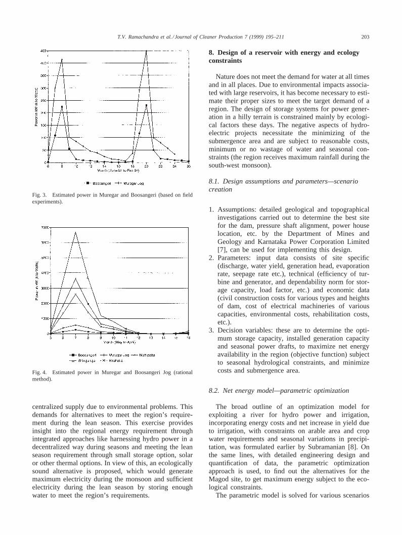
sonal. Power generated during June to September is suf-ficient to meet the energy needs of the nearby villages.Power computed for these streams is shown in Fig. 3.

Stream flow measurement (indirect method)—empiri-cal formula: the runoff (R) and precipitation (P in cm)relationship determined by regression analyses based onour field dataR 5 0.85*P 1 30.5, with r 5 0.89 andthe percentage error is 1.2.

7.4. Rational method

In order to estimate the hydro power potential ofungauged streams, either the rational or empiricalrelationship of runoff and precipitation is used. In therational method, monthly yield is derived by assuming a

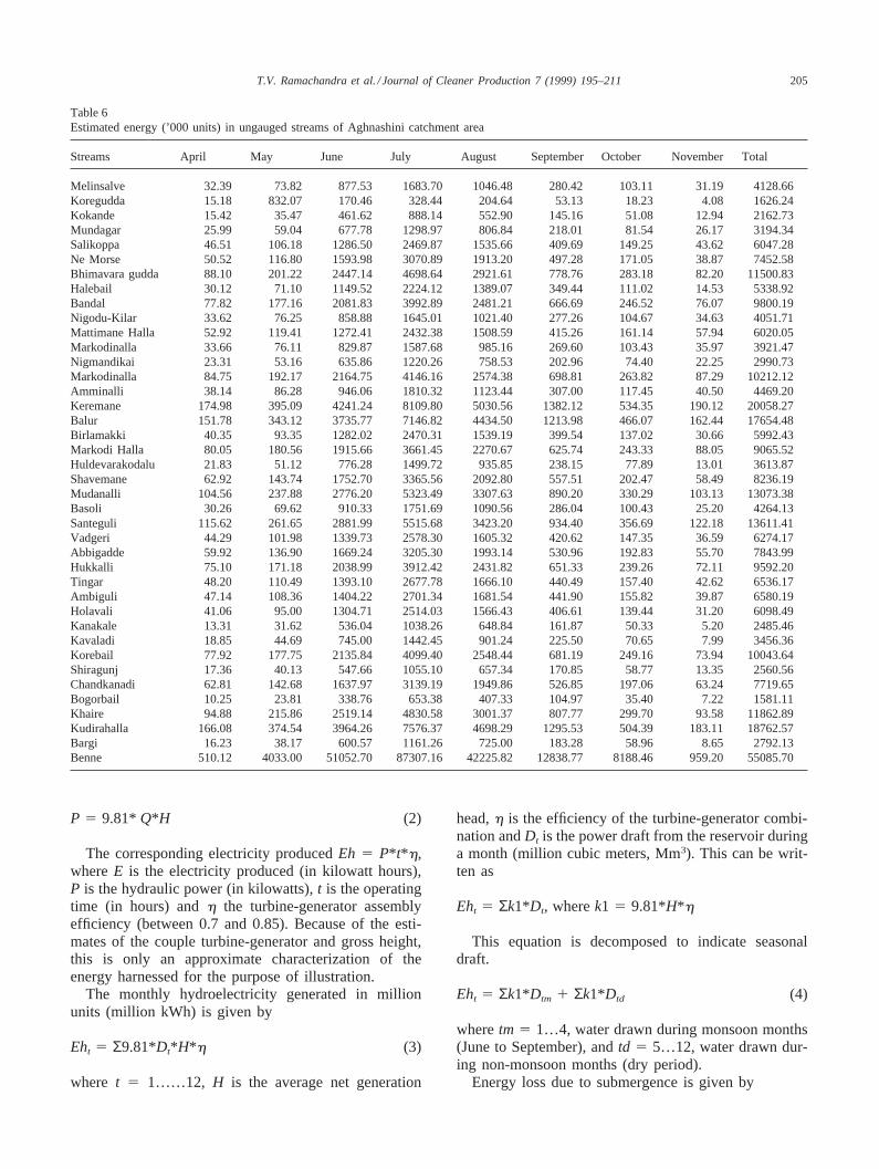
suitable runoff coefficient (which depends on catchmenttype). For each site, Yield (Y 5 C*A*P) is computedwith the knowledge of catchment area (A), catchmentcoefficient (C) and precipitation (P). An attempt hasbeen made to compute the monthly yield from catch-ments by this method, and subsequently the power thatcould be harvested from the streams. Estimated monthlypower by the indirect method is shown pictorially in Fig.4. This corresponds with the power computed by thedirect method (of the gauged streams Boosangeri andMuregar). Hence, we use the rational method to computehydro power of ungauged streams. This study exploresthe possibility of harnessing hydro potential in an eco-logically sound way (by having run-of-river plants withno storage options) to suit the requirements of the region.


Table 4Catchment area, stream slope, catchment slope computed for various streams of Aghnashini river

Feasible sites Latitude Longitude Catchment area Height Stream slope Catchment slope

From To From To

Unchalli 14°209 14°259 74°459 74°509 605.67 360.00 35.54 26.04Benne 14°259 14°329 74°359 74°409 140.75 400.00 23.96 17.87Melinsalve 14°309 14°379 74°359 74°409 20.60 93.75 11.17 12.66Koregudda 14°309 14°359 74°359 74°409 12.62 30.00 11.31 10.08Kokande 14°309 14°359 74°359 74°409 14.60 70.00 17.28 19.57Mundagar 14°309 14°359 74°359 74°409 24.80 60.00 11.31 11.72Salikoppa 14°259 14°309 74°359 74°409 18.90 15.00 36.87 84.29Ne Morse 14°259 14°309 74°389 74°459 12.80 276.50 47.88 50.81Bhimavara 14°259 14°309 74°389 74°459 18.60 290.00 44.03 46.85Halebail 14°259 14°309 74°359 74°409 9.20 280.00 44.03 63.94Bandal 14°309 14°359 74°359 74°409 21.80 210.00 34.99 43.03Nigodu-Kilar 14°209 14°309 74°459 74°559 28.00 67.25 24.81 22.62Keremane 14°209 14°259 74°409 74°459 42.50 218.00 19.97 25.02Balur 14°209 14°259 74°409 74°459 36.80 222.00 27.58 33.38Birlamakki 14°209 14°259 74°409 74°459 12.60 226.00 56.43 61.82Markodi Halla 14°259 14°309 74°409 74°459 48.90 85.50 6.10 20.72Huldevarakodalu 14°229 14°289 74°359 74°409 48.90 85.50 6.10 20.72Huldeva 14°229 14°289 74°359 74°409 10.20 170.00 51.03 58.76Shavemane 14°229 14°289 74°359 74°409 18.40 210.00 43.03 58.76Mudanalli 14°229 14°289 74°359 74°409 22.60 270.00 44.47 49.33Basolli 14°229 14°289 74°359 74°409 14.40 14.00 34.99 30.96Santeguli 14°229 14°289 74°309 74°359 33.20 190.00 26.87 26.46Vadgeri 14°229 14°309 74°409 74°459 14.20 209.00 37.24 44.12Abbigadde 14°229 14°309 74°409 74°459 18.40 200.00 45.00 51.71Hukkalli 14°229 14°309 74°409 74°459 20.40 220.00 48.81 54.18Tingar 14°259 14°309 74°309 74°409 16.20 190.00 32.35 30.02Ambiguli 14°259 14°309 74°309 74°409 14.80 210.00 30.96 37.30Holavali 14°259 14°309 74°309 74°409 12.60 230.00 53.90 61.33Kanakale 14°259 14°309 74°309 74°359 8.60 14.00 48.24 56.19Kavaladi 14°259 14°309 74°309 74°359 8.80 190.00 59.37 58.92Korebail 14°259 14°309 74°309 74°359 19.60 240.00 34.44 35.90Shiragunj 14°259 14°309 74°309 74°359 12.80 95.00 32.35 21.80Chandikanadi 14°259 14°309 74°259 74°329 24.80 145.00 21.14 17.75Bogorbail 14°259 14°309 74°259 74°329 11.60 65.00 27.47 25.64Khaire 14°259 14°309 74°259 74°329 22.60 245.00 31.49 32.35Kudirahalla 14°259 14°359 74°229 74°289 50.44 171.50 19.85 22.15Bargi 14°259 14°359 74°229 74°289 9.60 14.00 44.03 40.18

The Sirsi, Siddapur and Yellapur taluks in hilly terrainamidst evergreen forests with a large number of streamsare ideally suitable for micro, mini or small hydro powerplants. Monthly stream gauging at Muregar and Boosan-geri has revealed that mini hydro power plants could beset up at these sites. The stream at Muregar is perennial,with a flow of about 0.26 m3/s during summer, andpower of the order of 10–20 kW could be generated,while during the monsoon power of 300–400 kW couldbe harnessed.

Computations of discharge by the empirical or rationalmethod, considering precipitation history of the last 100years, and the subsequent power calculated is in con-formity with the power calculations done based onstream gauging. Based on this field experience of gaugedsites, an attempt has been made to compute water inflow(using the indirect method), hydraulic power available,

and energy that could be harnessed monthly for allungauged streams in the Bedthi and Aghnashini rivercatchments. The energy potentials of all streams in thesecatchments are listed in Tables 5 and 6, respectively. Itis estimated that we can generate about 720 and 510million kWh from various streams in the Bedthi andAghnashini catchments.

The potential assessment shows that most of thestreams are seasonal and cater for the needs of localpeople in a decentralized way during the monsoon. Thisensures a continuous power supply during the heavymonsoon, which otherwise gets disrupted due to dislo-cation of electric poles due to heavy winds, and the fall-ing of trees/branches on transmission lines, etc. Adetailed household survey of villages in hilly areasshows that, during the monsoon, people have to spendat least 60 to 65% of the season without electricity from


Fig. 3. Estimated power in Muregar and Boosangeri (based on fieldexperiments).

Fig. 4. Estimated power in Muregar and Boosangeri Jog (rationalmethod).

centralized supply due to environmental problems. Thisdemands for alternatives to meet the region’s require-ment during the lean season. This exercise providesinsight into the regional energy requirement throughintegrated approaches like harnessing hydro power in adecentralized way during seasons and meeting the leanseason requirement through small storage option, solaror other thermal options. In view of this, an ecologicallysound alternative is proposed, which would generatemaximum electricity during the monsoon and sufficientelectricity during the lean season by storing enoughwater to meet the region’s requirements.

8. Design of a reservoir with energy and ecologyconstraints

Nature does not meet the demand for water at all timesand in all places. Due to environmental impacts associa-ted with large reservoirs, it has become necessary to esti-mate their proper sizes to meet the target demand of aregion. The design of storage systems for power gener-ation in a hilly terrain is constrained mainly by ecologi-cal factors these days. The negative aspects of hydro-electric projects necessitate the minimizing of thesubmergence area and are subject to reasonable costs,minimum or no wastage of water and seasonal con-straints (the region receives maximum rainfall during thesouth-west monsoon).

8.1. Design assumptions and parameters—scenariocreation

1. Assumptions: detailed geological and topographicalinvestigations carried out to determine the best sitefor the dam, pressure shaft alignment, power houselocation, etc. by the Department of Mines andGeology and Karnataka Power Corporation Limited[7], can be used for implementing this design.

2. Parameters: input data consists of site specific(discharge, water yield, generation head, evaporationrate, seepage rate etc.), technical (efficiency of tur-bine and generator, and dependability norm for stor-age capacity, load factor, etc.) and economic data(civil construction costs for various types and heightsof dam, cost of electrical machineries of variouscapacities, environmental costs, rehabilitation costs,etc.).

3. Decision variables: these are to determine the opti-mum storage capacity, installed generation capacityand seasonal power drafts, to maximize net energyavailability in the region (objective function) subjectto seasonal hydrological constraints, and minimizecosts and submergence area.

8.2. Net energy model—parametric optimization

The broad outline of an optimization model forexploiting a river for hydro power and irrigation,incorporating energy costs and net increase in yield dueto irrigation, with constraints on arable area and cropwater requirements and seasonal variations in precipi-tation, was formulated earlier by Subramanian [8]. Onthe same lines, with detailed engineering design andquantification of data, the parametric optimizationapproach is used, to find out the alternatives for theMagod site, to get maximum energy subject to the eco-logical constraints.

The parametric model is solved for various scenarios


Table 5Estimated energy (’000 units) in ungauged streams of Bedthi catchment area

Streams April May June July August September October November Total

Arumatti Halla 0.60 5.39 49.69 91.62 52.34 18.86 13.69 4.83 237.02Handinadi 5.73 30.75 230.66 421.41 239.47 91.36 68.28 28.14 1115.80Varangudda 1.40 9.33 77.84 142.92 81.45 30.14 22.18 8.46 373.72Talagudde 14.71 95.64 789.15 1448.24 825.13 306.21 225.68 86.72 3791.48Hirehalla 144.66 784.94 5924.46 10827.26 6153.75 2343.31 1749.60 717.87 28645.85Motigudda 79.52 476.41 3786.89 6937.88 3948.90 1481.03 1097.41 433.60 18241.64Malgaon 5.59 42.09 367.74 676.56 386.02 141.05 103.11 37.94 1760.09Heggarni 32.38 213.18 1768.28 3245.93 1849.60 685.41 504.76 193.21 8492.75Aladbail 11.01 100.24 928.81 1712.91 978.69 352.23 255.43 89.78 4429.09Kotegudda 7.42 94.56 944.56 1746.96 999.78 353.31 253.67 83.94 4484.21Kanchikeri 4.62 56.62 561.39 1038.00 593.95 210.26 151.11 50.31 2666.26Gubbargadda 383.45 1950.83 14172.70 25851.80 14676.60 5654.21 4245.84 1790.20 68725.63Kumbhatt 0.34 45.09 524.11 974.34 559.26 191.15 134.65 39.21 2468.14Datguli 48.43 292.63 2335.73 4280.07 2436.40 912.69 675.87 266.23 11248.05Mulepal 14.15 113.38 1011.34 1862.23 1063.06 386.34 281.63 101.98 4834.11Mogadde Halla 73.69 431.94 3396.50 6219.52 3538.98 1331.43 988.11 393.53 16373.71Garge Halla 40.51 255.78 2083.46 3821.35 2176.46 810.63 598.53 232.24 10018.95Garge Halla 40.51 255.78 2083.46 3821.35 2176.46 810.63 598.53 232.24 10018.95Ramanguli 8.99 66.17 573.32 1054.41 601.48 220.27 161.22 59.71 2745.59Ramanguli 8.99 66.17 573.32 1054.41 601.48 220.27 161.22 59.71 2745.59Barehalla 56.13 329.43 2592.06 4746.61 2700.92 1015.96 753.91 300.12 12495.16Benguli 31.33 234.48 2044.00 3760.12 2145.28 784.36 573.60 211.43 9784.59Benguli 31.33 234.48 2044.00 3760.12 2145.28 784.36 573.60 211.43 9784.59Mulemane 7.72 93.61 926.55 1713.06 980.20 347.14 249.53 83.20 4401.02Matti Gatta 53.26 328.47 2647.09 4852.77 2763.11 1032.25 763.35 298.56 12738.86Hasehalla 184.77 970.35 7187.03 13122.37 7454.11 2854.72 2137.44 888.94 34799.72Vaidyaheggar 3.62 73.37 782.11 1449.85 830.85 289.28 205.96 64.59 3699.64Kaigadi 5.98 85.04 865.36 1601.56 916.93 322.63 231.08 75.31 4103.88Bili Halla 148.90 794.56 5940.22 10850.94 6165.52 2354.53 1760.47 727.29 28742.43Bili Halla 148.90 794.56 5940.22 10850.94 6165.52 2354.53 1760.47 727.29 28742.43Songi Mane 22.88 161.36 1376.14 2529.16 1442.19 530.40 389.07 145.83 6597.03Achave Stream 106.72 583.19 4419.33 8078.13 4591.79 1746.43 1303.18 533.17 21361.93Vatehalla 15.72 89.77 696.69 1274.96 725.20 273.88 203.65 81.89 3361.77Kalalegadde 10.74 62.76 492.76 902.26 513.37 193.23 143.44 57.19 2375.76Pattanadahall 38.07 200.94 1492.58 2725.60 1548.40 592.47 443.41 184.03 7225.50Shalmala 127.19 675.14 5032.03 9190.58 5221.63 1995.92 1493.02 618.15 24353.68Anegundi 14.71 89.62 718.12 1316.13 749.28 280.37 207.51 81.51 3457.24Manigeri 5.38 43.49 388.97 716.31 408.93 148.51 108.22 39.10 1858.90Hosahalli 10.29 67.77 562.20 1032.01 588.06 217.91 160.47 61.42 2700.13Sadashivalli 20.57 123.42 981.76 1798.72 1023.81 383.90 284.43 112.32 4728.95Nilkani 9.98 63.81 522.72 958.99 546.28 203.14 149.87 57.91 2512.69Gunjavati 46.70 245.41 1818.28 3319.95 1885.90 722.17 540.69 224.81 8803.92Tandi Halla 10.95 66.18 528.41 968.28 551.19 206.46 152.89 60.21 2544.57Kaulgi Halla 79.49 424.44 3174.31 5798.58 3294.79 1258.11 940.63 388.50 15358.85Majjige Halla 42.93 222.86 1639.14 2991.76 1699.11 652.10 488.77 204.29 7940.97Mavinkatte 47.65 249.24 1841.73 3362.31 1909.81 731.93 548.22 228.38 8919.27Devigadde 43.81 231.12 1716.38 3134.25 1780.54 681.35 509.95 211.68 8309.09Koppadgadde 17.18 100.37 788.02 1442.89 820.99 309.01 229.38 91.46 3799.29Bajankoppa 12.40 75.78 608.10 1114.58 634.56 237.35 175.62 68.91 2927.30Bharni 11.98 73.70 593.25 1087.52 619.21 231.40 171.14 66.99 2855.19Heggarni 8.32 53.18 435.60 799.16 455.23 169.28 124.89 48.25 2093.91Magod Falls 4695.0 16435.5 161345.0 387522.4 170605.2 60538.7 43563.4 14620.8 859326.1Chandmata 23.34 149.19 1221.85 2241.59 1276.88 474.86 350.34 135.39 5873.46

for optimal utilization of energy in the water and thermalenergy in the region. The objective is to maximize thenet energy available in the region, which is given by

Enet 5 Eh 2 Ebio (1)

This model includes an equation which computesmonthly hydro power production as a function of (a) thevolume of water discharged, (b) the gross head of thiswater, and (c) the efficiency of the couple turbine gener-ator. Hydro power is given by


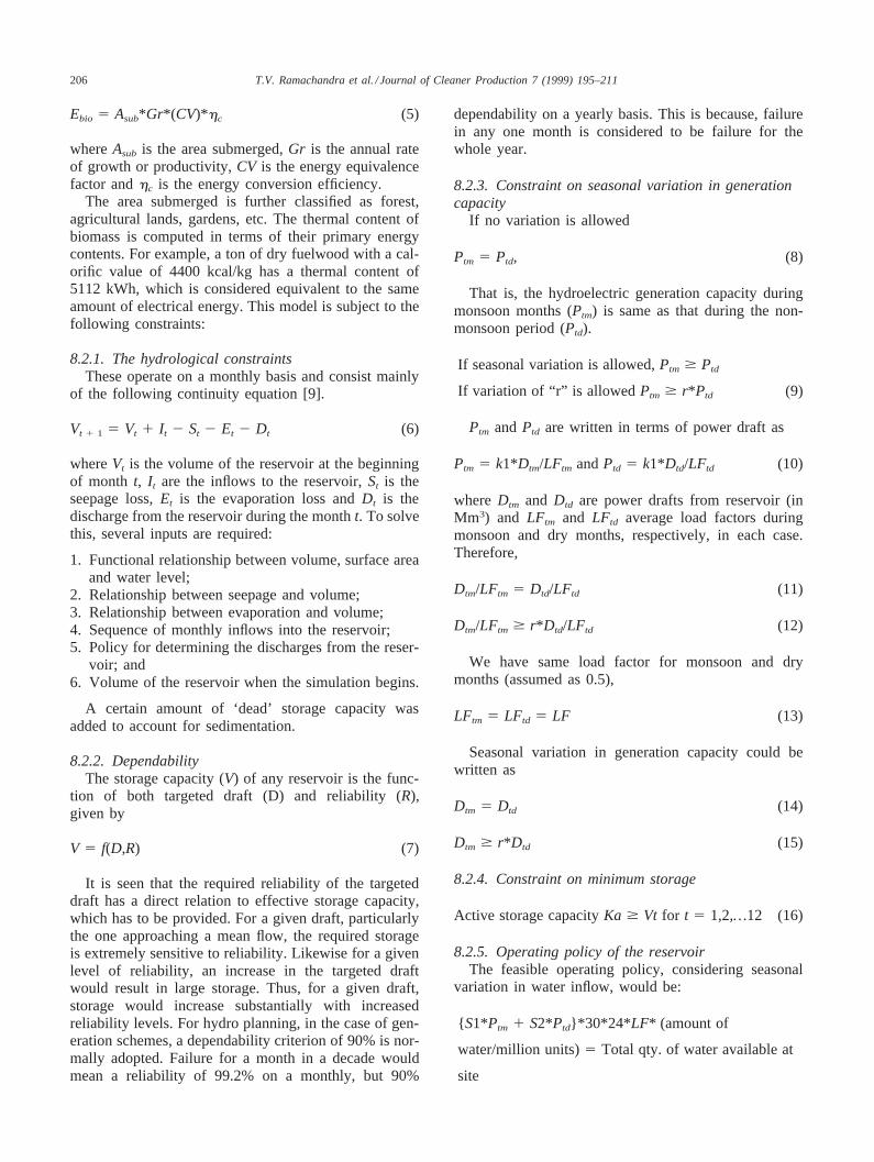
Table 6Estimated energy (’000 units) in ungauged streams of Aghnashini catchment area

Streams April May June July August September October November Total

Melinsalve 32.39 73.82 877.53 1683.70 1046.48 280.42 103.11 31.19 4128.66Koregudda 15.18 832.07 170.46 328.44 204.64 53.13 18.23 4.08 1626.24Kokande 15.42 35.47 461.62 888.14 552.90 145.16 51.08 12.94 2162.73Mundagar 25.99 59.04 677.78 1298.97 806.84 218.01 81.54 26.17 3194.34Salikoppa 46.51 106.18 1286.50 2469.87 1535.66 409.69 149.25 43.62 6047.28Ne Morse 50.52 116.80 1593.98 3070.89 1913.20 497.28 171.05 38.87 7452.58Bhimavara gudda 88.10 201.22 2447.14 4698.64 2921.61 778.76 283.18 82.20 11500.83Halebail 30.12 71.10 1149.52 2224.12 1389.07 349.44 111.02 14.53 5338.92Bandal 77.82 177.16 2081.83 3992.89 2481.21 666.69 246.52 76.07 9800.19Nigodu-Kilar 33.62 76.25 858.88 1645.01 1021.40 277.26 104.67 34.63 4051.71Mattimane Halla 52.92 119.41 1272.41 2432.38 1508.59 415.26 161.14 57.94 6020.05Markodinalla 33.66 76.11 829.87 1587.68 985.16 269.60 103.43 35.97 3921.47Nigmandikai 23.31 53.16 635.86 1220.26 758.53 202.96 74.40 22.25 2990.73Markodinalla 84.75 192.17 2164.75 4146.16 2574.38 698.81 263.82 87.29 10212.12Amminalli 38.14 86.28 946.06 1810.32 1123.44 307.00 117.45 40.50 4469.20Keremane 174.98 395.09 4241.24 8109.80 5030.56 1382.12 534.35 190.12 20058.27Balur 151.78 343.12 3735.77 7146.82 4434.50 1213.98 466.07 162.44 17654.48Birlamakki 40.35 93.35 1282.02 2470.31 1539.19 399.54 137.02 30.66 5992.43Markodi Halla 80.05 180.56 1915.66 3661.45 2270.67 625.74 243.33 88.05 9065.52Huldevarakodalu 21.83 51.12 776.28 1499.72 935.85 238.15 77.89 13.01 3613.87Shavemane 62.92 143.74 1752.70 3365.56 2092.80 557.51 202.47 58.49 8236.19Mudanalli 104.56 237.88 2776.20 5323.49 3307.63 890.20 330.29 103.13 13073.38Basoli 30.26 69.62 910.33 1751.69 1090.56 286.04 100.43 25.20 4264.13Santeguli 115.62 261.65 2881.99 5515.68 3423.20 934.40 356.69 122.18 13611.41Vadgeri 44.29 101.98 1339.73 2578.30 1605.32 420.62 147.35 36.59 6274.17Abbigadde 59.92 136.90 1669.24 3205.30 1993.14 530.96 192.83 55.70 7843.99Hukkalli 75.10 171.18 2038.99 3912.42 2431.82 651.33 239.26 72.11 9592.20Tingar 48.20 110.49 1393.10 2677.78 1666.10 440.49 157.40 42.62 6536.17Ambiguli 47.14 108.36 1404.22 2701.34 1681.54 441.90 155.82 39.87 6580.19Holavali 41.06 95.00 1304.71 2514.03 1566.43 406.61 139.44 31.20 6098.49Kanakale 13.31 31.62 536.04 1038.26 648.84 161.87 50.33 5.20 2485.46Kavaladi 18.85 44.69 745.00 1442.45 901.24 225.50 70.65 7.99 3456.36Korebail 77.92 177.75 2135.84 4099.40 2548.44 681.19 249.16 73.94 10043.64Shiragunj 17.36 40.13 547.66 1055.10 657.34 170.85 58.77 13.35 2560.56Chandkanadi 62.81 142.68 1637.97 3139.19 1949.86 526.85 197.06 63.24 7719.65Bogorbail 10.25 23.81 338.76 653.38 407.33 104.97 35.40 7.22 1581.11Khaire 94.88 215.86 2519.14 4830.58 3001.37 807.77 299.70 93.58 11862.89Kudirahalla 166.08 374.54 3964.26 7576.37 4698.29 1295.53 504.39 183.11 18762.57Bargi 16.23 38.17 600.57 1161.26 725.00 183.28 58.96 8.65 2792.13Benne 510.12 4033.00 51052.70 87307.16 42225.82 12838.77 8188.46 959.20 55085.70

P 5 9.81* Q*H (2)

The corresponding electricity producedEh 5 P* t*h,whereE is the electricity produced (in kilowatt hours),P is the hydraulic power (in kilowatts),t is the operatingtime (in hours) andh the turbine-generator assemblyefficiency (between 0.7 and 0.85). Because of the esti-mates of the couple turbine-generator and gross height,this is only an approximate characterization of theenergy harnessed for the purpose of illustration.

The monthly hydroelectricity generated in millionunits (million kWh) is given by

Eht 5 Σ9.81*Dt*H*h (3)

where t 5 1……12, H is the average net generation

head,h is the efficiency of the turbine-generator combi-nation andDt is the power draft from the reservoir duringa month (million cubic meters, Mm3). This can be writ-ten as

Eht 5 Σk1*Dt, wherek1 5 9.81*H*h

This equation is decomposed to indicate seasonaldraft.

Eht 5 Σk1*Dtm 1 Σk1*Dtd (4)

wheretm 5 1…4, water drawn during monsoon months(June to September), andtd 5 5…12, water drawn dur-ing non-monsoon months (dry period).

Energy loss due to submergence is given by


Ebio 5 Asub*Gr*(CV)*hc (5)

whereAsub is the area submerged,Gr is the annual rateof growth or productivity,CV is the energy equivalencefactor andhc is the energy conversion efficiency.

The area submerged is further classified as forest,agricultural lands, gardens, etc. The thermal content ofbiomass is computed in terms of their primary energycontents. For example, a ton of dry fuelwood with a cal-orific value of 4400 kcal/kg has a thermal content of5112 kWh, which is considered equivalent to the sameamount of electrical energy. This model is subject to thefollowing constraints:

8.2.1. The hydrological constraintsThese operate on a monthly basis and consist mainly

of the following continuity equation [9].

Vt 1 1 5 Vt 1 It 2 St 2 Et 2 Dt (6)

whereVt is the volume of the reservoir at the beginningof month t, It are the inflows to the reservoir,St is theseepage loss,Et is the evaporation loss andDt is thedischarge from the reservoir during the montht. To solvethis, several inputs are required:

1. Functional relationship between volume, surface areaand water level;

2. Relationship between seepage and volume;3. Relationship between evaporation and volume;4. Sequence of monthly inflows into the reservoir;5. Policy for determining the discharges from the reser-

voir; and6. Volume of the reservoir when the simulation begins.

A certain amount of ‘dead’ storage capacity wasadded to account for sedimentation.

8.2.2. DependabilityThe storage capacity (V) of any reservoir is the func-

tion of both targeted draft (D) and reliability (R),given by

V 5 f(D,R) (7)

It is seen that the required reliability of the targeteddraft has a direct relation to effective storage capacity,which has to be provided. For a given draft, particularlythe one approaching a mean flow, the required storageis extremely sensitive to reliability. Likewise for a givenlevel of reliability, an increase in the targeted draftwould result in large storage. Thus, for a given draft,storage would increase substantially with increasedreliability levels. For hydro planning, in the case of gen-eration schemes, a dependability criterion of 90% is nor-mally adopted. Failure for a month in a decade wouldmean a reliability of 99.2% on a monthly, but 90%

dependability on a yearly basis. This is because, failurein any one month is considered to be failure for thewhole year.

8.2.3. Constraint on seasonal variation in generationcapacity

If no variation is allowed

Ptm 5 Ptd, (8)

That is, the hydroelectric generation capacity duringmonsoon months (Ptm) is same as that during the non-monsoon period (Ptd).

If seasonal variation is allowed,Ptm $ Ptd

If variation of “r” is allowedPtm $ r*Ptd (9)

Ptm andPtd are written in terms of power draft as

Ptm 5 k1*Dtm/LFtm andPtd 5 k1*Dtd/LFtd (10)

whereDtm and Dtd are power drafts from reservoir (inMm3) and LFtm and LFtd average load factors duringmonsoon and dry months, respectively, in each case.Therefore,

Dtm/LFtm 5 Dtd/LFtd (11)

Dtm/LFtm $ r*Dtd/LFtd (12)

We have same load factor for monsoon and drymonths (assumed as 0.5),

LFtm 5 LFtd 5 LF (13)

Seasonal variation in generation capacity could bewritten as

Dtm 5 Dtd (14)

Dtm $ r*Dtd (15)

8.2.4. Constraint on minimum storage

Active storage capacityKa $ Vt for t 5 1,2,…12 (16)

8.2.5. Operating policy of the reservoirThe feasible operating policy, considering seasonal

variation in water inflow, would be:

{ S1*Ptm 1 S2*Ptd}*30*24* LF* (amount of

water/million units)5 Total qty. of water available at

site


where S1 5 4, (monsoon season) andS2 5 8, (leanseason) and from Eqs. (10) and (13) this constraintreduces to

4*Dtm 1 8*Dtd 5 Vt 1 1

whereDtm 5 Dtd, if no variation is allowed.Dtm $ r*Dtd where the value of ‘r’ ranges from 1, 2… , andVt+1

5 Vt 1 It 2 St 2 Et 2 Dt.With a change in the dam height, the submergence

area and storage volume changes. The submergence areaand volume computation is discussed later in case stud-ies. The regulation through storage could be shown asfollows:

If Vt 1 It 2 St 2 Et 2 Dt # storage volume of reser-voir (Vs), then

Dt 5 Vt 1 It 2 St 2 Et (17)

If Vt 1 It 2 St 2 Et 2 Dt $ storage volume of reser-voir (Vs), then

Dt 1 d 5 Vt 1 It 2 St 2 Et (18)

whered is the excess quantity available for generation.

8.2.6. Positivity constraintsDecision variables are positive.

Dt $ 0, for all t 5 1,2…12

andVt $ 0, for all t 5 1,2…12

Therefore,Ka $ 0 (19)

This design is implemented for the hydroelectricscheme at Magod.

8.3. River discharge

The hydrology of the Bedthi river was analysed dailyand weekly using 5 years’ daily precipitation data. Theaverage annual yield at Magod is 1125 Mm3 by therational method, compared with 1105 Mm3 by theempirical method. Ninety per cent dependable wateryield is estimated as 995 Mm3. Water yield computedat Magod by the empirical method with 90 years’ pre-cipitation data shows that water quantity varies from0.25 (avg)6 1.25 (SD) during January to 364 (avg)6136 (SD) during July.

8.4. Evaporation, seepage loss and silting capacity

These losses are estimated as 99 Mm3 per annum for100 sq km of the region. About 48% of the basin areais plain with partial vegetation cover receiving moderaterainfall. The remaining area is hilly with evergreen veg-

etation. The silt rate per annum (S) is given by S 5C(A)3/4 whereC 5 4.25 assumed for the basin with plainand forested tracts. For Magod, the silt rate is found tobe 0.83 Mm3 per year. At this siltation rate, the life ofthe reservoir at FRL 450–455 m is about 50 years.

8.5. Dam site

The river Bedthi, flowing in a deep and well definedgorge, drains a total area of 4060 sq km. The site pro-posed is about 0.91 km upstream of the Magod falls, atlongitude 74°459280E and latitude 14°519410N. This sitecommands a basin of 2084 sq km and has an exposedrocky bed at the flanks on either side. The river bed levelhere is 373 m and is 36 m wide. At 450, 460 and 480m contour elevations, the length of the dam would be392, 436 and 579 m, respectively.

8.6. Dam height and submergence area

A dam at this site submerges areas having biomasslike firewood, twigs etc. and bio residues of agriculturaland horticultural lands, which is used for domestic, com-mercial and other purposes. This energy is significant.When the water head is very high and the reservoir pro-file a deep valley with steep walls at its sides can hydro-electric energy be very competitive compared to bioenergy. When the water head is not much and the terrainhas a slope less than 25°, then the smaller depths of areservoir with less submergence area make firewood anattractive option.

In order to find the contours of submergence areascorresponding to certain dam heights, Survey of India’s1:50 000 scale toposheets are used. The area is computedusing a planimeter. The volume of water stored for aparticular dam height computed by assuming the volumebetween two consecutive contours to be trapezoidal is

V12 5 (a1 1 a2)*0.5*h12 (20)

whereV12 is the volume between contours 1 and 2,a1

is the area of spread of contour 1,a2 is the area of spreadof contour 2 andh12 is the height difference betweencontours 1 and 2. The generalized form could be writ-ten as,

Vij = Ok = j − 1

k = i

Vk,k + 1 and i = 1, j = i = 1, i + 2,……,

(21)

The submergence area and corresponding volumecomputed for different dam heights at Magod aredepicted in Fig. 5. This shows that, when the dam heightis 67 m, the submergence area is 5.7 sq km and the vol-


Fig. 5. Dam height and corresponding submergence area.

ume is 106.35 Mm3. Beyond 87 m, there is a steepincrease in submergence area, as is evident from a sub-mergence area of 95.02 sq km for a dam height of 107m. The relationship between the submergence area andthe height of the dam is found to be either powerlaw orexponential (Asub 5 0.38*e(0.048*Hdam)) with r 5 0.99,and percentage error 0.45. Similarly, the probablerelationship between the volume of water and the heightof the dam is exponential (Vdam 5 5.03*e(0.054*Hdam))with r 5 0.99 and percentage error 0.22 (Fig. 6).

Fig. 6. Dam height and corresponding storage capacity.

8.7. Net energy analysis

We have computed the hydro power equivalent ateach site before maximizing the net energy function.Energy from water is computed based on parametricoptimization techniques, listed in Table 7. If variation isallowed betweenPtm and Ptd, it reduces the storagecapacity requirements. By allowing thePtm to Ptd ratioto be 3, we notice that the submergence area saved isabout 69.97%. This results in the reduction of the civilcosts of the project. Regression analysis of these vari-ables gives a hyperbolic relationship, given byEn 5733.86 1 [(1566.28)/Area]2 [(6024.64)/(area)(area)],with r 5 0.99 and percentage error of 1.04. We harnessmore hydroelectric energy by drawing the water duringthe monsoon on a run of river basis and store sufficientquantity to meet the non-monsoon requirements. Thissaved area would also help in meeting the bio resourcerequirements of the region. We notice that by allowingvariation in thePtm andPtd ratio, there is an increase inthe electric energy generated. This is because, forsmaller heights of the dam, the submergence area is lessand therefore evaporation and seepage losses are alsoless.

8.8. Biomass energy from lands to be submerged

The land use pattern in the area to be submerged forvarious heights of dam shows that the area under naturalforest is the major constituent of the submerged land,consisting of evergreen, semi-evergreen and deciduousforests where the primary production of biomass is esti-mated to range between 6.5, 13.5, 20 and 27.5 t/ha/year[10]. Areca and coconut residues from gardens are in therange of 3–4.5 t/ha/year.

The reduction in submergence area implies areduction in the loss of thermal energy. The net energyis computed taking the thermal value of bioresiduesavailable in the region and indicates that with a decreasein dam height, the net energy available increases. Asindicated in Table 8 at Magod, the net energy increasesfrom 417 (for a dam of 107 m and biomass productivityof 6.5 t/ha/year) to 803 million units (for a dam of 67 m).The efficiency of a hydro power station is the combinedefficiency of turbine, generators etc. It is estimated thatthis efficiency is around 70%. For this scenario, the netenergy function becomes

Enet 5 0.7*Eh 2 Ebio(lost)

Enet 5 Eh9 2 Ebio (22)

To account for only the final amount of electricity, thethermal energy content of source is discounted by theconversion efficiency of a thermal power plant (as 35%).With this


Table 7Power (in mega watts) and energy (in million kWh)

Hydel powerSite Height Sub area Volume P1/P2 P1 P2 Energy

(m) (sq km) (million M3) ratio (MW) (MW) (million kWh)

Magod 107 95.03 1736 1 85 85 74797 63.23 1135 1 90 90 79187 28.59 545 3 158 53 76987 28.59 545 4 138 35 76987 28.59 545 6 200 33 78082 20.77 417 6 204 34 79682 20.77 417 4 180 45 79182 20.77 417 3 163 54 79677 16.27 417 7 (for 2 months) 245 35 771

4 (for 2 months) 14077 16.27 417 6 210 35 82077 16.27 417 4 185 46 81177 16.27 417 3 166 55 81172 12.74 243 10 250 25 806

& 8 20070 9.98 186 16 320 20 824

& 8 16067 5.70 106 32 320 10 824

& 16 160

Table 8Hydro, thermal energy and net energy available from submerged area (million kWh)

Dam height Hydro energy Eh9 , ——Bio energy—— > , ——Net energy—— >Eh 0.7 Eh Ebio 0.35*Ebio

@6.5t/h/year Ebio9 Eh-Ebio Eh9-Ebio9

Magod 107 747 523 330 115 417 40797 761 532 219 77 541 45687 780 546 100 35 680 51182 796 557 73 26 723 53277 811 568 58 20 753 54772 816 572 46 16 771 55670 824 576 36 13 788 56467 824 576 20 7 803 569

Enet 5 Eh9 2 0.35*Ebio (whereEh9 is 0.7*Eh) (23)

The result of this computation, given in Table 8,shows that a variation in the net energy available rangesfrom 407 to 569 million units at Magod.

The domestic fuelwood consumption survey of thisregion reveals that 82 to 90% of the households stilldepend on fuelwood and agro residues to meet the dom-estic cooking and water heating requirements. Theannual fuelwood energy requirements are estimated tobe 312 million units. System efficiency considerations,peak power considerations and socioeconomic consider-ations all rule out the possibility of electricity entirelysubstituting fuelwood as a source of domestic energy.Therefore only a fraction of the wood energy is con-verted into electrical energy, that is equal to the fractionof the purely non-thermal consumption of electric energy

in a total wood and electric energy consumption. A damheight of 107 m at Magod submerges about 95.03 sqkm, of which 88.53 sq km is under evergreen and semi-evergreen forests, rich in biodiversity. This necessitateseco-friendly options, to reduce the submergence ofprime forests.

The model and subsequent quantitative analyses dem-onstrates that much of the land could be saved from sub-mergence if the hydroelectric power generation capacityis adjusted according to seasonal variations in the river’srunoff. The viability of a mixed hydro and biomass gen-eration system is shown in energy terms, which leads toa significant reduction in the total area used for powergeneration. Apart from this, there is scope to generatehydroelectric energy from streams in a decentralizedway.


8.9. Economic analysis

8.9.1. Computation of costs: net loss due to forestsubmersion

Forests play a role not only in the social and economicwellbeing of the society but also in maintaining the eco-logical balance. With the submersion of forests, benefitssuch as (a) fuelwood, (b) timber, (c) grass and otherbiomass material, (d) forest products such as cane, bam-boo, gums, resins, drugs, spices, etc., (e) biodiversity, (f)recreation and (g) environmental benefits, such as soilconservation, recycling of water and the control ofhumidity, etc., are lost. Direct costs of the submergedarea are assessed by considering standing biomass in thearea, which is based on species diversity studies carriedout in sample plots at Sonda, Kallabe, etc. In this compu-tation, the price of forest land is taken as Rs 111 200per hectare.

8.10. Loss due to submersion of agriculture andhorticulture land

The costs involved in the submersion of agriculturelands, areca nut gardens and coconut plantations werebased on the market value of the land in this region. Thevalue of areca nut garden is Rs 890 000 per hectare,while for paddy, it is Rs 99 000 per hectare and coconutplantation is about Rs 218 000 per hectare. The detailsof villages submerged and the number of householdsaffected are obtained from government agencies like theVillage Accountant’s office. The displacement andrehabilitation costs were based on the data from earlierhydroelectric projects.

8.11. Annual charges on capital costs

The capital cost depends on (a) civil construction costs(size and type of dam) and (b) cost of generating unit,which depends on the capacity. The capacity is calcu-lated using a normal load factor of 0.5. The schedule ofrates approved by the government recently has been usedin computing civil and electrical costs. Annual capitalrecovery factor (annuity factor) is calculated for the total

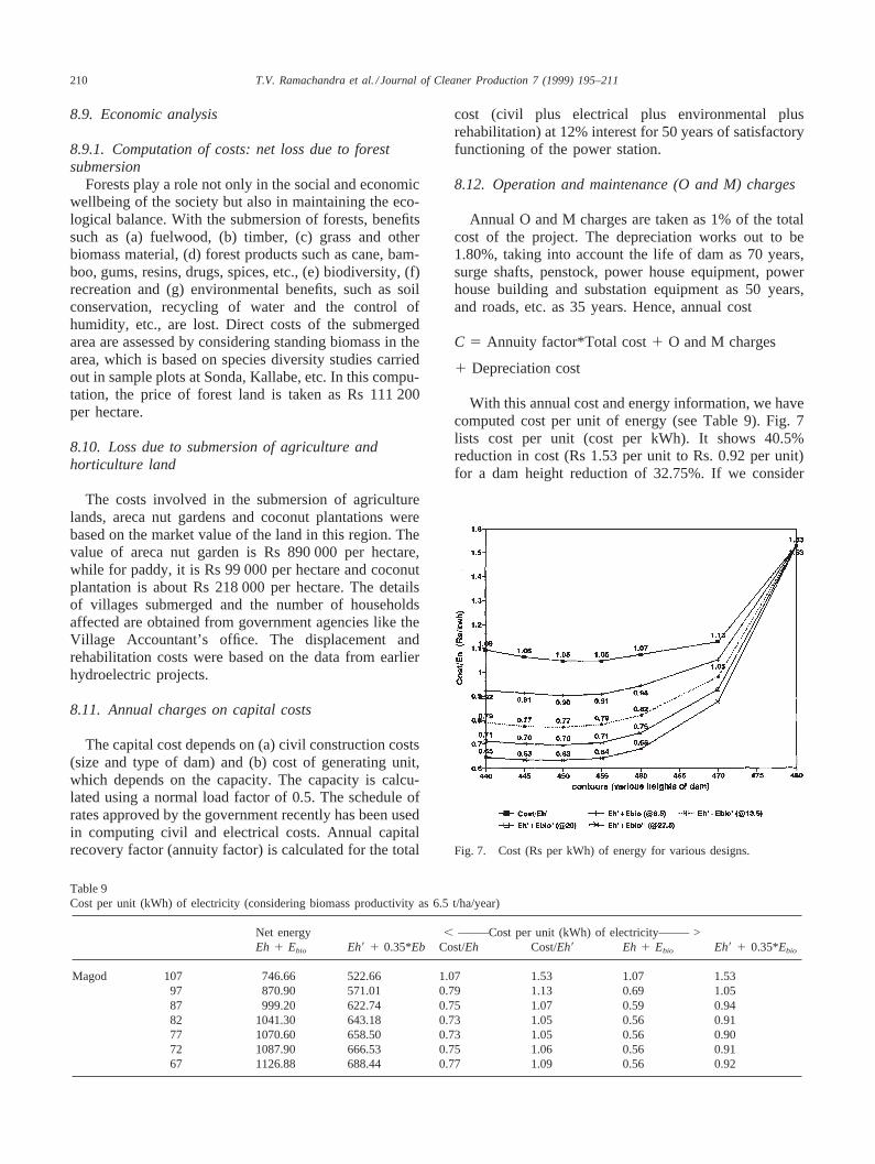
Table 9Cost per unit (kWh) of electricity (considering biomass productivity as 6.5 t/ha/year)

Net energy , ——–Cost per unit (kWh) of electricity——– >Eh 1 Ebio Eh9 1 0.35*Eb Cost/Eh Cost/Eh9 Eh 1 Ebio Eh9 1 0.35*Ebio

Magod 107 746.66 522.66 1.07 1.53 1.07 1.5397 870.90 571.01 0.79 1.13 0.69 1.0587 999.20 622.74 0.75 1.07 0.59 0.9482 1041.30 643.18 0.73 1.05 0.56 0.9177 1070.60 658.50 0.73 1.05 0.56 0.9072 1087.90 666.53 0.75 1.06 0.56 0.9167 1126.88 688.44 0.77 1.09 0.56 0.92

cost (civil plus electrical plus environmental plusrehabilitation) at 12% interest for 50 years of satisfactoryfunctioning of the power station.

8.12. Operation and maintenance (O and M) charges

Annual O and M charges are taken as 1% of the totalcost of the project. The depreciation works out to be1.80%, taking into account the life of dam as 70 years,surge shafts, penstock, power house equipment, powerhouse building and substation equipment as 50 years,and roads, etc. as 35 years. Hence, annual cost

C 5 Annuity factor*Total cost1 O and M charges

1 Depreciation cost

With this annual cost and energy information, we havecomputed cost per unit of energy (see Table 9). Fig. 7lists cost per unit (cost per kWh). It shows 40.5%reduction in cost (Rs 1.53 per unit to Rs. 0.92 per unit)for a dam height reduction of 32.75%. If we consider

Fig. 7. Cost (Rs per kWh) of energy for various designs.


electricity from water resources only, then cost reductionis from Rs 1.53 per unit to Rs 1.09 per unit.

9. Conclusions

The potential assessment of streams in the Bedthi andAghnashini river catchment shows that most of thestreams are seasonal and cater for the needs of localpeople in a decentralized way during the season. Thisensures a continuous power supply during the heavymonsoon, which otherwise gets disrupted due to variousproblems. This study explores the possibility of har-nessing hydro potential in an ecologically sound way tosuit the requirements of the region.

Energy that could be harnessed monthly is computedfor all ungauged streams in the Bedthi and Aghnashiniriver catchments based on the empirical or rationalmethod considering the precipitation history of the last100 years. The hydro energy potentials of streams in theBedthi and Aghnashini river catchments are estimated tobe about 720 and 510 million kWh, respectively.

The net energy analysis explains the upper limit onthe height of a dam and, therefore, the area of the reser-voir for the project to yield a positive net energy. Also,it is noticed that savings in land submergence could beachieved by adjusting hydroelectric generation capacityaccording to seasonal variation in the river runoff. Theparametric optimization technique is used to computeenergy from a hydro source at Magod. By allowing aseasonal generation ratio of 3, the submergence areasaved is about 69.97%, and we notice the subsequentincrease in electric energy generated. This is mainly dueto less evaporation and seepage loss due to a reducedsubmergence area for smaller dam heights.

Net energy analyses carried out by incorporating thebioenergy lost in submergence at Magod show a gain of63.9% for a reduction of 37.3% in dam height. Apartfrom the distinct reduction in submergence area, theoverall reliability of a hydro and thermal combined sys-tem is much higher than that of pure hydro systems(which are very sensitive to fluctuations in rainfall). Thefuelwood requirement in the region is about 312 millionunits (million kWh) for domestic purposes. The netenergy computed for various dam heights indicates thatdams of 67 m height store enough water to meet theregion’s lean season electricity requirements, and thearea saved has a bio resource potential of 319 millionunits, which can cater for the thermal energy demand of312 million units. The cost per unit for various designsof the dam shows a 40.5% reduction in cost (Rs 1.53per unit to Rs 0.92 per unit) for a dam height reductionof 32.75%.

Acknowledgements

This research was supported by grants from the Minis-try of Environment and Forests, the Government of Indiaand Indian Institute of Science. We thank Mr Sampathand Mr Dinesh, Information Analysts, Karnataka StateCouncil for Science and Technology, for taking part inan exploratory survey to identify feasible sites and usefultips in field survey and site identification. We thank ourcolleagues Mr Deepak Shetti, Mr Rosario Furtado, MrKumar and Mr Raghavendra Rao for their assistance inthe collection of stream flow data at regular intervals.

Appendix A

Classification of hydro power plants

Table 10Systems based on power and head: mini, micro and small hydropower plants

Head (metres)Power (kw) Low head Medium High head

Micro up to 50 , 15 15–50 > 50Mini 50–500 , 20 20–100 > 100Small 500–5000 , 25 25–130 > 130

The upper and lower head and output limits adopted for any classi-fication is an indicative only.

References

[1] Raghunath HM. Hydrology: principles, analysis and design. NewDelhi: Wiley Eastern Limited, 1985.

[2] Holland ME. An experimental rainfall–runoff facility. In:Hydrology Papers. Colorado: Colorado State University, 1967.

[3] Markovic RD. Probability functions of best fit to distributions ofannual precipitations and runoff. In: Hydrology Papers. Fort Col-lins, Colorado: Colorado State University, 1976.

[4] Pearson K. Table of incomplete gamma function. Cambridge: TheUniversity Press, 1957.

[5] Zar JH. Biostatistical analysis. Englewood Cliffs, NJ 07632:Prentice Hall, Inc., 1984.

[6] Gordon ND, McMahon TA, Finlayson BL. Stream hydrology: anintroduction for ecologists. England: John Wiley and Sons Ltd,1992.

[7] KPCL. Draft policy paper on implementation of power projectsby KPCL and private sector. Bangalore, India: Karnataka PowerCorporation Ltd, 1993.

[8] Subramanian DK. An optimal energy and water model for designand analysis of water resources of a river with constraints onenergy and ecology. Technical Report No. 8. Bangalore, India:Centre for Ecological Sciences, Indian Institute of Science, 1985.

[9] Maass A, Hufschmidt M, Dorfman R, Thomas HA, Marglin SA,Fair GM. Design of water resources systems—new techniquesfor relating economic objectives, engineering analysis andgovernment planning. Cambridge, Mass.: Harvard UniversityPress, 1962.

[10] Ramachandra TV. Bio energy potential and demand in UttaraKannada district, Karnataka. Special Issue on Bio Energy,IREDA News (India), 1996.

Date post:	27-Apr-2018
Category:	Documents
Upload:	vukien
View:	225 times
Download:	0 times

Hydroelectric resource assessment in Uttara Kannada ... · Journal of Cleaner Production 7 (1999)...

Documents