77
C SQUARED CONSULTING Hydrogen Fueling Station Project Proposal Design Team # 1 May 9, 2011
C SQUARED CONSULTING
Hydrogen Fueling Station Project Proposal
Design Team # 1
May 9, 2011
2
EXECUTIVE SUMMARY
The following report is a detailed engineering proposal for the construction of a hydrogen (H2)
production plant on 2040 8th Ave. in New York City, NY. The purpose of the plant is to convert natural
gas into 99.9999% pure H2 product that will be used as transportation fuel for vehicles.
The main business motivation for this H2 production plant is the growing global market demand for H2
due to interest in using H2 as an alternative transportation fuel. The combination of continuously
increasing fuel demand in the US, declining domestic fossil fuel resource availability and production, and
rising fossil fuel costs are causing the federal and industrial sectors to invest in alternative fuel sources
like H2. Since natural gas is an abundant resource in the US that is significantly cheaper than
conventional fossil fuels, H2 production from natural gas via steam reformation is an attractive fuel
production investment.
The feedstock of the plant is natural gas provided by the Transco pipeline from New Jersey and the
products of the plant that will be sold for revenue are 99.9999% pure H2 and dry ice. For an operating
year of 8000 hours, the plant produces 146,100 kilograms of H2 per year (kg/yr), which is enough to fuel
100 vehicles with a tank size of 4 kg at 700 atmospheres (atm). The plant is designed for a H2 storage
capacity of 24 hours. In addition to H2, the plant also produces 1.5 million kg of dry ice/yr, 48,000 kg of
carbon dioxide (CO2)/yr, and 283,190 gallons of wastewater/yr. The lifetime of the H2 plant is 20 years.
The H2 production technology that is employed in this plant is steam reformation. Steam reformation is
the most established commercial method for H2 production and it is also the cheapest. In this
technique, the natural gas feedstock is reacted with high temperature steam to yield H2. The H2 product
is purified to its 6 nines spec via pressure swing adsorption and the CO2 by-product is separated from
the process stream and converted to dry ice, which is sold for additional revenue to the plant. There are
a total of six major stages in the H2 production process for this plant and they are: pre-treatment, steam
reformation, temperature shift reactions, pressure swing adsorption, CO2 absorption, and dry ice
production.
The working capital for this H2 production plant is $113,600 and the overall capital cost is $2,611,444.
The total fixed operating cost is $742,405 and the total variable operating cost is $349,155. The H2
product will be sold at a retail price of $5/kg, and the dry ice will be sold at $0.05/kg. With a 3% inflation

3
rate, a 35% overall tax rate, and straight-line depreciation, the cumulative cash flow for the plant is a
loss of $28 million by the end of the lifetime of the plant. Adjustments in the costs and product rates for
the H2 plant yield a net profit for the plant by the eleventh year of the plant’s lifetime. At a H2 product
retail rate of $10/kg, a discount rate of 9.82%, and no inflation, the H2 plant reaches its breakeven point
at 11 years and yields a net profit of approximately $4.5 million by the end of the plant lifetime.
Environmental health and safety considerations were incorporated into the design of the H2 production
plant. The plant has zero emissions of hydrogen sulfide (H2S) and carbon monoxide (CO), which are toxic
intermediate products of the production process. CO2, which is a greenhouse gas (GHG), is a by-product
of this production process. Most of the CO2 in the plant’s process stream is recovered and converted to
dry ice and the rest is emitted from the plant at an annual rate of 48,000 kg/yr. Safety precautions were
implemented to avoid risk of explosion or gas leakages. These precautions include putting major
process equipment underground, using double containment for high pressure vessels, adding
temperature and CO detectors to process equipment, and providing intensive safety, process
operations, and materials handling training to production plant employees.
4
TABLE OF CONTENTS
Executive Summary ....................................................................................................................................... 2
Table of Contents .......................................................................................................................................... 4
List of Tables ................................................................................................................................................. 6
List of Figures ................................................................................................................................................ 7
Project Scope ................................................................................................................................................ 8
Process Design Summary .......................................................................................................................... 8
Section I: Natural Gas Processing & Stream Reforming.......................................................................... 13
Zinc Oxide Bed ........................................................................................................................................ 13
Furnace ................................................................................................................................................... 15
Pre-reformer ........................................................................................................................................... 18
Primary steam-methane reformer (SMR) ............................................................................................... 19
Section II: Water Gas Shift ...................................................................................................................... 23
High-temperature shift reactor (HTS) ..................................................................................................... 23
Low-temperature Shift Reactor (LTS) ..................................................................................................... 25
Section III: Flue Gas Treatment ............................................................................................................... 26
MDEA Scrubber ....................................................................................................................................... 26
MDEA Regenerator ................................................................................................................................. 29
Section IV: Dry Ice Production ................................................................................................................ 30
Section V: Product Processing ................................................................................................................ 30
Pressure-swing Adsorber (PSA) ............................................................................................................... 31
Design of Heat Exchangers ...................................................................................................................... 32
Design of Compressors ........................................................................................................................... 36
Design of Pumps ..................................................................................................................................... 36
Design of Tanks ....................................................................................................................................... 37
Heat & Utilities Integration ..................................................................................................................... 39
Cost Analysis ........................................................................................................................................... 42
Separation Unit & Reactor Costs ............................................................................................................ 42
Heat Exchanger Costs.............................................................................................................................. 43
Compressor Costs ................................................................................................................................... 46
Pump Costs ............................................................................................................................................. 47
5
Tank Costs ............................................................................................................................................... 48
Utility Costs ............................................................................................................................................. 49
Plant Lifetime Cost Analysis & Cash Flows .............................................................................................. 52
Capital Costs ............................................................................................................................................ 52
Fixed Operating Costs ............................................................................................................................. 53
Variable Operating Costs ........................................................................................................................ 53
Cash Flow Analysis .................................................................................................................................. 54
Objectives ................................................................................................................................................... 58
Process Design ........................................................................................................................................ 58
Economics ............................................................................................................................................... 58
Environmental & Safety Factors ............................................................................................................. 58
Organization Structure ................................................................................................................................ 60
Operators ................................................................................................................................................ 60
Supervisors & Clerical Assistance ............................................................................................................ 60
Quality Control Plan .................................................................................................................................... 61
Health & Safety Plan ................................................................................................................................... 62
Environmental Health & Safety targets ...................................................................................................... 64
Environmental Targets ............................................................................................................................ 64
Safety Targets ......................................................................................................................................... 65
Project Reporting & Reviews ...................................................................................................................... 67
Supervisor Goals ..................................................................................................................................... 67
Design Team Goals .................................................................................................................................. 67
Construction Team Goals ........................................................................................................................ 67
Production Goals ..................................................................................................................................... 68
Project Enhancement Strategies ................................................................................................................. 69
References .................................................................................................................................................. 70
Appendix A: MATLAB Codes ....................................................................................................................... 71
6
LIST OF TABLES
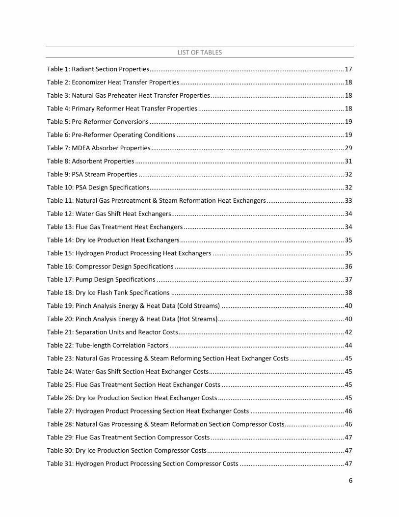
Table 1: Radiant Section Properties ............................................................................................................ 17
Table 2: Economizer Heat Transfer Properties ........................................................................................... 18
Table 3: Natural Gas Preheater Heat Transfer Properties .......................................................................... 18
Table 4: Primary Reformer Heat Transfer Properties ................................................................................. 18
Table 5: Pre-Reformer Conversions ............................................................................................................ 19
Table 6: Pre-Reformer Operating Conditions ............................................................................................. 19
Table 7: MDEA Absorber Properties ........................................................................................................... 29
Table 8: Adsorbent Properties .................................................................................................................... 31
Table 9: PSA Stream Properties .................................................................................................................. 32
Table 10: PSA Design Specifications ............................................................................................................ 32
Table 11: Natural Gas Pretreatment & Steam Reformation Heat Exchangers ........................................... 33
Table 12: Water Gas Shift Heat Exchangers ................................................................................................ 34
Table 13: Flue Gas Treatment Heat Exchangers ......................................................................................... 34
Table 14: Dry Ice Production Heat Exchangers ........................................................................................... 35
Table 15: Hydrogen Product Processing Heat Exchangers ......................................................................... 35
Table 16: Compressor Design Specifications .............................................................................................. 36
Table 17: Pump Design Specifications ........................................................................................................ 37
Table 18: Dry Ice Flash Tank Specifications ................................................................................................ 38
Table 19: Pinch Analysis Energy & Heat Data (Cold Streams) .................................................................... 40
Table 20: Pinch Analysis Energy & Heat Data (Hot Streams) ...................................................................... 40
Table 21: Separation Units and Reactor Costs ............................................................................................ 42
Table 22: Tube-length Correlation Factors ................................................................................................. 44
Table 23: Natural Gas Processing & Steam Reforming Section Heat Exchanger Costs .............................. 45
Table 24: Water Gas Shift Section Heat Exchanger Costs ........................................................................... 45
Table 25: Flue Gas Treatment Section Heat Exchanger Costs .................................................................... 45
Table 26: Dry Ice Production Section Heat Exchanger Costs ...................................................................... 45
Table 27: Hydrogen Product Processing Section Heat Exchanger Costs .................................................... 46
Table 28: Natural Gas Processing & Steam Reformation Section Compressor Costs ................................. 46
Table 29: Flue Gas Treatment Section Compressor Costs .......................................................................... 47
Table 30: Dry Ice Production Section Compressor Costs ............................................................................ 47
Table 31: Hydrogen Product Processing Section Compressor Costs .......................................................... 47
7
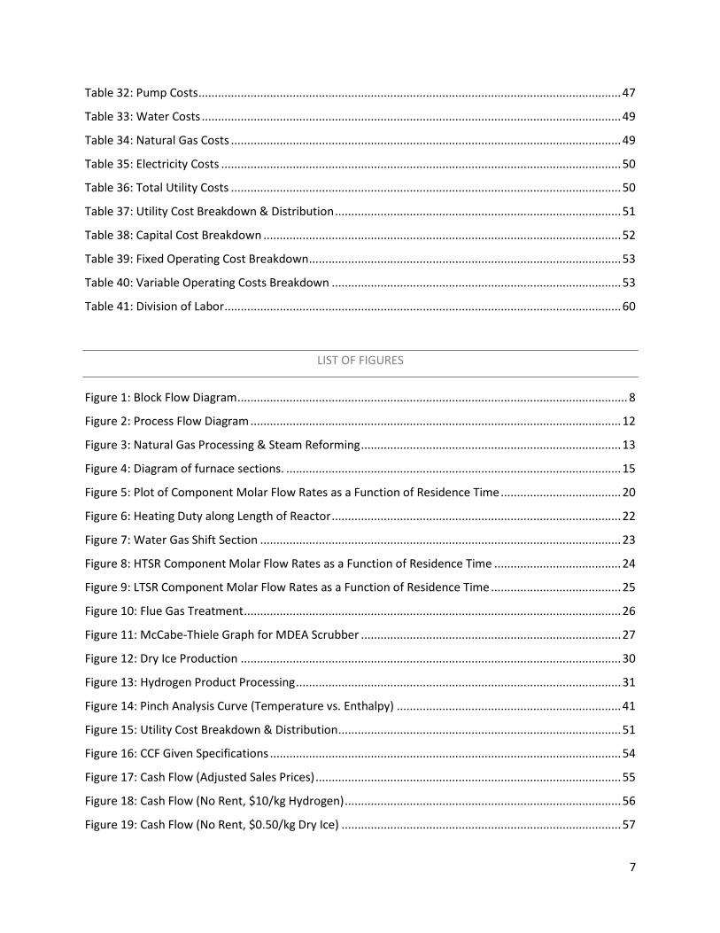
Table 32: Pump Costs .................................................................................................................................. 47
Table 33: Water Costs ................................................................................................................................. 49
Table 34: Natural Gas Costs ........................................................................................................................ 49
Table 35: Electricity Costs ........................................................................................................................... 50
Table 36: Total Utility Costs ........................................................................................................................ 50
Table 37: Utility Cost Breakdown & Distribution ........................................................................................ 51
Table 38: Capital Cost Breakdown .............................................................................................................. 52
Table 39: Fixed Operating Cost Breakdown ................................................................................................ 53
Table 40: Variable Operating Costs Breakdown ......................................................................................... 53
Table 41: Division of Labor .......................................................................................................................... 60
LIST OF FIGURES
Figure 1: Block Flow Diagram ........................................................................................................................ 8
Figure 2: Process Flow Diagram .................................................................................................................. 12
Figure 3: Natural Gas Processing & Steam Reforming ................................................................................ 13
Figure 4: Diagram of furnace sections. ....................................................................................................... 15
Figure 5: Plot of Component Molar Flow Rates as a Function of Residence Time ..................................... 20
Figure 6: Heating Duty along Length of Reactor ......................................................................................... 22
Figure 7: Water Gas Shift Section ............................................................................................................... 23
Figure 8: HTSR Component Molar Flow Rates as a Function of Residence Time ....................................... 24
Figure 9: LTSR Component Molar Flow Rates as a Function of Residence Time ........................................ 25
Figure 10: Flue Gas Treatment .................................................................................................................... 26
Figure 11: McCabe-Thiele Graph for MDEA Scrubber ................................................................................ 27
Figure 12: Dry Ice Production ..................................................................................................................... 30
Figure 13: Hydrogen Product Processing .................................................................................................... 31
Figure 14: Pinch Analysis Curve (Temperature vs. Enthalpy) ..................................................................... 41
Figure 15: Utility Cost Breakdown & Distribution ....................................................................................... 51
Figure 16: CCF Given Specifications ............................................................................................................ 54
Figure 17: Cash Flow (Adjusted Sales Prices) .............................................................................................. 55
Figure 18: Cash Flow (No Rent, $10/kg Hydrogen) ..................................................................................... 56
Figure 19: Cash Flow (No Rent, $0.50/kg Dry Ice) ...................................................................................... 57
8
PROJECT SCOPE
PROCESS DESIGN SUMMARY
The plant was designed to meet all of the requirements specified in the problem description with
minimal energy consumption. In order to balance reliability and efficiency, the design was based on a
traditional steam reforming process, but was scaled down and modified to include carbon capture and
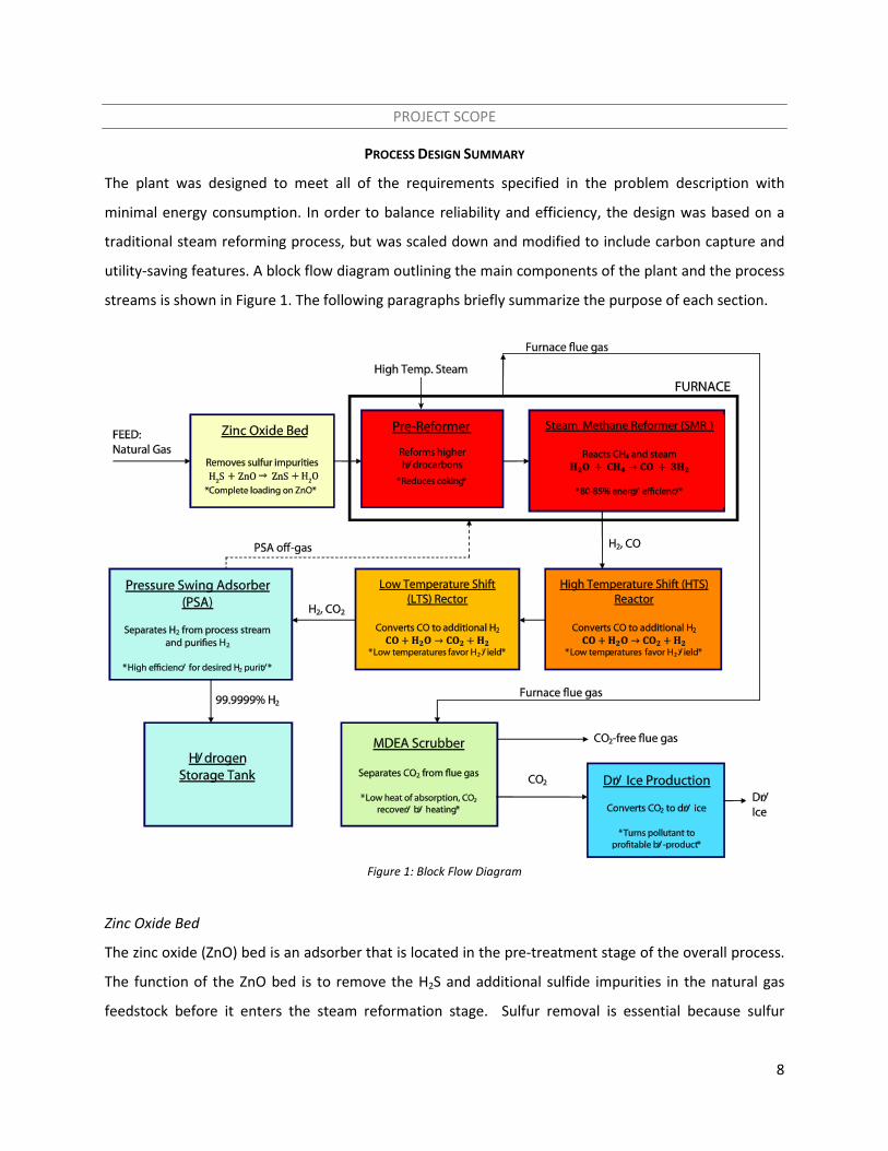
utility-saving features. A block flow diagram outlining the main components of the plant and the process
streams is shown in Figure 1. The following paragraphs briefly summarize the purpose of each section.
Figure 1: Block Flow Diagram
Zinc Oxide Bed
The zinc oxide (ZnO) bed is an adsorber that is located in the pre-treatment stage of the overall process.
The function of the ZnO bed is to remove the H2S and additional sulfide impurities in the natural gas
feedstock before it enters the steam reformation stage. Sulfur removal is essential because sulfur
9
poisons the catalysts in the reactors of this process consequently impairing catalyst performance and
reducing overall production rate. Furthermore, H2S is a poisonous toxic gas therefore it cannot be
emitted from the H2 plant. The feed to the ZnO bed is the natural gas feedstock and the output is a
desulfurized natural gas process stream. ZnO is the adsorbent of choice for desulfurization because it
achieves close to complete loading of H2S.
Furnace
The furnace provides the heat for the reformers, preheats the natural gas and steam, and heats the
contaminated MDEA solution in the flue gas treatment section to regenerate it. The combustion fuel for
the furnace is supplied mostly by the PSA off-gas (~75% by mole) and any remaining required fuel is
supplied by additional natural gas (~25% by mole).
Steam Pre-Reformer
Natural gas contains small amounts of higher hydrocarbons, such as ethane, propane, and butane.
Coking may occur if these hydrocarbons are directly reacted at the high temperatures of the primary
steam-methane reformer; thus it is preferable to let the process stream react in a low-temperature pre-
reformer (operating at 783 K) prior to feeding it to the primary reformer. The pre-reformer converts
approximately 80% of the ethane and essentially all of the propane and butane. A nickel-spinel
(Ni/MgAl2O4) catalyst is used in the pre-reformer, which is the same as that used in the primary
reformer.
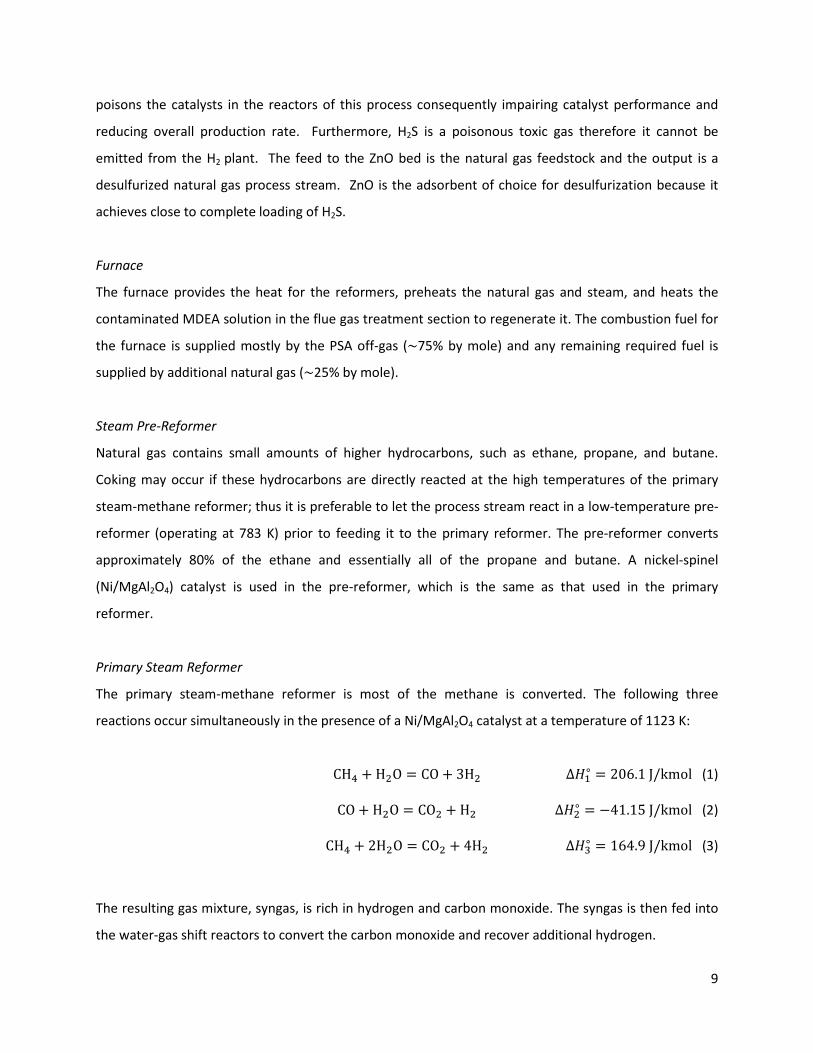
Primary Steam Reformer
The primary steam-methane reformer is most of the methane is converted. The following three
reactions occur simultaneously in the presence of a Ni/MgAl2O4 catalyst at a temperature of 1123 K:
CH4 + H2O = CO + 3H2 Δ𝐻1∘ = 206.1 J/kmol (1)
CO + H2O = CO2 + H2 Δ𝐻2∘ = −41.15 J/kmol (2)
CH4 + 2H2O = CO2 + 4H2 Δ𝐻3∘ = 164.9 J/kmol (3)
The resulting gas mixture, syngas, is rich in hydrogen and carbon monoxide. The syngas is then fed into
the water-gas shift reactors to convert the carbon monoxide and recover additional hydrogen.
10
High-Temperature Shift Reactor
The high-temperature shift reactor is the first of the two water-gas shift reactors. In this reactor,
reaction (2) occurs in the presence of a Fe3O4/Cr2O3 catalyst to convert most of the carbon monoxide to
carbon dioxide and hydrogen at 623 K.
Low-Temperature Shift Reactor
The low-temperature shift reactor is the second of the two water-gas shift reactors. In this reactor,
reaction (2) occurs in the presence of a Cu/ZnO catalyst to convert carbon monoxide to carbon dioxide
and hydrogen at 470 K.
Flue Gas Treatment Section
In order to achieve the goal of zero carbon dioxide emissions, the flue gas must be scrubbed of carbon
dioxide by an absorber. A 50% aqueous MDEA solution was selected as the absorbent, and the absorber
operates at a temperature of 311 K. The cleaned gas exiting the absorber contains only 0.5% carbon
dioxide by mole. The contaminated MDEA solution is regenerated by heating to 443 K, which releases all
of the dissolved carbon dioxide to be sent to the dry ice production section.
MDEA Scrubber
The carbon dioxide separated by the MDEA scrubber is sent to a series of compressors to compress it to
64 atm. The high-pressure carbon dioxide is then flashed to 1 atm, which leads to rapid cooling and the
solidification of most of the carbon dioxide to dry ice. The evaporated portion is recycled into the
compression cycle. This allows the dry ice to be produce without the need of external refrigeration.
Pressure Swing Adsorber (PSA)
The pressure-swing adsorber uses the molecular sieve zeolite 5A to adsorb the impurities of the reactor
effluents. The adsorber uses a two-hour pressure-swing cycle (one hour of adsorption and one hour of
purging) and produces a product stream that is 99.9999% pure in hydrogen. 10% of the high-purity
hydrogen is used to purge the adsorbent, and the released off-gas is then fed into the furnace as fuel.
The hydrogen storage system is designed to store a day’s worth of hydrogen. It consists of a series of
four compression stages to compress the hydrogen to 820 atm. The hydrogen is kept in 24 carbon fiber
tanks that hold the hydrogen for the fueling station.

11
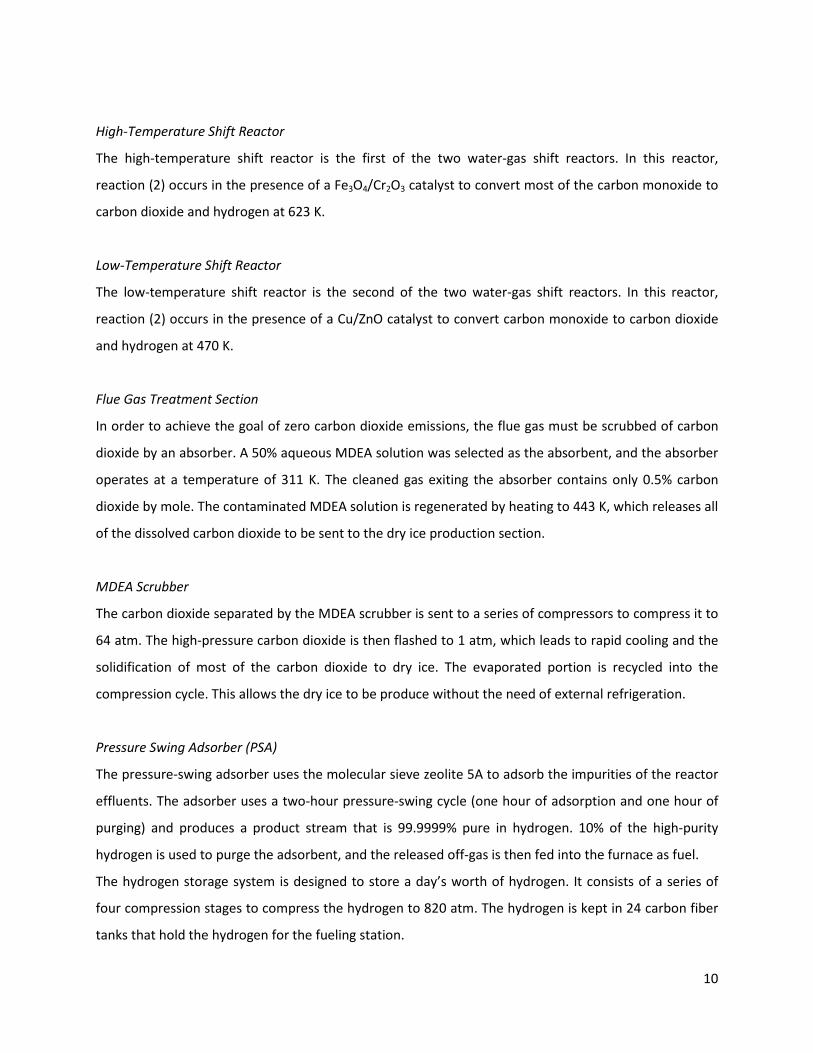
PRO/II Simulation
The process simulation software PRO/II (Invensys, Inc.) was used to model most of the unit operations
and process equipment. A detailed process flow diagram that contains all of the equipment is shown in
Figure 2. The following sections of this report will describe the design methodology used to determine
the specifications of each process unit and present the results.
12
Figure 2: Process Flow Diagram
13
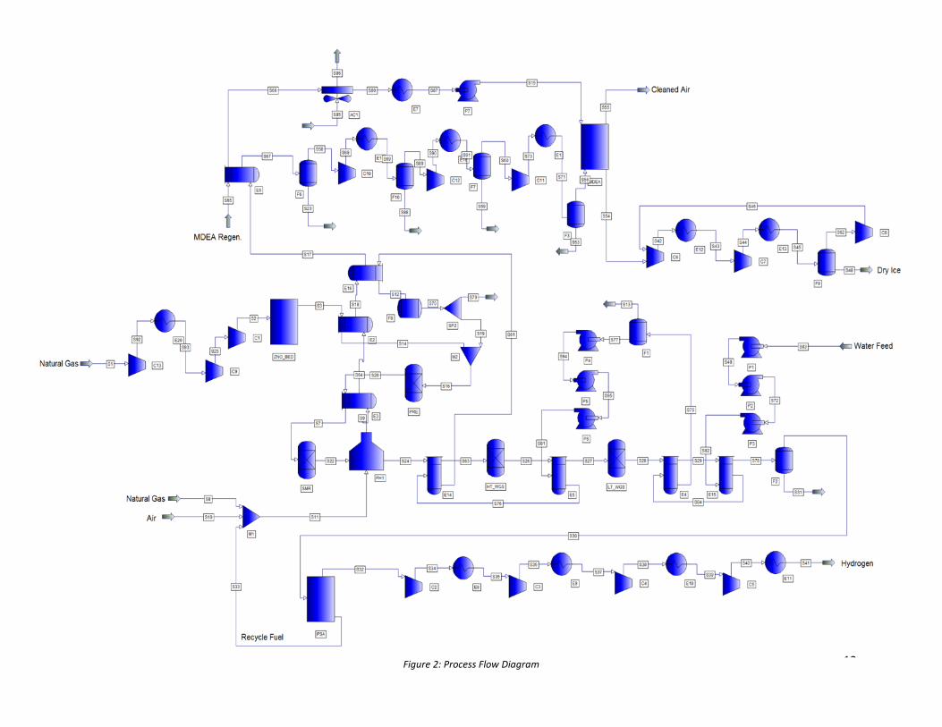
SECTION I: NATURAL GAS PROCESSING & STREAM REFORMING Figure 3 shows the subsection of the process flow diagram that contains the equipment for natural gas
processing and steam reforming. Three compressor stages and one cooler after the first stage were used
to compress the natural gas from atmospheric pressure to a pressure of 30 atm. The design
specifications of all compressors and heat exchangers will be discussed later in the report.
Figure 3: Natural Gas Processing & Steam Reforming
ZINC OXIDE BED
The design factors that determined the size of the ZnO bed for our plant were the amount of natural gas
feedstock, the desulfurization reaction conversion efficiency, and the void fraction. The ZnO bed was
sized based on an annual natural gas feedstock rate of 25,804.8 kmol/yr. This feed rate was determined
previously in the overall mass balances of the H2 production process. Given that the composition of the
natural gas feedstock is 0.122 mol% H2S, the total amount of H2S fed to the ZnO bed is 30.65 kmol/yr.
The amount of ZnO adsorbent required to remove the H2S was determined from the stoichiometry of
the following reaction:
H2S + ZnO → ZnS + H2O
14
This process is essentially irreversible, allowing for complete removal of hydrogen sulfide. Assuming
100% conversion of H2S, the total amount of ZnO required is equivalent to the amount of H2S fed to the
ZnO bed. To determine the mass of ZnO adsorbent required, the molar amount of 30.65 kmol/yr was
multiplied by the molecular weight of ZnO which is 81.38 kg/kmol. The total mass of ZnO adsorbent
required for complete removal of H2S is 2,494.57 kg.
The volume and sizing of the ZnO bed was determined from the volume of adsorbent required and the
void fraction. The volume of adsorbent was calculated by multiplying the mass of adsorbent by the
density of ZnO which is 5606 kg/m3. The required volume of the ZnO adsorbent is 0.445 m3. The overall
volume of the ZnO bed was determined by incorporating the void fraction. Void fraction indicates the
degree of porosity of a packed bed and it is equal to the quotient of the bed bulk density and the density
of a single bed particulate. The bulk density of the ZnO bed is based on the bulk density for BASF©
sulfur removal beds and is equal to 1.15 g/cm3. The density of the ZnO adsorbent particulate is equal to
5.606 g/cm3. The void fraction of the ZnO bed is approximately 0.21 and the overall ZnO bed volume is
0.56 m3. The following sample calculation shows how the void fraction was calculated and
consequently how the overall volume of the ZnO bed was determined:
Bulk Density = 1.15g
cm3
ZnO Particle Density = 5.606g
cm3
Void Fraction =Bulk Density
Particle Density=
1.155.606
= 0.21
Overall ZnO Bed Volume = Volume of ZnO adsorbent
1 − Void Fraction=
0.445 m3
1 − 0.21= 0.56 m3
Overall ZnO Bed Volume = 0.56 m3
The dimensions of the ZnO bed were based on an approximate height to diameter ratio of 2:1. The
height of the ZnO bed was selected to be 1.25 m. Using the volume of the packed bed and the height of
the overall unit, the diameter of the unit was calculated to be 0.76 m. The following sample calculation
shows how the dimensioning of the ZnO bed was determined:
15
𝑉 = 𝜋𝑟2ℎ
𝑉𝑍𝑛𝑂 𝐵𝑒𝑑 = 0.56 m3
ℎ𝑍𝑛𝑂 𝐵𝑒𝑑 = 1.25 m
𝑟 = �𝑉
𝜋 ∗ ℎ= �
0.56 m3
𝜋 ∗ 1.25 m= 0.38 m
𝑑 = 2𝑟 = 2 × 0.38 m = 0.76 m
Dimensions of ZnO bed (ℎ × 𝑑): 1.25 m × 0.76 m
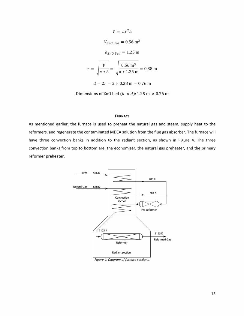
FURNACE
As mentioned earlier, the furnace is used to preheat the natural gas and steam, supply heat to the
reformers, and regenerate the contaminated MDEA solution from the flue gas absorber. The furnace will
have three convection banks in addition to the radiant section, as shown in Figure 4. The three
convection banks from top to bottom are: the economizer, the natural gas preheater, and the primary
reformer preheater.
Figure 4: Diagram of furnace sections.
16
The convection banks1, from top to bottom, are arranged in increasing temperature. The highest
temperature operation in the furnace is the primary reformer, which will be located in the radiant
section of the furnace. The furnace was modeled in PRO/II with the fired heater unit for the radiant
section and a rigorous heat exchanger for each convection bank. The furnace draft is induced by
downstream compressors in the flue gas processing section.
Furnace Radiant Section
Four specifications are required for the fired heater to be fully specified. Since the primary SMR should
be isothermal, the process outlet temperature was set to the primary SMR’s temperature of 1123 K. In
addition to this specification, three assumptions were used:
1. An average tube skin temperature of 1173 K. This temperature provides a temperature
difference of at least 50 K between the process side and the combustion side, but is still in the
operating range of HP-45 steel.2 For this reason, HP-45 was selected as the material for the
radiant tubes as opposed to HK-40.
2. An estimated wall temperature of 1200 K.
3. 1.5% of the firing duty is lost through the wall.
The feed to the fired heater consisted mainly of PSA off-gas, which had a flow rate of 4.27 kmol/hr.
From trial and error, it was determined that an additional 1.15 kmol/hr of natural gas is required to
supply all of the heat for the convection banks and the MDEA regenerator. The air flow rate was
maintained at an excess of 10% above the stoichiometric amount. The radiant heat transfer are was
assumed to be 50% of the total tube area. Using these specifications, the remaining heat transfer
properties for the radiant section were calculated by PRO/II and tabulated in Table 1.
1 The MDEA regenerator was not considered to be a convection bank of the furnace, but as a separate heat
exchanger heated by the flue gas. 2 Behal and Melilli, editors. (1982). Stainless Steel Castings - STP 756. ASTM International.
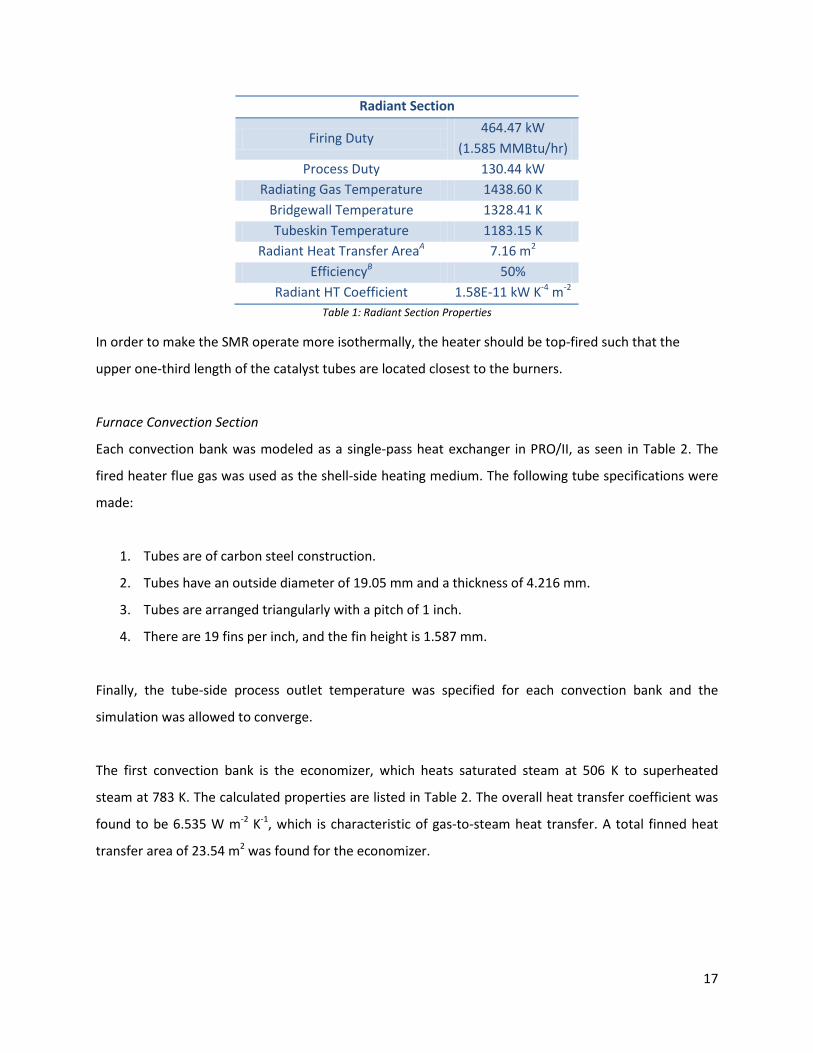
17
Radiant Section
Firing Duty 464.47 kW
(1.585 MMBtu/hr) Process Duty 130.44 kW
Radiating Gas Temperature 1438.60 K Bridgewall Temperature 1328.41 K Tubeskin Temperature 1183.15 K
Radiant Heat Transfer AreaA 7.16 m2 EfficiencyB 50%
Radiant HT Coefficient 1.58E-11 kW K-4 m-2
Table 1: Radiant Section Properties
In order to make the SMR operate more isothermally, the heater should be top-fired such that the
upper one-third length of the catalyst tubes are located closest to the burners.
Furnace Convection Section
Each convection bank was modeled as a single-pass heat exchanger in PRO/II, as seen in Table 2. The
fired heater flue gas was used as the shell-side heating medium. The following tube specifications were
made:
1. Tubes are of carbon steel construction.
2. Tubes have an outside diameter of 19.05 mm and a thickness of 4.216 mm.
3. Tubes are arranged triangularly with a pitch of 1 inch.
4. There are 19 fins per inch, and the fin height is 1.587 mm.
Finally, the tube-side process outlet temperature was specified for each convection bank and the
simulation was allowed to converge.
The first convection bank is the economizer, which heats saturated steam at 506 K to superheated
steam at 783 K. The calculated properties are listed in Table 2. The overall heat transfer coefficient was
found to be 6.535 W m-2 K-1, which is characteristic of gas-to-steam heat transfer. A total finned heat
transfer area of 23.54 m2 was found for the economizer.
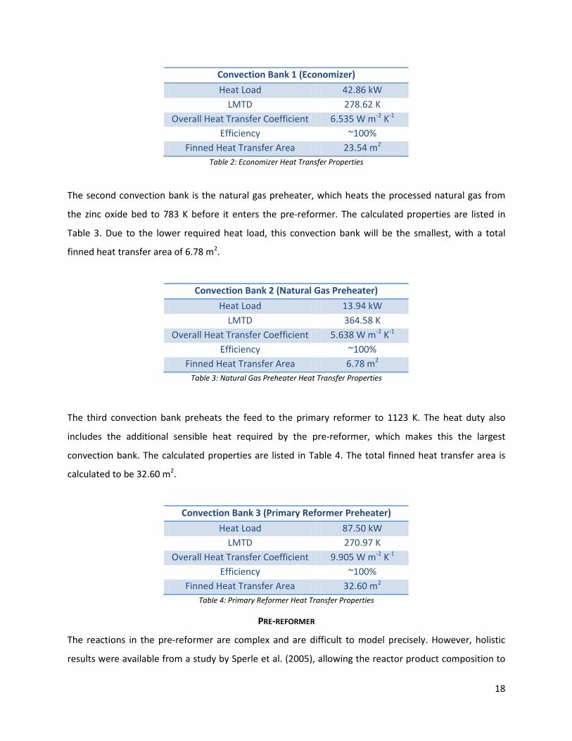
18
Convection Bank 1 (Economizer) Heat Load 42.86 kW
LMTD 278.62 K Overall Heat Transfer Coefficient 6.535 W m-2 K-1
Efficiency ~100% Finned Heat Transfer Area 23.54 m2
Table 2: Economizer Heat Transfer Properties
The second convection bank is the natural gas preheater, which heats the processed natural gas from
the zinc oxide bed to 783 K before it enters the pre-reformer. The calculated properties are listed in
Table 3. Due to the lower required heat load, this convection bank will be the smallest, with a total
finned heat transfer area of 6.78 m2.
Convection Bank 2 (Natural Gas Preheater) Heat Load 13.94 kW
LMTD 364.58 K Overall Heat Transfer Coefficient 5.638 W m-2 K-1
Efficiency ~100% Finned Heat Transfer Area 6.78 m2
Table 3: Natural Gas Preheater Heat Transfer Properties
The third convection bank preheats the feed to the primary reformer to 1123 K. The heat duty also
includes the additional sensible heat required by the pre-reformer, which makes this the largest
convection bank. The calculated properties are listed in Table 4. The total finned heat transfer area is
calculated to be 32.60 m2.
Convection Bank 3 (Primary Reformer Preheater) Heat Load 87.50 kW
LMTD 270.97 K Overall Heat Transfer Coefficient 9.905 W m-2 K-1
Efficiency ~100% Finned Heat Transfer Area 32.60 m2
Table 4: Primary Reformer Heat Transfer Properties
PRE-REFORMER
The reactions in the pre-reformer are complex and are difficult to model precisely. However, holistic
results were available from a study by Sperle et al. (2005), allowing the reactor product composition to
19
be estimated. In their studies, conversions of 3-5% for methane, 80% for ethane, and higher conversions
for higher hydrocarbons were observed.3 To model the pre-reformer, a set of reactions was defined in
PRO/II with the conversions listed in Table 5.
Reaction Conversion
𝐂𝐇𝟒 + 𝐇𝟐𝐎 = 𝐂𝐎 + 𝟑𝐇𝟐 4% 𝐂𝟐𝐇𝟔 + 𝟐𝐇𝟐𝐎 = 𝟐𝐂𝐎 + 𝟓𝐇𝟐 85% 𝐂𝟑𝐇𝟖 + 𝟑𝐇𝟐𝐎 = 𝟑𝐂𝐎 + 𝟕𝐇𝟐 95%
𝐂𝒏𝐇𝒎 + 𝒏𝐇𝟐𝐎 = 𝒏𝐂𝐎 + �𝒏 + 𝒎𝟐�𝐇𝟐;
𝒏 ≥ 𝟒
100%
Table 5: Pre-Reformer Conversions
The reactor was modeled adiabatically, which is similar to the conditions in which it will be operating. A
steam to natural gas ratio of 4 was used to reduce the risk of coking in both the pre-reformer and later
in the primary reformer. The outlet temperature was calculated in PRO/II. The operating conditions are
summarized in Table 6.
Inlet Stream Steam and processed natural gas,
4 to 1 ratio by mole Outlet Stream Pre-reformed gas Temperature 783 K (inlet)
693 K (outlet) Pressure 29 atm
Table 6: Pre-Reformer Operating Conditions
The pre-reformer size is assumed to be equivalent to the heat transfer area required to raise the
temperature of the pre-reformed gas to the primary reformer temperature of 1123 K. This calculation
will be shown in the furnace design description. A more detailed calculation with a kinetic model may be
required to determine if the size of the pre-reformer will be reaction-limited or heat-transfer limited.
PRIMARY STEAM-METHANE REFORMER (SMR)
Xu and Forment’s kinetic equations for steam-methane reforming were used to model the reformer.4 A
reactor model was written in MATLAB5 and used to find the residence time required to achieve a
3 Sperle et al., 2005 4 Xu and Froment, 1989 5 See Listings 1 to 5 in Appendix A for the script and all subroutines used.
20
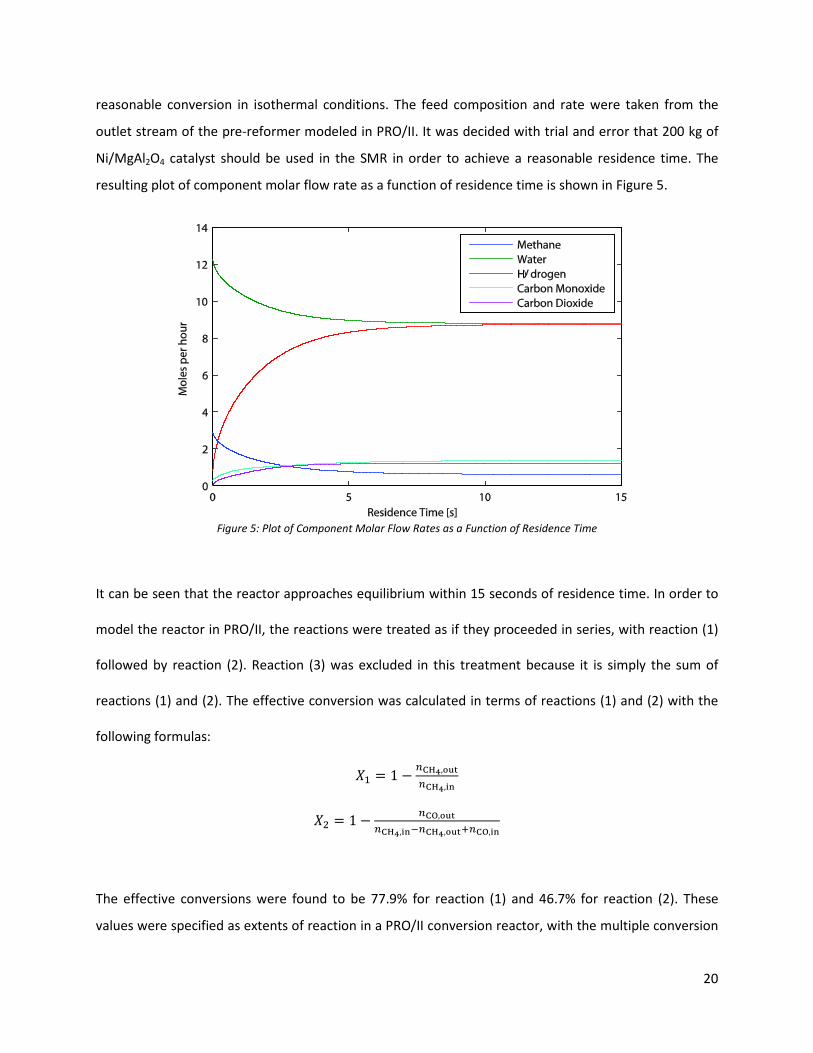
reasonable conversion in isothermal conditions. The feed composition and rate were taken from the
outlet stream of the pre-reformer modeled in PRO/II. It was decided with trial and error that 200 kg of
Ni/MgAl2O4 catalyst should be used in the SMR in order to achieve a reasonable residence time. The
resulting plot of component molar flow rate as a function of residence time is shown in Figure 5.
Figure 5: Plot of Component Molar Flow Rates as a Function of Residence Time
It can be seen that the reactor approaches equilibrium within 15 seconds of residence time. In order to
model the reactor in PRO/II, the reactions were treated as if they proceeded in series, with reaction (1)
followed by reaction (2). Reaction (3) was excluded in this treatment because it is simply the sum of
reactions (1) and (2). The effective conversion was calculated in terms of reactions (1) and (2) with the
following formulas:
𝑋1 = 1 − 𝑛CH4,out
𝑛CH4,in
𝑋2 = 1 − 𝑛CO,out𝑛CH4,in−𝑛CH4,out+𝑛CO,in
The effective conversions were found to be 77.9% for reaction (1) and 46.7% for reaction (2). These
values were specified as extents of reaction in a PRO/II conversion reactor, with the multiple conversion
21
basis set to “reaction.” The PRO/II model produced the same result as that predicted by the MATLAB
model, with 42% hydrogen by mole in the product stream.
The amount of required tubing was calculated based on the residence time, void fraction, and
volumetric flow rate. First, the volume of gas in the reactor was calculated:
𝑉𝑔𝑎𝑠 =�̇�𝜏
𝑉𝑔𝑎𝑠 =�53.6 m3
hr � ∗ �1 hr
3600 s�
15 s
𝑉𝑔𝑎𝑠 = 0.223 m3
Given a void fraction of 𝜀 = 0.528 for Ni/MgAl2O4 catalyst6, the total reactor volume could then be
calculated:
𝑉𝑡𝑜𝑡𝑎𝑙 =𝑉𝑔𝑎𝑠𝜀
𝑉𝑡𝑜𝑡𝑎𝑙 = 0.432 m3
For tubes with an outer diameter of 130 mm and a thickness of 12.5 mm, it was determined that a total
length of 48.8 m would be required.
Length of reactor =𝑉𝑡𝑜𝑡𝑎𝑙
𝜋 �OD − Thickness2 �
2
Length of reactor = 48.8 m
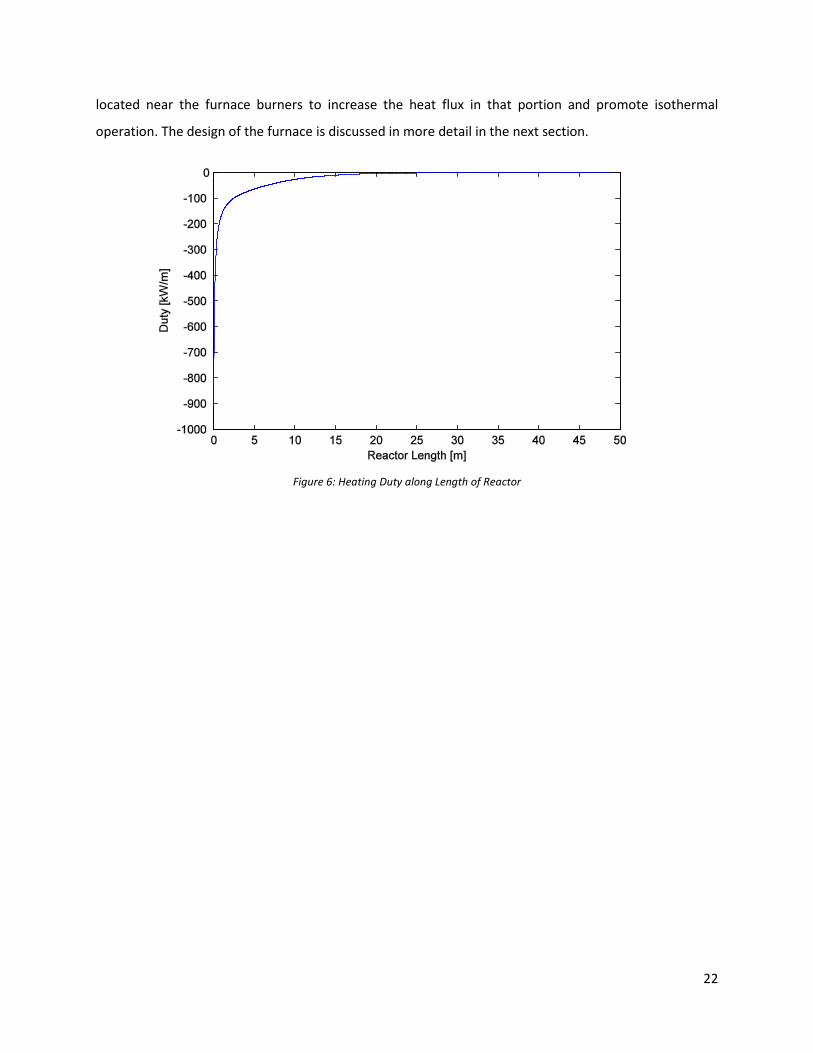
In order to determine the layout of the reformer tubes in the furnace, a plot of heat duty per unit length
along the reactor was generated (see Listing 1 in Appendix A). From Figure 6, it is evident that the most
heat duty is required in the first 10 meters of the reactor. Thus, the entry point of the reactor should be
6 Xu and Froment, 1989
22
located near the furnace burners to increase the heat flux in that portion and promote isothermal
operation. The design of the furnace is discussed in more detail in the next section.
Figure 6: Heating Duty along Length of Reactor
23
SECTION II: WATER GAS SHIFT
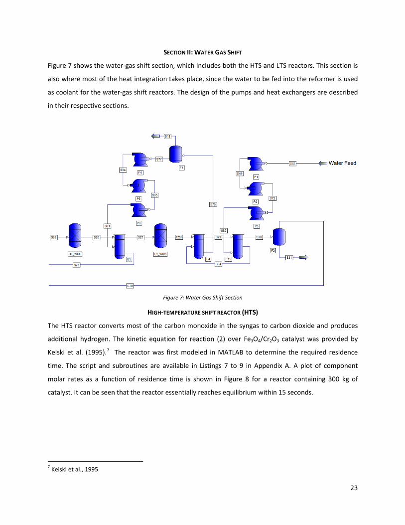
Figure 7 shows the water-gas shift section, which includes both the HTS and LTS reactors. This section is
also where most of the heat integration takes place, since the water to be fed into the reformer is used
as coolant for the water-gas shift reactors. The design of the pumps and heat exchangers are described
in their respective sections.
Figure 7: Water Gas Shift Section
HIGH-TEMPERATURE SHIFT REACTOR (HTS)
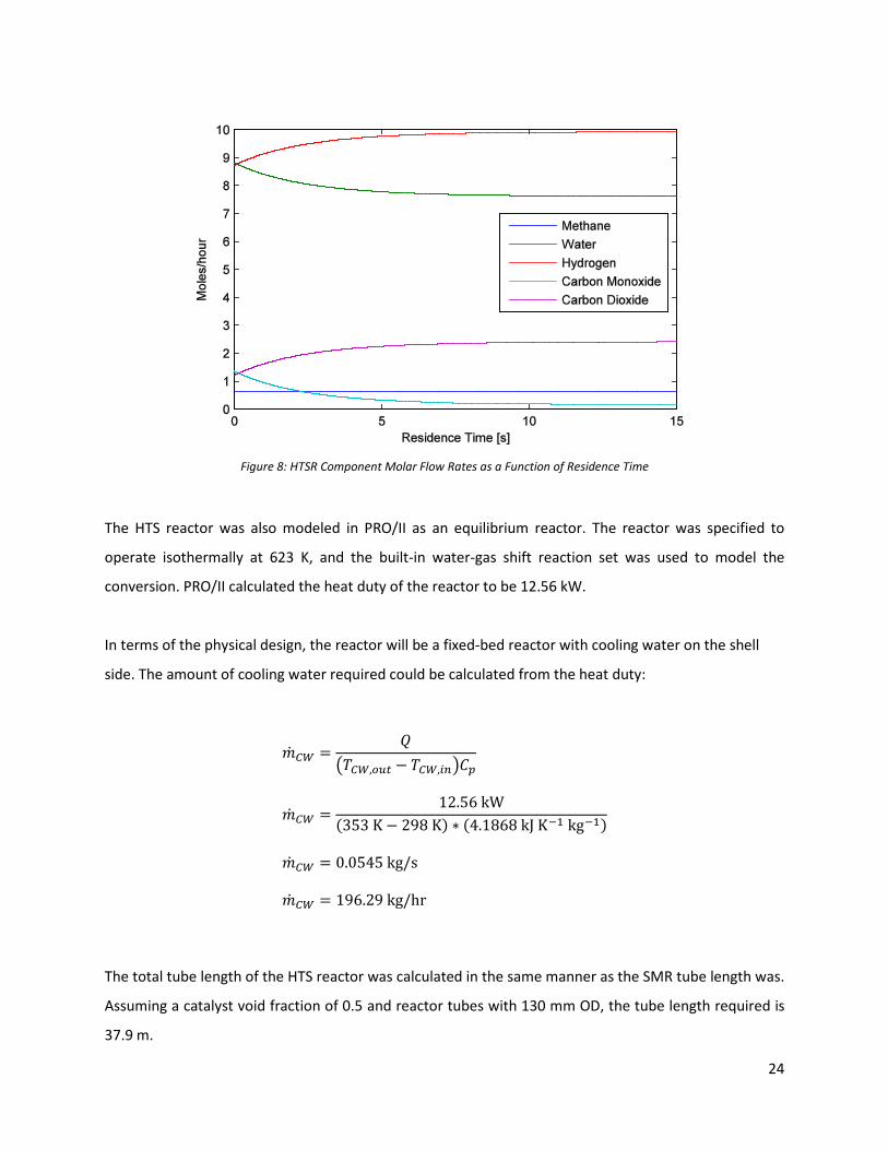
The HTS reactor converts most of the carbon monoxide in the syngas to carbon dioxide and produces
additional hydrogen. The kinetic equation for reaction (2) over Fe3O4/Cr2O3 catalyst was provided by
Keiski et al. (1995).7 The reactor was first modeled in MATLAB to determine the required residence
time. The script and subroutines are available in Listings 7 to 9 in Appendix A. A plot of component
molar rates as a function of residence time is shown in Figure 8 for a reactor containing 300 kg of
catalyst. It can be seen that the reactor essentially reaches equilibrium within 15 seconds.
7 Keiski et al., 1995
24
Figure 8: HTSR Component Molar Flow Rates as a Function of Residence Time
The HTS reactor was also modeled in PRO/II as an equilibrium reactor. The reactor was specified to
operate isothermally at 623 K, and the built-in water-gas shift reaction set was used to model the
conversion. PRO/II calculated the heat duty of the reactor to be 12.56 kW.
In terms of the physical design, the reactor will be a fixed-bed reactor with cooling water on the shell
side. The amount of cooling water required could be calculated from the heat duty:
�̇�𝐶𝑊 =𝑄
�𝑇𝐶𝑊,𝑜𝑢𝑡 − 𝑇𝐶𝑊,𝑖𝑛�𝐶𝑝
�̇�𝐶𝑊 =12.56 kW
(353 K− 298 K) ∗ (4.1868 kJ K−1 kg−1)
�̇�𝐶𝑊 = 0.0545 kg/s
�̇�𝐶𝑊 = 196.29 kg/hr
The total tube length of the HTS reactor was calculated in the same manner as the SMR tube length was.
Assuming a catalyst void fraction of 0.5 and reactor tubes with 130 mm OD, the tube length required is
37.9 m.
25
LOW-TEMPERATURE SHIFT REACTOR (LTS)
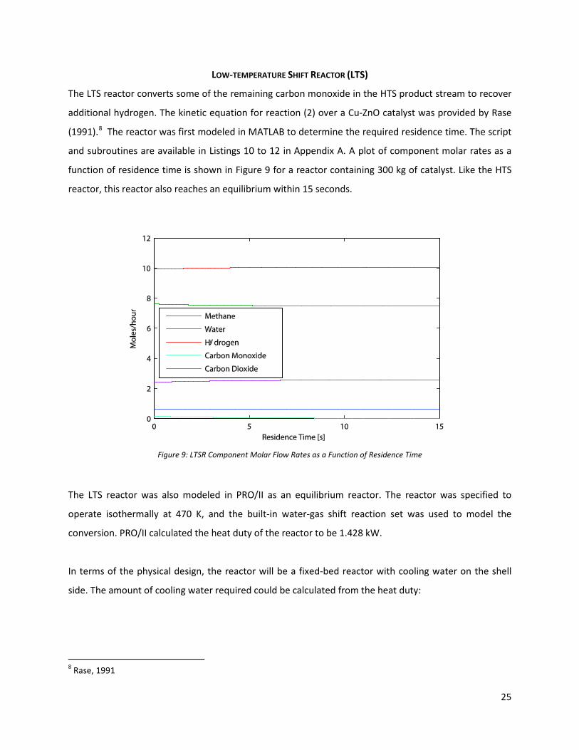
The LTS reactor converts some of the remaining carbon monoxide in the HTS product stream to recover
additional hydrogen. The kinetic equation for reaction (2) over a Cu-ZnO catalyst was provided by Rase
(1991).8 The reactor was first modeled in MATLAB to determine the required residence time. The script
and subroutines are available in Listings 10 to 12 in Appendix A. A plot of component molar rates as a
function of residence time is shown in Figure 9 for a reactor containing 300 kg of catalyst. Like the HTS
reactor, this reactor also reaches an equilibrium within 15 seconds.
Figure 9: LTSR Component Molar Flow Rates as a Function of Residence Time
The LTS reactor was also modeled in PRO/II as an equilibrium reactor. The reactor was specified to
operate isothermally at 470 K, and the built-in water-gas shift reaction set was used to model the
conversion. PRO/II calculated the heat duty of the reactor to be 1.428 kW.
In terms of the physical design, the reactor will be a fixed-bed reactor with cooling water on the shell
side. The amount of cooling water required could be calculated from the heat duty:
8 Rase, 1991
26
�̇�𝐶𝑊 =𝑄
�𝑇𝐶𝑊,𝑜𝑢𝑡 − 𝑇𝐶𝑊,𝑖𝑛�𝐶𝑝
�̇�𝐶𝑊 =1.428 kW
(353 K− 298 K) ∗ (4.1868 kJ K−1 kg−1)
�̇�𝐶𝑊 = 0.00619 kg/s
�̇�𝐶𝑊 = 22.29 kg/hr
The total tube length of the LTS reactor was calculated in the same manner as the SMR and HTS tube
length were. Assuming a catalyst void fraction of 0.5 and reactor tubes with 130 mm OD, the tube length
required is 37.9 m.
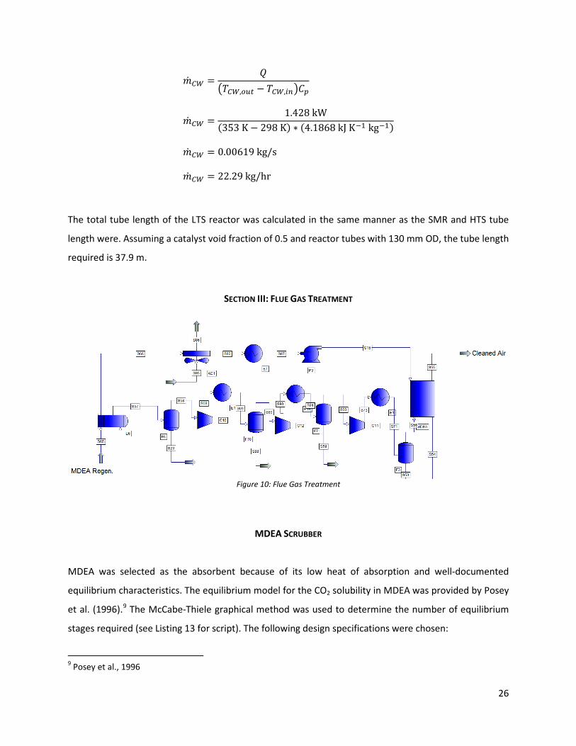
SECTION III: FLUE GAS TREATMENT
Figure 10: Flue Gas Treatment
MDEA SCRUBBER
MDEA was selected as the absorbent because of its low heat of absorption and well-documented
equilibrium characteristics. The equilibrium model for the CO2 solubility in MDEA was provided by Posey
et al. (1996).9 The McCabe-Thiele graphical method was used to determine the number of equilibrium
stages required (see Listing 13 for script). The following design specifications were chosen:
9 Posey et al., 1996
27
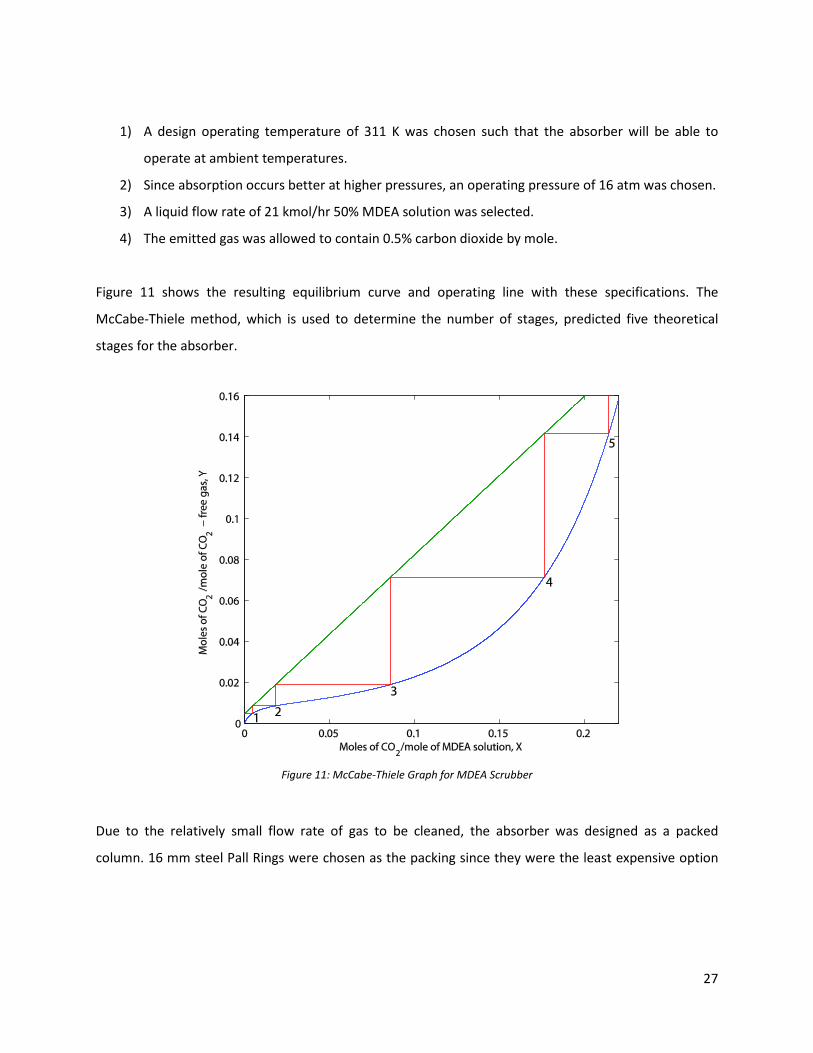
1) A design operating temperature of 311 K was chosen such that the absorber will be able to
operate at ambient temperatures.
2) Since absorption occurs better at higher pressures, an operating pressure of 16 atm was chosen.
3) A liquid flow rate of 21 kmol/hr 50% MDEA solution was selected.
4) The emitted gas was allowed to contain 0.5% carbon dioxide by mole.
Figure 11 shows the resulting equilibrium curve and operating line with these specifications. The
McCabe-Thiele method, which is used to determine the number of stages, predicted five theoretical
stages for the absorber.
Figure 11: McCabe-Thiele Graph for MDEA Scrubber
Due to the relatively small flow rate of gas to be cleaned, the absorber was designed as a packed
column. 16 mm steel Pall Rings were chosen as the packing since they were the least expensive option
28
and only five theoretical stages were required. For Pall Rings, the following correlations were available
to determine the height of a theoretical plate (HETP):10
𝑎𝑝 =5.2𝐷𝑝
=5.2
0.016 𝑚= 325 𝑚2/𝑚3
𝐻𝐸𝑇𝑃 =93𝑎𝑝
=93
325 𝑚2/𝑚3 = 0.286 𝑚
A diameter of 0.2 m was chosen, from which the pressure drop could be estimated. The superficial gas
velocity, 𝑈𝑠, flow parameter, 𝐹𝐿𝑉, were found as follows:
𝑈𝑠 = �𝑉𝑚𝑎𝑠𝑠
𝜌𝑉��𝜋𝐷𝑡2
4 �−1
= �825.732 kg
hr19.175 kg
m3
��𝜋(0.2)2
4 �−1
= 1370.74mhr
= 1.249fts
𝐹𝐿𝑉 = �𝐿𝑚𝑎𝑠𝑠
𝑉𝑚𝑎𝑠𝑠� �𝜌𝑉𝜌𝐿�
= �1440.38825.73
��19.175
1017.49�
= 0.239
The capacity factor, 𝐶𝑝, was then calculated, using a packing factor of 𝐹𝑃 = 78 ft−1 for 16 mm Pall Rings
and the kinematic viscosity of 11.05 centistokes for the MDEA solution.
10 Green and Perry, 2008
29
𝐶𝑝 = 𝑈𝑠 �𝜌𝑉
𝜌𝐿 − 𝜌𝑉�0.5𝐹𝑃0.5𝜈0.5
= �1.249fts
� �19.175
1017.49− 19.175�0.5
(78 ft−1)0.5(11.05 cSt)0.5
= 1.72
From Eckert’s generalized pressure drop correlation11, the pressure drop was found to be approximately
2.5 inches of water per foot of packing height, or 2 kPa per meter of packing. With a packing height of
1.4 m, the pressure drop through the absorber is only 2.9 kPa, or 0.029 atm. The specifications and
calculated properties of the absorber are summarized in Table 7.
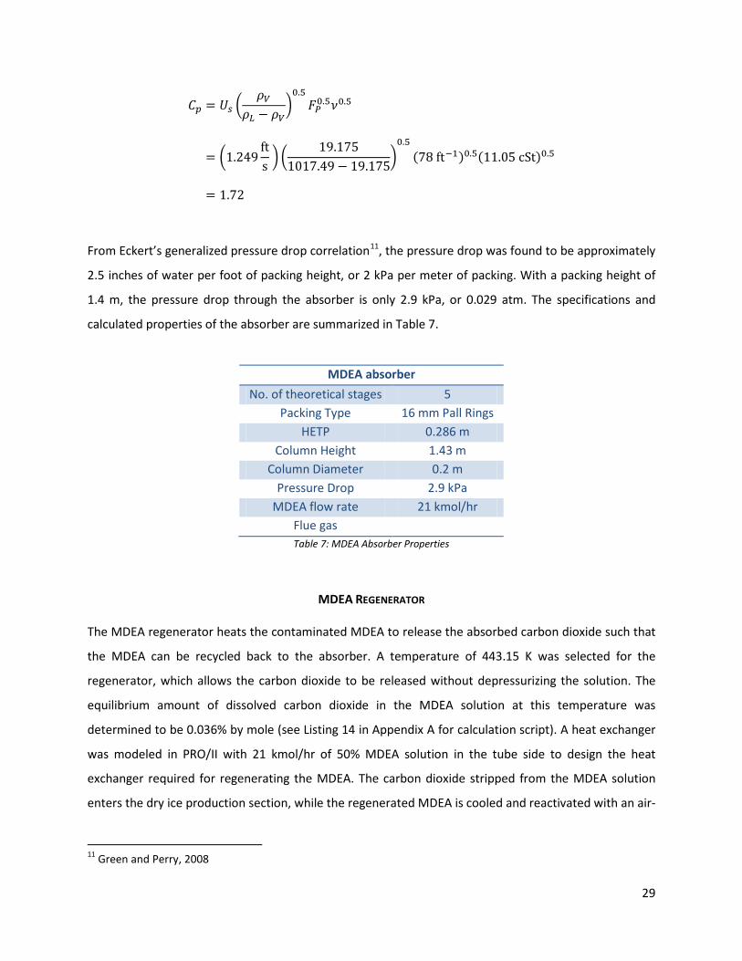
MDEA absorber No. of theoretical stages 5
Packing Type 16 mm Pall Rings HETP 0.286 m
Column Height 1.43 m Column Diameter 0.2 m
Pressure Drop 2.9 kPa MDEA flow rate 21 kmol/hr
Flue gas Table 7: MDEA Absorber Properties
MDEA REGENERATOR The MDEA regenerator heats the contaminated MDEA to release the absorbed carbon dioxide such that
the MDEA can be recycled back to the absorber. A temperature of 443.15 K was selected for the
regenerator, which allows the carbon dioxide to be released without depressurizing the solution. The
equilibrium amount of dissolved carbon dioxide in the MDEA solution at this temperature was
determined to be 0.036% by mole (see Listing 14 in Appendix A for calculation script). A heat exchanger
was modeled in PRO/II with 21 kmol/hr of 50% MDEA solution in the tube side to design the heat
exchanger required for regenerating the MDEA. The carbon dioxide stripped from the MDEA solution
enters the dry ice production section, while the regenerated MDEA is cooled and reactivated with an air-
11 Green and Perry, 2008
30
cooled heat exchanger. The specifications of the heat exchange equipment are available in its respective
section.
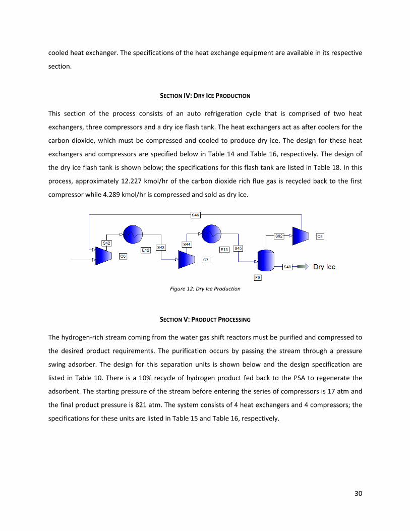
SECTION IV: DRY ICE PRODUCTION This section of the process consists of an auto refrigeration cycle that is comprised of two heat
exchangers, three compressors and a dry ice flash tank. The heat exchangers act as after coolers for the
carbon dioxide, which must be compressed and cooled to produce dry ice. The design for these heat
exchangers and compressors are specified below in Table 14 and Table 16, respectively. The design of
the dry ice flash tank is shown below; the specifications for this flash tank are listed in Table 18. In this
process, approximately 12.227 kmol/hr of the carbon dioxide rich flue gas is recycled back to the first
compressor while 4.289 kmol/hr is compressed and sold as dry ice.
Figure 12: Dry Ice Production
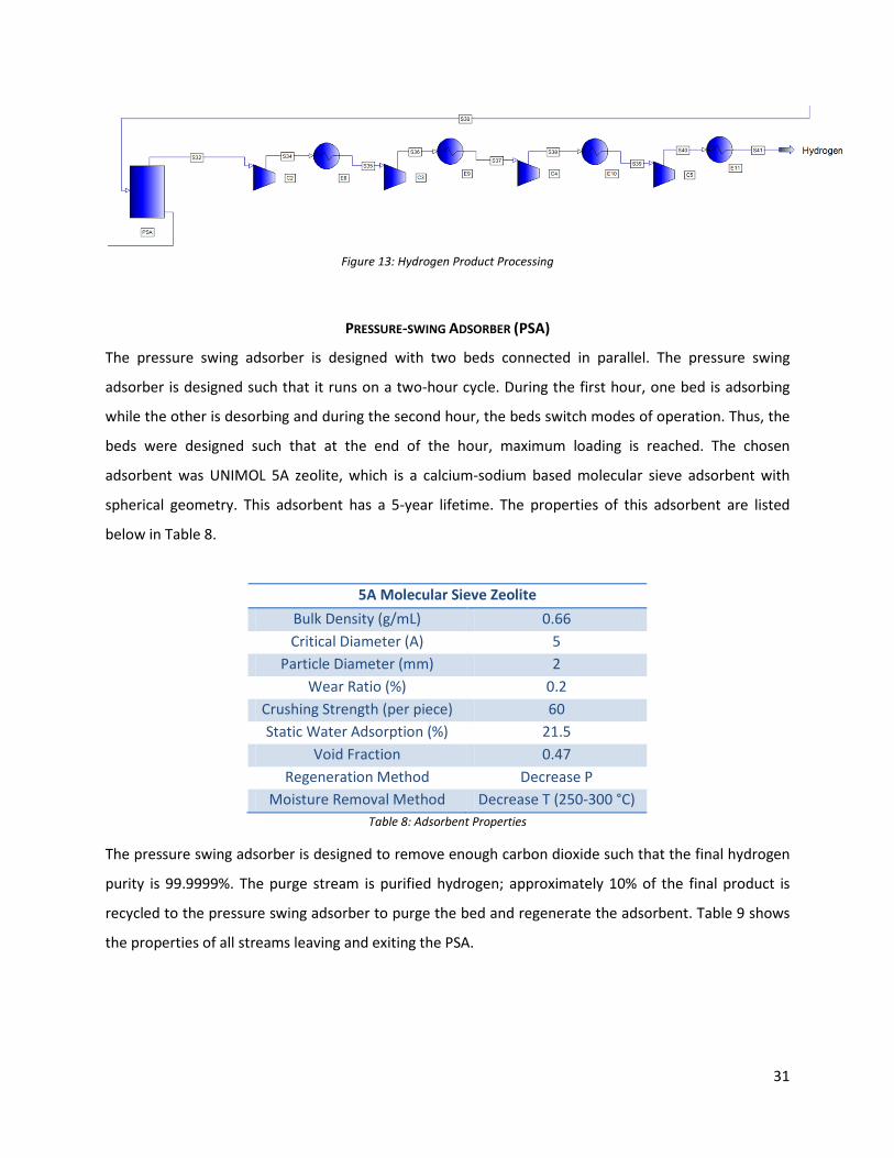
SECTION V: PRODUCT PROCESSING The hydrogen-rich stream coming from the water gas shift reactors must be purified and compressed to
the desired product requirements. The purification occurs by passing the stream through a pressure
swing adsorber. The design for this separation units is shown below and the design specification are
listed in Table 10. There is a 10% recycle of hydrogen product fed back to the PSA to regenerate the
adsorbent. The starting pressure of the stream before entering the series of compressors is 17 atm and
the final product pressure is 821 atm. The system consists of 4 heat exchangers and 4 compressors; the
specifications for these units are listed in Table 15 and Table 16, respectively.
31
Figure 13: Hydrogen Product Processing
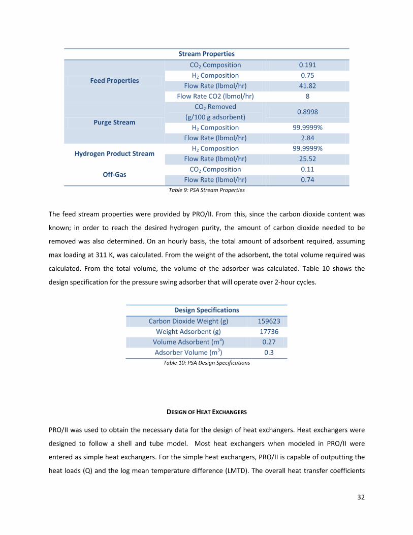
PRESSURE-SWING ADSORBER (PSA)
The pressure swing adsorber is designed with two beds connected in parallel. The pressure swing
adsorber is designed such that it runs on a two-hour cycle. During the first hour, one bed is adsorbing
while the other is desorbing and during the second hour, the beds switch modes of operation. Thus, the
beds were designed such that at the end of the hour, maximum loading is reached. The chosen
adsorbent was UNIMOL 5A zeolite, which is a calcium-sodium based molecular sieve adsorbent with
spherical geometry. This adsorbent has a 5-year lifetime. The properties of this adsorbent are listed
below in Table 8.
5A Molecular Sieve Zeolite Bulk Density (g/mL) 0.66 Critical Diameter (A) 5
Particle Diameter (mm) 2 Wear Ratio (%) 0.2
Crushing Strength (per piece) 60 Static Water Adsorption (%) 21.5
Void Fraction 0.47 Regeneration Method Decrease P
Moisture Removal Method Decrease T (250-300 °C) Table 8: Adsorbent Properties
The pressure swing adsorber is designed to remove enough carbon dioxide such that the final hydrogen
purity is 99.9999%. The purge stream is purified hydrogen; approximately 10% of the final product is
recycled to the pressure swing adsorber to purge the bed and regenerate the adsorbent. Table 9 shows
the properties of all streams leaving and exiting the PSA.
32
Stream Properties
Feed Properties
CO2 Composition 0.191 H2 Composition 0.75
Flow Rate (lbmol/hr) 41.82 Flow Rate CO2 (lbmol/hr) 8
Purge Stream
CO2 Removed (g/100 g adsorbent)
0.8998
H2 Composition 99.9999% Flow Rate (lbmol/hr) 2.84
Hydrogen Product Stream H2 Composition 99.9999%
Flow Rate (lbmol/hr) 25.52
Off-Gas CO2 Composition 0.11
Flow Rate (lbmol/hr) 0.74 Table 9: PSA Stream Properties
The feed stream properties were provided by PRO/II. From this, since the carbon dioxide content was
known; in order to reach the desired hydrogen purity, the amount of carbon dioxide needed to be
removed was also determined. On an hourly basis, the total amount of adsorbent required, assuming
max loading at 311 K, was calculated. From the weight of the adsorbent, the total volume required was
calculated. From the total volume, the volume of the adsorber was calculated. Table 10 shows the
design specification for the pressure swing adsorber that will operate over 2-hour cycles.
Design Specifications Carbon Dioxide Weight (g) 159623
Weight Adsorbent (g) 17736 Volume Adsorbent (m3) 0.27 Adsorber Volume (m3) 0.3
Table 10: PSA Design Specifications
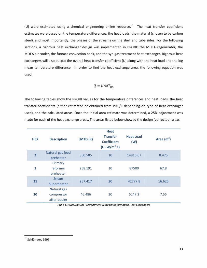
DESIGN OF HEAT EXCHANGERS PRO/II was used to obtain the necessary data for the design of heat exchangers. Heat exchangers were
designed to follow a shell and tube model. Most heat exchangers when modeled in PRO/II were
entered as simple heat exchangers. For the simple heat exchangers, PRO/II is capable of outputting the
heat loads (Q) and the log mean temperature difference (LMTD). The overall heat transfer coefficients
33
(U) were estimated using a chemical engineering online resource.12 The heat transfer coefficient
estimates were based on the temperature differences, the heat loads, the material (chosen to be carbon
steel), and most importantly, the phases of the streams on the shell and tube sides. For the following
sections, a rigorous heat exchanger design was implemented in PRO/II: the MDEA regenerator, the
MDEA air cooler, the furnace convection bank, and the syn-gas treatment heat exchanger. Rigorous heat
exchangers will also output the overall heat transfer coefficient (U) along with the heat load and the log
mean temperature difference. In order to find the heat exchange area, the following equation was
used:
𝑄 = 𝑈𝐴∆𝑇𝑙𝑚
The following tables show the PRO/II values for the temperature differences and heat loads, the heat
transfer coefficients (either estimated or obtained from PRO/II depending on type of heat exchanger
used), and the calculated areas. Once the initial area estimate was determined, a 25% adjustment was
made for each of the heat exchange areas. The areas listed below showed the design (corrected) areas.
HEX Description LMTD (K)
Heat Transfer
Coefficient (U- W/m2 K)
Heat Load (W)
Area (m2)
2 Natural gas feed
preheater 350.585 10 14816.67 8.475
3 Primary
reformer preheater
258.191 10 87500 67.8
21 Steam
Superheater 257.417 20 42777.8 16.625
20 Natural gas compressor after-cooler
46.486 30 5247.2 7.55
Table 11: Natural Gas Pretreatment & Steam Reformation Heat Exchangers
12 Schlünder, 1993
34
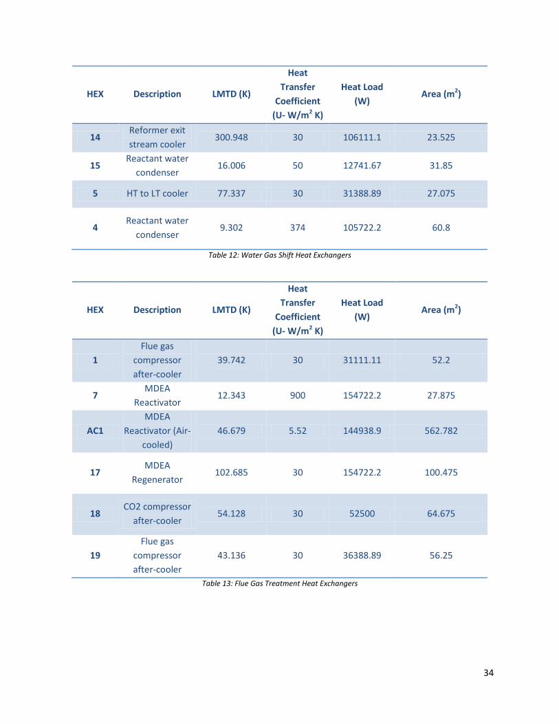
HEX Description LMTD (K)
Heat Transfer
Coefficient (U- W/m2 K)
Heat Load (W)
Area (m2)
14 Reformer exit stream cooler
300.948 30 106111.1 23.525
15 Reactant water
condenser 16.006 50 12741.67 31.85
5 HT to LT cooler 77.337 30 31388.89 27.075
4 Reactant water
condenser 9.302 374 105722.2 60.8
Table 12: Water Gas Shift Heat Exchangers
HEX Description LMTD (K)
Heat Transfer
Coefficient (U- W/m2 K)
Heat Load (W)
Area (m2)
1 Flue gas
compressor after-cooler
39.742 30 31111.11 52.2
7 MDEA
Reactivator 12.343 900 154722.2 27.875
AC1 MDEA
Reactivator (Air-cooled)
46.679 5.52 144938.9 562.782
17 MDEA
Regenerator 102.685 30 154722.2 100.475
18 CO2 compressor
after-cooler 54.128 30 52500 64.675
19 Flue gas
compressor after-cooler
43.136 30 36388.89 56.25
Table 13: Flue Gas Treatment Heat Exchangers
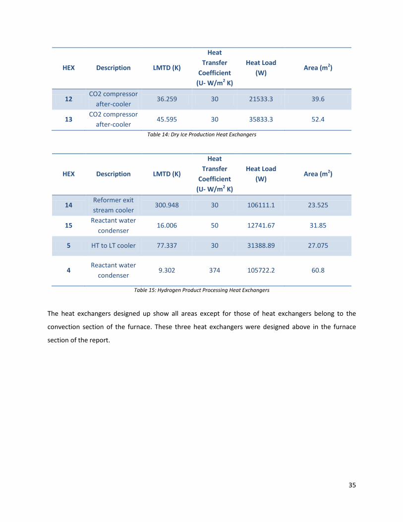
35
HEX Description LMTD (K)
Heat Transfer
Coefficient (U- W/m2 K)
Heat Load (W)
Area (m2)
12 CO2 compressor
after-cooler 36.259 30 21533.3 39.6
13 CO2 compressor
after-cooler 45.595 30 35833.3 52.4
Table 14: Dry Ice Production Heat Exchangers
HEX Description LMTD (K)
Heat Transfer
Coefficient (U- W/m2 K)
Heat Load (W)
Area (m2)
14 Reformer exit stream cooler
300.948 30 106111.1 23.525
15 Reactant water
condenser 16.006 50 12741.67 31.85
5 HT to LT cooler 77.337 30 31388.89 27.075
4 Reactant water
condenser 9.302 374 105722.2 60.8
Table 15: Hydrogen Product Processing Heat Exchangers
The heat exchangers designed up show all areas except for those of heat exchangers belong to the
convection section of the furnace. These three heat exchangers were designed above in the furnace
section of the report.
36
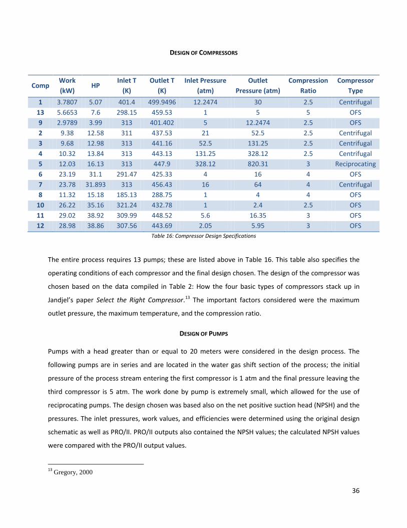
DESIGN OF COMPRESSORS
Comp Work (kW)
HP Inlet T
(K) Outlet T
(K) Inlet Pressure
(atm) Outlet
Pressure (atm) Compression
Ratio Compressor
Type 1 3.7807 5.07 401.4 499.9496 12.2474 30 2.5 Centrifugal
13 5.6653 7.6 298.15 459.53 1 5 5 OFS 9 2.9789 3.99 313 401.402 5 12.2474 2.5 OFS 2 9.38 12.58 311 437.53 21 52.5 2.5 Centrifugal 3 9.68 12.98 313 441.16 52.5 131.25 2.5 Centrifugal 4 10.32 13.84 313 443.13 131.25 328.12 2.5 Centrifugal 5 12.03 16.13 313 447.9 328.12 820.31 3 Reciprocating 6 23.19 31.1 291.47 425.33 4 16 4 OFS 7 23.78 31.893 313 456.43 16 64 4 Centrifugal 8 11.32 15.18 185.13 288.75 1 4 4 OFS
10 26.22 35.16 321.24 432.78 1 2.4 2.5 OFS 11 29.02 38.92 309.99 448.52 5.6 16.35 3 OFS 12 28.98 38.86 307.56 443.69 2.05 5.95 3 OFS
Table 16: Compressor Design Specifications
The entire process requires 13 pumps; these are listed above in Table 16. This table also specifies the
operating conditions of each compressor and the final design chosen. The design of the compressor was
chosen based on the data compiled in Table 2: How the four basic types of compressors stack up in
Jandjel’s paper Select the Right Compressor.13 The important factors considered were the maximum
outlet pressure, the maximum temperature, and the compression ratio.
DESIGN OF PUMPS Pumps with a head greater than or equal to 20 meters were considered in the design process. The
following pumps are in series and are located in the water gas shift section of the process; the initial
pressure of the process stream entering the first compressor is 1 atm and the final pressure leaving the
third compressor is 5 atm. The work done by pump is extremely small, which allowed for the use of
reciprocating pumps. The design chosen was based also on the net positive suction head (NPSH) and the
pressures. The inlet pressures, work values, and efficiencies were determined using the original design
schematic as well as PRO/II. PRO/II outputs also contained the NPSH values; the calculated NPSH values
were compared with the PRO/II output values.
13 Gregory, 2000
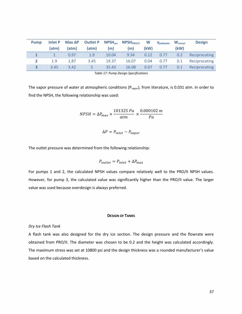
37
Pump Inlet P (atm)
Max ΔP (atm)
Outlet P (atm)
NPSHact (m)
NPSHPRO/II (m)
W (kW)
ηadiabatic Wactual (kW)
Design
1 1 0.97 1.9 10.04 9.34 0.12 0.77 0.2 Reciprocating 2 1.9 1.87 3.45 19.37 16.07 0.04 0.77 0.1 Reciprocating 3 3.45 3.42 5 35.43 16.08 0.07 0.77 0.1 Reciprocating
Table 17: Pump Design Specifications
The vapor pressure of water at atmospheric conditions (Pvapor), from literature, is 0.031 atm. In order to
find the NPSH, the following relationship was used:
𝑁𝑃𝑆𝐻 = ∆𝑃𝑚𝑎𝑥 ×101325 𝑃𝑎
𝑎𝑡𝑚 ×
0.000102 𝑚𝑃𝑎
∆𝑃 = 𝑃𝑖𝑛𝑙𝑒𝑡 − 𝑃𝑣𝑎𝑝𝑜𝑟
The outlet pressure was determined from the following relationship:
𝑃𝑜𝑢𝑡𝑙𝑒𝑡 = 𝑃𝑖𝑛𝑙𝑒𝑡 + ∆𝑃𝑚𝑎𝑥
For pumps 1 and 2, the calculated NPSH values compare relatively well to the PRO/II NPSH values.
However, for pump 3, the calculated value was significantly higher than the PRO/II value. The larger
value was used because overdesign is always preferred.
DESIGN OF TANKS Dry Ice Flash Tank
A flash tank was also designed for the dry ice section. The design pressure and the flowrate were
obtained from PRO/II. The diameter was chosen to be 0.2 and the height was calculated accordingly.
The maximum stress was set at 10800 psi and the design thickness was a rounded manufacturer’s value
based on the calculated thickness.
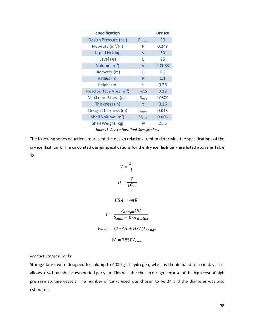
38
Specification Dry Ice Design Pressure (psi) Pdesign 30
Flowrate (m3/hr) F 0.248 Liquid Holdup s 30
Level (%) L 25 Volume (m3) V 0.0083 Diameter (m) D 0.2
Radius (m) R 0.1 Height (m) H 0.26
Head Surface Area (m2) HAS 0.13 Maximum Stress (psi) Smax 10800
Thickness (in) t 0.16 Design Thickness (m) tdesign 0.013
Shell Volume (m3) Vshell 0.003 Shell Weight (kg) W 21.5
Table 18: Dry Ice Flash Tank Specifications
The following series equations represent the design relations used to determine the specifications of the
dry ice flash tank. The calculated design specifications for the dry ice flash tank are listed above in Table
18.
𝑉 =𝑠𝐹𝐿
𝐻 =𝑉𝐷2𝜋
4
𝐻𝑆𝐴 = 4𝜋𝑅2
𝑡 =𝑃𝑑𝑒𝑠𝑖𝑔𝑛(𝑅)
𝑆𝑚𝑎𝑥 − 0.6𝑃𝑑𝑒𝑠𝑖𝑔𝑛
𝑉𝑠ℎ𝑒𝑙𝑙 = (2𝜋𝑅𝐻 + 𝐻𝑆𝐴)𝑡𝑑𝑒𝑠𝑖𝑔𝑛
𝑊 = 7850𝑉𝑠ℎ𝑒𝑙𝑙
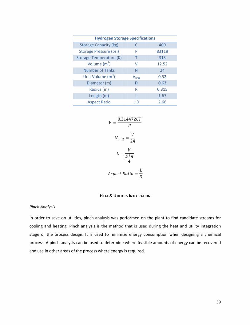
Product Storage Tanks
Storage tanks were designed to hold up to 400 kg of hydrogen, which is the demand for one day. This
allows a 24-hour shut down period per year. This was the chosen design because of the high cost of high
pressure storage vessels. The number of tanks used was chosen to be 24 and the diameter was also
estimated.
39
Hydrogen Storage Specifications
Storage Capacity (kg) C 400 Storage Pressure (psi) P 83118
Storage Temperature (K) T 313 Volume (m3) V 12.52
Number of Tanks N 24 Unit Volume (m3) Vunit 0.52
Diameter (m) D 0.63 Radius (m) R 0.315 Length (m) L 1.67
Aspect Ratio L:D 2.66
𝑉 =8.314472𝐶𝑇
𝑃
𝑉𝑢𝑛𝑖𝑡 =𝑉
24
𝐿 =𝑉𝐷2𝜋
4
𝐴𝑠𝑝𝑒𝑐𝑡 𝑅𝑎𝑡𝑖𝑜 =𝐿𝐷
HEAT & UTILITIES INTEGRATION Pinch Analysis In order to save on utilities, pinch analysis was performed on the plant to find candidate streams for
cooling and heating. Pinch analysis is the method that is used during the heat and utility integration
stage of the process design. It is used to minimize energy consumption when designing a chemical
process. A pinch analysis can be used to determine where feasible amounts of energy can be recovered
and use in other areas of the process where energy is required.
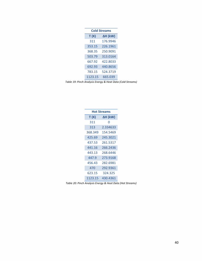
40
Cold Streams
T (K) ΔH (kW) 311 176.9946
353.15 226.1961 368.35 250.9091 503.79 313.0164 667.92 422.8033 692.93 440.8656 783.15 524.3719
1123.15 665.039 Table 19: Pinch Analysis Energy & Heat Data (Cold Streams)
Hot Streams T (K) ΔH (kW) 311 0 313 2.334633
368.349 154.5469 425.69 245.3021 437.53 261.5317 441.16 266.2436 443.13 268.6446 447.9 273.9168
456.43 282.6981 470 292.9361
623.15 324.325 1123.15 430.4361
Table 20: Pinch Analysis Energy & Heat Data (Hot Streams)

41
Figure 14: Pinch Analysis Curve (Temperature vs. Enthalpy)
Energy flow data is obtained as a function of the heat load on a particular stream. The data was
obtained from PRO/II and plotted to form composite hot and cold curves. The hot curves are plotted
from the streams that are releasing heat and the cold curves are plotted from the streams that are
taking in heat. The point at which, the cold and hot streams are closest is called the pinch temperature.
The pinch temperature occurs at the low-temperature water gas shift reactor product stream of 470
Kelvin. From this, heat exchanges can be matched; a hot stream with a temperature above the pinch
point is matched with a cold stream with a temperature below the pinch point. This reduces the heat
exchanger requirements, allows energy to be obtained from within the process, and ultimately, reduced
energy usage and costs. From Figure 14, it is clear that the reactor product streams are good candidates
for heat recovery. This heat was recovered by using it to boil feed water.
42
COST ANALYSIS
The cost analysis included an in-depth study of each component included in the plant. Initial estimates
of equipment and utility costs allowed for further evaluation of the process to minimize utility usage and
equipment sizes. Three different costing protocols were used and compared in order to determine best
estimates for installed equipment costs.
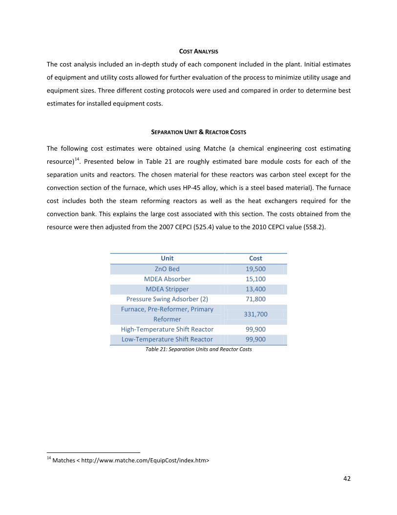
SEPARATION UNIT & REACTOR COSTS
The following cost estimates were obtained using Matche (a chemical engineering cost estimating
resource)14. Presented below in Table 21 are roughly estimated bare module costs for each of the
separation units and reactors. The chosen material for these reactors was carbon steel except for the
convection section of the furnace, which uses HP-45 alloy, which is a steel based material). The furnace
cost includes both the steam reforming reactors as well as the heat exchangers required for the
convection bank. This explains the large cost associated with this section. The costs obtained from the
resource were then adjusted from the 2007 CEPCI (525.4) value to the 2010 CEPCI value (558.2).
Unit Cost ZnO Bed 19,500
MDEA Absorber 15,100 MDEA Stripper 13,400
Pressure Swing Adsorber (2) 71,800 Furnace, Pre-Reformer, Primary
Reformer 331,700
High-Temperature Shift Reactor 99,900 Low-Temperature Shift Reactor 99,900
Table 21: Separation Units and Reactor Costs
14 Matches < http://www.matche.com/EquipCost/index.htm>
43
The highest costs are due to the furnace, steam reforming, and the water-gas shift reactions. This is a
reasonable investment due to the operating temperature and pressures of these components.
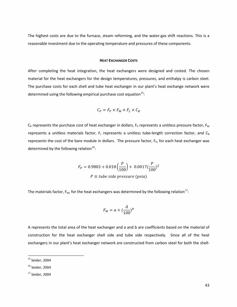
HEAT EXCHANGER COSTS After completing the heat integration, the heat exchangers were designed and costed. The chosen
material for the heat exchangers for the design temperatures, pressures, and enthalpy is carbon steel.
The purchase costs for each shell and tube heat exchanger in our plant’s heat exchange network were
determined using the following empirical purchase cost equation15:
𝐶𝑃 = 𝐹𝑃 × 𝐹𝑀 × 𝐹𝐿 × 𝐶𝐵
CP represents the purchase cost of heat exchanger in dollars, FP represents a unitless pressure factor, FM
represents a unitless materials factor, FL represents a unitless tube-length correction factor, and CB
represents the cost of the bare module in dollars. The pressure factor, FP, for each heat exchanger was
determined by the following relation16:
𝐹𝑃 = 0.9803 + 0.018 �𝑃
100� + 0.0017(
𝑃100
)2
𝑃 ≡ 𝑡𝑢𝑏𝑒 𝑠𝑖𝑑𝑒 𝑝𝑟𝑒𝑠𝑠𝑢𝑟𝑒 (𝑝𝑠𝑖𝑎)
The materials factor, FM, for the heat exchangers was determined by the following relation17:
𝐹𝑀 = 𝑎 + (𝐴
100)𝑏
A represents the total area of the heat exchanger and a and b are coefficients based on the material of
construction for the heat exchanger shell side and tube side respectively. Since all of the heat
exchangers in our plant’s heat exchanger network are constructed from carbon steel for both the shell-
15 Seider, 2004 16 Seider, 2004 17 Seider, 2004
44
side and tube-side, the coefficients a and b are both equal to 0. Therefore, FM for all heat exchangers in
our heat exchanger network is equal to 1.
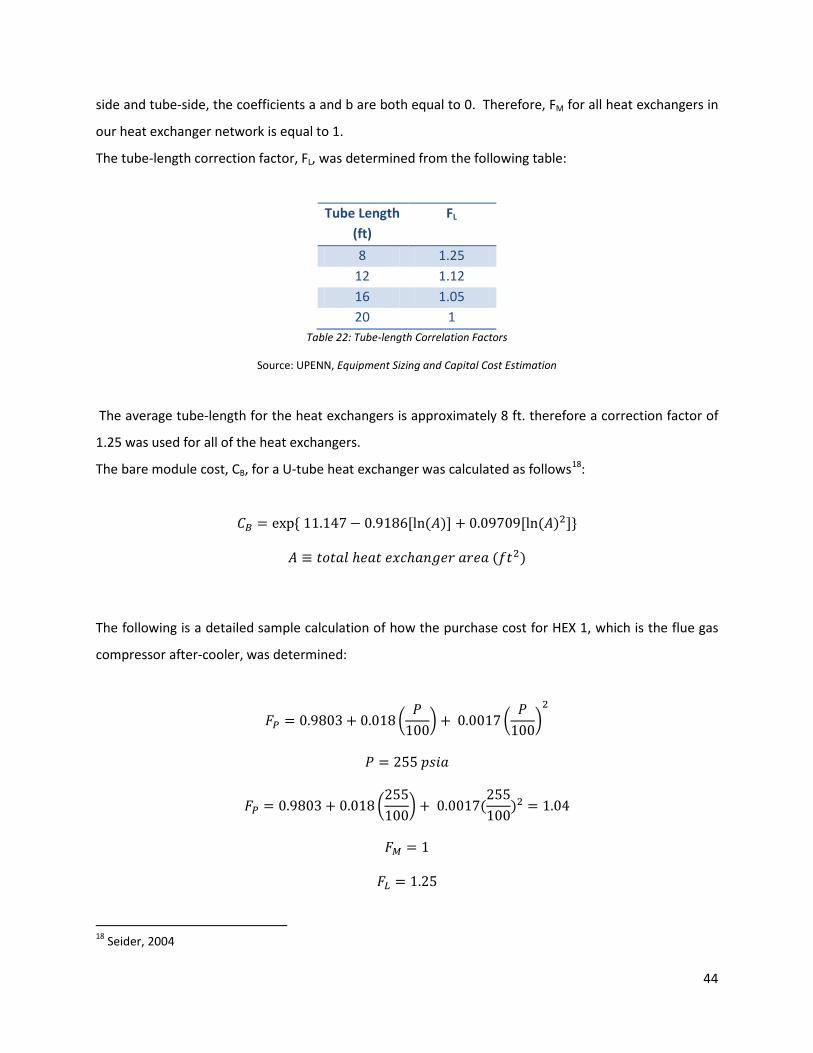
The tube-length correction factor, FL, was determined from the following table:
Tube Length (ft)
FL
8 1.25 12 1.12 16 1.05 20 1
Table 22: Tube-length Correlation Factors
Source: UPENN, Equipment Sizing and Capital Cost Estimation
The average tube-length for the heat exchangers is approximately 8 ft. therefore a correction factor of
1.25 was used for all of the heat exchangers.
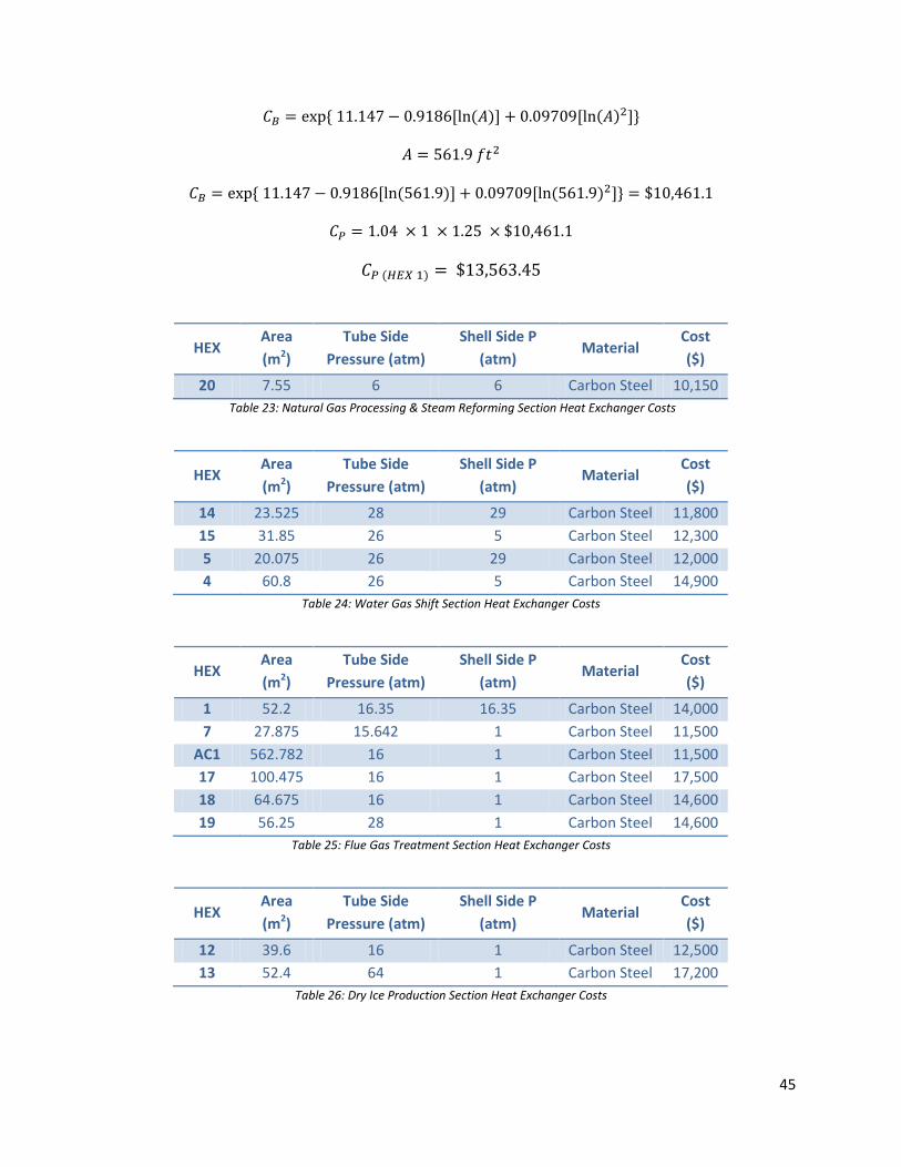
The bare module cost, CB, for a U-tube heat exchanger was calculated as follows18:
𝐶𝐵 = exp{ 11.147− 0.9186[ln(𝐴)] + 0.09709[ln (𝐴)2]}
𝐴 ≡ 𝑡𝑜𝑡𝑎𝑙 ℎ𝑒𝑎𝑡 𝑒𝑥𝑐ℎ𝑎𝑛𝑔𝑒𝑟 𝑎𝑟𝑒𝑎 (𝑓𝑡2)
The following is a detailed sample calculation of how the purchase cost for HEX 1, which is the flue gas
compressor after-cooler, was determined:
𝐹𝑃 = 0.9803 + 0.018 �𝑃
100� + 0.0017 �
𝑃100
�2
𝑃 = 255 𝑝𝑠𝑖𝑎
𝐹𝑃 = 0.9803 + 0.018 �255100
� + 0.0017(255100
)2 = 1.04
𝐹𝑀 = 1
𝐹𝐿 = 1.25
18 Seider, 2004
45
𝐶𝐵 = exp{ 11.147− 0.9186[ln(𝐴)] + 0.09709[ln (𝐴)2]}
𝐴 = 561.9 𝑓𝑡2
𝐶𝐵 = exp{ 11.147− 0.9186[ln(561.9)] + 0.09709[ln (561.9)2]} = $10,461.1
𝐶𝑃 = 1.04 × 1 × 1.25 × $10,461.1
𝐶𝑃 (𝐻𝐸𝑋 1) = $13,563.45
HEX Area (m2)
Tube Side Pressure (atm)
Shell Side P (atm)
Material Cost ($)
20 7.55 6 6 Carbon Steel 10,150 Table 23: Natural Gas Processing & Steam Reforming Section Heat Exchanger Costs
HEX Area (m2)
Tube Side Pressure (atm)
Shell Side P (atm)
Material Cost ($)
14 23.525 28 29 Carbon Steel 11,800 15 31.85 26 5 Carbon Steel 12,300 5 20.075 26 29 Carbon Steel 12,000 4 60.8 26 5 Carbon Steel 14,900
Table 24: Water Gas Shift Section Heat Exchanger Costs
HEX Area (m2)
Tube Side Pressure (atm)
Shell Side P (atm)
Material Cost ($)
1 52.2 16.35 16.35 Carbon Steel 14,000 7 27.875 15.642 1 Carbon Steel 11,500
AC1 562.782 16 1 Carbon Steel 11,500 17 100.475 16 1 Carbon Steel 17,500 18 64.675 16 1 Carbon Steel 14,600 19 56.25 28 1 Carbon Steel 14,600
Table 25: Flue Gas Treatment Section Heat Exchanger Costs
HEX Area (m2)
Tube Side Pressure (atm)
Shell Side P (atm)
Material Cost ($)
12 39.6 16 1 Carbon Steel 12,500 13 52.4 64 1 Carbon Steel 17,200
Table 26: Dry Ice Production Section Heat Exchanger Costs
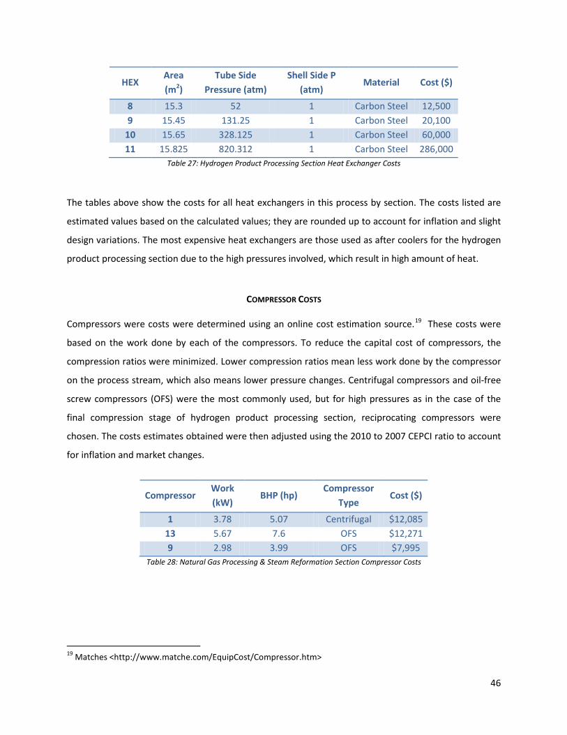
46
HEX Area (m2)
Tube Side Pressure (atm)
Shell Side P (atm)
Material Cost ($)
8 15.3 52 1 Carbon Steel 12,500 9 15.45 131.25 1 Carbon Steel 20,100
10 15.65 328.125 1 Carbon Steel 60,000 11 15.825 820.312 1 Carbon Steel 286,000
Table 27: Hydrogen Product Processing Section Heat Exchanger Costs
The tables above show the costs for all heat exchangers in this process by section. The costs listed are
estimated values based on the calculated values; they are rounded up to account for inflation and slight
design variations. The most expensive heat exchangers are those used as after coolers for the hydrogen
product processing section due to the high pressures involved, which result in high amount of heat.
COMPRESSOR COSTS Compressors were costs were determined using an online cost estimation source.19 These costs were
based on the work done by each of the compressors. To reduce the capital cost of compressors, the
compression ratios were minimized. Lower compression ratios mean less work done by the compressor
on the process stream, which also means lower pressure changes. Centrifugal compressors and oil-free
screw compressors (OFS) were the most commonly used, but for high pressures as in the case of the
final compression stage of hydrogen product processing section, reciprocating compressors were
chosen. The costs estimates obtained were then adjusted using the 2010 to 2007 CEPCI ratio to account
for inflation and market changes.
Compressor Work (kW)
BHP (hp) Compressor
Type Cost ($)
1 3.78 5.07 Centrifugal $12,085 13 5.67 7.6 OFS $12,271 9 2.98 3.99 OFS $7,995
Table 28: Natural Gas Processing & Steam Reformation Section Compressor Costs
19 Matches <http://www.matche.com/EquipCost/Compressor.htm>
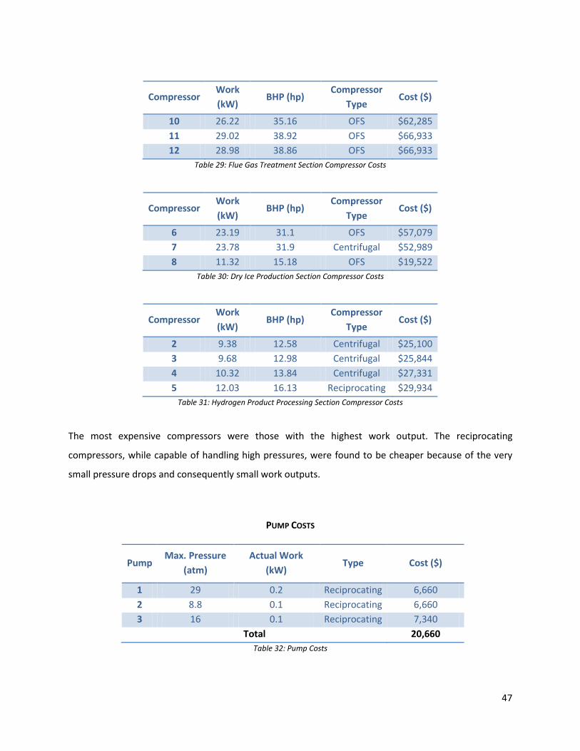
47
Compressor Work (kW)
BHP (hp) Compressor
Type Cost ($)
10 26.22 35.16 OFS $62,285 11 29.02 38.92 OFS $66,933 12 28.98 38.86 OFS $66,933
Table 29: Flue Gas Treatment Section Compressor Costs
Compressor Work (kW)
BHP (hp) Compressor
Type Cost ($)
6 23.19 31.1 OFS $57,079 7 23.78 31.9 Centrifugal $52,989 8 11.32 15.18 OFS $19,522
Table 30: Dry Ice Production Section Compressor Costs
Compressor Work (kW)
BHP (hp) Compressor
Type Cost ($)
2 9.38 12.58 Centrifugal $25,100 3 9.68 12.98 Centrifugal $25,844 4 10.32 13.84 Centrifugal $27,331 5 12.03 16.13 Reciprocating $29,934
Table 31: Hydrogen Product Processing Section Compressor Costs
The most expensive compressors were those with the highest work output. The reciprocating
compressors, while capable of handling high pressures, were found to be cheaper because of the very
small pressure drops and consequently small work outputs.
PUMP COSTS
Pump Max. Pressure
(atm) Actual Work
(kW) Type Cost ($)
1 29 0.2 Reciprocating 6,660 2 8.8 0.1 Reciprocating 6,660 3 16 0.1 Reciprocating 7,340
Total 20,660 Table 32: Pump Costs
48
Pump costs could not be directly calculated based on the work because of the low work values and
volumes. All calculated costs were overestimates and as a result an alternate method of estimating costs
was required. Pump costs were estimated using Matche.20 In general, the pump costs were very small
due to the small volumes of the process stream being pumped. In addition, the work required for each
of the pumps was also very small. The pump costs are summarized above in Table 32.
TANK COSTS
Initial cost estimates based on CAPCOST21 data and design relations yielded inaccurate costs. While
generally accurate for average tanks and vessels, the vessels for this process are quite small. The original
costs calculated were extremely large given the size of the tanks. As a result, the costs were determined
using a ratio; the following relation was used to scale down prices of larger tanks.
𝐶1 = 𝐶2 �𝑉2𝑉1�0.7
For a tank of volume 7.57 m3 (2000 gallons), the cost was determined using the chemical engineering
cost estimation resource Matches.22
𝐶1 = 46700 �0.0045
7.57�0.7
𝐶1 = $258
The cost of the dry ice flash was found to be approximately $258. The total cost of all 5 flash tanks was
estimated to be $1800. The hydrogen storage tank costs were estimated using the same relation. The
cost of one vessel was found to be $7165. Since 24 vessels are required the total cost will be
approximately $172,000. The total cost of all flash tanks and storage vessels was found to be
approximately $190,000.
20 Matche <http://www.matche.com/EquipCost/PumpCentr.htm> 21 Turton et al., 2003 22 Matche <http://www.matche.com/EquipCost/Tank.htm>
49
UTILITY COSTS Costing of utilities required utility consumption values given by PRO/II based on the design of reactors,
heat exchangers, pumps, and separation units.
In general, the following relationship can be used to determine the annual cost of utilities given the
consumption on an hourly basis:
𝐶𝑜𝑠𝑡 = 𝑐𝑜𝑛𝑠𝑢𝑚𝑝𝑡𝑖𝑜𝑛 (𝑝𝑒𝑟 𝑢𝑛𝑖𝑡 𝑡𝑖𝑚𝑒) × 𝑢𝑛𝑖𝑡 𝑐𝑜𝑠𝑡
𝐶𝑜𝑠𝑡 𝑝𝑒𝑟 𝑦𝑒𝑎𝑟 = 𝑐𝑜𝑛𝑠𝑢𝑚𝑝𝑡𝑖𝑜𝑛 (𝑝𝑒𝑟 ℎ𝑜𝑢𝑟) × 24 ℎ𝑜𝑢𝑟𝑠𝑑𝑎𝑦
×365 𝑑𝑎𝑦𝑠𝑦𝑒𝑎𝑟
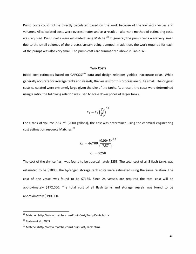
Water kg/hr m3/hr gal/hr $/1000 gal $/hr $/yr
Feed 344.092 0.345 91.173
0.08
0.0073 58.35 Cooling 3562.241 3.573 943.876 0.0755 604.08
NG Comp. 82.761 0.083 21.929 0.0018 14.03 H2 Comp. 609.741 0.612 161.561 0.0129 103.40
Flue Comp. 1946.546 1.952 515.770 0.0413 330.09 CO2 Comp. 923.194 0.926 244.616 0.0196 156.55
Total 662.43 Table 33: Water Costs
Table 33 shows the total water usage for each section or component with a water requirement. The unit
cost of water (current sale price) is $0.08 per thousand gallons. The process has been designed
minimized water usage and as a result, the cost of water per year is only approximately $663, which is a
relatively low amount especially in comparison with natural gas costs show below in Table 34.
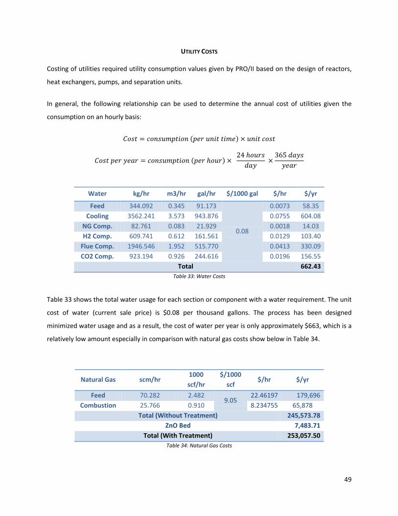
Natural Gas scm/hr 1000 scf/hr
$/1000 scf
$/hr $/yr
Feed 70.282 2.482 9.05
22.46197 179,696 Combustion 25.766 0.910 8.234755 65,878
Total (Without Treatment) 245,573.78 ZnO Bed 7,483.71
Total (With Treatment) 253,057.50 Table 34: Natural Gas Costs
50
A large contribution to overall costs is the natural gas feed. The market cost of natural gas is
approximately $2 per thousand gallons. The large volume of natural gas required to meet the
production requirement and the market demand of hydrogen results in an annual natural gas
expenditure of approximately $54,270. Another cost that arises because of the use of natural gas feed is
the cost of the pretreatment. The ZnO bed contributes greatly to the total cost both by design and
because of the adsorbent requirement. Table 34 shows the breakdown of natural gas usage and costs.
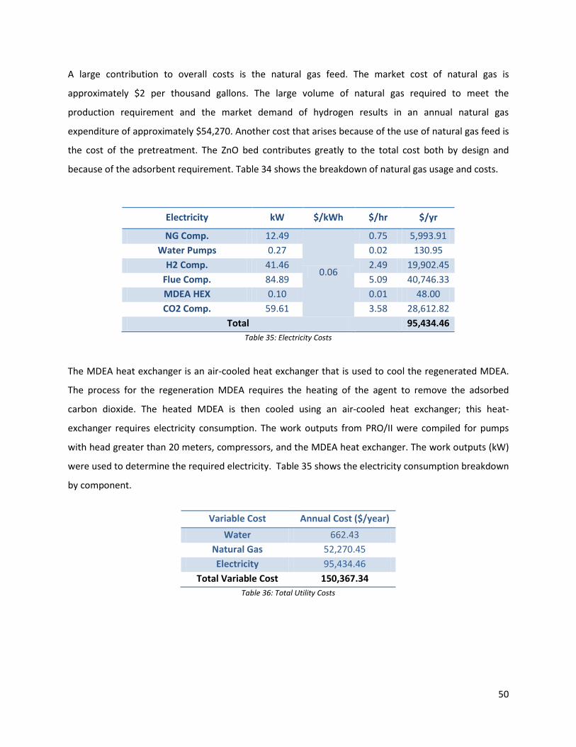
Electricity kW $/kWh $/hr $/yr
NG Comp. 12.49
0.06
0.75 5,993.91 Water Pumps 0.27 0.02 130.95
H2 Comp. 41.46 2.49 19,902.45 Flue Comp. 84.89 5.09 40,746.33 MDEA HEX 0.10 0.01 48.00 CO2 Comp. 59.61 3.58 28,612.82
Total
95,434.46 Table 35: Electricity Costs
The MDEA heat exchanger is an air-cooled heat exchanger that is used to cool the regenerated MDEA.
The process for the regeneration MDEA requires the heating of the agent to remove the adsorbed
carbon dioxide. The heated MDEA is then cooled using an air-cooled heat exchanger; this heat-
exchanger requires electricity consumption. The work outputs from PRO/II were compiled for pumps
with head greater than 20 meters, compressors, and the MDEA heat exchanger. The work outputs (kW)
were used to determine the required electricity. Table 35 shows the electricity consumption breakdown
by component.
Variable Cost Annual Cost ($/year)
Water 662.43 Natural Gas 52,270.45 Electricity 95,434.46
Total Variable Cost 150,367.34 Table 36: Total Utility Costs
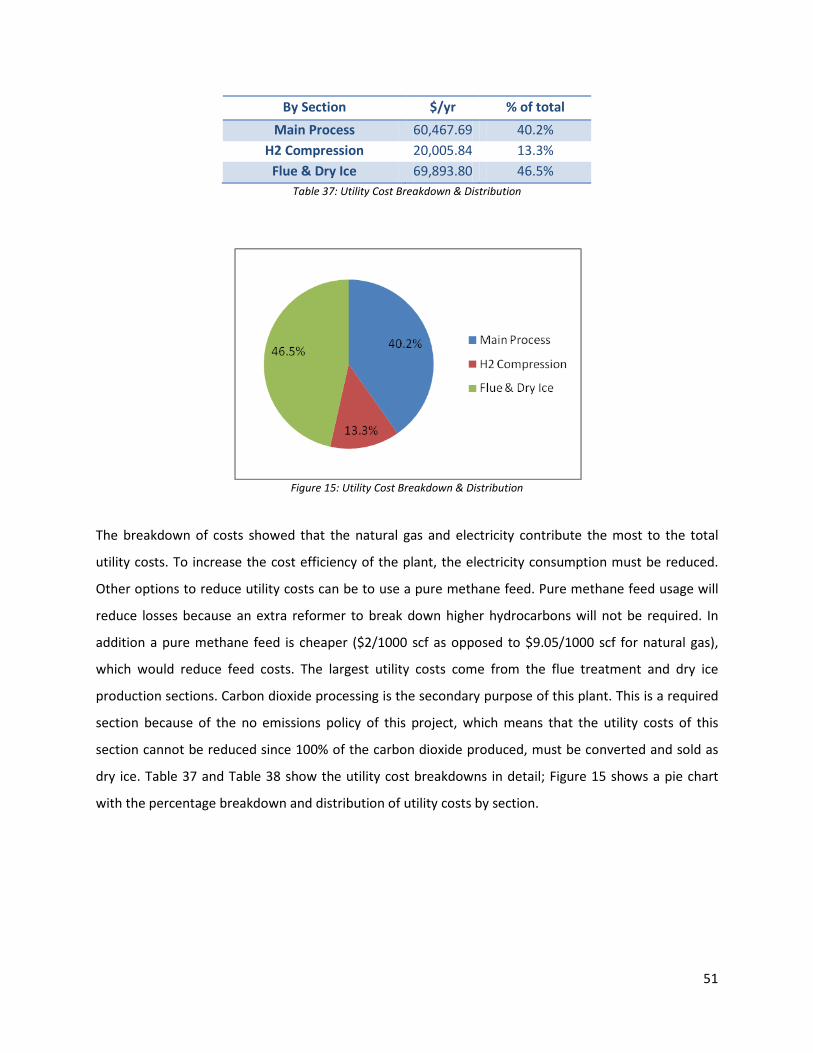
51
By Section $/yr % of total Main Process 60,467.69 40.2%
H2 Compression 20,005.84 13.3% Flue & Dry Ice 69,893.80 46.5%
Table 37: Utility Cost Breakdown & Distribution
Figure 15: Utility Cost Breakdown & Distribution
The breakdown of costs showed that the natural gas and electricity contribute the most to the total
utility costs. To increase the cost efficiency of the plant, the electricity consumption must be reduced.
Other options to reduce utility costs can be to use a pure methane feed. Pure methane feed usage will
reduce losses because an extra reformer to break down higher hydrocarbons will not be required. In
addition a pure methane feed is cheaper ($2/1000 scf as opposed to $9.05/1000 scf for natural gas),
which would reduce feed costs. The largest utility costs come from the flue treatment and dry ice
production sections. Carbon dioxide processing is the secondary purpose of this plant. This is a required
section because of the no emissions policy of this project, which means that the utility costs of this
section cannot be reduced since 100% of the carbon dioxide produced, must be converted and sold as
dry ice. Table 37 and Table 38 show the utility cost breakdowns in detail; Figure 15 shows a pie chart
with the percentage breakdown and distribution of utility costs by section.
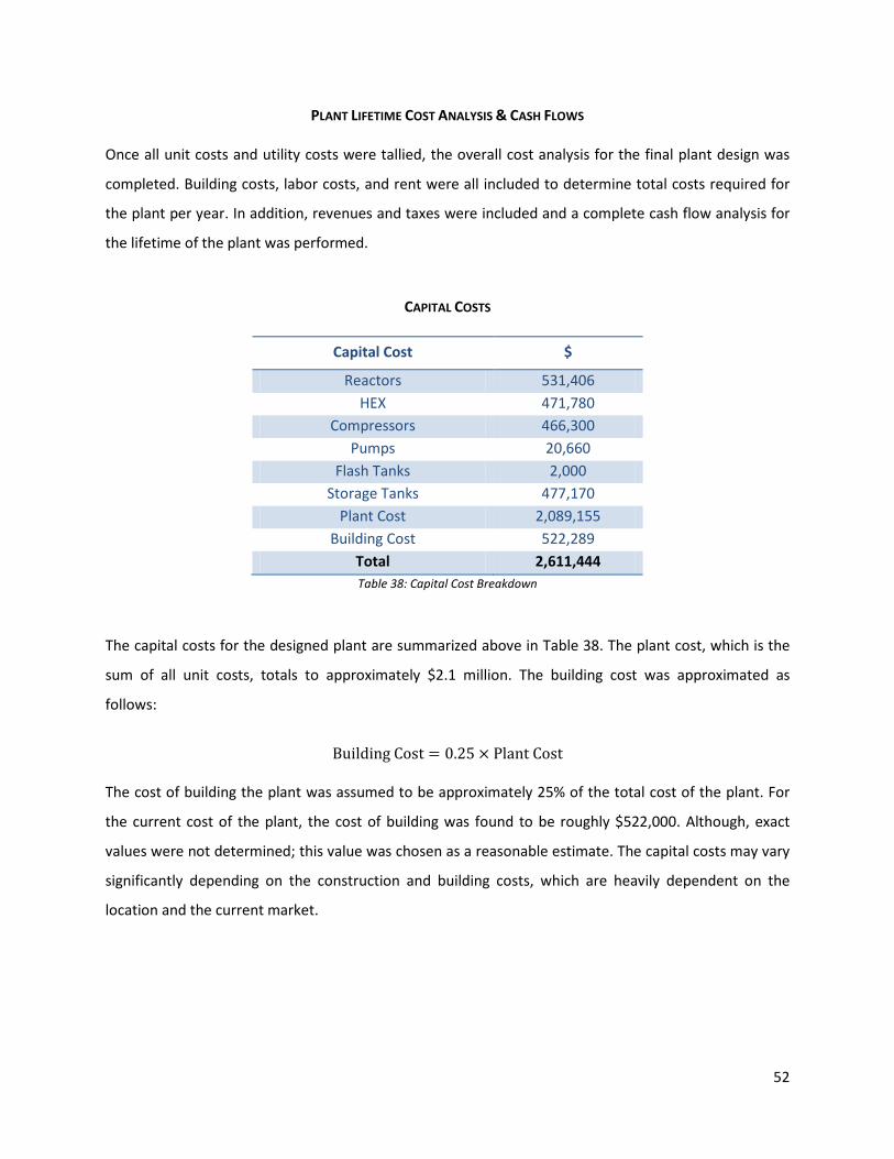
52
PLANT LIFETIME COST ANALYSIS & CASH FLOWS Once all unit costs and utility costs were tallied, the overall cost analysis for the final plant design was
completed. Building costs, labor costs, and rent were all included to determine total costs required for
the plant per year. In addition, revenues and taxes were included and a complete cash flow analysis for
the lifetime of the plant was performed.
CAPITAL COSTS
Capital Cost $
Reactors 531,406 HEX 471,780
Compressors 466,300 Pumps 20,660
Flash Tanks 2,000 Storage Tanks 477,170
Plant Cost 2,089,155 Building Cost 522,289
Total 2,611,444 Table 38: Capital Cost Breakdown
The capital costs for the designed plant are summarized above in Table 38. The plant cost, which is the
sum of all unit costs, totals to approximately $2.1 million. The building cost was approximated as
follows:
Building Cost = 0.25 × Plant Cost
The cost of building the plant was assumed to be approximately 25% of the total cost of the plant. For
the current cost of the plant, the cost of building was found to be roughly $522,000. Although, exact
values were not determined; this value was chosen as a reasonable estimate. The capital costs may vary
significantly depending on the construction and building costs, which are heavily dependent on the
location and the current market.
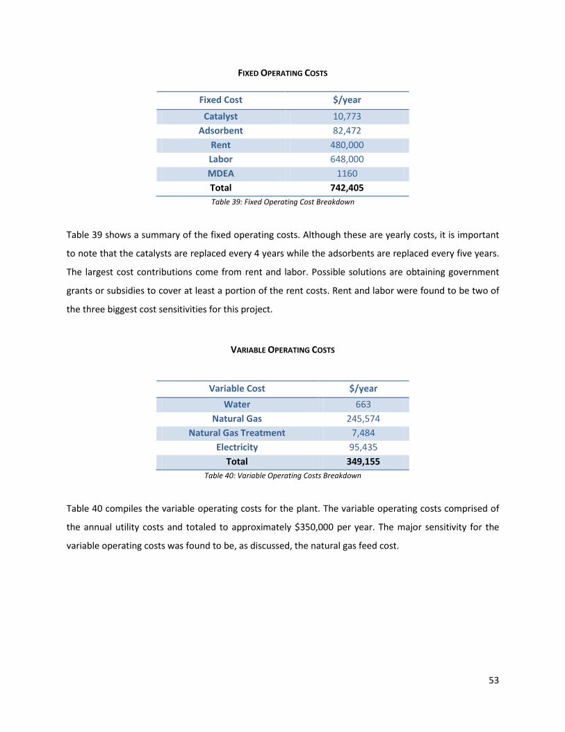
53
FIXED OPERATING COSTS
Fixed Cost $/year
Catalyst 10,773 Adsorbent 82,472
Rent 480,000 Labor 648,000 MDEA 1160 Total 742,405 Table 39: Fixed Operating Cost Breakdown
Table 39 shows a summary of the fixed operating costs. Although these are yearly costs, it is important
to note that the catalysts are replaced every 4 years while the adsorbents are replaced every five years.
The largest cost contributions come from rent and labor. Possible solutions are obtaining government
grants or subsidies to cover at least a portion of the rent costs. Rent and labor were found to be two of
the three biggest cost sensitivities for this project.
VARIABLE OPERATING COSTS
Variable Cost $/year Water 663
Natural Gas 245,574 Natural Gas Treatment 7,484
Electricity 95,435 Total 349,155
Table 40: Variable Operating Costs Breakdown
Table 40 compiles the variable operating costs for the plant. The variable operating costs comprised of
the annual utility costs and totaled to approximately $350,000 per year. The major sensitivity for the
variable operating costs was found to be, as discussed, the natural gas feed cost.
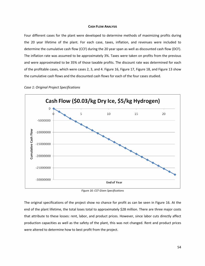
54
CASH FLOW ANALYSIS Four different cases for the plant were developed to determine methods of maximizing profits during
the 20 year lifetime of the plant. For each case, taxes, inflation, and revenues were included to
determine the cumulative cash flow (CCF) during the 20 year span as well as discounted cash flow (DCF).
The inflation rate was assumed to be approximately 3%. Taxes were taken on profits from the previous
and were approximated to be 35% of those taxable profits. The discount rate was determined for each
of the profitable cases, which were cases 2, 3, and 4. Figure 16, Figure 17, Figure 18, and Figure 13 show
the cumulative cash flows and the discounted cash flows for each of the four cases studied.
Case 1: Original Project Specifications
Figure 16: CCF Given Specifications
The original specifications of the project show no chance for profit as can be seen in Figure 16. At the
end of the plant lifetime, the total loses total to approximately $28 million. There are three major costs
that attribute to these losses: rent, labor, and product prices. However, since labor cuts directly affect
production capacities as well as the safety of the plant, this was not changed. Rent and product prices
were altered to determine how to best profit from the project.
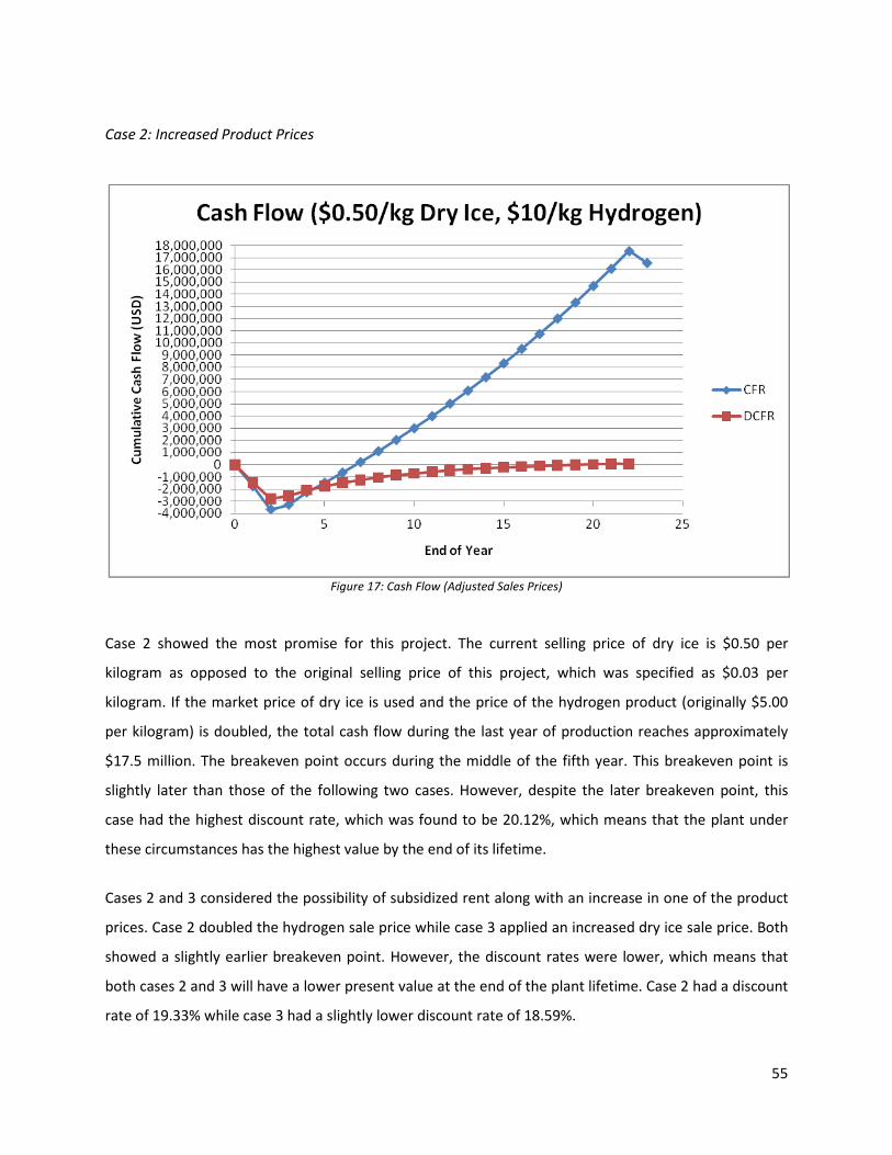
55
Case 2: Increased Product Prices
Figure 17: Cash Flow (Adjusted Sales Prices) Case 2 showed the most promise for this project. The current selling price of dry ice is $0.50 per
kilogram as opposed to the original selling price of this project, which was specified as $0.03 per
kilogram. If the market price of dry ice is used and the price of the hydrogen product (originally $5.00
per kilogram) is doubled, the total cash flow during the last year of production reaches approximately
$17.5 million. The breakeven point occurs during the middle of the fifth year. This breakeven point is
slightly later than those of the following two cases. However, despite the later breakeven point, this
case had the highest discount rate, which was found to be 20.12%, which means that the plant under
these circumstances has the highest value by the end of its lifetime.
Cases 2 and 3 considered the possibility of subsidized rent along with an increase in one of the product
prices. Case 2 doubled the hydrogen sale price while case 3 applied an increased dry ice sale price. Both
showed a slightly earlier breakeven point. However, the discount rates were lower, which means that
both cases 2 and 3 will have a lower present value at the end of the plant lifetime. Case 2 had a discount
rate of 19.33% while case 3 had a slightly lower discount rate of 18.59%.
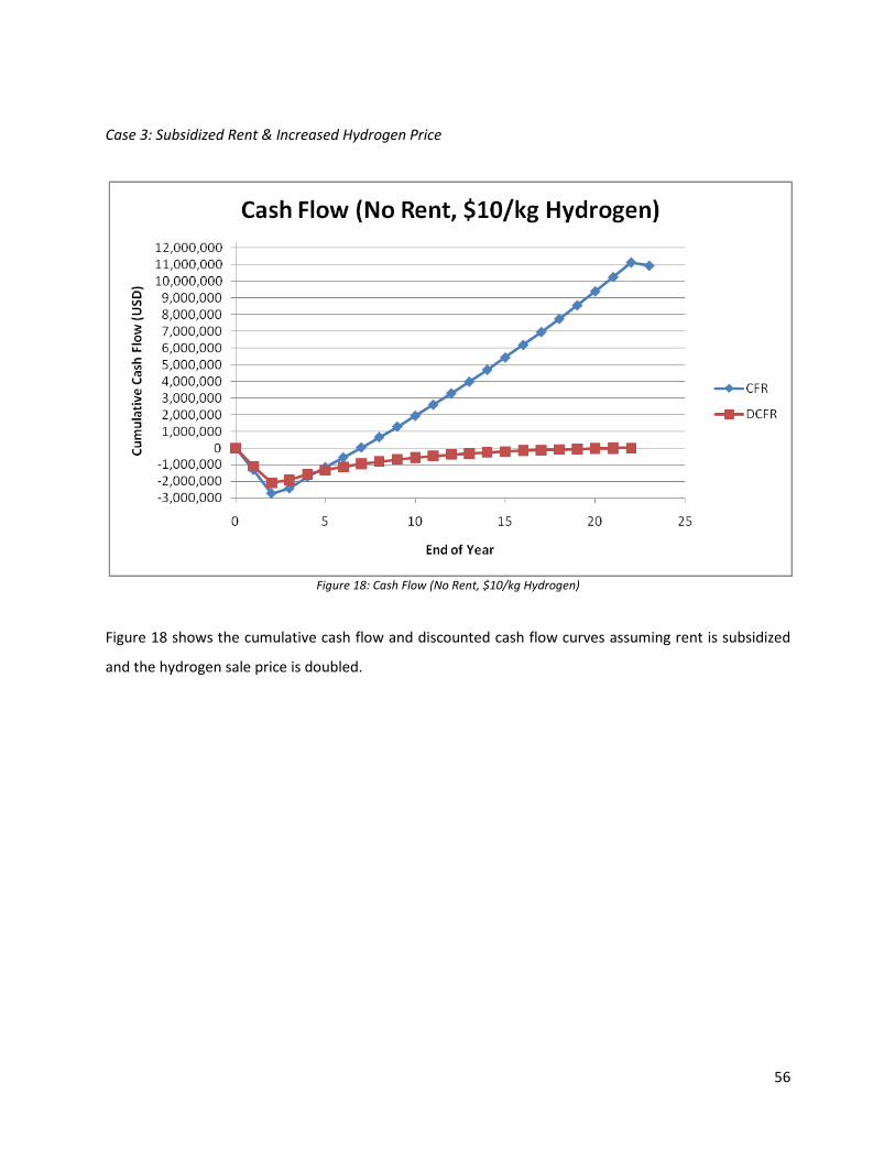
56
Case 3: Subsidized Rent & Increased Hydrogen Price
Figure 18: Cash Flow (No Rent, $10/kg Hydrogen)
Figure 18 shows the cumulative cash flow and discounted cash flow curves assuming rent is subsidized
and the hydrogen sale price is doubled.
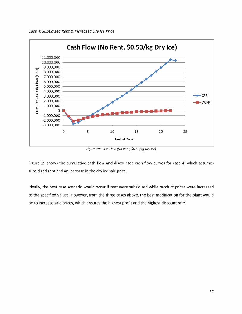
57
Case 4: Subsidized Rent & Increased Dry Ice Price
Figure 19: Cash Flow (No Rent, $0.50/kg Dry Ice)
Figure 19 shows the cumulative cash flow and discounted cash flow curves for case 4, which assumes
subsidized rent and an increase in the dry ice sale price.
Ideally, the best case scenario would occur if rent were subsidized while product prices were increased
to the specified values. However, from the three cases above, the best modification for the plant would
be to increase sale prices, which ensures the highest profit and the highest discount rate.
58
OBJECTIVES
PROCESS DESIGN The main process objective of this project was to design a production plant that converted natural gas
into H2 product of 99.9999% purity. Our goal for H2 production capacity was to produce enough H2 to
meet a fueling rate of 100 vehicles per day with a tank size specification of 4 kg at 700 atm. The goal for
storage capacity was to store enough H2 product for approximately 766 hours. Our success in achieving
the desired purity of H2 product was measured by analyzing the composition of the exit H2 product
stream from the final purification stage of the production process. Our success in achieving the
production rate and storage capacity goals was measured by determining the amount of H2 product
yielded in our final plant design process and determining whether it satisfied both the production and
storage capacity requirements.
Another process objective of this project was to design a H2 production process with high process
efficiency. Our criteria for an efficient process were the following: an actual H2 yield close to the
maximum theoretical yield, minimal utility consumption and energy input, and high recycle of waste
product streams. Our success in achieving this objective was measured by comparing our plant to other
H2 production plants and determining which plant satisfied our criteria the best.
ECONOMICS
The primary economic objective of this project was to design a plant that would earn profit before the
midpoint of the lifetime of the plant. Our success in achieving this objective was measured by
performing a complete cost analysis of the plant and determining the breakeven point for the plant’s
cumulative cash flow over its lifetime.
ENVIRONMENTAL & SAFETY FACTORS
The primary environmental objective of this project was to design a plant with zero carbon dioxide
(CO2), carbon monoxide (CO), and hydrogen sulfide (H2S) emissions. Our plant is designed for zero CO2
emissions because CO2 is a heat-trapping greenhouse gas (GHG). Our plant is designed for zero CO and
H2S emissions because CO and H2S are classified by the EPA as toxic and hazardous wastes respectively.
Our success in achieving the zero emissions objectives was measured by determining the amount of CO2,
CO, and H2S yielded in our final plant design process.
The primary safety objective of this project was to design the physical layout of our plant in a way that
minimized safety risks associated with our plant. Our success in achieving a plant design that had

59
minimal safety risks was measured by determining all of the safety risks posed by the plant and then
determining how many safety risks were minimized as a result of the safety precautions that were
implemented in our design.
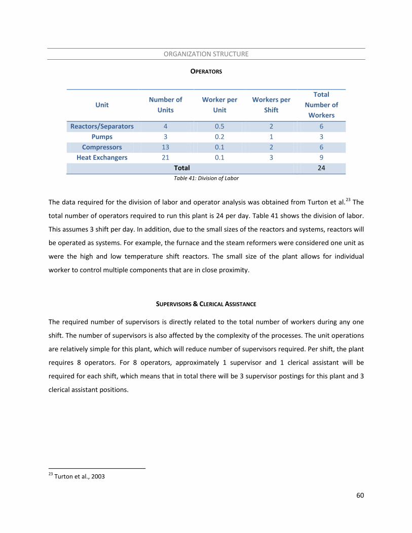
60
ORGANIZATION STRUCTURE
OPERATORS
Unit Number of
Units Worker per
Unit Workers per
Shift
Total Number of
Workers Reactors/Separators 4 0.5 2 6
Pumps 3 0.2 1 3 Compressors 13 0.1 2 6
Heat Exchangers 21 0.1 3 9 Total 24 Table 41: Division of Labor
The data required for the division of labor and operator analysis was obtained from Turton et al.23 The
total number of operators required to run this plant is 24 per day. Table 41 shows the division of labor.
This assumes 3 shift per day. In addition, due to the small sizes of the reactors and systems, reactors will
be operated as systems. For example, the furnace and the steam reformers were considered one unit as
were the high and low temperature shift reactors. The small size of the plant allows for individual
worker to control multiple components that are in close proximity.
SUPERVISORS & CLERICAL ASSISTANCE The required number of supervisors is directly related to the total number of workers during any one
shift. The number of supervisors is also affected by the complexity of the processes. The unit operations
are relatively simple for this plant, which will reduce number of supervisors required. Per shift, the plant
requires 8 operators. For 8 operators, approximately 1 supervisor and 1 clerical assistant will be
required for each shift, which means that in total there will be 3 supervisor postings for this plant and 3
clerical assistant positions.
23 Turton et al., 2003
61
QUALITY CONTROL PLAN
Quality control is a very important aspect of this project because the cost per kilogram of hydrogen is
very high, which means that the product must meet the market standards of this project. Hydrogen
must be sampled regularly and analyzed to ensure that the purity is 99.9999%. The best method of
testing the samples is by using gas chromatography mass spectrometry (GCMS). It is reccomended that
the project investment includes the purchase of a GCMS. This is a valuable investment because samples
must be taken from the process and analyzed three times a day. At the beginning of every shift, the
operator in charge of the hydrogen storage tanks must sample the product and analyze it using the
GCMS. The sampling and testing must occur three times a day because the plant only has an excess
storage capacity of one day, which means that quality control must be accounted for at all times. Impure
product would result in significant loss of revenue. Operators in charge of the hydrogen storage must be
trained to take the appropriate sized samples and run the GCMS. GCMS outputs must also be accurately
read in order to determine the quality and composition of product. All operators must be trained to use
the GCMS in order to understand how individual unit operations affect the product and the sample
readings. All operators must also be trained to make adjustments immediately as needed depending on
the GCMS output.
62
HEALTH & SAFETY PLAN
Safety precautions were taken in the design of the plant to assure minimal risk to employees of our H2
production plant. A major safety risk associated with our plant is the leakage of poisonous gases from
process equipment due to failures in the equipment. The primary gases of concern are H2S and CO.
H2S is a flammable, toxic, and hazardous gas that has a strong characteristic odor of rotten eggs.
The exposure pathways for H2S are inhalation and dermal. If inhaled in high concentrations, H2S can
cause unconsciousness, coma, or even death. Dermal contact with H2S can cause irritation to the skin in
the form of frostbite. To prevent emissions of H2S from the plant, excess ZnO adsorbent is used in the
pre-treatment stage of the H2 production process to assure complete removal of H2S from the natural
gas feedstock. The adsorbent must be replaced annually to maintain its complete loading performance.
Since H2S is classified by the US EPA as hazardous waste, the employees of the plant that work in the
pre-treatment stage of the plant must have proper training in hazardous waste disposal and be
educated on the regulations for hazardous waste handling established by the Resource and Recovery
Act (RCRA). Employees will be required to wear protective eye wear, thermally insulated gloves, static
resistant clothes, and safety shoes when handling containers of the H2S. Detectors for H2S are attached
to process equipment in the pre-treatment stage. Automatic monitoring equipment for oxygen and the
presence of potentially explosive air-gas mixtures is also installed in the pre-treatment stage and
throughout the plant. Local exhaust ventilation has been implemented in the plant design to ensure
that H2S does not exceed exposure limits to employees working in the plant.
In the case a leakage does occur, the employees will be trained on how to respond
appropriately to the emergency with regards to who to call, fire fighting measures to be taken in the
case of a fire, accidental release measures to be taken, and first aid measures in the case someone does
get injured. Material Safety Data Sheets (MSDS) for hydrogen sulfide will be provided to all employees
and will be located near process equipment in the pre-treatment stage. Fire extinguishers will also be
located throughout the pre-treatment stage and the rest of the plant since our production plant deals
with extremely flammable gases.
CO is a toxic, colorless, and odorless gas. The exposure pathways for CO are inhalation and
dermal. If inhaled, CO exposure can cause target organ damage and even fatality if inhaled in high
concentration. Dermal contact with CO can cause frostbite or burns to the skin. To prevent CO
emissions from the plant, our plant has been designed to convert all intermediate CO into CO2 and H2 in
the temperature shift reaction stages. CO that is not converted in this stage of the process is recovered
in the PSA. The PSA adsorbent will be replaced every four years to maintain optimal performance and
63
complete loading of CO. Employees that will dispose of the PSA adsorbent will be trained in proper
handling methods of CO. All employees that will work in stages of the process where CO can be emitted
will be required to wear properly fitted air-purifying or air-fed respirators, safety eyewear, chemically
resistant and impervious gloves, and chemically resistant clothing. Local exhaust ventilation has been
incorporated in the design of the plant and CO detectors are attached to the reformer, HTS, and LTS
reactors as well as the PSA. The same emergency response measures and training will be taken in the
case of a CO leakage as for a H2S leakage.
Another major safety risk of our plant is the potential for explosions to occur due to the high
temperature and high pressure operating conditions of the equipment and the high flammability of the
gases that they contain. The reactors of the plant, especially the steam reformers, are operated at
extremely high temperatures. Materials of construction for these high temperature reactors are
thermally resistant and therefore will not melt under the reactor operating conditions. Temperature
detectors are attached to all process equipment to monitor the internal temperatures of the equipment.
Control engineers will be employed at our plant and will monitor the operating temperatures and
pressures of all process equipment in the plant. They will be trained on how to respond if the
temperatures or pressures exceed the maximum of the safe operating range for each type of
equipment. Equipment that operates at high pressures will be double-contained to avoid material
failure and consequently a possible explosion. Routine inspections of process equipment will be made
by plant engineers in order to identify any failures in the equipment and take immediate action to fix
any mechanical failures.
Since our plant deals with highly flammable gases, it is important to eliminate exposure of these
gases to oxygen in the air. Therefore, most of the major equipment in our plant will be located
underground to avoid risks of explosion.
64
ENVIRONMENTAL HEALTH & SAFETY TARGETS
ENVIRONMENTAL TARGETS
The environmental targets for our H2 production plant are zero H2S, CO, and CO2 emissions and minimal
wastewater production.
The processes involved in our H2 production plant produce H2S, CO, and CO2. H2S is a colorless
gas characterized by its strong rotten egg odor and is classified by the US Environmental Protection
Agency (EPA) as a hazardous waste. H2S naturally occurs in the natural gas feedstock to our production
plant. The total sulfide composition of the natural gas feedstock is approximately 0.2 mol%. The H2S in
the natural gas is removed by adsorption in the ZnO bed prior to the steam reformation stages. ZnO
was chosen as the pre-treatment adsorbent because it can achieve almost complete loading of H2S. In
order to assure that our production plant has zero H2S emissions, we have designed the ZnO bed to hold
more adsorbent than is necessary to treat the amount of natural gas that will be processed in our plant.
Excess adsorbent ensures complete removal of H2S from the natural gas process stream in the pre-
treatment stage and consequently yields zero emissions. To maintain complete loading of H2S on the
ZnO bed, the adsorbent is replaced on a yearly basis.
CO is a toxic gas that is produced in the steam reformation stage of the H2 production process.
CO is a pollutant that contributes to smog formation and the US EPA’s maximum allowable level for CO
in the air is 9 parts per million (ppm). CO is an intermediate product of the H2 production process that is
converted to CO2 and H2 in the temperature shift reaction stages. The CO product from steam
reformation is reacted with steam in the temperature shift reactors at significantly lower temperatures
than steam reformation. The temperature shift reactions favor low temperatures to achieve high
conversion of CO. Therefore, to assure that all CO produced in our plant is converted to H2 and CO2, we
use two temperature shift reactors that operate at different temperature ranges. The CO-rich product
stream from the steam reformer is first processed in a high temperature shift (HTS) reactor and then is
processed through a low temperature shift (LTS) reactor. Since the temperature shift reactions favor
low temperatures for high conversion, the LTS reactor, which operates at a lower temperature range
than the HTS, is used to convert any remaining CO that was not reacted in the HTS. CO that is not
converted by the HTS and LTS is then captured in the pressure swing adsorber (PSA) to ensure that no
CO emissions are made from the plant. To maintain complete loading of CO on the PSA adsorbent, the
adsorbent will be replaced every 4 years.
CO2 is a greenhouse gas that traps heat in the atmosphere and is known to contribute to global
warming. In 2009, the US EPA officially declared CO2 a dangerous air pollutant and established the
65
legislative framework for CO2 regulations on emissions that will be enforced in the upcoming years
under the Clean Air Act. CO2 is produced in the temperature shift reaction stages of the H2 production
process, is separated and recovered from the H2-rich process stream in the PSA, and is recycled for use
as furnace combustion fuel as part of the PSA off-gas. CO2 is a component in the flue gas exit stream of
the furnace. The CO2-rich exit flue gas is processed through the MDEA scrubber which removes 99.5%
CO2 from the flue gas. CO2 is released from the CO2-rich MDEA via heating and is converted into dry ice.
Although the environmental target for the plant is zero CO2 emissions, the MDEA scrubber doesn’t
recover all of the CO2 from the flue gas. Therefore, the plant has emissions rate of 48,000 kg of CO2 per
year in the exit flue gas from the scrubber.
Our H2 production plant generates 283,190 gallons of wastewater per year from condensation
of the process stream. The wastewater is not contaminated with any hazardous or toxic chemicals
therefore it does not need to be treated and does not pose any risks to environmental health.
SAFETY TARGETS
The safety targets for our plant are minimal risk for explosion, prevention of poisonous gas
releases, and minimal safety risk to our workers and residents near the plant site.
H2 is a highly combustible gas when it comes into contact with air therefore precautions were
taken in designing the physical layout of the plant to ensure minimal risk of explosion. The majority of
the equipment for the plant, specifically the compressors, heat exchangers, and hydrogen storage tanks
are located underground. Therefore, if a H2 leak were to occur, there will be less oxygen available
underground to produce a large explosion and less damage to surrounding buildings would occur.
Much of the equipment in our H2 production plant is operated at very high pressures and high
temperatures therefore measures must be taken to prevent explosions that can be caused by
equipment failure. High temperatures in reactors can be dangerous if they exceed the operating range
limit. High temperatures can melt the reactor vessel material which can consequently result in the
release of toxic materials from within the reactor. To avoid this problem, temperature monitors will be
used to make sure that the operating temperatures of a reactor do not exceed the safe operating range.
High operating pressures can also pose safety risks if they exceed the operating limit because they can
cause equipment explosions. To avoid this, all high pressure equipment in our plant has a double layer
of containment.
Our plant site is located in a densely populated residential area in New York City therefore
appropriate measures were taken in the design of our plant and in the training of our employees to
make sure that the residents of the surrounding community are not put at risk as a result of our plant
66
operations. Since our plant produces H2S and CO, both of which are poisonous gases, we modified our
design to achieve zero emissions of these gases. All of the H2S from the process is captured by excess
adsorbent in the pre-treatment stage therefore eliminating the risk of H2S emissions. With regards to
the CO, in the case that there is a leak in our plant equipment, we attached CO detectors to all of the
process equipment. CO is a colorless and odorless gas therefore detectors must be used to determine if
CO leakage has occurred. If the detectors indicate any level of CO, action will be taken to pinpoint the
source of leakage and correct the failure in the equipment.
Proper training of our H2 production plant employees is also essential in reducing safety risks of
the plant. Control engineers will be employed in our plant to monitor the operating conditions of all the
equipment and make sure that the equipment doesn’t malfunction. Routine daily inspections will be
made by plant operations employees to check for any damaged equipment or piping. Fueling station
operators who fuel the vehicles will be trained in proper materials handling. Safety training will be
provided to all our plant employees so that as little damage as possible is caused on the plant and the
surrounding area in the case of an emergency situation.
67
PROJECT REPORTING & REVIEWS
SUPERVISOR GOALS The supervisor is expected to ensure that all goals are met on time. There should be meetings with the
design team weekly to ensure deadlines and goals are met. Once construction begins, weekly meetings
should be scheduled to obtain information about progress and to ensure goals and deadlines are met.
It is important to be aware of the design and constructions that come up. Necessary conferences and
meetings should be scheduled to address problems, questions, and concerns. An open forum must be
scheduled to allow the affected general public to ask questions and raise concerns about the project.
The goal is to have the plant begin producing within 12 months of the first design meeting.
DESIGN TEAM GOALS
Weekly progress reports are required to ensure that all parties involved are updated on the design
progress. Design team must initially have weekly meetings with the supervisor to go over design
progress and discuss any design issues. Design of the plant should be completed within 3 months so that
construction can begin. Once construction begins, the team must meet weekly with the construction
team to ensure goals and deadlines are met. It is important that any design issues during construction
are brought up and managed immediately to avoid delays in the project.
CONSTRUCTION TEAM GOALS
The construction team must begin work immediately after all designs are completed. It is required that
the team meets with the design team weekly with progress reports. All construct and design issues must
be brought immediately to both the design team as well as the supervisor to avoid delays. The
construction of the plant must be completed within 8 months of the month that the design is
completed. 1 month is then allowed for implementation, safety, and environmental checks. The
operation of the plant must begin at the beginning of the following year.

68
PRODUCTION GOALS The reactors and separators must be constructed by the end of the fourth month of construction. The
remaining time will be allotted for the implementation of pumps, compressors, pipelines, storage tanks,
flash tanks, and safety components. The plant, during the first year, will have a production rate of 75%
capacity. By the second year, the plant must be operating at 100% capacity.
69
PROJECT ENHANCEMENT STRATEGIES
From our design and economic analysis of the NYC Hydrogen Fueling Station, we have determined that
the plant is profitable for increased sale prices or reduced rent. However, the performance and
profitability of the plant can be improved during operation with both process improvements and
economic decisions.
Process improvements proposals should be developed during times of normal operation when there are
no maintenance issues. Process engineers will meet once a week to discuss potential modifications or
upgrades to the plant that can improve its performance. For example, a proposed modification may be
to change the PSA adsorbent from pure zeolite 5A to a mixture of zeolite 5A and activated carbon. The
discussion of this modification will evaluate the cost savings from changing the adsorbent and the
impact it will have on the product quality, if any. If a process modification is agreed upon, a strategy for
implementing the modification will be developed to minimize the plant shut-down time required. An
important factor in evaluating a process improvement is the impact it may have on the hydrogen supply
to the customers. In particular, if the improvement requires less than 24 hours of shutdown time,
hydrogen should still be continuously available to the customers.
Ongoing market research should be performed by the marketing department to determine proper
pricing of the products. The hydrogen sale price should be set competitively compared to the prices of
nearby fueling stations. The plant is currently designed to produce a small surplus of hydrogen in
addition to that being sold as on-site vehicle fuel. During periods of reduced customers (i.e. the winter
season) it may be profitable to sell the surplus hydrogen to other markets, such as ammonia production.
Finally, the hydrogen fuel economy is frequently subsidized by the government due to the push towards
cleaner vehicle fuels. Thus, every effort should be made to apply for additional government subsidies
during plant operation.
70
REFERENCES
Green, WD (ed.); Perry, RH (ed.). (2008). Perry’s Chemical Engineer’s Handbook.
Gregory, JD. (2000). Select the right compressor. Chemical Engineering Progress, 96(7): 15-29.
Matches. Matches' Process Equipment Cost Estimates. Last updated 15 Oct 2003.
< http://www.matche.com/EquipCost/index.htm>
Keiski, RL; Salmi, T; Niemistö, P; Ainassaari, J; Pohjola, VJ. (1995). Stationary and transient kinetics of the high
temperature water-gas shift reaction. Applied Catalysis A: General, 137: 349-370.
Posey, ML; Tapperson, KG; Rochelle, GT. (1996). A simple model for prediction of acid gas solubilities in
alkanolamines. Gas Separation and Purification, 10: 181-186.
Rase, HF. (1991). “Case Study 105,” Chemical Reactor Design for Process Plants, 2: 44-60.
Schlünder, EU (ed.). (1993). VDI Heat Atlas, Woodhead Publishing, Limited, Chapter Cc.
Seider, W. (2004). Equipment Sizing and Capital Cost Estimation. Product and Process Design. University
of Pennsylvania, Web.
Sperle, T; Chen, D; Lødeng, R; Holmen, A. (2005). Pre-reforming of natural gas on a Ni catalyst – criteria
for carbon free operation. Applied Catalysis A: General, 282: 195-204.
Turton, R; Bailie, RC; Whiting, WB; Shaeiwitz, JA. (2003). Analysis, Synthesis, and Design of Chemical
Processes, 2/e. Prentice Hall.
Xu, J; Froment, GF. (1989). Methane steam reforming, methanation and water-gas shift: I. Intrinsic
kinetics. AIChE Journal, 35(1): 88-96.
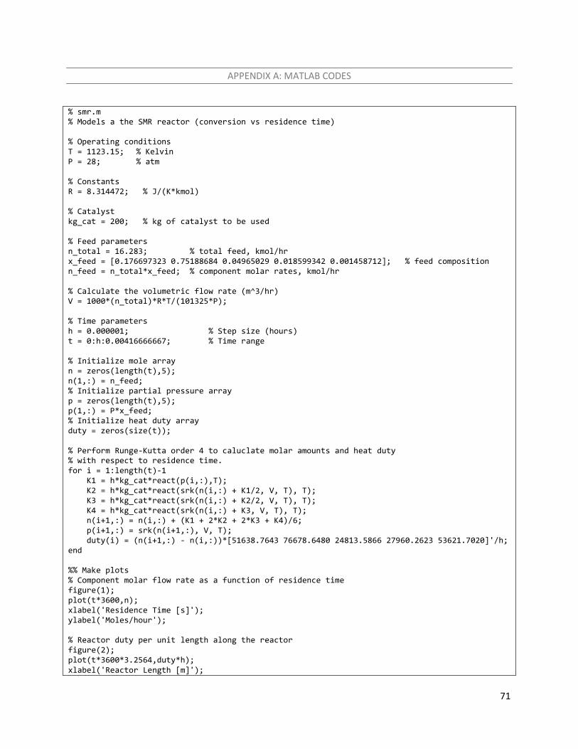
71
APPENDIX A: MATLAB CODES
% smr.m % Models a the SMR reactor (conversion vs residence time) % Operating conditions T = 1123.15; % Kelvin P = 28; % atm % Constants R = 8.314472; % J/(K*kmol) % Catalyst kg_cat = 200; % kg of catalyst to be used % Feed parameters n_total = 16.283; % total feed, kmol/hr x_feed = [0.176697323 0.75188684 0.04965029 0.018599342 0.001458712]; % feed composition n_feed = n_total*x_feed; % component molar rates, kmol/hr % Calculate the volumetric flow rate (m^3/hr) V = 1000*(n_total)*R*T/(101325*P); % Time parameters h = 0.000001; % Step size (hours) t = 0:h:0.00416666667; % Time range % Initialize mole array n = zeros(length(t),5); n(1,:) = n_feed; % Initialize partial pressure array p = zeros(length(t),5); p(1,:) = P*x_feed; % Initialize heat duty array duty = zeros(size(t)); % Perform Runge-Kutta order 4 to caluclate molar amounts and heat duty % with respect to residence time. for i = 1:length(t)-1 K1 = h*kg_cat*react(p(i,:),T); K2 = h*kg_cat*react(srk(n(i,:) + K1/2, V, T), T); K3 = h*kg_cat*react(srk(n(i,:) + K2/2, V, T), T); K4 = h*kg_cat*react(srk(n(i,:) + K3, V, T), T); n(i+1,:) = n(i,:) + (K1 + 2*K2 + 2*K3 + K4)/6; p(i+1,:) = srk(n(i+1,:), V, T); duty(i) = (n(i+1,:) - n(i,:))*[51638.7643 76678.6480 24813.5866 27960.2623 53621.7020]'/h; end %% Make plots % Component molar flow rate as a function of residence time figure(1); plot(t*3600,n); xlabel('Residence Time [s]'); ylabel('Moles/hour'); % Reactor duty per unit length along the reactor figure(2); plot(t*3600*3.2564,duty*h); xlabel('Reactor Length [m]');
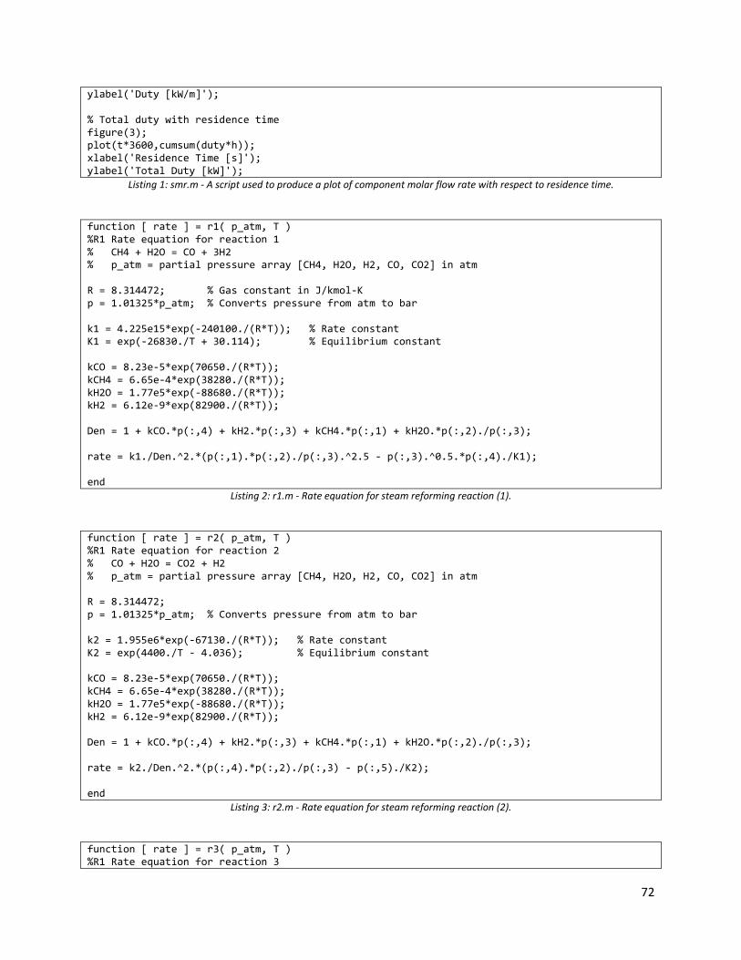
72
ylabel('Duty [kW/m]'); % Total duty with residence time figure(3); plot(t*3600,cumsum(duty*h)); xlabel('Residence Time [s]'); ylabel('Total Duty [kW]');
Listing 1: smr.m - A script used to produce a plot of component molar flow rate with respect to residence time.
function [ rate ] = r1( p_atm, T ) %R1 Rate equation for reaction 1 % CH4 + H2O = CO + 3H2 % p_atm = partial pressure array [CH4, H2O, H2, CO, CO2] in atm R = 8.314472; % Gas constant in J/kmol-K p = 1.01325*p_atm; % Converts pressure from atm to bar k1 = 4.225e15*exp(-240100./(R*T)); % Rate constant K1 = exp(-26830./T + 30.114); % Equilibrium constant kCO = 8.23e-5*exp(70650./(R*T)); kCH4 = 6.65e-4*exp(38280./(R*T)); kH2O = 1.77e5*exp(-88680./(R*T)); kH2 = 6.12e-9*exp(82900./(R*T)); Den = 1 + kCO.*p(:,4) + kH2.*p(:,3) + kCH4.*p(:,1) + kH2O.*p(:,2)./p(:,3); rate = k1./Den.^2.*(p(:,1).*p(:,2)./p(:,3).^2.5 - p(:,3).^0.5.*p(:,4)./K1); end
Listing 2: r1.m - Rate equation for steam reforming reaction (1).
function [ rate ] = r2( p_atm, T ) %R1 Rate equation for reaction 2 % CO + H2O = CO2 + H2 % p_atm = partial pressure array [CH4, H2O, H2, CO, CO2] in atm R = 8.314472; p = 1.01325*p_atm; % Converts pressure from atm to bar k2 = 1.955e6*exp(-67130./(R*T)); % Rate constant K2 = exp(4400./T - 4.036); % Equilibrium constant kCO = 8.23e-5*exp(70650./(R*T)); kCH4 = 6.65e-4*exp(38280./(R*T)); kH2O = 1.77e5*exp(-88680./(R*T)); kH2 = 6.12e-9*exp(82900./(R*T)); Den = 1 + kCO.*p(:,4) + kH2.*p(:,3) + kCH4.*p(:,1) + kH2O.*p(:,2)./p(:,3); rate = k2./Den.^2.*(p(:,4).*p(:,2)./p(:,3) - p(:,5)./K2); end
Listing 3: r2.m - Rate equation for steam reforming reaction (2).
function [ rate ] = r3( p_atm, T ) %R1 Rate equation for reaction 3
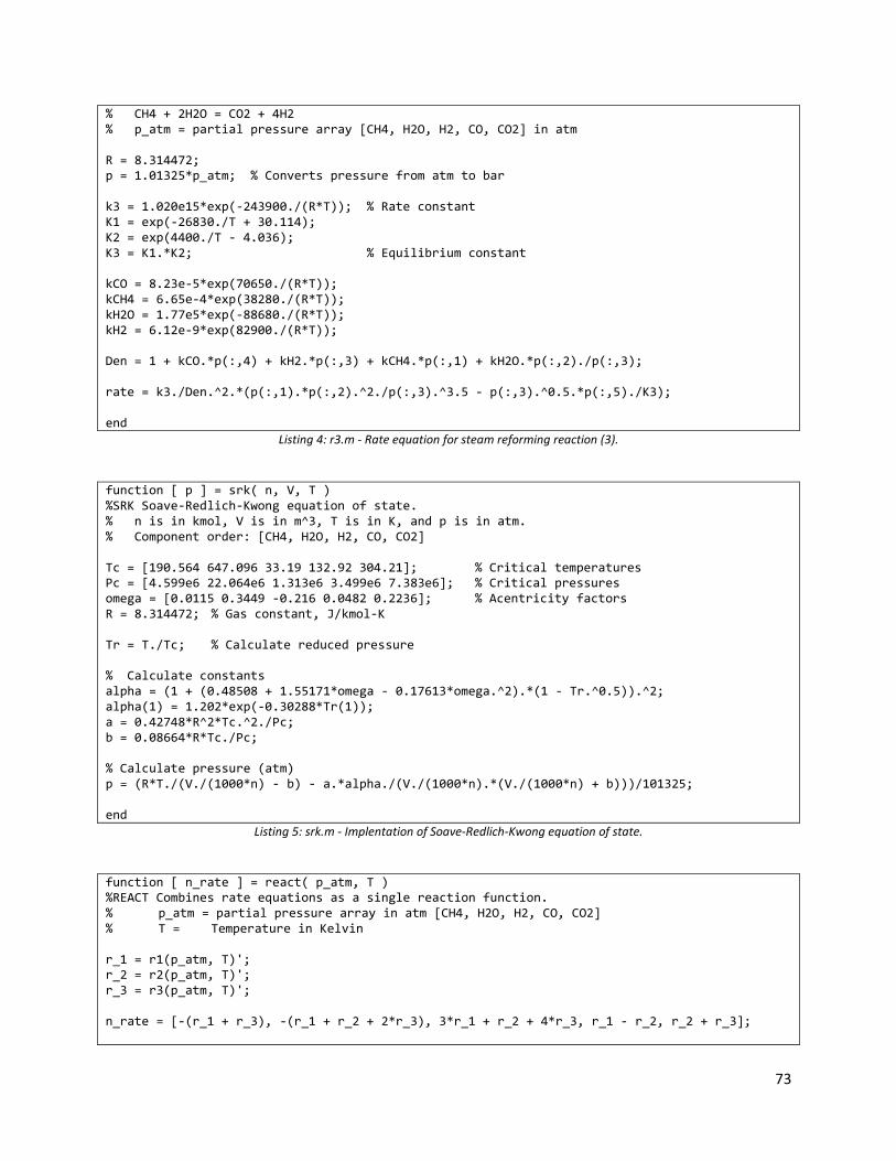
73
% CH4 + 2H2O = CO2 + 4H2 % p_atm = partial pressure array [CH4, H2O, H2, CO, CO2] in atm R = 8.314472; p = 1.01325*p_atm; % Converts pressure from atm to bar k3 = 1.020e15*exp(-243900./(R*T)); % Rate constant K1 = exp(-26830./T + 30.114); K2 = exp(4400./T - 4.036); K3 = K1.*K2; % Equilibrium constant kCO = 8.23e-5*exp(70650./(R*T)); kCH4 = 6.65e-4*exp(38280./(R*T)); kH2O = 1.77e5*exp(-88680./(R*T)); kH2 = 6.12e-9*exp(82900./(R*T)); Den = 1 + kCO.*p(:,4) + kH2.*p(:,3) + kCH4.*p(:,1) + kH2O.*p(:,2)./p(:,3); rate = k3./Den.^2.*(p(:,1).*p(:,2).^2./p(:,3).^3.5 - p(:,3).^0.5.*p(:,5)./K3); end
Listing 4: r3.m - Rate equation for steam reforming reaction (3).
function [ p ] = srk( n, V, T ) %SRK Soave-Redlich-Kwong equation of state. % n is in kmol, V is in m^3, T is in K, and p is in atm. % Component order: [CH4, H2O, H2, CO, CO2] Tc = [190.564 647.096 33.19 132.92 304.21]; % Critical temperatures Pc = [4.599e6 22.064e6 1.313e6 3.499e6 7.383e6]; % Critical pressures omega = [0.0115 0.3449 -0.216 0.0482 0.2236]; % Acentricity factors R = 8.314472; % Gas constant, J/kmol-K Tr = T./Tc; % Calculate reduced pressure % Calculate constants alpha = (1 + (0.48508 + 1.55171*omega - 0.17613*omega.^2).*(1 - Tr.^0.5)).^2; alpha(1) = 1.202*exp(-0.30288*Tr(1)); a = 0.42748*R^2*Tc.^2./Pc; b = 0.08664*R*Tc./Pc; % Calculate pressure (atm) p = (R*T./(V./(1000*n) - b) - a.*alpha./(V./(1000*n).*(V./(1000*n) + b)))/101325; end
Listing 5: srk.m - Implentation of Soave-Redlich-Kwong equation of state.
function [ n_rate ] = react( p_atm, T ) %REACT Combines rate equations as a single reaction function. % p_atm = partial pressure array in atm [CH4, H2O, H2, CO, CO2] % T = Temperature in Kelvin r_1 = r1(p_atm, T)'; r_2 = r2(p_atm, T)'; r_3 = r3(p_atm, T)'; n_rate = [-(r_1 + r_3), -(r_1 + r_2 + 2*r_3), 3*r_1 + r_2 + 4*r_3, r_1 - r_2, r_2 + r_3];
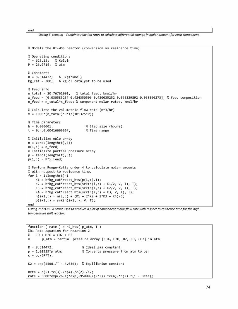
74
end Listing 6: react.m - Combines reaction rates to calculate differential change in molar amount for each component.
% Models the HT-WGS reactor (conversion vs residence time) % Operating conditions T = 623.15; % Kelvin P = 26.9714; % atm % Constants R = 8.314472; % J/(K*kmol) kg_cat = 300; % kg of catalyst to be used % Feed info n_total = 20.76761001; % total feed, kmol/hr x_feed = [0.030585237 0.424350506 0.420035252 0.065329892 0.058360273]; % feed composition n_feed = n_total*x_feed; % component molar rates, kmol/hr % Calculate the volumetric flow rate (m^3/hr) V = 1000*(n_total)*R*T/(101325*P); % Time parameters h = 0.000001; % Step size (hours) t = 0:h:0.00416666667; % Time range % Initialize mole array n = zeros(length(t),5); n(1,:) = n_feed; % Initialize partial pressure array p = zeros(length(t),5); p(1,:) = P*x_feed; % Perform Runge-Kutta order 4 to caluclate molar amounts % with respect to residence time. for i = 1:length(t)-1 K1 = h*kg_cat*react_hts(p(i,:),T); K2 = h*kg_cat*react_hts(srk(n(i,:) + K1/2, V, T), T); K3 = h*kg_cat*react_hts(srk(n(i,:) + K2/2, V, T), T); K4 = h*kg_cat*react_hts(srk(n(i,:) + K3, V, T), T); n(i+1,:) = n(i,:) + (K1 + 2*K2 + 2*K3 + K4)/6; p(i+1,:) = srk(n(i+1,:), V, T); end Listing 7: hts.m - A script used to produce a plot of component molar flow rate with respect to residence time for the high temperature shift reactor.
function [ rate ] = r2_hts( p_atm, T ) %R1 Rate equation for reaction 2 % CO + H2O = CO2 + H2 % p_atm = partial pressure array [CH4, H2O, H2, CO, CO2] in atm R = 8.314472; % Ideal gas constant p = 1.01325*p_atm; % Converts pressure from atm to bar c = p./(R*T); K2 = exp(4400./T - 4.036); % Equilibrium constant Beta = c(5).*c(3)./c(4)./c(2)./K2; rate = 3600*exp(26.1)*exp(-95000./(R*T)).*c(4).*c(2).*(1 - Beta);
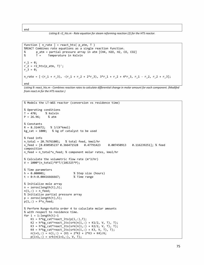
75
end
Listing 8: r2_hts.m - Rate equation for steam reforming reaction (2) for the HTS reactor.
function [ n_rate ] = react_hts( p_atm, T ) %REACT Combines rate equations as a single reaction function. % p_atm = partial pressure array in atm [CH4, H2O, H2, CO, CO2] % T = Temperature in Kelvin r_1 = 0; r_2 = r2_hts(p_atm, T)'; r_3 = 0; n_rate = [-(r_1 + r_3), -(r_1 + r_2 + 2*r_3), 3*r_1 + r_2 + 4*r_3, r_1 - r_2, r_2 + r_3]; end Listing 9: react_hts.m - Combines reaction rates to calculate differential change in molar amount for each component. (Modifed from react.m for the HTS reactor.)
% Models the LT-WGS reactor (conversion vs residence time) % Operating conditions T = 470; % Kelvin P = 26.96; % atm % Constants R = 8.314472; % J/(K*kmol) kg_cat = 1000; % kg of catalyst to be used % Feed info n_total = 20.76761001; % total feed, kmol/hr x_feed = [0.030585237 0.366471528 0.47791423 0.007450913 0.116239251]; % feed composition n_feed = n_total*x_feed; % component molar rates, kmol/hr % Calculate the volumetric flow rate (m^3/hr) V = 1000*(n_total)*R*T/(101325*P); % Time parameters h = 0.000001; % Step size (hours) t = 0:h:0.00416666667; % Time range % Initialize mole array n = zeros(length(t),5); n(1,:) = n_feed; % Initialize partial pressure array p = zeros(length(t),5); p(1,:) = P*x_feed; % Perform Runge-Kutta order 4 to caluclate molar amounts % with respect to residence time. for i = 1:length(t)-1 K1 = h*kg_cat*react_lts(p(i,:),T); K2 = h*kg_cat*react_lts(srk(n(i,:) + K1/2, V, T), T); K3 = h*kg_cat*react_lts(srk(n(i,:) + K2/2, V, T), T); K4 = h*kg_cat*react_lts(srk(n(i,:) + K3, V, T), T); n(i+1,:) = n(i,:) + (K1 + 2*K2 + 2*K3 + K4)/6; p(i+1,:) = srk(n(i+1,:), V, T);
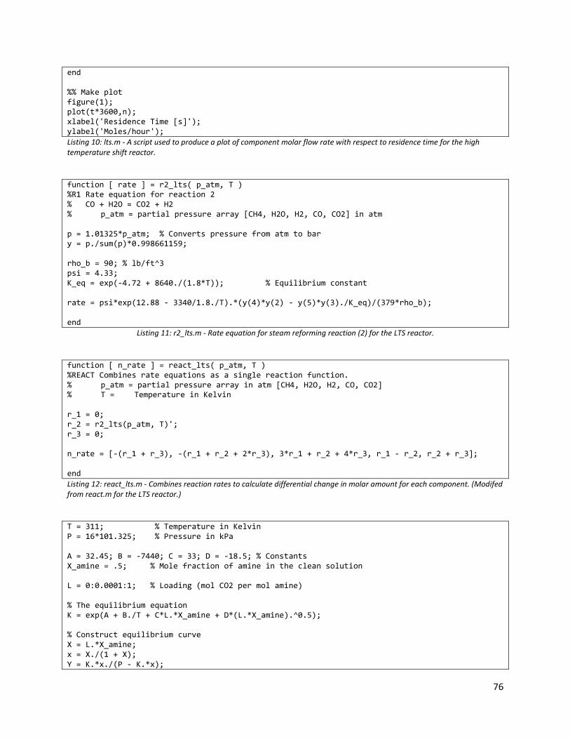
76
end %% Make plot figure(1); plot(t*3600,n); xlabel('Residence Time [s]'); ylabel('Moles/hour'); Listing 10: lts.m - A script used to produce a plot of component molar flow rate with respect to residence time for the high temperature shift reactor.
function [ rate ] = r2_lts( p_atm, T ) %R1 Rate equation for reaction 2 % CO + H2O = CO2 + H2 % p_atm = partial pressure array [CH4, H2O, H2, CO, CO2] in atm p = 1.01325*p_atm; % Converts pressure from atm to bar y = p./sum(p)*0.998661159; rho_b = 90; % lb/ft^3 psi = 4.33; K_eq = exp(-4.72 + 8640./(1.8*T)); % Equilibrium constant rate = psi*exp(12.88 - 3340/1.8./T).*(y(4)*y(2) - y(5)*y(3)./K_eq)/(379*rho_b); end
Listing 11: r2_lts.m - Rate equation for steam reforming reaction (2) for the LTS reactor.
function [ n_rate ] = react_lts( p_atm, T ) %REACT Combines rate equations as a single reaction function. % p_atm = partial pressure array in atm [CH4, H2O, H2, CO, CO2] % T = Temperature in Kelvin r_1 = 0; r_2 = r2_lts(p_atm, T)'; r_3 = 0; n_rate = [-(r_1 + r_3), -(r_1 + r_2 + 2*r_3), 3*r_1 + r_2 + 4*r_3, r_1 - r_2, r_2 + r_3]; end Listing 12: react_lts.m - Combines reaction rates to calculate differential change in molar amount for each component. (Modifed from react.m for the LTS reactor.)
T = 311; % Temperature in Kelvin P = 16*101.325; % Pressure in kPa A = 32.45; B = -7440; C = 33; D = -18.5; % Constants X_amine = .5; % Mole fraction of amine in the clean solution L = 0:0.0001:1; % Loading (mol CO2 per mol amine) % The equilibrium equation K = exp(A + B./T + C*L.*X_amine + D*(L.*X_amine).^0.5); % Construct equilibrium curve X = L.*X_amine; x = X./(1 + X); Y = K.*x./(P - K.*x);
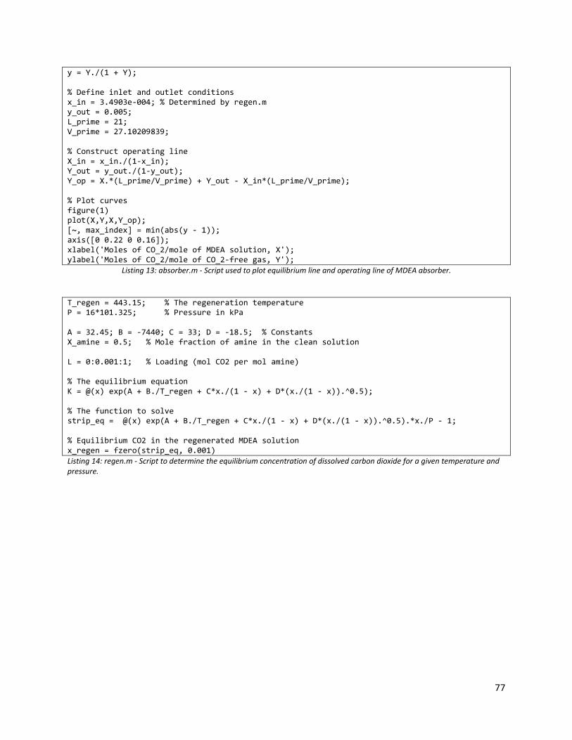
77
y = Y./(1 + Y); % Define inlet and outlet conditions x_in = 3.4903e-004; % Determined by regen.m y_out = 0.005; L_prime = 21; V_prime = 27.10209839; % Construct operating line X_in = x_in./(1-x_in); Y_out = y_out./(1-y_out); Y_op = X.*(L_prime/V_prime) + Y_out - X_in*(L_prime/V_prime); % Plot curves figure(1) plot(X,Y,X,Y_op); [~, max_index] = min(abs(y - 1)); axis([0 0.22 0 0.16]); xlabel('Moles of CO_2/mole of MDEA solution, X'); ylabel('Moles of CO_2/mole of CO_2-free gas, Y');
Listing 13: absorber.m - Script used to plot equilibrium line and operating line of MDEA absorber.
T_regen = 443.15; % The regeneration temperature P = 16*101.325; % Pressure in kPa A = 32.45; B = -7440; C = 33; D = -18.5; % Constants X_amine = 0.5; % Mole fraction of amine in the clean solution L = 0:0.001:1; % Loading (mol CO2 per mol amine) % The equilibrium equation K = @(x) exp(A + B./T_regen + C*x./(1 - x) + D*(x./(1 - x)).^0.5); % The function to solve strip_eq = @(x) exp(A + B./T_regen + C*x./(1 - x) + D*(x./(1 - x)).^0.5).*x./P - 1; % Equilibrium CO2 in the regenerated MDEA solution x_regen = fzero(strip_eq, 0.001) Listing 14: regen.m - Script to determine the equilibrium concentration of dissolved carbon dioxide for a given temperature and pressure.


