61
Milan, 24 th October 2017 Hydrogeological issues in geological hazard assessment Paola Gattinoni Research area: Transport Infrastructure and Geosciences

Milan, 24th October 2017
Hydrogeological issues in geological hazard assessment
Paola GattinoniResearch area: Transport Infrastructure and Geosciences

• Groundwater resources depletion
• Landslides and river dynamic
• Civil constructions (i.e. tunnels, roads)
GEOLOGICAL HAZARDS
HYDROGEOLOGICAL CONCEPTUAL MODEL
Main research topics ⇒ Engineering Geology

1. Type of aquifer ⇐ geomaterials
2. Hydraulic conductivity
3. Groundwater level
4. Hydrogeological balance
Which issues are involved in the reconstruction of the hydrogeological conceptual model ?
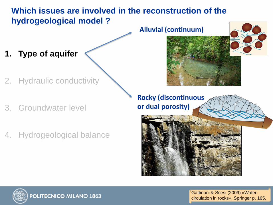
1. Type of aquifer
2. Hydraulic conductivity
3. Groundwater level
4. Hydrogeological balance
Which issues are involved in the reconstruction of the hydrogeological model ?
Alluvial (continuum)
Rocky (discontinuous or dual porosity)
Gattinoni & Scesi (2009) «Water circulation in rocks», Springer p. 165.
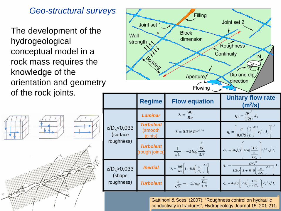
The development of the hydrogeological conceptual model in a rock mass requires the knowledge of the orientation and geometry of the rock joints.
Geo-structural surveys
Gattinoni & Scesi (2007): “Roughness control on hydraulic conductivity in fractures”, Hydrogeology Journal 15: 201-211.
Regime Flow equation Unitary flow rate (m2/s)
ε/Dh<0,033(surface
roughness)
Laminar
Turbolent(smooth joints)
Turbolent(rough joints)
ε/Dh>0,033(shape
roughness)
Inertial
Turbolent
Re96
=λi
ii J
geq
υ12
3
=
413160 /Re. −=λ
7/4
34/12
079.0
⋅
= iii Jegqυ
7321
.Dlog h
ε
−=λ
ii
h
i Je
D
gq 5.17.3log4
= ε
ε+=λ
51
88196.
hD.
Re
i
h
ii J
D
geq
+
=5.1
3
8.8112 ευ
9121
.Dlog h
ε
−=λ
iih
i JeD
gq 5.1
/9.1log4
=
ε
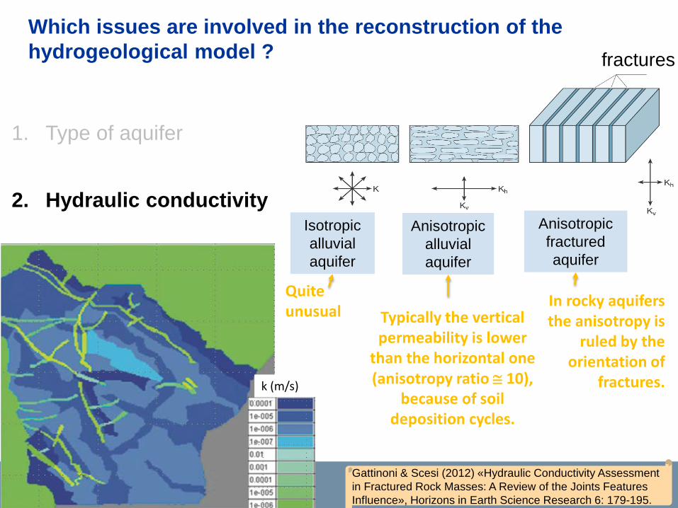
Anisotropicalluvialaquifer
Anisotropicfracturedaquifer
Isotropicalluvialaquifer
fractures
Quite unusual Typically the vertical
permeability is lower than the horizontal one (anisotropy ratio ≅ 10),
because of soil deposition cycles.
In rocky aquifers the anisotropy is
ruled by the orientation of
fractures.
1. Type of aquifer
2. Hydraulic conductivity
3. Groundwater level
4. Hydrogeological balance
Which issues are involved in the reconstruction of the hydrogeological model ?
Gattinoni & Scesi (2012) «Hydraulic Conductivity Assessment in Fractured Rock Masses: A Review of the Joints Features Influence», Horizons in Earth Science Research 6: 179-195.
k (m/s)
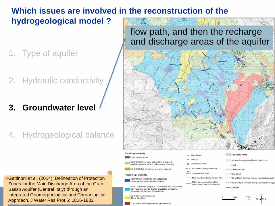
1. Type of aquifer
2. Hydraulic conductivity
3. Groundwater level
4. Hydrogeological balance
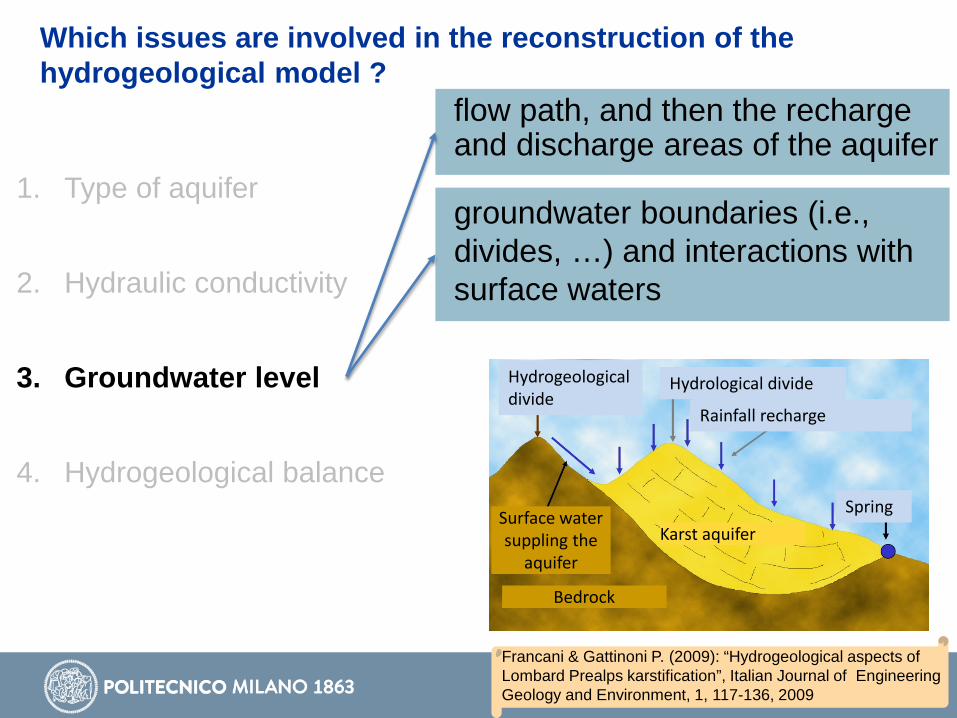
Which issues are involved in the reconstruction of the hydrogeological model ?
flow path, and then the recharge and discharge areas of the aquifer
Gattinoni et al. (2014): Delineation of Protection Zones for the Main Discharge Area of the Gran Sasso Aquifer (Central Italy) through an Integrated Geomorphological and Chronological Approach, J Water Res Prot 6: 1816-1832.
1. Type of aquifer
2. Hydraulic conductivity
3. Groundwater level
4. Hydrogeological balance
Which issues are involved in the reconstruction of the hydrogeological model ?
groundwater boundaries (i.e., divides, …) and interactions with surface waters
flow path, and then the recharge and discharge areas of the aquifer
Hydrological divide
Rainfall recharge
Spring
Hydrogeological divide
Surface water suppling the
aquifer
Bedrock
Karst aquifer
Francani & Gattinoni P. (2009): “Hydrogeological aspects of Lombard Prealps karstification”, Italian Journal of Engineering Geology and Environment, 1, 117-136, 2009

1. Type of aquifer
2. Hydraulic conductivity
3. Groundwater level
4. Hydrogeological balance
Which issues are involved in the reconstruction of the hydrogeological model ?
water table changes in time
groundwater boundaries (i.e., divides, …) and interactions with surface waters
flow path, and then the recharge and discharge areas of the aquifer
1970 1996Gattinoni et al (2003): “Pumping from quarry lakes as a measure for groundwater control in Milan: efficacy, feasability and hydrogeological constrains” – Appl Geol J 10(1): 33-46.

1. Type of aquifer
2. Hydraulic conductivity
3. Groundwater level
4. Hydrogeological balance
Which issues are involved in the reconstruction of the hydrogeological model ?
Fracture zone → connected aquifers
Shallow aquifer
Deep aquifer
i
hdhs
ht
hdSprings
Tunnel
Recharge
Deep aquiferhr qupRivers
Shallowaquifer
Gattinoni & Scesi (2006): Hydrogeological hazard assessment in medium depth tunnels, J Appl Geol 79: 69-79.
dstundownupd
dss
qqqqt
V
qit
V
−
−
+−−=∆∆
−=∆∆
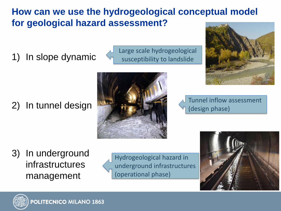
1) In slope dynamic
2) In tunnel design
3) In underground infrastructures management
How can we use the hydrogeological conceptual model for geological hazard assessment?
Large scale hydrogeological susceptibility to landslide
Tunnel inflow assessment (design phase)
Hydrogeological hazard in underground infrastructures (operational phase)

A lesson we learnedStructural and
lithological setting
Hydrogeological setting
Hydrometric level of the lake which could trigger the landslide even without rainfall.
Rainfall which could trigger the landslide even without the lake.Collapse
Gattinoni et al. (2005): “Dynamic conceptual models for risk assessment in design”, J Appl Geol 12: 35-47.
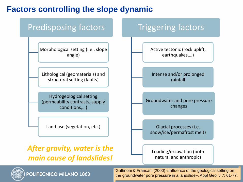
Factors controlling the slope dynamic
Predisposing factors
Morphological setting (i.e., slope angle)
Lithological (geomaterials) and structural setting (faults)
Hydrogeological setting (permeability contrasts, supply
conditions,…)
Land use (vegetation, etc.)
Triggering factors
Active tectonic (rock uplift, earthquakes,…)
Intense and/or prolonged rainfall
Groundwater and pore pressure changes
Glacial processes (i.e. snow/ice/permafrost melt)
Loading/excavation (both natural and anthropic)
After gravity, water is the main cause of landslides!
Gattinoni & Francani (2000) «Influence of the geological setting on the groundwater pore pressure in a landslide», Appl Geol J 7: 61-77.
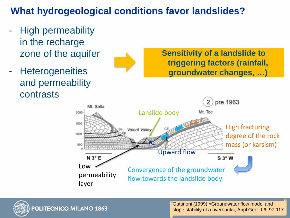
High fracturing degree of the rock mass (or karsism)
What hydrogeological conditions favor landslides?
Gattinoni (1999) «Groundwater flow model and slope stability of a riverbank», Appl Geol J 6: 97-117.
- High permeability in the recharge zone of the aquifer
- Heterogeneities and permeability contrasts
Upward flow
Convergence of the groundwater flow towards the landslide body
Lanslide body
Low permeability layer
Sensitivity of a landslide to triggering factors (rainfall, groundwater changes, …)
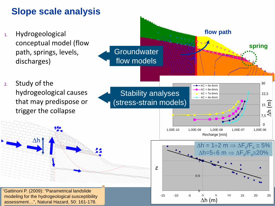
1. Hydrogeological conceptual model (flow path, springs, levels, discharges)
2. Study of the hydrogeological causes that may predispose or trigger the collapse
y = -0.0267x + 1R2 = 0.8122
0
0.5
1
1.5
-15 -10 -5 0 5 10 15 20 25
Dh nel detrito [m]
Fs
Slope scale analysis
flow path
spring
∆h
∆h (m)
Gattinoni P. (2009): “Parametrical landslide modeling for the hydrogeological susceptibility assessment…”, Natural Hazard, 50: 161-178.
Groundwaterflow models
1,00E-10 1,00E-09 1,00E-08 1,00E-07 1,00E-06Recharge [m/s]
kC = 5e-6m/skC = 6e-6m/skC = 7e-6m/skC = 4e-6m/s
Stability analyses (stress-strain models)
∆h = 1÷2 m ⇒ ∆Fs/Fs ≅ 5%∆h=5÷6 m ⇒ ∆Fs/Fs≅20%
∆h (m
)
0
30
15
7,5
22,5
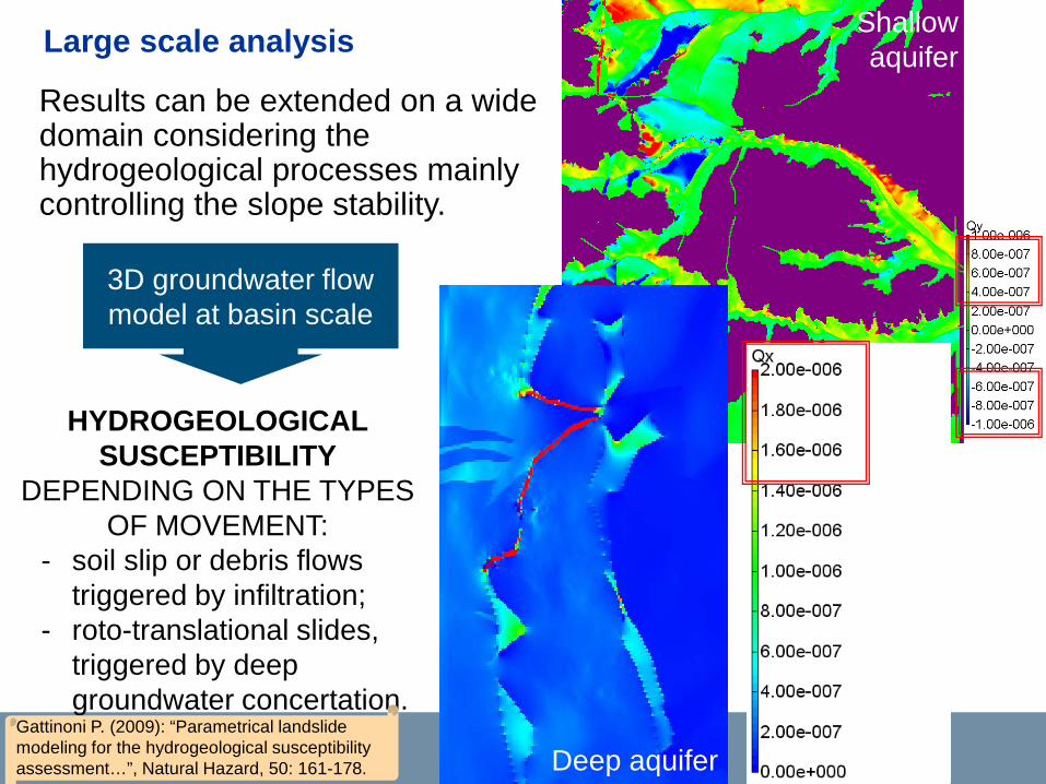
Large scale analysis
Results can be extended on a wide domain considering the hydrogeological processes mainly controlling the slope stability.
3D groundwater flow model at basin scale
HYDROGEOLOGICAL SUSCEPTIBILITY
DEPENDING ON THE TYPES OF MOVEMENT:
- soil slip or debris flows triggered by infiltration;
- roto-translational slides, triggered by deep groundwater concertation.
Shallowaquifer
Deep aquiferGattinoni P. (2009): “Parametrical landslide modeling for the hydrogeological susceptibility assessment…”, Natural Hazard, 50: 161-178.
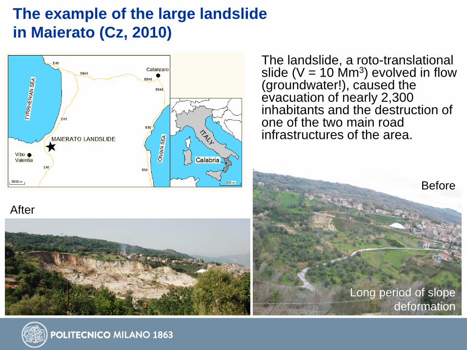
The landslide, a roto-translational slide (V = 10 Mm3) evolved in flow (groundwater!), caused the evacuation of nearly 2,300 inhabitants and the destruction of one of the two main road infrastructures of the area.
The example of the large landslidein Maierato (Cz, 2010)
Before
After
Long period of slope deformation
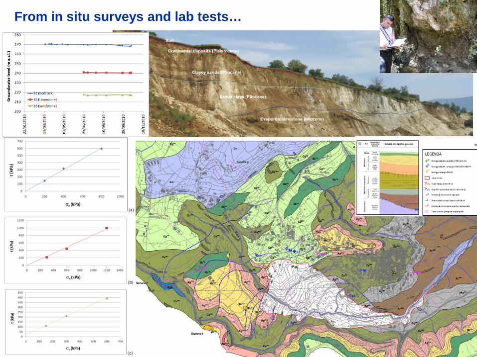
From in situ surveys and lab tests…

…to the landslide conceptual model…
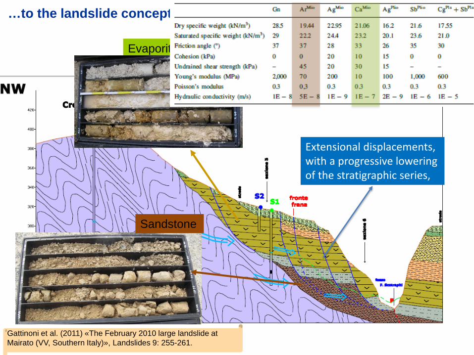
Gattinoni et al. (2011) «The February 2010 large landslide atMairato (VV, Southern Italy)», Landslides 9: 255-261.
Evaporitic limestone
Sandstone
Claystone
Drillings ⇒ geological weakness of the geomaterials
Weak rocks for lithology (very high primary porosity, behavior from plastic to quasi-liquid depending on the water content)
Weak rocks for weathering (almost no cement)
…to the landslide conceptual model…
Gattinoni et al. (2011) «The February 2010 large landslide atMairato (VV, Southern Italy)», Landslides 9: 255-261.
Evaporitic limestone
Sandstone
Extensional displacements, with a progressive lowering of the stratigraphic series,

…to the landslide conceptual model…
Gattinoni et al. (2011) «The February 2010 large landslide atMairato (VV, Southern Italy)», Landslides 9: 255-261.
Limestone
Sandstone
ClaystonePhylliticbedrock

…to the landslide conceptual model…
Gattinoni et al. (2011) «The February 2010 large landslide atMairato (VV, Southern Italy)», Landslides 9: 255-261.
Phylliticbedrock
Evaporiticlimestone
Sandstone
Claystone
RainfalI in the last 20 days before the collapse: 100-years return period
Max monthly rainfall of the last 60 years (ARPACAL, 2010).

H[m a.s.l.]
FSDrained cond.
FSUndrained cond
269.8 1.30 1.25273.7 1.25 1.20275.1 1.20 1.15283.5 1.05 1.00
Simulations were carried out by changing thegroundwater level in order to point out the criticalconditions, corresponding to an increase of thewater table of about 15 m.
From the conceptual to the 2D numerical model
Groundwater
Shear stress increment
Displacement

Similar geological and hydrogeological conditions in the whole urban area!
Is there a residual risk?
What’s the hazard in the urban area?
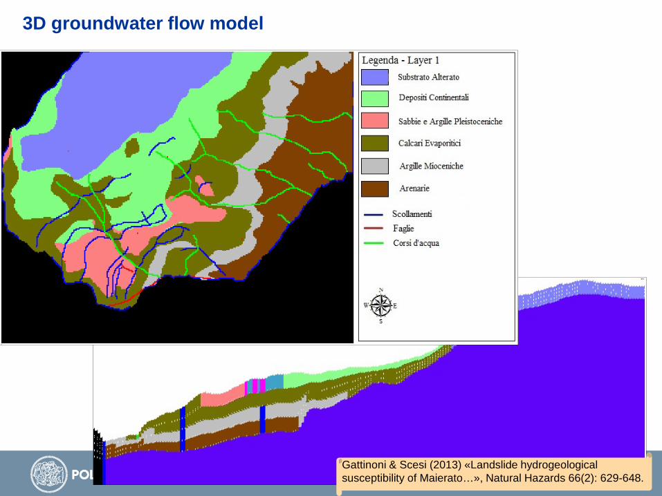
3D groundwater flow model
Gattinoni & Scesi (2013) «Landslide hydrogeologicalsusceptibility of Maierato…», Natural Hazards 66(2): 629-648.
180
200
220
240
260
280
300
320
180 200 220 240 260 280 300 320
Simulated
Observed
Layer 1
Layer 2
Layer 3
Layer 4
Layer 5
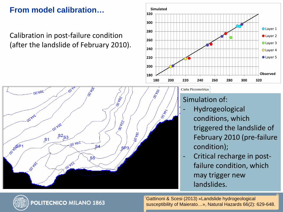
From model calibration…
Calibration in post-failure condition (after the landslide of February 2010).
Simulation of: - Hydrogeological
conditions, which triggered the landslide of February 2010 (pre-failure condition);
- Critical recharge in post-failure condition, which may trigger new landslides.
Gattinoni & Scesi (2013) «Landslide hydrogeologicalsusceptibility of Maierato…», Natural Hazards 66(2): 629-648.

…to the hydrogeological susceptibility assessment
Groundwater flow rates
Water table drawdowns
Gattinoni & Scesi (2013) «Landslide hydrogeologicalsusceptibility of Maierato…», Natural Hazards 66(2): 629-648.
Zones interested by groundwater flow
concentration

1) In slope dynamic
2) In tunnel design
3) In underground infrastructures management
How can we use the hydrogeological conceptual model for geological hazard assessment?
Large scale hydrogeological susceptibility to landslide
Tunnel inflow assessment (design phase)
Hydrogeological hazard in underground infrastructures (operational phase)

Geological hazards in tunneling
Hazards for the tunnel Hazards for the environment
- Tunnel and face instability or
deformation
- Water inflow
- Gas and aggressive waters
- Water resources pollution
- Drying up or changes in spring regime
- Water table drawdown
- Surface settlements
- Landslides
Hydrogeological issues are involved in both the points of view…
Draining tunnel
Zone with springs influenced by water table drawdown
Initial water tableFinal water table
Water management and delivery system
Gattinoni et al. (2014): Engineering Geology for Underground Works, Springer, p. 305.

- High permeability geomaterials (i.e., granular soils, karst phenomena, porous or fractured rocks)
- Morphological setting (i.e. shallow tunnel, portals)
- Permeability contrast, buried river beds
- Faults or overtrhustshaving significant water supply, synclinal folds
Hydrogeological conditions which could lead to significant water inflow in tunnel:
River
SpringDetriticalcover
Fractured rock
Moraine
Tunnel
Paleochannel
Sandstones
Limestones
GranitesTunnel
Gattinoni et al. (2014): Engineering Geology for Underground Works, Springer, p. 305.
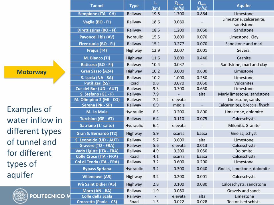
Tunnel Type L.(km)
Qmax(m³/s)
Qmin(m³/s) Aquifer
Sempione (ITA - CH) Railway 19.8 1.700 0.864 Limestone
Vaglia (BO - FI) Railway 18.6 0.080 - Limestone, calcarenite, sandstone
Direttissima (BO - FI) Railway 18.5 1.200 0.060 SandstonePavoncelli bis (AV) Hydraulic 15.5 0.800 0.070 Limestone, Clay Firenzuola (BO - FI) Railway 15.1 0.277 0.070 Sandstone and marl
Frejus (T4) Highway 12.9 0.007 0.001 Several
M. Bianco (Ti) Highway 11.6 0.800 0.440 Granite Raticosa (BO - FI) Railway 10.4 0.037 - Sandstone, marl and clayGran Sasso (A24) Highway 10.2 3.000 0.600 LimestoneS. Lucia (NA - SA) Railway 10.2 1.000 0.250 Limestone
Putifigari (SS) Road 9.8 0.070 0.050 VulcanitesZuc del Bor (UD - AUT) Railway 9.3 0.700 0.650 Limestone
S. Stefano (GE - F) Railway 7.9 - alta Marly limestone, sandstoneM. Olimpino 2 (MI - CO) Railway 7.2 elevata - Limestone, sands
Serena (PR - SP) Railway 6.9 media - Calcarenites, breccia, flyschM. La Mula Hydraulic 6.3 0.200 0.800 Limestone, dolomite
Turchino (GE - AT) Railway 6.4 0.110 0.075 CalceschystsSatriano (1° salto) Hydraulic 6.4 elevata - Milonitic Granite
Gran S. Bernardo (T2) Highway 5.9 scarsa bassa Gneiss, schystS. Leopoldo (UD - AUT) Railway 5.7 3.600 alta Limestone
Gravere (TO - FRA) Railway 5.6 elevata 0.013 CalceschystsVado Ligure (ITA - FRA) Railway 4.9 0.200 0.050 DolomiteColle Croce (ITA - FRA) Road 4.1 scarsa bassa CalceschystsCol di Tenda (ITA - FRA) Railway 3.2 0.600 0.200 Limestone
Bypass Spriana Hydraulic 3.2 0.300 0.040 Gneiss, limestone, dolomite
Villeneuve (A5) Highway 3.2 0.200 0.001 Calceschysts
Prè Saint Didier (A5) Highway 2.8 0.100 0.080 Calceschysts, sandstoneMoro (AN - BA) Railway 1.9 0.080 - Gravels and sandsColle della Scala Railway - elevata alta Limestone
Croccetta (Paola - CS) Road 1.5 0.022 0.028 Tectonised schists
Motorway
Examples of water inflow in different types of tunnel and for different types of aquifer
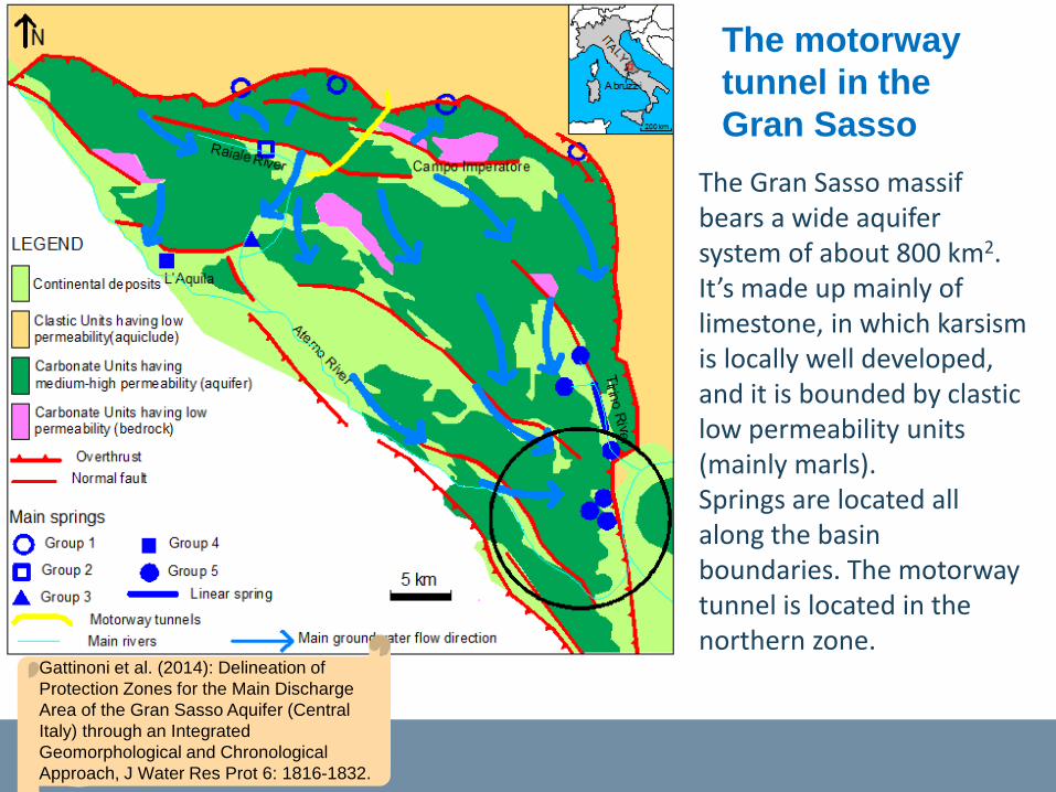
The motorwaytunnel in the Gran Sasso
The Gran Sasso massifbears a wide aquifer system of about 800 km2. It’s made up mainly of limestone, in which karsismis locally well developed, and it is bounded by clastic low permeability units (mainly marls).Springs are located all along the basin boundaries. The motorway tunnel is located in the northern zone.
Gattinoni et al. (2014): Delineation of Protection Zones for the Main Discharge Area of the Gran Sasso Aquifer (Central Italy) through an Integrated Geomorphological and Chronological Approach, J Water Res Prot 6: 1816-1832.
Ricarica:
> 1000 mm/anno
500-1000 mm/anno
250-500 mm/anno
< 250 mm/anno
Sorgenti principali
Sorgente lineare
Drenaggio tunnel autostradale
SovrascorrimentoFaglia distensiva
Direzione di flusso ipogeo principale
T2
Campo Imperatore
Gruppo 1
Gruppo 2
Gruppo 3
Gruppo 4
Gruppo 5
L'Aquila
F. Raiale
Fiumi principali
F. Aterno
F. Tirino
N
5 km
Area di cava prevista
0
1000
2000
ms.l.m.
0
1000
2000
ms.l.m.
NO SE
LEGENDA
CampoImperatore
AcquiferoAquicludeSovrascorrimentoLivello piezometrico indicativo
Direzione di flusso dell'acquiferoInfiltrazione concentrataGruppo sorgivoOpere in sotterraneo
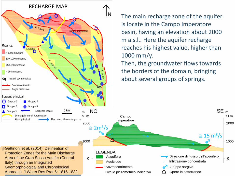
RECHARGE MAP
The main recharge zone of the aquifer is locate in the Campo Imperatorebasin, having an elevation about 2000 m a.s.l.. Here the aquifer recharge reaches his highest value, higher than 1000 mm/y. Then, the groundwater flows towards the borders of the domain, bringing about several groups of springs.
≅ 15 m3/s≅ 2m3/s
Gattinoni et al. (2014): Delineation of Protection Zones for the Main Discharge Area of the Gran Sasso Aquifer (Central Italy) through an Integrated Geomorphological and Chronological Approach, J Water Res Prot 6: 1816-1832.

The motorway tunnel is locate at the bottom of the aquifer and nowadays it drains about 1,5m3/s, which corresponds to less than 10% of the whole aquifer discharge.
≅ 1.5 m3/s
0
1000
2000
ms.l.m.
0
1000
2000
ms.l.m.
NO SE
LEGENDA
CampoImperatore
AcquiferoAquicludeSovrascorrimentoLivello piezometrico indicativo
Direzione di flusso dell'acquiferoInfiltrazione concentrataGruppo sorgivoOpere in sotterraneo
≅ 15 m3/s≅ 2m3/s
Southern springs
Northern springs
Gattinoni et al. (2014): Delineation of Protection Zones for the Main Discharge Area of the Gran Sasso Aquifer (Central Italy) through an Integrated Geomorphological and Chronological Approach, J Water Res Prot 6: 1816-1832.

Hydrogeological conceptual model
Excavation and tunnel support system that minimise tunnel inflow its interferences with springs and wells
Gattinoni et al. (2014): Engineering Geology for Underground Works, Springer, p.305.
Tunnel design
Expensive geognostic surveys (geophysical surveys, drillings, in bore-hole tests)
Hydr
ogeo
logi
cal r
isk (%
)
Cost
of t
he g
eogn
ostic
surv
eys
Hydrogeological data acquisition (%)
Limit in data acquisition
Best solution
Risk
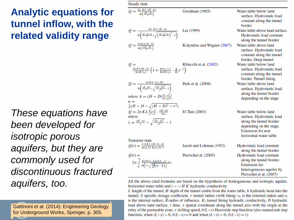
These equations have been developed for isotropic porous aquifers, but they are commonly used for discontinuous fractured aquifers, too.
Analytic equations for tunnel inflow, with the related validity range
Gattinoni et al. (2014): Engineering Geology for Underground Works, Springer, p. 305.
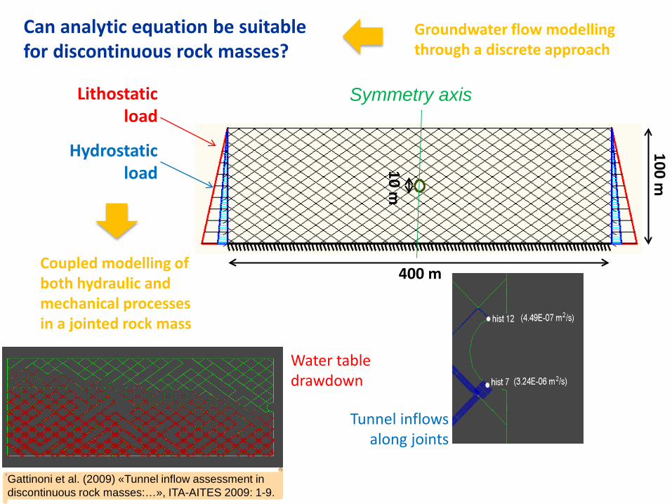
Can analytic equation be suitable for discontinuous rock masses?
400 m
100 m
10 m
Symmetry axis
Groundwater flow modelling through a discrete approach
Coupled modelling of both hydraulic and mechanical processes in a jointed rock mass
Lithostaticload
Hydrostaticload
Water tabledrawdown
Tunnel inflows along joints
Gattinoni et al. (2009) «Tunnel inflow assessment in discontinuous rock masses:…», ITA-AITES 2009: 1-9.
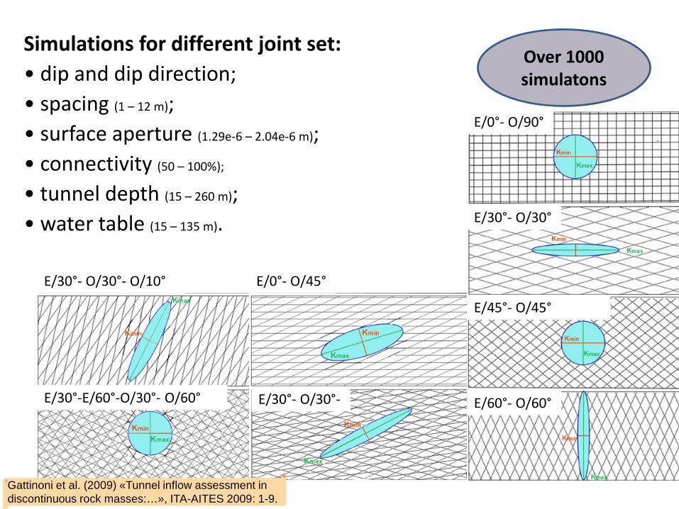
Simulations for different joint set:• dip and dip direction;• spacing (1 – 12 m);• surface aperture (1.29e-6 – 2.04e-6 m);• connectivity (50 – 100%);
• tunnel depth (15 – 260 m);• water table (15 – 135 m).
Over 1000 simulatons
E/45°- O/45°
E/30°- O/30°- O/10° E/0°- O/45°
E/60°- O/60°
E/0°- O/90°
E/30°- O/30°
E/30°- O/30°-E/30°-E/60°-O/30°- O/60°
Gattinoni et al. (2009) «Tunnel inflow assessment in discontinuous rock masses:…», ITA-AITES 2009: 1-9.
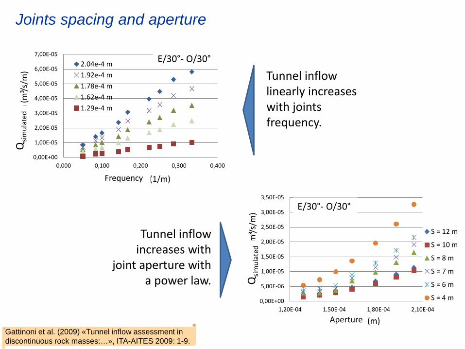
Joints spacing and aperture
0,00E+00
5,00E-06
1,00E-05
1,50E-05
2,00E-05
2,50E-05
3,00E-05
3,50E-05
1,20E-04 1,50E-04 1,80E-04 2,10E-04
Q si
mul
ata
(m³/s
/m)
Apertura (m)
S = 12 m
S = 10 m
S = 8 m
S = 7 m
S = 6 m
S = 4 m
Tunnel inflow linearly increases with joints frequency.
Tunnel inflow increases with
joint aperture with a power law.
0,00E+00
1,00E-05
2,00E-05
3,00E-05
4,00E-05
5,00E-05
6,00E-05
7,00E-05
0,000 0,100 0,200 0,300 0,400
Q si
mul
ata
(m³/s
/m)
Frequenza (1/m)
2.04e-4 m1.92e-4 m1.78e-4 m1.62e-4 m1.29e-4 m
E/30°- O/30°
E/30°- O/30°
Qsim
ulat
ed
Frequency
Qsim
ulat
ed
ApertureGattinoni et al. (2009) «Tunnel inflow assessment in discontinuous rock masses:…», ITA-AITES 2009: 1-9.
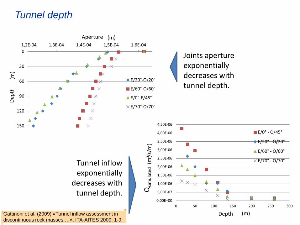
Tunnel depth
0
30
60
90
120
150
1,2E-04 1,3E-04 1,4E-04 1,5E-04 1,6E-04
Prof
ondi
tà(m
)
Aperuta idraulica (m)
E/20°-O/20°
E/60°-O/60°
E/0°-E/45°
E/70°-O/70°
0,00E+00
5,00E-07
1,00E-06
1,50E-06
2,00E-06
2,50E-06
3,00E-06
3,50E-06
4,00E-06
4,50E-06
0 50 100 150 200 250 300
Q si
mul
ata
(m³/s
/m)
Profondità (m)
E/0° - O/45°
E/20° - O/20°
E/60° - O/60°
E/70° - O/70°
Joints aperture exponentially decreases with tunnel depth.
Tunnel inflow exponentially
decreases with tunnel depth. Q
simul
ated
Depth
Dept
h
Aperture
Gattinoni et al. (2009) «Tunnel inflow assessment in discontinuous rock masses:…», ITA-AITES 2009: 1-9.

0,00E+00
1,00E-06
2,00E-06
3,00E-06
4,00E-06
5,00E-06
6,00E-06
7,00E-06
8,00E-06
9,00E-06
0 20 40 60 80 100
Q si
mul
ata
(m³/s
/m)
Inclinazione (°)
Joints dip
0,00E+00
1,00E-05
2,00E-05
3,00E-05
4,00E-05
5,00E-05
6,00E-05
0,0E+00 1,0E-06 2,0E-06 3,0E-06 4,0E-06Q
sim
ulat
a (m
³/s/m
)
Keq (m/s)
E/90° - E/0°
E/30° - O/30°
E/80° - O/80°Qsim
ulat
ed
Qsim
ulat
ed
For the same value of equivalent permeability, tunnel inflow depends on joint dip.
Joints dip
550 joints intersections
213 joints intersections
Orientation of the permeability tensor
Joints connectivity
Gattinoni et al. (2009) «Tunnel inflow assessment in discontinuous rock masses:…», ITA-AITES 2009: 1-9.

Comparison between analytic formula and numerical results for different joint networks
The comparison points out that the analytic formulas overestimate the tunnel inflows and that the overestimation is bigger for geostructural setting having discontinuities with higher dips.
Gattinoni & Scesi (2010) «An empirical equation for tunnel inflow assessment: application to sedimentaryrock masses», Hydrogeol J 18: 1797-1810.
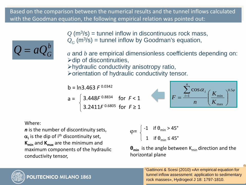
Based on the comparison between the numerical results and the tunnel inflows calculated with the Goodman equation, the following empirical relation was pointed out:
bGaQQ =
Q (m3/s) = tunnel inflow in discontinuous rock mass, QG (m3/s) = tunnel inflow by Goodman’s equation,
a and b are empirical dimensionless coefficients depending on:dip of discontinuities, hydraulic conductivity anisotropy ratio, orientation of hydraulic conductivity tensor.
b = ln3.463 F 0.0342
a = 3.448F 0.8834 for F < 13.2411F 0.6805 for F ≥ 1
ϕα 5.0
max
min1cos
=∑=
KK
nF
n
ii
Where:n is the number of discontinuity sets,αi is the dip of ith discontinuity set,Kmin and Kmax are the minimum and maximum components of the hydraulic conductivity tensor,
ϕ= -1 if θmin > 45°
1 if θmin ≤ 45°
θmin is the angle between Kmin direction and the horizontal plane
Gattinoni & Scesi (2010) «An empirical equation for tunnel inflow assessment: application to sedimentaryrock masses», Hydrogeol J 18: 1797-1810.
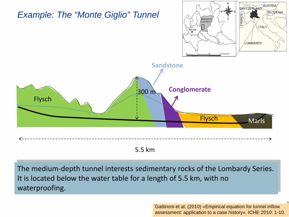
5.5 km
300 m
Example: The “Monte Giglio” Tunnel
Flysch
FlyschConglomerate
Marls
Sandstone
The medium-depth tunnel interests sedimentary rocks of the Lombardy Series.It is located below the water table for a length of 5.5 km, with no waterproofing.
Gattinoni et al. (2010) «Empirical equation for tunnel inflowassessment: application to a case history», ICHE 2010: 1-10.

13 2458 7 6
Flysch
FlyschConglomerate
Marls
Sandstone
The tunnel was divided into hydrogeological homogeneous stretches. For each one, the
hydraulic conductivity tensor and the corresponding equivalent hydraulic
conductivity were calculated based on the structural surveys and on depth pumping
tests, that allowed to consider the decreasing of permeability with depth.
Gattinoni et al. (2010) «Empirical equation for tunnel inflowassessment: application to a case history», ICHE 2010: 1-10.

13 2458 7 6
12345678
In some cases, the hydraulic conductivity ellipses (in the vertical plane orthogonal to the tunnel) show a great anisotropy, with the main hydraulic conductivity parallel to the vertical direction, such as for stretches 2, 4 and 6. As a consequence, for these cases the Goodman equation gives the highest overestimation, whereas the empirical relation allows an estimation of the tunnel inflow that better reproduces the observed values.
0
0,005
0,01
0,015
0,02
0,025
0,03
0,035
12345678
Tunn
el in
flow
[m3 /
s]
Q Goodman Q formula Q observed
Gattinoni et al. (2010) «Empirical equation for tunnel inflowassessment: application to a case history», ICHE 2010: 1-10.

1) In slope dynamic
2) In tunnel design
3) In underground infrastructures management
How can we use the hydrogeological conceptual model for geological hazard assessment?
Large scale hydrogeological susceptibility to landslide
Tunnel inflow assessment (design phase)
Hydrogeological hazard in underground infrastructures (operational phase)
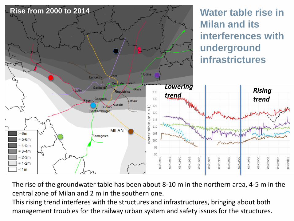
Water table rise in Milan and itsinterferences with underground infrastrictures
The rise of the groundwater table has been about 8-10 m in the northern area, 4-5 m in the central zone of Milan and 2 m in the southern one.This rising trend interferes with the structures and infrastructures, bringing about both management troubles for the railway urban system and safety issues for the structures.
Loweringtrend
Risingtrend
Rise from 2000 to 2014

Examples of interference between groundwater and underground structures and infrastructures
The metro line green, which was designed to function in dry conditions, now lies below the water table, involving important waterproofing works.
If the groundwater trend will go on with the same rate, in the next ten years static problems will be triggered, even in presence of waterproofing lining.

The model domain covers an area with high density of hydrogeological data.
Subsurface geological data (CARG)
Source
DepthBottom surface
Aquifer A
Uppersurface
Aquifer B
Bottom surface
Aquifer BTotal
CARG 1020 731 361 2112
Quite good accuracy in the reconstruction of the aquifer geometry:
Shallow aquifer
Semi-confined aquifer
Aquitard
Gattinoni et al. (2016) «Geological map of Italy– Milan 118», Italian Geological Service.
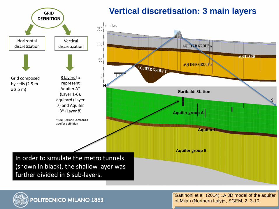
LAYER 2
Horizontaldiscretization
Verticaldiscretization
Grid composedby cells (2,5 m x 2,5 m)
8 layers to representAquifer A* (Layer 1-6),
aquitard (Layer7) and Aquifer
B* (Layer 8)
GRID DEFINITION
* ENI-Regione Lombardia aquifer definition
N
S
Garibaldi Station
Aquifer group B
Aquifer group A
Aquitard
Vertical discretisation: 3 main layers
In order to simulate the metro tunnels (shown in black), the shallow layer was further divided in 6 sub-layers.
Gattinoni et al. (2014) «A 3D model of the aquiferof Milan (Northern Italy)», SGEM, 2: 3-10.
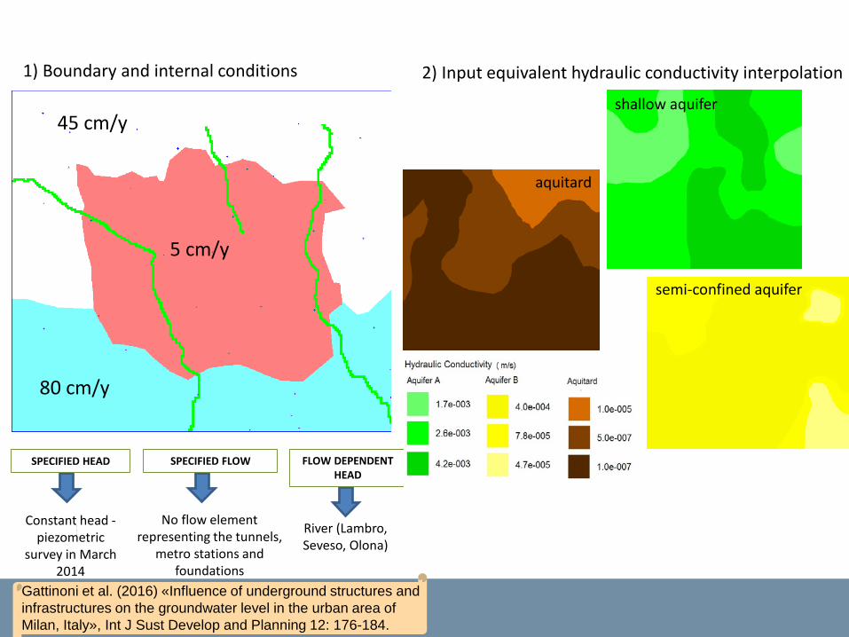
1) Boundary and internal conditions
Wells
No flow elements
Q well: ≈ 11 m3/s
SPECIFIED HEAD SPECIFIED FLOW FLOW DEPENDENT HEAD
Constant head -piezometric
survey in March 2014
River (Lambro, Seveso, Olona)
No flow elementrepresenting the tunnels,
metro stations and foundations
2) Input equivalent hydraulic conductivity interpolation
45 cm/y
5 cm/y
80 cm/y
shallow aquifer
semi-confined aquifer
aquitard
Gattinoni et al. (2016) «Influence of underground structures and infrastructures on the groundwater level in the urban area of Milan, Italy», Int J Sust Develop and Planning 12: 176-184.
Average hydraulic gradient ≈ 1% Local hydraulic gradient ≈ 20% Hydraulic gradient for suffusion ≈ 40%
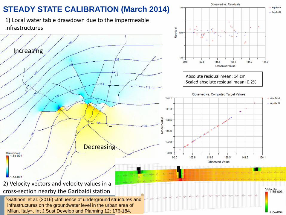
STEADY STATE CALIBRATION (March 2014)
Absolute residual mean: 14 cmScaled absolute residual mean: 0.2%
1) Local water table drawdown due to the impermeableinfrastructures
2) Velocity vectors and velocity values in a cross-section nearby the Garibaldi station
Increasing
Decreasing
Gattinoni et al. (2016) «Influence of underground structures and infrastructures on the groundwater level in the urban area of Milan, Italy», Int J Sust Develop and Planning 12: 176-184.

Probability distributions of: (a) the recharge multiplying factor(b) the withdrawal decreasing
Stochastic modelling of groundwater flow for hazard assessment along the underground infrastructures in Milan (northern Italy)
Gattinoni et al. (2018) «Stochastic modelling of groundwater flow for hazard assessment along the underground infrastructures in Milan (northern Italy)», TUST (in press).

Average groundwater rise simulated with the stochastic approach
Metro station Scenario∆H50% ∆H75% ∆H95%
Garibaldi1 3.12 3.38 4.13Repubbl.2 2.93 3.14 3.34P.Venezia1 2.71 2.89 3.09Domodos.2 3.08 3.28 3.53Centrale1 2.99 3.2 3.42
Lotto1 3.20 3.41 3.69Cadorna1 2.81 3.01 3.19Duomo3 2.60 2.79 2.95Loreto2 2.76 2.95 3.18Piola2 2.56 2.95 2.97Zara2 3.03 2.74 3.49
Lambrate2 2.51 3.25 2.92
Water table changes (in m) in some metro stations: ∆H50%, ∆H75% and ∆H95%are respectively the 50%, 75% and 95% percentiles of the simulated values.
Gattinoni et al. (2018) «Stochastic modelling of groundwater flow for hazard assessment along the underground infrastructures in Milan (northern Italy)», TUST (in press).

Probability occurrences of water table in some metro stations, compared to their bottom and top altitudes.
Gattinoni et al. (2018) «Stochastic modelling of groundwater flow for hazard assessment along the underground infrastructures in Milan (northern Italy)», TUST (in press).
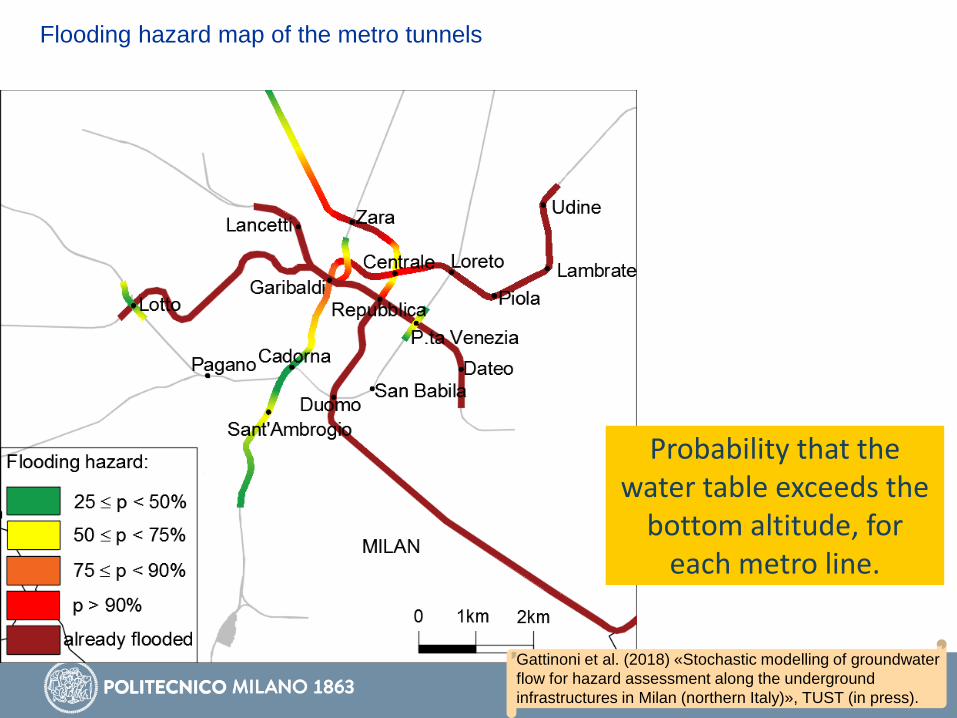
Flooding hazard map of the metro tunnels
Probability that the water table exceeds the
bottom altitude, for each metro line.
Gattinoni et al. (2018) «Stochastic modelling of groundwater flow for hazard assessment along the underground infrastructures in Milan (northern Italy)», TUST (in press).

MITIGATION SOLUTIONS
RECHARGE MODIFICATION:- Decreasing of infiltration rate
in the domain (parasite water reduction, bettermanagement of irrigationchannels, etc.)
- Restoration of the originalhydraulic connection of the surface network
PUMPING MODIFICATION:- Increasing pumping rate in
aquifer A (10%-30%)
DRAINAGE TUNNEL:- floodway-diverter of the
Seveso River
Gattinoni & Scesi (2017) «The groundwater rise in the urban area of Milan and its interactiosn with underground structures and infrastructures», TUST 62: 103-114.

MITIGATION SOLUTIONS
Scenario Hypotesis ∆h (m)
Area of interest
I1 Recharge reduction 25%in the whole domain
-0.7 Highest values equal to -1m in the western zoneof Milan
I2 Draining tunnel (totaldischarge ≈ 2 m3/s)
-2.5 Highest values equal to -5 m nearby the tunnel
I3_10 Pumping rate increase of10% in aquifer A
-0.3 Located in the centralarea of Milan
I3_30 Pumping rate increase of30% in aquifer A
-1.0 Located in the centralarea of Milan
I1+I2 Superimposition ofscenarios I1 and I2
-3.0 Similar to scenario I2 butwith a larger extensionof the drawdown
I1+I3_30 Superimposition ofscenarios I1 and I3_30
-1.5 Generalized over thewhole domain, with maxvalues in the central area
Non-structural measures can easily manage the short term hazard, whereas in the long term an integration between structural and non-structural measures will be necessary.
Gattinoni & Scesi (2017) «The groundwater rise in the urban area of Milan and its interactiosn with underground structures and infrastructures», TUST 62: 103-114.

A drainage system located at the bottom of the metro tunnels would havekept the water table below the infrastructures, avoiding this kind of hazard.
Prevention would have been the best solution!
Gattinoni & Scesi (2017) «The groundwater rise in the urban area of Milan and its interactiosn with underground structures and infrastructures», TUST 62: 103-114.

Hydrogeological model is a key factor in geological hazard assessment and prevention!
Learn from yesterday, Live for today,Hope for tomorrow.The important thing is not to stop questioning
Albert Einstein
Maierato landslide
Thank you for your attention!Sempione tunnel


