34
Hydrological network detection for SWOT data S. Lobry, F. Cao, R. Fjortoft, JM Nicolas, F. Tupin IRS SPU – avril 2016
Hydrological network detection for
SWOT data
S. Lobry, F. Cao, R. Fjortoft, JM Nicolas, F. Tupin
IRS SPU – avril 2016

SWOT mission
Large water bodies detection
Fine network detection
Further works
page 1

SWOT mission
SWOT
• Surface Water and Ocean Topography
• Hydrology: estimation of the river and lake volumes,
reservoirs, wetlands for a better understanding of the
global water cycle
• Oceanography: global measurements of ocean surface
topography with high spatial resolution to improve ocean
circulation models (weather prediction, climate,
navigation,…)
• NASA / CNES mission
• Launch planned in 2020
page 2

SWOT mission
Specifications (images)
• Altimetry with interferometric
SAR
• KaRIn instrument (Ka band
radar interferometer): single
pass interferometry
• Angles : 1° to 4°
• Ka band : 8.6mm
• Temporal cycle : every point
on the earth measured twice
every 21 days
page 3 http://swot.jpl.nasa.gov/

page 4 ©SWOT présentation, JC Souyris, CNES

page 5 ©SWOT présentation, JC Souyris, CNES

SWOT – specifications
Use of Ka band (8.6mm)
• Interferometric sensitivity depends
on basis / λ
• High sensitivity to object roughness
• Sensitivity to tropospheric
conditions
Very small incidence angle
([0.6°,4°])
• Lay-over effects
• Range resolution variation
• Strong land / water contrast
page 6 ©SWOT présentation, JC Souyris, CNES

Mission SWOT
page 7 http://swot.jpl.nasa.gov/

KaRIn / SWOT requirements for water
detection
Water bodies
• Whose surface area /width exceeds 250x250 m² /
100m
• In region of moderate topographic relief
Issues
• Variable water / land contrast, speckle impact
• Position and orientation of the river in the swath
• Pollution by other features ? (roads ?)
page 8

SWOT mission – ADT
Challenges for the Algorithm Definition Team
• Fast and reliable processing methods for
- River and water bodies detection
- Height estimation (interferometric phase)
• Difficulties :
- Fine networks
- Speckle
- Geometric deformations
- Simulated data
page 9
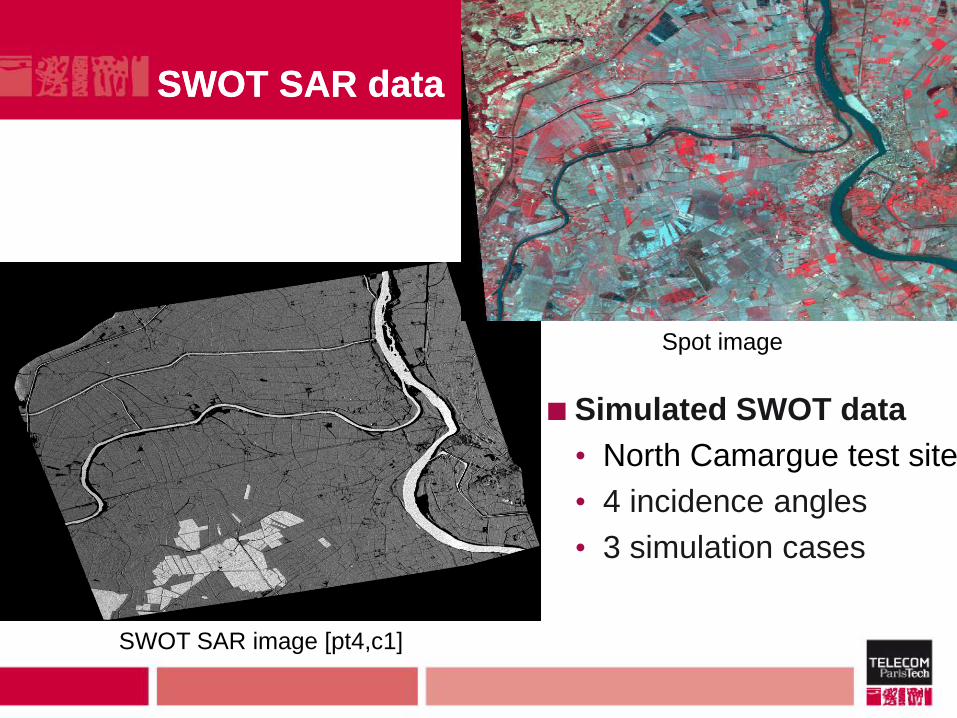
SWOT SAR data
Spot image
SWOT SAR image [pt4,c1]
SWOT SAR data
Simulated SWOT data
• North Camargue test site
• 4 incidence angles
• 3 simulation cases

Incidence angle 1 ° 2 ° 3° 4° [pt1] [pt2] [pt3] [pt4]

Incidence angle 1 ° 2 ° 3° 4° [pt1] [pt2] [pt3] [pt4]

SWOT mission
Large water bodies detection
Fine network detection
Further works
page 13

SAR data and statistics
Data: complex electro-magnetic field
(amplitude , , intensity )
Speckle: coherent imagery, interferences
• Goodman model (rough surfaces)
page 14

SAR data and statistics
One channel, Goodman model:
• Multi-look images:
• Intensity distribution: Gamma
• Amplitude distributions: Rayleigh-Nakagami
page 15

SAR data and statistics
D channels, Goodman model:
• Vectorial data:
• Circular complex Gaussian distribution:
page 16

SAR data and statistics
Multi-look data, Goodman model: Wishart distribution
page 17
coherence phase

SAR data and statistics
page 18
D=1
Amplitude data
(classification, object
recognition,…)
D=2
different incidence angles
Interferometric data:
geometric information
(elevation, movement)
D=3
different polarizations
Polarimetric data
Backscattering mechanisms
(classification, object recognition,…)
@DLR
@DLR
@ONERA
@RadarSat2

InSAR data
page 19

Probabilistic framework
Bayesian classification
• Two classes : water / background
• Distributions of the SAR signals taken into account
• Regularization term
page 20

Probabilistic framework
Refinement
• Local learning of the class
parameters
• Image partitioning for graph-cut
based optimization
page 21

page 22
Thèse S. Lobry
SWOT mission
Large water bodies detection
Fine network detection
Further works
page 23

Fine network detection
Context:
• Adaptation of a road detection algorithm for SAR data
Method principle:
• Low-level line detector taking into account SAR
statistics
• High level step connecting the detected candidates
(contextual information)
page 24

page 25
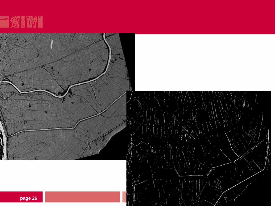
Step 1: Line detector
Speckle noise:
• Nakagami distribution of SAR amplitude data
• Line detector based on the ratio of amplitude mean
computed on stripes around the considered
structure
• Statistical analysis of the ditribution of the ratio-
based line detector
• In practice:
- Width of the line between 3 and 5 pixels
- 11 pixels length
page 26

page 27
Step 2:Markov random field on a line graph
Graph construction:
• Line detection
• Graph = segment graph using the detected segments and all
the « possible » connexions (edge = 2 segments share an
extremity)
Nodes of G
Edges of G
Detected seg.
Added seg.
extremity
Image representation Graph representation

page 28
0 ou 1
?

page 29
Markovian energy
• X binary field (road or not road label)
• Y line detector responses observed in the SAR data
s c
ccss xVxyPyxU )()|(log)|(
Likelihood of the observations for
a given label
Computed using the line detector
response along the segment
Prior information
about the river shapes
•Riverss are long
•Curvature
•Few crossings
Step 2:Markov random field on a line graph

Quantitative evaluation (correctness / completeness):
• Water bodies / networks
• Positioning problems between mask / detection
Some results
SWOT mission
Large water bodies detection
Fine network detection
Conclusion and further works
page 31
Conclusion and further works
Joint analysis of phase / amplitude data
• Combining both information (using complex field
distributions – phase / coherence / amplitude)
Introduction of « prior » information
• Reference mask deformation (level set)
• Multi-temporal processing (class learning, algorithm
initialization, multi-temporal denoising, …)
Constraint: huge amount of data
• Simple and fast algorithms to compute the products
page 32

References
• S. Lobry et al., Non uniform MRF for classification of SAR images,
EUSAR 2016
• R. Fjortoft et al. KaRIn on SWOT: Characteristics of Near-Nadir Ka-
Band Interferometric SAR Imagery, IEEE TGRS, 2014.
• F. Cao et al., Extraction of water surface in simulated Ka-band SAR
images of KaRIN on SWOT , IGARSS 2011.
• M. Negri et al., Junction-Aware Extraction and Regularization of Road
Networks in SAR Images, IEEE TGRS 2006
• R. Fjortoft et al. Unsupervised classification of radar images using
hidden Markov chains and hidden Markov random fields. IEEE TGRS
2003.
• F. Tupin et al. , Linear Feature Detection on SAR Images: Application
to the Road Network, IEEE TGRS 1998
page 33


