Chapter 3 INFILTRATION I. INTRODUCTION Infiltration is commonly defined as the process of water entry at the land surface into a soil from a source such as rainfall, irrigation, or snowmelt. The rate of infiltration is generally controlled by the rate of soil water movement below the surface. Rainfall excess is the portion of applied water that leaves the surface site not as infiltration but as runoff. As can be seen in Figure 3.1, the classic components of the hydrologic cycle for an event are 1) evaporation, 2) interception and depression storage, 3) infiltration, and 4) rainfall excess. The difference between rainfall excess and infiltration models is that rainfall excess models lump the losses (infiltration, evaporation, interception, and depression storage) together while infiltration models only describe the infiltration portion. Since evaporation, interception, and depression storage are normally minor compared to the infiltration portion during an event, rainfall excess models can be considered synonymous with infiltration models. This chapter of the handbook presents current knowledge and practice of modeling infiltration and rainfall excess. II. PRINCIPLES OF INFILTRATION The time-dependent rate of infiltration into a soil is governed by the Richards Equation (Richards, 1931), subject to given antecedent soil moisture conditions in the soil profile, the rate of water application at the soil surface, and the conditions at the bottom of the soil profile. In general, the initial soil water potential varies with soil depth, z. The initial conditions) at time t equal 0 and can be expressed as follows h(z,t) = f(z); t = 0 (3.1) where the profile of matric potential head (h) varies with depth (z). The boundary condition at the soil surface depends upon the rate of water application. For a rainfall event with intensities less than or equal to the saturated hydraulic conductivity of the soil profile, all the rain infiltrates into the soil without generating any runoff. For higher rainfall intensities, all the rain infiltrates into the soil during early stages until the soil surface becomes saturated. After this point, the infiltration is less than the rain intensity and runoff begins. These conditions may be expressed as: (3.2) h = h 0 ; (3.3) where R is the rainfall intensity, ho is a small positive ponding depth on the soil surface, and t p is the ponding time. These conditions also accommodate time varying rainfall intensities, as well as when 75 Hydrology Handbook Downloaded from ascelibrary.org by The University of Queensland Library on 06/04/14. Copyright ASCE. For personal use only; all rights reserved.
Transcript
Chapter 3
INFILTRATION
I. INTRODUCTION
Infiltration is commonly defined as the process of water entry at the land surface into a soil from asource such as rainfall, irrigation, or snowmelt. The rate of infiltration is generally controlled by the rateof soil water movement below the surface. Rainfall excess is the portion of applied water that leaves thesurface site not as infiltration but as runoff. As can be seen in Figure 3.1, the classic components of thehydrologic cycle for an event are 1) evaporation, 2) interception and depression storage, 3) infiltration,and 4) rainfall excess. The difference between rainfall excess and infiltration models is that rainfall excessmodels lump the losses (infiltration, evaporation, interception, and depression storage) together whileinfiltration models only describe the infiltration portion. Since evaporation, interception, and depressionstorage are normally minor compared to the infiltration portion during an event, rainfall excess modelscan be considered synonymous with infiltration models. This chapter of the handbook presents currentknowledge and practice of modeling infiltration and rainfall excess.
II. PRINCIPLES OF INFILTRATION
The time-dependent rate of infiltration into a soil is governed by the Richards Equation (Richards,1931), subject to given antecedent soil moisture conditions in the soil profile, the rate of water applicationat the soil surface, and the conditions at the bottom of the soil profile. In general, the initial soil waterpotential varies with soil depth, z. The initial conditions) at time t equal 0 and can be expressed as follows
h(z,t) = f(z); t = 0 (3.1)
where the profile of matric potential head (h) varies with depth (z).The boundary condition at the soil surface depends upon the rate of water application. For a rainfall
event with intensities less than or equal to the saturated hydraulic conductivity of the soil profile, all therain infiltrates into the soil without generating any runoff. For higher rainfall intensities, all the raininfiltrates into the soil during early stages until the soil surface becomes saturated. After this point, theinfiltration is less than the rain intensity and runoff begins. These conditions may be expressed as:
(3.2)
h = h0; (3.3)
where R is the rainfall intensity, ho is a small positive ponding depth on the soil surface, and tp is theponding time. These conditions also accommodate time varying rainfall intensities, as well as when
75
Hydrology Handbook
Dow
nloa
ded
from
asc
elib
rary
.org
by
The
Uni
vers
ity o
f Q
ueen
slan
d L
ibra
ry o
n 06
/04/
14. C
opyr
ight
ASC
E. F
or p
erso
nal u
se o
nly;
all
righ
ts r
eser
ved.
76 HYDROLOGY HANDBOOK
Figure 3.1.—Schematic of Rainfall Excess Components (Sabol et al, 1992).
rainfall intensity is smaller than the saturated hydraulic conductivity (Ks) of the soil throughout thestorm. For a surface ponded-water irrigation, condition Equation 3.3 will apply from time zero on.
The surface boundary conditions equations 3.2 and 3.3 apply at any point in the field during rainfall.In a long sloping field, some infiltration may continue to occur in lower parts of the field even after therainfall stops, due to continued overland flow from upper parts. During this phase, conditions describedby equations 3.2 and 3.3 still apply after rainfall is replaced by the overland flow per unit area at the pointof interest. To obtain the overland flow rates, hydrodynamic equations of overland flow need to be solvedinteractively with infiltration (Woolhiser, et al., 1990).
The lower boundary condition depends upon the depth of the unsaturated profile. For a deep profile,a unit-gradient flux condition is commonly applied at a depth, L, below the infiltration-wetted zone:
q(L,t) = K(8,L); t > 0.
For a shallow profile, a constant pressure head is assumed at the water table depth L:
h(L, t) = 0; t > 0.
(3.4)
(3.5)
The Richards Equation 3.1 subject to the general conditions described in Equations 3.2 to 3.5 in alayered soil profile does not have any known analytical or closed-form solutions for infiltration. How-ever, the solutions can be obtained by using finite-difference or finite-element numerical methods (Rubinand Steinhart, 1963; Mein and Larson, 1973).
For non-layered soils, uniform initial soil moisture distribution, and limited surface boundary condi-tions, some closed-form solutions are available. The pioneering work of Philip (1957) provided a seriessolution for vertical infiltration into a semi-infinite homogeneous soil, with a constant initial moisturecontent @j and a constant matric potential ho maintained at the soil surface. Recently, Swartzendruber(1987) presented a solution that holds for both small to intermediate and large times.
III. FACTORS AFFECTING INFILTRATION/RAINFALL EXCESS
Factors which affect infiltration have been divided into the following categories: 1) Soil; 2) Surface; 3)Management; and 4) Natural (Brakensiek and Rawls, 1988). Depending on their importance for thespecific application, these categories should be accounted for when applying infiltration models. Pub-lished research results are used to illustrate the relative importance of the various factors. Methods forincorporating the effects of the factors into infiltration models will be discussed in the Infiltration/Rain-fall Excess Models for Practical Applications section.
Hydrology Handbook
Dow
nloa
ded
from
asc
elib
rary
.org
by
The
Uni
vers
ity o
f Q
ueen
slan
d L
ibra
ry o
n 06
/04/
14. C
opyr
ight
ASC
E. F
or p
erso
nal u
se o
nly;
all
righ
ts r
eser
ved.
INFILTRATION 77
A. Soil
Soil factors encompass both soil physical properties including particle size, morphological, and chemi-cal properties and soil water properties including soil water content, water retention characteristic, andhydraulic conductivity. Soil water properties are closely related to soil physical properties.
1. Soil Physical Propertiesa. Soil Texture. Soil texture is determined from the size distribution of individual particles in a soil
sample. Soil particles smaller than 2 mm are divided into three soil texture groups: sand, silt, and clay.Fig. 3.2 shows the particle size, sieve dimension, the defined size class, and the limits for the basic soiltexture classes for the U.S. Department of Agriculture (USDA) (Soil Conservation Service, 1982b). The soiltexture groups which have the greatest effect on infiltration (Rawls et al., 1991) are the percentages of sand,silt, clay, fine sand, coarse sand, very coarse sand, and coarse fragments (0.2 cm). Fig. 3.3a and 3.3b illustratethat coarse textured soils (gravelly sandy loam) normally have a higher infiltration rate than fine texturedsoils (clay loam). Coarse fragments in the soil normally increase the infiltration rate of the soil.
b. Morphological Properties. The morphological properties having the greatest effect on infiltration arebulk density, organic matter, and clay type. These properties are closely related to soil structure and soilsurface area. As bulk density increases, soil porosity and infiltration decrease. Soil organic matter (1.74
Figure 3.3a.—Infiltration Curves for the Artemisa arbuscula/Poa secunda (low)Community, Coils Creek Watershed, Clay Loam (Blackburn,1973).
Figure 3.3b.—Infiltration Curves for Symphoricarpos longiflorus/Artemisiatridentata/Agropyron spicatum/Wyethia mollius Community,Coils Creek Watershed, Gravelly Sandy Loam (Blackburn, 1973).
times the percent of organic carbon) is inversely related to bulk density; thus as organic matter increases,infiltration increases.
The clay mineralogy, or clay type, has a significant effect on infiltration for soils containing a largepercentage of clay (10%). For example, expandable clays such as montmorillionitic have a significantlylower infiltration rate than nonexpendable clays such as kaolinitic.
Soil layers due to natural profile development, crusts, or compaction limit or modify infiltration rates.Fig. 3.4 illustrates that a soil with a porous layer overlying a less porous layer results in a final infiltrationrate that approaches the final rate of the lower layer. Also, the crusted surface, which is synonymous toa less porous layer overlying a more porous layer, produces a significantly lower final infiltration rate.
Macroporosity is natural or man-induced through "channels" connected from the soil surface to somedepth in the soil profile. They may be cracks, worm holes, tillage marks, or intentional soil slots. Fig. 3.5shows that compaction severely reduces the volume of macroscopic porosity and reduces infiltration rates.Natural cracks in a montmorillonitic clay can increase the infiltration rate from 0.05 cm/hr to over 5 cm/hr.
Other morphological properties such as the thickness of the soil horizon and soil structure are derivedfrom soil survey descriptions and a quantitative description of their effects on soil water movement havenot been determined.
c. Chemical Properties. Chemical properties of the soil are important because they affect the integrityof the soil aggregates (group of soil particles bound together). Chemical soil properties should be
Hydrology Handbook
Dow
nloa
ded
from
asc
elib
rary
.org
by
The
Uni
vers
ity o
f Q
ueen
slan
d L
ibra
ry o
n 06
/04/
14. C
opyr
ight
ASC
E. F
or p
erso
nal u
se o
nly;
all
righ
ts r
eser
ved.
Figure 3.4.—Infiltration Rate for: a) Uniform Soil, b) With a More PorousUpper Layer, and c) Soil Covered With a Surface Crust(HUM, 1971).
Figure 3.5.—a) Infiltration Rates, b) Volume of Macroscopic Pores, and c) SoilBulk Density Influenced by Soil; Compaction (Lull, 1959).
79
Hydrology Handbook
Dow
nloa
ded
from
asc
elib
rary
.org
by
The
Uni
vers
ity o
f Q
ueen
slan
d L
ibra
ry o
n 06
/04/
14. C
opyr
ight
ASC
E. F
or p
erso
nal u
se o
nly;
all
righ
ts r
eser
ved.
80 HYDROLOGY HANDBOOK
considered when they are outside normal ranges (Rawls, et al., 1991). Also, chemistry of the infiltratingwater can have an effect on infiltration.
2. Soil Water Propertiesa. Soil Water Content. Fig. 3.3a and 3.3b illustrate that the higher the water content the smaller the
infiltration rate.
b. Water Retention Characteristic. The water retention characteristic of the soil describes the soil'sability to store and release water and is defined as the relationship between the soil water content andthe soil suction or matric potential. Fig. 3.6 illustrates the water retention relationship for two contrastingsoil textures. Note that the sandy loam soil retains less water than the clay soil.
c. Hydraulic Conductivity. The hydraulic conductivity is the ability of the soil to transmit water anddepends upon both the properties of the soil and the fluid (Klute and Dirkson, 1986). Total porosity, poresize distribution, and pore continuity are the important soil characteristics affecting hydraulic conductiv-ity. The hydraulic conductivity at or above the saturation point is referred to as "saturated hydraulicconductivity" and is directly related to infiltration.
The hydraulic conductivity of the sandy loam soil decreases more rapidly with decrease in matrixpotential than the hydraulic conductivity of clay soil. Thus, at lower matrix potential (or higher suctions)the hydraulic conductivity of the clay soil is higher. The rate of change of matrix potential in the sandysoil also decreases much more rapidly than that of the clay soil.
Hysteresis is caused by entrapment of air in the soil during wetting, and can cause the hydraulicconductivity to decrease; however, its effect is normally small and for practical applications has mostlybeen neglected.
Figure 3.6.—The h(Q) Relationship of Sandy loam and Clayey Horizonsof Cecil Soil (Ahuja et al, 1985).
Hydrology Handbook
Dow
nloa
ded
from
asc
elib
rary
.org
by
The
Uni
vers
ity o
f Q
ueen
slan
d L
ibra
ry o
n 06
/04/
14. C
opyr
ight
ASC
E. F
or p
erso
nal u
se o
nly;
all
righ
ts r
eser
ved.
INFILTRATION 81
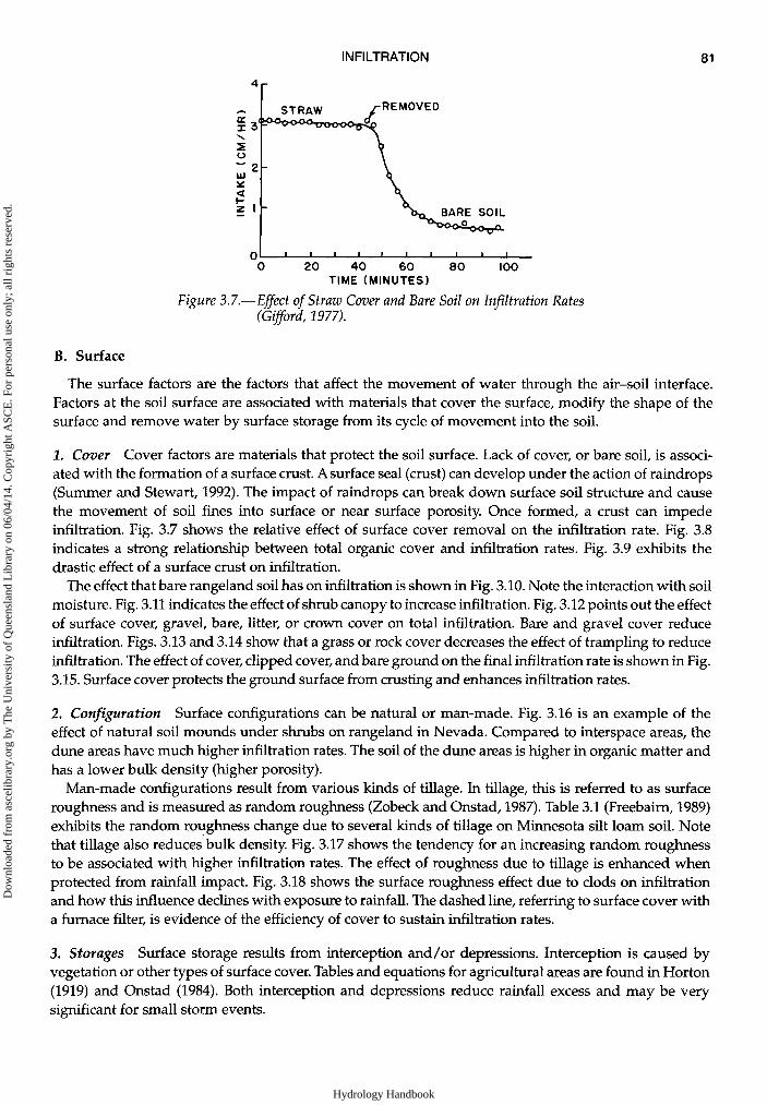
Figure 3.7.—Effect of Straw Cover and Bare Soil on Infiltration Rates(Gifford, 1977).
B. Surface
The surface factors are the factors that affect the movement of water through the air-soil interface.Factors at the soil surface are associated with materials that cover the surface, modify the shape of thesurface and remove water by surface storage from its cycle of movement into the soil.
1. Cover Cover factors are materials that protect the soil surface. Lack of cover, or bare soil, is associ-ated with the formation of a surface crust. A surface seal (crust) can develop under the action of raindrops(Summer and Stewart, 1992). The impact of raindrops can break down surface soil structure and causethe movement of soil fines into surface or near surface porosity. Once formed, a crust can impedeinfiltration. Fig. 3.7 shows the relative effect of surface cover removal on the infiltration rate. Fig. 3.8indicates a strong relationship between total organic cover and infiltration rates. Fig. 3.9 exhibits thedrastic effect of a surface crust on infiltration.
The effect that bare rangeland soil has on infiltration is shown in Fig. 3.10. Note the interaction with soilmoisture. Fig. 3.11 indicates the effect of shrub canopy to increase infiltration. Fig. 3.12 points out the effectof surface cover, gravel, bare, litter, or crown cover on total infiltration. Bare and gravel cover reduceinfiltration. Figs. 3.13 and 3.14 show that a grass or rock cover decreases the effect of trampling to reduceinfiltration. The effect of cover, clipped cover, and bare ground on the final infiltration rate is shown in Fig.3.15. Surface cover protects the ground surface from crusting and enhances infiltration rates.
2. Configuration Surface configurations can be natural or man-made. Fig. 3.16 is an example of theeffect of natural soil mounds under shrubs on rangeland in Nevada. Compared to interspace areas, thedune areas have much higher infiltration rates. The soil of the dune areas is higher in organic matter andhas a lower bulk density (higher porosity).
Man-made configurations result from various kinds of tillage. In tillage, this is referred to as surfaceroughness and is measured as random roughness (Zobeck and Onstad, 1987). Table 3.1 (Freebairn, 1989)exhibits the random roughness change due to several kinds of tillage on Minnesota silt loam soil. Notethat tillage also reduces bulk density. Fig. 3.17 shows the tendency for an increasing random roughnessto be associated with higher infiltration rates. The effect of roughness due to tillage is enhanced whenprotected from rainfall impact. Fig. 3.18 shows the surface roughness effect due to clods on infiltrationand how this influence declines with exposure to rainfall. The dashed line, referring to surface cover witha furnace filter, is evidence of the efficiency of cover to sustain infiltration rates.
3. Storages Surface storage results from interception and/or depressions. Interception is caused byvegetation or other types of surface cover. Tables and equations for agricultural areas are found in Horton(1919) and Onstad (1984). Both interception and depressions reduce rainfall excess and may be verysignificant for small storm events.
Hydrology Handbook
Dow
nloa
ded
from
asc
elib
rary
.org
by
The
Uni
vers
ity o
f Q
ueen
slan
d L
ibra
ry o
n 06
/04/
14. C
opyr
ight
ASC
E. F
or p
erso
nal u
se o
nly;
all
righ
ts r
eser
ved.
82 HYDROLOGY HANDBOOK
Figure 3.8.—Relationship of Median Infiltration Rate Classes with TotalOrganic Cover (%), Edwards Plateau, TX (Thurow, 1985).
Figure 3.9.—Effect of Surface Sealing and Crusting on Infiltration Rate fora Zanesville Silt Loam (Skaggs and Khaleel, 1982).
C. Management
Management, as a factor affecting infiltration, modifies the soil properties or the soil surface condition.The effects of these factors have already been discussed in previous sections. In this section, the effect ofmanagement practices on infiltration will be presented.
Hydrology Handbook
Dow
nloa
ded
from
asc
elib
rary
.org
by
The
Uni
vers
ity o
f Q
ueen
slan
d L
ibra
ry o
n 06
/04/
14. C
opyr
ight
ASC
E. F
or p
erso
nal u
se o
nly;
all
righ
ts r
eser
ved.
INFILTRATION 83
Figure 3.10.—Impact of Percent Bare Soil on Infiltration Rates After VariousTime Intervals (Gifford, 1977).
Figure 3.11.—Impact on Shrub Canopy on Infiltration Rates AfterVarious Time Intervals (Gifford, 1977).
1. Agriculture Agricultural management systems involve different types of tillage, vegetation, andsurface cover. Fig. 3.19 illustrates tillage practices (moldboard plow, chisel plow, and no till) influence oninfiltration. Brakensiek and Rawls (1988) reported that moldboard plowing would increase soil porosityfrom 10 to 20% depending on soil texture and hence, increase infiltration rates over non-tilled soils. Rawls(1983) reported that increasing the organic matter of the soil lowers the bulk density, increases porosityand hence, increases the infiltration. Fig. 3.20 gives the steady-state infiltration rate of bare ground,soybean vegetation, and residue cover interactions for planting, midseason, and harvest. The bare soilsteady-state rate decreases between planting and midseason and remains stable primarily as a result ofcrusting. Residue maintains a high steady-state rate until harvest, while the canopy and canopy residuecombination increase the steady-state rate.
Table 3.2 (North Central Regional Committee 40,1979) presents a grouping of major Midwest agricul-tural soils under tillage or grass management. There is a tendency for the same soil under grass
Hydrology Handbook
Dow
nloa
ded
from
asc
elib
rary
.org
by
The
Uni
vers
ity o
f Q
ueen
slan
d L
ibra
ry o
n 06
/04/
14. C
opyr
ight
ASC
E. F
or p
erso
nal u
se o
nly;
all
righ
ts r
eser
ved.
84 HYDROLOGY HANDBOOK
Figure 3.12.—Relationship of Various Covers to Infiltration Rates(Gifford, 1977).
Figure 3.13.—Infiltration Rate at 30 Minutes as a Function of Rock Cover andTrampling (Dadkah and Gifford, 1980).
management to have higher infiltration rates than when under tilled management. Fig. 3.19 clearlydepicts the influence of tillage management on infiltration rates. Fig. 3.21 indicates that the influence oftillage management decreases as the surface is exposed to rainfall. A surface cover reduces the degrada-tion of the tillage affect. Rawls et al. (1983) developed a diagram from tillage data for estimating the effectof plowing to increase soil porosity, hence, increasing infiltration rates.
Additions to the soil that increase organic matter would increase infiltration. As shown in Fig. 3.11, thesoil area under shrubs where litter accumulates and soil organic matter increased supported higher
Hydrology Handbook
Dow
nloa
ded
from
asc
elib
rary
.org
by
The
Uni
vers
ity o
f Q
ueen
slan
d L
ibra
ry o
n 06
/04/
14. C
opyr
ight
ASC
E. F
or p
erso
nal u
se o
nly;
all
righ
ts r
eser
ved.
INFILTRATION 85
Figure 3.16.—Infiltration Curves for the Artemisia tridentata Community,Dickwater Watershed, Coppice Dune and Interspace(Blackburn, 1973).
Figure 3.14.—Infiltration Rate at 30 Minutes as a Function of Grass Coverand Trampling (Dadkhah and Gifford, 1980).
Figure 3.15.—Final Infiltration Rates Shown as a Mean From Five Sites inArizona and Nevada for Very Wet Runs with Natural, Clipped,and Bare Cover (Lane et al, 1987).
Hydrology Handbook
Dow
nloa
ded
from
asc
elib
rary
.org
by
The
Uni
vers
ity o
f Q
ueen
slan
d L
ibra
ry o
n 06
/04/
14. C
opyr
ight
ASC
E. F
or p
erso
nal u
se o
nly;
all
righ
ts r
eser
ved.
86 HYDROLOGY HANDBOOK
TABLE 3.1. Influence of Tillage on Random Roughness(Freebairn, 1989).
Port Byron silt loam-Lawler farm. Rochester, MN
Tillage methChiselplow
Moldboardplow
Fall chisel
Fall plow
PlotEFGHIJKL
AABBEEFF
RR beforetillagemm
999999997777
RR aftertillagemm
171816212219172524184227
Bulk denbefore
gm/cm3
1.161.161.161.161.161.161.161.161.161.161.161.16
Bulk denafter
gm/cm3
1.071.071.071.070.970.970.970.971.151.150.990.99
Figure 3.17.—Infiltration Rate vs. Roughness Index for Covered andExposed Agricultural Plots (Freebairn, 1989).
infiltration rates. Rawls (1983) reports organic matter to be a major factor that lowers the bulk density(increased porosity); hence, increasing organic matter increases the hydraulic conductivity.
2. Irrigation Many of the factors in previous sections apply to infiltration under irrigation practices.Sprinkler systems are similar to rainfall infiltration processes. Border irrigation is similar to pondedinfiltration processes. Furrow irrigation factors have been investigated by Trout and Kemper (1983) andby Kemper et al. (1988). Sub-irrigation systems involve factors common to soil moisture movement.
3. Rangeland The type of vegetation on rangelands is an important factor determining infiltrationrates. Fig. 3.22 reveals a major difference of mean infiltration rates for three vegetation types. In Fig. 3.23,a significant effect on total infiltration is seen between successional stages of rangeland vegetation. Fig.
Hydrology Handbook
Dow
nloa
ded
from
asc
elib
rary
.org
by
The
Uni
vers
ity o
f Q
ueen
slan
d L
ibra
ry o
n 06
/04/
14. C
opyr
ight
ASC
E. F
or p
erso
nal u
se o
nly;
all
righ
ts r
eser
ved.
INFILTRATION 87
Figure 3.18.—Infiltration Rates Webster Clay Loam with the SurfaceCovered with Various Percentages of 25-50 mm Clodsor Furnace Filter (Freebairn, 1989).
Figure 3.19.—Infiltration Rates for Port Byron Silt Loam, Two Months AfterChisel and Moldboard Plow Tillage and Four Months AfterPlanting Under No-till (Freebairn, 1989).
Hydrology Handbook
Dow
nloa
ded
from
asc
elib
rary
.org
by
The
Uni
vers
ity o
f Q
ueen
slan
d L
ibra
ry o
n 06
/04/
14. C
opyr
ight
ASC
E. F
or p
erso
nal u
se o
nly;
all
righ
ts r
eser
ved.
88 HYDROLOGY HANDBOOK
Figure 3.20.—Seasonal Effects of Agricultural Practices on Steady-StateInfiltration Rates (Rawls et al, 1993a).
3.24 shows an improvement of infiltration rates going from bare ground to grass to shrub vegetationtypes.
Grazing practices also influence infiltration. Fig. 3.25 provides evidence that grazing reduces the finalinfiltration rate. Heavy grazing is associated with a greater reduction of the final infiltration rate. Fromstudies in New Mexico, presented in Fig. 3.26, a difference is reported between several grazing treat-ments. Fig. 3.27 clarifies the effect of stocking density on infiltration rates. The effect of grazing systemson infiltration is shown in Fig. 3.28. The three grazing systems are MCG-moderate continuous, HCG-heavy continuous, and SDG-short duration grazing. Effects of rangeland improvements on runoff aresummarized in Rangeland Hydrology (Branson et al., 1981). Fig. 3.29 shows an effect of burning oninfiltration rates.
D. Natural
Natural factors include natural processes such as precipitation, freezing, change of seasons, tempera-ture, and moisture which vary with time and space and interact with other factors in their effect oninfiltration. The temporal and spatial variability effects will be discussed.
1. Temporal The effect of cumulative antecedent rainfall on exposed and 50% residue-covered agricul-tural soil is shown in Fig. 3.20, indicating a decrease in the steady-state infiltration rate with continuedexposure to the action of rainfall. For bare soil, it seems that a stable steady-state infiltration rate isachieved between planting and midseason, indicating that a stable crust is achieved early in the growingseason and maintained thereafter. Fig. 3.20 demonstrates that the steady-state infiltration rate increasesas canopy cover increases over the growing season. Also, Fig. 3.20 indicates that canopy cover andresidue cover do not cause additive increases in the steady-state infiltration rate.
Increases in rainfall intensity expand surface disturbance caused by the rain drops and the buildup ofa ponding head. This usually increases the bare soil infiltration. For bare soil with canopy cover, thisintensity effect is dissipated by the growing crop canopy.
Soil temperature influences infiltration through its effect on the viscosity of water. Lee (1983) foundthat freezing the soil with a high moisture content decreases infiltration to almost zero, while freezingthe soil at a low moisture content increases infiltration by twice its normal rate.
Hydrology Handbook
Dow
nloa
ded
from
asc
elib
rary
.org
by
The
Uni
vers
ity o
f Q
ueen
slan
d L
ibra
ry o
n 06
/04/
14. C
opyr
ight
ASC
E. F
or p
erso
nal u
se o
nly;
all
righ
ts r
eser
ved.
INFILTRATION 89
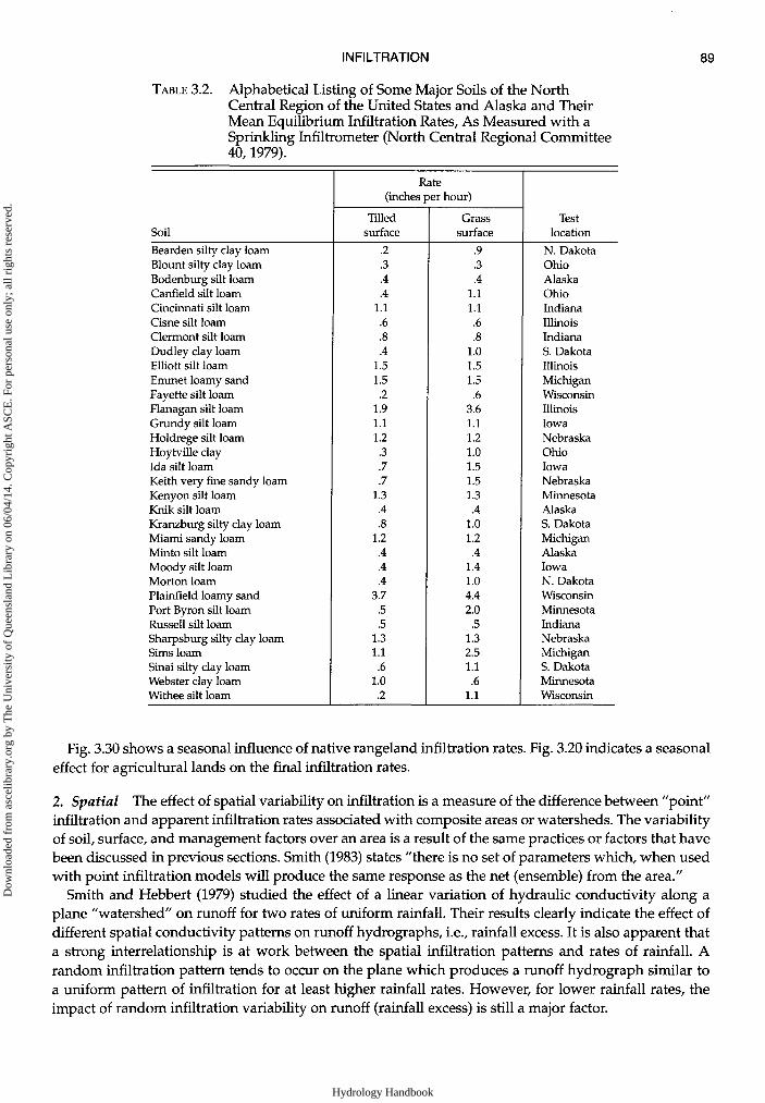
TABLE 3.2. Alphabetical Listing of Some Major Soils of the NorthCentral Region of the United States and Alaska and TheirMean Equilibrium Infiltration Rates, As Measured with aSprinkling Infiltrometer (North Central Regional Committee40,1979).
N. DakotaOhioAlaskaOhioIndianaIllinoisIndianaS. DakotaIllinoisMichiganWisconsinIllinoisIowaNebraskaOhioIowaNebraskaMinnesotaAlaskaS. DakotaMichiganAlaskaIowaN. DakotaWisconsinMinnesotaIndianaNebraskaMichiganS. DakotaMinnesotaWisconsin
Fig. 3.30 shows a seasonal influence of native rangeland infiltration rates. Fig. 3.20 indicates a seasonaleffect for agricultural lands on the final infiltration rates.
2. Spatial The effect of spatial variability on infiltration is a measure of the difference between "point"infiltration and apparent infiltration rates associated with composite areas or watersheds. The variabilityof soil, surface, and management factors over an area is a result of the same practices or factors that havebeen discussed in previous sections. Smith (1983) states "there is no set of parameters which, when usedwith point infiltration models will produce the same response as the net (ensemble) from the area."
Smith and Hebbert (1979) studied the effect of a linear variation of hydraulic conductivity along aplane "watershed" on runoff for two rates of uniform rainfall. Their results clearly indicate the effect ofdifferent spatial conductivity patterns on runoff hydrographs, i.e., rainfall excess. It is also apparent thata strong interrelationship is at work between the spatial infiltration patterns and rates of rainfall. Arandom infiltration pattern tends to occur on the plane which produces a runoff hydrograph similar toa uniform pattern of infiltration for at least higher rainfall rates. However, for lower rainfall rates, theimpact of random infiltration variability on runoff (rainfall excess) is still a major factor.
Hydrology Handbook
Dow
nloa
ded
from
asc
elib
rary
.org
by
The
Uni
vers
ity o
f Q
ueen
slan
d L
ibra
ry o
n 06
/04/
14. C
opyr
ight
ASC
E. F
or p
erso
nal u
se o
nly;
all
righ
ts r
eser
ved.
90 HYDROLOGY HANDBOOK
RAINFALL SINCE TILLAGE (mm)
Figure 3.21.—Infiltration Rates vs. Antecedent Rainfall Since Tillage forCovered and Exposed Plots, Webster Clay Loam (Freebairn,1989).
Figure 3.22.—Mean Infiltration Rates for Three Vegetation Types,Edwards Plateau, TX (Thurow et al, 1986).
Hydrology Handbook
Dow
nloa
ded
from
asc
elib
rary
.org
by
The
Uni
vers
ity o
f Q
ueen
slan
d L
ibra
ry o
n 06
/04/
14. C
opyr
ight
ASC
E. F
or p
erso
nal u
se o
nly;
all
righ
ts r
eser
ved.
INFILTRATION 91
Figure 3.23.—Infiltration Amounts for Four Successional Stages ofRangelandVegetation (Gifford, 1977).
III. INFILTRATION/RAINFALL EXCESS MODELS FOR PRACTICAL APPLICATIONS
Infiltration models for field applications usually employ simplified concepts which predict the infiltra-tion rate or cumulative infiltration volume. This assumes that surface ponding begins when the surfaceapplication rate exceeds the soil surface infiltration rate. The rainfall excess models that lump all losses(infiltration, depression storage, interception) are strictly empirical models.
A. Rainfall Excess Models
Rainfall excess is the part of rainfall that is not lost to infiltration, depression storage, and interception.While a number of models have been proposed for estimating rainfall excess, the most commonly-usedmodels are the index models and the SCS curve number model.
Index models are relatively simple methods that can be useful when performing gaged analysis (e.g.,when rainfall and runoff data are available) or when a simple method is commensurate with the dataavailable for estimating loss values. The most commonly used index models are 1) phi index, 2) initialand constant loss rate and 3) constant proportion loss rate (Pilgrim and Cordery, 1992).
1. Phi Index The phi index, c|>, is probably the most widely used index model. The loss rate defined bythe phi index is shown in Fig. 3.31 and is described mathematically as
f(t), = I(t), forl(t)«t>, (3-6)
where f(t) is the loss rate, I(t) is the rainfall intensity, t is time, and <|> is a constant called the $ index. Thephi index can be estimated from storm data by separating baseflow from the total runoff and thendetermining the <j> which causes the rainfall excess to equal the total runoff. The advantage of this method
Figure 3.25.—Relationships Between Final Infiltration Rates on Heavily GrazedAreas (Gifford and Hawkins, 1978).
Hydrology Handbook
Dow
nloa
ded
from
asc
elib
rary
.org
by
The
Uni
vers
ity o
f Q
ueen
slan
d L
ibra
ry o
n 06
/04/
14. C
opyr
ight
ASC
E. F
or p
erso
nal u
se o
nly;
all
righ
ts r
eser
ved.
93
Figure 3.26.—Mean Infiltration Rates for Various Grazing Treatmentsat Fort Stanton, NM (Weltz and Wood, 1986).
Figure 3.27.—Mean Infiltration Rates for Pastures Grazed at Three StockingDensities (Warren et al, 1986).
is that it requires only a single parameter. The disadvantages are that it requires rainfall runoff recordsand the <j> is dependent on the watershed and storm conditions from which it was determined.
2. Initial and Constant Loss Rate The loss rate function associated with this procedure is shown inFig. 3.32 and is described mathematically as
(3.7)
INFILTRATION
forfoi
for
Hydrology Handbook
Dow
nloa
ded
from
asc
elib
rary
.org
by
The
Uni
vers
ity o
f Q
ueen
slan
d L
ibra
ry o
n 06
/04/
14. C
opyr
ight
ASC
E. F
or p
erso
nal u
se o
nly;
all
righ
ts r
eser
ved.
94 HYDROLOGY HANDBOOK
Figure 3.28.—Infiltration Rates for Three Grazing Systems on the EdwardsPlateau: MCG-Moderate Continuous, HCG-Heavy Continuous,and SDG-Short Duration (Thurow, 1985).
where P(t) is the cumulative rainfall volume at time t from the beginning of rainfall, I(t) is the rainfallintensity, IA is the initial loss, and C is the constant loss rate. This method is a crude approximation to atypical infiltration curve that decays from some initial high rate to a final constant infiltration rate. Theinitial loss might be considered to represent the total loss due to surface factors and volume infiltratedprior to attaining the soils long-term infiltration rate. This method is similar to the phi index and hassimilar advantages and disadvantages. Table 3.3 presents some currently used loss rates (Sabol et al.,1992).
3. Constant Proportion Loss Rate The loss rate function associated with this procedure is shown inFig. 3.33 and is described mathematically as
f(t) = CP * I(t), (3.8)
where f(t) is the loss rate, I(t) is rainfall intensity, and CP is a constant ranging from 0 to 1. The advantagesand disadvantages are the same as the phi index; however, it does not realistically represent the infiltra-tion process. Calculation of CP requires rainfall and runoff records.
Hydrology Handbook
Dow
nloa
ded
from
asc
elib
rary
.org
by
The
Uni
vers
ity o
f Q
ueen
slan
d L
ibra
ry o
n 06
/04/
14. C
opyr
ight
ASC
E. F
or p
erso
nal u
se o
nly;
all
righ
ts r
eser
ved.
INFILTRATION 95
Figure 3.29.—Mean Infiltration Rates of February Burn andControl Areas, Kinoko, Kenya (Cheruiyot, 1984).
Figure 3.30.—Mean Infiltration Rates During the Growing and DormantSeasons Near Sonora, TX (Warren et al, 1986).
4. SCS Runoff Curve Number Model The SCS Runoff Curve Number (CN) method is described indetail in Chapter 4 of the Soil Conservation Service National Engineering Handbook (1972). The SCSrunoff equation is
(3.9)
Hydrology Handbook
Dow
nloa
ded
from
asc
elib
rary
.org
by
The
Uni
vers
ity o
f Q
ueen
slan
d L
ibra
ry o
n 06
/04/
14. C
opyr
ight
ASC
E. F
or p
erso
nal u
se o
nly;
all
righ
ts r
eser
ved.
96 HYDROLOGY HANDBOOK
Figure 3.31.—$ Index Loss Rate.
Figure 3.32.—Initial and Constant Loss Rate.
Hydrology Handbook
Dow
nloa
ded
from
asc
elib
rary
.org
by
The
Uni
vers
ity o
f Q
ueen
slan
d L
ibra
ry o
n 06
/04/
14. C
opyr
ight
ASC
E. F
or p
erso
nal u
se o
nly;
all
righ
ts r
eser
ved.
INFILTRATION 97
TABLE 3.3. Constant Loss Rates (Sabol et al., 1992).
Hydrologic soilgroup1
ABCD
Uniform Loss Rate, Inches/hour
Musgrave(1955)
0.30-0.450.15-0.300.05-0.150.00-0.05
U.S. Bureau ofReclamation (1987)
0.30-0.500.15-0.300.05-0.15
.0-0.05
1. U.S. Soil Conservation Service
where Q is the runoff (in), P is the rainfall (in), S is the potential maximum retention after runoff begins(in), and Ia is the initial abstraction (in).
Initial abstraction is all losses before runoff begins. It includes water retained in surface depressionsand water intercepted by vegetation, evaporation, and infiltration. Ia is highly variable but accordingto data from many small agricultural watersheds, Ia was approximated by the following empiricalequation:
I.=0.2S. (3.10)
Figure 3.33.—Constant Proportion Loss Ratio.
Hydrology Handbook
Dow
nloa
ded
from
asc
elib
rary
.org
by
The
Uni
vers
ity o
f Q
ueen
slan
d L
ibra
ry o
n 06
/04/
14. C
opyr
ight
ASC
E. F
or p
erso
nal u
se o
nly;
all
righ
ts r
eser
ved.
98 HYDROLOGY HANDBOOK
By eliminating Ia as an independent parameter, this approximation allows the use of a combination of Sand P to produce a unique runoff amount. Substituting Equation 3.10 into Equation 3.9 gives
(3.11)
where the parameter S is related to the soil and cover conditions of the watershed through the curvenumber, CN. A graphical solution of Equation 3.11 is given in Fig. 3.34. CN has a range of 40 to 100, andS is related to CN by
(3.12)
Equation 3.12 calculates S in units of inches. The major factors that determine CN are the hydrologic soilgroup, cover type, treatment, hydrologic condition, and antecedent runoff condition. The values of CN'sin Table 3.4 (a to d) represent average antecedent runoff conditions for urban, cultivated agricultural,other agricultural, and arid and semiarid rangeland uses (Soil Conservation Service, 1986). The followingsections explain how to determine factors affecting the CN.
a. Hydrologic Soil Groups The SCS has classified all soils into four hydrologic soil groups (A, B, C,and D) according to their infiltration rate, which is obtained for bare soil after prolonged wetting. Thefour groups are defined as follows.
Group A soils have low runoff potential and high infiltration rates even when thoroughly wetted. Theyconsist chiefly of deep, well- to excessively-drained sands or gravels. The USDA soil textures normallyincluded in this group are sand, loamy sand, and sandy loam. These soils have a transmission rate greaterthan 0.3 in/hr.
Group B soils have moderate infiltration rates when thoroughly wetted and consist chiefly of moder-ately deep to deep, moderately well- to well-drained soils with moderately fine to moderately coarse
Figure 3.34.—Solution of Runoff Equation (SCS, 1972).
Impervious areas:Paved parking lots, roofs, driveways, etc.
(excluding right-of-way)Streets and roads:
Paved; curbs and storm sewers (excluding right-of-way)
Paved; open ditches (including right-of-way)Gravel (including right-of-way)Dirt (including right-of-way)
Western desert urban areas:Natural desert landscaping (pervious areas only)4
Artificial desert landscaping (impervious weedbarrier, desert shrub with 1- to 2-inch sand orgravel mulch and basin borders)
Urban districts:Commercial and businessIndustrial
Residential districts by average lot size:1/8 acre or less (town houses)1/4 acre1/3 acre1/2 acre1 acre2 acres
Developing urban areasNewly graded areas (pervious areas only, no
vegetation)5
Idle lands (CN's are determined using cover typessimilar to those in table 2-2c).
Average percentimpervious area2
8572
653830252012
Curve numbers forhydrologic soil group —
A
684939
98
98837672
63
96
8981
776157545146
77
B
796961
98
98898582
77
96
9288
857572706865
86
C
867974
98
98928987
85
96
9491
908381807977
91
D
898480
98
98939189
88
96
9593
928786858482
94
'Average runoff condition, and Ia = 0.2S.2The average percent impervious area shown was used to develop the composite CN's. Other assumptions are as follows: imper-vious areas are directly connected to the drainage system, impervious areas have a CN of 98, and pervious areas are consideredequivalent to open space in good hydrologic condition. CN's for other combinations of conditions may be computed usingFig. 3.35 or 3.36.3CN's shown are equivalent to those of pasture. Composite CN's may be computed for other combinations of open space cover type.4Composite CN's for natural desert landscaping should be computed using figures 3.35/3.36 based on the impervious area percentage(CN = 98) and the pervious area CN. The pervious area CN's are assumed equivalent to desert shrub in poor hydrologic condition.'Composite CN's to use for the design of temporary measures during grading and construction should be computed using Fig. 3.35or 3.36 based on the degree of development (impervious area percentage) and the CN's for the newly graded pervious areas.
textures. The USDA soil textures normally included in this group are silt loam and loam. These soils havea transmission rate between 0.15 to 0.3 in/hr.
Group C soils have low infiltration rates when thoroughly wetted and consist chiefly of soils with alayer that impedes downward movement of water and soils with moderately fine to fine texture. TheUSDA soil texture normally included in this group is sandy clay loam. This soil has a transmission ratebetween 0.05 to 0.15 in/hr.
Group D soils have high runoff potential. They have very low infiltration rates when thoroughlywetted and consist mainly of clay soils with a high swelling potential, soils with a permanent high water
Hydrology Handbook
Dow
nloa
ded
from
asc
elib
rary
.org
by
The
Uni
vers
ity o
f Q
ueen
slan
d L
ibra
ry o
n 06
/04/
14. C
opyr
ight
ASC
E. F
or p
erso
nal u
se o
nly;
all
righ
ts r
eser
ved.
100 HYDROLOGY HANDBOOK
Figure 3.35.—Composite CN with Inconnected Impervious Areas and Total Impervious AreasLess Than 30%. (SCS 1986)
table, soils with a claypan or clay layer at or near the surface and shallow soils over a nearly imperviousmaterial. The USDA soil textures normally included in this group are clay loam, silty clay loam, sandyclay, silty clay, and clay. These soils have a very low rate of water transmission (0.0 to 0.05 in/hr). Somesoils are classified in group D because of a high water table that creates a drainage problem; however,once these soils are effectively drained, the soils are placed into another group.
A list of most of the soils in the United States and their respective hydrologic soil group classificationis given in Soil Conservation Service (1982a). Maps and soil reports are available on a county basis formost of the country and can be obtained from the library or SCS offices.
Figure 3.36.—Composite CN with Inconnected Impervious Areas and Total Impervious AreasLess Than 30%. (SCS 1986)
'Average runoff condition, and Ia = 0.2S.2Crop residue cover applies only if residue is on at least 5% of the surface throughout the year.3Hydrologic condition is based on combination of factors that affect infiltration and runoff, including (a) density and canopy ofvegetative areas, (b) amount of year-round cover, (c) amount of grass or close-seeded legumes in rotations, (d) percent of residuecover on the land surface (good a 20%), and (e) degree of surface roughness.Poor. Factors impair infiltration and tend to increase runoff.Good: Factors encourage average and better than average infiltration and tend to decrease runoff.
b. Treatment Treatment is a cover-type modifier used in Table 3.4 to describe the management ofcultivated agricultural lands. It includes mechanical practices, such as contouring and terracing, andmanagement practices, such as crop rotations and reduced or no tillage.
c. Hydrologic Condition Hydrologic condition indicates the effects of cover type and treatment oninfiltration and runoff and is generally estimated from density of plant and residue cover on sampleareas. A good hydrologic condition indicates that the soil usually has a low runoff potential for the givenhydrologic soil group, cover type, and treatment. Some factors to consider when estimating the effect ofcover on infiltration and runoff are: 1) canopy or density of lawns, crops, or other vegetative areas; 2)amount of year-round cover; 3) amount of grass or close-seeded legumes in rotations; 4) percent ofresidue cover; and 5) degree of surface roughness. Several factors, such as the percentage of impervious
Hydrology Handbook
Dow
nloa
ded
from
asc
elib
rary
.org
by
The
Uni
vers
ity o
f Q
ueen
slan
d L
ibra
ry o
n 06
/04/
14. C
opyr
ight
ASC
E. F
or p
erso
nal u
se o
nly;
all
righ
ts r
eser
ved.
102 HYDROLOGY HANDBOOK
TABLE 3.4c. Runoff Curve Numbers for Other Agricultural Lands1 (Soil Conservation Service 1986).
Cover description
Cover type
Pasture, grassland, or range — continuous foragefor grazing.2
Meadow — continuous grass, protected from grazingand generally mowed for hay.
Brush — brush-weed-grass mixture with brush the majorelement.3
Woods — grass combination (orchard or tree farm).5
'Average runoff condition, and Ia = 0.2S.2Poor. < 50% ground cover or heavily grazed with no mulch.Fair: 50 to 75% ground cover and not heavily grazed.Good: > 75% ground cover and lightly or only occasionally grazed.
4 Actual curve number is less than 30; use CN = 30 for runoff computations.5CN's shown were computed for areas with 50% woods and 50% grass (pasture) cover. Other combinations of conditions maybe computed from the CN's for woods and pasture.6Poor: Forest litter, small trees, and brush are destroyed by heavy grazing or regular burning.Fair: Woods are grazed but not burned, and some forest litter covers the soil.Good: Woods are protected from grazing, and litter and brush adequately cover the soil.
area.and the means of conveying runoff from impervious areas to the drainage system, should beconsidered in computing CN for urban areas.
d. Antecedent Runoff Condition Antecedent runoff condition (ARC) is an index of runoff potential fora storm event. The ARC is an attempt to account for the variation in CN at a site from storm to storm.CN for the average ARC at a site is the median value as taken from sample rainfall and runoff data. TheCN's in Table 3.4 are for the average ARC, which is used primarily for design applications. Soil Conser-vation Service (1982a) and Rallison (1980) give a detailed discussion of storm-to-storm variation and ademonstration of upper and lower enveloping curves.
e. Curve Number Limitations Curve numbers describe average conditions that are useful for designpurposes. If the rainfall event used is a historical storm that departs from average conditions, themodeling accuracy decreases. The runoff curve number equation should be applied with caution whenrecreating specific features of an actual storm. The equation does not contain an expression for time.Therefore, it does not account for rainfall duration or intensity although Equation 3.11 can be applied tothe cumulative rainfall at a number of points within the cumulative rainfall hyetograph. Thus, an excessrainfall hyetograph can be generated for the storm.
The user should understand the assumptions reflected in the initial abstraction term Ia and shouldascertain that these assumptions apply to the situation at hand. Ia, which consists of interception, initialinfiltration, surface depression storage, evapotranspiration, and other factors, is generalized as 0.2S based
Hydrology Handbook
Dow
nloa
ded
from
asc
elib
rary
.org
by
The
Uni
vers
ity o
f Q
ueen
slan
d L
ibra
ry o
n 06
/04/
14. C
opyr
ight
ASC
E. F
or p
erso
nal u
se o
nly;
all
righ
ts r
eser
ved.
INFILTRATION 103
TABLE 3Ad. Runoff Curve Numbers for Arid and Semiarid Rangelands1 (Soil Conservation Service,1986).
Cover description
Cover type
Herbaceous — mixture of grass, weeds, and low-growing brush, with brush the minor element.
Oak-aspen — mountain brush mixture of oak brush,aspen, mountain mahogany, bitter brush, maple,and other brush.
Pinyon-juniper — pinyon, jumper, or both; grassunderstory.
Sagebrush with grass understory.
Desert shrub — major plants include saltbush,greasewood, creosotebush, blackbrush, bursage,palo verde, mesquite, and cactus.
Average runoff condition, and Ia = 0.2S. For range in humid regions, use table 3.4c.2Poor: < 30% ground cover (litter, grass, and brush overstory).Fair: 30 to 70% ground cover.Good: > 70% ground cover.
3Curve numbers for group A have been developed only for desert shrub.
on data from agricultural watersheds. This approximation can be especially important in an urbanapplication because the combination of impervious areas with pervious areas can imply a significantinitial loss that may not take place. The opposite effect, a greater initial loss, can occur if the imperviousareas have surface depressions that store some runoff. To use a relationship other than Ia = 0.2S, one mustuse rainfall-runoff data to establish new S or CN relationships for each cover and hydrologic soil group.Runoff from snowmelt or rain on frozen ground cannot be estimated using these procedures.
The CN procedure is less accurate when runoff is less than 0.5 in. As a check, another procedure shouldbe used to determine runoff. The SCS runoff procedures apply only to direct surface runoff and do notinclude subsurface flow or high ground water levels that contribute to runoff. These conditions are oftenrelated to Hydrologic Soil Group.
Finally, Type A soils and forest areas that have been assigned relatively low CN's are shown in Table3.4. Good judgment and experience based on stream gage records are needed to adjust CN's as conditionswarrant. When the weighted CN is less than 40, another procedure should be used to determine runoff.
B. Infiltration Models
The evolution of infiltration modeling has taken three directions: the empirical, the approximate(meaning approximation to the physically-based models), and the physical approach. Most of theempirical and approximate models treat soil as a semi-infinite medium with the soil saturating from thesurface down. Physically-based models specify appropriate boundary conditions and normally requiredetailed data input. The Richards equation is the physically-based infiltration equation used for describ-ing water flow in soils. Solving this equation mathematically is extremely difficult for many flowproblems. Until recent advances in numerical methods and personal computing power, use of theRichards equation was not feasible for practical applications. Ross (1990) developed a software packageusing the Richards Equation for simulating water infiltration and water movement in soils where wateris added as precipitation and removed by runoff, drainage, evaporation from the soil surface, and
Hydrology Handbook
Dow
nloa
ded
from
asc
elib
rary
.org
by
The
Uni
vers
ity o
f Q
ueen
slan
d L
ibra
ry o
n 06
/04/
14. C
opyr
ight
ASC
E. F
or p
erso
nal u
se o
nly;
all
righ
ts r
eser
ved.
104 HYDROLOGY HANDBOOK
transpiration by vegetation. The practical use of the program is enhanced by the development ofprocedures for predicting soil hydraulic properties previously discussed.
The following sections summarize the commonly used empirical models developed by Kostiakov(1932), Horton (1919), and Holtan (1961) and approximate models developed by Green and Ampt (1911),Philip (1957), Morel-Seytoux and Kanji (1974), and Smith and Parlange (1978), including methods toestimate their parameters.
1. Kostiakov Model Kostiakov (1932) proposed a simple infiltration model relating the infiltration rate,fp, to time, t, which was presented by Skaggs and Khaleel (1982) as
(3.13)
where Kk and a are constants which depend on the soil and initial conditions and may be evaluated usingthe observed infiltration rate-time relationship.
Use of Kostiakov's model is limited by its need for a set of observed infiltration data for parameterevaluation; thus, it cannot be applied to other soils and conditions which differ from the conditions forwhich parameters Kk and a are determined. The Kostiakov model has primarily been used for irrigationapplications.
2. Horton Model A three-parameter empirical infiltration model was presented by Horton (1940) andhas been widely used in hydrologic modeling. Horton found that the infiltration capacity (Fp) to time (t)relationship may be expressed as
(3.14)
where f0 is the maximum infiltration rate at the beginning of a storm event, and it reduces to a lowand approximately constant rate of fc as the infiltration process continues and the soil becomes satu-rated. The parameter (3 controls the rate of decrease in the infiltration capacity (Skaggs and Khaleel,1982). Horton's equation is applicable only when effective rainfall intensity (ig) is greater than fc. Pa-rameters f0, fc, and (3 must be evaluated using observed infiltration data. Generalized parameter esti-mates are given in Table 3.5.
Wide-scale application of this model is limited because of the parameters' dependence on specific soiland moisture conditions. These parameters can be related to the physically based parameters of theGreen-Ampt equation (Morel-Seytoux, 1988; 1989).
3. Holtan Model Holtan (1961) developed an empirical equation on the premise that soil moisturestorage, surface connected porosity, and the effect of root paths are the dominant factors influencing theinfiltration capacity. Holtan et al. (1975) modified the equation to be
(3.15)
TABLE 3.5. Parameter Estimates for Horton Infiltration Model(Horton, 1940).
where f is the infiltration capacity (in/hr), GI is the growth index of crop in percent maturity varyingfrom 0.1 to 1.0 during the season, A is the infiltration capacity (in hr"1) per (in)1-4 of available storage andis an index representing surface-connected porosity and the density of plant roots which affect infiltration(Table 3.6), Sa is the available storage in the surface layer (a horizon) in inches, and fc is the constantinfiltration rate when the infiltration rate curve reaches asymptote (steady infiltration rate). Musgrave(1955) relates fc to different hydrologic soil groups (Table 3.7).
Holtan's equation computes the infiltration capacity based on the actual available storage (Sa) of thesurface layer (a horizon). This equation is easy to use for predicting rainfall infiltration and the values forthe input parameters can be obtained from tables for known soil type and land use. A major difficultywith the use of Holtan's equation is the evaluation of the depth of the top layer (control depth). Holtanet al. (1975) suggest using plow layer or depth to the impeding layer as the control depth.
The following steps may be used in applying Holtan's equation:
(a) Find fc for a given hydrologic soil group using Table 3.7 as used by Skaggs and Khaleel (1982).(b) Find A from Table 3.6 as used by Skaggs and Khaleel (1982).(c) Estimate GI based on crop maturity stage using known data or observing it in the field, following
Holtan et al. (1975).(d) Computation of the initial available storage (Sa) requires measured or predicted initial water
content (@j)/ saturated water content (0S) and depth of the surface layer (d). The value of Sa has tobe recalculated for each time step in which infiltration is being computed. The initial availablestorage (Sao) and available storage for the other time steps (Sai) may be determined as:
s a o = ( e s - e i ) d (3.16)
TABLE 3.6. Estimates of Vegetative Parameter "A" in Holtan InfiltrationModel (Frere et al., 1975).
'Adjustments needed for "weeds" and "grazing."tFor fallow land only, poor condition means "after row crop" and good condition means"after sod."
TABLE 3.7. Estimates of Final Infiltration Rate for Holtan InfiltrationModel (Musgrave, 1955).
Hydrologic soil group fc, cm/h
ABCD
0.760.38-0.760.13-0.380.0-0.13
Hydrology Handbook
Dow
nloa
ded
from
asc
elib
rary
.org
by
The
Uni
vers
ity o
f Q
ueen
slan
d L
ibra
ry o
n 06
/04/
14. C
opyr
ight
ASC
E. F
or p
erso
nal u
se o
nly;
all
righ
ts r
eser
ved.
106 HYDROLOGY HANDBOOK
and
S a i =S a i _ 1 -F i _ 1 +( f c At) i _ 1 +(ETAt ) i _ 1 , (3.17)
where F is the amount of water infiltrated during At, (fcAt) is the drainage at a rate of fc up to the limit ofSao, ET is the evapotranspiration during At, and i is a subscript indicating the time step. For the secondtime step Sai_! = Sao, considering Sao is available storage for the first time step.
4. Green-Ampt Model The Green-Ampt (1911) model is an approximate model utilizing Darcy's law.The original model was developed for ponded infiltration into a deep homogeneous soil with a uniforminitial water content. Water is assumed to infiltrate into the soil as piston flow resulting in a sharply-de-fined wetting front which separates the wetted and unwetted zones as shown in Fig. 3.37. Neglecting thedepth of ponding at the surface, the Green-Ampt rate equation is
and its integrated form is
(3.18)
(3.19)
where K is the effective hydraulic conductivity (cm/hr), Sf is the effective suction at the wetting front(cm), <}> is the soil porosity (cm3/cm3), 0; is the initial water content (cm3/cm3), F is accumulatedinfiltration, [cm], and f is the infiltration rate (cm/hr). Equation 3.18 assumes a ponded surface so thatinfiltration rate equals infiltration capacity.
Mein and Larson (1973) developed the following system for applying the Green-Ampt model torainfall conditions. Just prior to surface ponding, the rainfall rate, R [L/T], equals the infiltration rate, f,and the cumulative infiltration at time to ponding, Fp, equals the rainfall rate times the time to surfaceponding tp. Thus, the infiltration rate for steady rainfall is
f = R for t < tD (3.20)
(3.21)
Figure 3.37.—Green-Ampt Model.
Hydrology Handbook
Dow
nloa
ded
from
asc
elib
rary
.org
by
The
Uni
vers
ity o
f Q
ueen
slan
d L
ibra
ry o
n 06
/04/
14. C
opyr
ight
ASC
E. F
or p
erso
nal u
se o
nly;
all
righ
ts r
eser
ved.
INFILTRATION 107
where tp = Fp/R and Fp = (Sf(4>) — 6)/(R/K - 1). The integrated form that is analogous to Equation 3.19
K(t - tp + tp') = F - [(4,5 - ejS, In (1 + F/(4>S - 6,.)Sf)], (3.22)
where tp' is the equivalent time to infiltrate volume Fp under initially surface ponded conditions. It canbe calculated from Equation 3.19. Generally, the Green-Ampt models can be applied by incrementing Fand solving for f in Equation 3.21 and then using Equation 3.20 for f.
The Green-Ampt Equations 3.18 and 3.19 for homogeneous soils can be extended to describe infiltrationinto layered soils, when the hydraulic conductivity of the successive layers decreases with depth (Childsand Byborbi, 1969; Hachum and Alfaro, 1980). As long as the wetting front is in the top layer, the equationsremain the same. After the wetting front enters the second layer, the effective hydraulic conductivity, K, isset equal to harmonic mean Kh for wetted depths of layers 1 and 2 (K^)1/2, and the capillary head, Sf, isset equal to Sf of the second layer. This principle is then carried through to third and succeeding layers.
For a layered soil, in which the saturated hydraulic conductivity of a subsoil layer is greater than that ofa layer above (typically a crusted soil), the above Green-Ampt Equations cannot be used after the wettingfront enters the higher-K layer. For such cases, it may be assumed that infiltration through the higher-Klayer continues to be governed by harmonic mean K of the upper layers (Moore and Eigel, 1981).
One of the most common forms of soil layering is the formation of a crust on the soil surface causedby raindrop impact. The thickness of the crust is generally very small, e.g., 1.5 to 3.0 mm (Mclntyre, 1958)and usually develops during the first 10 cm of rainfall. Ahuja (1983) developed a Green-Ampt approachbased on physical principles to handle a developing crust; however, for practical applications it can beassumed that a stable crust exists on a bare soil.
For infiltration under ponded conditions, the soil in the wetted zone is nearly saturated. The wettedzone then develops a viscous resistance to air flow, which reduces infiltration rate. To account for thiseffect, Morel-Seytoux and Khanji (1974) introduced a correction factor to the Green-Ampt equation for ahomogeneous soil. The correction factor varies with the soil type and ponding depth ranging from 1.1 to1.7 with an average of 1.4. The correction factor can be used to reduce the Green-Ampt infiltration rate(dividing the rate by the correction factor) when trapped air in the soil is a problem.
To apply the Green-Ampt model, the effective hydraulic conductivity, K, the wetting front suction, Sf,the porosity, <J>, and the initial moisture content, 0j, must be measured or estimated. These parameters canbe determined by fitting to experimental infiltration data; however, for specific application purposes, itis easier to determine the parameters from readily available data such as soils and land use data.
Average values for the Green-Ampt wetting front suction, Sf, saturated hydraulic conductivity, Kg, andporosity, <j>, are given in Table 3.8 for the eleven USDA soil textures. These values can be used as a firstestimate; however, if more detailed soil properties are available, more refined estimates can be madeusing the following prediction equations.
The porosity, 4>/ can be determined from measured bulk density or estimated bulk density determinedfrom Fig. 3.38 using percent sand, percent clay, and percent organic matter available from most soilanalyses. Also, for first estimates of porosity, Fig. 3.39 can be used. If the cation exchange capacity of theclay, which is an indicator of the shrink-swell capacity of the clay, is available, the bulk density at thewater content for 33 kPa tension can be estimated by the following:
BD = 1.51 + 0.0025 (S) - 0.0013 (S) (OM) (3.23)- 0.0006 (C) (OM) - 0.0048 (C) (CEC),
where BD is the bulk density of < 2 mm material (g/cm3), S is the percentage of sand, C is the percentageof clay, OM is the percentage of organic matter (1.7) (% organic carbon), and CEC is (cation exchangecapacity of clay)/(% clay) (ranges 0.1-0.9).
Coarse fragments (> 2 mm in size) in the soil affect the porosity, and adjustments should be made usingthe equation (Brakensiek et al., 1986a):
4. = 4) CFC, (3.24)
Hydrology Handbook
Dow
nloa
ded
from
asc
elib
rary
.org
by
The
Uni
vers
ity o
f Q
ueen
slan
d L
ibra
ry o
n 06
/04/
14. C
opyr
ight
ASC
E. F
or p
erso
nal u
se o
nly;
all
righ
ts r
eser
ved.
108 HYDROLOGY HANDBOOK
TABLE 3.8. Green-Ampt Parameters (Rawls et al, 1993a).
Soil texture class
Sand
Loamy sand
Sandy loam
Loam
Silt loam
Sandy clay loam
Clay loam
Silty clay loam
Sandy clay
Silty clay
Clay
Porosity4>
0.437(0.374-0.500)
0.437(0.363-0.506)
0.453(0.351-0.555)
0.463(0.375-0.551)
0.501(0.420-0.582)
0.398(0.332-0.464)
0.464(0.409-0.519)
0.471(0.418-0.524)
0.430(0.370-0.490)
0.479(0.425-0.533)
0.475(0.427-0.523)
Wetting frontsoil suction
headsf,
cm
4.95(0.97-25.36)
6.13(1.35-27.94)
11.01(2.67-45.47)
8.89(1.33-59.38)
16.68(2.92-95.39)
21.85(4.42-108.0)
20.88(4.79-91.10)
27.30(5.67-131.50)
23.90(4.08-140.2)
29.22(6.13-139.4)
31.63(6.39-156.5)
Saturatedhydraulic
conductivity*Ks,
cm/h
23.56
5.98
2.18
1.32
0.68
0.30
0.20
0.20
0.12
0.10
0.06
*Ks can be modified to obtain the Green-Ampt K. For bare ground conditions K can betaken as ks/2.
Figure 3.38.—Soil Bulk Density (Rawls, 1983).
Hydrology Handbook
Dow
nloa
ded
from
asc
elib
rary
.org
by
The
Uni
vers
ity o
f Q
ueen
slan
d L
ibra
ry o
n 06
/04/
14. C
opyr
ight
ASC
E. F
or p
erso
nal u
se o
nly;
all
righ
ts r
eser
ved.
INFILTRATION 109
Figure 3.39.—Porosity Classified According to Soil Texture (Rawls et al,1990).
where <J>C is the porosity of the soil with coarse fragments (% vol), ((> is the porosity of the soil withoutcoarse fragments (% vol), CFC = 1 - VCF/100, VCF is the volume of coarse fragments ( > 2 mm)computed from (WCF/2.65) (100)/((100 - WCF)BD) + WCF/2.65, WCF is the percent weight of coarsefragments, and BD is the bulk density of the soil fraction less than 2 mm (g/cm3).
The initial water content (60 should be measured, or it can be estimated from moisture retentionrelationships (Rawls and Brakensiek, 1983). A good estimate of wet, average, and dry initial watercontents is the water content held at -10 kPa, -33 kPa and -1500 kPa, respectively; however, this isdependent on location, e.g., 23 in the western rangeland average is —1500 kPa water content while in theeastern part of the United States it is closer to the —33 kPa water content.
The Green-Ampt wetting front suction parameter (Sf) can be estimated from the Brooks Corey parame-ter water retention parameters (Rawls and Brakensiek, 1983) as:
(3.25)
where Sf is the Green-Ampt wetting front suction (cm), X is the Brooks-Corey pore size distribution index,and hb is the Brooks-Corey bubbling pressure.
Rawls and Brakensiek further simplify Equation 3.25 by relating the Green-Ampt wetting front suctionparameter to soil properties in the following equation.
where S is the percentage of sand, C is the percentage of clay, and <|> is the porosity (% vol).A graphical representation of the Green-Ampt wetting front suction parameter is shown in Fig. 3.40.The wetted front suction parameter Sf was related to the hydraulic conductivity by Van Mullem (1989):
Sf = 4.903 (Ks + 0.02)-*»2. (3.27)
This equation permits the estimation of Sf from Kg for various cover types and conditions.
Hydrology Handbook
Dow
nloa
ded
from
asc
elib
rary
.org
by
The
Uni
vers
ity o
f Q
ueen
slan
d L
ibra
ry o
n 06
/04/
14. C
opyr
ight
ASC
E. F
or p
erso
nal u
se o
nly;
all
righ
ts r
eser
ved.
110 HYDROLOGY HANDBOOK
Figure 3.40.—Green-Ampt Wetting Front Suction Classified According toSoil Texture (Rawls et al, 1990).
The saturated hydraulic conductivity of the soil matric can be obtained in several ways other thanmeasuring it. Selection of saturated hydraulic conductivity prediction techniques depends upon theavailability and the level of information on physical and hydraulic soil properties (Mualem, 1986). If onlysoil texture classes are available, the saturated hydraulic conductivities and corresponding unsaturatedhydraulic conductivity curves can be obtained from Fig. 3.41 (Saxton et al., 1986). If specific soil textureinformation is available, the saturated hydraulic conductivity for undisturbed conditions can be obtainedfrom Fig. 3.42. If characteristics of the water retention curve are available, then the technique developedby Ahuja et al. (1985, 1988, 1989), where the saturated hydraulic conductivity is related to an effectiveporosity [(<t>e), total porosity obtained from soil bulk density minus the soil water content at -33 kPamatric potential], is represented by the following generalized Kozeny-Carman equation:
(3.28)
where 4>e can be set equal to 4 and B equals 1058 when Kg has units of cm h-1. For soils with sand greaterthan 65 percent and/or clays greater than 40 percent, the saturated hydraulic conductivities may vary byan order of magnitude or greater.
The Marshall (1958) saturated hydraulic conductivity equation using the equivalent pore radius for theSierpinski carpet at the first recursive level from Tyler and Wheatcraft (1990) becomes
K. =441(l(P)(<|>*/nZ)(R12), (3.29)
where Ks is the saturated hydraulic conductivity, cm h"1, RI is the largest pore radius, 4> is the totalporosity, x is the pore interaction exponent, and n is the total pore size classes.
In Equation 3.29, the exponent x was set equal to 4/3 as proposed by Millington and Quirk (1961). Themaximum micropore radius, Rj, is calculated by
R,=0.148/hb, (3.30)
where hb is the geometric mean soil bubbling pressure (cm) (Rawls and Brakensiek, 1986).
Hydrology Handbook
Dow
nloa
ded
from
asc
elib
rary
.org
by
The
Uni
vers
ity o
f Q
ueen
slan
d L
ibra
ry o
n 06
/04/
14. C
opyr
ight
ASC
E. F
or p
erso
nal u
se o
nly;
all
righ
ts r
eser
ved.
INFILTRATION 111
Figure 3.41.—Hydraulic Conductivity Curves Classified by Soil Texture(Saxton et al, 1986).
Figure 3.42.—Saturated Conductivity Classified by Soil Texture (Rawls et al,1990).
Hydrology Handbook
Dow
nloa
ded
from
asc
elib
rary
.org
by
The
Uni
vers
ity o
f Q
ueen
slan
d L
ibra
ry o
n 06
/04/
14. C
opyr
ight
ASC
E. F
or p
erso
nal u
se o
nly;
all
righ
ts r
eser
ved.
112 HYDROLOGY HANDBOOK
Green and Corey (1971) proposed the following equation for estimating the n-value;
(3.31)
where @s is the total porosity, ®i is the porosity at a lower water content, and m = 12 (Marshall, 1958).Ahuja et al. (1985) assumed that the porosity at a lower water content is equal to the water held at atension of -33 kPa or what is commonly known as field capacity.
The parameters in Equation 3.29 can be estimated from soil properties, for example, matrix porosityby methods given by Rawls (1983), the —33 kPa water content, the Brooks and Corey bubbling pressure,and pore size index by methods presented by Rawls and Brakensiek (1986).
Macropores are defined as large voids in the soil, such as decayed root channels, worm holes andstructural cleavages or cracks. Under surface ponded conditions, much water can be conducted througha single or interconnected macropores, thus bypassing the soil matrix resulting in an overestimation ofthe saturated hydraulic conductivity of the soil matrix during infiltration. The hydraulics of the macro-pore system are not modeled by the classic soil physics models used to model the soil matrix. Themeasurement of saturated hydraulic conductivity is normally composed of both macropore and matrixflow. Knowledge of the matrix and macropore saturated hydraulic conductivity is critical to realisticallydescribing the flow system (Ahuja et al., 1988).
Equation 3.29 can also be used for calculating the saturated hydraulic conductivity of macropores. Thevalue of 4> that is the areal porosity of the macropores, <|>m, that have a radius greater than 0.2 mm. Theexponent x is assumed to have the same value as the matrix (x = 1.333). R! is the radius of the maximummacropore. The calculation of n by Equation 3.31 is not appropriate for macropores because all theporosity at surface ponding contributes to K^. Rawls et al. (1993b) assume that n = m and calibraten-values to soil properties through multiple linear regression producing the following equations:
where Rj is the maximum macropore radius (cm) and D is the fractal dimension of the soil texture(Brakensiek and Rawls, 1992).
A practical approach to handling macroporosity is to set the effective hydraulic conductivity equal tothe saturated hydraulic conductivity (Ks) times a macroporosity factor. Rawls et al. (1989) and Brakensiekand Rawls (1988) developed two macroporosity factors for areas that do not undergo mechanicaldisturbance on a regular basis (for example, rangeland) and one for areas that do undergo mechanicaldisturbance on a regular basis, (for example, agricultural areas). The prediction equations for the macro-porosity factor (A) for undisturbed rangeland areas R is
A = Exp [2.82 - 0.099 (S) + 1.94 (BD)]. (3.33)
For undisturbed agricultural areas the equation is
A = Exp [0.96 - 0.032 (S) + 0.04 (C) - 0.032 (BD)], (3.34)
where S is the percentage of sand, C is the percentage of clay, and BD is the bulk density of the soil(< 2 mm), g/cm3. The macroporosity factor in Equations 3.33 and 3.34 is constrained to be at least 1.0.
For the bare area outside a plant canopy, the soil is assumed to be crusted and the effective hydraulicconductivity is equal to the saturated hydraulic conductivity (Kg) times a crust factor. Rawls et al. (1990)developed the following relationship for the crust factor:
(3.35)
where CRC is the crust factor, SC is the correction factor for partial saturation of the soil subcrust.From Table 3.9, this factor is equal to 0.736 + 0.0019 (% sand); ifc is the matric potential drop at the
Hydrology Handbook
Dow
nloa
ded
from
asc
elib
rary
.org
by
The
Uni
vers
ity o
f Q
ueen
slan
d L
ibra
ry o
n 06
/04/
14. C
opyr
ight
ASC
E. F
or p
erso
nal u
se o
nly;
all
righ
ts r
eser
ved.
INFILTRATION 113
TABLE 3.9. Mean Steady-State Matric Potential Drop i|>j across SurfaceSeals by Soil Texture (Rawls et al. 1990).
crust/subcrust interface (cm). From Table 3.9, the value is 45.19 — 46.68 (SC), and L is the wettingfront depth (cm).
The crust factor in equation 3.35 incorporates the effects of a crust into a one layer Green-Ampt model.Also, it does not predict a transient crust conductivity as it assumes that a steady-state crust conductivitycan be predicted by
(3.36)
where Zc is the crust thickness (cm) (can be assumed equal to 0.5 cm), and Kg is the saturated hydraulicconductivity of the soil (cm/hr).
Coarse fragments (> 2 mm in size) in the soil, in addition to their effect in reducing porosity, also affectthe saturated hydraulic conductivity of the soil. The saturated hydraulic conductivity of the soil matrixshould be multiplied by the following correction for coarse fragments (Brakensiek et al., 1986b):
(3.37)
Freezing the soil also affects the saturated hydraulic conductivity. Rawls and Brakensiek (1983) gener-alized the work of Lee (1983) and developed a saturated hydraulic conductivity correction factor forfrozen soil which is
FSC = 2.0 - 1.9 (ef/633), (3.38)
where FSC is the frozen soil hydraulic conductivity correction, 0f is the percent volume of soil water attime of freezing, and 633 is the percent volume of soil water held at -33 kPa matric potential. When 9f isgreater than 633, FSG equals 0.001.
Van Mullen (1989) adjusted Kg for management and cover conditions by relating it to the SCS curvenumber. The change in curve number from an initial calibrated value was transformed to an adjustedvalue of Kg by varying the porosity. For areas where soil data are lacking, Kg may be estimated from CN by
K. = 21462 e--16061CN (3.39)
for values of CN between 55 and 94.
Coarse Fragment Correction =1 - percent by weight of coarse fragments
100
Hydrology Handbook
Dow
nloa
ded
from
asc
elib
rary
.org
by
The
Uni
vers
ity o
f Q
ueen
slan
d L
ibra
ry o
n 06
/04/
14. C
opyr
ight
ASC
E. F
or p
erso
nal u
se o
nly;
all
righ
ts r
eser
ved.
1 1 4 HYDROLOGY HANDBOOK
To incorporate the surface effects it is recommended that the unit area be divided into the followingthree categories: 1) the area that is bare and outside of canopy cover, 2) the area that has ground cover,and 3) the bare area under canopy. An effective hydraulic conductivity should then be developed for eacharea. Compute the infiltration separately for each area and then sum the three infiltration amountsweighted according to their areal cover to obtain the area infiltration. This method of determining theinfiltration assumes that the three areas do not interconnect. If the areas do interconnect, this methodoverpredicts infiltration.
For the area that is bare under canopy, the effective hydraulic conductivity can be assumed to be equalto the soil saturated hydraulic conductivity (Kg). For the bare area outside canopy, the effective hydraulicconductivity is assumed to be equal to the final crusted conductivity. The area that has ground cover hasan effective conductivity equal to the macropore hydraulic conductivity.
A conceptual approach is to consider the soil porosity as two domains, the macropores and the soilmatrix, with an interaction between the two. The conceptual basis of the model is similar to that ofHoogmoed and Bouma (1980).
5. Philip Model Philip (1957) proposed that the first two terms of his series solution could be used asan infiltration model. The equation is:
f = st1/2 + A, (3.40)
where f is the infiltration rate (cm/hr), t is time from ponding, s is the sorptivity, and A is a parameterwith dimension of conductivity. Parameters in Equation 3.40 can be evaluated from experimental infil-tration data using regression analysis; however, using the following approximations, the parameters canbe estimated from soils data. The parameter "s" can be approximated using the following equationdeveloped by Youngs (1964):
s = (2(<()-e j)K sSf)1 /2 , (3.41)
where Sf is the effective wetting front suction (cm) which can be estimated from soils data using Equation3.26; c|> is the total porosity that can be estimated from the soil bulk density using Equations 3.23 and 3.24;0i is the initial water content that can be measured or estimated from water retention data according tothe degree of wetness, and Kg (cm/hr) is the effective conductivity that is estimated using proceduresgiven for estimating the effective conductivity in the Green- Ampt model. The A parameter in Equation3.41 was found by Youngs (1964) to range from 0.33 *K to K. The generally recommended value is K.
6. Morel-Seytoux and Khanji Model Morel-Seytoux and Khanji (1974) developed a model that incor-porates the viscous resistance. The model is
(3.42)
where f is the infiltration rate (cm/hr), F is the cumulated infiltration (cm), K is the effective hydraulicconductivity which can be estimated from the procedures used for estimating the Green-Ampt effectiveconductivity, B is the viscous resistance correction factor which ranges between 1 and 1.7, Hc (cm) is theeffective capillary drive which can be estimated using procedures used for estimating the Green-Amptwetting front suction, H0 is normally considered to be zero, <}> is the volume fraction, which is estimatedfrom the soil bulk density using Equation 3.26, and 6i is the initial water content (volume fraction) whichis measured or estimated from water retention data depending on the degree of wetness. The parameterscan also be determined from infiltration data using regression methods.
Hydrology Handbook
Dow
nloa
ded
from
asc
elib
rary
.org
by
The
Uni
vers
ity o
f Q
ueen
slan
d L
ibra
ry o
n 06
/04/
14. C
opyr
ight
ASC
E. F
or p
erso
nal u
se o
nly;
all
righ
ts r
eser
ved.
INFILTRATION 115
7. Sntith-Parlange Model Smith and Parlange (1978) developed two models, one for slowly varyinghydraulic conductivity with water content which is analogous to the Green-Ampt model and one forrapidly varying hydraulic conductivity with water content near saturation. The model for slowly varyinghydraulic conductivity is
f = K [C0 / (KF) + 1]. (3.43)
The model for rapidly varying hydraulic conductivity is
(3.44)
where f is the infiltration rate (cm/hr), F is the cumulated infiltration volume (cm), K is the effectivehydraulic conductivity which can be estimated using the procedures given for estimating the Green-Ampt effective hydraulic conductivity, and C0 is the sorptivity which can be estimated by the followingequation:
C0 = [2 Sf K «> - e.JP/z, (3.45)
where c|> (volume fraction) is the total porosity estimated from the soil bulk density, 6j (volume fraction)is the initial water content (which can be measured or estimated from moisture retention data dependingon the degree of wetness), Sf is the wetting front suction which can be estimated using procedures givenfor estimating the Green-Ampt wetting front suction, and K (cm/hr) is the effective hydraulic conduc-tivity which can be estimated using procedures given for estimating the Green-Ampt effective hydraulicconductivity. The parameters can also be determined from infiltration data using regression methods.
C. Applications of Infiltration/Rainfall Excess Models
Many rainfall /runoff simulation models have been developed that utilize infiltration/rainfall excessmodels (Renard et al, 1983).
For decision makers, designers, and operators, a comprehensive mathematical rainfall /runoff com-puter simulation model can be an invaluable tool. Most models are designed so that if all input parame-ters are carefully chosen, the simulated processes should secure satisfactory results; however, to be ableto utilize the models with confidence and reliability, they should be calibrated against observed data.Once calibrated, the model can be utilized in the design of culverts, storm sewers, bridges, channels,dams, detention basins, flood control projects, and for other hydrologic applications.
One of the more useful applications of hydrologic modeling is evaluating the changes in hydrologicresponse which may be expected when surface conditions are changed by agricultural and urbandevelopment. Infiltration models may be used to estimate changes not only in peak flow but in ground-water flow, crop production, and pesticide and nutrient transport. To predict changes, the initial calibra-tion may not be as important as the variations predicted by varying the parameters of the model.
Until now, the emphasis has been placed on developing computer models that simulate the peak rate ofrunoff. Runoff control has been geared towards managing or controlling the peak rate of runoff throughsome sort of surface structure such as detention basins; however, with increasing development andenvironmental pressure along with efficient use of valuable real estate, engineers and hydrologists arebeginning to utilize subsurface storage and relying on infiltration capacity of the soils to manage stormwater runoff. Controls that promote the infiltration capacity of the soils for storm water managementinclude infiltration basins, infiltration trenches, dry wells, swales, filter strips, and porous pavement.
In response to the increasing use of systems that dispose of a portion of the runoff into the ground,states such as Maryland (Maryland Dept. of Natural Resources, 1984) have developed standards andspecifications for infiltration practices.
Hydrology Handbook
Dow
nloa
ded
from
asc
elib
rary
.org
by
The
Uni
vers
ity o
f Q
ueen
slan
d L
ibra
ry o
n 06
/04/
14. C
opyr
ight
ASC
E. F
or p
erso
nal u
se o
nly;
all
righ
ts r
eser
ved.
116 HYDROLOGY HANDBOOK
TABLE 3.10. Summary of Commonly Used Engineering Design Models and Their Rainfall Excess orInfiltration Component.
(Skaggs, 1980)(Lane and Nearing, 1989)(Soil Conservation Service, 1982a)(Soil Conservation Service, 1986)(Aron, 1987)(U.S. Army Corps Engineers, 1981a)
(Burnash et al., 1973)(U.S. Army Corps Engineers, 1977)(U.S. Environmental Protection Agency, 1985)
(National Weather Service, 1979)(Alley and Smith, 1985)(Leavesly et al., 1983)(Knisel, 1980)(Arnold & Williams, 1985)(Williams, et al., 1984)(Ross 1990)(Woolhiser et al., 1990)(Williams and Hahn, 1973)
A summary of the infiltration methodologies utilized in the most commonly used engineering designmodels is summarized in Table 3.10. As can be seen in Table 3.10, the SCS curve number method and theGreen-Ampt infiltration model are the most popular methods in use.
IV. MEASUREMENT OF INFILTRATION
Infiltration and soil water properties can vary temporally and spatially. Selection of measurementtechniques and data analysis techniques should consider these effects.
A. Areal Measurement
Areal infiltration estimation is normally determined from hydrograph analysis of rainfall-runoff datafrom a watershed. The advantage of this method is that it gives an integrated measure of infiltration overa large area under natural rainfall and climate conditions. Methods of hydrograph analysis that can beused to determine areal infiltration are described in Chow (1964). This type of analysis requires measure-ment of rainfall and runoff rates. Details on this procedure are given by Brakensiek et al. (1979). The maindisadvantage is that the results are specific and cannot be transferred to other watersheds.
B. Point Measurement
Point infiltration measurements are normally made by applying water at a specific site to a finite areaand measuring or calculating the soil intake rate. There are primarily four types of instrumentation usedfor measuring point infiltration. The four types of infiltrometers are ring or cylinder, sprinkler, tension, andfurrow. An infiltrometer must be selected that duplicates the system being investigated. For example, ring
Hydrology Handbook
Dow
nloa
ded
from
asc
elib
rary
.org
by
The
Uni
vers
ity o
f Q
ueen
slan
d L
ibra
ry o
n 06
/04/
14. C
opyr
ight
ASC
E. F
or p
erso
nal u
se o
nly;
all
righ
ts r
eser
ved.
INFILTRATION 117
infiltrometers should be used to determine infiltration rates for inundated soils such as flood irrigation orpond seepage. Sprinkler infiltrometers should be used where the effect of rainfall on surface conditionsinfluences the infiltration rate. Tension infiltrometers are used to determine the infiltration rates of themacropores. Furrow infiltrometers should be used when the effect of flowing water is important.
Infiltrometers are primarily used for measuring the infiltration rate; however, other auxiliary datashould also be collected to meet the goal of the project. The types of auxiliary data which should beconsidered are: 1) physical plot characteristics such as length, width, area, aspect, landscape position,slope, elevation, soil series, soil profile description, and physical and chemical properties of the soilprofile; 2) tillage information such as date, type, implement, depth, speed, direction, soil moisturecondition, random roughness, bulk density, amount and energy of rain between tillages, and generaltillage history for the previous three years; 3) crop conditions such as crop type, description, grain yield,and residue yield for the previous three years; 4) cover information, such data as type, canopy cover,canopy height, leaf area index, surface residue in percent cover, and weight and rock cover; and 5) surfacesoil conditions such as date, crust thickness, amount of surface cracks, amount of pores greater than 1mm, and depth of frozen ground.
1. Ring or Cylinder Infiltrometers These infiltrometers are usually metal rings with a diameter typi-cally of 30 cm and a height of about 20 cm. The ring is driven into the ground about 5 cm and water isapplied inside the ring with a constant head device. Intake measurements are recorded until a steadyinfiltration rate is observed (Bouwer, 1986). To help eliminate the effect of lateral spreading, manyresearchers use what is called a double ring infiltrometer. A double ring infiltrometer is essentially a ringinfiltrometer with a larger ring around it. Both rings have water applied to them; however, the infiltrationmeasurement is taken with the inner ring. The outer ring serves as a buffer to help minimize the lateralspreading effect. ASTM standards for constructing ring infiltrometers are given in Lukens (1981). Theadvantages of this method are that only a small area is needed for measurements, it is inexpensive toconstruct, simple to run, and does not have a high water requirement. This method usually produceshigher steady-state infiltration rates than rainfall simulators.
2. Sprinkler Infiltrometers Sprinkler infiltrometers have been designed to emulate some aspects ofnatural rainfall such as drop size distribution, drop velocity at impact, range of intensities, angle ofimpact, nearly continuous and uniform raindrop application, and the capability to reproduce rainstormintensity distribution and duration (Meyer, 1979). Neff (1979) listed the advantages and disadvantagesof rainfall simulators as follows.
Advantages(a) Rainfall simulators are cost-efficient. Because of the degree of control that can be exercised over
simulator operation, the cost per unit of data collected is quite low when compared to the unit costof long-term field installed experiments depending on natural rainfall. Long-term experimentsrequire not only the cost of initial instrumentation, but also a great deal of personnel time for plotand instrument maintenance and servicing during periods in which little or no data is beingcollected.
(b) Rainfall simulators provide a maximum of control over when and where data are to be collected;plot conditions at test time; and, within design limitations, rates and amounts of rain to be applied.If an investigator must depend on natural rainfall, it may take many years to collect data with therequired combinations of rainfall amounts and intensities, land management sequences, and cropgrowth stages for valid analysis and interpretation. The degree of control afforded by rainfallsimulators provides a technique for collecting a great deal of data in a relatively short time.
Disadvantages(a) Rainfall simulators are expensive to construct and use because of the cost of components and
assembly, and the number of people required to operate them.
Hydrology Handbook
Dow
nloa
ded
from
asc
elib
rary
.org
by
The
Uni
vers
ity o
f Q
ueen
slan
d L
ibra
ry o
n 06
/04/
14. C
opyr
ight
ASC
E. F
or p
erso
nal u
se o
nly;
all
righ
ts r
eser
ved.
118 HYDROLOGY HANDBOOK
(b) The areas treated are small, ranging from a fraction of a square meter to several hundred squaremeters, depending on the simulator design. These small areas may or may not be representative ofthe general area of design. For example, such factors as rodent holes and large bushes and plantson the plots can have a disproportionate effect on the results.
(c) Most simulators do not produce drop-size distributions that are representative of natural rainfall.Simulators with tube-type drop formers produce drops within a narrow range of sizes, and dropsize can be adjusted only by changing the size of the tubes. Simulators with the nozzle-type dropformers produce drops over a wide range of sizes, but they are often smaller than natural rainfalldrops.
(d) Most simulators do not produce rainfall intensities with the temporal variations representative ofnatural rainfall. Some simulators can produce different intensities, but they are usually variedbetween runs, and not within runs.
(e) Some simulators do not produce drops that approach the terminal velocity of corresponding sizedrops of natural rainfall. The lower velocities, in combination with smaller drop-size distributions,result in kinetic energy smaller than that produced by natural rainfall. Kinetic energy of simulatorswith nozzle-type drop formers and free falling drops may be only 40-50% of natural rain; however,some simulators are designed with nozzles pointed downward and the drops are applied underpressure and approach the energy of natural rain.
Neff (1979) further states that even though there are more disadvantages than advantages, the keyfactor is whether the advantages are more important. In many instances simulated rain is the only wayto obtain results in a reasonable time period and under controlled conditions. The size of the plot torepresent the conditions to be evaluated, the water requirement, portability, operation unaffected bywind, operation in sloping terrain, and the purpose of the research influence the selection of theappropriate rainfall simulator.
Agassi et al. (1988) report that the water quality should be the same as rain since the water applied canhave a significant effect on the surface seal formation. Peterson and Bubenzer (1986) inventoried thedifferent rainfall simulators reported in the literature and categorized them according to whether thesimulated rain was produced by a nozzle or by a drop former. The inventory includes the appropriatereference, type of nozzle, nozzle pressure, nozzle movement and spray pattern, drop size, intensity range,and plot size. Peterson and Bubenzer (1986) also give details for constructing a rainfall simulator. Renard(1985) summarizes, from the erosion view, the history, perspective, and future of rainfall simulatorsindicating that they are an integral part of erosion research. Currently, the most widely used infiltrometeris the rotating boom developed by Swanson (1965).
3. Tension Infiltrometer The tension infiltrometer is made up of three main components as illustratedin Fig. 3.43. The first component is a tension control tube that contains three air entry ports whichindependently determine the amount of tension in the system by varying the distance between the airentry point and the water level. The second component is a large tube with a scale used for measuringthe change in water level. The third component is a contact plate at the base of the device with a wiremesh, outer nylon mesh, and a micromesh pulled taut around the base. The diameter of the base plate isthe same size as the inner ring of the double ring infiltrometer. The large tube is filled with water bysubmerging the base plate in a container of water and drawing water up to the tube by means of avacuum pump fastened to a port at the top of the tube. (Watson and Luxmore, 1986; Clothier and White,1981; Perroux and White, 1988; Ankeny et al., 1988).
4. Furrow Infiltrometer Infiltration measurements for furrow irrigation systems can be made with ablocked furrow infiltrometer, recirculating furrow infiltrometer, or inflow-outflow measurement. Detailson how to run furrow infiltration tests are presented in American Society of Agricultural Engineers (1989)and Kincaid (1986). The following is a brief description of the three furrow infiltration methods.
Hydrology Handbook
Dow
nloa
ded
from
asc
elib
rary
.org
by
The
Uni
vers
ity o
f Q
ueen
slan
d L
ibra
ry o
n 06
/04/
14. C
opyr
ight
ASC
E. F
or p
erso
nal u
se o
nly;
all
righ
ts r
eser
ved.
INFILTRATION 119
Figure 3.43.—Tension Infiltrometer (Clothier and White, 1981).
The blocked furrow infiltrometer test consists of: 1) blocking off a section of furrow, usually up to fivemeters in length, and then 2) ponding water in the furrow section to a depth approximating the observeddepth during irrigation. The water level in the furrow is kept relatively constant by continually addingwater until a steady infiltration rate is achieved or the time exceeds the expected duration of theirrigation.
The recirculating furrow infiltrometer is a modification of the blocked furrow infiltrometer with waterbeing continuously recycled over the furrow segment in an attempt to better simulate the flow conditionsof an actual irrigation.
The inflow-outflow test determines the infiltration rates along a furrow by taking the difference inmeasured flow rates at the beginning and end of a segment. Humes or other suitable flow measuringdevices are used for these measurements. The length of segment depends on the infiltration charac-teristics of the furrow. The volume of water going into storage must also be considered in the analysis.
Hydrology Handbook
Dow
nloa
ded
from
asc
elib
rary
.org
by
The
Uni
vers
ity o
f Q
ueen
slan
d L
ibra
ry o
n 06
/04/
14. C
opyr
ight
ASC
E. F
or p
erso
nal u
se o
nly;
all
righ
ts r
eser
ved.
120 HYDROLOGY HANDBOOK
V. REFERENCES
Agassi, M., Shainberg, I., and Morin, J. (1988). "Effects on seal properties of changes on drop energy and watersalinity during a continuous rainstorm." Aust. J. Soil Res. 26:1-10.
Ahuja, L.R. (1983). "Modeling infiltration into crusted soils by the Green-Ampt approach." Soil Sci. Soc. Am. J.47:412-418.
Ahuja, L.R., Naney, J.W., and Williams, R.D. (1985). "Estimating soil water characteristics from simpler properties orlimited data." Soil Sci. Soc. Am. J. 49:1100-1105.
Ahuja, L.R., Barnes, B.B., Cassel, O.K., Bruce, R.R., and Nofziger, D.L. (1988). "Effect of assumed unit gradient duringdrainage on the determination of unsaturated hydraulic conductivity and infiltration parameters." Soil Sci.145:235-243.
Ahuja, L.R., Cassel, D.K., Bruce, R.R., and Barnes, B.B. (1989). "Evaluation of spatial distribution of hydraulicconductivity using effective porosity data." Soil Sci. 148:404-411.
Alley, W.M. and Smith, RE. (1985). "U.S. Geological Survey, distribution routing rainfall-runoff-model-version IIUser's Manual," Reston, Virginia. American Society of Agricultural Engineers. (1989). "Evaluation of FurrowIrrigation Systems." ASAE Engineering Practice EP419.
Ankeny, M.D., Kaspar, T.C., and Horton, R. (1988). "Design for an automated tension infiltrometer." Soil Sci. Soc. Am.J. 52:893-896.
Arnold, J.G. and Williams, J.R. (1985). "Validation of SWRRB—Simulator of water resources in rural basins." In Proc.Symp. on Water Management, Am. Soc. of Civil Eng., 107-114.
Aron, G. (1987). "Perm. State runoff model for IBM-PC." Pennsylvania State University and Institute for Research on Landand Water Resources. State College, PA.
Blackburn, W.H. (1973). "Infiltration rate and sediments production of selected plant communities and soils in fiverangelands in Nevada." Agr. Exp. Sta., College ofAgri., Univ. of Nevada at Reno, NV., 86.
Bouwer, H. (1986). "Intake rate: methods of soil analysis Part I physical and mineralogical methods." In A. Klute (ed)Am. Soc. Agronomy Second Edition, Monograph 9, Chapt. 32.
Brakensiek, D.L. and Rawls, W.J. (1988). "Effects of agricultural and rangeland management systems on infiltration,"in Modeling Agricultural, Forest, and Rangeland Hydrology-Proc. of the 1988 International Symposium, Am. Soc. Agr.Engrs. St. Joseph, MI, 247.
Brakensiek, D.L. and Rawls, W.J. (1992). "Commentary on fractal processes in soil water retention." Water Resour.Res. 28:601-602.
Brakensiek, D.L., Osborn, H.B., and Rawls, W.J. (1979). "Field manual for research in agricultural hydrology." U.S.Dept. ofAgric. Handbook 224, 550.
Brakensiek, D.L., Rawls, W.J., and Stephenson, G.R. (1986a). "Determining the saturated hydraulic conductivity ofsoil containing rock fragments." Soil Sci. Soc. Amer. 50(3):834-835.
Brakensiek, D.L., Rawls, W.J., and Stephenson, G.R. (1986b). "A note on determining soil properties for soilscontaining rock fragments." /. of Range Mang. 39(5):408-409.
Brutsaert, W. (1967). "Some methods of calculating unsaturated permeability." Trans. Am. Soc. Agr. Engrs. 10(3):400-404.
Burnash, J.C., Ferral, R.L., and McGuire, R.A. (1973). "A generalized streamflow simulation system, conceptualmodeling for digital computers." California Department of Water Resources. Sacramento, CA.
Cheruiyot, S.K. (1984). "Infiltration rates and sediment production of a Kenya grassland as influenced by vegetationand prescribed burning." M.S. Thesis Range Science Dept., Texas A. & M., College Station, TX, 30.
Childs, B.C. and Bybordi, M. (1969). "The vertical movement of water in stratified porous material. 1. Infiltration."Water Resour. Res. 5:2-.
Clothier, B.E. and White, J. (1981). "Measurement of sorptivity and soil water diffusivity in the field." Soil Sci. Soc.Am. J. 45:242-245.
Chow, V.T. (1964). Handbook of applied hydrology. McGraw-Hill, New York, NY.
Dadkhah, M. and Gifford, G.F. (1980). "Influence of vegetation, rock cover and trampling on infiltration rate andsediment production." Water Resources Bulletin. 16:979-987.
Freebairn, D.M. (1989). "Rainfall and tillage effects on infiltration of water into soil." Ph.D. Thesis, Univ. of Minn., 63.
Frere, M.H., Onstad, C.A., and Holtan, H.N. (1975). "ACTMO - An agricultural chemical transport model." U.S. Dept.of Agriculture, ARS-11-3, Washington, DC.
Gifford, G.F. (1977). "Vegetation allocation for meeting site requirements," in Development of Strategies for RangelandManagement, Westnew Press. 56.
Gifford, G.F. and Hawkins, R.H. (1978). "Hydrologic impact of grazing on infiltration: A critical review." WaterResour. Res. 14:305-313.
Green, R.E. and Corey, J.C. (1971). "Calculation of hydraulic conductivity: A further evaluation of some predictivemethods." Soil Sci. Soc. Am. ]., 35:3-8.
Green, W.H., and Ampt, G. A. (1911). "Studies on soil physics: 1. Flow of air and water through soils. "/.y4gr. Sci.,4.1-24.
Hachum, A.Y. and Alfaro, J.F. (1980). "Rain infiltration into layered soils: Prediction." /. Irrig. and Drain. Div., Am. Soc.Civil Engr. 106:311-321.
Hillel, D. (1971). Soil and water physical principles and processes. Academic Press, New York, NY. 288 p.
Holtan, H.N. (1961). "A concept for infiltration estimates in watershed engineering." U.S. Dept. of Agriculture, Bull.41-51. 25 p.
Holtan, H.N., Stilner, G.J., Henson, W.H., and Lopez, N.C. (1975). "USDA-HL-74 Model of watershed hydrology."U.S. Dept. of Agriculture., Tech. Bull. No. 1518.
Hoogmoed, W.B., and Bouma, J. (1980). "A simulation model for predicting infiltration into cracked clay soil." SoilSci. Soc. Am. J. 44:458-461.
Horton, R.E. (1940). "An approach toward a physical interpretation of infiltration-capacity." Soil Sci. Soc. Am. Proc.5:399^17.
Kemper, W.D., Trout, T.J., Humpherys, A.S., and Bullock, M.S. (1988). "Mechanisms by which surge irrigationreduces furrow infiltration rates in a silty loam soil." Trans, of the ASAE. 31(SW):821-829.
Kincaid, D.C. (1986). "Intake Rate: Border and furrow. Methods of soil analysis Part I Physical and mineralogicalmethods." In: A. Klute (ed) 2nd edition. Chapter 34.
Klute, A. and Dirksen, C. (1986). "Hydraulic conductivity and diffusivity—Laboratory methods." In: A. Klute (ed)Methods of Soil Analysis, Part I Physical and Mineralogical Methods. Am. Soc. of Agron., Monog. No. 9, 2nd edition.687-734.
Knisel, W.G. (ed), (1980). "CREAMS: A field scale model for chemicals, runoff, and erosion from AgriculturalManagement Systems," Soil Conservation Service, Report 26, U.S. Dept. Agr., Washington, DC, 643.
Kostiakov, A.N. (1932). "On the dynamics of the coefficient of water-percolation in soils and on the necessity forstudying it from a dynamic point of view for purposes of amelioration." Trans. Sixth Comm. Intl. Soil Sci. Soc.,Russian Part A:17-21.
Lane, L.J., Simanton, J.R., Hakonson, T.E., and Rommey, E.M. (1987). "Large-plot infiltration studies in desert andsemiarid of the Southwestern U.S.A." In: Proc. of the Intern. Con/, on Infiltration Development and Application. WaterResources Research Ct., University of Hawaii at Manoa, Honolulu, HI, 365-376.
Lane, L.J. and Nearing, M. (1989). "USDA Water erosion prediction project, Hillslope Profile Version," Rept. #2. Nat'lSoil Erosion Research Lab, West Lafayette, IN.
Lee, H.W. (1983). "Determination of infiltration characteristics of a frozen palouse silt loam soil under simulatedrainfall." Ph.D. Dissertation, Univ. of Idaho Graduate school.
Lukens, R.P. (ed) (1981). "Annual book of ASTM standards Part 19 Soil and rock, Building Stones." 509-514.
Lull, H.W. (1959). "Soil Compaction on forest and range lands." U.S. Forest Service, Washington DC. 7.
Maryland Dept of Natural Resources. (1984). "Maryland standards and specifications for stormwater managementinfiltration practices." Annapolis, MD.
Marshall, T.J. (1958). "A relationship between permeability and size distribution of pores." /. Soil Science, 9:1-9.
Mbakaya, D.S. (1985). "Grazing systems effects on infiltration rates and sediment production of abused grasslandBuchuma, Kenya." M. S. Thesis, Range Science Dept., Texas A&M, College Station, TX.
Mclntyre, D.S. (1958). "Permeability measurements of soil crusts formed by raindrop impact." Soil Sci., 85:185-189.
Mein, R.G. and Larson, C.L. (1973). "Modeling infiltration during a steady rain." Water Resour. Res., 9:384-394.
Meyer, L.D. (1979). "Methods for attaining desired rainfall characteristics in rainfall simulations." Proceedings of theRainfall Simulator Workshop. USDA-ARS-ARM. 35-48.
Millington, R.J. and Quirk, J.P. (1961). "Permeability of porous solids." Trans. Faraday Soc. 57:1200-1206.
Moore, I.D. and Eigel, J.D. (1981). "Infiltration into two-layered soil profiles." Trans. Am. Soc. Agr. Eng. 24:1496-1503.
Morel-Seytoux, H.J. (1988). "Recipe for a simple but physically based approach to infiltration under variable rainfallconditions." (1988) Hydrology Days, No. 1005, Ft Collins, CO. 226-247.
Morel-Seytoux, H.J. (1989). Unsaturated flow in hydrologic modeling: Theory and practice. Kluwer Academic, Boston,MA. 531.
Morel-Seytoux, H.J. and Khanji, J. (1974). "Derivation of an equation of infiltration." Water Resour. Res. 10(4):795-800.
Mualem, Y. (1986). "Hydraulic conductivity of unsaturated soils—prediction and formulas." In A. Klute (ed) Methodsof Soil Analysis, Part 1—Physical and Mineralogical Methods. Am. Soc. Agron., No. 9, 2nd ed. 799-823.
Musgrave, G.W. (1955). "How much rain enters the soil." USDA Yearbook of Agriculture, Washington, DC. 151-159.
National Weather Service, Office of Hydrology. (1979). National Weather Service River Forecast System User's Manual.Silver Spring, Maryland.
Neff, E.L. (1979). "Why rainfall simulation?" Proceedings of the Rainfall Simulator Workshop. USDA-ARS-ARM-10. 3-8.
North Central Regional Committee 40. (1979). "Water infiltration into representative soils of the North CentralRegion." Agr. Exp. Sta., Univ. of 111. Bull. 760 (NC Reg. Res. Pub. No. 259). 23.
Onstad, C.A. (1984). "Depressional storage on tilled soils in Trans, of the ASAE." 27(SW):729-731.
Perroux, K.M. and White, I. (1988). "Designs of disc permeameters." Soil Sci. Soc. Am. J. 52:1205-1215.
Peterson, A. and Bubenzer, G. (1986). "Intake rate sprinkler infiltrometer." In: A. Klute (ed) Methods of Soil AnalysisPart I—Physical and Mineralogical Methods. 2nd edition, Chapter 33.
Philip, J.R. (1957). "The theory of infiltration. 4. Sorptivity and algebraic infiltration equations." Soil Sci. 84:257-264.
Pilgrim, D.H. and Cordery, I. (1993). "Flood runoff," Chapter 9 Handbook of Hydrology, Ed. D.R. Maidment. McGraw-Hill, Inc.
Rallison, R.E. (1980). "Origin and evolution of the SCS runoff equation." Proceeding, Symposium of WatershedManagement. ASCE, Boise, ID. 912-914.
Rawls, W.J. (1983). "Estimating soil bulk density from particle size analysis and organic matter content." Soil Sci.135(2):123-125.
Rawls, W.J. and Brakensiek, D.L. (1983). "A procedure to predict Green-Ampt infiltration parameters." Advances inInfiltration, Am. Soc of Agr. Eng. 102-112.
Rawls, W.J., Brakensiek, D.L., and Soni, B. (1983). "Agricultural management effects on soil water processes: Part ISoil Water Retention and Green-Ampt Parameters." Trans. Am. Soc. Agr. Engrs. 26(6)1747-1752.
Rawls, W.J. and Brakensiek, D.L. (1986). "Prediction of soil water properties for hydrologic modeling." WatershedManagement in the Eighties, ASCE. 293-299.
Rawls, W.J., Brakensiek, D.L., and Savabi, R. (1989). "Infiltration parameters for rangeland soils." /. of RangeManagement 42:139-142.
Rawls, W.J., Brakensiek, D.L., Simanton, J.R., and Kohl, K.D. (1990). "Development of a crust factor for the Green-ampt model." Trans Am. Soc. ofAgri. Eng. 33:1224-1228.
Rawls, W.J., Gish, T.J., and Brakensiek, D.L. (1991). "Estimating soil water retention from soil physical properties andcharacteristics." Advances in Soil Sci. 16:213-234.
Rawls, W.J., Ahuja, L.R., Brakensiek, D.L., and Shirmohammadi, A. (1993a). "Chapter 5: Infiltration and Soil WaterMovement." In Handbook of Hydrology ed. D.R. Maidment. McGraw Hill, New York, NY.
Rawls, W.J., Brakensiek, D.L., and Logsdon, S.D. (1993). "Predicting saturated hydraulic conductivity using fractalprinciples." /. Soil Sci. Soc. of America. 57:1193-1197.
Renard, K.G. (1985). "Rainfall simulators and USDA erosion research. History perspective and future." Proc. of theRainfall Simulator Workshop Society of Range Management. Denver, CO. 3-7.
Renard, K.G. (1993). USGS Water Resources Investigations Report, 93-4018.
Renard, K.G., Rawls, W.J., and Fogel, M.M. (1982). "Currently available models." In Hydrologic Modeling of SmallWatersheds. Eds. C.T. Haan, H.P. Johnson and D.L. Brakensiek. ASAE Monographs No. 5, St. Joseph, MI. P. 507-522.
Richards, L.A. (1931). "Capillary conduction of liquids in porous mediums." Physics, 1. 318-333.
Ross, P.J. (1990). "SWIM—A simulation model for soil water infiltration and movement (Reference Manual)." CSIRODivision of Soils, Davies Laboratory, Townsville, Qld 4814, Australia.
Rubin, J. and Steinhardt, R. (1963). "Soil water relations during rain infiltration: 1. Theory." Soil Sci. Soc. Am. Proc.,27:246-251.
Sabol, G.V., Rumann, J.M., Khalili, D., and Waters, S.D. (1992.) Drainage design manual for Maricopa County, Arizona,Volume 1, Hydrology: Flood Control District of Maricopa County, Phoenix, AR.
Saxton, K.E., Rawls, W.J., Romberger, J.S., and Papendick, R.I. (1986). "Estimating generalized soil water charac-teristics from texture." Trans, of Am. Soc. ofAgri. Engrs. 50(4):1031-1035.
Skaggs, R.W. (1980). Rainmod-Reference Report: Methods for design and evaluation of drainage-water management systemsfor soil with high water tables, USDA-SCS, South National Tech Ct., Forth Worth, TX, 330.
Skaggs, R.W, and Khaleel, R. (1982). "Infiltration. In: C.T. Haan (ed-in-chief) Hydrologic modeling of small water-sheds," ASAE Monog. No. 5. Am. Soc. Agr. Engrs., St. Joseph, MI. 4-166.
Smith, R.E. (1983). "Flux infiltration theory for use in watershed hydrology." In: Proc. of the Nat. Conf. on Advances inInfiltration. Am. Soc. Agr. Engrs., St. Joseph, MI. 313-323.
Smith, R.E. and Parlange, J.Y. (1978). "A parameter-efficient hydrologic infiltration model." Water Resour. Res.14(3)533-538.
Smith, R.E. and Hebbert, R.H.B. (1979). "A Monte Carlo analysis of the hydrologic effects of spatial variability ofinfiltration." Water Resour. Res. 15(2)419^29.
Soil Conservation Service (SCS) (1982a). "Technical Release 20." Washington, DC.
Soil Conservation Service (SCS) (1982b). "Procedures for collecting soil samples and methods of analysis for soilsurvey." Soil Survey Investigations Report No. 1. Washington DC.
Soil Conservation Service (SCS) (1986). "Urban hydrology for small watersheds." Technical Release 55. WashingtonDC.
Summer, M.E. and Stewart, B.A. (1992). "Soil crusting: Chemical and physical properties." Advances in Soil Science.
Swanson, N.P. (1965). "Rotating boom rainfall simulator." Transaction American Society of Agricultural Engineers.8(l):71-72.
Swartzendruber, D. (1987). "A quasi solution of Richards' equation for downward infiltration of water into soil."Water Resour. Res. 5:809-817.
Thurow, T.E. (1985). "Hydrologic relationship with vegetation and soil as affected by selected livestock grazingsystems and climate on the Edwards Plateau." Ph.D. Thesis Range Science Dept., Texas A & M, College Station,TX.
Thurow, I.E., Blackburn, W.H. and Taylor, C.A. (1986). "Hydrologic characteristics of vegetation types as affected bylivestock grazing systems, Edwards Plateau, Texas." /. Range Manag. 39:506-510.
Trout, T.J. and Kemper, W.D. (1983). "Factors which affect furrow intake rates." In: Proc. of the Nat. Conf. onAdvances in Infiltration. Am. Soc. Agr. Engrs., St. Joseph, MI. 302-312.
Tyler, S.W. and Wheatcraft, S.W. (1990). "Fractal processes in soil water retention." Water Res, 26:1047:1054,
U.S. Army Corps of Engineers. (1977). Storage treatment overflow runoff model, STORM—User's Manual. Washington,DC.
U.S. Army Corps of Engineers. (1981). Stream flow synthesis and reservoir regulation—User's Manual, Portland, Oregon.
U.S. Environmental Protection Agency. (1985). Storm water management model—User's Manual. Washington, DC.
Van Mullem, J.A. (1989). "Applications of the Green-Ampt Infiltration Model to Watersheds in Montana andWyoming." MS Thesis, Montana State University, Bozemann, MT.
Warren, S.D., Blackburn, W.H., and Taylor, Jr C.A. (1986). "Soil hydrologic response to number of pastures andstocking density under intensive rotation grazing." /. Range Management 39:501.
Watson, K.W. and Luxmoore, R.J. (1986). "Estimating macroporosity in a forest watershed by use of a tensioninfiltrometer." Soil Sci. Soc. Am. J. 50:578-587.
Weltz, M., and Wood, M.K. (1986). "Short duration grazing in Central New Mexico: effects on infiltration rates." /.Range Management 39:366.
Williams, J.R. and Harm, Jr R.W. (1973). HYMO: Problem oriented language for hydrologic modeling—User's Manual, U.S.Dept. Agri., Agriculture Research Service Bulletin S-9.
Williams, J.R., Jones, C.A., and Dyke, P.T. (1984). "A modeling approach to determining the relationship betweenerosion and soil productivity," Trans. Am. Soc. Agric. Eng., 27(1):129-144.
Woolhiser, D.A., Smith, R.E., and Goodrich, D.C. (1990). Kineros, A kinematic runoff and erosion model: Documentationand user Manual. U.S. Dept Agri., Agricultural Research Service Bulletin ARS-77,130.
Youngs, E.G. (1964). "An infiltration method measuring the hydraulic conductivity of unsaturated porous materi-als." Soil Science. 97:307-311.
Zobeck, T.M. and Onstad, C.A. (1987). "Tillage and rainfall effects on random roughness: A review." Soil and TillageResearch 9:1-20.
VI. GLOSSARY
Depression storage—Amount of water that can be stored on the soil surface.
Evapotranspiration—Process by which water moves from the soil to the atmosphere.
Hydraulic Conductivity—The ability of the soil to transmit water.
Infiltration—Movement of water into the soil; can be expressed as a rate or accumulated amount.
Infiltrometers—Equipment to measure infiltration rates.
Interception—Amount of water caught and stored on vegetation.
Macropores—Large voids in the soil, such as decayed root channels, worm holes, and structural cleavages or cracks.
Porosity—Fraction of the total volume of soil occupied by pores.
Rainfall excess—The part of rainfall which is not lost to infiltration, depression storage, or interception.
Soil texture—The size distribution of individual particles smaller than 2mm in a soil sample.
Soil Water Content—The ratio of the mass of water to the mass of dry soil.
Surface ponding—The point at which the total soil surface is ponded with water; begins when the surface applica-tion rate exceeds the soil surface infiltration rate.
Water Retention Characteristic—Soil's ability to store and release water; defined as the relationship between the soilwater content and the soil suction or matric potential.