Hydromechanical modeling of transport and deformation in a...

Hydromechanical modeling of transport and deformation in a bed-load sediments 2010-2011

1

Université de Tunis El Manar

Civil Engineering Département

P r o j e t d e F i n d’ E t u d e s

Realized by

Donia Marzougui

To obtain the

National Engineering Degree

in

Civil Engineering

Hydromechanical modeling of the transport

and deformation in bed load sediment with

discrete elements and finite volume

June 2011

Subject proposed by : 3S-R lab (Grenoble INP)

Project advisors : Bruno Chareyre : associate professor, Grenoble INP. Julien Chauchat : associate professor, Grenoble INP. Emmanuele Catalano : PhD student, Grenoble INP. Examiner at home university: Hédi Hassis: Professor, ENIT.


2

Thanks

This report is a synthesis of four-month internship performed in the laboratory 3S-R.

The achievement of this work was made possible thanks to Mr Hédi Hassis who did not

hesitate to help me in looking for research topic in France. The result is what you hold in your

hands. I would like so to thank Mr Hédi Hassis, my supervisor, for the opportunity he gave

me, and for the support and confidence he has shown in me.

I want to express my sincere gratitude to Bruno Chareyre, my supervisor who has always

bothered to offer me the best working conditions possible. I thank him for his wide

availability, his high scientific qualifications and the confidence he has shown and still shows

to me today.

I express my appreciation and gratitude to Emmanuele Catalano, a PhD student in the 3s-R

laboratory, for the time he spent with me, his availibality even when he was abroad and the

valuable advice he has given me throughout my intership.

I am also grateful to Julien Chauchat, my co-superviser for his kindness, support and the

knowledge he provided me.

A big thank you to all the students who accompanied me during these months and have

continued to create a good working atmosphere within the laboratory.

I do not forget of course to send my deepest thanks to my dear parents to whom I owe so

much. I would have neither the means nor the strength to accomplish this work without them.

I also want to express my gratitude to my friends who have continued to give me the moral

and intellectual support throughout my work during all the good and bad moments.

They always say the best is for the end, that's why I dedicate this project to my dear twin

sister Sonia, my little light that gave me energy and courage. I pray God to be with her

throughout her studies of medicine. Thanks to be here!


3

I cannot finish these acknowledgments without paying tribute to my grandmother that I have

not had the chance to see her for the last time, she unfortunately did not survive to witness this

memorable moment. God bless her.


4

Contents

General introduction ................................................................................................................... 10

Presentation of the laboratories .................................................................................................. 12

1.1. Introduction .................................................................................................................... 15

1.2. Definitions ....................................................................................................................... 15

1.2.1. Granular material...................................................................................................... 15

1.2.2. Fluid mechanics ........................................................................................................ 16

1.2.2.1. Poiseuille flow ................................................................................................... 16

1.2.2.2. Couette flow ..................................................................................................... 17

1.3. Rheology of dense granular flows...................................................................................... 18

1.3.1. Dry granular flows..................................................................................................... 18

1.3.2. Immersed granular flow ............................................................................................ 20

1.4. Discrete element method (DEM) ....................................................................................... 21

1.4.1. Definition and principle of the DEM ........................................................................... 21

1.4.2. Computing cycle ....................................................................................................... 22

1.4.3. Laws of motion ......................................................................................................... 23

1.4.4. Contact laws ............................................................................................................. 23

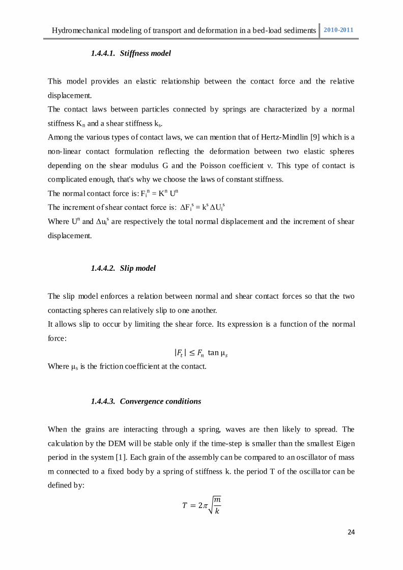
1.4.4.1. Stiffness model ................................................................................................. 24

1.4.4.2. Slip model ......................................................................................................... 24

1.4.4.3. Convergence conditions..................................................................................... 24

1.5. Software:......................................................................................................................... 25

1.6. Conclusion: ...................................................................................................................... 26

2.1. Introduction .................................................................................................................... 28

2.2. Different methods for the study of the solid fluid coupling ................................................. 28

2.3. Deformable pore-network modeling ................................................................................. 29

2.3.1. Volume decomposition using regular Delaunay triangulation ...................................... 29

2.3.2. Governing equations ................................................................................................. 31

2.3.2.1. Continuity ......................................................................................................... 31

2.3.2.2. Local conductance ............................................................................................. 32

2.3.2.3. Forces on particles ............................................................................................ 33

2.4. Conclusion ....................................................................................................................... 35

3.1. Introduction .................................................................................................................... 37

3.2. Modeling of Poiseuille flow............................................................................................... 37


5

3.3. Fixing the computation of “A” area ................................................................................... 38

3.4. Definition of Poiseuille flow rate ....................................................................................... 40

3.5. Parametric study .............................................................................................................. 41

3.5.1. Flow and number of grains ........................................................................................ 41

3.5.2. Flow and porosity ..................................................................................................... 41

3.5.3. Computation of the fluid forces on particles ............................................................... 42

3.5.4. Comparison with the analytical results ....................................................................... 43

3.5.5. Poiseuille flow for a disordered arrangement of particles ............................................ 45

3.6. Conclusion ....................................................................................................................... 47

4.1. Introduction:.................................................................................................................... 49

4.2. Viscous shear force formulation and implementation......................................................... 49

4.2.1. Shear stress expression ............................................................................................. 49

4.2.2. Determination of the interaction surface ................................................................... 50

4.3. Validation for a two sphere model .................................................................................... 52

4.4. Application to a bed sediment subjected to a shearing flow................................................ 54

4.4.1. Shields number......................................................................................................... 54

4.4.2. Evaluation of the critical Shields number .................................................................... 55

4.5. Conclusion ....................................................................................................................... 57

Conclusions and perspectives ...................................................................................................... 58

References.................................................................................................................................. 60


6

List of figures

Figure1.1: Poiseuille flow ........................................................................................................ 16

Figure 1.2: Shear plane (source: Andreotti et al (2011)). ......................................................... 18

Figure 1.3: (a) classification of the flow regimes as functions of I, (b) evolution of the contact

network as a function of I for a shear plane obtained by a 2D numerical simulation, lines

represent normal forces between particles (source Andreotti et al (2011)).............................. 19

Figure 1.4: Shear plane in an immersed granular material (source Andreotti et al (2011)) ..... 20

Figure 1.5: diagram of the different regimes as a function of (St, r) for an immersed granular

material (source Andreotti et al (2011)). .................................................................................. 21

Figure 1.6: Computation cycle in the DEM ............................................................................. 22

Figure 2.7: Regular Delaunay triangulation (a) and Voronoi diagrams (b). ............................ 29

Figure 2.8: Orientation of a cell. .............................................................................................. 30

Figure 2.9: Composition of a cell. ............................................................................................ 30

Figure 2.10: Pressure distribution on ij (a) in 2D and definition of facet spheres intersection

in 3D. ........................................................................................................................................ 33

Figure 3.11: Poiseuille flow model. ......................................................................................... 37

Figure 3.12: Delaunay triangulation problem. ......................................................................... 38

Figure 3.13: Distribution of areas to compute. ......................................................................... 39

Figure 3.14: S0 computation. ................................................................................................... 39

Figure 3.15: Q darcy and Q Poiseuille as functions of e. ......................................................... 40

Figure 3.16: Q=f(e) for various number of spheres. ................................................................. 41

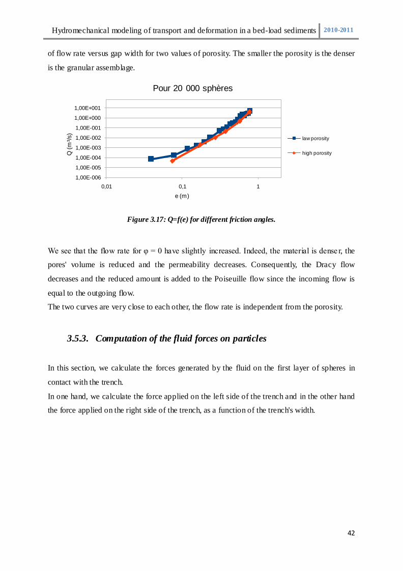
Figure 3.17: Q=f(e) for different friction angles. ..................................................................... 42

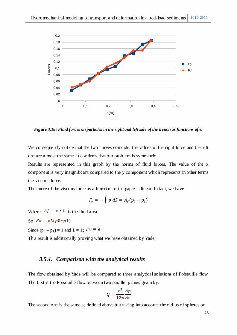
Figure 3.18: Fluid forces on particles in the right and left side of the trench as functions of e.

.................................................................................................................................................. 43

Figure 3.19: model of a regular mesh....................................................................................... 44

Figure 3.20: Q/Q* = f (e/L) for the different Poiseuille flows. ................................................ 45

Figure 3.21: : Poiseuille model with irregular surface in contact with the trench. ................... 46

Figure 3.22: Numerical and analytical flows as functions of e. ............................................... 46

Figure 3.23: Voronoi diagram at the trench. ............................................................................ 47

Figure 4.24: pore volume and solid area of spheres. ................................................................ 50

Figure 4.25: Interaction surface in three dimensions. .............................................................. 51

Figure 3.26: interaction surface S............................................................................................. 51


7

Figure 3.27: the scheme of a two sphere model. ...................................................................... 52

Figure 4.28: a bed load sediment model. .................................................................................. 54

Figure 4.29: Distribution of the Shields number corresponding to the onset of the grain

motion ....................................................................................................................................... 56

Figure 4.30: Evolution of kinetic energy as a function of viscous force. ................................. 56


8

List of tables

Table 1: Interaction surface for the different edges: ................................................................ 52

Table 2: Shearing viscous force for a two spheres model: ....................................................... 53


9

"To see a world in grain of sand,

And a heaven in a wild flower;

Hold infinity in the palm of your hand;

And eternity in an hour."

William Blake


10

General introduction

During the last years, the flow of granular material in presence of interstitial fluid have been

the subject of considerable researches combining inherent difficulties in granular material and

those within the world of suspensions. Particles flowing in fluid undergo both contact

interactions and hydrodynamic interactions. A lot of questions on the rheology of immersed

granular flows are still pending.

When the granular material is strongly agitated, it behaves as a dissipative gas. At slow

deformations, the quasi-static regime is described with plasticity theories. Between the two

regimes, the material flows like a liquid. Many experiments have been interested in

characterizing dense granular flows in different configurations; we focus our study in this

project in controlling the behavior of immersed granular flows in a laminar flow.

In the last few years, new numerical methods have been proposed. They are based on discrete

elements considering the soil as a discontinuous medium composed of grains in interaction.

This method allowed us to study the behavior of particles assembly subjected to a shearing

movement.

The present work is divided into four chapters:

Chapter 1 is devoted to the bibliography in which the most important bases of our project are

introduced. First we define granular materials and the two classical flows of the fluid

mechanics. Then, we talk about the rheology of granular flows. Finally, we present the

Discrete Element Method (DEM), its principle, the contact laws and the computation cycle of

a simulation in this method.

Chapter 2 is dedicated to introducing the solid fluid coupling model developed by E.Catalano,

a PhD student in the 3S-R Lab. It aims to calculate the viscous forces exerted on the solid

phase of particles.

Chapter 3 presents the study results of an immersed granular material subjected to a Poiseuille

flow. The purpose of this chapter is to compare and validate the simulated Poiseuille flow

with respect to theoretical Poiseuille flow.


11

Chapter 4 is devoted to the study of the shear in a granular material. A first part deals with the

implementation of a viscous force model for sheared particles. A second one is an application

to the determination of critical Shields number of immersed granular material under shearing

flow.


12

Presentation of the laboratories

Soil, Solid, Structures and Risk Lab:

The laboratory Soils, Solids, Structures – Risks, includes all the manpower in Grenoble

University on geomechanics, civil engineering and associated risks as well as mechanical and

multi physics coupling in solid media complex. It is a joint research unit (UMR 5521)

between CNRS (ST2I departments and EDD), the University Joseph Fourier and the “Institut

National Polytechnique de Grenoble”.

The aims of the lab include analysis and development of tools for optimization and the

vulnerability of structures and systems, in the field of environmental and technological risks

and in the field of mechanical behavior and conduct in-service. Researches in all these

domains are based on experiments developing new models which take into account the

physical-mechanical coupling and multi-scale analysis, therefore is equipped with original

and relevant experimental methods in mechanics of materials, geomaterials (soils, rocks,

concrete) and structures. Numerical modeling, leading to powerful tools, presents the most

important aim of all researches based on numerical technology advances (finite elements,

discrete elements, couplings...).

3S-R, directed by Mr Jacques Desrues, receives each year about fifty doctoral students. It

comprises five research teams:

- Geomaterials, Deformation and rupture (GDR): led by Pierre Bésuelle, a

researcher at CNRS.

- Géomécanique et Ouvrages (GéO): led by Fabrice Emeriault, professor at “l’Ecole

Nationale Supérieure pour l’Energie, l’Eau et l’Environnement » (ENSE3) in

l’INP de Grenoble (INPG).

- Mécanique et couplages multiphysiques des milieux hétérogènes (CoMHet), led by

Denis Favier, a professor at l’Université Joseph Fourier.

- Mécanique des matériaux solides et des milieux complexes (2MSMC) : led by

Didier Imbault, an associate professor at the University of Grenoble.

- Division of risks and vulnerabilities of structures: led by Yann Malécot, a

professor at University of Grenoble.

- Discrete Mechanics and Instabilities in Natural Materials (MeDiNa): led by Bruno

Chareyre, an associate Professor at the University of Grenoble.


13

LEGI lab:

LEGI, the laboratory of Geophysical and Industrial Flows, is a public research lab of the

University of Grenoble.it is a joint research unit (UMR 5519) common to the nat ional center

for scientific research (CNRS), University Joseph Fourrier (UJF) and Institut National

Polytechnique de Grenoble (Grenoble INP) which gathers more than 180 people, including 70

permanent and as many PhD students and postdocs.

LEGI lab focuses its researches on dynamics of turbulent flows, geophysical fluid dynamics

and flows with strong hydrodynamic coupling. These researches combine modeling, testing,

high performance numerical simulation and the development of innovative measuring

instruments. It has different resources and research facilities to conduct their projects on

various aspects of fluid mechanics (aerodynamics, cavitation, rotational flow, free surface

flows), both experimental (production flows) and numerical ones (modeling and simulation).

Directed by Cristophe Baudet, LEGI lab comprises seven researches teams:

- EDT team: Two-Phase flows and turbulence, headed by Jean Paul Thibault a

research officer.

- Energetics team, headed by Philippe Marty, a professor at Institut National

Polytechnique de Grenoble.

- ERES team: Environment, Rotation and Stratification, led by Chantal Staquet a

professor at Institut National Polytechnique de Grenoble.

- Houle team: Gravity Waves and Hydrodynamics Sedimentary, led by Hervé

Michallet a research officer.

- MIP team: Microfluidics, interfaces, Particles, led by Jean Luc Achard, a research

director.

- MEOM team: Ocean Modeling Flow Medium and Large Scale, led by Bernard

Barnier.

- Most team: Modelling and Simulation of Turbulence, led by Guillaume Balarac,

an associate professor at Institut National Polytechnique de Grenoble.


14

Chapter 1:

Bibliography


15

1.1. Introduction

The soil, a discontinuous medium, has always been assimilated and studied as a continuous

medium. The use of discrete element method is one of the new approaches developing the

discontinuous character of the soil. Indeed, the ground is no longer a continuous medium

whose behaviour is described throughout the elementary volume, but as a set of particles

interacting through contact forces. One of these methods is that of Cundall [16] which is

known for its reproduction of the complexities of soil behaviour through simple laws of

contact between grains.

In this chapter, we will define first the rheology of granular materials. We will then present

classical flow configurations that can be encountered in the theory of immersed granular

flows. Finally we will introduce the discrete element method.

1.2. Definitions

1.2.1. Granular material

We call “granular” a medium that is composed of a set of particles whose dimensions

exceed 100 µm [14]. Granular materials are found in many industrial sectors (structures

and civil engineering, chemical industry, pharmaceutical industry ...) and many

geophysical problems (rock avalanche, erosion, landslide, sediment transport...).

Characterization of the medium is based on the knowledge of the grain’s geometry (shape,

size, ...) and mechanical characteristics (density, stiffness, ...). Interstitial fluid is likely to

affect the behaviour of such material.

Studies carried out on granular materials revealed its behaviour’s complexity. Thus,

according to external conditions imposed on the medium, it may have a comparable set of

changes that of a solid, liquid or gas. Moreover, even in the case of apparent geometrical

homogeneity, a granular packing is inherently heterogeneous in terms of mechanical

stress. This property makes granular material extremely sensitive to disturbances.

A granular material has a set of pores which form a continuous network connected to the

exterior medium through which a fluid can flow and modify the behaviour of the system

as a whole.


16

1.2.2. Fluid mechanics

For the sake of simplicity and because flows in dense porous medium are characterized by

low Reynolds number, we will consider here laminar flow problems. In what follows, we

describe two classical laminar flows. The flow driven by a pressure gradient (Poiseuille flow)

and the flow driven by a moving plate at a constant velocity (Couette flow).

1.2.2.1. Poiseuille flow

The fluid is considered Newtonian and incompressible; its volume remains constant under the

action of external pressure. The fluid flows between two parallel planes whose equations are

y= L / 2 and y=- L / 2 (figure 1.1) [4]. A pressure gradient is applied in the x direction between

the two ends of the plans.

Figure1.1: Poiseuille flow

The mechanical equilibrium imposes:

𝜕

𝜕𝑧 𝜕𝑢

𝜕𝑧 +

𝜕𝑝

𝜕𝑥= 0

This equation is integrated twice to give:

𝑈𝑧 = 12𝜂𝜕𝑝

𝜕𝑥𝑧² + 𝑐𝑧 + 𝑑

With boundary conditions: u(L/2) = u(-L/2) = 0, we get c=0 and d= 1/2η ∂p/∂x L²/4 .


17

Thus velocity profile is given by the following formula:

𝑈𝑧 = 12𝜂𝜕𝑝

𝜕𝑥(𝑧2 −

𝐿2

4)

In a Poiseuille flow, velocity follows a parabolic profile with a maximum value of:

𝑈𝑚𝑎𝑥 = 18𝜂𝜕𝑝

𝜕𝑥𝐿²

Flow rate is then obtained from the integral of the velocity along the z direction, and we get:

𝑞 = −𝐿3

12𝜂

𝜕𝑝

𝜕𝑥

1.2.2.2. Couette flow

The fluid is again Newtonian and incompressible. The fluid flows between two parallel planes

whose equations are y= 0 and y = L, one is fixed and the other moves at a constant velocity

U0 [4]. Therefore no pressure gradient exists.

The mechanical equilibrium needs:

𝜕

𝜕𝑧

𝜕𝑢

𝜕𝑧 = 0

We integrate this equation twice and find:

𝑈𝑧 =𝑐

𝜂𝑧+ 𝑑

Boundary conditions: u(0)=0 then d=0

u(L)=U0 then c=U0 η / L

Thus the velocity profile is given by:

𝑈𝑧 =𝑈0𝜂

𝐿𝑧

In a Couette flow, the velocity profile is linear with z.

Flow rate is the integral of velocity along the direction z, and we find:

𝑞 =𝑈0𝜂𝐿

2


18

1.3. Rheology of dense granular flows

For four decades, the scientific community has tried to understand the macroscopic behavior

of flowing granular material. During the last decade, a phenomenological rheology of dense

granular flows has emerged. It was shown to capture the main characteristics of such flows.

Some open questions remains unanswered especially those covering localization and finite

size effects.

1.3.1. Dry granular flows

Let’s consider the shear flow represented in the figure 1.2. A set of spherical grains (diameter

d and density ) is confined between two rough planes with a pressure P applied on the top

plane moving with a velocity Vw. A velocity gradient 𝛾 =𝑉𝑤

𝐿 is imposed where L is the

distance between the two planes.

Figure 1.2: Shear plane (source: Andreotti et al (2011) [15]).

Numerical simulations using discrete element method (Da Cruz et al 2004; Iordanoff &

Khonsari 2004) suggest that this system of dense granular material is controlled by a single

dimensionless parameter called the inertial number [11]:

𝐼 =𝛾 𝑑

𝑃/

This parameter is the ratio between two time scales:

a microscopic time scale 𝑑/ 𝑃/𝜌: related to the confining pressure. It’s the


19

time that a particle requires to fall in a hole of size d under a pressure p.

a macroscopic time scale 1

𝛾 : related to the mean shear. It’s the time taken for a

particle to move and reach the grain below.

Depending on this parameter's value, there are three flow regimes [12]:

310

<I , the flow regime is quasi static (elasto-plastic material).

110

>I , collisional regime, the material is strongly agitated.

311010

<I< , dense flow regime.

I is the only parameter that characterizes rigid grains, the shear stress is, in fact, a function of

I:

𝜏 = 𝑃𝜇(𝐼)

Where μ is the effective friction coefficient.

This configuration gives then a relationship between the shear and normal stress with a

friction coefficient depending on I.

Figure 1.3: (a) classification of the flow regimes as functions of I, (b) evolution of the contact

network as a function of I for a shear plane obtained by a 2D numerical simulation, lines represent

normal forces between particles (source Andreotti et al (2011)[15]).


20

In order to move from quasi static to liquid and then gaseous regime, we have to increase the

shear rate or decrease the confining pressure. This transition between regimes is obvious

through the figure (1.3) showing the evolution of forces network as a function of I.

1.3.2. Immersed granular flow

Let’s consider the same configuration, but this time with grains immersed in fluid of viscosity

. In this case, particles are confined by a normal stress Pp imposed through a porous plate

allowing the fluid to flow (figure 1.4) [15]. The horizontal displacement of the plane

introduces a shear 𝛾 .

Figure 1.4: Shear plane in an immersed granular material (source Andreotti et al (2011) [15])

The analysis of the time tmacro defined for a dry flow, shows the existence of three regimes:

- Regime of free fall: the drag induced by fluid is insignificant, the regime is then the

same as for dry granular flows and 𝑡𝑚𝑖𝑐𝑟𝑜 = 𝑑/ 𝑃𝑝/𝜌𝑝

- Viscous regime: the velocity of the sphere is controlled by the equilibrium between the

drag force and the stress applied on the particle and 𝑡𝑚𝑖𝑐𝑟𝑜 = /𝑃𝑝.

- Turbulent regime: the velocity of the sphere is controlled by both the drag force and

the stress applied on particles. 𝑡𝑚𝑖𝑐𝑟𝑜 = 𝑑/ 𝑃𝑝/𝜌𝑝𝐶𝑑 where Cd is a drag coefficient.

The transition between these regimes is controlled by two dimensionless numbers as shown in

the figure 1.5:


21

Figure 1.5: diagram of the different regimes as a function of (St, r) for an immersed granular

material (source Andreotti et al (2011) [15]).

𝑆𝑡 =𝑡𝑚𝑖𝑐𝑟𝑜𝑓𝑟𝑒𝑒 𝑓𝑎𝑙𝑙

𝑡𝑚𝑖𝑐𝑟𝑜𝑣𝑖𝑠𝑐

=𝑑 𝑃𝑝𝜌𝑝

𝜂

𝑟 = 𝑡𝑚𝑖𝑐𝑟𝑜𝑓𝑟𝑒𝑒 𝑓𝑎𝑙𝑙

𝑡𝑚𝑖𝑐𝑟𝑜𝑡𝑢𝑟𝑏

2

=𝜌𝑝𝜌𝑓𝐶𝑑

1.4. Discrete element method (DEM)

1.4.1. Definition and principle of the DEM

The Discrete Element Method (DEM), known also as the distinct element method, is a multi-

scale approach using simple interaction laws for spherical particles whose movements are

governed by the fundamental principle of dynamics [1]. Proposed by Cundall in 1971, it

becomes the most widely used method for solving problems of discontinuous granular

materials, especially in granular flows and soil mechanics [5]. The behaviour of materials in

the DEM is governed by the contact laws between materials.

The DEM simulation consists in:

detecting collision between particles, creating new interactions and determining their

properties for two particles that can be interacted.

evaluating deformation, calculating the stresses and forces applied on particles for


22

already existing Interactions [2].

Detailed derivations and implementations may be found in [2].

1.4.2. Computing cycle

The computation cycle in the DEM is mainly characterised by two stages [6]: the first step

deals with the calculation of particles' positions, the second one is about contact forces.

Another step may be added, consisting on updating the list of contacts.

In fact, a list of current contacts is required to determine the shape, the position and the

orientation of particles. The procedures in place for that purpose can save time by elaborating

or making a list of potential contacts based on the division of the space with a grid, so that,

two particles are in contact if the distance between their centres is inferior to the sum of their

radii.

The normal and shear contact forces, are calculated separately, with the use of the interaction

law. We then deduce the torque effort applied on each particle.

The next step concerns the kinematic evolution of grains according to the law of motion

which will be presented in the following paragraph.

The computation cycle in the DEM is shown schematically in the figure 1.6:

Figure 1.6: Computation cycle in the DEM [6]


23

1.4.3. Laws of motion

The granular material is represented by a stack of spherica l particles. Each one is

characterised at time t by its position yi, linear velocity 𝑦𝑖 and angular velocity 𝑤𝑖 . Knowing

the positions of particles, we can find at any time a list of contacts for each particle and then

calculate the interaction forces between particles.

If we denote mp the mass of a particle and Ip its inertia, we can determine the acceleration in

translation and rotation according to the principle of dynamics [5]:

𝑦𝑖 =𝐹

𝑚𝑝

𝑤𝑖 =𝑀

𝐼 𝑝

Where {F,M} is the resultant torque of contact forces on particle.

Grains are moving during the simulation, so we denote their positions at each time step Δt.

We suppose that accelerations have already been calculated by successive integrations along a

centered finite difference scheme on a time step Δt, we obtain velocities at t + Δt/2 :

[𝑦𝑖 ]t+ Δt/2 = [yi]t- Δt/2 + [yi]t * Δt

[𝑤𝑖 ]t+ Δt /2 = [wi]t- Δt/2 + [wi]t * Δt

The new positions of particles at t + Δt are:

[yi]t+ Δt = [yi]t- + [yi]t+Δt/2 * Δt

[wi]t+ Δt = [wi]t- + [wi]t+Δt /2 * Δt

Contact forces are recalculated taking into account the new positions of particles.

All these interactions are performed to converge the system towards a state of static

equilibrium.

1.4.4. Contact laws

The contribution of the DEM is its ability to reproduce complex mechanical phenomena while

retaining a small number of mechanical parameters. To achieve this goal, it is necessary to

implement simple laws of interactions:


24

1.4.4.1. Stiffness model

This model provides an elastic relationship between the contact force and the relative

displacement.

The contact laws between particles connected by springs are characterized by a normal

stiffness Kn and a shear stiffness ks.

Among the various types of contact laws, we can mention that of Hertz-Mindlin [9] which is a

non- linear contact formulation reflecting the deformation between two elastic spheres

depending on the shear modulus G and the Poisson coefficient ν. This type of contact is

complicated enough, that's why we choose the laws of constant stiffness.

The normal contact force is: Fin = Kn Un

The increment of shear contact force is: ΔFis = ks ΔUi

s

Where Un and Δuis are respectively the total normal displacement and the increment of shear

displacement.

1.4.4.2. Slip model

The slip model enforces a relation between normal and shear contact forces so that the two

contacting spheres can relatively slip to one another.

It allows slip to occur by limiting the shear force. Its expression is a function of the normal

force:

𝐹𝑡 ≤ 𝐹𝑛 tan µ𝑠

Where μs is the friction coefficient at the contact.

1.4.4.3. Convergence conditions

When the grains are interacting through a spring, waves are then likely to spread. The

calculation by the DEM will be stable only if the time-step is smaller than the smallest Eigen

period in the system [1]. Each grain of the assembly can be compared to an oscillator of mass

m connected to a fixed body by a spring of stiffness k. the period T of the oscilla tor can be

defined by:

𝑇 = 2 𝑚

𝑘


25

We must use a time step large enough to describe this oscillation. A critical time step is set

automatically at the beginning of each cycle. We determine for each degree of freedom i the

equivalent contact stiffness Ki surrounding the element.

∆𝑐𝑟𝑖𝑡 = 𝑆 ∗min 𝑚𝑖

𝐾𝑖

Where S is the fraction of the smallest period obtained on all particles.

The DEM provides at each calculation cycle the dynamic equilibrium of the granular

assembly. The purpose is to reach a state of static equilibrium by mainta ining the principle of

the DEM. If the contact interactions are purely elastic, no energy is then dissipated. The

computer codes allow the introduction of a damping in the grain system called viscous or non

viscous.

Viscous damping is to connect each grain of the assembly by dampers working in translation

and rotation. This introduces energy dissipation at the interactions between the grains in

contact with shock absorbers.

Cundall has proposed a non-viscous damping that applies independently to each grain.

Damping force is then proportional to the resultant force on the grain.

1.5. Software:

Different computer codes are developed for DEM simulations. Some are commercial

software, like PFC [17], others are in-house codes developed in scientific institutions and a

few of them are distributed under open-source licenses like the software Yade.

Yade is an extensible open-source framework for discrete numerical models, based on

Discrete Element Method [2]. The project started as a result of SDEC at Grenoble University

and is nowadays developed in several research units. Yade use C++ for computation and

allows the implementation of new algorithms, the incorporation of interface with other

programs and operations of imports and exports data. Python can also be used to create and

manipulate the simulation. Details of this code can be in the appendix A.


26

1.6. Conclusion:

Basic knowledge required to understand this work have been presented in this chapter. The

study of shear in a dense granular flow is developed according to the DEM. For that purpose,

Yade will be used.


27

Chapter 2:

Solid fluid coupling


28

2.1. Introduction

This chapter concerns the presentation of the solid fluid coupling model [7] developed by

Emmanuele Catalano, a Phd student in the 3S-R lab. His work represents the first step in the

development of an efficient model for saturated granular material under stress, aiming at

determining the viscous forces applied on particles. We first review briefly the existing

methods for coupling discrete models with fluid flow. Next, we detail Catalano’s model.

2.2. Different methods for the study of the solid fluid coupling

Various methods have been presented in the literature in order to model the solid fluid

coupling. They differ in the decomposition of the pore volume.

- Microscale Stokes flow modeling: the numerical Stokes solution is reflecting in details

complex three-dimensional pore geometries which uses the Finite Element Method,

finite volumes, Lattice Boltzmann and other methods.

- Continuum-discrete Darcy flow modeling: this approach uses the coarse-grid CFD

methods where the flow and the solid-fluid interactions are defined with simplified

semi-empirical models based on Darcy law. Despite its performance in making

coupled problems affordable in terms of CPU cost, this method cannot be efficient in

solving some problems like segregating phenomena, internal erosion by transport of

fines,…

- Pore-network modeling: this approach was developed to predict the permeability of

materials from microstructual geometry using a simplified representation of porous

media. It was a well-known strategy for its appropriate definition of how fluids are

distributed between pores. Usually, it’s used with undeformable solid skeleton.

- Deformable pore-network modeling: this approach had focused its studies in

developing expressions of forces applied on solid particles in the aim to be used in

three-Dimensional DEM simulations. This solution was limited to 2D models of discs

assemblies, it has been adapted to 3D assemblies in the work of Catalano.


29

2.3. Deformable pore-network modeling

2.3.1. Volume decomposition using regular Delaunay triangulation

Delaunay triangulation (figure 2.7.a) and the Voronoi graph (figure 2.7.b) are used for

structural study of molecules, liquids and granular materials. The most used Delaunay model

is defined for a set of points. The graph of Voronoi defines, in this case, polyhedra around

each point and facets of the polyhedra are equidistant to two adjacent points.

Figure 2.7: Regular Delaunay triangulation (a) and Voronoi diagrams (b).

The Computational Geometry Algorithms Library CGAL, an Open Source Project, is the library used

to access to efficient geometric algorithms in the form of a C++ library and define the Regular

Delaunay triangulation and Voronoi graph. [13].

The triangulation is a set of points called vertices and a collection of cells linked together through

incidence relations.

Each cell gives access to its four incident vertices and adjacent cells. However, each vertex gives

access to one of its incident cells.

The vertices of each cell are indexed with 0, 1, 2 and 3 in positive orientation, the neighbors too , such

the way that the neighbor indexed by i is opposite to the vertex i.


30

Figure 2.8: Orientation of a cell [13].

Figure 2.9: Composition of a cell [13].

The Voronoi cells S are often used. They define the split between the spheres as curved

surfaces equidistant from both spheres surfaces. But using this type of grap h is

computationally costly for surfaces and volumes. To avoid this problem, regular Delaunay

triangulation was then proposed. It uses weighted points where weights account for the radius

of the spheres. The Voronoi graph is then entirely contained in the voids between the spheres,

which is not possible for the classical Delaunay triangulation. Edges and facets of the regular

Voronoi graph are lines and planes enabling a quick and easy computation of geometrical

quantities.

In what follows, we will use the combination of facets of the regular Delaunay triangulation

and vertices of the regular Voronoi graphs, in order to decompose the voids volume.

Ω: domain occupied by a porous material will be decomposed to:

Γ: domain occupied by solid.

Θ: domain occupied by fluid.


31

Nc is the number of tetrahedral cells in the regular Delaunay triangulation of the spheres

packing.

Ωi is the domain defined by the tetrahedron I.

We have: Ω = Ωi𝑁𝑐1

We define Ns as the number of spheres and Γi as the domain occupied by the sphere i.

We have Γ = Γ𝑖𝑁𝑠1

2.3.2. Governing equations

2.3.2.1. Continuity

We define Θi as the part of the tetrahedron Ωi occupied by fluid, its volume is Vif.

The continuity equation of an incompressible fluid is:

𝑉𝑖𝑓 = 𝑣 − 𝑢 𝑛 𝑑𝑆

𝜕𝜃 𝑖

Where 𝜕𝜃𝑖 the contour of the domain 𝜃𝑖 and n is the outward pointing unit vector normal to

𝜕𝜃𝑖 .

u is the fluid velocity and v is the contour velocity.

We define 𝜕𝑠 𝜃𝑖 as the solid-fluid interface where we have: (v – u) n = 0. So the integration

can be restricted to 𝜕𝑓 𝜃𝑖 , the fluid interface.

We introduce 𝑆𝑖𝑗𝑓

(𝑗 ∈ 𝑗1, 𝑗2, 𝑗3 , 𝑗4 ) the intersections of triangular surfaces Sij with the fluid

domain, so that, 𝜕𝑓 𝜃𝑖 = 𝑆𝑖𝑗𝑓𝑗4

𝑗1 , we can define the fluid flux from tetrahedron I to adjacent

tetrahedra j1 to j4 :

𝑉𝑖𝑓 = 𝑣− 𝑢 𝑛 𝑑𝑆 = − 𝑞𝑖𝑗

𝑗4

𝑗1𝑆𝑖𝑗𝑓

𝑗4

𝑗1


32

The volume 𝑉𝑖𝑓 is constant since we supposed that particles are fixed. So the continuity

equation is simplified to:

𝑞𝑖𝑗 = 0

𝑗4

𝑗1

2.3.2.2. Local conductance

The domain Ω is defined as a set of subdomains Ω𝑖𝑗 , the union of two tetrahedra constructed

from facet 𝑆𝑖𝑗 and Voronoi vertices Pi and Pj and Θij is a throat connecting two pores. Its

length is 𝐿𝑖𝑗 = 𝑃𝑖 − 𝑃𝑗

Φij is the volume of Θij and γij is the surface of Θijs

, the part of the contour in contact with

spheres.

The hydraulic radius is defined as follows:

𝑅𝑖𝑗𝑕 =

𝜙𝑖𝑗𝛾𝑖𝑗

So that we have:

𝑞𝑖𝑗 = 𝑔𝑖𝑗 𝑝𝑖 −𝑝𝑗

𝐿𝑖𝑗

𝑔𝑖𝑗 = 𝜒𝐴𝑖𝑗 𝑅𝑖𝑗

𝑕 ²

𝜇

gij is the local conductance of the facet ij and pi – pj is the pressure difference between two

connected tetrahedral cells.

is a shape factor taken equal to 2π, by analogy with the Hagen-Poiseuille law for cylindrical

tubes.


33

2.3.2.3. Forces on particles

The force applied on the particle k by fluid is decomposed in two terms:

Fp,k , the pressure stress on the contour ij

Γ .

Fv,k , the viscous stress on the contour ij

Γ .

𝐹𝑘 = 𝑝𝑛 + 𝜏𝑛 𝑑𝑆 = 𝑝𝑛 𝑑𝑆 + 𝜏𝑛 𝑑𝑆 =𝜕Γij𝜕Γij𝜕 Γij

𝐹𝑝 ,𝑘 + 𝐹𝑣,𝑘

Figure 2.10: Pressure distribution on ij (a) in 2D and definition of facet spheres intersection in

3D. [7]

Pressure stress

The force generated by pressure on particle k in the domain Ωij is the sum of two terms pi and

pj.

𝐹𝑖𝑗𝑝 ,𝑘

= 𝑝𝑖𝜕Γ𝑖𝑗 ∩𝜕Ωij

𝑛 𝑑𝑆 + 𝑝𝑗𝜕Γ𝑖𝑗 ∩𝜕Ωij

𝑛 𝑑𝑆

In the domain Ωij, the pressure stress is proportional to the areakij

kΓS=Aij . Noting that

nij is the unit vector pointing from Pi to Pj , the pressure force is then:

𝐹𝑖𝑗𝑝 ,𝑘 = 𝐴𝑖𝑗

𝑘 (𝑝𝑖 −𝑝𝑗 )𝑛𝑖𝑗


34

Viscous stress

The integration of the total viscous stress applied on the solid phase in Ωij gives a total

viscous force:

𝐹𝑖𝑗𝑣 = 𝜏𝑛 𝑑𝑆

𝜕𝜃𝑖𝑗𝑠

Using the divergence theorem, we obtain:

(𝑝𝑛 + 𝜏𝑛) 𝑑𝑆 = 0𝜕𝜃𝑖𝑗

Or:

𝜏𝑛 𝑑𝑆 + 𝜏𝑛 𝑑𝑆 + 𝑝𝑛 𝑑𝑆 = 0𝜕𝜃𝑖𝑗𝜕𝑓𝜃𝑖𝑗

𝜕𝑠𝜃𝑖𝑗

If we suppose that pressure gradients are equilibrated by viscous stress on the solid phase

only, thus neglecting the term 𝜏𝑛 𝑑𝑆𝜕𝑓𝜃𝑖𝑗

gives:

𝐹𝑖𝑗𝑣 = − 𝑝𝑛 𝑑𝑆 = 𝐴𝑖𝑗

𝑓 (𝑝𝑖 −𝑝𝑗 )𝑛𝑖𝑗 𝜕𝜃𝑖𝑗

In order to express the viscous force applied on each of the three spheres in Θij, we consider

that the force on a sphere is proportional to the surface of the sphere contained in the

subdomain. Then:

𝐹𝑖𝑗𝑣,𝑘 = 𝐹𝑖𝑗

𝑣 𝛾𝑖𝑗𝑘

𝛾𝑖𝑗𝑘3

1


35

2.4. Conclusion

We have defined in this part of the report the viscous force applied on the solid phase of

particles by means of the regular Delaunay triangulation.

These forces were determined by neglecting the viscous stress applied on fluid-fluid parts of

the interfaces between volume elements. As a consequence, the model can’t give correct

estimates of viscous forces generated by shear deformation. This will be one of the inputs of

the present work.


36

Chapter 3:

Poiseuille flow test case


37

3.1. Introduction

In this chapter the response of the model in a Poiseuille- like configuration will be studied.

The numerical model generated by Yade represents a packing of spheres in which is entailed a

Poiseuille flow. The results will be compared with the analytical solutions in order to validate

our computational model.

Two types of interactions are present in this model: sphere- sphere interaction and fluid-

sphere interaction. We are interested in our study in controlling grains’ behavior in presence of

fluid and calculating forces generated on particles.

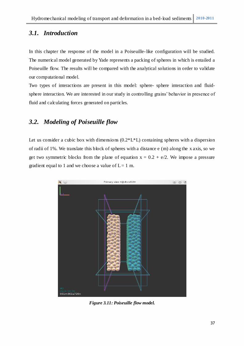
3.2. Modeling of Poiseuille flow

Let us consider a cubic box with dimensions (0.2*L*L) containing spheres with a dispersion

of radii of 1%. We translate this block of spheres with a distance e (m) along the x axis, so we

get two symmetric blocks from the plane of equation x = 0.2 + e/2. We impose a pressure

gradient equal to 1 and we choose a value of L = 1 m.

Figure 3.11: Poiseuille flow model.


38

We recall that, by analogy with the Poiseuille's formula for a cylindrical tube, we define a

parameter called the hydraulic conductance as:

𝑔 =𝑅𝑕

2𝐴

Where Rh is the hydraulic radii, A is the fluid area, Χ is the shape coefficient and is the

viscosity.

The expression of the flow rate is then:

3.3. Fixing the computation of “A” area

By performing the computation of the flow rate, we initially found unexpected discrepancies

in results; there are areas that give us infinite values of permeability and flow rate. Careful

review of the code revealed that it was due to a special case in the decomposition of the

volume by the method of Delaunay triangulation that was not treated correctly in the original

code. We detail here how we find this problem.

Obtained triangles linking, as was already mentioned, the centers of the spheres, at most, one

facet of each triangle could cut the solid surface of a sphere belonging to the same triangle

(figure 3.11). The surface of the triangle would be smaller than the sum of solid surfaces in

contact with the fluid, giving consequently a negative value of the fluid surface, which is

physically impossible.

Figure 3.12: Delaunay triangulation problem.


39

To overcome this problem, we must take into account the solid surface that does not belong to

the triangle on which we make the computation of permeability.

Figure 3.13: Distribution of areas to compute.

We calculate the surface S0, the part of the sphere that doesn’t belong to the triangle and

would be subtracted from the calculation of the fluid area.

Figure 3.14: S0 computation.

𝑆0 = 𝑆1 − 𝑆2

𝑆1 = 0.5 𝑅²𝜃

𝑆2 = 0.5 𝑚 𝑑

Where:

𝑚 = 𝐵𝐴 ∧ 𝐵𝐶

𝐵𝐶 the distance of the sphere A from the opposite facet BC.

𝑑 = 2 𝑅0²− 𝑚²

= 2 𝑐𝑜𝑠−1 𝑚

𝑅0


40

3.4. Definition of Poiseuille flow rate

Once the fluid area is correctly computed, we can calculate the flow which is actually the sum

of two flows: the Poiseuille flow generated through the trench (zone between the two blocks

of spheres separated by the gap e) and the Darcy flow through the pores between grains:

Where k is the permeability which corresponds to e = 0.

𝐴′ = 0.2 ∗ 𝐿

For a packing of 20 000 spheres, we have calculated the average Poiseuille flow for different

values of e (figure 3.5).

Figure 3.15: Q darcy and Q Poiseuille as functions of e.

As we can see, the Darcy flow is very small, negligible compared to Poiseuille flow. This can

be explained by the difference of permeabilities which is a function of area (pore's area is very

small compared to the trench's one).

We can then consider that the flow rate generated by Yade is approximately equal to the

Poiseuille flow rate.

0,00E+00

5,00E-01

1,00E+00

1,50E+00

2,00E+00

2,50E+00

3,00E+00

3,50E+00

4,00E+00

4,50E+00

5,00E+00

0 0,2 0,4 0,6 0,8 1

Q darcy

Qpoiseuille


41

3.5. Parametric study

We study here the properties of the numerical flow rate for the already described model with a

smooth plane surface in contact with the fluid in the trench in order to be comparable with the

theoretical plane Poiseuille. We will show at the end the difference in terms of the flow rate

between considering a smooth and a rough surface by presenting some obtained results.

3.5.1. Flow and number of grains

In this section, we will calculate the flow rate through this configuration as a function of e for

various numbers of spheres.

Figure 3.16: Q=f(e) for various number of spheres.

In figure 3.15, we have presented the variation of the flow rate as a function of the trench's

width for various number of spheres (from 1 000 to 100 000 spheres). We can clearly see that

the curves Q=f (e) are very close one to the other. We can conclude then that the flow is

independent from the number of spheres.

3.5.2. Flow and porosity

In this section, we are interested in the influence of porosity which is controlled by the friction

angle defined as an intrinsic characteristic of the material. Figure 3.16 shows the comparison

1E-05

0,0001

0,001

0,01

0,1

1

0,01 0,1 1

Q (

m³/

s)

e (m)

Q (20 000)

Q (10 000)


42

of flow rate versus gap width for two values of porosity. The smaller the porosity is the denser

is the granular assemblage.

Figure 3.17: Q=f(e) for different friction angles.

We see that the flow rate for φ = 0 have slightly increased. Indeed, the material is dense r, the

pores' volume is reduced and the permeability decreases. Consequently, the Dracy flow

decreases and the reduced amount is added to the Poiseuille flow since the incoming flow is

equal to the outgoing flow.

The two curves are very close to each other, the flow rate is independent from the porosity.

3.5.3. Computation of the fluid forces on particles

In this section, we calculate the forces generated by the fluid on the first layer of spheres in

contact with the trench.

In one hand, we calculate the force applied on the left side of the trench and in the other hand

the force applied on the right side of the trench, as a function of the trench's width.

1,00E-006

1,00E-005

1,00E-004

1,00E-003

1,00E-002

1,00E-001

1,00E+000

1,00E+001

0,01 0,1 1

Q (

m³/

s)

e (m)

Pour 20 000 sphères

law porosity

high porosity


43

Figure 3.18: Fluid forces on particles in the right and left side of the trench as functions of e.

We consequently notice that the two curves coincide; the values of the right force and the left

one are almost the same. It confirms that our problem is symmetric.

Results are represented in this graph by the norms of fluid forces. The value of the x

component is very insignificant compared to the y component which represents in other terms

the viscous force.

The curve of the viscous force as a function of the gap e is linear. In fact, we have:

𝐹𝑣 = − 𝑝 𝑑𝑆 = 𝐴𝑓(𝑝0 − 𝑝1)

Where is the fluid area.

So

Since (p0 – p1) = 1 and L = 1;

This result is additionally proving what we have obtained by Yade.

3.5.4. Comparison with the analytical results

The flow obtained by Yade will be compared to three analytical solutions of Poiseuille flow.

The first is the Poiseuille flow between two parallel planes given by:

The second one is the same as defined above but taking into account the radius of spheres on

0

0,02

0,04

0,06

0,08

0,1

0,12

0,14

0,16

0,18

0,2

0 0,1 0,2 0,3 0,4 0,5

Fo

rce

s

e(m)

Fg

Fd


44

both sides of the trench. This means that:

𝑄 =𝑕3

12𝑛

∆𝑝

∆𝑧

Where h = e + 2 r.

The third one is that calculated for a regular mesh as shown in figure 3.18:

Figure 3.19: model of a regular mesh.

Let’s calculate the permeability K for one cell.

𝐾 =𝐴𝑓 𝑅𝑕

2

2

𝑅𝑕 =𝑉𝑣𝑆𝑠

=𝑕 2𝑟 2 − 4/3𝜋𝑟3

2𝜋𝑟²=𝑕

𝜋−𝑟

3

𝐴𝑓 = 𝑟𝑕 −𝜋𝑟2

2

The flow rate generated by the model is then:

𝑄𝑇 = 2𝑁 𝐾 Δ𝑃

𝑁𝐷

Figure 3.19 shows the evolution of Q/Q* = f (e/L) where Q is the flow rate and Q* is:

𝑄∗ = ∆𝑝 𝐿3/𝜂


45

Figure 3.20: Q/Q* = f (e/L) for the different Poiseuille flows.

We notice that for small values of e, the asymptotic behavior result of the numerical flow rate

is close to the regular Poiseuille one. For large values of e, the numerical flow rate diverges

from the regular Poiseuille solution because particles are no longer seen by the fluid in the

trench in terms of Voronoi graphs.

The two curves for plane Poiseuille Q= f(e) and Q= f(h) coincide for large values of e. This

can be explained by the fact that the larger the gap width is, the more the radius r is negligible

and the more h approaches to e.

3.5.5. Poiseuille flow for a disordered arrangement of particles

Let’s consider a cubic box with dimensions (L*L*L) containing spheres with a dispersion of

radii of 1%. We design an area e (m) wide where no sphere should exist, so that the two

blocks of the spheres placed on both sides of this area play the role of two parallel planes of

equations x = L/2 and x = - L/2.

We impose a pressure gradient equal to 1 and we choose a value of L = 1 m.


46

Figure 3.21: : Poiseuille model with irregular surface in contact with the trench.

We compare the flow rate generated by Yade to theoretical values of Poiseuille flow

calculated from the formula below:

Figure 3.22: Numerical and analytical flows as functions of e.


47

We notice that the values of Qyade are slightly larger than those of theoretical Poiseuille.

Comparing Qyade with the numerical flow calculated in the previous section for an idealized

configuration, we find that

This is caused by the fact that the surface of all spheres in contact with fluid is not quite

regular and spheres are not perfectly aligned as we can see in the graph below which shows us

the Voronoi graph.

Figure 3.23: Voronoi diagram at the trench.

This graph shows us the Voronoi diagram (with blue lines) and the width e of the trench that

has been created. We can clearly see that the fluid surface limited by Voronoi diagrams is

slightly larger than that limited by the trench. So, the flow would be undoubtedly larger than

the analytical flow.

3.6. Conclusion

The flow rate generated by Yade is in agreement with the analytical Poiseuille flow rate.

Moreover, we have checked that this flow rate is independent of the geometrical and

mechanical properties of the grains.


48

Chapter 4:

Modeling of shear in a Couette flow


49

4.1. Introduction:

When a bed of particles is subjected to a shearing flow, the particles on the surface can be set

in motion. This is linked with many problems of sediments transport and an active area of

research. That's why we will be interested in this chapter in the derivation of expressions for

the viscous forces generated in such case.

First, we will define the viscous shear force as functions of shear deformation at the particles

scale. Next, we will simulate the evolution of bed sediment under the effect of a shearing flow

and analyze the results in terms of shields number.

4.2. Viscous shear force formulation and implementation

The shearing viscous force is given by the formula below. It is the product of the shear stress

and the surface on which this stress is applied.

𝐹 = 𝜏 𝑆

4.2.1. Shear stress expression

The shear stress is obtained from dimensional consideration as a velocity difference between

two neighboring particles times the fluid viscosity, divided by a characteristic distance

between the two particles.

𝜏 =∆𝑉𝑡

𝑅𝑕

Where

- is the viscosity.

- ΔVt is the tangential component of the relative velocity of the two spheres.

∆𝑉𝑡 = 𝑉1 −𝑉2 − 𝑉1 −𝑉2 ∗ 𝑛 ∗ 𝑛

(V1 and V2 are the velocities of the two spheres)


50

- Rh is the hydraulic radius defined as:

𝑅𝑕 =𝑉𝑣𝑆𝑠

Vv is the pore volume and Ss is the solid area of spheres in contact with fluid (figure

4.23).

Figure 4.24: pore volume and solid area of spheres.

A simplified expression of the hydraulic radius was developed and used in the computation of

the viscous force:

𝑅𝑕 = 𝑑 + 0.45𝑅

Where d is the interparticular distance and R is the mean radius of spheres.

4.2.2. Determination of the interaction surface

S is the surface of interaction between two spheres (figure 4.24). It is defined as the area of

the polygonal facet separating the spheres in the Voronoi’s graph.


51

Figure 4.25: Interaction surface in three dimensions.

This area is the sum of triangles’ area composing the polygon (figure 3.25).

The algorithm iterates on all triangles by incrementing vertices v1 and v2.

Figure 3.26: interaction surface S.

Vertices v0, v1 and v2 represent the centres of neighbouring tetrahedral cells to which the edge

belongs.

The whole algorithm and functions corresponding to the computation of the shearing viscous

force are coloured in blue in the code files presented in the appendix B.


52

4.3. Validation for a two sphere model

In order to verify our algorithm, we generate a model of 6 walls and two spheres of radius 0.2 m in

contact.

Figure 3.27: the scheme of a two sphere model.

The results of the area calculated by Yade are shown in table 2.

Body 1 Body 2 S (m²)

sphere 1 wall 3 0,16





sphere 2 Sphere 1 0,159






Table 1: Interaction surface for the different edges:


53

If we compare these results to the analytical ones, we can confirm the adequacy of the

method, because the interaction surface between two bodies (sphere and sphere or sphere and

wall) is a square whose area is equal to 4R² = 0.16 m² (R is the radius of the sphere).

Since the interaction surface is correct, we can check the shear stress expression defined by

the equation ()

Body 1 Body 2 Viscous force (N)

sphere 1 wall 3 (0,0,0)





sphere 2 Sphere 1 (0,1.77,0)

sphere 2 wall 2 (0.00017,0,0)

sphere 2 wall 5 (0,1.77,0)

sphere 2 wall 1 (0,1.77,0)

sphere 2 wall 3 (0.00017,0,0)

sphere 2 wall 4 (0,1.77,0)

For all edges connecting a wall to the fixed sphere, the shearing viscous force is zero. When

we talk about the edge connecting the two spheres (one is fixed and the other moves with a

velocity U = (0, 1, 0)), this force becomes equal to:

𝐹 =𝑢 − 𝑢𝑛𝑅𝑕

∗ ∗ 𝑆 = 1.77 𝑁

Where S = 0.16 m², Rh = 0.09 m and = 1.

The viscous shearing force has been validated for the simplest system of two spheres moving

relatively.

We can now test our model in the more complex configuration of a set of spheres deposited in

a shear flow under gravity.

Table 2: Shearing viscous force for a two spheres model:


54

4.4. Application to a bed sediment subjected to a shearing flow

In order to study bed load transport, we prepare a sediment bed from an initial sedimentation

of a suspension under the gravity effect in a quiescent fluid (figure 4.27). A constant velocity

along the x direction is imposed as boundary condition on the top side of the domain. Particles

begin to move under the influence of two factors: the gravity and a drag force exerted by the

fluid on grains.

Figure 4.28: a bed load sediment model.

4.4.1. Shields number

For low fluid velocity, particles don’t move. There is so a threshold at which grains begin to

be transported by the fluid. In 1936, Shields has introduced a dimensionless number that

characterizes the motion threshold.

𝜃 =

𝜌𝑝 −𝜌𝑓 𝑔𝑑


55

Where:

d is the diameter of the grain.

g the gravitational acceleration.

is the bed shear stress.

p is the density of the particle.

f is the density of the fluid.

It’s the ratio between the hydro mechanical force or the drag force (d²) and the apparent weight of a

single particle ((p - f) g d3).

When the drag force tends to put grains in motion, the weight resists to this. The Shields number

controls then the stability of the particles :

- < c: No motion.

- > c: particles are in motion.

c is the critical Shields number from which particles start moving.

𝜃𝑐 =𝜏𝑐

𝜌𝑝 − 𝜌𝑓 𝑔𝑑

Experimental measurements show that the critical Shields number for the onset of particle motion is

set to 0.12 ± 0.03 for low Reynolds number. In the following simulations, he will be in the range 10-1

-

10-2

.

4.4.2. Evaluation of the critical Shields number

In order to evaluate the critical Shields number, we impose a variable velocity on the top wall.

As soon as particles begin to move, we calculate the viscous force applied on each grain and

the corresponding Shields number.

The distribution of the Shields number is represented in figure 4.28. We can see that the mean

critical Shields number is equal to 0.13 which is in agreement with the experimental results.


56

Figure 4.29: Distribution of the Shields number corresponding to the onset of the grain motion

If we look now to the evolution of the kinetic energy as a function of the viscous force, we set

out the graph represented in the figure (4.29).

Figure 4.30: Evolution of kinetic energy as a function of viscous force.


57

Kinetic energy is very small (about 10-8) for small values of viscous force; particles remain at

rest. From a viscous force equal to about 1,3 N, kinetic energy increases and particles begin to

move. This value of viscous force corresponds to a Shields number equal to 0,12.

4.5. Conclusion

According to the DEM, we were be able to study and control the motion of particles subjected

to a shearing flow. We have validated the results obtained by experimental measurements by

evaluating the critical Shields number. In fact, In a laminar flow, the onset of grain motion is

characterised by a critical Shields number equal to 0,12 ± 0,03 for small Reynolds number

(Re < 1).


58

Conclusions and perspectives

The purpose of this work concerns the behaviour of immersed grains subjected to a shearing

flow. This report has been divided into four main sections:

The first section recalled some basics of fluid mechanics and granular flow. It introduced to

the Discrete Element Method which is a very efficient method for studying the different

interactions in a granular material.

The second section presented the solid fluid coupling model developed in the 3SR lab and

based on the Delaunay triangulation method. It was our starting po int to study the shear

behaviour of saturated granular materials.

Before starting our study of the shear in a granular material, we have begun in the third

section with a simple model of Poiseuille flow where particles were fixed. We calculated the

flow rate generated by Yade and compared it with the analytical results. Numerical and

theoretical results are in agreement; the flow rate is independent of the geometric and

mechanical properties of particles subjected to a Poiseuille flow, and depends only on the

thickness of the gap between the two rigid blocks.

Finally, in the forth section, we derive a model of viscous force in sheared granular materials,

in the framework of Catalano's DEM-PFV model (original Catalano's model accouonting only

for volumetric deformations). This model has been implemented in Yade , then used to define

the viscous shear forces exerted on particles in simulations of granular bed under tangential

flow. The results have been analysed to determine the motion threshold defined by the so-

called dimensionless Shields number . The critical Shields number calculated numerically

corresponds to the results given by experimental measurements: in a laminar flow, particles

begin to be transported by the fluid for a critical Shields number equal to 0,12 ± 0,03.

As a conclusion, the DEM was a very promising method to study the behaviour of sheared

saturated granular media. This method is becoming increasingly popular although it is

relatively marginal compared to the Finite Element Method. This is because of the huge

computational time it requires for large sized simulations, but results obtained with this

method justify the effort it involves. We were able to elaborate and implement a model of

viscous forces due to shear deformation, as a complement to Catalano's volumetric effects.


59

The study of rehology of an immersed granular material has been performed for an

incompressible fluid through a totally saturated material and gave promising results. We

didn't take into account the compressibility of the fluid however. For this reason, a PhD thesis

is suggested in the 3S-R lab starting from the academic year 2011-2012 in which the tri-

phased problems will be studied using the Discrete Element method, in the aim of developing

a first and unique micro-hydro-mechanical coupling model in the three dimensional models.


60

References

[1] B.Chareyre, P.Villard; Dynamic Spar Elements and Discrete Element Methods in Two Dimensions

for the Modeling of Soil-Inclusion Problems; J. Engrg. Mech. 131 (10 pages) – 2005.

[2] V. Šmilauer, E. Catalano, B. Chareyre, S. Dorofeenko, J. Duriez, A. Gladky, J. Kozicki, C.

Modenese, L. Scholtès, L. Sibille, J. Stránský, K. Thoeni, Yade Documentation. The Yade Project -

2010.

[4] E. Guyon, J P. Hulin, L. Petit ; Hydrodynamique physique; EDP Sciences, CNRS éditions – 2001.

[5] B. Chareyre ; Modélisation du comportement d’ouvrages composites sol-géosynthétique par

éléments discrets, PhD Thesis Université de Grenoble I Joseph Fourrier – 2003.

[6] L. Sibille ; Modélisations discrètes de la rupture dans les milieux granulaires ; PhD Thesis, Institut

National Polytechnique de Grenoble – 2006.

[7] B. Chareyre, A. Cortis, E. Catalano, E. Barthélémy; Pore-scale modeling of viscous flow and

induced forces in dense sphere packings; submitted, Transport in porous media - 2011.

[8] V. Smilauer; Cohesive particle Model using the Dicrete Element Method on the Yade Platform,

PhD thesis - 2010.

[9] PFC3D Manual; Contact constitutive models: theory and backgrounds (PFC3D)

[10] D. Muller ; Techniques informatiques efficaces pour la simulation des milieux granulaires par

des méthodes d'éléments distincts ; PhD thesis ; Ecole Polytechnique Fédérale de Lausanne – 1996.

[11] Y. Forterre, O. Pouliquen; Flows of dense granular media – The annual review of fluid

mechanics Vol. 40: 1-24 – 2008.

[12] F. Chevoir, J N. Roux, F. Da Cruz, P. Rognon, G.Coval ; Lois de frottement dans les écoulements

granulaires denses ; LMSGC Institut Navier.

[13] J.-D.Boissonnat, O.Devillers, S.Pion, M.Teillaud, M.Yvinec. Triangulations in CGAL.

Computational Geometry : Theory and Applications, 22:5-19, 2002.

[14] O. Pouliquen ; Milieux granulaires ; CNRS Editions - 2001.

[15] B. Andreotti, Y. Forterre , O. Poulisquen ; Les milieux granulaires, entre fluide et solide ; CNRS

Editions – 2011.


61

[16] P.Cundall and O.Strack. A discrete numerical model for granular assemblies. Géotechnique,

(29):47-65, 1979.

[17] ICG (2003), Pfc3d (particle flow code in 3d) theory and background manual, version 3.0. Itasca

Consulting Group.

Date post:	07-Nov-2019
Category:	Documents
Upload:	others
View:	7 times
Download:	0 times

Hydromechanical modeling of transport and deformation in a...

Documents