560
8/9/2019 Hydrostatic Lubrication 1992
http://slidepdf.com/reader/full/hydrostatic-lubrication-1992 1/558

8/9/2019 Hydrostatic Lubrication 1992
http://slidepdf.com/reader/full/hydrostatic-lubrication-1992 2/558
HYDROSTATIC LUBR
I
CAT10N

8/9/2019 Hydrostatic Lubrication 1992
http://slidepdf.com/reader/full/hydrostatic-lubrication-1992 3/558
TRIBOLOGY SERIES
Advisory Board
W.J. Bartz (Germany, F.R.G.)
R. Bassani (I taly)
B. Briscoe (Gt. Britain)
H. Czichos (Germany, F.R.G.)
D. Dowson (Gt. Britain)
K. Friedrich (Germany, F.R.G.)
N. Gane (Australia)
W.A. Glaeser (U.S.A.)
M. Godet (France)
H.E. Hintermann (Switzerland)
K.C. Ludema (U.S.A.)
T. Sakurai {Japan)
W.O. Winer (U.S.A.)
Vol.
1
Vol. 2
Vol. 3
V O l .
4
V O l . 5
Vol. 6
Vol.
7
Vol.
8
VO l . 9
VO l . 10
VOl.
11
VOl. 12
Vol.
13
Vol. 14
Vol. 15
Vol.
16
Vol. 17
Vol. 18
VOl. 19
VOl. 20
Vol. 21
VO l . 22
Tribology - A Systems Approach to the Science and Technology
of Friction, Lubrication and Wear (Czichos)
Impact Wear of Materials (Engel)
Tribology of Natural and Artificial Joints (Dumbleton)
Tribology of Thin Layers (Iliuc)
Surface Effects in Adhesion, Friction, Wear, and Lubrication (Buckley)
Frict ion and Wear of Polymers (Bartenev and Lavrentev)
Microscopic Aspects of Adhesion and Lubrication (Georges, Edi tor)
Industrial Tribology - The Practical Aspects of Friction, Lubrication
and Wear (Jones and Scott, Editors)
Mechanics and Chemistry in Lubrication (Dorinson and Ludema)
Microstructure and Wear of Materials (Zum Gahr)
Fluid Film Lubrication
-
Osborne Reynolds Centenary
(Dowson et al., Editors)
Interface Dynamics (Dowson et al., Editors)
Tribology of Miniature Systems (Rymuza)
Tribological Design of Machine Elements (Dowson et al., Editors)
Encyclopedia of Tribology (Kajdas et al.)
Tribology of Plastic Materials (Yamaguchi)
Mechanics of Coatings (Dowson e t al., Editors)
Vehicle Tribology (Dowson et al., Editors)
Rheology and Elastohydrodynamic Lubrication (Jacobson)
Materials for Tribology (Glaeser)
Wear Particles: From the Cradle to the Grave (Dowson et al., Editors)
Hydrostatic Lubrication (Bassani and Piccigallo)

8/9/2019 Hydrostatic Lubrication 1992
http://slidepdf.com/reader/full/hydrostatic-lubrication-1992 4/558
TRIBOLOGY SERIES,
22
HYDROSTATIC
LU
BR
I
CAT1
0
N
R. Bass ani
Dipartimento di Construzioni Meccaniche e Nuclear;
Facolta di lngegneria
Universita di Pisa
Pisa, Italy
B. Piccigal lo
Gruppo Construzioni
e
Tecnologie
Accademia Navale
Livorno, ltafy
ELSEVIER
Amsterdam London New
York
Tokyo
1992
8/9/2019 Hydrostatic Lubrication 1992
http://slidepdf.com/reader/full/hydrostatic-lubrication-1992 5/558
ELSEVIER SCIENCE PUBLISHERS B.V.
Sara Burgerhartstraat
25
P.O. Box 21
1,
1000 AE Amsterdam, The Netherlands
ISBN
0 444 88498
x
0 1992 ELSEVIER SCIENCE PUBLISHERS B.V. Al l rights reserved.
No part of this publication may be reproduced, stored in a retrieval system, or transmitted, in
any form or by any means, electronic, mechanical, photocopying, recording or otherwise,
without the prior written permission of the publisher, Elsevier Science Publishers B.V.,
Copyright
&
Permissions Department,
P.O.
Box
521, 1000
AM Amsterdam, The Netherlands.
Special regulations for readers in the U.S.A. - This publication has been registered with the
Copyright Clearance Center Inc. (CCC), Salem, Massachusetts. Information can be obtained
from the CCC about conditions under which photocopies of parts of this publication may be
made in the U.S.A. All other copyright questions, including photocopying outside of the U.S.A.,
should be referred to the publisher.
No responsibility is assumed by the publisher for any injury and/or damage to persons or
property as a matter of products liability, negligence or otherwise, or from any use or
operation o f any methods, products, instructions or ideas contained in the material herein.
Printed
in
The Netherlands
8/9/2019 Hydrostatic Lubrication 1992
http://slidepdf.com/reader/full/hydrostatic-lubrication-1992 6/558
Preface
Hydrostatic lubrication is characterized by the complete separation of the conju-
gated surfaces of a kinematic pair, by means of a film of fluid, which
is
pressurized by
an external piece of equipment. Its distinguishing features are lack of wear, low fric-
tion, high load capacity (even when the relative velocity of the lubricated surfaces is
low o r nought), a high degree of stiffness and the ability to damp vibrations.
As
com-
pared with the other types of lubrication, it may have clear advantages against one
main disadvantage: the lubricant supply system is, generally, more complicated.
This book deals with the study of externally pressurized lubrication, both from the
theoretical and the technical point of view, thereby claiming to be useful for re-
searchers as well as for students and technical designers. In this connection, design
suggestions for the most common types of hydrostatic bearings have been included, as
well
as
a number of examples. The substantial and up-to-date lists of references may
constitute a further aid.
The first chapter, after a very brief historical note, describes the principal types of
hydrostatic bearings, while the second describes the principal types of supply systems
and compensating restrictors. The third chapter briefly reviews lubricants and their
main properties, including viscosity, that plays the most important role in lubrication,
and compressibility, that may considerably affect the dynamic behaviour
of
bearings.
The fundamental equations on which the study of lubrication is based are given in
chapter 4 and are used in chapter
5
in order
to
obtain certain characteristic parame-
ters (e.g. effective area, hydraulic resistance, friction force)
for
the most common pad
bearings. The principal types of hydrostatic bearings (single-pad and opposed-pad
thrust bearings, slideways, journal bearings and so on) are then examined in detail, in
combination with the principal supply systems, in the subsequent four chapters, with
8/9/2019 Hydrostatic Lubrication 1992
http://slidepdf.com/reader/full/hydrostatic-lubrication-1992 7/558
vi HYDROSTATIC LUB RICA TlON
a view to providing a full description of their behaviour in the case
of
static loads.
Afterwards, the dynamic behaviour of the same bearings is considered (chapter 10):
the thin viscous film, typical of hydrostatic lubrication, generally makes them stiff,
stable and well damped, although certain phenomena (chiefly lubricant compressibil-
ity) may reduce the margin of stability. Chapter 11 deals with the problem
of
the
optimization of bearings, aimed at obtaining the minimum waste
of
total power (that
is, pumping power plus friction power). The thermal balance of the lubricant flowing
in a pad bearing is also investigated (chapter 121, taking into account the thermal
flow through the bearing itself and the relevant supply ducts. Some brief notes on the
important matte r of the experimental testing of hydrostatic bearings are given in
chapter 13. Finally, a number of examples of actual applications of hydrostatic lubri-
cation are to be found in the last chapter.
We wish to express
our
gratitude t o the authors, all quoted in the author index
and in the lists of references, whose work we have widely used and whom we have not
been able to thank directly. We also wish
t o
thank the firms (namely:
FAG Kugel-
fischer,
INNSE Machine Tools,Pensotti Machine Tools, SKF)
which kindly provided
us part of the graphical material that we used in the final chapter. Lastly, we wish t o
thank Dr. Paola Forte, who helped
us
in a number of ways, Mr. ergio Martini and
Mr. Aldo del Pun ta, who carried out part of the graphical work.

8/9/2019 Hydrostatic Lubrication 1992
http://slidepdf.com/reader/full/hydrostatic-lubrication-1992 8/558
Contents
List
of
main symbols
XiV
Chapter 1 HYDROSTATICBEARINGS
..... ................................. 1
.1
INTRODUCTION
...........................................................
1.2 WORKING PRINC IP
................................................................
................................... 1
1.3
ADVANTAGES AND DRAWBACKS
.............................................................
..............................
3
1.4 APPLICATIONS ...........................................................................................
1.5 TYPES OF BEARINGS ........................................................
1.5.1
Thru st bearings
.................................................................. ........................... 7
1.5.2 Radial bearings ....................................... ......
.................................................
9
1.5.3
Multidirectional bearings
.................................................................................
11
1.5.4
Bearing arrangeme nts .......... ..........................................................................
REFERENCES
...............................
................................................................................. 14
Chapter 2 COMPENSATINGDEVICES
2.1
INTRODUCTION
.................................................................................................
2.2
DIRECT SUPPLY SYSTEMS
................................................................................................. 16
2.3 COMPENSATED SUPPLY SYSTEM ............................................................................... 17
2.3.1 Fixed restrictors ................................................................. ......................................... 18
2.3.2 Variable restrictors ...........................................................
..................................
19
2.3.3
Inherently compensated bearings
.........
.....................................................
25
2.3.4
Reference bearing s
.... ..........................................................
2.4
TH E COMMONEST SUPPLY SYSTEMS
.................................................................
2.4.1
Direct supply
................................................... .................................................... 30
2.4.2
Compensated supply
......................................
...............................................................
30
REFERENCES ............................................................ ................................ 33
2.5
HYDRAULIC CIRCUIT ......................................
................................ 31
Chapter 3 LUBRICANTS
3.1
INTRODUCTION
.......................................................................................
...........
35
3.2 MINERAL LUBRI .....................................................................................
....................
36
3.2.1 Types ....................................................... ...................................................... 36
8/9/2019 Hydrostatic Lubrication 1992
http://slidepdf.com/reader/full/hydrostatic-lubrication-1992 9/558
viii
HYDROSTATIC
LUBRlCATlON
3.2.2 Viscosity ................................................................................................................................... 36
3.2.3 Oiliness .................................................................................................................................... 41
3.2.4
Density ... 42
3.2.5
Therm al propert ies
49
3.2.6
Othe r propert ies
......................................................................................................................
50
3.2.7
Additives
.................................................................................................................................. 50
3.3
SYNTHETIC LUBRICANTS
...............................................................................................................
52
REFERENCES ...... .......................................... .........
............ 52
Chapter
4
BASIC EQUATIONS
4.1
INTRODUCTION ...........................................................
4.2
NAVIER-STOKES AND CONTINUITY EQUATIONS
4.2.1
Rectangular coordinates .......................................
4.2.2
Cylindrical coordinates
.....................................
4.2.3 Spherical coordinates
..............................................................................................................
57
4.3
TH E REYNOLDS EQUATION
............................................................................................................ 58
4.3.1 Rectangular coordinates ......................................................................................................... 58
4.3.2
Cylindrical coordinates ........................................................................................................... 61
4.3.3
Spherical coordinates .......................................................
64
4.4
TH E LAPLACE EQUATION
...............................................................................................................
65
4.5 LOAD C APACITY , FLOW RA TE, FRICTION ...................................................................................
66
4.5.1
Load capacity
..........................................................................................
66
4.5.2
Flow rate .................. ..................................
66
4.5.3
Friction
...............................................
4.6
TH E ENERGY EQUATION
4.7
LAMINAR FLOW TH ROUGH CHARACTERISTIC CONFIGURATIONS .....................................
69
4.7.1
Parallel surfaces ......................................................................................................................
69
4.7.2
Infinite-length rectangular pad
....................................................... 71
4.7.3 Flow recirculation inside recess
..........................................
73
4.7.4 Ann ular clearance. .................................................................................................................. 75
4.7.5 Circular pad
.............................................................................................................................
76
..........................................................................................
77
.......................................................................................... 79
4.9 INLET LOSSES..................
........................................................................................................
80
4.10
TURBULENT FLOW
......................................................................................................................... 80
4.11
TH E FLOW IN ORIFICES ................................................................................................................
83
REFERENCES
.. ......................................................................................................................... 85
Chapter 5 PAD COEFFICIENTS
5.1
INTRODUCTION ..............................
5.2
GENERAL STATEMENTS ................
5.3
CIRCULAR RECE SS PAD .......
5.3.1
Basic equations
.............
5.3.2
Design ch art
............................................................................................................................. 94
5.3.3
Effects
of
errors in parallelism
............................................................................................... 95

8/9/2019 Hydrostatic Lubrication 1992
http://slidepdf.com/reader/full/hydrostatic-lubrication-1992 10/558
CONTENTS ix
5.3.4 Effects of t he loss of pressure at the inlet .............................................................................. 98
5.3.5 Turbu len t flow
.......................................................................................................................
101
5.3.6 Effects of th e ine rti ............................................................. 103
5.3.7 Therm al effects ..... ................................................ 107
5.4 ANNULAR RECESS PADS ................................... ..........112
5.4.1 Basic equation s
.....
................................................ 112
5.4.2
Effects of er ror s in parallelism .............................................................................................
117
5.4.3
Effects of pressu re losses
at
the inlet ...................................................................................
118
5.4.4
Turbu len t
flow
.......................................................................................................................
119
5.4.5
Effects of th e ine rti a forces
........................................
5.4.6
Therm al effects ...........................................................
5.5
TAPERED PADS .....................................................................
................................ 123
5.5.1
Basic equation s ......................................................................................................................
123
5.5.2
Effect of the iner tia forces
...................
...........................................................
125
5.5.3
Effect of misa lignm ent
........................
...........................................................
126
5.6 SPHERICAL PADS ........... .................................................................. 128
5.7
RECTANGULAR PADS .....................................................................................................................
133
5.8
CYLINDRICAL PADS
........................................................................................................................ 138
5.9
HYDRO STATIC LIFI'S ...........................................................
5.10
SCREW AND NUT ASSE
REFERENCES
............................ .......................
Chapter
6
SINGLE PAD BEARINGS
6.1
INTRODUCTION
...............................................................................................................................
149
6.2
DIRECT SUPPLY ...................................................................
..................
6.2.1
Bearing performance .................................................
6.2.2
Tem pera ture and viscosity ........................................................
6.3
COMPENSATED SU PPLY................................................................................................................
153
6.3.1
Laminar flow restrictors (capillaries)................................................................................... 155
6.3.2 Orifices....
6.3.3 Cons tan t flow valves .............................. 160
6.3.4 Spool valves ...............................................................
6.3.5
Diaphragm -controlled restrictors
..............................
6.3.6
Infinite-stiffness devices .......................................................................................................
169
6.3.7
Inherently compensated bearings
................................................................ 172
6.4 DESIGN OF SINGLE -PAD THRUST BEA RINGS
...
6.4.1
Direct supply (constant
flow)
....................................
6.4.2
Compensated supply (constant pressure)
............................................................................ 180
Chapter 7
7.1
INTRODUCTION
OPPOSED-PADAND M U L T P A D BEARINGS
7.2
OPPOSED-PAD B
7.2.2
Capillary compensation
............................................
7.2.3
Orifices
.......... ...........................
..............................................................
197
..................
8/9/2019 Hydrostatic Lubrication 1992
http://slidepdf.com/reader/full/hydrostatic-lubrication-1992 11/558
X
HYDROSTATIC LUBRICA TlON
7.2.6 Design
of
opposed-pad bearings ................... ................................................ 213
7.3.1
Direct supply ............
7.3.2 Co nstan t pressure supply
.......
7.4.1 Direct supply .................................................
7.6 MULTIPAD JOUR NAL BEARINGS
Chapter
8
MULTIRECESS
BEARINGS
8.1 INTRODUCTION
...............................................................................................................................
236
8.2
ANALYSIS..........................................................................................................................................
236
8.3
MULTIRECESS JOURNAL BEARINGS
......................................................................................... 239
8.3.1
Bearing performance
8.3.2
Effect of geometrical
................................................................ 249
8.3.3
Design of multirecess journal bearings.
8.3.4
Design p rocedure ..................................
8.4
ANNULAR M ULTIRECESS THRUST BEAR1 .....................................
260
8.5
TAPERED MULTIRECESS BEARINGS..........................................................................................
263
8.5.1 Single-cone ournal bearings
...............................................................................
265
8.5.2 Opposed-cone assemblies ............................................................................... 210
8.1
YATES BEARINGS
8.7.5
Design p rocedure
...
..................................
283
REFERENCES
........................................................................................................................................... 285
Chapter
9
HYBRID PLAIN
JOURNAL BEARINGS
9.2
PERFORMANCE O F TH E HYBRID PLAIN JOURNAL BEARINGS .....
REFERENCES
Chapter
10
DYNAMICS
10.1 INTRODUCTION
.............................................................................................................................
301
10.2
EQUATION O F MOTION ............................................................................................................... 302

8/9/2019 Hydrostatic Lubrication 1992
http://slidepdf.com/reader/full/hydrostatic-lubrication-1992 12/558
CONTENTS Xi
10.3 PAD COEFFICIENT S...............................................................
........................................
305
10.3.1 Circular-recess pads
...................
........................................ 305
10.3.2 Annular-recess pad s ................... ....................................................... 307
10.3.3 Tapered pads ..............................................................................................
........
307
10.3.4 Screw and nu t assemblies ................................................................................................... 308
10.3.5 Other pad shapes
.........................................................
.................... 308
10.4.1 Direct supply (c ......................................................... 311
.................314
10.4.4 Spool or diaphragm valves. .
10.4.5 Infinite stiffn ess devices
.......................................................
320
....................................................................................................................
322
10.5.1
Transfer hnct ion
10.5.3 Frequency response
......................................................
10.6
OPPOSED-PAD BEARINGS ....................................................
10.6.1 Direct supply (constan t flow)
.......................................
10.7 SELF-REGULATING BEARINGS ......................................................... 339
Co nstan t flow feeding .......................................................................................................... 341
Co nstan t pressure feeding
..................................................................................................
342
10.7.1
10.7.2
10.8
MULTIPAD BEARING SYSTEMS
10.8.1
Hydrostatic slideways .........................................................................................................
344
10.8.2
10.9
MU LTIREC ESS JOURNAL BEAR INGS .......................................................................................
349
10.9.1 Analysis .....................................................................
10.9.2 Non-rotating bearings, incompressible lubricant
10.9.3
Multipad journal bearings
..................................................................................................
346
Ro tating bearing, incompressible lubricant .........
10.9.4 Compressible lubricant ....................................................................................................... 358
REFERENCES
............... .........................................................
360
Chapter
11
OPTIMIZATION
11.1 INTRODUCTION
.............................................................................................................................
362
11.2 GENERAL PROCEDU RE ............................................................................................................... 362
11.3 CONDITIONS O F MINIMUM ........................................................................................................ 365
11.4 EFFICIENCY.................................................................................................................................... 365
11.5 DIRECT SUPPLY
............................................................................................................................
366
11.5.1 Steady pad
..........................................................................................................
11.5.2 Moving pad
...........................................................................................................................
373
11.6
OPTIMIZATION
.........................................................
385
11.6.3 Given load ........ ................................

8/9/2019 Hydrostatic Lubrication 1992
http://slidepdf.com/reader/full/hydrostatic-lubrication-1992 13/558
x i i HYDROSTATIC LUBRICATION
11.7
REAL PADS
...................................... ...... ...............
11.7.1
Rectangular pad
.................................................................................................................. 415
11.7.2
Oth er types of pads..............................................................................................................
419
11.7.3
Circular pad .........................................................................................................................
420
11.7.4 Annular pad .........................................................................................................................422
11.8
COMPENSATED SUPPLY..............................................................................................................
425
11.8.1
Capillary tubes ....................................................................................................................
425
11.8.2
Steady pad
...........................................................................................................................426
.................................................. 431
11.8.4
Dissipated
power
an d efficiency losses
............................................................................... 432
11.9
OPl'IMIZATION
11.10
OTHER TYPES O F COMPENSATING ELEMENTS
.......
........................
443
11.10.1
Orifices ...............................................................................................................................
443
11.10.2
Flow-control valves............................................................................................................
444
11.11 REAL PADS
.................................................................................................................................... 444
REFERENCES ...........................................................................................................................................
446
Chapter 12 THERMACFLOW
12.1
INTRODUCTION .............................................................................................................................
447
12.2
TEMPERA TURES IN THE BEARING......
12.2.1
Tem peratures in the f ilm ....................................................................................................
447
12.2.2
T e mp e r a tu r e s a t t h e film outlet
.........................................................................................
449
12.3
SUPPLY PIPELINE .........................................................................................................................
456
12.4
COMPENSATING ELEMENTS......................................................................................................
458
12.5
PUMP ......................................
12.6
COOLING PIPELINES ................................................
459
12.7
SELF-CO OLING CAPILLARY TUBE ............................................................................................
461
12.8
VISCOSITY AND TEMPERATURE ...............................................................................................
463
REFERENCES ........................................................... ...........................................................................
464
Chapter
13
EXPERIMENTAL
TESTS
13.3.1
Electric analo g field p lotter
................................................
469
13.3.5
Screws and n u t s
REFERENCES ......
8/9/2019 Hydrostatic Lubrication 1992
http://slidepdf.com/reader/full/hydrostatic-lubrication-1992 14/558
CONTENTS
xiii
Chapter 14 APPLICATIONS
14.2 MACHINE TOOLS ......... .......................................................................... 483
......................................................................
.......................
483
............................................. 491
14.2.3 Feed drives ........
.....................................................................
492
14.2.4
Guideways and
r
.....................................................................
496
14.4
OTHER APPLICATIONS ...................... ..............................................
511
............................................. 513
4.5 HYDRAULIC CIRCU ITS.............................................
14.5.1
Simple layout ............................ ..............................................
513
14.5.3
Multiple pum ps
.....................................................................
REFERENCES
.......
.....................................................................
APPENDICES
A.l SELF-REGULATED PAIRS
AND
SYSTEMS
.....................................
.....................................................................
..............................................
A.3.1
Resistances
.......... ...............................................
...................
527
REFERENCES ..
................................................
Author index 533
Subject index 537

8/9/2019 Hydrostatic Lubrication 1992
http://slidepdf.com/reader/full/hydrostatic-lubrication-1992 15/558
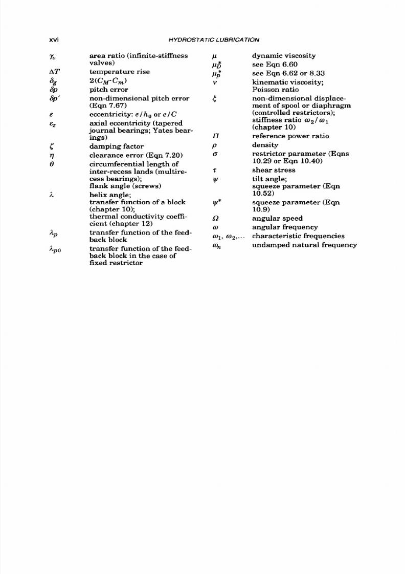
Lis t
of main symbols
An inverted comma
(')
generally indicates tha t the relevant quantity has been
made non-dimensional by dividing it by a suitable reference value (often the value in
the reference configuration, when it is applicable); since the reference values may
depend on the bearing type and on the type of supply system, only a few have been
indicated below.
Meaning of most frequently used subscripts:
generally means 'in the reference configuration', that is, in particular, the
centred o r concentric configuration whenever it is applicable; in chapter 11
generally indicates a suitable (although arbitrary) value used a s reference in
the optimization process;
means 'land';
mean 'maximum' and 'minimum', respectively;
means 'restrictor' or 'recess';
in chapter 10 refers
to
the static equilibrium configuration, except for p s
(supply pressure), whereas in chapter
12
refers t o the land area of a pad;
refers to controlled restrictors.
effective area
nondimensional effective
area
effective friction area
land area
recess area
effective area of spool o r di-
aphragm (controlled restric-
tors)
land length
a l L
or
u l ( r 4 - r l )
characteristic parameter of
flow dividers (Eqn 7.49)
pad width;
squeeze coefficient (pad bear-
ings) or damping coefficient
(journal bearings)
B'
BO
b
b'
C
D
e
F
f
C
Ff
B I L ;
B
I
Bo (single pad and self-
regulating bearings);
BI 2Bo
(opposed-pad b.)
reference squeeze coefficient
of a pad or reference damp-
ing coefficient of a journal
bearing
recess width
b l B
radial clearance
specific heat
diameter
displacement
loading force
friction force
friction coefficient
8/9/2019 Hydrostatic Lubrication 1992
http://slidepdf.com/reader/full/hydrostatic-lubrication-1992 16/558
LIST OF SYMBOLS
xv
recess friction factor
Qpc (chapter
12)
see Eqn 12.7
actual value of axial play
(opposed-pad bearings)
friction power
nondimensional friction
parameter
reference friction power of a
Pad
H f I H f o
single pad and self-
regulating bearings);
H f l 2 H f 0
(opposed-padb.)
land friction power
recess friction power
pumping power (dissipated
in a pad)
pumping power
total power
see Eqn
6.58
o r
8.32
film thickness
normal film thickness
(tapered pads)
recess depth
stiffness
reference stiffness
reference stiffness for capil-
lary compensation
stiffness of lubricant (Eqn
10.19)
equivalent bulk modulus
tilting stiffness
stiffness of spring or di-
aphragm (controlled restric-
tors)
speed enhancement factor
speed parameter (chapter 11)
bearing length
recess length
IIL
moment;
mass
friction moment
number of recesses;
number of active turns
(screw-nut assemblies)
pitch
KIKo
P r
P s
Q
R
R*
R’
RO
R i
Re
Rr
r
r’
6
Sh
Si
T
Ta
Tt?
Ti
U
V
W
wf2
wz
X
a
8
8”
Y
recess pressure
supply pressure
flow rate
hydraulic resistance;
thermal resistance (chapter
12)
nondimensional resistance
parameter
RI R, (pad bearings)
reference hydraulic resis-
tance of a pad
R I R o (self-regulating bear-
ings)
Reynolds number
hydraulic resistance of com-
pensating restrictor
radius
inner
to
outer radius ratio
rllr2
(self-regulating bear-
ings)
velocity parameter (Eqn
8 . 8 )
inert ia parameter
temperature
ambient temperature
temperature
at
the outlet of
a land (chapter
1 2 )
temperature at the inlet of a
land (chapter 12)
sliding speed
volume of recess and rele-
vant supply pipe (chapter 10)
load capacity
hydrodynamic load capacity
axial load capacity (tapered
or spherical journal bear-
ings; Yates bearings)
displacement of spool o r
diaphragm (controlled re-
strictors)
half-cone angle;
thermal conductance
(chapter 12)
reference pressure ratio
valve parameter
load angle (spherical journal
bearings);
reference pressure ratio (self-
regulating bearings)
8/9/2019 Hydrostatic Lubrication 1992
http://slidepdf.com/reader/full/hydrostatic-lubrication-1992 17/558
HYDROSTATIC LUB RICA TlON
area ratio (infinite-stiffness
valves)
temperature rise
pitch error
non-dimensional pitch error
(Eqn
7.67)
eccentricity:e l h o o r e l C
axial eccentricity (tapered
journal bearings; Yates bear-
ings)
damping factor
clearance error (Eqn 7.20)
circumferential length of
inter-recess lands (multire-
cess bearings);
flank angle (screws)
helix angle;
transfer function of a block
(chapter 10);
thermal conductivity coefi-
cient (chapter 12)
transfer function of the feed-
back block
transfer function of the feed-
back block in the case of
fixed restrictor
2(C&f-C,)
dynamic viscosity
see Eqn 6.60
see Eqn
6.62 o r 8.33
kinematic viscosity;
Poisson ratio
non-dimensional displace-
ment of spool or diaphragm
(controlled restrictors);
stiffness ratio
w 2 / w 1
(chapter 10)
reference power ratio
density
restrictor parameter (Eqns
10.29
or
Eqn 10.40)
shear stress
tilt angle;
squeeze parameter (Eqn
10.52)
squeeze parameter (Eqn
10.9)
angular speed
angular frequency
characteristic frequencies
undamped natural frequency

8/9/2019 Hydrostatic Lubrication 1992
http://slidepdf.com/reader/full/hydrostatic-lubrication-1992 18/558
Chapter
1
HYDROSTATIC BEARINGS
1.1 INTRODUCTION
Hydrostatic lubrication consists in pushing a lubricant between the surfaces of
a kinematic pair by means
of
an external pressurization system. This lubrication
mechanism has now a well-defined collocation in the large field of lubrication engi-
neering. In particular, it can be used instead of hydrodynamic lubrication when
this last proves t o be not very effective. The main advantages of externally pressur-
ized lubrication are very low friction and negligible wear, whereas the only actual
drawback is a certain complexity of supply circuits. Applications thus vary from
large, generally slow, machines to small, generally fast, machines: this is also
made possible by the wide range of kinematic pairs to which hydrostatic lubrication
can be applied.
1.2 WORKING PRINCIPLE
It is well known that, to ensure the setting up and the persistence of a steady
hydrodynamic pressure field in the lubricant separating the surfaces of any kine-
matic pair, two important conditions have to be met:
- the mating surfaces must not be parallel;
-
a sufficient relative velocity must exist.
When one,
o r
both, of these conditions cannot be satisfied, an “external pressur-
ization” of the lubricant may be the solution: the pressurized field allows the lift and
the bearing of the moving member on the fixed member of the pair.

8/9/2019 Hydrostatic Lubrication 1992
http://slidepdf.com/reader/full/hydrostatic-lubrication-1992 19/558
2
HYDROSTATIC LUBRICATION
Fig.
1.1
contains an outline of the principle of "externally pressurized lubrica-
tion", which is most commonly referred
t o
as "hydrostatic lubrication". The recess
(of which the projected area is
A)
of the bearing pad [ll
of
the pair is fed by
a
pump;
the bearing runner [21 is loaded by a force
W
(Fig. 1.l.a). When the pump begins
t o
run, the pressure in the recess grows (Fig. l.l.b), until the "lifting pressure"
p = W I A
is reached (Fig. 1.1 .~ ); t this point member
121
is lifted,
a
lubricant film
builds up to separate the surfaces, and a
flow
Q
is delivered, due
t o
the pressure step
along the clearance (Fig. 1.l.d). Different loads lead to different values of the recess
pressure and of the film thickness
h
(Fig. l.l.e, f).
Fig.
1.1 Hydrostatic lubrication: pressure diagrams and
fluid
film formation in
an
axial single-pad
bearing.
To
also sustain loads in the reverse direction, member
[21
is put between two
pads
[l],
s shown in Fig.
1.2. Now
flows
Q
cause recess pressures
p>O
even for
W=O:
the system is preloaded (Fig. 1.2.a.). When a load
W
is applied, the pressure in
8/9/2019 Hydrostatic Lubrication 1992
http://slidepdf.com/reader/full/hydrostatic-lubrication-1992 20/558
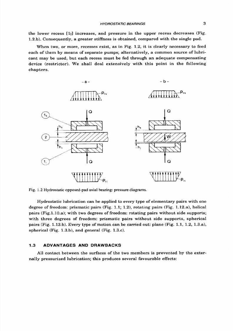
HYDROSTATIC BEARINGS 3
the lower recess [11] increases, and pressure in the upper recess decreases (Fig.
1.2.b). Consequently, a greater stiffness is obtained, compared with th e single pad.
When two, o r more, recesses exist, as in Fig. 1.2, it is clearly necessary
t o
feed
each of them by means of separate pumps; alternatively, a common source of lubri-
cant may be used, but each recess must be fed through an adequate compensating
device (restrictor). We shall deal extensively with th is point in the following
chapters.
- a - - b -
r i t t t l t t trPr,
Fig. 1.2Hydrostatic opposed-pad axial bearing: pressure diagrams.
Hydrostatic lubrication can be applied to every type
of
elementary pairs with one
degree
of
freedom: prismatic pairs (Fig. 1.1; 1.2), rotating pairs (Fig. 1.12.a), helical
pairs (Fig.l.1O.a); with two degrees of freedom: rotating pairs without side supports;
with three degrees of freedom: prismatic pairs without side supports, spherical
pairs (Fig. 1.13.b). Every type of motion can be carried out: plane (Fig. 1.1, 1.2, 1.3.a),
spherical (Fig. 1.3.b), and general (Fig. 1.3.c).
1.3
ADVANTAGES AND DRAWBACKS
All contact between the surfaces of the two members is prevented by the exter-
nally pressurized lubrication; this produces several favourable effects:

8/9/2019 Hydrostatic Lubrication 1992
http://slidepdf.com/reader/full/hydrostatic-lubrication-1992 21/558
4
HYDROSTATIC LUBRICATION
- no wear practically exists;
- friction can be very low, especially when the relative velocity of the surfaces is low;
- no stick-slip exists;
-
stiffness can be considerable: i.e. a very slight variation in the thickness of the lu-
bricant film may be obtained, for any given variation of the load;
- the lubricant film produces an "averaging" of the roughness and the other defects
of the mating surfaces;
-
no localized overpressure exists: the pressure field is uniform in the recesses
(which are generally large) and decreases in the clearances;
- the pressurized fluid film has high damping characteristics;
-
the effectiveness of the lubrication is hardly influenced at all by thermal problems
and by a n y variation in the speed regime;
- every fluid may, in principle, be used as a lubricant;
-
the performance of the hydrostatic bearings is simpler
t o
evaluate than in the case
of hydrodynamic bearings, since the boundary conditions are, generally, well
defined.
The main drawback consists in the need for a supply system, a t medium
o r
high pressure, with the relevant control and safety devices. However, some sort of
supply system is generally required in hydrodynamic lubrication, and even for
rolling bearings.
In Table 1.1 the hydrostatic slideways, journal bearings, and screw-nut assem-
blies are compared with analogous usual pairs, to give some rough direction for the
effective use of externally pressurized lubrication.
1.4 APPLICATIONS
The first application of hydrostatic lubrication was carried out by the French-
man
L.
D. Girard, who, in the second half of the last century, built a water hydro-
static journal bearing (ref.
1.1)
and, subsequently, thrust bearings, too.
In the second decade of this century, a hydrostatic annular thrust bearing was
applied in a hydraulic turbine, see ref. 1.2, and Lord Rayleigh worked out the equa-
tions for calculating load capacity, lubricant flow rate, and friction moment for a
circular thrust bearing (ref.
1.3).
In the third decade an interesting and spectacular application of hydrostatic
lubrication was that of the Hale telescope of Mount Palomar (ref. 1.4).
Several authors, of whom D. D. Fuller (ref. 1.51, H.
C.
Rippel (ref. 1.6), nd H.
Opitz (ref.
1.7)
deserve special mention, subsequently contributed to the development
of hydrostatic bearings.
8/9/2019 Hydrostatic Lubrication 1992
http://slidepdf.com/reader/full/hydrostatic-lubrication-1992 22/558
HYDROSTATIC BEARINGS
5
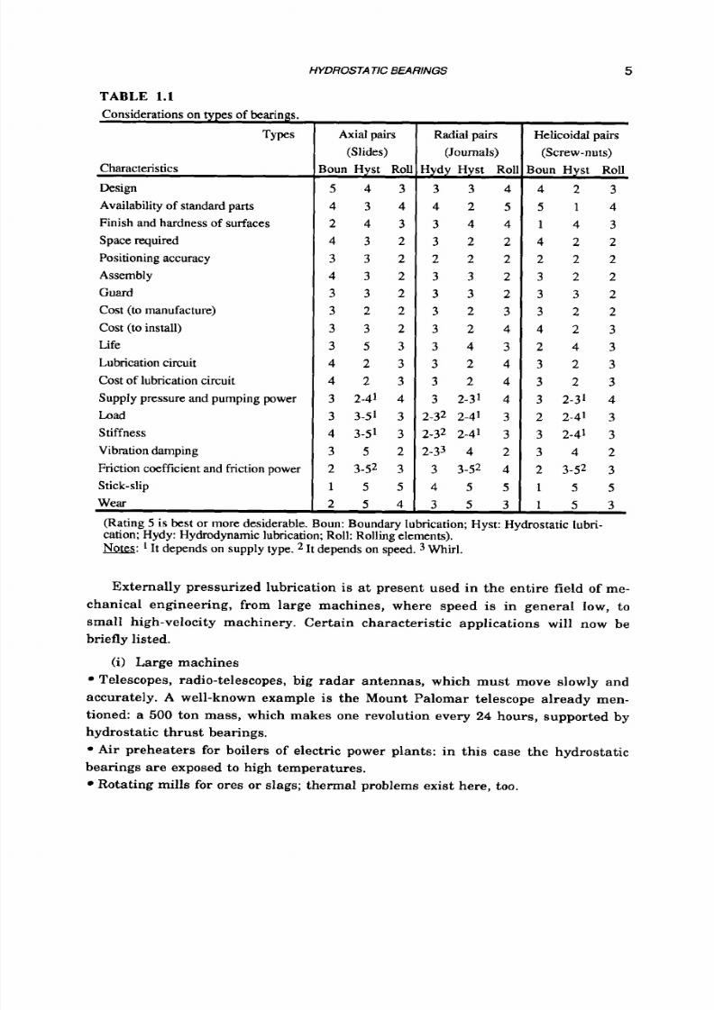
TABLE
1.1
Considerations on types of bearings.
Types
Characteristics
Design
Availability of standard parts
Finish and hardness of surfaces
Space required
Positioning accuracy
Assembly
Guard
Cost (to m anufacture)
Cost (to install)
Life
Lubrication circuit
Cost of lubrication circuit
Supply pressure and pumping power
Load
Stiffness
Vibration damping
Friction coefficient and friction power
Stick-slip
Wear
~~
Axial pairs
(Slides)
Boun Hyst Rol
5 4 3
4 3 4
2 4 3
4 3 2
3 3 2
4 3 2
3 3 2
3 2 2
3 3 2
3 5 3
4 2 3
4 2 3
3 2-41 4
3 3-51
3
4 3-51 3
3 5 2
2 3-52 3
1 5 5
2 5 4
Radial pairs
(Journals)
Hydy Hys t Rol
3 3 4
4 2 5
3 4 4
3 2 2
2 2 2
3 3 2
3 3 2
3 2 3
3 2 4
3 4 3
3 2 4
3 2 4
3 2-31 4
2-32 2-41 3
2-32 2-4' 3
2-33 4 2
3 3-52 4
4 5 5
3 5 3
Helicoidal pairs
(Screw-nuts)
3oun Hys t Roll
4 2 3
5 1 4
1 4 3
4 2 2
2 2 2
3 2 2
3 3 2
3 2 2
4 2 3
2 4 3
3 2 3
3 2 3
3 2-31 4
2 2-41 3
3 2-41 3
3 4 2
2 3-52 3
1 5 5
1 5 3
(Rating
5
is best or more desiderable. Boun: Boundary lubrication; Hyst: Hydrostatic lubri-
cation; Hydy: Hydrodynamic lubrication; Roll:
Rolling
elements).
&@:
It depends on supply type. It depends on speed.
3
Whirl.
Externally pressurized lubrication is at present used in the entire field of me-
chanical engineering, from large machines, where speed
is
in general low,
t o
small high-velocity machinery. Certain characteristic applications will now be
briefly listed.
(i) Large machines
Telescopes, radio-telescopes, big radar antennas, which must move slowly and
accurately.
A
well-known example is the Mount Palomar telescope already men-
tioned: a 500 ton mass, which makes one revolution every 24 hours, supported by
hydrostatic thrust bearings.
Air preheaters for boilers
of
electric power plants:
in
this case the hydrostatic
bearings are exposed to high temperatures.
Rotating mills for ores
o r
slags; thermal problems exist here, too.
8/9/2019 Hydrostatic Lubrication 1992
http://slidepdf.com/reader/full/hydrostatic-lubrication-1992 23/558
6
HYDROSTA TIC LUBRICA
TlON
Machine tools (ref. 1.8),where medium or high precision is required t o move
great weights; for instance large boring or milling machines. The moving car-
riages are supported by hydrostatic slideways and are sometimes driven by hydro-
static screw and nut assemblies.
Hydrostatic steady rests for large lathes.
Assembly lines, where the component parts are carried along on hydrostatic
slides; this allows a very accurate positioning of the components.
Structures, even of very large ones, which can be easily moved on hydrostatic
bearings.
(ii) Medium size machines
Grinding machines, numerical control machine tools, machining centers, which
require very accurate positioning and freedom from vibration. Due to the absence of
stick-slips, and
t o
the high degree of stiffness and damping of the pressurized fluid
film, hydrostatic lubrication is particularly suitable for such machines.
High velocity spindles; in this application hydrostatic bearings often prove to be
better than hydrodynamic ones (particularly in the start and stop stages) as well as
being better than the rolling bearings (where some problems are encountered, due
to the effects of wear and
t o
the high centrifugal forces on the rollers).
(iii) Small machines
Precision balances, dynamometers: hydrostatic bearings are better than the usual
ones, because friction practically vanishes at very low speeds, even in the case of
alternate motion. Their use is particularly advisable for electrical rotating-field
dynamometers.
Vibration attenuators for measuring instruments.
Frictionless oil seals; these seals may be useful in certain cases e.g.: distributors
of lubricant f o r hydrostatic slideways, hydraulic cylinders for flight simulators.
- a -
- b -
. _
I
- c -
i-
t-----+--
w
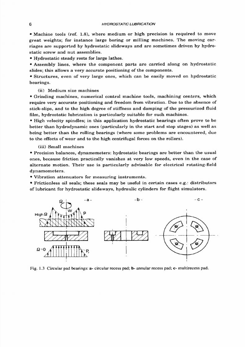
Fig. 1.3 Circular
pad
bearings:
a-
circular recess
pad; b-
annular recess
pad; c-
multirecess
pad.

8/9/2019 Hydrostatic Lubrication 1992
http://slidepdf.com/reader/full/hydrostatic-lubrication-1992 24/558
HYDROSTATIC
BEARINGS
7
1.5 TYPES
OF BEARINGS
Hydrostatic bearings may be classified on the basis of the direction
of
the load
that may be carried.
S o
we have:
- thrust bearings;
- radial bearings (journal bearings);
- multidirectional bearings.
Let us examine briefly the most common shapes.
1.5.1 Thrust bearings
(i) Circu lar p a d bearings . Figure 1.3 shows: -a- a central-recess pad; -b- an
annular recess pad; -c- a multirecess pad.
A s
rotary speed becomes very high, the
behavior of pad -a- becomes "hybrid": hydrodynamic pressure, caused by centrifu-
gal force, joins the hydrostatic pressure (see section 6.3.l(vi)). Provided each recess
is independently fed, pad -c- may also sustain tilting moments.
(ii) Opposed-pad circular bearings. When the load may act in two opposite di-
rections, o r when greater stiffness is needed, two circular pads may be assembled
as shown in Fig. 1.4.a. If the load has a prevalent direction, it may be found useful
to select two different pads (Fig. 1.4.b).
The bearing in Fig. 1.4.c is a "self-regulating" one; i.e., thanks
t o
its shape, the
flow rates supplied to the two halves of the bearing are always equal to each other.
Consequently, only one supply device is needed.
(iii) Rectangular pad bear ings .
A
number of shapes of rectangular pads are
- a -
- b -
- c -
Fig. 1.4 Opposed-pad circular bearings: a- equal pads; b - unequal pads; c- "self-regulating"
bearing.
8/9/2019 Hydrostatic Lubrication 1992
http://slidepdf.com/reader/full/hydrostatic-lubrication-1992 25/558
8 HYDROSTATIC LUBRICATION
+-
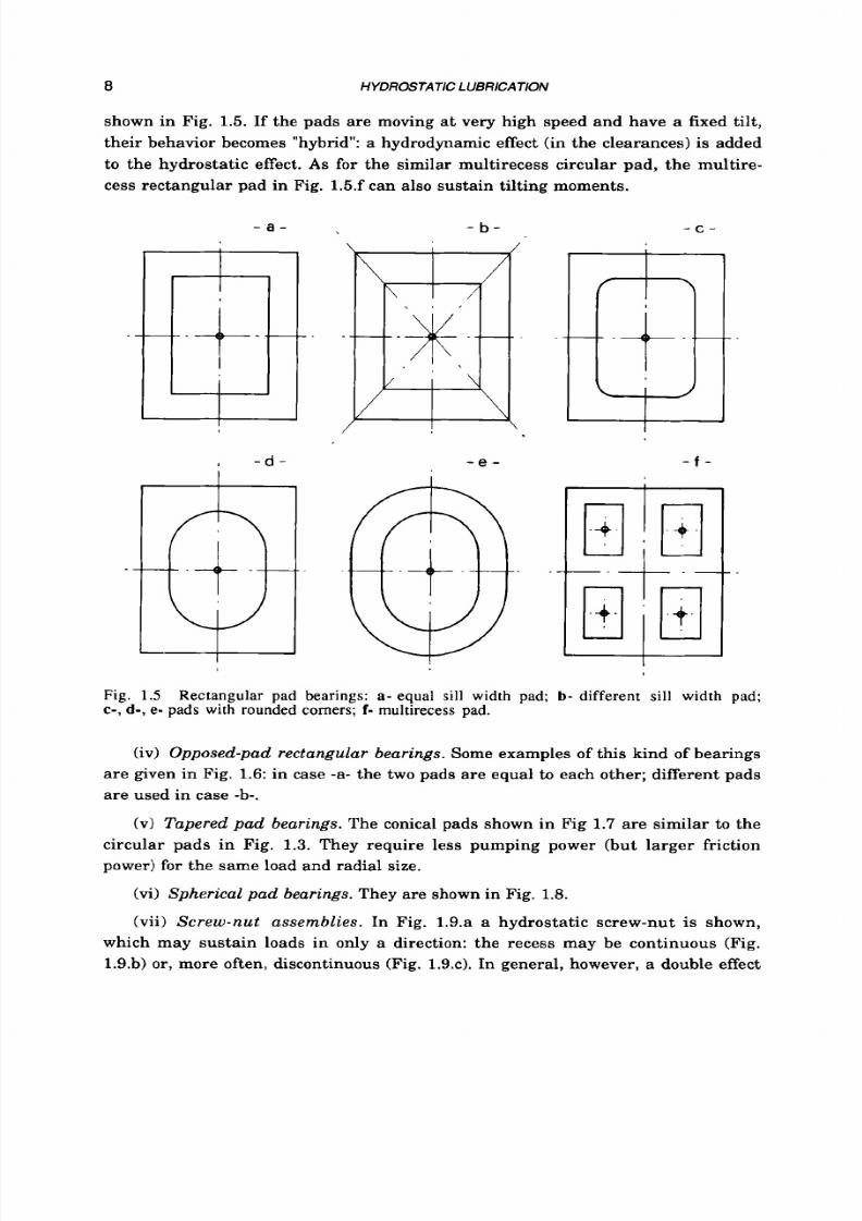
shown in Fig. 1.5. If the pads are moving at very high speed and have a fixed tilt,
their behavior becomes "hybrid": a hydrodynamic effect (in the clearances) is added
to the hydrostatic effect. As for the similar multirecess circular pad, the multire-
cess rectangular pad in Fig. 1.5.f can also sustain tilting moments.
- a -
I - d -
I
-
b -
- e -
- c -
- f -
Fig.
1.5
c-, d- , e- pads with rounded comers; f- rnultirecess pad.
Rectangular pad bearings:
a -
equal
sill
width pad; b - different sill width pad;
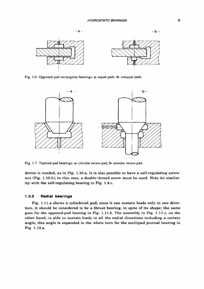
(iv) Opp osed-pa d rectangular bearings. Some examples of this kind of bearings
are given in Fig.
1.6:
in case -a- the two pads are equal to each other; different pads
are used in case -b-.
(v)
Tapered pa d bearings.
The conical pads shown in Fig 1.7 are similar
t o
the
circular pads in Fig. 1.3. They require less pumping power (but larger friction
power) for the same load and radial size.
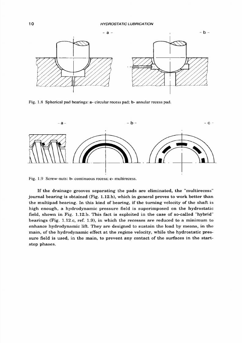
(vi) Spherical pa d bearings. They are shown in Fig. 1.8.
(vii) Screw-nut as sembl ie s . In Fig. 1.9.a a hydrostatic screw-nut is shown,
which may sustain loads in only a direction: the recess may be continuous (Fig.
1.9.b) or, more often, discontinuous (Fig. 1.9.~) .n general, however, a double effect
8/9/2019 Hydrostatic Lubrication 1992
http://slidepdf.com/reader/full/hydrostatic-lubrication-1992 26/558
HYDROSTATIC BEARINGS
9
- a - - b -
Fig. 1.6
Opposed-pad rectangular
bearings:
a- equal pads; b- unequal pads.
- a -
'
- b -
I
Fig.
1.7
Tapered pad bearings: a- circular recess pad; b- annular recess pad.
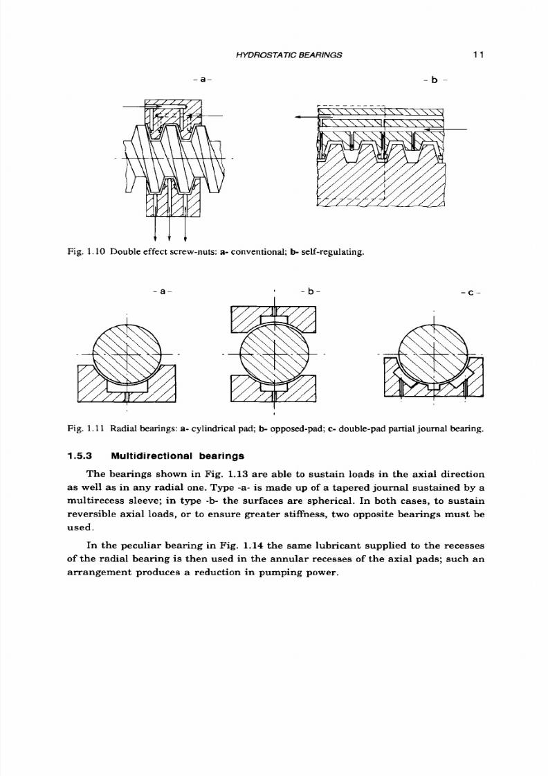
device
is
needed, as in Fig. l.lO.a. It is also possible to have a self-regulating screw-
nut (Fig. 1.lO.b); in this case, a double-thread screw must be used. Note
its
similar-
ity with the self-regulating bearing in Fig. 1.4.c.
1.5.2
Radial
bear ings
Fig. 1 .ll .a shows a cylindrical pad; since it can sustain loads only in one direc-
tion, it should be considered to be a thrust bearing, in spite of its shape; the same
goes for the opposed-pad bearing in Fig. l.ll.b. The assembly in Fig. l.ll.c, on the
other hand, is able t o sustain loads in all the radial directions including a certain
angle; this angle is expanded to the whole turn for the multipad journal bearing in
Fig. 1.12.a.
8/9/2019 Hydrostatic Lubrication 1992
http://slidepdf.com/reader/full/hydrostatic-lubrication-1992 27/558
10 HYDROSTATIC LUBRICATION
- a -
- b -
Fig.
1.8
Spherical pad bearings:
a-
circular recess pad
b-
annular recess
pad.
- a - - b -
. _
- c
Fig. 1.9
Screw-nuts:
b-
continuous recess; c- multirecess.
If the drainage grooves separating the pads are eliminated, the "multirecess"
journal bearing is obtained (Fig. 1.12.b), which in general proves to work bette r than
the multipad bearing. In this kind of bearing, if the turning velocity of the shaft is
high enough, a hydrodynamic pressure field is superimposed on the hydrostatic
field, shown in Fig. 1.12.b. This fact is exploited in the case of so-called "hybrid"
bearings (Fig. 1.12.c, ref. 1.9), in which the recesses a re reduced to a minimum
t o
enhance hydrodynamic lift. They are designed
t o
sustain the load by means, in the
main, of the hydrodynamic effect a t the regime velocity, while the hydrostatic pres-
sure field
is
used, in the main, to prevent any contact
of
the surfaces i n the start-
stop phases.
8/9/2019 Hydrostatic Lubrication 1992
http://slidepdf.com/reader/full/hydrostatic-lubrication-1992 28/558
HYDROSTATIC BEARINGS
- a -
- b -
11
t t 1
Fig.
1.10
Double effect screw-nuts:
a-
conventional;
b-
self-regulating.
- a -
-
b -
- c -
Fig.
1.11
Radial bearings:
a-
cylindrical pad;
b-
opposed-pad;
c-
double-pad partial journal bearing.
1.5.3 Mult id i rect ional bear ings
The bearings shown in Fig. 1.13 are able to sustain loads in the axial direction
as well as in any radial one. Type -a- is made up of a tapered journal sustained by a
multirecess sleeve; in type -b- the surfaces are spherical. In both cases, t o sustain
reversible axial loads, o r to ensure greater stiffness, two opposite bearings must be
used.
In the peculiar bearing in Fig.
1.14
the same lubricant supplied t o the recesses
of the radial bearing is then used in the annular recesses of the axial pads; such an
arrangement produces a reduction in pumping power.

8/9/2019 Hydrostatic Lubrication 1992
http://slidepdf.com/reader/full/hydrostatic-lubrication-1992 29/558
12
HYDROSTATIC LUBRICATION
c
-
- a -
I
Fig. 1.12Journal bearings:a- multipad; b- multirecess;
c-
hybrid.
- a -
i
- c -
I
I
Fig. 1.13 Multidirectionalbearings:
a-
conical bearing; b- spherical bearing.
Fig.
1.14
"Yates"bearing.

8/9/2019 Hydrostatic Lubrication 1992
http://slidepdf.com/reader/full/hydrostatic-lubrication-1992 30/558
HYDROSTATIC
BEARINGS
13
1.5.4 Bear ing arrangements
Hydrostatic bearings are variously combined to build hydrostatic bearing
systems.
Figure 1.15.a shows a spindle which is sustained by a journal bearing on the
right-hand side, and by
a
combined axial and radial bearing
on
the other side;
whereas, in Fig. 1.15.b, the spindle is sustained by a pair of conical bearings.
- a -
- b -
Fig.
1.15
Hyd rostatic spindle: a- with a journal bearing and a com bined journal and thrust bearing;
b-
with two conical bearings.
Fig. 1.16 Hydro static slideway.
8/9/2019 Hydrostatic Lubrication 1992
http://slidepdf.com/reader/full/hydrostatic-lubrication-1992 31/558
14
HYDROSTATIC
LUBRICATION
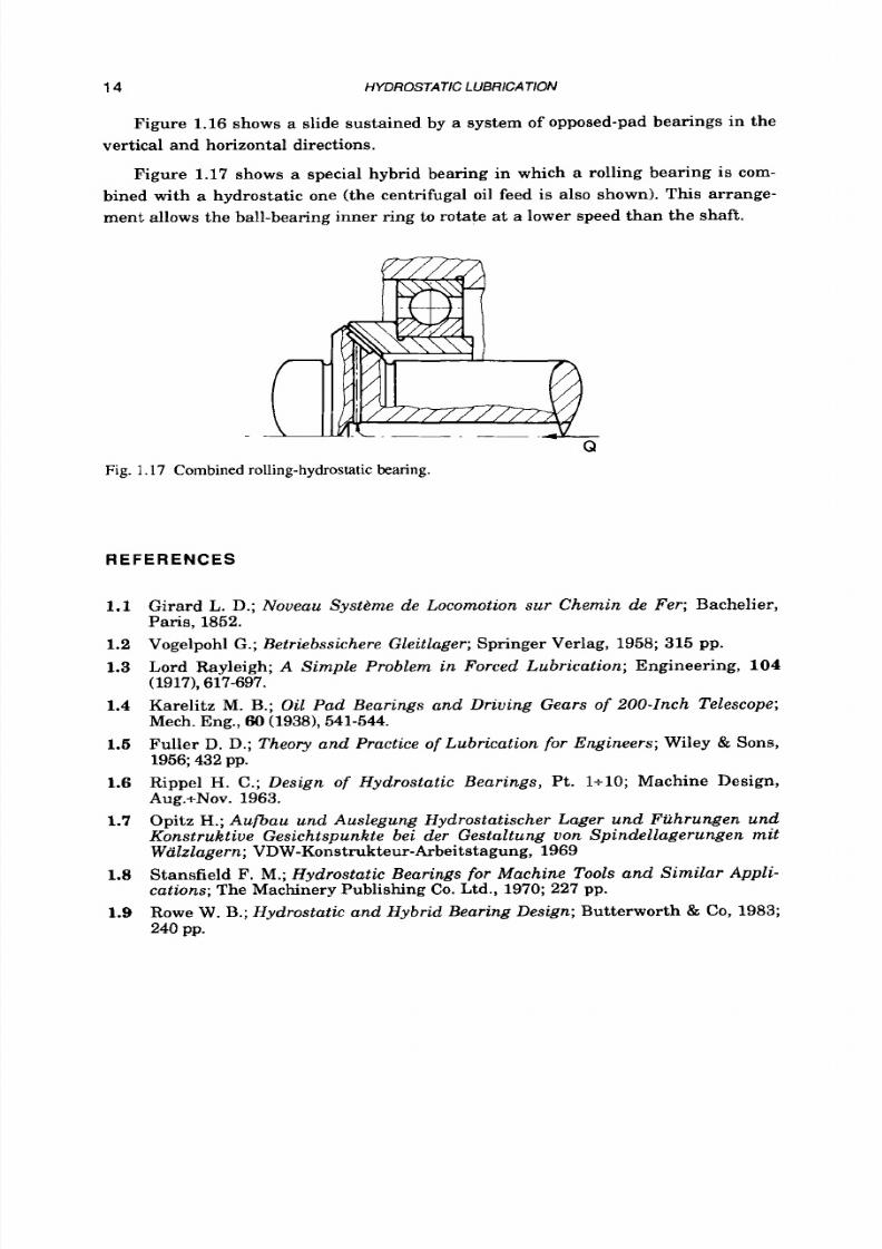
Figure 1.16 shows a slide sustained by a system of opposed-pad bearings in the
vertical and horizontal directions.
Figure
1.17
shows a special hybrid bearing in which
a
rolling bearing is com-
bined with a hydrostatic one (the centrifugal oil feed is also shown). This arrange-
ment allows the ball-bearing inner ring
to
rotate a t a lower speed than the shaft.
Fig.
1.17 Combined rolling-hydrostatic
bearing.
R E F E R E N C E S
1.1
1.2
1.3
1.4
1.5
1.6
1.7
1.8
1.9
Girard
L.
D.;
Noueau S ystkme de Locomotion
sur
Ch e m in d e F e r;
Bachelier,
Paris, 1852.
Vogelpohl G.;
Betriebssichere Gleitlager;
Springer Verlag,
1958; 315
pp.
Lord Rayleigh; A
Simple Problem
in
Forced Lubrication;
Engineering, 104
Karelitz M. B.;
Oil Pad Bearings and Driving Gears of 200-Znch Telescope;
Mech. Eng., 60 19381,541-544.
Fuller
D.
D.;
Theory and Practice
of
Lubrication
for
Engineers;
Wiley
&
Sons,
1956; 432 pp.
Rippel H. C.;
Design
of
Hydros tat ic Bear ings ,
Pt. lt10; Machine Design,
Aug.+Nov.
1963.
Opitz
H.; Aufbau und Auslegung Hydros tat ischer Lager und Fu hrungen und
Konstruktive Gesichtspunkte bei der Gestaltung von Spindellagerungen
mit
Walzlagern;
VDW-Konstrukteur-Arbeitstagung, 1969
Stansfield F. M.;
Hydrostatic Bearings
for
Machine Tools and Sim ilar Appl i -
cations; The Machinery Publishing Co. Ltd., 1970; 227 pp.
Rowe
W. B.; Hydrostatic and Hybrid Bearing Design;
Butterworth
&
Co,
1983;
240
pp.
(1917),617-697.
8/9/2019 Hydrostatic Lubrication 1992
http://slidepdf.com/reader/full/hydrostatic-lubrication-1992 32/558
Chapter 2
COMPENSATING DEVICES
2.1
INTRODUCTION
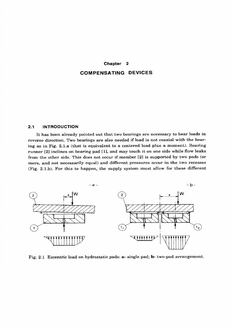
It has been already pointed out that two bearings a re necessary to bear loads in
reverse direction. Two bearings are also needed if load
is
not coaxial with the bear-
ing
as
i n Fig. 2.1.a (t hat
is
equivalent to a centered load
plus a
moment). Bearing
runner [2] inclines on bearing pad [l], and may touch it on one side while flow leaks
from the other side, This does not occur if member [2] is supported by two pads (or
more, and not necessarily equal) and different pressures occur in the two recesses
(Fig. 2.1.b). For this t o happen, the supply system must allow for these different
- a - - b -
tt'tttlLv
Fig. 2.1 Eccentric load on hydrostatic pads:
a-
ingle pad;
b-
wo-pad arrangement.
8/9/2019 Hydrostatic Lubrication 1992
http://slidepdf.com/reader/full/hydrostatic-lubrication-1992 33/558
16
HYDROSTATIC LUBRlCATlON
pressures. In practice this may be accomplished in two ways:
- by using a separate pump t o feed each recess directly; this is commonly referred t o
as the "constant-flow supply system";
-
by using a common source of pressurized lubricant, which is carried
t o
each pad
through compensating devices (restrictors); since the pressure is generally held
constant upstream from the restrictors, this is commonly referred to as the
"constant pressure supply systems".
Furthermore, certain particular types of bearings are proposed that are
"inherently compensated"; i.e. they have a built-in compensating device. In this
way, they can be fed directly by a lubricant source (in general, a t constant pressure).
From the foregoing considerations it is clear that the proper working of the
hydrostatic bearings depends on the correct selection of the devices which make up
the supply system, as well as on the correct design of the bearing itself.
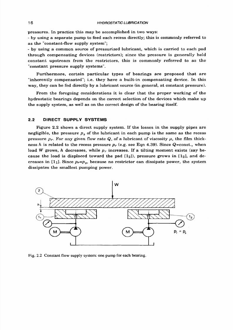
2.2 DIRECT
SUPPLY
SYSTEMS
Figure 2.2 shows a direct supply system. If the losses in the supply pipes are
negligible, the pressure
ps
of the lubricant in each pump is the same as the recess
pressure
Pr.
For any given flow rate Q,
of a
lubricant of viscosity
p,
he film thick-
ness
h
is related t o the recess pressure
Pr
(e.g. see Eqn 4.39).Since &=const., when
load W grows, h decreases, while Pr increases. If a tilting moment exists (say be-
cause the load is displaced toward the pad [12]), pressure grows in [12], and de-
creases in [11]. Since Pr=Ps, ecause no restrictor can dissipate power, the system
dissipates the smallest pumping power.
h
Fig.
2.2 Constant
flow
supply system: on e pump
for
each
bearing.

8/9/2019 Hydrostatic Lubrication 1992
http://slidepdf.com/reader/full/hydrostatic-lubrication-1992 34/558
COMPENSATING DEVICES 17
In theory, the only limitation to the increase ofp,, and hence of the load capacity
(and stiffness) of the bearing, comes from the power of the motor, and from the
maximum allowable pressure in the supply system.
In the last analysis, the constant flow system proves to be quite efficient. Its
limit
is
of an economic nature, due to the need for a pump, with the relevant motor,
for each recess. The problem can be partially overcome, particularly when all the
pumps are equal, all being driven by means of a single motor. It is worth noting
that this method also makes it possible to reduce the power required, lower than the
sum of the peak power required for each pump.
Figure
2.3
shows a particular arrangement (ref.
2.1),
in which a motor drives
a
main pump (which steps up pressure to an intermediate value) and at the same
time
a
series of smaller pumps feeding the recesses. The delivery of the main pump
is a little greater than the sum of the flow rate of the other pumps. Such an ar-
rangement makes it possible t o reduce the pressure step in the pumps, and th e re-
lated problems, especially in the case of gear pumps.
j
y d r o s ta t i c B e a r i n g s
- - - - .
- -
- . - -
Fig.
2.3
Constant f l o w
supply system: double pressure step.
Another arrangement
is
shown in Fig.
2.4
(ref.
2.2).
The main pump supplies
the two (or more) bearings thorough a "flow divider" made up of the same number
of equal gear pumps, connected by a shaft.
A n
eccentric load
W
tends to decrease
the film thickness hz
of
bearing
1121
and to increase the film thickness of bearing
[111;
so the flow rate of gear
[32],
if disconnected, should tend to decrease, while the
flow rate of gear [31] should tend to increase. The connection, forcing them to rotate
at the same speed, make them produce the same flow rate.
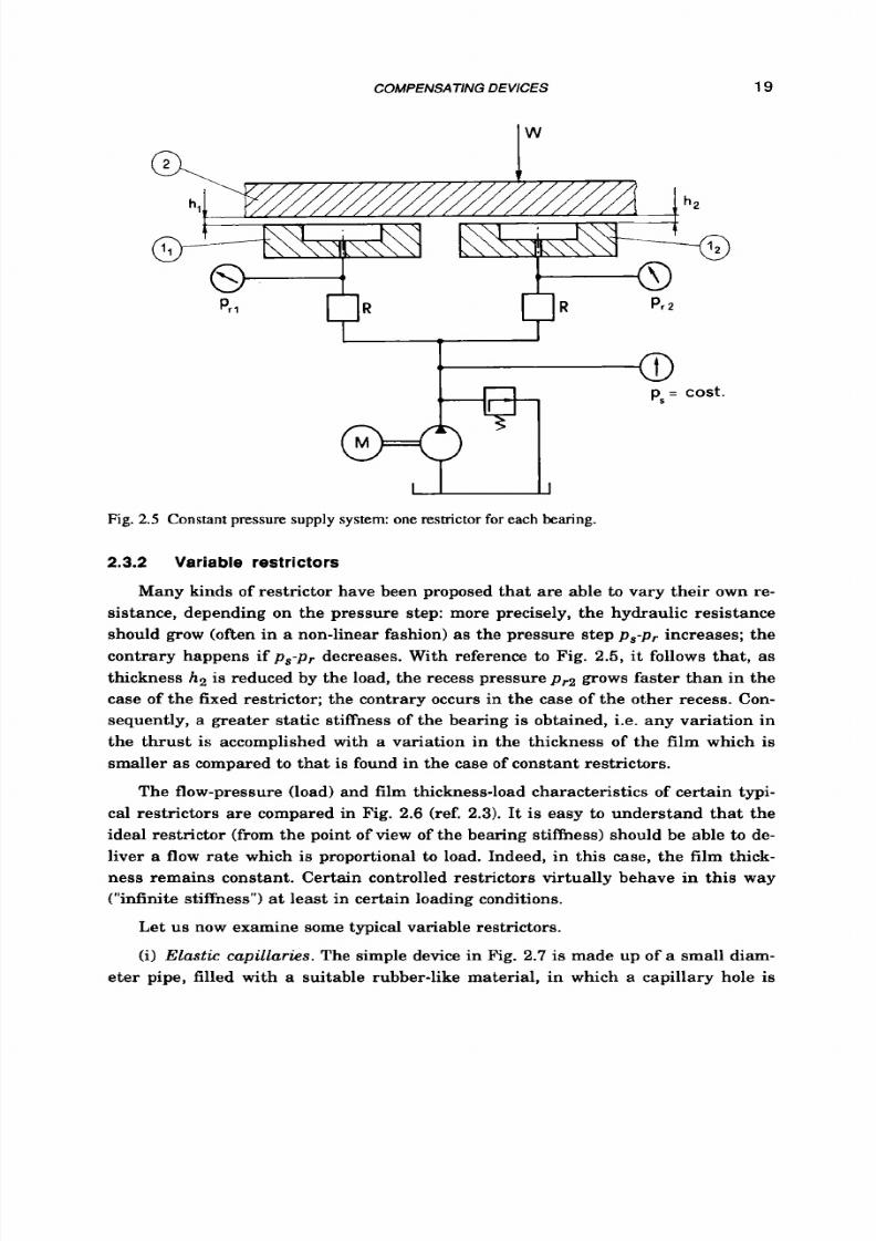
2.3
COMPENSATED SUPPLY SYSTEM
The general layout of a compensated supply system is shown in Fig.
2.5.
The
lubricant delivered by the pump is sent to the recesses of the bearings through the

8/9/2019 Hydrostatic Lubrication 1992
http://slidepdf.com/reader/full/hydrostatic-lubrication-1992 35/558
18
HYDROSTATIC LUBRlCATlON
u
Fig.
2.4 Constant flow supply system: flow
divider.
compensating devices (restrictors)
R i .
The pressure
p s
upstream from the restric-
tors is kept constant by means of
a
suitable regulating system (pressure reducing
valve).
Of
course, the pressure in every recess is always less than
p s
as a conse-
quence of the losses in the restrictors. Many types
of
device can be used, with a fixed
or defonnable geometry.
In the following sections we shall see how the compensating devices work.
2.3.1 Fixed restr ictors
Let
us
assume that the compensating devices in Fig. 2.5 are fixed laminar-flow
restrictors (e.g. capillary tubes). When an eccentric load is applied, the clearance
h2
of the pad
[12]
s squeezed, and so its hydraulic resistance increases. Hence, the
total resistance
of
the series constituted by the restrictor
R2
and the relevant clear-
ance
h 2
also increases. Since pressure
p s
is held constant, the rate
of
flow must de-
crease, so the pressure step
p s - p r 2
must decrease as the rate of flow, until
pr2
reaches a value that balances the load. The contrary happens in the case
of
the
lesser loaded pad
[111.
Orifices can also be used as compensating devices. Unlike the laminar restric-
tors, their hydraulic resistance is no longer a constant. This leads to a slightly bet-
ter performance of the bearing. This point will be dealt with further elsewhere
(chapter
6).
8/9/2019 Hydrostatic Lubrication 1992
http://slidepdf.com/reader/full/hydrostatic-lubrication-1992 36/558
COMPENSATING DEVICES
19
Fig.
2.5 Constant
pressure supply system:
one
restrictor for each
bearing.
2.3.2
Variable rest r ic tors
Many kinds of restrictor have been proposed that are able to vary their own re-
sistance, depending on the pressure step: more precisely, the hydraulic resistance
should grow (often in a non-linear fashion) as the pressure step
p s - p r
increases; the
contrary happens if p s - p P r ecreases. With reference t o Fig. 2.5,
it
follows that, as
thickness
h ,
is reduced by the load, the recess pressure p r 2 grows faster than in the
case of the fixed restrictor; the contrary occurs in the case of the other recess. Con-
sequently, a greater static stiffness of the bearing is obtained, i.e. any variation in
the thrust
is
accomplished with a variation in the thickness of the film which is
smaller
as
compared
t o
that is found in the case of constant restrictors.
The flow-pressure (load) and film thickness-load characteristics of certain typi-
cal restrictors are compared in Fig. 2.6 (ref.
2.3).
It
is
easy to understand that the
ideal restrictor (from the point of view of the bearing stiffness) should be able to de-
liver a
flow
rate which
is
proportional t o load. Indeed, in this case, the film thick-
ness remains constant. Certain controlled restrictors virtually behave in this way
("infinite stiffness") at least in certain loading conditions.
Let us now examine some typical variable restrictors.
(i)
Elast ic capi l laries .
The simple device in Fig.
2.7
is made up of
a
small diam-
eter pipe, filled with a suitable rubber-like material, in which a capillary hole is

8/9/2019 Hydrostatic Lubrication 1992
http://slidepdf.com/reader/full/hydrostatic-lubrication-1992 37/558
20
HYDROSTATIC LUBRICATION
- a -
- b -
Q
h
w
w
Fig.
2.6
Flow rate (a) and
film thickness
(b) versus load for different supply systems:
1-
constant
flow system;
2-
capillary;
3- orifice; 4-
constant
flow
valve; 5- diaphragm-controlled restrictor;
6- infinite stiffness (h=const.).
Fig. 2.7 Plastic throttle.
drilled (ref. 2.4). With any increase in recess pressure p r the hole clearly expands
further, and the hydraulic resistance decreases. Elastic orifices have also been
proposed.
(ii)
Spool-controlled restrictors.
An outline of a
cylindrical-spool valve
is given
in Fig. 2.8.a. The lubricant flows into the small clearance surrounding the spool
[s],
which keeps it s balance due
to
the opposite thrusts exerted by the spring and recess
pressure p r on area
A,.
A s
P r
varies, the length
x
of the restrictor varies
too,
and
so
does it s hydraulic resistance. The shape of the valve may also be th at seen in Fig.
2.8.b.
The tapered-spool valve in Fig.
2.9
works in a similar way (note that the aper-
ture angle is very small). However, since its hydraulic resistance varies faster with
x as compared to the preceding device, it s performance is better (ref. 2.5).
(iii) Diaphragm-controlled restrictors (DCR). In the device shown in Fig. 2.10,
the lubricant
is
drawn through the annular clearance between the inlet duct and
the elastic diaphragm [ml. The device may be tuned by means of the adjustable
spring [s] in such a way that the flow rate becomes almost proportional
t o
p r , thus

8/9/2019 Hydrostatic Lubrication 1992
http://slidepdf.com/reader/full/hydrostatic-lubrication-1992 38/558
COMPENSATlNG DEVICES
- a -
21
- b -
t
PS
Fig. 2.8 Cylindrical-spoolvalves.
I
s
I
ps
pr
\
Fig.
2.9
Tapered-spool valve.
t pr
Fig. 2.10 Diaphragm-controlledvalve.
approaching the infinite stiffness behavior for a certain range of loading condi-
tions (ref. 2.6).
(iv)
Constant-flow
valves. Many kinds of devices able
to
produce a constant flow
rate are widely used in oleodynamic plants. The spool valve in Fig. 2.8 may also be
8/9/2019 Hydrostatic Lubrication 1992
http://slidepdf.com/reader/full/hydrostatic-lubrication-1992 39/558
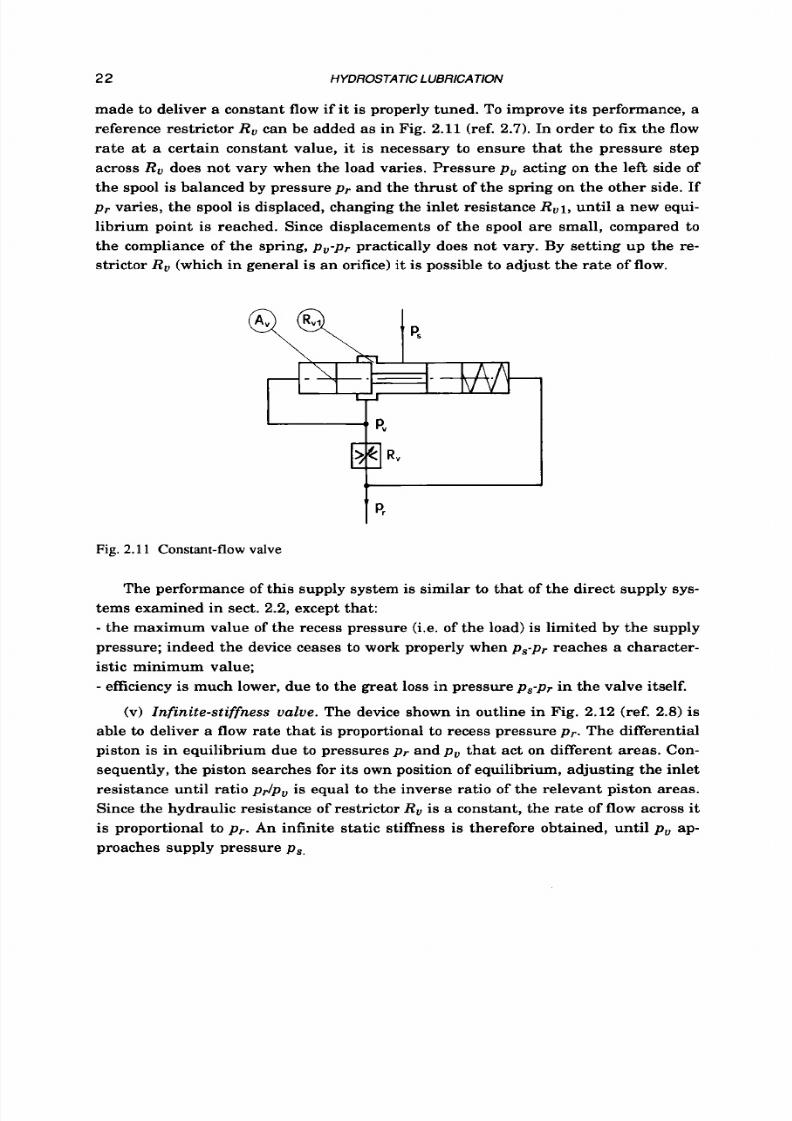
2 2 HYDROSTATIC LUBRICATION
made to deliver a constant flow if it is properly tuned. To improve its performance, a
reference restrictor
RU
an be added as in Fig. 2.11 (ref. 2.7). In order to fix the flow
rate at a certain constant value, it is necessary t o ensure that the pressure step
across
RU
oes not vary when the load varies. Pressure
p , ,
acting on the left side of
the spool is balanced by pressure Pr and the thrust of the spring on the other side. If
p r varies, the spool is displaced, changing the inlet resistance RU1,ntil a new equi-
librium point is reached. Since displacements of the spool are small, compared to
the compliance of the spring, Pu-Pr practically does not vary. By setting up the re-
strictor Ru which in general is an orifice) it is possible to adjust the rate of flow.
Fig. 2.1 1 Constant-flow valve
The performance of this supply system is similar to that of the direct supply sys-
tems examined in sect.
2.2,
except that:
- the maximum value of the recess pressure (i.e. of the load) is limited by the supply
pressure; indeed the device ceases t o work properly when Ps-Pr reaches a character-
istic minimum value;
-
efficiency is much lower, due to the great loss in pressure Ps-pr in the valve itself.
(v) Infinite-stiffness alue.The device shown in outline in Fig.
2.12
(ref.
2.8)
is
able to deliver a flow rate that is proportional to recess pressure P r . The differential
piston is in equilibrium due to pressures P r and p , , that act on different areas. Con-
sequently, the piston searches for it s own position of equilibrium, adjusting the inlet
resistance until ratio pJp , , is equal to the inverse ratio of the relevant piston areas.
Since the hydraulic resistance of restrictor RU s a constant, the rate of flow across it
is proportional to p r . An infinite static stiffness is therefore obtained, until p , , ap-
proaches supply pressure p s .

8/9/2019 Hydrostatic Lubrication 1992
http://slidepdf.com/reader/full/hydrostatic-lubrication-1992 40/558
COMPENSATING DEVICES
23
t
ps
Fig. 2.12 Infinite stiffness valve.
(vi)
Electronic compensators.
All the controlled restrictors cited above are
driven by the recess pressure; new types of variable restrictors have been recently
proposed (ref. 2.24) which are controlled by means of an electromagnetic actuator.
A
feedback signal, drawn by a displacement probe which measures the film thickness
of the bearing (or else by a load cell sensing the force which loads the bearing), is
elaborated by a combination
of
proportional, integral and differential operators and
then amplified in order to drive the actuator.
The benefits of electronic control, confirmed by experimental evidence, consist
in infinite static stiffness, very large dynamic stiffness and short settling time.
moreover the system is not affected by fluctuations
of
supply pressure
o r
lubricant
temperature.
(vii) Flow dividers. When t w o opposite pads have to be fed, as in Fig. 1.12.a, a
flow divider may prove t o be more effective than the use of a separate controlled re-
strictor for each recess.
Most flow dividers are really based on the foregoing controlled restrictors. As an
example, consider the device in Fig. 2.13. When the pressure in any of the two re-
cesses increases, the spool is clearly displaced; hence the lengths of the restrictors
vary, thereby increasing bearing stiffness (ref. 2.9).
The behavior of the tapered-spool flow divider (Fig. 2.14)
is
similar, but its per-
formance is better (ref. 2.10).
Figure 2.15 shows the lay-out of a diaphragm flow divider (ref. 2.11). The restric-
tors are made up of the annular clearances between the diaphragm and the outlet
ducts. If the stiffness of the elastic diaphragm
is
properly selected, a very high
degree of bearing stifiess can be obtained.

8/9/2019 Hydrostatic Lubrication 1992
http://slidepdf.com/reader/full/hydrostatic-lubrication-1992 41/558
24
HYDROSTATIC LUBRICATION
pi
Fig. 2.13 Cylindrical-spoolflow divider.
I
r
I
I
I 1 I
Fig. 2.14 Tapered-spoolflow divider.
Fig.
2.15
Diaphragm-controlled low divider.
Infinite stiffness dividers may also be proposed
(Fig.
2.16),
which are clearly
based on the valve in Fig. 2.12.

8/9/2019 Hydrostatic Lubrication 1992
http://slidepdf.com/reader/full/hydrostatic-lubrication-1992 42/558
COMPENSATING DEVICES
25
Fig. 2.16 Infinite-stiffness
flow
divider.
2.3.3 Inherent ly compensated bearings
The inherently compensated bearingsmain drawback of constant pressure
supply systems is that a considerable fraction of the available pressure step is
dissipated in the external compensating restrictors. To overcome
this
disadvantage
certain inherently compensated bearings have been proposed, all of which are based
on the same principle: the shape of the pressure profile in the bearing clearance is
subject to change with load, due
t o
the peculiar recess shape (Fig. 2.171, o r to the
presence
of
an elastic element, such as a layer of elastomer or a flexible metallic
plate (Fig. 2.18).
Let us take
a
closer look, for instance, a t how the bearing in Fig. 2.17.a (ref. 2.12)
works .
Its distinguishing feature is to have a recess depth
h ,
th at is comparable
with clearance h; consequently, the pressure drop in the recess is no longer negligi-
ble and the shape of pressure profile is that represented by a dashed line. If a higher
load is applied, h is reduced and the ratio
hlh,
increases; it is clear that the pres-
sure drop now tends to concentrate in the clearance, and the pressure profile begins
to take on the typical shape of deep-recess pads, characterized by a constant recess
pressure, making it possible to sustain a higher load without increasing recess
pressure.
Similar considerations could be made in the case of the tapered-recess bearing
in Fig. 2.17.b (ref. 2.13):obviously, in this case, too, the recess depth must be compa-
rable with clearance.
These types of bearings create considerable manufacturing problems (precision
machining of a very shallow recess);
t o
overcome these, the bearing depicted in Fig.

8/9/2019 Hydrostatic Lubrication 1992
http://slidepdf.com/reader/full/hydrostatic-lubrication-1992 43/558
2 6 HYDROSTATIC LUBRICATION
\, ,
,
,
/ / , -
2.18.a (ref. 2.14) has a flat layer of elastomer [ l] bonded to a rigid base. Since pres-
sure decreases from the center to the pad boundary, deformation obviously causes
the development of a "recess" (similar t o the one in Fig. 2.17.b) whose shape varies
with
load.
The flexible-plate bearing in
Fig.
2.18.b (ref. 2.15)works
on
the same principle;
since it is all-metallic, i t is free from problems like rubber-oil compatibility.
, I
\
I,\, ,, A
/ / / / I
- b -
- a -
Fig.
2.17
Inherently compensated bearings:
a-
shallow recess bearing;
b-
tapered-recess bearing.
- a -
-b
-
m
Fig.
2.1
8
Inherently compensated bearings:
a-
elastomeric bearing;
b-
flexible-plate bearing.

8/9/2019 Hydrostatic Lubrication 1992
http://slidepdf.com/reader/full/hydrostatic-lubrication-1992 44/558
COMPENSATING DEVICES 27
Certain bearings have been proposed which have a built-in controlled restrictor.
Let us consider the bearing in Fig. 2.19 (ref. 2.16). I t is supplied at a constant pres-
sure p s . Before entering the bearing gap, the lubricant flows through the clearance
b around the tapered plug
C ,
retained by the perforated e lastic diaphragm
D.
Clearly, the bearing simply performs as if
aphragm valve of the type already examined.
it were supplied by means of a di-
Q ?
Fig.
2.19 Diaphragm
bearing.
Inherent compensation has also been proposed for journal bearings.
The bearing
in
Fig. 2.20 (ref. 2.17) is fitted with a bush [13 mounted by means of
elastic rings [21 and baffles [31 in the casing [41. Before entering bearing gap
h ,
the
lubricant flows through variable clearance b.
Fig. 2.20 High
stiffness journal bearing.
The bearing in Fig. 2.21 (ref. 2.18) is fitted with a hydrostatically-controlled re-
strictor (HCR). The bearing i s made up
of
an inner [ l l and a n outer [23 sleeve fixed
to a flange [3], and of a moving ring [4] between the sleeves. Oil, supplied at pres-
sure
p s ,
is restricted when it passes through the gaps between the moving ring and
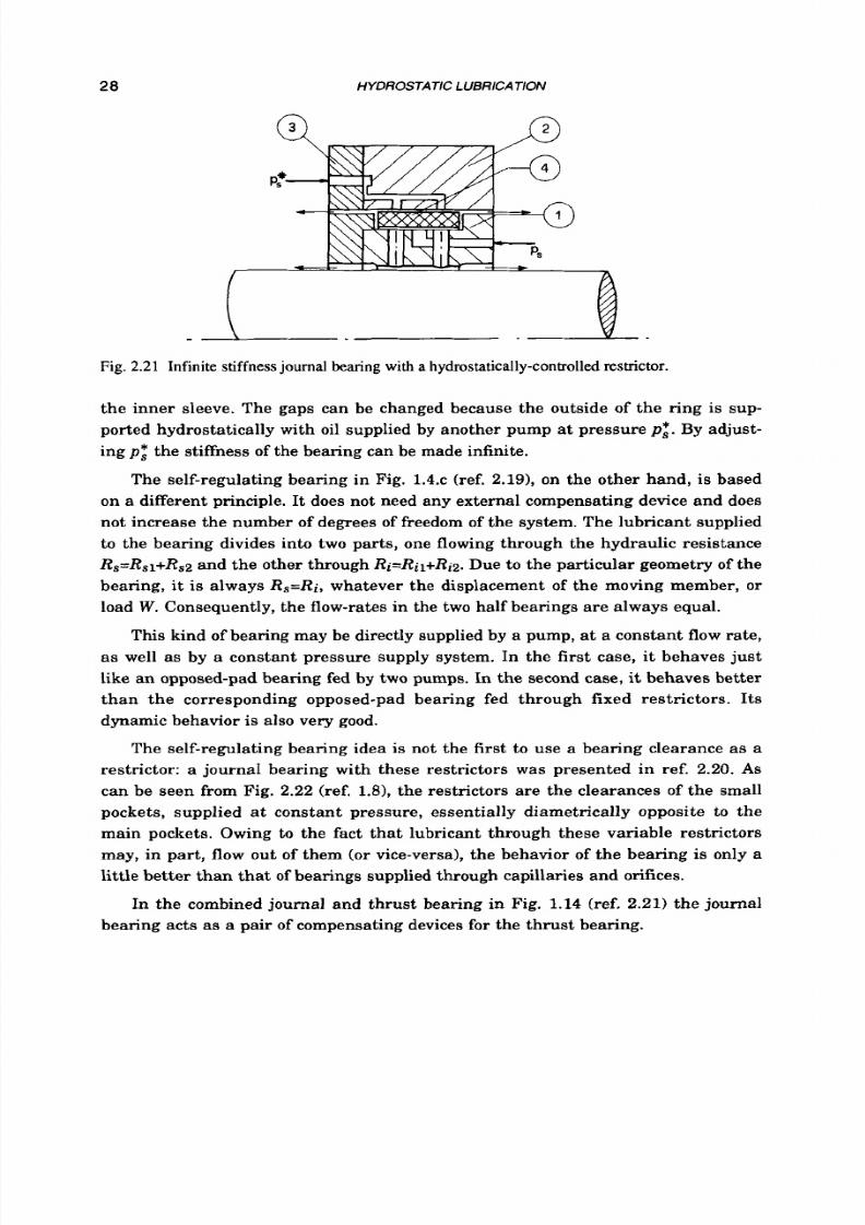
8/9/2019 Hydrostatic Lubrication 1992
http://slidepdf.com/reader/full/hydrostatic-lubrication-1992 45/558
28
HYDROSTATIC LUBRICATION
Fig.
2.21
Infinite stiffness
journal
bearing
with
a
hydrostatically-controlled resmctor.
the inner sleeve. The gaps can be changed because the outside of the ring is sup-
ported hydrostatically with oil supplied by another pump at pressure
p : .
By adjust-
ing p t the stiffness of the bearing can be made infinite.
The self-regulating bearing in Fig. 1.4.c (ref. 2.191, on the other hand, is based
on a different principle. It does not need any external compensating device and does
not increase the number of degrees of freedom of the system. The lubricant supplied
t o
the bearing divides into two parts, one flowing through the hydraulic resistance
Rs=Rsl+Rs2and the other through
Ri=Ril+Riz.
Due to the particular geometry of the
bearing, it is a lways
R s= R i ,
whatever the displacement of the moving member, o r
load W. Consequently, the flow-rates in the two half bearings are always equal.
This kind of bearing may be directly supplied by a pump, at a constant flow rate,
as well as by a constant pressure supply system. In the first case,
it
behaves just
like a n opposed-pad bearing fed by two pumps. In
the
second case, it behaves better
than the corresponding opposed-pad bearing fed through fixed restrictors. Its
dynamic behavior
is
also very good.
The self-regulating bearing idea
is
not the first to use a bearing clearance as a
restrictor: a journal bearing with these restrictors was presented in ref. 2.20. As
can be seen from Fig. 2.22 (ref. 1.81, the restrictors a re the clearances of the small
pockets, supplied at constant pressure, essentially diametrically opposite to the
main pockets. Owing to the fact that lubricant through these variable restrictors
may, in part, flow out of them (or vice-versa), the behavior of the bearing is only a
little better than th at of bearings supplied through capillaries and orifices.
In the combined journal and thrust bearing in Fig. 1.14 (ref. 2.21) the journal
bearing acts as a pair of compensating devices for the thrust bearing.

8/9/2019 Hydrostatic Lubrication 1992
http://slidepdf.com/reader/full/hydrostatic-lubrication-1992 46/558
COMPENSATlNG DEVICES
29
Restrictor
lands
N o 4 N o 3 N O 1
N o 2
A ,
I I
I I
I I
I
1
Main
N o 2 No3 Gmove Supply
~ o 4
restr ictor hole
o 1
Fig.
2.22
Developed view of a hydrostatic journal bearing having integral variable restrictors.
2.3.4
Reference bear ings
A
small bearing
r
in Fig. 2.23, compensated by a diaphragm valve, has been
proposed (ref. 2.6)
t o
control the behavior of the large main bearing m by means of a
spool relay s. The positioning accuracy of the main bearing
is
the same as the accu-
rately manufactured and positioned "reference" bearing, and it s stiffness is very
high.
- a - - b -
Fig.
2.23
Reference bearing:
a-
beitring r controls the main bearing m by means of a diaphragm
valve v and a relay s; b- the reference bearing
is
an interface restrictor bearing ri. and the diaphragm
valve is controlled by a solenoid.
8/9/2019 Hydrostatic Lubrication 1992
http://slidepdf.com/reader/full/hydrostatic-lubrication-1992 47/558
3 0 HYDROSTATIC LUBRICA TlON
A bearing which seems particularly suitable for use
as
a reference bearing is
the "interface restrictor bearing" (ref. 2.22) shown in Fig. 2.23.b. It is enclosed by
flat washer (made from low friction material) that prevents leakage of the lubricant,
which flows radially
t o
the central hole. The bearing may be supplied by a di-
aphragm valve, and this feature allows it to operate at large gaps with great stiff-
ness and accuracy. Especially if external controlling force is operated by a solenoid,
the bearing becomes an effective reference bearing.
2.4 THE COMMONEST SUPPLY SYSTEMS
2.4.1 Direct supply
Systems provided with a separate motor-pump (usually axial
or
radial piston-
pumps) for each recess (Fig. 2.2) are not very often encountered, because of the rele-
vant plant (and maintenance) costs. It is more common to find plants in which the
pumps are driven by a single motor (as in Fig. 2.3), o r are linked together to form a
flow-divider, as in Fig. 2.4. The cost of these systems are lower, while at the same
time maintaining the same performance, i.e. high load capacity and stiffness, and
greater eficiency than in the case of the other types of supply systems.
A
certain use may be foreseen for the self-regulating bearings (Fig.l .4) as well
as of
systems of self-regulating pads (ref.
2.23)
and self-regulating screw and nut
assemblies (Fig. 1.lO.b) for their high load capacity and stiffness, and not high cost.
2.4.2 Compensated supply
(i)
Fired restrictors. The most common fixed restrictors are laminar-flow re-
strictors, especially capillary tubes. They are easy t o find o r to build, and hence
cheap. Hypodermic needles are sometimes used as capillaries, as well as many
types of small-diameter pipes of adequate length. Furthermore, their design is very
simple, since their hydraulic resistance is proportional
to
their length (provided the
lat ter is some tens times greater than the diameter).
On the contrary, there are bigger problems with the use of orifices, because
their diameter is generally very small: apart from the fact they tend to be easily
obstructed, this means a great sensitivity to manufacturing tolerances. Further-
more, in the case of the orifices, the system is more sensitive t o any change in the
temperature (i.e. in the viscosity) of the lubricant.
(ii) Var iable restrictors. Constant flow valves are sometimes used, even though
they are somewhat complicated and costly devices. The reason is that they are easily
available and widely used in many oilhydraulic plants.
8/9/2019 Hydrostatic Lubrication 1992
http://slidepdf.com/reader/full/hydrostatic-lubrication-1992 48/558
COMPENSATING
DE
lCES 31
For almost all the other controlled restrictors experimental applications are
known (chapter
14).
Diaphragm flow dividers, in particular, have been widely stud-
ied in connection with opposed-pad bearings, journal bearings, hydrostatic slide-
ways and screw-nut assemblies.
A
wider use of such devices
is
recommended,
since they are simple to build and their performance is excellent.
(iii) Inherently compensated bearings. For almost all inherently compensated
bearings only experimental applications are known.
2.5 HYDRAULIC CIRCUIT
Figure 2.24.a contains the layout of the hydraulic circuit of a hydrostatic system
supplied at constant pressure. The system in the figure is made up of one
( o r
more)
opposed-pad bearing.
A
pump P driven by a motor
M
pushes the lubricant from the reservoir Sm in
the intake line, in which pressure is kept constant by a relief-pressure valve V,
which discharges the surplus lubricant. The lubricant, passed through a filter F,
arrives at the pads through the restrictors R, which should be as near as possible to
the pads
for
good dynamic behavior of the bearing. The lubricant then flows from
the bearing to the collector S and from this to the reservoir S m .
Besides filter
F,
a strainer may be put a t point [l].After filter
F
a pressure
gauge measures supply pressure
p s . A
pressure-sensing emergency switch is
generally put a t the same point
[ Z ] ,
which may, for instance, switch off the motor
driving the moving members of the bearings if a pressure-drop occurs. An accumu-
lator, preceded by a a check valve Vn, an supply the system during
its
inertia
movements. Pressure gauges may be put after the restrictors to indicate the pres-
sures in the recesses, but they should be switched
off
during running for good
dynamic behavior of the bearing. If the gravity discharge is not sufficient, ever in
large pipes, an exhaust pump may be inserted a t point [4].
As will be explained more extensively later, lubricant is heated in the circuit,
and especially in restrictors and in the bearing pads, as a consequence of viscous
friction.
So,
if natural cooling in the reservoir is not sufficient, a cooler may be in-
serted at point
[5],
or a t point [l] f a close temperature control is required. The
cooler may also be put in parallel t o the reservoir. Thermometers T are generally
inserted in the circuit, in particular after the cooler [5]. A temperature transducer,
located a t point [3], may switch off the driving motor if temperature exceeds the ad-
missible value.
If pads are provided externally with low-friction seals, a low pressure at the
film exit may pump the return lubricant directly t o reservoir
S m ,
thereby simplify-
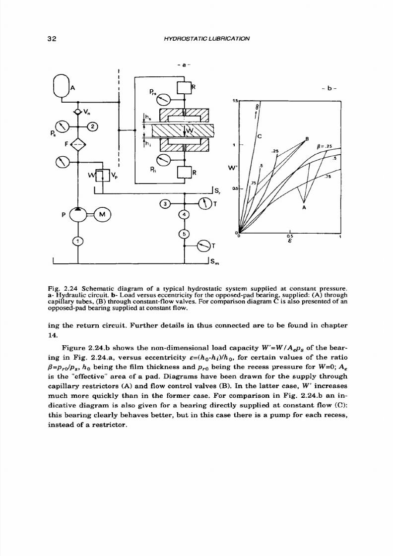
8/9/2019 Hydrostatic Lubrication 1992
http://slidepdf.com/reader/full/hydrostatic-lubrication-1992 49/558
32
HYDROSTATIC LUB RICATlON
- a -
&
I
I
1
W
a
-
b -
a5
&
Fig. 2.24 Schematic diagram of a typical hydrostatic system supplied at constant pressure.
a-
Hydraulic circuit.
b-
Load versus eccentricity
for the
opposed-pad bearing, supplied:
(A)
through
capillary tubes,
(B)
through constant-flow valves. For comparison diagram C is also presented of an
opposed-pad bearing supplied at constant flow.
ing the return circuit. Further details in thus connected are to be found in chapter
14.
Figure 2.24.b shows the non-dimensional load capacity W'=W/Ag, of the bear-
ing in Fig. 2.24.a, versus eccentricity
E=(ho-hi)lho,
or certain values of the ratio
P=p,dp,, ho
being the film thickness and p r o being the recess pressure for W=O; A,
is the "effective" area of a pad. Diagrams have been drawn for the supply through
capillary restrictors (A) and flow control valves (B). In the latter case,
W'
increases
much more quickly than in the former case. For comparison in Fig. 2.24.b an in-
dicative diagram is also given for a bearing directly supplied a t constant flow
( C ) :
this bearing clearly behaves better, but in this case there is a pump
for
each recess,
instead
of
a restrictor.
8/9/2019 Hydrostatic Lubrication 1992
http://slidepdf.com/reader/full/hydrostatic-lubrication-1992 50/558
COMPENSATING DEVICES
33
REFERENCES
2.1
2 6
2.3
2.4
2.6
2.6
2.7
2.8
2 9
2.10
2.11
2.12
2.13
2.14
2.16
2.16
2.17
2.18
Siebers
G.; Hydrostatische Lagerungen und Fiihrungen; Verlag Technische
Rundschau, Bern, 1971; 75 pp.
Kundel K., Arsenius T.; Cuscinetti Idrostatici; Rivista dei Cuscinetti-SKF',47
(19721, 1-8.
Opitz H.; Pressure Pad Bearings; Proc. Instn. Mech. Engrs., 182,3A (1967-681,
100-115.
Wiener H.;
The Plastic Throttle - a Novel Component for Hydrostatic Slid ing
Bearings; Ball and Roller Bearing Engineering-FAG, 1974, N. 2; pp. 41-44.
Morsi S. A.; Tapered Spool Controller for Pressurized Oil Film Bearings;
Proc. Instn. Mech. Engrs., 184,l (1969-701,387-396.
Mohsin M. E.; The Use of Controlled Restrictors for Compensating Hydro-
static Bearings;
Advances in Mach. Tool Des. and Res., Proc. 3rd Int. MTDR
conf,, Birmingham, 1962; pp. 429-442.
Merritt H. E.; Hydraulic Control Systems;
J o h n
Wiley &
Sons,
N. Y., 1967; 350
PP.
Royle J. K., Howarth R. B., Casely A. L.; Applications of Automatic Control to
Pressurized Oil Film Bearings; Proc. Instn. Mech. Engrs., 176,22 (19621, 532-
541.
Mayer J. E., Shaw
H.
C.; Characteristics
of
a n Externally P ressurized B ear-
ing Having Variable External Flow Restrictors; ASME Trans.,
J . of
Basic
Engineering,
86
(19631,291-296.
Bassani R.;
Divisore di Flusso a Spola C onica: sua Applicazione a Su pp orti
Idrosta t ic i ; Fluid-Apparecchiature Idrauliche e Pneumatiche, l S,17 1-172
De
Gast
J. G. C.; A New Type of Controlled Restrictor (M.D.R.) for Double
Film Hydrostatic Bearings and its
Application to High-Precision M achine
Tools;
Advance in Mach. Tool Des. and Res., Proc. of the 7th
Int.
MTDR Conf.,
Birmingham, 1966; pp. 273-298.
O'Donoghue J. P., Hooke C. J.; Design of Inherently Stable Hydrostatic Bear-
ings; Proc. Instn. Mech. Engrs., Tribology Convention, 1969.
Hirs G. G.; Partly Grooved Externally Pressurized Be arin gs; Proc. Instn.
Mech. Engrs., Lubrication and Wear Convention, 1966; paper 21.
Dowson D., Taylor C. M.; Elastohydrostatic of Circular Plate Thrust Bear-
ings; ASME Trans., J. of Lubrication Technology,89 (19671,237-262.
Davies P. B.; Investigation of a n All-Metallic Flexible Hydrostatic Th ru st
Bearing; ASLE Trans., 17 (19741, 117-126.
Tully N.; Static and Dynamic Performance of a n Infin ite Stiffness H ydrostatic
Thrust Bearing; ASME Trans.,
J. of
Lubrication Technology, 99 (19771, 106-
112.
Brzeski L., Kazimierski
2.;
High Stiffness Bearing;
ASME Trans.,
J.
of Lu-
brication Technology,
101
(19791,520-525.
Mizumoto H., Kubo M., Makimoto
Y.,
Yoshimochi
S.,
Okamura
S.,
Matsubara T.;
A
Hydrostatically-Controlled Restrictor for Infinite Stiffness
Hydrostatic Journal Bearing; Bull. Japan Soc. of Precision Eng., 21 (19871, 49-
54.
(19781,31-37.

8/9/2019 Hydrostatic Lubrication 1992
http://slidepdf.com/reader/full/hydrostatic-lubrication-1992 51/558

8/9/2019 Hydrostatic Lubrication 1992
http://slidepdf.com/reader/full/hydrostatic-lubrication-1992 52/558
Chapter 3
LUBRICANTS
3.1
INTRODUCTION
Lubricants are put between two surfaces t o prevent direct contact. They may be
subdivided into solid lubricants and fluid lubricants.
Fluid lubricants are used in hydrostatic lubrication; these may be subdivided
into liquid lubricants and gaseous lubricants. Of the two, liquid lubricants are more
frequently employed, including water, also utilized in the first hydrostatic experi-
ments (ref.
1.1),
and liquid metals, especially sodium. But the liquid lubricants most
often employed are mineral lubricants. Nowadays synthetic lubricants are also
used.
Mineral lubricants are obtained from the distillation and refining processes of
crude petroleum, which is separated into fractions of progressively decreasing
volatility, with the elimination of the unwanted ones. Mineral oils are made up of
hydrocarbons, i.e., compounds
of
hydrogen and carbon.
Synthetic lubricants are produced by the substantial chemical modification of
raw materials, which may also be obtained from crude petroleum.
Mineral lubricants are mainly used in hydrostatic lubrication.
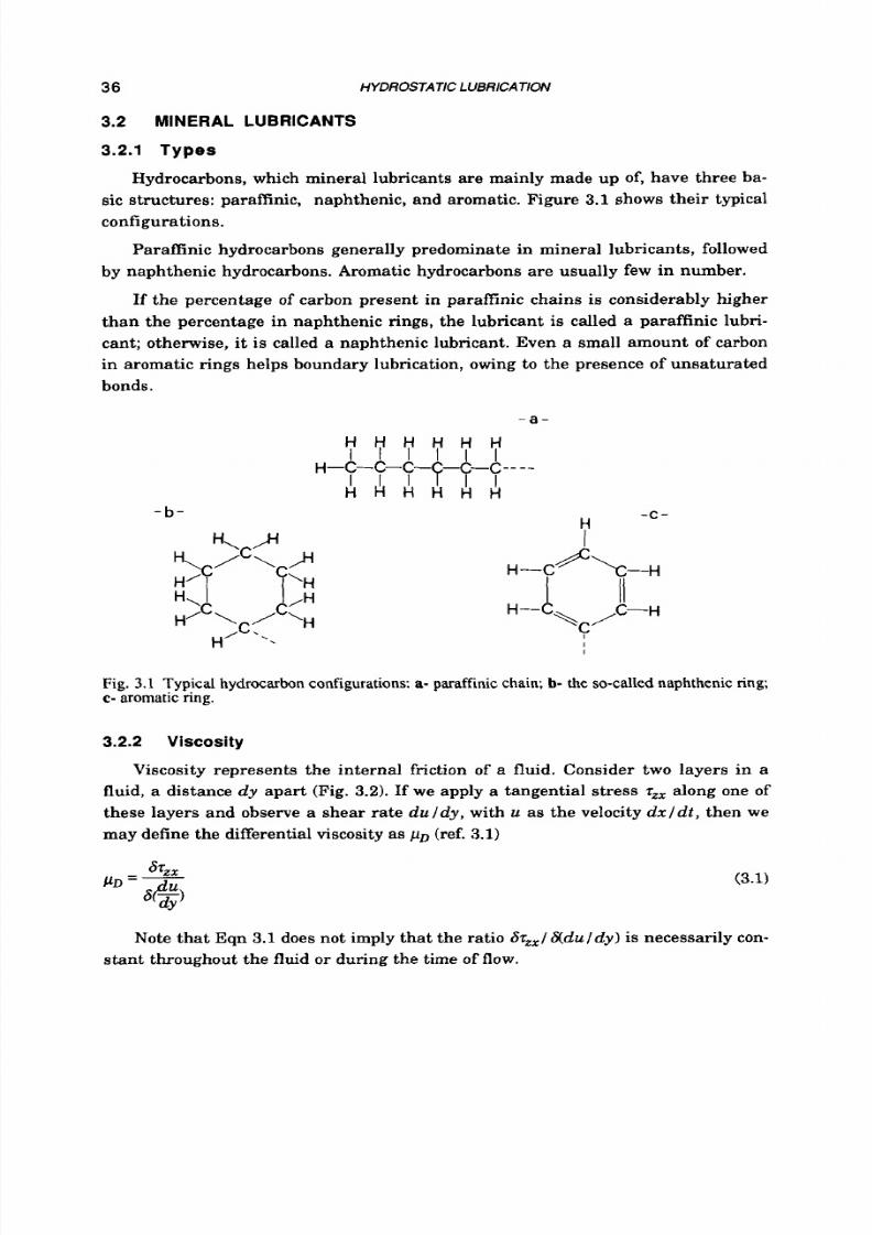
8/9/2019 Hydrostatic Lubrication 1992
http://slidepdf.com/reader/full/hydrostatic-lubrication-1992 53/558
36 HYDROSTATIC LUBRICATION
3.2 MINERAL LUB RICANTS
3.2 .1 Types
Hydrocarbons, which mineral lubricants are mainly made up of, have three ba-
sic structures: paraffinic, naphthenic, and aromatic. Figure 3.1 shows their typical
configurations.
Paraffinic hydrocarbons generally predominate in mineral lubricants, followed
by naphthenic hydrocarbons. Aromatic hydrocarbons are usually few in number.
If the percentage of carbon present in paraffinic chains is considerably higher
than the percentage in naphthenic rings, the lubricant is called a paraffinic lubri-
cant; otherwise, it is called a naphthenic lubricant. Even a small amount of carbon
in aromatic rings helps boundary lubrication, owing
to
the presence
of
unsaturated
bonds.
- a -
- b -
-C -
H
I
I
Fig.
3.1
Typical hydrocarbon configurations:a- paraffinic chain;
b-
the so-called naphthenic ring;
c- aromatic ring.
3.2.2 Viscosity
Viscosity represents the internal friction of a fluid. Consider two layers in a
fluid, a distance
dy
apart (Fig. 3.2) . If we apply a tangential stress z along one of
these layers and observe
a
shear rate
d u d y ,
with u as the velocity
d x l d t ,
then we
may define the differential viscosity
as
p~ (ref. 3.1)
Note that Eqn 3.1 does not imply that the ratio
6 zZ x /& d u d y )
s necessarily con-
stant throughout the fluid
or
during the time
of flow.
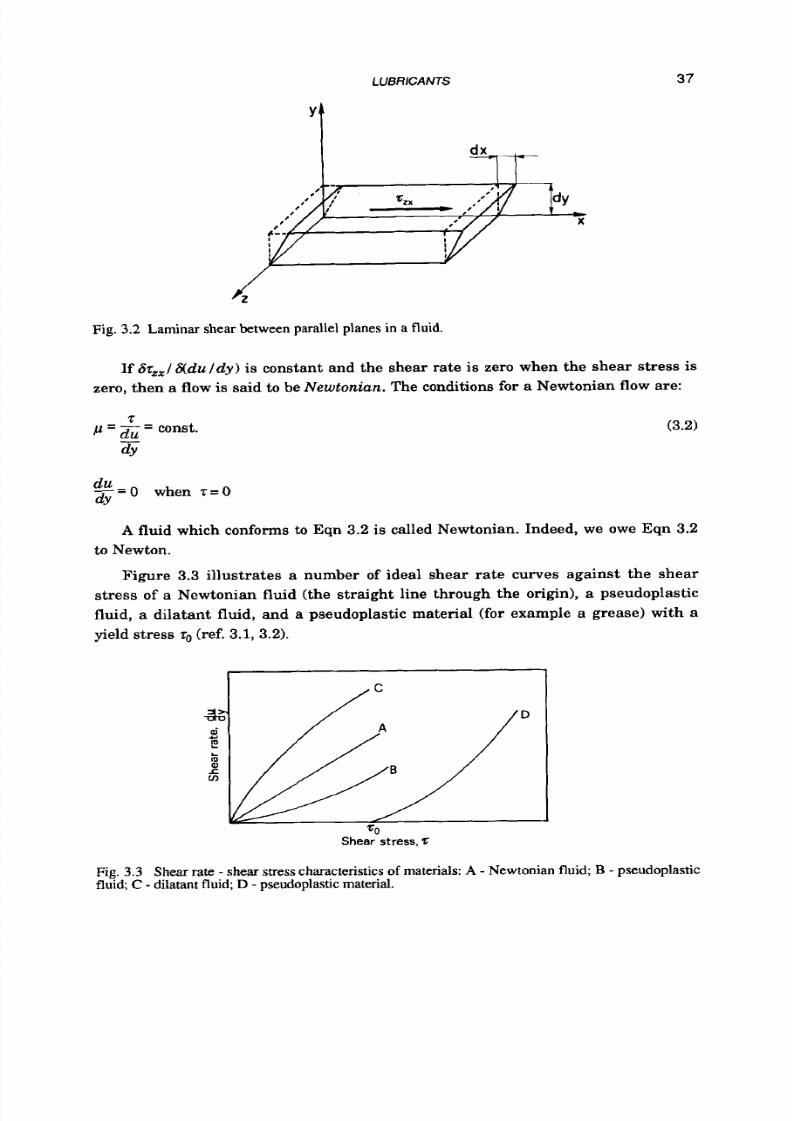
8/9/2019 Hydrostatic Lubrication 1992
http://slidepdf.com/reader/full/hydrostatic-lubrication-1992 54/558
LUBRICANTS
37
Fig.
3.2
Lam inar shea r between parallel planes in
a
fluid.
If
Sz,,/
& du l d y ) is constant and the shear rate is zero when the shear stress is
zero, then a flow is said to be Newtonian. The conditions for a Newtonian flow are:
(3.2)
d u = O
when z = O
dY
A fluid which conforms to Eqn 3.2 is called Newtonian. Indeed, we owe Eqn 3.2
to Newton.
Figure
3.3
illustrates a number of ideal shear rate curves against the shear
stress of a Newtonian fluid (the straight line through the origin),a pseudoplastic
fluid, a dilatant fluid, and a pseudoplastic material (for example a grease) with
a
yield
stress
(ref.
3.1, 3.2).
I
Shear
stress,Z
Fig.
3.3
Shear rate - shear stress characteristics of materials: A
-
Newtonian fluid;
B
- pseudoplastic
fluid;
C
-
dilatant fluid;
D
- pseudop lastic material.

8/9/2019 Hydrostatic Lubrication 1992
http://slidepdf.com/reader/full/hydrostatic-lubrication-1992 55/558
3 8 HYDROSTATIC LUBRICATION
Parameter p, defined by Eqn 3.2, is called dynamic viscosity. In system SI its
unit is Ndm2 or Pas, in system c.g.s. it is dynes/cm2o r poise.
Mineral lubricants and synthetic lubricants of low molecular weight are Newto-
nian in many practical working conditions.
In many fluid flow problems the ratio
(3.3)
is used, where p is the density of the fluid, v is the kinematic viscosity,
its SI
unit is
m2/s and
its
c.g.s. unit is cm2/s or Stoke
(St).
In selecting a n oil for a given application, viscosity
is
a primary consideration,
especially from the point of view of its change with temperature. Various systems
are used to classify and identify oils according
t o
viscosity ranges, including the
"Viscosity system for Industrial Fluid Lubricants", devised by IS0 (Std 3448) nd
now coming into wide use. Viscosity systems establish a series of definite viscosity
levels as a common basis for specifying the viscosity of industrial fluid lubricants.
Reference viscosities are measured in mmVs
o r
cSt (centistokes) at the reference
temperature of 40°C.The viscosity ranges and the corresponding marks t o classify
oils are shown in Table 3.1, for
v=5.06+242
cSt. For comparison, the partial S A E
(Society of Automotive Engineers) classification is also shown. The reference tem-
perature of the SAE classification
is
lOO"C, nd sUmx W is intended for use in cases
where low ambient temperature is encountered.
TABLE 3.1
Viscosity System
for
Industrial Fluid Lubricants.
I
Viscosity System Grade Mid-Point viscosity Kinematic viscosity
Classification cSt (m 2 /s )a t 40°C limits
and Identification cSt (mm%)at 40°C
Min
Max
I S 0
VG 5 4.6 4.14 5.06
IS0 VG 7 6.8 6.12 7.48
ISOVG 10 10 9 .0 11.0
I S 0
VG 15
15
13.5 16.5
I S 0 VG 22 22 19.8 24.2
I S 0 VG 32 32 28.8 35.2
I S 0
VG 46 46 41 .4 50.6
I S 0
VG 68 68 61 .2
74.8
I S 0
VG
100
100 90.0
110
I S 0 VG 150 150 135 165
I S 0
VG
220 220 198 242
S A E
Classification
5w
low
2 0 w
30
50
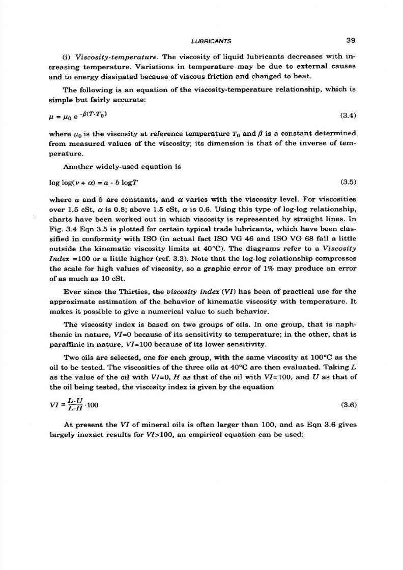
8/9/2019 Hydrostatic Lubrication 1992
http://slidepdf.com/reader/full/hydrostatic-lubrication-1992 56/558
LUBRICANTS 39
(i) Viscosity-temperature. The viscosity of liquid lubricants decreases with in-
creasing temperature. Variations in temperature may be due t o external causes
and to energy dissipated because of viscous friction and changed to heat.
The following is an equation of the viscosity-temperature relationship, which is
simple but fairly accurate:
(3.4)
where po is the viscosity at reference temperature
To
and
p
is a constant determined
from measured values of the viscosity; it s dimension is that of the inverse of tem-
perature.
Another widely-used equation is
log log(v+ a)= a -
b
logT
(3.5)
where a and b are constants, and a varies with the viscosity level. For viscosities
over 1.5 cSt, a is
0.8;
above 1.5 cSt, a is
0.6.
Using this type of log-log relationship,
charts have been worked out in which viscosity is represented by straight lines. In
Fig.
3.4
Eqn
3.5
is plotted for certain typical trade lubricants, which have been clas-
sified in conformity with IS0 (in actual fact IS0 VG
46
and
IS0 VG 68
fall a little
outside the kinematic viscosity limits at
40°C).
The diagrams refer
t o
a Viscos i ty
Index =lo0
o r
a little higher (ref. 3.3).Note that the log-log relationship compresses
the scale for high values of viscosity,
so a
graphic error of 1% may produce an error
of as much as 10 cSt.
Ever since the Thirties, the viscosity index ( V n has been of practical use for the
approximate estimation of the behavior of kinematic viscosity with temperature. It
makes i t possible to give a numerical value t o such behavior.
The viscosity index is based on two groups
of oils.
In one group, that is naph-
thenic in nature, VZ=O because of its sensitivity t o temperature; in the other, that is
paraffinic in nature, VZ=100 because of its lower sensitivity.
Two oils are selected, one for each group, with the same viscosity at
100°C
as the
oil
t o be tested. The viscosities of the three oils at
40°C
are then evaluated. Taking L
as the value of the oil with VI=O,
H
as that of the oil with VI=lOO, and
U
as that of
the oil being tested, the viscosity index
is
given by the equation
L -
u
vz= ---loo
L - H
(3.6)
A t
present the
VZ
of mineral oils is often larger than
100,
and
as
Eqn
3.6
gives
largely inexact results for VZ>lOO, an empirical equation can be used:
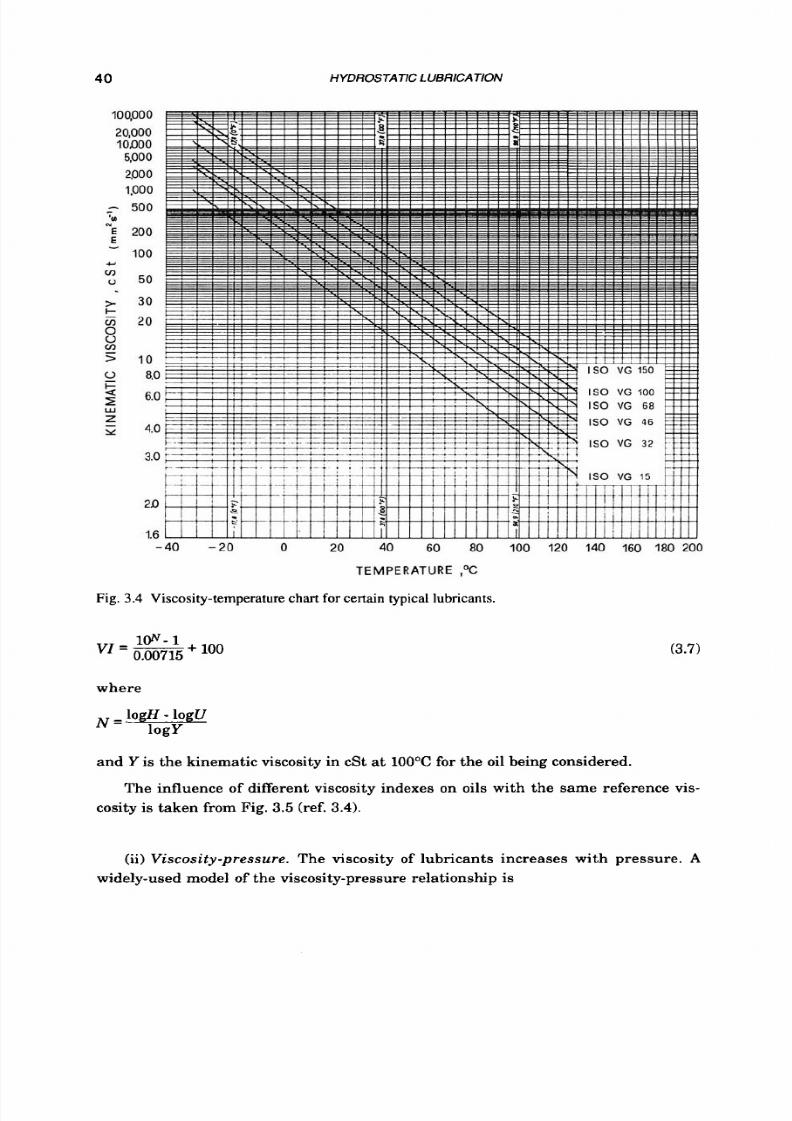
8/9/2019 Hydrostatic Lubrication 1992
http://slidepdf.com/reader/full/hydrostatic-lubrication-1992 57/558
40
HYDROSTATIC LUBRICATION
Fig.
3.4
Viscosity-temperature chart for certain typical lubricants.
VI = lW -
+
100
0.00715
(3.7)
where
logH
-
l0gU
N = logy
and Y is the kinematic viscosity in cSt at 100°C for the oil being considered.
The influence of different viscosity indexes on oils with the same reference vis-
cosity is taken from Fig. 3.5 (ref. 3.4).
(ii)
Viscos i ty -pressure .
The viscosity of lubricants increases with pressure. A
widely-used model of the viscosity-pressure relationship is
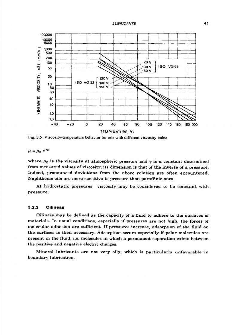
8/9/2019 Hydrostatic Lubrication 1992
http://slidepdf.com/reader/full/hydrostatic-lubrication-1992 58/558
LUBRICANTS
41
-40 -20 0 20
40 60
80
100
120
140 160 180
200
TEMPERATURE .Dc
Fig. 3.5 Viscosity-temperaturebehavior for oils with different viscosity index
where
po
is the viscosity at atmospheric pressure and
y
is a constant determined
from measured values of viscosity; its dimension is
that
of the inverse of a pressure.
Indeed, pronounced deviations from the above relation are often encountered.
Naphthenic oils are more sensitive to pressure than paraffinic ones.
A t
hydrostatic pressures
viscosity may be considered
t o
be constant with
pressure.
3.2.3 Oiliness
Oiliness may be defined as the capacity of a fluid to adhere t o the surfaces of
materials. In usual conditions, especially if pressures are not high, the forces of
molecular adhesion are sufficient. If pressures increase, adsorption of the fluid on
the surfaces is then necessary. Adsorption occurs especially if polar molecules are
present in the fluid, i.e. molecules in which a permanent separation exists between
the positive and negative electric charges.
Mineral lubricants are not very oily, which is particularly unfavorable in
boundary lubrication.
8/9/2019 Hydrostatic Lubrication 1992
http://slidepdf.com/reader/full/hydrostatic-lubrication-1992 59/558
42 HYDROSTATIC LUBRICATION
3.2.4
Densi ty
As is well known, the density of a liquid is the mass of a unit volume, generally
calculated at 15°C. In paraffinic mineral oils p=0.85-0.89 kgfdm3; in naphthenie
mineral oils p=0.90-0.93 kg/dm3. Density varies with temperature and with
pressure.
(i) Thermal expansion. For a liquid, thermal expansion can be defined as the
property of being changed in density with temperature.
It
can be stated approxi-
mately by the equation
p(T) = po 11- a ( T -To)]
(3.8)
where
a
increases as p decreases; approximately: a=4.1.10-4
+
8.2.10-40C-1 or
p=0.22+0.01 Ns/m2.
In hydrostatic lubrication thermal expansion is often negligible.
(ii) Compressibil i ty . The compressibility of a liquid can be defined a s the prop-
erty of being changed in density with pressure:
(3.9)
Compressibility can also be expressed as a change in volume with pressure; indeed,
if V is the volume (of a mass
M)
f liquid, then from Eqn 3.9
1 d V
c = - - -
v dP
(3.10)
Compressibility changes with pressure and temperature; it also changes with
molecular structure, but cannot be changed by means of additives, since it is a phys-
ical property of the base liquid.
Very often, instead of compressibility, its reciprocal is used: the bulk modulus
KL. igure
3.6
(ref. 3.4) shows
a
method for predicting the bulk modulus of mineral
oils:
1) with density pT calculated a t ambient pressure (105 Pa) and a t the desired
temperature
T,
Fig. 5.6.a defines the bulk modulus at pressure 1380.105
Pa;
2) with this bulk modulus enter into Fig. 3.6.b: a vertical line
at
the intersec-
tion with the 1380.105 Pa line gives the modulus a t any other pressure
and
at
the selected temperature.
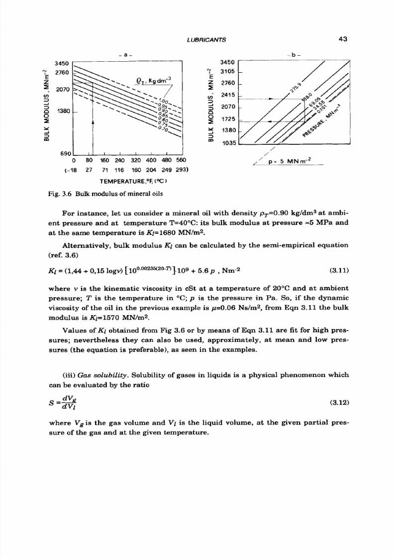
8/9/2019 Hydrostatic Lubrication 1992
http://slidepdf.com/reader/full/hydrostatic-lubrication-1992 60/558
LUBRlCANTS 43
- a - - b -
690
0 80 160 240 320 400 480 560
(-18 27 71 116 160 204 249 293)
TEMPERATUREFF, (OC)
Fig. 3.6 Bulk modulus of
mineral
oils
3450
3105
E
5
2760
cn-
2415
2
2070
n
p 1725
5 1380
1035
3
/
/
/'
p =
5
M N ~
For instance, let us consider a mineral oil with density p,=0.90 kg/dm3
at
ambi-
ent pressure and at temperature
T=40°C:
ts bulk modulus a t pressure -5 MPa and
at the same temperature is
K1=1680
MN/m2.
Alternatively, bulk modulus KLcan be calculated by the semi-empirical equation
(ref.
3.6)
K1= (1,44 + 0,15
logv)
[10°.00235(20-n].1095.6p ,
Nm-2
(3.11)
where
v
is the kinematic viscosity in cSt at a temperature of
20°C
and at ambient
pressure; T
is
the temperature in
"C;p is
the pressure in Pa. So, if the dynamic
viscosity of the oil in the previous example is
p 0 . 0 6
Ns/m2, from Eqn
3.11
the bulk
modulus is
K2=1570MN/m2.
Values of
K1
obtained from Fig
3.6
or by means of Eqn
3.11
are
fit
for high pres-
sures; nevertheless they can also be used, approximately,
at
mean and low pres-
sures (the equation is preferable), as seen in the examples.
(iii)Gas
solubility.
Solubility of gases in liquids is a physical phenomenon which
can be evaluated by the ratio
(3.12)
where Vgis the gas volume and Vi is the liquid volume, at the given partial pres-
sure of the gas and at the given temperature.

8/9/2019 Hydrostatic Lubrication 1992
http://slidepdf.com/reader/full/hydrostatic-lubrication-1992 61/558
4 4 HYDROSTATIC LUBRICATION
Solubility varies with pressure and temperature. In Fig. 3.7.a solubility of air
versus pressure is shown in a mineral oil (Mil-h-5606A) and in other liquids (ref.
3.5). Also at higher temperatures air solubility varies almost linearly. Figure 3.7.b
shows solubility versus temperature in the case of certain gases in
a
mineral oil
with p=850 kg/m3
The air dissolved m a y affect lubricant properties, such as viscosity which grows
worse. The air dissolved in an oil comes out of solution when temperature and pres-
sure decrease and may produce air bubbles and foam.
- a -
- b -
MINERAL
OIL
0 2 4 6 8 1 0
0 25 50 75 100 125
PRESSURE, MP a TEMPERATURE PC
Fig. 3.7
Solubility
of
gase s versus: a- pressure; b- temperature.
(iv)Air entrainment. Common causes
of
entrained air in a liquid are, for ex-
ample, leaks in the pump suction or when the return line discharges liquid above
its surface level in the reservoir.
In any case, air is inevitably taken into a mineral oil as it passes into a lubricat-
ing system
so
that the oil in the reservoir may contain as much as 15%of dispersed
air (ref. 3.7). In a large and suitable reservoir this air should be given up and re-
duced, after a fairly long time, t o about 1.5%, and after a very long time t o about
0.5%. But the air bubble content is rarely reduced to the desired levels.
Air bubbles, when compressed, go into solution, but not immediately. In Fig.
3.8, the percentage of air bubbles dissolved in a hydraulic oil is shown as a function
of time, for certain pressures (ref. 3.5). We see,
for
example, that for p=3 MPa, after
1
second, less than 10%of the air bubbles go into solution. Thus, as a result
of
the oil
velocity in the supply lines of hydrostatic systems (0.5t50
m/s
and even more), these
percentages are generally
low.

8/9/2019 Hydrostatic Lubrication 1992
http://slidepdf.com/reader/full/hydrostatic-lubrication-1992 62/558
LUBRICANTS
45
40
0
1
2 3
4
5
T I M E
, s
Fig 3.8 Rate
of solution
of
air bubbles
in
a mineral oil.
Air viscosity is low, i.e. p=1.78.10-6 Ns/m2 a t l0C and 0,981.105 Pa; therefore,
entrained air affects the viscosity
of
oils. Fortunately, the effect
is
relatively slight,
and can be expressed by the empirical relation
clp = (1+ 0.015 B )
where
B is
the percentage of bubble content,
p o
the viscosity of
oil
and pb the effective
viscosity of bubbly oil.
The air bulk modulus is also low, so the entrained air affects the actual bulk
modulus
of
oils. The equation of state of a perfect gas (to which air may be assimi-
lated)
for
an adiabatic process
( to
which the compression of air bubbles in mineral
oils may be compared) is
p VCP'~V
= const. (3.13)
where cp and c v are the specific heats a t constant pressure and constant volume,
respectively.
If
Eqn 5.13 s introduced into Eqn 5.10, the bulk modulus Ka
of
air
is
obtained
(3.14)
A t temperature T=40"C and at pressure p=0.981.105 Pa, we have cp=1.0048~103
J/kg"C, and cv=0.717.103 J/kg"C; thus we have cplcv=1.401,and Ka=1.37.105 Pa. In
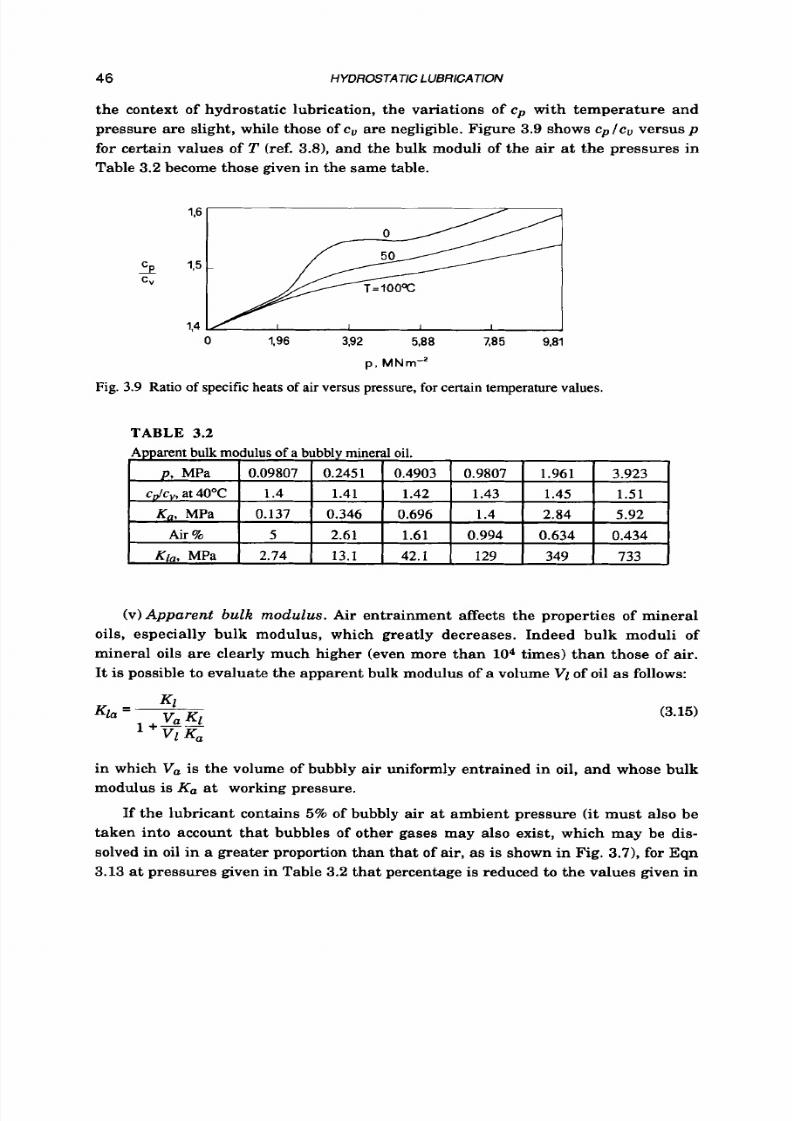
8/9/2019 Hydrostatic Lubrication 1992
http://slidepdf.com/reader/full/hydrostatic-lubrication-1992 63/558
46 HYDROSTATIC L UBRICA
TlON
the context of hydrostatic lubrication, the variations of cp with temperature and
pressure are slight, while those of cv are negligible. Figure 3.9 shows cp/cvversus p
for certain values of
T
(ref. 3.8), and the bulk moduli of the air at
the
pressures in
Table
3.2
become those given in the same table.
0 1,96 3,92
5,aa
7,a5 9,ai
p ,
MNrn-'
Fig. 3.9 Ratio of specific heats of air versus pressure,
for
certain temperature values.
TABLE 3.2
(v) Apparent
bulk modulus. Air
entrainment affects the properties
of
mineral
oils, especially bulk modulus, which greatly decreases. Indeed bulk moduli of
mineral oils are clearly much higher (even more than lo* times) than those of air.
It
is
possible
t o
evaluate the apparent bulk modulus of a volume
Vi
of oil a s follows:
(3.15)
in which
Va
is the volume of bubbly air uniformly entrained in oil, and whose bulk
modulus is
K,
a t working pressure.
If the lubricant contains
5% of
bubbly air at ambient pressure (it must also be
taken into account that bubbles
of
other gases may also exist, which may be dis-
solved in oil in a greater proportion than that
of
air, as
is
shown in Fig.
3.71, or
Eqn
3.13
at
pressures given in Table
3.2
that percentage
is
reduced to the values given in

8/9/2019 Hydrostatic Lubrication 1992
http://slidepdf.com/reader/full/hydrostatic-lubrication-1992 64/558
LUBRlCANTS 47
the same table.
So,
for Eqn 3.15, the apparent bulk moduli given in Table 3.2 may be
assigned to the oil a t those pressures.
The elastic deformation of the supply line may also influence the bulk modulus
of mineral oils. For a circular pipe, the internal pressure ps causes a change in
volume, which should be added to the change in volume due t o the compressibility of
the fluid when evaluating effective compressibility (Eqn 3.10) and hence the appar-
ent bulk modulus. The equivalent bulk modulus of a metallic pipe is, approxi-
mately,
(rs
is the internal radius of the pipe,
ra
is the external one,
E
is the modulus of elas-
ticity and v is the Poisson ratio). Equation 3.15 may then be completed as follows:
(3.16)
For instance, let
us
consider a copper pipe, with ra=6 nun, rs=5 mm, and E=118
GPa, v=0.25; the equivalent bulk modulus of the pipe may be calculated as
Ks=10.2.109 Nlm2. For a steel pipe of the same dimensions, with E=206 GPa, v=0.3,
we have KS=17.6.1O9N/m2.
Generally, values of Ks for metallic pipes are much higher than the apparent
bulk modulus Kla of mineral oils (see Table
3.2) so
their influence may be disre-
garded. The same is not true for flexible pipes (also for high-pressure pipes made of
hard rubber
o r
FTFE with an interwoven sheet of stainless steel) as transpires from
existing experimental results. Figure 3.10.a (ref. 3.9) shows the considerable in-
crease in the inner volume of certain flexible hoses.
Obtaining realistic design values of the apparent bulk modulus of oil in hy-
draulic hoses is quite difficult. Values of Kla in the 70t350 MN/m2 range can be
found in the l iterature. Some results are shown in Fig. 3.10.b (ref. 3.5) or a woven
hose with rs=6.4 mm: the experimental data are clearly scattered. Recent design
practice in relation t o equipment dynamic noise reduction has tended to encourage
the use of hydraulic hoses in fluid power systems. This does not always seem con-
venient in hydrostatic systems, as a way of preventing possible dynamic instability.
Elastic deformations of instruments (manometers), pressure reservoirs
(accumulators) and other elements in the supply line may also influence
the
effec-
tive value of the apparent bulk modulus.

8/9/2019 Hydrostatic Lubrication 1992
http://slidepdf.com/reader/full/hydrostatic-lubrication-1992 65/558
48
48
nJ 4 02:
I
24
-
Y
16-
8 -
HYDROSTATIC LUB RICATlON
"
/
e
-
0 0
o o o
I I I I
- a -
10 15
20
0 4 8 12 16 20
PRESSURE,
MNrn-'
PRESSURE,
MPa
Fig.
3.10
Flexible pipes:
a-
Inner volume variation
(for
unit length) versus pressure; (i) internal
radius
rs=5
mm, rated pressure
pN=26
MPa; (ii)
rs=6.5
mm,
pN=26
MPa; (iii)
rs=5
mm, p ~ = l l
MPa. b- Apparent bulk modulus of lubricant versus pressure: rs=6.4 mm, SAE R2 Hose.
(vi)Foaming. The foaming of a liquid is due to the
air
bubbles tha t collect above
its surface. Common causes of foam are the same, but even greater, as in the case
of entrained
air.
Foam in a lubricating system can cause a decrease in pump efficiency, vibra-
tions, and above all inadequate lubrication.
(vii) Cavitation. In fluid systems "gaseous cavitation" refers to the formation in
the liquid of cavities that may contain air or other gases. "Vaporous cavitation"
refers
t o
the fact that, if pressure is reduced far enough, the liquid will vaporize and
will form vapor cavities (mineral oil vapors may contain volatile fractions
of
lubri-
cants). The vapor pressure of a liquid depends on
its
temperature and decreases
with
it.
A t atmospheric pressure water boils a t 100°C,
so
its vapor pressure is 1.0128
bar; at 21.1"C its vapor pressure is reduced to 0.025 bar. The vapor pressure of
mineral oils is much lower than that of water, typically 6.10-4 bar at 4O O C ; hence
cavitation is less likely to occur in the case
of
these liquids. In Fig. 3.11 the vapor
pressure of certain liquids
is
given as a function of temperature (ref.
3.5).
Cavities are well known to be associated with nucleation centers such as micro-
scopic gas particles
(or
microscopic solid particles which gases join to), and their
development is caused by the rapid growth of these nuclei. Hydraulic liquids used in
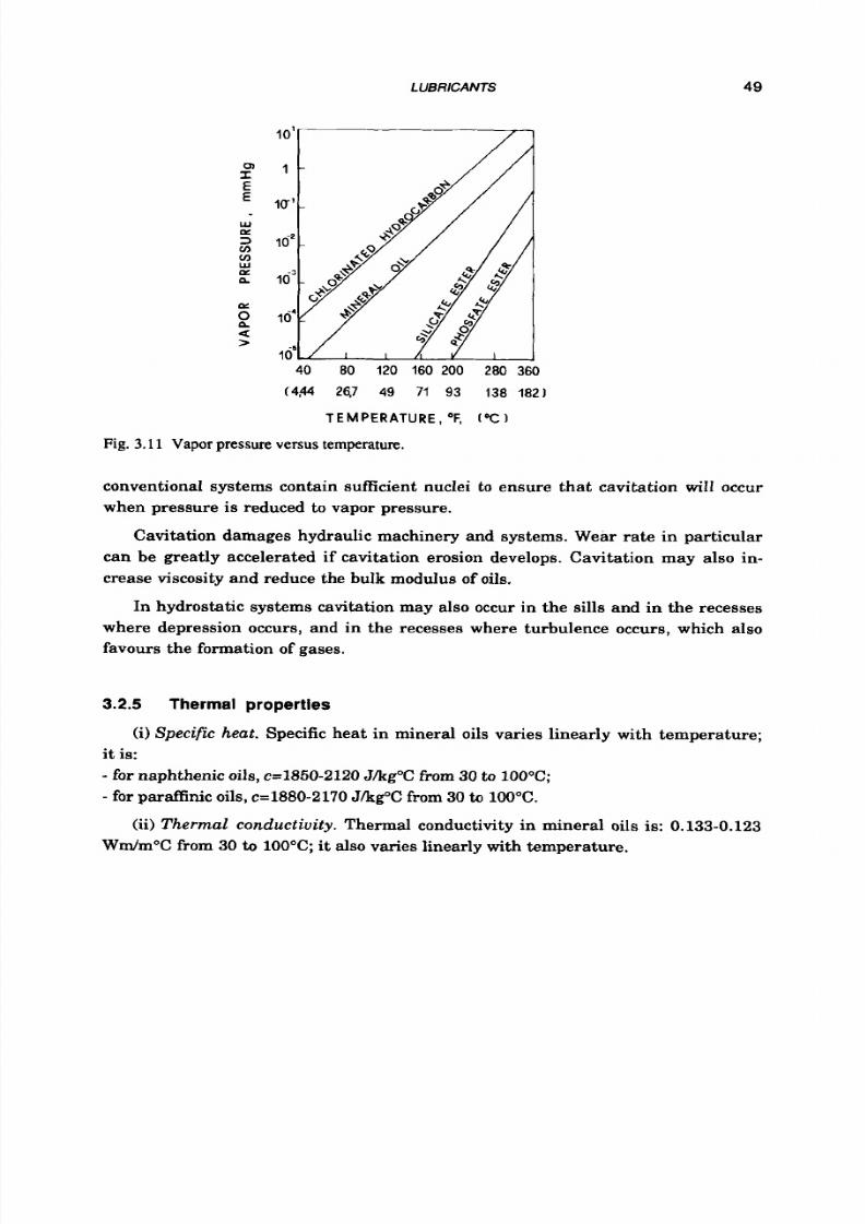
8/9/2019 Hydrostatic Lubrication 1992
http://slidepdf.com/reader/full/hydrostatic-lubrication-1992 66/558
LUBRICANTS
49
i o ' r / 1
0
I
E
E
m
B
a
>
40
80 120 160 200 280 360
(494 26,7 49 71 93 138 1821
TEMPERATURE, OF,
( O C 1
Fig. 3.11 Vapor pressure versus temperature..
conventional systems contain sufficient nuclei t o ensure that cavitation will occur
when pressure
is
reduced to vapor pressure.
Cavitation damages hydraulic machinery and systems. Wear rate in particular
can be greatly accelerated if cavitation erosion develops. Cavitation may also in-
crease viscosity and reduce the bulk modulus of
oils.
In hydrostatic systems cavitation may also occur in the
sills
and in the recesses
where depression occurs, and in the recesses where turbulence occurs, which also
favours the formation of gases.
3.2.5 Thermal propert ies
(i)
Specific heat.
Specific heat in mineral oils varies linearly with temperature;
it is:
- for
naphthenic oils, c=1850-2120 J/kg"C from 30 to 100OC;
- for paraffinic oils, c=1880-2170 J/kg°C from 30 to 100°C.
(ii)Thermal conductiuity.
Thermal conductivity in mineral oils is:
0.133-0.123
Wm/m"C from 30
o
100OC; it also varies linearly with temperature.

8/9/2019 Hydrostatic Lubrication 1992
http://slidepdf.com/reader/full/hydrostatic-lubrication-1992 67/558
5 0 HYDROSTATIC LUBRICATION
3.2.6
Other propert ies
Pour-po in t
is the temperature at which an oil ceases to flow freely. This is
caused by the formation of crystals, mainly of a paraffinic type. The pour-point of
paraffinic oils is a t about
-1O"C,
that
of
naphthenic oils a t about
-40°C.
Flash-point is the lowest temperature at which the vapors given off by an oil
ignite momentarily on the application of a small flame. The flash-point of naph-
thenic oils is a t about 170"C, that of paraffinic oils at about 190°C.
Acidi ty .
Low acidity is advantageous €or reducing corrosion.
Oxida t ion . High stability to oxidation is advantageous, because one cause of
deterioration in lubricant oils is the formation of oxidation products. This also leads
t o
a reduction
of
the life of the lubricant and
to
corrosive effects.
Thermal decomposition.
In the presence of oxygen, high temperatures may pro-
duce the thermal decomposition of mineral lubricants, which shortens their life.
Figure 3.12 gives the approximate time-temperature characteristics of refined min-
eral lubricants, including oxidation (ref. 3.8).
10
10
Li fe , h
Fig 3.1 2 Approximate life-temperature characteristicsof a mineral oil: A - oil without anti-oxidant;
B -
oil with anti-oxidant.
3.2.7
Addi t ives
Nowadays lubricants often have chemical compounds added t o them to improve
them.
Viscosity index improvers are generally organic polymers which are soluble in
oils, with a high molecular weight, such as polymethylmetacrilates. They cause a
decrease or a small increase in viscosity a t
low
temperatures, and a substantial
increase at high temperatures. See also Fig. 3.5 and Fig. 3.13 (ref. 3.10).
Oiliness improvers are, for example, fatty acids. They have polar molecules,
with a -CH3 group at one end and a
-C02H
group at the other. This latter group
would be adsorbed on metal surfaces. Actually, owing to surface motion, and in the
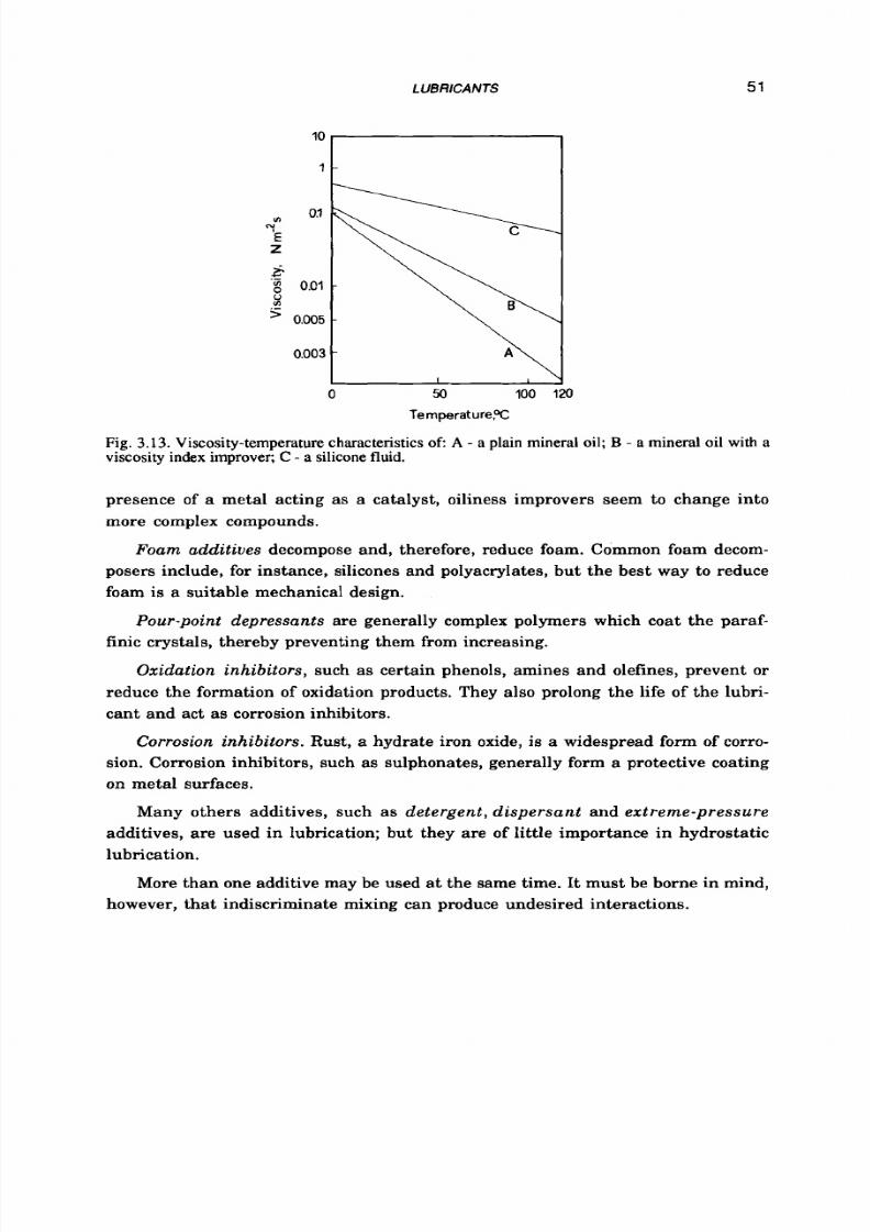
8/9/2019 Hydrostatic Lubrication 1992
http://slidepdf.com/reader/full/hydrostatic-lubrication-1992 68/558
LUBRICANTS
5 1
10
1 -
.-
In
0.003
0 50
100
120
I
.-
In
0.003
0 50
100
120
Temperature,%
Fig. 3.13. Viscosity-temperature characteristics o f A -
a
plain mineral oil;
B -
a mineral oil with a
viscosity index improver; C - a silicone fluid.
presence of a metal acting as a catalyst, oiliness improvers seem to change into
more complex compounds.
Foam additives
decompose and, therefore, reduce foam. Common foam decom-
posers include, for instance, silicones and polyacrylates, but the best way to reduce
foam is
a
suitable mechanical design.
Pour-point depressants are generally complex polymers which coat the paraf-
finic crystals, thereby preventing them from increasing.
Oxidation inhibitors, such as certain phenols, amines and olefines, prevent o r
reduce the formation of oxidation products. They also prolong the life of the lubri-
cant and act as corrosion inhibitors.
Corrosion inhibitors.
Rust, a hydrate iron oxide,
is
a widespread form of corro-
sion. Corrosion inhibitors, such as sulphonates, generally form a protective coating
on metal surfaces.
Many others additives, such as de te rgen t, d i spe rsan t and ex treme-pre ssure
additives, are used in lubrication; but they are of little importance in hydrostatic
lubrication.
More than one additive may be used a t the same time. It must be borne in mind,
however, that indiscriminate mixing can produce undesired interactions.

8/9/2019 Hydrostatic Lubrication 1992
http://slidepdf.com/reader/full/hydrostatic-lubrication-1992 69/558
5 2 HYDROSTATIC LUBRlCATlON
3.3 SYNTHETIC LUBRICANTS
The performance of synthetic lubricants is better than that of mineral lubri-
cants, but the former are much more expensive. They are often used in extreme
conditions, for instance in cases of high pressure or temperature.
Synthetic lubricants include the following:
Synthetic hydrocarbons; the polyolefins and hydrobenzene in particular,
Organic esters; those of dibasic acids in particular, which also have very good
Phosphatic esters, whose oiliness is very good and whose thermal stability is
Polyglicols,
with very good oiliness, a high VZ and also fluidity a t low temper-
atures.
Silicones (with a polymer-like structure, in which the carbon is replaced by
silicon). They have a high VZ (see a lso Fig. 3.131, a high flash-point, a low pour-
point, high thermal stability and oxidation stability and a good anti-foam perfor-
mance. On the other hand, their oiliness is poor.
which have very good fluidity a t low temperatures, and a very good VZ.
fluidity a t low temperatures, and good thermal stability.
fair.
Various synthetic lubricants may be used
as
additives.
On lubricants see also ref. 3.11.
REFERENCES
3.1
39
3.3
3.4
3.6
3.6
3.7
Dorinson A., Ludema
K.
C.; Mechanics and Chem istry in Lubrication ; Else-
vier, Amsterdam, 1985; 634 pp.
O'Connor
J.,
Boyd
J.;
Standard Handbook
of
Lubrication Engineering; Mc
Graw-Hill, New York, 1968.
Wills J. G.; Lubrication Fundamentals; M. Dekker Inc., New York, 1980; 465
PP.
Booser E.
R.;
Handbook
of
Lubrication, 2nd
Vol. ; CRS
Press, Boca Raton
(Florida), 1984; 689 pp.
McCloy D., Martin H. R.; Control of Fluid Power; Ellis Horwood Ltd., Chich-
ester, 1980;505 pp.
Liste des Caractkristiques Exigkes pour les Fluides Olkohydrauliques; CETOP
(ComitB Europben des Transmissions Olbohydrauliques et Pneumatiques),
London, 1971.
Fowle T;
Aeration in Lubricating Oils;
Tribology International,
14
(19811, 151-
157.

8/9/2019 Hydrostatic Lubrication 1992
http://slidepdf.com/reader/full/hydrostatic-lubrication-1992 70/558
LUBRICANTS
53
3.8 Raznyevich K.;
ables et Diagrammes Thermodynamiques;
Eyrolles, Didion,
1970.
3.9
Speich
H.,
Bucciarelli
A.;
L’Oteodinamica; Techniche nuove, 1971; 727 pp.
3.10 Neale
J.
M.; ribology Handbook;
Butterworths, London, 1973.
3.11 Lansdown
A. R.;
Lubrication. A Practical Guide to Lubricant Selection;
Pergamon Press, Oxford, 1982; 252 pp.
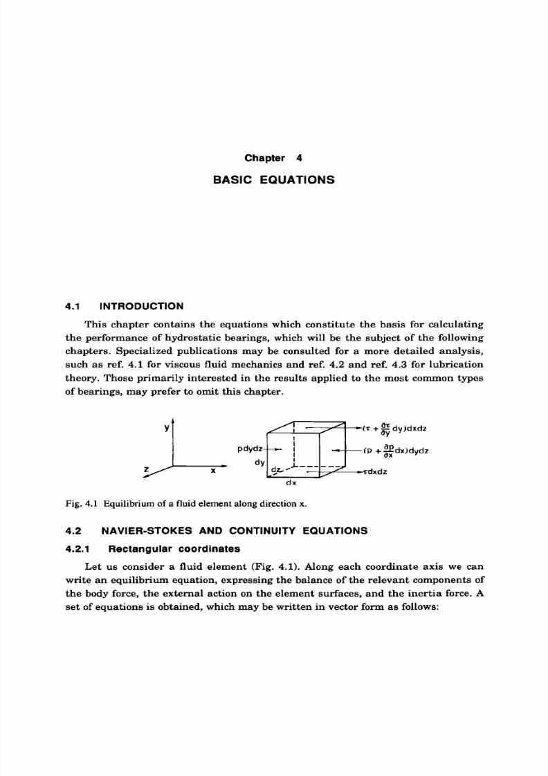
8/9/2019 Hydrostatic Lubrication 1992
http://slidepdf.com/reader/full/hydrostatic-lubrication-1992 71/558
Chapter 4
BASIC
EQUATIONS
4.1 INTRODUCTION
This chapter contains the equations which constitute the basis for calculating
the performance of hydrostatic bearings, which will be the subject of the following
chapters. Specialized publications may be consulted for a more detailed analysis,
such a s ref.
4.1
or viscous fluid mechanics and ref.
4.2
nd ref. 4.3
or
lubrication
theory. Those primarily interested in the results applied to the most common types
of bearings, may prefer to omit this chapter.
d x
Fig.
4.1
Equilibrium
of
a fluid element along direction x.
4.2 NA VIER-STOK ES AND CONTINUITY EQUA TIONS
4.2.1 Rectan gu lar co ord inates
Let us consider a fluid element (Fig. 4.1).Along each coordinate axis we can
write an equilibrium equation, expressing the balance of the relevant components of
the body force, the external action on the element surfaces, and the inertia force. A
set of equations is obtained, which may be written in vector form as follows:

8/9/2019 Hydrostatic Lubrication 1992
http://slidepdf.com/reader/full/hydrostatic-lubrication-1992 72/558
BASlC
EQUATlONS
55
(4.1)
v
p E = p f + V o
In the preceding statement (generally called the momentum equation),
f
is the body
force per unit mass, V o is the divergence of the stress tensor, v
is
the velocity vector.
D/Dt means the total (also called "material") time derivative:
In order to reduce the number of unknowns, one must resort to the constitutive
equations of the medium. Here we shall consider isotropic fluids alone, with a lin-
ear relationship between stresses and strain rates (Stokes law of friction) and with
no bulk viscosity (Stokes approximation). On these assumptions, the constitutive
equations may be written in the following form:
The tensors
I
and Dq are the unit tensor and the so-called strain rate deviator
respectively. With these equations, we have implicitly defined "pressure" p as the
opposite
of
the mean principal stress and "viscosity"
p
as the coefficient of propor-
tionality between the shearing stresses and the shearing strain rates ( S i j is the
well-known Kroneker delta).
The "Navier-Stokes" equations are obtained by combining Eqn 4.1 nd Eqn 4.2:
where
u,
u, w and
X, ,
Z are the components of the velocity vector and of the body
force (per unit mass), respectively.
Since four unknowns are involved (namely, the velocity components and the
pressure), another equation is needed: this is the "continuity" equation, expressing
the balance of the mass flowing through an infinitesimal control volume:
(4.4)
a a a
ay
+
(PU) +
-
pv)+ (pw)=
0
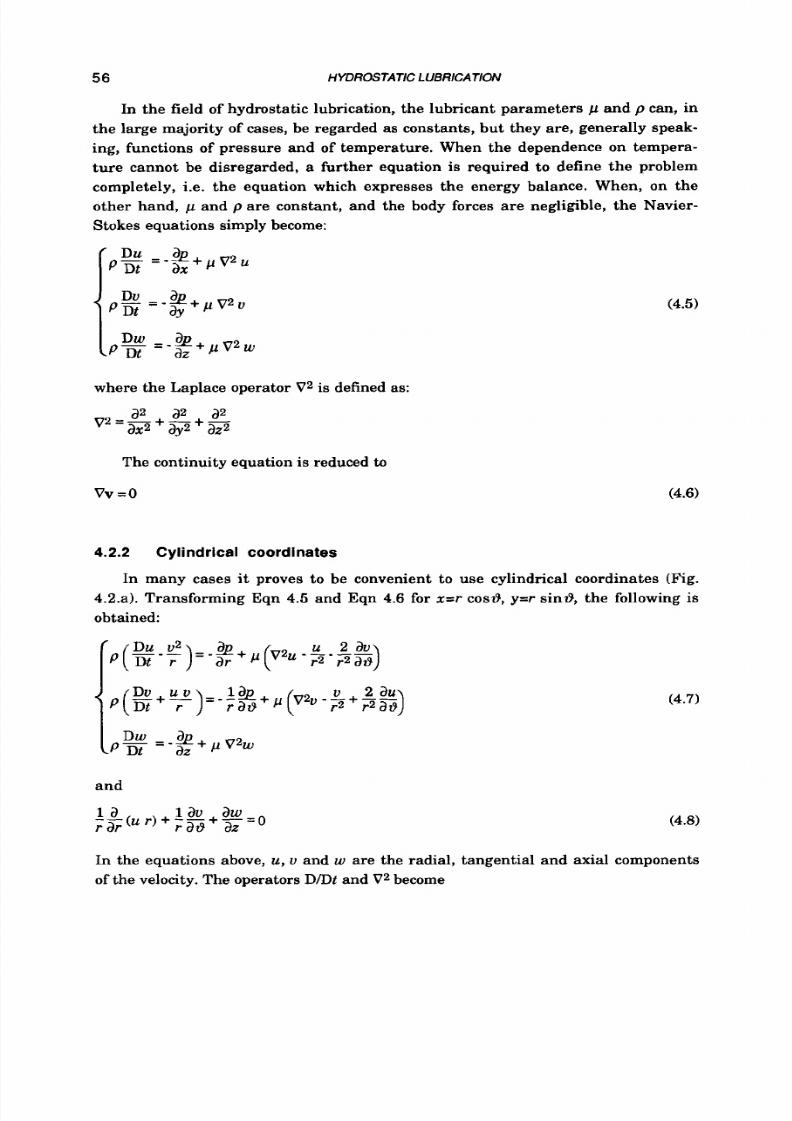
8/9/2019 Hydrostatic Lubrication 1992
http://slidepdf.com/reader/full/hydrostatic-lubrication-1992 73/558
5 6
HYDROSTATICLUBRICATION
In the field of hydrostatic lubrication, the lubricant parameters
p
and p can, in
the large majority of cases, be regarded as constants, but they are, generally speak-
ing, functions of pressure and of temperature. When the dependence on tempera-
ture cannot be disregarded,
a
further equation is required
t o
define the problem
completely, i.e. the equation which expresses the energy balance. When, on the
other hand,
p
and p are constant, and the body forces are negligible, the Navier-
Stokes equations simply become:
where the Laplace operator V 2 is defined as:
The continuity equation is reduced to
vv
=o
(4.6)
4.2.2 Cylindrical coordinates
In many cases it proves to be convenient to use cylindrical coordinates (Fig.
4.2.a). Transforming Eqn 4.5 and Eqn 4.6 for
z=r
COSB, =r sin6 , the following is
obtained:
and
(4.7)
(4.8)
In
the equations above, u , u and
w
are the radial, tangential and axial components
of the velocity. The operators
DDt
and V 2 become
8/9/2019 Hydrostatic Lubrication 1992
http://slidepdf.com/reader/full/hydrostatic-lubrication-1992 74/558
BASIC EQUATIONS
57
~a a v a a
~t
at
ar rat9 az
-++-+--+w-
- b -
Fig. 4.2 Coordinate systems:a- cylindrical coordinates; b- spherical coordinates.
4.2.3 Spherical coordinates
y=r si nq sinI9,
z=r
cosq) the Navier-Stokes an d continuity equations become:
In the spherical coordinate system
of
Fig. 4.2.b (i.e.:
x = r
s i n q cos19,
(4.9)
and
1
aw
v sinq)
+--
=
2 U
r2)
+
--
r
sinq
at9
_ _a
i a
r
sinq
329
where
(4.10)

8/9/2019 Hydrostatic Lubrication 1992
http://slidepdf.com/reader/full/hydrostatic-lubrication-1992 75/558
58 HYDROSTATIC LUBRICATION
The symbols
u ,
u , and w now indicate the components of the fluid velocity in the r , Q
and
0
directions, respectively.
4.3
THE REYNOLDS EQUA TION
4.3.1 Rectangular coordinates
In the field of fluid film lubrication we are involved in most cases with the study
of thin films (Fig. 4.3). n this connection, the complexity of the Navier-Stokes equa-
tions may be greatly reduced, thanks to the following considerations:
-
he thickness
of
the fluid film (in the
y
direction, in Fig.
4.3)
s small, compared to
it s size in the other directions;
-
consequently, the pressure, as well as the density and the viscosity, may be aver-
aged alongy: i.e. it
is
stated that
aplay=O,
rlay=O, apJay=O;
- compared to aulay and
awldy
all the other velocity gradients are negligible; this is
justified because u and
w
are generally much greater than u , and the film thickness
along y is small;
- he flow is laminar: no turbulence nor vortex exists;
- he body forces are negligible compared to the viscous forces;
-
he inertia terms, too, are negligible compared to the viscous forces, i.e.
Du/Dt=Du/Dt=Dw/Dt=O;
-
on the surfaces bounding the fluid film, the velocity
of
the lubricant coincides with
the velocity of the surfaces.
Accepting the foregoing assumptions, the second of Eqns 4.3 can be released,
while the others become:
t
2
/-
Fig. 4.3 Thin fluid film.
8/9/2019 Hydrostatic Lubrication 1992
http://slidepdf.com/reader/full/hydrostatic-lubrication-1992 76/558
BASIC EOUATlONS
59
az
14.11)
The first of Eqns 4.11 may now be integrated twice, with the boundary conditions
u=U1for y=O and u=U2
for
y=h, to obtain the component of the fluid velocity in the
x
direction:
u = L*yDax 0,
-
h)+
(1
- f Ul + f U2
In the same way the component
(4.12)
(4.13)
is found, from the second of Eqns 4.11, with the boundary conditions
w=O
for y=O and
y = h (in other words, we have assumed that the surfaces of the pair do not slide in
the z direction).
Let us now integrate the continuity equation (Eqn 4.4) along the thickness of the
fluid film:
h
h h
h
Substituting the above expressions for u and w and using V=u(h)-v(0)o indicate the
squeeze velocity of the surfaces, it is easy to find:
$(?$) +
$(?$) = 6 [ p h (U1+U2)]
12
p U 2 zh + 12 p
V +
2 h
(4.14)
Equation 4.14 is the generalized Reynolds equation, which is characteristic of
hydrodynamic lubrication (see also
ref.
4.4).
Concerning plane hydrostatic bearings, velocities
U1
and
U2
of the surfaces
often do not depend on the coordinates; furthermore,
it
is generally assumed that
the density and the viscosity of the lubricant do not appreciably vary in the film.
Since velocity
V
may be written a s
equation 4.14 is simplified t o
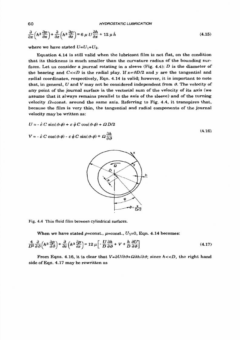
8/9/2019 Hydrostatic Lubrication 1992
http://slidepdf.com/reader/full/hydrostatic-lubrication-1992 77/558
6 0 HYDROSTATIC LUBRICATlON
(4.15)
where we have stated U=Ul+U2.
Equation 4.14 is still valid when the lubricant film is not flat, on the condition
that
its
thickness
is
much smaller than the curvature radius of the bounding sur-
faces. Let us consider a journal rotating in a sleeve (Fig. 4.4): D is the diameter
of
the bearing and C c c D
is
the radial play. If x=6D/2 and
y
are the tangential and
radial coordinates, respectively, Eqn. 4.14 is valid; however,
it
is important
to
note
that, in general,
U
and
V
may not be considered independent from
6.
The velocity of
any point
of
the journal surface is the vectorial sum
of
the velocity of its axis (we
assume that i t always remains parallel to the axis
of
the sleeve) and of the turning
velocity R=const. around the same axis. Referring
to
Fig.
4.4,
it transpires that,
because the film is very thin, the tangential and radial components of the journal
velocity may be written as:
Fig. 4.4 Thin fluid film between cylindrical surfaces.
When we have stated p=const., p=const.,
U1=0,
qn. 4.14 becomes:
(4.16)
(4.17)
From Eqns.
4.16,
it
is
clear that V=dUla&&?ahlals;ince h<cD, the right hand
side of Eqn.
4.17
may be rewritten as
8/9/2019 Hydrostatic Lubrication 1992
http://slidepdf.com/reader/full/hydrostatic-lubrication-1992 78/558
BASIC EQUATIONS
61
After having substituted Eqns 4.16 and the film thickness:
h
=
C
[l-
COS(~$)] ;
we finally obtain
In the last equation, the term proportional to sin2(6-@)may also be disregarded,
since, on average, it is much smaller than the others.
4.3.2
Cylindrical coordinates
Let us consider a thin plane clearance: when we state the usual simplificative
hypotheses above, the Navier-Stokes equations (Eqns 4.7), are reduced to the
following:
(4.19)
In the first equation the inertia term pv2/r has been retained, since it may prove not
to be negligible
at
high turning velocity, as will be shown in sect. 6.2.1.
Integrating the second of Eqns 4.19, with the boundary conditions
v(O)=O,
v(h)=V,
he tangential velocity of the fluid is obtained:
(4.20)
Substituting it in the &st of Eqns 4.19 and integrating for u(O)=O,
u(h)=U,
he radial
velocity turns out to be (after further simplification):
(4.21)
Let us now integrate the continuity equation (Eqn
4.8)
along the film thickness:
8/9/2019 Hydrostatic Lubrication 1992
http://slidepdf.com/reader/full/hydrostatic-lubrication-1992 79/558
6 2
h
HYDROSTATIC LUBRICATION
Substituting in it Eqn
4.20
and Eqn
4.21,
the Reynolds equation i s obtained:
+ 1 2 p W + ~ ; z ( h 3 V 2 )~ 3 (4.22)
where
W=h=w(h)-w(O)
s the squeezing velocity of the surfaces.
If the upper surface does not slide, but rotates around the z axis
at
a constant
speed
0,
t is
U=O
nd V=r; Eqn 4.22 now becomes:
Equation 4.22 may also be used for a conical film, provided the thickness of the
film is much smaller than the minimum curvature radius, i.e. all the points of the
domain are far enough from the vertex
of
the cone.
With reference to the coordinate system
in
Fig. 4.5, Eqn 4.22 may be rewritten
as:
If we now assume that the axes of the conical surfaces bounding the lubricant
film always remain parallel (i.e. the thickness of the film does not depend on r) ,and
that the turning velocity of the journal is Ckconst., it is possible to obtain simple
expressions for U, , W. The velocity of each point of the surface of the journal is the
vectorial sum of the velocity of its axis, plus the turning velocity around the same
axis; hence, the velocity components are:
u E c sina cos(++) + E c sina sin(+@) R g a s V, cosa
ah
V =
E
C sin(+@
+
E ~ Cos(+$) +
0 r
ina
w = -
E
C cosa cos(99) - E C cosa sin(+$) + O x V , sina
(4.25)
ah,
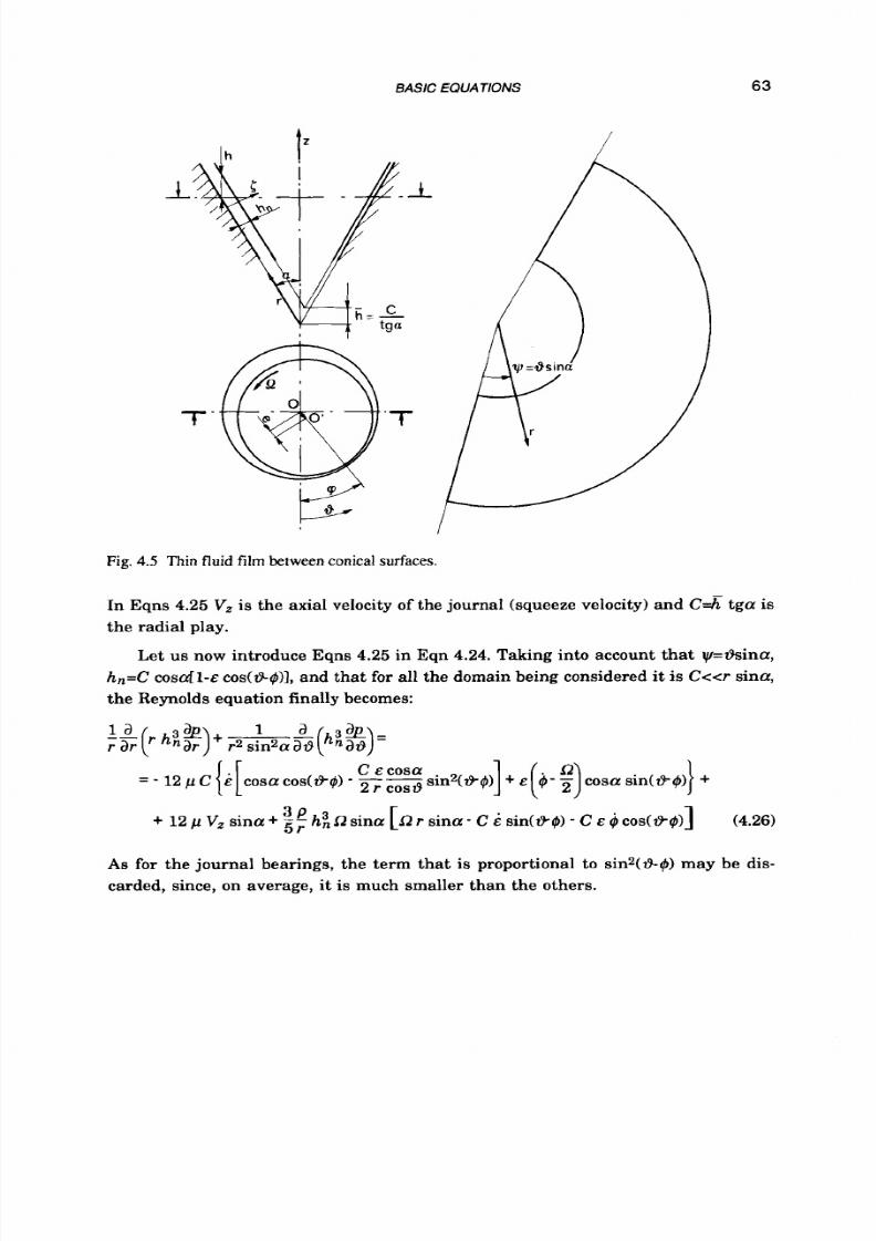
8/9/2019 Hydrostatic Lubrication 1992
http://slidepdf.com/reader/full/hydrostatic-lubrication-1992 80/558
BASIC EQUATIONS
63
Fig.
4.5 Thin
fluid
film between conical surfaces.
In Eqns 4.25V,
is
the axial velocity
of
the journal (squeeze velocity) and
C&
tga is
the radial play.
Let
us
now introduce Eqns
4.25
n Eqn
4.24.
Taking into account tha t yl=&ina,
hn=C cosafl-e cos(&$)], and that for all the domain being considered it is C<<r sina,
the Reynolds equation finally becomes:
+ 12
p V, sina + 3 P; hnlZ sina [lZ r sina - C
&
sin(+@)
C
E 4 cos(+$)]
(4.26)
A s
for the journal bearings, the term that is proportional to sins(&-$)may be dis-
carded, since, on average, i t is much smaller than the others.
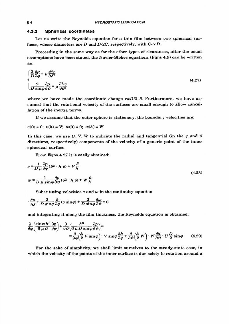
8/9/2019 Hydrostatic Lubrication 1992
http://slidepdf.com/reader/full/hydrostatic-lubrication-1992 81/558
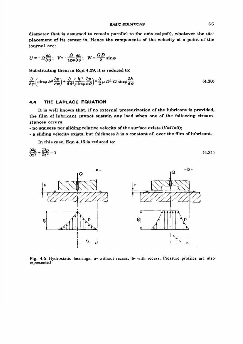
8/9/2019 Hydrostatic Lubrication 1992
http://slidepdf.com/reader/full/hydrostatic-lubrication-1992 82/558
BASIC EQUATIONS 65
diameter that
is
assumed
to
remain parallel to the axis
z=(p=O),
whatever the dis-
placement of its center is. Hence the components of the velocity of
a
point of the
journal are:
Substituting them in Eqn 4.29,
it is
reduced to:
(4.30)
4.4 THE LAPLACE EQUATION
It is well known that, if no external pressurization of the lubricant
is
provided,
the film of lubricant cannot sustain any load when one of the following circum-
stances occurs:
-
no squeeze nor sliding relative velocity of the surface exists
(V=U=O);
-
a sliding velocity exists, but thickness h
is
a constant all over the film of lubricant.
In this case, Eqn
4.15 is
reduced
to:
- a - -
- b -
(4.31)
Fig. 4.6 Hydrostatic bearings: a- without recess; b- with recess. Pressure profiles are also
represented
8/9/2019 Hydrostatic Lubrication 1992
http://slidepdf.com/reader/full/hydrostatic-lubrication-1992 83/558
6 6
HYDROSTATIC LUBRICATION
which is the so-called Laplace equation, for which, as is well known, only one
solu-
tion exists when the value of p on the boundary is assigned. Furthermore, if p is a
constant on the entire boundary (e.g. the atmospheric pressure), it takes on the
same value on all the inner points as well.
So,
if the boundary pressure i s the atmo-
spheric pressure, a source of pressurized lubricant must be provided to ensure a
lubricant film between the surfaces, as in Fig. 4.6.a; this is precisely the principle of
hydrostatic lubrication. In Fig. 4.6.b a recess is widened around the source, in
which the pressure is constant. Of course, both the hydrostatic and the hydrody-
namic pressure fields may exist at the same time, as in the so-called
"hybrid"
bearings.
4.5
4.5.1 Lo ad capacit y
LOAD CAPACITY, FLOW RATE, FRICTION
The load capacity W of a film of lubricant is defined as the resultant of the pres-
sure field. Hence, if A is the surface on which the pressure acts, and n s its normal
direction. it is:
4.5.2
Flow
rate
Integrating the velocity components (Eqn 4.12 and Eqn 4.13) between y=O and
y=h,
the components of the flow rate per unit length q are obtained:
(4.32)
(it should be borne in mind that Eqn 4.12 and Eqn 4.13, and consequently Eqns 4.32,
refer
t o
the case of two planes sliding one on the other in the
x
direction).
For a system of polar coordinates, Eqns 4.32 are best substituted by the following:
(4.33)
where it has been assumed that the upper surface
(z=h)
of the pair rotates around
the z axis.

8/9/2019 Hydrostatic Lubrication 1992
http://slidepdf.com/reader/full/hydrostatic-lubrication-1992 84/558
BASIC
EQUATIONS
67
To obtain the volume
flow
rate of lubricant crossing a certain contour S, whose
external normal direction is n, t is necessary to integrate the scalar product qn:
Q =
q.n
dS
S
4.5.3 Frict ion
In connection with bearings, it is important to evaluate the friction forces on the
surfaces.
The shearing stresses in the lubricant can be found by means
of
the constitutive
equations (Eqn
4.2).
On the basis of the assumptions stated in section
4.3,
they are
reduced to:
i.e. t o the well-known Newton formula of the shear stress (see also sect. 3.2). Substi-
tuting Eqn 4.12 and Eqn 4.13 in these equations, we obtain:
(4.34)
When the pressure field is known, (that is after the relevant Reynolds equation
has been solved), Eqns 4.34 directly give the shearing stresses in the film of lubri-
cant between two surfaces sliding with a relative velocity U=U2-U1 in the x direc-
tion. The stresses on the surface
y=O are, therefore,
On the opposite surface
( y = h )
we have:
8/9/2019 Hydrostatic Lubrication 1992
http://slidepdf.com/reader/full/hydrostatic-lubrication-1992 85/558
6 8 HYDROSTATIC LUBRICATION
Integrating shear stress
z,
one obtains the tangential force on the surfaces.
Hence in the direction of the sliding velocity, the total drag is:
(4.35)
the upper sign referring to the fixed surface
(y=O),
the lower to the moving surface
( y = h ) .
In
a
very similar way, it
is
possible t o evaluate the friction moment which acts
on two surfaces rotating around a common axis, with a relative velocity
Lk
(4.36)
4.6
THE ENERGY EQUATION
A s has been already pointed out, the characteristics of a fluid depend on tem-
perature T. n particular, for the most common lubricants, the variation in viscos-
ity is notable, even for temperature changes of few degrees. Thus, in order to carry
out a rigorous analysis, ,u should be considered as a function of the temperature,
and a new equation is required to compensate for the introduction of the new
unknown.
The energy equation i s obtained by imposing the energy balance for an infinites-
imal control volume. Assuming that heat radiation
is
negligible and tha t no heat is
generated in the fluid (except for the dissipation of mechanical work due to shear-
ing), we obtain (ref.
4.2):
(4.37)
In the equation above, the left-hand side is the rate of change in internal energy of
the fluid (c being its specific heat). On the right-hand side, the first term accounts
for the power due t o the expansion in volume of the fluid; the second term accounts
for the heat conduction in the fluid
(k
being the coefficient of thermal conductivity);
the last term is the dissipation of mechanical power.
Since the energy equation must be applied
t o
the thin films typical of hydrostatic
and hydrodynamic lubrication, some further simplification can be introduced:
-
he specific heat
is
a constant (since no great temperature change
is
expected),
as
well
as
coefficient k;

8/9/2019 Hydrostatic Lubrication 1992
http://slidepdf.com/reader/full/hydrostatic-lubrication-1992 86/558
BASIC EQUATIONS
69
-the fluid is considered
to
be incompressible (hence Eqn 4.6
is
valid);
-only steady-state conditions are considered (i.e.
aT/dt=O).
Introducing Eqn 4.2 in Eqn 4.37, we obtain:
A s in section 4.3, it is possible to disregard all the velocity gradients, except for au&
and awlay . Furthermore, heat conduction in the x and z direction is small, com-
pared to the convective term; thus Eqn 4.38 becomes:
(4.39)
Heat conduction may sometimes be totally disregarded (i.e. k=O) as well as the
heat transfer to the boundaries (adiabatic flow).
A similar equation may be obtained in cylindrical coordinates. Limiting our-
selves to axial-symmetric configurations, we find:
(4.40)
4.7 LAMINAR FLOW THROUGH CHARACTERISTIC CONFIGURATIONS
4.7.1 Parallel surfaces
Let us consider a plane surface of infinite length moving on another with veloc-
ity U Fig. 4.7.a).
The velocity of the lubricant is obtained from Eqn 4.12:
(4.41)
When
U=O,
the velocity profile is a parabola, whose axis of symmetry is y = h / 2
(pressure flow, or "Poiseuille
flow").
In general, the linear term
Uy
/ h (shear flow
o r
"Couette flow") has to be added
t o
the parabola. In Fig. 4.7.b the velocity profile is
plotted for certain values of the non-dimensional pressure gradient
P* =& (-g)
When p*<O, the two terms on the right-hand side of Eqn 4.41 are opposite in sign,
and when p*<-1 an inversion of the flow occurs. The lat ter condition is determined
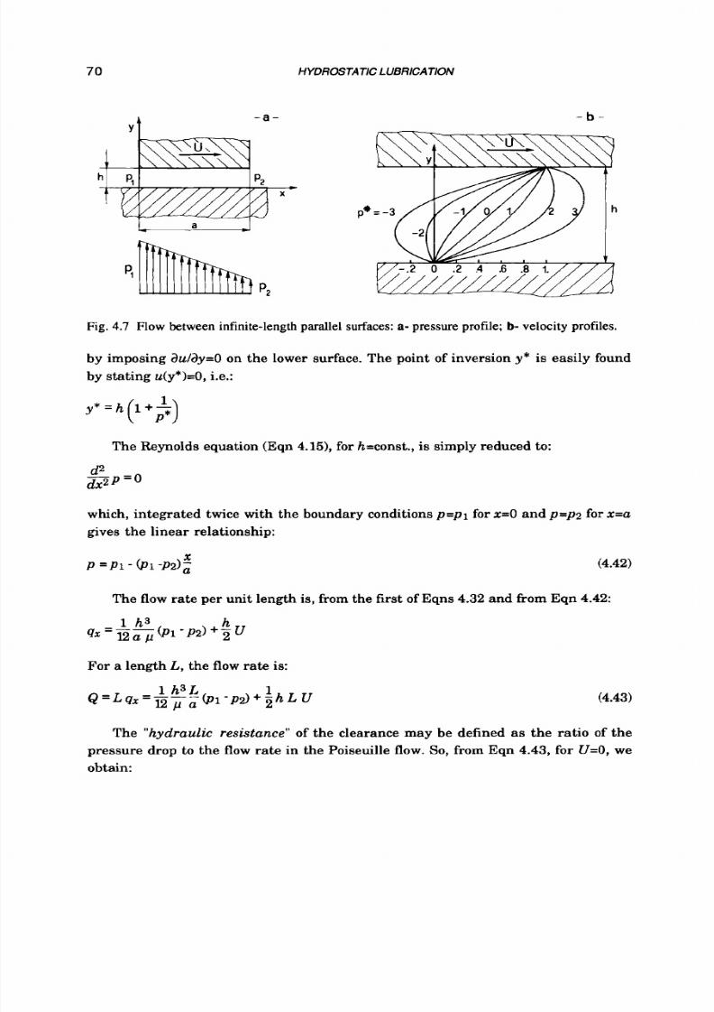
8/9/2019 Hydrostatic Lubrication 1992
http://slidepdf.com/reader/full/hydrostatic-lubrication-1992 87/558
70
- a -
Y t
HYDROSTATICLUBRICATlON
- b -
L a
J
Fig. 4.7 Flow between infinite-length parallel surfaces: a- pressure profile;
b-
velocity profiles.
by imposing aufay=O on the lower surface. The point of inversion y*
is
easily found
by stating u(y*)=O, i.e.:
The Reynolds equation (Eqn 4.15), for h=const.,
is
simply reduced to:
which, integrated twice with the boundary conditions p = p 1 for
x=O
and p = p 2 for x=a
gives the l inear relationship:
(4.42)
P =P 1 -
@ 1 -P2) ,
The flow rate per unit length
is,
from the
first
of Eqns
4.32
and
from
Eqn
4.42:
For a length L, the
flow
rate is:
The "hydraulic
resistance"
of the clearance may be defined as the ratio of the
pressure drop to the flow rate in the Poiseuille flow.
So,
from Eqn
4.43,
for
U=O,
we
obtain:

8/9/2019 Hydrostatic Lubrication 1992
http://slidepdf.com/reader/full/hydrostatic-lubrication-1992 88/558
BASIC
EQUATIONS
71
(4.44)
The tangential force on the moving surface is given by Eqn
4.35:
It should be stressed that, in order that
flow
is laminar as presumed, Reynolds
number
R e Z P u h (4.45)
P
should be lower than the critical value
Re=2300.
In
Eqn
4.45
u
s the mean velocity
4.7.2
Infinite-length rectangular
pad.
Let us consider a segment
L
of a hydrostatic pad of infinite length, as in Fig.
4.8.
The recess is bounded by
two
clearances. If we now use
p
t o indicate the relative
pressure in the clearances, and
p r t o
indicate the relative recess pressure (which
can be considered
to
be constant, since the recess depth is much greater than the
thickness of the film), from Eqn 4.42 we get:
(4.46)
The load capacity of the pad is found by integrating the pressure on the
two
land
areas and adding the contribution p r L b
of the recess:
~ r 2
The total
flow
of the pad is found from Eqn 4.43:
1 1 L
& = - -
h3
~ - b
r
3 P
The hydraulic resistance may therefore be defined as
(4.47)
(4.48)
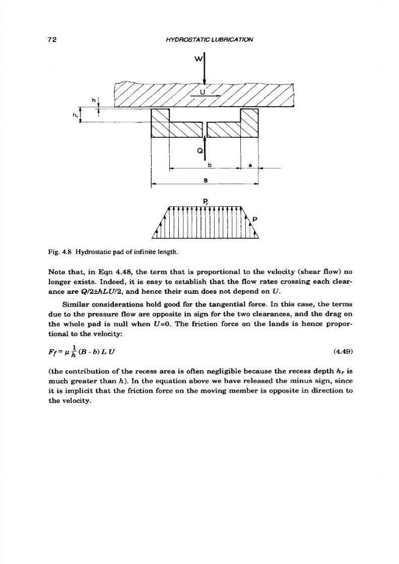
8/9/2019 Hydrostatic Lubrication 1992
http://slidepdf.com/reader/full/hydrostatic-lubrication-1992 89/558
72
HYDROSTATIC LUBRICATION
Fig.
4.8
Hydrostatic
pad
of infinite length.
Note that , in Eqn 4.48, the term tha t i s proportional to the velocity (shear flow) no
longer exists. Indeed, it is easy to establish that the flow rates crossing each clear-
ance are Ql 2UL Ul 2 , and hence their
s u m
does not depend on
U .
Similar
considerations hold good for the tangential force. In
this
case, the terms
due to the pressure flow are opposite in sign for the two clearances, and the drag on
the whole pad is null when U=O. The friction force on the lands is hence propor-
tional
to
the velocity:
(the contribution of the recess area is often negligible because the recess depth
h ,
is
much greater than h). In the equation above we have released the minus sign, since
it is implicit tha t the friction force on the moving member is opposite in direction to
the velocity.

8/9/2019 Hydrostatic Lubrication 1992
http://slidepdf.com/reader/full/hydrostatic-lubrication-1992 90/558

8/9/2019 Hydrostatic Lubrication 1992
http://slidepdf.com/reader/full/hydrostatic-lubrication-1992 91/558
74
HYDROSTATIC LUBRICATION
The friction force over the moving member is (Eqn 4.35)
FC, .= 4UA
IL
' h r
For a sliding hydrostatic pad this force should be added t o the friction force on the
lands, obtaining a total friction force
where A1 and
A,.
are the land and recess area, respectively, and factor
fr
takes on a
value
h
f , .=4-
h r
under the simplifying assumptions made above.
More detailed and thorough studies of recess flow recirculation can be found in
ref. 4.5. and ref. 4.6. Better approximations for critical velocity and recess friction
factor are to be found in ref. 4.6:
h h
f,.
= (4
- 3
- -
hr hr
(4.52)
(4.53)
All the foregoing equations are based on the assumption that recess flow is
laminar, i.e. that the Reynolds number
is
smaller than
1000.
Actually, the problem is more complex because of the pressure
head build-up a t the inlet of the clearance (ref. 4.7).
For turbulent flow it may be stated that:
f =--fe h
r 2 h , P
(4.54)
and
f,
may be read in Fig.
4.9.b
(proposed in ref. 4.5 on the basis of experiments on
journal bearings) or calculated (ref.
4.8)
from the equation
(4.55)

8/9/2019 Hydrostatic Lubrication 1992
http://slidepdf.com/reader/full/hydrostatic-lubrication-1992 92/558
BASIC
EQUATIONS
75
4.7.4 Annular clearance.
Let u s examine the flow between two parallel ring-shaped walls (Fig.4.101, o-
tating around the z-axis with a relative velocitya,which, however, is not
so
great as
to require the effects of the inertia of the lubricant t o be considered. Since the thick-
ness of the film is small, compared to width r2-r-1,Eqn
4.23
(the Reynolds equation)
is valid, which, due to the radial symmetry, is now reduced to
Integrating it twice, with the boundary conditions
p = p 1 at r = r l , p = p 2 at r = r 2 ,
the pressure field is obtained:
In rlr2
P
' P 2 +
( P 1
- P 2 ) & &
i.e. p decreases on the land area with a logarithmic trend.
The flow rate per unit length is, from the first of Eqns 4.33and Eqn
4.57,
(4.56)
(4.57)
Fig.
4.10
Annu lar clearance.

8/9/2019 Hydrostatic Lubrication 1992
http://slidepdf.com/reader/full/hydrostatic-lubrication-1992 93/558
76
HYDROSTATIC LUBRICATION
Consequently, the total flow across any circle
of
radius
r1esr-2
is
(4.58)
Hence, the “hydraulic resistance“ of the clearance may be defined
as:
(4.59)
P 1 - p 2 =6
In
r 2 h
Q n p 7
The friction moment, from Eqn 4.36, is:
The Reynolds number is again given by Eqn 4.45. Since the mean velocity at
mean radius
7=(rl+r2)/2
s
8
-
.
2 x F h ’
it follows that:
1 P 1
R e = - - Q
” 2 ( 1 + 3
(4.61)
4.7.5
Circular pad
The simple hydrostatic bearing, shown in outline in Fig.
4.6.b, is
made up of a
circular recess bounded by an annular clearance, like the one examined
in
the
previous section. Assuming that
p 2 = 0
(ambient pressure), pressure
p r
in the recess
is related to the ra te of
flow by Eqn
4.58,
which can be rewritten as
The pressure in the clearance decreases with a logarithmic trend,
(4.62)
given by Eqn
4.57,
in which
p l=pr
and
p2=0.
The hydraulic resistance i s still given by Eqn
4.59.
The load capacity of the pad is found by integrating the pressure on the land
area and adding the term
m$pr
due to the recess pressure:
(4.63)

8/9/2019 Hydrostatic Lubrication 1992
http://slidepdf.com/reader/full/hydrostatic-lubrication-1992 94/558
BASIC
EQUATIONS
If Eqn
4.62
is introduced in Eqn
4.63,
we obtain
W = 3 - Q$ ( - - )
77
(4.64)
The friction moment is given by Eqn 4.60, since the friction in the recess is
negligible.
4.7.6 Pipes
In the case of laminar flow in a straight circular pipe, whose length
is
much
greater than the diameter, certain simplifying hypotheses,
similar to
those stated in
section
4.3,
may be applied
t o
the Navier-Stokes equations. In particular, the pres-
sure can be considered t o vary with the z coordinate alone. The third
of
Eqns 4.7 is
now reduced t o the following:
Integrating it with the boundary conditions w=O for r=d/2 and aw/&=o for r=O (due
to matters of symmetry), the velocity field
is
obtained as a function of the pressure
gradient:
(4.65)
which is the equation of a paraboloid. The maximum velocity of the fluid is at
r=O:
while
its
mean velocity
is:
Since the continuity equation (Eqn 4.8)
is
reduced t o dpldz=const., the pressure drop
along the pipe is linear. If a length 1 is considered, the flow rate is related t o the
pressure drop by the law:
Equation
4.66
is used
to
evaluate the hydraulic resistance:
(4.66)
(4.67)

8/9/2019 Hydrostatic Lubrication 1992
http://slidepdf.com/reader/full/hydrostatic-lubrication-1992 95/558

8/9/2019 Hydrostatic Lubrication 1992
http://slidepdf.com/reader/full/hydrostatic-lubrication-1992 96/558
BASIC
EQUATIONS 79
4.8
FLOW
INTO THE INLET LENGTH
inlet lengthIn section 4.7, a number
of
cases of laminar flow have been
examined; the equations which have been obtained expressing the flow as a
function of the pressure step are not strictly accurate, since certain distributed
energy losses have been disregarded. A s an example, let us consider a circular
pipe. When the fluid begins t o flow into the pipe, the velocity w is a constant for the
entire section (Fig. 4.12); the velocity of the fluid on the wall of the pipe, however, is
null, and this layer exerts a great shearing stress on the inner layers, whose
velocity must become greater than the mean value
W
in order to satisfy the
continuity requirement. The thickness
of
the
"boundary layer"
grows until, a t a
distance l i from the inlet, the whole section of the pipe is involved; a t this point, the
fluid velocity reaches the parabolic profile already seen in sect.4.7.6, and remains
so
thereafter.
\
-
'.
,
I
I
I
I
I
I
1 2
Fig. 4.12 Velocity profiles in the inlet length of pipes.
The length
Zi
is named
"inlet length"
(ref. 4.9) and its value is found to be
li=0.0575
d
Re.
When the length of the pipe is greater than
li,
which
is
generally true
for the capillaries used as compensating devices for hydrostatic bearings, Eqn 4.65
should be substituted by the following:
(4.69)
1 1
128
'
d 1
= - - d 4
1+0.0356i
Re
In other words, the value of the flow rate found in sect. 4.7.6 should be multiplied for
a correction coefficient, which accounts for the pressure loss required to accelerate
the inner fluid layers in the inlet length.

8/9/2019 Hydrostatic Lubrication 1992
http://slidepdf.com/reader/full/hydrostatic-lubrication-1992 97/558
8 0
HYDROSTATIC LU5RlCATlON
Similar
considerations hoId good for pipes of different shapes,
and
for the clear-
ances of hydrostatic pads (see,
for
example, sect. 6.2.14~)).
4.9 INLET LOSSES
In the preceding section, the pressure loss in the inlet length of a circular pipe
was examined; other pressure losses occur in the tank near the pipe inlet and a t the
inlet itself.
The loss in the
tank
may be considered to be the sum of two terms: the first is
used
to
accelerate the fluid in the tank (in the conoid bounded by dotted lines in Fig.
4.12) to the inlet velocity, the other is due to the viscous dissipation in the same area.
The loss
at
the inlet, on the other hand, is due to the
"uenacontructu",
which
is
generally present, especially when the inlet edge is sharp.
The overall pressure loss is (ref 2.7):
(4.70)
The values of resistance coefficient k are given in Fig. 4.13 for the cases of (a) a
well-rounded entrance, (b) a slightly rounded entrance, (c) a sharp-edged entrance.
The pressure loss a t the inlet, given by Eqn 4.70, should be added to the pressure
loss in the pipe, given by Eqn 4.69.
- a - - b -
- C -
-
K
= 0.05
Fig. 4.13 Resistance coefficients
due to
the geometry
of
pipe entrances.
4.10 TURBULENT
FLOW
The flow of the lubricant in the gap between two close surfaces is , in most cases,
of a laminar kind, i.e. the Reynolds number is lower than 1000. Nevertheless, in
certain circumstances,
it
may be not so. For instance, with reference to
a
circular
pad and to Eqn
4.61,
if high values are selected for p r and
r h
due to the need to
sustain a heavy load) and if the viscosity of the lubricant
is
low (e.g. when water or

8/9/2019 Hydrostatic Lubrication 1992
http://slidepdf.com/reader/full/hydrostatic-lubrication-1992 98/558
BASIC EQUATIONS
81
liquid metals such as Sodium have to be used), and, above all, if the gap is higher
than the values commonly adopted, Re may be greater than 1000.
When
Re is
greater than
1000,
a transition regime sets in; a t
Rez2300
the flow is
prevalently turbulent, and it is totally turbulent for higher Reynolds numbers (see
ref. 4.10). When the fluid gets into the clearance, the boundary layer is at first lami-
nar but becomes turbulent (except for a thin laminar sublayer) at
a
distance from
the inlet of 25+40 times the clearance. The velocity profile is similar to the one plot-
ted in Fig. 4.14.b and the maximum fluid velocity is about 1.2 times it s mean value.
- a
-
- b -
Fig.
4.14
Velocity distribution in
a
pipe: a- laminar f l ow; b- turbulent f l o w .
In turbulent flow, the velocity components and the pressure in the clearance a t
a given time may be written as a sum of t w o terms:
u=u*+u1;
u=u*+u1; w=w*+wl;
p=p*+pl: the first terms are the average values, the others ar e the fluctuations due
to turbulence. These expressions should be introduced into Eqns
4.7
and Eqn
4.8
(i.e.
the Navier-Stokes and continuity equations). Certain assumptions can now be
made: the viscosity and density of the lubricant are considered to be constants; the
average flow is stationary and merely radial (i.e. u*=u*(F,z) ;u*=w*=O); the turbu-
lent components are considered to depend solely on
r
and z , due t o the radial sym-
metry. The
first
of Eqns 4.7 becomes (ref. 4.2,4.4)
(4.71)
in which z,=p(au*/az) and zt=-p(ulwl)* are the viscous and turbulent components of
the shear stress. It may be assumed that
z,<<q;
applying the Prandtl theory of the
mixing length , the shear stress is
where
l=z
or 02&/2,1=X(h-z)for h/2Q<h; the constant x should be determined by
means of experiments.
Equation 4.71 may be further simplified (ref. 4.11) and then integrated with the
following boundary conditions
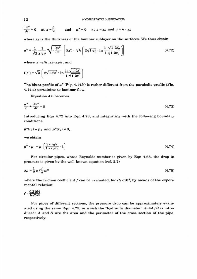
8/9/2019 Hydrostatic Lubrication 1992
http://slidepdf.com/reader/full/hydrostatic-lubrication-1992 99/558
8 2
HYDROSTATIC LUBRICATION
where zo is the thickness of the laminar sublayer on the surfaces. We thus obtain
(4.72)
where
z '=z lh ,
zb=zdh, and
The blunt profile of u* (Fig. 4.14.b) is rather different from the parabolic profile (Fig.
4.14.a) pertaining
t o
laminar flow.
Equation 4.8 becomes
u* au*
- + -=o
r ar
(4.73)
Introducing Eqn 4.72 into Eqn 4.73, and integrating with the following boundary
conditions
we obtain
1
- rz/r
P*
-PI =PI[-- 11
(4.74)
For circular pipes, whose Reynolds number is given by Eqn 4.68, the drop in
pressure is given by the well-known equation (ref. 2.7)
where the friction coefficient
f
can be evaluated, for ReelO5, by means of the experi-
mental relation:
For pipes of different sections, the pressure drop can be approximately evalu-
ated using the same Eqn. 4.75, in which the "hydraulic diameter"
d=4AIS
is
intro-
duced:
A
and
S
are the area and the perimeter of the cross section of the pipe,
respectively.

8/9/2019 Hydrostatic Lubrication 1992
http://slidepdf.com/reader/full/hydrostatic-lubrication-1992 100/558
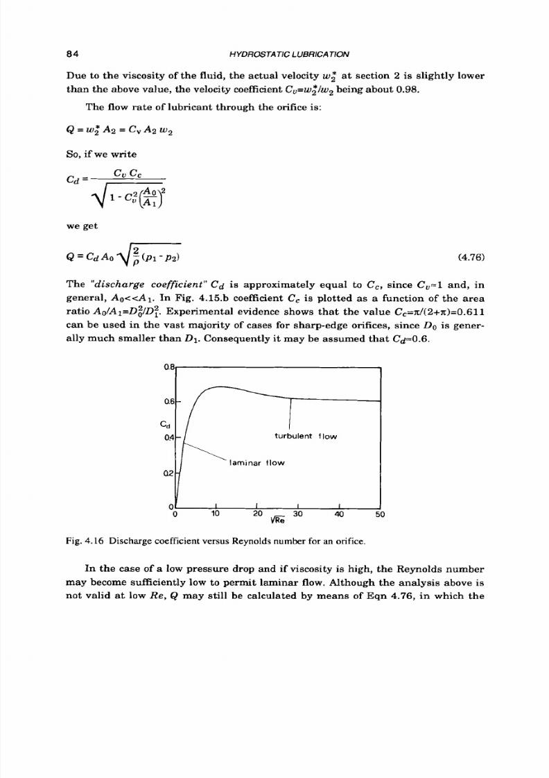
8/9/2019 Hydrostatic Lubrication 1992
http://slidepdf.com/reader/full/hydrostatic-lubrication-1992 101/558

8/9/2019 Hydrostatic Lubrication 1992
http://slidepdf.com/reader/full/hydrostatic-lubrication-1992 102/558
BASIC EQUATlONS 85
discharge coefficient
Cd
is now given in Fig.
4.16.
The initial value of
Re
has to be
calculated for Cd=0.6.
The sharp-edge orifices are sometimes substituted by less costly orifices (Fig.
4.17)
whose length
1
is no longer negligible. In such cases, the discharge coefficient
can be calculated by means of the following equations (ref.
2.7):
1 m -m
Cd = [ .5 + 13.74 a)
for
?<50
;
(4.77)
the relevant values of
Cd
also being plotted in Fig.
4.16.
Re
has to be initially obtained
from Eqn 4.68, with Q being taken from Eqn 4.76 for Cd=0.6.
Since Cd is now a function of the Reynolds number, the flow rate for any certain
pressure step is no longer completely independent from variations in temperature
and viscosity.
0 s
1
o,61
.4
c d
a2
I I
I
1
lo*Re
/
I lo3
.14 10
Fig. 4.17
Discharge coefficient for a short-tube
orif ice.
4
R E F E R E N C E S
4.1
4 3
4 5
4.4
Goldstein S.
D.; Modern Deuelopments in Fluid Dynamics;
Claredon Press,
Oxford, 1952; 702 pp.
Pinkus O., Sternlicht B.; Theory of Hydrodynamic Lubrication; McGraw-Hill
Book Co., N.Y.,
1961; 465
pp.
Tipei
N.;
Theory
of
Lubrication;
Standford Univ. Press,
1962; 690
pp.
Cameron A,; The Principle of Lubricatioq; Longmans, Green and Co. Ltd.,
1966; 591
pp.

8/9/2019 Hydrostatic Lubrication 1992
http://slidepdf.com/reader/full/hydrostatic-lubrication-1992 103/558
86 HYDROSTATIC LUBRICATION
4.6 Shinkle J. N., Hornung V . G.;
Frictional Characteristics
of
Liquid Hydro-
static Bearings;ASME Trans.,J . of Basic Eng., 87 (19651,163-169.
4.6 Ettles
C.
H. M., O'Donoghue
J .
P.; Lam inar Recess Flow in Liquid Hydro-
static Bearings; Instn. Mech. Engrs., C27 (19711,215-227.
4.7 Tipei N.;
Flow Characteristics and Pressure Head Bu ild -up at the Inlet
of
Narrow Passages;
ASME Trans.,J . Lubr. Tech., 100 (1978), 47-55.
4.8 El-Sherbiny M., Salem F . , El-Efnawy N.; Op timum Design of Hydrostatic
Journal Bearings;
Tribology International, 17 (19841, 155-166.
4.9 Langhaar H. L.;
Steady Flow i n the Transition Length
of
a straight Tube;
J . o f
Applied Mech.,9,2 (19421, A55-A58.
4.10 Streeter V.;Handbook
of
Fluid Dynamics; McGraw-Hill, 1961.
4.11 Bassani R.;
Su l Regime Turbolento nei Cu scinetti Zdrostatici d i S pin ta M olto
Caricati;Atti 1st. Mecc Appl. e Costr. Macch., 1968-69,
N
15; 36 pp.

8/9/2019 Hydrostatic Lubrication 1992
http://slidepdf.com/reader/full/hydrostatic-lubrication-1992 104/558
Chapter
5
PAD
COEFFICIENTS
5.1
INTRODUCTION
In this chapter, generalized equations for load capacity W, stiffness
K, low
rate
Q, pumping power
H p ,
friction power
H f
and total power
H t
are proposed, which are
valid for every type of pad. In order t o simplify the representation of the behavior
of
bearings and make their design easier, use is made
of
characteristic parameters,
such as the
effective area A,
and the
hydraulic resistance
R , as well as of the power
ratio ll and the pressure ratio /J
For
the same purpose, certain pad coef f ic ients
(A*,
,R * ,
H F ) are introduced, which are characteristics of the actual pad shape.
They are also considered the effects on the bearing behavior of misalignment
and of certain phenomena, such as turbulence, inlet pressure losses and lubricant
inertia, which are not typical
of
plain hydrostatic lubrication.
5.2
GENERAL STATEMENTS
Whatever the shape of the bearing pads and the supply system, certain general
expressions may be stated. The load capacity of a pad (the resultant of the lubricant
pressure in the bearing) may be put in the following form:
W = Pr A,
(5.1)
p r
is the recess pressure;
A,
is the
“effective“
pad area. This last is a fraction of the
projected area and, in general, depends on the operating conditions; in the most
common cases, however, A, may be considered as a constant, related solely t o the
shape and size of the pad.
8/9/2019 Hydrostatic Lubrication 1992
http://slidepdf.com/reader/full/hydrostatic-lubrication-1992 105/558

8/9/2019 Hydrostatic Lubrication 1992
http://slidepdf.com/reader/full/hydrostatic-lubrication-1992 106/558
PAD
COEFFlClENTS 89
For a fast (and safe) evaluation of AT it is often assumed that all the dissipated
power H , remains in the lubricant (adiabatic flow). As a consequence, we have
simply
(5.7)
where c is the specific heat of the lubricant, and
p
is i ts density (for further discus-
sion on thermal running see chapter 12). The term
H f I H ,
is commonly called the
"power ratio and has also been used (ref. 1.9) for the following grading of hydro-
static bearings: H f / H p = O , zero-speed bearings (purely hydrostatic bearings);
H f I H p < l , lowlmoderate speed bearings; and H f / H p > l , moderate/high speed bear-
ings. In the last case, for certain bearings (e.g. journal bearings), hydrodynamic
load capacity may become important (hybrid bearings).
The static "stiffness" K may be generally defined as the limit of the ratio of a
small change A F of the applied load t o the consequent displacement Ae
of
the mov-
ing member in the direction of the load. In steady-state conditions the external load
F
is balanced by the resultant
W
of the pressure of the lubricant,
so
the stiffness
of
the bearing may be defined as:
For a single-pad thrust bearing, if we use h t o indicate the component of the film
thickness along the direction of the load, we clearly have Ah=Ae, and hence Eqn 5.8
becomes
K=--W
dh
It is important to note tha t the derivative on the right-hand side of Eqn 5.8 is a
total derivative. Indeed,
W
is proportional to recess pressure; this is linked to the
flow rate and to the thickness of the film by a relationship which depends on the
supply system and the compensating devices. For this reason this point will be
examined more closely in sections 6.2 and 6.3.
Once a design value ho has been selected for the clearance of any given pad bear-
ing, it may be worthwhile writing the expressions of each of the foregoing parame-
ters as the product of the value of the parameter in the reference configuration h=ho
times a function of the non-dimensional film thickness h l h , or of the non-dimen-
sional displacement
h - ho
h0
E=-
(5.9)
8/9/2019 Hydrostatic Lubrication 1992
http://slidepdf.com/reader/full/hydrostatic-lubrication-1992 107/558
90 HYDROSTATIC LUBRICATION
It should be noted that fqr certain types of pad a "natural" reference configura-
tion exists (e.g. the concentric configuration for the cylindrical o r spherical pads).
In non-dimensional form, hydraulic resistance
R
and friction power
H f
can
now be rewritten as:
R = R o R ' (5.10)
R o and
Hf o
being the relevant reference values. For the pads whose clearances have
an uniform thickness the results obtained in Chapter 4 allow
us
to write:
(5.12)
(5.13)
The stiffness may also be written in the form:
K = K o K
(5.14)
but now both KOand K' are dependent on the supply system, and will be defined
later.
One parameter which will be widely used in the following chapters is the
"pressure ratio" in the reference configuration:
(5.15)
Another important parameter t o take into consideration
is
the "referencepower
ratio", that is the power ratio in the reference configuration:
The importance of this parameter consists in the fact that it provides a simple but
effective way
of
optimizing the selection of the lubricant and of the clearance, as will
be shown later.
In order to evaluate the actual bearing performance, it is now necessary:
t o
evaluate the foregoing parameters for the main types of pad; this will be
done in the remainder of this chapter;
to establish the relationship between the
flow
rate, the recess pressure and the
supply pressure for the most common supply systems. This will be done in section

8/9/2019 Hydrostatic Lubrication 1992
http://slidepdf.com/reader/full/hydrostatic-lubrication-1992 108/558
PAD
COEFFICIENTS
91
6.2 (for
the
"direc t"
supply system) and section
6.3
(for the
"compensated"
supply
systems).
5.3
CIRCULAR RECESS PAD
5.3.1
Basic equations
A set of equations, with which the parameters
of
the simple bearing in Fig.
5.1.a
may be calculated, have been already obtained in section
4.7.5.
In particular,
it
was
found there that the
flow
rate Q and the load capacity
W
(written as functions
of
the
recess pressure
p r )
are
(5.17)
(5.18)
where
is the ratio of the inner radius
of
the land surface to the outer one. Comparing these
equations
to
Eqn
5.1
and Eqn
5.2,
the effective pad area and the hydraulic resistance
are easily obtained:
(5.20)
A,
=
4 Dz A
R=:$R*
A*,and R*, which are plotted in Fig. 5.l.b, are:
(5.21)
(5.22)
R* = In llr'
(5.23)
The pumping power dissipated in the bearing is given by Eqn 5.4. It may prove
useful t o express it as a function of the load capacity:
(5.24)
where
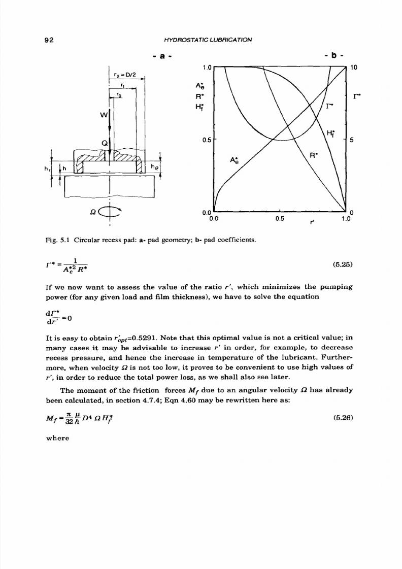
8/9/2019 Hydrostatic Lubrication 1992
http://slidepdf.com/reader/full/hydrostatic-lubrication-1992 109/558
92
HYDROSTATlC LUBRlCATlON
- b -
a -
h
10
r
5
3
Fig. 5.1 Circular recess pad: a- pad geomc y;
b-
pad coefficients.
(5.25)
r*=AT
If we now want
t o
assess the value of the ratio r’, which minimizes the pumping
power (for any given load and film thickness), we have to solve the equation
It
is
easy to obtain
r&,=0.5291.
Note that this optimal value
is
not
a
critical value; in
many cases i t may be advisable to increase
r’
in order, for example, to decrease
recess pressure, and hence the increase in temperature of the lubricant. Further-
more, when velocity Q is not too low, it proves to be convenient to use high values of
r‘, in order to reduce the total power loss, as we shall also see later.
The moment of the friction forces Mi due
to
an angular velocity R has already
been calculated, in section4.7.4; qn 4.60may be rewritten here as:
where

8/9/2019 Hydrostatic Lubrication 1992
http://slidepdf.com/reader/full/hydrostatic-lubrication-1992 110/558
PAD
COEFFICIENTS
93
Fig. 5.2
Nomograph for
a circular
pad.
8/9/2019 Hydrostatic Lubrication 1992
http://slidepdf.com/reader/full/hydrostatic-lubrication-1992 111/558
94
HYDROSTATIC LUBRICATION
is
plotted in Fig. 5.1.b. The friction power is:
H f = Q M = E E D 4 Q 2 H f * (5.28)
The friction coefficient, referred
to
the mean radius of the land P=(rl+r2)/2, is
f
32h
(5.29)
It can be shown (ref. 5.1) that, for moderate speeds, can be as little
as 0.01
times the
friction coefficient of the rolling bearings.
EXAMPLE 5.1
A pad bearing, which has to carry a load W=20,000 N, rotates at a speed Q=2n
radls (i.e. 60 rpm); its external diameter is D=O.l m. The lubricant viscosity, at a
working temperature
T=4OoC,
s p=O.l Ns im2. For the ratio
re ,
the optimal value
is chosen: rAPt=0.53, because of low velocity. For the f i lm thickness the value h=50
pm is chosen in order to avoid the influence of errors in parallelism (see section
5.3.3).
Let us calculate the main bearing parameters. From Eqn 5.22
or
from Fig. 5.1.b
it is easy to obtain
Af
=0.566 and hence the ef fective area is (from Eqn 5.23)
A,=4.45.10-3 mz. As a consequence, the recess pressure which is needed to sustain
the design load is (from Eqn 5.1) pr=4.5 MPa.
From Eqn 5.23,
or from Fig. 5.1.b, we find R*=0.635, and a hydraulic resistance
(Eqn 5.21) RO=970.10sNsIm5. From Eqn 5.2 it immediately follows that the flow rate
which is required to sustain the load with the planned clearance is &=4.63.10-6
m3Is.
The pumping power dissipated in the bearing is Hi=prQ=20.8 W : for a direct
supply system (i.e. &=const,ps=pr) this is also the actual pumping power. Equation
5.27, or Fig. 5.1.b, gives Hf*=0.921. The friction power is obtained from Eqn 5.28:
Hf=O.714
W;
this low value justifies the choice of
r'=rApt.
The friction moment is
Mf=Hf/LkO.114N m and the friction coefficient (Eqn 5.29) i s f=0.149.10-3
5.3.2
Design chart
For the calculus of a circular-recess hydrostatic thrust bearing, it may prove
worthwhile to use, as a
first
approach, the design chart in Fig. 5.2.) obtained from
Eqn 5.17 and Eqn 5.18 rewritten in logarithmic form. It allows us t o obtain the main
design parameters of a bearing in graphical form. By way of example, let us con-
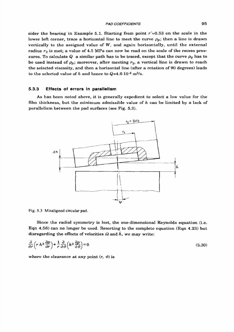
8/9/2019 Hydrostatic Lubrication 1992
http://slidepdf.com/reader/full/hydrostatic-lubrication-1992 112/558
PAD
COEFFICIENTS 95
sider the bearing in Example 5.1.Starting from point
r’=0.53
on the scale in the
lower left corner, trace
a
horizontal line
t o
meet the curve
p,;
then a line is drawn
vertically t o the assigned value of
W,
and again horizontally, until the external
radius
r2
is met;
a
value of
4.5
MPa can now be read on the scale
of
the recess pres-
sures. To calculate
Q a
similar path has to be traced, except that the curve
pq
has to
be used instead
of p,;
moreover, after meeting
r2 ,
a vertical line is drawn to reach
the selected viscosity, and then a horizontal line (after a rotation of 90 degrees) leads
to the selected value of h and hence to
&=4.6.10-6
m%.
5.3.3 Effects of errors
i n
paral lel ism
As has been noted above, it is generally expedient to select a low value for the
film thickness, but the minimum admissible value of h can be limited by a lack of
parallelism between the pad surfaces (see Fig. 5.3).
Fig.
5.3
Misaligned circular pad.
Since the radial symmetry is lost, the one-dimensional Reynolds equation (i.e.
Eqn 4.56) can no longer be used. Resorting to the complete equation (Eqn 4.23) but
disregarding the effects of velocities R and A we may write:
(5.30)
where the clearance a t any point (r , ts) is
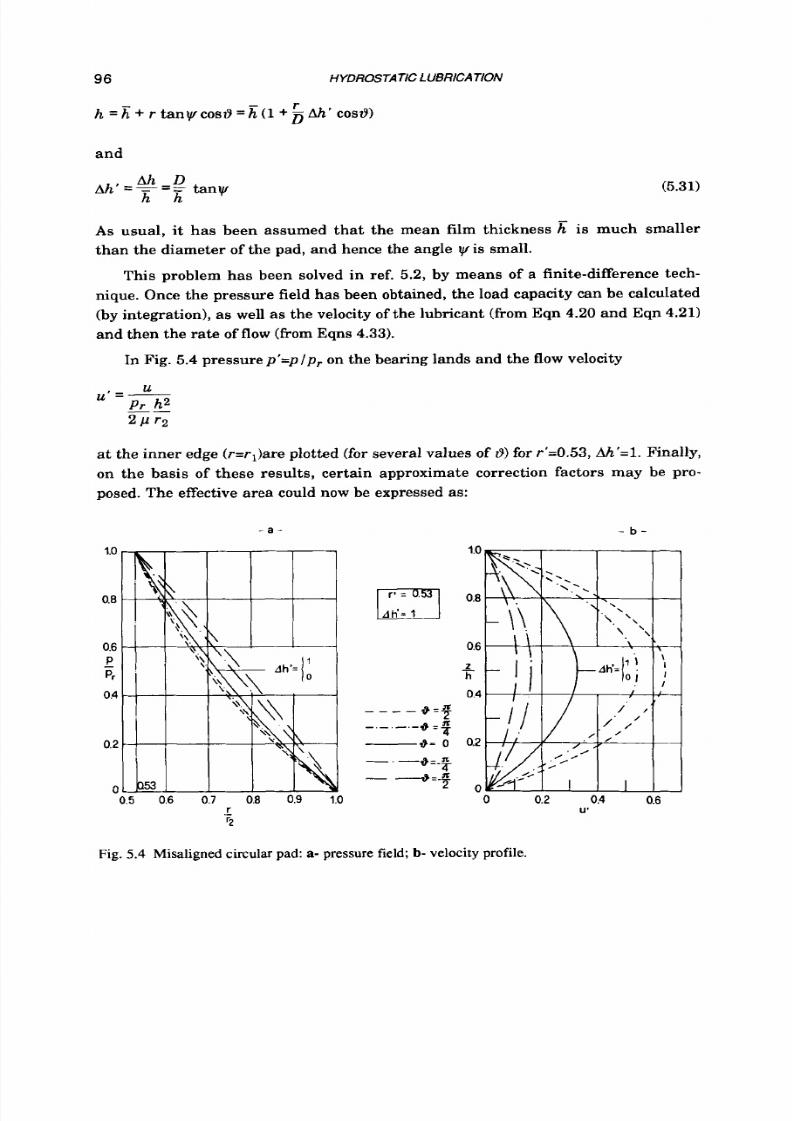
8/9/2019 Hydrostatic Lubrication 1992
http://slidepdf.com/reader/full/hydrostatic-lubrication-1992 113/558
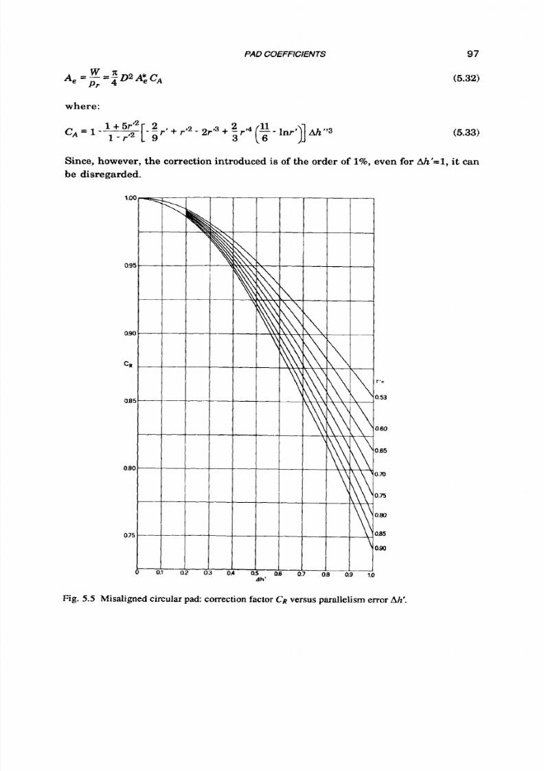
8/9/2019 Hydrostatic Lubrication 1992
http://slidepdf.com/reader/full/hydrostatic-lubrication-1992 114/558
PAD
COEFFICIENTS
where:
Since, however, the correction introduced is of the order of 1%,
be disregarded.
0.8
0.9
1
97
(5.32)
(5.33)
even for Ah’=l, it can
res
0.53
0.60
0.65
0.m
0.75
0.80
085
090
Fig. 5.5 Misaligned circular pad: correction factorCR ersus parallelism error Ah‘.
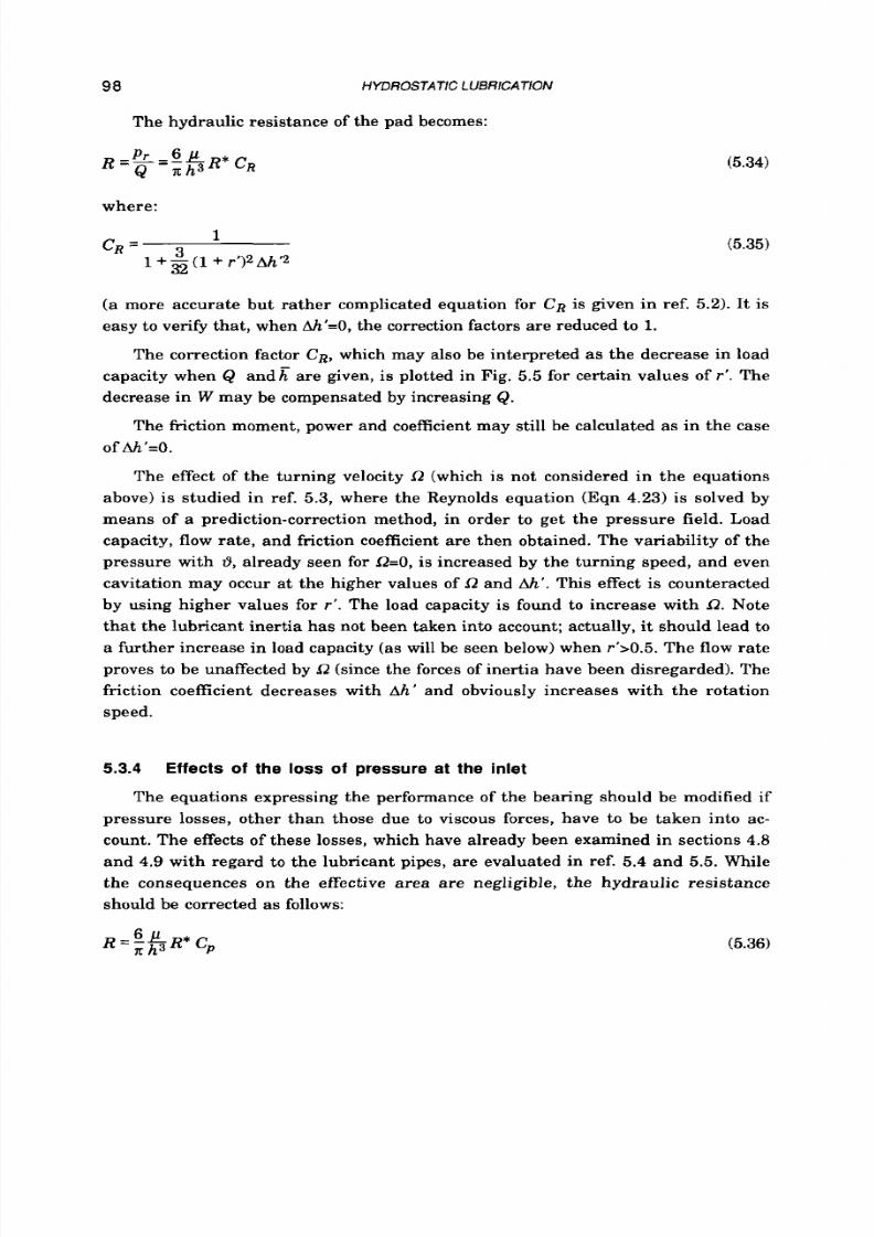
8/9/2019 Hydrostatic Lubrication 1992
http://slidepdf.com/reader/full/hydrostatic-lubrication-1992 115/558
98 HYDROSTATC
LUBRlCATlON
The hydraulic resistance of the pad becomes:
where:
1
l+g l
r ’ )ZAh‘2
c R = 3
(5.34)
(5.35)
(a more accurate but rather complicated equation for CR s given in ref.
5.2).
It is
easy t o verify that , when Ah’=@ the correction factors are reduced to 1.
The correction factor C,, which may also be interpreted as the decrease in load
capacity when Q an dx are given, is plotted in Fig. 5.5 for certain values of r ’ . The
decrease in W may be compensated by increasing Q.
The friction moment, power and coefficient may still be calculated as in the case
ofM’=O.
The effect of the turning velocity R (which is not considered in the equations
above) is studied in ref. 5.3,where the Reynolds equation (Eqn 4.23) s solved by
means of a prediction-correction method, in order to get the pressure field. Load
capacity, flow rate, and friction coeficient are then obtained. The variability of the
pressure with
19,
already seen for
R=O,
is increased by the turning speed, and even
cavitation may occur at the higher values of R and Ah’. This effect is counteracted
by using higher values for r ‘ . The load capacity is found to increase with R. Note
that the lubricant inertia has not been taken into account; actually,
it
should lead to
a further increase in load capacity (as will be seen below) when rb0.5 . The flow rate
proves to be unaffected by
R
(since the forces of inertia have been disregarded). The
friction coefficient decreases with
Ah
’ and obviously increases with the rotation
speed.
5.3.4
Effects of the l oss of pressure at the in let
The equations expressing the performance of the bearing should be modified if
pressure losses, other than those due
t o
viscous forces, have to be taken into ac-
count. The effects of these losses, which have already been examined in sections 4.8
and 4.9 with regard t o the lubricant pipes, are evaluated in ref. 5.4 and 5.5. While
the consequences on the effective area are negligible, the hydraulic resistance
should be corrected as follows:
(5.36)

8/9/2019 Hydrostatic Lubrication 1992
http://slidepdf.com/reader/full/hydrostatic-lubrication-1992 116/558
PAD COEff /C/ENTS
99
Fig.
5.6 Pressure losses
at
the
inlet
of clearance: correction factor
C pfor
circular
pads.
where the correction factor
C p
is given by the equation:
(5.37)
and R e is the Reynolds number (Eqn 4.61); F=(Fl+F2)/2
is
the mean radius of the
land surface; ti,. is the inlet length:
(5.38)
The first term of the numerator in Eqn 5.37 takes into account the pressure
losses due to the viscous forces in the bearing gaps; the second stands for the energy

8/9/2019 Hydrostatic Lubrication 1992
http://slidepdf.com/reader/full/hydrostatic-lubrication-1992 117/558
100 HYDROSTATIC LUBRICATION
used to accelerate the fluid in the inlet zone; the third term represents the contrac-
tion loss. Equation 5.38 of the inlet length is valid for
Ar=r2-r121ir;
or greater values
of
l ir,
one can simply substitute
Ar
for l i , in Eqn 5.37, unless (in which case
the bearing gap would virtually behave a s
an
orifice ). Coefficients
k l , k 2 ,
and
k3
are
obtained in ref. 5.5 from the experimental data given in ref. 5.4, with the following
values: k1=0.75, k2=0.235,and k3=0.021;thus the correction factor for
R
becomes
C p = l + - -
0.0313 2 + 0.00979
1
1 (l+l/rY
1 +0.00525l n p
_ -
h Re
(5.39)
It is plotted in Fig.
5.6
as a function of
Arl(h.Re)
for a number of values of
r'.
Unlike the case of error in parallelism, the inlet losses have favorable effects.
These effects would be rather important for very small (~0 .1 )alues of Arl(h.Re),
which are, however, unusual in actual fact.
The coefficient
C p
may also be explained as a n increase in load capacity, for any
given flow
rate,
o r as a decrease in flow rate, for any given load.
It
should be noted
that C, becomes considerable in the case of ArchaRe.
EXAMPLE 5.2
A circular pad bearing, whose diameter is D=O.l m, has been selected to sustain
a load W=50 Mv rotating at 750 rpm (i2=251r radls). Furthermore, the recess pres-
sure needs to be smaller than 7.2 MPa and the friction torque needs to
be
smaller
than 0.05 Nm. Let us assess the flow rate, assuming that a lubricant with p=O.O18
Ns lm2 and p=880Kglm3 must be used.
From the condition p,<7.2 MPa, it follows that Ae>6.94.10-3m2(Eqn 5.1), and
Az>0.884 (Eqn 5.20). From Fig. 5.1.6 a radius ratio of about 0.9 seems to be neehd. I f
we select r'=0.9,we easily obtain A50.902, R*=0.105, Hf*=0.344. The effective area is
then
Ae=7.08.103
m2,
and hence the recess pressure will be p,=7.06 MPa.
Since necessarily Mf<0.05 Nm, it follows from Eqn 5.26 hat
h95 .5
pm. If a
clearance h=100 pm is selected, it follows that R=3.62.109 NslmS (Eqn 5.21) and
Q=1.95.10-3 m31s. Since Q is high, it is advisable to verify the effect of the pressure
losses at the inlet. From Eqn 4.61, the Reynolds number is Re=319 and, from Fig.
4.6, Cp=1.26. Hence, the new value of the flow rate is calculated: Q=1.54.10-3 m3/s.
This is still a high value; it should be borne in mind, however, that a very low fric-
tion was required, the friction coefficient being of the order of 2.10-5.

8/9/2019 Hydrostatic Lubrication 1992
http://slidepdf.com/reader/full/hydrostatic-lubrication-1992 118/558
PAD COEFFICIENTS 101
5.3.5
Turbulent f low
Although the
flow
in the clearances
of
hydrostatic bearings is, generally, of a
laminar type, in certain circumstances (as already noted in section 4.10) the
Reynolds number (Eqn 4.61) may become greater than 2300, a t which value the flow
is prevalently turbulent. Equations giving pressure and lubricant velocity in the
clearance of a circular pad in turbulent regime have been obtained in section 4.10.
Integrating the mean pressure (Eqn
4.74)
on both the recess and land area, the
load capacity proves
to
be:
(5.40)
W
=
4
D2
r'p ,
while, if we integrate the radial velocity field (Eqn
4.72),
the following flow rate
is
obtained:
where (ref. 4.11):
and
(5.42)
(5.43)
The nondimensional quantities x and A (which depends on zb and accounts for the
rate
of
flow
in the laminar boundary sublayer along the land surfaces) are evalu-
ated in ref. 4.11, for Re>2300:
Comparing Eqn 5.40 and Eqn 5.41 with those obtained for the laminar flow, two
correction factors are easily obtained for the effective area as well as the hydraulic
resistance
of
the pad. After stating that:
(5.44)
(5.45)

8/9/2019 Hydrostatic Lubrication 1992
http://slidepdf.com/reader/full/hydrostatic-lubrication-1992 119/558
102
it
follows that:
HYOROSTATIC LUB RICA
TION
(5.47)
When r’ is greater than 0.80, we have 0 .9 9 <C ~ ~< l,nd hence
CAT
may be disre-
garded; furthermore, for r’>0.5, we have 6 % ~ ) l n ( l / r 7 , hus
(5.48)
‘RT
O X 5 ( l + A ) zb F(zb)
and, hence, CRT may be considered t o depend on zb alone. Both CAT and CRT re
plotted in Fig. 5.7.
- a - - b -
1
oo
CAT
0.95
0.90
0.50
0.75
1
oo
f
10
CRT
5
0
0.00 0.05
0.10
zb
Fig.
5.7
Turbulent flow: a- correction factor
CAT
or effective area; b- correction factor C,, for
hydraulic resistance.
Since CRT roves t o be greater than 1,we can see that, at high Reynolds numbers,
turbulence brings about a considerable decrease in flow rate or, if
flow
rate remains
constant, a considerable increase in load capacity. On the other hand, turbulence
may cause a large increase of foam in the lubricant; the persistence of the foam

8/9/2019 Hydrostatic Lubrication 1992
http://slidepdf.com/reader/full/hydrostatic-lubrication-1992 120/558
PAD COEFFICIENTS
103
depends on the physico-chemical properties
of
the oils, and may be counteracted by
means of suitable anti-foam additives (see chapter
3).
EXAMPLE
5.3
Let us re-examine the hydrostatic pad in Exumple 5.2,
in
order to evaluate how
the flow rate would vary if the clearance and the viscosity were changed to h=200
pm and p=0.005 Ns
Im2
( I S 0 VG5), espectively.
From
Eqn 5.21 it follows that R=O.126.1@ NslmS, and hence Q=56.1.10-3 m31s.
Since the Reynolds number proves to be greater than 2300 (Eqn 4.61), a correction
factor should clearly be evaluated. From Eqn 5.42 we obtain z&0.0112, and hence
C~,=7.78, R=0.979.109
Nslm5,
Q=7.23.103 m3/s (in spite
of
the considerable reduc-
tion due to turbulence, this is a very high value). The Reynolds number proves to be
Re54260.
Bearing in mind the above results, it may be concluded that, for values
of
Re
lower than 10, which is the most common case for these hydrostatic thrust bear-
ings, the whole pressure loss in the clearance is due t o viscous forces; when
Re
is
greater than 100, the pressure losses examined in section (v) become considerable;
when Re is greater than 1000, the effect of turbulence should be taken into account.
In both these cases, for any given load capacity and
film
thickness, the flow rate
proves
t o
be lower than that expected
on
the basis of the laminar theory.
5.3.6 Effects of the inertia forces
When the angular speed of the bearing in Fig. 5.1.a is high, the forces of inertia
in the fluid can no longer be disregarded. Supposing h=const, but retaining the
inert ia term, Eqn 4.23 becomes:
where the “inertia parameter”
(5.49)
(5.50)
has been introduced.
This kind
of
problem has been solved in ref. 5.6. When
r o o l ,
he depth h,. of the
recess should be
at
least 5 imes greater than the film thickness h , while hr=20h is
considered t o be a n optimal value.
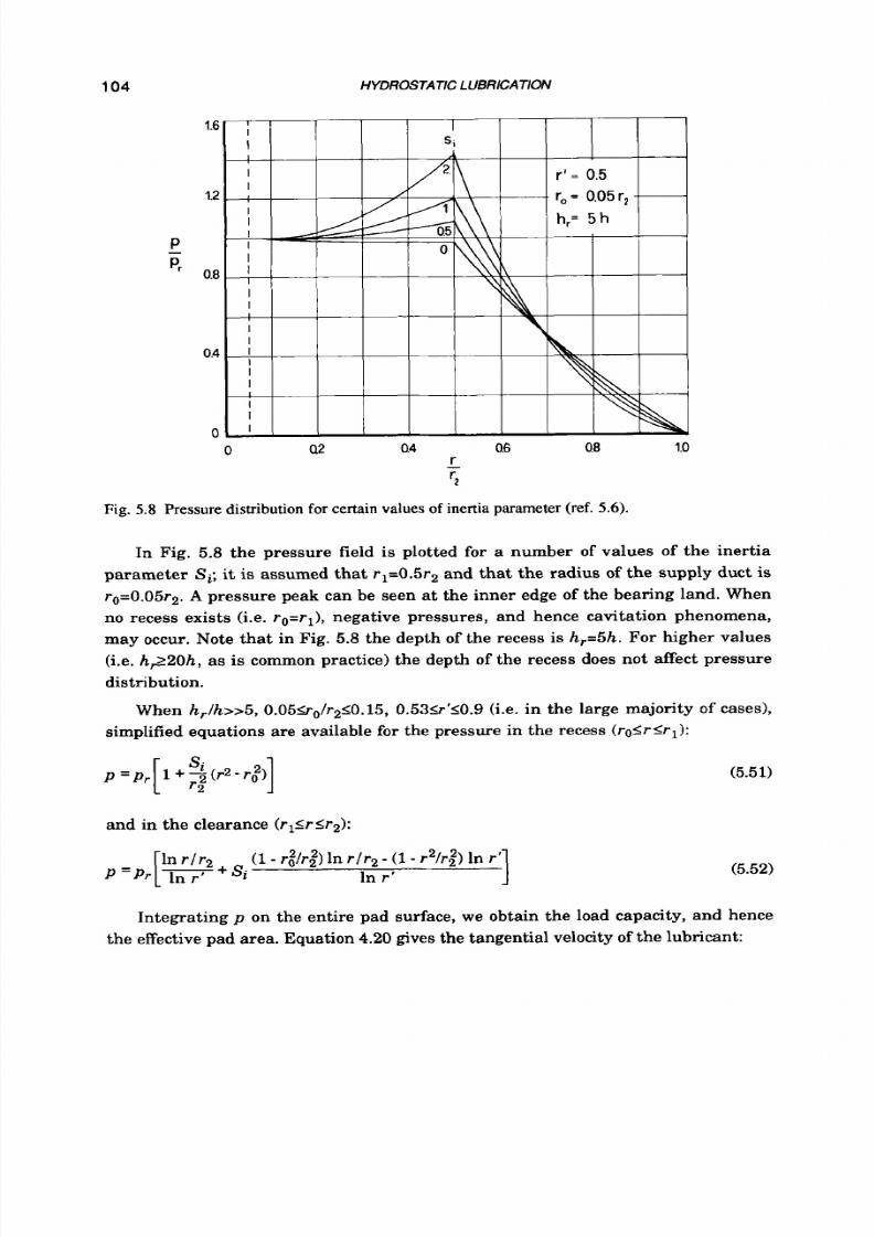
8/9/2019 Hydrostatic Lubrication 1992
http://slidepdf.com/reader/full/hydrostatic-lubrication-1992 121/558
104
HYDROSTATIC LUBRICATION
Fig. 5.8 Pressure distribution for certain values
of
inertia parameter (ref. 5.6).
In Fig.
5.8
the pressure field
is
plotted
for
a number
of
values
of
the inertia
parameter Si; t is assumed that r1=0.5r2and that the radius of the supply duct
is
ro=0.05r2.A pressure peak can be seen at the inner edge of the bearing land. When
no recess exists (i.e.
r o = r l ) ,
negative pressures, and hence cavitation phenomena,
may occur. Note that in Fig. 5.8 the depth of the recess is h,=5h. For higher values
(i.e. h,.220h, as
is
common practice) the depth of the recess does not affect pressure
distribution.
When h,/h>>5, 0 .05~ , / r2<0 .5, 0.534'10.9 i.e. in the large majority of cases),
simplified equations are available
for
the pressure in the recess
fro<rlrl):
(5.51)
and in the clearance
( r l < r < r 2 ) :
(5.52)
Integrating
p
on the entire pad surface,
we
obtain the load capacity, and hence
the effective pad area. Equation 4.20 gives the tangential velocity of the lubricant:

8/9/2019 Hydrostatic Lubrication 1992
http://slidepdf.com/reader/full/hydrostatic-lubrication-1992 122/558
PAD
COEFFICIENTS
105
Since
u
a n d p are now known functions, the radial flow velocity, an d hence the
volume flow rate, may now be easily obtained from Eqn
4.21.
The effective area and the hydraulic resistance may thus be expressed
as
R = : $ R * cRI
where:
c , = l + s i [(
1- - )
+
(1--
1
CRI
=
1
+
si1
-3)
It is clear, however,
that
c,=1+si 1---
(
2
1
CRI
=
(5.53)
(5.54)
(5.55)
(5.56)
(5.57)
(5.58)
are very good approximations in the large majority of cases. In Fig. 5.9 CAI,is given
as a function of Si for certain values of F'. In the same
figure
CRI is also given as a
function of
Si.
The increase in flow rate (the inverse of C R I )may be appreciable even for mod-
era te values of the inertia parameter. I t is moderately compensated by the increase
in load capacity (i.e. C,). Since
C
increases with Si, oad capacity W is increased
by inertia effects if inlet pressure is held constant; thus these bearings are often
named hybr id. However, as CRI simultaneously decreases more quickly, flow rate Q
increases more greatly than W, so an efficiency loss of the bearing may occur.
The Reynolds number, as given by Eqn
4.61, is
usually very low. Nevertheless,
turbulence could set in, due
to the tangential flow velocity. In ref. 5.10, in which the
circular pad
is
compared
t o
the case of
a
couple of faced rotating
disks
(ref.
5.71,
the
Reynolds number R e , = a r ; /
v
is introduced, and the flow is proved to be laminar for
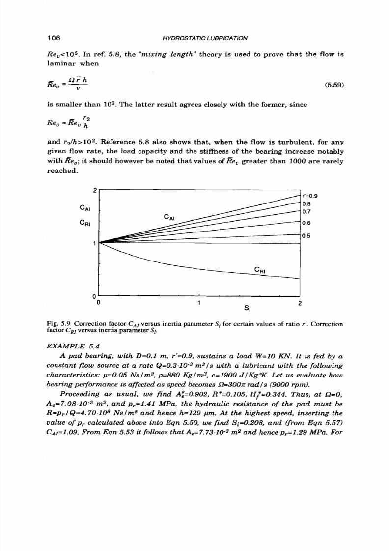
8/9/2019 Hydrostatic Lubrication 1992
http://slidepdf.com/reader/full/hydrostatic-lubrication-1992 123/558
106 HYDROSTATIC LUBRICATION
Re,<lO5. In ref.
5.8,
the “mixing length” theory is used to prove that the flow is
laminar when
L?Fh
Re,
=
(5.59)
is smaller than lo3.The latter result agrees closely with the former, since
r2
Re,
=: Re,
and r2/h>102. Reference
5.8
also shows that, when the flow is turbulent, for any
given flow
rate,
the load capacity and the stiffness of the bearing increase notably
with
Re,;
it
should however be noted tha t values of
Re,
greater than
1000
are rarely
reached.
i
CAI
CRI
1
0
0
f=0.9
0.8
0.7
0.6
0.5
1
2
Si
Fig.
5.9
Correction factor
CA,
versus inertia parameter
Si
for certain values of ratio
r‘.
Correction
factor CRI ersus inertia parameter
Sk
EXAMPLE 5.4
A pad bearing, with D=O.l m, r’=0.9, sustains a load W=lO
Mv.
It is fed by a
constant flow source at a rate &=0.3.1O3 m 3/ s with a lubricant with the following
characteristics: p=0.05Nslm2,
p=880
Kglm3, c=1900 JIK&jC Let
us
evaluate how
bearing performance is affected
as
speed becomes
G30Oz
rad Is (9000 rpm).
Proceeding as usual, we f ind Az=0.902, R*=0.105, Hf*=0.344. Thus, at Q=O,
Ae=7.08.10-3m2, and p,=1.41 MPa, the hydraulic resistance o f the pad must be
R=p,l&=4.70.1O9 Nslm5 and hence h=129 pm. At the highest speed, inserting the
value of
pr
calculated above into Eqn
5.50,
we find Si=O.208, and (from Eqn 5.57’
C~ =l .0 9. rom Eqn 5.53 it follows that Ae=7.73.10-3m2 and hencep,=1.29 MPa. For
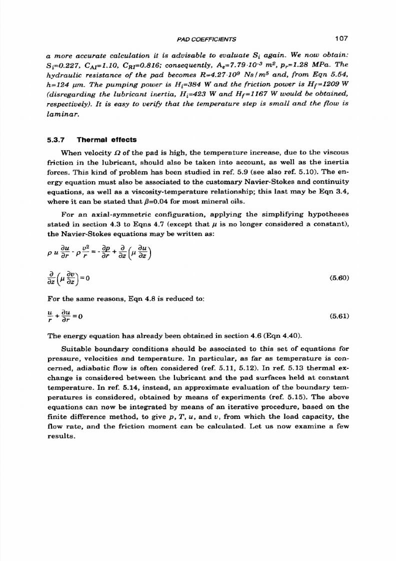
8/9/2019 Hydrostatic Lubrication 1992
http://slidepdf.com/reader/full/hydrostatic-lubrication-1992 124/558
PAD COEFFICIENTS 107
a more accurate calculation it is advisable to evaluate Si again. We now obtain:
S i=0 .227 , CN=l . lO , C~1=0.816;onsequently, A,= 7.79.1 0-3 m2, p,=1 .28 M Pa. The
hydraulic resis tance
of
the pad becomes R=4.27,1O9 N sl m 5 an d, from Eqn 5.54,
h=124 pm . The pumping power is Hi=384 W a n d the fr ic tion power is Hf= 120 9
W
(disregarding the lubricant inertia, Hi=423
W
and Hf=1167 W would
be
obtained,
respectively).
It
is easy to verifv that the temperature step is small and the flow is
laminar .
5.3.7 Thermal
effects
When velocity L? f the pad is high, the temperature increase, due to the viscous
friction in the lubricant, should also be taken into account, as well as the inertia
forces. This kind of problem has been studied in ref. 5.9 (see also ref. 5.10).The en-
ergy equation must also be associated to the customary Navier-Stokes and continuity
equations, as well as a viscosity-temperature relationship; this last may be Eqn 3.4,
where it can be stated that
p=0.04
or most mineral oils.
For
an axial-symmetric configuration, applying the simplifying hypotheses
stated in section 4.3 o Eqns 4.7 (except that p is no longer considered
a
constant),
the Navier-Stokes equations may be written as:
+$)=o
For the same reasons, Eqn 4.8 is reduced
to:
(5.60)
(5.61)
The energy equation has already been obtained in section
4.6
Eqn
4.40).
Suitable boundary conditions should be associated to this set of equations €or
pressure, velocities and temperature. In particular, as far as temperature is con-
cerned, adiabatic flow is often considered (ref.
5.11,5.12).
In ref.
5.13
hermal ex-
change
is
considered between the lubricant and the pad surfaces held
at
constant
temperature. In ref. 5.14, nstead, an approximate evaluation of the boundary tem-
peratures is considered, obtained by means of experiments (ref. 5.15). The above
equations can now be integrated by means
of
an iterative procedure, based on the
finite difference method, to give
p , T , u ,
and
v ,
from which the load capacity, the
flow rate, and the friction moment can be calculated. Let us now examine a few
results.

8/9/2019 Hydrostatic Lubrication 1992
http://slidepdf.com/reader/full/hydrostatic-lubrication-1992 125/558
108
HYDROSTATIC
LUBRICATION
The temperature field plotted in Fig. 5.10 refers to a lubricant, with a n inlet
temperature T=35'C, in the clearance of a bearing with the following characteris-
tics: r2=0.0657m, r1=0.0348m (r'=0.53),r0=0.006m, h=100 pm, &419 rads, pr=0.294
MPa; the data concerning the lubricant, at
2OoC,
are:
p=0.0645
Ns/m2,
p=857
Kg/m3,
c=1890
J/Kg"K,
~=0.144
W/m°K. The maximum temperature, at r=r2 and
z=0.54h,
is
T=5OoC
with an increase
AT=15OC.
In comparison with the case of isothermal flow,
taking into account inertia effects, pressure in the clearance proves to be slightly
lower. Moreover we have:
W=2190
N,
Q =13.8.10-6
m3/s,
Mf=2.22
Nm. So, compared
to the case of isothermal flow, in which we should have
W=2054
N,
Q =18.3.10-6
m3/s,
Mf=3.2
Nm, the load capacity proves to be
6.2%
lower, the flow rate
24.5%
greater, and the friction moment 30.6%lower. Moreover, in the case of isothermal
flow, from Eqn 5.7, we should have AT=45OC.
34 35 37 3 9 41 43 45 47 49 50
T
( O C )
Fig.
5.10 Temperature distribution in the clearance
of
a circula r pad: r l= 0.0348
m, r2=0.0657
m,
h=lO-4 m,
-19
r d s , r= 0.294 MPa.
As
parameter
Si,
iven by Eqn
5.50,
increases, the deviation from the isothermal
case becomes prominent. For example, for the pad considered above, let us now
suppose f2~628.3ads, pr=98.1 KPa, and hence Si=2.196. The maximum tempera-
ture increase now proves to be AT=45 Ca t r=r2 and z/h=0.8; along the upper pad
surface we have AT=31°C and AT=25.5 Calong the lower surface. The calculated
pressure field is shown in Fig. 5.11, where a negative (relative) pressure (confirmed
experimentally, ref. 5.15) indicates the possibility of cavitation phenomena. More-
over, we have
W=642
N,
Q
=14.6.10-6
m3/s,
Mf=2.25
Nm, and in comparison with
the isothermal case, the load capacity proves to be
33%
lower, the flow rate
68%
greater and the friction moment
55%
lower.
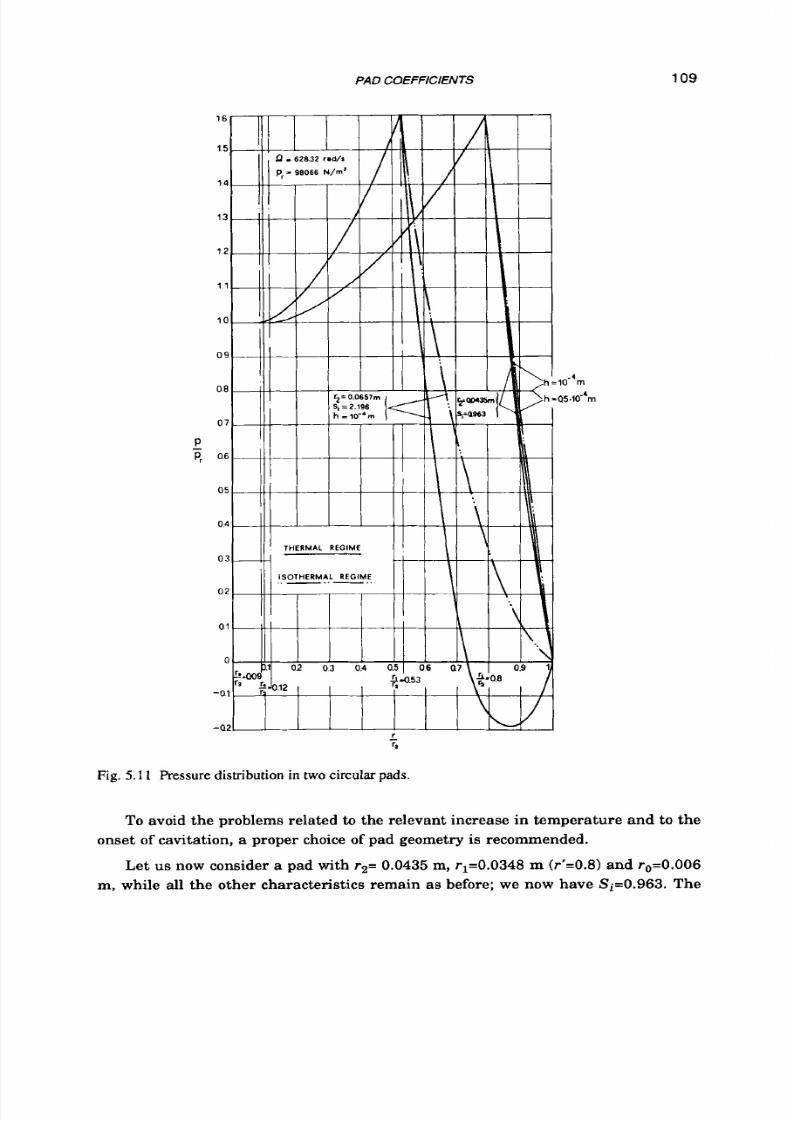
8/9/2019 Hydrostatic Lubrication 1992
http://slidepdf.com/reader/full/hydrostatic-lubrication-1992 126/558

8/9/2019 Hydrostatic Lubrication 1992
http://slidepdf.com/reader/full/hydrostatic-lubrication-1992 127/558
110
HYDROSTATIC LUBRICATION
maximum A T proves t o be lower than 8°C; he pressure pattern (also shown in Fig.
5.11) is very close to the isothermal case, and so obviously occurs for the load capac-
ity W=642 N, while the flow rate Q=17.7.10-6m3/s is greater by 17.4%. In compari-
son with the previous pad, the load capacity
is
similar, but the flow rate
is
even
greater. A possible countermeasure may be a reduction in film thickness. If we take
h=50 pm, the maximum temperature increase proves to be AT=23'C, but the pres-
sure pattern is still close to the isothermal case (Fig. 5.11) and we have W=618 N,
Q=2.43.10-6 m3/s, Mf=0.821 Nm.
So,
due to the thinner clearance, the actual flow
rate proves to be about one 7th of what i t was before.
We must point out it is best to use pads with a small radius and a large recess,
when Q is large. The convenience of large recesses will be demonstrated in section
6.4
and in chapter 11.
All the above results agree closely with those obtained in ref. 5.11 and 5.12 in the
simplifying hypothesis of adiabatic flow. Reference 5.11 suggests that the possibility
of adopting the isothermal theory (ref. 5.6), instead of the adiabatic theory, depends
on the
"viscosity param eter"
where g is the acceleration of gravity. By way of example, for water-lubricated bear-
K '
Fig. 5.12 Correction parameters
kw. k~
and k~ for thermal regime.

8/9/2019 Hydrostatic Lubrication 1992
http://slidepdf.com/reader/full/hydrostatic-lubrication-1992 128/558
PAD COEFFICIENTS
111
ings, V takes on values of about
compared
t o
the mineral oils) and the isothermal theory
is
fairly valid.
(due to the low viscosity and high specific heat,
Although the iterative procedure mentioned above can be quite accurate, it is
still very complicated and does not lead t o any direct expression of pressure, load
capacity, flow rate, and friction moment as functions of the parameters of the pad.
A simpler method is described in ref. 5.16,which is based on using the results con-
tained in ref. 5.14, o obtain an approximate expression of viscosity as a function of
r ,
in the thermo-fluid-dynamic regime. The Navier-Stokes and the continuity equa-
tions are then solved
to
give the pressure field; finally we obtain the following:
(5.62)
(5.63)
(5.64)
5.16
as functions of
(5.65)
and are plotted in Fig.
5.12.
n Eqn
5.65,
l = p ( r l ) ,
Q
, and H f are the values that
these parameters take on in the isothermal case.
The method has been tested for a number of bearings, with k* in the 0.211.3
range, and good agreement was found with the numerical results referred to above
(deviations were smaller than
5%
for
W
and M, nd smaller than 10% for
Q
1. It
should be pointed out that, for
k*<0.2,
the isothermal theory may be applied, while
k*=1.3 s
quite a high value.
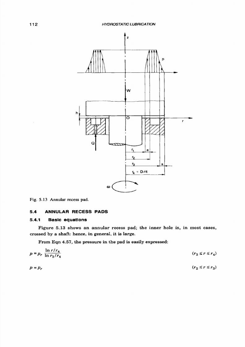
8/9/2019 Hydrostatic Lubrication 1992
http://slidepdf.com/reader/full/hydrostatic-lubrication-1992 129/558
112
HYDROSTATIC LUBRICATION
4
li
Fig. 5.13 Annular recess pad.
5.4 ANNULAR RECESS PADS
5.4.1 Basic
equations
Figure
5.13
shows an annular recess pad; the inner hole is, in most cases,
crossed
by
a shaft: hence, in general, it is large.
From
Eqn
4.57,
the pressure in the pad is easily expressed:
In rlrq
p = p r
P = P r

8/9/2019 Hydrostatic Lubrication 1992
http://slidepdf.com/reader/full/hydrostatic-lubrication-1992 130/558
PAD
COEFFICIENTS
113
In
r l r 2
P = P r
l-w)
(rl I
r
I rz)
Integrating the pressure field on the whole bearing area, we obtain load capac-
ity
W.
Bearing Eqn 5.1 in mind, we may express the effective pad area
as
follows:
where
(5.66)
(5.67)
A*,
is plotted in Fig. 5.14.a as a function of u ' = ( r 4 - r 3 ) / ( r 4 - r l ) ,
or
certain values of
r ' = r l l r 4
and for the most common case
r4-r3=r2-r1.
The hydraulic resistances of the outer and inner clearances are (Eqn 4.59):
Since the flow ra te
is
the
s u m
of Q3-4 and Q2-l, bearing Eqn 5.2 in mind, the total
hydraulic resistance of the pad is:
where:
1
In
r 4 f r 3
In
r 2 / r l
R*
=
1
+-
(5.68)
(5.69)
R*
is also plotted in Fig. 5.14.b.
The pumping power lost in the pad (Eqn 5.4), written as a function of the load, is
still
given by Eqn
5.24.
Given the inner and outer
radii
of the pad,
it
is now possible
to assess its "optimal" geometry, looking for the minimum of r*=l/(A*,'R*). f we
state that r4-r3=r2-r1,we find that the optimal value of a' is very close to 113 (see Fig.
5.14.d). However, this is not a critical value, and
a
larger recess (perhaps a'=0.2) is
often preferred in order
to
decrease supply pressure and friction power.
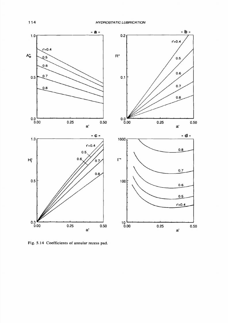
8/9/2019 Hydrostatic Lubrication 1992
http://slidepdf.com/reader/full/hydrostatic-lubrication-1992 131/558
114
HYDROSTATIC
LUBRICAT/ON
0.0
' '
0.00
0.25
0.50
a'
- c -
1.01
0.
R'
0
0
0.25 0.50
a'
- d -
a'
Fig. 5.14 Coefficients of annular recess pad.
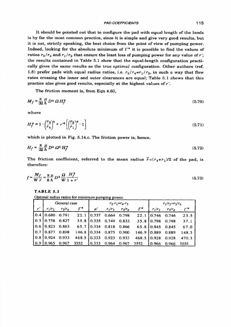
8/9/2019 Hydrostatic Lubrication 1992
http://slidepdf.com/reader/full/hydrostatic-lubrication-1992 132/558
PAD COEFFlClENTS 115
-
r'
0.4
0.5
0.6
0.7
0.8
0.9
It should be pointed out tha t to configure the pad with equal length of the lands
is
by
far
the most common practice, since it is simple and give very good results, but
it is not, strictly speaking, the best choice from the point of view of pumping power.
Indeed, looking for the absolute minimum of
r*
t
is
possible to find the values of
ratios r3Jr4 nd rl lr2 that ensure the least loss of pumping power for any value of r';
the results contained in Table 5.1 show that the equal-length configuration practi-
cally gives the same results as the true optimal configuration. Other authors (ref.
1.8) prefer pads with equal radius ratios, i.e.
r3/r4=r1/r2,
n such a way that flow
rates crossing the inner and outer clearances are equal; Table 5.1 shows that this
practice also gives good results, especially a t the highest values of
r'.
The friction moment is, from Eqn 4.60,
General case
rllr2 r3/r4 r*
0.680 0.791 22.1
0.758 0.827 35.8
0.823 0.863 65.7
0.877 0.898 146.8
0.924 0.933 468.5
0.965 0.967 3552
where
r2-rI=r4-r3
a'
rl /r2 r3/r4 r*
0.337 0.664 0.798 22.1
0.335 0.749 0.833 35 .8
0.334 0.818 0.866 65 .8
0.334 0.875 0.900 146.9
0.333 0.923 0.933 468.5
0.333 0.964 0.967 3552
which
is
plotted in Fig. 5.14.c. The friction power is, hence,
r1/r2=r3/r4
rl11-2 r3/r4 r*
0:746 0.746 23.5
0.798 0.798 37 .1
0.845 0.845 67 .0
0.889 0.889 148.3
0.928 0.928 470.3
0.966 0.966 3555
(5.70)
(5.71)
(5.72)
The friction coefficient, referred t o the mean radius F=(r4+r1)/2f the pad, is
therefore:
(5.73)
8/9/2019 Hydrostatic Lubrication 1992
http://slidepdf.com/reader/full/hydrostatic-lubrication-1992 133/558
116 HYDROSTATIC LUBRICATION
Hydrostatic thrust bearings with annular recesses are frequently used, very
often coupled to hydrostatic journal bearings. When the turning velocity is not high,
pumping power is much greater than friction power; on the basis of the above re-
sults,
it
is
easy
t o
make certain elementary suggestions:
r' should be low. In practice, due t o design constraints, we almost always
find that
r 5 0 . 5 .
Values greater than r'=0.8 should be avoided;
a'
should be in the
0.2+0.4
range;
D, i.e. the bearing area, should be as large as is allowed by the other design
constraints;
The film thickness
h
should be
low;
The lubricant viscosity
p
should be high.
EXAMPLE 5.5
An annular recess bearing must sustain a load W=20 KN, rotating at n=2n
radls (60 rpm); its outer diameter is D=O.l m, the inner one is 2rI=0.04 m (i.e.
r'=0.4). For clearance h=50 pm is chosen, and for a' the near-optimal value a'=l/3.
The lubricant data at T=40OC are:p=O.l Nslmz, p=9ooKglm3, ~ 1 9 0 0lKgSC.
From Eqn 5.66 we get A,=4.40.10-3 m2 and hence a recess pressure pr=4.55
MPa is needed to sustain the load. The hydraulic resistance of the pad (Eqn 5.68) is
R=22O,lO9
Nslm5
nd the flow rate proves to be Q=20.7.10-6m31s. The pumping
power is Hi=94 W. For friction we f ind: MfzO.0857 Nm, Hf=0.54 W, f=O.l22.lO-3,
respectively. The temperature step of the lubricant, from the inlet to the outlet of the
pad, is (Eqn 5.7) AT=2.7%, which is practically negligible.
Comparing these results to those already obtained for a circular recess pad with
the same diameter (Example 5.1), it may be noted that the friction of the annular
recess pad is lower; slightly greater pressure is required, but the flow rate and
power consumption are more than 4.5 times greater.
EXAMPLE 5.6
Let us change the inner radius of the bearing in the former example to rI=0.03
m (i.e. r'=0.6), and the angular speed to R=4n rad ls (120 rpm). We obtain p,=5.97
MPa, Q=46.8.10-6m3/s , Hi=279 W, Mf=0.147 Nm, Hf=1.85
W,
f=0.18.10-3,AT=3.5oC.
In comparison with the former example, a small increase in pressure may
again be noted, while for flow rate and pumping power the increase is much larger.
EXAMPLE 5.7
I f the inner radius is again increased to rl=0.04 m,
r'
becomes
0.8;
et the angu-
lar speed now be Q=6n rad ls (180 rpm). We find: pr=10.6 MPa, Q=187.10-6 m 3 / s ,
Hi=1989 W, Mf=0.146 Nm, Hf=2.76 W, f=0.16.10-3 and AT=6.2 C. Temperature in -
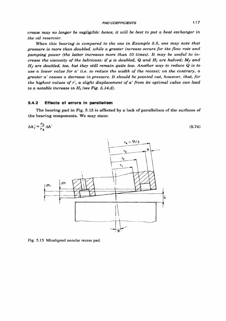
8/9/2019 Hydrostatic Lubrication 1992
http://slidepdf.com/reader/full/hydrostatic-lubrication-1992 134/558
PAD
COEFFlClENTS 117
crease may no longer be negligible: hence, it will be best to p u t a heat exchanger
in
the oil reservoir.
When this bearing is compared to the one in Example 5.5, one may note that
pressure
is
more th an dou bled, while a greater increase occurs fo r the flow rate an d
pumping power (the latter increases more than 10 t imes). It may be useful to in-
crease the viscosity of the lubricant: if p is doubled, Q and Hi are halved;
Mf
nd
H f are doubled,
too,
but they still remain quite low. Another way to reduce
Q
is to
use a lower value for a' (i.e. to reduce the w idt h of the recess); on th e contrary, a
greater a' causes a decrease in pressure. It should be pointed out , however, tha t, fo r
the highest values of
r',
a slight displacement of
a'
fro m its optimal value ca n lead
to a notable increase in Hi (see Fig. 5 .14.d).
5.4.2 Effec ts o f
errors i n
parallelism
The bearing pad
in
Fig. 5.15 is affected by a lack
of
parallelism
of
the surfaces of
the bearing components. We may state:
a h ; = % & * (5.74)
r4
Fig. 5.15
Misaligned
annular
recess
pad.

8/9/2019 Hydrostatic Lubrication 1992
http://slidepdf.com/reader/full/hydrostatic-lubrication-1992 135/558
118
HYDROSTATIC LUBRICATION
1
oo
0.95
CR
0.90
r'=0.4
0.6
0.8
0.85
0.0 0.5 1 o
Ah'
Fig. 5.16 Misaligned annular recess pad: correction factor
C,
versus parallelism error
Ah'
for two
values
of the land width ratio a'.
where
Ah'
is given by Eqn
5.31.
Bearing the results of section
5.3.3
in mind, we find
that, for a certain recess pressure
p r
and mean film thickness E , the only conspicu-
ous effect of misalignment is an increase in
flow
rate; such an increase may be
expressed as l/CR(Ah';
3 / r 4 )
or the external gap, and 1/cR(Ahi;
l / r z )
or the inter-
nal one. Thus, while the effective area
A,
may be considered to be practically unaf-
fected by a misalignment Ah'<1, the hydraulic resistance R may be expressed in the
form of Eqn 5.34; the correction factor
CR,
calculated as above, is plotted in Fig. 5.16
as a function of
Ah',
for certain values of r' and a'.
5.4.3
Effects
o f
pressure losses
at
the inlet
When the Reynolds number is greater than 100, the pressure losses at the inlet
should be taken into account. Applying the results of section 5.3.4 to both the gaps in
the annular recess pad, the whole hydraulic resistance of the pad should be cor-
rected as in Eqn
5.36,
where C p is given approximately by Eqn
5.39
(or by Fig.
5.61,
but the Reynolds number is
(5.75)
and
r ' ,
r
and A r must be substituted by the following:

8/9/2019 Hydrostatic Lubrication 1992
http://slidepdf.com/reader/full/hydrostatic-lubrication-1992 136/558
PAD
COEFFICIENTS
119
-
r =
rl
+
r2
+
r3
+
r4
4
r2 rl + r4
-
r3
2
r
=
EXAMPLE 5.8
A pad bearing with an annular recess has
an
outer diameter D=O.l m; the
inner one is 2rI=0.08 m (r'=0.8).It has to sustain a load W=15 KN, with
a
recess
pressure pr lower than
8
MPa. The angular speed is Q=6.28 radls (60 rpm); the
main characteristics of the lubricant are:
p=0.03
Nslm2,
885
e l m 3 .
Let us select a'=0.3; h=100 pm. We immediately find A,=1.98.10-3 m2 and,
hence, pr=7.58 MPa, which is safely smaller than the maximum pressure allowed.
If the pressure losses at the inlet are disregarded, we also find R=1.91.109 Nslm5,
and Q=3.97.1
0-3
3I s.
From the above equations, we find Re=207, F'=0.935,
r=0.045
m, Ar=3 mm. A
correction factor Cp=1.28 can be obtained from Fig.
5.6.
Since the flow rate is in-
versely proportional to the hydraulic resistance, a new value is found: Q=3.10.10-3
ma ts , which is still very high. On the other hand, the friction power is very small,
compared to the pumping power (Hf=O.O4
W,
is23.5 Kw). I f such a low friction is
not a design constraint, it is clearly advisable to reduce the selected clearance and to
increase lubricant viscosity, in order to greatly reduce flow rate and pumping
power.
5.4.4
Turbulent
f low
When the Reynolds number
is
high, the
flow
becomes turbulent. The results
already obtained in section 5.3.5 can be extended
t o
the annular recess pad. In par-
ticular, since in most cases both
r l l r 2
and
r31r4
are greater than 0.8, the influence
on the effective bearing area can be disregarded. The hydraulic resistance of the
pad, on the other hand, can now be written as:
(5.76)
Correction coefficient C R ~s still given by Eqn
5.48
(also plotted in Fig.
5.7.b)
n
which parameter
zb
is now defined as follows:
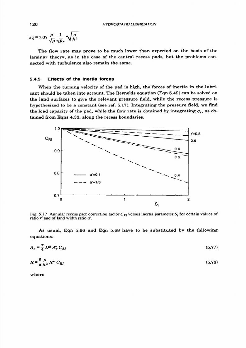
8/9/2019 Hydrostatic Lubrication 1992
http://slidepdf.com/reader/full/hydrostatic-lubrication-1992 137/558
120
HYDROSTATIC LUBRICATION
The flow rate may prove to be much lower than expected on the basis of the
laminar theory, as in the case of the central recess pads, but the problems con-
nected with turbulence also remain the same.
5.4.5
Effects of the iner t ia forces
When the turning velocity of the pad is high, the forces of inertia in the lubri-
cant should be taken into account. The Reynolds equation (Eqn 5.49) can be solved on
the land surfaces to give the relevant pressure field, while the recess pressure is
hypothesized to be a constant (see ref.
5.17).
ntegrating the pressure field, we find
the load capacity of the pad, while the flow rate
is
obtained by integrating qr, as ob-
tained from Eqns
4.33,
along the recess boundaries.
Fig. 5.17 Annular recess pad: correction factorCR, ersus inertia parameterSi for certain values of
ratio
r'
and
of
land width ratio
a'.
As usual, Eqn 5.66 and Eqn 5.68 have to be substituted by the following
equations:
(5.77)
(5.78)
where
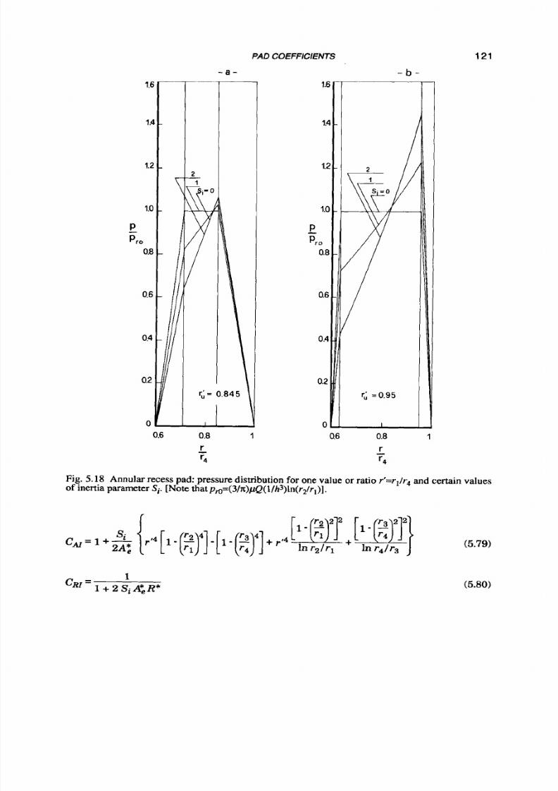
8/9/2019 Hydrostatic Lubrication 1992
http://slidepdf.com/reader/full/hydrostatic-lubrication-1992 138/558
PAD
COEFFICIENTS
121
- a -
- b -
I.€
1.1
1.2
1.0
P
Pro
-
0.8
0.6
0.4
0.2
0
0.6
2
-
1
-
SI'O
~
11
I?
1.:
1c
P
Pro
a8
0.6
0.4
0.2
0
r =0.95
0.8
1
0.6
0.8 1
r
r
-
'4
r4
Fig.
5.18
Annular reces s pad: pressure distribution for one value or ratio r'=r1/r4nd certain
values
of inertia parameterS,. Note thatpm=(3/7r)pQ( /h3)ln(r2/r,)].
(5.80)

8/9/2019 Hydrostatic Lubrication 1992
http://slidepdf.com/reader/full/hydrostatic-lubrication-1992 139/558
122
HYDROSTATIC LUBRICATION
For the correction factor CAI,however, we always have 0.99<CA1<1 for the most
common range of pad parameters: r50.5 , a'<0.3, Si<l . The correction factor CRI s
plotted in Fig. 5.17. From this diagram, it is clear that the effect of the iner tia forces
is
negligible, except for the lowest values of
r'
(consider, moreover, that
Si=l
is
a
high value). The friction parameters are not affected by the inertia forces.
I t should be pointed out that the pressure variations in the recess a re not always
negligible. In Fig. 5.18 (ref. 5.18) the pressure in the pad is plotted a s a function of
the radius, for two pads directly supplied a t constant flow, in the case
of
r'=0.6 and
r,Jr2=r3/r4=0.845and in the case of r'=0.6 and r11r2=r3/r4=0.95. nertia effects pro-
duce considerable differences in pressure a t the edges of the recess. I t is clear that
the hypothesis
of
constant recess pressure is not adequate. Nevertheless, when W
and
Q
have
to
be evaluated, the above results prove
to
be accurate enough.
ExluMPLE 5.9
An annular recess thrust bearing with D=O.l m and rI=0.03 m (thus r'=0.6)
sustains a load W=12KN and rotates at Lk200n radl s
(6000
pm); the lubricant data
are (at T=4OoC) =0.05 Nslm2, p=890 Qlm3, c=1920J I Q " C . Let us choose a'=0.25
and h=100pm.
If we disregard the turning velocity, we easily find a recess pressure pr=3.18
MPa and
a
flow rate Q=533.10-6m31s. We have Si=0.041, thus from Eqn 5.79 and Eqn
5.80, it is easy to verifv that the effect of
Si
is, in this case, totally negligible.
The pumping power is Hi=1695 W; the friction parameters are Mf=1.40 Nm,
Hf=881 W, and f=0.0029; this last value is comparable with that of the rolling bear-
ings at this speed.
The temperature increase is, in the case of adiabatic flow, about 2.8 c, and may
be disregarded.
EXAMPLE 5.10
Let
us now consider a bearing sustaining a load W=2
K N
at a=600nra dls (i.e.
18000 rpm, a value which cannot be reached by usual rolling bearings). We have
D=0.06 m, rl=0.02 m (r '=2/3),a'=0.25, h=50pm. The characteristics of the lubricant
are p=O.Ol Nslm2, p==70IQlm3, andc=1930JlK&"C,at T=40 C.
The recess pressure for Si=O is p,=1.70 MPa, and hence Si=0.246. It is easily
established that the effect of the turning velocity is still negligible on pr and Q. The
flow rate proves to be Q=O.222.lO-3m3/ s, and
the
pumping power Hi=377 W. The
friction power is Hf=373 W, and f=0.0040. The increase in temperature is about
2.0 C. The Reynolds number in outer clearance is Reu=205 see Eqn 5.59), and hence
the
flow is still laminar.
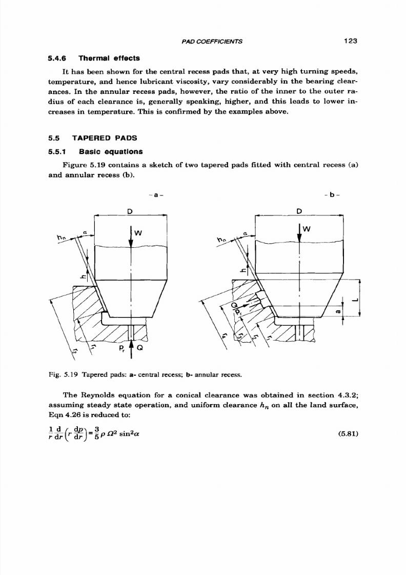
8/9/2019 Hydrostatic Lubrication 1992
http://slidepdf.com/reader/full/hydrostatic-lubrication-1992 140/558
PAD COEFFICIENTS 123
5.4.6 Thermal effects
It has been shown for the central recess pads that , a t very high turning speeds,
temperature, and hence lubricant viscosity, vary considerably in the bearing clear-
ances. In the annular recess pads, however, the ratio of the inner t o the outer ra-
dius of each clearance is, generally speaking, higher, and this leads
t o
lower in-
creases in temperature. This is confirmed by the examples above.
5.5
TAPERED PADS
5.5.1
Basic equat ions
Figure 5.19 contains a sketch of two tapered pads fitted with central recess (a)
and annular recess (b).
- a - - b -
*
Fig. 5.19 Tapered pads: a- central recess; b-
nnular
recess.
The Reynolds equation for a conical clearance was obtained in section 4.3.2;
assuming steady sta te operation] and uniform clearance h , on all the land surface,
Eqn
4.26
is reduced to:
(5.81)
8/9/2019 Hydrostatic Lubrication 1992
http://slidepdf.com/reader/full/hydrostatic-lubrication-1992 141/558
124 HYDROSTATIC LUBRICATION
The term on the right-hand side accounts for the inertia forces due to angular veloc-
ity0 n the simplest case, it i s negligible, and hence Eqn 5.81 is reduced to Eqn 4.56,
which does not depend on the aperture angle
a;
thus the pattern of the pressure
field
is
exactly the same
as
for a plane clearance
( a = d 2 )
of identical radius ratio
r'.
Stating pr=l ,and integrating p.sina on the recess and land surfaces, we obtain
the effective area
of
the pad. Again it turns out
to
be the same as for the plane bear-
ings, i.e. Eqn
5.20,
where A: is given by Eqn 5.22,or Fig. 5.l.b, for
the
central recess
pad, and by Eqn 5.67, or Fig. 5.14, for the annular recess pad.
The flow ra te a t radius r is obtained by integration of the radial velocity:
(5.82)
Let us disregard velocity R for the time being. The hydraulic resistance of the ta-
pered pads may be written as follows:
(5 .83)
where R* is given by Eqn 5.23 o r Fig. 5.l.b, and by Eqn
5.69
or Fig. 5.14, respectively.
It follows that the flow rate through a conical clearance will turn out to be propor-
tional
to
sina. The moment of the friction forces for an axial-symmetric conical land
of length dr is
C r Q
dMf = 2 x- r3 sin3a dr
hn
which may be easily integrated to give the friction moment:
and the friction power:
(5.84)
(5.85)
HF is exactly the same as that already calculated for the plane bearings: i.e. Eqn
5.28 for the central recess pad, and Eqn 5.71 for the other.
When
a
tapered pad is compared to a plane bearing of the same diameter, with
equal values of the normal film thickness and the same radius ratios, it is easy to
see that:

8/9/2019 Hydrostatic Lubrication 1992
http://slidepdf.com/reader/full/hydrostatic-lubrication-1992 142/558
PAD
COEFFICIENTS
125
the load capacity for any given recess pressure is the same (or ,
for
an equal
flow rate, is greater for the conical pads: actually, it is proportional t o
llsina);
the flow rate, a t any given load, is proportional t o sinq i.e. i t is lower for the
conical pads. The same Consequently, the same occurs for the pumping
power;
on the other hand the axial stiffness, which proves t o be inversely propor-
tional t o h=h,lsina, for any given load capacity, is lower (proportional to
sina) for the conical pads;
the friction power (proportional to llsina) is greater for the conical pads.
Furthermore, tapered pads have a greater axial size than the plane pads and
may prove to be more sensitive t o assembling misalignments.
EXAMPLE 5.11
An
annular recess tapered bearing has to sustain a load W=20KN, rotating at
Q=4a radls (120 rpm). The main geometrical parameters are: D=O.l m; L=0.02 m,
a=45'(i.e. rt=l-(2Ltga)lD=0.6).The viscosity of the lubricant is p=O.l N slmz at oper-
ating temperature.
I f
we select a'=113 and hn=50 pm
(or
h=70.7 pm), we easily obtain A50.427,
A,=3.35.103 m2, and hence p,=5.97 MPa; moreover, R*=O.0835, R=180.109 Nslm5,
and hence &=33.10-6 m3/ s . The pumping power is thus Hi=197 W. The friction
moment is easily calculated as Mf=0.208 Nm, while Hf=2.6 W. ompare these re-
sults with those in Example 5.6.
5.5.2
Effect of the inertia forces
As has been pointed out before, when Q is large, the inertia term should be re-
tained in Eqn
5.81.
This kind of problem is examined in ref.
5.17
for
the annular
recess pad, and i n ref. 5.19 for the central recess pad. In the latter, thermal effects
are also considered, as in ref. 5.13.
If we solve Eqn 5.81, and integrate the pressure field, we finally find that the
effective area
A,
is again given by Eqn
5.53
and Eqn
5.77
for the circular-recess and
the annular-recess pads, respectively.
In the same way, the hydraulic resistance will be:
(5.86)
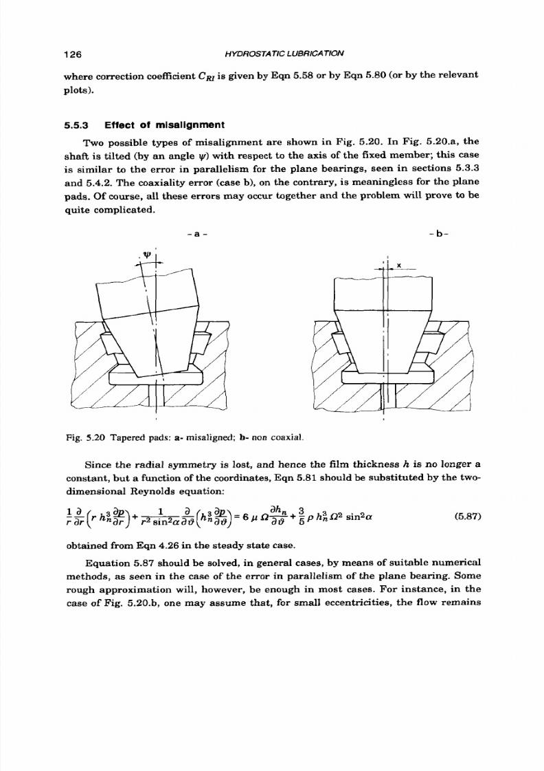
8/9/2019 Hydrostatic Lubrication 1992
http://slidepdf.com/reader/full/hydrostatic-lubrication-1992 143/558

8/9/2019 Hydrostatic Lubrication 1992
http://slidepdf.com/reader/full/hydrostatic-lubrication-1992 144/558
PAD
COEFFlClENTS 127
essentially radial. In this assumption, the effective area does not vary; the flow rate
on a sector dfi of the conical surface is (see Fig.
4.5):
The clearance may be written in the following form:
h ,
=
C
o s a 1
cos
( 1 9- @]
[ "
where C&tga is the mean radial play. The flow rate is, hence:
x
x 3
21r
Q =
J d Q = G z p r sin4a(l+t$)
0
Thus correction factor C R x
for
the hydraulic resistance can be evaluated as:
(5.89)
Friction is also affected by a radial displacement x . Proceeding as above, we can
assess a correction factor
Cfxfor
M f
and
Hf,
hich may be written as:
1.21
1.1
-
1
o
0.9
0.8
-
0.7
-..
0.0 0.1 0.2 0.3 0.4 0.5
X/C
Fig. 5.21 Non coaxial tapered pad: correction factors
C R ~
or the hydraulic resistance and Cfx
for
friction versus radial displacement
xlC.

8/9/2019 Hydrostatic Lubrication 1992
http://slidepdf.com/reader/full/hydrostatic-lubrication-1992 145/558
128
Cfr
=
1
<
HYDROSTATIC LUBRICATION
(5.90)
It is clear tha t a radial displacement, comparable to the design value of the film
thickness, greatly affects the hydraulic resistance of the pad, and consequently the
performance of the bearing. This point should be carefully considered when design-
ing. For example, if a conical thrust bearing sustains a shaft which is also loaded
in a radial direction, the stiffness of the radial bearings will interact with the axial
load capacity.
The case of Fig. 5.20.a (tilting error) is examined in ref. 5.20 by means of numer-
ical integration (finite differences) of Eqn
5.87.
The effect of a relative tilt
1y'=1yDl(2h,)10.6
on the hydraulic resistance
(at
low speed) is found to be always
smaller than for a flat bearing (a=90 ).n particular, it is negligible for
a=60 +75 ,
while a=45 is an intermediate case.
When the speed
is
high, the hydrodynamic effect, due to the uneven clearance,
may in part counterbalance the effect of the tilting error, and
a
tilted bearing may
even prove to perform better than
a
centered one
5.6
SPHERICAL
PADS
To overcome the problems connected with the tilting errors,
a
spheri-
cally-shaped pad (Fig. 5.22) could be used, instead of the flat or tapered types.
A s
usual, to calculate the performance of the pad, the relevant Reynolds equa-
tion must be solved to find the pressure in the clearances. Such an equation has
been obtained in section
4.3.3.
For an axial-symmetric spherical clearance, Eqn
4.30
is reduced to:
The above equation is easily solved when E=O (concentric configuration), giving:
Pr
tan (~112
In
(5.91)
for the central recess pad, with p=pr for p q l andp=O for p q 2 . A general solution
may however be obtained (ref.
5.21,
5.22), although the relevant equations are quite
cumbersome.
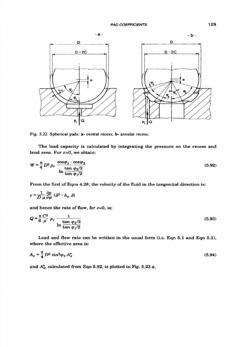
8/9/2019 Hydrostatic Lubrication 1992
http://slidepdf.com/reader/full/hydrostatic-lubrication-1992 146/558
PAD COEFFICIENTS
129
- a -
- b -
Fig. 5.22 Spherical pads: a- central recess; b- annular recess.
The load capacity is calculated by integrating the pressure on the recess and
land area.
For
E=O, we obtain:
(5.92)
From the first of Eqns 4.28; the velocity
of
the fluid in the tangential direction is:
u = -
* ( @ - h , @
D P a P
and hence the rate
of flow,
for
E=O,
is:
(5.93)
Load and flow
rate
can be written in the usual
form
(i.e. Eqn 5.1 and Eqn
5.21,
where the effective area is:
A,
=
x 0 2 sin2q2A*,
(5.94)
and A*,,calculated from Eqn 5.92, is plotted in Fig. 5.23.a.
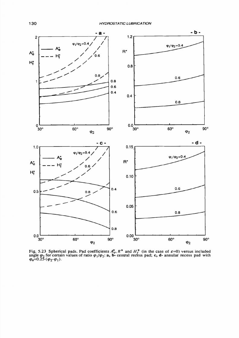
8/9/2019 Hydrostatic Lubrication 1992
http://slidepdf.com/reader/full/hydrostatic-lubrication-1992 147/558
130
2
A',
Hi
1
t
HYDROSTATIC LUBRICA
TlON
0.8
0.6
0.4
I"
60"
90"
(92
- c -
0.8
0.4
0.0
60" 90"
(92
30'
- d -
0 . 1 5 - 7
0.05
1
0.00' ' '
.
' . ' '
30"
60" 90"
(92
Fig. 5.23 Spherical pads. Pad coefficients
A*,,
R *
and
H,?
(in the case of
E=O)
versus included
angle (p2
for certain values of ratio (p1/(p2:
a, b-
central recess pad; c,
d-
annular recess pad with
(pa=O.25'((p2-(pl).
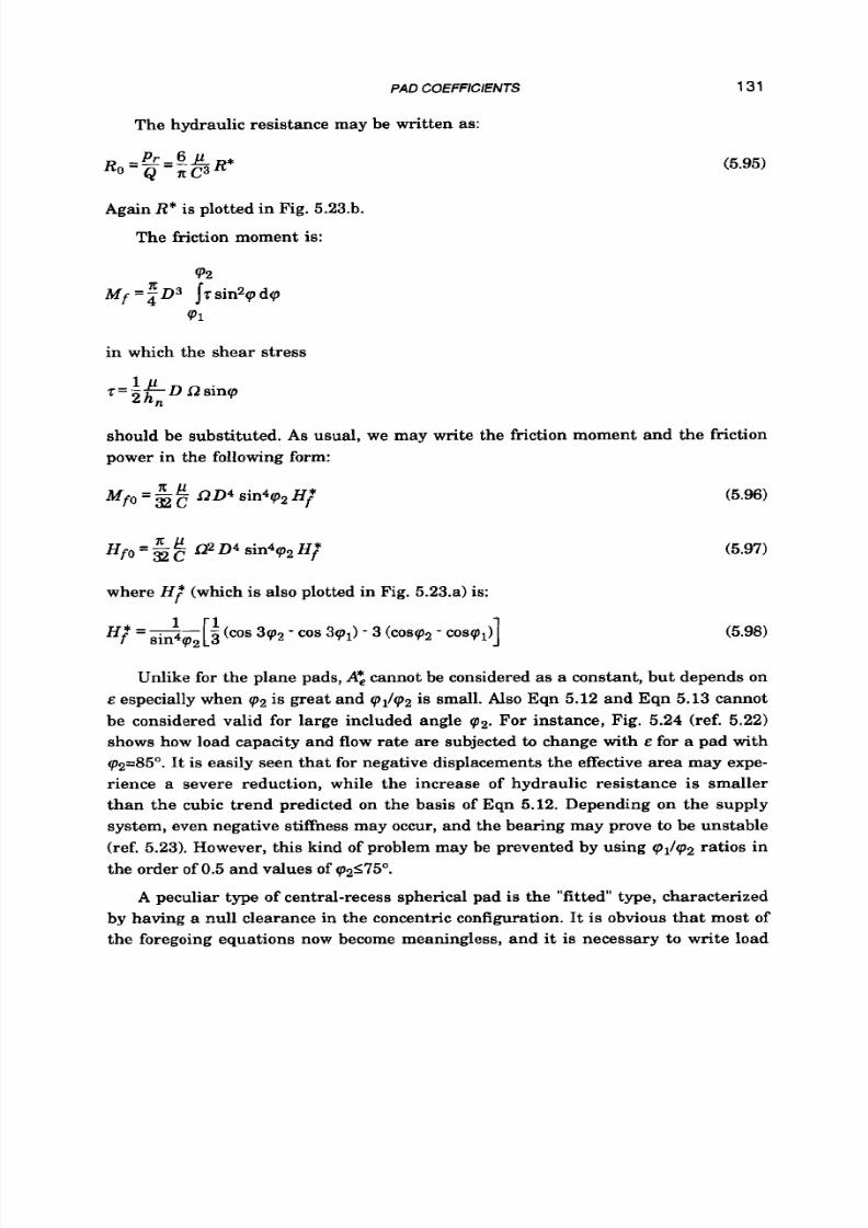
8/9/2019 Hydrostatic Lubrication 1992
http://slidepdf.com/reader/full/hydrostatic-lubrication-1992 148/558
PAD
COEFFlClENTS
131
The hydraulic resistance may be written as:
(5.95)
Again R* is plotted in Fig. 5.23.b.
The friction moment is:
in which the shear stress
should be substituted. As usual, we may write the friction moment and the friction
power in the following form:
M f o =
2
$
f2 4
in4q2H,F
(5.96)
where HT (which is also plotted in Fig. 5.23.a) is:
(5.98)
Unlike for the plane pads, A*,cannot be considered as a constant] bu t depends on
E especially when
cp2 is
great and q1/cp2 is small.
Also
Eqn 5.12 and Eqn 5.13 cannot
be considered valid for large included angle q2. For instance] Fig. 5.24 (ref.
5.22)
shows how load capacity and flow rate are subjected
to
change with E for a pad with
cp2=85". It is easily seen tha t for negative displacements the effective area may expe-
rience a severe reduction] while the increase of hydraulic resistance is smaller
than the cubic trend predicted on the basis of Eqn 5.12. Depending on the supply
system, even negative stiffness may occur, and the bearing may prove to be unstable
(ref. 5.23). However, this kind of problem may be prevented by using q1/q2 ratios in
the order of 0.5 and values of q2S75".
A peculiar type of central-recess spherical pad is the "fi tted' type, characterized
by having a null clearance in the concentric configuration.
It
is obvious that most of
the foregoing equations now become meaningless, and it is necessary to write load

8/9/2019 Hydrostatic Lubrication 1992
http://slidepdf.com/reader/full/hydrostatic-lubrication-1992 149/558
132
1.0
0.8
w
2
.6
0
2
n
a
5 0.4
0.2
0
HYDROSTATIC LUBRICATION
- a -
-
b -
0.2
0.4
0.6
a8 t o
?
1
0 0.2 0.4 0.6 0.8
4 ’%
Fig. 5.24 Sphe rical pad with cenh-a1 recess: a- load factor W.4/(zDzprsin&p) and b-
flow
factor
Q-pl[(l+~)%?p,]
ersus ratio q1/(p2or a number of values
of
eccentricity
E
(ref.
5.22).
capacity and flow rate as functions of the displacement h=h,(cp=O). We obtain (ref.
5.24):
x tan2q2 - tan2cpl
W
=4 D2
p r
tan 472
tan2472
-
tan2ql + 2 In-
tan
471
& = - -
h3 p
1
tan472
tan2472
-
tan2cpl + 2 In
tan471
3 P
Torque is found to be (ref. 5.21)
Mr g f
RD4 ( ~ 0 ~ 2 4 7 ~cos2ql -
2
ln-
Spherical bearings have also been studied from the point
of
view
of
the effects of
fluid inertia (ref.
5.21)
and of change in viscosity due
t o
adiabatic flow (ref. 5.25). It

8/9/2019 Hydrostatic Lubrication 1992
http://slidepdf.com/reader/full/hydrostatic-lubrication-1992 150/558
PAD
CO€FF/CENTS 133
has been shown that high values of the inertia parameter Si defined in Eqn
5.50
(perhaps Sp0.25) are detrimental for divergent film shapes, i.e. for negative eccen-
tricities: load capacity may be notably reduced, and even cavitation is likely
to
occur.
On the contrary, for converging film shapes (e.g. for the
fitted
type of bearing) load
capacity is improved and, due to the large pressures developed near the edge, bear-
ings with a wide included angle
(p2
also feature a notable radial load capacity.
The annular recess pads (Fig. 5.22.b) feature an effective area
W l p ,
that does not
vary much with eccentricity, especially when cp z is small. Proceeding
as
above, we
can calculate the relevant values of parameters A:
R*
and HF
to
be inserted in the
equations from Eqn 5.94 to Eqn 5.97. They are plotted in Fig. 5.23.c and Fig. 5.23.d.
For
A*,it
may be taken approximately (see also ref. 5.26):
(5.99)
at least when (pa is smaller than 0.25((p2-cpl).
5.7 RECTANGULAR
PADS
For a rectangular pad, such as in Fig. 5.25, the two-dimensional Reynolds equa-
tion Eqn 4.15 has to be solved, which, if h=const or
U=O,
is
simply reduced to Eqn
4.31 (Laplace equation). The boundary conditions are, as usual,
p = p r
at the inner
boundary of the clearance, and p=O
at
the outer one. Once the pressure on the land
area has been evaluated, the load capacity
is
obtained by integration. The rate of
flow, on the other hand, is given by the following:
(5.100)
where
S
is the inner boundary
( o r
any closed contour including it), and
n
is
the
outer normal direction of
S
(see also section 4.5.2).
In spite of
its
simplicity, Eqn 4.31 may be solved, in the general case, only by
numerical methods.
A first
rough approximation can be very easily obtained by
partitioning the land area as in Fig. 5.26 (ref.
1.8).
The pressure
is
assumed
to
vary
with a linear trend (see section 4.7.1) along the
.z coordinate, for parts [ l l and 121,
and along z for parts
131
and [41. In the corners, a logarithmic trend is assumed (see
section 4.7.4); if we have ri=O, the corners may be neglected altogether.
Calculations for load and flow rate are now straightforward: on the analogy
with the other pad types, the effective area
A,
and the hydraulic resistance R may be
written as:

8/9/2019 Hydrostatic Lubrication 1992
http://slidepdf.com/reader/full/hydrostatic-lubrication-1992 151/558
134
HYDROSTATIC LUBRICATION
4
J
Fig. 5.25 Rectangular pad.
A , =
L B
A
R=$R*
with
a ' l B ' +
2
rib'
In l+-
a'
4 ri 6'
(a'
+ r ib'
B')
+
Za'
( r i b
B )
R*
= 6
n:
In
( +-
r l E ' B )
where
(5.101)
(5.102)
(5.103)
(5.104)
a'
-a b
B ' = -
ri
and
q'=Z
- L ; b ' = B ;
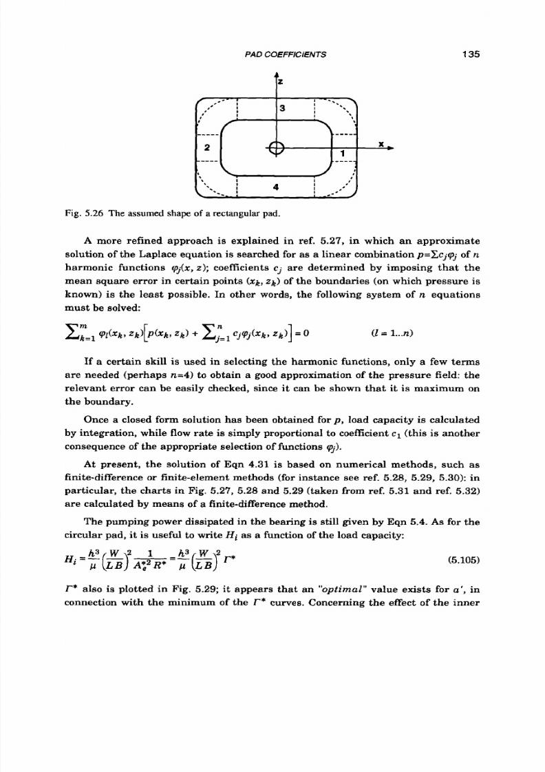
8/9/2019 Hydrostatic Lubrication 1992
http://slidepdf.com/reader/full/hydrostatic-lubrication-1992 152/558
PAD
COEFFlClENTS
135
Fig.
5.26 The assumed shape of
a
rectangular pad.
A
more refined approach
is
explained in ref. 5.27, in which an approximate
solution of the Laplace equation is searched for as a linear combinationp=Xc jq j of n
harmonic functions qJx, z ) ; coefficients
cj
are determined by imposing that the
mean square error in certain points
( x k ,
Zk) of the boundaries (on which pressure
is
known) is the least possible. In other words, the following system of n equations
must be solved
If a certain skill
is
used in selecting the harmonic functions, only a few terms
are needed (perhaps n=4) to obtain a good approximation of the pressure field: the
relevant error can be easily checked, since it can be shown that it is maximum on
the boundary.
Once a closed form solution has been obtained forp , load capacity is calculated
by integration, while flow rate
is
simply proportional to coefficientc 1 (this is another
consequence of the appropriate selection of functions
9).
A t present, the solution of Eqn 4.31 is based on numerical methods, such as
finite-difference or finite-element methods (for instance see ref. 5.28, 5.29, 5.30): in
particular, the charts in Fig. 5.27, 5.28 and 5.29 (taken from ref. 5.31 and ref. 5.32)
are calculated by means of a finite-difference method.
The pumping power dissipated in the bearing is still given by Eqn5.4. As for the
circular pad, it is useful to write
Hi
as a function of the load capacity:
(5.105)
r*also is plotted in Fig. 5.29; it appears that an “opt imal”value exists for
a‘,
n
connection with the minimum of the r*curves. Concerning the effect of the inner

8/9/2019 Hydrostatic Lubrication 1992
http://slidepdf.com/reader/full/hydrostatic-lubrication-1992 153/558
136 HYDROSTATIC LUBRICATlON
3
R'
2 -
1
0
- a -
F]
.
0.5
0.25
0.
0.
0.0
0.2 0.4
a'
- b -
0.3'
. ' ' ' . . '
0.0
0.1
a'
Fig. 5.27 Rectangular pads: pad coefficient
keversus
land width a'.
0.2
- b -
1.5
1 o
0.5
0.5
0.0
0.1 0.2
a'
Fig. 5.28 Rectangular pads: pad coefficient
R*
versus
land width a'.
fillet radius ri, although this yields a lower load capacity,
it
appears to be effective
from the point
of
view of power. On the contrary, the outer radius
r,,
which is not
considered in the charts above, has negative effects on both A,
and H i , and should
be avoided (however, when r,+r,lBs0.25, it has no practical influence on the per-
formance of the pad).
The friction force on the pad, due
to
a
sliding velocity
U,
s (from
Eqn
4.35):
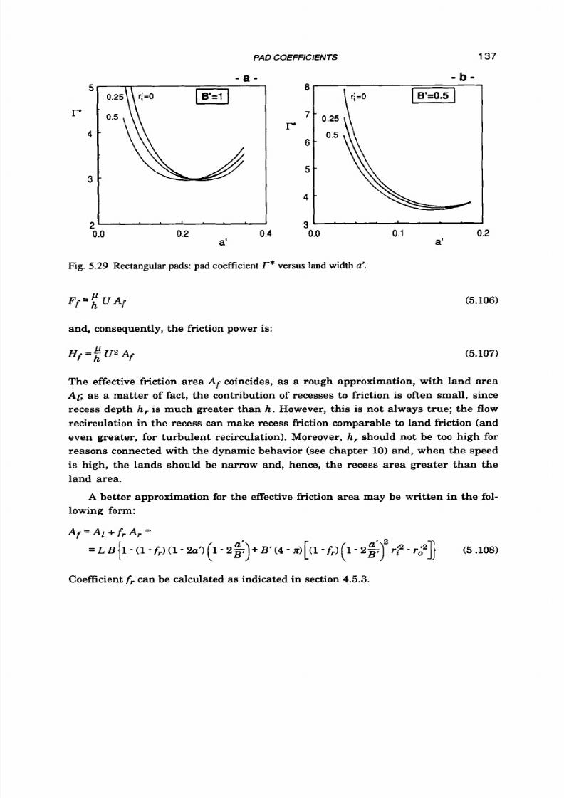
8/9/2019 Hydrostatic Lubrication 1992
http://slidepdf.com/reader/full/hydrostatic-lubrication-1992 154/558
PAD
COEFFICIENTS 137
r
r
- b -
8
0.25
0.5
6 -
5 -
4 -
.J
0
o
0.1
0.2
a'
Fig. 5.29 Rectangular pads: pad coefficient r*
ersus
land width
a'.
(5.106)
and, consequently, the friction power is:
The effective friction area
A f
coincides, as a rough approximation, with land area
Al;
as a matter of fact, the contribution of recesses
to
friction is often small, since
recess depth h, is much greater than h. However, this is not always true; the
flow
recirculation in the recess can make recess friction comparable to land friction (and
even greater,
for
turbulent recirculation). Moreover, h, should not be too high for
reasons connected with the dynamic behavior (see chapter 10) and, when the speed
is high, the lands should be narrow and, hence, the recess area greater than the
land area.
A better approximation
for
the effective friction area may be written in the fol-
lowing form:
A t = Al
-I-,
A , =
= L € ? { l - ( l - f , ) ( l - 2 ~ ' ) + B ' ( 4 - d [ ( l - f r ) ( 1 - 2 8 ; )'
2 r i 2 - r i 2 ] ]
(5.108)
Coefficient f, can be calculated as indicated in section 4.5.3.
8/9/2019 Hydrostatic Lubrication 1992
http://slidepdf.com/reader/full/hydrostatic-lubrication-1992 155/558
138 HYDROSTA TIC LUBRICA TlON
EXAMPLE 5.12
A rectangular pad has to be designed, able to carry a 45 KN load. The width of
the pad should be B=O.I m; the recess pressure should be lower than 4 MPa and the
friction coefficient lower than 10-4 at a speed U=0.2 mls . The viscosity of the lubri-
cant to be used is p=0.03 Nsl m2 .
Due to the constraint on pr, the effective area (Eqn 5.1) must be greater than
11.3.10-3 m2. Figure 5.27 shows that, for values of a’ near to the “optimal”,A: takes
on values greater than 0.55; consequently, we may take LB=0.02 m2, i.e. L=0.2 m
and B’=0.5. If
we
select a’=0.125 (i.e. b’=0.5) and ri=0.5, in Fig. 5.27 and Fig. 5.28 we
read Az=0.6, R*=0.77; hence A,=0.012
m2,
pr=3.75 MPa. The land area is easily cal-
culated as A1=0.013 m2; from Eqn 5.106 it follows that, for f d O - 4 , it must be h>17.3
pm: a very small value. A more suitable selection may be h=30
pm;
now Eqn 5.104
gives R=0.86.1012Nslm5 and hence &=4.4.10-6mats; the pumping power dissipated
in the bearing clearaAce is Hi=16.5 W . A more accurate calculation o f the effective
friction area (Eqn 5,108) gives, for hr=0.5 mm, Af=0.015 ma; the friction power is,
hence, Hf=O.6 W (Eqn 5.107) and the friction coefficient is f=0.67.lfY4. It should be
stressed that in th is case a relatively small recess has been selected since the speed
was quite low: indeed, the friction power turns out to be much smaller than the
pumping power. For higher speeds, a larger recess would have been a more suit-
able selection. This kind of problem, extensively dealt with in chapter 11, will also be
considered in section 6.4.
5.8
CYLINDRICAL PADS
Cylindrical pads may be used to support a shaft in a radial direction. They may
be thought of as extensions of any flat pad shape (e.g. the pad with a circular pro-
jected area in Fig. 5.30.a), although the rectangular shape is by far the most com-
mon (Fig. 5.30.b). It must be pointed out that a single-recess cylindrical pad is prac-
tically unable to sustain side loads; this greatly reduces the usefulness of such pads,
unless they are a part
of
a multipad bearing system (see section
7.5).
The study of these pads is made, as usual, by finding a solution for the relevant
Reynolds equation, i.e. of Eqn 4.18. n that equation, the right-hand side accounts
for the effects of the turning velocity of the journal and for the squeeze effect under
dynamic loading. Film thickness h depends on the displacement of the journal
center:
h = C [I- E C O S ( ~ - ~ ) ]
(5.109)
in which
C
s the film thickness in the concentric configuration
E=O
(see also Fig.
4.4).Once the pressure field on the pad lands is known, both the load capacity and
the rate of flow are easily evaluated, as in the preceding sections.
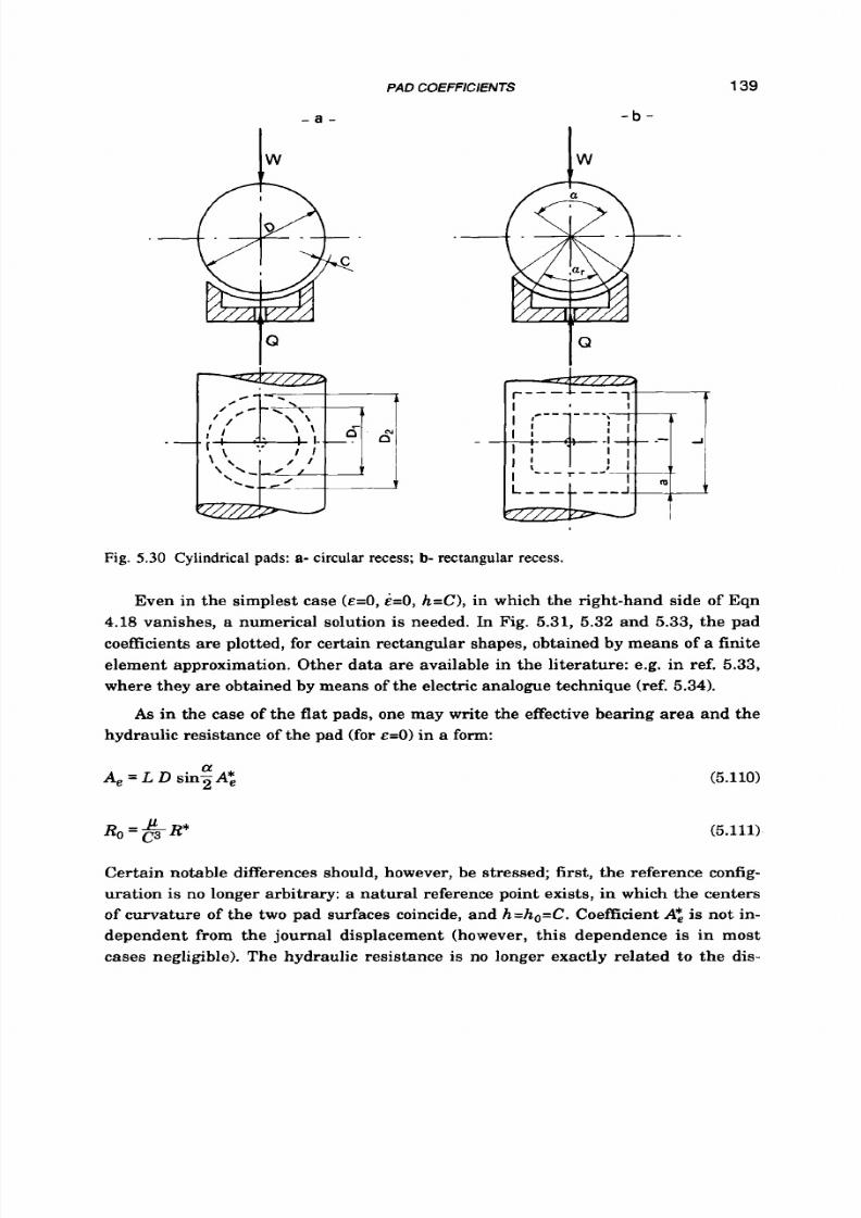
8/9/2019 Hydrostatic Lubrication 1992
http://slidepdf.com/reader/full/hydrostatic-lubrication-1992 156/558
I W
PAD COEFFICIENTS
- a -
139
- b -
l Q
.i
Q
Fig.
5.30
Cylindrical
pads: a-
circular
recess; b- rectangular recess.
Even in the simplest case (E=O,
&=O,
h = C) , in which the right-hand side of Eqn
4.18
vanishes, a numerical solution is needed. In Fig.
5.31, 5.32
and
5.33,
he pad
coefficients are plotted, for certain rectangular shapes, obtained by means
of
a finite
element approximation. Other data are available in the literature: e.g. in ref.
5.33,
where they are obtained by means
of
the electric analogue technique (ref.
5.34).
As
in the case of the flat pads, one may write the effective bearing area and the
hydraulic resistance of the pad (for E=O) in a form:
a
A,
=
L D sinTA*,
(5.110)
R ~ = & R *
(5.111)
Certain notable differences should, however, be stressed; first, the reference config
uration
is
no longer arbitrary: a natural reference point exists, in which the centers
of curvature
of
the
two
pad surfaces coincide, and
h=ho=C.
Coefficient
A*,
is not in-
dependent from the journal displacement (however, this dependence is in most
cases negligible). The hydraulic resistance is no longer exactly related
t o
the dis-
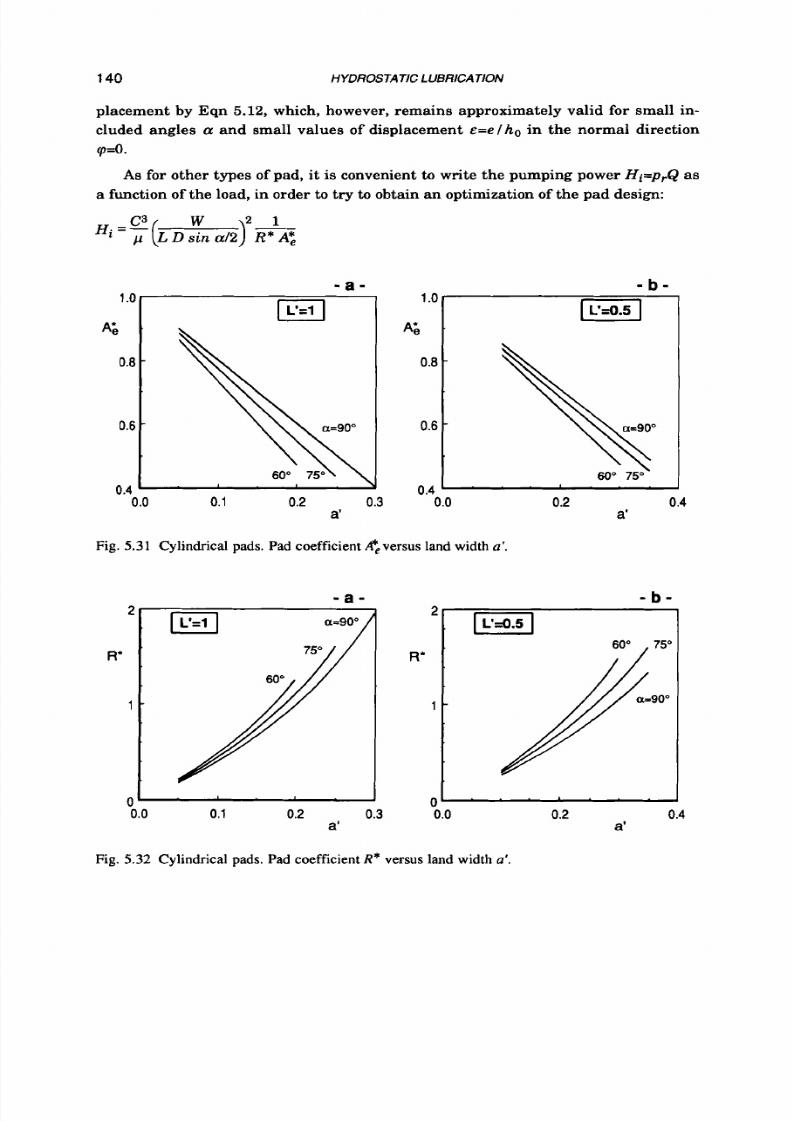
8/9/2019 Hydrostatic Lubrication 1992
http://slidepdf.com/reader/full/hydrostatic-lubrication-1992 157/558
140 HYDROSTATIC LUBRICATION
1.o
A ' , '
0.6
0.4
o . 8 #
placement by Eqn 5.12,which, however, remains approximately valid for small in-
cluded angles
a
an d small values of displacement E = e / h o n the normal direction
rp=O.
As for other types of pad, it is convenient to write th e pumping power Hi=p,Q as
a function of the load, in order to try to obtain an optimization of the pad design:
60"
75
\
- a - - b -
0.4' . ' ' ' . . '
0.0
0.2
0.4
a'
Fig. 5.31 Cylindrical pads. Pad coefficient Heversus land width a'.
- a -
R'
0.0 0.1 0.2 0.3
a'
a'
0.0 0.2 0.4
a'
Fig. 5.32 Cylindrical pads. Pad coefficientR* versus land width
a'.

8/9/2019 Hydrostatic Lubrication 1992
http://slidepdf.com/reader/full/hydrostatic-lubrication-1992 158/558
PAD COEFFICIENTS 141
In particular, given L,
D,
and a, he relevant "optimal" value of a ' may be readily
evaluated by means of the plots of T*=lfR*A*,n Fig. 5.33.
The friction moment, in the concentric configuration E=O, s:
The friction power is, consequently,
(5.112)
(5.113)
The effective area Af may be calculated as for rectangular pads; namely, as a rough
approximation,
Af
coincides with the developed land area; if instead the recess fric-
tion is also taken into account, Afmay be written as:
(5.114)
The friction factor
f ,
is evaluated as in section 4.7.3; owever, in most cases one may
simply take f,=4C/h,.
- a -
u=90"
2
0.0 0.1 0.2 0.3
a'
- b -
6 -
r*
4
t
2 '
0.0 0.2 0.4
a'
Fig.
5.33
Cylindrical pads. Pad coefficient r*versus land width a .
5.9
HYDROSTATIC
LIFTS
A particular application (ref. 1.5) of externally pressurized lubrication consists
in relieving large hydrodynamic bearings in certain critical operations, such as
starting or stopping, in which, due to insufficient velocity, the lubricant film would
be ruptured, leading
t o
high friction and fast wear. In certain applications, in

8/9/2019 Hydrostatic Lubrication 1992
http://slidepdf.com/reader/full/hydrostatic-lubrication-1992 159/558
142
HYDROSTATIC LUBRICATlON
which the torque available is not much greater than the normal regime torque,
starting can even prove t o be impossible without the aid of a hydrostatic lift. This
kind of bearings (Fig. 5.34) are often referred to as "hybrid" journal bearings; it
seems, however, more appropriate to define them as hydrodynamic bearings with a
hydrostatic lift, since external pressurization is generally confined to low speed
running, while it is removed during normal running.
)Wa-
Li
IQ
IQ
II
I - b -
lw
Fig. 5.34
Hydrostatic
lift:
a-
axial recess; b- circumferential recess.
Behavior of such a "hybrid" bearing (studied for instance in ref. 5.35-5.37) is
beyond the scope of a work on hydrostatic lubrication; we shall therefore present
results relevant to the hydrostatic lift alone.
Due to the large included angle (we may assume a=180°) and to the smallness of
the recess, Eqn 5.12 is clearly far from representing the actual increase of hydraulic
resistance with eccentricity, and even the effective area can no longer be considered
as
a
constant. In Table 5.2, values are reported of the nondimensional load capacity
for eccentricities from E=O &=0.8,assuming constant-flow direct supply, obtained
by means of a finite element program (ref. 5.38). Several sizes of recesses have been
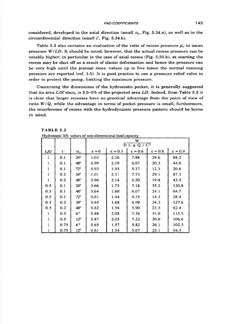
8/9/2019 Hydrostatic Lubrication 1992
http://slidepdf.com/reader/full/hydrostatic-lubrication-1992 160/558
PAD COEFFICIENTS 143
considered, developed in the axial direction (small a,,Fig. 5.34.a), as well as in the
circumferential direction (small
I ,
Fig. 5.34.b).
Table
5.3
also contains an evaluation of the ratio of recess pressure
p ,
t o mean
pressure W I L D . It should be noted, however, that the actual recess pressure can be
notably higher; in particular in the case of axial recess (Fig. 5.30.b), at starting the
recess may be shut
off as
a result of elastic deformation and hence the pressure can
be very high until the journal rises: values up to five times the normal running
pressure are reported (ref. 1.5). It is good practice t o use a pressure relief valve in
order to protect the pump, limiting the maximum pressure.
Concerning the dimensions of the hydrostatic pocket,
it
is generally suggested
that i ts area LDl'sina, is 2 .54% of the projected area LD. Indeed, from Table 5.3 it
is clear that larger recesses have no practical advantage from the point of view of
ratio
W/Q,
hile the advantage in terms
of
pocket pressure is small; furthermore,
the interference of recess with the hydrodynamic pressure pattern should be borne
in mind.
T A B L E 5.2
Iydro:
VD
1
1
1
1
1
0.5
0.5
0.5
0.5
0.5
1
1
1
1
-
-
tic lift:
-
1'
0.1
0.1
0.1
0.2
0.2
0.1
0.1
0.1
0.2
0.2
0.5
0.5
0.75
0.75
-
-
a
L
2 4 O
4 8 O
72"
24"
48"
24
48
72"
24"
48
6"
12O
6'
12"
-
on-dimensional load capacity.
W
D L p Q / C 3
E = O
~~
1.03
0.99
0.93
1.01
0.96
0.66
0.64
0.61
0.65
0.62
0.88
0.87
0.65
0.61
E
= 0.3
2.36
2.19
1.95
2.31
2.14
1.73
1.60
1.44
1.68
1.56
2.08
2.05
1.57
1.54
E =
0.6
7.88
6.67
5.17
7.73
6.50
7.18
6.07
4.74
6.98
5.90
7.34
7.22
5.82
5.67
E
=
0.8
29.6
20.3
12.3
29.1
19.8
35.2
24.1
14.3
34.3
23.3
31.0
30.0
26.1
25.1
E =0.9
88.2
44.6
20.6
87.3
43.5
130.8
64.7
28.4
127.6
62.4
115.5
106.6
102.3
94.3

8/9/2019 Hydrostatic Lubrication 1992
http://slidepdf.com/reader/full/hydrostatic-lubrication-1992 161/558
144
T A B L E
5.3
[ydrol
UD
1
1
1
1
1
0.5
0.5
0.5
0.5
0.5
1
1
1
I
-
-
itic lift:
1'
0.1
0.1
0.1
0.2
0.2
0.1
0.1
0.1
0.2
0.2
0.5
0.5
0.75
0.75
-
-
HYDROSTATIC
LUBRICATION
-o
non-dimensional
recess pressure.
a
24
48"
720
24"
48"
2 4 O
48"
720
Z"
48
6
12
6
12
-
E = O
3.38
2.73
2.36
2.97
2.42
3.97
2.95
2.41
3.55
2.65
2.76
2.56
2.40
2.23
E = 0.3
3.75
2.95
2.49
3.26
2.58
4.15
3.06
2.47
3.72
2.74
3.05
2.81
2.63
2.42
PI
W I D L
E
=
0.6
4.53
3.38
2.73
3.85
2.90
4.55
3.25
2.58
4.05
2.90
3.66
3.31
3.12
2.82
E = 0.8
5.85
4.02
3.06
4.81
3.34
5.21
3.52
2.7 1
4.55
3.11
4.72
4.13
3.92
3.43
E = 0.9
7.35
4.67
3.38
5.85
3.77
5.88
3.80
2.82
5.08
3.30
5.99
5.03
4.83
4.05
EXAMPLE 5.13
The following are the data of a hydrodynamic journal bearing: D=0.5 m, L=0.4
m, C=0.3 mm, W=300 N. The lubricant is a
SAE
30 oil (p=O.l Ns lm 2 at operating
temperature). Let us try to design
a
suitable hydrostatic lift.
First, one may establish the dimensions of the recess.
For
instance, we may
select
1=60
m m (i.e. l'=0.15) and a circumferential width b=100 m m (ar=23?. The
flow rate and pressure
o f
the pump can be calculated once the working eccentricity
has been selected. If
we
choose
&=0.8
corresponding to a minimum film thickness
h=60
pm), by interpolating data in the relevant column
of
Table
5.2,
he flow rate
turns out to be
Q=WC31(32~DLp)=0.013~103
31s. From Table 5.3 we may obtain a
recess pressure pr=Wl(0.19.LD)=7.9 MPa; as noted above, the l ifting pressure will be
much greater, and the value above should be considered as only a rough indication.
5.10 SCREW AND NUT ASSEMBLY
This particular kind of bearings (ref.
5.39),
shown in Fig. 5.35, is dealt with in
the usual way, i.e. by writing down the Reynolds equation in a suitable coordinate
system, and solving it for the pressure field. Then, to find the load capacity and the
rate of flow is straightforward: e.g. see ref.
5.40
and ref.
5.41.
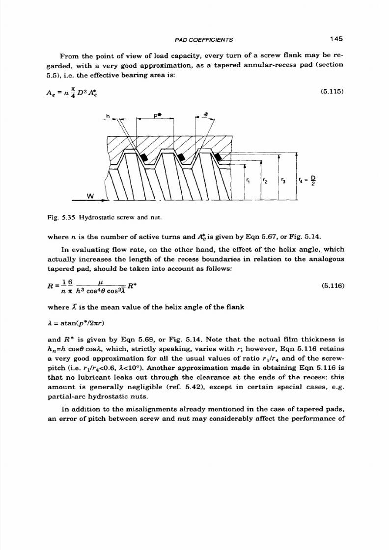
8/9/2019 Hydrostatic Lubrication 1992
http://slidepdf.com/reader/full/hydrostatic-lubrication-1992 162/558
PAD
COEFFlClENTS 145
From the point of view of load capacity, every turn of a screw flank may be re-
garded, with a very good approximation, as a tapered annular-recess pad (section
5.51, i.e. the effective bearing area
is:
x
A, =
n 4 2
A*,
(5.115)
Fig. 5.35 Hydrostatic screw and nut.
where n is the number of active turns and A*,is given by Eqn 5.67,or Fig. 5.14.
In evaluating flow rate, on the other hand, the effect of the helix angle, which
actually increases the length of the recess boundaries in relation
t o
the analogous
tapered pad, should be taken into account as follows:
(5.116)
where
is the mean value of the helix angle of the flank
2. = atan(p*/2xr)
and R* is given by Eqn 5.69, or Fig. 5.14. Note that the actual film thickness is
h,=h
cose cod , which, strictly speaking, varies with r; however, Eqn 5.116 retains
a very good approximation for all the usual values of ratio r l / r 4 and of the screw-
pitch (i.e. r1/r4<0.6, c l O ) . Another approximation made in obtaining Eqn 5.116 is
that no lubricant leaks out through the clearance at the ends of the recess: this
amount is generally negligible (ref. 5.421, except in certain special cases, e.g.
partial-arc hydrostatic nuts.
In addition to the misalignments already mentioned in the case of tapered pads,
an error
of
pitch between screw and nut may considerably affect the performance of

8/9/2019 Hydrostatic Lubrication 1992
http://slidepdf.com/reader/full/hydrostatic-lubrication-1992 163/558
8/9/2019 Hydrostatic Lubrication 1992
http://slidepdf.com/reader/full/hydrostatic-lubrication-1992 164/558
PAD COEFFICIENTS 147
Ting L. L., May er
J.
E.; The Effect of Temperature and Inertia on Hydrostatic
Thrust Bearings Performance; ASME Trans.,
J. of
Lub rication Technology,
Kapur V. K., Verma K.; The Simultaneous Effects of Inertia and Tempera-
ture on the Performance of a Hydrostatic Thrust Bearing;
Wear,
54
(19791,
Kennedy
J. S.,
Sinha P., Radkiewicz Cz. M.; Thermal Effects i n Externally
Pressurized Conical Bearings With Variable Viscosity; ASME Trans. ,
J.
of
Ba ssa ni R.; I Cuscinetti Idrostatici di Spinta in Regime Termofluidodinami-
co;
1st AIMETA Congr., Udine, 1971;p. 25-68.
Bassani R.; Ricerca Sperime ntale sul Regime Term ofluido dinam ico nei
Cuscinetti Idrostatici di Spinta;Atti 1st. Mecc. Appl. Costr. Macch., Univ.
di
Pisa,
Anno Acc. 1968-69,
N.
9; 40 pp.
Bassani R.;
Proporzionamento dei Cuscinetti Idrostatici di Spi nta Ro tant i a
Velocitd Anche Elevate; Att i 1st. Mecc. Appl. Costr. Macch., Univ. di Pisa,
P r a b h u T .
J.,
Ganesan
N.;
Characteristics of Conical Hydrostatic Thrust
Bearings under Rotation;Wear,
73
1981), 95-122.
Bassani R.; Cuscinetti Zdrostatici di Spinta a Recess0 Anulare; Atti Dip.
Co str. Mecc. Nucl., U niv. di Pisa, DCMN 003(87), 1987; 37 pp.
Sa l em E., Khali l F.; Thermal and Inertia Effects i n Externally Pressurized
Conical Oil Bearings;
Wear,
66
1979), 251-264.
Prabhu T . J., G ane san N.; Non Parallel Operation of Conical Hydrostatic
Thru st Bearings;
Wear,
86
(1983),29-41.
Dowson
D.,
Taylor C. M.;
Fluid Inertia Effects
in
Spherical Hydrostatic
Thru st Bearings; ASLE Trans.,
10
1967), 316-324.
Ragab
H.;
Pe4ormance
q f
Spherical T hrust Bearings;Wear,
29
(1974)) 11-20.
O'Donoghue
J. P.,
Lewis G.
K.;
Single Recess Spherical Hydrostatic Bear-
ings;Tribology,
3
19701,232-234.
Sa sak i T., Mori H., Hirai A.; Theoretical Study of Hydrostatic Thrust Bear-
ings; Bull. JSME,
2,5
19591, 75-79.
Salem E. , Khal i l
F.;
Variable-Viscosi ty Effects in Externally Pressurized
Spherical O il Bearings;
Wear,
50
(19781,221-235.
O'Donoghue
J.
P.; Design of Spherical Hydrostatic Bearings; Mach. Prod.
Eng ineering , Oct. 21, 1970;p. 660-665.
M assa E.;
Su lla Determinazione della Forza d i Sostentamento e della Portata
nella Lubrificazione Idrostatica; Apparecch ia tu re Id rau l i che e Pneuma-
tiche, 3,16 (1963),31-39.
Caste l l i V., Sha piro
W.;
Improved m ethod for Numerical Sol utio ns of th e
General Incompressible Fluid Film Lubrication Problem; ASME Trans. ,
J.
of
Lubrication Technology,89 (19671,211-218.
Reddi M.
M.;
Finite Element Solution of the Incompressible Lubrication Prob-
lem;
ASME Tran s,
J . of
Lub rication Technology,
91
19691,524-533.
Szeri A.Z.; Hydrostatic Bearing Pads: a Matrix Iterative Solution; ASLE
Trans., 19
1975),72-78.
93
19711,307-312.
113-122.
Tribology,
110
1988),201-211.
A n n o
ACC.1968-69,N. 12;
56
pp.
6.11
6.12
6.13
6.14
6.16
6.16
6.17
6.18
6.19
6.20
6.21
5 s
6.23
624
5.26
526
527
6.28
5.29
6.30
6.31
Bass ani R.; Rectangular Hydrostatic Bearings;
Ann.
CIRP,
19
(1971), 53-59.
8/9/2019 Hydrostatic Lubrication 1992
http://slidepdf.com/reader/full/hydrostatic-lubrication-1992 165/558
148
532
5.33
5.34
5%
5.36
537
5.38
539
5.40
5.41
SA2
5.43
HYDROSTATIC LUBRICATION
Ba ssan i R., C ulla C.; Coefficienti Caratteristici d i P attin i Zdrostatici d i Forme
Diverse; Att i 1st. Mecc. Appl. C ostr. Macch., Univ. di Pisa, Anno Acc. 1972-
73, N. 45; 29 pp.
Rippel H. C.; Hydrostatic Bearings. Part
8:
Cylindrical-pad Performance;
M ach ine Design, Nov. 7, 1963; pp. 189-194.
Loeb A. M.; Determination of the Characteris t ics of Hydrostatic Bearings
Throu gh the Use of the Electric Analog Field Plotter; ASLE Trans. , 19 (19751,
Hel le r
S.,
Shapiro W.; A Numerical Solution for the Incompressible Hybrid
Journal Bearing with Cavitation; ASME Trans. , J . of Lubrica tion Technol-
S o H., Chen C. R.; Characteristics of a Hybrid Journal Bearing with one
recess. Par t
1:
Dyn amic Considerations; Tribology In t., 18
(19851,
331-339.
S o
H. , Chang T.
S.;
Characteristics of a Hybrid Jou rna l Bea ring w ith one
recess. Part
2:
Thermal Analysis;
Tribology Int. ,
19
(19861,
11-18.
St racc ia
P. F.;
Dimensionamento dei Cuscinett i Zdrostatici Conici; Doct.
Thesis, 1985; 263 pp.
R u m b a r g e r J. H.;Wertwijn
G.;
Hydrostatic Lead Screws; Machine Des ign ,
L o m b a r d J., Moisan A.; Caractkr is t iques Stat iques et Dynamiques d 'un
Syst&meVis-Ecrou Hyd rostatique; Ann. CIRP,
18
(19701, 521-525.
El Sayed H. R., Kha taan H. A.; The Exact Performance of Externa lly Pressur-
ized Power Screws; Wear, 30 19741,237-247.
Bassani R., Piccigallo B.; Perdi te per Traf i lam ento dal le Tenute d i
Viti-
Madreviti Zdrostatiche;
Ingegn eria, 1981; pp. 213-224.
Bassani R. , Piccigallo B.; Effet t i delle Tolleranze di Fabbricazione sulle
Prestazioni di Coppie Zdrostatiche Autoregolate; I1 Proget t is ta Indus tr ia le ,
72-78.
O ~ Y , 1 (19671, 508-515 .
April 11, 1968; pp. 218-224.
1,7 (19811,62-72.
8/9/2019 Hydrostatic Lubrication 1992
http://slidepdf.com/reader/full/hydrostatic-lubrication-1992 166/558
Chapter 6
SINGLE PAD BEARINGS
6.1 INTRODUCTION
Pad coefficients, obtained in chapter 5 for several types of hydrostatic pad bear-
ings, are not enough to completely define the static behaviour of a bearing, since it
also depends on the behaviour of the supply system. In the simplest case, the pad is
directly fed by
a
pump at
a
constant
flow
rate
Q
and supply pressure practically
coincides with recess pressure (that is
p s = p r ) ;
he performance of the bearing is
then easily assessed by means of equations from Eqn 5.1 to Eqn
5.8.
On the other
hand, in the case of
a
compensated supply,
pr
is smaller than
p s
and a further rela-
tionship between these pressures is needed, which depends on the characteristics of
the compensating restrictor.
In this chapter the steady-state performance of thrust bearings is studied, when
these are directly fed by a pump as well as by means of several types of compensat-
ing devices. Finally,
a
number of remarks on the optimum design of these bearings
are made and design procedures are proposed.
6.2
DIRECT
SUPPLY
6.2.1 Bearin g perfo rm ance
When a pad bearing is directly fed by a volumetric pump, flow rate Q may be
said
t o
be constant; moreover, if the hydraulic resistance of the lubricant supply
ducts is
low
compared to the hydraulic resistance
R
of the clearances
of
the pad, the
recess pressure
is
nearly equal
to
the pressure a t the pump: p r = p s . The equations
examined in section
5.2
can now be rearranged as follows:

8/9/2019 Hydrostatic Lubrication 1992
http://slidepdf.com/reader/full/hydrostatic-lubrication-1992 167/558
150
HYDROSTATIC LUBRICATlON
w(t”
A;
R~R’
p =
ps
Q =
p,.
Q = Q2
R
=-
(6.1)
(6.3)
H f
=
Hfo H i
(5.11rep.)
In the above equations, the subscript “0“ refers to the “design configuration“ in
which the film thickness is
h=ho
for all the land surfaces.
R ’
and
H i
are non-di-
mensional functions of the non-dimensional displacement and are given by Eqn
5.12
and Eqn 5.13. These equations are, strictly speaking, only valid for the plane pads,
in which the lands bounding the lubricant film always remain parallel to each
other; however, they c a n also be used as an approximation for the other pads when
small eccentricities are involved. In the rest of this chapter we shall assume that
Eqn
5.12
holds good.
Combining the foregoing equations, it is possible to study the behaviour of the
clearance and of the power consumption when the load varies in relation t o the ref-
erence value
W o = A, Q Ro .
Figure
6.1
shows
a
plot on non-dimensional film thick-
ness, pumping power and friction power as functions of the non-dimensional load.
The bearing stiffness is easily obtained from Eqn 5.9. Since Q and A , do not de-
pend on the clearance, while R is proportional to h-3, it follows that:
The stiffness KO in the reference configuration is, of course,
(6.5)
(6.6)
and, hence,
(6.7)
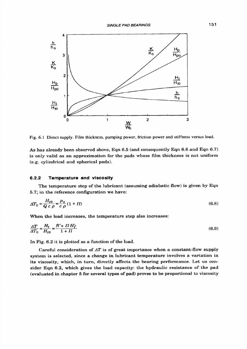
8/9/2019 Hydrostatic Lubrication 1992
http://slidepdf.com/reader/full/hydrostatic-lubrication-1992 168/558
SINGLE PAD BEARINGS
151
0
1 2
-
w,
3
Fig.
6.1
Direct supply. Film thickness, pumping power, friction power
and
stiffness versus
load.
As has already been observed above, Eqn
6.5
(and consequently Eqn
6.6
and Eqn
6.7)
is only valid
as
an approximation for the pads whose film thickness is not uniform
(e.g. cylindrical and spherical pads).
6.2.2 Temperature and viscosity
5.7; in the reference configuration we have:
The temperature step of the lubricant (assuming adiabatic flow)
is
given by Eqn
When the load increases, the temperature step also increases:
AT
Ht
R ' + n H j -
ATo
Hto
l + n
=-=
(6.9)
In Fig.
6.2
it is plotted as a fhction of the load.
Careful consideration of
AT
is of great importance when
a
constant-flow supply
system is selected, since a change in lubricant temperature involves a variation in
its
viscosity, which, in turn, directly affects the bearing performance. Let us con-
sider Eqn
6.2,
which gives the load capacity: the hydraulic resistance of the pad
(evaluated in chapter 5 for several types of pad) proves to be proportional to viscosity
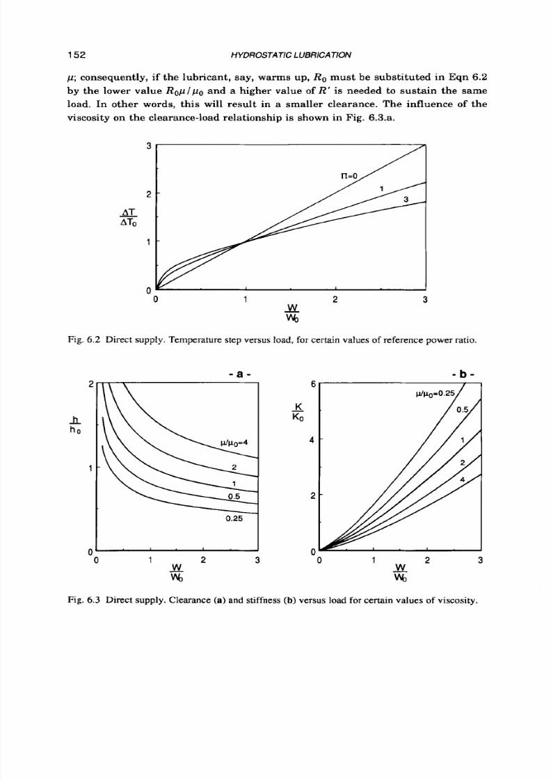
8/9/2019 Hydrostatic Lubrication 1992
http://slidepdf.com/reader/full/hydrostatic-lubrication-1992 169/558
152
HYDROSTATIC L
UBRlCATlON
,LL;
consequently, if the lubricant, say, warms up, Ro mus t be substituted in Eqn 6.2
by the lower value ROpIpO and a higher value of R ’ is needed to sustain the same
load. In other words, this will result in a smaller clearance. The influence
of
the
viscosity
on
the clearance-load relationship
is
shown in Fig.
6.3.a.
3
2
-T
AT0
1
n
0
1 2
3
Fig.
6.2 Direct supply. Temperature step versus load, for certain values of reference power ratio.
2
- t l
h0
1
0
- a -
6
-
KO
4
2
- b -
Fig.
6.3
Direct supply. Clearance
(a)
and stiffness
(b)
versus
load
for certain values of viscosity.

8/9/2019 Hydrostatic Lubrication 1992
http://slidepdf.com/reader/full/hydrostatic-lubrication-1992 170/558
SINGLE PAD BEARINGS 153
On the other hand, it is easy t o verify that
p
has no effect on pumping power
(indeed, Q s fixed and the recess pressure depends on the load alone, since
A,
is not
affected by
p);
friction power, for any given load, decreases if the temperature goes
up:
( H f is proportional to p, for a certain clearance).
Because of the reduced film thickness, stiffness is increased if viscosity is re-
duced; on the contrary, a cooler lubricant (e.g. during the starting phase) may
cause
a
considerable reduction in stiffness:
The effect of p on bearing stiffness is shown in Fig. 6.3.b.
6.3 COMPENSATED
SUPPLY
Let us now consider a pad bearing, supplied through one of the compensation
devices seen in section 2.3, rom a lubricant source, which is maintained a t a con-
stant pressure
p s .
Whatever the kind of compensation system we have, Eqn 5.1 and
Eqn 5.2 remain valid for any given pad. The recess pressure is then a fraction,
proportional t o the load, of the supply pressure:
The relationship between the hydraulic resistance of the pad (which in its turn
is closely connected to clearance
h )
and the load is easily evaluated by equating the
flow rate crossing the restrictor
Ps
P r
R r
Q
=-
to the flow rate crossing the clearances
of
the pad
We obtain:
(6.10)

8/9/2019 Hydrostatic Lubrication 1992
http://slidepdf.com/reader/full/hydrostatic-lubrication-1992 171/558
154
HYDROSTATIC LUBRICATION
The reference pressure ratio is commonly named
8 :
(6.11)
it
also represents the ratio of the design load to the limiting value
A g , .
From Eqn 6.10 and Eqn 6.11we obtain:
(6.12)
, B WIWO
R'=R pW/Wo
The hydraulic resistance of the compensation device is, in general, dependent
on flow rate and on recess pressure. Once such a relationship
is
known, as well as
the relationship between
R '
and
h ,
Eqn
6.8
allows us
t o
obtain the clearance a s a
function of the load. For the plane pads, Eqn 5.12 and Eqn 6.12 give:
The required
flow
rate,
at any given value of the load, is
Q= ----P W
1
W
h 3
(G)
o
WoR' -
Q0
Consequently, the relevant pumping power is:
(6.13)
(6.14)
(6.15)
The friction power
is
given by Eqn 5.11:
(values of Iffo or several types of pad are calculated in chapter 5 ) . Hence, the refer-
ence power ratio is
(6.16)
The temperature step, in the design configuration, is still given by Eqn 6.8,
while, for different values of the load,
(6.17)

8/9/2019 Hydrostatic Lubrication 1992
http://slidepdf.com/reader/full/hydrostatic-lubrication-1992 172/558
SlNGLE
PAD BEARINGS
155
The bearing stiffness is, on the basis
of
Eqn 5.8,
W
1
1 w a,
= 3 r
l - p w / w o + K
dW
(6.18)
It is worth noting that in order
to
obtain explicit equations connecting the bear-
ing parameters (h,
K,
etc.) to the load, knowledge
is
needed of the actual value
of
R,..
In other words, the foregoing equations need to be specialized for the various com-
pensating devices.
6.3.1
Laminar f low restrlctors (capil laries)
The recess is supplied by a source of lubricant, kept at a constant pressure
ps,
by
means of a capillary tube o r some other laminar-flow fixed restrictor. The hydraulic
resistance R, of such devices proves
t o
be a constant for any given lubricant viscosity
(see section 4.7.6). It may be expressed in terms of Ro and 8:
1.0
-
- .
h o
0.5
t
(6.19)
-
b -
3
2
K
KO
1
0
0
1
2 3 4
5
0 1 2 3 4 5
w W
OAe
PS
PS
Fig. 6.4 Capillary compensation. Bearing clearance (a) and stiffness (b) versus load.
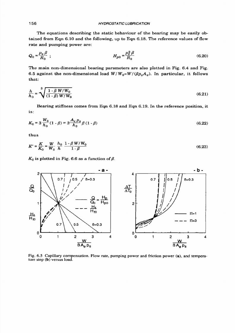
8/9/2019 Hydrostatic Lubrication 1992
http://slidepdf.com/reader/full/hydrostatic-lubrication-1992 173/558
156
HYDROSTATIC LUBRICATION
The equations describing the stat ic behaviour
of
the bearing may be easily ob-
tained from Eqn 6.10 and the following, up
t o
Eqn 6.18. The reference values
of
flow
rate and pumping power are:
(6.20)
The main non-dimensional bearing parameters are also plotted in Fig. 6.4 and Fig.
6.5 against the non-dimensional load W/ Wo=W/(jlpsAe).In particular, it follows
that:
n
(6.21)
Bearing stiffness comes from Eqn 6.18 and Eqn 6.19. In the reference position, it
is:
thus
(6.22)
(6.23)
KO is plotted in Fig. 6.6 as a hnction
of
8.
- b -
0
1 2 3
4
0
1 2 3
4
W W
BA,
Ps
0 4 s
Fig. 6.5 Capillary compensation . Flow rate, pumping power and friction power (a), and tempera-
ture step
(b)
versus load.

8/9/2019 Hydrostatic Lubrication 1992
http://slidepdf.com/reader/full/hydrostatic-lubrication-1992 174/558
SINGLE PAD BEARINGS 157
0.0 0.5
1
o
f3
Fig. 6.6
Reference values of stiffness
versus design
pressure ratio for capillary
and
orifice
compensation.
When the temperature of the lubricant is different from its design value, both
the hydraulic resistances of the restrictor and of the bearing gaps vary as does lu-
bricant viscosity
p.
The effect of such a viscosity change is easily evaluated by substi-
tuting
Rop po
and € € f o p /
o
for
Ro
and H f o , respectively, in the foregoing equations.
It
is
easy
t o
see that the clearance, as well as the stiffness, do not depend on the
actual value of
p .
Flow rate and pumping power are proportional
t o
l / p . Friction
power
is
proportional
to
p and the power ratio is therefore proportional to p2.
6.3.2 Orif ices
When orifices are used instead of laminar restrictors, it should be borne in
mind that the hydraulic resistance R , of such devices is no longer independent from
the recess pressure. The flow rate through these devices is proportional
t o
the
square root of the pressure drop ps -pr (see section 4.11).Since in the reference con-
figuration we must have
the hydraulic resistance
of
a sharp-edge orifice may be written in the following
form:
(6.24)

8/9/2019 Hydrostatic Lubrication 1992
http://slidepdf.com/reader/full/hydrostatic-lubrication-1992 175/558
158
HYDROSTATIC LUBRICATlON
By introducing Eqn
6.24
into Eqn
6.13,
the relationship between clearance and load
may be explicitly rewritten as:
(6.25)
The other bearing parameters can now be obtained straightforwardly (Eqn
6.14
t o Eqn
6.18)
and are also plotted in Fig.
6.6,
Fig
6.7
and Fig.
6.8.
In particular, stiff-
ness becomes:
where
(6.26)
(6.27)
is its reference value. The orifices are clearly characterized by greater stiffness than
the laminar-flow restrictors (see Fig.
6.6).
On the other hand, a more careful control
of the lubricant temperature
is now
required.
L
1.0
-
- .
ho .
0.5
-
- a -
3
2
K
KO
1
a
- b -
0
1
2 3 4 5 0 1
2 3 4 5
W
OA,
P s
W
OA,
Ps
Fig.
6.7
Orifice com pensation. Bearing clearance (a) and stiffness (b) versus load.

8/9/2019 Hydrostatic Lubrication 1992
http://slidepdf.com/reader/full/hydrostatic-lubrication-1992 176/558
SINGLE PAD BEARINGS
159
4
9
QO
1
L
HfO
c
- a -
I 1
0.7 / 0.5 /'"=0.3
1
2
3
4
0
1
2
3
4
W W
flAe PS flAe
PS
Fig. 6.8 Orifice compensation. Flow rate, pumping power and friction power (a), and temperature
step (b) versus load.
0
1 2 3 4
JL
PO
Fig.
6.9
Orifice compensation. Effect of viscosity (temperature) on clearance and stiffness.
Unlike laminar restrictors, the temperature of the lubricant affects the load
capacity of the bearing. The hydraulic resistance of the pad
is
proportional to the
viscosity of the lubricant, which in turn depends on temperature; this last, on the
contrary, has no practical effect on
R,.
Consequently, if
a
viscosity
p
occurs, differ-
ent from the design value po, each value
W
of the load will be sustained with a
clearance which does not tally with the value calculated by means of th e preceding
8/9/2019 Hydrostatic Lubrication 1992
http://slidepdf.com/reader/full/hydrostatic-lubrication-1992 177/558
160
HYDROSTATIC LUBRICATlON
equations. It is easy to see that the actual film thickness is proportional to the cubic
root of the viscosity; the opposite applies for stiffness (see Fig. 6.91,whereas the flow
rate does not vary. Actually, we have
P s P r
Rr
Q
=-
but R, depends on pressure drop p s - p r alone; this last depends on the applied load
and is not related to viscosity. In brief, the consequences of a change in lubricant
temperature are the following: a cooler lubricant causes lower stiffness; a warmer
lubricant causes smaller clearance and, consequently, higher friction and higher
temperature step.
6.3.3 Constant f l ow valves
A simple constant flow device is shown in Fig.
2.11.
The spool compares force
F ,
exerted by the spring with the action of the differential pressure p v - p r on spool area
A,. If restrictor
R V 1
aries much more rapidly with spool displacement than spring
force
F,,
differential pressure p v - p r = F , A , is practically kept constant; the same
occurs for flow rate Q, which depends on pressure drop p v - p r across reference re-
strictor R,.
If
R,
s a true sharp-edged orifice, and its bore diameter
is
small enough
t o
ensure that the discharge coefficient
Cd
is not dependent on the Reynolds number
(see F'ig 4.161,
Q
does not actually depend on any change in lubricant viscosity. In-
deed, we have (Eqn 4.76):
Q can be adjusted by setting up the spring force. However, since the orifice sec-
tion
A,
cannot be too small
( to
avoid an excessive drop in pressure in the device),
and true sharp-edged orifices are difficult
t o
build (and to maintain), a certain
dependence on p often exists (see Fig. 4.16 and Fig. 4.17), at least near the lower end
of the flow ra te range. If, on the other hand, R, is a laminar-flow restrictor, its
hydraulic resistance becomes a constant, and thus, for a capillary restrictor, Eqn
4.66 gives:
i.e. Q becomes inversely proportional t o viscosity (in the last equation, 1 and d are the
length and equivalent diameter of the restrictor). It should be noted that, when a

8/9/2019 Hydrostatic Lubrication 1992
http://slidepdf.com/reader/full/hydrostatic-lubrication-1992 178/558
SINGLE
PAD EEARINGS
I61
hydrostatic pad has
to
be supplied, the proportionality
of Q
and
p
ensures that the
bearing stiffness
is
independent from lubricant temperature.
As
long
as
recess pressure
p r
is
lower than
p s - F v / A , ,
the bearing simply be-
haves like a constant flow system:
Ps
B
Q = & o = R ,
P2
H~ =
H~~
=&-
(6.28)
(6.29)
(6.30)
(6.31)
(5.11rep.)
(6.32)
(6.6 rep.)
(6.7
rep.)
Once Fv is fixed, pressure drop Ap=pV-pr=Fv
A v
is a characteristic parameter
of
the device (in most cases, a few bars). Of course, it mu s t always be pv<ps; thus,
when the load increases to approach the value
(6.33)
the device ceases
t o
produce a constant flow rate, with a sharp drop in stiffness.
In Fig.
6.10
clearance and stiffness are plotted versus load. Dashed lines repre-
sent indicatively the limit behaviour
of
the valve
for
a number
of
values of @, for the
sample case Ap=O.lps.

8/9/2019 Hydrostatic Lubrication 1992
http://slidepdf.com/reader/full/hydrostatic-lubrication-1992 179/558
8/9/2019 Hydrostatic Lubrication 1992
http://slidepdf.com/reader/full/hydrostatic-lubrication-1992 180/558
SINGLE
PAD
BEARINGS
163
R,.=C,x (6.34)
On the other hand, for the equilibrium of the spool, the force exerted on it by the
spring
is:
where FvS is the spring force for complete spool displacement ( x = O ) and K, s the
stiffness
of
the spring. Under the design load, we have
Pr=/3ps
and
Rro=Ro(1-a)/a;
thus F 0 s ,
J,
and
Ro
are connected together by the relationship:
(6.35)
If the device is such as
t o
allow us to adjust the spring force, it is possible to achieve
any design value of
Ro
(i.e. of film thickness ho)under the design load
p s A $ .
Note
that, since
R,.
is
a
laminar-flow restrictor, both Ro and C, are proportional to viscos-
ity; F,s does not then depend on lubricant temperature. The displacement of the
spool under the design load is
Combining the foregoing equations, the hydraulic resistance of the controlled
restrictor may be written as follows:
(6.36)
where
For any given value of p, low rate Q, is a characteristic parameter of the device.
Introducing Eqn 6.36 into Eqn 6.13,
it
is possible t o obtain clearance as a function of
the load:
1 a
w/wo
1
--;I
P W I W ,
(
W ) & + U
l - w o P o a
(6.37)
where
(6.38)

8/9/2019 Hydrostatic Lubrication 1992
http://slidepdf.com/reader/full/hydrostatic-lubrication-1992 181/558
164
HYDROSTATIC L UBRlCATiON
- a -
- b -
1.0
-
- .
ho .
0.5
-
1.5
0 1
2
W
fi
Ae PS
- c -
2
0
1 2
W
fi
Ae
PS
4
0.0
0
2
W
fiAe PS
- d -
10
K
-
Koc
c
c
.c
Op0.25 0.3 0.4
. .
, , 0 . 2 ; g j (
1
2
W
fi Ae PS
Fig. 6.11
Cylindrical
spool
valve. Bearing clearance (a,
b),
flow rate
(c)
and stiffness
(d)
versus
load for certain values of valve parameter.
8/9/2019 Hydrostatic Lubrication 1992
http://slidepdf.com/reader/full/hydrostatic-lubrication-1992 182/558
SINGLE
PAD BEARINGS
165
A plot of hlho as a function of W/
o
is given in Fig. 6.11.a,b for certain values of 8
and 8,. It should be pointed out that, when we have P u = / 3 , the system produces a
flow rate which does not depend on load. The spool displacement will generally be
limited
t o
a certain range
X,+XM:
outside the relevant load range
W,+W,,
Eqn 6.37
is no longer valid and the bearing would merely perform like a capillary compen-
sated one; furthermore, for very small values of x,, the flow is no longer laminar.
The other bearing parameters (flow rate, power, etc.) are still given by Eqn 6.14
and the following equations; the flow rate is also plotted in Fig. 6.1l.c.
The bearing stiffness is obtained by combining Eqn 6.18 and Eqn 6.36. In partic-
ular, for the reference load,
it
is
(6.39)
where K O ,
s
the stiffness of the same pad supplied at the same pressure ratio 8
through a fixed restrictor (Eqn 6.22).
For
a generic load we have:
1 Pl8v
El
1-8 WOPV
W
1 WIWO p
WO 1-8
P v
1-8-
1 +
(6.40)
Nondimensional stiffness K/Ko c s plotted in Fig. 6.11.d as a function of WlWO it has
been chosen to show K / K o c instead of K in order to display the gain in stiffness of
the system, compared t o a capillary-compensated one). By tuning the elastic con-
stant of the spring, a very great, and even negative, stiffness could clearly be ob-
tained. On the other hand, the stiffness would be much smaller than KO for loading
conditions different from the reference one, and the flow rate would increase
sharply for loads greater than Wo. Furthermore, the behaviour of the bearing under
dynamic loading must be carefully considered.
Concerning the effects of a change in lubricant temperature, i t has already been
pointed out that, provided R ,
is
a laminar-flow restrictor, the ratio C, Ro does not
depend on
p ;
thus, only flow rate and power are affected, Q and
H p
being propor-
tional to Up and
H f
being proportional to
p .
Other types
of
devices have been proposed, with better performances than the
cylindrical spool. For example, let us consider the tapered spool valve (ref.
2.5)
in
Fig.
2.9.
Its hydraulic resistance may no longer be expressed by
a
linear relation-
ship such as Eqn 6.34. Provided aperture angle
a:
is
very small, we have:
(6.41)

8/9/2019 Hydrostatic Lubrication 1992
http://slidepdf.com/reader/full/hydrostatic-lubrication-1992 183/558
166
HYDROSTATIC LUBRlCATlON
- a -
0.0' ' ' . ' .
'
' .
0
1 2
W
BAe
Ps
- c -
2
9
00
1
- b -
0
2 4
W
DA.9
Ps
- d -
1 2
10
K
Koc
5
0
-5
0 1 2
W
B A e
PS
Fig.
6.12
Tapered spool valve. Bearing clearance (a,
b), flow
rate
(c)
and stiffness (d) versus load
for certain values of valve parameterg, and R,=Ro.

8/9/2019 Hydrostatic Lubrication 1992
http://slidepdf.com/reader/full/hydrostatic-lubrication-1992 184/558
SINGLE
PAD
BEARINGS
167
where
& x a l
c is the non-dimensional spool displacement. Proceeding as in the
former case, it is easy to verify that F,s (spring force for {=O), to spool displacement
in the design configuration), p and
Ro
are connected by the following equations:
The hydraulic resistance of the device may thus be rewritten as:
where
1 c Ro
Ku
2 a A ,
RJ
P s
u
=
---(i-
The clearance for any load
W
now proves t o be
(from
Eqn
6.13):
3
h - 1 1
p WlWo
Ro 1
q-
(6.42)
(6.43)
(6.44)
(6.45)
The rate of flow is still given by Eqn 6.14.The stiffness for the reference load is
again given by Eqn 6.39,whereas, for different loads, the relevant stiffness may be
evaluated by introducing Eqn 6.43 nto Eqn 6.18.Film thickness, the flow rate and
stiffness are plotted in Fig. 6.12 s functions of the load.
Again no effect follows a change in viscosity, except for different values of flow
rate and pumping power.
6.3.5 Diephragm-contro l led rest ric tors
The device shown in Fig. 2.10 ref. 2.6)works like the spool valves examined in
the previous section, but i ts hydraulic resistance varies according to a cubic law:
(6.46)
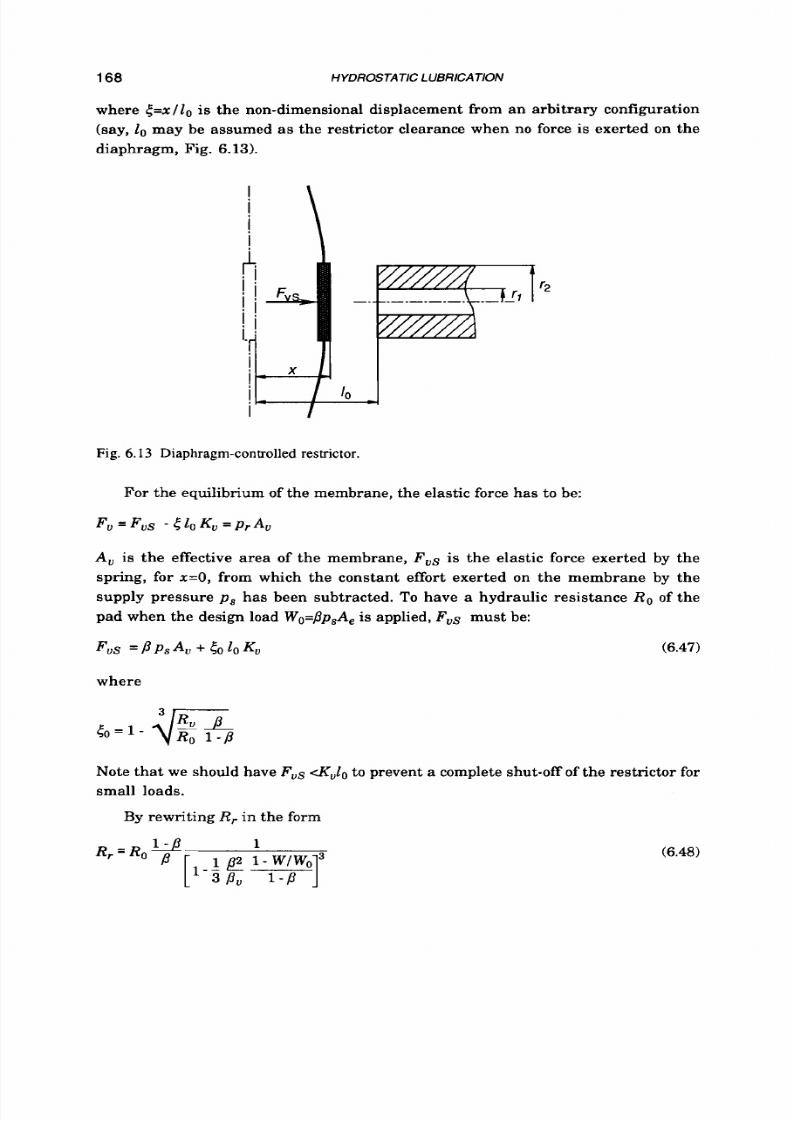
8/9/2019 Hydrostatic Lubrication 1992
http://slidepdf.com/reader/full/hydrostatic-lubrication-1992 185/558
168 HYDROSTATIC LUBRICATION
where <=x /
l o
is the non-dimensional displacement from an arbitrary configuration
(say,
lo
may be assumed as the restrictor clearance when no force
is
exerted on the
diaphragm, Fig. 6.13).
Fig. 6.13 Diaphragm-controlled restrictor.
For the equilibrium of the membrane, the elastic force has to be:
A , is the effective area of the membrane, F v s is the elastic force exerted by the
spring, for x=O , from which the constant effort exerted on the membrane by the
supply pressure
p s
has been subtracted. To have a hydraulic resistance
Ro
of the
pad when the design load Wo=ppsA, s applied, F,s must be:
F v s = P P s A ,
-k
5OlOKu
(6.47)
where
Note that we should have Fus cKv lo o prevent a complete shut-offof the restrictor for
small loads.
By rewriting R , in the form
1-8
1
1
- P
(6.48)

8/9/2019 Hydrostatic Lubrication 1992
http://slidepdf.com/reader/full/hydrostatic-lubrication-1992 186/558
SINGLE
PAD
BEARINGS 169
where
(6.49)
and by inserting it into Eqn
6.13,
ne can obtain the relationship between load and
clearance:
(6.50)
A plot of the film thickness , as well as of the flow rate (obtained as usual from
Eqn
6.14))
s a function of the load, is given in Fig.
6.14.
The stiffness in the reference configuration is again given by Eqn 6.391,where
Eqn 6.49 has now t o be used for
Po.
For different loads, the non-dimensional stiff-
ness is:
K W
0 1 -PIP,
h
W P
1 p
wo P u
w
11-w/wop
wo
3
1 - p
P
-8-
1--
(6.51)
Comparing Fig.
6.14
o
Fig.
6.11
and Fig.
6.12,
we see that the performance of the
diaphragm-controlled restrictor is better than that of the spool-controlled devices; in
particular, the load range is larger. Furthermore, due to the small mass of the
membrane, the dynamic behaviour should also be better.
As
happens in the case of the spool valves, any change in the temperature of the
lubricant does not affect the set-up of the device, but only flow rate and pumping
power.
6.3.6
Infinite-stiffness
devices
Certain controlled restrictors, such as the one shown in Fig.
2.12
(ref.
2.81,
are
able
to
keep bearing film thickness constant for a wide range
of
loading conditions.
For
the equilibrium of the spool we must have:
(6.52)
When the load, and therefore p r , vary, the spool is displaced, changing the inlet
restrictor
of
the device, until Eqn
6.52
s again fulfilled. The flow rate is:
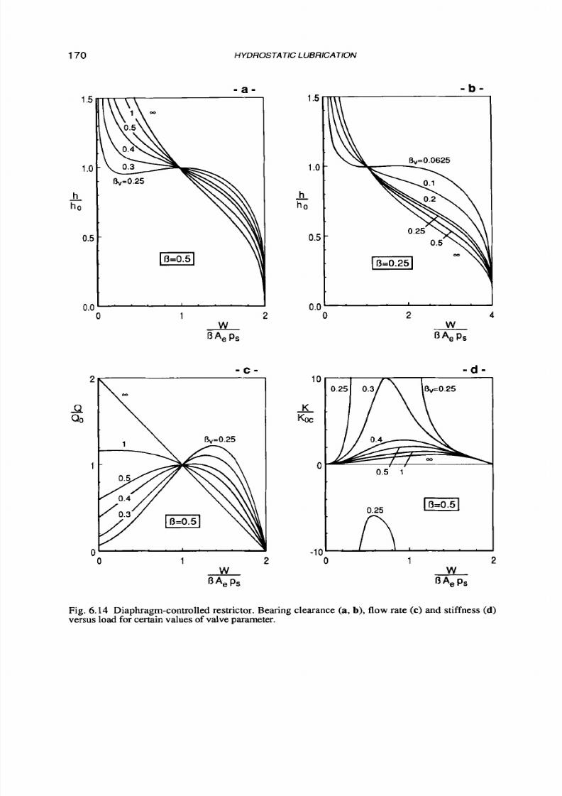
8/9/2019 Hydrostatic Lubrication 1992
http://slidepdf.com/reader/full/hydrostatic-lubrication-1992 187/558
170
HYDROSTATIC LUBRICA TlON
- a -
- b -
0
1 2
W
DAe P S
- c -
2
9
Qo
1
0
\
1
2
W
flAe
PS
1.5
1 o
h
h0
-
0.5
OS
1C
K
-
Koc
(
-1
2 4
W
OAe PS
- d -
0.5
1
p z q
0.25
n.
1 2
W
flA, Ps
Fig. 6.14 Diaphragm -controlled restrictor. B earing clearance (a, b),
flow
rate
(c)
and stiffness (d)
versus load for certain values of valve parameter.

8/9/2019 Hydrostatic Lubrication 1992
http://slidepdf.com/reader/full/hydrostatic-lubrication-1992 188/558
SINGLE PAD BEARINGS
171
1 o
0.5
*
\ \ \
.
y p 0 . 2 5
\ 0 . 5 \
0.75\
\ \ \
" \
\ \
'
' \
\
\'
\\
\
1
o
0.0
0.0
0.5
- &
Ae PS
- b -
0.5
1 o
W
-
Ae
PS
Fig. 6.15
"Infinite-stifSness"
valv e. Bearing clearance (a)
and flow
rate (b) versus load, for certain
values
of
the
valve parameter.
P v - P r
Q
=-
R ,
This means that the hydraulic resistance of the pad clearances is pegged t o the
constant value
(6.53)
v
R = R o = R ,
l-~
and thus the film thickness is kept constant as well. ho can be adjusted by setting
restrictor R, . It is noteworthy that, if R , is laminar in kind, the system is not sensi-
tive
t o
any change in lubricant viscosity, except as far as
flow
rate and pumping
power are concerned.
The f low rate proves
t o
be proportional t o load W=p,.Ae:
W
Q
= A x
(6.54)
We obviously must have p u < p s , i.e. the system cannot maintain infinite stiffness
after the spool has been completely displaced. When pr>yvps, the whole hydraulic
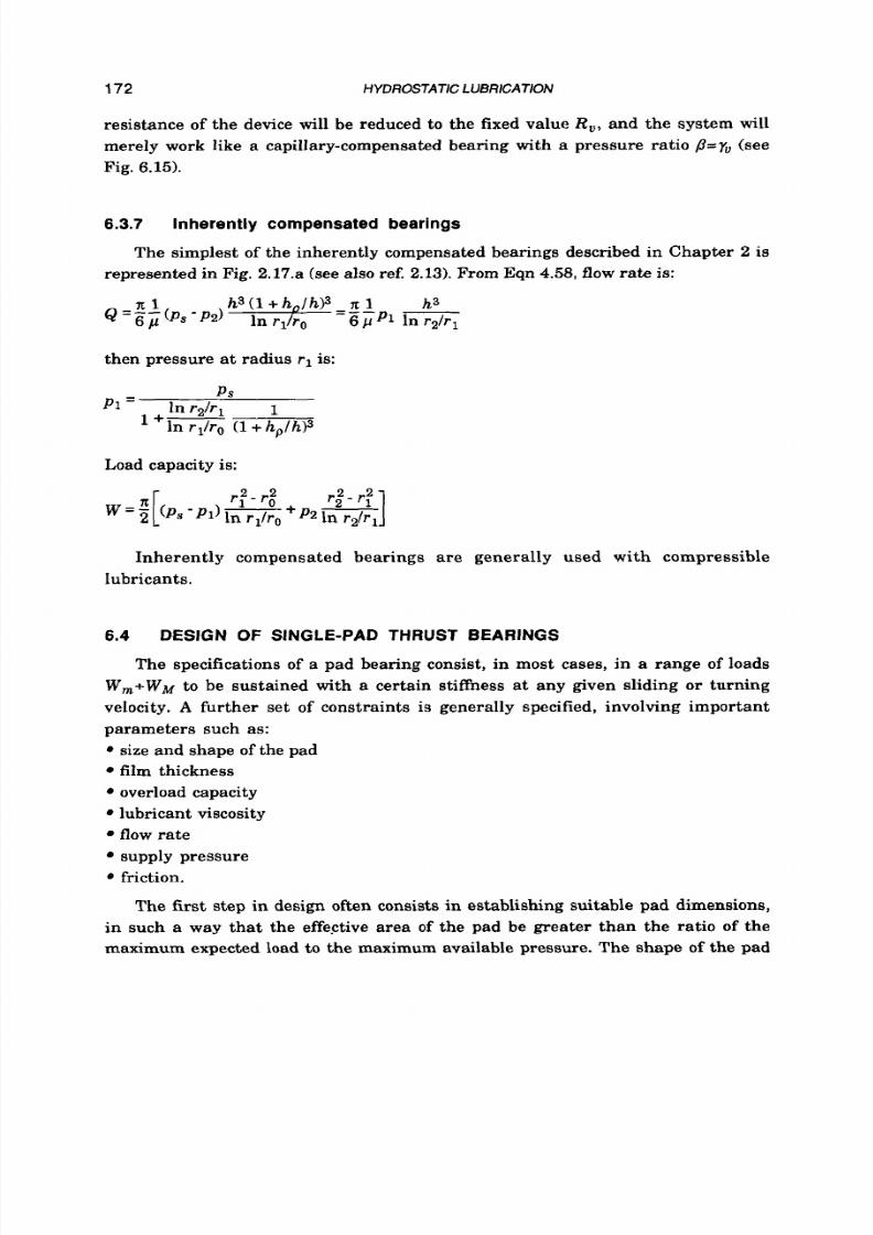
8/9/2019 Hydrostatic Lubrication 1992
http://slidepdf.com/reader/full/hydrostatic-lubrication-1992 189/558
172
HYDROSTATC
LVBRlCATlON
resistance of the device will be reduced
t o
the fixed value R,, and the system will
merely work like a capillary-compensated bearing with a pressure ratio b=y, (see
Fig.
6.15).
6.3.7 Inherent ly compensated bearings
The simplest
of
the inherently compensated bearings described in Chapter 2 is
represented in Fig. 2.17.a (see also ref. 2.13). From Eqn
4.58,
low rate is:
then pressure at radius
r l
is:
Ps
lnrz/rl 1
+E 1
+
hp/h)3
Load capacity is:
Inherently compensated bearings are generally used
w i t h
compressible
Iubricants.
6.4 DESIGN OF SINGLE-PAD THRUST BEARINGS
The specifications of a pad bearing consist, in most cases, in
a
range
of
loads
W,+WM t o be sustained with a certain stiffness at any given sliding o r turning
velocity. A further set of constraints is generally specified, involving important
parameters such as:
size and shape
of
the pad
film thickness
overload capacity
lubricant viscosity
flow rate
supply pressure
friction.
The first step in design often consists in establishing suitable pad dimensions,
in such a way that the effective area of the pad be greater than the ratio
of
the
maximum expected load
t o
the maximum available pressure. The shape of the pad

8/9/2019 Hydrostatic Lubrication 1992
http://slidepdf.com/reader/full/hydrostatic-lubrication-1992 190/558
SINGLE PAD BEARINGS 173
is often constrained. However, a few remarks on the most convenient land width to
choose may be useful.
In the foregoing sections it has been shown that, for any pad shape, the land
width ratio (e.g. parameter a' for annular-recess pads) may be chosen in such a
way as t o minimize pumping power. It is clear that when pad velocity is null, or
very low, total power consumption practically coincides with pumping power, and
then such a choice of the land width may be considered to be the optimum one.
However, this is not a critical point: for instance,
it
may be convenient to select
narrower lands to increase load capacity without affecting the external size of the
pad. On the other hand, when the speed is high enough, it is generally more conve-
nient to select narrow lands
to
minimize the total power H t = H p + H p
The selection of the thickness of the film depends on certain contrasting factors:
it must be small enough to ensure sufficient stiffness at any load to meet the
specifications;
it
must be small enough to ensure small flow rate and pumping power (of course,
this point, as well as the next, is also connected with the choice
of
lubricant
viscosity);
it must be large enough
to
avoid excessive friction;
it must be much larger than the geometric errors of the mating surfaces
(roughness, planarity, parallelism).
As
far as the problem of a suitable choice of h and
p
is concerned, it
is
possible to
demonstrate that, for any given pad and any given viscosity,
an
"optimum" clear-
ance may be calculated (from the point of view of total power) on the condition th at
H f = 3 H p .
Conversely, if
h
is given, "optimum" viscosity is the one which gives
Hf-&lp
(ref.
2.3) .
Let us now briefly examine this problem applied
to
rotating pads.
Total power in the reference configuration may be written in the form:
valid for constant-pressure supply, as well as for direct constant-flow supply (in
this
case it must be stated that
/j'=l).
or axisymmetric pads, such
as
plane or tapered
circular pads, the effective area can be written as in Eqn
5 .20 ,
and the hydraulic
resistance as in Eqn
5 .83 :
of course, the relevant equations must be used for
A*,
and
R*,
and a=d2 for plane pads. For these pads total power may hence be rewritten as:
(6.55)

8/9/2019 Hydrostatic Lubrication 1992
http://slidepdf.com/reader/full/hydrostatic-lubrication-1992 191/558
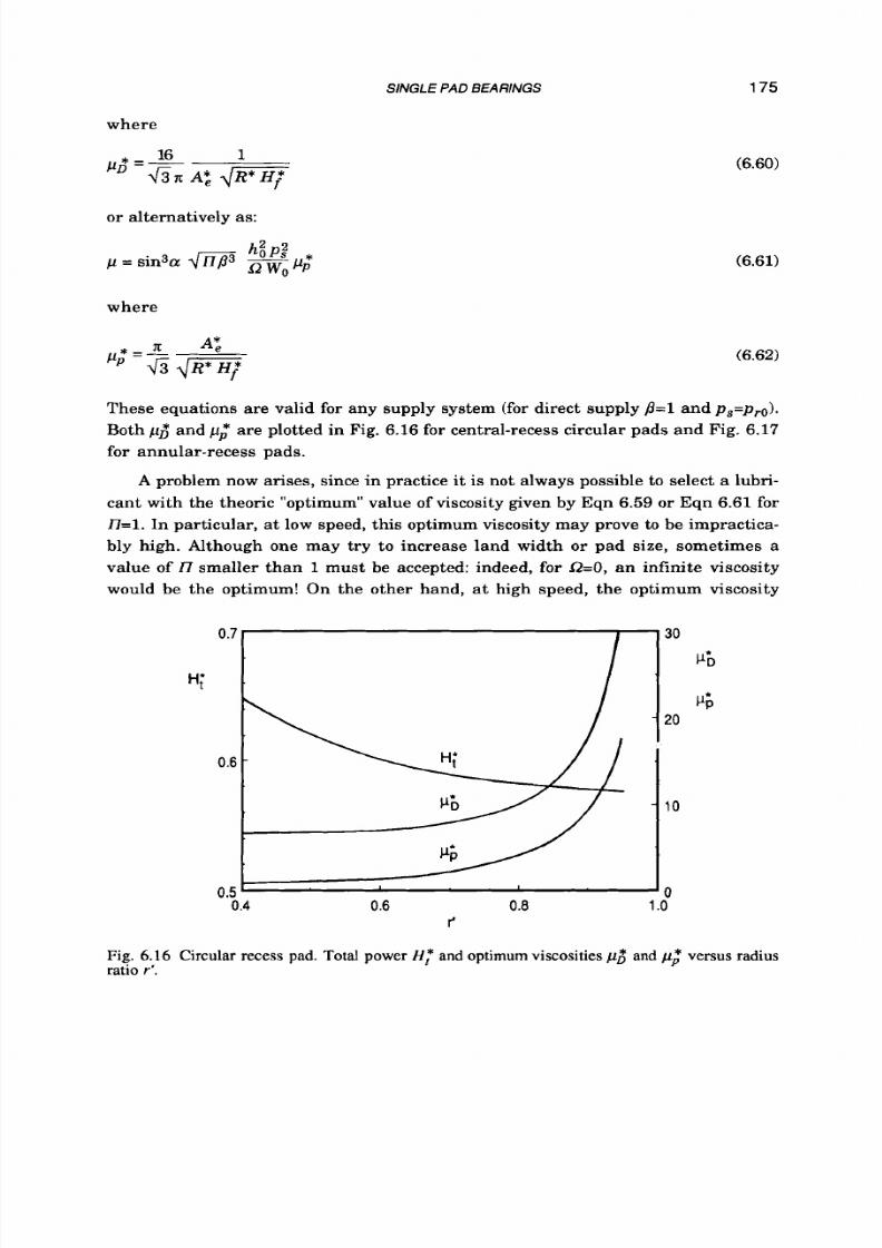
8/9/2019 Hydrostatic Lubrication 1992
http://slidepdf.com/reader/full/hydrostatic-lubrication-1992 192/558
SlNGLE PAD BEARlNGS
175
where
or alternatively as:
where
(6.60)
(6.61)
(6.62)
These equations are valid for any supply system (for direct supply
p=1
and ps=pro) .
Both
p$
and p; are plotted in Fig.
6.16
for central-recess circular pads and Fig.
6.17
€or annular-recess pads.
A problem now arises, since in practice i t is not always possible to select a lubri-
cant with the theoric "optimum" value of viscosity given by Eqn 6.59 or Eqn 6.61 for
n=1. n particular, a t low speed, this optimum viscosity may prove t o be impractica-
bly high. Although one may t r y t o increase land width or pad size, sometimes a
value of l7 smaller than 1 must be accepted: indeed, for Q=O, an infinite viscosity
would be the optimum On the other hand, a t high speed, the optimum viscosity
H i
Fig. 6.16 Circular recess pad. Total power H : and optimum viscosities p$ and p; versus
radius
ratio
r'.
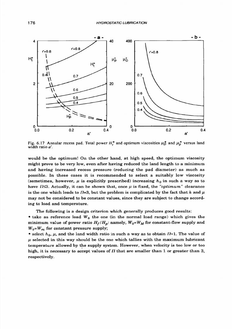
8/9/2019 Hydrostatic Lubrication 1992
http://slidepdf.com/reader/full/hydrostatic-lubrication-1992 193/558
176
HYDROSTATIC LUBRICATION
- a - - b -
4
H i
2
40
20
400
GI
200
0
0.0
0.2 0.4
"
a'
r'=O.8
\
O
0.0
0.2
0.4
a'
Fig.
6.17
Annular recess pad. Total power H: and optimum viscosities
p$
and p; versus land
width
ratio
a'.
would be the optimum On the other hand, a t high speed, the optimum viscosity
might prove to be very low, even after having reduced the land length to a minimum
and having increased recess pressure (reducing the pad diameter)
as
much
as
possible. In these cases it is recommended t o select a suitably low viscosity
(sometimes, however, p is explicitly prescribed) increasing ho in such a way as to
have n13.Actually, it can be shown that, once p is fixed, the optimum clearance
is the one which leads to n=3, ut the problem is complicated by the fact tha t
h
and p
may not be considered
to
be constant values, since they are subject t o change accord-
ing to load and temperature.
The following is a design criterion which generally produces good results:
take as reference load Wo the one (in the normal load range) which gives the
minimum value of power ratio H f / H p :namely, Wo=WM or constant-flow supply and
W,=W, for constant pressure supply;
select h,, p, and the land width ratio in such a way as
to
obtain n=1. he value of
p selected in this way should be the one which tallies with the maximum lubricant
temperature allowed by the supply system. However, when velocity
is
too low
o r
too
high,
it
is necessary to accept values of ll that are smaller than
1
or greater than
3,
respectively.

8/9/2019 Hydrostatic Lubrication 1992
http://slidepdf.com/reader/full/hydrostatic-lubrication-1992 194/558
8/9/2019 Hydrostatic Lubrication 1992
http://slidepdf.com/reader/full/hydrostatic-lubrication-1992 195/558
178 HYDUOSTA TIC LUBUlCATlON
the land width ratio) or h o and start again from point
(ii)
o r (iii). If p o p t
cannot be brought into the admissible range, because the velocity is too
small, select the highest available viscosity. On the other hand, a very high
speed would require
too
low viscosities to be optimized with
n=1,
nd conse-
quently a greater value of the power ratio must be selected; values of
n
greater than
3
should, however, be avoided, or else excessive temperature
steps could follow (Eqn
6.8);
if the supply system is not able
t o
hold the temperature of the lubricant
within narrow limits, the designer should take a certain viscosity range into
account, instead of a single value. A
simple method consists in considering
popt
as the lower limit of the viscosity range, which tallies with the highest
lubricant temperature.
For
a cooler lubricant viscosity will be greater, as
well as film thickness and, above all, bearing stiffness will be lower. Conse-
quently, it is necessary to check K for the whole temperature range;
v )
calculate the required
flow
rate;
calculate pumping power
H p o
and friction power
H f o
(for circular bearings
Eqn
6.57
and Fig.
6.16 o r
Fig 6.17 give total power
Hto:
now
Hpo=HtoI(l+17)
and
Hfo=Hto17).
For loads smaller than
Wo,
both the powers will be lower;
check the maximum temperature step in the lubricant (Eqn 6.9);
if
a
range of viscosities is to be allowed in the plant, check friction power and
temperature step for the maximum viscosity too;
vi)
check the Reynolds number;
for bearings rotating at high speed also check the effect of inertia forces
(parameter
S i )
and the circumferential Reynolds number;
vii) check the dynamic behaviour of the system (see chapter
10).
In certain cases it may be necessary to have a
flow
rate which differs from the
value calculated at point (v) above (for instance, because the pump which has to be
used does not feature a n adjustable
flow
rate); clearly, if this happens
it
is
necessary
to repeat the calculations (in particular, as far
as
film thickness and stiffness are
concerned) using the actual value
of
the flow rate. If the difference is large, it may
be considered convenient to modify viscosity
o r
geometrical parameters in order to
approach the
opt imum
value of the power ratio again.
EXAMPLE
6.1
Design a circular-recess pad to sustain a thrust varying in the
W,=30
K N
t
W ~ = 4 0
v range at a speed G=lO a d f s , w i t h a friction m oment
lower
than 1 N m .
Further constraints are the following: the outer diameter must be DSlOO mm; the
lubricant viscosity can be chosen in a range of 0 . 0 2 4 1 N s lm 2 ; th e d isp la cem en t a s
8/9/2019 Hydrostatic Lubrication 1992
http://slidepdf.com/reader/full/hydrostatic-lubrication-1992 196/558
SINGLE PAD BEARINGS 179
the load varies (slowly) from the minimum to the maximum value must be smaller
than
10 pm; the recess pressure must always be smaller than 7 MPa.
i) Since the turning velocity is low, a first trial value for r' could be r'=0.5, and
hence A2=0.541. In order to sustain the maximum load WO=wM=40
KN,
the effective
area must be greater than w 0 / 7 MPa, i.e. A ,~5 .7.10-~2; consequently, due to the
limited diameter, it must be (Eqn 5.20) A*,>0.727, and a considerably larger value is
needed for r' (Fig. 5.1. b).
ii) Let
us
select D=lOO mm, r'=O.75; it is easily obtained (from Fig. 5.1.6 or by
means of the relevant equations) A50.760, R*=0.288, Hf*=0.684; he effective area is
then A,=5.97.10-3 m2 and the maximum recess pressure is pro=WolA,=6.70 MPa.
iii) A suitable value for minimum film thickness may be ho=30pm. The maxi-
mum film thickness, which tallies with the minimum load Wm=30
KN,
is (Fig.
6.1)
h~=1 .10.ho=33 m. Note that the displacement h ~ - h o = 3m is much smaller than
required.
iv) In
Fig.
6.16 we may read &=8.72, i.e. bpt=0.31Nslm2. This last value is too
high,
hence the
maximum
allowable ualue p=O.1 Ns lm2 should be selected, accept-
ing a power ratio smaller than 1 (the friction power will prove to be much smaller
than the pumping power).
v) The reference hydraulic resistance is easily calculated as Ro=2.03.1012Nslm5
(Eqn 5.21), and hence Q=prolRo=3.29.10-6m3/s , Hpo=proQ=22W. As far as friction is
concerned, we have Mf0=0.22Nm, Hf0=2.2 W. Obuiously, for loads smaller than Wo,
both Hp and H f will be smaller. The temperature step is maximum in correspon-
dence to the max imum load: from Eqn 6.8, assuming c.p=l.7.10-3 J lm2 C,
dTod.3"c.
EXAMPLE 6.2
Design an annular-recess bearing to sustain a load W=75
K N
with stiffness
K0>5.109N lm , at a speed l2=628 radl s (6000 rpm). The outer diameter of the pad
must be smaller than 200 mm, and the inner one greater than 120 mm. The maxi-
mum recess pressure can be as high as 12 MPa, but the bearing should be able to
sustain, exceptionally, a maximum overload dW~=75 N . the data of the lubricant
to be used are: p=0.02+0.03 N s lm2 (depending on the actual operating temperature),
p
=go0
e l m 9 c=1890JlQOC.
i) Since the speed is high, let us start with a small value of a', say a'=0.1. I f the
greatest allowable pad area is chosen, it follows that r'=120/200=0.6.
ii)
It follows immediately that: A*,=0.576 and A,=0.0181 m2. The maximum load
WE=150
KtV
hence tallies with a recess pressure p~=8.29MPa; for the normal load
Wo we have pr0=4.14 MPa.
iii) Since Ko=3W0Ih, o obtain the required stiffness we must have hoc45 pm.
However, since a wide viscosity range is expected, to obtain hc45p or the highest
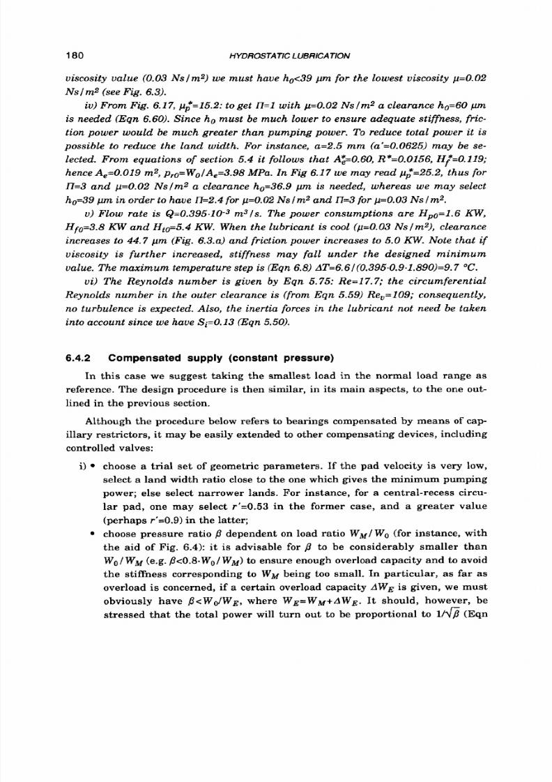
8/9/2019 Hydrostatic Lubrication 1992
http://slidepdf.com/reader/full/hydrostatic-lubrication-1992 197/558
180 HYDROSTATIC LUBRICATION
viscosity value (0.03 Nslm2) we must have ho<39
pm
for the lowest viscosity p=0.02
Ns I m2 (see Fig. 6.3).
iv) From Fig. 6.1 7, p:=15.2: to get
I l = l
with p=0.02 Ns lm 2 a clearance ho=60pm
is needed (Eqn
6.60).
Since ho must be
much
lower to ensure adequate stiffness, fric-
tion power would be much greater than pumping power. To reduce total power it is
possible to reduce the land width. For instance, a=2.5 mm (a'=0.0625) may be se-
lected. From equations of section
5.4
it follows that A:=0.60, R*=0.0156, Hf*=0.119;
hence Ae=0.019 m2, pro=WolAe=3.98MPa. In Fig 6.17 we may read pz=25.2, thus for
l7=3 and p=0.02 Nslm2 a clearance ho=36.9 pm is needed, whereas we may select
ho=39pm in order to have Il=2.4 for p=0.02
Ns
m2 and n=3or
p=0.03
Ns
I
m2.
v )
Flow rate is &=0.395.10-3 mats. The power consumptions are Hp0=l.6
KW,
Hf0=3.8KW and Ht0=5.4KW. When the lubricant is cool (p=0.03 Ns lm 2), clearance
increases to 44.7 pm (Fig. 6.3.a) and friction power increases to 5.0 KW. Note that if
viscosity is further increased, stiffness may fall under the designed min imum
value. The maximum temperature step is (Eqn 6.8)AT=6.61(0.395.0.9.1.890)=9.7
C.
ui) The Reynolds number is given by Eqn 5.75: Re=17.7; the circumferential
Reynolds number in the outer clearance is (from Eqn 5.591 Re,=109; consequently,
no turbulence is expected. Also, the inertia forces in the lubricant not need be taken
into account since we have Si=O.13 (Eqn 5.50).
6.4.2 Compensated supply (constant pressure)
In this case we suggest taking the smallest load in the normal load range as
reference. The design procedure is then similar, in its main aspects, to the one out-
lined in the previous section.
Although the procedure below refers t o bearings compensated by means
of
cap-
illary restrictors,
it
may be easily extended to other compensating devices, including
controlled valves:
i)
choose a trial set of geometric parameters. If the pad velocity
is
very low,
select a land width ratio close to the one which gives the minimum pumping
power; else select narrower lands. For instance, for a central-recess circu-
lar pad, one may select
r'=0.53
in the former case, and a greater value
(perhaps r'=0.9)in the latter;
dependent on load ratio WMIWo (for instance, with
the aid of Fig. 6.4): i t is advisable for to be considerably smaller than
Wo1WM e.g.
8 ~ 0 . 8 .
o/W M )o ensure enough overload capacity and to avoid
the stiffness corresponding to W M being too small. In particular, as far as
overload is concerned, if a certain overload capacity
AWE is
given, we must
obviously have PCWOIWE,where WE=WM+AWE.t should, however, be
stressed that the total power will turn out t o be proportional to l/fi (Eqn
choose pressure ratio

8/9/2019 Hydrostatic Lubrication 1992
http://slidepdf.com/reader/full/hydrostatic-lubrication-1992 198/558
SINGLE
PAD
BEARINGS
181
6.57), but, on the other hand, stiffness KO is proportional to (1-p).When the
load range is wide (i.e. when W o is much smaller than W , ) a very small
value is needed for p ; in this case, an opposed-pad bearing may be the most
suitable choice (see chapter 7);
ii) choose suitable values for effective area A , and supply pressure p s , in such a
way as to obtain Wo=AJ?p,;
evaluate the size of the pad, and check it is compatible with the specifica-
tions;
iii) select the minimum clearance h,, tallying with the maximum load WM;
evaluate the reference clearance ho (e.g.
for
capillary compensation from
Eqn 6.21 or Fig. 6.4.a). The thinner
ho
is, the smaller the power losses
(provided a sufficiently low viscosity is available) and the greater the stiff-
ness will be; on the other hand, greater manufacturing accuracy will be
required;
calculate KO (e.g. from Eqn 6.22) and stiffness
K=KoK'
tallying with load W,
(e.g. from Eqn 6.23 or Fig. 6.4.b). For controlled restrictors, the relevant
parameters (e.g. 8 , ) must also be selected;
check that stiffness is great enough for the whole load range: if it is not, one
may try to decrease p, starting again from point (i), or to decrease ho, f pos-
sible, starting again fkom point (iii);
iv) calculate the optimum viscosity, that is the value popt that makes
I7=1
(Eqn
6.4). For circular bearings, this may be done quickly with the aid of Fig. 6.16
or Fig. 6.17;
check that
k p t
is a plausible value (sometimes
p
may be directly imposed by
the specifications). If it
is
not, modify the geometrical parameters (namely
the land width ratio) or ho and start again from point (ii) o r (iii). If
p o p t
cannot be brought into the admissible range, because the velocity is too
small, select the highest available viscosity. On the other hand, a very high
speed would require too low viscosities t o be optimized with n=1, nd conse-
quently a greater value of the power ratio must be selected; values of Il
greater than 3 should, however, be avoided: otherwise excessive temperature
steps could follow;
if the supply system is not able t o hold the temperature of the lubricant
within narrow limits, the designer should take a certain viscosity range into
account, instead of a single value.
A
simple method consists in considering
popt as the lower limit of the viscosity range, which tallies with the highest
lubricant temperature.
For
a cooler lubricant viscosity will be greater: for
many compensating devices this will have no effect on clearance and stiff-

8/9/2019 Hydrostatic Lubrication 1992
http://slidepdf.com/reader/full/hydrostatic-lubrication-1992 199/558
182 HYDROSTATIC L UBRICA TION
ness; instead, the power ratio will be greater (proportional to
p2
for laminar-
flow devices);
v) calculate the flow rate;
calculate pumping power Hpoand friction power Hfo (for circular bearings
Eqn 6.57 and Fig. 6.16 o r Fig 6.17 give total power Hto: now Hpo=Hto / ( l+~)
and Hfo=Hto17).For loads greater than WO,he pumping power is smaller,
but Hf increases (Eqn 5.11);
check the maximum temperature step in the lubr icant (Eqn 6.8 and Eqn
6.17);
if a range of viscosities is to be allowed in the plant, check friction power and
the temperature step for the maximum viscosity,
too;
vi)
design the restrictor: its hydraulic resistance
RrO
must be given by Eqn
6.19;
if capillary pipes are used, select length and diameter by means of Eqn 4.67;
check the Reynolds number in the restrictor to ensure laminar flow (Eqn
4.68);
vii) check the Reynolds number;
for bearings rotating a t high speed, also check the effect of inert ia forces
(parameter
S i )
and the circumferential Reynolds number;
viii) check the dynamic behaviour of the system (see chapter 10).
EXAMPLE
6.3
A large slide is sustained by a set o f rectangular pads (supplied through capil-
lary restrictors) whose dimensions are
B=0.3
m and L=0.4 m. Each pad must
sus-
tain a load
W=60
N
with a stiffness K>2.5.109 N l m and a film thickness not
smaller than 40
pm. The friction force should not be greater than 6 N at a speed
U=0.05
m
I
s.
i) Since velocity is low, it is convenient to have large lands; if we select a'=0.15
and rL: =0.25, from Fig. 5.27 we obtain Az=0.645. Since no great load variations are
expected, we may try to select a relatively high value, such as 8=0.6, for the pressure
ratio.
ii ) The pad dimensions are given: the effective area is A,=LBA:=0.077 m2. The
supply pressure should hence be p,=1.29 Pa.
iii) I f we select ho=40pm, Eqn 6.22 immediately gives K0=1.8.109 N l m , which is
not enough. Hence it is necessary to select a smaller value for
p,
such as p=0.4.
Repeating the above calculations, we now get: ps=1.95 MPa and Ko=2.7.1@ N l m.
iv) From Fig. 5.28 we obtain R*=0.75, and from Eqn 5.108 (stating h,=l mm)
Af=0.079 m2. Since the friction force must be smaller than
6
N,
Eqn 5.106 gives an
upper boundary for viscosity: p=0.0607 Nslm2. For such a viscosity Eqn 6.16 gives
n=0.14 (of course, the pumping power will prove to be much greater than the fric-

8/9/2019 Hydrostatic Lubrication 1992
http://slidepdf.com/reader/full/hydrostatic-lubrication-1992 200/558
SINGLE
PAD
BEARINGS 183
tion power). A lubricant is therefore selected, whose viscosity is
p=0.06
Nsl m2 at the
lowest operating temperature.
v ) Calculations of flow rate and power are now straightforward, leading to:
Qo=1.1.10-6 m3/ s; Hp=2.1 W, H ~ 0 . 3 . Temperature step proves to be slightly
greater than 1
C
assuming c.p=1.7.106 Jlm3 C). For lower viscosities H f decreases
while Q and Hpprove to be proportional to 1I p.
vi) The hydraulic resistance
of
the restrictor
can
be calculated by means of Eqn
5.102 and Eqn 6.19, which lead to R,/p=17.6.1012 m-3. From Eqn 4.67 it follows that
such a hydraulic resistance may be obtained with a pipe 27
mm
in length and with
a 0.5
mm
bore. The Reynolds number, calculated by assuming p=0.06 Nslm2 and
p 9 0 0 Kglm3,
is
Re=42, considerably less than its critical value.
EXAMPLE 6.4
Design a capillary-compensated annular-recess bearing to sustain a load which
varies i n the 2 0 4 5 KN range, with a displacement Ah smaller than 20
pm.
The
outer pad diameter must be smaller than 0.2 m, and the inner diameter must be
equal to 0.1 mm. A further requirement is that the friction moment needed to rotate
the bearing at e 6 2 8 radls (6000 pm) must be smaller than 5 Nm. The supply sys-
tem to be used delivers lubricant at pressure ps=4 MPa; viscosity is expected to vary
in the p=0.0154.020 Ns 1m2 range, depending on actual operating conditions; den-
sity and specific heat are p=920KgIm3andc=1850 JIKgOC.
i) Since the speed is high, choose narrow lands, say a=2 mm. The load ratio
i s
WMIWo=1.75,hence p=0.45 should be a proper selection (see Fig. 6.4).
i i )
Wi th the give n supply pressure, the effecti ve area should be
Ae=2~/(O.45.4.1O6)0.0111 m2. For the sake of simplicity, let us choose D=0.16 m
(i.e. r'=O.625; a'=0.067), obtaining Az=0.569, R*=0.0154, Hf*=0.122;hence, A,=0.0114
m2 and p=0.437.
iii) From Eqn 6.21 (or Fig. 6.4.a), for any certain design clearance ho the mini-
mum clearance (which tallies with the maximum load) is hm=0.62.ho. To ensure
Ah=ho-hm<20 pm we must therefore have ho152.7 pm. On the other hand, to have
Mf<5 N m for p=0.02 Ns lm 2, the minimum film thickness cannot be smaller than
19.8 pm, i.e ho must be not smaller than 31.8 pm (see Eqn 5.70).
iv) From Fig. 6.17, pJ=119; to have ll=1 for p=0.015 Nslm2 we should have (Eqn
6.59) ho=41.4 pm. Selecting ho=40 pm, the reference power ratio will vary in the
1.1411712.04 range, depending on the actual value of the viscosity. Flow rate, powers
and temperature step depend on load and viscosity and are summarized in the fol-
lowing table.
v) The hydraulic resistance of the restrictor must be R,=1.29.Ro (Eqn 6.19), i.e.
R,.=8.87.109 Ns lm5 for p=0.015 Nslm2. Note that, due to the high value of the flow
rate, such a restrictor cannot be made with a small pipe without accepting high
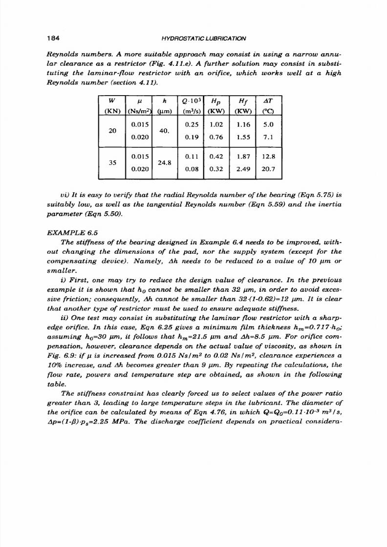
8/9/2019 Hydrostatic Lubrication 1992
http://slidepdf.com/reader/full/hydrostatic-lubrication-1992 201/558
184
HYDROSTATIC LUBRICATION
W
(KN)
20
35
Reynolds numbers. A more suitable approach may consist in using a narrow annu-
lar clearance as a restrictor (Fig. 4.11.e). A further solution may consist in substi-
tuting the laminar-flow restrictor with an orifice, which works well at a high
Reynolds number (section 4.11).
p h Q.103 H p H f AT
(Ns/m2) (m3/s) (KW) (KW) ("(2
0.015 0.25 1.02 1.16 5.0
0.020 0.19 0.76 1.55 7.1
40.
0.015
0.11 0.42
1.87 12.8
0.020 0.08 0.32 2.49 20.7
24.8
vi) It is easy to verifv that the radial Reynolds number of the bearing (Eqn 5.75) is
suitably low, as well as the tangential Reynolds number (Eqn 5.59) and the inertia
parameter (Eqn 5.50).
EXAMPLE 6.5
The stiffness
o f
the bearing designed in Example 6.4 needs to be improved, with-
out changing the dimensions
o f
the pad, nor the supply system (except for the
compensating device). Namely, Ah needs to be reduced to a value of 10 pm or
smaller.
i) First, one may try to reduce the design value of clearance. In the previous
example it is shown that ho cannot be smaller than 32 pm, in order to avo& exces-
sive friction; consequently, Ah cannot be smaller than 32.(1-0.62)=12
pm.
It
is
clear
that another type of restrictor must be used to emure adequate stiffness.
W One test may consist in substituting the laminar f low restrictor with a sharp-
edge orifice. In this case, Eqn 6.25 gives a minimum film thickness hm=O.717.h0;
assuming ho=30 pm, it follows that h,=21.5 pm and Ah=8.5 pm. For orifice com-
pensation, however, clearance depends on the actual value of viscosity, as shown in
Fig.
6.9: i f p
is increased from 0.015 NsIm2 to 0.02 Nslm2, clearance experiences a
10% increase, and Ah becomes greater than 9 pm. By repeating the calculations, the
flow
rate, powers and temperature step are obtained, as shown in the following
table.
The stiffness constraint has clearly forced us to select values of the power ratio
greater than 3, leading to large temperature steps in the lubricant. The diameter of
the orifice can be calculated by means of Eqn 4.76, in which Q=Qo=O.ll m3/s ,
Ap=(l p)p,=2.25 MPa. The discharge coefficient depends on practical considera-
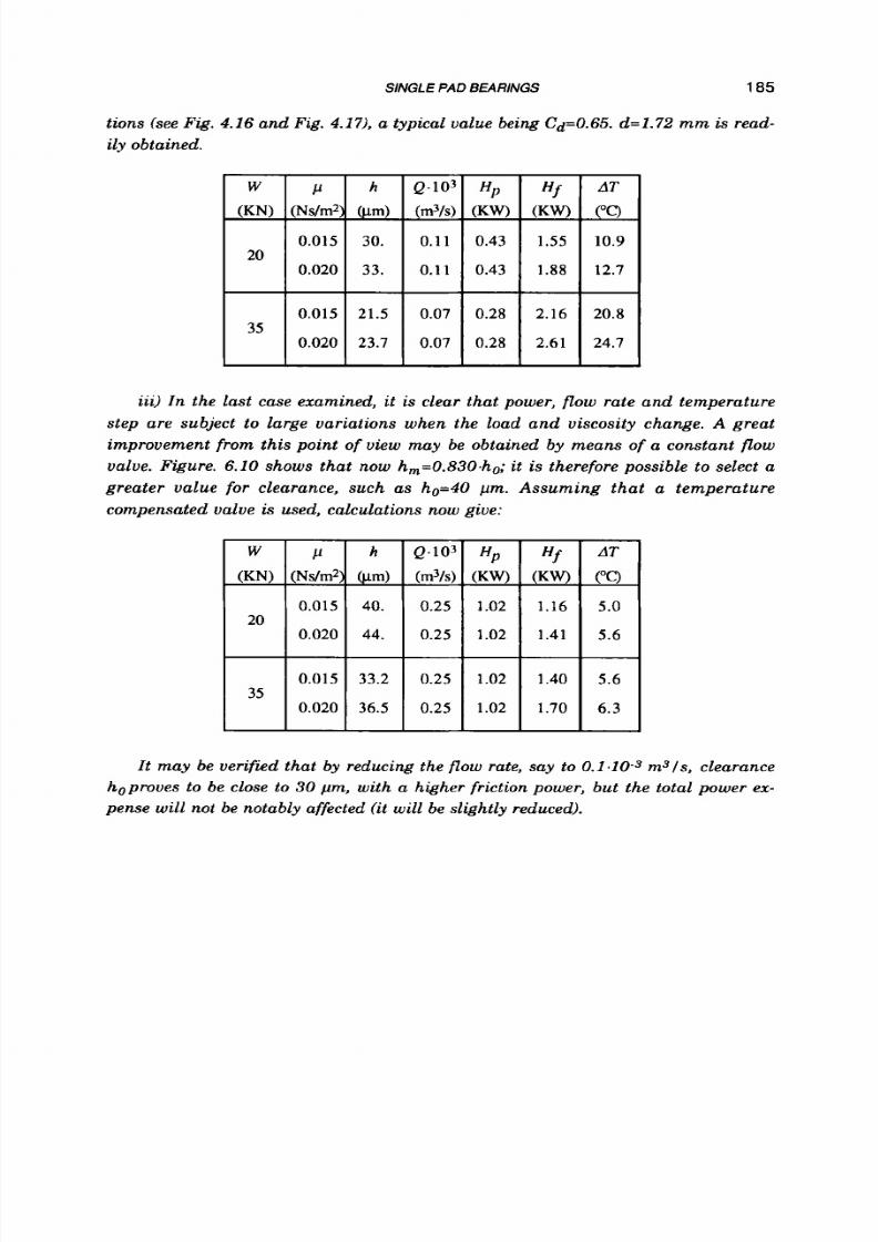
8/9/2019 Hydrostatic Lubrication 1992
http://slidepdf.com/reader/full/hydrostatic-lubrication-1992 202/558
SlNGL
E
PAD
BEARlNGS
185
W
(KN)
20
35
tions (see Fig. 4.16 and Fig. 4.17), a typical value being Cd=0.65. d=1.72 mm is read-
ily obtained.
p
h
Q.103
H p
Hf
AT
(Ns/m2) (pm)
(m3/s) (KW) (KW)
(T)
0.015 30. 0.11 0.43
1.55
10.9
0.020
33. 0.11
0.43
1.88
12.7
0.015 21.5
0.07 0.28 2.16 20.8
0.020 23.7
0.07 0.28 2.61 24.7
iii) In the last case examined, it is clear that power, flow rate and temperature
step are subject
to
large variations when the load and viscosity change. A great
improvement from this point of view may be obtained by means of a constant flow
valve. Figure. 6.10 shows that now h,=0.830.ho; it is therefore possible to select a
greater value for clearance, such as ho=40 pm. Assuming that a temperature
compensated valve is used, calculations now give:
It may be verified that by reducing the flow rate, say to 0.1 l O - 3 m3/s, clearance
hoproues to be close to 30 pm, with a higher friction power, but the total power ex-
pense will not be notably affected (it will be slightly reduced).

8/9/2019 Hydrostatic Lubrication 1992
http://slidepdf.com/reader/full/hydrostatic-lubrication-1992 203/558
Chapter
7
OPPOSED-PAD AND MULTIPAD BEARINGS
7.1
INTRODUCTION
A multipad bearing system is made up of a certain number of pads, with a
common moving member. The pads may be, in general, quite different, and they,
too,
might be fed by means of differing devices.
All
these bearings may be studied by applying
to
each pad the equations already
developed for the single pads in chapter 5 , and by summing together the effects of all
the pads, after having expressed all the pad clearances as functions of the dis-
placement of the moving member.
The case of the opposed-pad bearings is of particular importance.
7.2
OPPOSED-PAD BEARINGS
For
any opposed-pad bearing, such as the one in Fig. 7.1, the total load capacity
is, obviously,
The
flow
rate is, from Eqn
5.2
and Eqn 5.10,
(7.2)

8/9/2019 Hydrostatic Lubrication 1992
http://slidepdf.com/reader/full/hydrostatic-lubrication-1992 204/558
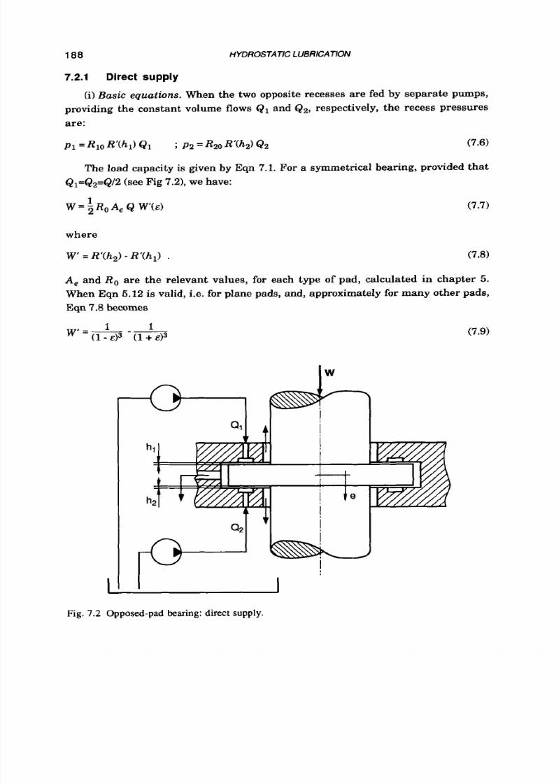
8/9/2019 Hydrostatic Lubrication 1992
http://slidepdf.com/reader/full/hydrostatic-lubrication-1992 205/558
188
HYDROSTATIC LUB RICATlON
7.2.1 Direct supply
(i)Basic equations. When the two opposite recesses are fed by separate pumps,
providing the constant volume flows Q1
and
Q2,
respectively, the recess pressures
are:
The load capacity is given by Eqn 7.1. For a symmetrical bearing, provided that
Q1=Q2=Q/2(see Fig 7.21, we have:
(7.7)
W = i j R o A , Q W ( E )
where
A,
and
Ro
are the relevant values, for each type of pad, calculated in chapter
5.
When
Eqn 5.12 is
valid,
i.e.
for plane pads, and, approximately for many other pads,
Eqn 7.8
becomes
Fig.
7.2
Opposed-pad bearing: direct supply.

8/9/2019 Hydrostatic Lubrication 1992
http://slidepdf.com/reader/full/hydrostatic-lubrication-1992 206/558
OPPOSED-PAD AND MULTIPAD BEARINGS
189
In the rest of this chapter, Eqn 5.12 will be considered to be valid.
The bearing stiffness, calculated by means of Eqn 7.5, may be put, as usual, in
the following form:
K = KO K ( E ) (7.10)
where
is the stiffness in the unloaded configuration (E=O) , and
The pumping power is now expressed by the equation:
where
For the friction power, we have:
H f
= 2
H fo H i
( E )
where
1 1
1
Hi.
' Z ( E +F )
Again,
H f o
s the relevant value of the single pads (see chapter 5).
The power ratio in the reference configuration is, quite obviously,
Hfo
Ro Q2
n=4
and the relevant temperature
step is
(7.11)
(7.12)
(7.13)
(7.14)
(7.15)
(7.16)
(7.17)
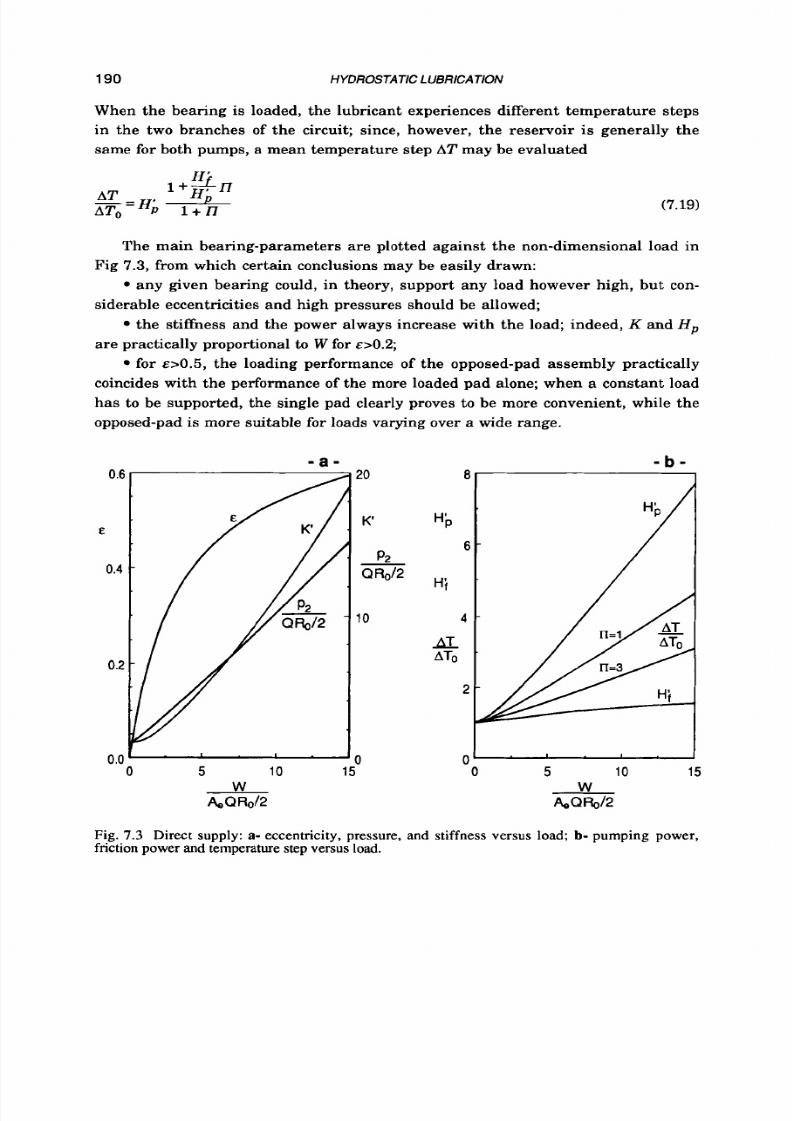
8/9/2019 Hydrostatic Lubrication 1992
http://slidepdf.com/reader/full/hydrostatic-lubrication-1992 207/558
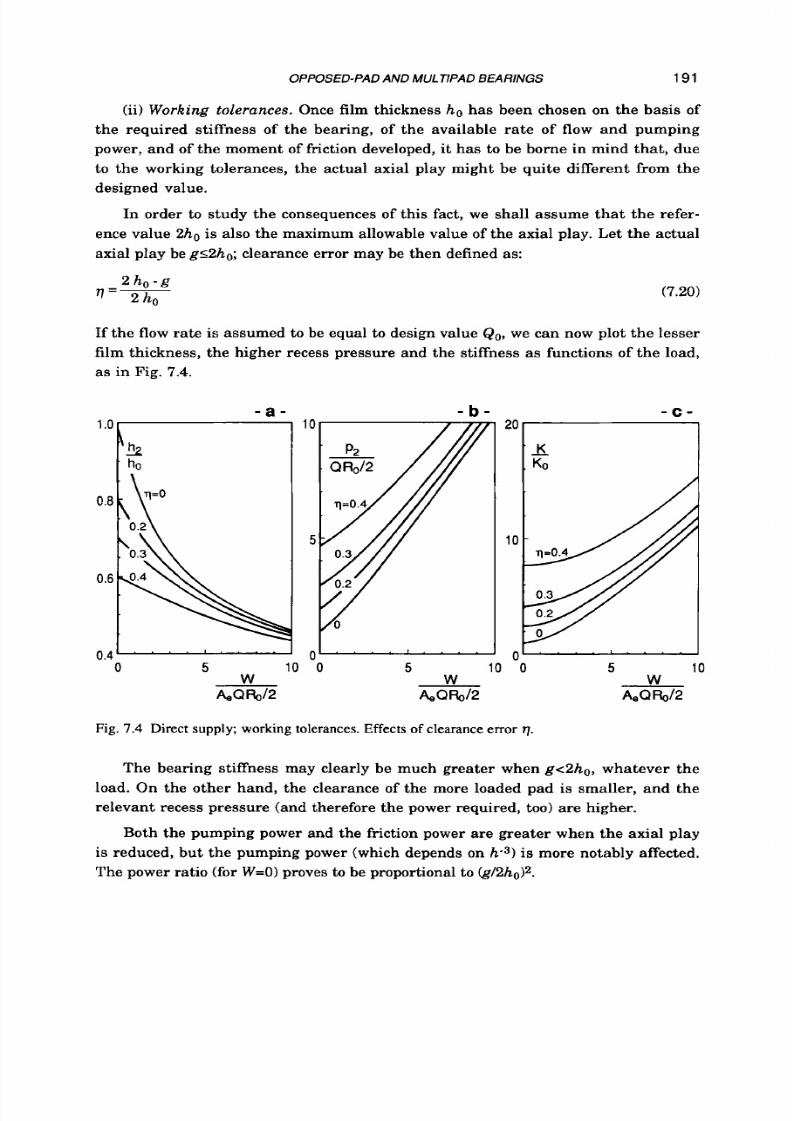
8/9/2019 Hydrostatic Lubrication 1992
http://slidepdf.com/reader/full/hydrostatic-lubrication-1992 208/558
OPPOSED-PAD AND MUL TIPAD BEARINGS
191
(ii) Working tolerances. Once film thickness
ho
has been chosen on the basis of
the required stiffness of the bearing, of the available rate of flow and pumping
power, and of the moment of friction developed, it has to be borne in mind that, due
to the working tolerances, the actual axial play might be quite different from the
designed value.
In order to study the consequences of this fact, we shall assume th at the refer-
ence value
2ho
is also the maximum allowable value of the axial play. Let the actual
axial play be
g12ho;
clearance error may be then defined as:
(7.20)
If the flow rate is assumed to be equal to design value
Qo,
we can now plot the lesser
film thickness, the higher recess pressure and the stiffness as functions of the load,
as in Fig. 7.4.
- a -
- b -
0.4' ' ' ' '
'
' ' . .
0
5 10
0
5
10
-0
5
10
W
W
W
& Q W
&QRo/2
A,Q Fb/2
Fig. 7.4 Direct supply; working tolerances. Effects of clearance error q.
The bearing stiffness may clearly be much greater when
g c 2 h o ,
whatever the
load. On the other hand, the clearance of the more loaded pad is smaller, and the
relevant recess pressure (and therefore the power required, too) are higher.
Both the pumping power and the friction power are greater when the axial play
is reduced, but the pumping power (which depends on
h-3)
is more notably affected.
The power ratio (for W=O)proves to be proportional t o (g/2ho)2.
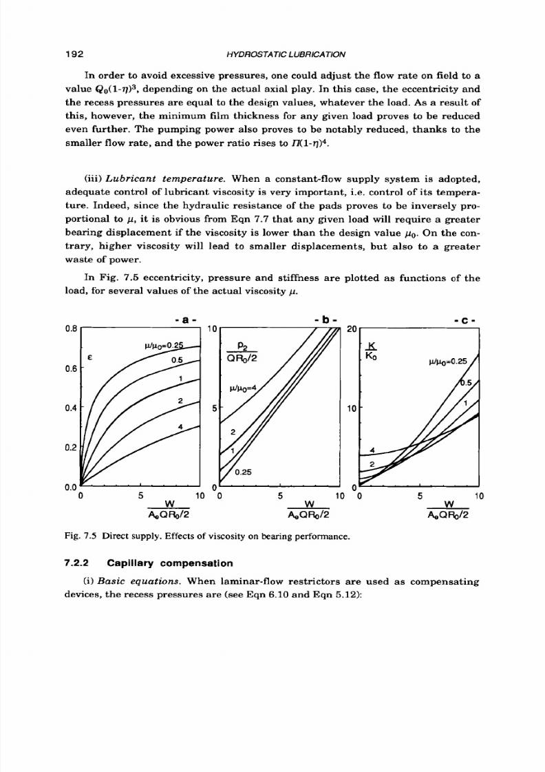
8/9/2019 Hydrostatic Lubrication 1992
http://slidepdf.com/reader/full/hydrostatic-lubrication-1992 209/558
192 HYDROSTATIC LUBRICATION
In order to avoid excessive pressures, one could adjust the flow rate on field to a
value
Q0(l -9)3 ,
depending on the actual axial play. In this case, the eccentricity and
the recess pressures are equal to the design values, whatever the load. A s a result of
this, however, the minimum film thickness for any given load proves to be reduced
even further. The pumping power also proves
t o
be notably reduced, thanks t o the
smaller flow rate, and the power ratio rises to I7( l-q)?
(iii)
Lubricant temperature.
When a constant-flow supply system is adopted,
adequate control of lubricant viscosity is very important, i.e. control of its tempera-
ture. Indeed, since the hydraulic resistance of the pads proves to be inversely pro-
portional
to p,
t is obvious from Eqn 7.7 that any given load will require a greater
bearing displacement if the viscosity is lower than the design value
po.
On the con-
trary, higher viscosity will lead
t o
smaller displacements, but also to a greater
waste of power.
In Fig.
7.5
eccentricity, pressure and stiffness are plotted as functions of the
load, for several values of the actual viscosity p.
- b - - C -
20
10
0
0
5 10
-0
5 10
-0
5 10
W W
W
&,Q5/2
&gab/: & Q 5 / 2
Fig.
7.5 Direct supply. Effects of
viscosity
on bearingperformance.
7.2.2
Capi l lary compensat ion
(i)Basic equations. When laminar-flow restrictors are used
as
compensating
devices, the recess pressures are (see Eqn 6.10 and Eqn 5.12):
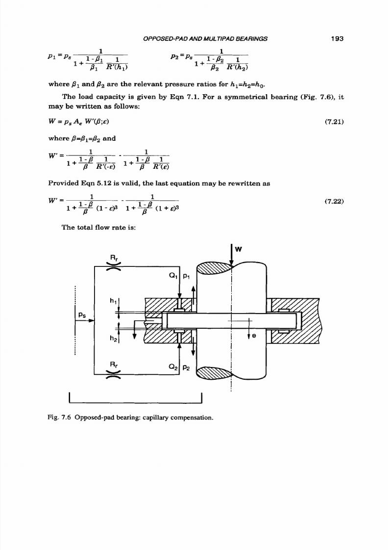
8/9/2019 Hydrostatic Lubrication 1992
http://slidepdf.com/reader/full/hydrostatic-lubrication-1992 210/558
193
where
P1
and
P2
are the relevant pressure ratios for h1=h2=h0.
The load capacity is given by Eqn 7.1. For a symmetrical bearing (Fig. 7.61, it
may be written as follows:
W
=
ps
A, Wc(1;~)
where
p=P1=p2
nd
W' =
(7.21)
1
1
R ' ( 4
P
RYE)
1 - 1 3 1
l uL
Provided Eqn 5.12
is
valid, the last equation may be rewritten as
The total flow rate is:
(7.22)
Fig. 7.6 Opposed-pad bearing: capillary compensation.

8/9/2019 Hydrostatic Lubrication 1992
http://slidepdf.com/reader/full/hydrostatic-lubrication-1992 211/558
194
HYDROSTATIC LUBRlCATlON
- a -
0.6
0.8
1
o
w
A,
Ps
- b -
0.6
0.5
0.0I.... ....
0.0 0.5
1 o 0.0
0.5
1
o
Ae PS Ae
PS
Fig.
7.7
Capillary compensation:
a-
eccentricity, b-
flow
rate and c- stiffness versus load, for
certain values of the pressure ratio.

8/9/2019 Hydrostatic Lubrication 1992
http://slidepdf.com/reader/full/hydrostatic-lubrication-1992 212/558
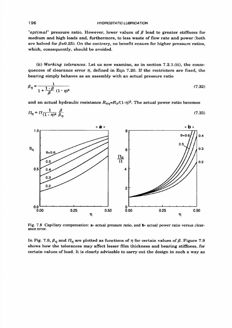
8/9/2019 Hydrostatic Lubrication 1992
http://slidepdf.com/reader/full/hydrostatic-lubrication-1992 213/558
196 HYDROSTATIC LUBRICATION
"opt imal"pressure ratio. However, lower values of
p
lead to greater stiffness for
medium and high loads and, furthermore,
to
less waste of flow
rate
and power (both
are halved for p=0.25). On the contrary, no benefit ensues for higher pressure ratios,
which, consequently, should be avoided.
(ii)
Working
tolerances. Let us now examine, as in section 7.2.1.W, the conse-
quences of clearance error q , defined in Eqn 7.20. If the restrictors are fixed, the
bearing simply behaves as an assembly with an actual pressure ratio
1
1+
(1 q ) 3
Bq =
(7.32)
and an actual hydraulic resistance R o q = R 0 / ( l - q ) 3 .he actual power ratio becomes
- a -
1
(7.33)
- b -
8
6 -
n
4 -
0.4
0.3
0.2
6.00
0.25 0.50
rl
Fig.
7.8
Capillary compensation:
a-
actual pressure ratio, and
b-
actual power ratio versus clear-
ance error.
In Fig. 7.8,
pq
and l7,,are plotted as functions of q for certain values of p . Figure 7.9
shows how the tolerances may affect lesser film thickness and bearing stiffness, for
certain values of load. It is clearly advisable to carry out the design in such a way as

8/9/2019 Hydrostatic Lubrication 1992
http://slidepdf.com/reader/full/hydrostatic-lubrication-1992 214/558

8/9/2019 Hydrostatic Lubrication 1992
http://slidepdf.com/reader/full/hydrostatic-lubrication-1992 215/558
198
HYDROSTATIC LUBRICATION
the flow rate (Eqn 4.76).With the help of the results obtained in sect. 6.3.2, it is pos-
sible t o obtain a set of equations describing the static behaviour of such bearing
systems.
For a symmetrical bearing, the load capacity may be written in the form of Eqn
7.21, but W now stands for the more complicated equation
1
w’=2[l+
- 1 + 4+1 + 4
p2
(1 + &)6 ]
(7.34)
In the same way, the total flow rate, the pumping power, the friction power, the
power ratio and the temperature step are given by Eqn 7.23, Eqn 7.28, Eqn 7.12, Eqn
7.29
and Eqn
7.30,
respectively, in which
Q’
stands for the following equation:
(1
+
&)3
+
1 - &)3
&’=
l + + q z - 1 + 4 +
Bearing stiffness may still be put in the form of Eqn 7.25, where
(7.35)
(7.36)
(1 + &)5
+
4- [
++ q G z 1”
(7-37)
The main parameters are plotted against the load in Fig.
7.10.
It
is easy
t o
see
that the orifices yield greater stiffness than the capillaries (the maximum stiffness
is now obtained for
p=0.586).
(ii) Lubricant temperature and working tolerances. One drawback to orifices is
that the system now proves
to
be highly sensitive to the viscosity
of
the lubricant,
which directly affects stiffness and load capacity.
If /3 is the design value of the pressure ratio for design axial play 2ho and viscos-
ity
p o ,
the actual pressure ratio p,, proves to depend on the clearance error q and on
the actual value of viscosity p:

8/9/2019 Hydrostatic Lubrication 1992
http://slidepdf.com/reader/full/hydrostatic-lubrication-1992 216/558
OPPOSED-PA D AND MULTIPAD BEARINGS 199
- a -
0.0 0.2 0.4
0.6
0.8
1
o
- b -
0.5
0.4
w
Ae
PS
- c -
0.0'
. . ' . ' . . . '
0.0 0.5 1 o
0.0
0.5 1 o
w
Jv
Ae PS Ae PS
Fig.
7.10
Orifice compensation:
a-
eccentricity,
b- flow
rate and c- stiffness versus load, for
certain values of the pressure ratio.

8/9/2019 Hydrostatic Lubrication 1992
http://slidepdf.com/reader/full/hydrostatic-lubrication-1992 217/558
200
HYDROSTATIC LUBRlCATlON
- a -
1 C
h
0.5
0.C
C
15
?l
n
10
5
- b -
1 0.25 0.50 0.00 0.25
0.50
1 (1-v m 11
Fig. 7.11 Orifice compensation. Effects of clearance error and lubricant viscosity on: a- pressure
ratio; b- power ratio.
- a -
1 o
- =0.3&,P,
K
2
..
1
- b -
r
0 1 . ’
” ’ . . ‘ .
0.00 0.25
0.50
11
Fig.
7.12 Orifice compensation . Effects of clearance error and lubricant viscosity
on:
a-
lesser film
thickness; b- stiffness.
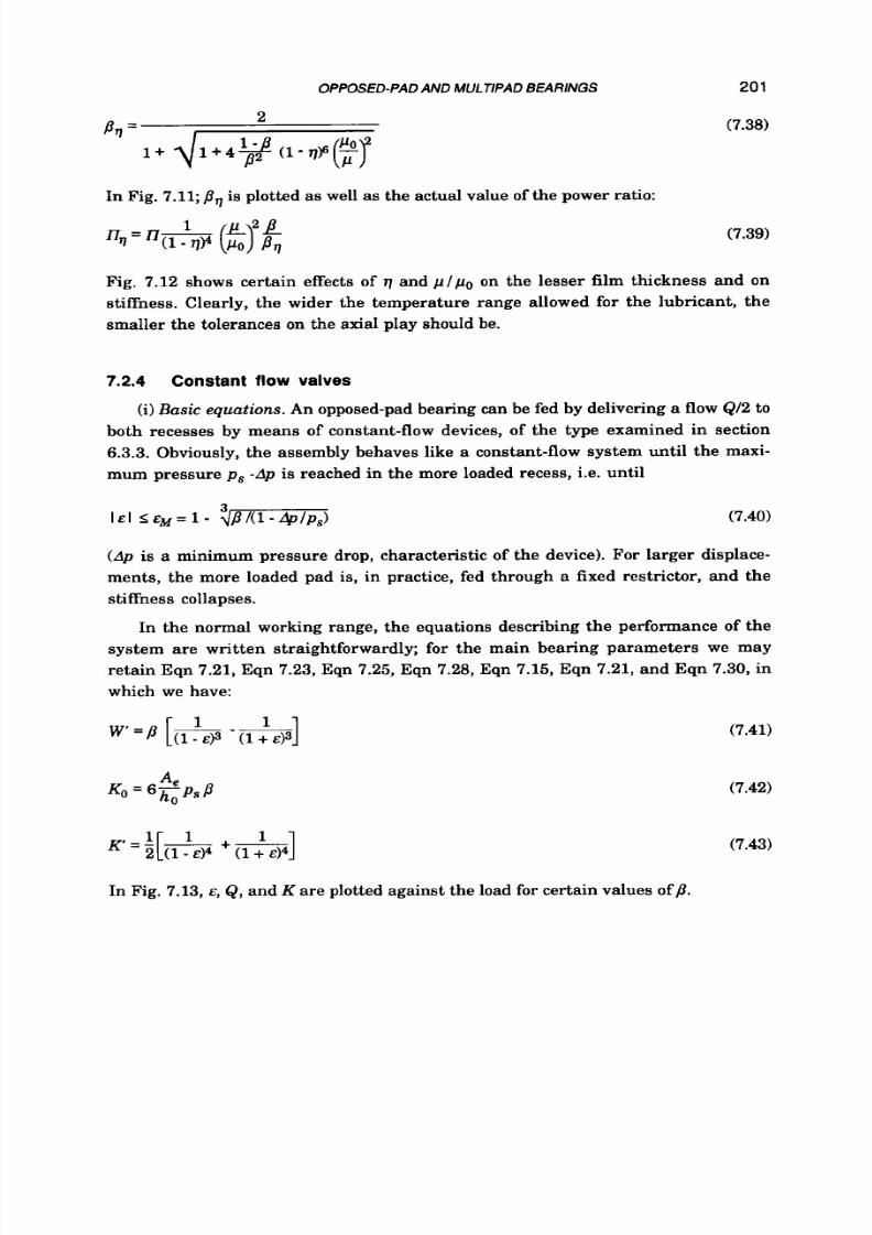
8/9/2019 Hydrostatic Lubrication 1992
http://slidepdf.com/reader/full/hydrostatic-lubrication-1992 218/558
OPPOSED-PAD AND MULTIPAD BEARINGS
2
a m =
In Fig.
7.11;Pq
is plotted as well as the actual value of the power ratio:
20
1
(7.38)
(7.39)
Fig.
7.12
shows certain effects of
7
nd p / p 0 on the lesser film thickness and on
stiffness. Clearly, the wider the temperature range allowed
for
the lubricant, the
smaller the tolerances on the axial play should be.
7.2.4 Constant f l ow valves
(i)Basic equations. An opposed-pad bearing can be fed by delivering a flow
Q/2
to
both recesses by means of constant-flow devices, of the type examined in section
6.3.3.
Obviously, the assembly behaves like a constant-flow system until the maxi-
mum pressure p s -Ap is reached in the more loaded recess, i.e. until
(7.40)
I& lI f = l -
3/(l-.4p/ps)
(Ap
is
a minimum pressure drop, characteristic of the device). For larger displace-
ments, the more loaded pad is, in practice, fed through a fixed restrictor, and the
stiffness collapses.
In the normal working range, the equations describing the performance of the
system are written straightforwardly; for the main bearing parameters we may
retain Eqn
7.21,
Eqn
7.23,
Eqn
7.25,
Eqn
7.28,
Eqn
7.15,
Eqn
7.21,
and Eqn
7.30,
in
which we have:
1 1
w ' = p
[m
(7.41)
(7.42)
(7.43)
In Fig.
7.13,
E,
Q,
and
K
are plotted against the load for certain values of j3.

8/9/2019 Hydrostatic Lubrication 1992
http://slidepdf.com/reader/full/hydrostatic-lubrication-1992 219/558
202
HYDROSTATIC LUB RICATlON
- a -
0.0'
' ' . .
'
'
0.6
0.8
1
o
W
-
A, Ps
0.0
0.5 1
o 0.0 0.5
1
o
W
-
-
A, Ps A, Ps
Fig.
7 .13
Constant-flow values: a- eccentricity, b- flow rate and c- stiffness of the bearing
versus load, for certain values
of
the pressure ratio and Ap/p,=O.I.

8/9/2019 Hydrostatic Lubrication 1992
http://slidepdf.com/reader/full/hydrostatic-lubrication-1992 220/558
OPPOSED-PAD AND MULTIPAD B EARINGS 203
(ii) Working tolerances. Let us now consider the effect of the working tolerances.
If the axial play g is a fraction
(1-9)
of design value 2h0, the actual hydraulic resis-
tance of the pad clearances becomes Roq=Ro/(l-q)3 nd hence the actual pressure
ratio rises to
p,=p/(
1-9)s.
The main consequences are:
stiffness increases: e.g. K(W=O)proves t o be proportional to
V(1-9);
on the other hand, the load range + W ( E M ) ,n which both the feeding devices act
correctly, is reduced (substitute
pq
fo rp in Eqn 7.40) as shown in
Fig.
7.14;
friction power and power ratio a re proportional t o 1/(1-9).
- a -
n
v .v
0.00
0.25 0.50
n
Fig. 7.14
Constant-flow valves: maximum displacement and relevant load versus clearance error,
for certain values of the pressure ratio and Apip,=O.l.
Clearly, narrow tolerances and small pressure ratios are required to ensure
high load-capacity; thus, the designer may not make the most of the potentiality of
such a supply system; furthermore, the stiffness of the actual system would be
much higher than necessary. This kind of problem may be overcome by planning
for an on-field adjustment of the flow rates delivered by the valves, in such a way as
to restore the planned pressure ratio whatever the actual value
of
the play
is: i.e.
the total flow rate must be Q(l-9I3 nstead of Q. n
this
way, a n error concerning the
play no longer affects load capacity. Stiffness in the unloaded configuration
is
now
proportional
t o l/(l-q).
The friction power is also proportional to
l/(l-q),
whereas the
power ratio becomes
nq=n/(l-q)4.

8/9/2019 Hydrostatic Lubrication 1992
http://slidepdf.com/reader/full/hydrostatic-lubrication-1992 221/558
204
HYDROSTATIC LUBRICATION
(iii) Lubricant temperature. The effect of a change in lubricant viscosity
is, of
course, connected with the behaviour of the flow-control valve.
It
has been already
noted that the "ideal" device (for this kind of application) should be able to provide a
flow rate that is independent from recess pressure, but inversely proportional
t o
lubricant viscosity. In this case, the loading performance of the system would not be
affected, while the pumping and friction powers would be proportional to l / p and t o
p, espectively. A
"true"
constant flow valve, on the other hand, provides the same
flow rate, whatever lubricant viscosity is. The main consequences are very similar
to those already seen in the case of the bearings directly fed by positive-displacement
pumps; in particular, the actual pressure ratio is proportional to p, thus a warmer
lubricant leads to less stiffness, while a cooler lubricant leads to greater stiffness,
counterbalanced by a narrower load-range (it is easy to see, from the equations
above, that if viscosity is too high, the valves cannot deliver the flow rate planned,
even
at
W=O ).
7.2.5
Flow dividers
(i)
Basic equations. Flow dividers may be used
to
improve the performance of the
opposed-pad bearings, as compared to the fixed-restrictor supply systems. Some of
these devices are introduced in section 2.3.2.
To s ta rt with, let us consider the
cylindrical-spool valve
in Fig.
2.13.
The hy-
draulic resistance
of
the two branches of the device depends directly on the dis-
placement x of the spool:
(7.44)
The displacement in its turn depends on the recess pressures, i.e. on the load. In
non-dimensional form it may be written as follows
(7.45)
Bearing in mind Eqn
7.2
and Eqn
7.21;
displacement may be rewritten
as
follows:
<=-'-A
i o K u ps w'
(7.46)
Since we have
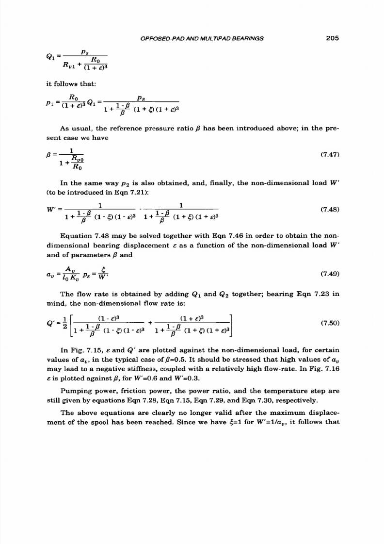
8/9/2019 Hydrostatic Lubrication 1992
http://slidepdf.com/reader/full/hydrostatic-lubrication-1992 222/558
OPPOSED-PAD AND MULTIPAD BEA RINGS
205
it follows that:
As
usual, the reference pressure ratio p has been introduced above; in the pre-
sent case we have
(7.47)
In the same way
p 2 is
also obtained, and, finally, the non-dimensional load W'
(to be introduced in Eqn 7.21):
(7.48)
Equation
7.48
may be solved together with Eqn
7.46
in order
t o
obtain the non-
dimensional bearing displacement
E
as a function of the non-dimensional load
W'
and of parameters p and
A , 5
a,
=-
lo K, p S =
w'
(7.49)
The flow rate is obtained by adding Q1 nd
Q2
together; bearing Eqn 7.23 in
mind, the non-dimensional flow rate is:
(7.50)
In
Fig.
7.15, E
and
Q'
are plotted against the non-dimensional load, for certain
values of
a,,
n the typical case of p=O.5. It should be stressed th at high values of a,,
may lead
t o
a negative stiffness, coupled with a relatively high flow-rate. In Fig. 7.16
E is plotted against p, for W=0.6and W=0.3.
Pumping power, friction power, the power ratio, and the temperature step are
still given by equations Eqn
7.28,
Eqn
7.15,
Eqn
7.29,
and Eqn
7.30,
respectively.
The above equations are clearly no longer valid after the maximum displace-
ment of the spool has been reached. Since we have {=1 for W'=lla,,
it
follows that
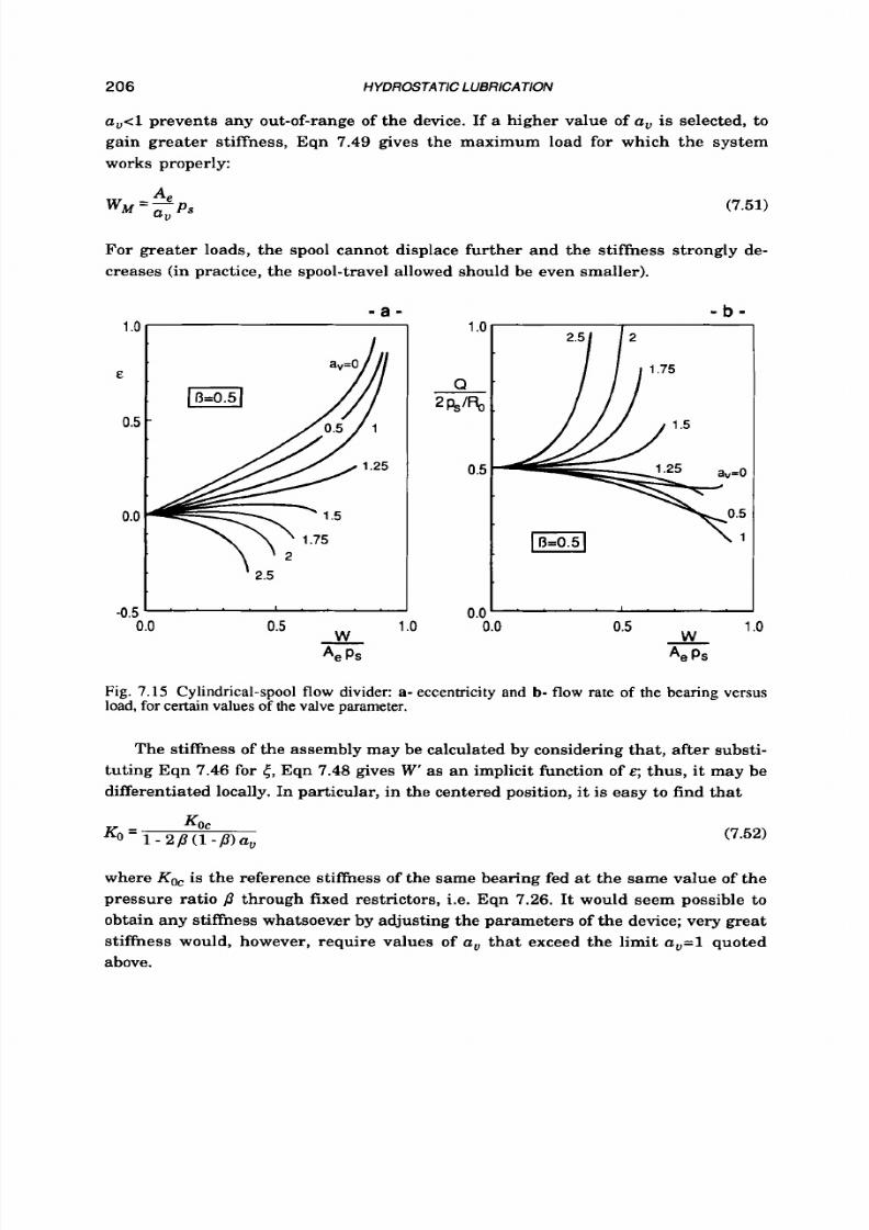
8/9/2019 Hydrostatic Lubrication 1992
http://slidepdf.com/reader/full/hydrostatic-lubrication-1992 223/558
206 HYDROSTATIC LUBRICA TlON
a,<l prevents any out-of-range of the device. If a higher value of a, is selected, to
gain greater stiffness, Eqn 7.49 gives the maximum load for which the system
works properly:
A
w
M - a ,
e p s
(7.51)
For greater loads, the spool cannot displace further and the stiffness strongly de-
creases (in practice, the spool-travel allowed should be even smaller).
- a -
- b -
1 . 0 1 I
1
o
Q
2k'
0.5
0.0
0.0
0.5
1 o 0.0
0.5
1
o
W
- -
A e PS Ae PS
Fig. 7.15 Cylindrical-spool flow divider: a- eccentricity and
b-
flow rate of the bearing versus
load,
for
certain values
of
the valve parameter.
The stiffness of the assembly may be calculated by considering that , after substi-
tuting Eqn
7.46
for 5, Eqn
7.48
gives
W'
as an implicit function of
E;
thus, i t may be
differentiated locally. In particular, in
t h e
centered position, it is easy to find that
(7.52)
where Koc is the reference stifmess of the same bearing fed a t the same value of the
pressure ratio p through fixed restrictors, i.e. Eqn 7.26. t would seem possible to
obtain any stiffness whatsoever by adjusting the parameters of the device; very great
stiffness would, however, require values of a,, hat exceed the limit
aU=1
uoted
above.

8/9/2019 Hydrostatic Lubrication 1992
http://slidepdf.com/reader/full/hydrostatic-lubrication-1992 224/558
OPPOSED-PAD AND MULTlPAD BEA RINGS
207
Better performances may be obtained with the
tapered-spool value
in Fig. 2.14.
The hydraulic resistances of the two branches
of
the device may be expressed in the
following form:
0.d
E
0.
- a -
(7.53)
- b -
0.1
0.0
0.5 1
o
0
0.0 0.5 1 o
B
Fig.
7.16 Cylindrical-spool flow divider: eccentricity of the bearing versus pressure ratio,
for
cer-
tain values
of
the valve parameter.
The position
of
the spool depends on the load, according to Eqn 7.46. Proceeding
as
before, we again obtain Eqn 7.21 and Eqn 7.23, in which:
1
(7.54)
'=
1

8/9/2019 Hydrostatic Lubrication 1992
http://slidepdf.com/reader/full/hydrostatic-lubrication-1992 225/558
208 HYDROSTATIC LUBRlCATfON
- a -
1.01
0.0
0.5
1o
-
A, PS
1 a
Q
-
24’%
0.5
0.c
I
- b -
1 o
w
A, PS
0.5
Fig.
7.17 Tapered-spool flow divider:
a-
eccentricity and b- flow rate of the bearing versus load,
forcertain values of the valve parameter.
- a -
0.E
E
0.4
0.C
I
I3
- b -
0.5 1
o
I3
Fig. 7.18 Tapered-spool flow divider: eccentricity of the bearing versus pressure ratio, for certain
values
of
the valve parameter.
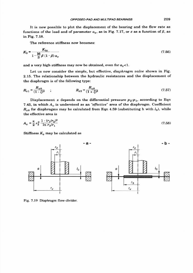
8/9/2019 Hydrostatic Lubrication 1992
http://slidepdf.com/reader/full/hydrostatic-lubrication-1992 226/558
OPPOSED-PAD AND MUlTlP AD BEA RINGS
209
It
is now possible to plot the displacement of the bearing and the flow
rate
as
functions of the load and of parameter
a , ,
as in Fig. 7.17,
o r
E as a function
of 8 ,
as
in Fig. 7.18.
The reference stiffness now becomes:
and a very high stiffness may now be obtained, even for a,<l.
Let us now consider the simple, but effective,
diaphragm
v a lv e shown in Fig.
2.15. The relationship between the hydraulic resistances and the displacement of
the diaphragm
is
of
the following type:
Displacement
x
depends on the differential pressure
p 2 - p l ,
according to Eqn
7.45, in which A, is understood as a n "effective"area of the diaphragm. Coefficient
RvO
or diaphragms may be calculated from Eqn
4.59
(substituting h with l o ) , while
the effective area is
(7.58)
Stiffness K , may be calculated as
- b -
r2
I
I
Fig. 7.19 Diaphragm flow-divider.

8/9/2019 Hydrostatic Lubrication 1992
http://slidepdf.com/reader/full/hydrostatic-lubrication-1992 227/558
210 HYDROSTATIC LUBRICA TlON
(7.59)
for diaphragms as in Fig.
7.19.b,
whereas for diaphragms
as
in Fig.
7.19.a
he fol-
lowing may be taken:
(7.60)
Proceeding as above, the non-dimensional load and
flow
rate are easily found
(see also Fig.
7.20
and Fig.
7.21):
1
1
- a -
1 . 0 r I
(7.61)
(7.62)
- b -
1
.o
w
*e
PS PS
0.0 0.5 1 o 0.0
0.5
-
Fig.
7.20
Diaphragm flow-divider:
a-
eccentricity and
b-
flow rate
of
the
bearing
versus load, for
certain
values
of the valve parameter.
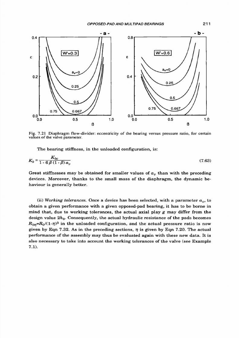
8/9/2019 Hydrostatic Lubrication 1992
http://slidepdf.com/reader/full/hydrostatic-lubrication-1992 228/558
OPPOSED-PAD AND MUL TIPAD BEA RINGS
211
- a -
0.4
E
0.:
0.1
- b -
0.8 I
E
0.4
0.0
0.5
1
o 0.0
0.5 1
o
D D
Fig. 7.21 Diaphragm flow-divider: eccentricity of the bearing versus pressure ratio, for certain
values
of
the valve parameter.
The bearing stiffness, in the unloaded configuration,
is:
(7.63)
Great stiffnesses may be obtained for smaller values of
a,
than with th e preceding
devices. Moreover, thanks
t o
the small mass of the diaphragm, the dynamic be-
haviour is generally better.
(ii)
Workin g tolerances.
Once a device has been selected, with a parameter
a,,
to
obtain a given performance with a given opposed-pad bearing, it has to be borne in
mind that, due to working tolerances, the actual axial play g may differ from the
design value
2 4 .
Consequently, the actual hydraulic resistance of the pads becomes
Roq=RoI(l-q)3n the unloaded configuration, and the actual pressure ratio is now
given by Eqn 7.32.
As
in the preceding sections, q is given by Eqn
7.20.
The actual
performance of the assembly may thus be evaluated again with these new data. I t is
also necessary to take into account the working tolerances of the valve (see Example
7.1).
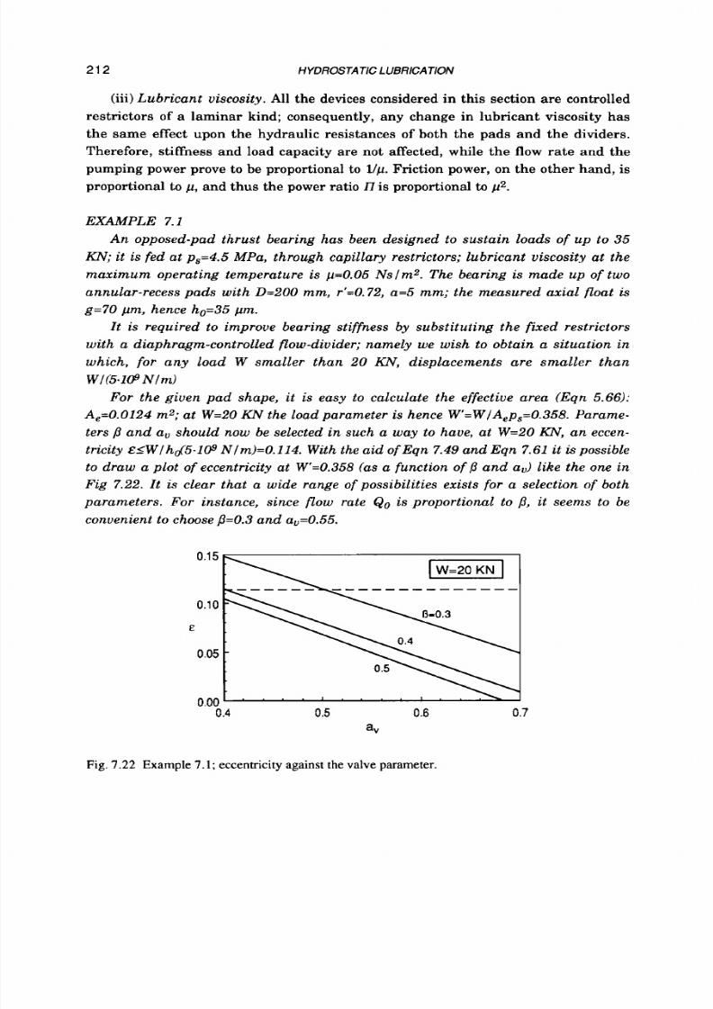
8/9/2019 Hydrostatic Lubrication 1992
http://slidepdf.com/reader/full/hydrostatic-lubrication-1992 229/558
8/9/2019 Hydrostatic Lubrication 1992
http://slidepdf.com/reader/full/hydrostatic-lubrication-1992 230/558
OPPOSED-PAD AND MU1TlPAD BEARINGS
21
3
Of course, it is necessary to also verify the behaviour of the system for different
loads. For small loads, Eqn 7.63 gives K0=3.26.K,=6.5S.1@ N l m (bear in mind that
KO, s the stiffness tallying to simple capillary restrictors, Eqn 7.26), which is much
higher than required. At the maximum load W=35
K N
(i.e. W'=0.626), eccentricity
may be calculated as ~=0.22, good result compared with capillary compensation.
Flow rate at W=O can be easily calculated: for p=0.05 Nslm2, &0=41.7.10-6m3/s.
The relevant pumping power is, hence, Hp0=188
W.
Equation 7.62 shows that Q and
H p are smaller when the bearing is loaded.
Concerning the design of the controlled restrictor, the reader should verify that
the selected value of the pressure ratio may be obtained (for instance) with r2=6 mm,
r,=3 mm, and 10=76 pm (see Fig. 7.19) and that the relevant Reynolds number is
quite low. Parameter A, is easily calculated: A,=0.061~10-3m2. From Eqn 7.49 it
follows that the stiffnessof the diaphragm should be K,=6.59.106 N l m; for instance,
using a steel diaphragm (El(l-v2)=226GPa) with a thickness s=l mm, the required
value of K, may be obtained selecting rv=12.6 mm, for the diaphragm in Fig. 7.19.a.
It is clear that the designed values of a, and
jl
can only be obtained with a cer-
tain approximation, but
they are not critical, in this case, since limited variations
can be allowed, as may be seen by examining Fig. 7.22. In particular, it may seem
difficult to obtain exactly the calculated value of clearance lo; nevertheless a greater
clearance would clearly lead to quite small changes in stiffness,
For
instance, to
increase
lo
by
20%
would give av=0.458 and /3=0.425, and hence the displacement at
W=20
KN
remains practically unchanged. Of course, flow rate would increase as
the pressure ratio increases.
7.2.6
Design
of
opposed-pad bear ings
In most cases the specifications of thrust bearings consist in a certain value
W,
of the load to be sustained a t a displacement smaller than a certain value eM. Cer-
tain obvious constraints generally exist for the size of the bearing, a s well as for the
supply system (max. pressure and flow rate; viscosity of the lubricant) and for the
friction (max. torque).
Since
too
many parameters and constraints are involved, a general design pro-
cedure cannot be given, except
for
certain main aspects: let
us
briefly examine how
the choices of the designer may affect the final result, and try t o assess optimal
values of certain parameters, on the usual basis of the least power loss. For the sake
of brevity, the following considerations will refer mainly to the case of annu-
lar-recess pads fed through laminar-flow restrictors, but they could easily be ex-
tended
to
other pad shapes and supply systems.
A s
a
first
design step, one may
try
to select
a
maximum value
EM
of the eccen-
tricity, commonly & ~=0 . 5 ;owever, it
is
not advisable t o allow eccentricities greater
8/9/2019 Hydrostatic Lubrication 1992
http://slidepdf.com/reader/full/hydrostatic-lubrication-1992 231/558
21
4 HYDROSTATIC LUBRICATlON
than 0.6. When a maximum value of the displacement is given, this immediately
leads to an upper constraint
gk=2
eM/&M for the axial play
g=2ho.
When high stiff-
ness is required, g),,may prove to be too small; in this case i t may be useful to select a
smaller value for the eccentricity.
A
set of geometrical parameters can now be stated: as for the single-pad bear-
ings, it is generally convenient to select large lands for low-speed bearings, the con-
trary for high-speed bearings.
The pressure ratio should remain in the 0.3+0.6 range; it is advisable
to
start
fixing a low value for the design pressure ratio j? in order to allow greater margins
for the working tolerances: this point is clarified below.
The load parameter
W ' ( E M $ ) = A ~ ,
an now be calculated, or read in the appro-
priate chart. Supply pressure is often prescribed, and then the effective pad area
(i.e. the pad size) is readily obtained; otherwise, both A, andp, have to be suitably
chosen. Caution is necessary in selecting high values for the supply pressure, since
an excessive temperature step in the lubricant may follow: see Eqn 7.30.
The problem of a suitable selection
of
the axial play and of the lubricant viscosity
may be tackled on the usual basis of minimization of the total power consumption:
Proceeding as in the case of the single-pad bearings (sect. 6.21, it may be found
that, for plane or tapered circular pads, rotating at a speed a, he total power may
be written as
the relevant value
of
the viscosity being
(7.64)
(7.65)
Equations for H; and
p i
are given in Chapter 6 (namely, Eqn 6.58 and Eqn 6.62; see
also Fig. 6.16 and Fig. 6.17). Equations 7.64 and 7.65 are valid for all constant-pres-
sure supply systems, provided the relevant values for W' are selected.
Examining Eqn
7.64, it
should be noted that,
as
for the single-pad bearings,
it
is
convenient to select large recesses and small clearances, provided that
a
lubricant
with sufficiently low viscosity is available, in order to get
n=1.
f, instead,
l
is
fixed,
the optimal value for axial play is the one which gives n=3.
8/9/2019 Hydrostatic Lubrication 1992
http://slidepdf.com/reader/full/hydrostatic-lubrication-1992 232/558
OPPOSED-PADAND MULTlPA D BEARINGS 215
Further observations are, however, necessary. In particular, i t must be stressed
that the choice of axial play is meaningless if the relevant working tolerances are
not specified. As a matter of fact, a whole range ( 2 h 0 - 6 ~ & < 2 h o should be selected,
instead of
a
single value, for the axial play
g.
To
reduce manufacturing costs,
it
is
advisable for tolerance
Sg
to be as large as possible, but i t has been shown th at large
tolerances can notably affect the performances of the bearing (e.g. see Fig. 7.8 and
Fig. 7 . 9 ) .For instance, selecting e ~ = 0 . 5 ,
3=0.5,
and
Sg=h0,
it may be seen that the
actual pressure ratio may prove t o be as great as 0.89 (take
q=0.5
in Eqn 7 . 3 2 ) ; he
main consequence is that load capacity is strongly reduced and the load designed t o
be sustained at
~ ~ = 0 . 5
annot be reached even at
e= l
(this may be verified by means
of Eqn 7 . 2 2 ) .It should therefore be clear that smaller tolerances must be selected.
The actual value of the power ratio will also be dependent on the actual clearance
(see Eqn 7 . 3 3 ) ; or instance, forfi=0.3, 6g=ho/1.5and
I7=1,
he actual power ratio may
prove t o be as great as 2.6.
A convenient design practice consists in first selecting a suitable value for toler-
ance
4;
xial play may then be chosen (e.g. with the aid of Eqn 7 . 3 2 ) n such a way
as
to
keep the actual pressure ratio within a reasonable range.
For
instance, we
may take
ho=l.6.6g
iffi=O.3,
or ho=2.2.6g
f/3=0.4. Smaller values for ratio ho/Sg can
be selected, when small eccentricities (e.g. ~ 0 . 3 )
re expected.
In order t o free the loading performances from the adverse effects of manufac-
turing tolerances, it is possible to select adjustable restrictors, that allow us to re-
store the design value of the pressure ratio on field, whatever the actual value
of
axial play. Nevertheless, for high-speed bearings, 6 should not be greater than h o / 2
to avoid excessive values of the power ratio. Instead, for low-speed bearings, toler-
ances may be larger.
Concerning viscosity of the lubricant,
it
should be borne in mind that, in gen-
eral, it may not be considered a constant, since it largely depends on lubricant
temperature, and hence on the working conditions and on the effectiveness of the
cooling of the reservoir. Unless a temperature control system is provided, it is ad-
visable to verify the performances of the bearing for all the expected range of viscos-
ity. In particular, when laminar-flow restrictors are used, f i is not affected by lubri-
cant temperature, nor load capacity. For low-speed bearings i t is convenient at the
design stage
t o
consider
p
as the lower end of the expected viscosity range (in this
way flow rate and power loss should always turn out to be smaller than calculated).
Otherwise, optimization may be looked for, for a center-of-range value of viscosity: it
is then necessary to check flow rate and power for all the viscosity range
(it
is con-
venient, however, for the supply system to be able to keep lubricant temperature
within a narrow range).
8/9/2019 Hydrostatic Lubrication 1992
http://slidepdf.com/reader/full/hydrostatic-lubrication-1992 233/558
21
6 HYDROSTATIC LUBRICATION
A s a result of the above remarks, a simple procedure may be proposed that
should lead to a quick and "optimized"design of the opposed-pad bearings. Let us
assume a certain load W M s given, to be sustained with a displacement smaller
than
e M ;
urther constraints may be required (e.g. viscosity
o r
supply pressure may
be imposed): the device may then be designed following the steps listed below.
i)
Choose a trial set of geometric parameters: select large recesses unless low
speeds are expected.
Choose a trial value of the maximum eccentricity, such as ~ ~ = 0 . 5 .
Choose a trial value of the design pressure ratio: perhaps p=0.3.
ii) Evaluate coefficient W' (e.g. from Eqn 7.22, for capillary compensation).
Decide supply pressure
p s ,
when it is not prescribed, and effective area A,,
in such
a
way
to
satisfy Eqn
7.21.
Calculate the pad size, in order to get the above value ofA,.
iii) Select a suitable value for the manufacturing tolerance on axial play: bear in
mind that the narrower
Sg
is, the lower the power losses can be.
Select the design film thickness ho (the actual value
g
of the axial play must
consequently lie in the 2hot2ho-Sg range); for capillary compensation, it
should be
ho>1.5.Sg;
smaller values may be used if ~ ~ c 0 . 5 ,ut wider clear-
ance should be selected for p>0.3.
Check if stiffness is large enough (Eqn
7.26,
for capillary compensation).
Otherwise reduce Sg and ho, or select a smaller value for EM, starting again
from point (ii),
iv) Calculate the
"optimal"
value of viscosity, i.e. the value k p t that leads to
l7=1
(e.g. by means of Eqn 7.65, for rotating thrust-bearings).
Check that
b p t
is a plausible value (sometimes p may be directly imposed by
the specifications);
if
it is not, try
t o
modify the geometrical parameters
(namely the recess width) or the design film thickness
or
the supply pres-
sure. However, if the speed is very low, it will not be possible to get
n=1;
n
this case select the highest allowable viscosity, and the recess width that
ensures the least consumption of pumping power. On the contrary, a very
high speed would lead t o values for b p t which are too small; in this case
it
is
necessary to accept values of l7 greater than 1.
v) Calculate flow rate (Eqn 7.231, pumping power (Eqn 7.281, friction force (or
friction torque) and friction power (Eqn 7.15), with reference to the design
configuration @=hotE=O).
Check the same parameters for different values of play and eccentricity.
Should flow rate seem
too
great, and
h o
cannot be further reduced, it will be
necessary t o accept a power ratio of l7>l (e.g. by increasing p
or
by reducing
8/9/2019 Hydrostatic Lubrication 1992
http://slidepdf.com/reader/full/hydrostatic-lubrication-1992 234/558
OPPOSED-PAD AND MULTIPAD BEA RINGS 217
ps ) , consequently increasing friction. Conversely, friction may be easily
reduced with a larger expenditure of flow rate and pumping power.
Check the temperature step in the lubricant (Eqn 7.30).
If the supply system is not able to keep lubricant viscosity within a narrow
range, check the friction and the temperature step for the maximum ex-
pected viscosity, too, and check the flow-rate for the minimum viscosity.
vi) Design the compensating restrictors (see section 4.7.6).
vii) Check the Reynolds number in the bearing clearances.
For bearings rotating at high speed, check the effect o f inertia forces in the
lubricant (see sections 5.3.4, 5.4.5 and
5.5.2).
viii) Check the dynamic behaviour
of
the system (see Chapter
10).
EXAMPLE 7.2
Design an annular-recess opposed-pad bearing to sustain a load varying in the
210
K N
range, with a stiffness that is always greater than 108 Nl m , and rotating at
157 radls (1500 rpm); the supply system to be
used
delivers lubricant at 7 MPa. Fur-
ther constraints consist in the inner pad diameter 2r, being required to be greater
or
equal to 45 mm and manufacturing tolerances to be in the order of 30
p
To start with, one may state the trial values for the pressure ratio (8=0.3) and for
the maximum eccentricity ( ~ ~ = 0 . 5 ) .ince laminar-flow restrictors are selected, the
load parameter is readily calculated (Eqn 7.22) as W=0.66; this means that a n effec-
tive area A, not smaller than 2.16.10-3 m2 is required (Eqn 7.21): for instance, D=72
mm, r’=O.625, and a=1.5 mm may be selected; hence Eqn 5.66gives A,=2.2.10-3 m2.
Since the value of tolerance on axial play is given, the maximum film thickness
can be selected: ho=1.5.&=45 pm; consequently the actual axial play g will be in the
60t90p range. From Eqn 6.62 we may obtain $=13.7; from Eqn 7.65 it follows that
a lubricant should be selected with a viscosity of p 0 . 3 Nslm2 n order to obtain
n=l.
From Eqn 5.68 and Eqn 5.72 we obtain Ro=161.109 Nslm5 and Hf0=87 W. The
calculations are now straightforward.
When g=2ho=90pm, stiffness at W=O is K0=O.43.1O9 N l m , flow rate is Q=26.10-6
m3/s,
pumping power and friction power are Hp=182 Wand Hf=175 W, respectively.
The design load can be sustained with an eccentricity that is slightly smaller than
0.5;
he relevant stiffness is again K=O.43.1O9 N l m (however, stiffness is greater for
intermediate loads); the flow rate and pumping power are smaller, while the fric-
tion power is 30% greater.
When g=2ho-fig=60 m, the actual pressure ratio becomes (Fig. 7.8) 8=0.59;
in
order to sustain 10
KN,
an eccentricity of ~ = 0 . 5 3s now required; the smallest film
thickness is therefore h,=14 pm. Stif fness at W=O is much greater than before
(K=O.75.1O9 Nlm), while at the maximum load
we
get K=O.41.1O9 N l m . The pump-

8/9/2019 Hydrostatic Lubrication 1992
http://slidepdf.com/reader/full/hydrostatic-lubrication-1992 235/558
218 HYDROS
JATlC LUBRICATION
ing power is obviously smaller; on the other hand, i t is Hf=262
W
a t W=O, nd
H f-365
W at W= 0 KN.
Th e hyd rau lic resistance of the restrictor m us t be Rr=Ro(l-p)p=376.1@N s l m 5 ;
this m ay be easily obtained, say, w ith a
1=30.75
mm
length o f a
1
mm -bore pipe.
The value of viscosity selected above may seem too high
in
certain ap plications.
It is clear th at to select a lower value would have no effect on bearing stif fness, but
flow rate and pumping power would become much greater.
For
instance, selecting
p=O.1 Nslrn2,
for
g=90 pm and
W=O
we would have
Hp=547 W
and
Hf-58 W ,
i.e.
I l = O . l ,
with a considerable increase
in
total power. In this case,
it
might prove
suitable t o slightly change the size
of
the pa d, increasing both
a
and
D
in order to
reduce H p .
7.3 LEAD
SCREWS
Hydrostatic lead screws may be treated, a t the beginning, in exactly the same
way as opposed-pad bearings, using the relevant values for
A,,
Ro, and
H f o
(see
section 5.10). Indeed it is possible to obtain the recessed nut by injection of resins,
using the treaded shaft itself as a mould (see. ref,
7.1);
his allows us to obtain pre-
cisely controlled values of axial play, and prevents large lead errors between screw
and nut, that may be responsible for a serious decline in performance, especially
when hydrostatic lubrication concerns several turns of the thread. However, the
pitch may not generally be considered to be constant for the whole length of the
screw, since local pitch variations exist, whose maximum value depends on the
degree of accuracy and overall length. Precision screws may show lead variations
in the order of 10+20 pm, although screws of even greater precision are commer-
cially available (ref. 7.2).
Let us now consider a nut working in a zone where the pitch of the threaded
shaft differs from the pitch of the nut by a quantity 6p; of course,
& is
meant
as
an
average error, since the pitch varies continuously. The main consequence is that
the available axial displacement between screw and nut is no longer
ho,
since con-
tact occurs at a n eccentricity
where we have introduced the non-dimensional pitch error
(7.66)
(7.67)
This fact may considerably reduce the load capacity of the system. Furthermore, the
hydraulic resistance of clearances no longer varies according to Eqn 5.12, as was
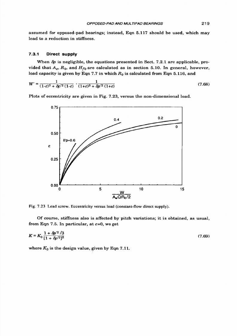
8/9/2019 Hydrostatic Lubrication 1992
http://slidepdf.com/reader/full/hydrostatic-lubrication-1992 236/558
OPPOSED-PAD AND MULTIPAD BEA RINGS
219
assumed for opposed-pad bearings; instead, Eqn
5.117
should be used, which may
lead
to
a reduction in stiffness.
7.3.1 Direct supply
When c5p is negligible, the equations presented in Sect. 7.2.1 are applicable, pro-
vided that A,, Ro, and H f o are calculated as in section
5.10.
In general, however,
load capacity is given by Eqn
7.7
in which Ro is calculated from Eqn
5.116,
and
(7.68)
1
w
=
( 1 4 3+
&i2 (I-&)
(1+43
+ &'2 (I+&)
Plots of eccentricity are given in Fig. 7.23, versus the non-dimensional load.
Fig.
7.23 Lead screw. Eccentricity versus
load (constant-flow
direct
supply).
Of course, stiffness also is affected by pitch variations; it is obtained, as usual,
from Eqn 7.5. In particular, at E=O,we get
(7.69)
where
KO s
the design value, given by Eqn
7.11.

8/9/2019 Hydrostatic Lubrication 1992
http://slidepdf.com/reader/full/hydrostatic-lubrication-1992 237/558
220
HYDROSTATIC LUBRICATION
7.3.2
Constant
pressure supply
flow rate , can be studied by substituting
R’=ll(l+d3
with
The effect of pitch errors on recess pressures, and then on load capacity and
(7.70)
For the sake of brevity, we shall discuss the results for only the simplest case,
i.e. capillary compensation, even
if
a new type of floating controlled restrictor (ref.
7.3)
has been proposed, especially for hydrostatic lead screws (ref.
7.4).
Load capac-
ity is obtained from Eqn
7.21,
where
(7.71)
In Fig 7.24 a plot of the load-eccentricity relationship is given for certain values of
the design pressure ratio and relative pitch error.
Flow ra te is still given by Eqn
7.23,
where
(7.72)
- a -
- b -
1
.I
E
O .
0
0
o
1
o
W
o 0.0
0.5
W
-
A e PS Ae PS
0.5
-
Fig.
7.24
Lead screw. Eccentricity versus
load
(constant-pressure supply, capillary restrictors).

8/9/2019 Hydrostatic Lubrication 1992
http://slidepdf.com/reader/full/hydrostatic-lubrication-1992 238/558
OPPOSED-PAD AND MULTIPAD BEA RINGS
221
Stiffness at
W=O
may be calculated by means of the following equation
(7.73)
where K O s given by Eqn 7.26.
In conclusion it may be noted that, to make manufacturing easier, the continu-
ous recess i s often substituted by a sequence of small pockets; in this case, the effec-
tive area (and hence the load capacity) is considerably reduced, but the hydraulic
resistance is greater: hence the flow rate is also reduced. If each pocket is fed inde-
pendently through a separate restrictor, the effect of the pitch error on load capac-
ity, flow rate, and stiffness is less pronounced than in the case of continuous recess
(see also ref.
7.5).
EXAMPLE 7.3
A hydrostatic lead screw has to carry loads as great as f 15 KN, with a rigidity
W / e greater than 109 Nl m , when supplied at a pressure ps=7 MPa; the friction
torque must be smaller than 5 N m at the maximum turning speed R=52 radls ( ~ 5 0 0
rpm). Moreover the overall length of the nut is required to be smaller than 200 m m
and its external diameter must be equal to 150 mm; the lead must be p*=20 mm.
Figure 7.24 shows that the product psA e must be substantially greater than the
maximum load W ~ = 1 5
N ;
initially, one may state that psAe>1.7.W~=25.5
N :
since ps is given, it follows that Ae23.64.10-3 m2. Let us select a thread with flank
angle 0=15 degrees, external diameter
D=90
mm and the root diameter of the nut
2r,=65 mm; taking a land width of 3.5 mm (i.e. a'=0.28) we get Az=0.34, and thus
lubrication should be extended to two turns o f the nut; indeed, introducing n=2 into
Eqn 5.115, it follows that A,=4.38.103 m2.
In order to properly select the design value of the fi lm thickness, it is necessary
to know the maximum value of the pitch error; assuming SpllO pm, it follows that
to obtain 6p'<0.4 we must have hO>%
pm
(Eqn 7.67). On the other hand, Fig. 7.24
shows that, assuming @=0.3,at the maximum load WM=15KN, we have an eccen-
tricity ~ 0 . 4 5for Sp3=0.4);hus, in order to have a displacement that is smaller than
e~=1 5.103/109 =15 pm, we must have h0133 pn . Finally, h0=30 pm may be cho-
sen. It is worth noting that i f the threaded shaft were built with greater accuracy, it
would be possible to select smaller values for h , with notable benefits in stiffness,
flow rate and pumping power.
Equation 5.71
(or
Fig. 5.14) gives HF=0.41 and then the friction power is (from
Eqn 7.15 and Eqn 5.118) Hf=(0.38 rn3).H;p@. The friction torque Mf=HfIRmustbe
smaller than
5
Nm: sincesat R=52 radl s and ~ = 0 . 4 5 i.e. Hj=1.25) it is
Mf=(25m31s).p, it follows that viscosity must be lower than 0.2 Nsl mz .

8/9/2019 Hydrostatic Lubrication 1992
http://slidepdf.com/reader/full/hydrostatic-lubrication-1992 239/558
222
HYDROSTATIC
LUBRlCA
TION
Th e flow rate depe nds on th e actual value o f viscosity (i.e.
it
is inversely propor-
tional to
it);
for instance,
if
we select p=O.l N sl m z, E qn 5 .116gives Ro=185.109 N sl m 5
and, hence, at W=O, Q=22.7.10-6
m3ls
and
Hp=159
W. Both th e f low rate and the
pum pin g pow er change lit t le wh en the load is applied.
The power loss due to friction at E=O and p=O.l N s l m z i s Hf=104 W a n d prov es to
be proportional to viscosity.
7.4
SELF-REGULATING BEARINGS
A self-regulating bearing (SRB) may be regarded as an opposed-pad bearing
with a built-in
flow
divider, which is made up of another couple of pads. Compared
to conventional flow dividers, however, the important advantage of the SRB, under
dynamic loading, is that
it
has no other moving part (such as spools o r di-
aphragms). On the other hand, the
"inf ini te st i f fness"
which could, in theory, be
achieved with the aforesaid devices, can no longer be obtained,
/ I
W
/ I
Fig.
7.25
Self-regulating bearing.
Pressure
distribution.
8/9/2019 Hydrostatic Lubrication 1992
http://slidepdf.com/reader/full/hydrostatic-lubrication-1992 240/558
OPPOSED-PAD AND MULTIPAD BEARINGS
223
The principle on which flow self-regulation is based has already been explained
in section
2.3.3.
In order to have R,=Ri, whatever the displacement of the moving
member (Fig. 1.4.c), the four clearances must have the same film thickness
ho
and
the same hydraulic resistance
Ro
in the centered position. When circular clear-
ances are used, the latter condition is satisfied if rllr2=r31r4=r~Fig. 7.25). In this
case, Ro is given by Eqn 5.21, i.e.
(7.74)
If different types of pads are used (e.g. rectangular pads or double-thread
screws), the relevant expression of Ro should be used instead of Eqn 5.21: see ref. 7.5
and ref. 7.6.
In the centered position, the resultant of the pressure on the bearing surfaces
vanishes, and hence the load capacity is null. The overall hydraulic resistance of
the assembly is simply Ro. t should be remembered that , if we wish to compare this
bearing with an opposed-pad bearing, made up
of
two annular-recess pads, with the
same values of the radii and of the axial play 2ho,Ro i s not the same in both cases.
Indeed, each of the pads of the opposed-pad assembly is characterized by a hy-
draulic resistance (at
E=O)
which is half the hydraulic resistance of the SRB.
Under an external load
W,
the bearing
is
displaced: if
h
is the thickness of
clearances s l and z2, the thickness of s2 and Ll is 2ho-h.After the usual assumption
E=(h-hO)lhO,t is easy
t o
see tha t the hydraulic resistance of the assembly becomes:
R=RoRA (7.75)
where
1 1 1
Rk = 2 [ m
(7.76)
The load capacity
is
obtained by integrating the lubricant pressures on the bear-
ing surfaces; i t may be expressed in the following form:
W = p r A , W' (7.77)
where:
( 1
+ 4 3 ( 1
€13
W'
=
( 1+ €13 +
(1
4 3
(7.78)
For
flat
circular clearances the effective bearing area is

8/9/2019 Hydrostatic Lubrication 1992
http://slidepdf.com/reader/full/hydrostatic-lubrication-1992 241/558
224
HYDROSTATIC LUBRICATION
(7.79)
It should be noted that this expression coincides with the one obtained for a n annu-
lar-recess pad with the same radii.
The pumping power lost in the clearances of the bearing is given, as usual, by
(7.80)
it may also be written as a function of the load:
This allows us to look for an optimization of the shape of the bearing, from the point
of view of the pumping power. In particular, for annular clearances, it can be
demonstrated that, given the inner and outer radiuses r l and r4=r i I r ' , a value of r;
exists that minimizes pumping power. This "opt imum"value is obviously obtained
by solving the following equation:
and is plotted in Fig. 7.26.a.
As
for conventional bearings, it can be shown that
when R s not negligible, it is convenient
to
use wider recesses, because of the pres-
ence
of
friction power, which is easily found by summing together the effects
of
the
four lands. Bearing Eqn 4.60 in mind, we find it is
H f = H fo H j E )
(7.81)
where:
A 0 4
H
---a2
fo -16h0
p H ?
1 1 1
Hi. =z(i-,+1+E)
(7.82)
(7.83)
(7.84)
A*,,
R*
and
H?
are plotted in Fig.
7.26.b.
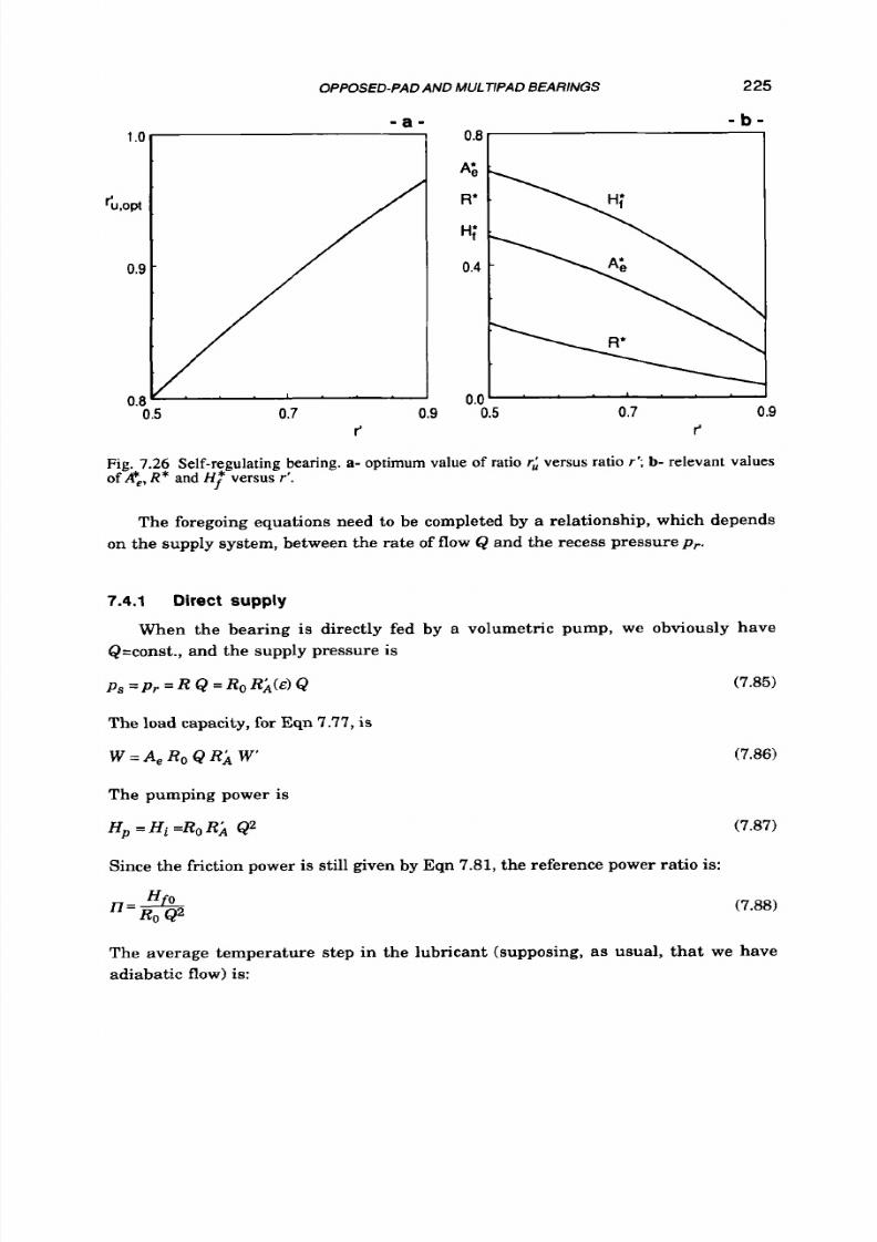
8/9/2019 Hydrostatic Lubrication 1992
http://slidepdf.com/reader/full/hydrostatic-lubrication-1992 242/558
OPPOSED-PAD AND MULTIPAD BEARINGS 225
- a -
- b -
0.0' '
.
'
0.5
0.7
0.9
f r'
Fig. 7.26 Self-regulating bearing. a- optimum value of ratio
r;
versus ratio
r'; b-
relevant values
of &e,
R* and HT
versus
r'.
The foregoing equations need to be completed by a relationship, which depends
on the supply system, between the rate of flow Q and the recess pressure
pr.
7.4.1 Direct
supply
&=const., and the supply pressure is
PS
= p r
= R
Q =RoR;1(4 Q
When the bearing is directly fed by a volumetric pump, we obviously have
(7.85)
The
oad capacity, for Eqn 7.77, is
W = A e R o Q R ; l
W '
The pumping power is
H p
=Hi
Ro R;1 Q2
Since the friction power is still given by Eqn 7.81, the reference power ratio
is:
n = H f O
Ro
Q2
(7.86)
(7.87)
(7.88)
The average temperature step in the lubricant (supposing, as usual, tha t we have
adiabatic flow) is:
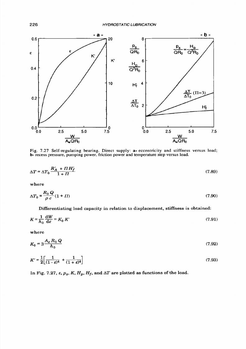
8/9/2019 Hydrostatic Lubrication 1992
http://slidepdf.com/reader/full/hydrostatic-lubrication-1992 243/558
226 HYDROSTATIC LUBRICATION
0.E
E
0.4
0.2
0.c
I
- a -
2.5 5.0
W
AeQRo
a
O
K 6
H i
0
-
T
AT0
2
- b -
1
0'
0.0
2.5 5.0 7.5
W
&Qb
Fig.
7.27 Self-regulating bearing. Direct supply: a- eccentricity and stiffness versus load;
b-
recess pressure, pumping power, friction power and temperature step versus load.
(7.89)
where
Differentiating load capacity in relation to displacemen t, stiffnes s is obtained:
where
1
K = :[ &
+ml
(7.91)
(7.92)
(7.93)
In Fig. 7.27,
E, ps,
K, H p , H f , and AT are plotted
as
functions of
the
load.
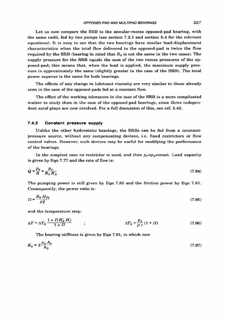
8/9/2019 Hydrostatic Lubrication 1992
http://slidepdf.com/reader/full/hydrostatic-lubrication-1992 244/558
OPPOSED-PA D AND MULTIPAD BEARINGS 227
Let us now compare the SRB
to
the annular-recess opposed-pad bearing, with
the same radii, fed by two pumps (see section
7.2.1
and section 5.4 for the relevant
equations). It is easy to see that the t w o bearings have similar load-displacement
characteristics when the total flow delivered
t o
the opposed-pad
is
twice the flow
required by the
SRB
bearing in mind that
Ro
is not the same in the two cases). The
supply pressure for the SRB equals the sum of the two recess pressures of the op-
posed-pad; this means that, when the load is applied, the maximum supply pres-
sure is approximately the same (slightly greater in the case of the SRB). The total
power expense is the same for both bearings.
The effects of any change in lubricant viscosity are very similar to those already
seen in the case of the opposed-pads fed at a constant flow.
The effect of the working tolerances in the case of the SRB is
a
more complicated
matter to study than in the case of the opposed-pad bearings, since three indepen-
dent axial plays are now involved.
For
a full discussion of this, see ref. 5.43.
7.4.2 Constant pressure supply
Unlike the other hydrostatic bearings, the SRBs can be fed from a constant-
pressure source, without any compensating devices, i.e. fixed restrictors
o r flow
control valves. However, such devices may be useful for modifying the performance
of the bearings.
In the simplest case no restrictor is used, and then p,=p,=const. Load capacity
is given by Eqn 7.77 and the rate of flow is:
(7.94)
The pumping power is still given by Eqn 7.80 and the friction power by Eqn 7.81.
Consequently, the power ratio is:
and the temperature step:
The bearing stiffness is given by Eqn 7.91, in which now
(7.95)
(7.96)
(7.97)
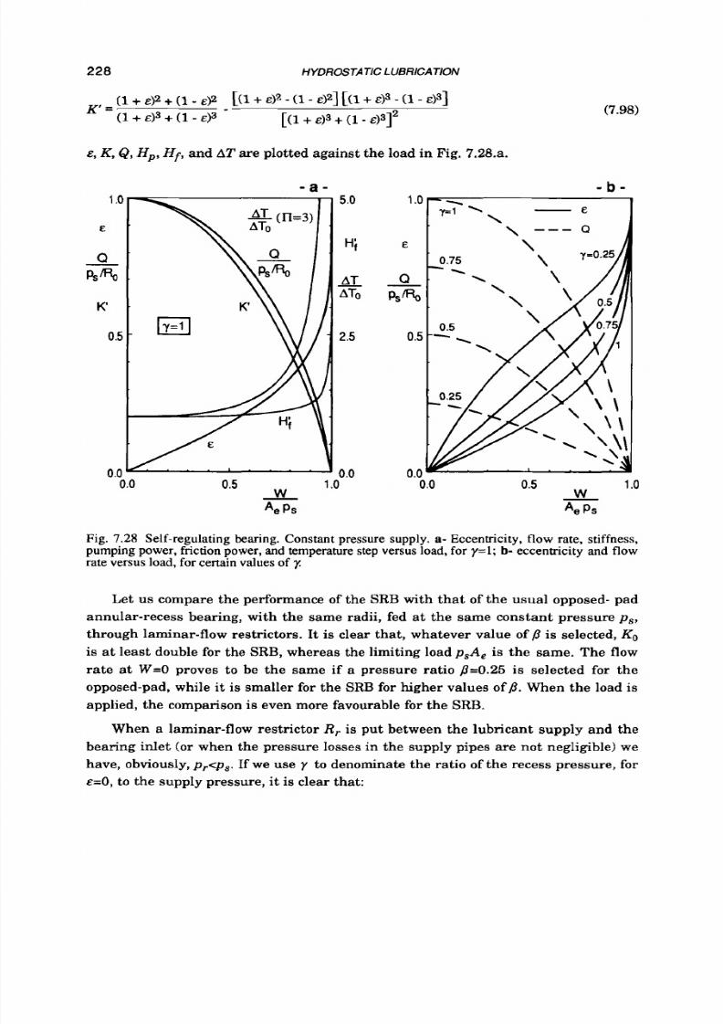
8/9/2019 Hydrostatic Lubrication 1992
http://slidepdf.com/reader/full/hydrostatic-lubrication-1992 245/558
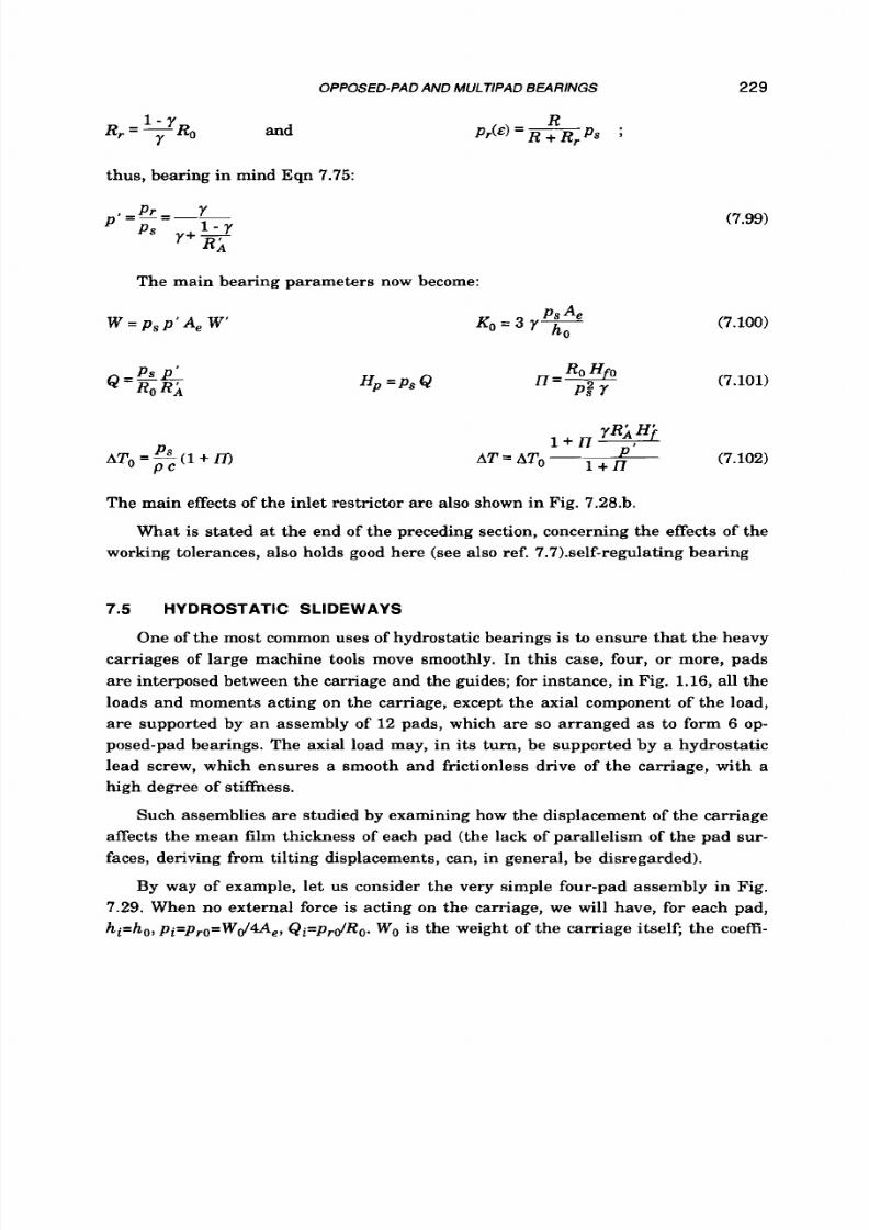
8/9/2019 Hydrostatic Lubrication 1992
http://slidepdf.com/reader/full/hydrostatic-lubrication-1992 246/558
OPPOSED-PAD AND MULTIPAD BEAR INGS
229
and
- Y
Y
R , . = - R o
thus, bearing in mind Eqn 7.75:
The main bearing parameters now become:
W = p s p ' A e W '
P
P C
AT,, = S i m
n = U
H
P? Y
(7.99)
(7.100)
(7.101)
R' H'
l + p
AT = AT^
--&+
(7.102)
The main effects of the inlet restrictor are also shown in Fig. 7.28.b.
What is stated a t the end of the preceding section, concerning the effects of the
working tolerances, also holds good here (see also ref. 7.7).self-regulating bearing
7.5
HYDROSTATIC SLIDEWAYS
One of the most common uses
of
hydrostatic bearings is to ensure tha t the heavy
carriages of large machine tools move smoothly. In th is case, four, o r more, pads
are interposed between the carriage and the guides; for instance, in Fig. 1.16, all the
loads and moments acting on the carriage, except the axial component of the load,
are supported by an assembly of 12 pads, which are so arranged as to form 6 op-
posed-pad bearings. The axial load may, in its turn, be supported by a hydrostatic
lead screw, which ensures a smooth and frictionless drive of the carriage, with a
high degree of stifiess.
Such assemblies are studied by examining how the displacement of the carriage
affects the mean film thickness of each pad (the lack of parallelism of the pad sur-
faces, deriving from tilting displacements, can, in general, be disregarded).
By way of example, let us consider the very simple four-pad assembly in Fig.
7.29. When no external force is acting on the carriage, w e will have, for each pad,
hi=ho ,p i= p r o = W d 4 Ae ,Q i= p r d Ro .W o is the weight of the carriage itselc the coeffi-
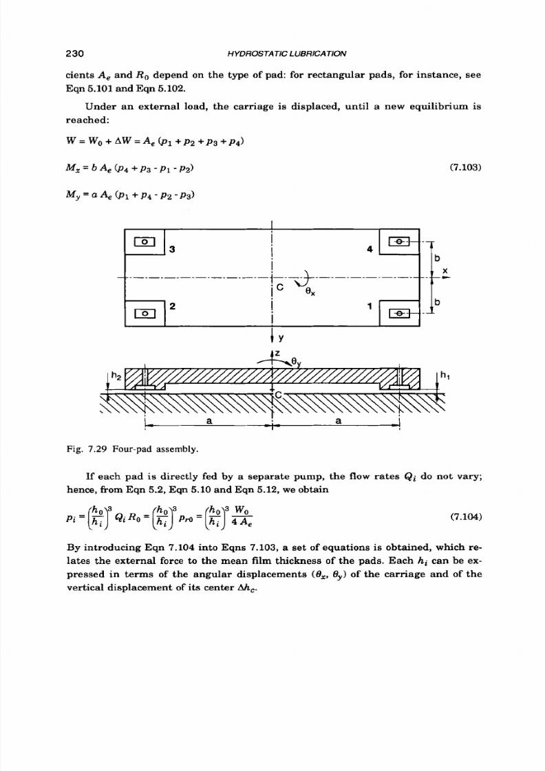
8/9/2019 Hydrostatic Lubrication 1992
http://slidepdf.com/reader/full/hydrostatic-lubrication-1992 247/558
230
HYDROSTATIC LUBRICATlON
cients A, and R o depend on the type of pad: for rectangular pads, for instance, see
Eqn 5.101 nd Eqn 5.102.
Under an external load, the carriage is displaced, until a new equilibrium
is
reached:
(7.103)
My = a Ae
(P1
+ P4 - P2 -P3)
Fig. 7.29
Four-pad
assembly.
If each pad is directly fed
by
a separate pump, the
flow
rates Qi do not vary;
hence, from Eqn 5.2,Eqn 5.10 nd Eqn 5.12,we obtain
(7.104)
By
introducing Eqn
7.104
nto Eqns
7.103,
set of equations is obtained, which re-
lates the external force to the mean film thickness of the pads. Each hi can be ex-
pressed
in
terms of the angular displacements
( O x ,
0,)
of the carriage and of the
vertical displacement of its center Ahc.
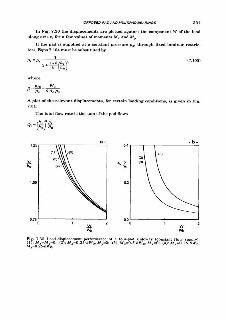
8/9/2019 Hydrostatic Lubrication 1992
http://slidepdf.com/reader/full/hydrostatic-lubrication-1992 248/558
OPPOSED-PAD AND M UiTlPA D B EAM NGS 231
In Fig. 7.30 the displacements are plotted against the component W of the load
along axis z , for a few values of moments M, nd My.
tors, Eqns 7.104must be substituted by
If the pad is supplied a t a constant pressure p s , through fixed laminar restric-
(7.105)
where
A plot of the relevant displacements, for certain loading conditions, is given in Fig.
7.31.
The total flow rate is the s u m of the pad flows
1.25
k
h0
1
oo
0.75
0
- a -
0.4
b
e x
-
ha
0.2
1
2
rc
wl
0.0
0
- b -
1 2
JY
M6
Fig.
7.30
Load-displacement performance
of
a four-pad slideway (constant flow supply).
M y = 0 . 2 5 * a d o .
(1): M,=M =O; ( 2 ) :MX=O.25 .bWo,M,=O; (3): M,=O.S.bWo, My=O; (4): M X = O . 2 5 * b W o ,
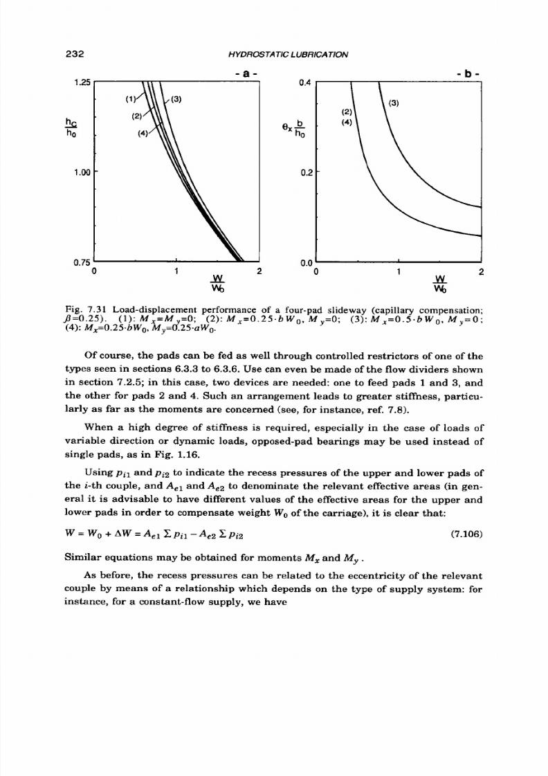
8/9/2019 Hydrostatic Lubrication 1992
http://slidepdf.com/reader/full/hydrostatic-lubrication-1992 249/558
8/9/2019 Hydrostatic Lubrication 1992
http://slidepdf.com/reader/full/hydrostatic-lubrication-1992 250/558
OPPOSED-PAD AND MULTIPAD B EARINGS
233
QiRoi
P i l = ( l - E i ) s
;
Q2
Ro2
Pi2
=
(7.107)
The eccentricities may be written as functions of the average value E=(E~+E~) /~=
and
so
on. It is then possible to evaluate the performance of
=(%+e4)/2 and
of
the angular displacements 6, and
Sy
of the carriage:
e1=E+Syu/hO-6xb/h0,
the assembly.
Greater details concerning an analytical treatment of complex pad assemblies
may be found in ref. 7.9; ref 7.10 contains results concerning a vertical boring
machine.
7.6
MULTIPAD JOURNAL BEARINGS
The multipad journal bearings may be regarded as a se t of cylindrical pads
acting on the same journal (Fig.
1.12.a).
Consequently, the load capacity of such
bearings can be evaluated, for any given displacement of the axis of the shaft from
the axis of the bearing, by calculating the load sustained by each pad, as in section
5.8, and then summing all of them together vectorial.
Although the working of the multipad bearings is simpler to understand and to
calculate (ref. 7.111, compared to multirecess ones, they are less effective and (due to
the drainage grooves separating the pads) more expensive to build. Besides, a t high
speed, the grooves may lead t o the inlet of air in the clearances.
For
these reasons,
multirecess bearings are generally preferred.
Here we shall confine ourselves to showing the load-displacement performance
of a typical four-pad bearing, fed through laminar restrictors (see Fig. 7.32). Of
course, all the other supply systems could, in principle, be used.
The reference hydraulic resistance Ro of each pad, which is necessary to design
the supply restrictors, may be calculated from Eqn 5.111 and Fig. 5.32. Hence, the
flow rate in the concentric configuration is
:
P s
Q = n P R O
(7.108)
( n is the number of pads). When the bearing is loaded, Q proves to be slightly
smaller. The pumping power and the friction power are (for E=O)
(7.109)
(7.110)
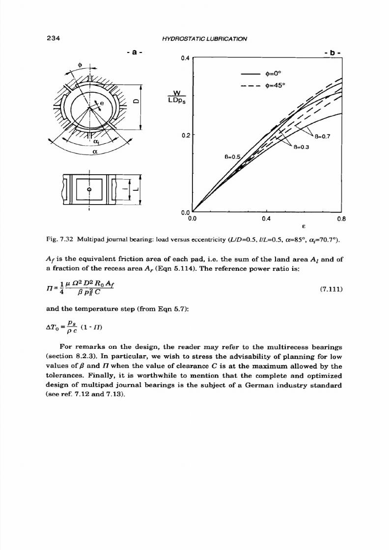
8/9/2019 Hydrostatic Lubrication 1992
http://slidepdf.com/reader/full/hydrostatic-lubrication-1992 251/558
234
- a -
HYDROSTATIC LUBRICATION
- b -
0.4
.
0.0
0.4 0.8
E
Fig.
7.32
Multipad
journal
bearing: load
versus eccentricity (LID=O.5,llL=O.5,=85",ai=70.7O).
Af is the equivalent friction area of each pad, i.e. the sum of the land area Al and of
a fraction of the recess area A,. (Eqn 5.114).The reference power ratio is:
(7.111)
and the temperature step (from Eqn 5.7):
For
remarks on the design, the reader may refer to the multirecess bearings
(section 8.2.3). n particular, we wish to stress the advisability of planning for low
values of p and
l7
when the value of clearance C s at the maximum allowed by the
tolerances. Finally,
it is
worthwhile
to
mention that the complete and optimized
design of multipad journal bearings is the subject of a German industry standard
(see ref. 7.12 and 7.13).
8/9/2019 Hydrostatic Lubrication 1992
http://slidepdf.com/reader/full/hydrostatic-lubrication-1992 252/558
OPPOSED-PAD AND MlJ lTlPA D BEARINGS
235
R E F E R E N C E S
7.1
7.2
7.3
7.4
7.6
7.6
7.7
7.8
7.9
7.10
7.11
7.12
7.13
Mueller-Gerbes
H.,
E r n s t
P.;
Maschinenelemen te z u m Um form en Drehen-
der
in
Geradlininge Bewegung;
W erkstat t und Betrieb,
11,2 (1978),65-77.
Mizumoto H., Matsubara T. , Makimoto
Y.; A
Hydrostat ical ly Control led
Restriction Sy stem for a Hydrostat ic Lead Screw;
Bull . Ja pa n
SOC.
f Preci-
sion
Eng., 0
(19861, 195-196.
Mizumoto
H.,
Okasaki
S.,
Matsubara T., Usuki M.;
An
Active Restriction
Syste m for a Hydrostatic Lead Screw; 7th Word Congr. IFToMM, Seville, 1987;
4 P.
Mizumoto H., Matsubara T., Kubo M.;
Effective Improvements
in
the Design
of Hydr ostatic Lead Sc rew;
Proc. 24th In t. MTDR Conf., 1983;p. 369-374.
Bass ani R.; Z
Pa ttini Zdrostatici Contrapposti Autoregolatori della Po rtata d i
Lubrificante;
Ingeg neria Meccanica, 24,12
(1975)) 11-18.
Bassan i R.;
The Flow Sel f -Regula t ing Hydrosta t ic Screw and N u t;
ASME
Trans. , J. Lu br. Tech., 101 (19791,364-375.
Bassani R., Piccigallo B.; The Dynamic Performance o f the Sel f -Regula ted
Hydrostatic Opposed Pad Bearing;
AGARD Conf. Proc. 323, 1982, pape r 21;
12
p.
Bassan i R., Recchia L.;
Sli t ta Zdrostat ica Alim enta ta Tr am ite Divisori di
Flusso a Spo la Conica; Ingegneria, 1979,p. 129-137.
Decker
O.,
Shapi ro
W.;
Computer-Aided Design of Hydrostat ic B earings for
Machine
Tool
Applicat ions. Part
1:
Analyt ical Foundation; Proc. 9th Int.
Decker
O.,
Sha piro W .; Computer-Aided Design of Hydrostat ic B earings for
Machine
Tool
Applications. Part
2:
Applications;
Proc. 9th Int. MTDR Conf.,
Rippel H. C.;
Hydrostatic Bearings. Part
9:
Single and Mult iple-Pad Journal
Bearings; M achine D esign, Nov. 12, 1963;p. 199-206.
Hydrostatische Radial-Gleitlager
im
Stat ionaren Betrieb (Berechnung von
Olgeschmierten Glei t lagern mit Zwischennuten);
DIN 31656, Teil 1, Nov.
1984; 29 p.
Hydrostatische Radial-Gleitlager
im
Stat ionaren Betrieb (Kenngroben f u r die
Berechnung von O lgeschmierten Glei t lagern
mit
Z w i s c h e n n u t e n ) ;
DIN
31656,Te il2 , Nov. 1984; 9 p.
MTDR Cod .,
1968;
p.
797-818.
1968;p. 819-834.

8/9/2019 Hydrostatic Lubrication 1992
http://slidepdf.com/reader/full/hydrostatic-lubrication-1992 253/558
Chapter 8
MULTIRECESS
BEARINGS
8.1
INTRODUCTION
A
multirecess journal bearing may be thought of as being derived from a multi-
pad bearing, in which the drainage grooves separating the pads disappear (Fig.
1.12.b). Even though these bearings are simpler
t o
build, more effective and there-
fore much more widely used than the multipads, they are rather more difficult
t o
calculate, since a certain amount of
flow
is now exchanged between the adjacent
recesses.
In Chapter
1 t
has already been noted tha t multirecess bearings may be classi-
fied according to the direction
of
the load that they are able
to
bear; namely, we have
axial bearings (Fig. 1.3.c), radial bearings (Fig. 1.12.b), conical and spherical bear-
ings (Fig.
1.13).A
typical application of combined radial and axial bearings, as well
as
of conical bearings,
is
in the spindles of machine tools.
8.2
ANALYSIS
The problem consists in solving the relevant Reynolds equation on the developed
land surface. For example, in the case
of
cylindrical journal bearings (Fig. 8.11, Eqn
4.18 should be used, that, in static loading conditions,
is
reduced to the following:
which may be solved by means of numerical methods, such as finite differences or
finite
element methods.

8/9/2019 Hydrostatic Lubrication 1992
http://slidepdf.com/reader/full/hydrostatic-lubrication-1992 254/558
MULTIRECESS BEA RINGS
237
Fig. 8.1
Multirecess
journal
bearing:
a- cross
section;
b-
developed surface of sleeve.
A problem now arises, since the boundary conditions are not explicitly known.
Indeed we have p=O on So andp=pi on Si, but the recess pressures
pi
depend on the
supply system and are related to the (unknown) flow ra tes Qi.
For
instance, in the
common case of compensation by means of fixed laminar-flow restrictors, we have:
A
solution can be found (ref.
B.l),
thanks
t o
the linearity of the %operator, split-
ting the differential problem
a8
follows:
Q & o ) = G p ~ C L ? s i n p(O)=O on So
;
p( 0)= 0 on
Sj
(j=l ...n)
These n + l differential problems can be solved
t o
find the pressure fields p(i)(note
that, after discretization, this may be accomplished by means of only one matrix
inversion; see, for instance, ref.
8.2).
One can now evaluate the rates of flow across
the boundaries
Si:

8/9/2019 Hydrostatic Lubrication 1992
http://slidepdf.com/reader/full/hydrostatic-lubrication-1992 255/558
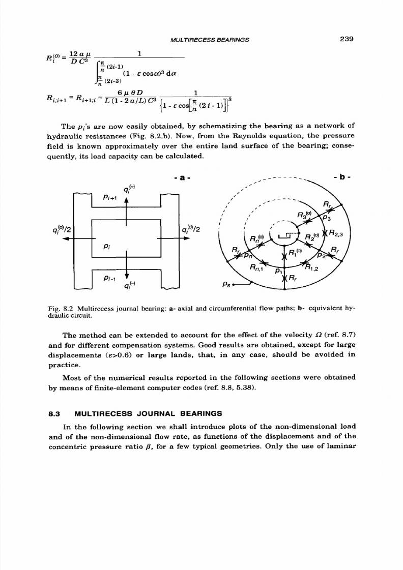
8/9/2019 Hydrostatic Lubrication 1992
http://slidepdf.com/reader/full/hydrostatic-lubrication-1992 256/558
239
The pi's are now easily obtained, by schematizing the bearing as
a
network of
hydraulic resistances (Fig. 8.2.b). Now, from the Reynolds equation, the pressure
field is known approximately over the entire land surface of the bearing; conse-
quently, i ts load capacity can be calculated.
- a -
Fig. 8.2 Multirecess journal bearing: a- axial and circumferential flow paths; b- equivalent hy-
draulic circuit.
The method can be extended to account for the effect of the velocity
R
ref. 8.7)
and for different compensation systems. Good results are obtained, except for large
displacements ( ~ > 0 . 6 ) r large lands, that, in any case, should be avoided in
practice.
Most of the numerical results reported in the following sections were obtained
by means of finite-element computer codes (ref.
8.8, 5.38).
8.3 MULTIRECESS JOURNAL BEARINGS
In the following section we shall introduce plots of the non-dimensional load
and of the non-dimensional flow rate, as functions of the displacement and of the
concentric pressure ratio /J, for a few typical geometries. Only the use of laminar

8/9/2019 Hydrostatic Lubrication 1992
http://slidepdf.com/reader/full/hydrostatic-lubrication-1992 257/558
240 HYDROSTATIC LUBRICATlON
restrictors as compensating devices will be considered in detail (plots for orifice
compensation may be found, for instance, in ref.
8.9
and for constant-flow valves in
ref.
8.10).
Parameter
p
is defined,
as
usual, as the ratio of recess pressures pi, in the
concentric configuration,
t o
the constant supply pressure
p s .
A
few approximate
expressions will also be given for load capacity, f low rate and stiffness.
The influence of the main geometrical parameters will then be explained. Fi-
nally, a number
of
remarks will be made about the design of such journal bearings.
8.3.1 Bearing performance
In Fig. 8.3, the non-dimensional load capacity
W
w'=-
P S L D
(8.3)
of a four-recess bearing is plotted as a function of eccentricity E for certain values of
ratio
L I D
and of pressure ratio p .
It
is assumed that laminar restrictors are used as
compensating devices. In the next section, we shall show how load capacity may be
affected by the varioue geometrical parameters.
In ref.
8.11
a systematic algorithm is used to obtain the load capacity, at small
0.4
W
-
LDPS
0.1
- a -
0.4
W
-
LDPS
0.2
0.L
0.0 0.4 0.8
E
- b -
0.0
0.0 0.4 0.8
E
Fig. 8.3 Multkecess
journal
bearings: load versus eccentricity, for certain values of pressure ratio3
and
of
ratio
LID ( n 4 , a'4.25, 8=30', $4').
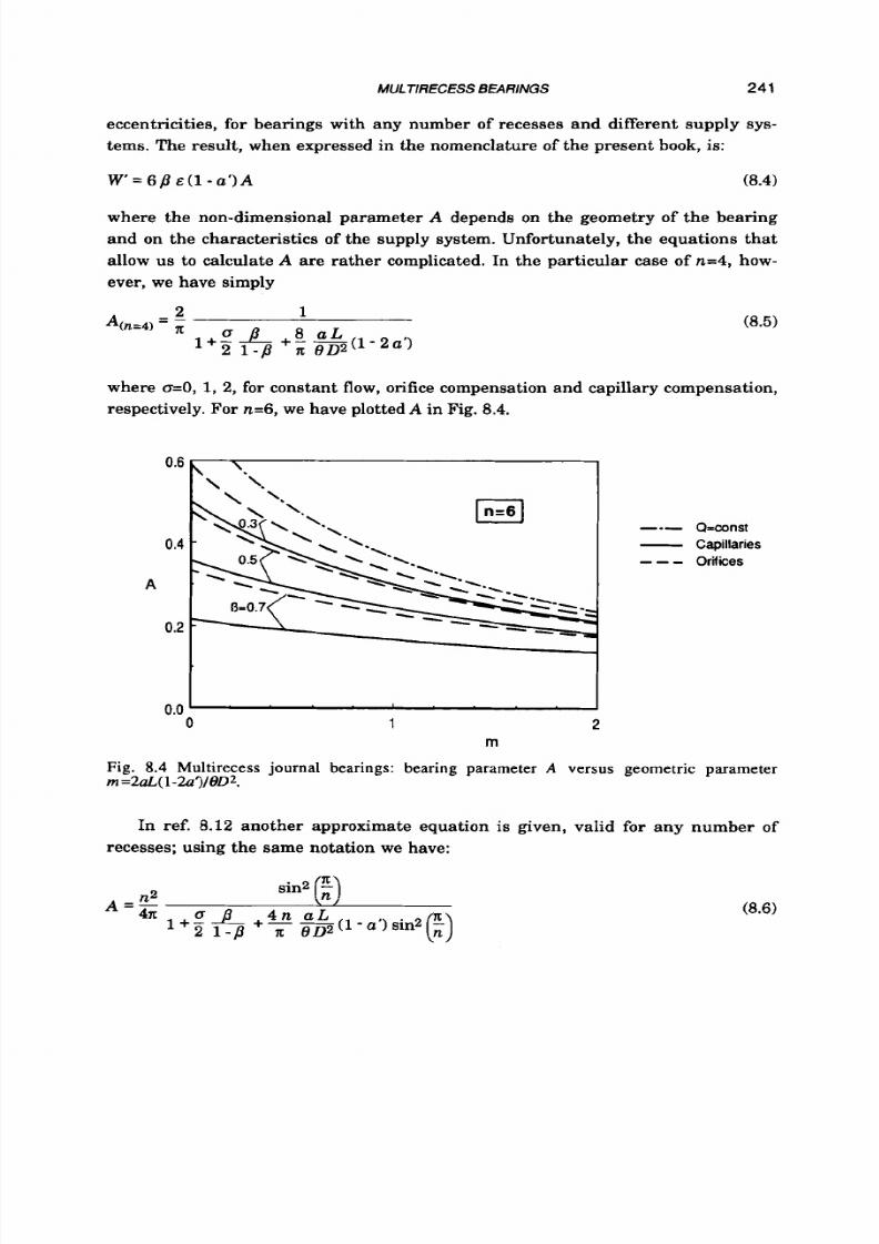
8/9/2019 Hydrostatic Lubrication 1992
http://slidepdf.com/reader/full/hydrostatic-lubrication-1992 258/558
MULTIRECESS B EARINGS 241
eccentricities, €or bearings with any number
of
recesses and different supply sys-
tems. The result, when expressed in the nomenclature of the present book, is:
W
=
6 p
~ ( 1
a ’ ) A
(8.4)
where the non-dimensional parameter A depends on the geometry
of
the bearing
and on the characteristics
of
the supply system. Unfortunately, the equations that
allow us to calculate A are rather complicated. In the particular case of n=4, how-
ever, we have simply
n 1
where
0=0,
1,2,
for
constant flow, orifice compensation and capillary compensation,
respectively. For n=6, we have plotted
A
in Fig. 8.4.
-.- a=const
- apillaries
---
Orniies
0.0
0
1
2
rn
Fig.
8.4
Multirecess journal bearings: bearing parameter A versus geometric parameter
rn=2d(1-2a’)lBD2.
In ref.
8.12
another approximate equation is given, valid for any number
of
recesses; using the same notation we have:
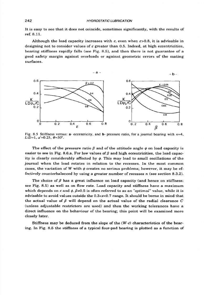
8/9/2019 Hydrostatic Lubrication 1992
http://slidepdf.com/reader/full/hydrostatic-lubrication-1992 259/558
242
HYDROSTATIC LUBRICATION
It is easy
t o
see tha t
it
does not coincide, sometimes significantly, with the results of
ref.
8.11.
Although the load capacity increases with E , even when ~ - 0 . 8 , t is advisable in
designing not t o consider values of E greater than 0.5. Indeed, at high eccentricities,
bearing stiffness rapidly falls (see Fig. 8.51, and then there is not guarantee of a
good safety margin against overloads or against geometric errors of the mating
surfaces.
- a -
- b -
0.6
0.6
0 .4 - 0.4
K K
L
D
p,/C
0.2
L D P X
0.2 -
0 I
I I
0
0 0 . 2 0.4 0.6 0.8 0 . 6 0. 8
E
Fig.
8.5
Stiffness versus:
a-
eccentricity, and b- pressure ratio, for a journal bearing with
n=4,
LID=l ,
a'=0.25,
0=30°.
The effect of the pressure ratio p and of the atti tude angle
$
on load capacity is
easier to see in Fig. 8.6.a. For low values of and high eccentricities, the load capac-
ity is clearly considerably affected by $. This may lead to small oscillations of the
journal when the load rotates in relation to the recesses. In the most common
cases, the variation of W with
$
creates no serious problems; however, i t may be ef-
fectively counterbalanced by using a greater number of recesses
n
(see section
8.3.2).
The choice of
p
has a great influence on load capacity (and hence on stiffness:
see Fig.
8.5)
as well as on flow rate. Load capacity and stiffness have a maximum
which depends on E and $.
/3=0.5
is often referred
t o
as an "optimal"value, while it is
advisable to avoid values outside the
0.3c~c0.7
ange. It should be borne in mind that
the actual value of will depend on the actual value of the radial clearance C
(unless adjustable restrictors are used) and then the working tolerances have a
direct influence on the behaviour of the bearing; this point will be examined more
closely later.
Stiffness may be deduced from the slope
of
the ( W - E ) haracteristics of the bear-
ing. In Fig. 8.5 the stiffness of a typical four-pad bearing is plotted as a function of
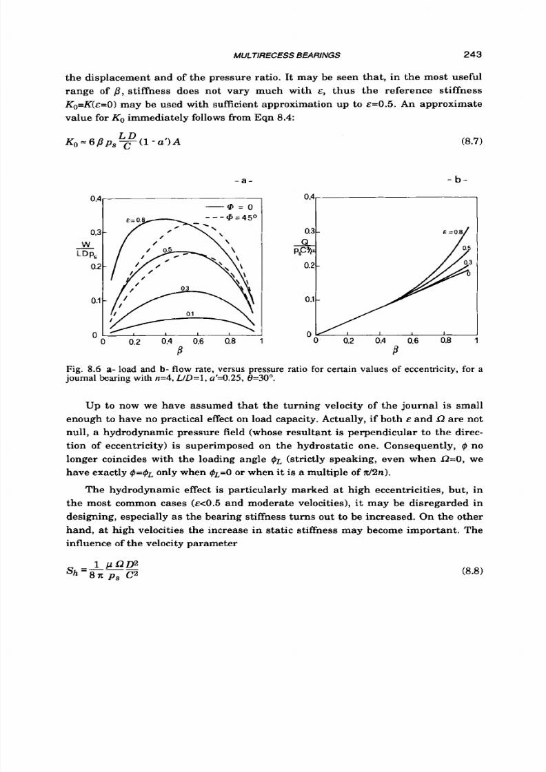
8/9/2019 Hydrostatic Lubrication 1992
http://slidepdf.com/reader/full/hydrostatic-lubrication-1992 260/558
MULTIRECESS
BEARINGS 243
the displacement and of the pressure ratio. It may be seen that, in the most useful
range of 8 , stiffness does not vary much with E , thus the reference stiffness
Ko=K(&=O) ay be used with sufficient approximation up to ~ = 0 . 5 . n approximate
value for
KO
mmediately follows from Eqn 8.4:
(8.7)
D
KO
6 B p ,7 1
u ' ) A
- a -
0.4
-9 =
0
' I / / - \ \
Fig. 8.6 a- load and b- flow rate, versus pressure ratio for certain
values
of eccentricity,
for a
journal bearing with n=4, L / D = l , ~ ' 4 . 2 5 ,=30°.
Up to now we have assumed that the turning velocity of the journal
is
small
enough to have no practical effect on load capacity. Actually, if both E and R are not
null, a hydrodynamic pressure field (whose resultant is perpendicular t o the direc-
tion of eccentricity) is superimposed on the hydrostatic one. Consequently, 4 no
longer coincides with the loading angle
+L
(strictly speaking, even when R=O, we
have exactly +=$L only when
+L=O
or when it
is
a multiple of
d2n).
The hydrodynamic effect is particularly marked at high eccentricities, but, in
the most common cases ( ~ < 0 . 5 nd moderate velocities),
it
may be disregarded in
designing, especially as the bearing stiffness turns out to be increased. On the other
hand, at high velocities the increase in static stiffness may become important . The
influence of the velocity parameter

8/9/2019 Hydrostatic Lubrication 1992
http://slidepdf.com/reader/full/hydrostatic-lubrication-1992 261/558
244 HYDROSTATIC LUBRICATION
- a -
2.0
W '
-
0.0
0.2
0.4 0.0 0.2 0.4
Sh Sh
Fig. 8.7 a- load and b- attitude angle, versus speed parameter S (Sommerfeld hybrid number)
for
two
journal bearings with different ratio LID and
n=4, a'd.25, b=3Oo, #=Oo,J?=0.5.
(often called the
"Somm erfeld hybrid number")
on
W
and on the angle
#L-#,
s
shown in Fig.
8.7
for a few typical cases.
Hydrodynamic load capacity is calculated in ref. 8.11 as
Total load capacity is the vectorial sum of the hydrostatic and hydrodynamic terms;
therefore, a "speed enhancement factor" may be calculated:
(8.10)
which is not dependent on the number of recesses. For small values of E, the actual
load capacity may be approximately evaluated by multiplying W(a=O) y the same
factor K , . Other workers suggest different equations. For instance, in ref. 8.12
similar results have been obtained, except for (1 2 a ' ) in Eqn 8.9 and Eqn 8.10 is
substituted with (1 a').
In consequence
of
the above, it seems profitable to design in such a way
as
to
have high values of S h , in order t o take advantage of the great increase in load ca-
pacity. However, it must be stressed that the increase in the speed parameter cre-
ates certain undesirable consequences. In particular, in certain recesses, the pres-
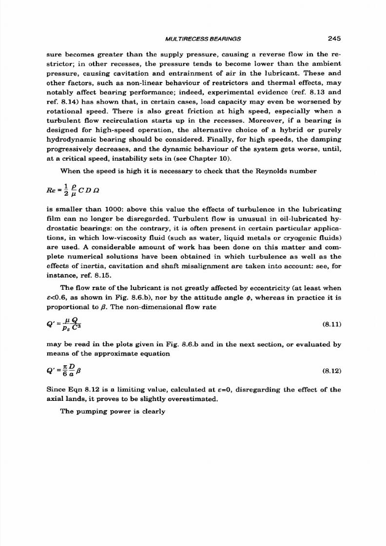
8/9/2019 Hydrostatic Lubrication 1992
http://slidepdf.com/reader/full/hydrostatic-lubrication-1992 262/558
MULTIRECESS
BEARINGS
245
sure becomes greater than the supply pressure, causing a reverse flow in the re-
strictor; in other recesses, the pressure tends t o become lower than the ambient
pressure, causing cavitation and entrainment of air in the lubricant. These and
other factors, such as non-linear behaviour of restrictors and thermal effects, may
notably affect bearing performance; indeed, experimental evidence (ref.
8.13
and
ref.
8.14)
has shown that, in certain cases, load capacity may even be worsened by
rotational speed. There is also great friction a t high speed, especially when
a
turbulent flow recirculation star ts up in the recesses. Moreover, if a bearing is
designed for high-speed operation, the alternative choice of a hybrid o r purely
hydrodynamic bearing should be considered. Finally, for high speeds, the damping
progressively decreases, and the dynamic behaviour of the system gets worse, until,
a t a critical speed, instability sets in (see Chapter 10).
When the speed is high i t is necessary
t o
check that the Reynolds number
1 P
R e = - - C D R
2 P
is smaller than
1000:
above this value the effects of turbulence in the lubricating
film can no longer be disregarded. Turbulent flow is unusual in oil-lubricated hy-
drostatic bearings: on the contrary, it is often present in certain particular applica-
tions, in which low-viscosity fluid (such as water, liquid metals o r cryogenic fluids)
are used. A considerable amount of work has been done on this matter and com-
plete numerical solutions have been obtained in which turbulence a s well as the
effects of inertia, cavitation and shaft misalignment are taken into account: see, for
instance, ref. 8.15.
The flow rate
of
the lubricant is not greatly affected by eccentricity (at least when
&<0.6,as
shown in
Fig. 8.6.b),
nor by the attitude angle
9 ,
whereas in practice it is
proportional to
p.
The non-dimensional flow rate
-&§
Q ' - p s
c3
may be read in the plots given in Fig.
means of the approximate equation
(8.11)
8.6.b and
in
the next section, or evaluated by
(8.12)
Since Eqn 8.12 is a limiting value, calculated a t &=O, disregarding the effect of the
axial lands,
it
proves to be slightly overestimated.
The pumping power is clearly
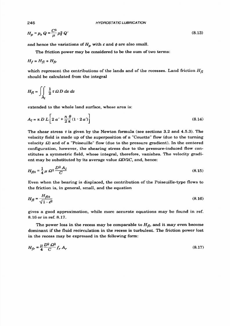
8/9/2019 Hydrostatic Lubrication 1992
http://slidepdf.com/reader/full/hydrostatic-lubrication-1992 263/558
246
HYDRWTA
T1C
LUBRlCATlON
(8.13)
and hence the variations of
H p with E
and I$ are also small.
The friction power may be considered to be the
s u m
of two terms:
which represent the contributions of the lands and
of
the recesses. Land friction Hfi
should be calculated from the integral
extended to the whole land surface, whose area is:
(8.14)
The shear stress
z
is given by the Newton formula (see sections 3.2 and 4.5.3). The
velocity field is made up of the superposition of a "Couette" flow (due to the turning
velocity 52) and of a "Poiseuille" flow (due to the pressure gradient). In the centered
configuration, however, the shearing stress due t o the pressure-induced flow con-
stitutes a symmetric field, whose integral, therefore, vanishes. The velocity gradi-
ent may be substituted by its average value LlDJ2C, and, hence:
(8.15)
Even when the bearing is displaced, the contribution of the Poiseuille-type flows
t o
the friction is, in general, small, and the equation
(8.16)
gives a good approximation, while more accurate equations may be found in ref.
8.16
o r in ref.
8.17.
The power loss in the recess may be comparable to H f l , and
it
may even become
dominant if the fluid recirculation in the recess is turbulent. The friction power lost
in the recess may be expressed in the following form:
(8.17)

8/9/2019 Hydrostatic Lubrication 1992
http://slidepdf.com/reader/full/hydrostatic-lubrication-1992 264/558
MULTIRECESS BEARINGS
where A,.
is
the total recess area:
A,. =
R
D
L
(1 - 2a') 1 -%
(
" 7
247
(8.18)
The coefficient
f,
depends on the ratio
Clh,
and on the Reynolds number
(8.19)
P
Re, = -- D 52 h,
2P
If we have Rer<lOOO (laminar flow)and C<<h,, i t may simply be taken that fr=4Clh,,
or better (ref.
4.5):
(8.20)
In the case of turbulent flow, f, may be calculated from Eqn 4.54.
Lastly, the friction moment and the friction power may be written as follows:
(8.21)
D2
M f = p R
c
f
H f = R M f (8.22)
where the equivalent friction area
A f
may be calculated from the following equation:
(8.23)
Plots of A; are given in Fig. 8.8.
A t
the highest speeds the torque required t o accelerate the fluid entering the
bearing (momentum torque)may become notable. It may be calculated (ref. 8.19) as:
(8.24)Q
= ; I P Q
c Re
D
where the Reynolds number is
1 P
R e = - - C D R
2 P
The relevant power loss
is
obviously
H Q = N Q .
It is interesting to compare H Q with the pumping power:
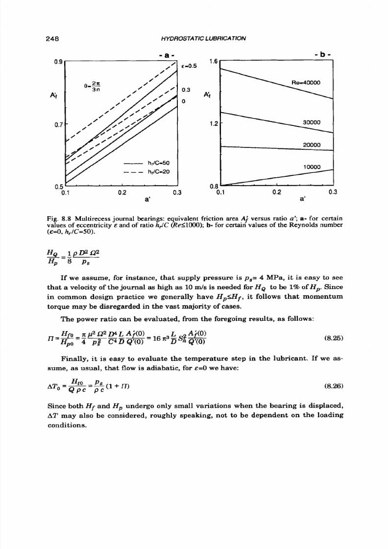
8/9/2019 Hydrostatic Lubrication 1992
http://slidepdf.com/reader/full/hydrostatic-lubrication-1992 265/558
248
HYDROSTATIC LUBRICATION
- a -
E-0.5
0.3
0
0.5'
' ' ' ' '
.
. '
. '
0.1
0.2
0.3
a'
- b -
20000
0000
0.8
0.1 0.2 0.3
a'
Fig. 8.8 Multirecess
values of eccentricity
(~4,, ./C=50).
journal bearings: equivalent friction area
A?
versus ratio
a'; a-
for certain
'
E and of ratio h,JC
(ReS1000);
b- or certain values of the Reynolds number
If we assume, for instance, that supply pressure
is ps= 4
MPa,
it
is easy to see
that
a
velocity of the journal
as
high as 10m/s
is
needed for H g to be 1%
of Hp.
Since
in common design practice we generally have Hpmf,t follows that momentum
torque may be disregarded in the vast majority of cases.
The power ratio can be evaluated, from the foregoing results, as follows:
(8.25)
Finally, it is easy to evaluate the temperature step in the lubricant. If we as-
sume, as usual, that flow is adiabatic, for E=O we have:
(8.26)
Since both
Hf
nd
H p
undergo only small variations when the bearing
is
displaced,
AT may also be considered, roughly speaking, not to be dependent on the loading
conditions.

8/9/2019 Hydrostatic Lubrication 1992
http://slidepdf.com/reader/full/hydrostatic-lubrication-1992 266/558
MULTIRECESSBEARINGS
249
8.3.2 Effect of geometr ical parameters
The geometrical ratios which may affect both load capacity and flow rate are
LID, a ' = a l L , 8 (see Fig. 8.1). Besides, the number of the recesses should also be
considered.
The value of
n
could, in theory, be anything, provided
it
is greater than
3,
but
values greater than 6 are seldom encountered; indeed, the benefit of further in-
creasing
n
diminishes and hardly counterbalances the greater manufacturing
costs and the greater complexity of the supply system.
In brief, the main consequences of increasing the number of recesses are that
load capacity and stiffness are higher and, moreover, are less dependent on the atti-
tude angle
$.
The rate of flow a t any given eccentricity is practically unaffected. The
load capacity of a 6-recess bearing is plotted in Fig.
8.9,
which should be compared
with the analogous Fig. 8.6.
- a -
- b -
I
I
I
4
3.2
Q21A
P,C P
1.6
0.8
0
0 Q 2 0.4
0.6
0.8 1 0 0.2
0.4
0.6 0.8 1
B B
Fig. 8.9
a-
load and
b-
flow rate, versus pressure ratio for certain values
of
eccentricity,
for
a
journal bearing with
n=6, L / D = l , ~ ' 4 . 2 5 ,=30°.
The effect of
a l L
and
L I D
is shown in Fig.
8.10.
To increase the parameter
a l l
means to increase the land area to the detriment of the recess area; consequently,
the load capacity decreases with a quasi-linear trend. On the other hand, the flow-
rate is approximately proportional t o
L
1a; ince the pumping power is proportional
to Q ' I W'2 (once load W, eccentricity
E ,
and the other geometrical parameters are
fixed), a value of a' clearly exists a t which the required pumping power is a mini-
mum. This occurs, roughly speaking, when a'=0.3; however, this value is not criti-
cal and, in general, it proves t o be advisable to design a larger recess to step up load
capacity and reduce friction, which, indeed, mainly depends on the developed land

8/9/2019 Hydrostatic Lubrication 1992
http://slidepdf.com/reader/full/hydrostatic-lubrication-1992 267/558
250
HYDROSTATIC LUBRICATION
- a - - b -
0.0
I
"
0.1
0.2
0.3 0.1
0.2 0.3
a' a'
Fig.
8.10
Multirecess journal bearings:
a-
load and
b- f l ow
rate, versus
a', for
certain values of
ratio LID ( n 4 , =30 , = 4 5 O , J = O . 4 ) .
area Al. Most authors propose "optimal" values for a' in the 0.2510.1 range, o r even
smaller (see ref. 8.17
for
a review); some maintain that a recess area
A,.=O.hDL
is
a
good compromise between high load capacity and low power loss (see ref. 8.20).
Actually, a more detailed analysis (ref. 8.21) would show tha t even a t moderate
speeds (n<l)t is convenient
to
select small values of a' (a'=0.1) n order to reduce H t
and
AT.
At higher speeds, since the hydrodynamic effect becomes appreciable,
slightly greater values of a' may be convenient from the point of view of power loss
(but not from the point of view of temperature). Indeed, in ref. 8.23, it is suggested
that a'=0.15 be selected (independently from the number of recesses and from the
LID
ratio)
for
a
power ratio
n=2;
his
is
no doubt a good choice for the entire most
usual range of power ratios, that is
n=l-t3.
inally, a t very high speeds n>3),he
power loss
is
the smallest for vanishing recesses: this explains the peculiar design
of
hybrid
bearings (see chapter
9).
Concerning LID, since W' decreases as LID grows,
it
is clearly more convenient
to increase D instead of L in order to enlarge the projected area and hence increase
load capacity. On the other hand, flow rate and pumping power are approximately
proportional to D JL,and do not depend on the projected area. Furthermore, Giction
power is proportional to D4L (Eqn
8.22) .
Thus, to reduce power loss, it seem advis-
able to have high L
1D
ratios. L /D=1 s often proposed as a good compromise.

8/9/2019 Hydrostatic Lubrication 1992
http://slidepdf.com/reader/full/hydrostatic-lubrication-1992 268/558
MULTIRECESS B EARINGS 251
The effect of the land angle 8 is shown in Fig. 8.11.
A s
can be seen, the flow-rate
does not vary s o much with 0, whereas the load capacity improves, increasing
8,
o
a certain extent, which depends on
E,
4, a' and
p.
This is not surprising, because the
separation of the recesses is improved even though the recess area is reduced.
However, values of 8 greater than 2 d 3 n (i.e. 30 degrees for n = 4 ) provide no great
benefit, while friction power always grows with 8. Also
H ,
and
AT
are influenced by
the recess angle 8. n ref. 8.21 it
is
shown that the temperature step decreases when
8 s increased up to a certain value, which depends on ll and a', and then remains
practically constant. For instance, for L I D = l , n = 4 , 8 = 0 . 5 , a '= 0 .1 and I7=1, 8 should
not be smaller than 18". Greater values may be suggested for higher values of I7 and
a'. From the point of view of total power an optimal value
of 8
may be determined:
for n=4 and moderate speed, this vanes in the 18"+30"range, when
a'
is between
0.1
and 0 . 2 . In ref. 8.23 i t
is
suggested that8
=0.5
rad be selected
for
n=4 and L I D = l and
smaller values when n is greater and L I D is smaller (e.g. 8 =0.5 for n = 1 2 and
L I D 4 . 3 ) .
0.4
W
-
LDP,
0.2
0.0
- a -
a'=0.1
@
- b -
0.2
0.25
"
10" 20 30"
40
10" 20" 30" 40
Fig. 8.1
1
Multirecess journal bearings: a- load and
b-
concentric
flow
rate, versus land angle
8,
for certain values of ratio a'; ( n 4 , /D=l,J=O.4).
8.3.3
Design of mul t i recess journa l bear ings
Design criteria for journal bearings are not so different from those proposed in
section
7 . 2 . 6 ,
concerning opposed-pad bearings. As usual i t will be assumed that the
main objective consists in obtaining a certain load capacity
W,
with a smaller dis-
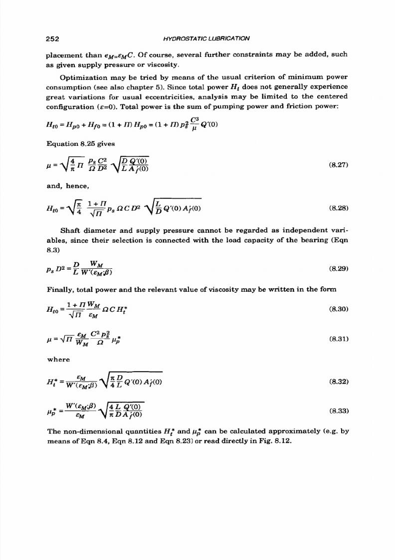
8/9/2019 Hydrostatic Lubrication 1992
http://slidepdf.com/reader/full/hydrostatic-lubrication-1992 269/558
252 HYDROSTATIC LUBRlCATlON
placement than
eM=EMC.
Of course, several further constraints may be added, such
as given supply pressure o r viscosity.
Optimization may be tried by means of the usual criterion of minimum power
consumption (see also chapter 5). Since total power
H ,
does not generally experience
great variations for usual eccentricities, analysis may be limited to the centered
configuration ( E=O) .
Total
power is the sum of pumping power and friction power:
Equation 8.25 gives
and, hence,
(8.27)
(8.28)
Shaft diameter and supply pressure cannot be regarded
as
independent vari-
ables, since their selection is connected with the load capacity of the bearing (Eqn
8.3)
D W M
P s D2 =L W'(EM;rO)
(8.29)
Finally, total power and the relevant value of viscosity may be written in the form
where
(8.30)
(8.31)
(8.32)
(8.33)
The non-dimensional quantities
H:
and
1
can be calculated approximately (e.g. by
means of Eqn 8.4, Eqn 8.12 and Eqn 8.23)or read directly in Fig. 8.12.

8/9/2019 Hydrostatic Lubrication 1992
http://slidepdf.com/reader/full/hydrostatic-lubrication-1992 270/558
MULTIRECESS
BEARINGS
253
Examining Eqn 8.30, one may easily draw the same conclusions as those
reached in the case of Eqn 6.57 o r Eqn 7.64, concerning thrust bearings.
For
given
values of clearance and speed, the "op t imal" value of viscosity is the one which
ensures
a
power ratio
n=1.
However this value is not critical, since
H t
experiences
only small variations for values of the power ratio in the range 1/3t3.
Concerning clearance, i t is clearly convenient to reduce i t a s far a s possible, in
order
t o
obtain small power and high stiffness. Limits to the selection of very small
clearances follow from two types of considerations. Firstly, Eqn 8.31 shows that a
very small clearance may require an impracticably low viscosity to obtain n=1, ven
after a small land width has been selected, in order t o reduce pp*. In certain cases
the value of viscosity is a design constraint, and i t may be shown that when p is
given, the lowest value of
Hto
is obtained by selecting
C
n such a way as
to
have
n=3.
I
0.1
0.2 0.3
a'
- b -
1.5
- =0.5
- - - €10.3
0.0'
. I . . . .
0.1
0.2 0.3
a'
Fig. 8.12 Multirecess journal bearings: a- total power H : and b- relevant viscosity p; versus
ratio a'
for
certain values of ratio LID and of working eccentricity E; (n=4, 8=3# ,$=45 ,J=#.4,
f,=#.2)
Another limit
to
the selection of C is connected with manufacturing tolerances
(ref. 8.241. Indeed, the designer must often select a whole range CmlCIC, instead
of a single value and, if the tolerance 6g=2(CM-Cm)
s
large, the actual performance
of the bearing may differ notably from the one calculated. Let us assume that the
maximum radial clearance CM.has been selected in such
a
way as to satisfy all the
design constraints with a certain value B of the concentric pressure ratio. When

8/9/2019 Hydrostatic Lubrication 1992
http://slidepdf.com/reader/full/hydrostatic-lubrication-1992 271/558
254
HYDROSTATIC
LUBRICATION
E=O, the flow rate is proportional to
C-3:
it is now clear tha t the actual pressure ratio
will be
1
f i l l =
1-p
c
3
l +
P
(G)
(8.34)
Since it is convenient to impose an upper limit /lM on the pressure ratio, to avoid a
sharp decrease in load capacity (see Fig. 8.6.a)) we readily obtain
(8.35)
For example, if
p=0.4
and
8 ~ = 0 . 7 ,
e must have
c , / c~>0 .66 ,
.e.
6g<2/3'cMM.
on-
sequently,
CM
cannot be too small, otherwise an excessively small tolerance would
be required. The actual value of the power ratio also depends on the actual value of
clearance. Namely, if n s the designed power ratio tallying with the greatest clear-
ance C for any other clearance
w e
get
which, strictly speaking, is not valid when recess friction makes a predominant
contribution to the total power loss (e.g. in the case of turbulent flow in the recess).
I t is worth noting that if
p=0.4, n=1
and
c,=2/3'cM,
the greatest relevant value of
the concentric power ratio proves
to
be close to
3.
We wish to stress that the foregoing considerations concerning the optimal
design of such bearings are based on a simplified analysis, which nevertheless
gives good results. In particular, the increase in load capacity due to the hydrody-
namic effect has not been taken into account, and total power has been evaluated for
E=O instead of a t a working eccentricity. It is also worth noting that there is a turbu-
lent recess flow in the case of high-speed bearings. Consequently, coefficient
f,
s
much greater than the value assumed in Fig.
8.12
and, above all, H t and p; cannot
be considered t o be virtually independent from p,D and
C .
Several authors express
different points of view, obtaining somewhat different results (see, for example, ref.
8.17
and
8.18
for a review). In particular, i t must be remembered that the optimized
design of multirecess journal bearings is the subject of a German industrial stan-
dard (ref.
8.22
and
8.23).
Direct optimization methods have also been proposed,
based on well-known optimization algorithms such as the
complex method
or the
f lexible polyhedron method, in which the object function (e.g. the
H ,
J W ratio) is
found by solving the Reynolds equation by means of finite-difference or finite-
element methods (ref. 8.25).
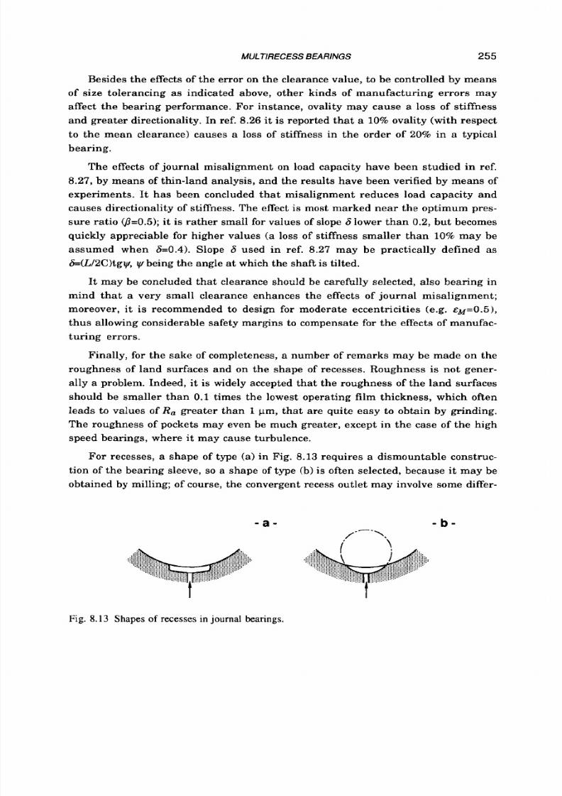
8/9/2019 Hydrostatic Lubrication 1992
http://slidepdf.com/reader/full/hydrostatic-lubrication-1992 272/558
MULTIRECESS BEARINGS 255
Besides the effects
of
the error on the clearance value, to be controlled by means
of
size tolerancing
as
indicated above, other kinds of manufacturing errors may
affect the bearing performance. For instance, ovality may cause a loss of stiffness
and greater directionality. In ref. 8.26
it
is reported tha t a 10% ovality (with respect
to the mean clearance) causes a loss of stiffness in the order of 20% in a typical
bearing.
The effects of journal misalignment on load capacity have been studied in ref.
8.27, by means of thin-land analysis, and the results have been verified by means of
experiments. It has been concluded that misalignment reduces load capacity and
causes directionality
of
stiffness. The effect
is
most marked near the optimum pres-
sure ratio
@=0.5);
t is rather small for values of slope
6
lower than 0.2, but becomes
quickly appreciable for higher values (a loss of stiffness smaller than 10% may be
assumed when
6=0.4).
Slope 6 used in ref. 8.27 may be practically defined as
6=(L/2C)tg~,
y
being the angle a t which the shaft is tilted.
It
may be concluded that clearance should be carefully selected, also bearing in
mind that a very small clearance enhances the effects of journal misalignment;
moreover, it is recommended to design for moderate eccentricities (e.g.
~ ~ = 0 . 5 ) ,
thus allowing considerable safety margins
t o
compensate for the effects of manufac-
turing errors.
Finally, for the sake
of
completeness, a number
of
remarks may be made on the
roughness
of
land surfaces and on the shape of recesses. Roughness is not gener-
ally a problem. Indeed,
it
is widely accepted that the roughness of the land surfaces
should be smaller than 0.1 times the lowest operating film thickness, which often
leads to values of R , greater than
1
pm, that are quite easy to obtain by grinding.
The roughness of pockets may even be much greater, except in the case of the high
speed bearings, where it may cause turbulence.
For recesses, a shape of type (a) in Fig. 8.13 requires a dismountable construc-
tion of the bearing sleeve,
so
a
shape
of
type (b)
is
often selected, because it may be
obtained by milling; of course, the convergent recess outlet may involve some differ-
- a - - b -
/----\.
i
\
Fig. 8.13
Shapes
of
recesses
in
journal bearings.

8/9/2019 Hydrostatic Lubrication 1992
http://slidepdf.com/reader/full/hydrostatic-lubrication-1992 273/558
256 HYDROSTATIC LUBRICATION
ences in the behaviour of the bearing. Particular recesses have also been proposed
in order to reduce recess friction in high-speed bearings (ref. 8.28).
8.3.4
Design procedure
Following the remarks made above, a simple procedure may be proposed, that
should lead to an "optimized"design of opposed-pad bearings. As before
it
will be
assumed that a certain load W M is given, to be sustained with a displacement
smaller than eM at a speed iz; some further constraints may be required: the design
may then be carried out following the steps below.
i) Choose a trial set of geometric parameters; perhaps
L I D = l ,
alL=0.15,
0=30°,
n=4;
it is convenient to select large recesses (i.e. small values of
a )
unless
low speeds are expected.
Choose a trial value of the maximum eccentricity, such as ~~=0.5.
Take
p=0.4
as the design pressure ratio: a smaller value can be accepted if
n>4or
&&0.5.
ii ) Evaluate coefficient
W'
by means of figures given in the preceding sections.
Select a suitable supply pressure
p s ,
if it is not given.
Calculate a first value for diameter D , by means of Eqn 8.29.
Check the temperature step (Eqn 8.26); since for many mineral oils we have
~ ~ - 1 . 6 . 1 0 ~/m3"C, and i t should be
n < 3 ,
the maximum temperature step is
expected
t o
be AT<pS.2.5"CIMPa.
iii) Select a suitable value for the manufacturing tolerance Sg=2(C~-Cm):ee
also Fig. 8.14; bear in mind that the narrower Sg is, the lower the power
losses can be.
Take Crn+ and cMM=cm+6g/2.
Check if stiffness is great enough. Otherwise reduce
Sg
or select a smaller
value for EM, restarting from point
(ii).
iv) Calculate the "optimal"value of viscosity, i.e. the value k p t that leads
to n=1
when C=C, (Eqn 8.31).
Check that
kpt
s a plausible value (sometimes p may be directly imposed by
the specifications); if it is not, try
t o
modify the geometrical parameters
(namely the recess width), the clearance or the supply pressure. However, if
R is very low it will not be possible
to
get
n=1
indeed, for 8=0, n "infinite"
viscosity would be required ); in this case select the highest allowable viscos-
ity, and
a
larger land width, such
as
a'=0.25, On the contrary,
a
very
high
speed would lead to values too small for
h p t ;
in this case
it
will be necessary
to accept values of the maximum power
ratio
(tallying with the least clear-
ance
C , )
greater than 3 : the ensuing hydrodynamic effect will enhance

8/9/2019 Hydrostatic Lubrication 1992
http://slidepdf.com/reader/full/hydrostatic-lubrication-1992 274/558
MULTIRECESS B EARINGS
i o o l
IT=7
"1
0 18
30 50
80
120 180
250
D [mml
257
Fig.
8.14
Values of parameter
6g=2(C,+,-C,),
for certain international tolerance (IT) grades
(ISOIR286).
bearing stiffness, but any of the problems already noted might arise
(cavitation, excessive warming of lubricant, and even dynamic instability).
v) Calculate flow rate, pumping power, friction torque and friction power, with
reference to the design configuration (C=CM, =O) .
Check the same parameters for different values of
C
and
E.
If
flow
rate seems too great, and
6
cannot be further reduced, it will be
necessary to accept a power ratio
n>l
(e.g. increasing p or reducing
p s )
consequently increasing friction. Conversely, friction may be easily reduced
with a larger expense of flow rate and pumping power.
I f the supply system is not able
t o
maintain lubricant viscosity within a
narrow range, check friction and the temperature step for the maximum
expected viscosity, and check the flow rate for the minimum viscosity.
vi)
Design the compensating restrictors.
vii) Check the Reynolds number in the bearing clearances and in the recess.
viii)
Check the dynamic behaviour of the system (see Chapter 10).
EXAMPLE 8.1
Design a m ultirecess bearing to sustain a journal, w hose diam eter is D =80 m m,
rotating at a speed i2110.5
r a d l s
(-1000
pm); the operating load W l tO
KN
must be
susta ined wi th a d isplacement smaller than e ~ = 2 0m; manufacturing tolerances

8/9/2019 Hydrostatic Lubrication 1992
http://slidepdf.com/reader/full/hydrostatic-lubrication-1992 275/558
258 HYDROSTATIC LUBRICATION
should not be smaller t ha n IT5 grade for both journ al an d s leeve; supply pressure
m ay not be greater tha n 5 MPa.
i ) Let us select a trial set of para me ters: L I D = l , a'=0.15, n=4, 9=30°, ~ ~ = 0 . 5 ,
8=0.4.
i i) F r om F ig , 8 .1 1 w e m a y read W ( ~ ~ ) = 0 . 2 6 9 ;t is clear (E qn 8.29) that , d ue to the
cons tra in ts on pressure and shaf t d iameter , the m ax im um operat ing load cannot
be sustained w it h a n eccentricity ~ ~ = 0 . 5actually it sh ou ld be W p 8 . 6 KN) . I n order
to increase load capacity, one ma y try to increase the a xial len gth o f the s leeve and
to reduce the width of the circumferential lands (to increase the number of recesses
would also have a notable effect on load capacity). Selecting LID=1.25 and a'=O.1, a
sim ple interpolation of available da ta gives W'(&=0.274, and hence wM=ll.o
kW
wi th a supply pressure ps=5 MPa.
i i i) Since the tolerance grade is given, the w idt h of th e tolerance range for di -
ametral clearance must be Gg=2(C~-C,,J=26m; hence, a suitable choice for radial
c learance m ay be C=40+27 pm. Note tha t , assuming h o = C ~ = 4 0 m as the reference
c lear ance , a t the eccen t r i c i t y EM =0.5 w e h a v e a n a c t u a l d i s p la c e m e n t
e=CMEM=20pm; fo r sm all er clearances, of course, stiff ne ss is grea ter.
iv) From Fig. 8 .12.b one may obtain pi=1.12, thus to have I l=1 a viscosity p 4 0 2 0
N s 1m2 is required ( E qn 8.31).
v ) Non-dimensional f low rate may be evaluated by means of Fig. 8 .10.6 as
Q'(O)=1.57; fo r the "optimal" viscosity calculated above, i t fol low s th at Q=25.10-s
m 3 / s , w he n
C= CM ,
and Hp0=126 W , S ta t ing hr=l mm,it follows that frZO.155 (Eqn
8.20); E qn 8.23gives A;=0.549 and hence Hf0=122 W , and Mf=1 .16 N m ;
at
th e eccen-
tricity ~ = 0 . 5
t
is easy to calculate: Aj-=O.622, Hf =1 38 W, a n d M f = 1 . 3 1 N m .
I L
i n -
stead, the actual clearance is the lowest value allowed C,=27 pm , the actual pres-
sure ratio becomes 8,,=0.684; nevertheless flow rate and pumping power will be
nearly halved; on the contrary friction will be notably increased, giving Aj=0.523,
H f = 1 7 2 W , M f= 1 .6 4 N m a t
E=O;
Aj=0.595, Hf=195 W , Mf=1.86 N m at ~=0.5 .l l these
results are subject to change when actual viscosity does not tal ly with the value
assumed above;
in
particular during s tart ing-up operations , with
cool
lubricant,
p
m ay be m uc h greater , and hence fr iction wil l also be proportionally highe r; in this
condit ion, however , the temperature s tep is also greater , contr ibuting to bringing
the lubricant to th e normal operating temperature.
vi) Since f lo w rate i s low, it is possible to use sm all bore pip es a s compe nsating
restr ictors; i ts hydraulic res is tance in the design condit ions ( i .e . C=cM=40 pm,
8=0.4, p=0.02 N s l m z ) should be
Rr=(l-8)p,l(Q/n)=480.109
s lm 5 . Fr om E qn 4 .67 i t
fol lows that , us ing a pipe with a 1 m m internal bore, a length
1=589 mm
is neces-
sary for each restrictor; the relevant Reynolds num ber proves to be low eno ugh. It is
obviously possible to select a smaller bore to reduce the pipe leng th; it is , how ever,
necessary t o check the relevant Reynolds n umb er.

8/9/2019 Hydrostatic Lubrication 1992
http://slidepdf.com/reader/full/hydrostatic-lubrication-1992 276/558
MULTIRECESS BEARINGS
259
vi i ) I t
is
easy to veri fy by m eans of Eq n 8.19 that t he Reynolds number in t h e
recesses i s quite low (Rer=189 ass um ing p=900
@In3 .
he Reynolds numb er
in
the
clearance is obviously much smaller.
A
concluding remark concerning the velocity parameter
S h :
this should be
in
the 0 .0 6 7 4 1 4 7 r ange , depending o n the ac tua l va lue o f C, nd hence a n enhance-
m ent of load cap acity of between 13% and 21% m ay be expected ( Eq n 8.10).
E X A M P L E 8.2
Design a journ al bearing able to sustain a load W ~ = 2 5 0 N rotating
at
0 = 1 5 7
r a d l s (1500 rpm). T otal power consumption should be smaller th an 100 KW, supply
pressure should not be greater th an
8
MPa.
Let
us
se lect L /D = l , a lL = O. l , &SO0,
~ ~ = 0 . 5 ,
=0.4. It follows that W’=0.306,
Q’=l.86, A t thi s poin t, diame ter and pressure ratio m ay be selected
in
such a way as
to satis fy E qn 8.29. Since this is clearly a hig h speed bearing, E qn 8.31 suggests tha t
supply pressure should not be low, to avoid too small a value o f th e optimal viscosity.
Let us select D=0.32
m
an d, hence, p,=7.97 MP a.
The next s tep consis ts in selecting the value of radial clearance. If we as sum e
6=50 p m (tallying w ith I T 5 quali ty grade) , we should select th e greates t radial
c l e a r a n c e a s C ~ = h o = 7 5m: i n this case, however, this does not prove t o be a suit-
able selection. Stating h,=5 mm (and hence fr=0.06), we fin d Air0.5 (Eqn 8.23) and
pt=1 .34 (Eq n 8.33); consequently,
in
order to get n = 1 the optima l viscosity should be
p=0.006 N sl m 2 , a rather low value. Furthermore, it is easy to see f ro m E qn 8 .19 that
th e hig h velocity of the jou rna l w ould cause a turbu lent recess flow (Rer=19000), an d
a much higher recess fr ict ion factor f ,
than
the value considered above (namely,
E q n 4.54 gives fr=0.78). Th is leads to a higher value for power ratio
n.
f course, if
th e actu al clearance is smaller t ha n cM’75 pm , the pow er ratio proves to be even
greater (e.g. see table below for C=50 pm) .
100
1
00
100
125
125
P
(Ns/m2
0.006
0.010
0.006
0.010
0.013
0.010
0.013
0.016
0.0
13
0.016
0.63
0.48
-
Mf
0
-
Nm)
115
168
91
128
155
108
129
149
113
130
-
-
Hf0
(KW)
18.1
26.5
14.3
20.1
24.3
17.0
20.2
23.4
17.8
20.4
-
-
n
7.36
17.90
1.73
4.04
6.34
1.44
2.22
3.17
1oo
1.41
-
-
AT0
(“0
41.6
94.0
13.6
25.1
36.5
12.1
16.0
20.7
9.9
12.0
-
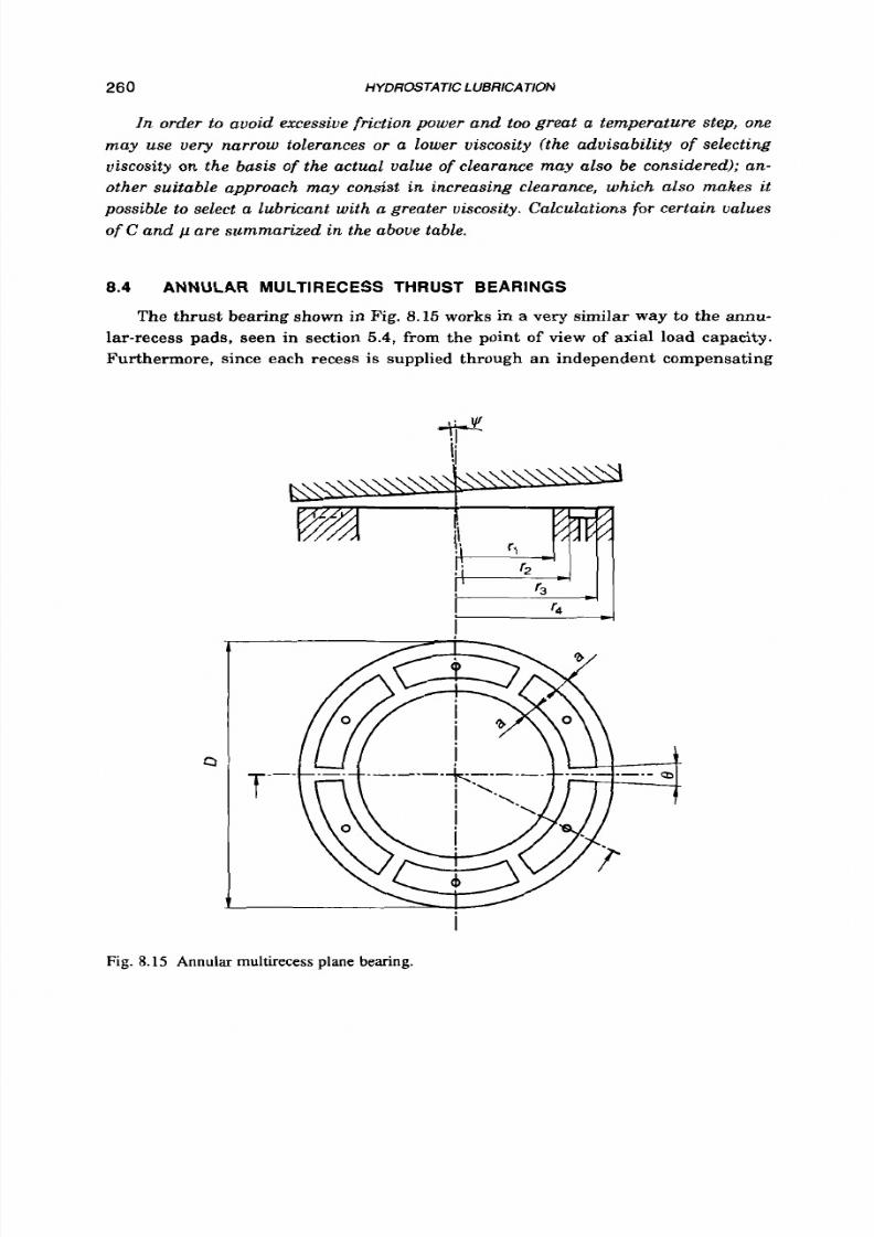
8/9/2019 Hydrostatic Lubrication 1992
http://slidepdf.com/reader/full/hydrostatic-lubrication-1992 277/558
260
HYDROSTATIC LUBRICATION
In order to avoid excessive friction power a nd too great a temperature step, one
may use very narrow tolerances or a lower viscosity (the advisability
of
selecting
viscosity on the basis of the actual value of clearance may also be considered); an -
other suitable approach may consist
in
increasing clearance, which also makes it
possible to select a lubricant with a greater viscosity. Calculations for certain values
of C and p are summa rized in the above table.
8.4
ANNULAR MULTIRECESS
THRUST
BEARINGS
The thrust bearing shown
in
Fig. 8.15 works in a
very
similar way to the annu-
lar-recess pads, seen in section 5.4, from the point of view of axial load capacity.
Furthermore, since each recess
is
supplied through an independent compensating
Fig. 8.15 Annular rnultirecess plane bearing.
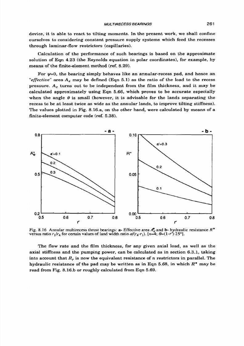
8/9/2019 Hydrostatic Lubrication 1992
http://slidepdf.com/reader/full/hydrostatic-lubrication-1992 278/558
MULTIRECESS
BEARINGS 261
device, it is able t o react t o tilting moments. In the present work, we shall confine
ourselves t o considering constant pressure supply systems which feed the recesses
through laminar-flow restrictors (capillaries).
Calculation of the performance of such bearings is based on the approximate
solution of Eqn 4.23 (the Reynolds equation in polar coordinates),
for
example, by
means of the finite-element method (ref. 8.29).
For y=O, he bearing simply behaves like an annular-recess pad, and hence an
effective area A, may be defined (Eqn 5.1) as the ratio of the load t o the recess
pressure.
A,
turns out t o be independent from the film thickness, and
it
may be
calculated approximately using Eqn 5.66, which proves
to
be accurate especially
when the angle
8 is
small (however, i t is advisable for the lands separating the
recess
to
be at least twice as wide as the annular lands,
to
improve tilting stiffness).
The values plotted in Fig. 8.16.a, on the other hand, were calculated by means of a
finite-element computer code (ref. 5.38).
- a - - b -
0.:
0.5 0.6
0.7
0.8
r'
0.00
'
0.5
0.6 0.7 0.8
r'
Fig. 8.16 Annular
multirecess thrust
bearings: a-
Effective
area
#,and b- hydraulic
resistance R*
versus
ratio r1/r4
for certain values
of
landwidth
ratio
cd(r4-t-I).[ n d , =(1-r?.25 ].
The
flow
rate and the film thickness, for any given axial load,
as
well as the
axial stiffness and the pumping power, can be calculated as in section 6.3.1, taking
into account that
R ,
is
now the equivalent resistance of
n
restrictors in parallel. The
hydraulic resistance of the pad may be written as in Eqn 5.68, in which R* may be
read from Fig. 8.16.b o r roughly calculated from Eqn 5.69.

8/9/2019 Hydrostatic Lubrication 1992
http://slidepdf.com/reader/full/hydrostatic-lubrication-1992 279/558
262 HYDROSTATIC LUBRICATION
In calculating the friction power, the contribution of the recess, mainly caused
by the damming effect of the radial lands, should be taken into account. Evaluating
it as in section 4.7 .3 , friction moment and friction power may still be expressed by
Eqn
5.70
and Eqn
5.72 ,
where:
Assuming h,.>>h and laminar flow, i.e. a Reynolds number
Re,. =$: O h ,
D
( 1 + r')
(8.36)
(8 .37)
less than
1000,
it may be stated that
f r=4h/h , .
A t high speed the effects of lubricant inertia become appreciable. Certain
numerical calculations are reported in ref. 8.30; although the data are presented in
a completely different form, a detailed analysis would show close agreement with
the results presented in section
5.4.5
for the continuous-recess pad (i.e. Eqn
5.77
to
Eqn
5 .80 ) .
Centrifugal forces cause an increase in flow rate, for a given recess pres-
sure, and, conversely, a decrease in recess pressure and load capacity when supply
pressure or flow rate are given.
As
has already been noted, the main distinguishing characteristic of these bear-
ings is their ability
t o
sustain tilting moments. Tilting stiffness, defined as the ratio
of the tilting moment M t t o angle
ry,
may be written as:
(8 .38)
The non-dimensional factor K ; is plotted in Fig. 8.17 (taken from ref. 8.31) as a func-
tion of the non-dimensional axial load WI A,ps and of the radius ratio r4/rl .A pres-
sure ratio /3=0.5 is clearly advisable, since it brings maximum stiffness both for ax-
ial and tilting loads.
Axial load capacity proves, in practice, t o be unaffected by a limited tilting an-
gle, at low speed; the problem may be quite different when til t is coupled t o high
speed. This kind of problem is dealt with in ref. 8.32 , in which Eqn 4.23 is solved, for
certain bearings. I t transpires that load capacity slightly increases with ti lt angle v
(thanks to the hydrodynamic effect), until cavitation occurs and load capacity breaks
down. For the bearings considered in the reference cited above [a '=0 .25 ; 8=30";
/3=0.5; il=(3/8)pLU I2/@,h2 )=50]his occurs a t y'=vD/ hz0.4 when
r'=0.4.
Higher val-
ues of
y'
could be allowed
for
r 5 0 . 5 .
However, the bearings considered i n ref.
8.32
are characterized by high values of power ratio
n,
hus, it may be concluded that, if
the bearing is designed on the usual basis
of
a power ratio Z7=Hf/Ht smaller than 3 ,
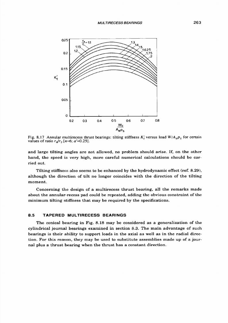
8/9/2019 Hydrostatic Lubrication 1992
http://slidepdf.com/reader/full/hydrostatic-lubrication-1992 280/558
MULTIRECESS BEARINGS
263
025
0.2
0.15
K;
0.1
0.05
0
\
0.2 0.3 0.4 0.5
0.6
0.7
0.8
4
A,P,
Fig.
8.17 Annular multirecess thrust bearings: tilting stiffness Ki versus load
WIA,p,
for certain
values of ratio
r&,.[n=6; a'=0.25].
and large tilting angles are not allowed, no problem should arise. If, on the other
hand, the speed is very high, more careful numerical calculations should be car-
ried out.
Tilting stiffness also seems
t o
be enhanced by the hydrodynamic effect (ref.
8.291,
although the direction of tilt no longer coincides with the direction of the tilting
moment.
Concerning the design
of
a multirecess thrust bearing, all the remarks made
about the annular-recess pad could be repeated, adding the obvious constraint of the
minimum tilting stiffness that may be required
by
the specifications.
8.5 TAPERED MULTIRECESS BEARINGS
The conical bearing in
Fig.
8.18 may be considered as a generalization of the
cylindrical journal bearings examined in section
8.3.
The main advantage of such
bearings is their ability to support loads in the axial a s well as in the radial direc-
tion. For this reason, they may be used
to
substitute assemblies made up of a jour-
nal plus a th rust bearing when the thrust has a constant direction.
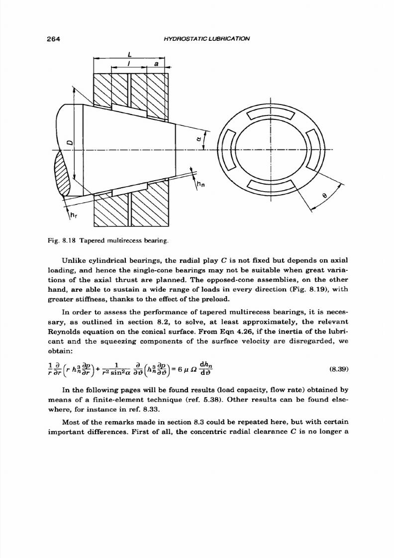
8/9/2019 Hydrostatic Lubrication 1992
http://slidepdf.com/reader/full/hydrostatic-lubrication-1992 281/558
264
HYDROSTATIC LUBRICATION
Fig. 8.18 Tapered multirecess bearing.
Unlike cylindrical bearings, the radial play C s not fixed but depends on axial
loading, and hence the single-cone bearings may not be suitable when great varia-
tions of the axial thrus t are planned. The opposed-cone assemblies, on the other
hand, are able t o sustain a wide range of loads in every direction (Fig. 8.191, with
greater stiffness, thanks to the effect of the preload.
In order to assess the performance of tapered multirecess bearings, it
is
neces-
sary, as outlined in section 8.2,
to
solve, at least approximately, the relevant
Reynolds equation on the conical surface. From Eqn
4.26,
if the inertia of the lubri-
cant and the squeezing components of the surface velocity are disregarded, we
obtain:
In the following pages
will
be found results (load capacity,
flow rate)
obtained by
means of a finite-element technique (ref. 5.38). Other results can be found else-
where, for instance in ref, 8.33.
Most
of the remarks made in section 8.3 could be repeated here, but with certain
important differences. First of all, the concentric radial clearance
C
s no longer a

8/9/2019 Hydrostatic Lubrication 1992
http://slidepdf.com/reader/full/hydrostatic-lubrication-1992 282/558
MUL
TIRECESS
BEARINGS 265
constant, being related to the axial film thickness, i.e. t o the axial load. Conse-
quently, the actual value of the concentric pressure ratio
p
also depends on the
axial
load.
As for the other multirecess bearings, we shall concentrate on the most com-
mon constant-pressure supply systems, with capillary compensation.
- a -
_-
- b -
- c -
--
Fig. 8.19 Arrangements
of
tapered multirecess bearings.
8.5.1 Slngle-cone journal bear ings
Let us begin by examining the performance of the single-cone bearings, fed by
means of laminar-flow restrictors. If no radial load is present (i.e. it is E=O ) , axial
load capacity may be written in the following form:
Wz =A,
pr
= A,
P Ps
(8.40)
where, as usual, A,
is
the effective bearing area and
p
is the concentric pressure
ratio. A, may be considered to be a constant. At least when no radial load is applied,
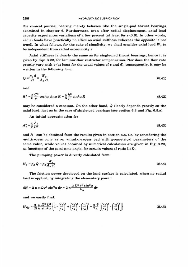
8/9/2019 Hydrostatic Lubrication 1992
http://slidepdf.com/reader/full/hydrostatic-lubrication-1992 283/558
266 HYDROSTATIC LUBRlCATlo N
the conical journal bearing merely behaves like the single-pad thrust bearings
examined in chapter
6.
Furthermore, even after radial displacement, axial load
capacity experiences variations of a few percent (at least for ~<0.6).n other words,
radial loads have practically no effect on axial stiffness (whereas the opposite is not
true ). In what follows, for the sake of simplicity, we shall consider axial load
W, o
be independent from radial eccentricity
E.
Axial stiffness
is
clearly the same as for single-pad thrust bearings; hence
it
is
given by Eqn
6.22,
for laminar-flow restrictor compensation. Nor does the
flow
rate
greatly vary with E (at least for the usual values of E and
B) ;
consequently, it may be
written in the following form:
P B w,
Q=*=m
and
(8.41)
(8.42)
may be considered a constant. On the other hand,
Q
clearly depends greatly on the
axial load, just as in the case of single-pad bearings (see section
6.3
and Fig. 6.5.a).
An initial approximation for
(8.43)
and R* an be obtained from the results given in section 5.5, i.e. by considering the
multirecess cone as an annular-recess pad with geometrical parameters of the
same value, while values obtained by numerical calculation are given in Fig. 8.20,
as functions of the semi-cone angle, for certain values of ratio LI D.
The pumping power
is
directly calculated from:
(8.44)
The friction power developed on the land surface is calculated, when no radial
load is applied, by integrating the elementary power
and we easily find:
(8.45)

8/9/2019 Hydrostatic Lubrication 1992
http://slidepdf.com/reader/full/hydrostatic-lubrication-1992 284/558
MULTIRECESS BEARINGS 267
0.0
0.e
0.6
A',
0.4
0.2
0.00
- a -
0.15
R'
0.10
0.05
a
- b -
UD=1 I I 0.75
I
/
1 0 . 5
15" 30" 45"
a
Fig.
8.20
Tapered multirecess bearings: a- Effective area A*,
and
b- hydraulic resistance R* ver-
sus
semi-cone
angle a
or
certain values of ratio LID;
(n=4,
=30°).
Friction power, of course, varies with the eccentricity, but
it
is
often enough for
the designer t o consider the value above alone.
When the recesses are large, their contribution
t o
friction should also be taken
into account. Proceeding as in the case of the journal bearings (sect. 8.3.11,we find:
(8.46)
where
it
may be stated that fr=4h,lh, if h,>>h, and the Reynolds number in the
recess
I P
L
2 P
e =
-
-
, D 2
(1
-
tga)
is
smaller than
1000.
The friction power may now be written as follows:
(8.47)
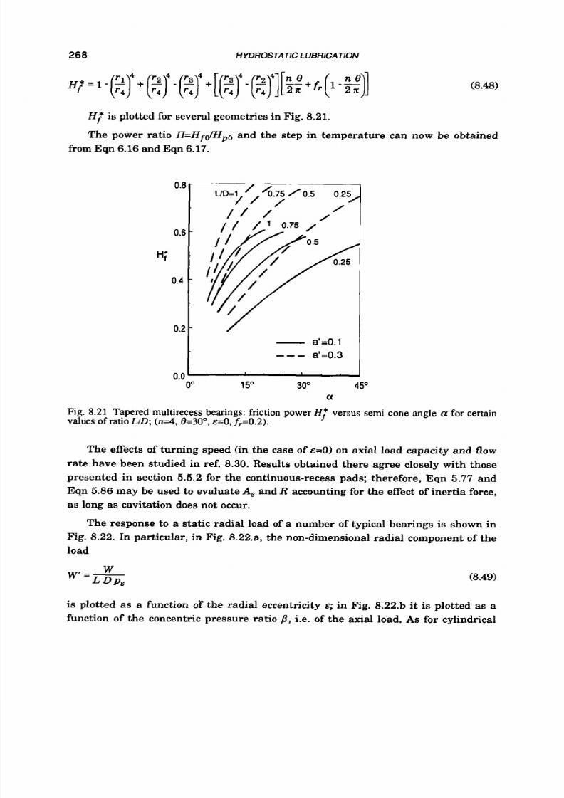
8/9/2019 Hydrostatic Lubrication 1992
http://slidepdf.com/reader/full/hydrostatic-lubrication-1992 285/558
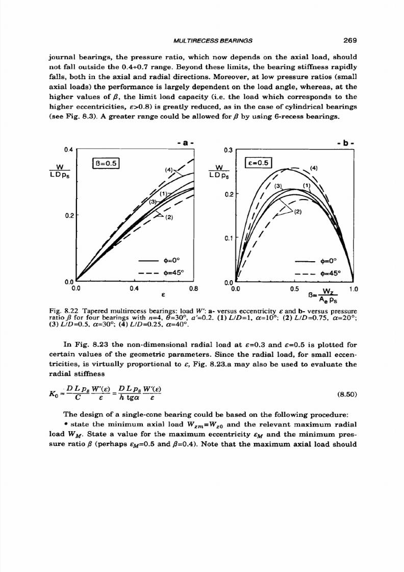
8/9/2019 Hydrostatic Lubrication 1992
http://slidepdf.com/reader/full/hydrostatic-lubrication-1992 286/558
MULTIRECESS
BEARINGS
269
journal bearings, the pressure ratio, which now depends on the axial load, should
not fall outside the 0.4t0.7 range. Beyond these limits, the bearing stiffness rapidly
falls, both in the axial and radial directions. Moreover, at low pressure ratios (small
axial loads) the performance is largely dependent on the load angle, whereas, a t the
higher values of p, the limit load capacity (i.e. the load which corresponds to the
higher eccentricities,
~>0.8)
s greatly reduced, as in the case of cylindrical bearings
(see Fig. 8.3).
A
greater range could be allowed for p by using 6-recess bearings.
- a -
0.4
0.0
0.4 0.8
E
0.3
W
-
L D Ps
0.2
0.1
0.0
- b -
0.0 0.5 1 o
0- J h-
A, Ps
Fig. 8.22 Tapered multirecess bearings: load W': a- versus eccentricity
E
and b- versus pressure
ratio4 for four bearings
with
n=4,
8=30°,
a'=0.2. (1)LID=l . a=lOO; 2) LID=0.75, a=20°;
(3)
LID=O.5,
a=3Oo;
4) LID=O.25,
a=40°.
In Fig. 8.23 the non-dimensional radial load at
~ = 0 . 3
nd ~ = 0 . 5s plotted for
certain values of the geometric parameters. Since the radial load, for small eccen-
tricities, is virtually proportional to E, Fig. 8.23.a may also be used to evaluate the
radial stiffness
D
L
p SW ( E ) D
L
p S
WYE)
KO =
-
C
E h t g a E
(8.50)
The design of a single-cone bearing could be based on the following procedure:
state the minimum axial load
W z m = W z o
and the relevant maximum radial
load WM. tate a value for the maximum eccentricity EM and the minimum pres-
sure ratio /3 (perhaps eM=0.5and
p=0.4).
Note that the maximum axial load should

8/9/2019 Hydrostatic Lubrication 1992
http://slidepdf.com/reader/full/hydrostatic-lubrication-1992 287/558
270
HYDROSTATIC LUB RlCAT/ON
- a -
I
- b
0.4 I
0.2
-
w
0.1
-
- '=0.1
- - - a'=0.3
0.0
0"
1
5" 30" 45"
a
0.3
w
0.2
0.1
\
\0 .75
\ 1 '
\
V .
0" 15 30" 45
a
Fig.
8.23
Tapered multirecess bearings: load W versus semi-cone angle
a
for: a- eccentricity
~ = 0 . 3 ,nd b- ~ 4 . 5 ;n=4, 9=30°,J=0.4,
4 4 5 ) .
not exceed
1.75.W,,,
otherwise the pressure ratio under the highest load may prove
to be too high to give good radial stiffness;
assume a/L=O.l (a greater value is, however, suitable for slowly rotating bear-
ings). Select (for example with the help
of
Fig. 8.241 the aperture angle a and the
length to diameter ratio LID;
the bearing can now be calculated just like a single-pad thrust bearing
(section 6.4.21,except that, in selecting the film thickness, the required radial stiff-
ness must also be considered. In other words, it must be
eM
C
=
h t g a s -
EM
where eM is the maximum allowable value
of
the radial displacement. "Optimal"
values
of
the viscosity and pumping power are given by Eqn
6.56
and Eqn
6.57.
Figure
8.25
contains plots of
HF
and
p; for
certain bearing shapes.
8.5.2
Opposed-cone assembl ies
Let us now consider an opposed-cone assembly, such as those in Fig. 8.19. The
axial play 2ho is established during manufacturing (although plans can be made to

8/9/2019 Hydrostatic Lubrication 1992
http://slidepdf.com/reader/full/hydrostatic-lubrication-1992 288/558
M U L
TIRECESS
B EARlNGS 271
adjust it during assemblage); hence, the radial play at
W,=O
s Co=hotga
or
both
cones. The concentric pressure ratio is
1
R ,
p
1+-
n
R* h: sin3a
(8.51)
where
R,
is the hydraulic resistance of each restrictor and n the number of recesses
of each cone: the two cones are assumed t o be identical.
1
.I
-
wz
02
- a -
0.1
0" 15 30 45
a
- b -
0.c
0 15 30 45
a
Fig.
8.24
Tapered multirecess bearings: ratio of radial load W to axial load
W,
versus semi-cone
angle a for: a- eccentricity
~ = 0 . 3 ,
nd b- ~ = 0 . 5 ;n=4, 0=30",&0.4, 4=45 ).
In this case, the response to an axial load is the same as tha t of the opposed-pad
bearings, that is:
wz
= A, Ps w;v;
(8.52)
K
=KO
K&3;
&,I
where:
(8.54)
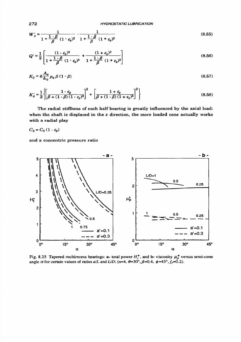
8/9/2019 Hydrostatic Lubrication 1992
http://slidepdf.com/reader/full/hydrostatic-lubrication-1992 289/558
272
HYDROSTATIC LUBRICATION
1 1
w; =
I+? ( 1 - ~ 3 +? ( 1 + . ~ 3
(8.55)
(8.58)
The radial stiffness of each half bearing is greatly influenced by the axial load:
when the shaft
is
displaced in the z direction, the more loaded cone actually works
with a radial play
c, = c, (1
-
4)
and a concentric pressure ratio
5
4
3
";
2
1
- a -
1 0.75
-
'=0.1
_ _ -
' 4 . 3
0
0
15
30 45
a
3
2
6
1
0
- t
UD=1
0.25
\,
0.5,
15 30'
45
a
Fig. 8.25 Tapered multirecess bearings:
a-
total power H: . and b- viscosity
p;
versus semi-cone
angle
a
or certain values of ratios alL and Y D ; n 4 , 9=30°,&0.4,
$ 4 5 ' ,
fr=0.2) .
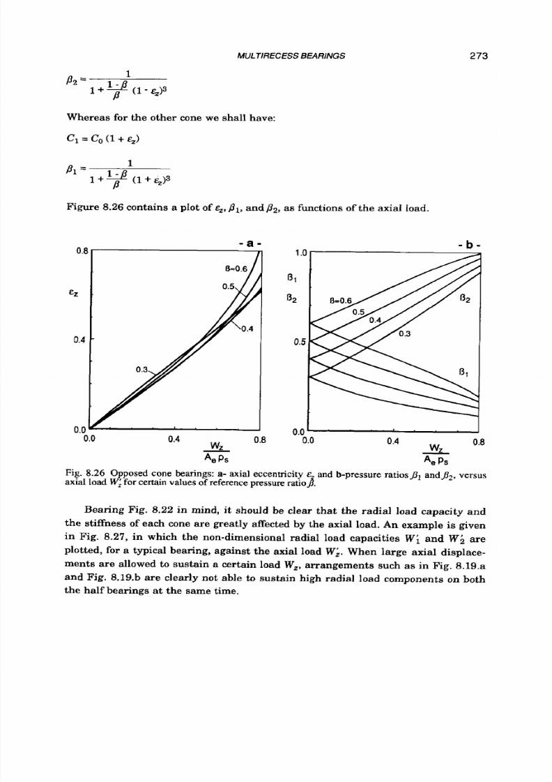
8/9/2019 Hydrostatic Lubrication 1992
http://slidepdf.com/reader/full/hydrostatic-lubrication-1992 290/558
MULTIRECESS BEARINGS
273
1
8 2
=
I + $ - @
( 1 - ~ 3
Whereas for the other cone we shall have:
c1=
c, 1 + &,I
Figure 8.26 contains a plot of G,
1,
and &, as functions of the axial Ioad.
- a -
0=0.6
I
0.0 0.4
0.8
w
A, Ps
0 . 0 " ' " . ' '
0.0
0.4 0.8
w
A, Ps
Fig.
8.26
Opposed cone bearings:
a-
axial eccentricity
&
and b-pressure ratiosJ1 and&, versus
axial load W;
or
certain values of reference pressure ratioj.
Bearing Fig. 8.22 in mind, it should be clear that the radial load capacity and
the stiffness of each cone are greatly affected by the axial load. An example is given
in Fig. 8.27, in which the non-dimensional radial load capacities W i and
W;
are
plotted, for a typical bearing, against the axial load Wl. When large axial displace-
ments are allowed
to
sustain a certain load W,, rrangements such as in Fig. 8.19.a
and Fig. 8.19.b are clearly not able
to
sustain high radial load components on both
the half bearings a t the same time.
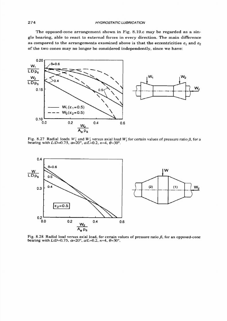
8/9/2019 Hydrostatic Lubrication 1992
http://slidepdf.com/reader/full/hydrostatic-lubrication-1992 291/558
2 7 4
HYDROSTATIC LUB RICATION
The opposed-cone arrangement shown in Fig. 8.19.c may be regarded as a sin-
gle bearing, able
t o
react to external forces in every direction. The main difference
as compared to the arrangements examined above
is
that the eccentricities and
~2
of
the two cones may no longer be considered independently, since we have:
0.0 0.2
0.4
0.6
w
Ae
PS
Fig.
8.27 Radial loads
W ;
and
W ;
versus axial load
W; for
certain values
of
pressure ratio$, for a
bearing with
L I D 4 . 7 5 ,
a=2Oo,
alL=0.2,
n=4,
0=30°.
0.4
-
.-
0.0
0.2 0.4
w
0.6
Ae
PS
Fig.
8.28
Radial load versus axial load. for certain values
of
pressure r a t i o j , for an opposed-cone
bearing
with
L I D 4 . 7 5 .
a=20°,
a/L=0.2,
n=4.
8=30°.

8/9/2019 Hydrostatic Lubrication 1992
http://slidepdf.com/reader/full/hydrostatic-lubrication-1992 292/558
MULTIRECESS
BEARINGS
275
The radial load capacity is,
of
course,
W=W,+W2.
When an axial load is applied,
becomes smaller than
E,,
and hence the radial load capacity is mainly due to W,.
Figure 8.28 shows, by way
of
example, how the radial load capacity of a given bear-
ing is affected by a radial component
W,.
8.6
SPHERICAL JOURNAL BEARINGS
Spherical multirecess bearings (Fig. 8.29) have the advantage,
as
compared to
similar conical types, of being intrinsically insensitive
to
the tilting misalignment of
the journal. On the other hand, they are more difficult and more expensive
t o
build.
Fig. 8.29 Spherical journal bearing.

8/9/2019 Hydrostatic Lubrication 1992
http://slidepdf.com/reader/full/hydrostatic-lubrication-1992 293/558
276 HYDROSTATICLUBRICATlON
To evaluate the performance of such bearings, the relevant Reynolds equation
(Eqn 4.30) should be solved numerically. Due t o the large number of geometrical
parameters, general charts are not given, but in Fig. 8.30 (obtained from ref. 8.34,
as are the following figures in this section) the main performance of
a
typical 6
recess bearing is shown. In more detail, in Fig. 8.30.a, the axial and radial compo-
nents of the load, i.e. W, and W, are plotted as functions of the eccentricity
E
and the
relevant angle whereas the effect of the attitude angle is small. In Fig. 8.30.b the
flow rate for W=O:
(8.59)
is given as
a
function of E. The pressure ratio in the concentric position is assumed
to be p=0.5. As usual, this value is considered t o be the optimal one, when fixed
laminar restrictors
a r e
used as compensating devices, from the point of view of both
axial and radial stiffness. Furthermore, for different values of p, higher interaction
occurs between the loads in the axial and radial directions, whereas from Fig. 8.30
it is clear that the axial load has little influence on radial stiffness, a t least when yis
between 60"and 90 . In Fig. 8.31.a the effect o fa on load capacity a t ~= 0 . 5nd on the
concentric flow rate is shown for the same bearing as in Fig. 8.30.
Concerning the geometrical parameters, ref. 8.34 shows that
t o
decrease rp, t o
below 30" has a detrimental effect on radial load capacity.
It
may be advisable
t o
use
- a -
-
b-
12
Q'
8
4
0.04 0.1
-
Ps
D'
0
Fig. 8.30
a-
Load-displacement characteristics;
b-
flow rate versus eccentricity, for a spherical
bearing
with 'pl=5Oo, 2=850 , qa=8=3S0,n=6.J=0.5 (ref. 8.34).

8/9/2019 Hydrostatic Lubrication 1992
http://slidepdf.com/reader/full/hydrostatic-lubrication-1992 294/558
MULTIRECESS BEARINGS 277
larger lands than for the bearing considered above; radial load capacity is virtually
unaffected by an increase
t o
0.25-((p4-(pl)f the width of the axial and radial lands,
while the reduction in axial load capacity is largely compensated by the decrease in
flow
rate. With reference
t o
Fig. 8.31.b, the non-dimensional axial load capacity
is
clearly reduced by a factor
0.9
when passing from a land angle of 3.5"
t o a
land
angle
of 7".
This may be compensated by a reciprocal variation in supply pressure.
On the other hand, the non-dimensional
flow
rate
is
halved; consequently, taking
the pressure increase into account, the actual
flow
rate will be reduced by almost
44%, and pumping power by 38%. Furthermore, thanks
t o
the small increase in
supply pressure, the radial stiffness will also actually be better.
- b -
0.2 I I
W (0.5, 0°)
W
D2P s
20
10
0.0
0.10 0.15 0.20 0.25
'Pa
92-91
Fig.
8.31
Axial load, radial load and flow rate versus a- pressure ratio and b- land width ratio,
for a spherical bearing
with (pl=500,p2=850, n=6
(ref.
8.34).
Friction power may be roughly calculated, in the concentric position E=O, by the
equation:
This last equation was obtained on the assumption that the recess depth
hr is
much greater than the radial clearance C. For the friction coefficient f, i t may be
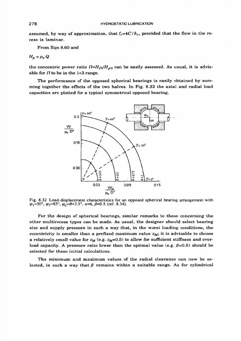
8/9/2019 Hydrostatic Lubrication 1992
http://slidepdf.com/reader/full/hydrostatic-lubrication-1992 295/558
278 HYDROSTATIC
1
UBRICA TION
assumed, by way of approximation, that f r = 4 C l h r ,provided that the flow in the re-
cess is laminar.
From Eqn 8.60 and
H p = p s Q
the concentric power ratio 17=HfdHpo can be easily assessed.
As
usual,
it
is advis-
able for
II
to be in the li-3 range.
The performance of the opposed spherical bearings i s easily obtained by sum-
ming together the effects of the two halves. In Fig. 8.32 the axial and radial load
capacities are plotted for a typical symmetrical opposed bearing.
03
0.18
0 6
0.03
0.09 015
-
Z
Ps D2
Fig. 8.32 Load-displacement characteristics for an opposed spherical bearing arrangement
with
'pl=5O0, 'p2=85",
( ~ , = 8 = 3 . 5 ~ ,
=6,J=0.5
(ref. 8.34).
For the design of spherical bearings, similar remarks to those concerning the
other multirecess types can be made. As usual, the designer should select bearing
size and supply pressure in such a way that, in the worst loading conditions, the
eccentricity is smaller than
a
prefixed maximum value
EM;
it is advisable to choose
a relatively small value for EM (e.g.
~ ~ = 0 . 5 )
o allow for sufficient stiffness and over-
load capacity. A pressure ratio lower than the optimal value (e.g. 8=0.5) should be
selected for these initial calculations.
The minimum and maximum values of the radial clearance can now be se-
lected, in such a way that
p
remains within a suitable range. As for cylindrical
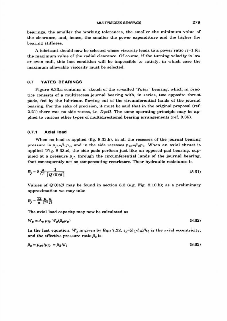
8/9/2019 Hydrostatic Lubrication 1992
http://slidepdf.com/reader/full/hydrostatic-lubrication-1992 296/558
MULTIRECESS
BEARINGS
279
bearings, the smaller the working tolerances, the smaller the minimum value of
the clearance, and, hence, the smaller the power expenditure and the higher the
bearing stiffness.
A
lubricant should now be selected whose viscosity leads
to
a power ratio
n = 1
for
the maximum value of the radial clearance. Of course, if the turning velocity is low
o r even null, this last condition will be impossible to satisfy, in which case the
maximum allowable viscosity must be selected.
8.7
YATES
BEARINGS
Figure 8.33.a contains a sketch of the so-called "Yates" bearing, which in prac-
tice consists of a multirecess journal bearing with, in series, two opposite thrust
pads, fed by the lubricant flowing out of the circumferential lands of the journal
bearing. For the sake of precision, it must be said that in the original proposal (ref.
2 .21 )
there was no side recess, i.e.
Di=D.
The same operating principle may be ap-
plied
t o
various other types of multidirectional bearing arrangements (ref. 8.35).
8.7.1 Axia l load
When no load is applied (fig. 8.33.b), in all the recesses of the journal bearing
pressure is
p j o = p l p , ,
and in the side recesses
p z 0 = P 2 p s .
When an axial thrust is
applied (Fig. 8.33.c), the side pads perform just like an opposed-pad bearing, sup-
plied at a pressure p j o through the circumferential lands of the journal bearing,
that consequently act as compensating restrictors. Their hydraulic resistance is
(8.61)
Values of Q'(O)/jl may be found in section 8.3 (e.g. Fig. 8.10.b); as a preliminary
approximation we may take
The axial load capacity may now be calculated as
wz = A , Pjo w;(a,; ) (8.62)
In the last equation,
W;
s given by Eqn
7 . 2 2 ,
~~=(h~-hO)lhos the axial eccentricity,
and the effective pressure ratio
8,
is
Pz =
Pzo
lPj0 =
82
18 1
(8.63)
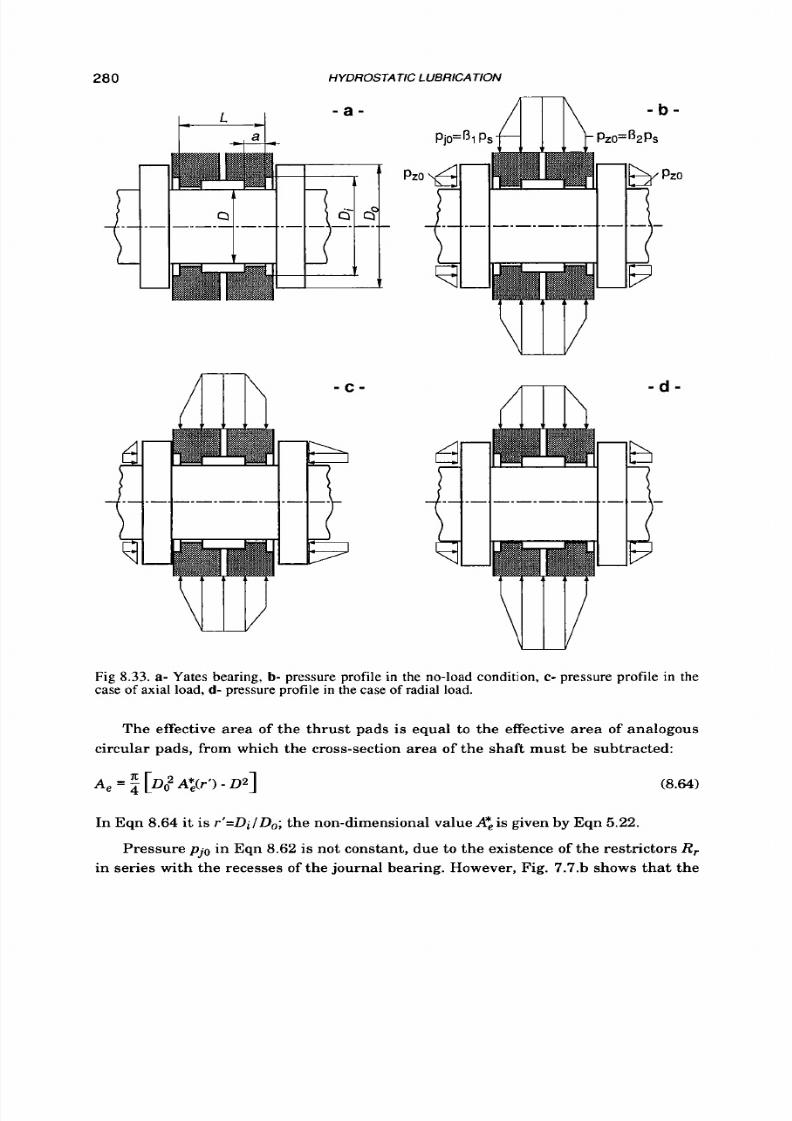
8/9/2019 Hydrostatic Lubrication 1992
http://slidepdf.com/reader/full/hydrostatic-lubrication-1992 297/558
280
HYDROSTA
- a -
t+zi
- c -
m
,TIC
LUBRICATION
- b -
Fig
8.33.
a- Yates bearing, b- pressure profile in the no-load condition,
c-
pressure profile in the
case of axial load, d - pressure profile in the case of radial load .
The effective area of the thrust pads is equal to the effective area of analogous
circular pads, from which the cross-section area of the shaft must be subtracted:
A, = 2 [DO"
A*,(r') 0 2 1
(8.64)
In Eqn
8.64
it is
r'=Di/D,;
the non-dimensional value A*,is given by Eqn
5.22.
Pressure
pjo
in Eqn
8.62
is not constant, due to the existence of the restrictors
R,
in series with the recesses of the journal bearing. However, Fig. 7.7.b shows tha t the

8/9/2019 Hydrostatic Lubrication 1992
http://slidepdf.com/reader/full/hydrostatic-lubrication-1992 298/558
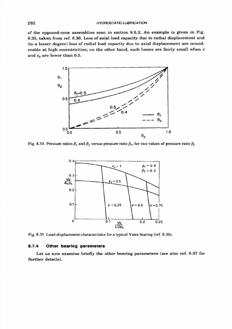
8/9/2019 Hydrostatic Lubrication 1992
http://slidepdf.com/reader/full/hydrostatic-lubrication-1992 299/558
282
HYDROSTATIC L UBRICATlON
of the opposed-cone assemblies seen in section 8.5.2.An example is given in Fig.
8.35, aken from ref. 8.36.Loss of axial load capacity due to radial displacement and
(to a lesser degree) loss of radial load capacity due t o axial displacement are consid-
erable at high eccentricities; on the other hand, such losses are fairly small when
E
and
E,
are lower than 0.5.
Fig. 8.34 Pressure ratiosfl, andJ2 versus pressure ratioJz, for two values
of
pressure ratioJj,
0.3
-
0.2-
0
0.1
w 0.2
0.25
..
L
DP,
Fig. 8.35 Load-displacement characteristics for a typical Yates bearing (ref. 8.36).
8.7.4
Other
bearing
parameters
Let us now examine briefly the other bearing parameters (see also ref. 8.37 for
further details).

8/9/2019 Hydrostatic Lubrication 1992
http://slidepdf.com/reader/full/hydrostatic-lubrication-1992 300/558
MULTIRECESS
BEARINGS 283
Flow rate in the reference configuration E=G=O is easily calculated from Eqn
8.11
or Eqn
7.23
(8.69)
where R* is given by Eqn 5.23.When any load
is
applied, flow rate should be slightly
smaller, if both Pj and P, are lower than 0.5. Pumping power is
H p o
=~s QO
(8.70)
Friction may be evaluated by summing the effects due to the journal and to the
side pads. In the unloaded configuration we find with no difficulty that
(8.7
)
Factors + nd H; may be calculated by means of Eqn
8.23
and Eqn
5.27,
respec-
tively. It should be noted that C and ho cannot be chosen in a completely indepen-
dent fashion, since in order to obtain the selected values of the pressure ratios we
must have
(8.72)
The power loss due to friction is easily calculated by multiplying the friction
moment by the angular speed
HfO = MfO a
(8.73)
8.7.5 Design procedure
The design
of
a Yates bearing is not very different from the design of journal
and opposed-pad bearings.
Once the maximum values of the load components are given, the first step con-
sists in selecting the values of the pressure ratios (see Fig.
8.34);
t should be taken
into account that PjeO.5 is the optimum for the radial stiffness (however, values
smaller than
0.4
should be avoided). as far as p , is concerned, selecting too small a
value would give poor axial stiffness; on the contrary, too high values lead to poor
radial load capacity (since it is proportional to
1-PZ)
nd even the axial stiffness
breaks down when is close
to
unit.
A
typical selection might be
&=0.2,
and
p1=0.6;
possibly, both may be increased in order to increase the axial load capacity; the
opposite may be done when the radial load is more critical.
8/9/2019 Hydrostatic Lubrication 1992
http://slidepdf.com/reader/full/hydrostatic-lubrication-1992 301/558
284 HYDROSTATIC LUBRICA TlON
The next step may consist in dimensioning the journal bearing (see
also
section
8.3.3).After suitable trial values for a / Land L I D (say a/L=0.1and L I D = l )have been
stated, diameter D and supply pressure p s may be calculated by means of Eqn 8.68.
In designing
it
may be best to slightly increase loads (perhaps by
10%)
o
account for
the losses in load capacity due to interactions between thrust and radial load. The
radial clearance C may then be selected; as usual, the narrower
C
s the higher
radial stiffness will prove t o be and the lower the total power consumption (provided
that
it
is possible t o select a lubricant with a viscosity close to the relevant
"optimal"
value).
The thrust bearing may now be designed (see also section 7.2.6). First, one may
choose the radius ratio
r'
(say r'=0.9); n general, thin lands are more convenient,
unless
R
is very slow. The axial gap
ho
may not be chosen at
will
but must be calcu-
lated by means of Eqn 8.72; should i t prove t o be
too
narrow, it might be necessary
t o
reduce r'; on the contrary, if ho seems too thick, causing poor axial stiffness, it may
be necessary to reconsider the journal bearing, increasing a IL . The effective area
needed
t o
sustain the axial load may be calculated by means of Eqn
8.65,
and then
the outer diameter Do by means of Eqn 8.64. Should the axial load be small, it could
turn out that
Di=r'D@:
in this case a smaller value can be chosen for
E ~ ,
s well as
for 81 nd
8 2 .
The selection of the "optimal" value of viscosity will be based, as usual, on the
power ratio
17=HfdHpo.
From Eqn 8.70 and Eqn 8.73 one may obtain
(8.74)
in which one should state l7=1 o obtain the optimal viscosity.
As
for the other bear-
ing types considered in previous sections, it may happen than this calculated viscos-
ity is
too
low or too high; the remedies are, of course, similar: increase film thick-
ness and
I l
in the former case (avoid, however, values of
Il
greater than
3);
increase
the land width and decrease I7 in the latter case. When the viscosity value is a con-
straint, the same Eqn 8.74 allows us to select clearance C in such a way as
t o
get a
power ratio in the l t 3 range.
Once the main bearing parameters have been established,
it is
possible to calcu-
late
flow
rate, friction torque, and the relevant power losses. It
is
also advisable
to
check the Reynolds numbers and the temperature steps, as in the case of the other
bearings. Finally, the hydraulic resistance of each of the
n
restrictors R, which
compensates recess pressures in the journal bearing has t o be

8/9/2019 Hydrostatic Lubrication 1992
http://slidepdf.com/reader/full/hydrostatic-lubrication-1992 302/558
MULTIRECESS
BEARINGS 285
where Rj may be calculated by means
of
Eqn 8.61.
One final remark: it should be noted that the actual values of
C
and
ho
have a
considerable influence of the loading performance of the assembly. For instance, let
us assume that radial clearance proves
t o
be greater than the selected value
C ,
while all the other remain the same; consequently, the resistance of the lands
of
the
journal bearing (proportional to
C - 3 )
will be lower, and we actually get a smaller
value
of P I ,
and a greater value of
Icj2,
i.e. both axial and radial load capacities have
been lowered. Of course, if clearance is narrower than designed, and p 2 change
in the opposite way; nevertheless, stiffness may become very poor, since Bj and 0,
differ from their optimal values.
R E F E R E N C E S
8.1
82
8.3
8.4
8.5
8.6
8.7
8.8
8.9
8.10
8.11
8.12
O'Donoghue
J. P.,
Hooke C. J., Rowe
W.
B.; A Solution Using Superposit ion
Technique for Externally Pressurized Multirecess Jour nal Bearings Includ -
ing Hydrodynamic Effects;Proc. Instn. Mech. Engrs.; 185,5 (1970-71), 57-61.
Colsher R., Anwar I., Katsumata S.;
An Advanced Method fo r Predict ing
Hybrid Bearing Performance; AGARD Conf. Proc. 323, 1982, paper 28;
13
pp.
Ghai R. C., Singh D.
V.,
Sinhasan R.; Load Capacity and Flow Characteris-
t ics of a Hydrostatically Lubricated Four-Pocket Journ al Bearing by Finite
Element Method;
Int.
J .
Mach. Tool Des Res, 16 (19761, 233-240.
Shapiro W.;
Computer-Aided Design of Externally Pressurized Bearings;
Instn. Mech. Engrs., C
10/71
(1971); 22 pp.
Raimondi
A.
A., Boyd J.; An
Analysis of Orifice an d Capillary Com pensated
Hydrostatic Journa l Bearings; Lubr. Eng., 13 (1957), 28-37.
Kher A. K., Cowley A,; Th e Design and Performance C haracteristics of a
Capillary Compensated Hydrostatic Journal Bearing;
Proc. 8th Int. MTDR
Davies P. B.; A
General Ana lysis o f Multirecess Hydrostatic Journ al Bear-
ings;
Proc.
Instn. Mech. Engrs.; 184,l (1969-701, 827-836.
Bettini B.;
Calcolo d i Cuscinetti Ra dia li Zdrostatici; Progetto d i una Attrez-
zatura d i Prova; Doct. Thesis, 1985; 269 pp.
Singh D. V., Sinhasan R., Ghai R. C.; Finite Element Analysis of Orifice
Compensated Hydrostatic Jo urnal Bearings;
Tribology Int. ,
9
(1976), 281-284.
Sinhasan R., Sharma S. C., Jain S. C.;
Performance Charac ter ist ics o f a
Constant Flow Value Compensated Multirecess Flexible Hydrostatic Journal
Bearing;
Wear, 134 (19891,335-356.
Davies P. B.; Th e Dynamic Behaviour of Passively Compensated, Hydrostatic
Journal Bear ings w i th Var ious Nu mb er of Recesses;
J. of Mech. Eng. Sci-
ence,
18
(19761,292-302.
Rowe
W. B.; Dynamic and Static Properties of Recessed Hydrostatic Journal
Bear ings by Small Displacement Analys is ; ASME Trans, J . of Lubrication
Technology, 102 (1980), 71-79.
Co d. (1967), pt. 1,397-418.
8/9/2019 Hydrostatic Lubrication 1992
http://slidepdf.com/reader/full/hydrostatic-lubrication-1992 303/558
HYDROSTATIC LUBRICATION
Ho Y. S.,
Chen N. N.
S.; Performance Characteristics of a Capillary-Con-
pensated Hydrostatic Journal Bearing;
Wear, 52 19791,285-295.
Lingard
S.,
hen N. N.
S.,
Kong Y. C.;
Aspects of the Performance of Exter-
nally Pressurized Journal Bearings; Wear, 78 19821,343-353.
Ar tiles A., Walowit J. , S hap iro W.;
Analysis of Hybrid, Fluid-Film Journal
Bearings with Turbulence and Znertia Effects;
Advances in Computer-Aided
Be arin g Design, ASME-ASLE Lubrication conf., Washington D.C., 1982;
p.
Manea G.; Machine Elements; Technical Publishing House, Bucharest; 1970.
D um bra w a M. A.;
Review of Principles and Methods Applied to the Optimum
Calculation and Design of Externally-Pressurized Bearings. Part 1:
Low /Moderate Speed Bearings;
Tribology Int., 18 19851, 149-156.
Dumbrawa M. A.;
Review of Principles and Methods Applied to the Optimum
Calculation and Design of Externally-Pressurized Bearings. Part 2: Moder-
atelHigh-Speed Bearings;
Tribology Int.,
18
1985), 223-228.
Rowe W. B., Koshal D., Stout K. J.; Investigation of Recessed Hydrostatic and
Slot-Entry Journal Bearings for Hybrid, Hydrodynamic and Hydrostatic
Operation;
Wear, 43 (19771,55-69.
El She rb iny M., Sa lem F., El Hefnawy N.;
Optimum Design of Hydrostatic
Journal Bearings. Part 2: Minimum Power;Tribology
Int., 17 19841, 162-166.
Vermeulen M.; Optimisation of Hydrostatic Journal Bearings Zncluding
Hydrodynamic Effects;
Proc. Euro trib 81, Varsaw, 1981;V. 2, pp. 371-388.
Hydrostatische Radial-Gleitlager im Stationaren Betrieb (Berechnung von
Olgeschmierten Gleitlagern ohne Zwischennuten);
DIN 31655, Teil 1, Nov.
1984; 29
p.
Hydrostatische Radial-Gleitlager im Stationaren Betrieb (Kenngropen fur die
Berechnung von Olgeschmierten
Gleitlagern ohne Zwischennuten);
D I N
31655,Te il2 , Nov. 1984; 11 p.
Rowe W. B., Stout K.
J.; The Design of Externally Pressurized Bearings for
Reliability with Particular Reference to Manufacturing Errors; Instn. Mech.
Engrs.; C310 19731,421-429.
X u S.,
Chen B.;
Optimum Design and Automatic Drawing
of
Recessed Hy-
drostalCc Bearings;
Tribological Design
o f
Machine Elements , p roc .
15 th
Leeds-Lyon Sym p. on Tribology, Leeds, 1988;p. 411-418.
O'Donoghue
J.
P., Rowe W. B., Hooke C.
J.;
Some Tolerancing Effects in
Hydrostatic Bearings;Proc. 11th In t . MTDR Co d. (1970);pp. 317-322.
Sa to Y., Ogiso
S.;
Load Capacity and Stiffness of Misaligned Hydrostatic
Recessed Journal Bearings;
Wear, 92 1983), 231-241.
Moshin M. E.;
A Hydrostatic Bearing for High Speed Applications;
Tribology
Int., 14 1981),47-54.
Aoyama T., Inasaki I., Yonetsu
S.; Friction and Tilting Characteristics of
Hydrostatic Thrust Bearings;
Bull . Japan
SOC.
f Precision Eng., 10 19761, 68-
70.
P r a b h u
T.
J. , Ganesan N.;
Analysis
of
Multirecess Conical Hydrostatic
Thrust Bearings under Rotation;
Wear,
89
19831, 29-40.
O'Donoghue
J.
P.;
Design
of
Annular Multi-Recess Hydrostatic Thrust
Bearings;
Mach. a n d Prod. Eng., Nov. 18, 1970; p. 830-834.
25-51.
286
8.13
8.14
8.15
8.16
8.17
8.18
8.19
820
8.21
a22
824
8.25
8.26
827
82%
829
8.30
8.31

8/9/2019 Hydrostatic Lubrication 1992
http://slidepdf.com/reader/full/hydrostatic-lubrication-1992 304/558
MULTIRECESS
BEARINGS
287
P r a b h u T. J . , G a n e s a n
N.;
Behaviour o f Mul t i recess Plane Hydrosta t ic
Thru st Bearings und er Conditions of Ti l t and Rotat ion; Wear,
92
(1983), 243-
251.
Hessey M. F., O'Donoghue
J.
P.; The Performance of a Four-Pocket Conical
Hydrosta t ic Bearing;
Externa l ly Pressur ized Bear ings
/
Jo in t Conf . Ins tn .
Mech. Engrs .
-
Ins tn. Prod. Engrs., 1971;p. 133-145.
Rowe W.
B.,
Stout K.
J.;
Design data and Manufacturing Technique for
Spherical Hydrostatic Bearings
in
Machine Tool Applications; Int .
J.
Mach.
Tool Des Res, 11
(1971), 293-307.
O'Donoghue J. P., Wearing R. S., Rowe W . B.; Multirecess Externally Pres-
surized Bearings Using the Y ates Principle;
Proc. Instn. Mech. Engrs,
C44
W earing R.
S.,
O'Donoghue
J. P.,
Rowe
W .
B.; Design of Combined Journal
Thrust Hydrosta t ic Bearings ( the Yates Bearing); Mach. and Prod . Eng. ,
Lund J. W.;
Stat ic St i f fness and D ynamic Angular St i f fness of th e Com bined
Hydrostat ic Journal-Thrust bearing; Mechanical Technology Inc., Rept.
No.
8.32
8.33
8.34
8.36
(19711,337-351.
8.36
Aug.
19, 1970;
p.
301-308.
8.37
MTI-63TR45, 1963.

8/9/2019 Hydrostatic Lubrication 1992
http://slidepdf.com/reader/full/hydrostatic-lubrication-1992 305/558
Chapter
9
HYBRID PLAIN JOURNAL BEARINGS
9.1
INTRODUCTION
When a comparison is made between hydrostatic and hydrodynamic (self-
acting) bearings, the performance of the former at low speed is clearly unique,
while the latter may show a better load-to-power ratio a t high speed. Although the
turning velocity increases the load-carrying capacity
of
the recessed hydrostatic
journal bearings, too, the hydrodynamic effect can only develop on a fraction of the
total area (i.e. on the circumferential lands). Furthermore, the "hydrostatic" con-
tribution to the load capacity
of
a recessed bearing can be negatively affected, at high
velocity, by a number of factors such as cavitation in the inter-recess lands and even
in the recesses, lubricant recirculation in the recesses, reversal of the flow in cer-
tain restrictors, local antagonistic superposition of the Couette and Poiseuille
flows
(ref.
8.18).
The hybrid plain (i.e. non-recessed) bearings may be seen as special hydrostatic
bearings whose shape has been optimized t o take the maximum advantage from the
hydrodynamic effect on the load-carrying capacity; in particular, the recesses are
reduced t o a minimum, since they are made up of one o r two rows of 8t16 entry
ports (holes or slots). Consequently, these bearings are well suited to support jour-
nals t ha t may rotate a t different velocities, especially when the load grows with the
velocity (due, for example, t o the existence of some unbalanced mass).

8/9/2019 Hydrostatic Lubrication 1992
http://slidepdf.com/reader/full/hydrostatic-lubrication-1992 306/558
HYBRID PLAIN JOURNAL B EARINGS 289
9.2 PERFORMANCE OF THE HYBRID PLAIN JOURNAL BEARINGS
To evaluate the performance of the hybrid journal bearings, shown in Fig. 9.1,
the relevant Reynolds equation (Eqn 4.18) should be solved, which for stat ic loading
may be rewritten as follows:
(9.1)
where
Sh
is the so-called Somm erfeld hybrid num ber (Eqn
8.8).
An
approximate solution to
Eqn
9.1 is easily obtained in the trivial case E=O, in
which the film thickness is a constant h&. Now, in the whole portion of the bearing
surface included between the two rows of entry holes (i.e. for
l z II(L/2-a)),
he rela-
tive pressure takes on a constant value
p0=Dps
which depends on the hydraulic re-
sistance of the inlet restrictors and of the outer clearances. This last resistance is
easily calculated by considering the clearances in the zone l z
I
>(L/2-a)
s plain
indefinite strips (the diameter of the holes is assumed to be small, compared t o a).
Bearing in mind the results obtained in section 4.7.1, pressure clearly decreases
with a linear trend from p=@ps at Iz
I
=(L/2-a)
o
p=O at I z I= L /2 .The volume rate of
the lubricant, flowing out
from
each side of the bearing, is
The total
flow
rate of the bearing is obviously:
I
Fig. 9.1 Hybrid plain journal bearings.

8/9/2019 Hydrostatic Lubrication 1992
http://slidepdf.com/reader/full/hydrostatic-lubrication-1992 307/558
290 HYDROSTATIC LUBRICA TlON
The hydraulic resistance of the restrictors could be calculated in the usual
ways. However, since the restrictors are generally made up of short drilled holes,
they can hardly be considered as indefinite-length capillaries. Furthermore, the
pressure
loss
at
the inlet losses of the bearing clearance may prove not to be
negligible.
In ref. 9.1 the overall pressure loss due to each restrictor is written as follows:
where
E o = s
and
(9.3)
are the mean ve-xity of the lubricant in the capillary anL the mean velocity at the
inlet of the clearance, respectively;
q
is the flow rate in the restrictor. With the aid of
reasonable simplifying hypotheses, the
a
coefficients are evaluated as follows:
@=1.16[1 exp (-250-
L d ) ] + 6 4 &
; a,= 0.4 + 1.54 ( T
In the foregoing equations, n is the number of holes for each row,
d
and 1 are the
diameter and the length of each capillary,
h
is the local thickness
of
the clearance
and
Re
is the Reynolds number in the capillary:
Introducing the above values of ar and a1 nto Eqn 9.3, we obtain:
In most cases, however, since
D>>d>>h,
Eqn
9.4
is reduced
to
the following:
A feeding hole may clearly be regarded as the series
of
a laminar restrictor and an
orifice, whose coefficient vanes with local film thickness.
As an example, let us consider a typical restrictor made of a drilled hole with
d=0.5 mm, k10 mm.
If
a lubricant with p 0 . 1 Ns/m2 and
p=900
Kg/m3 is used, the
influence of
q
and
h
on its hydraulic resistance
R,=ApIq
is that shown in Fig. 9.2.
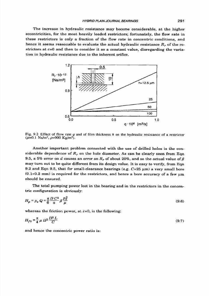
8/9/2019 Hydrostatic Lubrication 1992
http://slidepdf.com/reader/full/hydrostatic-lubrication-1992 308/558
HYBRID
PLAINJOURNAL BEARINGS
291
The increase in hydraulic resistance may become considerable, a t the higher
eccentricities, for the most heavily loaded restrictors; fortunately, the flow rate in
these restrictors
is
only a fraction
of
the flow rate in concentric conditions, and
hence it seems reasonable
t o
evaluate the actual hydraulic resistance
R,
of the re-
strictors at E=O and then to consider it as a constant value, disregarding the varia-
tion in hydraulic resistance due
to
the inherent orifice.
1.2
R, .I 0-12
[Ns/ms]
0.9
0.6
0.0 0.5 1 o
q 106 [rn3/s]
-rt , 0.5
.2
I
-
25
100
0.6'
'
I
0.0 0.5 1 o
q 106 [rn3/s]
Fig.
9.2
Effect of flow ate
q
and of film thickness h on the hydraulic resistance of a restrictor
(p=O.
1
Ns/m*, p 9 0 0 Kg/m3).
Another important problem connected with the use of drilled holes is the con-
siderable dependence of R, on the hole diameter. As can be clearly seen from Eqn
9.5, a 5% error on d causes an error on R, of about 20%, and so the actual value of B
may turn out t o be quite different from its design value. I t is easy t o verify, from Eqn
9.2 and Eqn
9.5,
that for small-clearance bearings (e.g. C=25pm) a very small bore
(0.1+0.2 mm) is required for the restrictors, and hence a bore accuracy of a few km
should be ensured.
The total pumping power lost in the bearing and in the restrictors i n the concen-
tric configuration is obviously:
x D C 3 P?
6 a
p =p s Q
=--B
whereas the friction power, at
E=O, is
the following:
(9.6)
(9.7)
and hence the concentric power ratio is:

8/9/2019 Hydrostatic Lubrication 1992
http://slidepdf.com/reader/full/hydrostatic-lubrication-1992 309/558
292 HYDROSTATIC
L
UBRlCATlON
(9.8)
When a load is applied, the journal is displaced, and, since
h
is no longer a con-
stant, an approximate solution
to
Eqn 9.1 has
t o
be looked
for.
For example, in ref.
9.1 a perturbation method is proposed in which a row of feeding holes is replaced by
a continuous band source. However, a more versatile way of solving this kind of
problem is by discretization methods, such as finite difference (ref. 9.2, 9.3) o r finite
element methods. Such methods prove
t o
be more accurate, especially a t high ec-
centricity, and can also take into account the effect of cavitation th at may set in a t
high velocities and eccentricities.
(i)
Load capacity .
The results obtained in ref. 9.2 for hybrid bearings a t P=0.5 are
summarized in Fig. 9.3, in which the non-dimensional load capacity
w'=- W
P S L D
(9.9)
is plotted, as a function of the eccentricity, for certain values of the geometric pa-
rameter
a
lL and of the power ratio Il (i.e. of the Sommerfeld hybrid number
Sh).
Figure 9.4 contains plots of the attitude angle
$.
Since the hydrodynamic effect is
a/L=O.l
/
0.1
I ,
W '
1 -
/'
/--,---I.-.---
0.25
_
0.0
0.5 1
o
&
Fig. 9.3 Load
W'
ersus eccentricity
E
(forJ=0.5 and
L / D = l )
or certain values of ratio
alL
and of
power ratio 9 ref. 9.2).
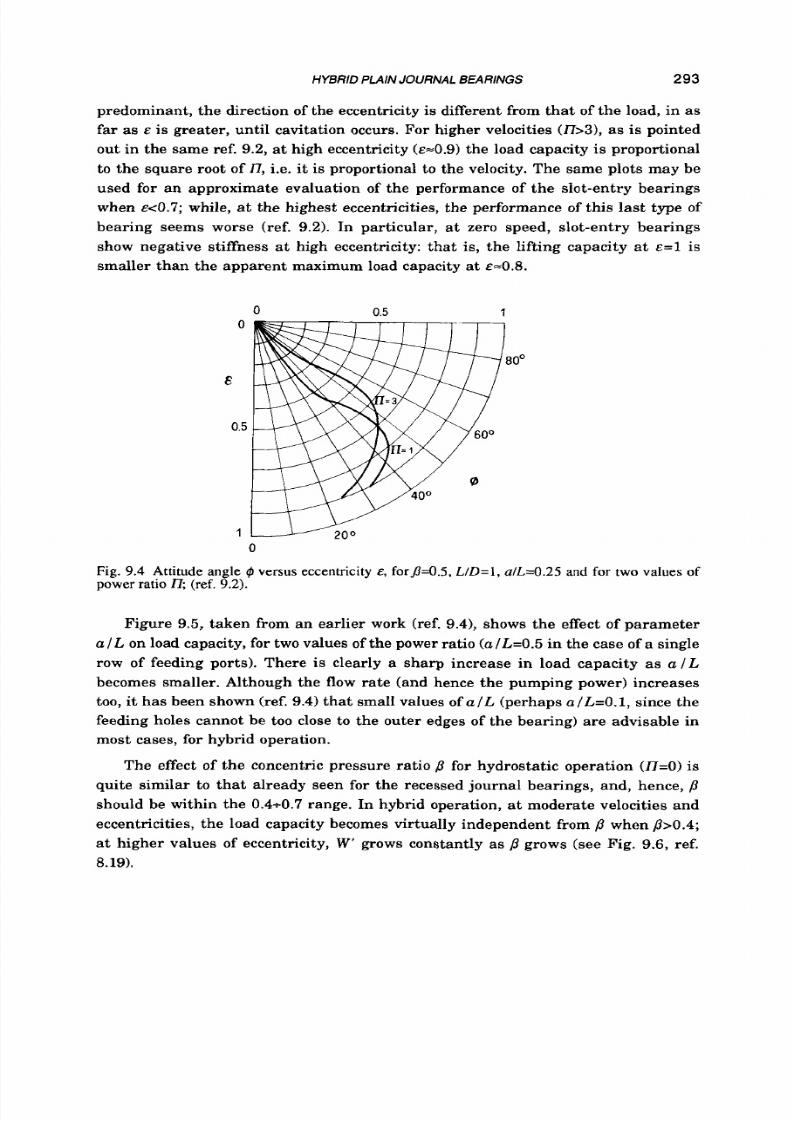
8/9/2019 Hydrostatic Lubrication 1992
http://slidepdf.com/reader/full/hydrostatic-lubrication-1992 310/558
HYBRID PLAIN JOURNAL B EARINGS
293
predominant, the direction of the eccentricity is different from that of the load, in as
far as
E
is greater, until cavitation occurs. For higher velocities
(17>3),
as is pointed
out in the same ref. 9.2, a t high eccentricity ( ~ ~ 0 . 9 )he load capacity is proportional
to
the square
root
of
Z7,
i.e.
it
is proportional to the velocity. The same plots may be
used for an approximate evaluation of the performance of the slot-entry bearings
when ~ 0 . 7 ;hile, a t the highest eccentricities, the performance of this las t type of
bearing seems worse (ref. 9.2). In particular, at zero speed, slot-entry bearings
show negative stiffness a t high eccentricity: that is, the lifting capacity
at
~ = ls
smaller than the apparent maximum load capacity at ~ ~ 0 . 8 .
0 0.5 1
0
Fig.
9.4
Attitude angle
4
versus eccentricity
E,
forfl=0.5,
L / D = l ,
alL=0.25
and
for two values of
power ratio
ZT
(ref.
9.2).
Figure
9.5,
taken from an earlier work (ref.
9.41,
shows the effect of parameter
a l L on load capacity, for two values of the power ratio
(a/L=0.5
n the case of
a
single
row
of feeding ports). There is clearly a sharp increase in load capacity as
a
1
L
becomes smaller. Although the flow rate (and hence the pumping power) increases
too,
it has been shown (ref. 9.4) that small values of a l L (perhaps
alL=0.1,
since the
feeding holes cannot be too close t o the outer edges of the bearing) are advisable in
most cases, for hybrid operation.
The effect of the concentric pressure ratio
,43
for hydrostatic operation
(n=O>s
quite similar
to
that already seen for the recessed journal bearings, and, hence,
p
should be within the 0.4+0.7 range. In hybrid operation, a t moderate velocities and
eccentricities, the load capacity becomes virtually independent from
/3
when /3>0.4;
at higher values of eccentricity, W'
grows
constantly as
f i
grows (see Fig. 9.6, ref.
8.19).
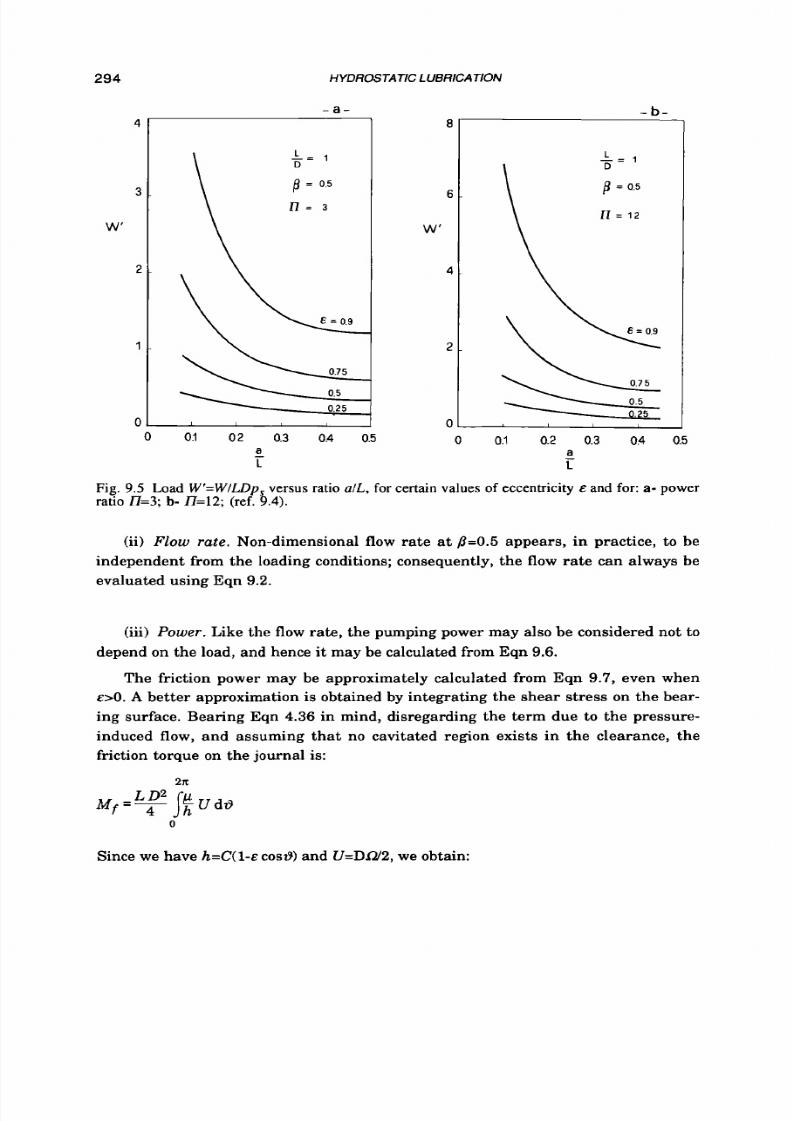
8/9/2019 Hydrostatic Lubrication 1992
http://slidepdf.com/reader/full/hydrostatic-lubrication-1992 311/558
294
4
3
W'
2
1
0
HYDROSTATIC LUBRICATION
- a -
- .
I
0
0.1
02 0.3
0.4 0.5
a
L
-
8
6
W'
4
2
0
I
0 0.1 0.2 0.3 0.4 0.5
a
L
-
Fig. 9.5 Load W'=WlLDp, versus ratio alL. for certain values of eccentricity E and for: a-
power
ratio
n=3;
-
II=12;
(ref.
9.4).
(ii)
Flow rate.
Non-dimensional flow rate a t p=0.5 appears, in practice, t o be
independent from the loading conditions; consequently, the flow rate can always be
evaluated using Eqn 9.2.
(iii)
Power.
Like the flow rate, the pumping power may also be considered not t o
depend on the load, and hence it may be calculated from Eqn
9.6.
The friction power may be approximately calculated from Eqn 9.7, even when
E>O.
A better approximation is obtained by integrating the shear stress on the bear-
ing surface. Bearing Eqn
4.36
in mind, disregarding the term due to the pressure-
induced flow, and assuming that no cavitated region exists in the clearance, the
friction torque on the journal is:
2a
Since we have
h = C ( l - ~
ostlt) and U = D N P ,we obtain:
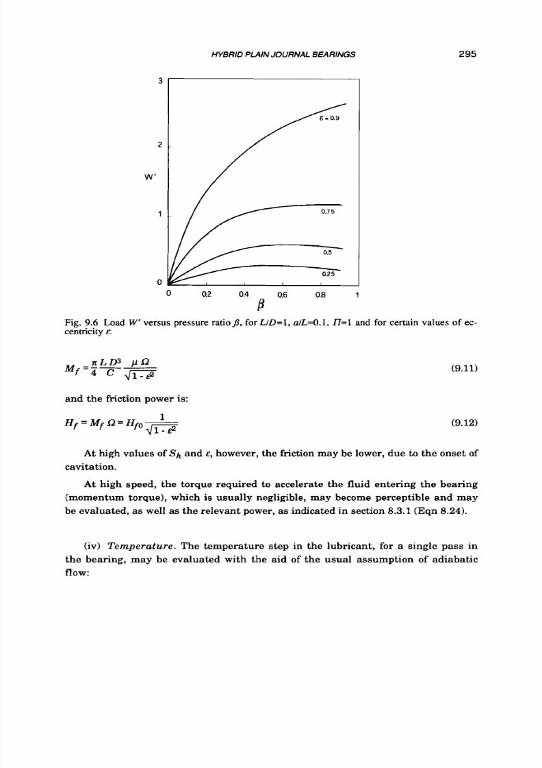
8/9/2019 Hydrostatic Lubrication 1992
http://slidepdf.com/reader/full/hydrostatic-lubrication-1992 312/558
W '
HYBRID PLAIN JOURNAL BEARINGS
-
~
-_
~ ~~~
3 1
0 0.2 0.4 0.6 0.8 1
B
295
Fig. 9.6 Load W' versus pressure
ratiofl, for
L / D = l , alL=O.l, I7=1 and for certain values
of
ec-
centricity E.
M n L D 3
f - 4 c
-
nd the friction power is:
1
H f = M f
0
Hi0
(9.11)
(9.12)
A t
high values of
s h
and
E,
however, the friction may be lower, due
t o
the onset
of
cavitation.
A t high speed, the torque required t o accelerate the fluid entering the bearing
(momentum torque), which is usually negligible, may become perceptible and may
be evaluated,
as
well
as
the relevant power, as indicated in section
8.3.1
(Eqn 8.24).
(iv)
Temperature .
The temperature step in the lubricant, for a single pass in
the bearing, may be evaluated with the aid of the usual assumption of adiabatic
flow:
8/9/2019 Hydrostatic Lubrication 1992
http://slidepdf.com/reader/full/hydrostatic-lubrication-1992 313/558
296
HYDROSTATIC LUBRlCATlON
(9.13)
It must be pointed out that careful control of lubricant temperature
is
more
important for the hybrid bearings than for the hydrostatic ones. If the temperature
rises, the consequent decrease in viscosity causes a considerable decrease in the
load capacity of the bearing (I7depends on the square of the viscosity). Hence it is
very important for the cooling system to be able
to
maintain viscosity below the value
used when designing.
9.3
DESIGN
OF
HYBRID BEARINGS
An optimization
of
a hybrid plain journal bearing may be based on the same
criteria already seen for the recessed bearings, i.e. mainly on the minimization of
the total power. Most of the remarks made in section
8.3.3
could, therefore, be re-
peated here, but there are certain differences, due to the fact that the hydrodynamic
effect plays an important role in sustaining the load. In particular, it is advisable
(ref. 9.4):
to use a small value for a / L e.g.a/L=O.l);
t o
allow greater eccentricities than for the recessed bearings b 0 . 6 ) ;
t o
select larger values for the concentric power ratio
(n>3).
Indeed, in the case of purely hydrostatic bearings the maximum eccentricity
must be limited because the stiffness is
very
poor when 00.6; in hybrid operation,
on the contrary, the load capacity increases sharply when
E
increases, and so stiff-
ness and overload capacity are ensured even when ~>0.9 . n the other hand, an
upper constraint to E may derive from other factors: e.g., at the higher eccentrici-
ties, a tilting error of the journal could cause the performance of the bearing
t o
dete-
riorate and even produce a localized contact.
The advisability
of
using higher values of the power ratio (as compared
t o
the
recessed hydrostatic bearings) is based on the fact that turning velocity not only
affects power expense, but also increases load capacity (this fact was disregarded in
the optimization of the hydrostatic bearings, section
8.3.3).
Consequently,
a 3<n<9
range is suggested for the power ratio (ref.
9.21,
although higher values could be
used.
The following is a possible procedure for the initial design of an hybrid bearing:
i) Select a set of geometrical parameters, with such typical values as
L / D = l ,
a
/L=O.l,
n=12
(this last parameter has little influence in hybrid operation,
provided
n>8).

8/9/2019 Hydrostatic Lubrication 1992
http://slidepdf.com/reader/full/hydrostatic-lubrication-1992 314/558
HYBRID PLAIN JOURNAL BEARINGS 297
ii) Select a suitable range for 8, and a maximum value for eccentricity, perhaps
0.4</3<0.7,and ~ ~ = 0 . 7 .igher values for
p
and
E
can be allowed in hybrid
operation, but not a t low velocities.
State
l7=3
and calculate the relevant
W'
coefficient from Fig. 9.3
or
Fig. 9.5.
Using Eqn 9.9, select the values of the diameter of the bearing and of feeding
pressure, keeping in mind that it is generally advantageous to have larger
bearings and lower pressures.
iii) Select a tolerance range 6, for the clearance (see Fig. 8.14). The maximum
and minimum values
C M
and C, are then calculated in such a way as to
ensure that p always remain in the proper range: e.g. if it has been stated
that 0.4<p<0.7, t must be
c m 2 0 . 6 6 - c ~
see also section 8.3.31, and hence
C ~ > 1 . 5 . 6 ~ ;
n the other hand, radial clearance should be small, since i t is
more suitable from the point
of
view of the power expense. The choice of the
tolerance range clearly follows from a reasonable compromise between
manufacturing and running costs. Furthermore, an upper constraint e M
may be required for the displacement e=&Cof the journal. In this case, if it
turns out that E&M>eM and Sg cannot be reduced, an attempt can be made
to select a smaller value for
EM
after which one must start again from point
(iii).
iv) From Eqn 9.8 calculate the optimal value of the viscosity:
If this value is impracticably great, and it is not possible to further reduce
C M , one may try to reduce
ps ,
increasing the bearing dimensions. If, on the
other hand, p is too small, one may choose t o increase the clearance, but it
might be more advisable to select a higher value for l7,and restar t the calcu-
lations from point (iii).
v) Calculate flow rate, pumping power and friction power.
Check the rise in temperature, using Eqn 9.13.
vi)
Design the compensating restrictors.
vii) Check the Reynolds number in the bearing clearance.
viii) Check the dynamic behavior of the system, especially as far as whirl insta-
bility is concerned (see Chapter 10).
If different loads have
to
be sustained at different velocities, the performance
of
the bearing should be checked in all the situations foreseen. In particular,
at
low
velocities (hydrostatic operation) stiffness is strongly reduced and, moreover, great
eccentricities
(&>0.6)
hould not be allowed.

8/9/2019 Hydrostatic Lubrication 1992
http://slidepdf.com/reader/full/hydrostatic-lubrication-1992 315/558
298 HYDROSTATIC L UBRICA TlON
9.4 CONCLUDING
REMARKS
Certain problems connected with hybrid bearings do not seem
t o
have been dealt
with yet in any depth. In particular, the isothermal flow model may be far from
representing the actual temperature profile in the clearance. Due to the great val-
ues of the power ratio needed
t o
get a high hydrodynamic load capacity, the temper-
ature step (Eqn 9.13) may prove to be considerable; furthermore, this is only an
average value, obtained by dividing the total power by the total flow rate . I t is easy t o
see that, actually, most
of
the lubricant flows directly outward (the entry ports are
close
to
the bearing edge) while the heat due to friction mainly develops in the lubri-
cant enclosed between the rows of supply ports, in the area of minimum clearance.
The temperature in this area is clearly much higher than the average value. Fur-
thermore, this hot lubricant, instead of being readily flushed out, may be recircu-
lated round the bearing, due
t o
the presence of the rows of entry ports (especially of
the slot type, that occupy practically the entire circumference with no interecess
land) and of large cavitated regions (ref. 9.5). Although other circumstances (heat
transport through the bearing sleeve, smaller friction power due to cavitation, back
flow
through the most heavily-loaded restrictors) may attenuate the temperature
peaks, it is clear t ha t bearing performance may be considerably affected.
Other problems involving the hybrid bearings may be (ref. 9.5) the existence
of
large cavitated regions (which may cause severe starvation problems), back flow
through the restrictors in the high pressure area (which occurs at high speed and
eccentricity, and thwarts the build up of the hydrodynamic pressure profile) and the
possibility of whirl instability. Instability is connected with the existence of a hydro-
dynamic side thrus t on the journal, revealed by the att itude angle (Fig. 9.4). In this
sense, cavitation may be considered beneficial and, hence, eccentricities larger than
&=0.6
hould be selected for hybrid operation.
Lastly, a peculiar type of hybrid bearing exists, characterized by the asymmetri-
cal configuration of its entry ports (ref. 9.5). Namely, each row is made up of a few
slots clustered symmetrically a t the bottom dead center, while a t the top dead center
there is an axial groove supplied a t low pressure (Fig. 9.7.b). This bearing presents
certain advantages, as compared with a usual slot-entry hybrid bearing (Fig. 9.7.a),
such as higher load capacity at small eccentricity, reduced cavitated regions,
smaller flow ra te and easily flushed-out hot fluid. On the other hand, a t high eccen-
tricity, load capacity is smaller, and (a t low speed) great negative stiffness occurs.
A
similar bearing (Fig. 9.8) is described in ref. 9.6 a s an alternative
to
conven-
tional generator bearings. The latter usually have small high-pressure pockets to
provide hydrostatic lift during start-up and shut-down operations, whereas in the
case of the hybrid bearing two rows of slot-type entry ports are also pressurized

8/9/2019 Hydrostatic Lubrication 1992
http://slidepdf.com/reader/full/hydrostatic-lubrication-1992 316/558
HYBRID PLAIN
JOURNAL BEARINGS 299
0
3
2
W
LDPS
1
0
a=I
I
I
I
- a -
*
n=9
a2
04 0.6 aa
I
&
-
b -
Fig.
9.7
Load versus eccentricity for a hybrid journal bearing with:
a-
twelve symmetrical slots per
row;
b-
fiv e slots per row and
an
axial groove.
[a=a,dRD is
the slot width ratio].
during normal running. The load support arc is
120
degrees wide and i s bounded by
large low-pressure inlet recesses. This type
of
hybrid bearing is claimed to be more
efficient than conventional generator bearings.
I
---
I
O I
l o
I ---
I
1
Fig. 9 .8 Slot-entry generator bearing.
8/9/2019 Hydrostatic Lubrication 1992
http://slidepdf.com/reader/full/hydrostatic-lubrication-1992 317/558
300
REFERENCES
HYDROSTATIC LUBRICATION
9.1
9.2
9.3
9.4
9.5
9.6
Ichikawa A.;
A
study of High Speed Hydrostatic Bearings (Part 1, Theoretical
Ana lysis of Static and Dynam ic Characteristics of Hybrid Pl ain Journ al Bear-
ings; Bull. JSME, 20 (19771,652-660.
Rowe W. B., Xu S. X., Chong F.
S.,
Weston
W.; Hybrid Journal Bearings;
Tribology Int., 15 (19821,339-348.
El Kayar A., Salem E. A., Khalil M. F., Hegazy A. A.; Two-Dimensional Fi-
nite Difference Solution for Externally Pressurized Journa l Bearings o f Finite
Length; Wear,
84
(1983),1-13.
Rowe W. B., Koshal D.; A New Basis for the O ptimization of Hybrid Journal
Bearings; Wear, 64 (1980), 115-131.
Ives D., Rowe W. B.; The E f fect of Multiple Supply Sources on the Perfor-
mance
of
Heauily Loaded Pressurized High-speed Journal Bearings;
Proc.
Inst. Mech. Engrs., C199 (19871, 121-127.
Ives
D.,
Weston W., Morton P. G . , Rowe W. B.;
A Theoretical Znuestigation of
Hybrid Jou rna l Bearings Applied to H igh-s pee d Heauily Loaded Conditions
Requiring Jacking Capabil i t ies;
Tribological Design o f Machine Elements,
proc. 15th Leeds-Lyon Symp. on Tribology, Leeds, 1988; p. 425-433.

8/9/2019 Hydrostatic Lubrication 1992
http://slidepdf.com/reader/full/hydrostatic-lubrication-1992 318/558
Chapter 10
DYNAMICS
10.1 INTRODUCTION
In previous chapters we have examined the behaviour of hydrostatic bearings
loaded by static forces. We now intend to evaluate the bearing response to time-
dependent loads; this means:
studying bearing stability; i.e. is the bearing able to return to its previous
equilibrium when excited by a small perturbation?
assessing bearing behaviour under given loads (impulsive and periodical, in
particular1.
A s a first step, the lubricant film may be assimilated to a mechanical system
formed by a (nonlinear) spring and
a
viscous damper, whose coefficient depends (in
a nonlinear way) on film thickness (Fig. 1O.l.a). Stiffness and damping can easily
be evaluated, without taking inertia and the compressibility of the lubricant into
account. On such assumptions, hydrostatic bearings always prove to be stable, but
in practice instability can sometimes arise. Actually, the compressibility of the oil
volume contained in bearing recesses and supply pipes and the compliance of the
tubing itself can play an important part in lowering the dynamic stiffness of bear-
ings and in causing instability. Moreover,
it
has
to
be borne in mind that, in practi-
cal cases, lubricant compressibility may be greatly increased by aeration phenom-
ena. Finally, the influence of the dynamic behaviour of the supply system (e.g. con-
trolled valves) must also be considered.
For a better approach
t o
bearing dynamics, more elaborate mechanical models
are often used (ref. 10.1, 10.21, like the ones in Fig. 10.l.b and Fig. lO.l.c, which
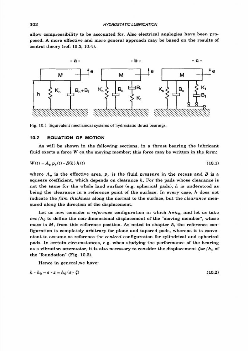
8/9/2019 Hydrostatic Lubrication 1992
http://slidepdf.com/reader/full/hydrostatic-lubrication-1992 319/558
302 HYDROSTATIC LUBRICATlON
allow compressibility to be accounted for. Also electrical analogies have been pro-
posed. A more effective and more general approach may be based on the results of
control theory (ref. 10.3, 10.4).
Fig. 10.1 Equivalent mechanical systems
of
hydrostatic thrust bearings.
10.2 EQUATION
OF
MOTION
As will be shown in the following sections, in a thrust bearing the lubricant
fluid exerts a force W on the moving member; this force may be written in the form:
where A,
is
the effective area, p r is the fluid pressure in the recess and
B
is a
squeeze coefficient, which depends on clearance
h. For
the pads whose clearance is
not the same for the whole land surface (e.g. spherical pads),
h is
understood as
being the clearance in a reference point of the surface. In every case,
h
does not
indicate the
fiam thickness
along the normal to the surface, but the
clearance
mea-
sured along the direction of the displacement.
Let us now consider a reference configuration in which
h=ho,
and let us take
E=e
1ho
to define the non-dimensional displacement of the "moving member", whose
mass is
M,
rom this reference position. As noted in chapter 5, the reference con-
figuration is completely arbitrary for plane and tapered pads, whereas it
is
conve-
nient to assume as reference the
centred
configuration for cylindrical and spherical
pads. In certain circumstances, e.g. when studying the performance of the bearing
as a vibration attenuator, it is also necessary to consider the displacement <=z / ho of
the "foundation" (Fig. 10.2).
Hence in genera1,we have:
h - ho
= e
z
=
ho E -
0 (10.2)
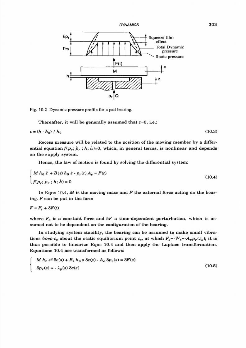
8/9/2019 Hydrostatic Lubrication 1992
http://slidepdf.com/reader/full/hydrostatic-lubrication-1992 320/558
DYNAMICS
303
Prs
1
Fig. 10.2 Dy n am ic pressure profile for a pad bearing.
Thereafter,
it
will be generally assumed that
z=O,
i.e.:
Recess pressure will be related t o the position of the moving member by a differ-
ential equation f ( p r ; , ;
h;
h)=O,which, in general terms, is nonlinear and depends
on the supply system.
Hence, the law of motion is found by solving the differential system:
(10.4)
In Eqns 10.4,M is the moving mass and F the external force acting on the bear-
ing. F can be put in the form
F
=
F,
+
6F ( t )
where F, is a constant force and 6F a time-dependent perturbation, which is as-
sumed not to be dependent on the configuration
of
the bearing.
In studying system stability, the bearing can be assumed to make small vibra-
tions
~ E = E - E ,
about the static equilibrium point E,, at which F , =- W , =- A , ~ , ( E , ) ;t is
thus possible to linearize Eqns 10.4 and then apply the Laplace transformation.
Equations 10.4 are transformed as follows:
(10.5)
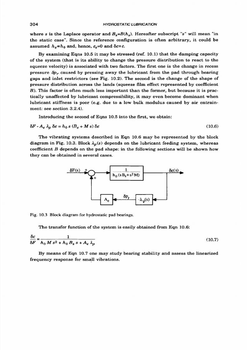
8/9/2019 Hydrostatic Lubrication 1992
http://slidepdf.com/reader/full/hydrostatic-lubrication-1992 321/558
304
HYDROSTATIC LUBRICATION
where s is the Laplace operator and B,=B(hL,).Hereafter subscript S will mean "in
the static case". Since the reference configuration is often arbitrary, it could be
assumed hs=hO and, hence, E,=O and
~ E = E .
By examining Eqns
10.5 it
may be stressed (ref. 10.1) that the damping capacity
of the system (that is its ability to change the pressure distribution to react to the
squeeze velocity) is associated with two factors. The first one is the change in recess
pressure
6p,
caused by pressing away the lubricant from the pad through bearing
gaps and inlet restrictors (see Fig. 10.2). The second is the change
of
the shape
of
pressure distribution across the lands (squeeze film effect represented by coefficient
B ) . This factor is often much less important than the former, but because it is prac-
tically unaffected by lubricant compressibility, it may even become dominant when
lubricant stiffness
is
poor
(e.g. due
t o
a low bulk modulus caused by air entrain-
ment: see section 3.2.4).
Introducing the second
of
Eqns 10.5 into the first, we obtain:
W -Ae jlp 6E
=
ho
s
(B , + M S)8~ (10.6)
The vibrating systems described in Eqn 10.6 may be represented by the block
diagram in Fig. 10.3. Block &(s) depends on the lubricant feeding system, whereas
coefficient
B
depends on the pad shape: in the following sections will be shown how
they can be obtained in several cases.
Fig. 10.3 Block diagram for hydrostatic pad bearings.
The transfer function of the system is easily obtained from Eqn 10.6:
8 E 1
W
-=
h ,
M
~2
+
ho B ,
s +Ae;lp
(10.7)
By means of Eqn 10.7 one may study bearing stability and assess the linearized
frequency response for small vibrations.

8/9/2019 Hydrostatic Lubrication 1992
http://slidepdf.com/reader/full/hydrostatic-lubrication-1992 322/558
DYNAMICS
305
10.3 PAD
COEFFICIENTS
The aim of this section
is
ta show how Eqn 10.1 may be written for a pad bearing.
In particular, the value of squeeze coefficientB must be calculated.
10.3.1
Circular-recess pads
Let us star t with the plane circular pad (Fig. 5.1.a) whose static behaviour has
already been examined in section 4.7.5 and section 5.3.
As
usual, we can start from
the Reynolds equation, in
this
case Eqn 4.23 which, assuming that film thickness is
uniform, becomes:
The above equation may be integrated twice to obtain the pressure pattern as
a
func-
tion of the boundary pressures, as well as of the angular and squeeze velocities L2
and
h:
The pressure
at
a certain radius proves to depend on the boundary pressures,
on the square of the rotation speed and on the squeeze rate in
a
linear fashion; this
will be true for every shape of pad, since it is
a
consequence of the linearity of the
Reynolds equation. The load capacity of the pad may therefore be calculated (as in
Eqn 10.1) by adding the term A,p,, already known from chapter
5,
o the term
Wd=-Bh obtained by integrating the following squeeze overpressure on the land
surface:
The followingis
easily
found
(10.8)
CoefficientB is plotted in Fig. 10.4.a, in which it must obviously be taken that
a=d2.
Another parameter related
t o
the squeeze effect, that will prove to be useful in
the following section, may be introduced a t this point; it is defined by the following
equation:
(10.9)
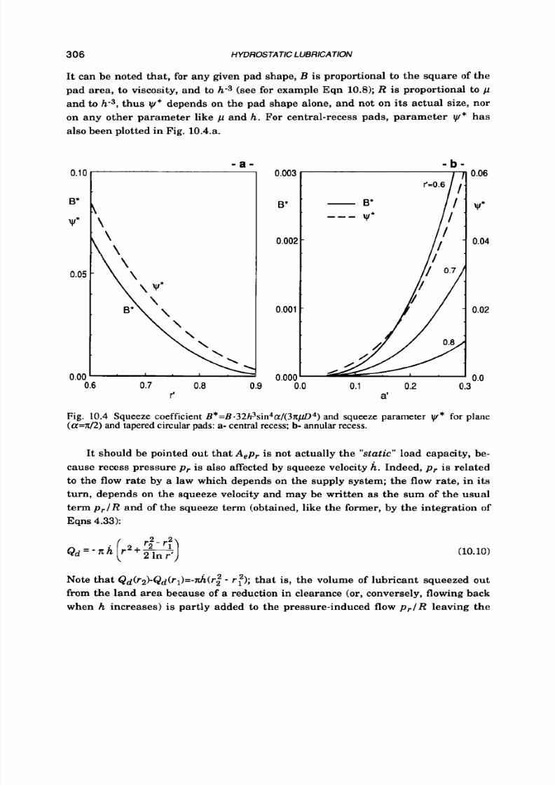
8/9/2019 Hydrostatic Lubrication 1992
http://slidepdf.com/reader/full/hydrostatic-lubrication-1992 323/558
306
HYDROSTATIC LUBRICATION
It can be noted that, for any given pad shape,
B
is proportional
t o
the square of the
pad area, t o viscosity, and t o
h-3
(see for example Eqn 10.8);R
is
proportional to p
and to
h-3 ,
hus ay * depends on the pad shape alone, and not on its actual size, nor
on any other parameter like
p
and
h .
For central-recess pads, parameter
a y *
has
also been plotted in Fig. 10.4.a.
- a - - b -
r'
a'
Fig.
10.4
Squeeze coefficient
B* = B
.32h3sin4a/(3qfD4)and squeeze parameter
a y *
for plane
( a = x / 2 ) and tapered circular pads:
a-
central recess:
b-
annular recess.
It should be pointed out that
A,pr is
not actually the
"static"
load capacity, be-
cause recess pressure
p r
is also affected
by
squeeze velocity
h.
Indeed,
p r
is related
to the flow rate by a law which depends on the supply system; the flow rate, in its
turn, depends on the squeeze velocity and may be written as the sum of the usual
term p r IR
and of the squeeze term (obtained, like the former, by the integration
of
Eqns 4.33):
(10.10)
Note that Q d ( r 2 ) - Q d ( r l ) = - & ( r ~
r : ) ;
that is, the volume of lubricant squeezed gut
from the land area because of a reduction in clearance
(or ,
conversely, flowing back
when
h
increases) is partly added to the pressure-induced flow p r I R leaving the
8/9/2019 Hydrostatic Lubrication 1992
http://slidepdf.com/reader/full/hydrostatic-lubrication-1992 324/558
DYNAMICS 307
outer boundary of the land, and partly subtracted from the same flow p , l R entering
at th e inner boundary. In particular, it may be easy to see that the flow rate crossing
the recess boundary (i.e. a t radius
r = r l )
is:
where A, is the projected area of the recess (in this case, simply Ar=zr;) and A, is
the effective bearing area of the pad, viz. the ratio of the static load capacity to the
recess pressure.
Equation 10.11 may be considered to be of general validity, whatever the shape of
the pad.
10.3.2 Annular-recess pads
recess pads of the type shown in Fig. 5.13:
Proceeding a s above, the squeeze coefficient is easily obtained for the annular-
I
(10.12)
A plot of
B
and w* (Eqn 10.9) is given in Fig. 10.4.b, both for tapered and flat (a=x/2)
annular-recess bearings.
10.3.3 Tapered pads
For the pads in Fig. 5.19, we may assume that h=h,lsina, where h, is the film
thickness over the land surface. The following
is
easily obtained (see ref. 10.5) for
a
central recess pad:
(10.13)
that is, it equals the coefficient
B
already obtained for the flat pad (Eqn 10.81, divided
by sin4a. Equation 10.13 is plotted in Fig. 10.4.a.
Coefficient B for the annular-recess pad may be obtained in the same fashion,
namely by dividing Eqn 10.12 by sin44 and
it
may be found in Fig. 10.4.b.
8/9/2019 Hydrostatic Lubrication 1992
http://slidepdf.com/reader/full/hydrostatic-lubrication-1992 325/558
308 HYDROSTATIC LUBRlCATlON
10.3.4
Screw and nut assemblies
Equation 10.13 and Fig. 10.4may also be used for the hydrostatic screw and nut
assemblies (see Fig. 5.35), substi tuting sina with cose, i.e, with the cosine of the
flank angle. If hydrostatic lubrication is extended over more than one turn of the
screw,
B
must also be multiplied by n (the number of active turns).
10.3.5 Other pad shapes
In general, the Reynolds equation cannot be explicitly integrated, for a generic
pad shape, and approximate solutions should be looked for.
For
the sake of clarity,
let
us
consider a plane pad of any shape; the relevant Reynolds equation will be
(from Eqn
4.15):
a a a a
zh3 Z P )
+ ( h 3
Z P ) =
12P h
(10.14)
to which the inner and outer boundary conditions p = p r on
ri
and
p=O
on
ro
have to
be added. If the film thickness h is not uniform (e.g. tilted pads), another term
should be added, depending on the bearing velocities in directions
x
and z .
Since Eqn
10.14 s
linear, the differential problem can be split into two parts:
$(ha ,PO)+
g h3
P O )
=0
;
p O = p r
on
;
p O = O on
To
(10.15)
(10.16)
where
P'Pa+Pd is
the solution being sought.
It
is
easy to see that p a is the static pressure distribution for the given boundary
conditions, while P d is the dynamic overpressure due to the squeeze effect. If tan-
gential velocities have to be accounted for, another term
p u
could be evaluated in the
same way. Similar considerations hold good for pads of any shape, cylindrical,
spherical, and
so
on.
The solution of the static problem (Eqns
10.15)
as been dealt with in Chapter
5 ,
leading to the evaluation of the effective area A,, and Eqns
10.16
may be solved with
the aid of the same numerical methods. Whatever the method (for instance finite
differences, finite elements, as well as boundary elements), a pressure distribution
pd,
proportional
to
the squeeze
rate h ,
will be obtained. If we integrate the pressure
Pd on the whole land area, we may evaluate the contribution
Sh
of squeezing to the
load capacity of the land itself, which has
to
be added to the static load capacity and,
if necessary, to a hydrodynamic term depending on tangential velocity.
8/9/2019 Hydrostatic Lubrication 1992
http://slidepdf.com/reader/full/hydrostatic-lubrication-1992 326/558
DYNAMICS 309
In many cases, however, coefficients B and
ty*
may be totally disregarded.
Indeed, it will be shown in section
10.5
hat, when the compressibility of the lubri-
cant
is
negligible, the damping of the bearing is little affected assuming
B=O.
On the
contrary, when the lubricant stiffness
is
poor, as compared to the bearing stiffness,
the squeeze film effect may become important in assessing bearing stability. How-
ever, B may be evaluated roughly by dividing the land area into parts with simple
shapes, whose contribution to squeeze may be easily obtained.
For
instance, the land
of a rectangular pad may be split up in the way shown in Fig. 5.26; or parts 1 o 4
the expression of the squeeze load of an indefinite rectangle can be used:
while each corner can be approximated by an arc
of
a circular ring, for which
The flow rate can be found
for
a given pressure distribution by integrating the
flow vector q,
whose components are given in Eqns
4.32:
Q = q v dT
r
where
I- is
a closed contour of which v
is
the normal external direction. Again, the
flow rate will be the sum of the static and dynamic terms. If Tis the inner contour
of
land area, the result will be an equation such as Eqn
10.11.
10.4 SUPPLY
SYSTEMS
In order to write the second of Eqns 10.4,we may state the continuity between
the flow rate
Q
delivered by the supply system and the flow rate entering the
bearing.
With reference to Fig.
10.5,
he difference between flow rate Q and flow rate Qi
entering the bearing clearance is equal to the volume variation of the recess and
relevant tubing, to which the effect of the lubricant density variation hasto be added:
(10.17)
P
Qi Q
=
- V
-
-
The total volume
V
is the sum of recess volume
V,.
and of tubing volume
Vt;
hence:

8/9/2019 Hydrostatic Lubrication 1992
http://slidepdf.com/reader/full/hydrostatic-lubrication-1992 327/558
31
0
HYDROSTATIC LUBRICATION
Fig. 10.5 Flow rates in a pad bearing: Q flow rate delivered by the supply system; Qi f low rate
entering the bearing clearance (in static conditionsQ=Qi).
av, .
V =
V,.
+ V, = A ,
h
+
-pr
apr
(10.18)
(here we assume that pressure
p ,
is uniform in the recess and pipes up to the com-
pensation devices); A, is the projected area of the recess. The term
aV,lap,
is due to
tubing compliance and, in general, may be regarded as a constant. Density p may
be considered
to
depend solely on pressure, hence
where Kla is the apparent bulk modulus of the lubricant (see section 3.2.4).
Let us now define the lubricant stiffness
Kd
as:
Bearing in mind Eqn 10.11, Eqn 10.17 becomes:
(10.19)
(10.20)
From the point of view of flow continuity, the bearing may be represented by the
hydraulic system in Fig. 10.6; Q is the volume
flow
rate delivered by the supply de-
vices,
R
is the hydraulic resistance of the bearing clearances. In dynamic condi-
tions, the flow rates of a spring accumulator (whose spring stiffness and section
area are Kd and A,, respectively) and of a piston (section area A,) fastened to the
moving member of the bearing have to be added to flow Q delivered by the supply
system.
It should be pointed out that a number of simplifications have been introduced
in developing the foregoing equations. In particular, we have assumed that the
pressure is uniform in the recess and in the ducts connecting the recess to the com-
pensation device (o r to the pump), that the compressibility of the lubricant in the

8/9/2019 Hydrostatic Lubrication 1992
http://slidepdf.com/reader/full/hydrostatic-lubrication-1992 328/558
DYNAMICS
31
1
Fig. 10.6 Equivalent hydraulic system of
a pad
bearing.
clearance may be disregarded (since the volume of lubricant in the clearances is
very small), and tha t the inertia of the lubricant is negligible. On the other hand, in
certain circumstances (such as long supply pipes and low viscosity), other dynamic
phenomena may occur, such as pressure waves in the supply pipes, that will not be
considered here.
In the following sections, several supply systems will be examined, for each of
which an expression of the flow rate Q will be found and introduced into Eqn 10.20.
The second of Eqns 10.4 will thus be obtained and then linearized in order to write
an equation for block
A,
which appears in the block diagram (Fig.
10.3)
and in the
relevant transfer function (Eqn 10.7). n applying small perturbation linearization,
one should remember that, as a general rule, the hydraulic resistance of the bear-
ing is proportional to h-3 (a t least in the case of small amplitude vibrations), hence
(10.21)
is
the perturbation of
1lR.
10.4.1
Direct supply (constant
f low)
The supply system is constituted simply by
a
positive displacement pump,
which delivers a flow rate Q which is not dependent on recess pressure
pr.
There-
fore, the equivalent hydraulic system shown in Fig.
10.6
may be completed by substi-
tuting the "supply" block with a constant-flow pump.
Equations 10.4 can now be written in the form:
(10.22)

8/9/2019 Hydrostatic Lubrication 1992
http://slidepdf.com/reader/full/hydrostatic-lubrication-1992 329/558
31
2 HYDROSTATIC LUBRICATION
W,=-F,
is the static load capacity of the bearing in the position of equilibrium
es=O,
and R , the relevant hydraulic resistance of bearing clearances.
Equations 10.22 constitute a third order nonlinear system, which may be inte-
grated by numerical means or linearized (see also appendix A.2). Applying the
small perturbation method and the Laplace transformation, we obtain:
(10.23)
Bearing Eqn 10.21 in mind, and comparing Eqns 10.23 with Eqns 10.5, it is easy
to find the following expression of block
&:
The characteristic frequencies
w1
and w 2 take on the following values:
Kd
0 2 = A x ;
Ks
01=A2,R, ;
(10.24)
(10.25)
K, is the static bearing stiffness
(see Eqn
6.51,
and Kd is the lubricant stiffness. In this connection, in evaluating Kd
(by means of Eqn 10.191, it is important
to
take into account the volume of lubricant
contained not only in the recess but also in the entire length of the feeding pipes
back
to
the pump.
We can now resort to Eqn 10.6 governing the dynamic behaviour of the bearing
system in the case
of
small-amplitude vibrations; the relevant transfer function
(Eqn 10.7) will be examined in section 10.5 in order to assess stability and frequency
response.
10.4.2
Compensated supply (constant pressure)
The bearing
is
fed by a system which is able to maintain a constant pressure
p s
over a compensation device, whose hydraulic resistance may be constant (capillary
restrictor or similar devices) or depend on the pressure step (in most case orifices,
though elastic restrictors have also been proposed). The overall hydraulic scheme of
the bearing is, then, the one to be seen in Fig. 10.7.

8/9/2019 Hydrostatic Lubrication 1992
http://slidepdf.com/reader/full/hydrostatic-lubrication-1992 330/558
DYNAMICS
313
Fig.
10.7
Equivalent hydraulic system of a pad bearing supplied at constant pressure, compensated
by:
a-
a fixed restrictor;
b-
a
spool
valve; c- an infinite-stiffness valve.
The volume rate of flow passing through a laminar-flow restrictor
R ,
is easily
written (see Eqn 6 .19 )as:
whereas
for
an orifice we find (Eqn
6.24):
P s c E z p
& = Ro
(10.26)
(10.27)
As
usual,
p
is the pressure ratio
p r I p s
in the reference configuration
h=ho.
Equating the right-hand members
of
Eqn 10.20 and Eqn 10.26, the desired differ-
ential relation between
p ,
and E is obtained

8/9/2019 Hydrostatic Lubrication 1992
http://slidepdf.com/reader/full/hydrostatic-lubrication-1992 331/558
314
HYDROSTATIC
LUBRlCATlON
In order to study stability and low-amplitude frequency response, one may lin-
earize and then apply Laplace transformation, thus obtaining:
from which
it is
easy to find the transfer function of block $ in Fig.
10.3. A
similar
equation may clearly be obtained in the case of orifice restrictors:
In both cases Ap may just be written as in Eqn
10.24,
but the characteristic fiequen-
cies are now:
The value of parameter
0 s:
(capillary)
(orifice)
(10.28)
(10.29)
As usual, Kd indicates lubricant stiffness (Eqn
10.19),
while Ks
s
the static stiffness
of the bearing (Eqn
6.23
and Eqn
6.26)
that may
a l s o
be written in the following form:
(10.30)
10.4.3
Control led restr ictors (constant pressure)
The bearing
is
now fed by
a
constant pressure system through
a
compensation
device whose hydraulic resistance will depend on the degree of freedom of a moving
element (e.g. a membrane) which, in its turn, will depend on the pressure step and
sometimes on the rate
of
flow being supplied, too. The transfer function of the over-
all system will obviously depend on a larger number of time constants than in pre-
vious cases, since the parameters describing the dynamics of the valve have to be
accounted for. This section will show the way the dynamic study of such a device
may be planned; in the following sections a few particular kinds of valve will be ex-
amined in
a
little more detail.
In order to evaluate
A
for passively compensated systems, Eqn
10.20,
express-
ing inlet flow rate Q as a function of the recess pressure and the position of the bear-

8/9/2019 Hydrostatic Lubrication 1992
http://slidepdf.com/reader/full/hydrostatic-lubrication-1992 332/558
DYNAMICS
315
ing, has been put together with another equation expressing the rate of flow from
the supply system as a function ofp, (e.g. Eqn 10.26); the block ;lp was easily ob-
tained by eliminating Q and performing linearization. In the case of controlled
devices, the supply flow rate may be expressed as a function of
x
(the degree of free-
dom of the valve) and of its time derivative, as well as of p,:
Since another degree of freedom has been introduced in the system, another
equation is required, which can be obtained by writing down the balance of forces
acting on the moving member of the pressure-compensating device; in general, this
relation can be written as:
Substituting Eqn
10.20
for Q in both Eqn
10.31
and Eqn
10.32,
after performing
small perturbation linearization and Laplace transformation, the two equations
will take the following form:
(10.33)
The relevant block diagram in is shown in Fig. 10.8. Note that
Ap0
is the value
that the transfer function
;lp
would have for &=O (i.e. if the moving member of the
controlled valve was "blocked" a t it s static position); and
&&
must be null func-
tions when valve control is not sensitive to pressure or to flow rate (and hence to
E ) ,
respectively.
A n expression for block
is easily obtained from Eqns 10.33:
(10.34)
The bearing transfer function will, formally speaking, remain Eqn 10.7, pro-
vided the above value is substituted for %. In the following sections, we shall exam-
ine a few examples of controlled devices.
10.4.4
Spool or diaphragm
valves
The static behaviour of spool and diaphragm devices has already been dealt with
in chapter 6: in both cases the moving member reaches
a
position of balance due to
the opposing thrusts of an elastic element and recess pressure pr. The hydraulic
resistance of the valve therefore depends on the degree
of
freedom (namely
" x " ) of

8/9/2019 Hydrostatic Lubrication 1992
http://slidepdf.com/reader/full/hydrostatic-lubrication-1992 333/558
31
6
HYDROSTATIC LUBRICATION
Eo,
Fig. 10.8 Block diagram for a hydrostatic pad bearing compensated by means of a controlled valve.
the device, with a law R,=R,(x), which, in general cases,
is
a non-linear one. If the
valve restrictor
is
not laminar, a more complicated law R,=R,(x,
pr )
will emerge.
As indicated above, the flow rate delivered by the valve in dynamic conditions
must be written as a function of x and p,.. From Fig. 10.7.b it follows that Q is the
sum of the flow rate passing through the variable hydraulic resistance R , and of the
volume of lubricant displaced by the moving spool:
Q
=-Ps
- Pr + A, x
Rr
(10.35)
Note that , in the case of the diaphragm valve, x will be the displacement of the cen-
tre of the membrane and A, will be an "effective" area. Substituting Eqn 10.20 or
Q,
Eqn 10.35 becomes:
(10.36)
Equation 10.32 is,
in
this case:
M , X + K , X + A , ~ , = F , ~
(10.37)
where M u ,
K ,
and
A,
are the spool mass, the spring stiffness and the spool section
area, respectively; is a constant (namely, the spring force for x=O) .
The set of differential equations made up by Eqn 10.36, Eqn 10.37 and the first of
Eqns 10.4 describes the dynamic behaviour of the bearing system.
As
usual, in the
case of small amplitude vibrations, linearization may be carried out. For the sake of
simplicity, let us limit ourselves to examine the case
of
small vibrations around the
8/9/2019 Hydrostatic Lubrication 1992
http://slidepdf.com/reader/full/hydrostatic-lubrication-1992 334/558
DYNAMICS 317
reference configuration
h,=ho
(hence, E,=O and B E = ) . In the neighbourhood of
E=O,
R,
may be written as:
R,
=
R,,
+
m,
=
+
C,
6e
+ c u p
p ,
(10.38)
P
The coefficients
C,
and
C u p
should be evaluated by considering the constructive
details of the device. If R, is a laminar-flow restrictor, i t is simply C,=O; whereas,
if the restrictor is a true orifice, it is
1 Ro
C u p = - @ p,
For the devices considered in sections 6.3.4 and 6.3.5, coefficientC,may be writ-
ten as
c,=---
Ku
Ro
P” A , Ps
The reader may refer to the relevant sections for the meaning of the symbols used
above. It is easy
to
see that the complex operators which appear in Eqns 10.33, and
hence in Eqn 10.34, are in this case the following:
(10.39)
In the equations above, KO,is the static stiffness of the bearing supplied through a
fixed restrictor Rr=RrOwith the same pressure ratio
P :
w, 1
ho
0
K w = 3 - -
Coefficient
CT
is given by
(10.40)
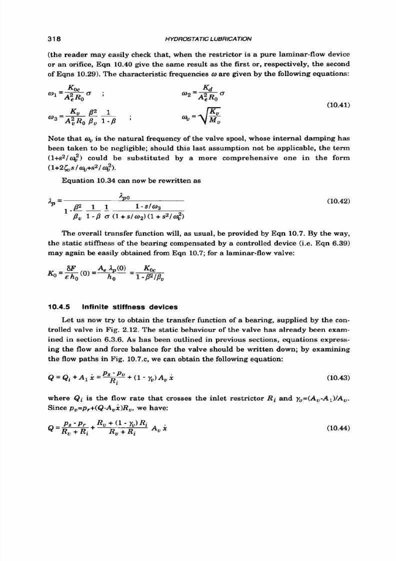
8/9/2019 Hydrostatic Lubrication 1992
http://slidepdf.com/reader/full/hydrostatic-lubrication-1992 335/558
318
HYDROSTATIC LUBRICATlON
(the reader may easily check that, when the restrictor is a pure laminar-flow device
or an orifice, Eqn
10.40
give the same result as the
first or ,
respectively, the second
of Eqns 10.29).The characteristic frequencies o re given by the following equations:
(10.41)
Note that q, s the natural frequency of the valve spool, whose internal damping has
been taken to be negligible; should this last assumption not be applicable, the term
(l+s2/a$) could be substituted by a more comprehensive one in the form
(1+2CVS
%+S2/
o&.
Equation
10.34
can now be rewritten as
(10.42)
The overall transfer function will, as usual, be provided by Eqn 10.7. By the way,
the static stiffness of the bearing compensated by a controlled device (i.e. Eqn 6.39)
may again be easily obtained from Eqn
10.7;
for a laminar-flow valve:
10.4.5
Infinite stiffness devices
Let us now try to obtain the transfer function of a bearing, supplied by the con-
trolled valve in Fig. 2.12. The static behaviour of the valve has already been exam-
ined in section 6.3.6.
As
has been outlined in previous sections, equations express-
ing the flow and force balance for the valve should be written down; by examining
the
flow
paths in Fig. 10.7.c, we can obtain the following equation:
(10.43)
where Q i is the flow rate that crosses the inlet restrictor R i and y,=(Av-A,)lAv.
Since pU=pr+(Q-AvX)Rv , e have:
(10.44)

8/9/2019 Hydrostatic Lubrication 1992
http://slidepdf.com/reader/full/hydrostatic-lubrication-1992 336/558
DYNAMICS
319
Force balance on the spool gives:
M , X + A , P ~ - ~ ~ ~ - A ~ ~ ~ , = O (10.45)
and hence
The laminar restrictor
Rd,
which has no effect on static behaviour, may be added to
increase the damping of the movements
of
the spool.
As
usual, the compressibility
of the lubricant in the device has been disregarded.
The hydraulic resistance
Ri
is, in general, dependent on the position of the spool
and on pressure p u .For small-amplitude vibrations
it
may be stated, that
Of course, it would be C=O
for
plain laminar flow: for the sake of simplicity, let us
limit to this las t case.
Eliminating Q from Eqn 10.44 and Eqn 10.46 by means of Eqn 10.20, two differen-
tial equations in E, x and p r are obtained, which, added
to
the first of Eqns 10.4, allow
the problem to be solved numerically. For small vibrations around the reference
configuration E=O, by linearizing and Laplace-transforming, a set of equations like
Eqns 10.33 is obtained. After a number of manipulations, the following equations
may be written:
s
1 + -
1 + -
" 2
1- -
Kocho 1
& 0 = 7
-
S
PSCV " 3
;1 =p2--
s
Ro
1 + -
A? 1 -
;1 =- 1 Kocho 1 0 1
Rd
s
1 + -
"2
& P = - A X Rd 1 + -
l+-
Y V R V @4
s
1 + -
V& l - p A v A e R o
l . + -u Rv
(
i4
(10.47)

8/9/2019 Hydrostatic Lubrication 1992
http://slidepdf.com/reader/full/hydrostatic-lubrication-1992 337/558
320 HYDROSTATl C LUBRICATION
A s
before, Koc and A are, respectively, the static stiffness and the value of
A,
for
Cv=O that is, the values th at would be obtained if the spool was blocked). We have
stated
10.5 DYNAMICS OF SINGLE-PAD BEARINGS
10.5.1 Transfer function
The block diagram representing the dynamics of a thrust bearing has been
presented in section 10.2 (Fig. 10.3), as well as the relevant transfer function (Eqn
10.7). The block A which appears in Eqn 10.7 stands for the feedback of the system:
namely it shows how the system reacts, dynamically changing the recess pressure,
to displacements induced by load variations.
In section 10.4 it has been shown how $ depends on the lubricant supply system
and on the lubricant itself (namely, on its compressibility). In particular, in the
case of passive compensation (e.g. a constant flow pump or fixed restrictors)
Ap
is
given by Eqn 10.24. The characteristic frequencies o1 nd
02,
on which mostly
depends the dynamic behaviour of the system, turn out to be proportional to bearing
stiffness
K ,
and to lubricant stiffness
Kd,
respectively (of course l / w 2 = 0 when com-
pressibility
is
negligible); they may generally be written in the form of Eqn 10.28, in
which the value of constant
Q
depends on the type of supply system (namely, we
have to take o=l in the case of direct supply by a constant-flow pump, or a value
calculated by means of Eqns 10.29 for capillary and orifice compensation).
In the case of an "active" supply system (e.g. constant flow valves
or
"infinite
stiffness" devices) block
$
s obviously more complicated (see a l s o ref. 10.4 and 10.6):
recess pressure
p,.,
in fact, depends also on another variable
x
(the degree
of
free-
dom of the supply device), which, in turn, depends on recess pressure and some-
times on the hydraulic resistance of the bearing, and hence on E . This argument
has been treated in sections 10.4.3 to 10.4.5.
In the case of passive compensation it may be interesting
to
return to the equiva-
lent mechanical system of Fig. 10.l.b, and search the values to be assigned
to
opera-
tors K 1 and
B , .
We can write the linear differential equations which describe the
mechanical system and then obtain the relevant transfer function; having estab-
lished tha t it must be identical to Eqn 10.7,it turns out that:

8/9/2019 Hydrostatic Lubrication 1992
http://slidepdf.com/reader/full/hydrostatic-lubrication-1992 338/558
32
(10.49)
It
is
obvious that K, and B, turn out to be negative when &<K8 and, conse-
quently, the system may prove to be unstable. On the contrary, when fluid com-
pressibility
is
very
poor
(that is Kd>>K8),
Kl
an be substituted by
a
rigid connection
and the model in Fig. 10.l.b
is
reduced to the second order model in Fig. 10.l.a,
where the spring stiffness
is
K=K,, and the damping constant
is
B,+K8101. Thus, in
the case of
a
passive supply system and negligible fluid compressibility, Eqn 10.7
takes on the usual appearance of the transfer function of second order vibrating
systems:
(10.50)
where
wn
nd ( are, respectively, the undamped natural frequency and the damp-
ing factor of the system:
(10.51)
Parameter
t , ~
s defined, beai -.ig a
ing equation:
,o
in mind Eqn 10.9 and Eqns 10.28,-y the follow-
(10.52)
Since
w*
s, in general, much smaller than unity, the squeeze film effect may be
disregarded when evaluating the damping factor in the case of incompressible lu-
bricant. If we want to include compressibility, Eqn 10.50 must be substituted by the
following transfer function
where

8/9/2019 Hydrostatic Lubrication 1992
http://slidepdf.com/reader/full/hydrostatic-lubrication-1992 339/558
322
HYDROSTATIC LUBRICATION
10.5.2 Stabi l i ty
In the previous section it has been shown that a single-effect passively compen-
sated bearing, making small amplitude vibrations, behaves in exactly the same way
as the mechanical system in Fig. 10.l.b)provided that condition
Kd>Ks
is satisfied;
that is , the stiffness of the lubricant in the recess and relevant tubing (and the stiff-
ness of the tubing itself ) must be greater than the static stiffness of the bearing.
This proves to be a sufficient condition
for
stability (the mechanical systems in Fig.
10.1
are always stable when spring and damping constants are greater than zero).
Condition Kd>K, is often easily satisfied due to the great bulk modulus of lubricants,
while in gas bearings stability is often an important factor
to
be dealt with. Problems
may, however, arise when:
- the recess and relevant tubing contain a large volume of lubricant;
-
rubber hoses ar e used to connect compensation devices to the recess;
-
the lubricant may hold a great amount of air.
This last factor is the most dangerous, because, in practical applications, it is
not easy
t o
forecast quantitatively the compressibility increase due to aeration.
A less restrictive condition for the stability of Eqn 10.53 may be obtained by
means of the well known Routh or Hurwitz criteria (ref.
10.7).
These methods con-
sists in checking if the coefficients of the characteristic equation of the system sat-
isfy o r not certain conditions. In our case, the characteristic equations is:
For a third-order system
to
be stable, the Routh criterion requires that all the coeffi-
cients ai of the characteristic equation, as well as the parameter
a3
a0
b = a , - -
a2
(10.55)
(each ai indicates the coefficient of the relevant power of
s
in the characteristic equa-
tion) must have the same sign. Since all the ai are greater than zero, the system
proves to be stable when:
(10.56)

8/9/2019 Hydrostatic Lubrication 1992
http://slidepdf.com/reader/full/hydrostatic-lubrication-1992 340/558
DYNAMICS 323
All the parameters in Eqn 10.56 are positive, and then the right-hand
side
is
always less than unity; this confirms that {>1 is a sufficient condition, tallying with
the limit case of
B=O.
On the other hand, if
B
and are great enough, the right-hand
side becomes negative and stability is clearly ensured whatever the value of
K d,
although the effective damping of the system may prove to be very poor, for low lu-
bricant stiffness, in spite of high values of
c.
Bearing in mind that ty depends on the shape of the bearing (see section 10.31,
it
may be concluded that , from the point of view
of
dynamic behaviour, i t is advisable
to design bearing with large lands in order t o increase the margin of stability when
the lubricant compressibility is not low enough
t o
ensure tha t Kd
is
safely greater
than K,.
When controlled devices are used for pressure compensation, Eqn 10.7 proves to
be of a higher degree and depends on a larger number of time constants. Instability
could now occur even when lubricant compressibility is negligible. For instance, let
us consider a diaphragm-controlled restrictor and assume that the mass of the
diaphragm is very low: in other words we assume that w, is much greater than
w 1
and w 3 , Equation 10.42 may, therefore, be simplified as follows:
(10.57)
We can now substitute Eqn 10.57 into Eqn 10.7, draw the characteristic equation
(which is again of degree 3) and examine
its
coefficients: i t is easy to see that the
coefficient of s2may become negative for certain values of@2/PU: clear symptom of
instability As before, a more detailed analysis of stability can be carried out by ap-
plying the Routh criterion t o the coefficients of the same characteristic equation.
Furthermore, for the sake of simplicity, we may disregard the squeeze coefficient
B,
and thus it is easy to see that instability is likely to occur when
(the last term on the right-hand side does not actually depend on But as shown by
Eqn 10.41). It is interesting t o note that often ~ 3 > > ~ 1nd, then, the condition for
stability becomes K o / K o c c { = w ~ / w l ,hat is Kod(d.
The problem is rather more complicated when the parameters disregarded
above need to be taken into account. Stability should be carefully studied in these
cases with the valuable aid
of
the methods developed in the theory of automatic con-
trol. A detailed analysis of such methods is clearly beyond the scope of the present
work: we shall confine ourselves t o briefly recalling how the Nyquist method may be

8/9/2019 Hydrostatic Lubrication 1992
http://slidepdf.com/reader/full/hydrostatic-lubrication-1992 341/558
324
HYDROSTATIC LUBRICATION
used to assess system stability (the reader may consult specialized works, such
as
ref.
10.8,
for further details).
The first step consists in tracing the Nyquist diagram, that is mapping the
Nyquist path
onto the plane of the
open-loop transfer function
G H ( s ) .This last is, in
our case:
(10.58)
The Nyquist path (shown in Fig. 10.9.a) is an oriented closed contour in the plane of
the complex variable
s,
embracing the entire right half-plane. The half circle with
vanishing radius
is
due to the need to exclude the origin, which is
a pole
(namely, a
point of singularity) for the complex function
G H ;
if other poles should exist on the
imaginary axis
s=io,
they must be excluded in the same fashion.
It
may be shown
that the whole infinite-radius half circle is mapped onto the origin of the plane of
G H , while the vanishing half circle around the origin is mapped onto
n
infinite-
radius half circles
( n
being the number of poles in the origin). For the types of func-
tion we are considering, the Nyquist diagram proves to be symmetric around the
real axis, and hence i t is enough to plot GH for s=iw, where w goes from 0 to -.
The second step consists in counting the number
np
of poles of
G H ( s )
included
in the Nyquist path (i.e. belonging
to
the right half plane);
this
may be done with the
aid of the Routh criterion, applied
to GH.
I
- b -
Re(GH)
Fig.
10.9 a-
Nyquist path;
b-
Nyquist diagram for restrictor-compensated bearings with negligi-
ble squeeze coefficientB.

8/9/2019 Hydrostatic Lubrication 1992
http://slidepdf.com/reader/full/hydrostatic-lubrication-1992 342/558
DYNAMICS
325
Finally, the number nt of turns that the diagram makes around the point GH=-1
need to be counted. We have n p O f the turns are clockwise (bear in mind tha t the
diagram is oriented) and nt<O if they
are
counter-clockwise.
For the system to be absolutely stable, it must
be:
(10.59)
nP
t =
-
Since
np20,
he system clearly cannot be stable if the turns are clockwise, th at is
By way of example, let us consider the typical case of a restrictor-compensated
bearing,
for
which the block
Ap
takes
on
the simple form of Eqn 10.24, where
01
and
0 2 = 6 0 1
are proportional
to
the static bearing stiffness and to the lubricant stiffness,
respectively. For the sake of simplicity, let us first consider th at the squeeze coeffi-
cient B is negligibly small, which gives us:
if (-1,O)is an internal point for the Nyquist diagram.
A s long as {>1, the Nyquist diagram takes on a shape that is
similar
to the lower
curve in Fig. 10.9.b, whatever the values of
c
and
%.
Namely, the limit of GH(io) for
o+O is
- e i Z
and the diagram is closed by an infinite circle (the origin is a double
pole). The point GH=-1 is outside the Nyquist contour (nt=O)and, since the poles are
the origin and
s=-50n/2c ,
we have np=O. The system is, therefore, stable. If, on the
other hand, we have &1, we get a plot like the upper one in Fig. 10.9.b. Now the
point GH=-1 is inside the Nyquist diagram (n,=l ) and the system
is
unstable,
as
predicted in Eqn 10.56.
The problem becomes slightly more complicated when we introduce the squeeze
coefficient B. The open-loop transfer function now becomes:
(10.61)
which has a single pole in the origin and two poles in the left half-plane. Figure
10.10 contains sample Nyquist diagrams, obtained for c=2, ~ 0 . 0 2nd
a
number of
values of <.The limit of GH(iw) for o+O is now
=-eid2
and there is only one infinite
half circle.
A s
pointed out above, if
B
and are large enough, the stability of the sys-
tem
is
ensured, whatever the value of compressibility; in other words, all the dia-
grams of the family obtained by varying
5
do not cross the
real
axis,
or
cross
it
at a
point on the right of GH=-l. Whereas, in the case shown in Fig. 10.10, the system
proves to be unstable for the lowest values of 5. The crossing frequency onmay be

8/9/2019 Hydrostatic Lubrication 1992
http://slidepdf.com/reader/full/hydrostatic-lubrication-1992 343/558
326
HYDROSTATIC LUBRICATION
Fig. 10.10 Nyquist diagrams for restrictor-compensated bearings ( B S ) .For the sake of clarity, the
drawing is out of scale.
found by solving the real equation Im[GH(io,)]=O. Provided a finite real solution
exists, the system will be unstable if IGH(iw,)l>l.
10.5.3 Frequency response
The frequency response of the system (i.e. the amplitude and phase shift
of
the
steady vibration of the bearing when the force perturbation has a sinusoidal shape
with unitary amplitude and frequency f=wl2x) can be found by substituting s=iw in
the transfer function (Eqn 10.7). A complex number is obtained, whose modulus
and argument represent the amplitude and phase shift of the vibration of the bear-
ing, respectively.
Since too many parameters are involved, general diagrams cannot be given
here, except for passively compensated systems. In the simplest case, when lubri-
cant compressibility is negligible, Eqn
10.7
may be written in the simpler form of
Eqn
10.50
and the relevant frequency response, typical of second order systems, is
plotted in Fig. 10.11.
When the effects of lubricant compressibility have to be evaluated, one can use
Eqn
10.53
instead of Eqn
10.50:
a number of sample plots are given in Fig.
10.12.
It
may be seen that, when the lubricant stiffness is comparable to the stiffness of the
bearing, a resonant peak is present even for high values of 6. In order to visualize
better the effect of lubricant compressibility, in Fig. 10.13 we have plotted against
[
the values of the peaks of the frequency response for certain values of 4 and w (bear
in mind that this last parameter is proportional to the squeeze coefficient
B
and
is
therefore a sign of the intrinsic damping capacity of the lands of the pad). In prac-
tice the effectiue damping proves to be greatly lowered, when 5 and y are small.
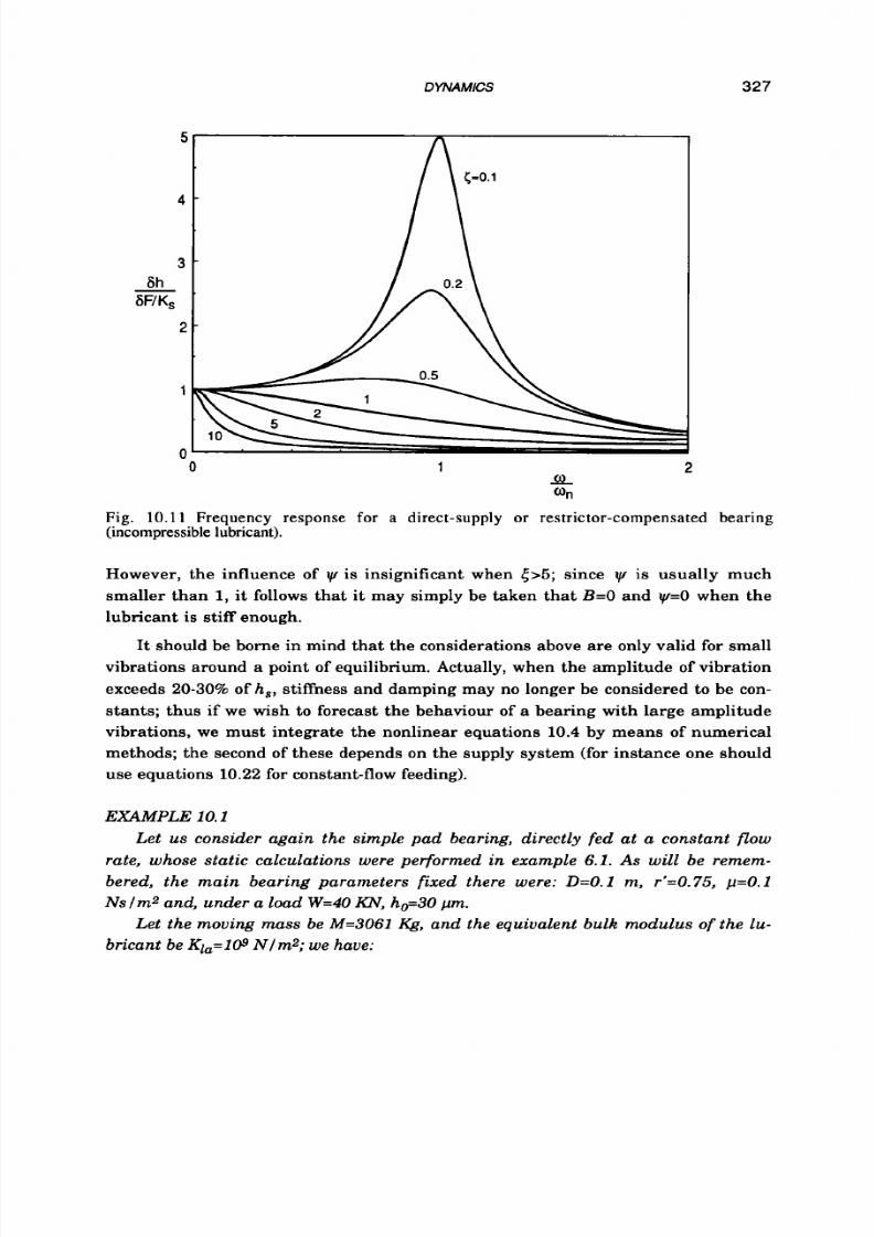
8/9/2019 Hydrostatic Lubrication 1992
http://slidepdf.com/reader/full/hydrostatic-lubrication-1992 344/558
DYNAMICS 327
0
1 2
L L
a n
Fig.
10.11
Frequency response
for
a direct-supply or restrictor-compensated bearing
(incompressible lubricant).
However, the influence of w is insignificant when
5>5;
since
w
is usually much
smaller than
1,
it follows that it may simply be taken that
B=O
and
w=O
when the
lubricant is
stiff
enough.
It should be borne in mind tha t the considerations above are only valid for small
vibrations around a point of equilibrium. Actually, when the amplitude of vibration
exceeds 20-30%of h,, stiffness and damping may no longer be considered to be con-
stants; thus if we wish to forecast the behaviour of a bearing with large amplitude
vibrations, we must integrate the nonlinear equations
10.4
by means of numerical
methods; the second of these depends on the supply system (for instance one should
use equations 10.22 for constant-flow feeding).
EXAMPLE 10.1
Let
us
consder again the simple pad bearing, directly fed at a constant flow
rate, whose static calculations were performed i n exam ple 6.1. As will be remem-
bered, the main bearing parameters fixed there were: D=O.l m,
r’=O.75,
p=O.1
Ns
1
m2 and, u nder a load
W=40
N , ho=30 pm.
Let th e moving
mass
be M=3061
Kg,
nd the equivalent bulk modulus of the
lu-
bricant be Kla=109N lm 2; we have:
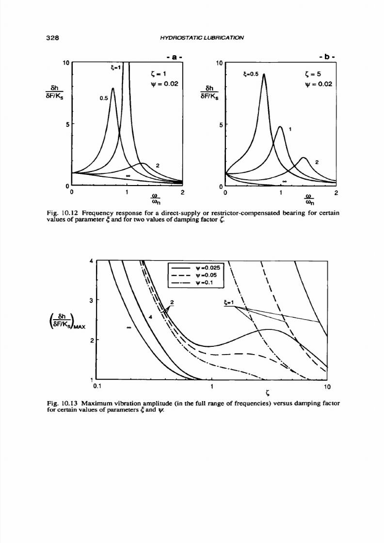
8/9/2019 Hydrostatic Lubrication 1992
http://slidepdf.com/reader/full/hydrostatic-lubrication-1992 345/558
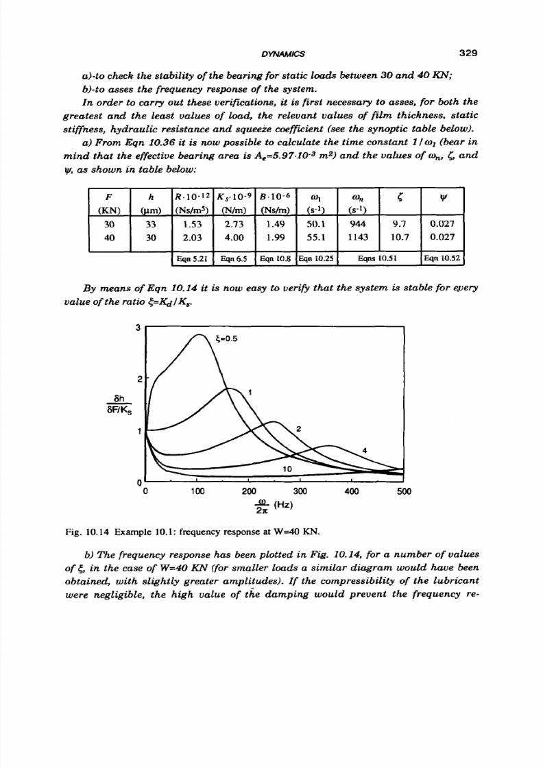
8/9/2019 Hydrostatic Lubrication 1992
http://slidepdf.com/reader/full/hydrostatic-lubrication-1992 346/558
DYNAMICS
F h R . I O - ~ Z ,.10-9
. I O - ~ w1
w,
(KN)
urn) (Ns/rn5)
(N/m)
(Ns/m) (s-1)
( s l )
30
33
1.53
2.73 1.49
50.1
944
40 30 2.03 4.00 1.99
55.1 1143
329
c
w
9.7 0.027
10.7 0.027
ah to check the stability of the bearing for static loads between 30 and 40m;
b)-to asses the frequency response o f the system.
In order to carry out these verifications, it
is
first necessary to asses, for both th e
greatest and the least values of load, the relevant values of fi l m thickness, static
stiffness, hydraulic resistance and squeeze coeffEient (see the synoptic table below).
a) From Eqn 10.36 it
is
now possible to calculate the t im e constant
1
ol (bear in
min d tha t the effective bearing area isA,=5.97.103ma) and the values of %,
&
and
as
shown
in table below:
Eqn 5.21 Eqn
6.5
Eqn 10.8
Eqn 10.25
Eqns
10.51
Eqn 10.52
By means of Eqn 10.14 it
is
now easy to verify tha t the system
is
stable fo r every
value
of
the ratio &IQ I Kw
3
2
6h
6WKS
-
1
0
1
0 100
200
300
400 500
Fig. 10.14 Example 10.1:requency response
at
W& KN.
b)
Th e frequency response has been plotted i n Fig. 10.14, or a number of values
o f
(,
i n th e case of
W=40
N
(for smaller
loads
a similar diagram would have been
obtained, with slightly greater amplitudes). If the compressibility of the lubricant
were negligible, the high value
of
the damping would prevent the frequency re-

8/9/2019 Hydrostatic Lubrication 1992
http://slidepdf.com/reader/full/hydrostatic-lubrication-1992 347/558
330 HYDROSTATIC LUBRICATION
F
(KN)
20
35
sponse from the presence of peaks, which, on the contrary, may be notable for val-
ues of 5 lower than 1. This means that supply pump should be very close to the bear-
ing. For instance, in order to have <>1, lubricant stiffness Kd should be greater than
4.109 Nl m : it follows from Eqn 10.19 that the volume of lubricant in the recess and
supply pipes should be smaller than 8.9.10-6 m3.
It is easy to see that, in order to increase
<,
one could try to increase slightly the
fi lm thickness or the effective area of the bearing. In the first case greater flow rate
and pumping power would be required, while stiffness and damping factor would
turn out to be lowered. In the latter case, on the contrary, a great increase in lubri-
cant stif fness (namely, parameter
5
proves to be proportional to the fourth power of
D )
would match a consistent reduction in flow rate, supply pressure and total power
(because turning speed is
low); damping factor, too, would be greater.
P h prlps d Ks.10-9
<
w,,
C
Y
(Ns/m*) urn) (N/m)
@-I)
0.015 40
0.437 1.78
0.845 3.87 650
0.196 0.003
0.015 24.8
0.765
4.25 0.995
3.29
705 0.315 0.007
EXAMPLE 10.2
The pad bearing already considered in Example 6.4 bears a load W0=20
K N ,
with
a clearance ho=40 pm, when fed at
a
constant pressure ps=4 MPa through a com-
pensating restrictor, with a pressure ratio p=0.437. Under a load W ~ = 3 5N , clear-
ance is reduced to 24.8 ,um and pressure ratio rises up to 0.765.
Assuming that moving mass is M=2000h that the equivalent bulk modulus of
lubricant is Kla=500 MNI m2 and that the lubricant volume comprised between the
restrictor and the pad clearances
is
V=20.10-6m4
we
have to check for stability and
to assess the frequency response
o f
the system.
From Example 6.4 we get: D=0.16 m2, r'=O.625, a'=0.067, A,=O.0114 m2,
R*=0.0154. Hydraulic resistance R may
be
calculated from Eqn 5.68, squeeze coeffi-
cient
B
from Eqn 10.12, parameter
w*
rom Eqn 10.9 (or
from
Fig. 10.4.b), static stiff-
ness
K,
from Eqn 10.30, while lubricant stiffness Kd is given by Eqn 10.19, in which
the contribution o f the compliance of supply pipe may be disregarded. The main
dynamic parameters can now be evaluated, as shown in table below.
Eqn 10.29 Eqn 10.30 Eqn 10.54 Eqns 10.51 Eqn 10.52
Stability is clearly out of question,
since
5>1; the linearized frequency response
has been plotted for both the greatest and the least loads in Fig. 10.15. Comparing
this diagram with the frequency response in the case of incompressible lubricant
(Fig. 10.11) it should be evident that compressibility produces a noticeable decrease

8/9/2019 Hydrostatic Lubrication 1992
http://slidepdf.com/reader/full/hydrostatic-lubrication-1992 348/558
DYNAMICS
4
331
Fig. 10.15
Example
10.2:
frequency response.
in damping, that
is
the amplitude
of
oscillation in the neighborough
of
resonance is
greater. In order to reduce the peaks of vibration one should increase 5 and, above
all,
c.
This may be obtained reviewing the design and using,
if
possible,
a
slightly
larger pad.
10.6 OPPOSED-PAD BEARINGS
Opposed-pad thrust bearings (Fig. 7.1)may be regarded as a set of two single-
effect pad bearings. For the sake of convenience, the position of the moving member
which divides the axial playg into two equal parts may be taken as reference;
hence,
hlo=h20=ho=g12.or
the two pads, we have (see Eqns 7.4):
hl
-ho
& 1 = h = &
,
0
(10.62)
If each pad is supplied independently (e.g. by two pumps or through two restric-
tors), the relevant block diagram can be obtained by summing the effects of both
components (Fig. 10.16).The equation of motion may be obtained from the balance of
forces acting on the moving member:
By linearizing, Laplace-transforming and bearing in mind t ha t (as follows from
previous sections):

8/9/2019 Hydrostatic Lubrication 1992
http://slidepdf.com/reader/full/hydrostatic-lubrication-1992 349/558
332
HYDROSTATIC LUBRlCA
TION
Fig. 10.16 Block diagram for opposed-padbearings.
equation 10.63 becomes:
M
ho S ~ S E
(B1, +
B a )ho
s
BE+
(Ae, &I +Ae2 &2)
S E =
6F
(10.64)
(10.65)
Squeeze coefficients
B1,
and
Bas
can be calculated from the results in section 10.4,
while blocks jLP have been the matter of section 10.5.
In what follows, symmetrical bearings alone (i.e.
Ael=Aez=Ae
and
R ~ ( E ) = R ~ ( - E ) )
will be studied in a greater detail.
For
such bearings the block scheme in
Fig.
10.16
may be substituted by the one in Rg. 10.17; the latter is valid even when the two re-
cesses are not supplied by independent devices (e.g. when a flow divider
is
used),
after the relevant expression for
&
has been found. In the case of symmetrical bear-
ings, Eqn 10.65 may be rewritten as:
M
ho
s2&+ B,
ho
s
& + A e
jLP
8 ~ =
F
(10.66)
Fig. 10.17 Block diagram for symmetrical opposed-padbearings.

8/9/2019 Hydrostatic Lubrication 1992
http://slidepdf.com/reader/full/hydrostatic-lubrication-1992 350/558
DYNAMICS
333
10
B
5 -
0
and, thus, the relevant transfer function is formally identical to Eqn 10.7.Block
&
is
clearly the sum of AP1 and APz. The squeeze coefficient may be calculated from the
following equation:
-
1
where Bo has the same value as each pad (for example, for circular bearings, see
Fig. 10.41,while B' is given (for pads having uniform film thickness) by
A plot of B' is also given in Fig.
10.18.
(10.68)
10.6.1 Direct supply (constant f low)
flow Q / 2 , we have:
When each recess is supplied independently by a pump delivering a constant
(10.69)
S
1+ (1 &)-
5P2
Koho 1
w1
(1-EY 2
42'
-= -
E
2Ae
-
+ 1 s
where:
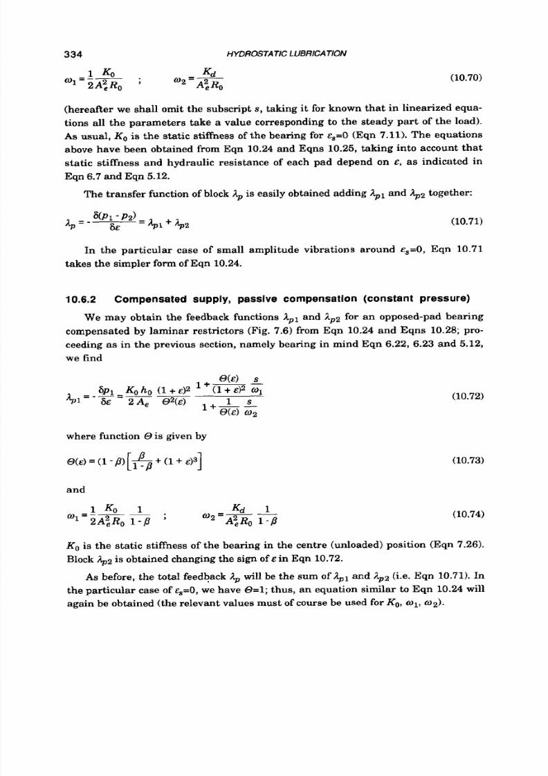
8/9/2019 Hydrostatic Lubrication 1992
http://slidepdf.com/reader/full/hydrostatic-lubrication-1992 351/558
334
HYDROSTATIC LUBRICATION
(10.70)
(hereafter we shall omit the subscript s, taking i t for known that in linearized equa-
tions all the parameters take a value corresponding to the steady part of the load).
A s usual, KO s the static stiffness of the bearing for E,=O (Eqn
7.11).
The equations
above have been obtained from Eqn
10.24
and Eqns
10.25,
taking into account tha t
static stiffness and hydraulic resistance of each pad depend on
E ,
as indicated in
Eqn
6.7 and
Eqn
5.12.
The transfer function of block
&
is easily obtained adding &1 and h2ogether:
(10.71)
In the particular case of small amplitude vibrations around cS=O, Eqn
10.71
takes the simpler form of Eqn
10.24.
10.6.2
Compensated supply, passive compensation (constant pressure)
We may obtain the feedback functions ;Ipl and Ap2 for an opposed-pad bearing
compensated by laminar restrictors (Fig.
7.6)
from Eqn
10.24
and Eqns
10.28;
pro-
ceeding
as
in the previous section, namely bearing in mind Eqn
6.22, 6.23
and
5.12,
we find
(10.72)
where function
0
s given by
=
(1
-P)
A
(1
+
(10.73)
and
(10.74)
KO s the static stiffness of the bearing in the centre (unloaded) position (Eqn
7.26).
Block
4 2
s obtained changing the sign of
E
in Eqn
10.72.
As
before, the
total
feedback
,$
will be the sum of
jZpl
and ;Lpa
(i.e.
Eqn
10.71).
In
the particular case of
eS=O,
we have
0=1;
thus, an equation similar
to
Eqn
10.24
will
again be obtained (the relevant values must of course be used for KO, 1 ,2 ) .
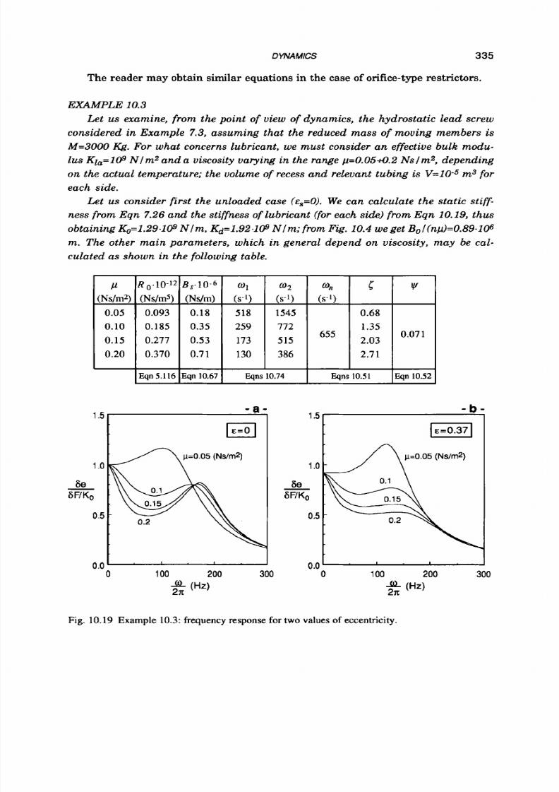
8/9/2019 Hydrostatic Lubrication 1992
http://slidepdf.com/reader/full/hydrostatic-lubrication-1992 352/558
DYNAMlcS
335
P,.10-'2
(NsIm5)
0.093
0.185
0.277
0.370
Eqn 5.116
The reader may obtain similar equations in the
case
of orifice-type restrictors.
B,-10-6
o1 w2 on 5 w
(Ns/m)
(s-1) (s-1) (s-1)
0.18 518 1545 0.68
0.35 259 772 1.35
0.53
173 515
655
2.03
0.71 130 386 2.7 1
0.07 1
Eqn
10.67
Eqns
10.74
Eqns 10.51
Eqn
10.52
E W P L E 10.3
Let us examine, from the point
of
view
o f
dynamics, the hydrostatic lead screw
considered
in
Example 7.3, assuming that the reduced mass
of
moving members is
M=3000I@. For what concerns lubricant, we must consider an effective bulk modu-
lus Kla=109N lm z an da viscosity varying in the range p=0.05+0.2 Nslm2, depending
on the actual temperature; the volume of recess and relevant tubing is V=10-5
m3
for
each side.
Let us consider first the unloaded case
(E~=O).
We can calculate the static s ti ff -
ness from Eqn 7.26 and the stiffness of lubricant (for each side) from Eqn 10.19, thus
obtaining K0=1.29.1# N lm , Kd=1.92.1@ Nlm; rom Fig. 10.4 weget Bol(np)=0.89.106
m. The other
main
parameters, which in general depend on viscosity, may be cal-
culated as shown in the following table.
- b -
1 . 5 1
1
o
0.5
0.0
I 1 I
0 100 200
300
Fig. 10.19 Example 10.3: frequency response for two values
of
eccentricity.
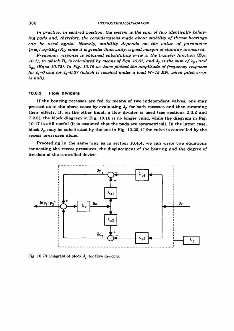
8/9/2019 Hydrostatic Lubrication 1992
http://slidepdf.com/reader/full/hydrostatic-lubrication-1992 353/558
336
HYDROSTATIC L UBRlCATiON
I n practice,
in
centred position, the system
is
the s um of two identically behav-
ing pad s and , therefore, the considerations m ade about stability o f thru st bearings
can be used again. Name ly, s tabi l i ty depends on the value of param eter
t=%/
l=2KdlK&
ince it
is
greater tha n unity, a good margin o f stability is ensured.
Frequency response is obtained substituting s=iw in the tra nsfer funct ion (Eqn
10.71,
n
which B, s calculated by means o f Eq n 10.67, nd ;\p
is
t he sum o f ;\pl and
App2 (Eqns 10.72). I n Fig. 10.19 we have plotted the amplitude of frequency response
for
E,=O and for
~,=0.37
which is reached under a load W=l5 P& when pitc h error
is null).
10.6.3 Flow
dividers
If the bearing recesses are fed by means of two independent valves, one may
proceed
as
in the above cases by evaluating Ap for both recesses and then summing
their effects. If, on the other hand, a flow divider is used (see sections 2.3.2 and
7.2.51, the block diagram in Fig. 10.16 is no longer valid, while the diagram in Fig.
10.17
s still useful (it
is
assumed that the pads are symmetrical). In the latter case,
block may be substituted by the one in Fig. 10.20, if the valve
is
controlled by the
recess pressures alone.
Proceeding in the same way
as
in section
10.4.4,
we can write two equations
connecting the recess pressures, the displacement of the bearing and the degree of
freedom of the controlled device:
I
I
I
I
I
I
I
I
I
I
I
I
I
: t i €
I
I
I
I
I
I
I
I
I
I
I
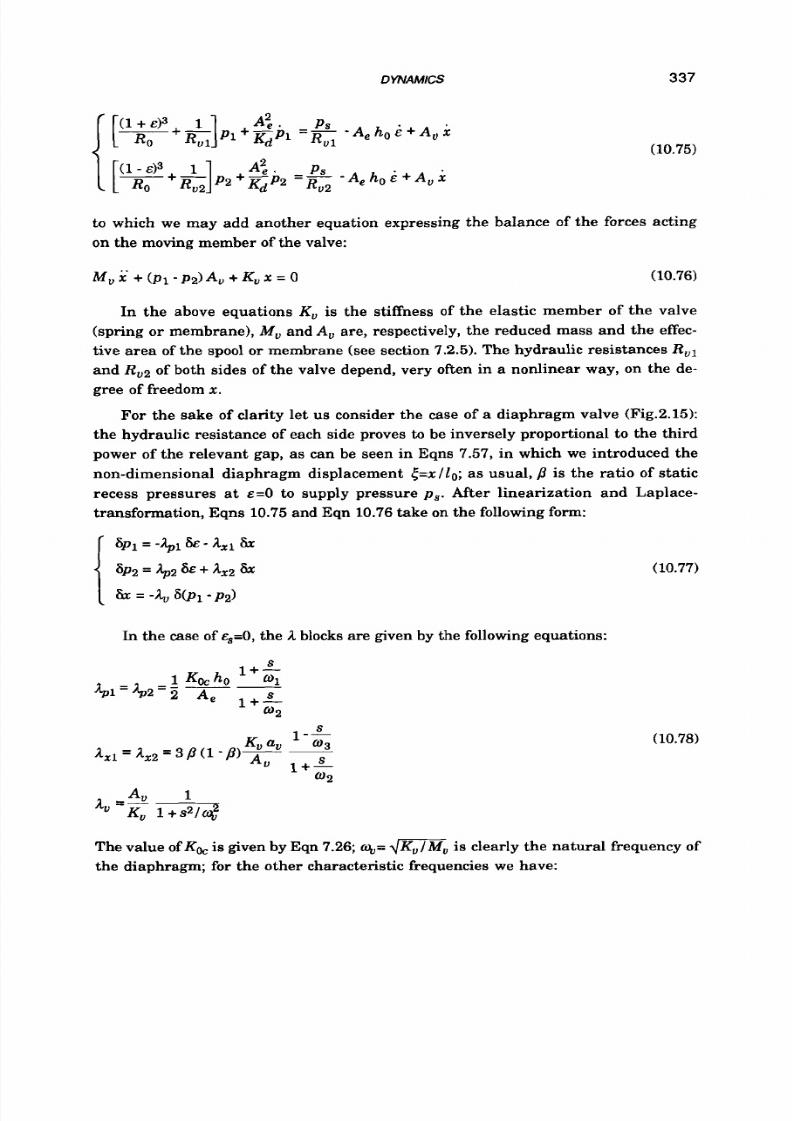
8/9/2019 Hydrostatic Lubrication 1992
http://slidepdf.com/reader/full/hydrostatic-lubrication-1992 354/558
DYNAMICS
337
(10.75)
to which we may add another equation expressing the balance of the forces acting
on the moving member of the valve:
In the above equations
K ,
is the stiffness of the elastic member of the valve
(spring
o r
membrane),
M ,
and
A ,
are, respectively, the reduced mass and the effec-
tive area of the spool
o r
membrane (see section 7.2.5). The hydraulic resistances R,1
and R v 2 of both sides of the valve depend, very often in a nonlinear way, on the de-
gree of freedom
x .
For the sake of clarity let us consider the case of
a
diaphragm valve (Fig.2.15):
the hydraulic resistance of each side proves to be inversely proportional to the third
power of the relevant gap, as can be seen in Eqns
7.57,
n which we introduced the
non-dimensional diaphragm displacement <=x / l o ;as usual, p is the ratio of static
recess pressures at
E=O
to supply pressure
p s .
After linearization and Laplace-
transformation, Eqns
10.75
and Eqn
10.76
take on the following form:
In
the case of
~~'0,
he A blocks are given by the following equations:
(10.77)
S
1 -
"3
1+-
"2
S
(10.78)
The value of KW is given by Eqn
7.26;q,=
w u s clearly the natural frequency of
the diaphragm; for the other characteristic frequencies we have:
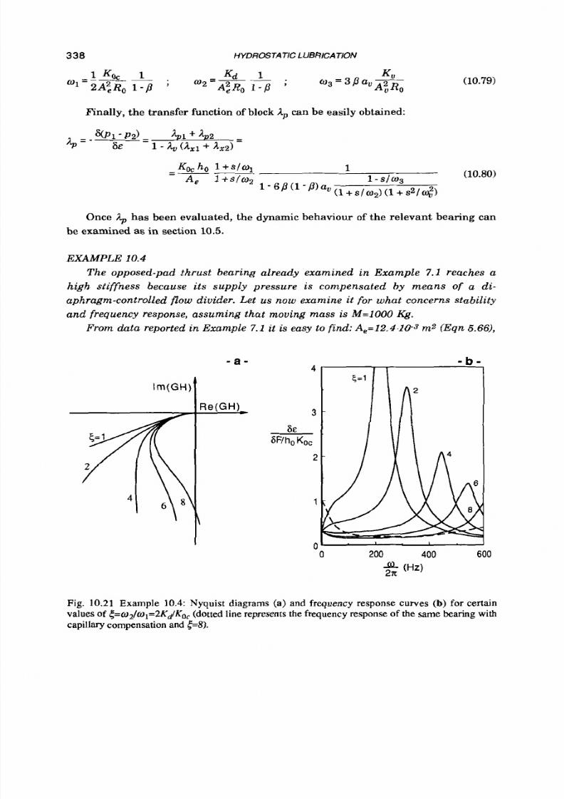
8/9/2019 Hydrostatic Lubrication 1992
http://slidepdf.com/reader/full/hydrostatic-lubrication-1992 355/558
338 HYDROSTATIC LUBRICATION
(10.79)
Finally, the transfer function of block
,Ip
can be easily obtained:
Once & has been evaluated, the dynamic behaviour of the relevant bearing can
be examined as in section 10.5.
EXAMPLE 10.4
T h e opposed-pad thrust bearing already examined in Example
7 . 1
reaches a
hig h s t i f fness because i t s supply pressure i s compensated
by
m e a n s o f a d i -
aphragm-controlled
flow
divider. Let
us
now examine
it
for wh at concerns stability
and frequency response, assuming that moving mass is
M=lOOO @.
From data reported in Example
7 .1
it is easy to find:
A,=12.4.10-3 m2
( E q n
5.66),
- a -
R e ( G H )
\
- b -
0 '
I
0
200 400 600
$$ ( H a
Fig.
10.21
Example
10.4:
Nyquist diagrams (a) and frequency response curves (b) for certain
values of
{=w2/w,=2Kd/KOc
dotted line represents the frequency response o f the sam e
bearing
with
capillary compensation and <=S).
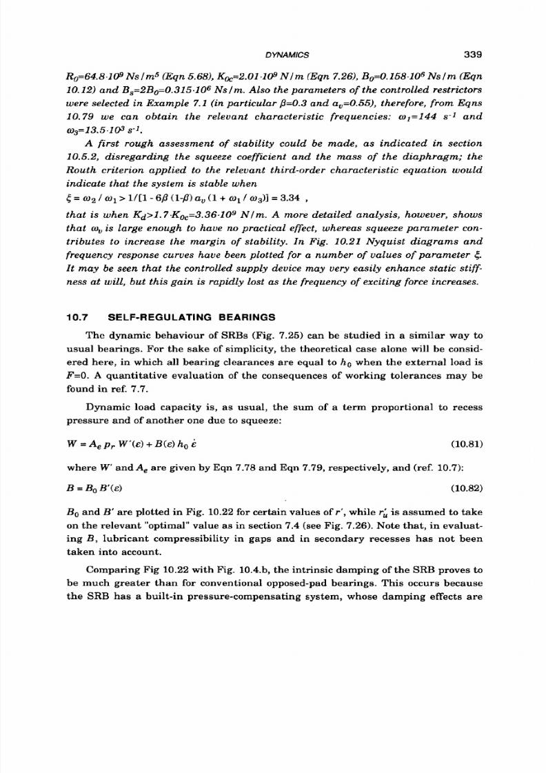
8/9/2019 Hydrostatic Lubrication 1992
http://slidepdf.com/reader/full/hydrostatic-lubrication-1992 356/558
DYNAMICS 339
Ro=64.8.109Ns lm5 (Eqn5.68), Kk=2.01.109 N l m (Eqn 7.26),B0=0.158.106Ns lm (Eqn
10.12) and B,=2Bo=0.315.106 Nslm. Also the parameters of the controlled restrictors
were selected in Example 7.1 (in particular 8=0.3 and a,=0.55), therefore, from Eqns
10.79
we can obtain the relevant characteristic frequencies:
W1=144
s-1
and
A first rough assessment of stability could be made, as indicated in section
10.5.2, disregarding the squeeze coefficient and the mass o f the diaphragm; the
Routh criterion applied to the relevant third-order characteristic equation would
indicate that the system is stable when
5 = w 2
/
o1
1/[1- @ 1-P)a,
(1 + w 1 / 03 1
3.34 ,
that is when Kd>l.7~Koc=3.36~109lm . A more detailed analysis, however, shows
that
w,
is large enough to have no practical effect, whereas squeeze parameter con-
tributes to increase the margin of stability. In Fig. 10.21 Nyquist diagrams and
frequency response curves have been plotted
for
a number of values
of
parameter 4.
It may be seen that the controlled supply device may very easily enhance static stiff-
ness at will, but this gain is rapidly lost as the frequency of exciting force increases.
03=13.5.1@s'.
10.7 SELF-REGULATING BEARINGS
The dynamic behaviour of SRBs (Fig. 7.25) can be studied in a similar way to
usual bearings.
For
the sake
of
simplicity, the theoretical case alone will be consid-
ered here, in which all bearing clearances are equal to ho when the external load is
F=O.
A
quantitative evaluation of the consequences of working tolerances may be
found in ref. 7.7.
Dynamic load capacity is, as usual, the sum of
a
term proportional to recess
pressure and of another one due to squeeze:
W = A ,p,. W ' ( E ) B(E)o
&
(10.81)
where
W
and A, are given by Eqn 7.78 and Eqn 7.79, respectively, and (ref. 10.7):
B =
Bo
B'(E)
(10.82)
Bo and B' are plotted in Fig. 10.22 for certain values of r', while
rh
is assumed to take
on the relevant "optimal" value as in section 7.4 (see Fig. 7.26). Note that , in evaluat-
ing
B,
lubricant compressibility in gaps and in secondary recesses has not been
taken into account.
Comparing Fig 10.22 with Fig.
10.4.b,
the intrinsic damping of the SRB proves
t o
be much greater than for conventional opposed-pad bearings. This occurs because
the SRB has a built-in pressure-compensating system, whose damping effects are
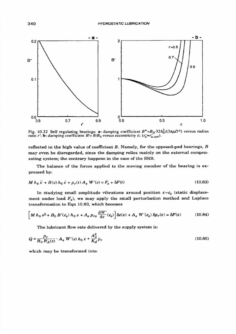
8/9/2019 Hydrostatic Lubrication 1992
http://slidepdf.com/reader/full/hydrostatic-lubrication-1992 357/558
340
HYDROSTATIC LUBRICATION
- b -
B*
0
2
B
1
.
0.5
0.7
0.9
I
I"
0.5
1 o
E
Fig. 10.22 Self regulating bearings: a- damping coefficient
B*=B0.32h30/(3x/d)4)
versus radius
ratio
r ' ; b-
damping coefficient B'=
BIB,
versus eccentricity
E ; ( r i=r i , op t ) .
reflected in the high value of coefficientB. Namely, for the opposed-pad bearings, B
may even be disregarded, since the damping relies mainly on the external compen-
sating system; the contrary happens in the case of the SRB.
The balance of the forces applied
to
the moving member
of
the bearing is ex-
pressed by:
In studying small amplitude vibrations around position E = E ~ (static displace-
ment under load
Fs),
e may apply the small perturbation method and Laplace
transformation to
Eqn 10.83,
which becomes
The lubricant flow rate delivered by the supply system is:
(10.85)
which may be transformed into:

8/9/2019 Hydrostatic Lubrication 1992
http://slidepdf.com/reader/full/hydrostatic-lubrication-1992 358/558
D WA
MlCS 341
(10.86)
(Equations
for
Ro
nd
R i
are given in section
7.4).
10.7.1
Constant f low feeding
The behaviour of the system is represented by Eqn
10.83
and Eqn
10.85
in which
Q is
assumed to be a constant. In the case of small amplitude vibrations, Eqn
10.84
and Eqn
10.86
may be used instead, and SQ=O. Equation
10.86
leads to:
where
Kd
e O
" 2 = = ;
KO
1 = - 2 '
3A,Ro '
(10.87)
(10.88)
KO
s
the bearing stiffness in the unloaded configuration (Eqn
7.92),
Kd is the
stiff-
ness of lubricant contained in the central recess and in the relevant supply pipes
(Eqn
10.19);
coefficients G1 nd
G2
are non-dimensional functions of the displace-
ment, given in Fig. 10.23. It should be noted that if the static part
of
the load is null,
;lp
also vanishes.
The transfer function
of
the whole system is (from Eqn 10.84):
where
(10.89)
K
is given by Eqn
7.93
(and Fig.
7.27),
coefficients
G2
and G3 re plotted in Fig.
10.23
as functions of the static displacement. It is easy to see that, for static loads
(s=O),
Eqn 7.91 is again obtained.

8/9/2019 Hydrostatic Lubrication 1992
http://slidepdf.com/reader/full/hydrostatic-lubrication-1992 359/558
342
100
Gl
10
1
0.'
HYDROSTATIC LUBRICATION
- a -
0
o
0.5 1
o
E
- b -
11
G2
G3
O
0.1
0.5
1
o
E
Fig. 10.23 Self-regulating bearings: coefficients G , , G 2and G 3 versus eccentricity.
When the sta tic load is null, we get G3=0 nd
K'=l;
hence, the bearing behaves
like a second order system with undamped natural frequency 0 ~ 1 2 ~nd a damping
factor
c.
In general cases, it will be a three-pole system.
For
what concerns stability, it is easy to see that no problem generally exists,
even when { = w , / q is small, since the damping properties of the system rely mostly
on the bearing itself (namely on coefficient B ) rather than on the supply system.
10.7.2 Constant pressure feeding
When the SRB is directly fed by a hydraulic network at constant pressure p s , we
shall obviously have
p r = p s
and
6 p r = 0 .
Hence, the behaviour of the system is de-
scribed by Eqn
10.83
or, in the case of the linearized model, by Eqn
10.84
which may
be written as follows:
(10.91)
where KO s the static stiffness in the centre position (Eqn 7.97) and K is given by
Eqn
7.98.
Note that, under the simplifying assumptions we have made, lubricant
compressibility has no influence on the dynamic behaviour of the bearing, which is
reduced to a second order system.

8/9/2019 Hydrostatic Lubrication 1992
http://slidepdf.com/reader/full/hydrostatic-lubrication-1992 360/558
DMvAMlCS 343
When the
SRB
is fed through a laminar-flow restrictor
R,
(see section 7.4.21, the
variation in flow rate due to a change in recess pressure is
which can be substituted in Eqn 10.86 t o obtain the feedback function
Ap=6p,./8&.
Then, the transfer function may be obtained from Eqn 10.84. In this case, too, we get
a second-order system when the static part of the load is null.
10.8
MULTIPAD
BEARING SYSTEMS
This section deals with the hydrostatic bearing systems consisting of a certain
number of independent pads, which are able to sustain loads in multiple directions.
The multipad journal bearing in Fig. 1.12.a and the hydrostatic slideway in Fig.
1.16 are examples of such systems. In the first example the bearing is able to SUS-
tain loads along any radial direction; hence, its displacement may be described by a
set of two coordinates. In the second case, the 12 hydrostatic pads take the loads in
every direction, except along the x: axis: five coordinates (and five equations) will
therefore be required to describe the static and dynamic behaviour of the carriage.
In every case the system may be studied along the following lines:
i) first, we must fix a suitable set of n generalized (Lagrangian) coordinates,
able
to
describe any displacement of the system: obviously,
n
is the number of
degrees of freedom constrained by the bearing system;
ii) we must obtain an equation for each pad, giving
its
dynamic load capacity
Wj as
a
function of the parameters which characterize the supply system, of
the generalized coordinates and of their time-derivatives;
iii) we must write down a set of n independent differential equations, express-
ing the balance of the external forces, of the inertia forces and of the load
capacities (D'Alembert
o r
Lagrange equations). In general,
a
complicated
set of nonlinear equations will be obtained, requiring numerical simulation
to trace the system response to large-amplitude loads. In most case, how-
ever, it will be enough to linearize these equations and to examine them to
judge the stability of the system and
t o
obtain its response t o dynamic loads.
A number of other considerations must be borne in mind in certain cases. For
instance, when the tangential speed is high and the thickness of the film of lubri-
cant
is
not uniform,
as
happens in journal bearings, the forces due to the hydrody-
namic effect should be taken into account.
8/9/2019 Hydrostatic Lubrication 1992
http://slidepdf.com/reader/full/hydrostatic-lubrication-1992 361/558
344 H YDRCSTATIC LUBRICATION
10.8.1
Hydrostatic slideways
Let us now see, with the aid of a practical example, how the dynamic study of a
system of pads may be stated. The simple carriage sketched in Fig. 7.29 is supported
by four hydrostatic plane pads. In any given steady configuration, the mean film
thickness of the j-th pad
is hjo
and
e&-hjo)/hj0
is the relative variation of the gap.
Each pad exerts on the carriage a force
Wj,
that may be written in the following
form:
W j
=
Aj pj
-
BjC&j)hjo
Ej
Cj= 1 ...m )
(10.92)
The effective area
Aj
may be considered to be a constant; actually certain displace-
ments of the carriage may make the bearing surfaces out of parallel, and conse-
quently may affect the coeficient
Aj:
however, such changes are generally negligi-
ble. The squeeze coefficient
Bj
is greatly affected by the actual value of the film
thickness; on the other hand, as already noted in section 10.5, initially
it
can be to-
tally disregarded; alternatively, it may be substituted by
its
reference value
Bjo=Bj(0),
hen small displacements from the steady configuration are considered.
The equations of motion of such systems can be obtained equating the external
forces to the inertia forces; their general form is, therefore:
(z = 1
..
n)
where m is the number of pads, n the number of generalized coordinates
(10.93)
x i
6.e. the
degrees of freedom constrained by the pads); the terms auWj are the generalized
components of the pad forces, i.e. aii=hjo.(dej/dxi),nd
Fi
are the generalized com-
ponents of the external forces. In the case of the system in Fig. 7.29, it is clearly
m=4, n=3; the xi are the axis z and the tilt angles 8, and 8,; therefore Eqns 10.93
become:
-M +
C,Wj)
+
Fz
= 0
-J, 8, + b ( W , +Wz -W3 -W4)+M, = 0
J
I-J,
8
-
a (w,
w,
-w3 w 4 )+ M,
= o
(it is assumed that x , y and z are principal axes). The Ji are the inert ia moments,
the Fi and Mi are the components of the resultant and of the resultant moment of
the external forces. The forces
Wj
are given by Eqns 10.92, in which the recess pres-
sures
p j
are still unknown. If each pad is fed by a n independent supply device, each
pressure
p , is
related
to
the relevant displacement 5 by an equation

8/9/2019 Hydrostatic Lubrication 1992
http://slidepdf.com/reader/full/hydrostatic-lubrication-1992 362/558
DYNAMICS 345
like the ones already examined in section
10.4.
Of course, if the supply devices are
not independent (for instance when flow dividers are employed), more complicated
relations are needed, the general form being:
(10.95)
The pad displacements ~j may be written as functions of the Lagrangian coordi-
nates:
For
instance, for the system in Fig.
7.29,
we have:
1
E~ = (Z
+ b
0, - a eY)
Q
=g
(z
+ 6 0,
+
a OY)
1
and so on.
If we introduce Eqns
10.92
and Eqns
10.96
into Eqns
10.93,
hese last , together
with Eqns
10.94 (or,
more generally, Eqns
10.95))
onstitute a set of non-linear dif-
ferential equations that are clearly difficult to handle. As usual, a very great simpli-
fication is obtained by limiting ourselves to studying the system for the case of small
vibrations. It is possible, therefore, to linearize and Laplace-transform the foregoing
equations. ARer the transformation, Eqns
10.94
may be written in the form:
spj =
-&jW
6Ej
(10.97)
Functions Apj of the complex variable s may be written as in section
10.4,
de-
pending on the type of supply device. Typically, each
&j
can be written in the form of
Eqn
10.24,
n which
w 1
and w 2 are given by Eqns
10.25
when multiple pumps are
used, or by Eqns
10.28
or restrictor compensation. A couple of opposite pads may be
treated also as a single opposed-pad bearing, especially when compensated by
means
of
a controlled restrictor: in this case, h j will be obtained as indicated in sec-
tion
10.6.
Equations
10.92
now become
SWj = - [Aj APj(s)
+
Bj hjo
S]
&j
(10.98)
and, thanks to Eqns
10.96,
may further be written in terms of the coordinates
x i ,
instead of the
~ j .

8/9/2019 Hydrostatic Lubrication 1992
http://slidepdf.com/reader/full/hydrostatic-lubrication-1992 363/558
346 HYDROSTATIC LUBRICATION
Finally, by linearizing Eqns 10.93, a set of n linear equations
is
obtained which
constitutes a model of the dynamic behaviour of the carriage. For instance let us
consider again the system in Fig. 7.29, with some further simplifications: all the
pads a re equal ( the same values for the effective area
A,,,
and the same clearance
ho
in the steady configuration) and are fed through capillary restrictors with the same
pressure ratio 8 . Equations 10.98 now give (see section 10.4.2):
Bo
1+s/w1
KO
here
A = - s + l + s / o z
and
w1
and
0 2
are given by Eqns 10.28. Proceeding as outlined above, the following
set of equations is obtained:
M s ~ &
4
KO
A & =
SF,
J , ~ 2 6 0 ~4 b2Ko
A
60,
=
W x
J Y s 2
66, +
4a2 KO 6ey
= SM,
These equations are completely uncoupled: obviously this is only a consequence
of the simplicity of the system we have considered and will not be generally ob-
tained. If the lubricant is sufficiently stiff (w2>>w1), the operator A
becomes
A=1+ (l/q+Bo/&)s. No stability problem should hence exists: indeed, this kind of
systems often feature a great damping.
10.8.2 Mult ipad journal bearings
Let us now consider a journal bearing made up of
n
cylindrical pads (Fig.10.24),
Fig.
10.24 Multipadjournal bearing.
8/9/2019 Hydrostatic Lubrication 1992
http://slidepdf.com/reader/full/hydrostatic-lubrication-1992 364/558
DYNAMICS 347
that may completely surround the shaft. The actual position of the shaft axis, with
reference to the centred configuration, may be defined by two non-dimensional
coordinates: < = x / C and q = y / C . The general problem is quite difficult: the hydraulic
resistance
Ri
and the load capacity
Wi
of each pad show a nonlinear dependence on
the shaft displacement and on its velocity; Wi
is
not always directed toward the cen-
tre of the bearing, but a tangential component may exist; furthermore, the Reynolds
equation may not be directly solved, and hence numerical computing should be used
to obtain load and flow rate.
However, if the displacement is not
too
great
( E c O . ~ ) ,
if the arc taken by each pad
is smaller than
90°
and the turning speed of the journal is not so high as to give
appreciable hydrodynamic effects, great simplifications can be introduced.
First
the
tangential component of the load capacity may be disregarded:
Wi
is directed as
~ i .
Then it may be assumed that the load capacity and hydraulic resistance of the i-th
pad depends only on the relevant components
of
the shaft displacement and velocity,
namely on
~i
and
E i .
The load capacity of each pad may be written in the usual form
The effective area A, may be considered a constant (see section
5.8).
The coefficient
Bi
depends mainly on the clearance:
a
rough evaluation
is
often enough; it may
even be totally disregarded.
The relevant perturbation is, therefore,
SWi
=A,
Spi -
Bi,
C
s
6 ~ i
(10.100)
The perturbation of each recess pressure may be written in the usual form (Eqn
10.97) and each operator
$(s)
obtained as shown in the preceding sections. For
instance, in the classical case of capillary compensation (see also section
10.6.2)
we
obtain:
where KO (reference stiffness of each pad) is given
by
Eqn 6.22,
w 1
and
o2
re given
by Eqn 10.28 and O(E) y Eqn
10.73
(hereafter we shall omit the subscript "s",by
which we mean that all the parameters are calculated in the point of sta tic equilib-
rium). If
n
is an even number,
it
may be preferable to consider the multipad bearing
as a set of
n/2
opposed-pad bearings, obtaining the operators as in section
10.6.
In
any case, Eqn
10.100
becomes
8/9/2019 Hydrostatic Lubrication 1992
http://slidepdf.com/reader/full/hydrostatic-lubrication-1992 365/558
348
HYDROSTATIC LUBRICATION
(10.101)
The equations of motion for the journal may now be easily written:
(10.102)
where
W t
and 6Fq are the components of the external perturbation.
A t this point the problem is completely defined, for we have a set of differential
equations connecting the displacement of the journal to the external excitation. In
facts, it is easy to see that the pad displacements S E ~ epend on the journal dis-
placement:
(10.103)
Introducing Eqns 10.101 and Eqn 10.103 into Eqn 10.102, the equations of motion
become:
(10.104)
Apparently, this is a complicated set of equations; in particular cases, however con-
siderable simplifications can be introduced: for instance, if we assume that n=4,
&=O, and that
5
is directed toward the centre of a pad, i t is very easy to see that the
above set splits into two independent equations:
Very simple equations are obtained in the case of small vibrations around the
centred configuration E ~ O ,ince for all the pads we have:
Clearly no stability problem should occur when the lubricant is sufficiently stiff
(w2>w1). Actually, when the turning speed is high, self-excited vibrations may set in
(ref. 10.9); these a re due t o the hydrodynamic effects (disregarded in the foregoing
statements), which may cause entrainment of air in a recess, when the relevant
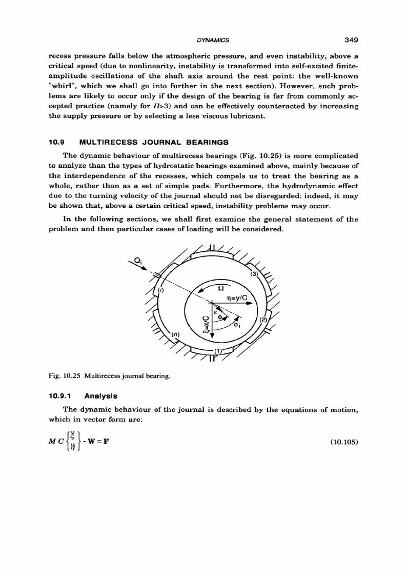
8/9/2019 Hydrostatic Lubrication 1992
http://slidepdf.com/reader/full/hydrostatic-lubrication-1992 366/558
DYNAMICS 349
recess pressure falls below the atmospheric pressure, and even instability, above a
critical speed (due to nonlinearity, instability is transformed into self-excited finite-
amplitude oscillations of the shaft axis around the rest point: the well-known
"whirl", which we shall go into further in the next section). However, such prob-
lems are likely t o occur only if the design
of
the bearing is far from commonly ac-
cepted practice (namely for n>3) nd can be effectively counteracted by increasing
the supply pressure o r by selecting a less viscous lubricant.
10.9 MULTIRECESS JOURNAL BEARINGS
The dynamic behaviour of multirecess bearings (Fig.
10.25)
is more complicated
t o analyze than the types of hydrostatic bearings examined above, mainly because of
the interdependence of the recesses, which compels us to treat the bearing as a
whole, rather than as a set of simple pads. Furthermore, the hydrodynamic effect
due to the turning velocity of the journal should not be disregarded: indeed, i t may
be shown that , above a certain critical speed, instability problems may occur.
In the following sections, we shall first examine the general statement of the
problem and then particular cases of loading will be considered.
Fig.
10.25
Multirecess journal
bearing.
10.9.1
Analys is
The dynamic behaviour of the journal i s described by the equations of motion,
which in vector form are:
M C
f
} - W = F
(10.105)

8/9/2019 Hydrostatic Lubrication 1992
http://slidepdf.com/reader/full/hydrostatic-lubrication-1992 367/558
350
HYDROSTATIC LUBRICATION
where F s the external force and
W
s the resultant of the lubricant pressure on the
journal.
The pressure distribution can be found by solving the Reynolds equation,
namely Eqn 4.18, by numerical computing. In section 8.2
it
has already been pointed
out that, thanks
to
the linearity of the Reynolds equation in the absence of cavitation,
it s solution can be obtained as the superposition
of
n+2 pressure fields, which are
proportional to the
n
recess pressures p i , to & and to
4
-n/2, respectively. The same
may be done for the boundary flow rates. By integrating the pressure fields, we find
that, for any given displacement, the load capacity is
a
linear function of the recess
pressures and of the shaft velocities:
(10.106)
The components of the array
p
are the n recess pressures. The 2xn coefficients Aij
are the contributions of the i-th recess pressure to the load capacity along
5
and q ;
they are functions of the displacement of the journal, although, when small dis-
placements are involved, they may be considered t o be constants.
In order to study small displacements around any steady-state equilibrium
point ( C ~ , $ ~ ) = ( ~ ~ , ~ J ,convenient procedure is to linearize Eqn 10.106, that leads
t o
write the perturbation of load capacity as:
(10.107)
Note th at we have omitted the subscript 's' n the last equation, but it goes without
saying that all the finite parameters are calculated in the equilibrium point; the
same will be done for all the following linearized equations. In Eqn 10.107, the sec-
ond term on the right-hand side accounts for the squeezing effect of lubricant on the
bearing lands (it is analogous to coefficient
B
of pad bearings);
it
is often much
smaller than the first term and may be disregarded, unless recesses are small, or
compressibility is high. The transformation matrix X is defined by the equation
The
2x2
matrix Uw ccounts for the changes of the hydrodynamic load capacity due
to the shaft displacements; in practice, its elements may be obtained by means of
repeated numerical computing, namely considering how much the components of
the hydrodynamic load capacity vary after small displacements S{ and tiq from the
equilibrium point.
A
further term (calculated in the same way) could be added to the
8/9/2019 Hydrostatic Lubrication 1992
http://slidepdf.com/reader/full/hydrostatic-lubrication-1992 368/558
DYNAMICS 351
right-hand side of Eqn 10.107 t o account for the fact that the elements of A are not
exactly constants.
The variations in recess pressure 6pi can be calculated by introducing the con-
tinuity of flow in and out of each recess. The flow rate reaching the lands from each
recess may be obtained (by numerical computing o r other approximate calculations)
as a linear combination of the recess pressures and of the shaft velocities. The flow
rate Qi delivered by the supply system to each recess must be equal to the flow rate
entering the bearing clearance, except for the variation in the density of the lubri-
cant and the variation in the volume of the recess due to the displacement of the
journal; sometimes the variation in volume of the supply pipes (due to the change in
pressure) should also be considered. In other words it may be written as follows (see
also section
10.4):
(
10.108)
In the equation above, A,.i is the area of each recess (we have assumed that all re-
cesses are equal). "Lubricant stiffness" K d is defined as
where
V,
is the volume of a recess,
V,
the volume of the relevant supply ducts and
Kl, the equivalent bulk modulus of the lubricant. In the large majority of cases
Kd
may be considered as a constant.
The components of vector V are the rates of change in each recess volume and
clearly depend on the speed of the journal axis; in the case of equal recesses we
have:
(see Eqn 10.103for the meaning
of
$).
Equations 10.108 may be linearized, after which the variations in the n recess
flow rates may be written in the form
(10.109)
(as for Eqn 10.107, the coefficients of the nx2 matrices q (k ) may be obtained by means
of numerical computing). On the other hand, the flow rates Qi delivered by the

8/9/2019 Hydrostatic Lubrication 1992
http://slidepdf.com/reader/full/hydrostatic-lubrication-1992 369/558
352 HYDROSTATIC LUERICATION
supply system depend on the recess pressures pi, the relationship being connected
with the type of supply system; linearizing, we have:
s&=-Ct6p
(10.110)
For a constant-flow system
we
clearly have ac=O,while for capillary compensation
(see Eqn 10.26) we have:
(10.111)
More complicated statements can be obtained for other supply devices, in particular
in connection with controlled restrictors.
Introducing Eqns
10.110
into Eqns
10.109
and Laplace-transforming, we obtain
where:
AA
Kd
A
= q +
a + - I s
(10.112)
(10.113)
That is, we may obtain a set of n complex equations which establish a relationship
between journal displacements and variations in the recess pressures. We may now
left-multiply Eqn 10.112 by A-1 and substitute it to Sp in Eqn 10.107, in order
to
obtain
the components of the load capacity in the following form:
(10.114)
(it is worth noting that in general the 2x2 matrices K and B depend on the complex
variable
s
except when
A
is real, that is when lubricant compressibility is negligi-
ble). Finally, the equations of motion (Eqns 10.105) become:
( M I s2 + B + K)
= SF(s)
(10.115)
In spite of the formal simplicity of Eqns 10.115, their coefficients would quite
difficult and tedious t o obtain and, since they depend on too many parameters, they
would need to be calculated case by case. In practice, however, great simplifications
may be introduced, especially when particular cases are considered such as, say,
f2=0 or ~ ~ ' 0 .urthermore, the coefficients may be calculated by means of some
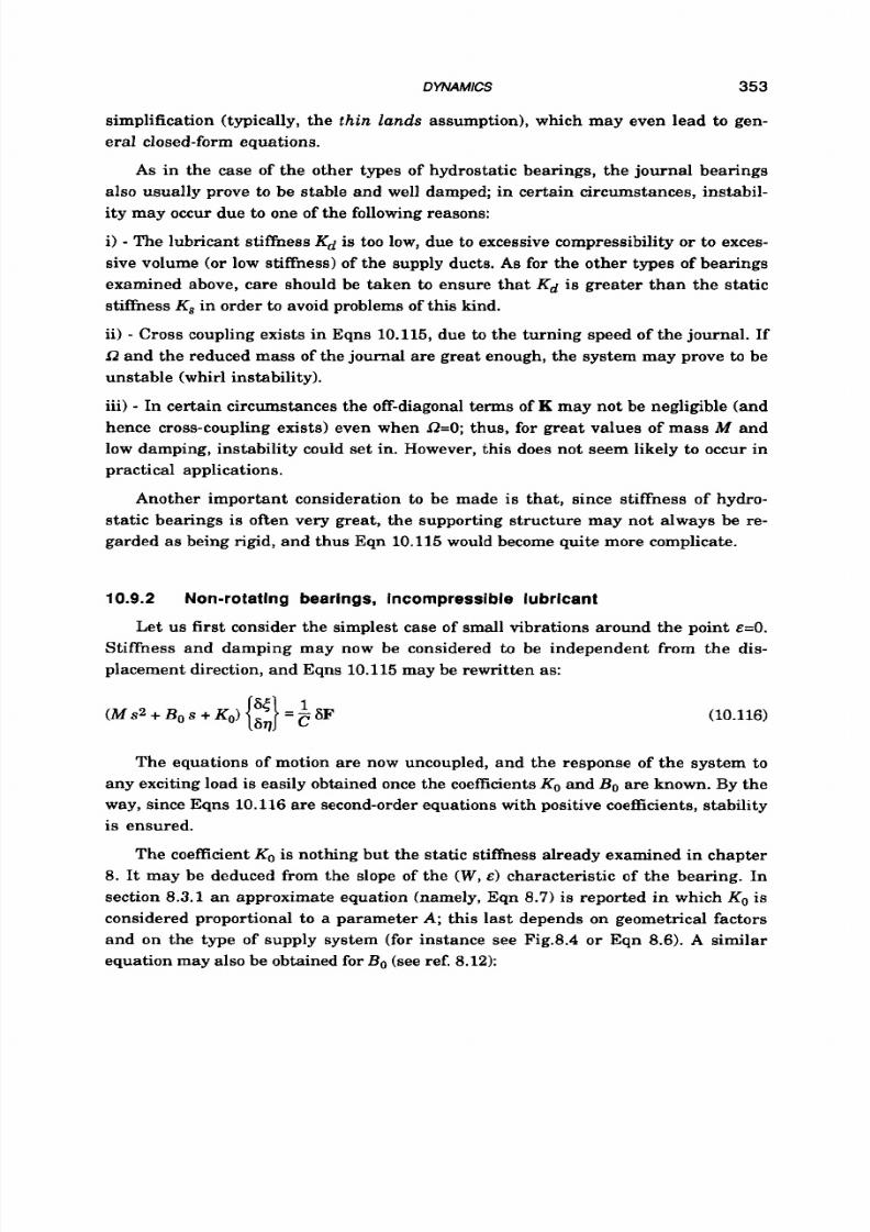
8/9/2019 Hydrostatic Lubrication 1992
http://slidepdf.com/reader/full/hydrostatic-lubrication-1992 370/558
DYNAMICS
353
simplification (typically, the
thin
lands assumption), which may even lead to gen-
eral closed-form equations.
A s in the case of the other types of hydrostatic bearings, the journal bearings
also usually prove to be stable and well damped; in certain circumstances, instabil-
ity may occur due to one of the following reasons:
i)
-
The lubricant stiffness Kd is too low, due to excessive compressibility
or
to exces-
sive volume (or low stiffness) of the supply ducts. As for the other types of bearings
examined above, care should be taken to ensure that
Kd
is greater than the static
stiffness
K,
in order to avoid problems of this kind.
ii) - Cross coupling exists in Eqns 10.115, due to the turning speed of the journal. If
f2 and the reduced mass of the journal are great enough, the system may prove
to
be
unstable (whirl instability).
iii)
-
In certain circumstances the off-diagonal terms of K may not be negligible (and
hence cross-coupling exists) even when Q=O; thus, for great values of mass M and
low damping, instability could set in. However, this does not seem likely to occur in
practical applications.
Another important consideration to be made is that, since stiffness of hydro-
static bearings is often very great, the supporting structure may not always be re-
garded
as
being rigid, and thus Eqn
10.115
would become quite more complicate.
10.9.2 Non-rotat ing bearings, incom pressib le lubr icant
Let us first consider the simplest case of small vibrations around the point E=O.
Stiffness and damping may now be considered to be independent from the dis-
placement direction, and Eqns 10.115may be rewritten as:
(10.116)
The equations of motion are now uncoupled, and the response of the system to
any exciting load is easily obtained once the coefficients
K O
and
Bo
are known. By the
way, since Eqns 10.116are second-order equations with positive coefficients, stability
is ensured.
The coefficient KO is nothing but the static stiffness already examined in chapter
8.
It may be deduced from the slope of the
(W,
) characteristic of the bearing. In
section 8.3.1 an approximate equation (namely, Eqn
8.7)
is reported in which
KO
s
considered proportional to
a
parameter
A;
this last depends on geometrical factors
and on the type of supply system (for instance see Fig.8.4
o r
Eqn
8.6).
A similar
equation may also be obtained for
Bo
(see ref. 8.12):

8/9/2019 Hydrostatic Lubrication 1992
http://slidepdf.com/reader/full/hydrostatic-lubrication-1992 371/558
354
D
L3
B o = 1 2 p ~ u ' ( 1u ' ) 2 A
HYDROSTATIC 1 BRlCATlON
(10.117)
A slightly different equation may be drawn from ref. 8.11.
Even when a static load is applied, Eqns 10.115 may be considered to be uncou-
pled (the off-diagonal terms of the K and B matrices are small). In chapter 8 it has
been shown tha t the a ttitude angle
I$
often has only a small influence on the perfor-
mance of the bearing; hence it is an acceptable loss of generality to take &=O (i.e.
{a ). Several plots of the coefficients
B
and
K
are given in figures from 10.26 t o 10.28
taken from ref. 10.10 and ref. 10.11.
1
a -
0.8
0.6
K
L DPJC
0.4
0.2
0
0
Q2
04 0.6 0.8 1
B
0 8
0.6
B
3&4
L (
D/CP
0.4
0.2
0
-b -
o a2
04
0.6 0.8
I
B
Fig. 10.26 Multirecess journal bearings: stiffness and damping versus the pressure ratio
(n=4,
a'=0.2,
8=36",
L/D=l).
10.9.3
Rotat ing bear ing, incompressible lubr icant
When the journal rotates at high speed, a hydrodynamic load capacity is added
to the hydrostatic one; the sum is clearly intended in the vectorial mode, because the
direction of the resultant of the hydrostatic pressure is close to the direction of the
journal displacement, while the hydrodynamic load capacity is in practice orthogo-
nal to it.
Limiting ourselves to the simplest case of vibrations around
E=O
and incom-
pressible lubricant, Eqns 10.116 can be completed as follows:

8/9/2019 Hydrostatic Lubrication 1992
http://slidepdf.com/reader/full/hydrostatic-lubrication-1992 372/558
DYNAMICS
355
LD:/C/ 0.8
0.4
-b-
1.6
I
- a -
~
Es= 0
-wF
/
0 0.5 1 1.5 2 2.5 0 0.5 1 1.5 2 2.5
L
D
-
L
D
-
Fig. 10.27 Multirecess journal bearings: stiffness and damping versus LID (n=4, '=0.2, 8=36",
J=0.6).
0.8
K
L Dps C
0.6
0.4
0.2
0
2
1.5
B
3pL(D/C13
~-
1
0.5
0
02
0.4
0.6
0.8 1
E s
0
0.2
0.4 0.6 0.8 1
6 s
Fig. 10.28 Multirecess journal bearings: stiffness and damping versus eccentr icity, for various a
( 1 ~ 4 .
=na', ID=l , =0.6).
(10.118)
The coefficient
Ku
s proportional to the rotating speed
R
and needs to be calculated
by numerical means, or on the basis of suitable simplifying assumptions. A n ap-
proximate evaluation is given in ref. 8.11 and ref. 8.12, in which it is found that:

8/9/2019 Hydrostatic Lubrication 1992
http://slidepdf.com/reader/full/hydrostatic-lubrication-1992 373/558
356
HYDROSTATIC LUBR/CAT/ON
(10.119)
Examination of the characteristic equation of the differential system of Eqns
10.118, shows that instability arises when
K,
reaches the critical value
where w, and rare the undamped natural frequency of the shaft and a damping
factor, respectively (Eqns 10.901.
A t the critical speed, corresponding to K,*, the shaft oscillates in an undamped
mode a t the natural frequency
0
(whirl instability). From Eqn 10.119 follows that
the critical speed is:
l 2 * = 2 %
(10.121)
This confirms the well-known fact that, when the turning speed goes beyond the
critical value, the shaft oscillates at a frequency equal to half the critical turning
speed (ref. 10.12).
Equations 10.118 may be used also when the static load is not null, on condition
th at the maximum displacement is small enough (~<0.5) . or a better approxima-
tion we must return
t o
the general form of Eqns 10.115 and calculate the four stiff-
ness coefficients (tha t is the elements of matrix K) nd the four damping coefficients
(matrix
B)
or given values of static displacement kS, and turning velocity a.
simple approximate way is the thin land assumption, that is to assume that, when
land width is small and eccentricity is not great, pressure variation over the lands
is linear (ref. 10.13). Axial and circumferential lands may be treated separately and
flow calculations may be performed using the simple Poiseuille and Couette flow
equations. In practice, the lumped resistance method (see section 8.2) has been
extended to account for turning velocity and for the additional flow rates caused by
the shaft movements around its static equilibrium position (the squeeze effect of the
lands is disregarded, since it is negligible when lands are narrow and fluid is
incompressible). Once the force W due to the pressure of the lubricant has been ob-
tained as a function of the displacement and of the shaft velocity, the dynamic coef-
ficients can be calculated by differentiating the components W, nd Wy ith respect
tox,y,x andy.
A more general approach is based on the numerical solution of the Reynolds
equation, which also allows us to account for possible effects of cavitation (see, for
instance, ref. 10.14, 10.15, 10.16).
Equations 10.118 also allow us t o foresee the dynamic response of the bearing to
external actions. In particular, let us examine the classical case of a harmonic ex-

8/9/2019 Hydrostatic Lubrication 1992
http://slidepdf.com/reader/full/hydrostatic-lubrication-1992 374/558
DYNAMICS
357
citing force of a given angular frequency
o.
aking W,=O (since for small eccentric-
ities the influence of the load angle
is
negligible, there is no loss of generality), Eqns
10.118give:
We may now substitute iw for s, obtaining two complex numbers, whose moduli
and arguments give the amplitude and phase of the oscillation in the 5 and q direc-
tions. The shaft axis is seen to cover an elliptical orbit, the maximum displace-
ments in the
5
and
17
directions being:
I" =& l-w2/w;4 16 ( a 2 - w 2 / w ;2 + 8 c2
1-w2/o;
)2 (R'2+~2 /o :
ISF I
(1-02/w,2
2
+ 4 o /O,
(10.122)
16F I 4 pa2
'" =
[ l-02/c$4 16
c4
( R r 2 - 0 2 / o i2 + 8
(1-w2/02
2 (R.2+q2/o$
in which
R'
is the ratio of the actual turning speed to the critical one:
Examination of Eqns 10.122 mmediately leads to a number of considerations.
First,
the vibration amplitude in the normal direction, with respect to the load, van-
ishes for non-rotating bearings. Actually, this is due to our simplified approach,
since a certain cross-coupling generally exists (namely,
B
and K n Eqns 10.115 are
not diagonal matrices even when a=O,although off-diagonal terms are often quite
small). Then it is easy t o see that the amplitude of vibration becomes infinite when
eu,, nd a=R*,which agrees with the above remarks concerning stability limits.
If we now plot the dynamic flexibility
as
a function of the exciting frequency for
a given value of the damping coefficient, and certain values of the turning speed
(Fig. 10.29),we see that, at high values of R', the hydrodynamic effect makes a con-
siderable (indeed dominant) contribution to the static load capacity. On the other
hand, the damping progressively decreases: at low speed we get an overdamped
behaviour, then a resonant peak occurs, whose amplitude increases, until it be-
comes infinite a t
S'=1.
In conclusion, we see that whirl instability requires particular care during the
design stage, since the actual behaviour of the bearing might prove to be vastly dif-

8/9/2019 Hydrostatic Lubrication 1992
http://slidepdf.com/reader/full/hydrostatic-lubrication-1992 375/558
358 HYDROSTATIC LUBRICATION
- a -
0.0
0.5 1
o 1.5
w
Wn
0.0 05
1 o
1.5
Wn
0
-
Fig. 10.29 Multirecess journal bearings: typical frequency response for various turning speeds
(
c=a.
ferent from what foreseen when the turning speed was not taken into consideration.
Fortunately, however, in most cases, the turning speed in actual applications is far
from dangerous limits.
10.9.4
Compressib le
lubricant
Let us consider a four-recess bearing, rotating at low speed; if the axis of the
journal is assumed to undergo small vibrations along the
z
axis, directed toward
the centre of a recess, the pressure in the side recesses may be considered
t o
remain
practically constant. In this case, a simplified approach may be attempted and the
bearing may be studied just like an opposed-pad bearing. Even, i t is easy to consider
particular types of compensating devices, such as diaphragm-controlled flow di-
viders (ref.
10.4).
A more general approach is delineated in ref. 10.17. The main simplifications
introduced in that work consist in assuming that eccentricity is not too high ( ~ < 0 .5 ) ,
in order
t o
avoid cavitation and large attitude angles, and that, when a harmonic
dynamic load is superimposed
to
the steady load, the journal centre executes plane
small-amplitude harmonic vibration around its steady state position, namely
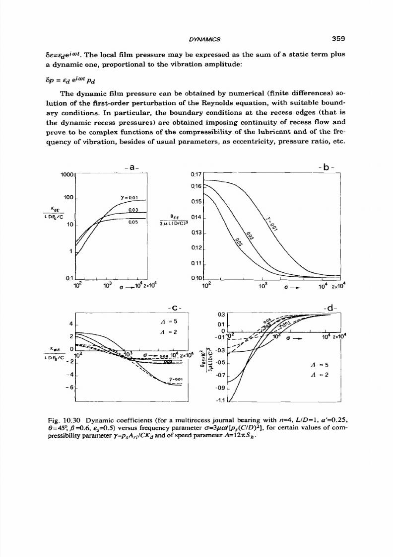
8/9/2019 Hydrostatic Lubrication 1992
http://slidepdf.com/reader/full/hydrostatic-lubrication-1992 376/558
DYNAMICS
359
G&=QeiWt.The local film pressure may be expressed as the s u m of a static term plus
a dynamic one, proportional to the vibration amplitude:
The dynamic film pressure can be obtained by numerical (finite differences)
so-
lution of the first-order perturbation of the Reynolds equation, with suitable bound-
ary conditions. In particular, the boundary conditions at the recess edges (that is
the dynamic recess pressures) are obtained imposing continuity
of
recess flow and
prove to be complex functions of the compressibility of the lubricant and of the fre-
quency of vibration, besides
of
usual parameters, as eccentricity, pressure ratio, etc.
K0.5
LDPslC
- a -
- C -
4 I
-
A
- 2
I
- b -
0.17
J
*lo4
10’ l o3 u - l o 4 2 x ~ 0 4
-d-
A = 5
A
= 2
Fig.
10.30
Dynamic coefficients (for a multirecess journal bearing with r r 4 ,
L / D = l , a ‘ = 0 .2 5 ,
0=45q
J
.6,
~ ~ 4 . 5 )ersus frequency parameter
a=3ptw’[pS(CID)z] ,or
certain values of com-
pressibility parameter
y=psAri /CK,
and of speed parameter
.4=12xSh.
8/9/2019 Hydrostatic Lubrication 1992
http://slidepdf.com/reader/full/hydrostatic-lubrication-1992 377/558
360 HYDROSTATIC LUBRICATION
By integration of the dynamic pressure field acting on the journal we can obtain
the radial and tangential components of the dynamic load and, hence, the relevant
stiffness and damping coefficients:
K , + i w B ,
K4&+ i
w
Be
Obviously, the four coefficients ar e functions of the frequency of vibration and
also depend on the geometrical parameters, on eccentricity, on lubricant compress-
ibility and on pressure
ratio;
moreover the cross coefficients
K@&
nd
B @
depend on
angular speed, too, whereas the direct coefficients are practically not affected by
0.
A
lot of calculations are therefore required in order to give a full description of the
dynamic characteristics of
a
bearing with given geometrical ratios: in ref. 10.17, for
instance, the calculations of the coefficients for a typical bearing a re condensed in
several plots, some of which are shown in Fig. 10.30.
REFERENCES
10.1
10.2
10.3
10.4
10.6
10.6
10.7
10.8
10.9
Opitz H., Bottcher R., Effenberger W.;
Znuestigation on the Dynamic Be-
hauiour of Hydrostatic Spindle-Bearing Systems;
10th
Int. MTDR Conf., Uni-
versity of Manchester, 1969, pap.
MS-21;
15pp.
Masuko M., Nakahara T.; The Influences o f th e Fluid Capacitance in the Oil
Feed Li ne S yste m on the Transient Response of Hydrostatic G uideways;
Int.
J .
Mach. Tool Des. Res.,
14
(19741,233-244.
Wilcock D.
F.; Externally Pressurized Bearings as Servomechanisms. - The
Simple Thrust Bearing; ASME Trans., J . of Lubrication Technology, 89
(1967),418-4 24.
Chen K. N., Yang G. P., Wang
X.,
Yang H. H.; A System Approach to the
Dynamic Characteristics of Hydrostatic Bearings Used on Machine Tools;
Int. J. Mach. Tool Des.
Res.,
20 (19801, 287-297.
Prabhu T. J., Ganesan
N.;
Characteristics of Conical Hydrostatic Thrust
Bearings under Rotation;
Wear, 73 (1981),95-120.
Moshin M. E., Morsi S. A.;
The Dynamic Stiffness of Controlled Hydrostatic
Bearings; ASME Trans., J . of Lubrication Technology,
91
(19691, 597-608.
Wylie C. R., Barrett L. C.;
Advanced Engineering Mathematics;
MacGraw
&
Hill, 1985; 1103 pp.
Ogata
K.; Modern Control Engineering;
Prentice-Hall, 1970; 836 pp.
Inasaki I.; Stability o f Hydrostatic Journal Bearings; Eurotrib 81, proc.
3rd
Int. Tribology Congr., Warszawa, 1981, vol.
2;
pp. 116-122.
10.10
Ghosh
M.
K.;
Dynamic Characteristics of Multirecess Externally Pressurized
Oil Journal Bearing; ASME Trans., J. of Lubrication Technology, 100 1978),
467-471.

8/9/2019 Hydrostatic Lubrication 1992
http://slidepdf.com/reader/full/hydrostatic-lubrication-1992 378/558
DYNAMICS 361
10.11 Ghosh M . K., Majumdar B. C.; Stiffness and Damping Characteristics of
Hydrostatic Multirecess Oil Journal Bearings; Int.
J .
Mach. Tool Des. Res.,
18 (19781,139-151.
10.12 Leonard R., Rowe
W . B.; Dynamic Force Coefficients and the Mechanism of
Znstability i n Hydrostatic Journal Bearings;
Wear,
23
(19731,277-282.
10.13 Vermeulen M., e Shepper M.; Theoretical and Experimental St ud y of the
Dynamic Behaviour
of
Hydrostatic Radial Bearings;
Eurotrib 89,
proc.
5th Int.
Congr. on Tribology, Helsinki, 1989, vol. 3;p. 180-185.
10.14 Chen
Y.
S.,Wu H. Y., Xie P. L.; Stability of Multirecess Hybrid Operating O il
Journal Bearings;
ASME Trans.,
J. of
Tribology, 107 (19851,115-121.
10.16 Rowe W. B., Chong F.
S.;
Com putatio n of D ynam ic Force C oefficients for
Hybrid (Hydrostatic JHydrodyn amic) Journal B earings by th e Finite D istu r-
bance and Perturbation Techniques; Tribology International, 19 (19861, 260-
271.
10.16 Lund
J.
W.;
Review
of
the
Concept of Dynamic Coefficients for F luid Fil m
Journal Bearings;
ASME Trans.,J.
of
Tribology, 109 (19871,37-41.
10.17 Ghosh M.
K.,
Viswanath
N. S.; Recess Volume Fluid Compressibility Effect
on th e Dynamic Characteristics of Multirecess Hydrostatic Jou rna l Bearings
w ith Journal Rotation;
ASME Trans.,J. of Tribology, 109 (19871, 417-426.
8/9/2019 Hydrostatic Lubrication 1992
http://slidepdf.com/reader/full/hydrostatic-lubrication-1992 379/558
Chapter
11
OPTIMIZATION
11.1
INTRODUCTION
In this chapter an important aspect of the study and design of hydrostatic bear-
ings, already presented in previous chapters, especially in chapter 6, will be dealt
with. The "optimum" conditions corresponding to the minimum power dissipated
by the bearing will be identified and a general procedure for the solution of the prob-
lem will be described.
Our investigation is carried out on an infinitely long pad directly supplied by a
pump. The same procedure
is
then applied t o real bearings. Afterwards, the inves-
tigation is extended to an infinitely long pad and real bearings supplied by means of
compensators. The results will also show that a direct supply system, as compared
with a compensated supply system is more efficient (that is, less power is dissipated
and stiffness is greater).
This subject may be dealt with using only some of the elementary formulae of
hydrostatic lubrication presented in chapters
4
and 5 .
11.2
GENERAL PROCEDURE
First of all we shall s tart with the study of the static behaviour of an elementary
hydrostatic bearing: the infinitely long hydrostatic pad, Fig. 11.1,
of
which we shall
consider a finite part and afterwards we shall go on t o determine its optimum
dimensions.

8/9/2019 Hydrostatic Lubrication 1992
http://slidepdf.com/reader/full/hydrostatic-lubrication-1992 380/558
OPTlMIZ4TlON 363
The pad is
first
considered as being supplied directly (Fig. 1l .l .a) and then as
being supplied by a compensating element (Fig. ll .l .b), and in both cases first when
the pad is still and then when
it
is in motion.
Therefore, we shall start with a pad that is supplied directly and still. Consider-
- a -
- b -
Fig. 1 1 . 1 Hydrostatic pad of infinite length. A finite length L
of
it
is
considered. a- Direct supply;
b- Compensated supply (supply
through
compensating elements).

8/9/2019 Hydrostatic Lubrication 1992
http://slidepdf.com/reader/full/hydrostatic-lubrication-1992 381/558
364
HYDROSTATIC LUBRICATION
ing tha t its behaviour is described by the fundamental flow rate-pressure relation,
Eqn 4.48, we assume that:
the lubricant
flow
rate Q is constant; we then verify the variation of recess
pressure p r and of the other quantities: load capacity
W,
stiffness K and dis-
sipated pumping power H p , as functions of the characteristic variables:
length L , recess width b, film thickness h , and lubricant viscosity p ; the pad
width B is generally assigned.
Afterwards we assume that:
recess pressure
p,. is
constant; starting from
Q
we continue as above.
Finally, we assume that:
load
W is
constant and we continue as above.
It
should be noted that al-
though W is a derived quantity it is fundamental for the determination of the
dimensions of any hydrostatic system, as it is almost always assigned and
often the most important required characteristic.
In the investigation described above, particular care is taken in the determina-
tion of the constrained minima of H p , that is of the corresponding optimum values
o f L , b , h and
p ,
considered individually.
Afterwards a moving pad is considered. Its performance
is
described by the
fundamental relation Eqn
4.49,
and, assuming that speed
U
s
constant, the varia-
tions of friction F, of dissipated friction power H f and of friction coeficient f as func-
tions of L,
b, h,
and p , are verified.
Finally the variation of the total dissipated power H,, that is the s u m of H p and
H f , is considered and its minima and the corresponding optimum values of
L,
b , h ,
and
p
in the three above-mentioned cases are determined: Q constant,
pr
constant,
W
constant and assuming in all cases that
U
s constant. Optimization is first car-
ried out as regards one variable, then two, three and finally all four variables. The
concept of pad emciency is also introduced.
The optimization procedures obtained for the infinite pad, that are already in-
dicative for any real pad, are transferred in the end to specific pads: the rectangu-
lar, the circular and the annular pads.
Afterwards the pad supplied by means of
a
capillary tube is considered. In such
a case the ratio
/3 (Eqn
5.15)
between recess pressure
p r
and supply pressure p s also
plays
a
role. As done before, the pad is first studied when
it
is still and assuming
that there is
a constant supply pressure
p s
and then
a constant load
W.
In both cases
p
is obviously taken into account.
Afterwards the moving pad is studied.
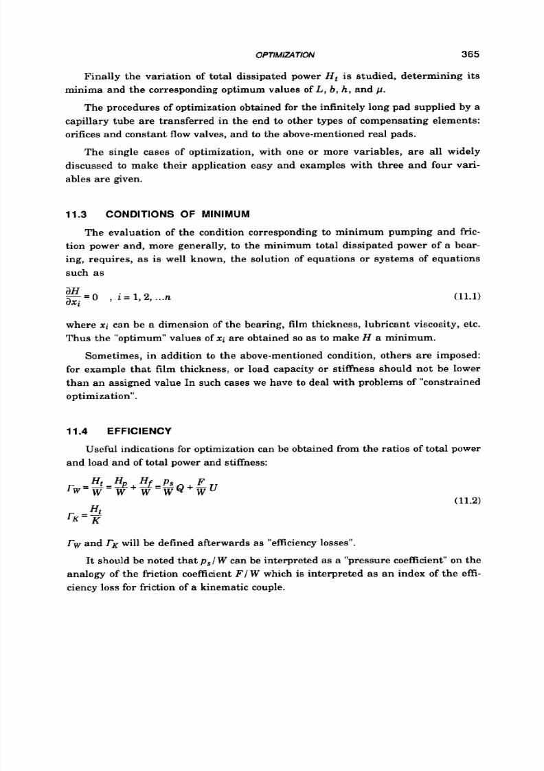
8/9/2019 Hydrostatic Lubrication 1992
http://slidepdf.com/reader/full/hydrostatic-lubrication-1992 382/558
OPTlMlZATlON
365
Finally the variation of total dissipated power H t is studied, determining its
minima and the corresponding optimum values of
L, b, h,
and
p .
The procedures of optimization obtained for the infinitely long pad supplied by a
capillary tube are transferred in the end to other types of compensating elements:
orifices and constant flow valves, and to the above-mentioned real pads.
The single cases of optimization, with one
or
more variables, are all widely
discussed to make their application easy and examples with three and four vari-
ables are given.
11.3 CONDITIONS OF MINIMUM
The evaluation of the condition corresponding to minimum pumping and fric-
tion power and, more generally, t o the minimum total dissipated power of a bear-
ing, requires, as is well known, the solution of equations o r systems of equations
such as
0
,
i = 1, 2,
...
n
H
a x i
-=
(11.1)
where
x i
can be a dimension of the bearing, film thickness, lubricant viscosity, etc.
Thus the "optimum" values
of
xi are obtained so as to make
H
a minimum.
Sometimes, in addition
t o
the above-mentioned condition, others are imposed:
for example that film thickness, or load capacity or stiffness should not be lower
than an assigned value In such cases we have
t o
deal with problems of "constrained
optimization".
11.4 EFFICIENCY
Useful indications for optimization can be obtained from the ratios of total power
and load and
of
total power and stiffness:
(11.2)
r w and
r,
will be defined afterwards as "efficiency losses".
It should be noted that psl W can be interpreted as a "pressure coefficient" o n the
analogy of the friction coefficient
F l
W
which is interpreted as an index
of
the em-
ciency loss for friction of a kinematic couple.
8/9/2019 Hydrostatic Lubrication 1992
http://slidepdf.com/reader/full/hydrostatic-lubrication-1992 383/558
366
HYDROSTATIC LUBRICATIOW
11.5
DIRECT SUPPLY
Let us consider the infinitely long pad in Fig. l l . l . c ,of width B , directly supplied
by a pump (Fig. 5.11.a),and let us study the performance of a portion
of
length L.
11.5.1 Steady pad
11.5.1.1
Given
flow rate. Flow rate Q is assumed to be constant. This is easily ac-
complished in the case of direct supply with a constant flow supply pump. Film
pressure which is determined using Eqn 4.46, replacing z with x, considering Eqn
4.48 and disregarding the sign of absolute value, is
while recess pressure is
1
B - b
~r = 3~
Q 7
If the losses in the
supply pressure p s . In
(11.3)
supply line are assumed to be equal to zero, p r equals the
this chapter the notation p r = R Q , where R is the hydraulic
resistance of the bearing (section
4.7.21,
will be rarely used, whereas, in previous
chapters, i t was used for the sake of synthesis. The diagram of the recess and film
pressures of the bearing is showing in Fig. 11.1.~.
The dissipated pumping power
H p ,
given by Eqn 5.3, with p s = p r ,
is
1
B - b
H p = 3p
Q 2
-
h3
L
Load capacity
W,
3 1
W = p Q
p B2 b2)
(11.4)
obtained from Eqn 4.47 with Eqn 11.3,is
(11.51
Therefore stiffness
K,
given by Eqn
5.8,
is
(11.6)
Let
us
now consider the influence
of
the dimensions
of
the bearing, t ha t is its
length L, idth
B
and recess width b, on the above-mentioned quantities and then
on the performance of the bearing. Using B as the “reference“ dimension we
introduce
L
L ’ = B
(11.7)
8/9/2019 Hydrostatic Lubrication 1992
http://slidepdf.com/reader/full/hydrostatic-lubrication-1992 384/558
OPTIMIDITION
367
and so pressure p r may be expressed as a dimensionless function of
L'
where
p,.o=pQ(B-b)
Bh3
is the reference pressure. Pumping power
H p
becomes
(11.8)
(11.9)
where Hpo*=pQ2(B-b) /Bh3 s the reference power. It should be noted that H i = p ; .
Such equalities between dimensionless quantities will often be found from here on.
In Fig. 11.2.a
p ;
and
H i
are presented as functions of
L' .
They are inversely propor-
tional t o L'.
Introducing
b
b ' = B
the following dimensionless functions of b' are obtained:
3
p ; = H i = 3 ( 1 - b ' ) ,
W'
= = (1 b'2)
(11.10)
(11.11)
In Fig. 11.2.b W',
K ,
; ,
H i
are presented. They decrease as
b'
increases.
Let us now consider the influence of film thickness expressed in the usual
dimensionless form
h ' = -
h0
(11.12)
where ho is the reference film thickness. The following relationships are obtained:
(11.13)
In Fig. 11.2.c W',
K ' , p ;
and H i are given. They decrease rapidly as h' in-
creases. These diagrams show the performance of the bearing working with vary-
ing loads. It should be noted that, as film thickness reaches zero, the bearing would
bear infinite loads (with infinite stiffness). This is obviously not possible, since the
pump should yield an infinite pressure and the supply system should bear it: in
practice the maximum pressure is limited by a relief-valve placed downstream
from the pump (Fig. 1l.l .a).
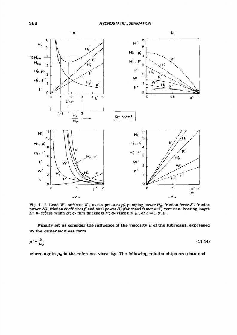
8/9/2019 Hydrostatic Lubrication 1992
http://slidepdf.com/reader/full/hydrostatic-lubrication-1992 385/558
360 HYDROSTATIC LUBRICATION
12
10
8
6
4
2
0
H i
Hb. ~ ' r
Hi, F'
1'
W '
K '
- a -
6
5
4
4, P
4
H i , F '
3
2
1
0
f '
W '
K '
0
L'opt
x
/3
1
H
3
- -
HD
0 1 h'
- c -
- b -
0
0.5
b'
6
5
4
3
2
I
H;
H9
Pr
H i , F'
W '
K'
a
0
- d -
Fig.
11.2
Load
W ,
stiffness K , recess pressure
p;,
pumping power H', friction force F', friction
power
H j ,
friction coefficientf' and total power
H ;
(for speed factor k=4) versus:
a-
bearing length
L'; b-
recess width b';c-
film
thickness h';
d-
viscosity p', or c'=(l-b')p'.
Fina l ly le t
us
consider
the
influence of
the
viscosity
p
of
the
lubricant , expressed
in
the d imens ionless form
=
JL (11.14)
PO
w h e r e a g a i n
po
is the
referenc e viscosity. T he following relation ship s
are
obtained
8/9/2019 Hydrostatic Lubrication 1992
http://slidepdf.com/reader/full/hydrostatic-lubrication-1992 386/558
OPTiMiZ4 TION
369
(11.15)
In Fig. 11.2.d W',
K',
i, Hi are presented. They vary linearly with p'. Such
diagrams may be employed
t o
study the performance of the bearing in operating
conditions, as p varies with temperature. So, if viscosity decreases because temper-
ature increases, load also should decrease. Since that is generally impossible in
operating conditions, film thickness must decrease.
11.5.1.2
Given
pressure. Supply pressure
p s
is assumed to be constant; therefore if
there are no friction losses in the supply line, recess pressure
p r = p s
is a l s o constant.
The following formulas ar e especially interesting for the study and design of a bear-
ing operating
at
a given pressure which, for the sake of safety, is generally much
lower than the maximum pressure the pump can supply or the supply circuit can
bear.
Load capacity is given by Eqn 4.47 which may be rewritten as
1
(4.47 rep.)
=
j p r
L ( B + b )
The product L B is the pad area. It is often defined as "projected pad area" to distin-
guish
it
from the product
L[ (B+ b) / 2 ]
efined as the "effective pad area".
Stiffness is
3 P
2 h
= - ' L (B + b )
Flow-rate is
Pumping power is
(11.16)
(4.48 rep.)
(11.17)
In dimensionless form the following expressions, functions of L ' , are obtained:
Figure 11.3.a shows the linear variations of W , K , Q' and H i with L' . Consider-
ing their dependence on
b'
they can be written as:
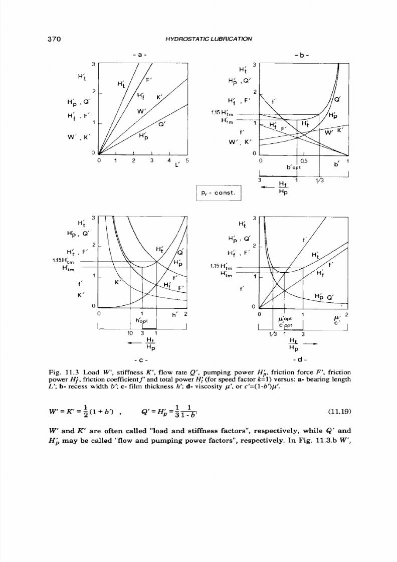
8/9/2019 Hydrostatic Lubrication 1992
http://slidepdf.com/reader/full/hydrostatic-lubrication-1992 387/558
370
HYDROSTATIC LUBRICA TlON
- a -
3
H i
2
H b
, Q '
H i
,
F'
1
W ' ,
K '
0
3
H i
l ib
, Q '
2
H i
,
F '
1.15H;,
~
Hi, __-
I
f '
W ' , K '
0
- b -
7
0 1 2 3 4 5
L'
pr
=
const.
u
P
3
H i
I
Q'
Hi
,
F'
2
1.15H;, ___
Hi, ~-
I
f '
0
10
3
1
-H t
HP
l/s 1
3
h-
"P
- c - - d -
Fig. 11.3 Load W', stiffness
K',
low rate Q', pumping power H i , friction force F', friction
power
Hi ,
friction coefficientf' and total powerH; for speed factor k = l ) versus:
a-
bearing length
15';b- recess width 6'; c- film thickness h';
d-
viscosity p ' , or c'=( 1-6')p'.
1 1 (11.19)
'=H' --
1
w = K ' = 2 ( 1 + b ' ) ,
P
3 1 - 6 '
W'
and
K'
are often called "load and stiffness factors", respectively, while Q ' and
H i may be called "flow and pumping power factors", respectively. In Fig. 11.3.b
W',
8/9/2019 Hydrostatic Lubrication 1992
http://slidepdf.com/reader/full/hydrostatic-lubrication-1992 388/558
OPTlMlzATlON
371
K , Q'
and
H i
are plotted against
b'.
While
W'
and K' vary linearly with
b', Q'
and
H i vary exponentially.
Considering the dependence on
h'
the following expressions are obtained:
(11.20)
In Fig. 11.3.c
K ' ,
Q'
and
H L
are plotted against
h'.
The
first
quantity is inversely
proportional to
h'
while the others increase according to
a
cubic law.
Finally, considering the dependence on
p ' ,
the following expressions are
obtained:
(11.21)
Figure 11.3.d shows the inversely proportional variations of
Q'
and
H i
with
p ' .
11.5.1.3 Given
load.
The load
W
carried by the pad is assumed to be constant and
equal t o an assigned value, as commonly occurs in practical applications and there-
fore in design. Recess pressure is
(11.22)
Stiffness is
(11.23)
K = 3 h
Flow-rate is
Pumping power is
(11.24)
(11.25)
In dimensionless form the following expressions, functions of L', re obtained:
4 1
p;=L' I
H ; = j L ' (11.26)
In
Fig. 11.4
p;
and
H b
are plotted against
L',
with both quantit ies inversely propor-
tional
to
L'.
Considering the dependence on
b
the following expressions a re obtained:

8/9/2019 Hydrostatic Lubrication 1992
http://slidepdf.com/reader/full/hydrostatic-lubrication-1992 389/558
372
HYDROSTATIC
L
UBRlCATlON
- a - -b
-
1
0.8
0.6
b'opt
0.4
0.2
0
bopt
u
2
4 6 8 k 1 0
3
H;
H6
Him-
2
1.15H;,
Hi,
, f
'
1
Q'
K '
C
~
1/5 1 3
--
i
HP
I h' 2
I h'opt 1
- C -
3
/3
1
3
P
- d -
Fig.
11.4
Stiffness K'. recess pressure
p;,
flow rate
Q',
umping power H' friction force
F' ,
friction power
H i ,
friction coefficient
f'
and total power
H ;
(for speed &;tor
k = l )
versus:
a-
bearing length
L',
or
g'=L'p';
b- recess width
b'; c-
film thickness
h';
d- viscosity
p'.
In case
b
optimal recess width
b&
versus speed factor
k is also
represented.
(11.27)
2 1 4 1
Q ' = - -
i== 9
3
1
- b"
'
Hb
=
3
(1 +
b')
(1
- b")
In Fig.
11.4.b
p;,
Q'
andH i are plotted against b':p; decreases,
Q'
increases,
H i
has
a minimum. Such minimum value
is
important
for
the optimization
of a
bearing
8/9/2019 Hydrostatic Lubrication 1992
http://slidepdf.com/reader/full/hydrostatic-lubrication-1992 390/558
OPTlMlzATlOfU 373
and it can be determined by solving Eqn 11.1 for i = l and
x l = b ' ,
thus yielding b'=1/3.
It should be noted tha t around that value Hb is not critical so that greater values of
6' may also be used. The value of 0.5 is often suggested for b', with a n increment of
H i
lower than
6%,
with respect to its minimum value.
Considering the dependence on h ' the following expressions a re obtained:
1
K= r
Q'=3h'3 ,
(11.28)
In Fig. 11.4.c K', Q' and Hi, re plotted against h'. The first quantity is inversely
proportional to h' while the others increase with a cubic law.
Finally, considering the dependence on
p',
the following expressions are
obtained:
(11.29)
Figure 11.3.d shows the inversely proportional variations of Q' and H i with p'
11.5.2
Moving
pad
If the pad shown in Fig. 11.1 should move in the z direction, perpendicular to its
length, the influence
on
it s performance of the inertia forces acting on the lubricant
in the recess as well as the effect of lubricant recirculation in the recess cannot be
disregarded. On the other hand if the pad moves in the direction of its length, the
influence is nil. In this case the expressions relevant t o the motionless pad still hold
good, as well as the following expression of the friction force in the recess.
11.5.2.1
Friction. The friction force in the film is given by Eqn
4.49
F f =
p
U L
( B
b )
(4.49
rep.)
The friction force in the recess is
F f p= p U
1
P
L
B
Friction power is given by Eqn
5.5,
where &O. As regards the power dissipated in
the film, this is
H f Z p i F i L ( B - 6 )
while in the recess it is
(11.30)
8/9/2019 Hydrostatic Lubrication 1992
http://slidepdf.com/reader/full/hydrostatic-lubrication-1992 391/558
374 HYDROSTATIC LUBRICATION
If the recess is not too wide, a s often happens, andfor its height is much greater that
the thickness of the film,
H f p
s negligible compared to
H f ,
as will be assumed from
here on.
The power necessary to accelerate the lubricant in the film should also be added
to I f f , hat is:
However, even for high values of U ,Hl is generally negligible compared to H f , as
will be assumed from here on.
Ff
and
H f
may be expressed as dimensionless functions of
L':
=
L' (11.31)
H H
= L' f=
5
F f
F i . - F f o
- 1U K B ( B - b ) ' Hi- - H f o p u 2 K i ( B - b )
where F f o = p U ( l f h f B ( R - b )nd H f o = p U 2 ( l f h ) B ( R - b )re reference values for the fric-
tion force and power. Figures 11.2.a, 11.3.a and 11.4.a show how F j and H i vary
linearly with
L' .
Considering the dependence of
Ff
and
H f
on
b'
they can be written as:
F j = H i = 1 - b '
(1 .32)
F i
may be called the "friction factor" while
H i
is sometimes called the "power fac-
tor". Figures 11.2.b, 11.3.b and 11.4.b show how
F j
and
H j
decrease linearly as
b'
increases.
Considering the dependence on h' the following expressions are obtained:
1
F j
= H i
= r
(11.33)
Figures 11.2.c, 11.3.c and 11.4.c show the inversely proportional variations of F j and
H j with h' .
Finally, considering the dependence on
p'
the following expressions are
obtained:
F j = H j = p' (11.34)
Figures 11.2.d, 11.3.d and 11.4.d show how
F j
and
H j
vary linearly with p'

8/9/2019 Hydrostatic Lubrication 1992
http://slidepdf.com/reader/full/hydrostatic-lubrication-1992 392/558
OPTIMIZATION
375
11.5.2.2
Friction coefficient.
If the flow rate is assigned and then load capacity is
expressed by Eqn 11.5, the friction coefficientf=Ff lW becomes
2 u
L
3 Q B + b
f
=--
h2
-
If expressed in dimensionless form, as a function of
L' ,
6' and h', i t becomes
(11.35)
(11.36)
In Fig. 11.2.a and Fig. 11.2.b,f is plotted against
L'
and b': its variations are simi-
lar to those of F j and
H i ;
in Fig. 11.2.c, f ' is plotted against h': it s variation differs
from those of F j and H i as i t increases with h'.
If pressure
is
assigned and load capacity
is
given by Eqn 4.47, the friction coefi-
cient is
f = 2 - p - -1 B - b
p r h B + b
(11.37)
When expressed in dimensionless form,
as
a function of b', h' and p', it becomes
(11.38)
In Fig.
11.3.b,
11.3.c and 11.3.d f is plotted against b', h' and p': its variations are
similar to those of
F j
and
H i .
Finally, if load is assigned, f ' may be expressed as
u 1
f
= p
w k
(B - b)
(1
.39)
In dimensionless form, as a function of
L ' ,
b ' , h' and p', it becomes
Figures 11.4.a, 11.4.b, 11.4.c and 11.4.d show how the variations off' are identical to
those of
F i
and H i .
11
25.3
11.5.3.1 Given f low rate. In the case of direct supply and constant flow rate, pad total
dissipated power, given by Eqn 5.6, is obtained by adding Eqn 11.4 to Eqn 11.30, that
is
Minimum dissipated power and ef f ic iency losses
8/9/2019 Hydrostatic Lubrication 1992
http://slidepdf.com/reader/full/hydrostatic-lubrication-1992 393/558
376 HYDROSTATIC
LUBRICA
TION
(11.41)
Introducing a reference pumping power, total power H t may be expressed in
dimensionless form, as
a
function
of
L':
where
U B h
k
=-
Q
k
may be called a "speed parameter".
H i
is
minimum for
d3
LhPt
=
-
k
and for such a value of L' it is
(11.42)
(11.43)
(11.44)
(11.45)
where
H f I H ,
is
the often mentioned "power ratio". Equation
11.45
and Eqn
11.60
below were given for the first time in ref. 2.3 and have been used many times in
optimization problems in previous chapters. In Fig. 11.2.a H i is plotted for k = l .
Within the range 1<HfIHp<3,Hi differs from its minimum by less than 15%.
The speed parameter is related
to the
power ratio by the following equation:
where Hp0*=pQ2(B-b) lh3Bnd Hfo*=pU2B(B-b)Ih.
Considering the dependence on b' ,
HI
can be expressed as
(11.46)
L h
Q
i = 3 ( 1 - b ' ) + k z ( l - b ' ) , with
k = p
In Fig. 11.2.b H i is plotted for k = l . As b' approaches 1 , H i as well as W' and K ap-
proach
0.
H i can be expressed as the following function of h':
1 1 U L h oH ; = 3 7 + k 2 j 7
,
with
k=-
h Q
( 1 .47)
8/9/2019 Hydrostatic Lubrication 1992
http://slidepdf.com/reader/full/hydrostatic-lubrication-1992 394/558
OPTlMlZATION
377
In Fig. 11.2.c Hi is plotted for k = l . A s h' increases, Hi decreases; W' also decreases
but more rapidly and K even more
so.
Finally considering the dependence on p ' the following expressions are
obtained:
Hi = 3 p' + k2 p'
(11.48)
where K is given by the second of Eqns 11.46. In Fig. 11.2.d Hi is plotted for k = l . H i
decreases linearly with
p'
as do W and K'.
A s regards the variation of H't as a function of
B,
considered a reference quan-
tity until now, it is sufficient to put
(11.49)
B ' = b
and we immediately get the variation of
H&B')
from that of Hi(b').
The study of the variation of total dissipated power Ht becomes more complicated
if it is considered as
a
function of two
or
more variables unless they a re
b (or B )
and
p. Indeed, in such a case the following "compound variable can be introduced:
C'=(l-b')p' (11.50)
and Eqn 11.41 becomes
Hi
=
3
C ' + k 2 ~ '
(11.51)
similar to Eqn 11.48 and Eqn 11.46 and wi th the same
k.
In Fig. 11.2.d Hi(c') is also
plotted, for k = l .
10- In the previous paragraphs i t has been shown tha t if b, h, p
(and B ) vary in such a way as to make
H,
decrease,
W
and
K
also decrease though in
a different way;
this
must generally be taken into account in dimensioning a bear-
ing. In this connection useful informations may be obtained from the "efficiency
loss"
rw,r
from its inverse (ref. 9.41, and from
r K
given by Eqns 11.2. Considering
the dependence on b', dividing Eqn 11.46 by the second of Eqns
11.11
gives us:
(11.52)
Both rb and r k decrease as b' approaches 1 suggesting the choice of a wide recess.
In Fig. 11.5.a
rw
and rk are plotted for k=O, 1,2.
Considering the dependence on
h',
dividing Eqn 11.47 by the second and the
third of Eqns 11.13,respectively, gives

8/9/2019 Hydrostatic Lubrication 1992
http://slidepdf.com/reader/full/hydrostatic-lubrication-1992 395/558
378 HYDROSTATIC LUBRICA
TlON
In Fig. 11.5.b Tb(h') and rk(h ' ) re plotted for h=O, 1, 2. riy decreases
as
h' ap-
decreases
as
h'
approaches
0
in every case.
This
roaches 0 except for k=O, while
suggests the choice of a small film thickness.
- a -
- b -
5
4
3
rh
2
1
0
Q
= c ons t .
E l
0.5 b l 1
2
h '
Fig.
11.5 Efficiency losses
rb
and rK ersus:
a-
recess width
b', b-
film thickness
h',
for cer-
tain values of speed factor
k .
Finally from Eqn 11.48 and from the second of Eqns 11.15 it transpires that the
efficiency loss does not depend on lubricant viscosity.
The choice of the values of the variables B, L, 6, h, and p also depends on various
other conditions which may be encountered in the design of a bearing, regarding its
operation and construction. For example, in actual pads, Fig. 6 .25 , it
is
convenient
to choose BSLSZB.
11.5.3.2
Given
pressure. Total dissipated power is
H t , expressed in dimensionless form, as a function of L', is given by:

8/9/2019 Hydrostatic Lubrication 1992
http://slidepdf.com/reader/full/hydrostatic-lubrication-1992 396/558
OPTIMIZATION 379
(11.55)
where k is similar to the Sommerfeld number
of
plane hydrodynamic pads. In Fig.
11.3.a
Hi
is plotted for k = l .
Hi
decreases linearly with L' as well
as W
and
K'.
Considering the dependence on 6 ' )Hi can be expressed as
(11.56)
1 _l .L .E
P r h2
i = 3 1 + 6 ' 2 ( 1 - 6 ' ) , with k -
Hi is minimum for
1 1
6ipt = 1
3
(11.57)
to which Eqn 11.45 still corresponds. It should be noted that Eqn 11.57 leads to 6Apt<0
for k<l/&; in practice
6Apt=0
up
t o
k=1/fi and afterwards it rapidly approaches
unity. In Fig. 11.3.b Hi is plotted for k = l .
H i
can be expressed as the following function of h':
(11.58)
Hi
is minimum for
hApt =6 (11.59)
to which the following relation corresponds:
It should be noted that from Eqn 5.7 high values of the ratio HfIHpcan lead
to
high
temperature increments. In Fig. 11.3.c
Hi
is plotted for
k = l .
Finally considering the dependence on
p '
the following expressions are
obtained:
HI is minimum for
1 1
Pbpt = 3 i
(11.61)
(11.62)
t o which Eqn 11.45 again corresponds. In Fig. 11.3.dH i is plotted for k= l.
8/9/2019 Hydrostatic Lubrication 1992
http://slidepdf.com/reader/full/hydrostatic-lubrication-1992 397/558
380
HYDROSTATIC LUBRICATION
It should be noted that, within the range 1<H+Hp<3, Hi(b') as well as Hi(h') and
H&p') differ from their minima by less than 15%. As regards the variation of H i as
a function of B', given by Eqn 11.49, it can be immediately deduced from that of
Hi(b').
Therefore we may conclude that high values of B' can be used for
k>O,
too.
For example, with reference to Fig. 11.3.b for k = l , putting
B'=- ,
the value of H i
would not exceed its corresponding value for B&l/b~pt=2.37 by more than 15%.
Considering Eqn 11.50, Eqn 11.54 becomes
H i is minimum for
1 1
c b p t = z i
(11.63)
(11.64)
to which Eqn 11.45 again corresponds. In Fig. 11.3.d Hi(c'1, given by Eqn 11.63,
is
also plotted, for k = l . Therefore we can immediately look for the minimum value of
Hi : ckpt is determined from Eqn 11.64 and then any couple of values of
b '
and p'
which satisfy Eqn 11.50 yield such a minimum. The choice of such values makes
the selection of the bearing dimensions easier.
For couples of variables that are different from b and p, or example b and h, the
search for the minimum value of
Hi
can only be approximate: for a series of values
of one of the two variables, the optimum values of the other variable are searched
for, together with the corresponding minimum values of
H i ,
of which the absolute
minimum i s evaluated (as a check, the trial can be repeated, starting with the other
variable). The case of three variables, if they are b, p and h, can be reduced to that of
two variables using Eqn 11.50.
Efficiencv losses, Equat ions 11.55 and the first of Eqns
11.18
yield
Tw(L')=rk(L')=const., while Eqn 11.56 and Eqns 11.19 give
2 1 1 - 6 '
rw=
+
2
k2
-
r, =
r;,
1 + b ' '
rw and r k are minimum for
(11.65)
(11.66)
In Fig. 11.6.a r i nd r k are plotted for
k=O,
1,2. It should be noted that for k = l ,
while the value of
Hi
for b'=O exceeds that for b'=bApt by only 15% (Fig. 11.3.b)) the
value of for b'=O exceeds that for b'=bAPt by 74%.b&(k) is plotted in Fig. 11.6.b.
Finally, Eqn 11.58 and the first of Eqns 11.20 yield

8/9/2019 Hydrostatic Lubrication 1992
http://slidepdf.com/reader/full/hydrostatic-lubrication-1992 398/558
- a -
OPTlMlzATION
- b -
E
381
Fig.
1 1.6
a-
Efficiency
losses rp
nd rh versus
m e s s
width b’ for certain values o f speed factor
k;
b- optimal values
bLPl
of recess width versus speed factor
k .
In Fig. 11.7 k is plotted as a function
of h’
for k = O , 0.5, 1,1.5, 2, 2.5,
.
rk increases
very slowly in the range of commonly used values of
h’ .
11.5.3.3Given load. Total dissipated power is
4 1
w2
1
Ht =
3 E
h 3 L
B
b)
( B
+ b)2
+
u 2 h
tB b,
H t , expressed in dimensionless form, as a function of
L ’ ,
is given by:
H i
is minimum for
(11.68)
(11.69)
(11.70)
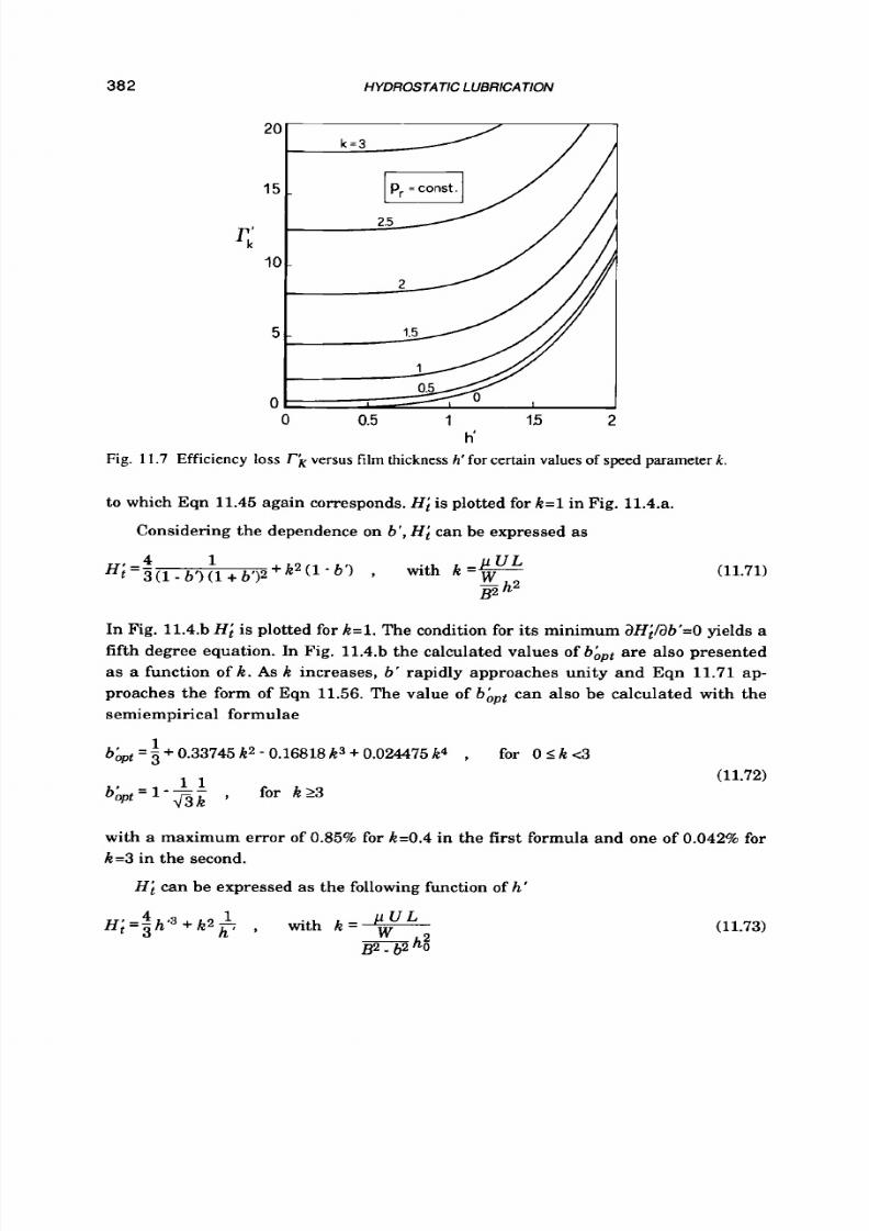
8/9/2019 Hydrostatic Lubrication 1992
http://slidepdf.com/reader/full/hydrostatic-lubrication-1992 399/558
382
HYDROSTATIC LUBRICATION
0
0.5
1 15 2
h'
Fig.
11.7
Efficiency loss r~ ersus film
thickness
h' for certain values of speed parameter
k .
to which Eq n 11.45 aga in corresponds. HI is plotted for k = l in F ig . 11.4.a.
Considering th e dependence on
b',
Hi can be expressed
as
4
1 I I TIT.
In Fig. 11.4.bH i is plotted for k = l . Th e condition for
its
minimum dH;/db'=O yields a
f if th degree equa tion. In Fig. 11.4.b th e calculated values of
bbpt
ar e a lso presented
a s a function of
k .
A s k increases, b' r ap id ly approaches un i ty an d Eqn 11.71 ap-
proaches the form of Eqn 11.56. The value of bhpt can a lso be calcula ted with the
semiempir ical formulae
1
bbpt =j 0.33745k2
-
0.16818k3
+
0.024475k4
,
for
0 5
k c3
(11
72)
with a max imum error of
0.85%
for k=0.4 n t h e first formula a nd one of 0.042% or
k=3 in t he second.
Hi can be expressed as th e following function of h'
(11.73)
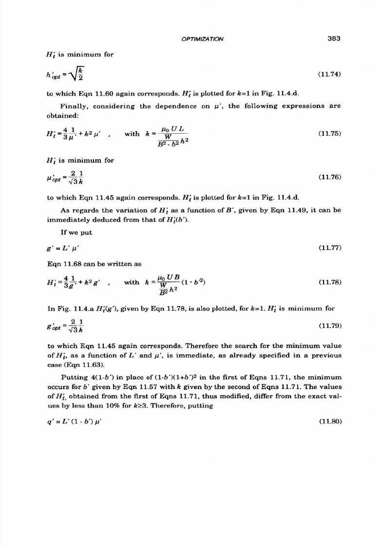
8/9/2019 Hydrostatic Lubrication 1992
http://slidepdf.com/reader/full/hydrostatic-lubrication-1992 400/558
OPTlMlzATlON
383
H i is minimum for
hbpt
=
4
(11.74)
to which Eqn 11.60 again corresponds.
H i
is plotted for K = l in Fig. 11.4.d.
Finally, considering the dependence on p', the following expressions are
obtained:
H i
is minimum for
2 1
P&t
=az
(11.75)
(11.76)
t o
which Eqn 11.45 again corresponds.H i is plotted for k = l in Fig. 11.4.d.
As regards the variation of
H i
as a function of B', given by Eqn 11.49, it can be
immediately deduced from that of
H l ( 6 ' ) .
If we put
g ' = L ' p '
Eqn 11.68
can
be written as
(11.77)
(11.78)
In Fig. 11.4.aH;(g ' ) ,given by Eqn 11.78,is also plotted, for k=1.
Hi
is minimum for
(11.79)
to which Eqn 11.45 again corresponds. Therefore the search for the minimum value
of H i , as a function of L ' and p', is immediate, as already specified in a previous
case (Eqn 11.63).
Putting
4(1-6')
in place of
(l-b')(l+b')z
n the first of Eqns
11.71,
the minimum
occurs for
6'
given by Eqn
11.57
with K given by the second of Eqns
11.71.
The values
of H i , obtained from the first of Eqns 11.71, thus modified, differ from the exact val-
ues by less than
10%
for
k23.
Therefore, putting
q' =
L'
(1 -
6') p'
(11.80)

8/9/2019 Hydrostatic Lubrication 1992
http://slidepdf.com/reader/full/hydrostatic-lubrication-1992 401/558
384
HYDROSTATIC LUBRICATION
in Eqn 11.68, modified and expressed in dimensionless form,
is obtained.
H i
is minimum for
1 1
qApt =
(11.81)
(11.82)
to which Eqn 11.45 corresponds. So for k23 the approximate minimum of H i of Eqn
11.68, considered as a function of L', b', and
p'
is given by Eqn 11.82; it then allows a
wide choice for the three optimum values of L' , b', and p'. The search for the mini-
mum of
H t
given by Eqn
11.68
as a function of
h
and
L,
o r
b, o r
p
can be carried out
in an approximate way, as already seen in the case of constant pressure.
Efficiencv losses. Since W is now assigned, the variation of
H t
is the same as r,
and r, except for T'(h), for which dividing Eqn 11.73by the first of Eqns 11.28yields
r;, 4
h'4
+ k2
(11.83)
Figure 11.8, which is very similar to Fig. 11.7, shows
as a function of h', for k=O,
0.5,1, 1.5,2,2.5,3.
ri
increases very slowly in the range of commonly used values
of
h'.
0 0.5
1
1.5
h'
L
Fig.
11.8
Efficiency
loss rK ersus film
thickness h'
for certain
values of speed parameterk.

8/9/2019 Hydrostatic Lubrication 1992
http://slidepdf.com/reader/full/hydrostatic-lubrication-1992 402/558
OPTlMlzATlON 385
11.6 OPTIMIZATION
The minima of
total
power H , , previously specified, have been determined con-
sidering H t as a function of only one of the variables
L , b , h
and
p
and having taken
B
as
a
reference quantity. The cases in which
it
was considered
as
a function of two
or more variables was actually reduced to the case of only one variable.
We shall now go on to the determination of the minima of Ht as really a function
of two variables which is a rather frequent case in practice since o h n he values of
two variables are assigned, and as a function of three variables which
is
a frequent
case in practice since a t least the value of one variable is assigned, and finally as a
function of all four variables. Optimization is also carried out in the presence of con-
straints of both the variables and of other quantities such as, for example, stiffness
K.
his
is done for the three cases previously mentioned in section
11.2:
given flow
rate, given pressure and given load. Its
application
t o
this last case, that
is
when
the load is assigned,
is
particularly important since this is the condition most fre-
quently encountered in design.
An outline
of
optimization methods, tha t is for the determination of the uncon-
strained or constrained minima of a function, is presented for example in ref.
11.1.
Here sufice it to say that optimization has been carried out with the techniques of
non-linear optimization of the "objective function"
H t ,
for which the Adaptative
Random Search Method proved to be especially suitable. Constraints involved
"penalty functions", for which the Schuldt's Functions proved
t o
be particularly
suitable.
11.6.1
Given
f low
rate
As shown in Fig.
11.2,
Ht only has a minimum as a function of L' , whereas with
the other variables
it
merely increases or decreases.
11.6.1.1
Ht=f(L,b).Equation
11.41
can be expressed in dimensionless form as
(11.84)
where k is given by Eqn 11.43.
In Fig.
11.9
H;(L' ,b ') s plotted in the range O G ' G and
O<b'<l,
for
K = O . l , 1,
10.
In every case
H i
obviously approaches zero as 6' approaches unity
( W
and
K'
also
approach zero while the efficiency losses
r'w(b')
and
rK
(b ' )
decrease).

8/9/2019 Hydrostatic Lubrication 1992
http://slidepdf.com/reader/full/hydrostatic-lubrication-1992 403/558
HYDROSTATIC LUBRlCA TlON
5 8 8
H
1 .88
8.67
8.33
8.88
1.
H
188.88
.88
66.67
.67
3 3 . 3 3
.33
8.88 588 8.7,
a
5 88
Fig. 11.9 Total power H,' versus pad length L' and versus recess
width b;
or viscosity p ' , or
c'=(l-b')p',for certain values
of
speed factor k.
Figure 11.10 shows the results of the optimization ofHi, or OIk112 with the fol-
lowing constraints: lsL'12, 0.2<b'10.6. The constraint L'12 is mostly due to practi-
cal reasons (maximum size); the constraint b'10.6 is due
t o
the fact that both
W
and
K
must be included in a range of convenient values (see Fig. 11.2.b).
H i m
is plotted
with the corresponding optimum values of Lip t and bhpt. Figure 11.10
also
shows
HFk,
H i , p ; coinciding with H i W' iven by the second
of
Eqns 11.11, K coinciding
with W' and
(11.85)
It must be pointed out that
bbpt
takes the higher of the two boundary values, that
is 0.6. Therefore, if a supply
flow
rate is assigned and the search concerns the val-
ues of LApt and
bbpt
for which dissipated power is minimum, bhpt
is
assumed
to
be
equal to the maximum value of
b'.
As regards
Lbpt
it is determined from Eqn 11.44
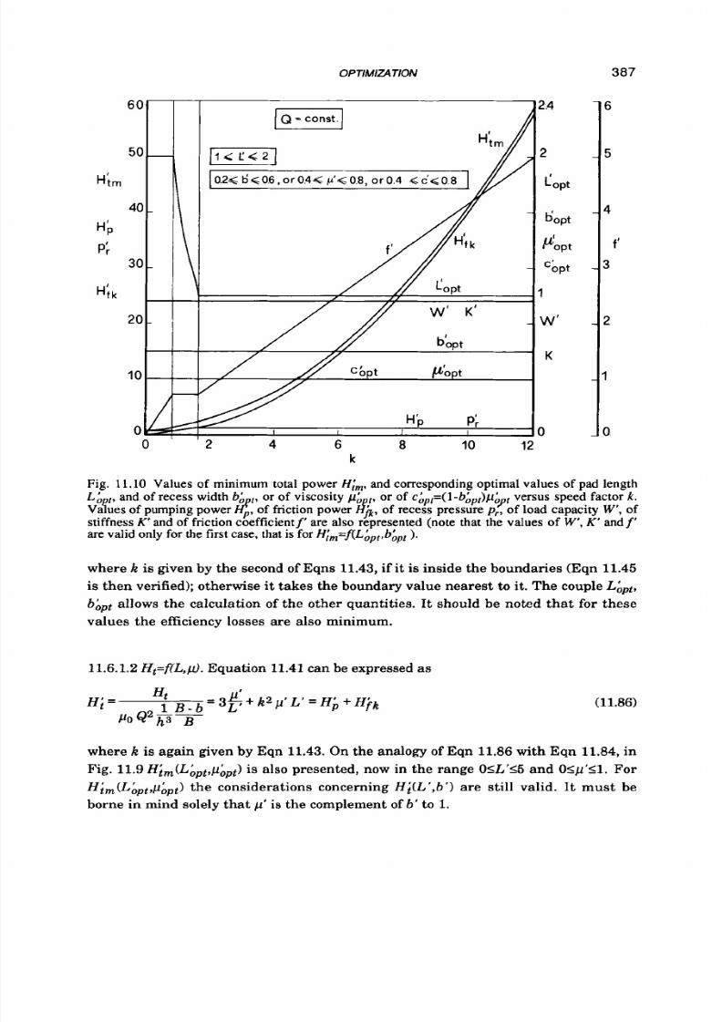
8/9/2019 Hydrostatic Lubrication 1992
http://slidepdf.com/reader/full/hydrostatic-lubrication-1992 404/558
60
5c
Him
Hb
p’,
H;
4c
30
20
10
0
0
Q = cons t .
I
2
4 6 8 10
1
4
?
Copt
bopt
P b p t
C’
opt
a‘
K
387
6
5
4
f‘
3
2
1
3
k
Fig.
1
1.10 Values of minimum total power Hi,,,, and corresponding optimal values of pad length
LApf, nd of recess width
b i ,,
or
of
viscosity pA f
or of c&=(I-b&)p+
versus speed factor
k .
Values of pumping power 4, f friction power fib,
of
recess pressure pr,
of
load capacity
W’,
of
stiffness
K‘
and of friction coefficientf’ are also represented (n ote that the values
of
W’,
K’
ndf’
are valid only for the first case, that is for Hi,, ,=f(L&f,b~pl.
where
k
is given by the second of Eqns
11.43,
f it is inside the boundaries (Eqn
11.45
is then verified); otherwise it takes the boundary value nearest to it. The couple L&,
6APt
allows the calculation
of
the other quantities. It should be noted that for these
values the efficiency losses are also minimum.
11.6.1.2Ht=f(L,p).Equation 11.41 can be expressed as
(11.86)
where k is again given by Eqn
11.43.
On the analogy of Eqn
11.86
with Eqn
11.84,
n
Fig.
11.9Him(L&,t,p&)
is also presented, now in the range
OSL’<5
and
OSp’S1.
or
Hj,(LApt,p&,,pt)
he considerations concerning H i ( L
‘,6‘)
are still valid. It must be
borne in mind solely that p ’ is the complement of 6‘ t o 1.

8/9/2019 Hydrostatic Lubrication 1992
http://slidepdf.com/reader/full/hydrostatic-lubrication-1992 405/558
388 HYDROSTATIC LUBRICATION
Similarly Fig. 11.10 may be used
t o
obtain the results of the optimization of
H;m(L&,,pt,~&,t) ith the constraints lILY2,0.41~'10.8.Figure 11.10 also shows Hjk,
H i andp; ( which coincides with Hi), whereas W and
K'
are given by the second of
Eqns 11.15 andf 'by the following equation
It is obvious th at p ' has always taken the lower of the two boundary values, that
is
p&0.4.
To obtain
Him(L&,p&),
a procedure similar t o tha t for
H;m(L;Zpt,b&,,pl)
is
followed.
11.6.1.3 H,=frL,p,b). Equation 11.41can be again expressed a8
Hi=--
1 - 6 '
1
Ht
- 3 p ' r @p'
(1 6 ' ) L '
POQ2 jp
(11.87)
where k is again given by Eqn 11.43. After having introduced Eqn 11.50, we can also
express Eqn 11.87 as
(11.88)
'
Hi = 3
L';
+
k2 c'
L'
On the analogy of Eqn 11.88 with Eqn 11.86, H~m(L&,,pt,c~p,pt)s also presented in
Fig. 11.9, now in the O G ' S 5 and O<c'<1 range. Similarly, fig. 11.10 may again be
used to obtain cApt and the optimal values of Hirn,
H@,
H i and
p; (
which coincides
with Hi) in the case in which
X L ' a , 0.4<c'10.8.
Friction f is given by Eqn
11.85. W
is determined with the equation
as
well as
K'
which coincides with
W'.
After Eqn 11.50 has been introduced, Eqn
11.89
becomes
(11.90)
W =
3 (1+ 6')
c'
that for c'=constant increases linearly with
6'.
cAPt has always taken the lower of the two boundary values 0.4 and any couple
of
To
obtain Him(L&&,pt), that is
H~m(L~p,p t ,6~p,p , ,&,p ,p t ) ,
procedure similar
t o
that
values of b ' and
p'
satisfying
(1-6')p'=0.4 is
an optimum couple.
for Him(L',6') is followed.
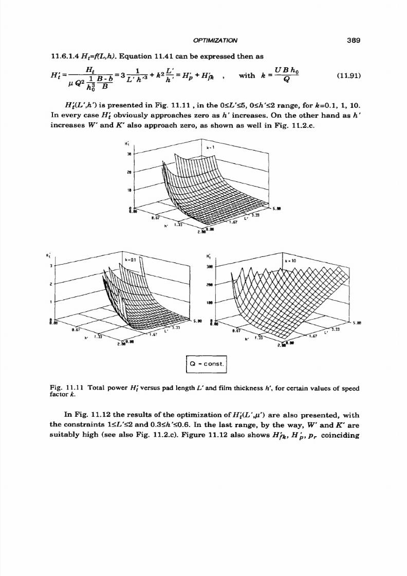
8/9/2019 Hydrostatic Lubrication 1992
http://slidepdf.com/reader/full/hydrostatic-lubrication-1992 406/558
OPTIMIZATION
389
11.6.1.4 Ht=KL,h). Equation 11.41 can be expressed then a s
U B
o
HI=
1 B - b = 3 s + k 2 , = H i + H j k , with k=-
(11.91)
Ht
1 L'
P Q 2 j p B
h Q
H;(L',h') is presented in Fig. 11.11
,
n the OIL'<5,O<h'<2 range,
for
k=0.1, 1, 10.
In every case Hi obviously approaches zero as h ' increases. On the other hand
as
h'
increases
W
and K' a l s o approach zero, as shown as well in Fig. 11.2.c.
Fig.
1 1 . 1
1
Total power
H;
ersus pad length
L'
and
film
thickness
h', for
certain values
of
speed
factor
k.
In Fig. 11.12 the results
of
the optimization o f H & L ' , p ' )are also presented, with
the constraints 15L.12 and 0.3<h'<0.6. In
the last range,
by
the way, W and
K
are
suitably
high (see also Fig. 11.2.12). Figure 11.12 also shows H)h, H i ,
p r
coinciding

8/9/2019 Hydrostatic Lubrication 1992
http://slidepdf.com/reader/full/hydrostatic-lubrication-1992 407/558
390
250
200
H k l
150
HP
p;
100
H;k
50
0
0
' 2
HYDROSTATIC LUBRICATION
4
6
8
I 0
12
k
2.5
0
W'
.5
K'
10
.5
1
Fig.
11.12
Values
of
minimum total power
Hi,,,, and
corresponding optimal values of pad length
L &
and of
film
thickness
h&.
versus speed factor
k.
Values of pumping power
H i ,
of friction
power H j k , of recess pressure p, , of load capacity
w',
f stiffness 1y'and of friction coefficientf'
are also represented.
with
Hi,, W'
and
K
given by the second and third of Eqns
11.13,
espectively. The
friction coefficient is given
by
(11.92)
It should be noted that hAp,Pthas always taken the higher of the two boundary
values:
0.6.
Therefore,
to
obtain
Hi,(L&,t,hAp,Pt),
the maximum value of
h'
must be
selected for
h&,
while
LApt is
determined from Eqn 11.44, hat
is
d 5 1
LApt
=--
k h&
(1
1.93)
If this last value is outside the range of possible values for
L',
the nearest boundary
value will be assumed t o be
LApt.

8/9/2019 Hydrostatic Lubrication 1992
http://slidepdf.com/reader/full/hydrostatic-lubrication-1992 408/558
391
11.6.1.5 H,=f(L,b,p,h). Equation 11.41 can be expressed finally as
(11.941
where
k
is again given by the second of Eqns
11.91.
Figure
11.13.a
shows the results
of the optimization of
Hi(L',b',p',h'),
with the constraints
l I L ' i 2
,
0.21b'I0.6 , 0 .31h ' l0 .6
,
0.81p'11.6 (11.95)
Fig.
11.13
a lso shows
H@,H i p;
coinciding with
HbJ
and
w
,
K'T
' = p
h 3
, 1 - b''
(11.96)
(11.97)
It should be noted that
bbpt
as well as
hApt
and PApt always taken boundary val-
ues: the higher for b' and h' , the lower for p ' , that is bApt=0.6,hApt=0.6 and pApt=0.8.
Therefore, t o obtain
H ; , ( L ~ p t , b ~ p t , p ~ p t , h ~ p t ) ,
he maximum value of b' and h' must
be selected for
bbpt
and
hApt,
while the minimum value of
p'
must be selected for
PApt.
LApt
is
determined from Eqn
11.93,
if
it
is inside the boundaries; otherwise it
takes the boundary value nearest to it.
With Eqn 11.50, Eqn 11.94 can also be expressed as
C ' L'
c'
Hi= 3- , h,3 + k 2 F
(11.98)
In Fig.
11.13.a,
therefore,
Hi,,,
also represents
Hi,(LApt,hApt,c~pt),
obtained with the
constraints
l S L ' I 2
,
0.32Ic'11.28
,
0.3Ih'10.6 (11.99)
cApt has always taken the lower of the two boundary values, i.e. 0.32. Any couple of
values of b' and
p'
satisfying
(1 b' )p'
=
0.32
(1 .100)
is an optimum couple.
To obtain
Hi,(L~p,pt,h~pt,cApt)
he procedure is the same as in the previous cases
but now, since we always have
cbpt=chin
and (from Eqn
11.50) c~i n=( l -b ~, , , )p hin ,
we obtain
bApt=b&
and pLpt=phin.
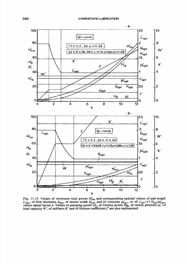
8/9/2019 Hydrostatic Lubrication 1992
http://slidepdf.com/reader/full/hydrostatic-lubrication-1992 409/558
392
HYDROSTATIC LUBRICATION
- a
-
100
80
H;
m
Hb
p;
60
40
H;k
20
0
k
- b -
2.5
Copt
Gopt
hbpt
Pbpt
cbpt
2
1.5
1
0.5
f '
0
100
2.5
Copt
bopt
H i m
hbpt
PLbpt
HP
p;
H;k
opt
80 2
60 1.5
40
1
C'
2 0 0.5
f '
0 0
k
Fig.
11.13
Values of minimum total power Hirn, nd corresponding optimal values of
Lhpl, of film thickness
h C I ,
of recess width
bhpr,
nd of viscosity &
,,
or of cipl=(l
versus speed factor k . Values of pumping power H i , of friction power
&h,
f recess pre
load capacity
W ,
f stiffness
K
and
of
friction coefficientf
are
also represented.
10
8
w'
6
K'
4
2
0
10
8
W'
6
K'
4
2
0
I
ength
'ep, ,
of
pt)Phpr*

8/9/2019 Hydrostatic Lubrication 1992
http://slidepdf.com/reader/full/hydrostatic-lubrication-1992 410/558
OPTlMlZ4TlON
393
In Fig. 11.13.b the results are presented with the same constraints for L' and
p',
but with
0.2
5
b'
1
.9
,
0.3
5
h'
I0.4 (11.101)
We must point out that in this latter case load capacity is the same as in the former
case, but stiffness is
50%
higher
(this
can be immediately deduced from Eqns 11.961,
even with lower dissipated power and a much lower friction coefficient. The same
figure
also
shows the results obtained with the constraints
l l L ' 1 2 0 . 0 8 l ~ ~ 5 1 . 2 8 0.35h'l0 .4
and now chpt=0.08.
EXAMPLE
11.1
The pad of Fig. 11.1, with width B=0.1
m
and length LQ-B, is directly supplied
by a pump as in Fig. 1 l.l.a . The pump isassumed to supply a constant
f low
Q=5.10-6
m31s, that is a little higher than hydrodynamic flow rates. We want to evaluate the
pad load capacity W and stiffness K in the condition of minimum total dissipated
power Ht, for speed U=0.3, 1 ,3 mls .
H t , can be calculated following the first procedure described
in
section 11.6.1.5.
I f the reference value of the film thickness is assumed to be ho=lO-4
m,
factor k,
given by Eqn 11.91, for the three values of speed, takes the values k=0.6, 2, 6. I f , for
example, Constraints 11.95 are adopted, the following results are obtained (also
directly from
Fig.
11.13.a):
1) k=0.6
Lhpt=2, bApt=0.6, h Apt,pt=0.6,
IJ ApFO.8
W'=3.56, K'=5.93, f'=o.18
LoPt=0.2
m,
bopt=O.06m, hopt=0.6.10-4
m
Ht,=6.52 Nmls, Hp=5.56 Nml s, H ~ 0 . 9 6 mls, p,=11.1.105 Nlm2
W=1.78.104 N, K=8.89.1@ Nlm, f=1.8.104.
H;,=2.61, Hi=p; =2.23, Hb=0.384
from which, in dimensional form,
and, taking
as
reference viscosity &=0.1 Nslm2, hpt=0.08Nslm2 and
It should be noted that the value of pressure is not much higher than the values of
hydrodynamic supply pressure and the very low value of the friction coefficient.
2) k=2
Lopt=O.145 m, bOpt=0.06
m,
hOpt=0.6.1O4m, ~pt=0.08A?slmz
Ht,=15.4 NmIs, Hp=Hf =7.7N m l s , p,.=15.4*1@ Nlm2
W=1.78-104N, K=8.89.1@ Nlm, fd.35.1Q4
It should be noted that assuming, for example, the recess depth to be h,=0.08 m, the
power dissipated in it for friction would be Hfp=8.7.10-aN m l s (section 11.5.2.1), just
8/9/2019 Hydrostatic Lubrication 1992
http://slidepdf.com/reader/full/hydrostatic-lubrication-1992 411/558
394 HYDROSTATIC LUBRICATION
a little higher than 1% of Hf. Assuming the lubricant density to be p=900 IQlrn3, the
power dissipated to accelerate it in the film would be H1=5.63.10-4Nmls, less than
0.01 % of Hf.
3)
k=6
Lopt=O.
m, bOpt=0.06m, hOpt=O.6.104m, bpt=0.08Nslm2
Htm=59.1Nm ls , Hp=ll.l Nml s, Hf=48Nmls, pr=22.2-105Nlm2
W=1.78.104N, K=8.89.1@ Nlm, f=9.104
We must point out that the value of load capacity, identical in the three cases, is
suff icien tly high; that o f stiffness, also identical in the three cases, is high
(comparable to that of the deformation of a roller slide-way substituting the pad).
4) I f constraints 11.95 are also considered, though in the form of Eqns 11.99, on the
basis of the second method explained in section 11.6.1.5, or again from Fig. 11.13.a,
we obtain, for example for the case in which k=2:
and for Hirn, Hb=p; and H b and the corresponding dimensional quantities, the
same values obtained in such a case. According to Eqn 11.100 we can now put, for
example, bhpt=0.8 and consequently pbpt=1.6,obtaining
and
Therefore, comparing this case to the second, for the same values of dissipated
power and supply pressure, there is an increase in load capacity and stiffness of
over 12% and a reduction in friction coefficient of over 16%.
5)
Pad efficiency can be improved further by changing the constraints.
So
i f in
Eqns 11.95 new upper boundaries are introduced for b' and he, or example: b'10.9
and h'10.4, that is, i f the constraints 11.101 are considered, according to the second
above-mentioned method in section 11.6.1.5, or from Fig. 11.13.b, we obtain, for
example, for the case in which k=2:
from which
L&=1.45* bhPt=O.32, h
hpt=0.6
W'=4, K=6.67, f'=0.16
W=2*104 , K=1@ Nlm, f=1.6.10-4.
L
Apt=
1, bbpt=0.9,
h
&=0.4,
pApt=O.8
Lopt=O.l m, bopt=0.09m, hOpt=0.4.1O m, kpt=0.08 Ns lm2
Htm=11.38 W, Hpz9.38 W, Hf=2 W, pr=14.1.105 Nlm2
W=1.78.104 N, K=1.34-1@Nlm, f=1.13.104.
Therefore, comparing this case to the second, for the same load capacity, there
is
a
50%
increase
in
stiffness, a 35% reduction in dissipated power, a 9% reduction in
pressure, while the friction coefficient has become four times smaller.
6) It should be noted that without changing constraints the results can be modified
by changing the reference values of the constrained quantities.
So,
i f the dimen-
sional constraints allow it, we can put B=0.2
m.
Therefore, for U=l mls , for exam-
ple, Eqn 11.91 gives k=4 and consequently:
8/9/2019 Hydrostatic Lubrication 1992
http://slidepdf.com/reader/full/hydrostatic-lubrication-1992 412/558
OPTlMlzATlON 395
LoPt=0.2m, bOpt=O.12m, hOpt=0.6.104m, bpt=0.08Nslrnz
Htm=32.4 NmIs , Hp=ll.l Nmls, Hf=21.3 NmIs, pr=22.2.105 Nlm2
W=7.12.1@ N, K-3.56.109Nlm, f=3.104.
We must point out that, as compared to the second case, the dissipated power is
almost doubled, pressure is increased by
50%
but load capacity and stiffness are
four times higher while the friction coefficient is decreased.
IL on the contrary, because of considerable surface roughness and errors in
parallelism, we want to increase fi lm thickness, we can put, for example, ho=2.lO4
m, so that, again for U=l ml s, Eqn 11.91 again gives k=4 and consequently:
Lopt=O.lm, bopt=O.06m, hOpt=l.2.lO4m, kpt=0.08Nslmz
Htm=4.06 Nm ls, Hp=1.39 Nmls , Hr2.67 Nm ls, pr=2.78.105Nlm2
W=0.22-104N, K=0.185.108 lm, f=12.10-4.
It should be pointed out that, again as compared to the second case, total power and
pressure are reduced to almost a fourth and to less than a fifth, respectively, while
load capacity and stiffness are reduced to an eighth and to a little less than a fiftieth,
respectively. The friction coefficient is greatly increased.
Finally i f the reference viscosity is increased, for example, to the value po=0.2
Nslmz, while we still have U = l
mls, k
is
again that of the second case. Therefore all
the dimensionless quantities remain the same, as well as Lop&
bopt and
hopb
while
popt and consequently Ht,
Hp,
Hf, pr, W and K are double. f is the same as
in
the
second case.
11.6.2 Given pressure
As
shown in Fig. 11.3, Ht has a minimum when it i s considered t o be a function
of each variable except forL.
11.6.2.1 Ht=f(b,
h)
11.6.2.1.1.
Equation
11.54
can be expressed as
(1 .102)
In Fig. 11.14 Hi(b‘,h’) s plotted in the O<b’<land OSh’s2 range, for k=O.l, 1, 10.
In all three cases, actually
for
any value of
k,
Hi is minimum for
b’=l
and for h’ in-
creasing with k , starting from zero in the
first
case (actually for
k=O).
Actually, an
investigation in the neighbourhood of point (1,O)has shown that
H i
is equal to zero a t
that point. Hi always approaches zero as 6’ approaches unity and h’ approaches
zero, provided that it happens according t o a suitable law, for example b’=l-ah’p
where a>l and p>l. But investigation has also shown that (1,O)is a singular point:
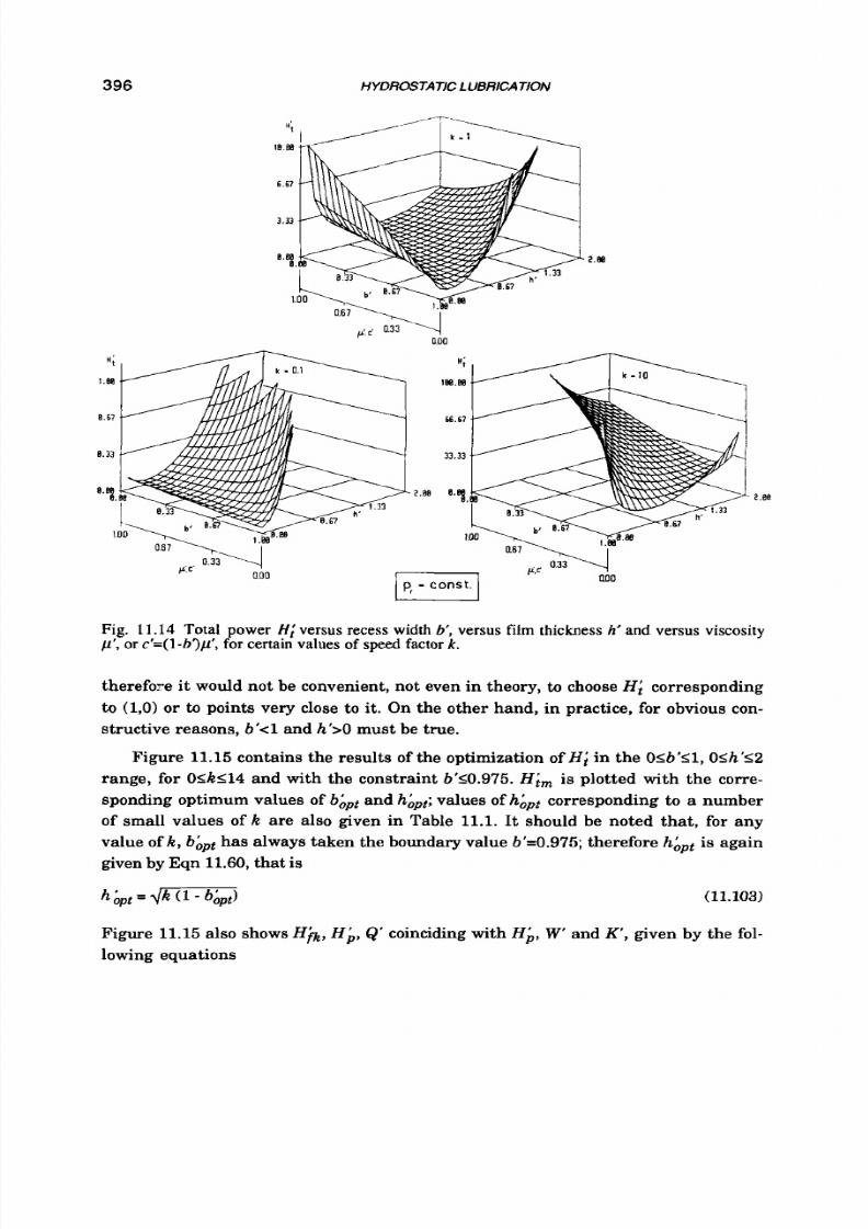
8/9/2019 Hydrostatic Lubrication 1992
http://slidepdf.com/reader/full/hydrostatic-lubrication-1992 413/558
396
HYDROSTATIC LUBRICATION
H;
I8
88
6.67
3 . 3 3
8 .8 8 2.m
1
2.80
Fig.
11.14
Total power
Hi
versus recess width
b',
versus film thickness
h'
and versus viscosity
p' ,
or
c'=( 1
-b l)p ' , for certain values of speed factor k.
therefoye i t would not be convenient, not even in theory, to choose
HI
corresponding
to
(1,O)
r to points very close t o it. On the other hand, in practice, for obvious con-
structive reasons,
b'<l
and
h'>O
must be true.
Figure 11.15contains the results of the optimization of H i in the OSb'Sl,O Sh' S2
range, for OSkg14 and with the constraint b'S0.975. HI, is plotted with the corre-
sponding optimum values of bApt and
hipt;
values of hApt corresponding to a number
of small values of k are also given in Table
11.1.
t should be noted that, for any
value of
k , bApt
has always taken
t h e
boundary value b'=0.975; herefore
hApt
is again
given by Eqn
11.60,
hat is
(11.103)
Figure 11.15also shows
Hb,
L, ' coinciding with HL,
'
and K', given by the fol-
lowing equations
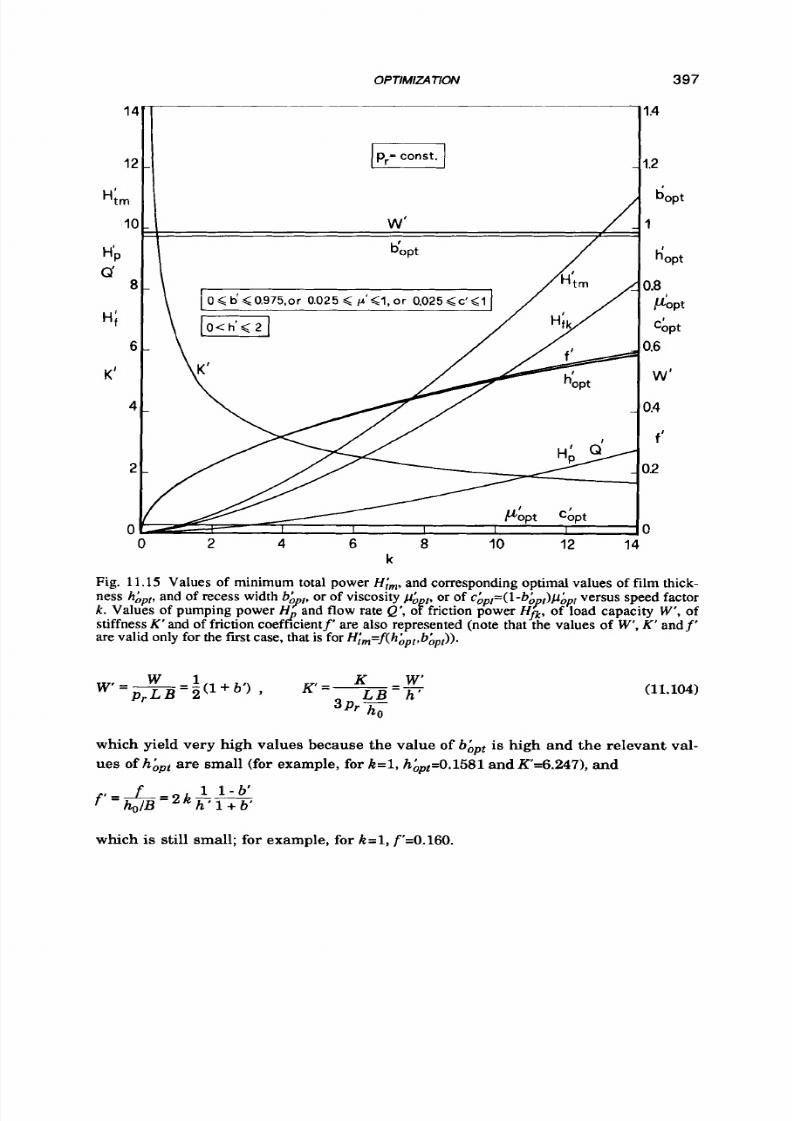
8/9/2019 Hydrostatic Lubrication 1992
http://slidepdf.com/reader/full/hydrostatic-lubrication-1992 414/558
OPTlMlzATlON
397
0< 6
<
0.975.or 0.025
<
~ ' 9 1 ,
r 0.025 <c'<l
0
2 4
6 a 10 12 14
k
Fig.
11.15
Values of minimum total power H;,,,, and corresponding optimal values of film thick-
ness
h&,,
and of recess width
b+,
or
of
viscosity &, ,or of
c&,r=(l-b+r)p&,l
versus speed factor
k. Values of pumping power H and
f l o w
rate Q',
of
friction power Hfi of load capacity
W', of
stiffness K 'and
of
friction coe ffh en tf' are also represented (note that the values of
W',
K' andf'
are
valid
only
for the first case, that is for
H~,,,=f(h&,t,b~p,)) .
(11.104)
which yield very high values because the value of
bApt
is high and the relevant val-
ues of hiptare small (for example, for k = l , h& 0.1581 andK '=6.247), and
f " & = zk - - 1 1 - b '
h ' l + b '
which
is
still sm all; for exam ple, for
k = l ,
f'=O.l60.

8/9/2019 Hydrostatic Lubrication 1992
http://slidepdf.com/reader/full/hydrostatic-lubrication-1992 415/558
398
HYDROSTATIC LUBRlCAT/ON
k
0
hbt
0
0.01 0.025
0.05
0.075 0.1 0.2 0.4
0.6
0.8
0.0158
0.0249 0.0353 0.0433 0.0501 0.0707 0.0999 0.1224 0.1415
Therefore it is to be noted that, for the values of bAptand hApt thus calculated, the
condition of minimum total dissipated power is satisfied as well as that of maxi-
mum load capacity with very high stiffness and a low friction coefficient. Therefore,
if pressure in the recess is assigned, it is convenient to design the pad with the re-
cess as wide a s possible.
Obviously
b’=0.975
is
a limit value. Practical values are lower:
b’=0.95
to 0.75 and
bbpt will take on such values. However the corresponding values of hApt and power
increase while load capacity and stiffness decrease; the friction coefficient also in-
creases. This is proved by the results reported in Fig. 11.16.a, obtained with the con-
straints OSb’S0.9 and O<h’12, and in Fig. 11.17.a, obtained with the constraint
b ‘SO.8.
In conclusion, on the basis of the above considerations, for b’ the maximum pos-
sible value
is
chosen: that is bApt; t is then introduced into Eqn 11.103, thus deter-
mining hApt.
11.6.2.1.2. In practice the condition
OSh’
is replaced by
a s h ’ (11.105)
where a is not too small; this is because of surface roughness and errors in pla-
narity and parallelism, etc., even if the present-day technologies make it possible to
achieve increasingly smaller values of film thickness.
Figure 11.16.b contains the results of the optimization of
Hi(b’,h’),
with the con-
straints
OSb’10.9
and
0.9Sh’SZ
(that is
a=O.9).
For k28.1 the diagrams coincide with
those in Fig. 11.16.a. For 8.bk24.68 only
bApt
and consequently
W’
stil l coincide
while
hbpt=0.9
and consequently H b and
K
become constant;
H ik
decreases more
rapidly while
Him
decreases more slowly than in Fig. 11.16.a. For 4.68>k10.468, we
still have hApt=0 .9 , but W‘ approaches
0.5
and
K’
pproaches 0.5. Moreover
H@=Hb, hat is we again find Eqn 11.45. For 0.468>k20, we still have hAPt=0.9and
bbpt=O.
On the basis of the above considerations, in the presence of constraint 11.105, b’
is again chosen as large as possible and is assumed
to
be bApt; hen from Eqn 11.103
h‘ is determined; if h’ satisfies condition 11.105 i t is h&. If this does not occur, let-
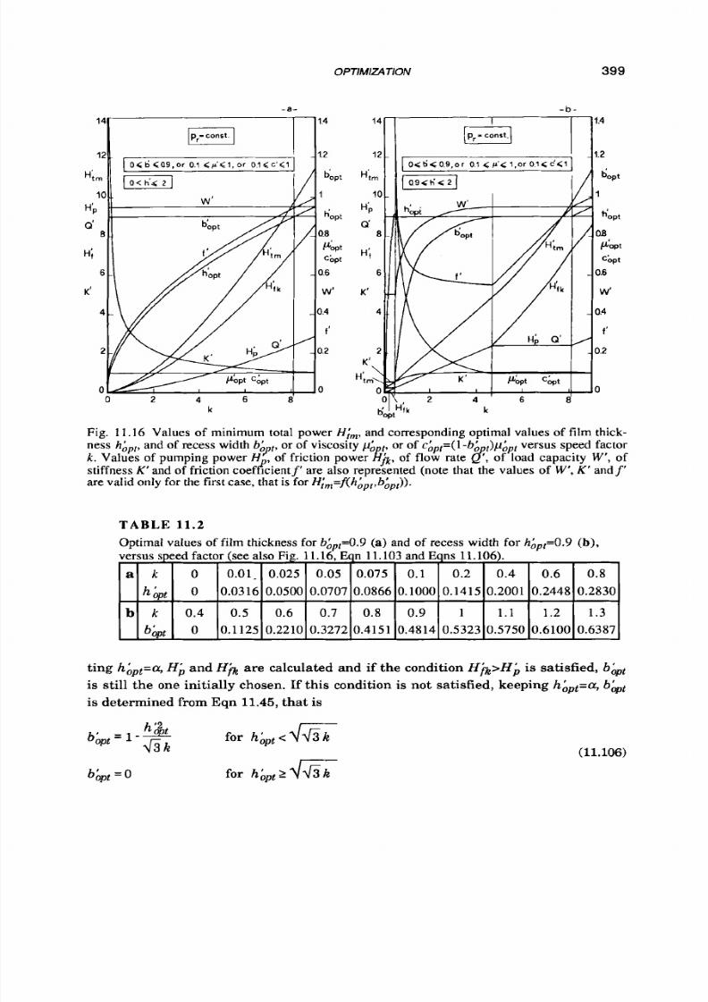
8/9/2019 Hydrostatic Lubrication 1992
http://slidepdf.com/reader/full/hydrostatic-lubrication-1992 416/558
OPTIMIZATlON 399
a k
h&,
b k
bbpt
Fig.
1
1.16 Values of minimum total power H i m , and corresponding optimal values of film thick-
ness
h;,,,,
and of recess width
b
[,
or
of viscosity
&
[,
or of
c&,l=(l-bL
versus speed factor
k.
Values
of pumping power HF of friction power
i j k ,
of flow rate
d ,
f load capacity
W',
of
stiffness K' and
of
friction coeff&entf' are also represented (no te that the values of
W', K'
andf '
are valid only for the first case, that
is
for H;m=f(h&t,b~pr)).
0 0.01. 0.025 0.05 0.075 0.1 0.2 0.4 0.6 0.8
0 0.0316
0.0500
0.0707 0.0866 0.1000 0.1415
0.2001
0.2448 0.2830
0.4 0.5 0.6 0.7
0.8 0.9 1
1.1 1.2 1.3
0 0.1125 0.2210 0.3272 0.4151 0.4814 0.5323 0.5750 0.6100 0.6387
ting hApt=a,H i and H@ are calculated and if the condition
H @ > H i
is satisfied, b&
is still the one initially chosen. If this condition is not satisfied, keeping hAPt=a,
bbt
is
determined from Eqn
11.45,
that
is
(1 .106)
T A B L E 1 1 . 2
Optimal values of film thickness for
&&,=0.9 (a)
and of recess width for h&,=0.9 (b) ,
versus speed factor (see also Fig. 11.16,
Eqn 11.103
and
Eqns 11.106).
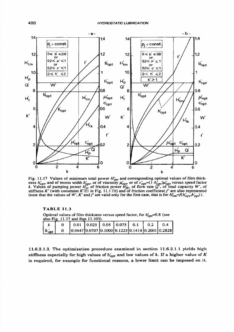
8/9/2019 Hydrostatic Lubrication 1992
http://slidepdf.com/reader/full/hydrostatic-lubrication-1992 417/558
400
k 0 0.01 0.025 0.05 0.075 0.1
It&
0
0.0447 0.0707 0.1000 0.1225 0.1414
HYDROSTATIC LUBRICATION
0.2 0.4
0.2001 0.2828
14/
p,
= const.
1 2 1
p
0
2
k
- a -
1.4
f '
1 0
6
14
12
Him
Hb
H i
10
Q'
8
6
K6
4
2
0
- b -
k
I 4
1.2
bopt
tiopt
PLpt
Gpt
1
1.8
1.6
W'
1.4
f l
1.2
1
Fig.
11.17
Values of minimum total power
H b ,
and corresponding optimal values of film thick-
ness hip, , and of recess width bGI , or of viscosity
&
,,or of c&,,=(l-b~ ,)&,, ersus speed factor
k. Values of pum ping power
H p ,
of friction power of flow rate
Q?
of load capacity
W',
of
stiffness
K'
with constraint
K'21
in Fig.
11.1 7.b) and
of friction coefficientf' are also represented
(note that the values of
W ,
K' ndf' are valid only for the first case, that is for
H;,=f(hApl,bLp,)).
11.6.2.1.3. The optimization procedure examined in section 11.6.2.1.1 yields high
stiffness especially for high values of
bhpt
and low values of k . If a higher value of K
is required, for example for functional reasons, a lower limit can be imposed on
it.
T A B L E 11.3
Optimal values of
film
thickness versus
speed
factor, for b&,,=0.8 (see
also
Fig.
11.17
and
Eqn
11.103).

8/9/2019 Hydrostatic Lubrication 1992
http://slidepdf.com/reader/full/hydrostatic-lubrication-1992 418/558
OPTiMiZ4TloN
40 1
For
Eqn 11.104 where W' is already maximum, since bApt always takes the maxi-
mum value, it all comes down to imposing an upper limit on h'. Indeed, letting
W'
K ' 2
y
,
we have
h ' s -
Y
(11.107)
Figure 11.17.b contains the results of the optimization of Hi obtained with the
constraints OIb'10.8, O<h'12 and K > l . Employing Eqns 11.107, the last two condi-
tions are reduced
to
O<h'sW'/
yand since bhpt=0.8and W'=O.9, they are finally re-
duced to O<h'<0.9.The diagrams differ from those in Fig. 11.17.a in the case of
k>4.05: H i remains constant, Hjk approaches Hi increasing more rapidly, and
hipt=0.9 nd
K'=l.
This is true for any other constraint on b' and
K'.
On the basis of the above considerations, in the presence of the further con-
straints 11.107 on stiffness, b' is still chosen as large as possible and is assumed to
be bhpt; then from Eqn 11.103h ' is determined which is hi p t if it satisfies conditions
11.107;otherwise, hipt=W'/y .
11.6.2.1.4.
From the two previous sections, it follows that if, for practical reasons,
film thickness satisfies condition
11.105
and, for functional reasons, stiffness must
satisfy conditions 11.107, the search for the minimum total power is constrained by
the following conditions:
W'
O s b ' < l ; a s h ' s -
Y
(11.108)
sections.
This search is carried out according to the methods described in the foregoing
11.6-2.2Ht=f(uh)
11.6.2.2.1.
Equation
11.54
can also be expressed as
(11.109)
On the analogy of the first
of
Eqns 11.109 with the first of Eqns 11.102, Hi(p',h') is
also presented in Fig. 11.14, in the Osp'S1 and Osh'12 range. As for Hi(p',h') the
considerations regarding H'(b',h')are still valid.
Similarly in Fig. 11.15 Hirn, hPt and hApt are also plotted, with the constraints
0.0251p'sl
and
0 4 ' 1 2 .
Figure
11.15
also shows
H @ ,
H i
and
Q '
coinciding with
Hi .
W'
and
K'
are easily determined, since W'=1/2 and K=W'lh&,t, while f can be ex-
pressed i n the form

8/9/2019 Hydrostatic Lubrication 1992
http://slidepdf.com/reader/full/hydrostatic-lubrication-1992 419/558
HYDROSTATIC LUBRICATION
PApt has always taken the boundary value p’=0.025; hence, h’ is again given by Eqn
11.60.that is
h&?t
=dmg
(11.110)
Then
Him(p&,t,h&t)
is also presented in Fig.
11.16.a,
with the constraints
O.l<p’<l
and
O<h’12.
Finally
Him(p&,t,hhp,pt)
s presented in Fig.
11.17.a,
with the
constraints
0.25pL1
and
O<h’<2.
In conclusion, on the basis of the above considerations, p’ s chosen
as
small as
possible: it is p&; it is introduced in Eqn 11.110, thus determining h&.
11.6.2.2.2.H;m(p&,h&,t)
is presented in Fig.
11.16.b,
with the constraints
O.lSp’11
and
0.91h’52,
the latter being related to constraint
11.105.
The considerations and conclusions presented in section
11.6.2.1.2
are still
valid; only
bApt
must be replaced by its complement t o one p&, and Eqn 11.103, the
second of Eqns 11.56 and Eqn 11.57 must be replaced by the corresponding Eqn
11.110,the secondof Eqns 11.61and Eqn 11.62.
11.6.2.2.3.H;,(pAPt,h&)
is presented in Fig.
11.17.b,
with the constraints
0.2Sp’11,
(kh’12
and
K‘21,
where the latter two are reduced
t o O<h’10.9,
according to con-
straints 11.107.
only ( l -b&) must again be replaced by p&
The considerations and conclusions deduced in section
11.6.2.1.3
are still valid;
11.6.2.2.4.
Finally, if the search for
H~m(p&,trh&,,pt)
s constrained by the conditions
11.108,
the second of which comes from conditions
11.105
and
11.107,
it is carried out
according to the methods described in the two previous sections.
11.6.2.3Ht=f(b,p,h)
11.6.2.3.1.
Equation
11.54
can also be expressed as
With
Eqn
11.50
Eqn
11.111
becomes

8/9/2019 Hydrostatic Lubrication 1992
http://slidepdf.com/reader/full/hydrostatic-lubrication-1992 420/558
OPTIMlZ4TION
403
(11.112)
On the analogy ofEqn 11.112with the first of Eqns 11.109, H&‘,h’) is also presented
in Fig.
11.14,
in the
O<c’<l
and
O<h’<2
range.
Similarly,
H;,(chPt,pApt)
is also presented in Fig. 11.15, with the following
constraints:
0.025<c’<l , 0 c h ’ < 2 ( 11.113)
H j k , Hi, ’
coinciding with H i are also plotted. Fig.
11.15
also shows
W’, K
(given
by Eqns 11.104)and f ‘ which is
-
f
-
L X -
C ’
f ‘ - ho/B
’
’1
+
b‘ -
‘
’ (1
+
6 ’ )
in the case of b’=0.975=bApt,hat is phpt=l.It must be pointed out that chp,pt=0.025 nd
any couple of values of b ’ and
p‘
satisfying
(l-b’)p’=0.025
s always an optimum
couple. Since chpt has always taken on a boundary value,
hAPt
is given by
h hpt
=
4 d k
phPt
(1 -
bbpt)
(11.114)
H;,(cApt,hApt) is presented In Fig. 11.16.a, with the following constraints:
O . l < c ’ < l
,
O<h‘<2 (11.115)
W’,
K ‘
and f ‘ are also presented as well as the other quantities, in the case of
b’=0.9=bhpt,hat is phpt=l.
Finally, Hi,(chpt,hhp,t) is presented in Fig. 11.17.a,with the constraints 0.21c‘<l
and O<h‘<2. W’, K’ and f ’ are also presented, as well as the other quantities,
b’=0.8=bApthaving been assumed, that is phpt=l.
In conclusion, t o obtain Ht,(bbpt,p~pt,h~pt),’ is chosen as small a s possible:
it
is
chpt; any couple of values of b’ and p’ atisfying
( l -b ’ )p ’= chp t
an be chosen: it is the
optimum couple bbpt, pbpt; such choices can be made on the basis of specific design
requirements.
bhpt
and pbpt are introduced in Eqn 11.114,thus obtaining h&.
11.6.2.3.2. Figure 11.16.b shows H;,(chpt,hbpt) , that
is H
;m(b~pt,p~pt,h~pt)or
(l-b~pt)p~p,p,=chpt,ith the constraints O.l<c’<l and O.9shf<2,the latter of which is
related to condition 11.105. Considerations similar to those presented above, in par-
ticular i n section 11.6.2.1.2, lead us t o the following conclusions:
To find the minimum of H t , in the presence of condition 11.105, c‘ is chosen as
small a s possible. Letting c’=cbptrt is introduced in Eqn 11.114, thus determining

8/9/2019 Hydrostatic Lubrication 1992
http://slidepdf.com/reader/full/hydrostatic-lubrication-1992 421/558
404
HYDROSTATIC LUBRICATION
h‘.
If h’ satisfies condition 11.105 it is h&; otherwise, letting h&=a, H i and H)k are
calculated. If H )p H I; , cApt is still equal to the value initially chosen; otherwise, still
letting h&=a, c& is determined from Eqn 11.45, that is
(11.116)
Any couple of values of
b‘
and p ’ satisfying
(l-b’)p’=c&,t
and
hAPt
form the optimum
combination yielding
Hi,.
11.6.2.3.3. H&&t,h&,t) is
presented in Fig.
11.17.b,
with the constraints
0.21c‘<l ,
O<h’<2 and K’21, the last two of which are reduced to O<h’50.9 from conditions
11.107.
Considerations similar
t o
those presented above, in particular in section
11.6.2.1.3, lead us to the following conclusions:
To find the minimum of
H i ,
in the presence of conditions
11.107, c’ is
chosen as
small as possible. Letting
c’=c&,
it is introduced in Eqn
11.114
obtaining h’. If
h’
satisfies conditions
11.107
it is
hAPt;
otherwise
h&=W’ly .
For the set of optimum
values see section
11.6.2.3.2.
11.6.2.3.4. The search for H t , constrained by conditions 11.108, the second o f which
comes from conditions
11.105
and
11.107,
is carried out according to the methods
described in section
11.6.2.3.2
and section
11.6.2.3.3.
11.6.2.4 Ht= f(L,b,p,h). As seen in section 11.5.3.2, from Eqns 11.55 and Eqns 11.18 we
can deduce tha t the efficiency losses are independent from
L ;
nevertheless the val-
ues of
L
cannot be too large o r
too
small, for many practical reasons. As for real
pads, as mentioned in section
3.3.1, L
is chosen
so
that
B < L I 2 B .
cated in section
11.6.2.3.
In conclusion, having chosen
L , H,,
is obtained according t o the methods indi-
EXAMPLE 11.2
The pad in Fig. 11.1 , wi th m axim um dimensions B=O.l m and L=0.15 m, is
directly supplied by a p um p, as in Fig. 1l . l .a . The supply and recess pressure is
assumed to be p,=106 N lm 2 , that is a l i tt le higher th an in hydrodynam ic lubrication.
We want
to
evaluate load capacity W and stiffness
K
i n t h e c o nd i ti on o f m in im u m
total dissipated power Ht , for speed U=0.3, 1 ,3 m l s .
H t , can be calculated following the procedure described
in
section 11.6.2.3.1.
Then i f ho=10-4m, and
po=O.l
Ns lm 2, the parame te r k, given by the second of Eq ns
11.111, for the three values of speed, takes on the values k=0.3, 1,
3.
I f for example

8/9/2019 Hydrostatic Lubrication 1992
http://slidepdf.com/reader/full/hydrostatic-lubrication-1992 422/558
OPTlMlZ4
TlON 405
constraints 11.115 are adopted, the following results are obtained (also directly from
Fig. 11.16.a):
1) k=0.3
h
bp,pt=O.
173, c;pt=O.l and choosing bApt=0.9, pApt=l
Him=0.0693, Hi=Q'=O.O173, Hb30.052
W=0.95,
K'=5.48, f
'=O.
82
bopt=0.09m, hOpt=0.173~1O4, k p t = O . l
Nslm2
Htm=1.04Nmls,
Hp=0.26Nmls, Hf=0.779Nmls, Q=0.260.106m31s
W=1.43.1@N, K=2.47.108 Nlm, f=1.82.10.4
bopt=0.09m,
h0pt=0.316-10-4 , k p t = O . 1 Nslm2
Ht,=6,32 Nmls,
Hp=1.58Nmls, Hf=4.74Nmls, Q=1.58.106m3ls
W=1.43-1@N, K=1.35.108 Nlm, f=3.33.104
bop,=0.09 m, hOpt=0.548.1O4 , kpt=O.lNslm2
Ht,=32.9 Nm s , Hp=8.22 Nmls, Hf324.6 Nm
s,
Q=8.22.106 m31s
W=1.43.1@N,
K=0.78-108Nlm, f=5.77.10-4.
from which
2) k=I
3)
k-3
It must be pointed out that the value of load capacity, identical in the three
cases, is acceptable as well as that of stiffness, even
i f
this decreases from the first
case to the third one. It should also be noted that,
even
in
the third case, flow rate,
though higher than in the second case and thirty times higher than
in
the first
case, is still not much higher than in the hydrodynamic range.
4) Since, for k=0.3, hoptis too small, again letting ho=10-4 m and, for example,
h'20.4, the method presented in section 11.6.2.3.2 can be followed. Furthermore,
considering cipt=O.lr from Eqn 11.112 we obtain H~=O,O255<0,213=Hi. bpt=0.4 is
then introduced into Eqn 11.116 obtaining chpt=0.308.Also letting bbpt=0.9, we obtain
p'=3.08 and
bopt=0.09m, h0pt=0.4.10-4m, kpt=0.308Nslm2
Htm=2.08Nmls, Hp=Hf=l.04Nm ls , &=1.04.106 m3/s
W=1.43.1@ N, K=1.07.108 Nlm, f=2.43.10-4.
However it should be noted that the total power is almost doubled, stiffness is
reduced to less than a ha lf , while viscosity is too high. A s far as viscosity is con-
cerned, we can make up for it by letting bApt=0.7; hen p'=1.03 and we obtain
bOpt=0.07m, hOpt=0.4.1O4 ,
kpt=0.103
Nslm2
Htm=2.08Nmls, Hp=Hf=1.04 mls, &=1.04.1@6m31s
W=1.275.1@N, K=0.956.108 Nlm, f=2.72.10-4.
As already stated in point 6 in example 11.1, the results can be modified without
changing the constraints but by modifying the reference values of the constrained
quantities.
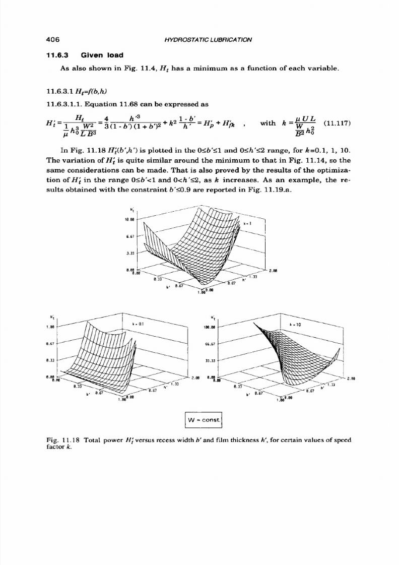
8/9/2019 Hydrostatic Lubrication 1992
http://slidepdf.com/reader/full/hydrostatic-lubrication-1992 423/558
406
HYDROSTATIC LUBRICATION
11.6.3 Given
load
As
also shown in Fig. 11.4,
H t
has a minimum as a function of each variable.
11.6.3.1
Ht=f(b,h)
11.6.3.1.1.Equation 11.68 can be expressed as
In Fig. 11.18
H;(b',h')
s plotted in the OSb'S1 and OIh'12 range, for k=0.1, 1, 10.
The variation of
Hi
is quite similar around the minimum to tha t in Fig.
11.14,
so the
same considerations
can
be made. That is also proved by the results of the optimiza-
tion of H ; in the range O<b'<l and Oeh'12, as k increases. A s an example, the re-
sults obtained with the constraint 6'20.9 are reported in Fig. 11.19.a.
H i
H t
1 . 0 0 100.60
0.67
66.67
8.33
3 3 .3 3
8.88
2 . w 0.88
w
=
COflSt.
Fig. 11.18
Total power
H;
ersus recess width
b'
and
film
thickness
h', for
certain values
of
speed
factor
k.
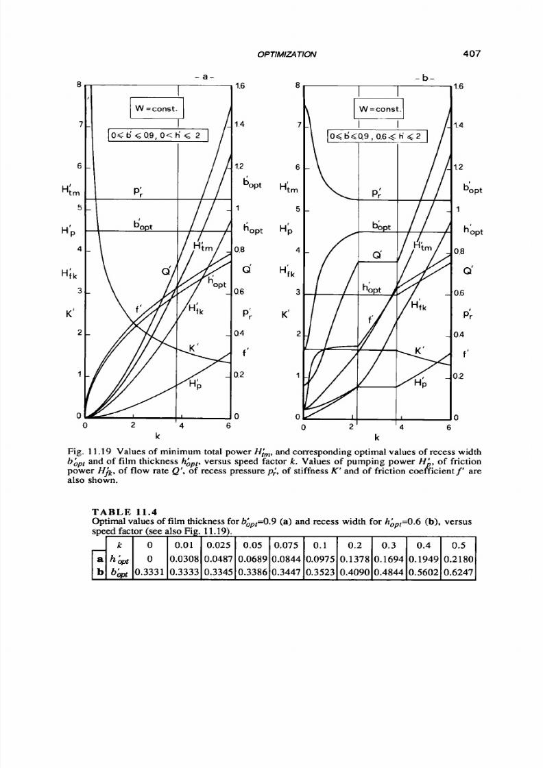
8/9/2019 Hydrostatic Lubrication 1992
http://slidepdf.com/reader/full/hydrostatic-lubrication-1992 424/558
OPTlMlzATION
407
a
b
- a -
1.6
1 4
O < t i ~ O . 9 , 0 < h ’ <
2
k
0 0.01 0.025 0.05 0.075 0.1 0.2 0.3 0.4
0.5
h b t
0.0308 0.0487 0.0689 0.0844 0.0975 0.1378 0.1694 0.1949 0.2180
b&
0.3331 0.3333 0.3345 0.3386 0.3447 0.3523 0.4090 0.4844 0.5602 0.6247
0
0 2 4 6
k
8
1
6
Him
HP
5
4
H;k
3
K’
i
1
0
- b-
0
2 ’ 6
k
Fig. 11.19 Values of minimum total power Him, and corresponding optimal values of recess width
bAp,
and of film thickness
h&,
versus speed factor
k .
Values of pumping power
H’,
of friction
power
Hh,
of flow rate Q’, of recess pressure
p;, of
stiffness K’ nd
of
friction coehicientf’ are
also shown.
T A B L E 11.4
Optimal values of film thickness
for b ,,=0.9
(a) and recess width
for
h&=0.6
(b),
versus
speed
factor
(see also
Fig. 11.19).

8/9/2019 Hydrostatic Lubrication 1992
http://slidepdf.com/reader/full/hydrostatic-lubrication-1992 425/558
408 HYDROSTATIC LUBRICATION
Hirn is plotted with the corresponding optimum values of bbpt and hhpt.Figure
11.19
also shows H @ and H i , as well asp;,
K', Q '
and
f
which are given by the fol-
lowing formulae:
(11.118)
(11.119)
It should be noted that, for any value of
I t ,
bhPt has always taken the boundary
value
b'=0.9;
therefore
hhpt
is found
to
be the one which satisfies Eqn
11.60,
that is
(11.120)
From the above results and with reference to section 11.6.2.1, we deduce that the
optimization with an assigned load must be carried out as follows: b' is chosen as
large as possible: it is bhpt;it is introduced into Eqn
11.120,
thus determining
h&
The couple
bbpt
and
hhpt
makes it possible
to
evaluate the other quantities.
It should be noted that since
bLpt
is as high as possible, consistently with any
other design constraint,
p ;
is the lowest and that since
hbpt
is small, especially for
small
k ,
K is high.
11.6.3.1.2.
If
hhpt
is too small, condition
11.105
can be introduced. Figure
11.19.b
shows the results of the optimization of
H i ,
with the constraints OIb'I0.9, 0.65h'12.
For k23.79 the diagrams are coincident with those in Fig. 11.19.a.For 3.79<kS2.19
bhpt andp; are still coincident but now hhpt=0.6,
o
Q', H i and K become constant;
Hik and H i rn decrease more slowly. For k 2 . 1 9 bbpt decreases, so p; increases, but
we still have
hbpt=0.6, o
K'
remains constant and
Q',
H i
and
Hirn
don't approach
zero as
k
approaches zero. bApt can be evaluated from Fig. 11.4.b o r from Eqns 11.72,
where k is given by the second of Eqns
11.71
into which
hhpt
has been introduced,
that is
(11.121)
In conclusion, as in the case
of
optimization with an assigned load and satisfy-
ing condition 11.105, bhpt is chosen as large as possible, it is introduced into Eqn
11.120, giving h'. Then, if condition 11.105 is satisfied, such a value of h'
is
an opti-
mum value with the chosen
b'.
As a proof, Eqn 11.60 must be satisfied. If condition
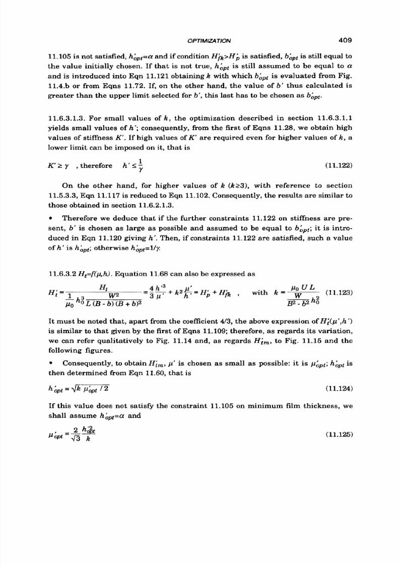
8/9/2019 Hydrostatic Lubrication 1992
http://slidepdf.com/reader/full/hydrostatic-lubrication-1992 426/558
OPTlMlZ.4
TlON 409
11.105 is not satisfied,
hbpt=a
and if condition H h > H ; J s satisfied,
6bpt
is still equal to
the value initially chosen. If that is not true,
hApt
is still assumed to be equal to
a
and is introduced into Eqn 11.121obtaining
k
with which 6kpt is evaluated from Fig.
11.4.b
o r
from Eqns
11.72.
If, on the other hand, the value of 6' thus calculated is
greater than the upper limit selected for
6',
this last has to be chosen as 6&
11.6.3.1.3. For small values of k , the optimization described in section 11.6.3.1.1
yields small values of
h';
consequently, from the first of Eqns 11.28, we obtain high
values of stiffness K . If high values of K' are required even for higher values of
k,
lower limit can be imposed on it, that is
1
K
2
y
,
herefore
h'
-Y
(11.122)
On the other hand, for higher values of k ( k 2 3 ) , with reference to section
11.5.3.3,Eqn 11.117 is reduced to Eqn 11.102.Consequently, the results are similar to
those obtained in section 11.6.2.1.3.
Therefore we deduce that if the further constraints 11.122 on stiffness are pre-
sent, 6' is chosen as large as possible and assumed to be equal to
6hpt;
t is intro-
duced in Eqn
11.120
giving
h',
Then, if constraints
11.122
are satisfied, such
a
value
of h' is h&; otherwise hbpt=lly.
11.6.3.2H,=f(p,h).
Equation
11.68
can also be expressed as
It must be noted tha t, apart from the coefficient4/3, the above expression o f H , ' ( p ' , h ' )
is
similar
to
that given by the first of Eqns
11.109;
therefore, as regards it s variation,
we can refer qualitatively t o Fig. 11.14 and, as regards H i r n , o Fig. 11.15 and the
following figures.
then determined &om Eqn 11.60,that is
Consequently,
to
obtain
Hirn ,p'
is chosen as small as possible: it is
pAPt;hbpt
is
hbpt
=
@-zp
(11.124)
If this value does not satisfy the constraint 11.105 on minimum film thickness, we
shall assume
h&a
and
(11.125)

8/9/2019 Hydrostatic Lubrication 1992
http://slidepdf.com/reader/full/hydrostatic-lubrication-1992 427/558
41
0 HYDROSTATIC LUBRICATION
11.6.3.3 Ht=f(L,h). Equation 11.68 can also be expressed as
long as pApt is replaced by LApt.
The considerations regarding Eqn 11.123 and H i , are also valid in this case, so
11.6.3.4 H,=f(L,jl,h). Equation 11.68 can also be expressed
as
If
we substitute Eqn 11.77 in Eqn 11.127, it becomes
(11.128)
providing p ' is replaced by g'.
The considerations regarding Eqn 11.123 and H i m are also valid in this case,
11.6.3.5 Ht=fi'b,h,/d
11.6.3.5.1. Equation 11.68 can also be expressed as
(11.129)
Figure 11.20.a contains the results of the optimization of H I , in the O<b'<0.9,
O<h'<2,
0.1<p<2 range, for k=O to 6. H i , and the corresponding optimum values
bApt,
hApt
and
phpt
are plotted. Figure 11.20 also shows H @ , H i , p ; and
K'
given by
Eqns 11.118, and
(1 .130)
It must be noted that for any value of
k, bhpt
and
PA pt
have always taken on the
boundary values
0.9
and
0.1,
respectively.
Therefore optimization is carried out as follows:
b'
is chosen as large as possible
while
p '
is chosen as small as possible; they are bhpt and PApt, respectively. The
optimal value of the film thickness is then given by the following equation:

8/9/2019 Hydrostatic Lubrication 1992
http://slidepdf.com/reader/full/hydrostatic-lubrication-1992 428/558
- b -
-
I
t
-
-
-
c
-
41 1
-.a45
0.4
0.35
030
1'
0.2
hT4
0.20
015
:o.lo
0.05
-0
6
"(o.91 40.35
10666
,Q14~<2,or0.l<g<21J
6
k 4
15 45
10 4
35
3.5
H i m
Hb
30 3
5 2:
Q'
<'
p;
20
2
k
15
l.
POP
%
10 1
5
0
3 0
0 ' * k '
Fig. 11.20 Values of minimum total power Hirn, and corresponding optimal values of recess w idth
b&,
of film thickness
h;
, nd of viscosity
&,,. or
of
gAPl=L;,+hp,
versus speed factor k. Values
of
pumping power H;,offriction power ~ h ,f flow rate Q', f recess pressure p;,
of
stiffness K'
and
of
friction coefficient7 are also shown (note that
in
the last case, i.e.
H;,= f (h ; , , , b ~ , , . g L , ) ,
diagrams of
p i
and Q'are valid only when
LAPl=l) .
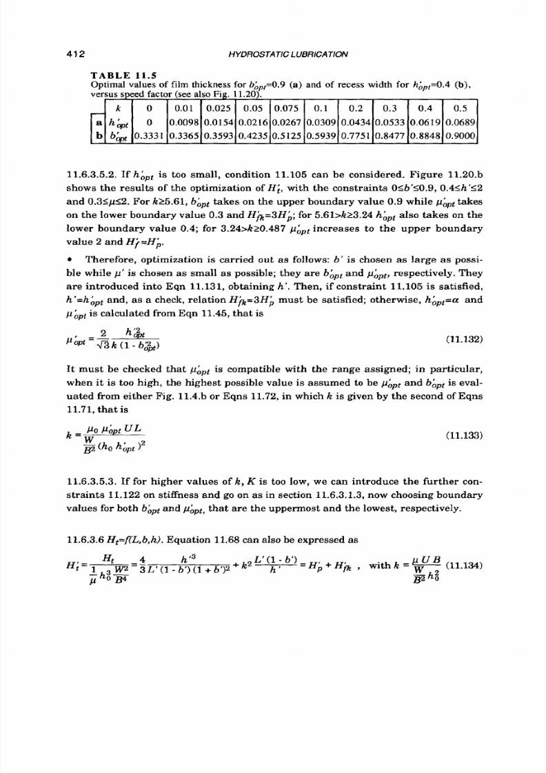
8/9/2019 Hydrostatic Lubrication 1992
http://slidepdf.com/reader/full/hydrostatic-lubrication-1992 429/558
41 2 HYDROSTATIC LUBRICATION
a
b
k 0 0.01 0.025 0.05 0.075
0.1
0.2 0.3 0.4
0 .5
h b t
0.0098 0.0154 0.0216 0.0267 0.0309 0.0434 0.0533 0.0619 0.0689
b& 0.3331 0.3365 0.3593 0.4235 0.5125 0.5939 0.7751 0.8477 0.8848
0.9000
0
11.6.3.5.2. If
hhpt
is too small, condition 11.105 can be considered. Figure 11.20.b
shows the results of the optimization of
H i ,
with the constraints 056'50.9, 0.4Sh'S2
and 0.3Sp52. For k25.61, bApt takes on the upper boundary value 0.9 while PApt takes
on the lower boundary value 0.3 and H@=3Hi; or 5.6bk23.24
hApt
also takes on the
lower boundary value
0.4;
for
3.24>k>0.487 PApt
increases to the upper boundary
value
2
and H+=Hi.
Therefore, optimization is carried out as follows: b' is chosen
as
large as possi-
ble while p ' is chosen as small as possible; they are bApt and PApt, respectively. They
are introduced into Eqn 11.131, obtaining
h' .
Then, if constraint 11.105 is satisfied,
h'=hhptand, as a check, relation H@=3Himust be satisfied; otherwise, h&=a and
phpt
is calculated from Eqn 11.45, that is
(11.132)
It must be checked that
PApt
is compatible with the range assigned; in particular,
when it is too high, the highest possible value is assumed t o be
PApt
and bApt
is
eval-
uated from either Fig. 11.4.bor Eqns 11.72, in which
k
is given by the second of Eqns
11.71,that is
11.6.3.5.3. f for higher values of
k ,
K is too low, we can introduce the further con-
straints 11.122 on stiffness and go on as in section 11.6.3.1.3,now choosing boundary
values for both
bApt
and
pApt,
that are the uppermost and the lowest, respectively.
11.6.3.6
Ht=flz,b,h).
Equation 11.68can also be expressed as
T A B L E
11 .5
Optimal values of film thickness for
b ,=0.9
(a) and of recess width for
hAPl=0.4
(b),
versus speed factor (see also Fig.
11.20).
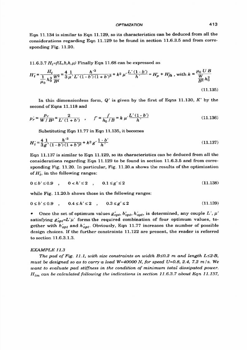
8/9/2019 Hydrostatic Lubrication 1992
http://slidepdf.com/reader/full/hydrostatic-lubrication-1992 430/558
OPTlMlZATlON 413
Eqn
11.134
is similar
to
Eqn
11.129, so
it s characteristics can be deduced from all the
considerations regarding Eqn
11.129
to be found in section
11.6.3.5
and from corre-
sponding Fig.
11.20.
11.6.3.7 H,=f(L,b,h,p)
Finally Eqn
11.68
can be expressed as
(11.135)
In this dimensionless form,
Q'
is given by the first of Eqns
11.130, K'
by the
second of Eqns
11.118
and
Substituting Eqn
11.77
in Eqn
11.135,
it becomes
(1 .136)
(11.137)
Eqn
11.137
is similar
to
Eqn
11.129,
so
its characteristics can be deduced from all the
considerations regarding Eqn
11.129
t o be found in section
11.6.3.5
and from corre-
sponding Fig.
11.20.
In particular, Fig.
11.20.a
shows the results of the optimization
of
H i , in the following ranges:
Ol b ' 10 .9 , O c h ' 5 2 , O. lS g' 12 (1 .138)
while Fig.
11.20.b
shows those in the following ranges:
O< b ' 1 0 . 9 , 0 . 4 1 h ' 5 2
,
0. 31 g' 52 (1 .139)
Once the set of optimum values gApt,bLpt,
h i p t , s
determined, any couple
L' ,
i '
satisfying
gApt=L'p'
forms the required combination of four optimum values, to-
gether with
bhpt
and
h&.
Obviously, Eqn
11.77
increases the number of possible
design choices. If the further constraints
11.122
are present, the reader is referred
t o
section
11.6.3.1.3.
EXAMPLE 11.3
The pad of Fig. 11.1,with size constraints
on
width B10.2
m
and length
L12.B,
must be designed
so
as to carry fa oad
W=40000
,
f or
speed
U=O.S,
2.4,
7.2
m
Is .
We
want to evaluate pad stiffness in the condition of minimum total dissipated power.
Ht,
can be calculated following the indications in section 11.6.3.7 bout Eqn 11.137,
8/9/2019 Hydrostatic Lubrication 1992
http://slidepdf.com/reader/full/hydrostatic-lubrication-1992 431/558
41
4 HYDROSTATIC LUB RICATION
and then with the procedure described in section 11.6.3.5 (but replacing p' with g').
So,
i f
B=0.2 m, ho=2.10-4m and &=0.2 Nslm2, parameter
k ,
given by the second of
Eqns 11.135, takes on the values k=0.8, 2.4, 7.2. Then, with constraints 11.138, for
example, the following results are obtained (also directly from Fig. 11.20.a):
1) k=0.8
So letting for example LLpt=l, p~pt=O.l,
bLPt=O.9, hbp;p,=0.0872, gAp;p,=O.l.
Him=O.0979, Hb=0.0245, Hjk=0.0734, Q'=0.0232, pi=1.05
K = 1.5, f'=0.0918
from which,
in
dimensional form,
LoPt=0.2m, bopt=0.18m, hOpt=O.174.104m, kpt=0.02Nslm2
Htm=3.92 Nmls , Hp=0.979 Nm Is, Hf=2.94 Nm
s,
Q=0.930.106 m3 /s
pr=1.05.1@Nlmz, K=68.8.l@ Nlm, f=0.918.104;
LoPt=0.2
m,
bopt=0.18m, h0pt=0.303~10-4, kpt=0.02 Ns I
mz
Htm=20.4Nmls, Hp=5.09Nmls, Hr 15 .3 Nm ls , Q=4.83.106 m3/s
pr=1.05.1@ Nlm2, K=39.7.1@ N Jm, f=1.59.104;
LoPt=0.2m, bopt=0.18m, hOpt=0.523
lO- 4
m, kpt=O.02 Nsl m2
Htm=105.7 Nmls, Hp=26.4Nmls, Hr79.3 Nmls, Q=25.1.106 m31s
pr=l.05.1
06
N l
m2,
K=22.9-108N l m, f=2.75.104;
2) k=2.4
3) k=7.2
It must be pointed out that in this case and even more so
in
the previous ones,
the value of stiffness is very high.
4) Since in the first case, that is for k=0.8, hoptis too small, the lower limit of h' can
be increased. There would be no benefit in increasing the reference value ho because
we would obtain the same results. Then, with constraints 11.139, for example, the
following results are obtained (also directly from Fig. 11.20. b):
k=0.8
b&O.9, h hp,pt=0.4, g bpt=1.22
so
letting LApt=2
(so
as not to have too high viscosity), pApt=0.608
H im=0.389, Hb=O.194, Ha=O.l94, Q'=0.37, p;=0.527
K=2.5, f'=0.243
from which, in dimensional form,
LoPt=0.4m, bopt=0.18m, hOpt=0.8.104m, kpt=0.122Nslm2
Htm=15.6Nmls, Hp=7.78Nmls, H ~ 7 . 7 8 m/s, Q=14.8.106 m3 /s
pr=0.526.106 N l m2, K=15.1@ N l m, f=2.43.104.
This value of h certainly makes the influence of roughness negligible, and
reduces that of errors on parallelism, while stiffness is still quite high. It should
also be noted that flow rate and supply pressure are not much higher than those
8/9/2019 Hydrostatic Lubrication 1992
http://slidepdf.com/reader/full/hydrostatic-lubrication-1992 432/558
found in hydrodynamic lubrication, while the friction coefficient is at least one
hundred times lower.
11.7 REAL
PADS
11.7.1 Rectangular
pad
We refer to the pad with continuous film and characterized by the relation
(B-b)/2=(L-l)/2=a,
hown in
Fig.6.25,
whose outer corner radius is
r,=O,
as i t gener-
ally is in actual practice. For the sake
of
simplicity and considering that often the
inner radius is also small,
ri=O
is assumed.
11.7.1.1 Given flow rate.
In this case, referring to sections
5.2
and
5.3.5:
3 1 2 B L - ( B + L ) ( B - b )
K = 3 h
W
(L B
+ 2
b)(B
+
b)
'
= 3
/
Q Q (B2-b2)
(1 .140)
(
11.141)
If the pad is in motion, the fluid is subjected to inertia forces; nevertheless,
since the variation of average pressure is negligible (Fig.
6.25),
that
is
also true for
W;
as regards
flow
rate, its decrease on one side is partially compensated by its
increase on the other. The fluid is also subjected to recirculation in the recess but
the phenomenon is negligible at fairly low speed. Therefore, from Eqns
5.106
and
5.108
we obtain
(1 .142)
F =
p
U
Total power is
2'(L
+
b)(B b)
H t = 3 P Q 2 P ~ - ~ + 2 b + C L U
( L
+
b)(B b)
(
11.143)B - b
In dimensionless form,
as
a function of
L'
and
b',
Eqn
11.143
becomes
where k is given by Eqn
11.43. As
a function of
L', Hi
is minimum for
(11.144)
Lbpt
=
1
-
2
b'
+
d ( 1 -2 b')2
-
4 b'(1-b') 1
+
3/12 ( 1 .145)
8/9/2019 Hydrostatic Lubrication 1992
http://slidepdf.com/reader/full/hydrostatic-lubrication-1992 433/558
41 6
HYDROSTATIC LUBRICATION
but obviouslyLhpt21-b’must be satisfied. Lbpt,given by Eqn 11.145
as
a hnction of
b’,
approaches zero as b’ approaches unity.
A s a function of h’,
H i
can also be expressed as in Eqn
11.47
(with obviously a
different reference power) and it approaches zero as h’ approaches infinity. k is
given by the second of Eqns
11.47
multiplied by
(L+ b)(L - B + 2 b)
LZ
(11.146)
As a
function of
p’,
H i can also be expressed as in Eqn
11.48
(with obviously a
different reference power) and it approaches zero as
p’
approaches zero.
k
is given
by the second of Eqns
11.46
multiplied by factor
11.146.
As
a function of all four variables,
HI
can also be expressed a s
(11.147)
where
k
is still given by the second of Eqns
11.91.
9
Its optimization, that is the determination of the values of the independent vari-
ables that make it minimum, can be carried out as in section 11.6.1.5, taking into
account the changes described in this paragraph as regards the above-mentioned
variables. Therefore, the maximum value of
b’
and h’ must be chosen as bhpt and
hhpt,
while the minimum value of p’ must be chosen as
p&. Lhpt
is given by Eqn
11.145
(where
b’=bhpt
and k is given by Eqn
11.43
with h=hhptho)f it is inside its
boundaries, otherwise it takes on the boundary value nearest
t o
it. Other useful
information concerning the optimization of
H ,
can be found in section
11.6.1.
As regards efficiency losses, as a function of L‘ and b‘, Eqns 11.2 yield
L ’ -1 +2 b ’ (L
+
‘b’)(L’-1
+
2 b’)
‘W” 2L’- (L’+ 1)(1+6‘)’ k2 2L’- (L’+ 1)(1+b‘) ’
rK=
rw
As function of L’ they are minimum for
1 1
LhPt= 1.1+ 2-
(11.148)
which is an approximate relation valid only in the 0.51b’Sl and Osk<lO range. A s a
function of
6 ’
their variations are more complex. We can say, as a rough guide, that
they decrease a s b’ approaches unity only for small values of k and high values of
L’.
A s regards the variations of
rb
and
r k
as a function of h’ and
p’,
what has been
stated in section
11.5.3.1
s still valid.

8/9/2019 Hydrostatic Lubrication 1992
http://slidepdf.com/reader/full/hydrostatic-lubrication-1992 434/558
OPTIMIZATION
11.7.1.2 Giuen pressu re. In this case:
41
7
Moreover,
In dimensionless form, as a function of L’ and
b’,
Eqn 11.149 becomes
(1 .149)
(1
.150)
where k is given by Eqn 11.56.HI decreases with L’, while generally it has a mini-
mum when it is considered to be a function of
b’.
As a function of h‘, HI can also be
expressed as in Eqn 11.58 but k must be multiplied by
(11.151)
A s a function of p ’ , H i can also be expressed as in Eqn 11.61, but
k
must be mul-
tiplied by factor 11.151. As a function of h’ and p’ , H i can finally be expressed
as
in
the
first
of Eqns 11.109, where k is given by the second of Eqns 11.109 multiplied by
factor 11.151.
Its optimization can then be carried out as in section 11.6.2.2.1. Therefore,
p’ is
chosen a s high as possible: it is PApt; it is introduced into Eqn 11.110 (together with
the value of k obtained from the second of Eqns 11.109 and multiplied by factor
11.151), thus determining
hAPt.
Useful informations can generally be found in sec-
tion 11.6.2.
As regards efficiency losses Tiy(L’) and r i (L’) , they decrease as L‘ increases,
while
Th(b’ )
nd Ti((b’) generally have a minimum. A s for T i y ( h ’ )and r k ( h ‘ ) ,
what has been stated in section 11.5.3.2 is still valid.
11.7.1.3 Giuen load. In this case:
W L(B+ b)
2 h 3
W (L-B+2b)(B+b)
Q = 3 F m BL
-
(L + B)(B - 6)
r =
2BL
-
(L + B)(B b) ’
Moreover
In dimensionless form, as a function of L’ and b’, Eqn 11.152 becomes
8/9/2019 Hydrostatic Lubrication 1992
http://slidepdf.com/reader/full/hydrostatic-lubrication-1992 435/558
41
8 HYDROSTATIC LUBRICATION
(11.153)
where k=(pUB3)/(h2W).HI(L') always has a minimum, but for much higher values
than those given by Eqn 11.70: for instance, for b'=0.9, the optimal value of
L'
goes
from 6.8 to 1.05 when k goes from
1 o
10.H ; ( b ' ) always has a minimum as well.
Such a value can be approximately evaluated, for L '=l and k>l, from Eqns 11.72 and
increases with L'. As a function of h',
H i
can also be expressed as in the first of
Eqns 11.73 but k now is
(1 .154)
A s a function of p ' ,
HI
can also be expressed as in the first of Eqns 11.75, but
k
must be multiplied by the expression between square brackets in Eqn 11.154.
As
a function of L', b', h' and
p ' , HI
can be expressed as
(11.155)
Po
B4
where
k
is given by the second
of
Eqns 11.135.
Its optimization, for a given value of L ' , can be carried out as in section
11.6.3.5.1, taking into account the changes described in this section. Therefore,
b'
is
chosen as large as possible while p' is chosen as small
as
possible; they are b&,t and
php t , respectively.The optimal value of film thickness follows from Eqn 11.60, that is
(11.156)
When the above value is too small we can
go
on as in section 11.6.3.5.2. Namely, we
assume the minimum possible value to be hApt and obtain phPt from Eqn 11.45, that
is
(1 .157)
If phPtproves
to
be too large it will be necessary to assume the highest possible value
to be pApt and to reduce b';
bhpt
may be approximately evaluated from Eqn 11.72, in
which
k
is given by Eqn 11.133.
As
regards efficiency losses, what has been stated in section 11.5.3.3 is still
valid.

8/9/2019 Hydrostatic Lubrication 1992
http://slidepdf.com/reader/full/hydrostatic-lubrication-1992 436/558
OPTlMZ4TlON 419
EXAMPLE 11.4
Let us consider a pad with width B=O.l m, which must carry a load of 45000 N at
a speed of 0.2 mls. Recess pressure must be lower than 4-106N lm 2 and the friction
coefficient must be lower than 10-4; the lubricant viscosity is
0.03
Nslm2. They are
the same data as in example 5.12 but now
ri=O
is also assumed. Letting ho=0.75.10-4
m and p0=o.03 Nslm2, the speed parameter, given by Eqn 11.135,
is
k=0.0237. For
this value, from Eqn 11.156, we would get
a
ualue of
h
which
is
too small. So let us
impose a lower limit on h and consequently on h': for instance h'10.4. If we select
L'=2 and b'=0.9, Eqn 11.157gives an excessively high value of optimal viscosity; then
we may assume pApt=l and obtain an approximate value of bApt from Eqn 11.72 (after
having calculated k by means of Eqn ll.133), that is bApt=0.36. Then we obtain, in
dimensional form,
and the last three values are coincident with those in example 5.12. Moreover,
bOpt=0.036m, hOpt=0.3O4 m, L=0.2 m, p=0.03 Ns Im2
p,=4.33.1@ Nlm2, &=3.48.106m 3 /s , Hp=15.1Nmls,
Hf=O.6Nm/s, Htm=15.7Nmls, f=0.67.104.
Recess pressure is a little higher than the maximum value given above,
whereas
Q
and Htm are a little lower than the values obtained in example 12.5.
In order to reduce recess pressure one may increase the recess width
or,
more
efficiently, the pad length. For instance, stating L'=2.5, the following values are
obtained: LoPt=0.25m, popt=O.024 s lm2, which
is
a
very
common value and
bOpt=0.037m, p,.=3.21,1@ Nlm2, &=3.44.106 m3/s,
Hp=ll.lNm ls , HrO.7 Nmls, Htm=11.8 Nmls, f=0.80.10-4.
Now pr
is
lower than that in example 5.12.
11.7.2 Other types of pads
The methods presented above are a useful reference for the optimization of other
types of pads, such as, in particular:
cylindrical pads with rectangular recesses (Fig. 5.30)
multipad bearings made of several cylindrical pads, separated by grooves
(Fig. 7.32.a)
multirecess bearings, without grooves (Fig. 8.l .a), in which more complex
phenomena are involved.
The optimization methods described above have shown that often bearings with
wide recesses (high values
of b')
are more convenient. This confirms what is t o be
found in the literature regarding multipad and multirecess bearings. In ref.
11.2
an average value
of
about 0.78
is
proposed while in ref. 8.17 the values suggested by
other authors range from
0.45 t o
0.85.
8/9/2019 Hydrostatic Lubrication 1992
http://slidepdf.com/reader/full/hydrostatic-lubrication-1992 437/558
420
HYDROSTATIC LUBRlCATlON
11.7.3
Circular
pad
The reader is referred t o the bearing in Fig. 5.1.a. If the bearing rotates, the
lubricant is subjected t o inertia forces (section 5.3.61, with a pressure peak at the
inner edge of the recess (Fig. 5.8). This causes a loss of flow rate, slightly hindered
by the inlet (section 5.3.4) and turbulence effects (section 5.3.51,but largely compen-
sated by the increase of load capacity. That justifies the assumption of negligible
inertia forces. The friction torque in the recess is also disregarded.
11.7.3.1 Given f l o w rate. Assuming a linear pressure drop in the film (r2-rl)/r2 in
place of the logarithmic drop ln (r2/r l), the pumping power of the bearing can be
written as
(11.158)
which yields lower values with errors decreasing from 30 t o
3%
as r'=r1/r2 in-
creases from
0.55
to
0.95.
The friction power H f can approximately be written as
H -/ 2 E
f
- h Up
(2 r2)
r2
rl) ,
with Up = 1.7 f2r2
which yields values higher than the exact ones with an error of 30 for r'=0.55 but
lower by 3 for r'=0.95.Thus to ta l power is
which is similar
t o
Eqn 11.41.
A s regards its optimization as a function of one or more of the three variables rl,
h
and
p ,
with
r2
as
the reference quantity, what has been stated about the
H t
of
the
indefinite pad, as a function of
6 , h
and p , with
B
as the reference quantity, can be
applied, approximately, replacing L with (rr12)r2 (given datum) and U with
U p .
n
particular, the remarks made in section
11.6.1.5
are still valid, but now L' can no
longer be considered
t o
be an independent variable, since we still have L'=x12.
11.7.3.2
Given pressure. In this case
8/9/2019 Hydrostatic Lubrication 1992
http://slidepdf.com/reader/full/hydrostatic-lubrication-1992 438/558
OPTIMIZA
TlON 421
which now yields higher values than the exact ones, with the same error as in Eqn
11.158.Total power is then
5c
-
H =--h3
r2 + , U 2 'r2)(r2
-
rl) ,
with Up
= 1.7
R r z
t
3 p p F G h
P 2
(11.159)
which is similar to Eqn 11.54.
The remarks regarding the previous case can be extended to this one.
11.7.3.3Given load. In this case
with the same error as in Eqn 11.158. Moreover the minimum of H p now occurs for
rhpt=113,which is much lower than the exact value 0.529. H f can be written as
H f = f Up2 (2n r2)(rz rl) ,
with U p = 0.85 Rrz
Total power then becomes
(11.160)
which is similar to Eqn 11.68.
The remarks regarding the previous cases can be extended t o
this
one, but now
L must be replaced by
2xr2
(that is we have L ' = ~ K )nd U by
Up=0.85Rr2.
Moreover,
after the evaluation of
bhpt
for the equivalent infinite pad, the corresponding value of
rApt can be calculated from the following equations:
159
rbpt = bhpt
,
for k > 1
rhpt = 100 + 59
k0.04
bhpt
,
for r;
(11.161)
which, approximately, take into account the above-mentioned error corresponding
to the minimum of
H p .
EXAMPLE 11.5
Let us consider a circular pad with diameter D=2rz=0.1
m,
which must carry a
load W=50000 at an angular speed R=25n rad
I s
(same data as in example
5.2).
Letting ho=O.
75.10-4
m, 1.(~=0.009s
Jmz,
L=2mz and U=Up=0.85Qrz,
the
speed pa-
8/9/2019 Hydrostatic Lubrication 1992
http://slidepdf.com/reader/full/hydrostatic-lubrication-1992 439/558
422
HYDROSTATIC LUBRICA TlON
rameter, given by the second of Eqns 11.129, is k=0.0839. For
it,
from Fig. 11.20.a
or
from Table 11.5.a we would get a value of h which is too small.
So,
imposing a lower
limit to
h
and consequently to h’
(for
example h’20,4), from Fig. 11.20.b
or
by inter-
polation from Table 11.5.b we obtain bApt=0.540; hen from the first of Eqns 11.161
from which, in dimensional form, rlopt=0.028 m; hoPt=0.3.104 m, which is much
lower than the value in example 5.2; popt=O.018Nslm2, equal to the value in example
5.2. Then, utilizing of course exact equations, we find
rhpt=0.560, hhp,pt=0.4, C(hpt=2,
pr=10.8.106 Nlm2, Q=14.6.106m31s, Hp=157Nmls,
Hr32.8 Nml s, Ht,=190 Nml s, f=2.1.10-4.
It should be noted that, as r’ decreases to r’=0.529, Htm remains virtually constant.
EXAMPLE 11.6
Let us again consider a circular pad with diameter D=2r2=0.1 m, but which
must carry a load W=lOOOO N at an angular speed l2=300nradls (the same data as in
example 5.4). Letting ho=1.5.104
m,
p,,=0,05 Nslm2, L=2m2 and U=Up=0.85f2r2, he
speed parameter, given by the second of Eqns 11.129, is k=6.99. For it, with the
method described in section 11.6.3.5.1 with the constraints ~(’20.3 nd b’10.9, we
obtain
Thus
the two latter values are both lower than the values in example 5.4. Moreover,
pr=1.41.106 Nlm2, the same value as in example 5.4, Q=141.10-6m31s, Hp=199Nmls,
Hf=671 Nmls , Htm=870 N m l s and f=1.5.103. The power ratio is HfIHp=3.34, not
much higher than the value 3 indicated in section 11.6.3.5.2. This proves that the
optimization method described is sufficiently valid. Obviously, more approximated
values could be obtained by introducing the inertia corrective factors, as in example
5.4. In any case the values of powers and of the friction coefficient are about half
those in that example.
rApt=bhpt=0.9,
h
hpt=0.4#7,
&=0.3.
rlopt=0.045m; hopt=0.67.10-4 , hpt=O.015Nslm2;
11.7.4 Annular pad
The reader is referred to the bearing in Fig.
5.13.
If the bearing rotates, the lu-
bricant
is
subjected to inertia forces, with pressure variations also occurring inside
the recess (Fig. 5.18).They have little effect on average pressure, on flow rate, espe-
cially
for
common values
of
the inner radius (that are never small) (Fig.
5-17],
nd
on load capacity (section
5.4.5).
Therefore the inertia forces can be assumed to be
negligible. The friction torque in the recess can also be disregarded.
8/9/2019 Hydrostatic Lubrication 1992
http://slidepdf.com/reader/full/hydrostatic-lubrication-1992 440/558
11.7.4.1Given
flow
rate.
The relation
(r2-rl)=(r4-r3)=a
is assumed. The closer rl is to
r4,the closer th e former relation is to
r l /
~ 2 = r 3 /4 corresponding t o equal flow rates
through the films. Linear pressure drops in the film ( r 2 - r 1 ) / r 2nd
(r4-r3)/r4
re also
assumed in place of the logarithmic drops 1n(r2/rl)and ln(r4/r3).Finally
1t(r4+r2)
is
replaced, roughly, by ~ r 4 + r l ) .he pumping power of the bearing can then be writ-
ten as
(11.162)
which yields lower values with errors decreasing from 16% to
3%
as r ’ = r l / r 4 n-
creases from
0.5
to 0.9. In Eqn 11.162
~(r4+rl )
nd 2(r4-r3)correspond to L and (B-b)
in Eqn 11.4. The friction power
H f
can also be written approximately as
which yields values lower than the exact ones with an error decreasing from 8%
t o
0.2%
as
r’
increases from 0.5 t o
0.9. As
regards approximations, it should be noted
that as r l goes
to
infinity the bearing turns into an infinite pad. Then total power is
which is quite similar
t o
Eqn 11.41.
As regards its optimization as a function of one or more of the three variables r3
(o r r2 ) ,h and p , with B=(r4-r1) as a reference quantity, what has been stated con-
cerning the total power of the infinite pad as a function of b ,
h
and p , with
B
as a
reference quantity, can be applied here too, replacing L with x(r4+rl) (given datum)
and
U
with
U p .
As far as
r3,
o r
r2
are concerned, they are correlated in an elemen-
tary manner to 6’; we have for example
r,
+
rl
+
(r4
-
rl)b’
2
3
=
11.7.4.2
Given
pressure.
In this case
which now yields higher values than the exact ones, with the same error as in Eqn
11.162.
Total power is then
(11.163)

8/9/2019 Hydrostatic Lubrication 1992
http://slidepdf.com/reader/full/hydrostatic-lubrication-1992 441/558
4 2 4
HYDROSTATIC LUBRICATION
previous case (i.e. section
11.7.4.1)
can be extended
t o this
one.
Equation
11.163
is similar to Eqn
11.54
and the considerations regarding the
11.7.4.3 Given load.
In this case
4 h3 W2
H
=--
P 3
p
n
(r4+ r l) r4 r3) [(r4 rl )
+ r3 - r2)12
with the same error as
in
Eqn
11.162. In
i t
n(r4+rl)/2, (r4-r3), r4-rl)
and
( r3 - r~ )
correspond to L , (B-b),B and b in Eqn 11.25, respectively. The friction power can be
written as
which yields values lower than the exact ones, with an error decreasing from
11%
to
3%
as
rl
increases from
0.5
to
0.9,
which is virtually equal
to
that of H p , especially
for high values
of rl.
Total power then becomes
Equation
11.164
is similar
to
Eqn
11.68
and what has been stated in the previous
cases can be extended to this one, but now L must be replaced by
n(r4+r1)/2
nd U by
Up=1.390(r4+r1)/2.
EXAMPLE 11.7
Let us consider an annular pad with an outer radius r4=0.05 m and an inner
radius rl=0.03m (r'=0.6), which must carry a load W=20000 N at an angular speed
0 = 4 n r a d / s the same data as in example 5.6). Letting ho=0.75.10-4
m,
h=0.05
Ns 1m2, L=n(r4+r3 2, B=r4-rl and U=Up=1.390(r4+rJ 2, the speed parameter, given
by Eqn 11.129,
is
k=O.0156. For it, from Fig. 11.20.a
or
from Table 11.5.a, we would
get a value of h
which is
too
small. So imposing a lower limit to
h
and consequently
to h',
for
example that in Fig. 11.20.b, from the same figure or from Table 11.5.b, we
obtain
bhpt=O.345,hApt=0.4 and pApt=2, from which r3,,=0.0435 m and rZoPt=O.0366m;
hopt=0.3.lO-4
m,
lower than the value in example 5.6;
popt=O.l
Nslm2, equal to the
value
in
that example.
Moreover, p,.=5.92.1O6 Nlm2, Q=10.2.10-6m3/s, Hp=60.3Nmls , H ~ 3 . 0 m ls ,
Ht,=63.3 N m / s and f=3.0.10-4. Furthermore, letting p=900 Kglm 3 and c=1900
JIKgOC, AT=3.6
"c.

8/9/2019 Hydrostatic Lubrication 1992
http://slidepdf.com/reader/full/hydrostatic-lubrication-1992 442/558
OPTlMlZATlON
425
Flow rate, pumping and total power are much lower than those in example
5.6,
but this is due to the lower value of h, obtainable with an accurate construction and
assembling of the bearing.
EXAMPLE 11.8
Let us consider an annular pad with an outer radius r4=0.03 m and an inner
radius r1=0.02 m (r'=2/3), which must carry a load W=2000N at an angular speed
Q=GOOzradjs (the same data as in example 5.10). Letting ho=0.75.10-4 m and
pt,=0.005Nsjm2, the speed parameter, given by Eqn 11,129 with the above-mentioned
substitutions of L and U, s k=0.229 and
for
this, what has been stated in example
5.10 can be applied here
too.
Thus, we obtain
bApt=0.8, hApt=0.4, pipt=2, from which r30pt=0.029m, then a'=O.l, r2,t=0.021 m;
hOpt=0.3.10-4m, lower than the value in example 5.10; popt=O.O1 Nslm2, the same
value as in example
5.10.
Moreover, pr=1.41.106 Nlm2, &=100.106 mais, Hp=141 Nmls, Hf=255 Nmls ,
Ht,=397 N m l s and f=2.71-10-3. Furthermore, letting p=870 Qlm3 and c=1930
JIKgV, AT=2.4
"c.
Flow rate, pumping and total power are definitely lower than those in example
5.10. It should be borne in mind that the above results are based on an approximate
equation ( tha t is Eqn 11.164); indeed it could be proved that for a'=0.1 and
hOpt=0.3.10-4m the optimal viscosity is rather lower, being hp,=0.0074 N s lm2; never-
theless, the total power which tallies with this new value of viscosity is only slightly
lower (Ht,=380 Nmls).
11.8 COMPENSATED SUPPLY
Let us consider the infinitely long pad in Fig. l l . l . c , with width B , supplied by a
pump through a compensating element (Fig. 1 l. l .b) across which pressure drops
from the supply value
ps,
kept constant by a relief valve, to that in the recess
pr
The
performance of a portion of length
L
i s
studied.
11.8.1 Capillary tubes
If the compensating element is
a
capillary tube with diameter
d
and length
L,
equating expression
4.66 to
expression 4.48 yields
(11.165)
where
8/9/2019 Hydrostatic Lubrication 1992
http://slidepdf.com/reader/full/hydrostatic-lubrication-1992 443/558
426
HYDROSTATIC
LUERICATiON
R
= - p -
28
1
r
n d4
is the capillary tube hydraulic resistance and
is the hydraulic resistance
of
the pad. From Eqn
153
we obtain
is the characteristic ratio
of
all compensated bearings. We also obtain
(4.66
rep.)
(6.11rep.)
(6.19 rep.)
11.8.2 Steady pad
11.8.2.1Given pressure. Substitutingpp, forp, in Eqn 4.47 yields
With simple operations (see also section 6.31, we also obtain
(
11.167)
Ps
K = 5 (1 - B )
B
L ( B
+
b )
1 1 L
3 P
=
- -P
pSh3
~ - 6
(11.168)
H =--1 L (11.169)
It should be noted that
Hp =Hpc Hpb
(11.170)
where Hpc=Q(ps-pr) is the power dissipated in the capillary tube, which can be wri t -
ten as
(11.171)
and Hpb=&pr s the power dissipated in the bearing, which can be written as

8/9/2019 Hydrostatic Lubrication 1992
http://slidepdf.com/reader/full/hydrostatic-lubrication-1992 444/558
OPTlMlZ4TlON
427
(11.172)
Comparison of the foregoing equations, for the typical value p = 0 . 5 of the pres-
sure ratio, with the analogous equations in section
11.5.1.2
(direct supply) immedi-
ately shows that, when supply pressure is the same, load capacity is halved, as well
as recess pressure, flow rate and pumping power, and stiffness is reduced to one
fourth. When recess pressure (that is load capacity) is the same, supply pressure
and pumping power are double that found in the case of direct supply, whereas
stiffness is halved.
In
our
investigation into the performance of the pad as p vanes because of the
variation in the dimensions of the capillary tube, diameter
d
an do r length
1 ,
we
assume that the dimensions of the pad are given, as well as film thickness
h
and
viscosity p; he above equations may hence be written in a dimensionless form as
follows
The ratio of Hic and Hib may also be of interest:
(11.173)
(11.174)
(11.175)
which coincides with Eqn
6.19.
The results are plotted in Fig. 11.21.a. From it, the characteristics of a bearing
with assigned dimensions, film thickness (equal
to
the reference value) and supply
pressure can be determined as the capillary tube geometry varies. It must be
pointed out that K
s
maximum for
p=0.5
(as clearly follows from
dKldb=O)
and that
for p=0.3 and 0.7 it still reaches 84%of its maximum value. For this reason it is
commonly recommended to adopt p= 0 .5 o r values close to it. R , / R
is
also plotted in
Fig.
11.21.a.
From that curve, for given bearing dimensions and h , the dimensions
of the capillary tube can be determined.
Eqn 6.19 can also be written in the form
(11.176)
Then, in the investigation into the performance
of
the pad as
p
varies, now assum-
ing the dimensions of the pad and capillary tube are constant (or, better, the ratio
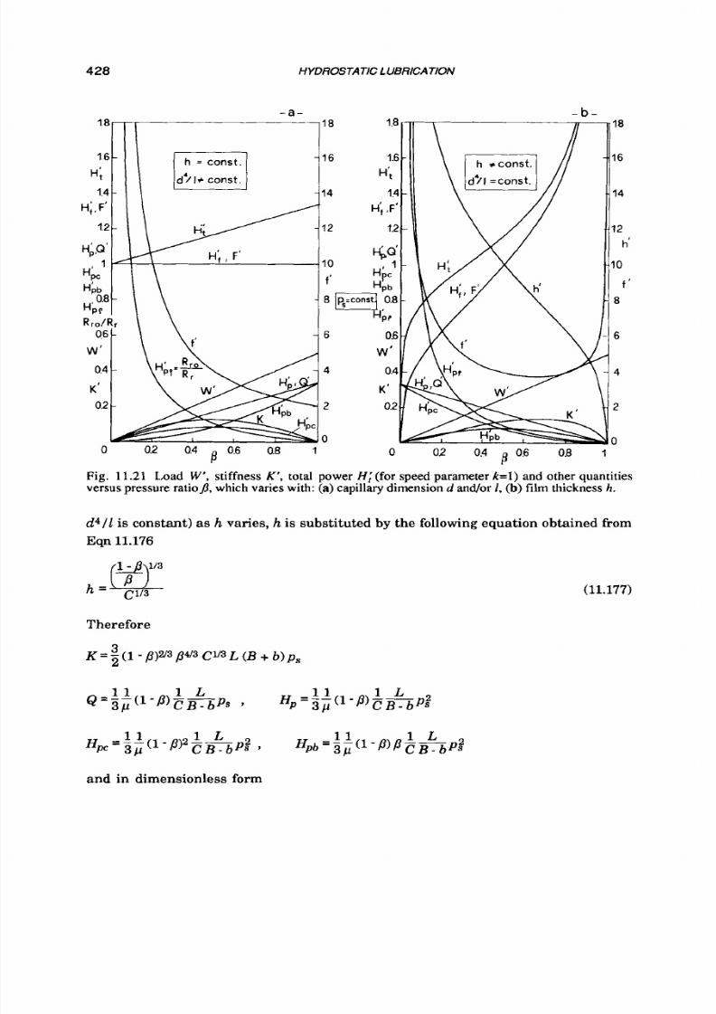
8/9/2019 Hydrostatic Lubrication 1992
http://slidepdf.com/reader/full/hydrostatic-lubrication-1992 445/558
428
1.8
-
1.6
-
H;
1.4 -
H;,F'
HpQ
H'
p"
HPb
0.8
HP,
R r o / R r
0.6
-
w
'
K '
1.2-
8 ,
1 4
0.4
-
0.2 -
HYDROSTATIC LUBRICATION
- a -
d > l +
const.
14 1
\ \1.
4
2
0
0
0.2 0.4
0.6 0.8
1
- b -
0
02
0.4
p
0.6
0.8
1
Fig. 11.21 Load W ' , stiffness
K',
total power Hi for speed parameter
k = l )
and other quantities
versus pressure ratioJ, which varies with:
(a)
capillary dimension
d
and/or I
(b)
film thickness h.
d 4 / l
is constant) as
h
vanes,
h
is substituted
by
the
following
equation obtained fiom
Eqn
11.176
(11.177)
1 1 1 L 1 1 1 L
Hpc
=
3
(1
- P I 2 empf ,
H pb =3 p
1
- P)P
c
and in dimensionless form

8/9/2019 Hydrostatic Lubrication 1992
http://slidepdf.com/reader/full/hydrostatic-lubrication-1992 446/558
429
while W' and
H i p
are identical in form to the previous ones.
The above-mentioned quantities are plotted in Fig. 11.21.b. From it, the charac-
teristics of a bearing with given dimensions, supplied at a given pressure through a
capillary tube with given dimensions, can be determined as the film (reference)
thickness varies. It must be pointed out that K is maximum for 8 = 2 / 3 (also derived
from dKldp=O) and th at for f i =0 .5 and 0.815 it is still 90% of
its
maximum value.
Therefore values of
P2O.5
up to 0.8 seem to be convenient. This is also due to the fact
that
W'
increases linearly with /3 while H P decreases linearly. Figure 11.21.b also
shows h'
from which it is possible
t o
determine h, for given bearing dimensions, capillary
tube dimensions and pressure ratio.
The performance of the bearing as a function of
L ' , b ' ,
h' and p' for any given
value of@ s still represented by Fig. 11.3.a, b, c, d, as transpires from Eqn 11.166
t o
Eqn 11.169.
11.8.2.2 Given load. In this case, which is the most frequently encountered in de-
sign, as stated earlier, p,., Q and HPb are directly given by Eqn 11.22, Eqn 11.24 and
Eqn 11.25. Furthermore
(11.178)
(11.179)
(11.180)
(11.181)
In order to investigate the performance of the pad as
varies as a consequence
of changing the dimensions of the capillary tube, as done in section 11.8.2.1, the fol-
lowing dimensionless equations can be written

8/9/2019 Hydrostatic Lubrication 1992
http://slidepdf.com/reader/full/hydrostatic-lubrication-1992 447/558
430
HYDROSTATIC
1
BRICATION
(11.182)
(11.183)
while H;,,
is
still identical in form
t o
that obtained in section 11.8.2.1.
The results are presented in Fig. 11.22.a. It must be noted that K decreases
linearly as p increases; however H i decreases as well (because H i c decreases) and
this is quite positive. Therefore, on the whole, it can be stated that intermediate
values of 8, that is /3=0.5
or
values close
to
it, are t o be adopted.
A s
for the investigation into the performance
of
the pad as
/3
varies, this time
because
h
varies, Eqn 11.177 is substituted in Eqns 11.178, 11.179, 11.180, 11.181, 11.24
and 11.25, as done in section 11.8.2.1,obtaining
K=3(1-p)2/3pu3Cv3 w
1.8
1.6
1.4
1.2
K'
1
18
1E
H't
14
H i . F;f'
1 2
H;,
10
-b-
0
02
0.4 0.6 0.8 1
B
18
1.6
I
.4
1.2
K '
1
3.8
3.6
3.4
3.2
3
Fig.
11.22
Supply pressure
p i ,
stiffness
K',
total power
H i
(for speed parameter k = l ) and other
quantities versus pressure
ratioJ,
which varies with: (a) capillary dimension d and/or
I (b)
with film
thickness
h.

8/9/2019 Hydrostatic Lubrication 1992
http://slidepdf.com/reader/full/hydrostatic-lubrication-1992 448/558
OPTlMlZATlON
431
In dimensionless form p i is still given by Eqn 11.182 while
whereas
HLp
is still identical in form to that in Eqn 11.175.
These quantities are plotted in Fig. 11.22.b. It should be noted that K is already
high when
8=0.5
nd increases further but slowly as p decreases t o /3,,=0.261; but
as decreases
HI; , Hbb
and
H i c
increase rapidly and this is quite unfavourable.
Therefore, on the whole, it can be stated that intermediate values of p , that is
p=0.5
o r values close
t o
it, are
t o
be adopted.
The performance of the bearing as a function of L', b', h' and p' is clearly still
represented in Fig. 11.4.a, b, c, d.
11.8.3 Moving
pad
11.8.3.1 Frict ion. The friction force and power are given (see section 11.5.2) by Eqn
4.49 and Eqn 11.30. They do not vary withp (Fig. 11.21.a and Fig. 11.22.a) i f i t varies
with the capillary dimensions. On the contrary they vary with /3 if
it
varies with
h
according t o Eqn 11.177. Substituting then
h
with the expression obtained from Eqn
11.177, the following dimensionless relations are obtained.
Hi.
and F j increase with j and very rapidly, too (Fig. 11.21.b and 11.22.b).
In Fig. 11.3.a, b, c, d
F i
and
H i
are plotted against
L ' , b ' ,
h' and
p '
for a given
supply pressure
p s ,
while in Fig. 11.4.a, b, c, d they are plotted for a given load W.
11.8.3.2. Friction coefficient.If the supply pressure p s is assigned, the friction coef-
ficient can be obtained by substitutingp,=/hp, in Eqn 11.37, thus
f=2-p--- 1 1 B - b
Ps
h B B + b

8/9/2019 Hydrostatic Lubrication 1992
http://slidepdf.com/reader/full/hydrostatic-lubrication-1992 449/558
432
HYDROSTATIC LUBRICATION
I fp varies with the capillary dimensions, f can be expressed as the following hnc-
tion of p
2
f ' = a
f is plotted in Fig. 11.21.a. If@varies with
h
according to Eqn 11.177, f ' can be ex-
pressed as
f ' is now plotted in Fig. 11.21.b. It is minimum forfiOpt=2/3.
If the load is assigned, f is given by Eqn 11.39. I t does not vary with p ifp vanes
with the capillary dimensions (Fig. 11.22.a). If j3 varies with h according to Eqn
11.177,f' can be written as
f ' is plotted in Fig. 11.22.b.
In Fig. 11.4.a, b, c and d,
f '
is plotted against
L',
b' , h ' and
p'.
11.8.4
11.8.4.1 Given pressure. The total power dissipated in the capillary tube and in the
moving pad is obtained by adding Eqn 11.169 to Eqn 11.30, that is
Dissipated power and ef f ic iency losses
(1 .184)
1
L
Ht
= 3 ~ p h3~ - bp U z
L
(B
-
b )
If B vanes with the dimensions of the capillary tube, with
h
then equal to a con-
stant value, Eqn 11.184 can be written, in dimensionless form, as the following func-
tion of
8:
(11.185)
H i is plotted in Fig. 11.21.a, for k=l.
I fp varies with h according to Eqn 11.176,
H i
can be expressed as the following
function of p:
8/9/2019 Hydrostatic Lubrication 1992
http://slidepdf.com/reader/full/hydrostatic-lubrication-1992 450/558
OPTIMIZATION
433
Hi is plotted in Fig. 11.21.b, for k=1.
As
a function of L',
b',
p' and c'=(1-6')p',
Hi
is again given by Eqns 11.55, 11.56,
11.61 and 11.63, respectively, p r having been replaced by p s in the expressions of k;
they have a lso been multiplied by l/$. For k= l, the curves of
H i
are presented in
Fig. 11.3.a, b and d.
The efficiency losses rk and
are still constant when they are considered to be
a fbnction of L'; they are still given by Eqn 11.65 and by the corresponding Fig. 11.6.a
and b, as a function of
6'.
Finally, as a fbnction of
h', r i
s given by Eqn 11.67 and is
plotted in Fig. 11.7.
11.8.4.2
Given
oad.
The total dissipated power is
4 1 1
W2
2-1
L
(B 6 ) (11.187)
Ht = 3 i B h 3 L ( B
6 ) ( @
-
62)
h
Ifp varies with the dimensions of the capillary tube, with
h
then equal to a con-
stant value, Eqn 11.187 can be written, in dimensionless form, a s the following hnc-
tion ofp:
Hi
is plotted in Fig. 11.22.a, for k= l .
I f p varies with
h
according to Eqn 11.176,Hi can be expressed
as
the following
function of 8:
(11.189)
Hi is plotted in Fig. 11.22.b, for k = l . It is minimum for jIoPt=0.795. Since
Popt
As a function of L',
b',
h',
p',g'=L'p' and q'=L'(l-b')p',
Hi
is again given by Eqn
11.69, Eqn 11.71, Eqn 11.73, Eqn 11.75, Eqn 11.78 and Eqn 11.81,respectively, the ex-
pressions of k having been multiplied by $. For k = l , the curves of Hi are presented
in Fig. 11.4.a, b and d.
decreases slowly as k increases, small values of p should not be adopted
$ 2 0 . 5 ) .
The efficiency loss
r i
s given, as a function of h' , by Eqn 11.83 and is plotted in
Fig. 11.8.
8/9/2019 Hydrostatic Lubrication 1992
http://slidepdf.com/reader/full/hydrostatic-lubrication-1992 451/558
434 HYDROSTATIC LUBRICA TlON
11.9 OPTIMIZATION
What
has been stated in section 11.6 still holds in general, but now the hydraulic
resistance
of
the restrictor or, better, the pressure ratio should also be considered
as an independent variable. On the other hand, it is
generally preferable to select
8
directly and treat it as a constant in the optimization process, which leads to equa-
tions that are formally identical
t o
those obtained in the case of direct supply.
As
far as the selection of
8
is concerned, the numerous remarks made in sec-
tion
6.3,
6.4.2 and 11.8 may be briefly summarized as follows:
-
from the point of view of efficiency, it is best
t o
select a high value for the pressure
ratio (perhaps
8=0.7);
-
a low value of
8
(perhaps
8=0.3)
s needed when the bearing has to sustain loads
which may considerably exceed the design value
o r
when a very high degree of
stiffness is required for any given load;
-
a value near p=0.5 is often a good compromise.
11.9.1
Given pressure
11.9.1.1
Ht=f(b,h)
11.9.1.1.1. Equation 11.184 can also be expressed as
It i s easy
to
see that the above equations are identical to those obtained in the
case of direct supply (Eqns 11.102), except that
.lisps,
is used in place of recess pres-
sure
p r .
In Fig. 11.14
Hi(b’,h’)
s plotted in the
O<b’<l
and
O<h’<2
range, for k=O.l, 1, 10.
Figure 11.16.a shows the results of the optimization of
H i ,
for OIk19, with the
constraints Osb‘s0.9 and
Och’s2 . H Im
is plotted with the corresponding optimum
values of
bbPt and h ip t; a number
of
values of hApt are also given in Table 11.2.a.
Figure 11.16 also shows
H i , Q ’
which coincides with
H i , H@
and
(11.191)
(11.192)
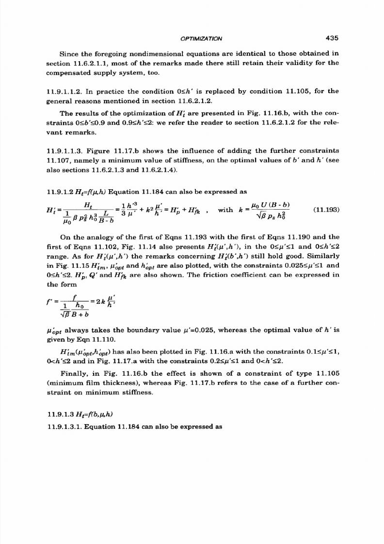
8/9/2019 Hydrostatic Lubrication 1992
http://slidepdf.com/reader/full/hydrostatic-lubrication-1992 452/558
Since the foregoing nondimensional equations are identical to those obtained in
section 11.6.2.1.1, most of the remarks made there still retain their validity for the
compensated supply system, too.
11.9.1.1.2, In practice the condition Osh'
is
replaced by condition 11.105, for the
general reasons mentioned in section 11.6.2.1.2.
The results of the optimization of Hi are presented in Fig, 11.16.b, with the con-
straints OIb'10.9 and 0.91h'<2: we refer the reader to section 11.6.2.1.2 for the rele-
vant remarks.
11.9.1.1.3. Figure 11.17.b shows the influence of adding the further constraints
11.107, namely a minimum value of stiffness, on the optimal values of b' and h' (see
also sections 11.6.2.1.3 and 11.6.2.1.4).
11.9.1.2 Ht=f(uh) Equation 11.184 can also be expressed as
On the analogy of the first
of
Eqns 11.193 with the first of Eqns 11.190 and the
first of Eqns 11.102, Fig. 11.14 also presents Hi(p',h'), in the O<p'<1 and OIh'g2
range.
A s
for H;(p',h') the remarks concerning Hi(b',h') still hold good. Similarly
in Fig. 11.15
Hirn, APt
and hAPt are also plotted, with the constraints 0.0251p'Il and
Osh'12.
Hb, Q '
and
H@
are also shown. The friction coefficient can be expressed in
the form
PApt always takes the boundary value p'=0.025, whereas the optimal value of h' is
given by Eqn 11.110.
H~rn(p~P,pt ,h~Pt)as also been plotted in Fig. 11.16.a with the constraints O.lSp'11,
k h ' a and in Fig. 11.17.a with the constraints O.21pu'11 nd 0 4 ' 1 2 .
Finally, in Fig. 11.16.b the effect is shown of a constraint of type 11.105
(minimum film thickness), whereas Fig. 11.17.b refers to the case of a fur ther con-
straint on minimum stiffness.
11.9.1.3 H&'b,b h)
11.9.1.3.1. Equation 11.184 can also be expressed
as
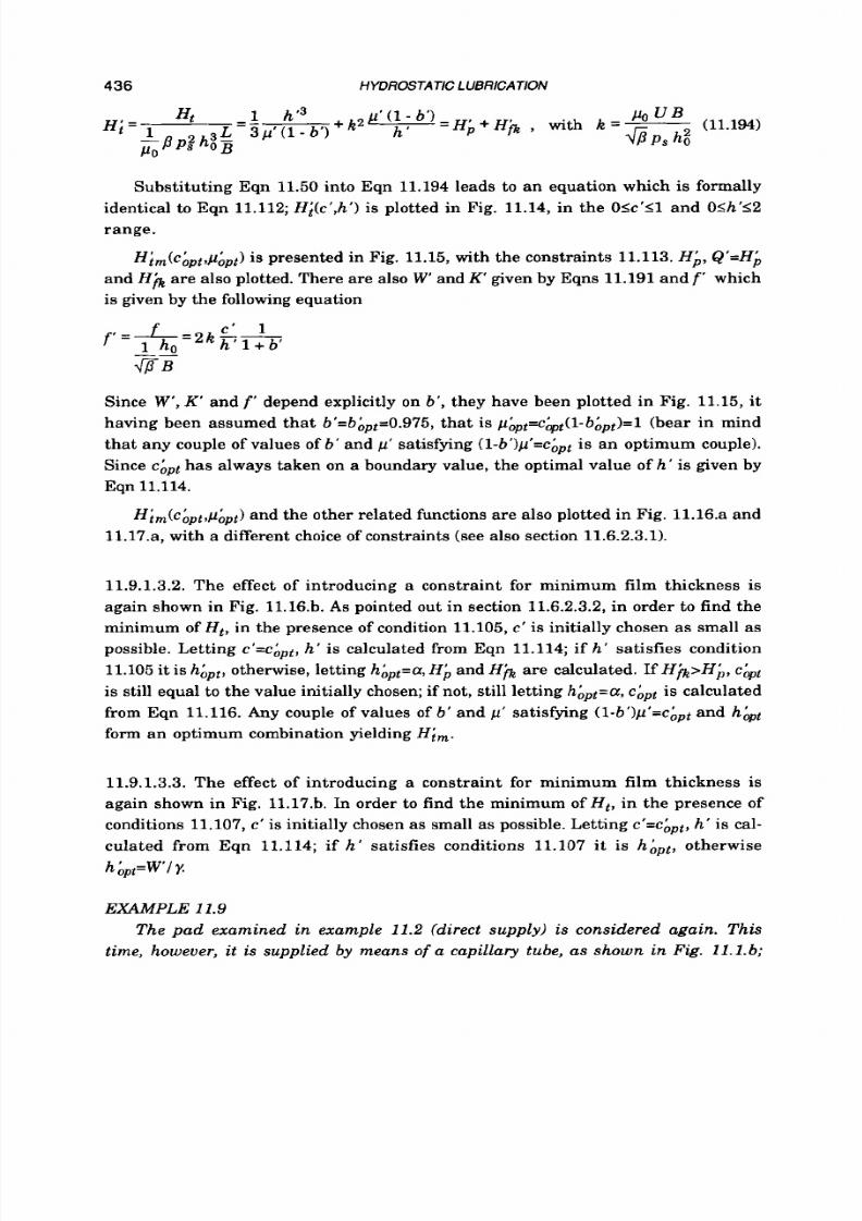
8/9/2019 Hydrostatic Lubrication 1992
http://slidepdf.com/reader/full/hydrostatic-lubrication-1992 453/558
436 HYDROSTATIC LUBRICATION
Substi tuting Eqn
11.50
into Eqn
11.194
leads
t o
an equation which
is
formally
identical to Eqn 11.112; H i(c’,h‘) is plotted in Fig. 11.14, in the O s c ‘ l l and OIh’52
range.
H ~ , ( C ~ ~ ~ , ~ & Js presented in Fig. 11.15, with the constraints 11.113. H i , Q ’ = H i
and H h are also plotted. There are also
W
and K‘ given by Eqns 11.191 and f ’ which
is given by the following equation
f ‘ = f _ = , , g r :
1 ho h l + b
_ _
4 F B
Since
W’,
K’ and f ’ depend explicitly on b‘, they have been plotted in Fig. 11.15, it
having been assumed that b’=b&=0.975, that is p ~ p t = c & l - b ~ p t ) = lbear in mind
that any couple of values of b’ and p’ satisfying ( l-b’)p’=c& is an optimum couple).
Since chpt has always taken on a boundary value, the optimal value of
h‘
is given by
Eqn 11.114.
H;m(c&&,p,pt) and the other related functions are also plotted in Fig. 11.16.a and
11.17.a, with a different choice of constraints (see also section 11.6.2.3.1).
11.9.1.3.2. The effect of introducing a constraint for minimum film thickness is
again shown in Fig. 11.16.b.
As
pointed out in section 11.6.2.3.2, in order to find the
minimum of H , , in the presence of condition 11.105, c’
is
initially chosen as small as
possible. Letting c’=c&, h‘ is calculated from Eqn 11.114; if h‘ satisfies condition
11.105 it is
h&,
otherwise, letting h&=a, H i and H @ are calculated. If H j k > H i , c&t
is still equal
t o
the value initially chosen; if not, still letting
h&,,pt=a,
&,,t is calculated
from Eqn 11.116. Any couple of values of 6’ and
p’
satisfying (l-b’)p’=c&,t and h&,t
form an optimum combination yielding
Hirn .
11.9.1.3.3. The effect of introducing a constraint for minimum film thickness is
again shown in Fig. 11.17.b. In order t o find the minimum of H , , in the presence of
conditions 11.107, c‘ is initially chosen as small as possible. Letting c’=c&, h’ is cal-
culated from Eqn 11.114; if h ’ satisfies conditions 11.107
it
is h&,, otherwise
h & = W /
EXAMPLE
11.9
T h e p a d e x am i n ed in example 11.2 (direct supply) is considered again. This
time, however, it is supplied by means of a capil lary tube, a s show n in Fig . 1 l . l .b ;
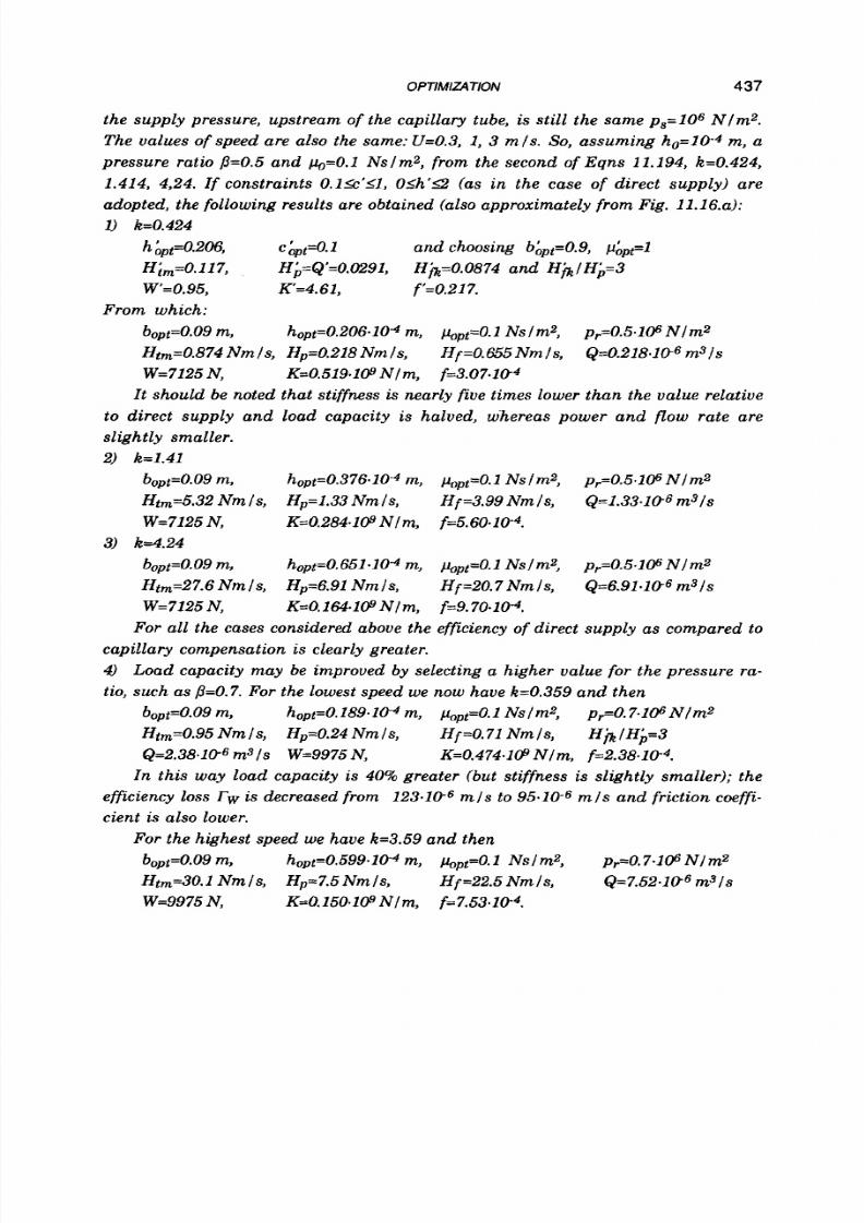
8/9/2019 Hydrostatic Lubrication 1992
http://slidepdf.com/reader/full/hydrostatic-lubrication-1992 454/558
the supply pressure, upstream of the capillary tube, is still the same ps=106 Nlm2.
The values of speed are also the same: U=0.3, I , 3 mls. So, assuming h O = l O 4 m, a
pressure ratio @=0.5and
h = O . l Nslm2, from the second of Eqns 11.194, k=0.424,
1.414, 4,24. If constraints O.le'51,
OIh'12
(as
in
the case of direct supply) are
adopted, the following results are obtained (also approximately from Fig. 11.16.a):
1) k=0.424
hbpt=0.206, c bpt=O.1 and choosing bbpt=0.9,
pAp+
Him=O.l17, Hb=Q'=0.0291,
H@=0.0874 and H@lHi=3
W=0.95, K'=4.61, f'=0.217.
From which:
bopt=0.09m, hopt=0.206.10-4m, kPt=O.1Nslmz, p,=0.5.106 Nlm2
Htm=O.874 Nmls, Hp=0,218Nmls, Hf=0.655Nmls, Q=0.218.106 m3/s
W=7125N, K=0.519.109 N
1
m, f=3.07.1@4
It should be noted that stiffness is nearly five times lower than the value relative
to
direct supply and load capacity is halved, wAereas power and flow rate are
slightly smaller.
2) k=1.41
bopt=0.09m, hopt=0.376. 0-4 rn, popt=O.1 NsIm2, pr=0.5.1
06
N Im2
HtmS.32 N m s, Hp=1.33N m
s ,
Hfd.99 Nmls, &=1.33.106 m3 /s
W=7125N, K=0.284.109 Nlm, f=5.60.10-4.
bopt=0.09m, hopt=0.651.10-4m, kpt=0.l NsIm2, p,=0.5.106 Nlm2
Htm=27.6 Nmls, Hp=6.91Nmls , Hf=20.7 Nmls , &=6.91.1@6 m3/s
W=7125N, K=O. 164.1
09
N 1m, f=9.70.10-4.
3) kd.24
For all the cases considered above the efficiency of direct supply as compared to
capillary compensation
is
clearly greater.
4) Load capacity may be improved by selecting a higher value for the pressure ra-
tio, such as p=O.7. For the lowest speed we now have k=0.359 and then
bopt=0.09
n,
hopt=0.189.10-4m, popt=O.l Nslm2, pr=0.7-106Nlm2
Htm=O.95 Nmls, Hp=0.24 Nmls, Hf=O.71Nmls, H@lHb=3
Q=2.38.106 m3Is
W=9975N, K=0.474.108 Nlm, f=2.38.104.
In this way load capacity is 40% greater (but stiffness is slightly smaller); the
efficiency loss rw is decreased from 123.106 m l s to 95.10-6 ml s and friction coeffi-
cient is also lower.
For the highest speed
we
have k=3.59 and then
bopt=0.09m, hopt=0.599.10-4m, kpt=0.l Nslm2, p,=0.7.106 Nlm2
Htm=30.1 Nmls, Hp=7.5Nmls , Hf'22.5 Nmls , Q=7.52.106 mats
W=9975N, K=O. 150.109 N l m, f = 7.53-104.

8/9/2019 Hydrostatic Lubrication 1992
http://slidepdf.com/reader/full/hydrostatic-lubrication-1992 455/558
438
HYDROSTATIC LUBRICA
TlON
11.9.2 Given
load
11.9.2.1 Ht=f(b,h)
11.9.2.1.1. Equation 11.187 can be also expressed as
(11.195)
The analogy with Eqn 11.117 is clear. In Fig. 11.18 Hi(b',h') is plotted in the
Ogb'll
and Osh'12 range, for k=0.1,
1,
10. What has been said
in
section 11.6.3.1.1, concern-
ing Fig. 11.18, still holds good.
Figure 11.19.a shows the results of the optimization of Hi, for OIkI6, with the
constraints Osb's0.9 and Osh's2.
Him
is plotted with the corresponding optimum
values of bApt and h& H@and
H ;
are also plotted, as well as p; (given by the first of
Eqns 11.1181,
Q'
(given by the first of Eqns 11.119) and
(11.196)
(1
.197)
It should be noted that, as in the case of direct supply, bApt has always taken the
boundary value b'=0.9; therefore hAPt can be determined from Eqn 11.120.
11.9.2.1.2. In practice the condition Osh' is substituted with condition 11.105 for the
reasons mentioned in section 11.9.1.1.1. The results of the optimization of Hi, with
the constraints Od~'10.9,0.61h'<2, are presented in Fig. 11.19.b (see section
11.6.3.1.2 for the relevant remarks).
For the optimization with assigned load and constraint 11.105, bAPt is initially
chosen as large as possible, and h ' is calculated by means of Eqn 11.120. Then,
if
constraint 11.105 is satisfied, such a value of h' is the optimum one; otherwise,
a
s
chosen as hhpt and
bhPt
is calculated from Eqns 11.72
(or
Fig. 11.4.b) in which
(1 .198)
If, on the other hand, the value of
b'
thus calculated is greater than the upper limit
selected for b', the latter has to be chosen as
bhPt.

8/9/2019 Hydrostatic Lubrication 1992
http://slidepdf.com/reader/full/hydrostatic-lubrication-1992 456/558
OPTlMlzATION
439
11.9.2.1.3. For high values of k the above procedure may lead
t o
a high film thick-
ness and, hence, to poor stiffness. In the presence of constraints 11.122 on mini-
mum stiffness the optimization procedure should be modified as follows: the upper
limit of
b '
is firstly selected as
bApt
and h ' is calculated from Eqn 11.120. If con-
straints 11.122 ar e not satisfied, i t must be assumed that
h&=l/y.
11.9.2.2 H,=f(Uh) Equation 11.187 can also be expressed as
(11.199)
The nondimensional coefficients
p i , p i
and K can still be calculated by means of
Eqns 11.196, whereas for Q' and
f '
we have:
Optimization may be performed choosing the lowest available viscosity and
calculating h& from Eqn 11.124.
As
usual, for small values of
k ,
film thickness will
be too low; in this case, in the presence of constraint 11.105, we shall assume h&=a
and calculate p& from Eqn 11.125.
11.9.2.3 H,=f&,h) Equation 11.187 can also be expressed
as
The considerations regarding Eqn 11.199 are still valid, if only p ' is replaced by L'.
11.9.2.4 H,=f(L,p,h) Equation 11.187 can also be expressed as
(1 .201)
If
we substitute Eqn 11.77 into Eqn 11.201,
it
becomes
(11.202)
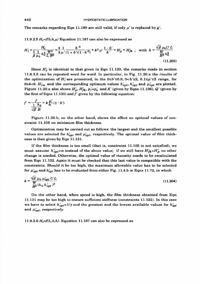
8/9/2019 Hydrostatic Lubrication 1992
http://slidepdf.com/reader/full/hydrostatic-lubrication-1992 457/558
440 HYDROSTATIC LUBRICATION
The remarks regarding Eqn 11.199 are still valid, if only
p'
is replaced byg'.
11.9.2.5H,=flb,h,p) Equation 11.187 can also be expressed as
(11.203)
Since HI is identical to that given in Eqn 11.129, the remarks made in section
11.6.3.5 can be repeated word for word. In particular, in Fig. 11.20.a the results
of
the optimization of
HI
are presented, in the O<b'10.9,Och'12, O.1<p1'S2 ange, for
O<k<6.
Him
and the corresponding optimum values
bhpt,
hhpt and
pbpt
are plotted.
Figure 11.20.a also shows Hb, H@,p;=p; andK' (given by Eqns 11.1961,
Q'
(given by
the first of Eqns 11.130) and f given by the following equation:
-f k
$ 1
6')
f - 1 ho
Figure 11.20.b, on the other hand, shows the effect on optimal values of con-
straint 11.105 on minimum film thickness.
Optimization may be carried out as follows: the largest and the smallest possible
values are selected for bhpt and p&, respectively. The optimal value
of
film thick-
ness is then given by Eqn 11.131.
If the film thickness is too small (that is, constraint 11.105 is not satisfied), we
must assume h&a instead of the above value; if we still have H@>Hbno other
change is needed. Otherwise, the optimal value of viscosity needs to be recalculated
from Eqn 11.132. Again it must be checked that this last value is compatible with the
constraints. Should
it
be too high, the maximum allowable value has to be selected
for
p&
and
b& has
t o
be evaluated from either Fig. 11.4.b
or
Eqns 11.72, in which
(11.204)
On the other hand, when speed is high, the film thickness obtained from Eqn
11.131may be too high to ensure sufficient stiffness (constraints 11.122). In this case
we have to select h&,,pt=llyand he greatest and the lowest available values for b&
and
p&,
respectively.
11.9.2.6 H,=f(L,b,h). Equation 11.187 can also be expressed as
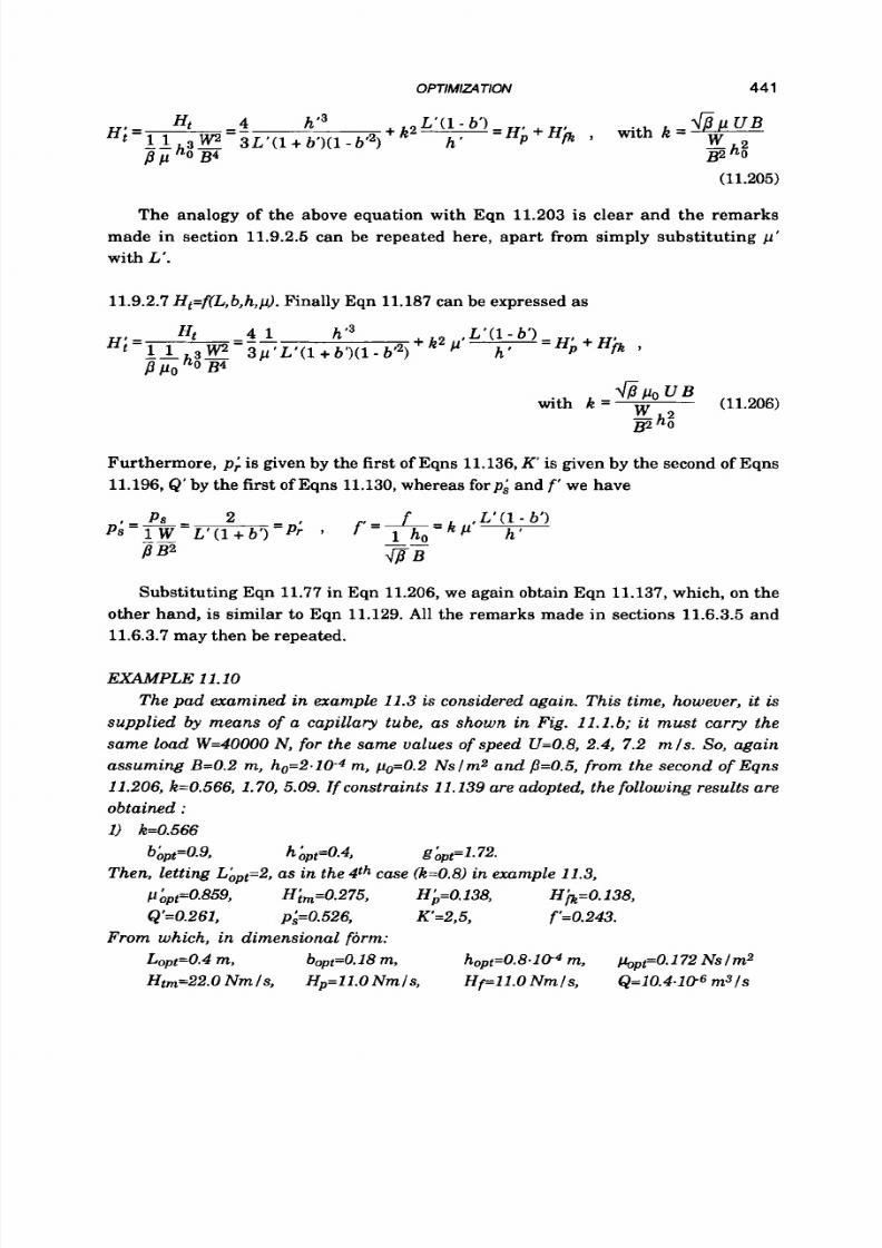
8/9/2019 Hydrostatic Lubrication 1992
http://slidepdf.com/reader/full/hydrostatic-lubrication-1992 458/558
OPTIMIZ4TION
441
(11.205)
The analogy of the above equation with Eqn 11.203 is clear and the remarks
made in section 11.9.2.5 can be repeated here, apart from simply substituting
p'
with L'.
11.9.2.7 H,=f(L,b,h,p). Finally Eqn 11.187 can be expressed as
(11.206)
PO U B
with k =
Furthermore, p;
is
given by the first of Eqns 11.136,K
is
given by the second of Eqns
11.196, Q' by the
first
of Eqns 11.130,whereas forpi and
f
we have
Substituting Eqn 11.77 in Eqn 11.206,we again obtain Eqn 11.137, which, on the
other hand, is similar to Eqn 11.129. All the remarks made in sections 11.6.3.5 and
11.6.3.7 may then be repeated.
EXAMPLE 11.10
The pad examined in example 11.3 is considered again. This time, however, it is
supplied by means of a capillary tube, as shown in Fig. 11.1.6; it
must
carry the
same load W=40000 N, for the same values
of
speed U=0.8, 2.4,
7.2
mls.
So,
again
assuming B=0.2 m, ho=2.10-4m, &=0.2 Nslm2 and P=0.5, from the second of Eqns
11.206, k=0.566, 1.70, 5.09. I f constraints 11.139 are adopted, the following results are
obtained :
1) k=0.566
Then, letting LApt=2,as in the 4th case (k=O.8)in example 11.3,
bAp,pt=0.9, h Ap,pt=0.4, gAp,pt=l.2.
~Ap,t=O.859, Him=0.275, Hi=O.138, Hb=O.138,
Q'=0.261, pi=0.526, K=2,5, f'=0.243.
Lapt=0.4m, bapt=0.18m, hapt=0.8.104
m,
hpt=0.172 Nslm2
Htm=22.0 NmJs , Hp=ll.ONmls , Hp11.0 Nmls , Q=10.4.10-6 m3/s
From which,
in dimensional form:

8/9/2019 Hydrostatic Lubrication 1992
http://slidepdf.com/reader/full/hydrostatic-lubrication-1992 459/558
4 4 2 HYDROSTATE
L
UBRlCATloN
p,=1.05.106 Nlm2, p,.=0.526.106 Nlm2, K=7.50.1@ Nlm, f=3.44.104.
Comparing the above values with those obtained
in
the fourth case in example
11.3 (direct supply), it may be noted that stiffness is halved, supply pressure is dou-
bled and power is 32% greater.
2) k=1.7
example 11.3,
Letting now LApt=l and using constraints 11.138, as in the second case in
Lopt=0.2m,
bopt=0.18m, hOpt=0.254.1O4 , kpt=0.02Nslm2
Htm=24.2 N m Is,
Hp=6.1Nm s, Hp18.1 Nmls, Q=2.87.1Q6 m31s
ps=2.10.106 N
1
m2, p,=1.05.106 N l m2,
K=23.6-1@N l m, f=l.89.104.
Compared to the second case in example 11.3, Htm is 20% greater and supply
pressure is doubled, whereas K is 40% lower. Moreover these results require a film
thickness which
is
notably smaller. If the same
f i lm
thickness as in example 10.3
(case 2) were used, stiffness would be further reduced.
3) kd .09
Again letting LAPt=l,as in the third case in example 11.3,
LOpt=0.2m,
bopt=O. 18m, hopt=0.440-104m, kpt=0.02 Nslmz
Htm=126Nmls,
Hp=31.4 Nm ts , Hp94.3 Nml s, Q=14.9.106 m3ts
p,=2.10.106 Nlm2,
p,=1.05.106 Nlm2, K=13.6.108 Nlm, f=3.27.104.
4) In all three cases stiffness is clearly lower than in the case of the pad which is
directly supplied, in spite of the smaller values of optimal f ilm thickness. I t should
be noted that the only way to improve stiffness (apart the obvious solutions of further
reducing clearance
or
increasing load) is to reduce p. In reference to the first case,
still letting L=0.4 m and h'20.4, the following results are obtained, now for p=0.3
(that
is
k =0.438):
bApt=0.89, h Ap,pt=0.4,
g
Apt'2.
From
which, in dimensional form:
Lopt=0.4m,
bopt=O. 79 m, hopt=0.8-104m, kpt=0.2Nslm2
Htm=28.5 Nmls,
Hp=15.0Nm ls , Hp13.5 Nml s, Q=8.55.106 m31s
p,=l.76.106 Ntm2, p,=0.528.106 Nlm2, K=10.5.1@ Nlm, f=4.2-104.
It is clear than the 40% increase in stiffness has been paid for with a notable
increase in power and supply pressure. Compared with the fourth case in example
11.3, K is still much lower, even though Htm is now much higher. A further de-
crease in pressure ratio would lead to a higher stiffness (although the stiffness of
the pad that is directly supplied cannot be reached anyway), but with very high val-
ues
of
supply pressure and power consumption. For instance, for
p=O. l
we would
obtain:
Lopt=0.4 m, bopt=O. 63 m, hopt=0.8. 04 m, kpt=0.2Ns Im2
Htm=51.7 Nm S, Hp=28.3Nmts , Hr23 .4 Nmls , Q=5.14-1O6 m31s
ps=5. 0-106N Im2, p,,=0.550.106 N l
m2,
K=13.5.1OB N Im,
f = 7.3.104.
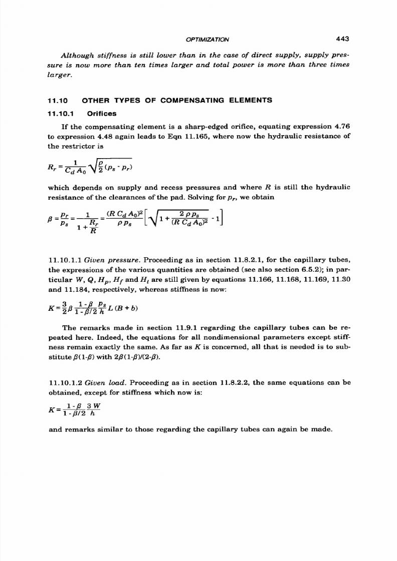
8/9/2019 Hydrostatic Lubrication 1992
http://slidepdf.com/reader/full/hydrostatic-lubrication-1992 460/558
OPTlMlZ4
TlON
443
Althoug h stiffnes s is still lower than in the case of direct su pply, sup ply pres -
sure is now more than ten times larger and total power is more than three times
larger .
11.10
OTHER
TYPES
OF
COMPENSATING ELEMENTS
11.10.1
Orif ices
If the compensating element is a sharp-edged orifice, equating expression 4.76
t o expression 4.48 again leads t o Eqn 11.165, where now the hydraulic resistance of
the restrictor is
which depends on supply and recess pressures and where R is still the hydraulic
resistance of the clearances of the pad. Solving for p, , we obtain
11.10.1.1
Given pressure.
Proceeding as in section 11.8.2.1, for the capillary tubes,
the expressions of the various quantities are obtained (see also section
6.5.2);
in par-
ticular
W, &, H p , H f
andHt are still given by equations
11.166, 11.168, 11.169, 11.30
and
11.184,
respectively, whereas stiffness is now:
The remarks made in section 11.9.1 regarding the capillary tubes can be re-
peated here. Indeed, the equations
for
all nondimensional parameters except stiff-
ness remain exactly the same.
As
far as R is concerned, all that is needed is to sub-
stitute P(1-p)with 2P(l-p)/(2-p).
11.10.1.2 Given load. Proceeding as in section 11.8.2.2, the same equations can be
obtained, except for stiffness which now is:
and remarks similar t o those regarding the capillary tubes can again be made.

8/9/2019 Hydrostatic Lubrication 1992
http://slidepdf.com/reader/full/hydrostatic-lubrication-1992 461/558
4 4 4
HYDROSTATlC L UBRlCATlON
11.10.2 Flow-cont ro l va lves
If the compensating element is a flow-control valve, the flow-rate Q through the
pad is constant. The hydraulic resistance of the restrictor must hence be
where R is the hydraulic resistance of the pad. Thus
11.10.2.1 Given pressure.
Proceeding as in section
11.8.2.1
the expressions of the
various quantities are obtained (see also section
6.5.3);
in particular Eqn
11.166
and
all the equations from 11.168
to
11.172 are still valid, as well
as
Eqn 11.184, whereas
stiffness
is
now
The remarks made in section 11.9.1 regarding the capillary tubes can be re-
peated here. Indeed, the equations
for
all nondimensional parameters except stiff-
ness remain exactly the same.
As
far as
K
is concerned, all that is needed is
to
sub-
stitute p(1-PIwith
p.
11.10.2.2 Given load. Proceeding as in section 11.8.2.2,we can obtain again the same
equations, except for stiffness which is now given by Eqn 11.23: namely, i t is identi-
cal to th at obtained in the case of direct supply (naturally, within the operating
range of the valve).
As
regards the operating range, the smaller
P
is, the wider the
operating range is, as shown in Fig.
6.10.
11.11 REAL
PADS
The formulae of the total power for the infinite pad in the case of compensated
supply differ from those of the directly supplied pad for p, . replaced by @ps in the
case of constant pressure, and for
W
replaced by W I G n the case of constant load.
As for the rest they are unchanged.
This
also
holds good for the other types of pad: rectangular, circular and annu-
lar, the formulae of which are the following:
Eqns 11.149and 11.152for the rectangular pad,
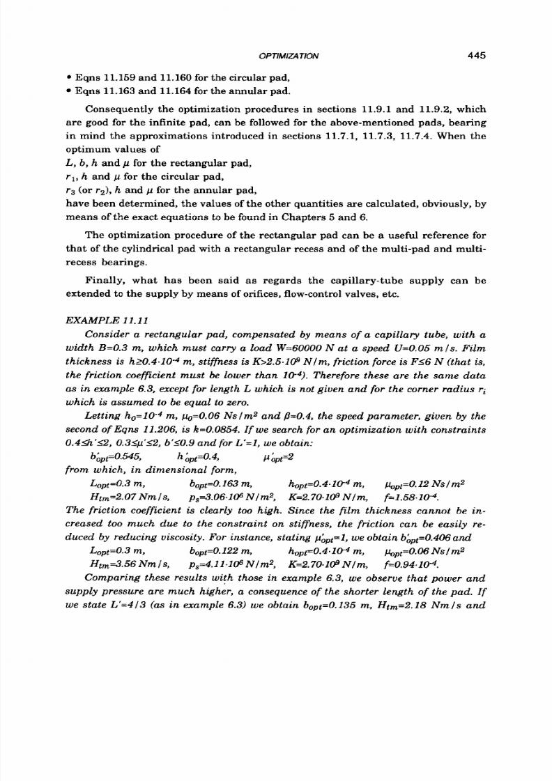
8/9/2019 Hydrostatic Lubrication 1992
http://slidepdf.com/reader/full/hydrostatic-lubrication-1992 462/558
OPTlMlZATlON
445
Eqns 11.159 and 11.160 for the circular pad,
Eqns 11.163 and 11.164 for the annular pad.
Consequently the optimization procedures in sections
11.9.1
and
11.9.2,
which
are good for the infinite pad, can be followed
for
the above-mentioned pads, bearing
in mind the approximations introduced in sections
11.7.1, 11.7.3, 11.7.4.
When the
optimum values of
L, b ,h
and p for the rectangular pad,
rl, h
and p
for
the circular pad,
r3 (or r z ) ,
h
and p for the annular pad,
have been determined, the values of the other quantities ar e calculated, obviously, by
means of he exact equations to be found in Chapters 5 and 6.
The optimization procedure of the rectangular pad can be a useful reference for
that of the cylindrical pad with a rectangular recess and of the multi-pad and multi-
recess bearings.
Finally, what has been said as regards the capillary-tube supply can be
extended t o the supply by means of orifices, flow-control valves, etc.
EXAMPLE 11.11
Consider a rectangular pad, compensated by means o f a capillary tube, with a
width
3=0.3
m, which must carry a load
W=60000
N at a speed U=0.05ml s. Film
thickness is h20.4.104
m,
stiffness is K>2.5.1@ Nlm, friction force is
F 1 6
N (that is,
the friction coefficient must be lower than 10-4). Therefore these are the same data
as in example 6.3, except for length
L
which is not given and for the corner radius
ri
which is assumed to be equal to zero.
Letting ho=104m,
&=0.06
Nslm2 and 8=0.4, the speed parameter, given by the
second of Eqns 11.206, is k=0.0854.
I f
we search for an optimization with constraints
0.4&'12, 0.35pr52,b'10.9 and for L'=l, we obtain:
from which, in dimensional form,
bhp,pt=0.545, h APt=0.4,
P
Apt*
Lopt=0.3m, bopt=0.163m, hopt=0.4-104m, kpt=0.12Nslm2
Htm=2.07 Nmls, p,=3.06*106 Nlm2, K=2.70*1@Nlm, f=1.58.104.
The friction coefficient is clearly
too
high. Since the film thickness cannot be in-
creased too much due to the constraint on stiffness, the friction can be easily re-
duced by reducing viscosity. For instance, stating pApt=l,we obtain bApt=0.406and
Lopt=0.3m, bopt=0.122m,
hopt=0.4.104m, kpt=0.O6Nsl m2
Htm=3.56Nmls, p,=4.11.106 Nlm2, K=2.70.1@ Nlm,
f=0.94.104.
Comparing these results with those in example 6.3,
we
observe that power and
supply pressure are much higher, a consequence of the shorter length of the pad. I f
we state L'=4/3 (as in example 6.3) we obtain bopt=0.135 m, Htm=2.18 N m l s and
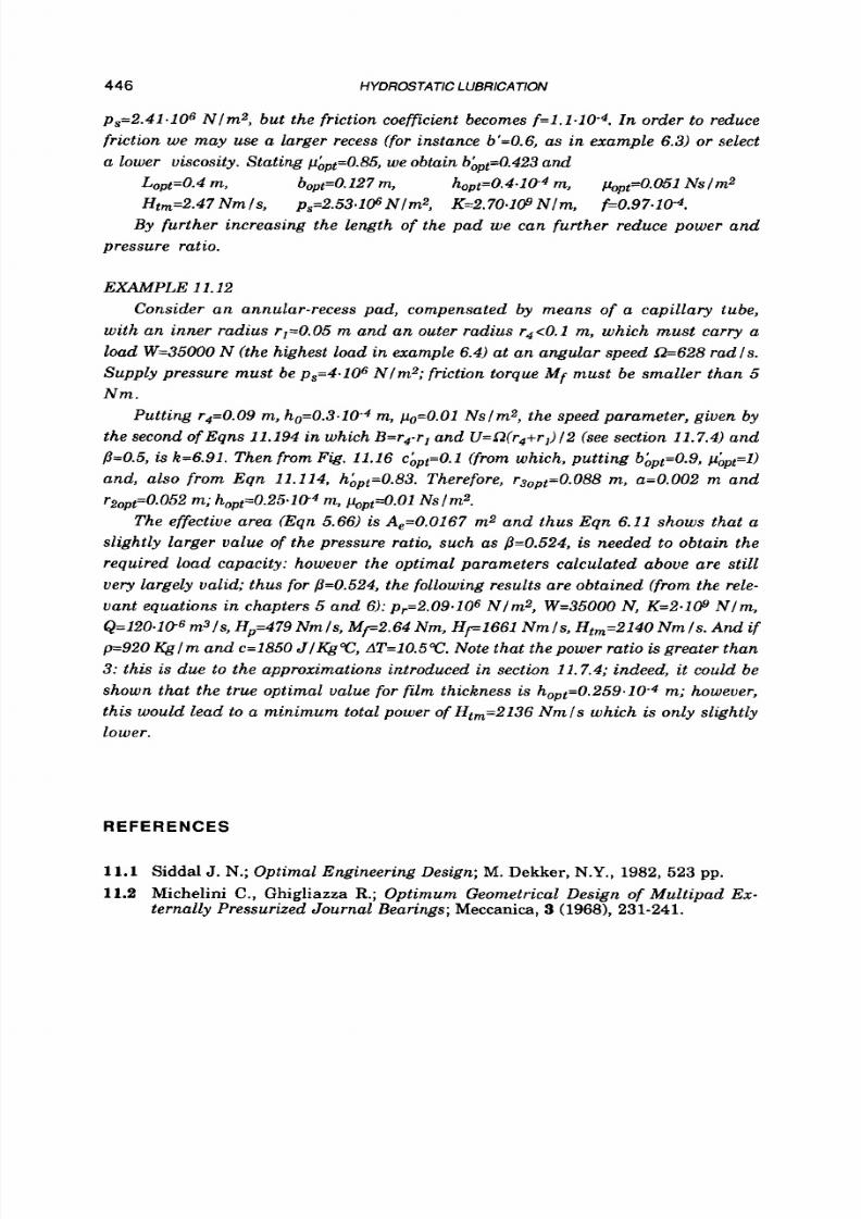
8/9/2019 Hydrostatic Lubrication 1992
http://slidepdf.com/reader/full/hydrostatic-lubrication-1992 463/558
446
HYDROSTATIC 1UBRlCATlON
p,=2.4l.1O6 Nlm2, but the friction coefficient becomes f = l . l . l O - 4 . In order to reduce
friction we may use a larger recess (for instance b'=0.6, as in example 6.3)
or
select
a lower viscosity. Stating pApt=0.85,we obtain bApt=0.423and
Lopt=0.4m, bopt=0.127m, hopt=0.4.1f34m,
hpt=0.051
slm2
Htm=2.47 Nmls, p,=2.53.106 Nlmz,
K=2.70.1@ Nlm, f=0.97.10 1.
By further increasing the length of the pad we can further reduce power and
pressure ratio.
EXAMPLE 11.12
Consider an annular-recess pad, compensated by means of a capillary tube,
with an inner radius r,=0.05 m and an outer radius r4<0.1
m,
which must carry a
load W=35000N (the highest load in example 6.4) at an angular speed Q=628 rad
Is .
Supply pressure must be p,=4.lO6 Nlm2; friction torque Mf must be smaller than 5
N m .
Putting r4=0.09 m, ho=0.3.104 m, h = O . O l Nslm2, the speed parameter, given by
the second ofEqns 11.194 in which B=r4-rl and U=R(r4+rl)12 see section 11.7.4) and
8=0.5,
s k=6.91. Then from Fig. 11.16
C ~ ~ ~ = O . ~
from which, putt ing bApt=0.9, pAPt=l)
and, also from Eqn 11.114,
h&=0.83.
Therefore,
r30pt=0.088
m, a=0.002 m and
rzopt=O.052m; hOpt=0.25.1O4 ,
,pt=O.Ol
Ns
Im2.
The effective area (Eqn 5.66) is A,=0.0167 m2 and thus Eqn 6.11 shows that a
slightly larger value of the pressure ratio, such as 8=0.524, is needed to obtain the
required load capacity: however the optimal parameters calculated above are still
very
largely valid; thus for 8=0.524, the following results are obtained (from the rele-
vant equations in chapters 5 and 6): p,=2.O9.1O6 Nlm2, W=35000 N, K=2.109 Nlm ,
Q=120.106 m3/s, Hp=479Nmls, M ~ 2 . 6 4 m, Hf=1661Nm ls , Ht,=2140 Nmls . And i f
p=920Kg/mand c=1850JI IQC, AT=10.5%. Note that the power ratio isgreater than
3: this is due to the approximations introduced in section 11.7.4; indeed, i t could be
shown that the true optimal value for fi lm thickness is hOpt=0.259.10-4m; however,
this would lead to a min imum total power of Htm=2136 N m / s which is only slightly
lower.
R E F E R E N C E S
11.1
Siddal J. N.; Optimal Engineering Design; M. Dekker, N.Y.,
1982,
523
pp.
11.2
Michelini C., Ghigliazza R.; Optimum Geometrical Design of Multipad Ex-
ternally Pressurized Journal Bearings;
Meccanica,
3
(19681, 231-241.

8/9/2019 Hydrostatic Lubrication 1992
http://slidepdf.com/reader/full/hydrostatic-lubrication-1992 464/558
Chapter 12
THERMAL FLOW
12.1 INTRODUCTION
In the previous chapters, all the heat produced in the lubricant of hydrostatic
bearings by friction from viscous drag was assumed to remain in the lubricant itself
(adiabatic flow).
In this chapter the thermal flow in a hydrostatic system is studied, taking into
account heat transfer by the various parts: bearing, supply pump, compensating
element, and
so
on, showing how cooling can occur especially in the supply
pipelines and in the reservoir, provided that they are suitably dimensioned.
12.2 TEMPERATURES IN THE BEARING
12.2.1 Temperatures
in
the film
As
already seen, with the assumption
of
adiabatic flow, the elementary rela-
tionship
5.7
holds good, but a further analysis involves the introduction of the en-
ergy equation
4.37
n the mathematical model, as happens in ref.
5.14
in the case of
the circular pad, assuming known temperatures on the facing surfaces (ref.
5.15).
In this chapter the thermal flow in another elementary pad is studied: the in-
finitely long hydrostatic pad in Fig.
11.1, of
width
B,
recess width b and of which a
finite part of length L
is
considered. The mathematical model is quite simple (ref.
12.1),
f the variation of viscosity with temperature is disregarded, a s in this case.
On the other hand, heat transfer between lubricant, pad and ambient is not
disregarded.
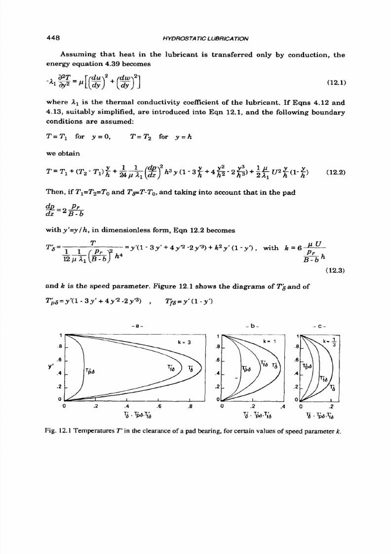
8/9/2019 Hydrostatic Lubrication 1992
http://slidepdf.com/reader/full/hydrostatic-lubrication-1992 465/558
448 HYDROSTATIC LUBRICATION
Assuming that heat in the lubricant
is
transferred only by conduction, the
energy equation 4.39 becomes
(12.1)
where Al is the thermal conductivity coefficient of the lubricant.
If
Eqns
4.12
and
4.13,
suitably simplified, are introduced into Eqn
12.1,
and the following boundary
conditions are assumed:
T=T, for y=O, T=T2 for y = h
we obtain
Then, if Tl=T2=Tond Td=T-T0, nd taking into account that in the pad
with y'=y
I
h, in dimensionless form, Eqn 12.2 becomes
(12.3)
and k
is
the speed parameter. Figure 12.1 shows the diagrams of Tiand of
T i a = y ' ( l -
~ ' + 4 ~ ' 2 - 2 ~ ' 3 ) Tja=y'(l -y')
- a - -
b -
- c -
0
.2
.4 .6 .8 0 .2 .4
0
.2
T i , T+T& T i
I
ThqT;d
T i I
,Ti&
Fig. 12.1
TemperaturesT' n the clearance
of
a pad bearing, or certain values
of
speed parameter k.

8/9/2019 Hydrostatic Lubrication 1992
http://slidepdf.com/reader/full/hydrostatic-lubrication-1992 466/558
THERMAL
FLOW
449
for k=1/3, 1, 3. As far as the intermediate case is concerned, it should be noted that,
even if Hp=Hf for k = l , Ths s always smaller than Ti8 because of the different pat-
terns of
u
and w , he former being linear, the latter parabolic. This still holds good
for
k=1/3
and obviously for
k=3,
too.
The diagrams in Fig. 12.1 partly correspond to those in Fig.
5.10,
obtained by
numerical analysis for the circular pad, without the simplifying assumptions of
Eqn 4.39.
As may be seen in
Fig.
5.10, which also takes into account the variation of vis-
cosity with temperature, the average temperature of the lubricant increases
(virtually linear) with the radius of the circular pad. Consequently the average
temperature of the film may be assumed to increase with
z
while this cannot be
established from Eqn
12.3.
As
a h r ther approximation the temperature
at
the film
inlet, where
w=O
(see section 4.8 for what concerns the "inlet length), is assumed
t o
be equal to TFs.
12.2.2 Temperatures at
the
f i lm out let
Naturally the temperature variation in the lubricant is related to the heat en-
ergy transferred &om i t to the pad and then to the ambient. The phenomenon can be
described briefly as follows.
H t
is
the total power dissipated because of friction from viscous drag in the film
(it is assumed to be equal
t o
zero in the recess), H , and H s are the heat energies
transferred between the lubricant and the pad in the recess and in the film, respec-
tively;
T,
nd T, are the temperatures a t the recess inlet and at the film outlet,
re-
spectively (Fig.
12.2).
Then
(12.4)
On the other hand, using Ti to denote the temperature at the film inlet and
Tr
and Fs t o indicate the average temperatures in the recess and in the film, respec-
tively, and putting
- T,. + Ti Ti + T,
T,.
- 2 1 Ts=- 2
(12.5)
we have
(12.6)
where

8/9/2019 Hydrostatic Lubrication 1992
http://slidepdf.com/reader/full/hydrostatic-lubrication-1992 467/558
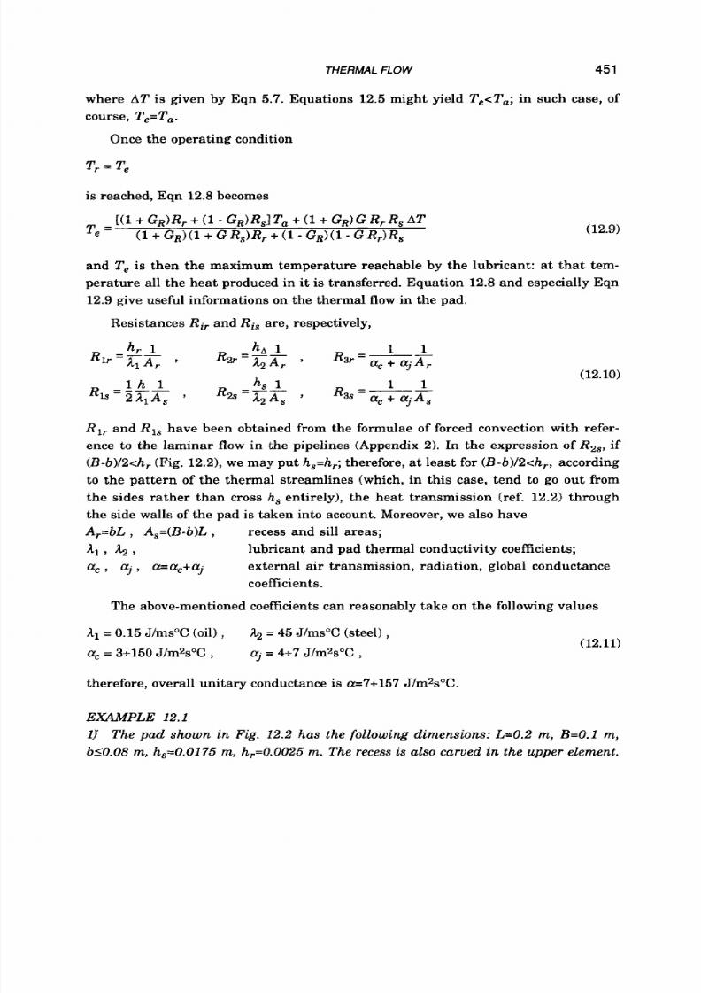
8/9/2019 Hydrostatic Lubrication 1992
http://slidepdf.com/reader/full/hydrostatic-lubrication-1992 468/558
THERMAL FlOW 45 1
where
AT
is given by Eqn
5.7.
Equations
12.5
might yield
Te<Ta;
n such case, of
course, Te=Ta.
Once the operating condition
T,
= Te
is reached, Eqn 12.8 becomes
[ ( ~ + G R ) R , + ( ~ - G ~ ) R , ] T ~ + ( ~ + G ~ ) G R , R , A T
T , = ( l + G ~ ) ( l + G R s ) R , + ( l - G ~ ) ( l - G R r ) R s
(12.9)
and T , is then the maximum temperature reachable by the lubricant: a t that tem-
perature all the heat produced in i t is transferred. Equation 12.8 and especially Eqn
12.9
give useful informations on the thermal flow in the pad.
Resistances Ri, and Ri, are, respectively,
(12.10)
R1,
and R1, have been obtained from the formulae of forced convection with refer-
ence
t o
the laminar flow in the pipelines (Appendix
21.
In the expression of
Rzs,
if
(B-b)/2<h,
Fig.
12.21,
we may put
h,=h,;
therefore, a t least for
(B-b)/2chr,
according
t o the pattern of the thermal streamlines (which, in this case, tend
to
go out from
the sides rather than cross h, entirely), the heat transmission (ref.
12.2)
through
the side walls of the pad is taken into account. Moreover, we also have
A,=bL
,
A,=(B-b)L ) recess and sill areas;
2 1 3 2 9
ac aj
, a=ac+aj
external air transmission, radiation, global conductance
lubricant and pad thermal conductivity coefficients;
coefficients.
The above-mentioned coefficients can reasonably take on the following values
A1 = 0.15 J/ms°C (oil ),
ac=
3+150
J/m2s°C,
& = 45 J/ms°C (steel) ,
a j
= 4*7
J/m2soC
therefore, overall unitary conductance is
a=7+157
J/m2soC.
(12.11)
EXAMPLE 12.1
11 The pad shown in
Fig.
12.2 has the following dimensions: L=0.2
m,
B=O.l
m,
b10.08 m, h,=0.0175 m, h,=0.0025 m. The recess is also carved in the upper element.

8/9/2019 Hydrostatic Lubrication 1992
http://slidepdf.com/reader/full/hydrostatic-lubrication-1992 469/558
452 HYDROSTATIC LUBRICATION
The bearing operating conditions are W=31180 N, U=8.66ml s , and the lubricant
properties are: p=0.025 Ns I
m2,
p 8 9 7
Kg
m3, c=1930J I Kg
"y:
(at 35"c).
According to what has been specified in section 11.6.3.1.1, we put bAPt equal to
0.8,
thus bOpt=0.08
m
and putting the reference value ho=104
m,
the second of Eqns
11.73yields k=0.144 which substituted in Eqn 11.74 yields
hhpt=0.5, hus hOpt=0.5.10-4m. Moreover
p,=1.73.106 Nlm2, Q=28.9.10-6 m3/s, Hp=50 NmIs, F=17.3 N , Hf=150 NmI s, Ht=200
N m / s , HflHp=3, K=1.87.109 Nl m , f=5.5.10-4. Then, from Eqn 5.7, AT=4"C. These
values are given in Table 12.1, together with those obtained in the same conditions
but for other values of
U.
'able
b'
-
-
0.8
-
0.95
-
2.1
U
m / S
0.962
16
2.887
5
8.66
15
25.98
0.962
1.6
2.887
5
8.66
15
25.98
HP
W
50
-
24.02
-
F
N
1.925
3.3
5.774
10
17.32
30
51.96
0.924
1.601
2.773
4.804
8.32
14.41
24.96
-
Hf
W
1.852
5.5
16.6
50
150
450
1350
0.890
2.669
8.006
24.02
72.06
216.2
648.5
H ,
W
51.85
55.1
66.6
100
200
500
1400
24.91
26.69
32.03
48.04
96.08
24.02
672.5
Hf%
1/27
1l9
113
1
3
9
27
1/27
1l9
113
1
3
9
27
AT
Oc
1.038
1.112
1.334
2.001
4.002
10.01
28.01
0.958
1.026
1.23 1
1.847
3.694
9.235
25.86
-
f
. l o 4
0.617
1.069
1.852
3.208
5 . 5
9.623
16.67
0.296
0.514
0.889
1.541
2.669
4.623
8.006
-
Figure 12.3 shows, as straight continuous lines, the values of T , obtained from
Eqn 12.8, as a function of T, and for various values of a, for HflHp=1/3and
AT=1.33C (Fig. 12.3.a), for Hf /Hp=land AT=2"y:(Fig. 12.3.b), and for HflHp=3and
AT=4oC (Fig. 12.3.c).
In all three cases T,.=35%', that is the temperature at the pad
inlet is assumed to be constant.
I t should be noted that, for HflHp=l or example, the corresponding adiabatic
temperature rise AT=2oC is reduced, for ambient temperature Ta=300C and for
global conductance a=5 J/mzs°C, to AT=1.6g0C, that is only 16% less, while for
Ta =0 T and -150
Jlm%"y:,
it is reduced to AT=O.O46Y , that
is
98% less.
Figure 12.4 shows the values of T, obtained from Eqn 12.9, that is where T,=T,,
as a function of a and for various values of Ta, for HflHp=l 3 and AT=1.33Y , for

8/9/2019 Hydrostatic Lubrication 1992
http://slidepdf.com/reader/full/hydrostatic-lubrication-1992 470/558
THERMAL FL0
453
- a -
39
8
L
Te I
b'=0.8 , AT
=133OC-
37 t
39
38
Te
OC
37
36
35
34
- b -
Hf /Hp
=
1 , Tr =35 OC
6 = 0 . 8
, A T =
2OC __
b'=0.95
,
~ l T = 1 , 8 5 ~ C -
_
@
//
150
/
39
38
Te
OC
37
36
35
34
- c -
0
10 20 30 0 10 20 30 0 10 20 30
Ta Ta Ta
OC OC OC
Fig.
12.3
Temperature at bearing exit T , versus ambient temperature
T ,
or certain values of global
conductivity
a
and power ratio
HflHp.,:
temperature at recess entry;
A%
adiabatic temperature rise;
b':recess width.
H f I H p = l and AT=2.001 "c, and fo r H f l H p= 3and AT=4.002"c. As may be seen in the
diag ram s, T , can reach excessive values so that some action must be taken on the
system
in
order to reduce it, that
is
to reduce T,.
Th e plotted values of T e are to be considered as examples, since the y have been
determined assuming p=constant. Such a relation is true only for small tempera-
ture increments, this being, on the other hand, one of the objects of the present
investigation.
Figure 12.5 shows th e values of T , obtained from E qn 12.8 a s a fun ctio n
of
T w f o r
a=50 J l m2s "c, for various values of H f l H p , or controlled tem perature s Tr=25OC
(Fig. 12.5.a), Tr=35"C (Fig, 12.5.b), and Tr=45"c (Fig. 12 .5 .~ ).Th e straight line rele-
vant
to
H f I H p = l 9 ha s not been plotted to avoid overlapping. Th e values o f the a dia -
batic rise
in
temp erature AT, corresponding to the various va lues of HfIH ,, are
given
in
Table 12.1. I t should be noted th at , compared
to
the case
of
H f l H p = land
AT=2, in the case of H fI H p = l127 we have a AT which is almost a h al f, while i n the
case H flH p= 27 we have
a
AT which
is
14 times higher.

8/9/2019 Hydrostatic Lubrication 1992
http://slidepdf.com/reader/full/hydrostatic-lubrication-1992 471/558
454
- a -
HYDROSTATIC LUBRICATION
-b - - c
-
100
Te
80
OC
60
40
20
100
0.8
,dT=1,33OC_
0.95,dT=1.230C--
Te
OC
80
60
40
20
100.
Te
OC
8 0 .
60
4 0 .
0
40 80
120, 160 0
40 80
120,60 0 40 80 120, 160
J m-2s-bC- l J m - 2 s - l ~ - l J m-2S-’oc-1
Fig. 12.4 Tem perature a t bearing exit Te versus global conductivity a, or certain values of ambient
temperature
To
and power ratio Hf/Hp.T,.: emperature at recess entry;
A T
adiabatic temperature rise;
b’xecess width.
- a -
6 7
20
65-
Te
oc
-
55
- b-
1
60 - b’=
0.8
b ‘=095
_ _ _ _ _
_ _ _ - - - -
k;
- -
50
-
3
_ _ - - - -
_ _ - - -
- _ -
1 5
n
0 -
0
10
20 0
10
20
30
0 10
20 30 40
Ta Ta Ta
OC OC OC
Fig. 12.5 Tem perature at bearing exit T , versus am bient temperature Ta,
for
certain values
of
power
ratio
Hf/Hp T,.:
temperature entering recess;
a: global
conductivity: b’:recess width.

8/9/2019 Hydrostatic Lubrication 1992
http://slidepdf.com/reader/full/hydrostatic-lubrication-1992 472/558
THERMAL
FLOW
455
Finally Fig. 12.6 shows the values of T, btained from Eqn 12.9 as a function of
T,, for a=100 /m%oC, for various values of
HfIH,.
It must be noted that in spite of
the high value of a, or HflHp-3, Te would reach excessive values so
that
the system
must be acted upon
in
order to reduce
it.
0 10 20
30
40
50
Ta
OC
Fig.
12.6
Temperature at bearing exit T , versus ambient temperature
To, for
certain values
of
power
ratio H f / H p .
T,:
temperature at recess entry; CE global conductivity; &recess width.
2) ZL for the pad being considered, b10.095 m, put bhpt=0.95, thus b=0.095 m. Again
assuming that ho=10-4m, with the same operations we get
k=0.0677
and
h &=0.26, thus hOpt=0.26.10-4m. Moreover
p,=1.6.106 Nlm2, &=15.10-6m3/s , Hp=24 Nm /s, F=8.32 N, H ~ 7 2 . 1 ml s, Ht=96.1
Nm ls , HflHp=3,K=3.59.109 N l m and f=2.67.104.
Compared
to
the previous case, pr i s a little lower, K is about double and
the
other quantities are about half. Viscous friction should not be disregarded now.
Finally, the adiabatic rise in temperature is AT=3.69"C, 8% lower than in the
previous case. The above-mentioned values are given in Table 12.1, together with
the others obtained for different values of H f l H p that isof U.
Figures 12.3 to 12.6 show, as dashed lines, the values of Te relevant to the pad
with b'=0.95, obtained from Eqns 12.8 and 12.9 (putting h,=hr in R2&, n the same
conditions defined for the pad with
b'=0.8.
Figure 12.3, in particular, shows that the
pad
wi th
b'=0.95 is convenient, especially for high values of
a
and for increasing
H f
IH, while it is not convenient for increasing
T,.
Even in the case of Fig. 12.4, the
pad with b'=0.95 is still conveniently used, especially for low values of
a
now, and

8/9/2019 Hydrostatic Lubrication 1992
http://slidepdf.com/reader/full/hydrostatic-lubrication-1992 473/558
456 HYDROSTATIC LUBRICATION
again for increasing HfIH, , . For example, for H f l H p = l ,
e30
lm%"C, Ta=20"C,
n
steady thermal conditions Te=61.60C which is still an acceptable value, while for
b'=0.8, Te=97.6"c which is unacceptable.
Figure 12.5, and Fig. 12.6 even more, confirm the convenience
of
the pad with
b'=0.95 for high values
of
H f IH,. The fact that Ht
is
at a minimum does not necessar-
ily mean that AT is at a minimum as well, i f Q is small. See, for example, the case
where U=8.66 m l s and
Ht is
at a minimum for
Hf lHp = 3 .
Then it may be convenient
to increase
Q,
not by increasing
h
which would mean a decrease of K but by increas-
ing b. This is a further proof
of
the usefulness of pads with wide recesses.
The results presented above can be extended approximately to real pads. For
example, in the case of rectangular pads, in Eqn 5.7 H f increases because of friction
in the frontal sills, but
H p
also increases because of lubricant losses from them.
From the results presented above, it may be deduced that, in general, the cool-
ing of the lubricant in any bearing is moderate, about
25%,
except for very high
values of a,hat i s of R3,. and R3,, often not achievable in common practice. Some
further modest benefit could be achieved by reducing h, (for example to hr=50h),
that is R1,,nd h,, that is
R p ,
and then h, and thus R3, are also reduced.
12.3 SUPPLY PIPELINE
As has been pointed out, it is convenient to control the thermal performance of
the bearing by acting on temperature T,. at the recess inlet.
This
can be achieved by
designing a suitable supply pipeline, i.e. by also using it as a heat dissipating
element.
In this case the mean temperature difference
AT
between the lubricant in the
pipeline and the ambient is (ref. 12.2):
(12.12)
T
m =
where AT is still given by Eqn 5.7 and Ta is the ambient temperature.
On the other hand, the heat power transferred from the lubricant to the ambient
is
where
R
is
the total thermal resistance, that is (Appendix 2)
(12.13)
(12.14)
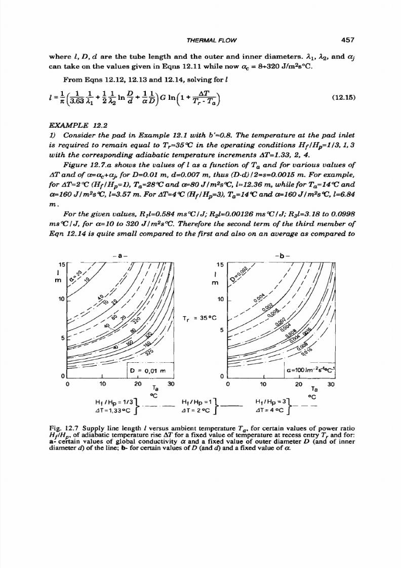
8/9/2019 Hydrostatic Lubrication 1992
http://slidepdf.com/reader/full/hydrostatic-lubrication-1992 474/558
THERMAL FLOW 457
where
1 ,
D , d are the tube length and the outer and inner diameters. A1, &, and Glj
can take on the values given in Eqns 12.11 while now cl, = 8+320 J/m2s°C.
From Eqns 12.12,12.13 and 12.14, solving for
1
(12.15)
EXAMPLE 12.2
1) Consider the pad in Example 12.1 with
b'=0.8.
The temperature at the pad inlet
is required to remain equal to Tr=350C in the operating conditions HflHp=1/3, ,3
with the corresponding adiabatic temperature increments AT=1.33, 2, 4.
Figure 12.7.a shows the values of 1 as
a
function of T,, and for various values of
AT and of a=cl,+aj or D=O.Ol m, d=0.007m, thus (D-d)l2=s=O.o015m. For example,
for
AT=2 c (Hf IHp=l ) ,Ta=280Canda=80JlmzsoC, ll12.36 m, while for Ta=l4oCand
e l 6 0 JlmzsoC, 1=3.57 m. For AT=4cY: HflHp=3),Ta=14cY:and -160 JlrnzsoC, 1=6.84
m .
For the given values, Rll=0.584 m s V lJ; R21=0.00126 m s v l J; R31=3.18 to
0.0998
ms@lJ, for a=10 to 320 Jlm2sV. Therefore the second term of the third member
of
Eqn 12.14 is quite small compared to the first and also on an average as compared to
- a -
15
1
m
10
5
0
10 20 30
Ta
0
-b -
1 5
I
m
10
T, = 35OC
5
0
0
10
20 30
Ta
OC
A T = 4 O C
f / H p = 3 1 -
--
Fig.
12.7
Supply line length I versus ambient temperature T,, for certain values of power ratio
H Hp .
of adiabatic temperature
rise
AT for a
f ixed
value
of
temperature at recess entry
T ,
and
for:
a-
certain values of global conductivity
a
and a fixed value
of
outer diameter D (and
of
inner
diameterd)of the line;
b-
for certain values of D andd)and a fixed value of a.
8/9/2019 Hydrostatic Lubrication 1992
http://slidepdf.com/reader/full/hydrostatic-lubrication-1992 475/558
458
HYDROSTATIC LUBRICATlON
the
third . Zt certainly becomes negligible for tube s wi th h igh t her m al con ductivity,
for exam ple, for copper tubes for w hich
&=300
J l m s V . There fore the in fluence o f d
is also often negligible an d the results presented are also valid fo r differ en t values
of
d , for lower values ( that
is
for higher values of thickness
s)
and even more
so
f o r
higher va lues (tha t is for lower values of
s).
Figure 12.7.6 shows the values of
1
as a function of T, and f or var ious values of
AT, D and d , for a=100 J I m 2 s T . The values of D and d are: D=0.002, 0.004, 0.008,
0.016
m;
d=O.001, 0.0025, 0.0055, 0.011 m ;
s=0.0005,0.00075,0.00125,
.0025 m ; th e
smaller values correspond to capillary tubes. For example, for AT=2 "c (HflH,,=l),
T=14"c and D=0.016 m, still 1=3.57 m, while for D=0.032 m and d=0.028 m (not plot -
te d) 1=3.11
m. As
regards d an d s th e above considerations still hol d good.
2) Pad w it h b'=0.95. Since AT and especially
Q
are lower t h a n the va lues relevant to
the pa d wi th b'10.8, length 1 is also lower.
For
example, for AT=1.85"C (HfIHp=l),
Tr=35"c , T ,=14"c0, for a d 6 0 JJm2s°C ,D=O.Ol m, d=0.007 m, the length is 1=1.72 m;
for -100 Jlm 2s "c , D= 0.016m , d=0.011 m, still 1=1.72 m ; fo r -100 Jl m 2s "C , D=0.032
m, d=0.028
m,
1=1.50 m.
12.4 COMPENSATING ELEMENTS
The heating of the lubricant occurs in the bearing and in the regulation devices
as well, that i s fixed ones such as capillaries and orifices and variable ones
such
as
flow control valves, etc. The rise in temperature is still given by Eqn
5.7,
putting
H+Hp=O and replacing p s with the pressure drop Apc in the regulator, tha t is
APC
ATc =-
P C
(12.16)
The tube length required t o keep the inlet temperature Tc a t a given value, is
then again given by Eqn
12.15,
replacing
AT
with
ATc
and
T ,
with
Tc.
EXAMPLE
12.3
1) Pad w ith b'=0.8 in examp le 12.1.
Z f
it is compensated by a capillary with p=0.5,
Ap,=1.73.106 N l m 2 , thu s ATc=l"c; in this case, fo r exam ple for Tc=35"c, Ta=14"C,
@lo0 J/m % "C , D=0.016 m, d=0.011 m, the length is 1=1.83 m.
2)
Pad with b'=0.95. In this case for 8=0.5, pc=1.6.106 Nlm2, thus ATC=0.924'C
and in the same conditions as
in
the previous example, the len gth is 1=0.879 m.
12.5 PUMP
The heating of the lubri'cant also occurs in the pump.
If
q
is its
efficiency, the
temperature rise
of
the lubricant may be put in the form

8/9/2019 Hydrostatic Lubrication 1992
http://slidepdf.com/reader/full/hydrostatic-lubrication-1992 476/558
1-71PiT
AT,= --
71 P C
THERMAL FLOW
459
(12.17)
where
pz=Apc+pr.
The tube length required t o keep temperature
T ,
entering the pump at a given
value, is then again given by Eqn 12.15, replacing
AT
with
AT,
and
T,
with
TT
EXAMPLE 12.4
1) Pad with b'=0.8
in
example 12.1. It
is
supplied by
a
pump
with an efficiency (for
example) q=0.8.
I f
the pad
is
supplied directly, p,=p,=1.73.106 N lmz and
ATZ=0.25 c; n this case, for T,=35 c, Ta=14 c,
-100
Jlm% c, D=0.016 m, d=O.011
m, the length is 1=0.464
m. I f
the pad is compensated, for p=0.5, p,=3.46.106 Nlm2,
AT,=0.5
"c
and 1=0.923 m.
2) Pad with b'=0.95. It is supplied by a pump with an efficiency q=0.8. If the pad
is
supplied directly, now p,=16,105 Nlm2 and AT,=0.231 C; n this case, in the same
conditions
as
in the previous example, the length is 1=0.223 m. I f the pad is compen-
sated, for p=O.S, p,=3.2.106 Nlm2, ATz=0.462 c and
1=0.444
m.
12.6 COOLING PIPELINES
Cooling can occur in the supply tubes between the pump and the bearing, as
already seen in section 12.3, as well as in the return tubes between the bearing and
the pump. If the bearing is directly supplied, and cooling occurs in the supply tube,
it s length is still given by Eqn 12.15,where
AT
is substituted by the total temperature
rise
ATT = AT, + AT
(12.18)
If cooling occurs in the return tube, 1 is still given by Eqn 12.15, where again
AT
is substituted by
ATT
in Eqn 12.18,and
T,
by
(T,-AT,).
Consequently I is
a
little larger
than in the previous case because the mean temperature
of
the lubricant in the tube
is a little lower.
If
the bearing is compensated and cooling occurs in the supply tube, 1 is still
given by Eqn
12.15,
where
AT
is substituted by the total temperature rise
ATT
=
ATz
-I-
ATc
-I-
AT
(12.19)
and
T,
by
(T,-AT,).
If
cooling occurs in the return tube, in Eqn
12.15
AT
is
substituted by
ATT
in Eqn
12.19, and
T,
by
(Tr-ATc-AT,).
8/9/2019 Hydrostatic Lubrication 1992
http://slidepdf.com/reader/full/hydrostatic-lubrication-1992 477/558
460 HYDROSTATIC LUBRICATION
In common practice, temperature
T ,
at the inlet of the pump
is
often taken as a
reference value. In this case, with compensation and cooling in the supply tube
where
T,=T,
referred to
T,
is
T ,
=
T, + AT.
If, on the other hand, cooling occurs in the return tube
(12.20)
(12.21)
where
T,
referred to
T,
is now
T,= T,
-
ATc
-
AT,
(12.22)
In the case of direct supply, the previous expression without
ATc
still holds good.
If the return tube
is
used as the cooler, larger diameters and small thicknesses
may be selected while on the contrary they must be avoided if cooling occurs in the
supply tube because tube elasticity could have a negative influence on the dynamic
stability of the bearing. If cooling occurs in the return tube, however, a recirculation
pump
is
almost always necessary. Therefore there
is
a further temperature rise
ATnp,
still expressed by Eqn
12.17,
but generally quite small since pressure head
ATnp,even with filters, is small.
Further temperature increments may occur in other elements of the circuit, in
particular in the filters, for which
ATp
can be calculated with Eqn
12.16,
ubstitut-
ing
Apc
with the pressure drop App in the filter, and also in the relief valve, for
which
AT,,is
again given by Eqn
12.16,
ut only for the lubricant escaping from
it.
In the case of compensation and cooling in the supply tube, in Eqn
12.20,AT,,
and ATq are added to
ATT
; f cooling occurs in the re turn tube, in Eqn
12.21 ATnp
is
added to
AT,
as well as
ATv
and
ATp
while i t must be subtracted in Eqn
12.22.
In the case of direct supply what has been said above still holds good but the
expressions lack the term
ATc.
EXAMPLE
12.5
Compensated supply with cooling in the supply tube.
1)
Pad with b'=0.8;
H f I H p = l ,
AT=2OC
(see
example
12.1).
For
8=0.5, dpC=1.73.1O6
N l m 2 a n d ATc=l
"c;
for App=0.3.106N lm 2 (roughly), ATp=0.173"c; he temperature
rise in the valve
i s
assumed (very roughly) to be AT,,=0.05°C. p ,=1.73.106 N l m z ,
8/9/2019 Hydrostatic Lubrication 1992
http://slidepdf.com/reader/full/hydrostatic-lubrication-1992 478/558
THERMAL FLOW
461
therefore, for q=0.8, ATn=0.544 c. The total temperature rise is then dT ~3 .7 7 C.
Putting Tr=35 c, Tn=370C.
For
Ta=14 c, e l 0 0 J/m2s0C,D=0.008 m, d=0.0055
m,
Eqn 12.20 yields 1=8.49 m.
2) Pad with b'=0.95;
H f I H p = l ,
AT=1.85 C. Ap,=1.6,106 Nlm2 and ATC=O.924 C,
AT,=0.173°C, ATv=0.050C;pr=16.106Nlm2 and ATn=0.505V; then A T ~ 3 . 5 c nd
Tn=36.850C.For the former values of T,, a, D and d, L=4.11 m. As seen above, the
length is almost unchanged even for lower values of d.
EXAMPLE 12.6
Cooling in the return tube
1) Pad with b'=0.8. Compared to the previous case
we
still have AT=BOC, AT,=l "C,
AT,=O.l 73 c, ATv=0.O5 C, but ATz=O.5OC and including the recirculation pump
with
q=O.8
and discharge pressure pnP=0.3.1O6N/m2, ATnp=0.0433
"C.
Then
AT~3.77 c nd Tp33.6V. For the former values of T,,
4
whereas D=0.032 m and
d=0.028 m, Eqn 12.21yields 1=6.06 m.
2) Pad with b'=0.95. Now ATn=0.4620C, thus A T ~ 3 . 5 c nd Tn=33.50C.For the
former values of the other quantities, 1=2.93m.
It must be noted tha t heat losses may occur in the bearing as well as in the other
elements of the circuit: in the pumps (for which efficiency losses also depend on
lubricant losses), in the compensator, especially in the capillary tubes, in the filters,
especially at high pressures, in the valves, etc. The lubricant may be cooled further
in the reservoir if this is reasonably sized (Appendix
2)
and finned (ref.
12.2).
More-
over
it
should also be noted that the set of supply tubes of a hydrostatic system can
work as the tube bank of an air-oil heat exchanger. Assuming that, on average,
50%
of the cooling ra te pertains t o all the other elements of the system, the length of the
cooling tube would be reduced by more than 50%' approximately.
12.7
SELF-COOLING CAPILLARY TUBE
Consider a capillary tube through which a pressure drop Ap, occurs. Its length
is easily determined from Eqn 4.66:
(12.23)
On
the other hand, the pressure drop produces heat, therefore there is a rise in
temperature AT, of the lubricant flowing through it, given by Eqn
12.16.
Heat, how-
ever, can be dissipated by a tube of the following length:
(12.24)
8/9/2019 Hydrostatic Lubrication 1992
http://slidepdf.com/reader/full/hydrostatic-lubrication-1992 479/558
462 HYDROSTATIC
LUBRlCA
T/ON
where Tc is the temperature a t the inlet of the tube. The tube may even be the capil-
lary itself. The diameters of the capillary must be related, in accordance with the
typical equation of thick pressurized tubes:
(12.25)
where p is the maximum nominal pressure in the tube, o he material limiting
stress and m the longitudinal deformation modulus. Actually, for construction
requirements, Eqn
12.25
is already satisfied for small diameter tubes.
Solving the system of three equations yields the dimensions of the self-cooling
capillary. As may also be seen in Fig. 12.8, it will be much longer than the length
given by Eqn 12.23 for very small values of d. Anyway, d must be large enough t o
avoid clogging (d>0.5.10-3m).
EXAMPLE 12.7
The capillary is made of drawn steel with the following characteristics:
0=3.5.107 Nlm2, so that elastic deformations are negligible, m=10/3.
1) Pad with b'=0.8 in example 12.1;B=0.5, thus Apc=1.73.106 N lm2 and ATc=l C.
The operating pressure is at a maximum at the inlet of the capillary tube and it is
p~= 3.4 6. 106 lmz ; for the maximum nominal pressure in Eqn 12.25 the value
assumed is p=4pM=13.9'106N l m2, also considering possible dynamic overloading;
Tc=35 c.
Figure 12.8.a shows length 1, capillary tube inner diameter d and outer diame-
ter D, as functions of ambient temperature T,, for a given value of overall conduc-
tance a=lOO Jlm2s C. It can be seen,
for
example, that for T,=lO C, 1=2.6 m,
d=0.0026 m and D=0.0042 m; while for Ta=2O C,1=4.1 m, d=0.0029 m and D=0.0047
m. In any case l l d is always much greater than 100, as usual for capillaries.
In
Fig. 12.8.b
1,
d and
D
are plotted as functions o f
a
for Ta=15V.It may be seen,
for example, that for a=60 Jlm% C, 1=4.2 m, d=0.0029 m and D=0.0047 m; while for
a=120 J/mZs C, 1=2.9 m, d=0.0027 m and D=0.0043 m. Capillaries may be wound i n
large pitch spirals.
2) Pad with b'=0.95;
/3=0.5,
hus Apc=1.6.106 N l m z and ATc=0.9240C; p=12.8.106
Nlm2 is assumed; TC=35 c. n Fig. 12.8 1, d, and D are plotted as functions of Ta a)
as functions of a (b). Length and diameters are smaller than those in the previous
case.
The results obtained apply even more
t o
copper capillary tubes; however,
it
is
advisable to increase the outer diameter by 25% with no detriment to cooling which

8/9/2019 Hydrostatic Lubrication 1992
http://slidepdf.com/reader/full/hydrostatic-lubrication-1992 480/558
THERMAL
FLOW
463
- a -
- b -
~~
-
T = 350C , T = I 5 OC
b‘ =
0.8 ___
- - - _ _
- -
_
- - _
-
-
0.0075
D,
d
m
0.005
3.0025
3
0
10
20 30 0 40 80 120 a 160
Ta
OC
J m-*s-’
o c - 1
Fig.
12.8
Length
I,
outer diameter
D
and inner diameter
d
of a self-cooling capillary tube
of
a
bear-
ing with a recess width b‘,versus: a- ambient temperature T,, for a fixed value of temperature enter-
ing tube
T,,
and global conductivity a; b- a, for fixed va lues of T , and T,.
is still higher than in steel capillaries because of the much higher conductivity of
copper as compared to steel.
In general, the design
of
a self-cooling capillary, without solving the system of
three equations, may be carried out as follows:
assign
d
(for instance, with the aid of Fig. 12.8);
from Eqn 12.23 determine
I
and introduce it into Eqn 12.24 without the generally
negligible term (1/2)(1/&)ln(D/d); thus determine D;
22D/d21.5 should be satisfied, instead of Eqn 12.25, otherwise:
the procedure is repeated until the result is achieved.
12.8
VISCOSITY
AND
TEMPERATURE
Up to now viscosity has been assumed to be constant as temperature varies,
especially in the pad film. This can be considered to be true if heat dissipation in the
various elements of the hydrostatic system keeps the increment in the lubricant
temperature low, especially if the supply and return tubes and the reservoir are
designed as coolers. Otherwise the new value of viscosity in the film must be evalu-
ated according
to
the mean value of temperature, and calculations must be repeated
until the difference between two consecutive values of viscosity is sufficiently small.
In the case of compensated supply the actual value of viscosity in the compensating
8/9/2019 Hydrostatic Lubrication 1992
http://slidepdf.com/reader/full/hydrostatic-lubrication-1992 481/558
464
HYDROSTATIC LUBRICATION
elements must be taken into account. When lubricant temperature is under control,
the hydrostatic system operates properly and thermal deformations of the bearings,
detrimental
t o
the smooth running of the machine and the accuracy of products in
the case of
a
machine tool, are avoided.
REFERENCES
12.1
Bird
R.
B., Stewart
W. E.,
Lightfoot E.
N.;
Transport Phenomena;
Wiley and
12.2
Kreith
F.;
Principles of Heat Transfer;
Intext Educational Publisher,
N.Y.,
Sons,1960; 780 pp.
1973;
50 pp.
8/9/2019 Hydrostatic Lubrication 1992
http://slidepdf.com/reader/full/hydrostatic-lubrication-1992 482/558
Chapter 13
EXPERIMENTAL TESTS
13.1 INTRODUCTION
An important aspect of the study of hydrostatic bearings
is
testing them, con-
sisting in the measurement of a considerable number of input and output variables
of the hydrostatic system. This, together with the large number of types of bearings,
has led to the assembly of a considerable number of test rigs, only a few of which are
equipped for the testing of more than one type of bearing.
In this chapter, af ter some brief notes on the most important input and output
variables and testing procedures, a number of test rigs are described, chosen
among
a
host of equally good rigs, and details are given of the tests performed on a
few particular types of bearing.
13.2 HYDROSTA TIC SYSTEMS; INPUT AND OUTPUT VARIA BL ES
There a re many variables affecting a tribological system and a hydrostatic sys-
tem in particular, as shown in Fig.
13.1.
The behaviour of the mechanical system
made up
of
a pad and a slide separated by lubricant and placed in the atmosphere,
depends on numerous input variables and it is also characterized by the output
variables; the validity of the tests largely depends on the correct experimental
measurement of such variables. The following input variables are examined:
the type of motion, which is sliding in hydrostatic lubrication;
speed, which can be linear
o r
angular and the control and measurement of which
is
carried out with electronic tachometers, which are especially necessary for very
low or very high speeds;
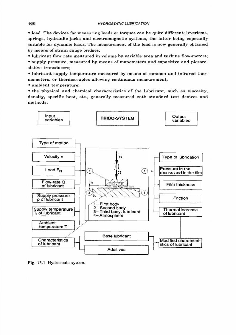
8/9/2019 Hydrostatic Lubrication 1992
http://slidepdf.com/reader/full/hydrostatic-lubrication-1992 483/558
466 HYDROSTATIC LUBRICA TlON
load. The devices
for
measuring loads or torques can be quite different: leverisms,
springs, hydraulic jacks and electromagnetic systems, the la tter being especially
suitable for dynamic loads. The measurement of the load is now generally obtained
by means
of
strain gauge bridges;
lubricant flow rate measured in volume by variable area and turbine flow-meters;
supply pressure, measured by means
of
manometers and capacitive and piezore-
sistive transducers;
lubricant supply temperature measured by means of common and infrared ther-
mometers, o r thermocouples allowing continuous measurement;
ambient temperature;
the physical and chemical characteristics
of
the lubricant, such as viscosity,
density, specific heat, etc., generally measured with standard test devices and
methods.
Input
variables
Typeof motion
m
elocity v
I
LoadFN
I r t
Supply pressure
D
of
lubricant
T
RIB -SYST EM
utput
variables
1-
First body
2- Second body
3-
Third body: lubricant
i
- Atmosphere
4
ype of lubrication
I
I 1
f T i G m - l
recess and in the
film
{Filmthickness)
1
Friction
Thermal increase
of lubricant
L
Base lubricant I
Modified charatcteri-
haracteristics
of lubricant stics of lubricant
Additives
Fig. 13.1
Hydrostatic system.
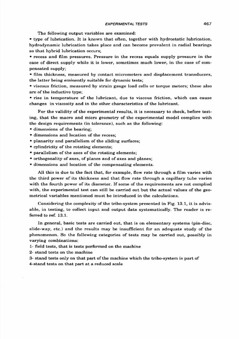
8/9/2019 Hydrostatic Lubrication 1992
http://slidepdf.com/reader/full/hydrostatic-lubrication-1992 484/558
EXPERIMENTAL TESTS 467
The following output variables are examined:
type of lubrication. It
is
known that often, together with hydrostatic lubrication,
hydrodynamic lubrication takes place and can become prevalent in radial bearings
so
that hybrid lubrication occurs;
recess and film pressures. Pressure in the recess equals supply pressure in the
case of direct supply while it is lower, sometimes much lower, in the case of com-
pensated supply;
film thickness, measured by contact micrometers and displacement transducers,
the latter being eminently suitable
for
dynamic
tests;
viscous friction, measured by strain gauge load cells or torque meters; these also
are of the inductive type;
rise in temperature
of
the lubricant, due to viscous friction, which can cause
changes in viscosity and in the other characteristics of the lubricant.
For the validity of the experimental results, it is necessary to check, before test-
ing, that the macro and micro geometry of the experimental model complies with
the design requirements (in tolerance), such as the following:
dimensions of the bearing;
dimensions and location of the recess;
planarity and parallelism
of
the sliding surfaces;
cylindricity of the rotating elements;
parallelism of the axes of the rotating elements;
orthogonality of axes, of planes and of axes and planes;
dimensions and location
of
the compensating elements.
All this is due to the fact that, for example, flow rate through a film varies with
the third power
of
its thickness and that flow rate through a capillary tube varies
with the fourth power of its diameter.
If
some of the requirements are not complied
with, the experimental test can still be carried out but the actual values of the geo-
metrical variables mentioned must be introduced in the calculations.
Considering the complexity of the tribo-system presented in Fig.
13.1,
it
is
advis-
able, in testing, t o collect input and output data systematically. The reader is re-
ferred to ref. 13.1.
In general, basic tests are carried out, that is on elementary systems (pin-disc,
slide-way, etc.) and the results may be insufficient for an adequate study of the
phenomenon.
S o
the following categories of tests may be carried out, possibly in
varying combinations:
1-field tests, tha t is tests performed on the machine
2-
stand tests
on
the machine
3-
stand tests only on that part of the machine which the tribo-system is part of
4-stand tests on that par t a t a reduced scale

8/9/2019 Hydrostatic Lubrication 1992
http://slidepdf.com/reader/full/hydrostatic-lubrication-1992 485/558
468
HYDROSTATIC LUBRICATION
POTENTIOMETER
4
5-tests on the tribo-system taken off the part of machine containing
it
6-basic tests, already mentioned.
- V D C + DETECTOR
-A
0
10
1 0
30--100
r.
,
13.3
EXPERIMENTAL
RIGS
13.3.1 Electr ic analog f ie ld p lot ter
The apparatus shown in Fig. 13.2.a is not an experimental bearing but a device
for the determination of the characteristics of the bearing through the use of an
electric analog field plotter which w a s being used some decades ago in the study of
hydrostatic bearings of various shapes, giving satisfactory results. It is based on the
fact that Reynolds equation, which allows us to calculate pressure distribution in
the bearing clearance, is analogous to the electric field equation which makes it
possible t o calculate voltage distribution in a conducting sheet with the shape of the
clearance. Figure 13.2.a contains an outline of the circuit of the electric analog field
plotter (ref. 5.34).
- a -
- b -
E l
SILVER
.
ECT
RODES-
11OV ]16VAC
I
AC
8
7
6
5
4
3
2
1
0
a
80
70
60
50
40 0
30
20
10
0
n
I
0 0.2 0.4
0.6 0.8
1.0
'1
1'2
Fig.
13.2 Electric analogy: a- Circuit of the electric field plotter; b- Performance factors of a cir-
cular thrust
bearing
Figure 13.2.b gives the values of the pressure in the recess, of the flow rate and
the pumping power as functions
'of
the radius,
as
obtained with the plotter
for
a
circular bearing (ref. 13.2). As can be seen, there is a remarkable agreement be-
tween these and the theoretical results (solid lines).

8/9/2019 Hydrostatic Lubrication 1992
http://slidepdf.com/reader/full/hydrostatic-lubrication-1992 486/558
EXPERIMENTAL
TESTS
469
13.3.2
Axial bearings
i)
Device simulating
a
hydrostatic p a d .
Of the numerous types of experimental
thrust bearings, a circular and particularly simple one (ref. 13.3), shown in Fig.
13.3, is examined. Pad 1, axially free to move in seat 2 , is subjected t o a load pro-
duced by spring 3. The load can be varied by varying the spring tension by means of
screw 4. The load is balanced by the pressure in the recess and in the film, the
thickness of which is measured with micrometer
5 .
The friction between pad
1
and
seat 2 is lowered by the lubricant between them. Though lacking precision mainly
because of friction, the device is quite useful for investigating circular pads with
ratio
r21r2
equal t o the experimental one.
Fig. 13.3
Device simulating a hydrostaticpad.
With devices similar to that in Fig. 13.3, though less precise, differently shaped
pads (rectangular, etc.) can be tested. If pads are supported radially by aerostatic
bearings, there i s almost no friction, thus the results are more precise.
ii) Turn-tab le simulat ing a sl iding table . Figure 13.4.a shows a (tilted) circular
pad tested (ref. 13.4) with the apparatus outlined in Fig. 13.4.b. The test rig consists
of a turn-table substituting a sliding table; this does not imply there are large errors
because the turn-table
is
much larger (about 1.2 m) than the test pad (about 0.1 m)
placed at its periphery. The turn-table is supported and located by three pairs of
opposed hydrostatic thrust pads equally spaced out around the structure. The test
pad is attached to the base of a plunger which is located in a cylinder rigidly
mounted on the base of the test rig. Free vertical movement of the plunger is as-
sured by two rows of air bearings in the wall of the cylinder. Loads are applied t o the
test pad by adding weights
to
the plunger, and the tilt of the test pad with respect to
the table is introduced by shims.
In Fig. 13.4.c the variation of the dimensionless flow rate
Q=Qp/@oh$
s
plotted
as a function of the "dynamic term"
S=6pRz(Ua+2V) l (pohg) ,
where U and V are the
sliding and the squeeze velocities, respectively, for certain values of the angle of ti lt
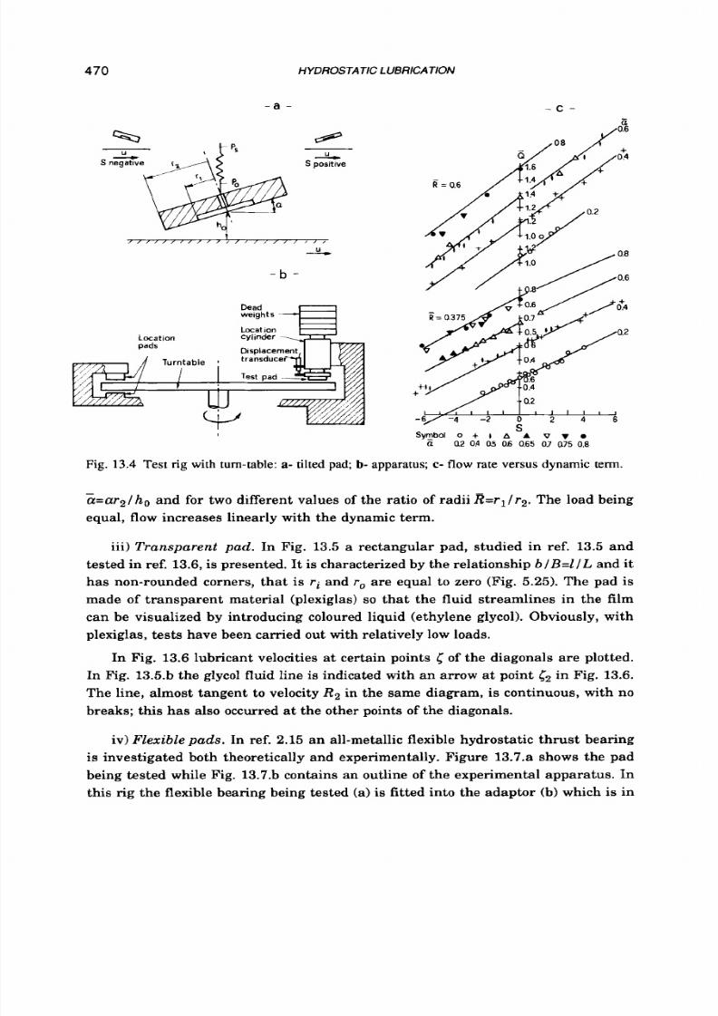
8/9/2019 Hydrostatic Lubrication 1992
http://slidepdf.com/reader/full/hydrostatic-lubrication-1992 487/558
470
HYDROSTATIC LUB RICATION
- a - - c -
S
positive
u
- b -
u
SyEbol
0
+ I A A v v
a a2 04 a5
OB
065 07 a75 0.8
Fig. 13.4 Test
r i g with
turn-table: a- tilted pad;
b-
apparatus; c- flow rate versus dynamic term.
-
a=ar2/ho nd for two different values
of
the ratio of radii iZ=rl/r2.The load being
equal, flow increases linearly with the dynamic term.
iii)
Transparen t pad .
In Fig. 13.5 a rectangular pad, studied in ref. 13.5 and
tested in ref. 13.6, is presented. I t is characterized by the relationship
b I B = l I L
and it
has non-rounded corners, that is ri and
r,,
are equal t o zero (Fig. 5.25). The pad is
made of transparent material (Plexiglas)
so
that the fluid streamlines in the film
can be visualized by introducing coloured liquid (ethylene glycol). Obviously, with
Plexiglas, tests have been carried out with relatively low loads.
In Fig. 13.6 lubricant velocities at certain points [
f
the diagonals are plotted.
In Fig. 13.5.b the glycol fluid line is indicated with an arrow a t point
c2
in Fig. 13.6.
The line, almost tangent to velocity
Rz in
the same diagram, is continuous, with no
breaks; this has a l s o occurred a t the other points of the diagonals.
iv)
Flexible p a ds .
In ref. 2.15 an all-metallic flexible hydrostatic thrust bearing
is investigated both theoretically and experimentally. Figure 13.7.a shows the pad
being tested while Fig. 13.7.b contains an outline of the experimental apparatus. In
this rig the flexible bearing being tested (a)
is
fitted into the adaptor (b) which is in
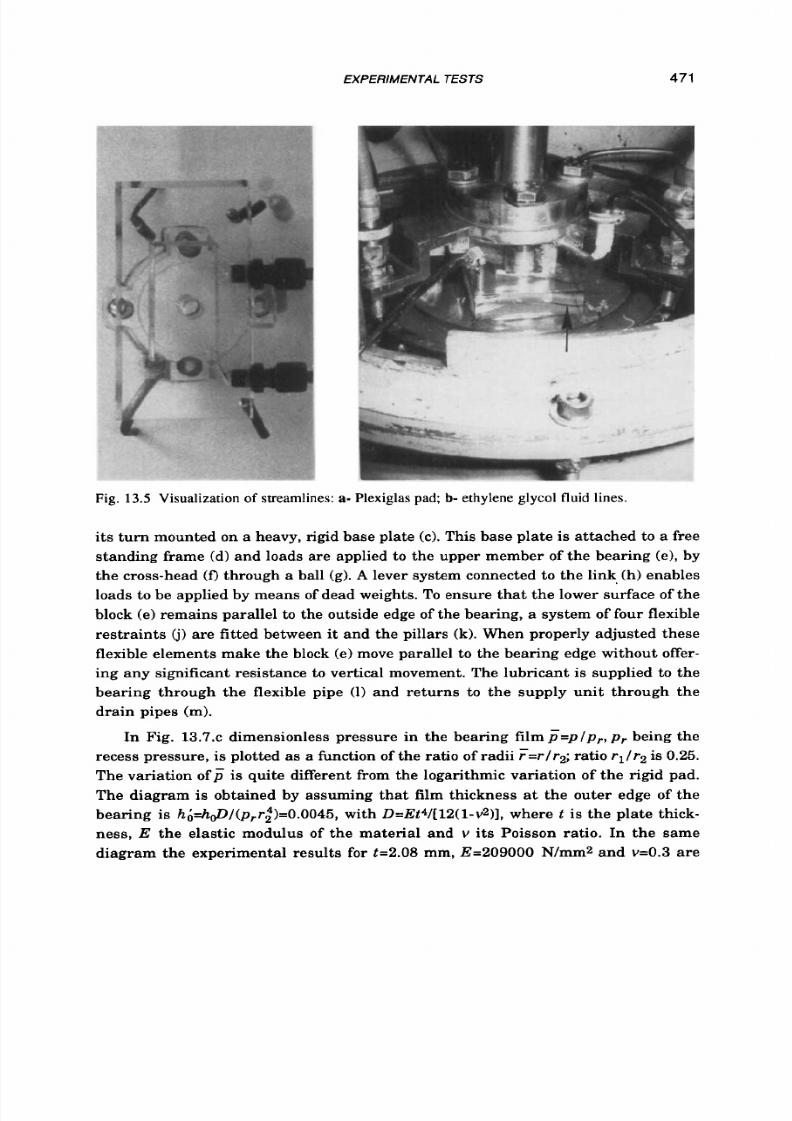
8/9/2019 Hydrostatic Lubrication 1992
http://slidepdf.com/reader/full/hydrostatic-lubrication-1992 488/558
EXPERIMENTAL
TESTS
471
Fig.
13.5
Visualization
of
streamlines:
a-
Plexiglas pad;
b-
ethylene glycol fluid lines.
its turn mounted on a heavy, rigid base plate (c). This base plate is attached
t o
a free
standing frame (d) and loads are applied t o the upper member of the bearing (e), by
the cross-head
(f)
through a ball (g). A lever system connected t o the link. (h) enables
loads to be applied by means of dead weights. To ensure that the lower surface of the
block (e) remains parallel to the outside edge of the bearing, a system of four flexible
restraints c) are fitted between it and the pillars (k). When properly adjusted these
flexible elements make the block (e) move parallel to the bearing edge without offer-
ing any significant resistance
t o
vertical movement. The lubricant is supplied to the
bearing through the flexible pipe (1) and returns to the supply unit through the
drain pipes (m).
In Fig. 13.7.c dimensionless pressure in the bearing film F=p/pr,pr being the
recess pressure, is plotted as a function of the ratio of radii r= r/r2;ratio r1/r2 is 0.25.
The variation of is quite different from the logarithmic variation of the rigid pad.
The diagram is obtained by assuming that film thickness a t the outer edge of the
bearing is h&h&/(p,r$)=0.0045, with D=Et4/[12(1-v2)],where t is the plate thick-
ness,
E
the elastic modulus
of
the material and
v
its Poisson ratio. In the same
diagram the experimental results for t =2 . 08 mm, E=209000 N/mm2 and v=0.3 are

8/9/2019 Hydrostatic Lubrication 1992
http://slidepdf.com/reader/full/hydrostatic-lubrication-1992 489/558
472
HYDROSTATIC LUBRICATION
Fig. 13.6 Velocity of
fluid at
certain points of a diagonal.
also given.
It
should be noted that the effectiveness of flexible bearings decreases as
the recess increases.
13.3.3
Radial bear ings
i) Test rig
for
static loads. In Fig. 13.8 a test rig for radial bearings subjected to
static loads (ref. 10.9) is shown. A shaft driven by a variable-speed motor, is sup-
ported a t both ends by roller bearings and a block of the hydrostatic bearing floating
on the middle of the shaft. In both sides of the floating block there are hydrostatic
thrust bearings. A static load is applied by pulling up the floating block, using a
ring.
With such an apparatus it is possible
to
investigate the occurrence, in the pres-
ence of static loads, of forced vibrations caused by the fluctuations in recess pres-
sure due to aeration of the working fluid, as well as self-excited vibrations of larger
amplitudes, i.e. oil-whirl. The appearance of recess pressure P,. lower than ambient
pressure is considered as the boundary of the allowable operating range. This
boundary, for the upper pad of a four-pad capillary compensated bearing, is given in
Fig. 13.9, as a function of the eccentricity ratio
E=elho
and of the speed parameter or
Sommerfeld hybrid number S = p o fP J c fD)2 (where c is the diametral clearance and
D s the journal diameter), for certain values of load
F.
ii)
Experimental apparatus
for
static and dynamic loads.
Figure 13.10.a shows a
test rig for journal bearings subjected
t o
both static and dynamic loads (ref. 13.7).A s

8/9/2019 Hydrostatic Lubrication 1992
http://slidepdf.com/reader/full/hydrostatic-lubrication-1992 490/558
EXPERIMENTAL TESTS
473
- a -
- c -
I 4 1
0.3
04
0.5 06 0.7 0.8 0.9 1.0
Dimens ion les s r a d i u s ,
T
Fig. 13.7 Flexible hydrostatic thrust bearing:
a-
pad;
b-
experimental apparatus;
c-
pressure
versus radius.
in the previous case, a shaft
(A)
driven by a motor
(B)
through a n elastic joint (C) is
supported by two roller bearings mounted in a trunnion assembly
(D)
nd the block
(El
of the hydrostatic bearing is floating on the middle of the shaft. Eight symmetri-
cally-placed flexible restraints (F)ensure that the bearing bIock moves perpendicu-
larly t o the shaft without imposing any significant restraint. Steady loads are ap-
plied to the bearing by the screwjack ( G ) hrough the calibrated spring (H). Oscilla-
tory loads are applied to the bearing by the electromagnetic vibrator
(I)
which is
mounted in a space provided in the base (L) mounted on four flexible supports
(M).
A strain gauge force transducer (N) easures the dynamic loads applied to the
bearing. '
The dynamic tests have been carried out on
a
four-recess orifice-compensated
bearing both with static loads and without them. Figure 13.10.b concerns the first
type of tests performed with the bearing at rest and shows the flexibility, or recep-
tance, f u as a function of the forcing frequencyaf=Qf/SZ of a sinusoidal load
(f2
being
the undamped frequency of the bearing) for an equal amplitude of oscillation
6,
around the centre, for two v a l ~ es f the supply pressure and with the pressure ratio
p=0.5. There is a good correspondence between the experimental and theoretical

8/9/2019 Hydrostatic Lubrication 1992
http://slidepdf.com/reader/full/hydrostatic-lubrication-1992 491/558
474
HYDROSTATIC
1
BRlCA
TlON
t
t r ans duc ers
J o u n a l b e a r i n g '
~~~~~~~~~~~~
b l o c k
Fig.
13.8
Experimental apparatus for journal bearings.
1.0
&
0 50 100 150
s
Fig.
13.9
Effeg of eccentricity ratio and speed parameter on the appearance of recess pressure
(dimensionlessP,=P,JP, where P, is supply pressure) lower than ambient pressure.
results up to +0.65, above which they differ because cavitation takes place in the
recess.
iii) Experimental apparatus for static and dynamic magnetic loads. The test rig
(ref. 13.8) shown in Fig. 13.11.a consists of a symmetrical rotor with a flywheel (1)
equipped with transformer steel sheets. Compressed air from a blower drives a
light turbine wheel (2). Symmetrically, there is an equivalent disc
(3)
for triggering
and sampling the signals measured. The rotor is supported by two identical hydro-
static bearings (4). The shaft is axially positioned by two
air
bearings (5 ) . External
vertical radial forces are applied by magnetic shoes
(6).
In order to induce basic
harmonic sinusoidal forces alone, a static component must be superimposed on the
top magnetic shoe. In this way the rotor is lifted up t o the concentric position in the
bearings. A bottom magnetic shoe is used to apply higher static load downwards.

8/9/2019 Hydrostatic Lubrication 1992
http://slidepdf.com/reader/full/hydrostatic-lubrication-1992 492/558
EXPERIMENTAL
TESTS
475
With this magnetic force system it is possible
to
vary the force frequency indepen-
dently of shaft rotation frequency. An appropriate set
of
instruments, such as
dynamometer (7) and eddy current probes (8),makes it possible to measure the vari-
ous variables.
- a -
C
B
N
- b -
supply pressure. lb / in2
o
0
0 66
n .
0
1 2
Dim ens ion les s f o r c ing t r equenc y , a
'
0 4 '
0 8
Fig. 13.10 Experiments on journal bearings:
a-
Experimental apparatus;
b-
Bearing response
curve.
- a -
- b -
Fig.
13.1
1
Experiments on journal bearings:
a-
Experimental apparatus;
b-
orbit
of
the shaft
centre.

8/9/2019 Hydrostatic Lubrication 1992
http://slidepdf.com/reader/full/hydrostatic-lubrication-1992 493/558
476 HYDROSTATIC LUBRICATION
Because of the hydrodynamic component, which is almost always also present
in hydrostatic bearings, a bearing subjected
to
both static and dynamic loads moves
on an orbit (characteristic of hydrodynamic bearings) around the static equilibrium
position. This is clearly shown by both the theoretical (solid line) and the experimen-
tal (dashed line) results contained in Fig. 13.11.b for a compensated four-recess-
bearing with 8=0.5, subjected t o
a
static load and t o a sinusoidal dynamic load
giv-
ing rise
t o
elliptical orbits. There is good agreement between the theoretical and the
experimental results. In the diagram E is the static eccentricity, S = p n / p , ( c
/
0 2 ) the
speed parameter, n the angular velocity and
fF
the dynamic load frequency.
13.3.4
Spher ica l bear ings
Figure 13.12. shows an experimental apparatus (ref. 5.25) for spherical bear-
ings (either the fitted or the clearance type). Pad (11, rigidly connected t o the rotating
shaft (2), is supported by the central recess bed (31, which is placed on the bed car-
rier (4). The bed carrier and the base (5) are adjusted by screws. The apparatus is
equipped with a set
of
instruments for the measurement of some of the variables
involved, in particular with mercury-in-glass manometers for the measurement of
pressure in the recess and in the film.

8/9/2019 Hydrostatic Lubrication 1992
http://slidepdf.com/reader/full/hydrostatic-lubrication-1992 494/558
EXPERIMENTAL TESTS 477
-b-
Fig.
13.13
Experiments
on
spherical bearings:
a-
outline
of
the bearing;
b-
Comparison between
experimentaland theoretical pressure distribution.
Fig. 13.14 Test-rig
for
screws and nuts,
In Fig. 13.13.b the theoretical pressures in a directly supplied bearing are plot-
ted, according to the isothermal assumption (solid line; the temperature
of
the fluid
remains constant because of heat transfer to the surrounding environment) and
according to the adiabatic assumption (dash-dot line; no heat transfer); PI s the
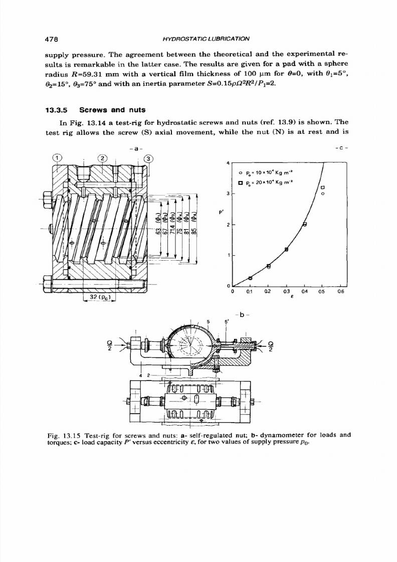
8/9/2019 Hydrostatic Lubrication 1992
http://slidepdf.com/reader/full/hydrostatic-lubrication-1992 495/558
478
HYDROSTATIC LUBRICATION
supply pressure. The agreement between the theoretical and the experimental re-
sults is remarkable in the latter case. The results are ghen for a pad with a sphere
radius R=59.31 mm with a vertical film thickness of 100 pm
for
8=0,
with
81=5",
(&=15O,
3=750
nd with an inertia parameter S=0.15pR2R2/Pl=2.
13.3.5
Screws and nuts
In Fig. 13.14 a test-rig
for
hydrostatic screws and nuts (ref. 13.9) is shown. The
test rig allows the screw (S) axial movement, while the nut
(N)
is at rest and is
- a -
; @
-b -
5'
- c -
4
o
p o = l O x l O ' ~ g r n ~ '
po=20110'Kg
m- '
3 -
P'
2 -
o 0.1 a2
03
04 05 06
&
Fig. 13.15 Test-rig for screws and nuts: a- self-regulated nut;
b-
dynamometer for loads and
torques; c- load capacity P' versus eccentricity E, for two values
of
supply pressurepo.

8/9/2019 Hydrostatic Lubrication 1992
http://slidepdf.com/reader/full/hydrostatic-lubrication-1992 496/558
EXPERIMENTAL TESTS
479
engaged in the dynamometer
(5)
which hides
it.
The base (2) carries the support (41,
then the dynamometer and then the nut; it also carries the four capillary compen-
sated bearings (3), which support the nut.
A
variable speed motor
(6)
moves the
screw, which
is
loaded axially by the hydraulic jack
(12).
The various joints elimi-
nate the effects of construction and assembly errors and those resulting from
strains in the structure under loads. The screw and nut being tested are self-
regulated. Figure 13.15.a shows the nut
(2)
with its two lateral seals (1) and (3)
which cannot entirely prevent leakages. The nut is supplied through the
dynamometer (Fig. 13.15.b) by means of two lateral pipes (5')of small diameter and
thickness equipped with strain gauges. So these pipes are supply lines and also part
of the dynamometer.
In Fig. 13.15.c the screw and nut load capacity
P'
is plotted as a function
of
ec-
centricity E , with the screw
at
rest. For
&=0.5
(and for higher values not shown in the
diagram but very frequent in common practice) the experimental values are re-
Fig.
13.16
Test-rig for slide-way: ( 1 ) slide-way,
(2)
frame, ( 3 ) hydraulic jack.
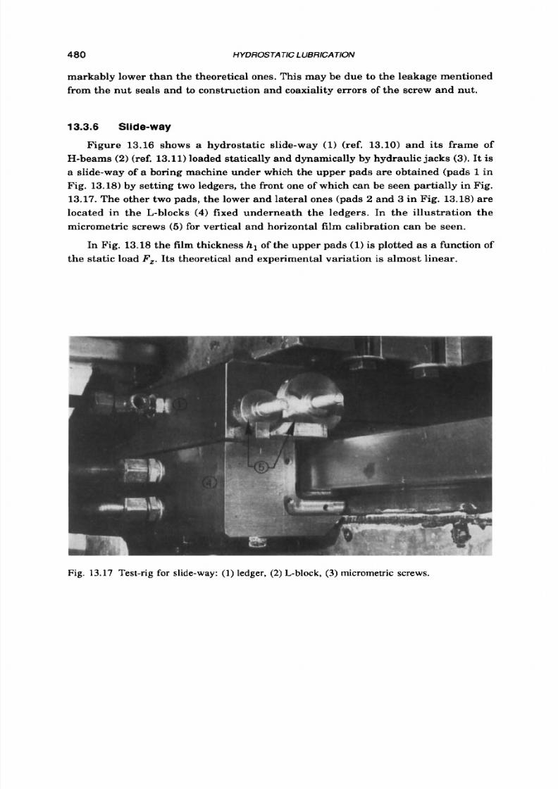
8/9/2019 Hydrostatic Lubrication 1992
http://slidepdf.com/reader/full/hydrostatic-lubrication-1992 497/558
480 HYDROSTATIC LUBRICAJlON
markably lower than the theoretical ones. This may be due to the leakage mentioned
from the nut seals and to construction and coaxiality errors of the screw and nut.
13.3.6
Slide-way
Figure
13.16
shows a hydrostatic slide-way
(1)
(ref.
13.10)
and
its
frame of
H-beams (2) (ref.
13.11)
loaded statically and dynamically by hydraulic jacks
(3).
It is
a slide-way of a boring machine under which the upper pads are obtained (pads
1
in
Fig.
13.18)
by setting two ledgers, the front one of which can be seen partially in Fig.
13.17.The other two pads, the lower and lateral ones (pads
2
and 3 in Fig. 13.18)are
located in the L-blocks (4) fixed underneath the ledgers. In the illustration the
micrometric screws
(5)
or vertical and horizontal film calibration can be seen.
In Fig.
13.18
the film thickness hl of the upper pads
(1)
is plotted as a function of
the static load
Fz.
ts theoretical and experimental variation is almost linear.
Fig. 13.17 Test-rig for slide-way: ( 1 ) ledger, (2) L-block, (3) micrometric screw s.
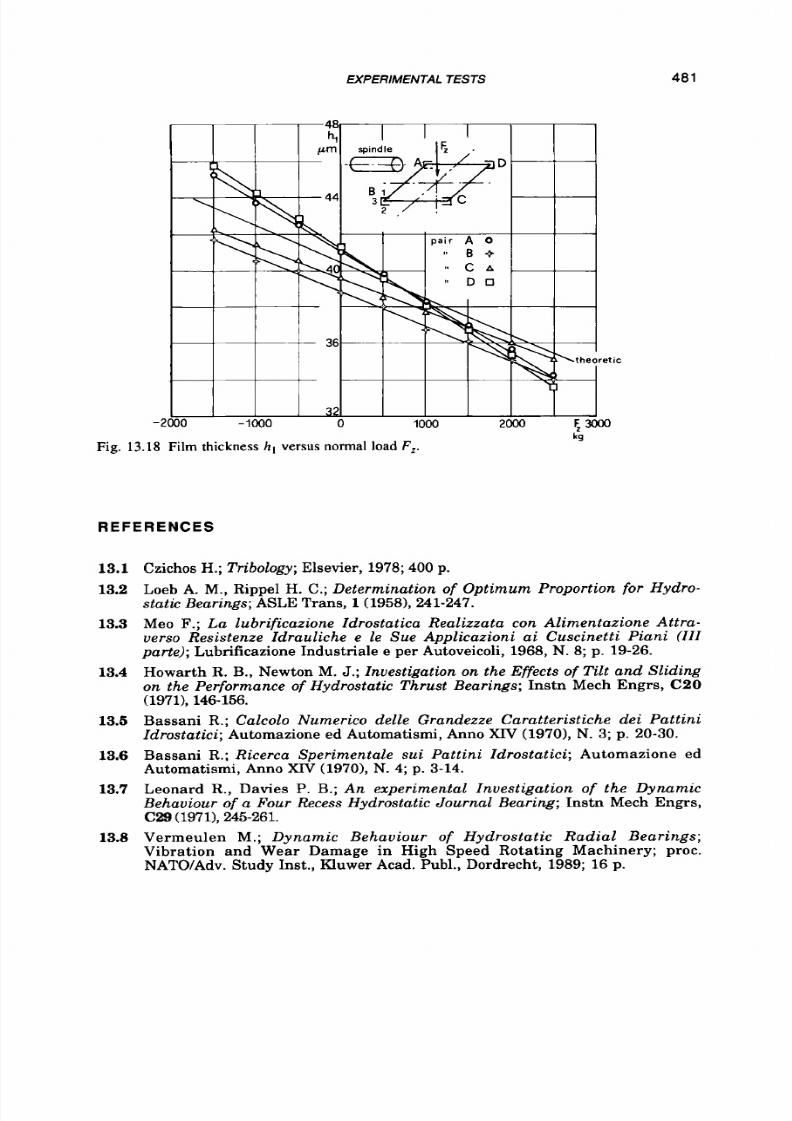
8/9/2019 Hydrostatic Lubrication 1992
http://slidepdf.com/reader/full/hydrostatic-lubrication-1992 498/558
EXPERIMENTAL TESTS
481
kg
Fig. 13.18 Film thickness h , versus normal load Fz .
R E F E R E N C E S
13.1
13.2
13.3
13.4
13.6
13.6
13.7
13.8
Czichos H.; Tribology;Elsevie r, 1978; 400 p.
Loeb A. M., Rippel
H.
C.; Determination of O pt im um Proport ion for Hydro-
static Bearings;
ASLE Trans,
1 (1958),
241-247.
Meo F.; La lubri f icazione Zdrostat ica Realizzata con Alimentazione Attra-
verso Resistenze Zdrauliche e le Sue Applicazioni ai Cuscinetti Piani (ZZZ
parte); Lubrificazione Industriale e per Autoveicoli, 1968,N.
8;
p. 19-26.
H o w a r t h
R.
B., Newton
M.
J.;
Invest igat ion on the Effects of Ti l t a nd Sl tding
on the Performance of Hydrostatic Thrust Bearings; Ins tn Mech Engrs , C20
Bassan i
R.; Calcolo Numeric0 del le Grandezze Caratterist iche dei Patt in i
Zdrostatici; Automazione ed Autom atismi, Anno XIV (1970),
N.
3; p. 20-30.
Bassan i R.; Ricerca Sperimentale sui Pattini Zdrostatici; Automazione ed
Autom atismi, Anno XIV (1970), N. 4; . 3-14.
Leonard R., Davies
P.
B.;
An
experimental Invest igat ion of the Dynamic
Behav iour o f a Four Recess Hydrostatic Journal Bearing ;
Ins tn Mech E ngrs ,
V e r m e u l e n M . ;
Dynamic Behav iour o f Hydros ta t i c Rad ia l Bear ings ;
Vibra t ion and Wear Damage in H igh Speed Rota t ing Mach inery ; p roc .
NATO/Adv. Stu dy In st. , Kluwer Acad. Publ., D ordrech t, 1989; 16 p.
(1971), 146-156.
C29
19711,245-261.

8/9/2019 Hydrostatic Lubrication 1992
http://slidepdf.com/reader/full/hydrostatic-lubrication-1992 499/558
482
HYDROSTATIC 1 BRlCATlON
13.9 Bassani
R.;
he Self-Regulated Hydrostatic Screw and Nut;
Tribology
Inter-
national, 12
(19791, 185-190.
13.10 Bassani
R.,
Culla C.; Progetto e Costruzione
di
una Slit ta di Macchina Uten-
sile, a Lubrificazione Zdrostatica; Atti 1st. Mecc.
Appl.
Costr. Macch., Univ.
di Pisa, Anno Acc. 1973-74,
N .
47; 69
pp.
13.11 Bassani R.,Culla C.; Progetto e Costruzione d i una Attrezzatura pe r Prove di
Carico su una Slit ta Idrostatica di Macchina Utensile . Primi Risultati Spe-
r imental i ; Atti 1st. Meccanica, Univ. di Pisa, AIM
7612,
1976;51
p.

8/9/2019 Hydrostatic Lubrication 1992
http://slidepdf.com/reader/full/hydrostatic-lubrication-1992 500/558
Chapter 14
APPLICATIONS
14.1 INTRODUCTION
In the first chapter we have already mentioned that hydrostatic lubrication has
been successfully applied in many branches of mechanical engineering, from
large, slowly rotating machines to small and fast machines.
In this chapter, a number of applications will be briefly described, beginning
with the very important field of machine tools. Certain types of hydrostatic tilting
pads used to build bearings for large machinery, such as telescopes, air preheaters,
ore mills, debarking drums, and so on will then be examined.
Lastly, after having mentioned a few applications of a different kind, a number
of supply systems will be described, with particular reference to constant-flow sys-
tems making use of flow dividers or multiple pumps.
14.2 MACHINE TOOLS
14.2.1 Spindles
Machine tool spindles form one of the most common fields of application of ex-
ternally pressurized lubrication, since a high degree of stiffness and damping (i.e.
precision characteristics) is required.
Hydrostatic spindles may be supported by separate journal and thrust bearings,
as well as by a couple of opposed conical bearings; in certain cases other configura-
tions may prove to be suitable: for instance, conical bearings may be substituted by
spherical bearings,
o r
an opposed-pad bearing and a journal bearing may be com-
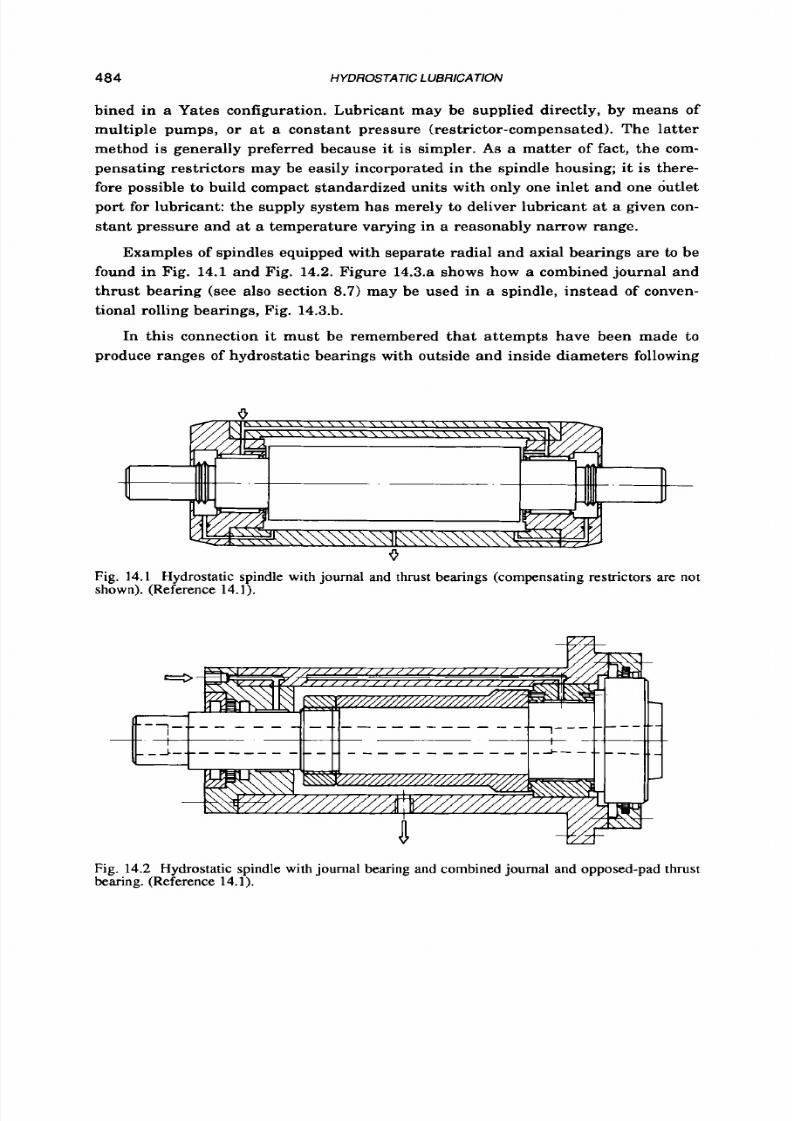
8/9/2019 Hydrostatic Lubrication 1992
http://slidepdf.com/reader/full/hydrostatic-lubrication-1992 501/558
484 HYDROSTATC LUBRlCATlON
bined in a Yates configuration. Lubricant may be supplied directly, by means of
multiple pumps, o r at a constant pressure (restrictor-compensated). The latter
method is generally preferred because it is simpler.
As
a matter of fact, the com-
pensating restrictors may be easily incorporated in the spindle housing; i t is there-
fore possible to build compact standardized units with only one inlet and one outlet
port for lubricant: the supply system has merely to deliver lubricant at a given con-
stant pressure and a t a temperature varying in a reasonably narrow range.
Examples of spindles equipped with separate radial and axial bearings are to be
found in Fig. 14.1 and Fig. 14.2. Figure 14.3.a shows how
a
combined journal and
thrust bearing (see also section 8.7) may be used in a spindle, instead of conven-
tional rolling bearings, Fig. 14.3.b.
In this connection it must be remembered that attempts have been made
t o
produce ranges of hydrostatic bearings with outside and inside diameters following
V
6
Fig.
14.1
Hydrostatic spindle with journal and thrust bearings (compensating restrictors are not
shown). (Reference 14.1).
U
Fig. 14.2 Hydrostatic spindle with journal bearing and combined journal and opposed-pad thrust
bearing. (Reference 14.1).
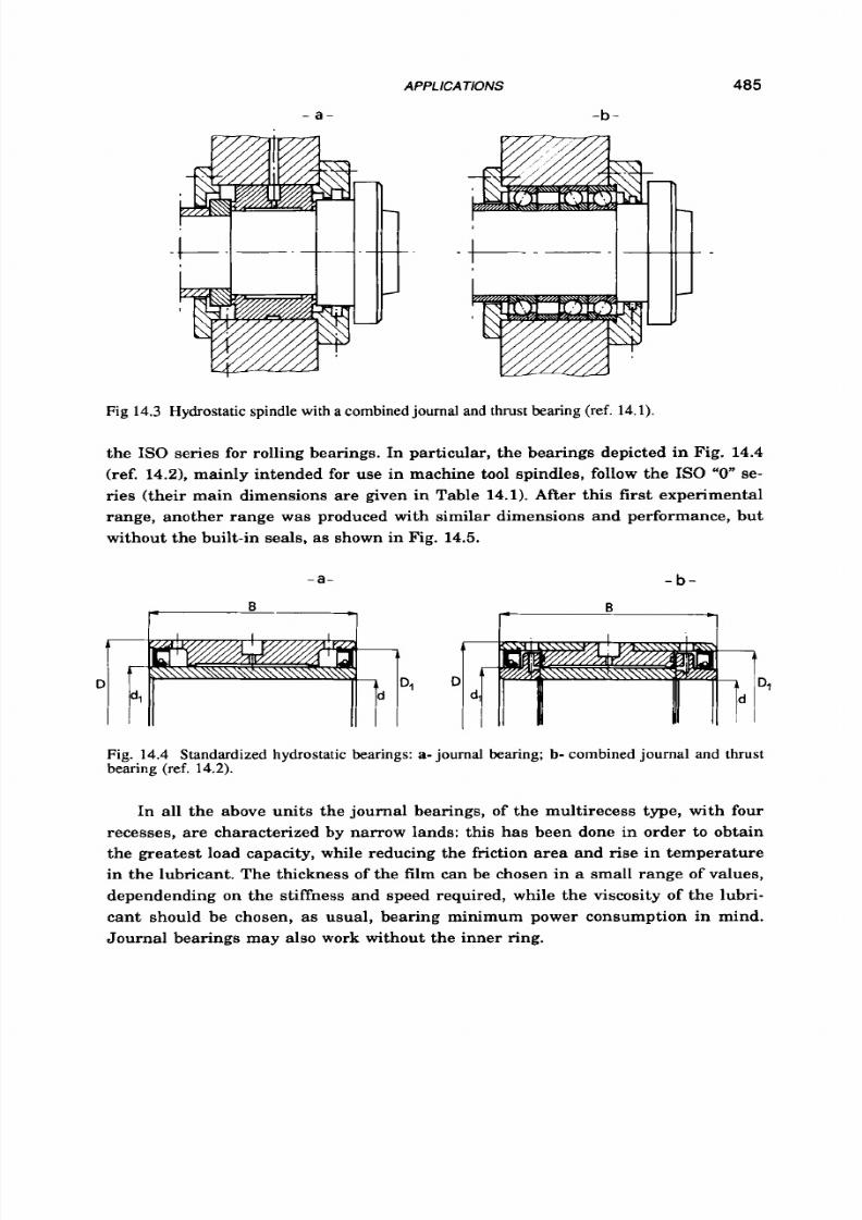
8/9/2019 Hydrostatic Lubrication 1992
http://slidepdf.com/reader/full/hydrostatic-lubrication-1992 502/558
APPL
/CATIONS
- a - -b-
485
Fig 14.3 Hydrostatic spindle with a combined journal and thrust bearing (ref. 14.1).
the
IS0
series for rolling bearings. In particular, the bearings depicted in Fig.
14.4
(ref.
14.21,
mainly intended
for
use in machine tool spindles, follow the
IS0
"0" se-
ries (their main dimensions are given in Table
14.1).
After this
first
experimental
range, another range was produced with similar dimensions and performance, but
without the built-in seals, as shown in Fig.
14.5.
- a - - b -
Fig. 14.4 Standardized hydrostatic bearings: a- journal bearing; b- combined journal and thrust
bearing (ref.
14.2).
In a ll the above units the journal bearings, of the multirecess type, with four
recesses, are characterized by narrow lands: this has been done in order to obtain
the greatest load capacity, while reducing the friction area and rise in temperature
in the lubricant. The thickness of the film can be chosen in a small range of values,
dependending on the stiffness and speed required, while the viscosity of the lubri-
cant should be chosen, as usual, bearing minimum power consumption in mind.
Journal bearings may also
work
without the inner ring.

8/9/2019 Hydrostatic Lubrication 1992
http://slidepdf.com/reader/full/hydrostatic-lubrication-1992 503/558
HYDROSTATIC LUBRICATlON
T A B L E
14.1
Standardized hydrostatic bearing un
(mm)
(mm)
(mm) (mm)
50
80
60 75
60 95 70
90
70 110
80
100
80
125 90
110
90
140
105 130
100 150
115
140
110 170 130 160
120 180
140 170
d
D
dl Dl
- a - -b-
(see Fig.
14.4).
B (mm)
Journal b. Combined b.
68 75
80 85
88 95
98
106
110 115
118 125
126 136
140 152
-C
-
Fig.
14.5
Standardized hydrostatic bearings:
a-
journal bearing; b- hrust bearing; c- combined
journal and thrust bearing (ref.
2.2).
Bearing un its ar e usually fed
at
constant pressure and for this reason can be
provided with laminar-flow restrictors, made up
of
a
stack of special discs fitted in
proper holes in the outer ring, very near the recesses of the bearing (Fig. 14.6.a).
These discs are
of
two types: one
is
plain with
a
hole in
its
centre, whereas the other
has
a
rectangular groove on both sides. Restriction
is
obtained in the grooves, since
they a re shallow (however, not less th an 80 pm). The total hydraulic resistance of
the restrictor may be changed by varying the number of stacked discs.
Another type of variable restrictor
is
shown in Fig. 14.6.b: in this case,
a
set-
screw is used to adjust the hydraulic resistance.
Bearings can also be feed a t
a
constant flow rate: this may be convenient espe-
cially for thru st bearings, in order to increase stiffness,
at
the cost of a slightly more
complicated supply system.
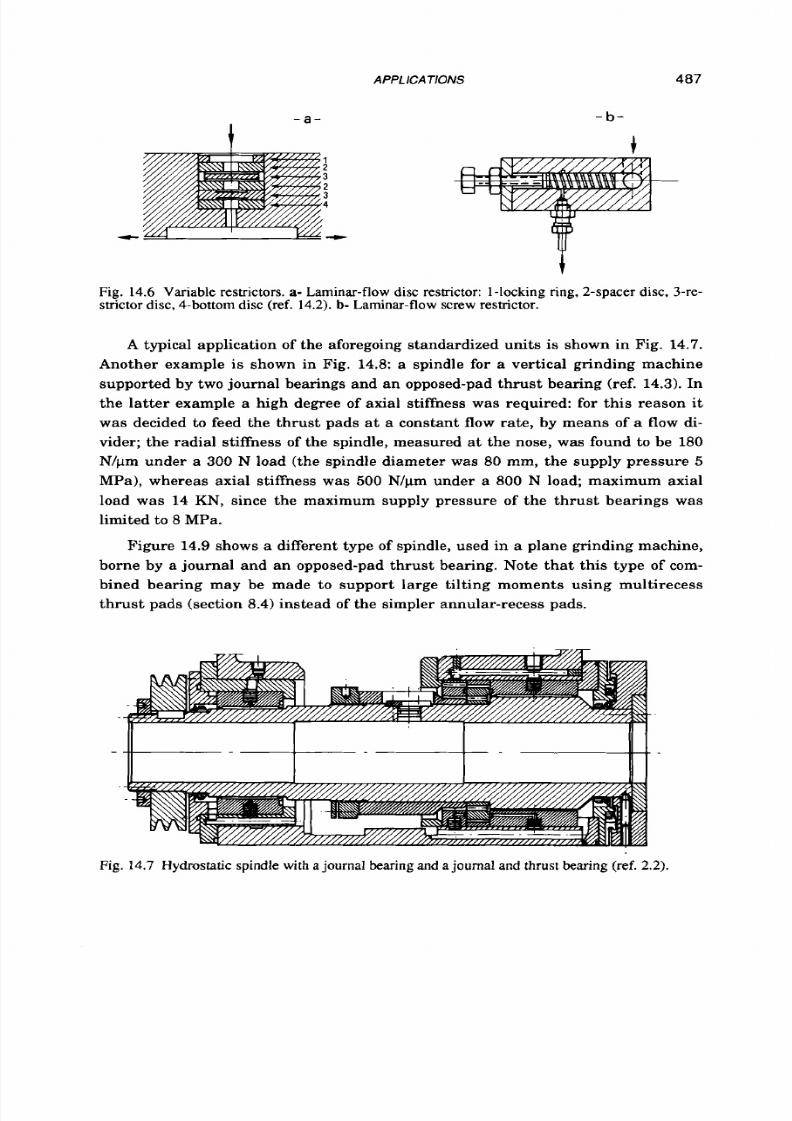
8/9/2019 Hydrostatic Lubrication 1992
http://slidepdf.com/reader/full/hydrostatic-lubrication-1992 504/558
- a -
t
APPLlCATlONS
- b -
487
1
2
3
2
3
4
.c
t
t
Fig. 14.6 Variable restrictors. a- Laminar-flow disc restrictor:
1
-locking ring, 2-spacer disc, 3-re-
strictor disc, 4-bottom disc
(ref.
14.2).
b-
Laminar-flow screw
restrictor.
A typical application of the aforegoing standardized units is shown in Fig. 14.7.
Another example is shown in Fig. 14.8: a spindle for a vertical grinding machine
supported by two journal bearings and an opposed-pad thrust bearing (ref. 14.3). In
the latter example a high degree of axial stiffness was required: for this reason it
was decided to feed the thrust pads at a constant flow rate, by means of a flow di-
vider; the radial stiffness of the spindle, measured a t the nose, was found to be 180
N/pm under a
300 N
oad (the spindle diameter was 80 mm, the supply pressure 5
MPa), whereas axial stiffness was 500 N/pm under a 800 N load; maximum axial
load was 14
KN,
since the maximum supply pressure of the thrust bearings was
limited to 8 MPa.
Figure 14.9 shows a different type of spindle, used in a plane grinding machine,
borne by a journal and an opposed-pad thrust bearing. Note that this type of com-
bined bearing may be made to support large tilting moments using multirecess
thrust pads (section 8.4) instead of the simpler annular-recess pads.
Fig. 14.7 Hydrostatic spindle w i t h a journal bearing and a journal and thrust bearing (ref. 2.2).
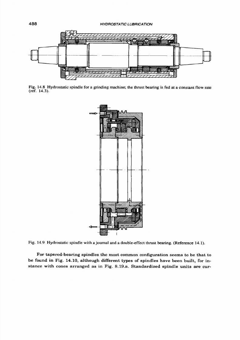
8/9/2019 Hydrostatic Lubrication 1992
http://slidepdf.com/reader/full/hydrostatic-lubrication-1992 505/558
488
HYDROSTATIC LUB RICATlON
E
Fig. 14.8 Hydrostatic spindle for a grinding machine; the thrust bearing is fed at a constant f low rate
(ref. 14.3).
Fig.
14.9
Hydrostatic spindle with a journal and a double-effect thrust bearing. (Reference 14.1).
For tapered-bearing spindles the most common configuration seems to be that to
be found in Fig. 14.10, although different types of spindles have been built, for in-
stance with cones arranged as in Fig. 8.19.a. Standardized spindle units are cur-

8/9/2019 Hydrostatic Lubrication 1992
http://slidepdf.com/reader/full/hydrostatic-lubrication-1992 506/558
A
PPLICA
TIQNS 489
Fig. 14 .10 Hydrostatic spindle with conical
bearings.
Ring
R
is used to adjust film thickness.
(Reference 14.1).
rently produced, which are interchangeable with rolling-bearing o r hydrodynamic
units produced by the same firm; of course, the main spindle dimensions comform
with international standards for machine tools (ref
14.4).
A n example of a standard spindle unit is shown in Fig.
14.11
nd the main rele-
vant data are to be found in Table 14.2 ref.
14.4).
L a -
Fig. 14.11 Standard spindle unit with cylindrical housing for boring, turning or milling (ref. 14.4).
Selection of the main hydrostatic parameters (number of recesses and their
dimensions, film thickness, lubricant viscosity and so on) is generally made case-
by-case by the manufacturer, on the basis of the operating conditions for which the
spindle is designed (mainly load and velocity) and also on the basis of particular
requirements, concerning stiffness and damping.
Comparing the data in Table 14.2with data concerning the equivalent spindle
units equipped with ball bearings (ref. 14.41,
t
should be noted tha t the hydrostatic
units show greater radial stiffness (although units equipped with special roller
bearings are much stiffer). It should be borne in mind, however, that the stiffness of
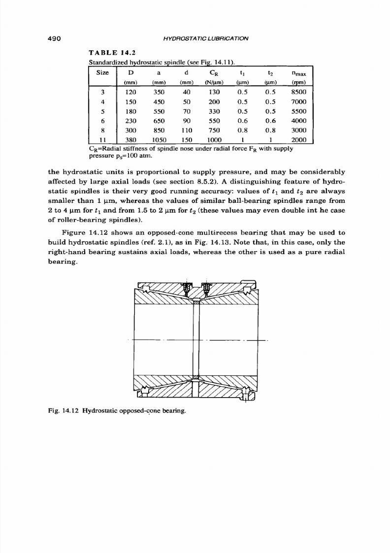
8/9/2019 Hydrostatic Lubrication 1992
http://slidepdf.com/reader/full/hydrostatic-lubrication-1992 507/558
4 9 0
Size
3
4
5
6
8
11
H Y D R O S T A X
LUBRlCATION
D a d CR
t l
t2 nmax
(mm) (mm)
(mm)
(W @m)
(rpm)
120 350 40 130
0.5
0.5 8500
150 450 50 200 0.5 0.5
7000
180 550 70
330
0.5 0.5 5500
230 650
90 550
0.6 0.6 4000
300
850 110
750 0.8 0.8 3000
380 1050 150
1000
1 1 2000
the hydrostatic units is proportional
t o
supply pressure, and may be considerably
affected by large axial loads (see section 8.5.2).A distinguishing feature of hydro-
static spindles is their very good running accuracy: values of t l and t 2 are always
smaller than
1
pm, whereas the values of similar ball-bearing spindles range from
2 t o 4
pm for
t l
and from
1.5 to 2
pm for
t 2
(these values may even double int he case
of
roller-bearing spindles).
Figure 14.12 shows an opposed-cone multirecess bearing that may be used t o
build hydrostatic spindles (ref. 2.11, as in Fig. 14.13. Note that , in this case, only the
right-hand bearing sustains axial loads, whereas the other is used as a pure radial
bearing.
Fig.
14.12
Hydrostatic opposed-cone
bearing.

8/9/2019 Hydrostatic Lubrication 1992
http://slidepdf.com/reader/full/hydrostatic-lubrication-1992 508/558
APPLICATIONS
491
Fig.
14.13
Hydrostatic spindle
with
a pair of opposed-cone bearings.
14.2.2
Steady rests
Mounting of long and heavy rotors (e.g. turbine rotors, steel mill rolls, calen-
ders, etc.) on lathes or other machine tools often requires the use of steady rests in
order
t o
relieve the headstock and tailstock spindles from excessive loads and t o
reduce the bending of the axis of the workpiece. On the other hand, conventional
steadies are characterized by high friction, with the relevant wearing and heating
of the rubbing surfaces: these problems can be completely eliminated by means of
hydrostatic lubrication.
A
steady for a heavy machine tool may easily be built with a couple of self-align-
ing shoes (ref. 14.5) f the type shown in section 14.3. ach shoe must be mounted on
a radially adjustable support to allow exact positioning of the workpiece.
In the application described in ref. 14.6, teadies for sustaining rubber-coated
cylinders (up to 600 KN in weight) on a grinding machine have been built. The
hydrostatic shoe is provided not only with a spherical seat allowing tilt in all direc-
tions, but also with a screw and nu t assembly for easily adjusting the radial position
of the shoe (Fig. 14.14). t should be noted that the intermediate piece of the bearing
is fitted in a hydraulic cylinder which is widened in the base piece; pressure in the
cylinder is the same as in the recess: in this way the fillets of the screw and nu t are
loaded with only a fraction of the force acting on the bearing. In this case the cylin-
der to be machined does not lean directly on the shoe bearings since intermediate
rings are fitted on the necks of the cylinder: the same steadies can hence be used
with different workpieces without needing to change the shoes, but using different
rings, all of which have the same external diameter.
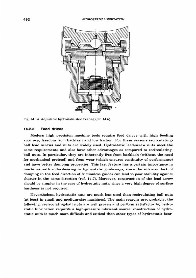
8/9/2019 Hydrostatic Lubrication 1992
http://slidepdf.com/reader/full/hydrostatic-lubrication-1992 509/558
492
HYDROSTATIC 1
UBRlCATION
Fig. 14.14 Adjustable hydrostatic shoe
bearing (ref.
14.6).
14.2.3
Feed drives
Modern high precision machine tools require feed drives with high feeding
accuracy, freedom from backlash and low friction. For these reasons recirculating-
ball lead screws and nuts are widely used. Hydrostatic lead-screw nuts meet the
same requirements and also have other advantages as compared to recirculating-
ball nuts. In particular, they are inherently free from backlash (without the need
for mechanical preload) and from wear (which ensures continuity of performance)
and have better damping properties. This last feature has a certain importance in
machines with roller-bearing or hydrostatic guideways, since the intrinsic lack of
damping in the feed direction of frictionless guides can lead to poor stability against
chatter in the same direction (ref. 14.7). Moreover, construction of the lead screw
should be simpler in the case of hydrostatic nuts, since a very high degree of surface
hardness
is
not required.
Nevertheless, hydrostatic nuts are much less used than recirculating ball nuts
(a t least in small and medium-size machines). The main reasons are , probably, the
following: recirculating-ball nuts are well proven and perform satisfactorily; hydro-
static lubrication requires a high-pressure lubricant source; construction of hydro-
static nuts is much more difficult and critical than other types of hydrostatic bear-
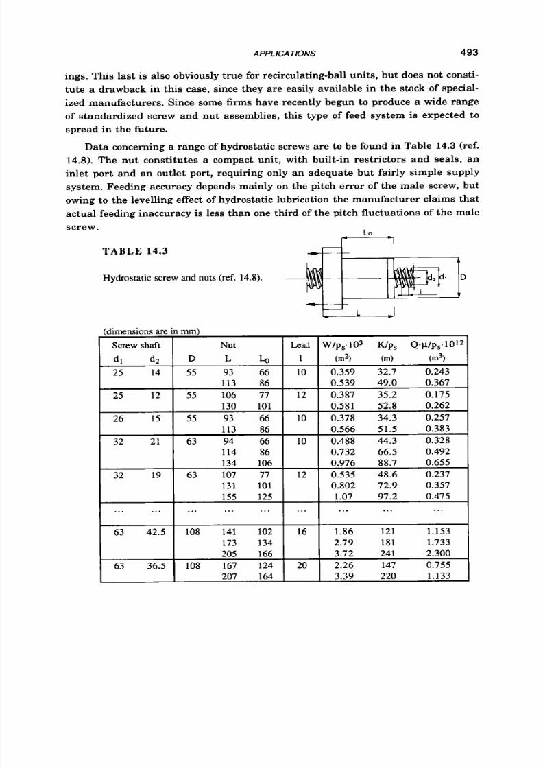
8/9/2019 Hydrostatic Lubrication 1992
http://slidepdf.com/reader/full/hydrostatic-lubrication-1992 510/558
APPLlCATlONS 493
63 36.5
ings. This last is also obviously true for recirculating-ball units, but does not consti-
tute a drawback in this case, since they are easily available in the stock of special-
ized manufacturers. Since some firms have recently begun to produce a wide range
of standardized screw and nut assemblies, this type
of
feed system
is
expected to
spread in the future.
Data concerning a range of hydrostatic screws are to be found in Table 14.3 ref.
14.8).
The nut constitutes a compact unit, with built-in restrictors and seals , an
inlet port and an outlet port, requiring only an adequate but fairly simple supply
system. Feeding accuracy depends mainly on the pitch error
of
the male screw, but
owing to the levelling effect
of
hydrostatic lubrication the manufacturer claims that
actual feeding inaccuracy is less than one third of the pitch fluctuations of the male
screw.
L o
T A B L E 14.3
Hydrostatic screw
and
nuts (ref.
14.8).
D
173 134 2.79
181 1.733
205
166
3.72
241 2.300
108 167 124
20 2.26
147 0.755
207 164 3.39 220 1.133
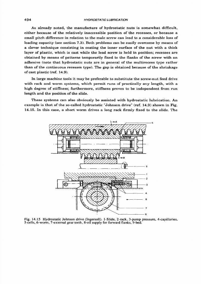
8/9/2019 Hydrostatic Lubrication 1992
http://slidepdf.com/reader/full/hydrostatic-lubrication-1992 511/558
494 HYDROSTATIC LUBRICATlON
As already noted, the manufacture of hydrostatic nuts is somewhat difficult,
either because of the relatively inaccessible position of the recesses, o r because a
small pitch difference in relation to the male screw can lead
to
a considerable loss of
loading capacity (see section
7.3).
Both
problems can be easily overcome by means of
a clever technique consisting in coating the inner surface
of
the nut with a thick
layer of plastic, which is cast while the lead screw is held in position; recesses are
obtained by means of patterns temporarily fixed
to
the flanks of the screw with an
adhesive (note that hydrostatic nuts are in general of the multirecess type rather
than of the continuous recesses type). The gap is obtained because of the shrinkage
of cast plastic (ref. 14.9).
In large machine tools it may be preferable to substitute the screw-nut feed drive
with rack and worm systems, which permit runs
of
practically any length, with a
high degree of stiffness; furthermore, stiffness proves t o be independent from run
length and the position of the slide.
These systems can also obviously be assisted with hydrostatic lubrication. An
example is tha t of the so-called hydrostatic "Johnson drive" (ref. 14.9) hown in Fig.
14.15. n this case, a short worm drives a long rack firmly fixed to the slide. The
Fig. 14.15 Hydrostatic Johnson drive (Ingersoll). 1-Slide, 2-rack, 3-pump pressure, 4-capillaries,
5-cells,
6-worm,
7-external gear teeth, 8-oil
supply
for forward flanks, 9-bed.
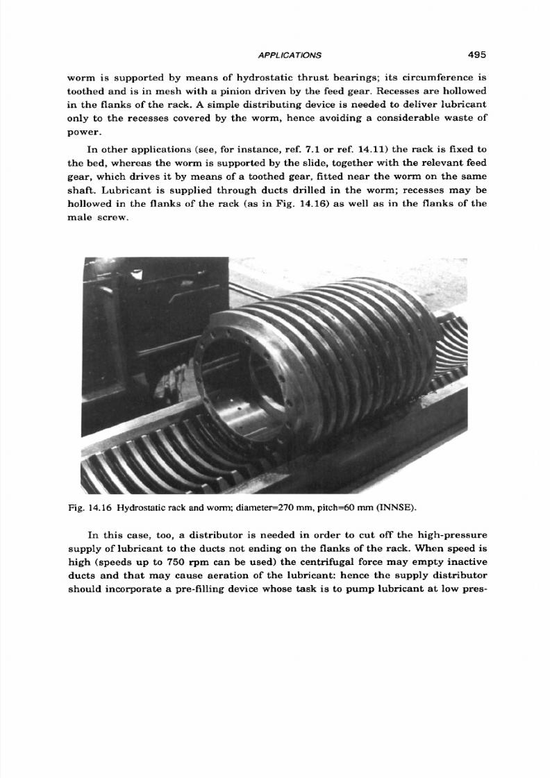
8/9/2019 Hydrostatic Lubrication 1992
http://slidepdf.com/reader/full/hydrostatic-lubrication-1992 512/558
A PPLICA TIONS
495
worm is supported by means of hydrostatic thrust bearings; its circumference is
toothed and is in mesh with a pinion driven by the feed gear. Recesses are hollowed
in the flanks of the rack. A simple distributing device is needed to deliver lubricant
only
t o
the recesses covered by the worm, hence avoiding a considerable waste
of
power.
In other applications (see, for instance, ref.
7.1
o r ref. 14.11) the rack is fixed t o
the bed, whereas the worm is supported by the slide, together with the relevant feed
gear, which drives it by means of a toothed gear, fitted near the worm on the same
shaft. Lubricant is supplied through ducts drilled in the worm; recesses may be
hollowed in the flanks of the rack (as in Fig. 14.16) s well as in the flanks of the
male screw.
Fig. 14.16 Hydrostatic rack and
worm;
iarnete-270 mm, itch=60 mm (INNSE).
In this case, too, a distributor is needed in order to cut off the high-pressure
supply of lubricant to the ducts not ending on the flanks of the rack. When speed is
high (speeds up to 750 rpm can be used) the centrifugal force may empty inactive
ducts and that may cause aeration of the lubricant: hence the supply distributor
should incorporate a pre-filling device whose task is to pump lubricant
at
low pres-

8/9/2019 Hydrostatic Lubrication 1992
http://slidepdf.com/reader/full/hydrostatic-lubrication-1992 513/558
496 HYDROSTATIC LUBRICA TlON
sure into the inactive ducts, just before they become active again (a similar device is
described in ref. 14.12).
Hydrostatic worms are generally built with a pitch of between
36 and 60
mm and
an outside diameter of between
150
and
300
mm; load capacity may vary between
50
and
180 KN.
The rack may be of virtually any length since
it
is built in sections (for
instance, 1000 mm in length) that are bonded and firmly bolted to the slide bed after
having been adjusted in relation to one another and measured to verify the pitch
error (ref. 7.1). Accuracy may be about 70i-80 pm on a length of 25 m. Owing t o this
accuracy and to the very high degree of stiffness this feed system can also be used
for monitoring the position of the slide during normal operation (by means of elec-
tronic compensation the relevant error can be further reduced to a very small
value).
14.2.4 Guideways and rotat ing tables
Hydrostatic lubrication proves to be particularly suitable
for
guideways
of
mod-
ern high precision machine tools (especially those equipped with numerical con-
trol), because of their intrinsic characteristics:
very low friction (and proportional to speed);
freedom from stick-slip;
freedom from wear (which means constancy of performance for an indefi-
nite time);
thickness of the oil film independent of the sliding speed (whereas for lubri-
cated plain bearings it increases with speed);
high damping capacity fin directions perpendicular to guide);
levelling ability: the fairly high film thickness (commonly a few hundredths
of
a
millimeter) allows the hydrostatic lubrication to compensate, a t least
partially,
for
small geometric inaccuracies and deformations
of
the guides;
possibility of building guides of virtually any length (which is difficult with
roller guides).
On the other hand, it should be noted that the virtual elimination of friction can
enhance the effects of the flexibility of other parts of the machine and in particular
of the feed drive. For instance, consider the experimental diagrams in Fig.
14.17
(see ref.
14.13
for further details): they refer to a milling machine and show that the
displacement due to loading in the direction of the guides (mainly due to the flexibil-
ity of the ball screw and nut and of the relevant thrust bearing) is greatly reduced by
the friction of the sliding ways.
Diagrams in Fig.
11.18
(ref.
14.71,
obtained with a similar experimental rig,
show the reduction in damping connected with the use of frictionless guides (either
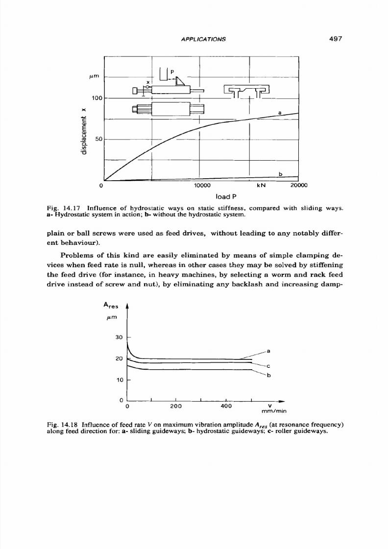
8/9/2019 Hydrostatic Lubrication 1992
http://slidepdf.com/reader/full/hydrostatic-lubrication-1992 514/558
APPLlCATlONS
497
0
10000 kN 20000
load
P
Fig. 14.17 Influence of hydrostatic ways on static stiffness, compared with sliding ways.
a-
Hydrostatic system
in
action; b- without the hydrostatic system.
plain or ball screws were used
as
feed drives, without leading to any notably differ-
en t behaviour).
Problems of this kind are easily eliminated by means of simple clamping de-
vices when feed rate
is
null, whereas in other cases they may be solved by stiffening
th e feed drive (for instance, in heavy machines, by selecting a worm and rack feed
drive instead of screw an d nut), by eliminating any backlash a nd increasing damp-
I I I I
I
*
0 200
400 V
mmlmin
Fig. 14.18 Influence of feed rate
V
on maximum vibration amplitudeA (at resonance frequency)
along feed direction for: a- sliding guideways; b- hydrostatic guideways; c - roller guideways.
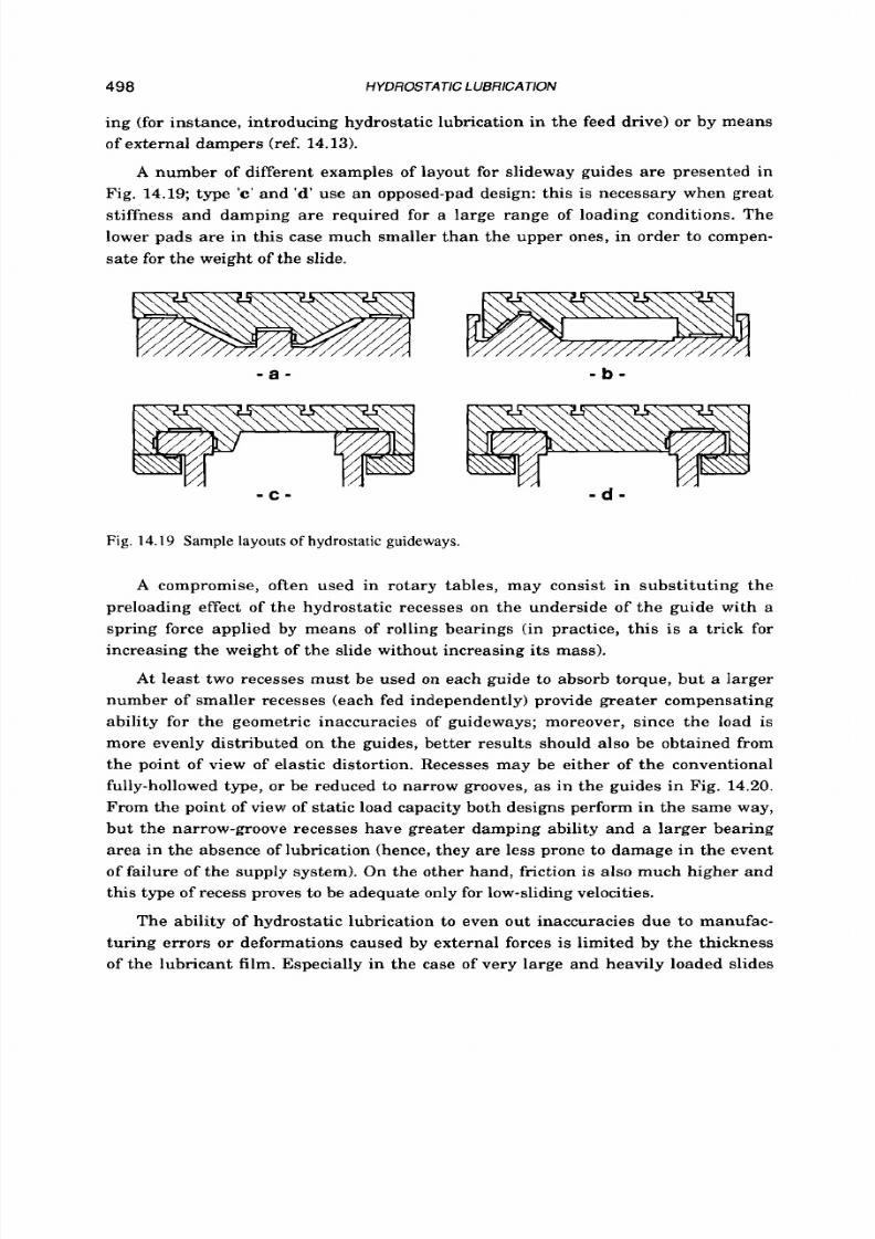
8/9/2019 Hydrostatic Lubrication 1992
http://slidepdf.com/reader/full/hydrostatic-lubrication-1992 515/558
498 HYDROSTATIC LUBRICATION
ing (for instance, introducing hydrostatic lubrication in the feed drive) or by means
of external dampers (ref. 14.13).
A number of different examples of layout for slideway guides are presented in
Fig.
14.19;
type
‘c ’
and
‘d‘
use an opposed-pad design: this
is
necessary when great
stiffness and damping are required for a large range of loading conditions. The
lower pads a re in this case much smaller th an t he upper ones, in order to compen-
sa te for th e weight of the slide.
- a -
- b -
- c - - d -
Fig.
14.19
Sample
layouts
of
hydrostatic guideways.
A compromise, often used in rotary tables, may consist in substituting the
preloading effect of the hydrostatic recesses on the underside of the guide with a
spring force applied by means of rolling bearings (in practice, this is a trick for
increasing the weight of the slide without increasing
its
mass).
At least two recesses must be used on each guide
to
absorb torque, but a larger
number of smaller recesses (each fed independently) provide greater compensating
ability for the geometric inaccuracies of guideways; moreover, since the load is
more evenly distributed on the guides, better results should also be obtained from
the point of view of elastic distortion. Recesses may be either of the conventional
fully-hollowed type,
or
be reduced to narrow grooves,
as
in the guides in Fig.
14.20.
From the point of view of static load capacity both designs perform in the same way,
but the narrow-groove recesses have greater damping ability and a larger bearing
area in the absence of lubrication (hence, they a re less prone t o damage in th e event
of failure of the supply system). On the other hand, friction is also much higher and
this type of recess proves to be adequate only for low-sliding velocities.
The ability of hydrostatic lubrication to even out inaccuracies due to manufac-
turing errors or deformations caused by external forces is limited by the thickness
of the lubricant film. Especially in the case of very large and heavily loaded slides
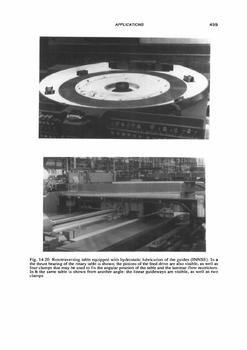
8/9/2019 Hydrostatic Lubrication 1992
http://slidepdf.com/reader/full/hydrostatic-lubrication-1992 516/558
APPLlCA
TlONS
499
Fig.
14.20
Rototraversing table equipped with hydrostatic lubrication of the guides
(INNSE).
In
a
the thrust bearing of the rotary table
is
shown; the pinions of the feed drive are also visible, a s well as
four clamps that may be used to
fix
the angular position of the table and the lam inar-flow restrictors.
In b the same table is shown from another angle: the linear guideways are visible, as well as two
clamps.
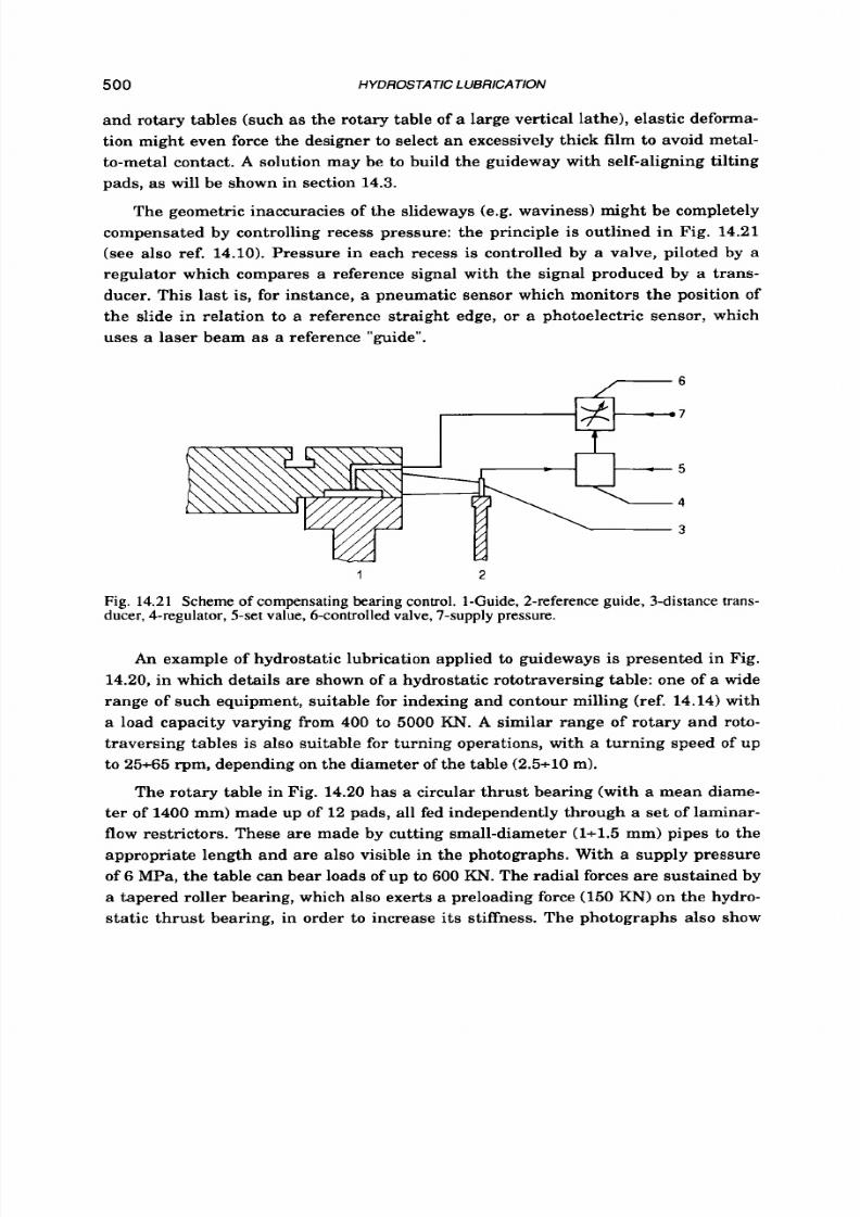
8/9/2019 Hydrostatic Lubrication 1992
http://slidepdf.com/reader/full/hydrostatic-lubrication-1992 517/558
500
HYDROSTATIC LUBRICATION
and rotary tables (such as the rotary table of a large vertical lathe), elastic deforma-
tion might even force the designer to select an excessively thick film to avoid metal-
to-metal contact. A solution may be to build the guideway with self-aligning tilting
pads, as will be shown in section
14.3.
The geometric inaccuracies of the slideways (e.g. waviness) might be completely
compensated by controlling recess pressure: the principle is outlined i n Fig. 14.21
(see also ref.
14.10).
Pressure in each recess is controlled by a valve, piloted by a
regulator which compares a reference signal with the signal produced by a trans-
ducer. This last is, for instance, a pneumatic sensor which monitors the position of
the slide in relation to
a
reference straight edge,
o r a
photoelectric sensor, which
uses a laser beam as a reference "guide".
1 2
Fig. 14.21 Scheme of compensating bearing
control.
1-Guide, 2-reference guide, 3-distance trans-
ducer, 4-regulator, 5-set value, 6-controlledvalve, 7-supply pressure.
A n example of hydrostatic lubrication applied to guideways is presented in Fig.
14.20,
n which details are shown of a hydrostatic rototraversing table: one of a wide
range of such equipment, suitable for indexing and contour milling (ref.
14.14)
with
a load capacity varying from
400
to
5000
KN.
A
similar range of rotary and roto-
traversing tables
is
also suitable for turning operations, with
a
turning speed of up
to 2565 pm, depending on the diameter of the table (2.5+10m).
The rotary table in Fig.
14.20
has a circular thrust bearing (with a mean diame-
ter of
1400
mm) made up of
12
pads, all fed independently through a set of laminar-
flow restrictors. These are made by cutting small-diameter (111.5mm) pipes t o the
appropriate length and are also visible in the photographs. With
a
supply pressure
of
6
MPa, the table can bear loads of up to 600 KN. The radial forces are sustained by
a tapered roller bearing, which also exerts a preloading force (150KN) on the hydro-
static thrust bearing, in order
t o
increase its stiffness. The photographs also show
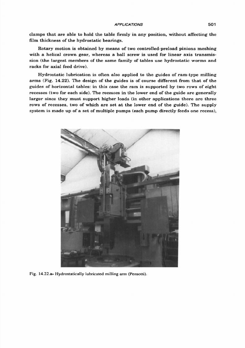
8/9/2019 Hydrostatic Lubrication 1992
http://slidepdf.com/reader/full/hydrostatic-lubrication-1992 518/558
APPL
ICATlONS 501
clamps that are able to hold the table firmly in any position, without affecting the
film thickness of the hydrostatic bearings.
Rotary motion is obtained by means of two controlled-preload pinions meshing
with a helical crown gear, whereas a ball screw
is
used for linear axis transmis-
sion (the largest members of the same family of tables use hydrostatic worms and
racks for axial feed drive).
Hydrostatic lubrication is often also applied to the guides of ram-type milling
arms (Fig.
14.22).
The design of the guides is of course different from that of the
guides of horizontal tables: in this case the ram
is
supported by two rows of eight
recesses (two for each side). The recesses in the lower end of the guide are generally
larger since they must support higher loads (in other applications there are three
rows of recesses, two of which are set
at
the lower end of the guide). The supply
system is made up of a set of multiple pumps (each pump directly feeds one recess),
Fig. 14.22.a-Hydrostatically lubricated milling
arm
Pensotti).

8/9/2019 Hydrostatic Lubrication 1992
http://slidepdf.com/reader/full/hydrostatic-lubrication-1992 519/558
502
HYDROSTATC LUBRlCAT/ON
Fig. 14.22.b-
Hydrostatically lubricated milling
arm:
etail showing hydrostatic pads.
which are fed
at
constant pressure
(-2.5
MPa) by a larger pump. In this case, too,
the recesses of the pads (which are made of bronze) are reduced to narrow grooves.
It is
interesting that hydrostatic lubrication has also been used to compensate
for the deflection of the ram due
t o
the cutting force. The geometric adaptive control
system described in ref.
14.15
measures the displacement of the milling head by
means of a laser gun fixed
t o
the milling arm, which emits a laser beam parallel
t o
the undeformed axis of the ram, and a photoelectric scanner attached
t o
the milling
head. The signal produced by the measuring equipment is taken as its input by a
control unit which varies accordingly the speed of a servo-motor driving a further
set of pumps. The
flow
produced by these compensating pumps
is
directed towards
the appropriate recesses and added
t o
the normal flow in order to produce a dis-
placement of the milling head, realigning it with the laser beam.
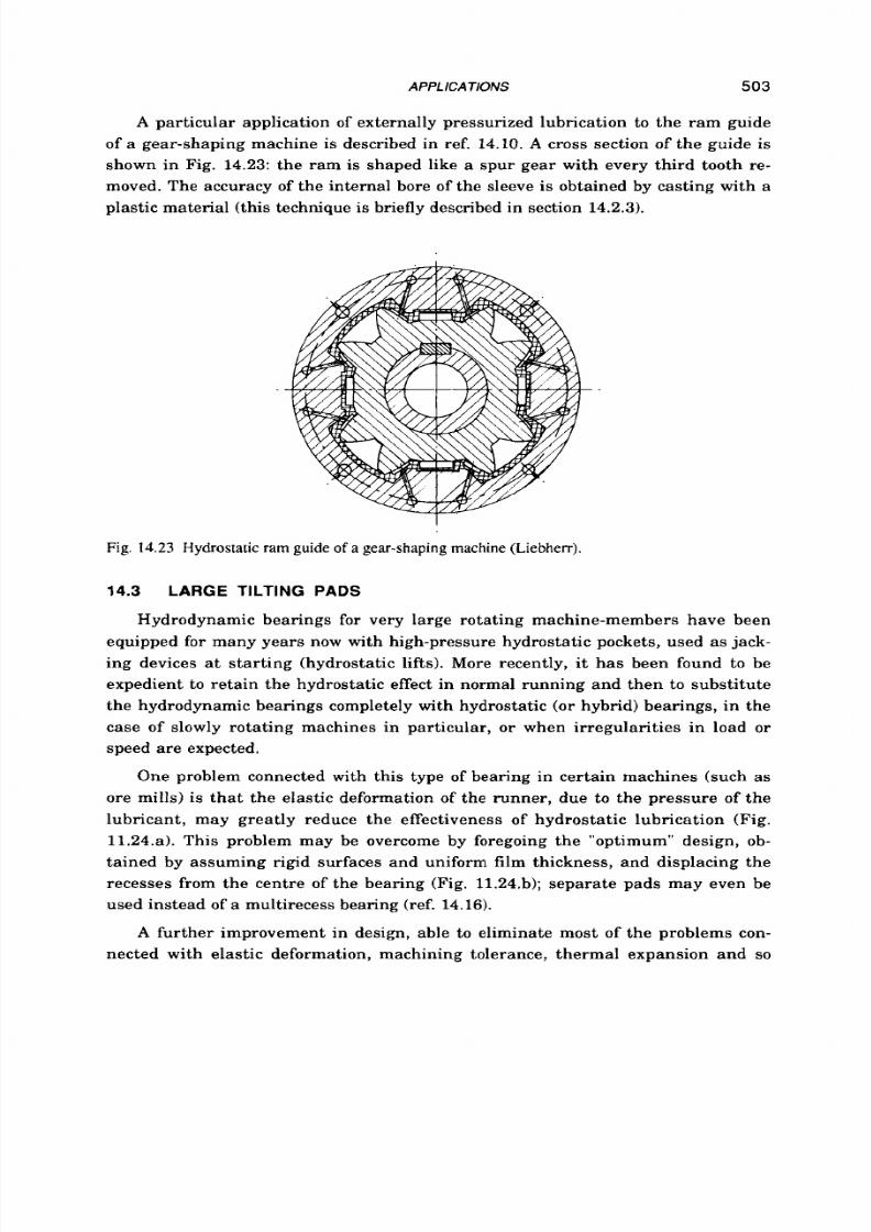
8/9/2019 Hydrostatic Lubrication 1992
http://slidepdf.com/reader/full/hydrostatic-lubrication-1992 520/558
A
P P l
CA TlONS
503
A particular application of externally pressurized lubrication to the ram guide
of
a
gear-shaping machine is described in ref. 14.10.
A
cross section of the guide is
shown in Fig. 14.23: the ram is shaped like a spur gear with every third tooth re-
moved. The accuracy of the internal bore of the sleeve is obtained by casting with a
plastic material (this technique is briefly described in section 14.2.3).
Fig.
14.23
Hydrostatic ram guide of a gear-shaping machine (Liebherr).
14.3
LARGE
TILTING PADS
Hydrodynamic bearings for very large rotating machine-members have been
equipped fo r many years now with high-pressure hydrostatic pockets, used as jack-
ing devices
at
starting (hydrostatic lifts). More recently, it has been found t o be
expedient to retain the hydrostatic effect in normal running and then t o substitute
the hydrodynamic bearings completely with hydrostatic (or hybrid) bearings, in the
case of slowly rotating machines in particular, or when irregularities in load
o r
speed are expected.
One problem connected with this type of bearing in certain machines (such as
ore mills) is that the elastic deformation of the runner, due to the pressure of the
lubricant, may greatly reduce the effectiveness
of
hydrostatic lubrication (Fig.
11.24.a). This problem may be overcome by foregoing the "optimum" design, ob-
tained by assuming rigid surfaces and uniform film thickness, and displacing the
recesses from the centre of the bearing (Fig. 11.24.b); separate pads may even be
used instead
of a
multirecess bearing (ref. 14.16).
A further improvement in design, able t o eliminate most of the problems con-
nected with elastic deformation, machining tolerance, thermal expansion and so

8/9/2019 Hydrostatic Lubrication 1992
http://slidepdf.com/reader/full/hydrostatic-lubrication-1992 521/558
504
HYDROSTATIC
LUBRICATlON
Fig. 14.24 Trunnion deformation due to bearing pressure: a- bearing
as
designed;
b-
improved
concept; e- most effective concept (ref. 14.16).
on, consists in supporting the large journal by means of a set of self-aligning hydro-
static shoes, as shown in Fig. 14.25 (ref.
14.17).
Each shoe is split up into t w o parts:
the upper part rests on a spherical seat and hence can tilt in all directions. The
underside of the upper part is shaped like a piston which fits into a cylinder in the
base: since the piston area, on which the recess pressure acts, is slightly smaller
than the effective area of the pad, the load on the spherical seat is quite low during
normal operation.
Fig. 14.25 Arrangement of tilting-pad hydrostatic bearings (ref. 14.17).

8/9/2019 Hydrostatic Lubrication 1992
http://slidepdf.com/reader/full/hydrostatic-lubrication-1992 522/558
APPLICATIONS
505
The spherical rest of each inner shoe (slave shoe) is pushed against the runner
by a further piston on which, thanks to a hydraulic connection, the recess pressure
of the relevant outer shoe (master shoe) acts. Clearly, if the sum of the two piston
areas equals the effective pad area, the slave shoe must necessarily have the same
film thickness, and thus the same recess pressure, as the relevant master shoe
(each pad is fed by the same flow rate). Thus when the load direction is vertical all
four shoes have the same film thickness and recess pressure, regardless of the
deviation
of
the runner from the ideal circular shape. When the load deviates from
the vertical direction the
two
shoes on each side have an equal part of the load com-
ponent falling along the line between the two shoes (ref. 14.17).
The shape of the recess is also of particular interest. It is known that when a
cylindrical pad with a simple recess
(as
in Fig.
5.30)
s
tilted from the concentric
configuration the pressure field on the land surface is altered and produces a
moment that tends to realign the pad; however, this self-aligning capacity
is
too
small to ensure the stability of the shoe in all conditions and i t is hence necessary to
use multirecess pads. In Fig. 14.26 he main recess is surrounded by four auxiliary
recesses, situated in the corners of the pad, which are fed with the lubricant which
passes from the central recess over the bearing lands and through small drilled
ducts (this is a compromise aimed at avoiding dependence upon the direction of
rotation: for the greatest stability the auxiliary recesses on the trailing side should
only be supplied over the lands).
The hydrostatic system described in ref. 14.17 upported a large tube mill for
crushing ores: each bearing runner had a diameter of 2700 mm, the maximum
I
I
L
-
Fig. 14.26 Improved recess pattern (ref. 14.17).
W
.
I

8/9/2019 Hydrostatic Lubrication 1992
http://slidepdf.com/reader/full/hydrostatic-lubrication-1992 523/558
506 HYDROSTA
T C
LUBRlCA
T/ON
load was
3500 KN
and the velocity was 0.24 re ds . Each shoe was 640 mm long and
500
mm wide and was fed at 25 Ym with a lubricant whose viscosity was 0.1 Ns/m2
at 50°C. Film thickness in normal operation was 0.1410.15 111111.
A range of hydrostatic shoes based on the foregoing working principles is cur-
rently produced by the same firm (ref. 14.5): a sketch of them i s to be found in Fig.
14.27 and their main dimensions are given in table 14.4. The recess patte rn is simi-
lar t o that shown in Fig. 14.26, but the main recess is now annular in shape, in
order t o increase the bearing area a t rest ( in the absence of hydrostatic lubrication)
virtually without affecting bearing performance during normal operation.
Hydrostatic shoes may be used to support horizontal as well as vertical rotating
equipment. In the first case the rotating drum may lean on the shoes by means of
trunnions (Fig. 14.28.a) or by means of girth rings (Fig. 14.28.b). The lat ter a r-
rangement, which is often inapplicable with rolling bearings due to their size lim-
its, permits large feed openings and a simplified (and less expensive) design. Each
- a - - b -
Fig.
14.27
Bearing shoes:
a-
master shoe; b- slave shoe.
T A B L E 1 4 . 4
410
530
SO0 640
600 756
H
(mm)
Master
Slave
180+190
2601270
300 2951305
320+330
425 4201430
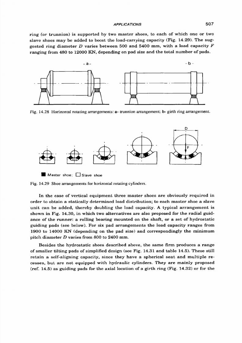
8/9/2019 Hydrostatic Lubrication 1992
http://slidepdf.com/reader/full/hydrostatic-lubrication-1992 524/558
APPLlCA
TlONS
507
ring (or trunnion)
is
supported by two master shoes, to each of which one or two
slave shoes may be added
t o
boost the load-carrying capacity (Fig.
14.29).
The sug-
gested ring diameter D varies between 500 and 5400 mm, with a load capacity F
ranging from
480
t o
12000
KN,
depending on pad size and the total number of pads.
- a - - b -
Fig.
14.28
Horizontal rotating arrangements: a-
trunnion
arrangement;
b-
girth ring arrangement.
D
as ter s hoe: O S l a v e s hoe
Fig.
14.29
Shoe arrangements
for
horizontal rotating cylinders.
In the case of vertical equipment three master shoes are obviously required in
order
t o
obtain a statically determined load distribution; t o each master shoe a slave
unit can be added, thereby doubling the load capacity. A typical arrangement is
shown in Fig. 14.30, in which two alternatives are also proposed for the radial guid-
ance of the runner: a rolling bearing mounted on the shaft, or a set of hydrostatic
guiding pads (see below). For six pad arrangements the load capacity ranges from
1900 t o 14000 KN (depending on the pad size) and correspondingly the minimum
pitch diameter D varies from 800 to 2400 mm.
Besides the hydrostatic shoes described above, the same firm produces a range
of smaller tilting pads of simplified design (see Fig. 14.31 and table 14.5).These still
retain
a
self-aligning capacity, since they have a spherical seat and multiple re-
cesses, but are not equipped with hydraulic cylinders. They are mainly proposed
(ref. 14.5) as guiding pads for the axial location of
a
girth ring (Fig. 14.32) o r for the
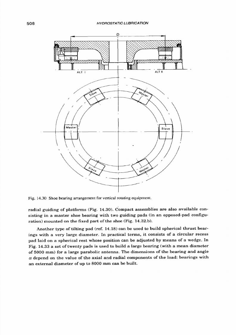
8/9/2019 Hydrostatic Lubrication 1992
http://slidepdf.com/reader/full/hydrostatic-lubrication-1992 525/558
508
HYDROSTATIC LUBRICATION
r
D
ALT
II
I
L T I
Fig.
14.30
Shoe bearing arrangement
for
vertical rotating equipment.
radial guiding of platforms (Fig. 14.30). Compact assemblies are also available con-
sisting in a master shoe bearing with t w o guiding pads (in an opposed-pad configu-
ration) mounted on the fixed part
of
the shoe (Fig. 14.32.b).
Another type of tilting pad (ref. 14.18) can be used t o build spherical th rust bear-
ings with
a
very large diameter. In practical terms, it consists
of
a circular recess
pad laid on a spherical rest whose position can be adjusted by means
of
a wedge. In
Fig. 14.33 a set
of
twenty pads is used
t o
build
a
large bearing (with a mean diameter
of
5000 mm) for a large parabolic antenna. The dimensions of the bearing and angle
a depend on the value of the axial and radial components of the load: bearings with
an external diameter of up t o
8000
mm can be built.

8/9/2019 Hydrostatic Lubrication 1992
http://slidepdf.com/reader/full/hydrostatic-lubrication-1992 526/558
APPLlCATlONS
Fig. 14.31 Guiding pad.
509
T A B L E
14.5
Dimensions of guiding pads (ref. 14.5).
Fig. 14.32 Axial guiding pads: a- separate axial guidance; b- axial guidance integral with a master
shoe.
A further type of tilting shoe is shown in Fig. 14.34 ref. 14.19): t can ti lt around
the cylindrical rib on the underside and align itself thanks to the multiple recesses
(two o r four) which are fed independently through capillary restrictors. These pads
can
a lso
be used to sustain radial loads as well as the axial thrust of a large rotating
platform. In the latter case, bearings with diameters exceeding 5000 mm may be
built, which sustain thrusts greater than 5000 KN and rotating at more than 20
rpm. These pads prove t o be particularly suitable for building rotary tables for large
machine tools (e.g. for vertical lathes): an example is given in Fig.
14.35.
A different
application
is
described in ref.
14.20,
oncerning the supporting ring of a
3.5
m
telescope.
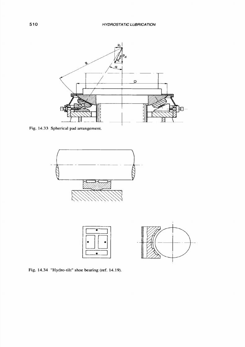
8/9/2019 Hydrostatic Lubrication 1992
http://slidepdf.com/reader/full/hydrostatic-lubrication-1992 527/558
510
HYDROSTATIC LUBRICATION
P I
Fig. 14 .33 Spherical pad arrangement,
Fig. 14.34 "Hydro-tilt"shoe bearing (ref. 14.19).

8/9/2019 Hydrostatic Lubrication 1992
http://slidepdf.com/reader/full/hydrostatic-lubrication-1992 528/558
APPLlCA TlONS
511
Fig. 14.35 "Hydro-tilt" shoe
arrangement.
Lastly, Fig. 14.36 shows a large-size spherical bearing (ref. 2.2); it has three
recesses fed a t a constant
flow
rate. Bearings like this can sustain heavy loads (up to
10,000 KN) and in general their rotating speed is low.
For
instance, the bearing
depicted
in
Fig. 14.36 was made
to
support the rotor
of
an air preheater weighing
800
KN
and rotating at 2 rpm.
14.4 OTHER APPLICATIONS
Apart from those quoted in the foregoing sections, hydrostatic lubrication has a
number of different applications.
For
instance, let
us
consider the pump in Fig. 14.37 (ref. 14.21): the pistons (1)
lean on the tilted plate (2) by means of the spherical pads (3) which are hydrostati-
cally borne by the same circulating fluid.
Another special application is quoted in ref. 14.22, that is the lower journal bear-
ing of the main pump
of
the Super-PhBnix nuclear power plant. This bearing has a
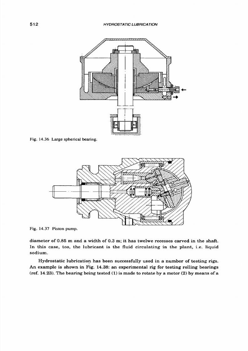
8/9/2019 Hydrostatic Lubrication 1992
http://slidepdf.com/reader/full/hydrostatic-lubrication-1992 529/558
512
HYDROSTATIC L UBRICATlON
L . L . 1
r ' t ' i
Fig. 14.36 Large sphericalbearing.
Fig.
14.37
Piston
pump.
diameter of 0.85 m and a width
of
0.3m; it has twelwe recesses carved in the shaft.
In this case, too, the lubricant is the fluid circulating in the plant, i.e. liquid
sodium.
Hydrostatic lubrication has been successfully used in a number
of
testing rigs.
An example
is
shown in Fig. 14.38:an experimental rig for testing rolling bearings
(ref. 14.23).The bearing being tested (1) is made t o rotate by a motor (2) y means of a
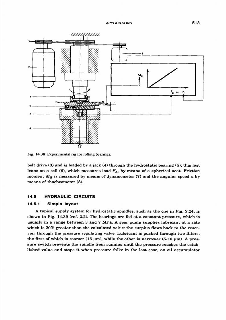
8/9/2019 Hydrostatic Lubrication 1992
http://slidepdf.com/reader/full/hydrostatic-lubrication-1992 530/558
APPLICATIONS
513
Fig.
14.38 Experimental
rig
for rolling bearings.
belt drive
(3)
and is loaded by a jack (4) through the hydrostatic bearing (5); his last
leans on a cell
(61,
which measures load
Fa,
by means of
a
spherical seat. Friction
moment
MR
s measured by means of dynamometer
(7)
nd the
angular
speed
n
by
means of thacheometer
(8).
14.5 HYDRAULIC
CIRCUITS
14.5.1 Simple layout
A
typical supply system for hydrostatic spindles, such
as
the one in Fig.
2.24,
is
shown in Fig.
14.39 (ref.
2.2).
The bearings are fed
at
a constant pressure, which is
usually in a range between
3 and 7 MPa. A gear pump supplies lubricant
at
a rate
which is 30% greater than the calculated value: the
surplus
flows back to the reser-
voir through the pressure regulating valve. Lubricant is pushed through two filters,
the first of which
is
coarser
(15
pm), while the other
is
narrower
(5-10
m).
A
pres-
sure switch prevents the spindle from running until the pressure reaches the estab-
lished value and stops it when pressure falls: in the last case,
an
oil accumulator
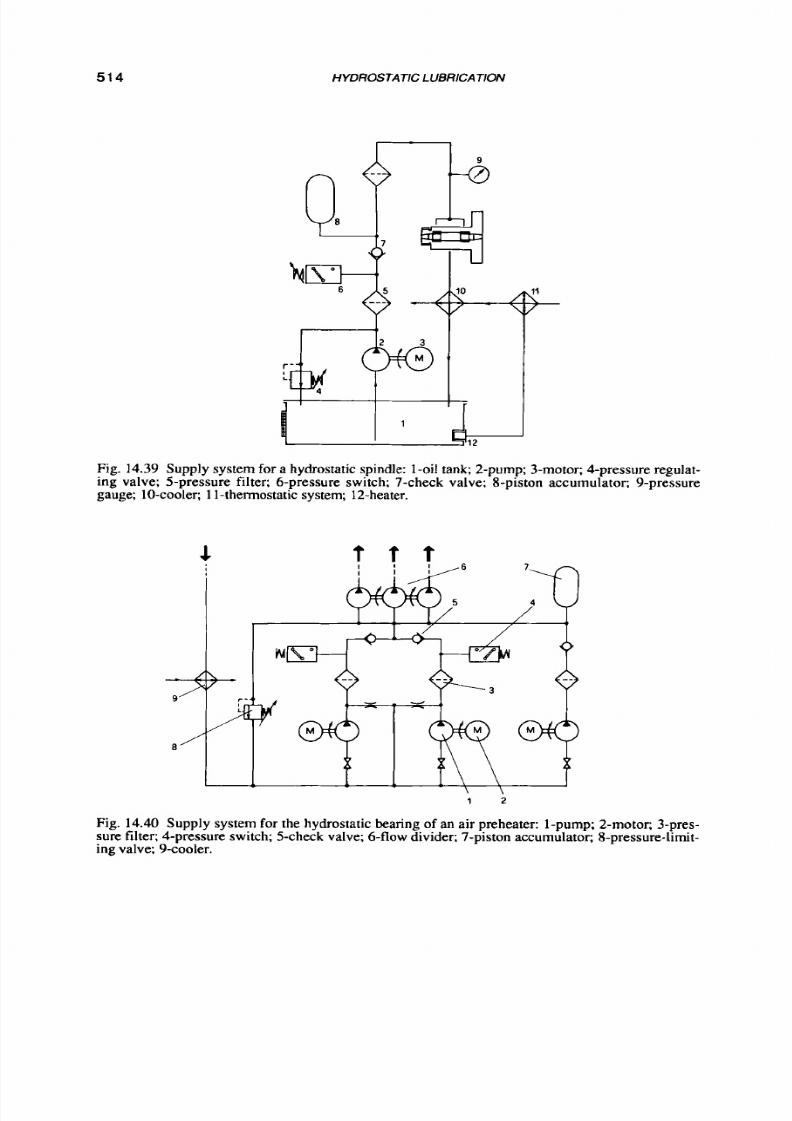
8/9/2019 Hydrostatic Lubrication 1992
http://slidepdf.com/reader/full/hydrostatic-lubrication-1992 531/558
514
HYDROSTATIC LUBRICATION
Fig. 14.39 Sup ply system for a hydrostatic spindle: 1-oil tank; 2-pum p; 3-motor; 4-pre ssure regulat-
ing valve; 5-pressure filter; 6-pressure switch; 7-check valve; 8-piston accumulator; 9-pressure
gauge; 10-cooler;
1
1-thermostaticsystem; 12-heater.
1 2
Fig. 14.40 Supply system for the hydrostatic bearing of
an
air preheater: 1-pum p; 2-motor; 3-pres-
sure filter; 4-pressure switch; 5-check valve; 6-flow divider; 7-piston accum ulator; 8-pressure-limit-
ing valve; 9-cooler.
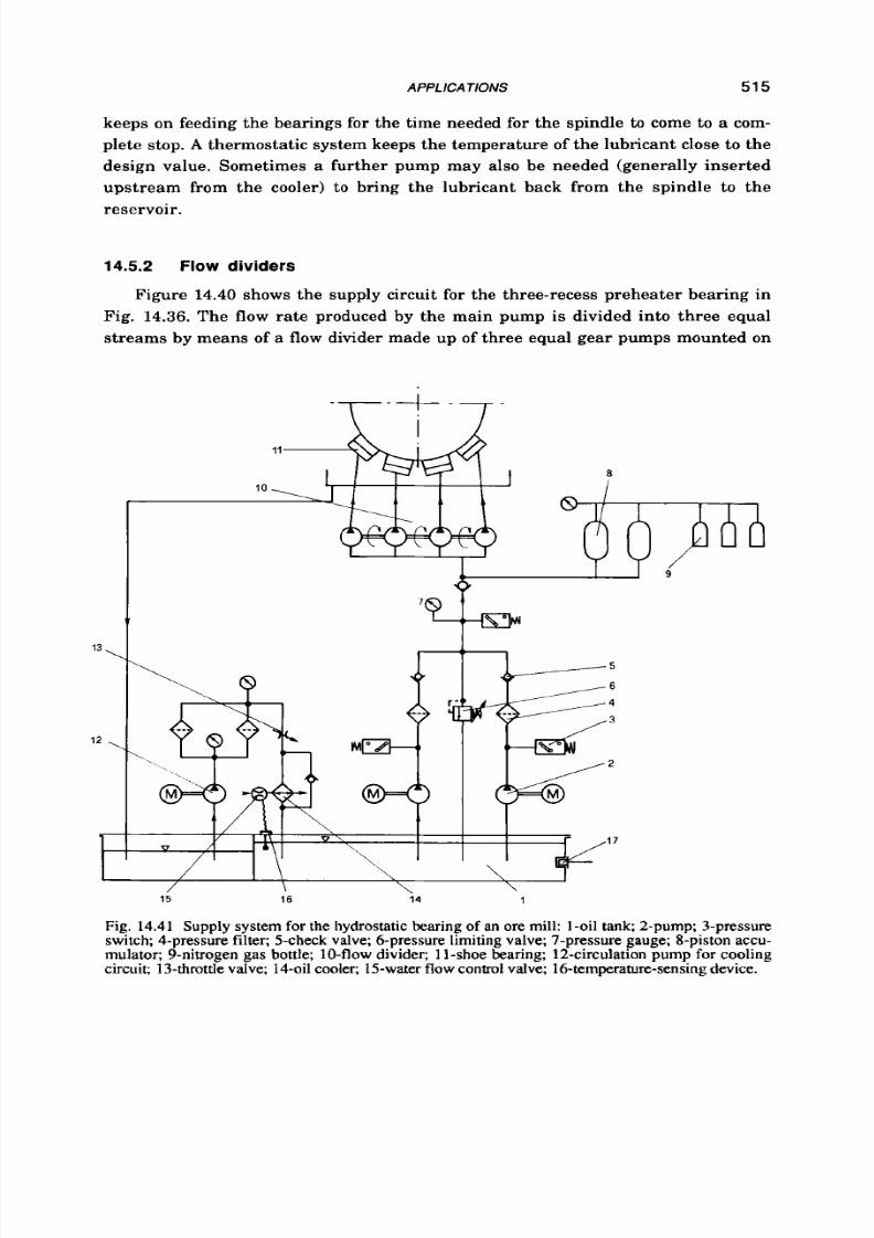
8/9/2019 Hydrostatic Lubrication 1992
http://slidepdf.com/reader/full/hydrostatic-lubrication-1992 532/558
APPLICA TlONS
515
keeps on feeding the bearings for the time needed for the spindle to come to a com-
plete stop.
A
thermostatic system keeps the temperature of the lubricant close to the
design value. Sometimes a further pump may also be needed (generally inserted
upstream from the cooler)
t o
bring the lubricant back from the spindle to the
reservoir.
14.5.2
Flow div iders
Figure 14.40 shows the supply circuit for the three-recess preheater bearing in
Fig. 14.36.The flow rate produced by the main pump is divided into three equal
streams by means of a flow divider made up of three equal gear pumps mounted on
\
3
8
1
1 9
17
5
6
4
3
2
15 16 14 1
Fig. 14.41 Supply system for the hydrostatic bearing
of
an ore mill: 1-oil tank; 2-pump; 3-pressure
switch; 4-pressure filter; 5-check valve; 6-pressure limiting valve; 7-pressure gauge; 8-piston accu-
mulator; 9-nitrogen ga s bottle; 10-flow divider; 1 1-shoe bearing; 12-circulation pum p
for
cooling
circuit 13-throttle valve; 14-oil cooler; 15-water flow control valve; 16-temperature-sensing device.

8/9/2019 Hydrostatic Lubrication 1992
http://slidepdf.com/reader/full/hydrostatic-lubrication-1992 533/558
51
6 HYDROSTATIC LUB RICATlON
a common shaft. To ensure continuous operation a second pump is ready to be
started up automatically when supply pressure drops below
a
safe value. A further
spare pump is available for replacement, to permit maintenance operations. In the
case
of
an electric mains failure a diesel generator can provide power for the motors
of the pumps. The last emergency device is a set of oil accumulators which can
supply lubricant to the bearings for a short time.
The hydraulic circuit for the bearing arrangement in Fig. 14.25
is
shown in Fig.
14.41. The flow rate produced by the main pump is divided into four equal streams
by means of a flow divider. To ensure continuous operation a second pump
is
ready
to be started up automatically in case of failure of the other one and
a
set of piston
accumulators (driven by pressurized nitrogen bottles) can feed oil to the bearings for
a certain time in case
of
power failure, allowing the runner
to
stop without damag-
ing the bearings.
14.5.3 Mult ip le pumps
The constant-flow supply circuit
of
the guideway presented in Fig. 14.22.b is
shown in Fig. 14.42. The pre-feeding pump (1)delivers lubricant at
a
pressure of 25
bar to two multiple pumps (2). Each pump can feed ten recesses independently,
each with a
0.33
m3/s flow rate, a t a pressure
of
40 bar.
Fig.
14.42 Supply system, with multiple pumps,
of
a hydrostatic slide.

8/9/2019 Hydrostatic Lubrication 1992
http://slidepdf.com/reader/full/hydrostatic-lubrication-1992 534/558
A PPLlCATlONS 517
Figure 14.43 shows the supply circuit of the pad arrangement in Fig. 14.33.
Each pad is directly fed at a constant flow rate; that is, a set of five multiple pumps
is used and each pump delivers
four
equal streams which
are
supplied to four pads
situated a t
90
degrees from each other. Thanks to the layout mentioned, emergency
operation of bearing system is
possible even if
a
pump fails.
Fig. 14.43 Supply system
for
the bearing system of a large-beam antenna: M-motor; P-multiple
pump; 1-20pads.
REFERENCES
14.1
14.2
14.3
14.4
14.6
14.6
14.7
Die Arbeitsspindel und Hire Lagerung
-
Herzstuck Leistungsfahiger Werk-
zeugmaschinen; FAG publ. 02-113 A (1985); 8pp.
Hallstedt
G.;
tandardized Hydrostatic Bearing Units;Instn. Mech. Engrs.,
C48
(1971),420-430.
Lewinschal L.; Contributo dei Cuscinetti Zdrostatici allXumento di Produt-
tivitb delle Rettificatrici;La Rivista dei Cuscinetti/SKF, 196(19781, 4-27.
FAG Spindeleinheiten fur das Bohren-Drehen-Frasen; FAG publ. 02-1OW3
DA (1985); 2pp.
Hydrostatic Shoe Bearing Arrangements;SKF Publication 3873 E (19881, 8
PP.
Bildtsh C., Htillnor G.; Problema Risolto con 1'Adozione di Pattini Idrosta-
tici;
La
Rivista
dei CuscinettYSKF,
181
(1974),18-20.
Polseck M., avra
Z.;
The influence of different types of guideways on the
static and dynamic behaviour of feed drives;Proc. 8th Int. MTDR Conf. (19671,
pt. 2,
p.
1127-1138.

8/9/2019 Hydrostatic Lubrication 1992
http://slidepdf.com/reader/full/hydrostatic-lubrication-1992 535/558
518
HYDRCSTATIC LUBRICA
TlON
14.8
Catalog B1025E;Nachi Corp., Japan,
1984; 4
p.
14.9
Weck M.; Handbook of Machine Tools, Volume 2 (Construction and Mathe-
matical Analysis);
J.
Wiley & Sons,
1980; 296
pp.
14.10
Rohs H. G.;
Die Hydostatische Bewegungspaarung im Werkzeugmaschinen-
bau;Konstrudion,
22 (1970); 321-329.
14.11
Andreolli C.; Eliminazione dell'Attrito e dei Giochi nelle Macchine Utensili;
Controlli NumericiIMacchine a CN/Robot Industriali, anno XI1 (19791, n. 7,
14.12
Appoggetti P.; Perfezionamento negli Accoppiamenti Vite-Cremagliera a
Sostentamento Zdrostatico;Patent IT
51829 N69;
Bollettino Tecnico RTM n.
9,
14.13
Umbach R., Haferkorn W.; Some Examples and Problems in Zmplementa-
tion of Mwlern Design Features on Large Size Machine Tools;
10th
Int. MTDR
cod., Manchester,
1969;
paper
34; 30
pp.
14.14
Rototraversing Tables for Indexing, Milling and Turning; INNSE Publication
DMU/27 (1985),4
pp.
14.15
Weck M.; Handbook of Machine Tools, Volume
3
(Automation and Controls);
J . Wiley & Sons,
1980; 451
pp.
14.16
Rippel T., Hunt J.
B.;
Design and Operational Experience of 102-Znch Diame-
ter Hydrostatic Journal Bearings for Large Size Tumbling Mills; Instn.
Mech. Engrs.,
C16 (1971), 76-100.
14.17
Arsenius H. C., Goran R.; The Design and Operational Experience
of
a Self-
Adjusting Hydrostatic Shoe Bearing for Large Size Runners;
Instn. Mech.
p.
32-45.
1969;
p.
47-51.
EWS.,
C303 (19731,361-367.
14.18
Supporti idrostatici FAG;FAG Publication
44109
IB
(19711, 8
pp.
14.19
Andreolli C.; Guida Circolare Idrostatica Assiale per Tavola Portapezzo
Rotante;Patent IT
2353CA, 1975; 15
pp.
14.20
Andreolli C.; Sopporto Zdrostatico per 1'Asse Azimutale del 3.5 m New Tech-
nology Telescope (NTT) dell %SO; Convegno AIM-AMME (Tribologia-Attrito,
Usura e Lubrificazione), Sorrento, 1987;p. 421-430.
14.21
Giordano M., Boudet M.;
Thermohydrodynamic Flow of a Piezoviscous Fluid
Between Two Parallel Discs;J. Mech. Eng.,
1980.
14.22
F r h e J ., Nicolas D., Deguerce B., Berthe D., Godet M.; Lubrification Hydro-
dynamique; Edition Eyrolles, Paris,
1990; 488
pp.
14.23
Martin
F.
J.; Prove Funzionali e di Qualificazione nello Sviluppo dei Cusci-
netti Volventi;
La Rivista dei CuscinettiBKF,
224
(1986),28-36.
8/9/2019 Hydrostatic Lubrication 1992
http://slidepdf.com/reader/full/hydrostatic-lubrication-1992 536/558
APPENDICES
A . l SELF-REGULATED PAIRS AND SYSTEMS
The principle of self-regulating flow, applied to circular bearings and screws
and nuts, can also be applied
t o
pads of infinite length. See the pair of pads shown in
Fig. Al.l.a, clearly
similar,
from the functional point of view, to the bearing in Fig.
7.25.
The formulae and the corresponding diagrams are also quite similar (see ref.
7.5).
Naturally the pad of finite length needs lateral seals. Consider, for example,
those shown in Fig. Al.l.b, made of two shaped plates 3, in the peripheral grooves of
which internal (static)
3.1
and external (dynamic)3.2 seals are housed. The former
are elastomeric seals while the latter are made of a material with a very low friction
coefficient (PTFE), which can be lowered even further by allowing small side
leakage.
A fur ther development
of
the principle of self-regulation
is
its application to
mutually orthogonal pairs of opposed pads of infinite length (ref. 2.23). Figure A1.2
schematically shows that application.
A
purely vertical load has almost no effect on
the gaps of the horizontal pairs while
it
makes the vertical ones bearing
it
work
as
self-regulating. Similarly a purely horizontal load makes the horizontal pairs work
as self-regulating bearings. The simultaneous presence of a vertical load and a
horizontal one, each supported by the corresponding self-regulating pair, involves
the self-regulation of
total
flow Q, which
is
subdivided into two equal partial flows
Q12 which are again subdivided into two equal partial flows Ql4. For the formulae
and the relevant diagrams the reader is referred to ref. 2.23. The hydrostatic system
in Fig. A1.2 which has the same advantages
as
self-regulated pads, in particular
very high stiffness, is directly applied in hydrostatic slideways. Obviously, lateral
seals of the type shown in Fig. Al.1.b will be necessary.

8/9/2019 Hydrostatic Lubrication 1992
http://slidepdf.com/reader/full/hydrostatic-lubrication-1992 537/558
520
HYDROSTATIC LUBRICAT I m
- a -
I?
-
b -
Fig.
A l . l
Self-regulating opposed-pad hydrostatic bearing: a- theoretical bearing; b- actual bear-
ing with side
seals.
A
further application of the principle of self-regulation is that of a system made
up of a self-regulating screw and nut in series with the above-mentioned slideway.
Self-regulating circular bearings, screws and nuts, pads and mutually orthog-
onal pairs, can be supplied
at
constant pressure a s well as with constant flow rate.
A s
for circular bearings, the matter has been discussed in section 7.4.2 and in
ref.
A l . 1 ,
where it is pointed out tha t the efficiency of the self-regulating bearing is
comparable to that
of
a conventional one fed through two flow-control valves. For
equal flow rate and pumping power in particular, the load capacity of the self-regu-
lating bearing
is
generally higher than tha t of the conventional bearing, especially
if the latte r is fed through capillaries
o r
orifices.
What has been said above also holds good for self-regulating screws and nuts,
compared in ref. A1.2 with the conventional ones fed through two flow-control

8/9/2019 Hydrostatic Lubrication 1992
http://slidepdf.com/reader/full/hydrostatic-lubrication-1992 538/558
APPENDICES
521
Fig.
A l . 2
System of self-regulating opposed-pad hydrostatic bearings.
valves. What has been said abovealso holds good for self-regulating pads, compared
in ref. A1.3 with conventional pads fed through capillarieso r orifices.
Finally for systems made up of mutually orthogonal pairs of opposed pads,it is
pointed out, ref. A1.4, that the self-regulating system bears higher loads than the
conventional system with fixed compensators and the phenomenon
is more marked
as
the load increases. Again, a further application of self-regulation consists in a
screw and nut assembly in series with a slideway.
A.2
DYNAMICS
In Chapter 10 the dynamic behaviour of hydrostatic bearings has been studied,
using linear mathematical models and Laplace transform. For a bearing with a
circular recess (Fig. 5.11, directly supplied by a pump with constant flow Q, arry-
ing a static load W and subjected to an instantaneous overload LW, he non-linear
mathematical model yields the following equation (ref. A2.1)

8/9/2019 Hydrostatic Lubrication 1992
http://slidepdf.com/reader/full/hydrostatic-lubrication-1992 539/558
522 HYDROSTATIC LUBRICATION
(A2.1)
where h ' = h / h , ,h , being the film thickness under the final static load W+AF (which
may be due to gravity),
which can be considered
a
damping constant,
C s = 2 m ,
where M is the bearing
mass and
K,=9pr~(1-r'2)Qlh4,
ts stiffness; C, can then be considered to be the criti-
cal damping;
is another damping constant;
is the fluid stiffness, K, the apparent bulk modulus
c
the fluid in the supply tube and in the recess.
the fluid and
\
the volume of
The initial conditions in Eqn
A2.1,
at the time t ' =O , are the following
where ho is the film thickness under load W and t ' = t / t s ,with
t s = 2 n m s
period).
Film and recess pressures are
(A2.2)
respectively, where p ' = p / p s ,p; =p , lp , and p s is the recess pressure under load
W + A F .
In Fig.
A2.1, A2.2
and
A2.3
the variations of film thickness
h'
and of recess and
film pressures p i and p ' , versus time are plotted. The former are determined by
solving Eqn
A2.1
numerically, the lat ter by introducing the values
of
h',
h'
and
x '
obtained from Eqn A2.1 in Eqns A2.2. The results concern the cases defined in Table
A2.1.

8/9/2019 Hydrostatic Lubrication 1992
http://slidepdf.com/reader/full/hydrostatic-lubrication-1992 540/558
APPENDiCES
case
1
2
3
523
'2 r' p . 1 0 2 W AF h , .104 K , . I o - ~ K ~ . I o - ~ ~ I K ,
m Ns/m2 N N
m
N/m N/m
0.05
0.9 5.4
1000
430 0.9
48 77
1.6
0.05
0.9
5.4
500
1500 0.95
63
77
1 .2
0.025 0.875 5.4 1000
430 0.9
48 7.7
0.16
In the first case the bearing is stable (Fig. A2.l.a).
After
a few oscillations it
stops in the equilibrium position
h'= l .
Figure A2.1.b shows
an
over-pressure in the
inner part of the bearing clearance followed, however, by a
small depression in the
outer part with possible cavitation and development of air bubbles.
- a - - b -
Fig. A2.1 Stable pad: a- oscillation of film thickness h' and recess pressure $; b- recess pressure
p i
and film pressure p'. Start of cavitation in the film.
In the second case the bearing is the same but the initial load is lower while the
instantaneous over-load is higher. Anyhow the bearing is still stable (Fig. A2.2.a)
but the initial oscillations are larger and the bearing comes to a stop after a greater
number of oscillations (interrupted in the diagram). Figure A2.2.b shows a consid-
erable over-pressure followed by a remarkable dangerous depression. Of course, in
such a case, cavitation must be considered in the numerical solution otherwise it
yields meaningless results.
In the third case the bearing
is
smaller but with the same loads
as
in the
first
case. It is unstable (Fig. A2.3): film oscillations ("relaxation oscillations", charac-
teristic of a self-exciting system (ref. A2.2) with positive damping) settle a t very high
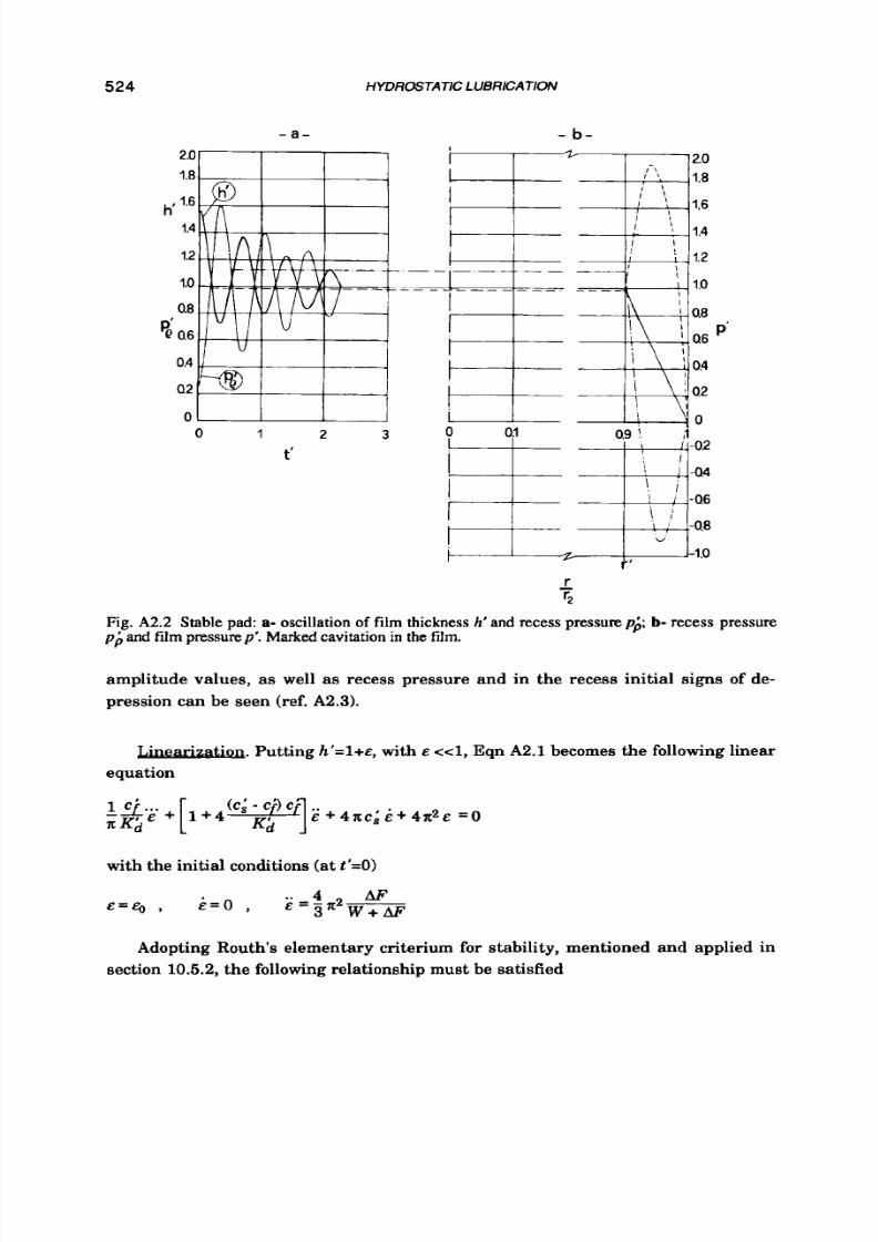
8/9/2019 Hydrostatic Lubrication 1992
http://slidepdf.com/reader/full/hydrostatic-lubrication-1992 541/558
524
--
OA
I
I
HYDROSTATIC LUBRICATION
n
~ 2.0
P\, 1.8
I
:
I ,
I (
5 -1.6
: 1.4
I 1
I
I 1
I i
12
I
I ~ 1.0
- .
--
- -
I
0.8
\ I 06 P'
T
i \
I
0.4
1
8
;
0.2
I
0
I
1 -02
i I
0.9 1
,I
-a4
' ;
\, ;
; ..-0.8
' - 4 6
"
"
-1.0
i'
amplitude values, as well as recess pressure and in the recess initial signs of de-
pression can be seen (ref. A2.3).
-
Putting h'=l+&,with E <el, qn A2.1 becomes the following linear
equation
with the initial conditions
(at t '=O)
.. 4 AF
E = Q
, E = O
, E
= p 2 -
Adopting Routh's elementary criterium for stability, mentioned
and
applied in
section 10.5.2, the following relationship must be satisfied
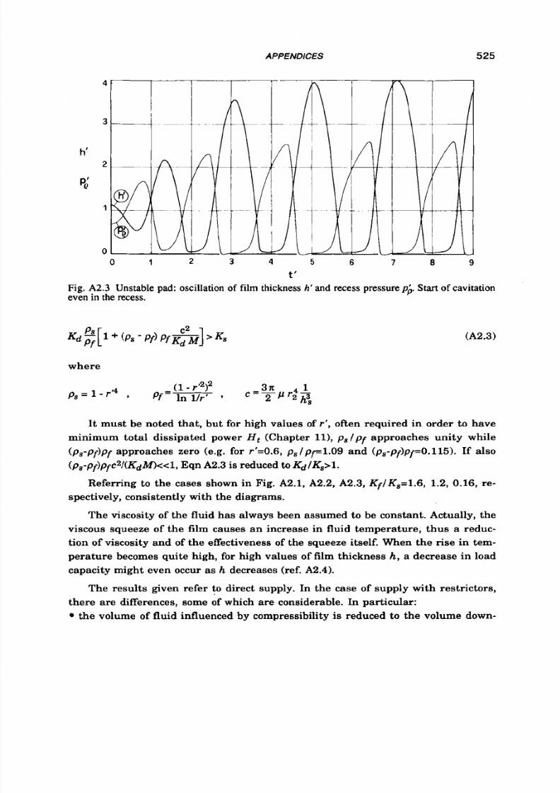
8/9/2019 Hydrostatic Lubrication 1992
http://slidepdf.com/reader/full/hydrostatic-lubrication-1992 542/558
APPENDICES
525
4
3
h’
2
pd
1
0
0
1
2 3 4 5
6 7
a 9
t‘
Fig. A2.3 Unstable pad: oscillation of film thickness h‘ and recess pressure p i . Start of cavitation
even in the recess.
(A2.3)
where
It must be noted that, but for high values of r’, often required in order
to
have
minimum total dissipated power H , (Chapter 111, p s l p f approaches unity while
(p,-pf)pf
approaches zero (e.g. for
r’=0.6,ps
/pf=1.09and (ps-pf)pf=0.115).f a l s o
(ps-pf)pfc2/(KdM<<1,qn A2.3
is
reduced
to
Kd/Ks>l.
spectively, consistently with the diagrams.
Referring to the cases shown in Fig. A2.1, A2.2, A2.3, KflKs=l .6 ,1.2, 0.16, re-
The viscosity of the fluid has always been assumed to be constant. Actually, the
viscous squeeze of the film causes an increase in fluid temperature, thus
a
reduc-
tion of viscosity and of the effectiveness of the squeeze itself. When the rise in tem-
perature becomes quite high, for high values of film thickness h, a decrease i n load
capacity might even occur as
h decreases (ref. A2.4).
The results given refer
t o
direct supply. In the case of supply with restrictors,
there are differences, some of which
are
considerable.
In
particular:
the volume of fluid influenced by compressibility
is
reduced to the volume down-

8/9/2019 Hydrostatic Lubrication 1992
http://slidepdf.com/reader/full/hydrostatic-lubrication-1992 543/558
526 HYDROSTATIC LUBRICATION
stream from the restrictor;
. f the restrictor is rigid, it works as a damper. This does not mean that compen-
sated supply is better than direct supply from this point of view, because, on the
contrary, the lat ter shows higher damping, as can be seen in Chapter
10;
if the restrictor is variable, it may produce a negative effect because the number of
degrees of freedom increases.
As
regards degrees of freedom, a bearing, and a hydrostatic system in general,
is part of a bigger system: a machine made up of various elements (each with its
own stiffness and internal damping), therefore with various degrees of freedom.
It should also be noted that hydrostatic systems, because of the fact that their
films work a s vibration attenuators (ref. A2.5),may be preferred to other low friction
systems in those machines in which forced vibrations are expected, especially if
resonance is possible, and with several degrees of freedom. In this connection, it
must be pointed out that very stiff films are not always convenient because they
would behave in practice as stiff elements with no damping properties.
A.3 THERM AL EXCHANGE
A.3.1
Resistances
In the case of laminar flow with forced convection in a tube
of
diameter
d
and
length 1, that is for Red =V d/ v<2000, the Nusselt number is
where Pr=pccll is the Prandtl number and
I
fluid thermal conductivity. It s thermal
unit conductance is
(A3 .1)
For
fluids with high P r , such
as
lubricating oils, in long tubes, with good approxi-
mation
Nud=3.66,
thus
'yc=3.66(Ild).
The lubricant thermal resistance in the tube is
where A is the wet surface. Considering the recess as a rectangular tube, i ts equiv-
alent diameter is

8/9/2019 Hydrostatic Lubrication 1992
http://slidepdf.com/reader/full/hydrostatic-lubrication-1992 544/558
APPENDICES
for L>>h, (in the examples given L=40h,.).So R 1 , becomes
527
Its value may be increased without causing any problem (almost doubled). R 1 , can
be determined in the same way.
For turbulent flow, that is for
Re&6000,
and the values of NUd can be much higher than those relevant to the laminar flow.
In transient conditions, that
is
for
2000dZedC6000,
the evaluation of
NUd
is very
difficult.
A.3.2 Coeff icients
A.3 .2.1 coefficient
ac
i)
Forced convection on an infinite plate of width B with fluid lapping a t one face,
a t speed V , far from the face.
N U H
=
0 . 6 6 4 Re ~ l"PrIf3
and since
Pr=0.72
for air
N U H
=
0.595
ReBlI2
This formula is true for laminar
that is for
Rt?B=V,B/ ~ 4 5 . 1 0
values, not easily achievable, flow becomes turbulent, and
N U H
=
0.036 (ReBo.8 23,2 00)Pru3
and for P-0.72
NUH = 0 . 0 3 2 R e ~ ~ . ~748
( A 3 . 2 )
for higher
Forced convection on an infinite plate of width
B ,
for
R e ~ C 5 . 1 0 5 ,
ith flow per-
pendicular to one face. The relationship
NuBa = o . 1 5 R f ? ~ ~ ~ ~ ( A 3 .3 )
can be used with a good approximation.
Trail of an infinite plate of width
B ,
for
R e ~ C 5 . 1 0 ~ .

8/9/2019 Hydrostatic Lubrication 1992
http://slidepdf.com/reader/full/hydrostatic-lubrication-1992 545/558
528
HYDROSTATIC LUBRICATION
(A3.4)
With equations
A3.4, A3.2
and
A3.3,
the conductance
a,
of a prismatic structure
(slideway) of infinite length can be roughly evaluated. For example, for
B = l
m and
thickness
H=0.2
m, and for
V,=50 d s ,
with
v=1.6.10-5
m2ls for air, it is
R e ~ , = 1 7 6 8 ,
Re g = 7 N . 6 ,Re g p 2 1 3 7 0 . ThereforeN U ~ ,= 2 6 5. 2, u ~ = 4 7 0 . 4 , u ~ , = 4 2 7 . 5 ,o % ~ , = 7 . 1 6
J/ms2s°C, a c B= 6 3 . 5 J/ms2s0C, acB,=115.4 J/ms% C and the average value is
a,=(
c g a + 2 a c ~ +& , ) /4=62.5 /ms2s°C.
ii) Natural convection around a square plate of side
B
and thickness
H
much
smaller than B , with flow perpendicular
t o
one face:
N U B= 0.45 (G rg pr)'I4
where
Grg is
the Grashof number which in natural convection replaces
R e ,
where d e q = 2 [ B H / ( B + H ) ] ,? is the coefficient of volume expansion,
T,
surface tem-
perature and
T,
the air temperature far from the surface.
For
Pr=0.72,
N U B
=
0.414 (Gr#4
This formula is true for laminar flow, that is for G r ~ < S . l o ~ ;or higher values of
Grg, that is for turbulent flow,
NUB=
0.083
(Grg
Pt')y3
The corresponding values of spy, obtained from Eqn A3.1, substituting
d
with deq,
are small anyhow. For example, for
B=0.15
m,
H=0.015
m,
T,=5OoC, Tm=2OoC,
since
(gp)/v2=108
/m3 C for air,
G r ~ = 6 . 1 . 1 0 ~ ,
hus
N U B=6.5,
and since
k 0 . 0 2 7
J1ms C for
air , from Eqn
A3.1 in which d
is
replaced by deq,we have a,=6.4 J/ms2s°C.
by (L+B)/2.In the case of a disk of diameterD, is substituted by 0.9D.
In the case of a rectangular plate of width B and length L ,
B
may be substituted
iii) Horizontal rotating disk of diameterD, ith flow perpendicular to a face.
w D 2
v2
NuD
=
0.18
7)
8/9/2019 Hydrostatic Lubrication 1992
http://slidepdf.com/reader/full/hydrostatic-lubrication-1992 546/558
APPENDICES
529
The boundary layer is laminar if R e ~ < 5 . 1 0 6 ;or higher values
where D , is smaller than D and decreases with w , and flow is laminar from 0 to
D J 2 and turbulent from D J 2 to 012 . For example, for w=500 s-1, D p O . 1 2 7 m. For
D=0.2
m flow
is
laminar from
0
to
0.0635
m and then it becomes turbulent. Therefore
N u ~ = 3 . 5 . 1 0 ~
nd
q = 4 7
Jlms2sOC.
In
ref. 5.15 the cooling of the lubricant is due to the high speed(-628
rads)
and
the large diameter of the rotating disk ( D = 0 . 3 m) and mostly to the “ducted fan”
effect.
iv) Horizontal rotating cylinder of diameter
D,
ith flow perpendicular to its axis.
For rotational speed
w
lower than the critical value, that is for R e ~ < 2 . 5 . 1 0 ~ ,ee the
following case of the motionless cylinder; for higher values, the flow becomes turbu-
lent and
This formula can be used for journal bearings.
Natural convection around
a
horizontal cylinder of diameter D , with flow per-
pendicular to its axis.
and for
P r 4 . 7 2
This formula
is
true for laminar flow, that
is
for
G r ~ < 5 . 1 @ ;
or higher values, that
is for turbulent flow,
and forPr=0.72
For
example, for
D=O.OOl
m, T,=50°C, T,=20°C, we have
G r p 3 . 1 0 3 ,
thus
N u ~ = 3 . 6
nd
q = 9 . 6 2
J/m2soC. With the simplified formula
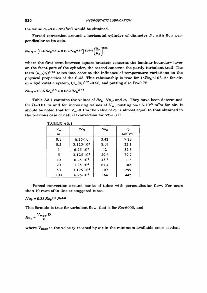
8/9/2019 Hydrostatic Lubrication 1992
http://slidepdf.com/reader/full/hydrostatic-lubrication-1992 547/558
530 HYDROSTATIC LUBRlCATfON
the value q=8.5J/mspsOCwould be obtained.
Forced convection around a horizontal cylinder of diameter D, with flow per-
pendicular to its axis.
where the first term between square brackets concerns the laminar boundary layer
on the front part of the cylinder, the second concerns the partly turbulent trail. The
term
(pU,/p,)O.25
akes into account the influence of temperature variations on the
physical properties of the fluid. This relationship is true for l I R e ~ 1 l O ~ .s for air,
in a hydrostatic system, (p,/&0.25=0.98, and putting also Pr=0.72
Table A3.1 contains the values of ReD, NuD and ac.They have been determined
for D=O.Ol
m
and for increasing values of V, , putting ~ = 1 . 6 . 1 0 - ~2/s for air.
It
should be noted that for
V,=O.l
m the value of q s almost equal to that obtained in
the previous case of natural convection for AT=30°C.
‘ A B L E A 3
v,
m
0.1
0.5
1
5
10
20
50
100
1
Re,
6.25 .10
3.125.102
6.25 .102
3 . 1 2 5 1 0 ’
6 .25 .103
1.25.104
3.125 .104
6 . 25 .
1
04
3.42
8.19
12
29.6
43.3
67 .4
109
164
a,
J/m*s°C
9.23
22.1
32.3
79 .7
117
182
295
442
Forced convection around banks of tubes with perpendicular flow.
For
more
than 10 rows of in-line or staggered tubes,
Nub = 0.33Reb0.6Prv3
This formula is true for turbulent flow, that is for Re>6000, and
where Vm, , is the velocity reached by air in the minimum available cross-section.
8/9/2019 Hydrostatic Lubrication 1992
http://slidepdf.com/reader/full/hydrostatic-lubrication-1992 548/558
APPENDICES
531
For laminar flow (Reb<200) and also for transient flow (200dEeb<6000) the
relationship
NUb
= J
Reb Pru3
is true. This formula is complicated because
j ,
which is Colburn's dimensionless
factor, is a function of R e , of the number of rows of the tubes and of their
arrangement.
A
grid upstream from the bank
of
tubes makes turbulence possible even at low
Reynolds numbers. Barnes in the bank make the air move in a winding way, thus
increasing the actual surface
of
heat transfer.
A.3 .2.2 Coefficient
aj. Coefficient aj for air is:
where F11.2=o.7o 0 . 9 is the geometric form factor, 0=5.7 J/m2s°K is the Stefan-
Boltzman constant,
TI
nd
T2
are body and ambient temperatures, respectively. For
temperatures included in the hydrostatic range, aj=4.5 to 7 . 5 J/m2s°K, approxi-
mately. Such values must be added to ac in order to obtain the global unit conduc-
tance a.
What has been described above can be useful for the design of an air-oil heat
exchanger with the tube bank made of the hydrostatic system supply pipelines, bent
more times to a
U
shape. The approximate value of the coefficient of global heat
transfer for air-oil exchangers is
a=30
to
180
J/m2s°C.
For high lubricant temperature rise it may be advisable t o use water-oil heat
exchangers for which a=120 to 350 J/m2s°C approximately (ref. A3.1) . Water heat
exchangers, as well as air exchangers, can be placed in the return line; however,
the absence of water o r air leakage in the lubricant must be carefully checked.
Finally, when heat exchangers are placed in the supply line, a more effective
control of the temperature of the bearings may be obtained.
REFERENCES
A l . l
Bassani R.;
The Self-Regulated Hydrostatic Oppo sed-Pad Bearing in a Con-
stant Pressure System;
ASLE
Trans.,
25,
(1982) ,95-100.
A1.2 Bassani R., Piccigallo B.; Vite-Ma dreuite Zdrostatica Autoregolata Ali m enta -
ta a Pressione Costante; Tribologia e Lubrificazione, AMO XIV (1979) ,98-109.
8/9/2019 Hydrostatic Lubrication 1992
http://slidepdf.com/reader/full/hydrostatic-lubrication-1992 549/558
532
HYDROSTATlC LUBRlCATfON
A1.3 Bassani
R.;
Pattini Contrapposti Zdrostatici Autoregolati, Al im en tat i a Pres-
sione Costante; Oleodinamica-Pneumatca,24(19831, 8-25.
A1.4 Bassani
R.;
Sistema d i Pattini Zdrostatici Autoregolati, Alim en tat i a Pres-
swne Costante;
Scritti
per L. Lazzarino; Pacini Editore,
Pisa, 1986;
.
235-250.
A2.1 Bassani
R.;
Cuscinetti Zdrostatici di Spinta Sottoposti a Varia zioni Istantanee
del Carico;
2nd
AIMETA Congr., Napoli,
1974;
ol.
3,
p.
225-236.
A2.2
Nayfeh A.
H.,
Mook D. T.;
Non linear oscillation;
J.Wiley & Sons Inc.,
1979;
704pp.
A2.3 Hell H., Savci M.; Bynamische Eigenshaften Hydrostatischer Axiallager bei
Kleistmilglichem Gesamtleistungsaufwad;Konstruction, 27 (19751, 37-144.
A2.4 Pinkus
O.,
Wilcock D. J.; Thermal Effect in Fluid Film Bearing; Mech. Engi-
neering Publ. Ltd,
1980;
.
3-23.
A2.5
Wilcock D. F.,Bevier W. E.; Externally Pressurized Bearings.
-
Vibrat ion
Attenuators; ASME
Trans.,
J.
of
Lubrication Technology,
90(19681,614-617.
A3.1
Wilcock D.
F.,
Booser E.
R.; Lubrication Technique for Journal Bearings;
Machine Design, June 25,1987; 84-89.
8/9/2019 Hydrostatic Lubrication 1992
http://slidepdf.com/reader/full/hydrostatic-lubrication-1992 550/558
Author index
For each author this index shows the relevant reference numbers, as well as
the pages on which each reference is cited. For example
Fuller
D. D.
1.5-
4, 141, 143
The reference is the fifth item in the reference list of chapter
1
and is cited on pages
4,141
nd
143.
Andreolli C.
14.11- 495
14.19- 5@?,510
14.20-
509
Anwar I.
Aoyama T.
AppoggettiP.
Arsenius H.C.
Arsenius T.
Artiles A.
Barrett
L.
C.
10.7-
322,339
Bassani R.
2.10-
23
2.19-
28
2.23- 30,519
4.11- 81,101
5.1-
94
5.2-
%, 98
5.4- 98, loo
5.5- 98,100
5.9-
1 M
5.10-
105,107
5.14-
107,111,447
5.15-
107, aS,
447,529
5.16-
111
5.18- l22
5.31- 135
8.2- 237
8.29- 261,263
14.12- 496
14.17- 504,505
2.2-
17,486,487,512,613
8.15-
245
Bassani R. (continued)
5.32- 135
5.42- 145
5.43-
146,227
7.5- 221,223,619
7.6- 223
7.7-
29,339
7.8- a.2
13.5- 470
13.6- 470
13.9-
478
13.10- 480
13.11-
480
Al.l- 520
A1.2- 520
A1.3- 521
A1.4-
521
A2.1- 521
14.22- 511
Berthe D.
Bettini B.
8.8- 239
Bevier W. .
A2.5-
526
Bil dts h C.
14.6- 491,492
Bird R. B.
12.1- 447
Booser
E. R.
3.4-
40,42
10.1- 301,304
A3.1- 531
Bottcher
R.
BoudetM.
Boyd J.
14.21- 511
3.2-
37
8.5- 238
Brzeski L.
2.17-
27
Bucciarelli A.
3.9- 47
Cameron A.
4.4- 69,81
Casely A. L.
2.8- 22,169
Castelli V.
5.28- 135
Chang T.
S.
5.37-
142
Chen B.
Chen C. R.
Chen K. N.
Chen
N.
N.
S.
8.25- 2-54
5.36- 142
10.4- 302,320,358
8.13- 245
8.14- 245
Chen Y.S.
Chong F. S.
10.14- 356
9.2-
292,233,296
10.15-
356
8.2- 237
Colsher R.

8/9/2019 Hydrostatic Lubrication 1992
http://slidepdf.com/reader/full/hydrostatic-lubrication-1992 551/558
HYDROSTATIC LUBRICATION
34
Cowley A.
Culla C.
8.6-
238
5.32- 135
13.10-
480
13.11-
480
Czichos H.
Davies P. B.
13.1- 467
2.15- 26,470
8.7- 239
8.11-
240,242,244,354,355
13.7- 472
De Gast
J.
G. C.
2.11-
23
De Shepper M.
10.13- 356
Decker 0.
7.10-
233
7.9- 233
Deguerce
B.
14.22- 511
Dorinson A.
Dowson
D.
3.1- 36,37
2.14-
26
5.6-
lm,
104,110
5.21- 128,132
Dumbrawa M. A.
8.17-
W 50,254,419
8.18-
254,288
Effenberger W.
El Hefnawy
N.
8.20- 250
El Kayar A.
9.3-
292
El
Sayed
H.
R.
5.41- 144
El Sherbiny M.
El-Efnawy
N.
El-Sherbiny
M.
Ernst
P.
Et t les
C .
H. M.
4.6- 74
Fowle
T.I.
3.7- 44
Fr6ne
J.
14.22- 511
Fuller D. D.
Ga ne sa n
N.
10.1-
301,304
8.20- 250
4.8- 74
4.8- 74
7.1-
218,495,496
1.5- 4,141, 43
5.17-
l20,125
5.20- 128
8.30- 262,268
8.32-
262
10.5-
307
Geary
P.
J.
2.20-
28
Ghai R.
C.
8.3-
238
8.9- 240
Ghigliazza R.
Ghosh M.
K.
11.2- 419
10.10- 354
10.11- 354
10.17- 358,360
Giordano M.
14.21- 511
Girard L. D.
1.1- 4,35
Godet M.
14.22- 511
Goldstein S. D.
Goran R.
Haferkorn
W.
Hallnor G.
Hal lstedt G.
14.2- 485,487
Hegazy A.
A.
9.3- 292
Hell H.
A2.3-
524
Heller
S.
5.35-
142
Hessey
M. .
8.33- 264
I i i rai A.
Hirs G. G.
Ho
Y.
S.
8.13- 245
Hooke C. .
2.12-
25
8.1-
237
8.26- 255
4.1-
54
14.17- 504,505
14.13-
496, 98
14.6- 491,492
5.24- 132
2.13- 25,172
Hornung V. G.
Howarth R.
B.
4.5-
74,247
2.8- 22,169
13.4-
469
Hunt
J.
€3.
Ich ikawa A.
Ikeuchi K.
Inasaki
I.
14.16- 503,504
9.1-
290,292
2.24-
23
8.29-
261,263
10.9- 348,472
9.5-
298
Ives D.
Ives D. (continued)
J a i n
S.
C.
Kapur V.
K.
Karelitz
M. B.
Ka t suma t a S.
Kazimiersk i
2.
Kennedy J.
S.
Khalil
F.
9.6-
298
8.10- 240
5.12-
107,110
1.4- 4
8.2- 237
2.17-
27
5.13-
lW,
25
5.19-
125
5.25- 132,476
Khalil
M. F.
9.3- 292
Kha t a a n H . A.
5.41- 144
Kher A. K.
Kong
Y.
.
Koshal D.
8.6-
238
8.14-
245
8.19- 247,293
9.4- 293,294,296, 77
12.2-
451,456,461
Kreith F.
Kubo
M.
2.18- 27
7.4-
220
2.2- 17,486,487,511,513
4.9-
79
3.11- 52
10.12- 356
13.7- 472
Kundel K.
La ngha a r
H.
.
Lansdown A. R.
Leonard R.
Lewinschal L.
14.3-
487,488
Lewis G.
K.
5.23-
131
Lightfoot E . N.
12.1-447
Lingsrd
S.
8.14- 245
Loeb
A.
M.
5.34- 139,468
13.2- 468
Lombard J.
Lord Rayleigh
Ludema
K. C.
Lund J.
W.
5.40- 144
1.3-
4
3.1- 36,37
8.37-
282

8/9/2019 Hydrostatic Lubrication 1992
http://slidepdf.com/reader/full/hydrostatic-lubrication-1992 552/558
Lund J. W. (continued)
10.16-
356
Majumdar B.C.
10.11- 354
Makimoto Y.
2.18-
27
7.2-
218
Manea G.
Mart in
F. J.
Martin H. R.
Massa E.
Masuko M.
Ma t suba r a T.
8.16- 246
14.23- 512
3.5- 44,47,48
5.27- 135
10.2-
301
2.18-
27
7.2-
218
7.3- 220
7.4-
220
Mayer J. E.
2.9-
23
5.11- 107,110
McCloy D.
Meo F.
Merri t t
H. E.
Michelini
C.
Mizumoto H.
2.18- 27
7.2- 218
7.3-
220
7.4-
220
Mohsin M. E.
2.6- 21,29,167
Moisan
A.
Mook D. T.
Mori H.
3.5-
44,47,48
13.3- 469
2.7-
22,78,
o,
2,85
11.2- 419
5.40- 144
A2.2-
523
2.24- 23
5.24- 132
Morsi S. A.
2.5- W,65
10.6- 320
Morton P.
G.
Moshin M.
E.
9.6-
298
8.28- w6
10.6- 320
Mote C. D.
5.3-
98
Mueller-Gerbes
H.
7.1-
218,495.4s
N a k a h a r a T.
10.2- 301
AUTHOR
INDEX
Nayfeh A. H.
A2.2-
523
Neale J. M.
3.10-
50
Newton M.
J.
Nicolas D.
O'Connor J.
ODonoghue J. P.
13.4-
469
14.22- 511
3.2-
37
2.12-
25
4.6- 74
5.23- 131
5.26-
I 3 3
8.1- 2-37
8.26-
255
8.31- 2 M
8.33-
264
8.35-
279
8.36-
282
Ogate K
10.8- 324
o g i s o s.
Ohsumi
T.
Oka mur a S.
2.18- 27
Okasaki
S.
7.3- 220
Opitz H.
1.7- 4
2.3-
19,173,376
10.1- 301,304
8.27- 255
2.24- 23
Piccigallo B.
5.42-
145
5.43- 146,227
7.7- 229,339
A1.2- 5 W
Pinkus
0.
4.2- 54,68,81
A2.4- 525
PolsEeck M.
14.7- 492,496
Prabhu
T.
.
5.20-
128
8.30- 262,268
5.17- 120,125
8.32- 262
10.5- 307
Radkiewicz Cz.M.
Ragab H.
Raimondi A.
A.
Raznyevich
K
Recchia L.
5.13- 107,125
5.22-
l28,131,132
8.5-
2-38
3.8-
46,50
7.8- 232
535
Reddi M. M.
Rippel H. C.
5.29- 135
1.6- 4
5.33- 139
7.11-
233
13.2- 468
Rippel T.
Rohs
H.
G.
Rowe W. B.
14.16- 503,504
14.10- 500,503
1.9-
l0,89
8.1- 237
8.12- 241,244,353,355
8.19- 247,293
8.24-
253
8.26- 255
8.34- 276,277,278
8.35-
279
8.36- B2
9.2- 292,293,296
9.4-
293,294,296,377
9.5- 298
9.6- 298
10.12- 356
10.15-
356
Royle J. K
2.8- 22,169
Rumbarger J.
H.
5.39- 144
Sa f a r Z. S.
5.3-
%
Salem
E.
5.19- 125
5.25- 132,476
Salem E. A.
9.3- 292
Salem F.
4.8-
74
8.20- 250
Sa sa k i T.
Sato
Y.
Savci M.
Shapiro W.
5.24- 132
8.27- 2-55
A2.3-
524
5.28- 135
5.35- 142
7.9-
233
7.10- 233
8.4- 238
8.15-
245
Sha r ma S. C.
Shaw
H.
C.
Shen F. A
8.10- 240
2.9- 23
5.8- 106
8/9/2019 Hydrostatic Lubrication 1992
http://slidepdf.com/reader/full/hydrostatic-lubrication-1992 553/558
536
Shinkle
J.
N.
4.5- 74.247
Siddal
J.
N.
11.1-
385
SiebersG.
2.1-
17,490
Singh D.V.
8.3-
238
8.9- 240
Sinha P.
Sinhasan R.
5.13- 107,
I25
8.3-
238
8.9-
240
8.10-
240
So H.
5.36- 142
5.37- 142
5.7- 105
3.9- 47
1.8- 6 ,B , 115,133
so0
L.
s.
Speich H.
Stansfield F.
M.
SternlichtB.
Stewart W. E.
Stout K. J.
4.2- 54,68,81
12.1- 447
8.19- 247,293
8.24-
253
8.34-
276,277,278
Straccia P. F.
Streeter
V.
Szeri A. 2.
5.38- 142,239,261,264
4.10- 81
5.30- 135
HYDROSTATIC LUB RICATION
Taylor C. M.
2.14- 26
5.21- rzS,l32
6.11- 107,110
4.3-
54
4.7- 74
2.16- 27
Ting
L. L.
Tipei
N.
Tully
N .
Umbach
R.
Usuki
M.
Vavra 2.
Verma
K
Vermeulen
M.
14.13- 4%, 498
7.3- 220
14.7- 492,4%
5.12- 107,110
8.21- W0,Wl
10.13-
356
13.8- 474
Viswanath N. S.
10.17- 358,360
Vogelpohl G.
1.2-
4
Walowit J.
8.15- 245
Wang X.
Wearing R. S.
10.4- 302,320,358
8.35-
279
8.36- 282
Weck
M.
14.9- 4M
14.15- 502
Wertwijn
G.
5.39- 144
Weston W.
9.2- 292,293,296
9.6- 2M
Wiener H.
Wilcock
D.
F.
2.4- 20
10.3-
302
A2.5-
526
A3.1- 631
Wilcock D.
J.
A2.4-
625
Wills
J.
G.
3.3- 39
Wong G.S.K.
2.22-
30
Wu H. Y.
10.14-
356
Wylie
C.
R.
Xie P. L.
x u s.
xu
s.x.
Yang G.
P.
Yang
H.
H.
Yates S.
Yonetsu S.
Yoshimochi
S.
10.7-
322,339
10.14-
356
8.25- 254
9.2- 292,293,296
10.4- 302,320,358
10.4- 302,320,358
2.21- 28,279
8.29- 261,263
2.18- 27
8/9/2019 Hydrostatic Lubrication 1992
http://slidepdf.com/reader/full/hydrostatic-lubrication-1992 554/558
Subject
index
Bold page numbers indicate that the item
is
the main topic of a section.
Symbol
u->”
means “see”.
additives
50,51, 2
adiab atic flow 89,107,110,132,151,225,248,295
a i r en t ra inmen t 44, 45
air preheaters
511
ann u la r c lea rance 75-’33
a n n u l a r - r e c e s s p a d s 7,112 23,133,907,422-425
an tennas
5,508
appa rent bulk modulus -> equivalent b. m.
a t t i tude angle 292
Bernoulli equation 83
boring machines
6
boundary layer 79
bulk modulus 42,45,46,47
bulk modulus (equivalent) -> equivalent b. m.
capi l lar ies -> res t r ic tors ( laminar-f low r.)
cavitation 48,104,108,133,245,262,288
characteristic equation
322,323
c i rcu la r - recess pads
7,76-77,91-11,123,128,
305-307,4210
422,469,521
clearance -> f i lm th ickness
clearance ( radia l ) -> radia l c learance
compensated supply 16,17- 0,31,88,91,15372,
173,180- 86,192- 13,220- 21,312 20,
334-339,415-433
compensating devices -> res t r ic tors
compressibility
42,47, 26
conical bearings -> tapered bearings
conical pads
->
tapered pads
constant- f low supply
->
direct supply
cons tant- pressure supply -> compensated
constitutive equations
55
continuity equation 54-
58,59,61,64,77,81,107,
111
contraction coefficient 83
cooler 460
correction factors
96,98,99,100, 01,105, 11,118,
Couette flow
69,246,288
critical speed
73,74,356
supply
119,122,126,127
cryogenic fluids
245
cylindrical pa ds 9, 136- 41,151,233
dam ping coefficients (journal bear ings)
354,
356,360
damping factor 321,342,356
density 42-49,310
des ign
hybrid bearings 296- 97
mult i recess journ al bear ings 251-HI
mult i recess thr us t bear ings 263
opposed-pad bearings
213- 18
s ing le -p ad bea r ings 172- %
spherical bear ings
278
tapered bearings
269
Yates bearings 283-285
diaphragm bear ing s 27
direct supply
16,17,
O,
2,88,91,148 53,173,
177-
80,188
92,219, S-227,230,311-12,
333-334,988-381
discharge coefficient
84, 85
displacement (nondimens.) --> eccentricity
dynamic viscosity --> viscosity
dynamics 301- 61,472,474,521-
%
eccentr ic i ty
hybrid bearings
292
mult ipad journal bear ing s 233
mult i recess journal b ear ings 240, 242
opposed- pad bearing s
187
direct supply 192
flow divide rs 205
l am ina r - f low rest ri cto rs
195
screw-nut assemblies
direct supply 219
l am ina r - f low rest ri cto rs 220
s ing le -p ad bea r ings
89,302
Yates bearings 279
annu la r - recess pad 113,118,120
c i r c u l a r -recess pad
91,96,101,105,111
cylindrical pad
139
effective a rea 87
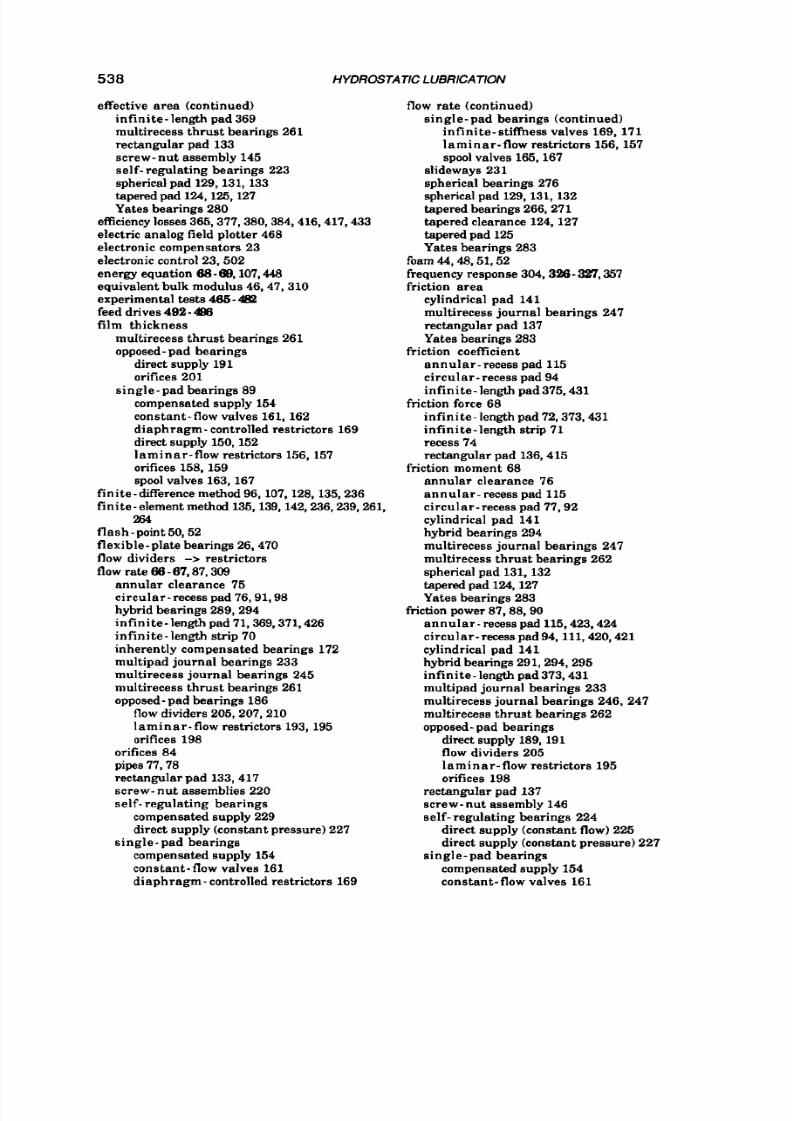
8/9/2019 Hydrostatic Lubrication 1992
http://slidepdf.com/reader/full/hydrostatic-lubrication-1992 555/558
538 HYDROSTATIC LUBRICATION
effective area (continued)
infinite-length pad 369
multirecess thrust bearings
261
rectangular pad 133
screw-nut assembly 145
self- regulating bearings
223
spherical pad 129,131,133
tapered pad 124,125,127
Yates bearings 280
efficiency losses365,377,380,384,416,417,433
electric analog field plotter 468
electronic compensators 23
electronic control 23,502
energy equation
CW-69,107,448
equivalent bulk modulus 46,47,310
experimental tests
485-
82
feed drives
492-433
film thickness
multirecess thrust bearings
261
opposed-pad bearings
direct supply 191
orifices 201
single-pad bearings 89
compensated supply 154
constant-flow valves 161,162
diaphragm- controlled restrictors 169
direct supply 150, 152
laminar-flow restrictors 156, 157
orifices158,159
spool valves 163,167
finite-differencemethod 96,107,128,135,236
finite-elementmethod 135,139,142,236,239,261,
flash-point50,52
flexible-plate bearings
26,470
flow dividers -> restrictors
flow rate 66
-
67,87.309
annular clearance 75
circular-recess pad 76,91,98
hybrid bearings 289,294
infinite-length pad 71,369,371,426
infinite-length strip 70
inherently compensated bearings 172
multipad journal bearings 233
multirecess journal bearings 245
multirecess thrust bearings
261
opposed-pad bearings 186
flow dividers 205,207,210
laminar-flow restrictors 193, 195
orifices 198
264
orifices 84
pipes 77,78
rectangular pad 133,417
screw- nut assemblies220
self- regulating bearings
compensated supply229
direct supply (constant pressure)227
compensated supply 154
constant-flow valve8 161
diaphragm- controlled restrictors 169
single- pad bearings
flow rate (continued)
sing1e
-
pad bearings (continued)
infinite-stiffness valves
169,171
laminar-flow restrictors 156,157
spool valves 165,167
slideways
231
spherical bearings 276
spherical pad 129,131,132
tapered bearings 266,271
tapered clearance 124,127
tapered pad 125
Yates bearings 283
foam 44,48,51,52
frequency response 304,328-321,357
friction area
cylindrical pad 141
multirecess journal bearings 247
rectangular pad 137
Yates bearings
283
annular-recess pad
115
circular-recess pad 94
infinite-length
pad375,431
infini te- length pad 72,373,431
infinite-length strip 71
recess 74
rectangular pad 136,415
annular clearance 76
annular-recess pad 115
circular-recess pad 77,92
cylindrical pad 141
hybrid bearings 294
multirecess journal bearings
247
multirecess thrust bearings 262
spherical pad 131,132
tapered pad 124,127
Yates bearings 283
friction power 87,88,90
annular-recess pad 115,423,424
circular-recesspad 94,111,420,421
cylindrical pad 141
hybrid bearings 291,294,295
infinite-length pad373,431
multipad journal bearings 233
multirecess journal bearings 246, 247
multirecess thrust bearings 262
opposed- pad bearings
direct supply 189, 191
flow dividers 205
laminar-flow restrictors 195
orifices 198
friction coefficient
friction force
68
friction moment 68
rectangular pad 137
screw
-
nut assembly 146
self-regulating bearings 224
direct supply (constant flow)
225
direct supply (constant pressure) 227
compensated supply
154
constant-flow valves 161
single- pad bearings

8/9/2019 Hydrostatic Lubrication 1992
http://slidepdf.com/reader/full/hydrostatic-lubrication-1992 556/558
SUSJECT
lNDEX
539
friction power (continued)
direct supply 150, 153
l am ina r - f low rest ri cto rs 157
s i n g l e - pad bearings (continued)
spherical bearings
277
spherical pad 131,133
tapered bearings 266,267
tapered pad
124,125,127
Yates bearings
283
gas solubili ty 43,44
Grashof num ber 528
gr ind ing mach ines
6, 491
hybrid bearings 7,8,10,14,89,105,142,250,288-
hydraulic circuit
31-2
hydraulic circuits
613-617
hydraul ic d iameter 82
hydraulic resistance
87,88,90, 51
288
ann u la r c l ea rance
76
a n n u l a r - r e c e s spad 113,118,119,120
circular-recesspad91,98,101,105,111
cylindrical pad
139
dia ph rag m - controlled res t ric tors
167, 168
inf in i te- length pad 71,426
in f in i t e - l eng th s t r ip
70
l am ina r - f low rest ri cto rs
155,290,426
mult i recess journal b ear ings 238
mult i recess th ru st bear ings 261
orifices
157,443
pipes 77
rec tangular pad 133
sc re w- nu t a ssembly
145
se l f - regula t ing bear ings
223
spherical pad 131, 133
spool valves
162, 165, 167
tapered pad
124,125,127,128
Yates bearings 279
hydrodynamic load capacity 89,244,254
hydrostatic
lifts 141- 43,298
inertia effects
a n n u l a r - r e c e s s p a d 120- 22
c i rcu la r - recess pad 109-
08
mult irecess journal bear ings
245
mult i recess th ru st bear ings 262
spherical pad 132
tapered pad
125-
28
iner t ia parameter
103,108,133
in f in i t e - l eng th pad 71-72,362,366,425,447
in f in i t e - l eng th s t r ip 69
inhe rently compen sated bearings
16,26- 8,31,
172
inlet length 79- 0,100
inle t losses 80
a n n u l a r - r e c e s s p ad 118
circular- recess pad W-100
hybrid bearings 290
ins tabi l i ty 47
interface restrictor bearings
30
IS0 classification of lubricants -> viscosity
Johnson dr ive
494
system for industr ia l lubr icants
journal bear ings
9-10,13,31,89,472-458
multipad
9,233
234,348
349
multirecess 10, 11,236,239-&O 349- 60,485
kinem atic viscosity 38, 40
Laplace equation
SS-aS,33,135
lathes6,491
load capacity 66,87,281
a n n u l a r - r e c e s spad
113
circular- recess pad
76,91,98
hybrid bearings 292,293
hydro static lift 142
inf in i te- length pad
71,366,369,426
inherently compensated bearings 172
mult ipad journal bear ing s 233
multirecess journ al bearings
240,242,244,249
multirecess thru st bearings
261,262
opposed- pad bearing s 186
constant- f low valves
201
direct supply
188,191,192
flow divid ers 205,207,210
l am ina r - f low rest ri e to r s 193, 195
orifices
198
rectangular pad 415,417
screw - nu t a s sembl ie s
direct supply
219
l a m in a r - low rest ri cto rs
220
se l f -regula t ing bear ings 223
compen sated supply
229
direct supply (constan t low)
225
direct supply (constant pressure ) 227
compensated supply
153
constant- f low valves
161
d i a p h r a g m - controlled rest rictors 169
d ir ec t s u p ~ l y
50, 152
inf in i te- s t if fness valves
17
l am ina r - f l ow res tr ie to r s 156
orifices
158, 159
spool valves
163,167
direct supply 231
1
a m i n
ar-
low restrictors
231
s ing le pad bea r ings
s l ideways
spherical bearing s
276,277,278
spherical pad 129,131
tapered bearin gs 265,268,269,271,273,275
tapered pad
125
Yates bearing s
279,281
mine ral oils
35, 36- 1
synthetic lubricants
35,38,52
lubricants
35
-I
lumped res is tance s -> t h i n - l a n d m e t h od
machine tools6,483-
oc
measur ing ins t rumen ts
6
mechanical models
301,320,322
milling arm 501, 02
mill ing machines 6
mills
5,
505
m i s a l i g n m e n t
a n n u l a r - r e c e s s p a d 117-118
c i rcu la r - recess pad 95-98
mult i recess journal bear ings
245, 255

8/9/2019 Hydrostatic Lubrication 1992
http://slidepdf.com/reader/full/hydrostatic-lubrication-1992 557/558
540 HYDROSTATIC LUBRICATION
misa l ignment ( con t inued)
sc re w- nu t a s sembly
145
tapered pad 128- 28
mixing length 81, 106
momentum equat ions 55
momentum torque 247,295
mult ipad journal bear ings --> journal bear ings
multiple pum ps 501,616-617
multirecess bearings 7,8,236-285
mu lt i recess journa l bear ings --> journal
mult i recess thru st bear ings --> thrust bear ings
naphthenic oils 36,39,41,42,49,0
natu ral frequency
321,342,356
N av ier - Stokes equations 54-58,61,64,77,81,107,
Newtonian f lu ids
37
Nusselt number
526,527,528,529,530
Nyquist method 323
oiliness41,50, 2
oils --> lubr icants
opposed- pad be arings 7,8,9,14,31,186-18,331-
optimization
362
446
b e a r i n g s
111
339
a n n u l a r - r e c e s spad
113,445
given flow ra te 423
given load 424
given pressu re
423
given flow ra te 420
given load
421
given pressu re 420
cylindrical pad 140
hybrid bearings 296
inf in i te- ength pad
585-416,434-43
c i rcu la r - recess pad 92,445
given flow rat e 3 8 5 - S
given load 406-415,438,443
given pressure
395-406,434-437
mult ipad journal bear ings
234
multirecess journ al bearings 251,252,253,254
opposed- pad bearing s 213,214
rectangular pad
135,445
given flow ra te 416
given load 418
given pressu re 417
se l f - regula t ing bear ings
224
s ing le -padbea r ings 173,174,175
tapered bearings 270
Yates bear ings
284
orifices --> res t r ic tors
ovality 255
oxidation 50,51,52
paraffin ic oils
36,39,41,42,49,50
para l le l i sm e r ro r --> misa l ignment
pitch error 146,218,219,220
plastic throttl e --> restrictors (elastic
Poiseuille flow 69,246,288
pour-point 50,51,52
power ratio
87,89,90
c a p i l l a r i e s )
hybrid bearings
291,292,296
power ratio (continued)
inf in i te- length pad
376
mult ipad journal be ar ings 234
mult i recess journal b ear ings 248, 254
opposed- pad beari ngs
constant- f low valves 203
direct supply 189,191
flow divide rs
205
l am ina r - f low rest ri cto rs
195, 196
orifices 198,201
compensated supply
229
direct sup ply (constan t flow)
225
direct supply (constant pressure ) 227
compensated supply
154
direct supply 150
l a m i n a r -flow restrictors 157
spherical bearings 278
tapered bearings
268
Yates bearings 284
se l f - r egu la t ing bea r ings
s ing le -p ad bea r ings 174
Prand t l number 526
pred iction - correction method
98
preheaters 5
pressure 40,42,44,55
pressure ratio
87,90,154,193,196,198,203,205,
211,231,240,242,254,271,272,279,293,426,
427,434,443
pump ing power 87,88
annular-recess pad
113,423,424
circular- recess pad 91,420,421
cylindrical pad 140
hybrid bearings
291,294
inf in i te- ength pad
366,369,371,426,429
muk ipad journal bear ings 233
mult i recess journal b ear ings 245
mult i recess thru st bear ings
261
opposed- pad bear ings
direct supply 189, 191
flow divider s
205
l am ina r - f low rest ri c to r s
195
orifices 198
rectangular pad 135
se l f - reg ula t ing bear ings
224
compensated supply
229
direct supply (co nstant flow) 225
direct supply (constant pressu re)
227
compensated supply
154
constant- f low valves 161
direct supply 150, 153
l am ina r - f low rest ri c to r s
156, 157
s i n g l e - pad bearings
spherical bearings 278
tapered bearings 266
Yates bearings
283
pumps
511
ra c k- worm assemblies 494
radial clearance 253,272,284
recess flow recirculation
73- 4,137,245,246,288
recess pressu re
circula r- reces s pad 76,91

8/9/2019 Hydrostatic Lubrication 1992
http://slidepdf.com/reader/full/hydrostatic-lubrication-1992 558/558
SUBJECT
INDEX
541
recess p ressure (continued)
hydrostatic lift 143
in fi ni te - length pad
71,366,371,429
opposed- pad bear ings
direct supply 188,191,192
l am ina r - f lo w rest ri c to r s 192
rectangular pad
415,417
s e l f - r e g u l a t i n g b e a r i n g s
s i n g l e - pad bear ings
Compensated supp ly
228
compensated supply 153
constant- f low valves 161
Sommerfe ld hybr id num ber --> velocity
specific he at
49
speed enhancem ent fac tor 244
speed param eter --> velocity parameter
spherical bearing s 8,11,275-279,4%-478
spherical pads 8,128 33,151
spindles 6, 3,483-490,513
squeeze coefficient
302,304,306-3EB
a n n u l a r - r e c e s s p a d
307
circula r- reces s pad 305
opposed- pad bearing s
333
paramete r


