Hydrostatic, quasi-hydrostatic, and nonhydrostatic ocean...

JOURNAL OF GEOPHYSICAL RESEARCH, VOL. 102, NO. C3, PAGES 5733-5752, MARCH 15, 1997

Hydrostatic, quasi-hydrostatic, and nonhydrostatic ocean modeling

John Marshall, Chris Hill, Lev Perelman, and Alistair Adcroft Center for Meteorology and Physical Oceanography, Department of Earth, Atmospheric and Planetary Sciences, Massachusetts Institute of Technology, Cambridge

Abstract. Ocean models based on consistent hydrostatic, quasi-hydrostatic, and nonhydrostatic equation sets are formulated and discussed. The quasi-hydrostatic and nonhydrostatic sets are more accurate than the widely used hydrostatic primitive equations. Quasi-hydrostatic models relax the precise balance between gravity and pressure gradient forces by including in a consistent manner cosine-of-latitude Coriolis terms which are neglected in primitive equation models. Nonhydrostatic models employ the full incompressible Navier Stokes equations; they are required in the study of small- scale phenomena in the ocean which are not in hydrostatic balance. We outline a solution strategy for the Navier Stokes model on the sphere that performs efficiently across the whole range of scales in the ocean, from the convective scale to the global scale, and so leads to a model of great versatility. In the hydrostatic limit the Navier Stokes model involves no more computational effort than those models which assume strict hydrostatic balance on all scales. The strategy is illustrated in simulations of laboratory experiments in rotating convection on scales of a few centimeters, simulations of convective and baroclinic instability of the mixed layer on the 1- to 10-km scale, and simulations of the global circulation of the ocean.

1. Introduction

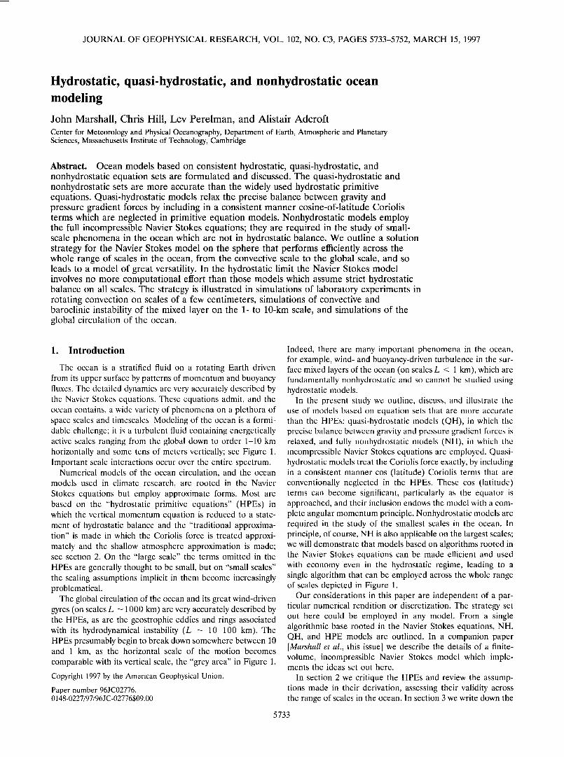
The ocean is a stratified fluid on a rotating Earth driven from its upper surface by patterns of momentum and buoyancy fluxes. The detailed dynamics are very accurately described by the Navicr Stokes equations. These equations admit, and the ocean contains, a wide variety of phenomena on a plethora of space scales and timescales. Modeling of the ocean is a formi- dable challenge; it is a turbulent fluid containing energetically active scales ranging from the global down to order 1-10 km horizontally and some tens of meters vertically; see Figure 1. Important scale interactions occur over the entire spectrum.

Numerical models of the ocean circulation, and the ocean models used in climate research, are rooted in the Navier

Stokes equations but employ approximate forms. Most are based on the "hydrostatic primitive equations" (HPEs) in which the vertical momentum equation is reduced to a statement of hydrostatic balance and the •'traditional approximation" is made in which the Coriolis force is treated approximately and the shallow atmosphere approximation is made; see section 2. On the •'large scale" the terms omitted in the HPEs are generally thought to be small, but on "small scales" the scaling assumptions implicit in them become increasingly problematical.

The global circulation of the ocean and its great wind-driven gyres (on scales L •--1000 km) are very accurately described by the HPEs, as are the geostrophic eddies and rings associated with its hydrodynamical instability (L --• 10-100 km). The HPEs presumably begin to break down somewhere between 10 and I km, as the horizontal scale of the motion becomes

comparable with its vertical scale, the "grey area" in Figure 1.

Copyright 1997 by the American Geophysical Union.

Paper number 96JC02776. 0148-0227/97/96J C-02776509.00

Indeed, there are many important phenomena in the ocean, for example, wind- and buoyancy-driven turbulence in the surface mixed layers of the ocean (on scales L < 1 km), which are fundamentally nonhydrostatic and so cannot be studied using hydrostatic models.

In the present study wc outline, discuss, and illustrate the use of models based on equation sets that are more accurate than the HPEs: quasi-hydrostatic models (QH), in which the precise balance between gravity and pressure gradient forces is relaxed, and fully nonhydrostatic models (NH), in which thc incompressible Navier Stokes equations are employed. Quasi- hydrostatic models treat the Coriolis force exactly, by including in a consistent manner cos (latitude) Coriolis terms that are conventionally neglected in the HPEs. These cos (latitude) terms can becomc significant, particularly as the equator is approached, and their inclusion endows the model with a complete angular momentum principle. Nonhydrostatic models arc required in the study of the smallest scales in the ocean. In principle, of course, NH is also applicable on the largest scales; we will demonstrate that models based on algorithms rooted in the Navier Stokes equations can be made etficient and used with economy even in the hydrostatic regime, leading to a single algorithm that can be employed across the whole range of scales depicted in Figure 1.

Our considerations in this paper are independent of a particular numerical rendition or discretization. The strategy set out here could be employed in any model. From a single algorithmic base rooted in the Navier Stokes equations, NH, QH, and HPE models are outlined. In a companion paper [Marshall et al., this issue] we describe the details of a finite- volume, incompressible Navier Stokes model which imple- ments the ideas set out here.

In section 2 we critique the HPEs and review the assumptions made in their derivation, assessing their validity across the range of scales in the ocean. In section 3 we write down the

5733

5734 MARSHALL ET AL.' HYDROSTATIC AND NONHYDROSTATIC OCEAN MODELING

L ~ 1 m I km 10 km 1,000 km 10,000 km

gravity convection geostrophic gyres global waves 'eddies' circulation

NON-HYDRQ .............................................................................................. HYDROSTATIC

Figure 1. A schematic diagram showing the range of scales in the ocean. Global/basin-scale phenomenon are fundamentally hydrostatic; convective processes on the kilometer scale are fundamentally nonhydrostatic. Somewhere between the ge0strophic and convective scales (10 km to 1 km) the hydrostatic approximation breaks down: the "grey area" in the figure. Models which make the hydrostatic approximation are designed for study of large-scale processes but are commonly used at resolutions that encroach on this grey area (the left- pointing arrow). Nonhydrostatic models based on the incompressible Navier Stokes equations are valid across the whole range of scales but in oceanography have been hitherto used for process studies on the convective scale. We show in this paper that the computational overhead incurred by employing the unapproximated equations is slight in the hydrostatic limit. Thus models rooted in the Navier Stokes equations can also be used with economy for study of the large scale (the right- pointing arrow in the figure).

Navier Stokes equations on the sphere and discuss hydrostatic, quasi-hydrostatic, and nonhydrostatic regimes. Section 4 is concerned with the diagnosis of the pressure field required to ensure that the evolving velocity field remains nondivergent. In HPE and QH a two-dimensional (2-D) elliptic equation must be inverted for the surface pressure; in NH a three- dimensional (3-D) elliptic equation must be inverted subject to Neumann boundary conditions. A strategy is developed for the NH 3-D inversion which exploits the fact that in many (and pe•rhaps most) cases of interest the pressure field is "close" to one of hydrostatic balance and can be used as the starting point of an iterative procedure. Thus the pressure field is separated into surface, hydrostatic, and nonhydrostatic components, and each part is treated separately, greatly speeding the inversion process. In section 5, NH, HPE, and QH models are illustrated in the context of three oceanographic examples, chosen for their interest: simulations of laboratory experiments in rotating convection using NH, simulations of convective and baroclinic instability of the mixed layer using NH, and simulations of the global circulation of the ocean using HPE, NH, and QH. This latter experiment was driven by analyzed winds and fluxes during the period 1985-1995 and the sea surface elevation of the model compared with the TOPEX/POSEIDON altimeter.

We conclude that models can be constructed based on al-

gorithms rooted in the incompressible Navier Stokes equations

which perform efficiently across the whole range of scales in the ocean, from the convective to the global scale. Navier Stokes models are specifically designed for the study of small- scale phenomenon such as convection. But when deployed to study hydrostatic scales, they need be no more demanding computationally than hydrostatic models. Equation sets based on more approximate forms, QH and HPE, are readily implemented as special cases of NH. A comparison of integrations of HPE, QH, and NH at large scale (1 ø horizontal resolution) gives essentially the same numerical solutions. The neglect of cos qb Coriolis terms is the most questionable assumption made by the HPEs, but we find that their inclusion (in QH and NH) yields differences in horizontal currents in ocean gyres of only a few millimeters per second. Thus it is clear that solutions based on the HPEs are not grossly in error. Nevertheless, models based on QH (or NH) should be preferred in studies of large-scale phenomenon.

Finally, we have attempted here, as far as is possible, to present an account which does not make strong assumptions about particular numerical choices. Details of the data- parallel, finite-volume, incompressible Navier Stokes model used here to illustrate our ideas are given by Marshall et al. [this issue]. The mapping of the algorithm onto parallel machines, in data-parallel FORTRAN on the Correction Machine (CM5) and in the implicitly parallel language Id on the data- flow machine MONSOON, is described by Arvind et al. (A comparison of implicitly parallel multi-threaded and data- parallel implementations of an ocean model based on the Navier Stokes equations, submitted to Journal of Parallel and Distributed Computing, 1996) (hereinafter referred to as Arvind et al., submitted manuscript, 1996).

2. Critique of the Hydrostatic Primitive Equations

The HPEs, which assume a precise balance between the pressure and density fields, are almost axiomatic to many me- teorologists and oceanographers. They are widely used in numerical weather forecasting and climate simulations of both the atmosphere and ocean. The terms omitted from the full Navier Stokes equations are customarily thought to be small on large scales (see Lorenz [1967] and Phillips [1973] for good discussions). However, the HPEs preclude the study of nonhydrostatic small-scale phenomena, such as deep convection, the understanding of which is of great importance to climate. The HPEs can also be criticized because of their approximate treatment of the Coriolis force which denies them a full angular momentum principle. Indeed, of the assumptions made in their derivation, the neglect of horizontal Coriolis terms seems the least comfortable. Only very recently have global atmospheric models been developed which relax the hydrostatic approximation (so-called quasi-hydrostatic (OH) models) and include a full treatment of the Coriolis force [see White and Bromley, 1995]). We now critically review, for the purpose of designing a model for the accurate prediction and study of ocean currents from kilometer scales up to the global scale, the treatment of inertial and Coriolis terms in the HPEs.

2.1. Hydrostatic Approximation

Let us inquire into the condition for the neglect of inertial accelerations in the vertical momentum equation. We thus write the inviscid vertical momentum equation in Boussinesq form:

MARSHALL ET AL.: HYDROSTATIC AND NONHYDROSTATIC OCEAN MODELING 5735

Dw 1 asp + 6=0

Dt iOref 0 Z

where 8p denotes a deviation from a hydrostatically balanced reference state at rest, Pref is a standard (constant) value of density, b = -9(t•iO/iOref) is the buoyancy (see Appendix), and D/Dt is the total derivative. The condition for the neglect of Dw/Dt in (1) is that it should be much smaller than b. For simplicity we assume in the following scaling that the local time derivative is of the same order as, or smaller than, the advective terms.

Consider a phenomenon which has a characteristic horizontal scale L and vertical scale h with horizontal and vertical

velocity scales U and W, respectively. The timescale of a particle of fluid moving through the system is of order L/U and a consideration of the buoyancy equation

Db + N2w = 0

Dth

where N 2 = - (#/Pref) (0 p/O Z) is the Brunt-Vaisala frequency of the ambient fluid and D/Dt h is the horizontal component of the total derivative, suggests that a typical vertical velocity will be w • bU/LN 2. Hence Dw/Dt << b if

U 2

L 2N2 %% 1

and should be compared with the familiar condition for the validity of the hydrostatic approximation that compares the frequency of a wave motion, to, with N [see Gill, 1982, section 11.9]. In the above, U/L appears in the place of to. If the advective timescale is short relative to the buoyancy period, then nonhydrostatic effects cannot be neglected. The criterion can also be usefully expressed in terms of the aspect ratio of the motion system 3' = h/L and the Richardson number R, = N2h2/U 2. The motion will be hydrostatic if

3'2 n: (2)

where we can call n the nonhydrostatic parameter. In hydrostatic systems such as the HPEs, (2) is assumed to

be true at the outset and strict balance between gravity and vertical pressure gradient is imposed. Then, because Dw/Dt -= 0, w cannot now be obtained prognostically from (1) but must be diagnosed from the continuity equation. If the stratification is strong and the flow weak (large Ri), then the hydrostatic condition may still be a good one even if 3' is not small. For example, in laboratory experiments 3', dictated by the geometry of the apparatus, is often of order unity; see the simulation of the laboratory experiment in section 5. Nevertheless, the flow can still be hydrostatic if the fluid is sufficiently stratified. In the main thermocline of the ocean the Richardson number is large ("•102-103) and the aspect ratio of the motion is small (0.1- 0.01) and so (2) is well satisfied. But it clearly breaks down in weakly stratified conditions on small horizontal scales; see, for example, the study of the oceanic convective scale (-1 km) in neutral conditions by Jones and Marshall [1993]. There nonhydrostatic models were employed in which, quite naturally, w is obtained by stepping forward (1).

With the increasing power of modern computers, ocean models based on the HPEs are now commonly employed with horizontal resolutions comparable to the depth of the ocean (indeed the need to adequately resolve the geostrophic eddy

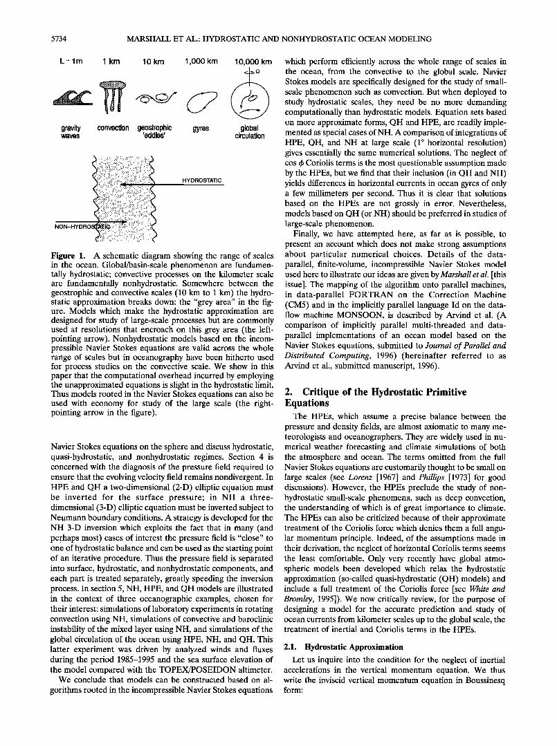
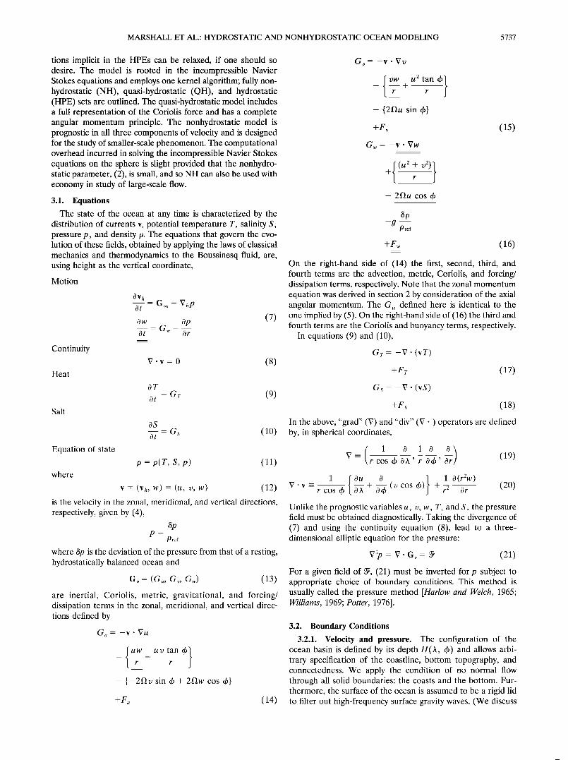
Figure 2. Computation of the axial angular momentum of a particle of mass m at a radius r from the center of the Earth. The latitude is 4> and the longitude X. The spherical polar velocities (u, v, w), equation (4), are also indicated.

scale -10 km demands such high resolutions). In those places where the water column is weakly stratified, the condition (2) may not be adequately satisfied and the appropriateness of the HPEs may be brought into question.

Finally, it should be mentioned that the tiPEs have been criticized because their neglect of the time derivative leads to them being ill-posed when used with open boundaries: see Browning et al. [1990] and Mahadevan et al. [1996a, b]. Instead, these authors recommend the use of a Nit set, but one which is "scaled" to alleviate demands on accuracy in numerically evaluating terms in the vertical momentum equation when the flow is close to geostrophic and hydrostatic balance. The ill- posedness of the HPEs does not go unchallenged, however; see Norbury and Cullen [1985].

2.2. Traditional Approximation

The HPEs make assumptions other than hydrostatic balance. The derivation of the HPEs from the component equations of motion involves a series of approximations and the neglect of various other small terms leading to what has become known as the "traditional approximation." The most problematical assumption is the neglect of the "horizontal Co- riolis terms" (those involving 2D cos &). Their importance and the difficulty of consistently including them in the HPEs have been discussed by Phillips [1966, 1973], Vetohis [1968], and Gill [1982]. White and Bromley [1995] argue that the horizontal Coriolis terms may not always be negligible for synoptic-scale motions in the atmosphere, especially in low latitudes, and they are now included in the "Unified Model" of the United King- dom Meteorological Otfice.

The important issues can readily be understood by consid- ering the axial angular momentum of a particle of fluid of mass m about the rotation axis of the Earth; see Figure 2:

5736 MARSHALL ET AL.: HYDROSTATIC AND NONHYDROSTATIC OCEAN MODELING

DA • Dt = r cos 4> {net zonal force on parcel}

or

with

DA x { l m Op } Dt = r cøs 4> rnFx- (3a) r COS qb Pref 03•

Ax = m{(Dr cos 0 + u)r cos 0} (3b)

the angular momentum and D/Dt the total derivative. Here 4> is the latitude, ,k is the longitude, r is the radius, D

is the angular speed of rotation of the Earth, u is the zonal speed of the particle, and F;, is the zonal component of the frictional force per unit mass. By using the definitions

D2t

u =rcos4> Dt

DO v = r Dt (4)

Dr

(3a) and (3b) directly yield the full zonal momentum equation

Du uw u v tan 4> + - 2Dr sin 4> + 2•w cos 4>

Dt r r

• Op + - (5) 9rcfr cos 0 0h - F x

It is clear from this derivation that to ensure that a model has

a full angular momentum principle, all the terms in (5) must be retained. As is well known and argued, however, the HPEs employ a carefully chosen approximation to (5) in which the underlined terms are neglected. The term 2•w cos 4>, however, is probably not always negligible.

In the tropical oceans, typical vertical velocities approach the continuity limit Uh/L. The 2Dw cos 4> term in (5) is then negligible compared to Du/Dt if

2Dh cos 4> << 1 (6) U

Supposingh -- 100 mandU = 10 cms J, typical of equa- torial jets, for example, the left-hand side is about 0.1 x cos 0 which would suggest that its neglect in quantitative (as op- posed to theoretical) study is unacceptable. It is clear, for example, that the neglect of cos 0 Coriolis terms in the HPEs is much more problematical than the neglect of Dw/Dt in the vertical momentum equation.

The cos 0 Coriolis terms are intimately related to the full spherical geometry of the oceans and atmosphere and tran- scend the approximate quasi-2-D spherical geometry of hydrostatic models (where the shallow atmosphere approximation is made). An implication of this close relationship is that it is very difficult to investigate the effect of the cos 0 terms on familiar problems which, in Cartesian geometry, may be treated ana- lytically in their absence. Attempts to do so lead to nonsepa- rable differential equations even in simple cases such as wave motion in an isothermal atmosphere at rest [Eckart, 1960].

The physical meaning of the 2Dw cos 0 term in (5) is readily understandable as representing the conservation of axial an-

gular momentum as a particle moves vertically in the absence of external couples; see Figure 2. Consider the balance

Du

D-T + 2Dw cos 0 = 0

Since w = Dr/Dr, the above implies that for a particle moving zonally

u + 2Dr cos 0 = const or

8u = -2DSr cos O

for small changes 8. Consider now the consequence of a zonal jet at the equator rising vertically. It acquires a retrograde velocity of 1.2 cm s- 1 for every 100 m it moves vertically, simply by virtue of changing its distance from the axis of rotation of the Earth, an effect which is absent from the HPEs.

The most compelling reason for the neglect of 2Dw cos 4> in the zonal momentum component of the HPEs is that because they assume strict hydrostatic balance and hence neglect the 2Du cos 4> term in the vertical momentum equation, for energetic consistency 2•w cos 4> must also be neglected in the horizontal momentum equation (5), even though the term becomes uncomfortably large as the equator is approached. For these reasons, White and Bromley [1995] advocate the use of a quasi-hydrostatic equation set for global atmospheric modeling that fully represents the Coriolis force but still neglects the Dw/Dt term in (1); this is the QH approximation; see section 3.

Perhaps the key factor determining whether 2• cos 4> terms are important is the stratification, which can suppress vertical motion if it is strong enough. But N is rather small in large volumes of the ocean (mixed layers, for example, and particularly the very deep mixed layers created by wintertime convection). It would seem desirable, then, that any model should have the facility to represent the 2D cos 4> terms.

Finally, one further point must be made. It is clear that the full representation of the Coriolis force, including its horizontal as well as vertical components, is only dynamically consistent if one takes account of the changing position of a particle of fluid from the axis of rotation (in (3b), for example, r should not be replaced by a constant reference value). Thus, to be strictly correct, the "shallow atmosphere" approximation must also be relaxed if horizontal Coriolis terms are to be included:

division by r in (5) retained rather than (as assumed in the HPEs) replaced by a mean radius of the Earth. Nevertheless, several authors have been content to write QH forms in which

r is replaced by a; see the correspondence in Journal of Atmo- spheric Sciences between Phillips [1968], Veronis [1968], and Wangsness [1970], for example. However, it can be shown these shallow atmosphere forms lack a potential vorticity conservation law as well as an angular momentum principle [see White and Bromley, 1995].

In summary, then, the quasi-hydrostatic model retains cos 0 Coriolis terms in the zonal and vertical momentum equations, neglects Dw/Dt in the vertical, and does not make the shallow atmosphere approximation.

3. Incompressible Navier Stokes Equations on the Sphere

In view of the considerations outlined in section 2 we de-

velop now an ocean model in which the traditional assump-

MARSHALL ET AL.' HYDROSTATIC AND NONHYDROSTATIC OCEAN MODELING 5737

tions implicit in the HPEs can be relaxed, if one should so desire. The model is rooted in the incompressible Navier Stokes equations and employs one kernel algorithm; fully nonhydrostatic (NH), quasi-hydrostatic (QH), and hydrostatic (HPE) sets are outlined. The quasi-hydrostatic model includes a full representation of the Coriolis force and has a complete angular momentum principle. The nonhydrostatic model is prognostic in all three components of velocity and is designed for the study of smaller-scale phenomenon. The computational overhead incurred in solving the incompressible Navier Stokes equations on the sphere is slight provided that the nonhydrostatic parameter, (2), is small, and so NH can also be used with economy in study of large-scale flow.

3.1. Equations

The state of the ocean at any time is characterized by the distribution of currents v, potential temperature T, salinity S, pressure p, and density 9. The equations that govern the evolution of these fields, obtained by applying the laws of classical mechanics and thermodynamics to the Boussinesq fluid, are, using height as the vertical coordinate,

Motion

Continuity

Heat

Salt

Equation of state

where

OV h

Ot = G•h - Vhp Ow Op

: Gw Ot Or

(7)

V.v=0 (s)

OT -Gr (9) Ot

OS : ot

p - p(T, S, p) (11)

v: w): w)

is the velocity in the zonal, meridional, and vertical directions, respectively, given by (4),

p= iOref

where 6p is the deviation of the pressure from that of a resting, hydrostatically balanced ocean and

are inertial, Coriolis, metric, gravitational, and forcing/ dissipation terms in the zonal, meridional, and vertical directions defined by

Gu = -v' Vu

_ [uw uvtan&} F F

- {-2•v sin & + 2•w cos &}

+Fu (14)

G• = -v ß Vv

vw u 2 tan 0} - {2f•u sin O}

+F•

Gw = -v' Vw

(15)

(u + v2)} + -

+ 2f•u cos qb

8p

Pref

+Fw (16)

On the right-hand side of (14) the first, second, third, and fourth terms are the advection, metric, Coriolis, and forcing/ dissipation terms, respectively. Note that the zonal momentum equation was derived in section 2 by consideration of the axial angular momentum. The G, defined here is identical to the one implied by (5). On the right-hand side of (16) the third and fourth terms are the Coriolis and buoyancy terms, respectively.

In equations (9) and (10),

Gr = -V' (vT)

+Fr (17)

Gs= -V'(vS)

In the above, "grad" (V) and "div" (V ß ) operators are defined by, in spherical coordinates,

(1 0100) V -= - (19) rcosOOX' r OO' Or

l{OuO } 1O(r2w) V.v -- (20) .osO +. Unlike the prognostic variables u, v, w, T, and S, the pressure field must be obtained diagnostically. Taking the divergence of (7) and using the continuity equation (8), lead to a three- dimensional elliptic equation for the pressure:

Vp:

For a given field of 9, (21) must be inverted for p subject to appropriate choice of boundary conditions. This method is usually called the pressure method [Harlow and Welch, 1965; !4511iams, 1969; Potter, 1976].

3.2. Boundary Conditions

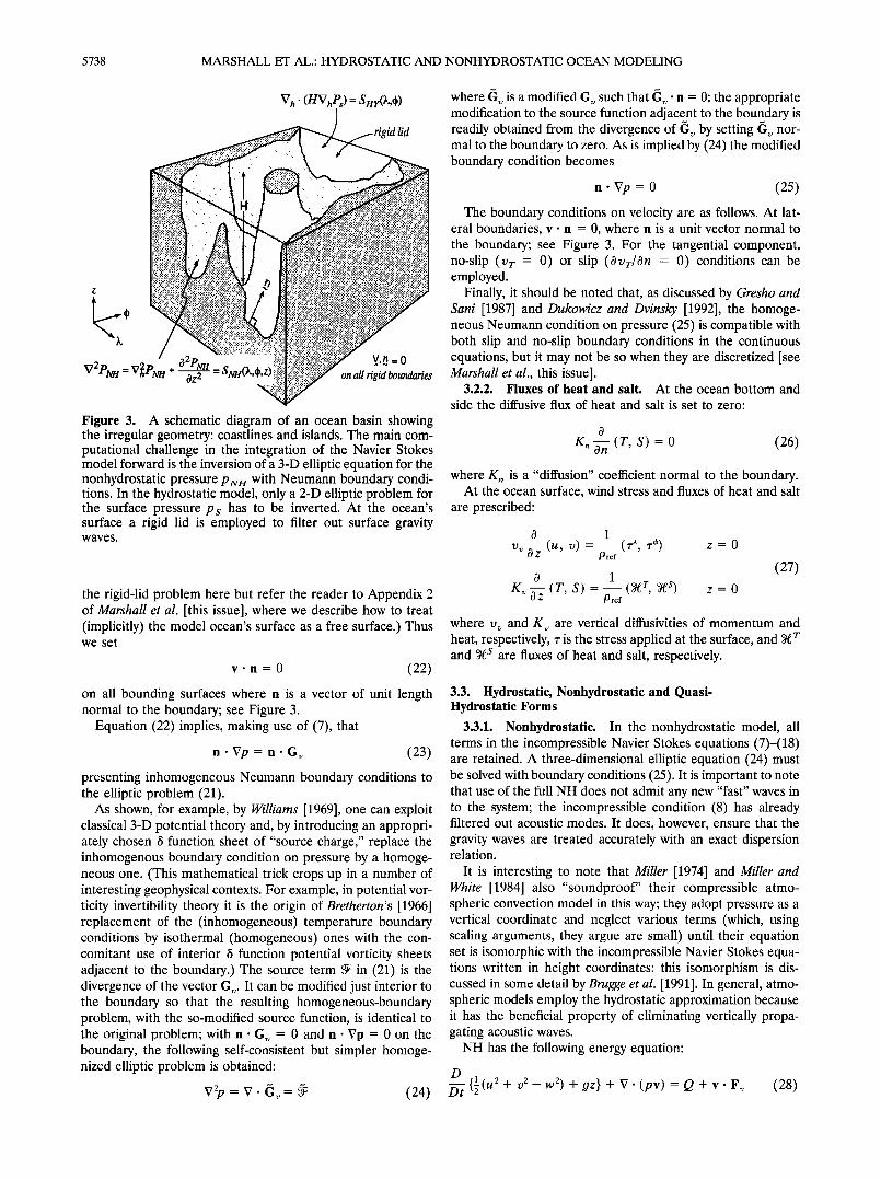
3.2.1. Velocity and pressure. The configuration of the ocean basin is defined by its depth H(X, 0) and allows arbitrary specification of the coastline, bottom topography, and connectedness. We apply the condition of no normal flow through all solid boundaries: the coasts and the bottom. Fur- thermore, the surface of the ocean is assumed to be a rigid lid to filter out high-frequency surface gravity waves. (We discuss

5738 MARSHALL ET AL.' HYDROSTATIC AND NONHYDROSTATIC OCEAN MODELING

V h ' (HVhP ,) = SHy(k,, )

rigid lid

V2PN/-/= Vh2P• + Oz 2 -•'•vH .... * "• -'"•' '"• all rigid boundaries Figure 3. A schematic diagram of an ocean basin showing the irregular geometry: coastlines and islands. The main computational challenge in the integration of the Navier Stokes model forward is the inversion of a 3-D elliptic equation for the nonhydrostatic pressure P NH with Neumann boundary conditions. In the hydrostatic model, only a 2-D elliptic problem for the surface pressure P s has to be inverted. At the ocean's surface a rigid lid is employed to filter out surface gravity waves.

the rigid-lid problem here but refer the reader to Appendix 2 of Marshall et al. [this issue], where we describe how to treat (implicitly) the model ocean's surface as a free surface.) Thus we set

v. n = 0 (22)

on all bounding surfaces where n is a vector of unit length normal to the boundary; see Figure 3.

Equation (22) implies, making use of (7), that

n. Vp = n-G•, (23)

presenting inhomogeneous Neumann boundary conditions to the elliptic problem (21).

As shown, for example, by Williams [1969], one can exploit classical 3-D potential theory and, by introducing an appropri- ately chosen 3 function sheet of "source charge," replace the inhomogenous boundary condition on pressure by a homogeneous one. (This mathematical trick crops up in a number of interesting geophysical contexts. For example, in potential vorticity invertibility theory it is the origin of Bretherton's [1966] replacement of the (inhomogeneous) temperature boundary conditions by isothermal (homogeneous) ones with the con- comitant use of interior 3 function potential vorticity sheets adjacent to the boundary.) The source term • in (21) is the divergence of the vector G•,. It can be modified just interior to the boundary so that the resulting homogeneous-boundary problem, with the so-modified source function, is identical to the original problem; with n.G v = 0 and n- Vp = 0 on the boundary, the following self-consistent but simpler homoge- nized elliptic problem is obtained:

V2p = V. •Jv = • (24)

where Gv is a modified G•: such that G•:. n = 0; the appropriate modification to the source function adjacent to the boundary is readily obtained from the divergence of G•: by setting G•: normal to the boundary to zero. As is implied by (24) the modified boundary condition becomes

n. Vp = 0 (25)

The boundary conditions on velocity are as follows. At lateral boundaries, v. n = 0, where n is a unit vector normal to the boundary; see Figure 3. For the tangential component, no-slip (vr = 0) or slip (Ovr/On = 0) conditions can be employed.

Finally, it should be noted that, as discussed by Gresho and Sani [1987] and Dukowicz and Dvinsky [1992], the homogeneous Neumann condition on pressure (25) is compatible with both slip and no-slip boundary conditions in the continuous equations, but it may not be so when they are discretized [see Marshall et al., this issue].

3.2.2. Fluxes of heat and salt. At the ocean bottom and

side the diffusive flux of heat and salt is set to zero:

0

Kn •nn (T, S) = 0 (26)

where K,• is a "diffusion" coefficient normal to the boundary. At the ocean surface, wind stress and fluxes of heat and salt

are prescribed'

0 1

"v (u, v)=- Pref

0 1

K• • (r, s) = -- (•, •) Pref

z=0

z=0

(27)

where v• and K• are vertical diffusivities of momentum and heat, respectively, r is the stress applied at the surface, and •r and •s are fluxes of heat and salt, respectively.

3.3. Hydrostatic, Nonhydrostatic and Quasi- Hydrostatic Forms

3.3.1. Nonhydrostatic. In the nonhydrostatic model, all terms in the incompressible Navier Stokes equations (7)-(18) are retained. A three-dimensional elliptic equation (24) must be solved with boundary conditions (25). It is important to note that use of the full NH does not admit any new "fast" waves in to the system; the incompressible condition (8) has already filtered out acoustic modes. It does, however, ensure that the gravity waves are treated accurately with an exact dispersion relation.

It is interesting to note that Miller [1974] and Miller and White [1984] also "soundproof" their compressible atmospheric convection model in this way; they adopt pressure as a vertical coordinate and neglect various terms (which, using scaling arguments, they argue are small) until their equation set is isomorphic with the incompressible Navier Stokes equations written in height coordinates: this isomorphism is discussed in some detail by Brugge et al. [1991]. In general, atmospheric models employ the hydrostatic approximation because it has the beneficial property of eliminating vertically propa- gating acoustic waves.

NH has the following energy equation:

D 1 •d 2 Dt {5(u2 + + w2) + !7z} + V. (pv) = Q + v. Fv (28)


where v = (u, v, w) is the three-dimensional velocity vector, Q is the buoyancy forcing, F is the forcing/dissipation term in the momentum equations, and p = (•P/Pref' Note that the pressure work term V ß (pv) vanishes when integrated over the ocean basin if, as assumed here, all bounding surfaces, including the upper one, are assumed rigid.

NH has a complete angular momentum principle as expressed in (3).

3.3.2. Hydrostatic. In HPE, all the underlined terms in (7)-(18) are neglected and r is replaced by a, the mean radius of the Earth. The 3-D elliptic problem reduces to a 2-D one since once the pressure is known at one level (we choose this level to be the rigid lid at the surface), then it can be computed at all other levels from the hydrostatic relation. An energy equation analogous to (28) is obtained except that the contribution of w 2 to the kinetic energy is absent and, on the right- hand side, only forces on the horizontal component of the velocity do work.

The hydrostatic model has an angular momentum principle analogous to (3) but with r replaced by a and the axial angular momentum defined by

A•- m{(fia cos 4> + u)a cos 4>} (29)

Of course, (29) means that the hydrostatic model cannot represent the mechanics contained in (3).

3.3.3. Quasi-hydrostatic. In OH, only the terms underlined twice in (7)-(18) are neglected, and, simultaneously, the shallow atmosphere approximation is relaxed. Thus all the metric terms must be retained and the full variation of the

radial position of a particle monitored. OH has good energetic credentials; they are the same as for HPE. Importantly, however, it has the same angular momentum principle as NH, (3). Again, the 3-D elliptic problem is reduced to a 2-D one. Strict balance between gravity and vertical pressure gradients is not imposed, however, since the 2Du cos O Coriolis term plays a role in balancing g in (16).

4. Hydrostatic, Quasi-Hydrostatic and Nonhydrostatic Algorithms

In HPE and OH the vertical component of the momentum equation becomes a diagnostic relation for the hydrostatic pressure; the vertical velocity is obtained from knowledge of (u, v) using the continuity equation. Instead, in NH, w, just like u and v, is obtained prognostically. In each model the main computational challenge lies in finding the pressure field. In HPE and OH a 2-D elliptic problem must be solved for the pressure at some level surface; in NH the elliptic problem is three dimensional.

4.1. Finding the Pressure Field

If the ocean had a flat bottom, then (24) could readily be solved by projecting p on to the eigenfunctions of the 02/01 '2 operator with boundary condition (25) applied at the (flat) upper and lower boundaries. Then (24) can be written as a set of horizontal Helmholtz equations:

(v, - 4,): 4,) (3o)

where the Greek index labels the vertical eigcnfunction and •, is the corresponding eigenvalue. We can thus separate the 3-D problem (24) into a set of•N, independent 2-D problems, if one truncates at N, vertical modes. The advantage of this procedure is that only one cigenvalue (corresponding to the mode

with no vertical structure) is equal to zero and after appropriate nondimensionalization, all other eigenvalues greatly ex- ceed unity if Az/Ax is small. The Nz - 1 Helmholtz problems are readily solved because the ), term dominates in (30). The 2-D Poisson equation (), = 0 in (30)) presents the main computational challenge. This method of "projection onto modes" is employed, for example, by the nonhydrostatic process model of Brugge et al. [1991], used for studies of convection in flat- bottomed boxes. One cannot directly employ such a modal approach here, where we are concerned with a geometry which is as complex as that of an ocean basin, because with a nonflat bottom the 3-D problem cannot be separated into independent 2-D problems; the modes "interact" through topography. How- ever, it strongly points to the advantage of separating out, as far as is possible, the depth-averaged pressure field.

4.1.1. Depth-averaged pressure. For an arbitrary function ½ we can define its vertical average •t" as

= ½(x, z) dz )

where H = H(A, O) is the local depth. The vertically averaged gradient operator is then

. 1 V/,H (32) The vertical integral of (7) is then, using the rule (32),

O (HV"•) •, 0t = HG•.,. - [V/.,(Hfi") -p(H)V•H] (33)

Since there can be no net convergence of mass over the water column,

V;,. (HV"/,) = 0 (34)

At this point, and followingB•an [1969], ocean modelers often introduce a stream function for the depth-averaged flow. In- stead, and as argued by Dukowicz et al. [1993], it is advantageous to couch the inversion problem in terms of pressure rather than a stream function. The resulting elliptic equation is better behaved because H, the local depth of the ocean, appears in the numerator rather than the denominator of the coefficients that make up the elliptic operator. Furthermore, the pressure equation demands Neumann conditions (equation (25)), whereas the bounda• conditions on the stream function are Dirichlet and can only be determined by car•ing out line integrals around the boundary. This is a cumbersome and (on a parallel computer) costly task. In contrast, the Neu- mann elliptic equation for the pressure, (24)-(25), occurs naturally in the incompressible Navier Stokes problem.

Combining (33) and (34), we obtain our desired equation for the depth-averaged pressure:

...... H

V-(Hg,,,, )+ (35)

where

(I)(H): V. [p(H)V,,H] (36)

It is now clear that if the ocean has a fiat bottom (H = constant), then q)(H) = 0 and equation (35) does not have any pressure-dependent terms on the right-hand side and can be solved unambiguously for •" But if the depth of the basin varies from point to point, one cannot solve for the depth-


averaged pressure without knowledge of •(H). We can, however, make progress by separating the pressure field into hydrostatic, nonhydrostatic, and surface pressure parts.

4.1.2. Surface, hydrostatic and nonhydrostatic pressure. Let us write the pressure p as a sum of three terms:

p(X, &, z) = ps(X, &) + pro-(X, ok, z) + PNH(X, d), z) (37)

The first term, P s, only varies in the horizontal and is independent of depth. The second term is the hydrostatic pressure defined in terms of the weight of water in a vertical column above the depth z,

pro-(X, &, z) = - • dz' (38a)

where

•--•-P-{(u2+v2)}-211ucosck (38b) • = •/ Pref r

Note that (38a) and (38b) are a generalized statement of hydrostatic balance, balancing vertical pressure gradients with a "reduced gravity" and, in QH, modified by Coriolis and metric terms also.

It should be noted that the pressure at the rigid lid, p(z - 0), has a contribution from both Ps and PNH (by definition, p• = 0, at z = 0). In the hydrostatic limit, PNH = 0 and Ps is the pressure at the rigid lid.

By substituting (37) into (35), an equation for P s results:

Vh' (nVhps) = •f Hy(•., (•))

ß - Vh(Hp/, ) (39) + Vh [pNn(H)VhH] 2 --.

where '•])HY is given by

b•HV(X, &)= Vh' (HG .H)_ Vh2(Hfi_•H )

+ Vh' [pHv(H)VhH] (40)

In HPE and QH the (doubly) underlined terms on the right- hand side of (39), which depend on the nonhydrostatic pressure, are set to zero, and P s is found by solving

Vh' (HVhps) = b•m-(X, &) (41)

The vertical velocity is obtained through integration of the continuity equation vertically:

f0 w = - Vh'vh dz' (42)

In NH, instead, w is found by prognostic integration of the vertical velocity equation:

OW _ Ow OpN H (43a) Ot Oz

where

Ow = Gw + • (43b)

Note that in (43a) and (43b), the vertical gradient of the hydrostatic pressure has been canceled out with •, (38b), rendering it suitable for prognostic integration; see section 4.2.

We solve (41) to give a provisional solution for Ps and then

find PNH from the elliptic equation obtained by substituting (37) in to (7) and noting, as before, that V ß v = 0 at each point in the fluid:

where

O2pNH V2pNH = V•pN, + OZ 2 = b•N, (44a)

b•s, = !7. P,v- 17•(Ps + Pro,) (44b)

where Q-v = (Gvh, •,•). Equations (44a) and (44b) are solved with the boundary

conditions

17PNH n = 0 (45)

If the flow is close to hydrostatic balance (see section 4.2 below), then the 3-D inversion converges rapidly because PNH is then only a small correction to the hydrostatic pressure field.

The solution PNH to (43) and (44) does not vanish at the upper surface and so refines the pressure at the lid; it is in this sense that the Ps obtained from (41) is provisional. In the interior of the fluid, nonhydrostatic pressure gradients, VpNH, drive motion.

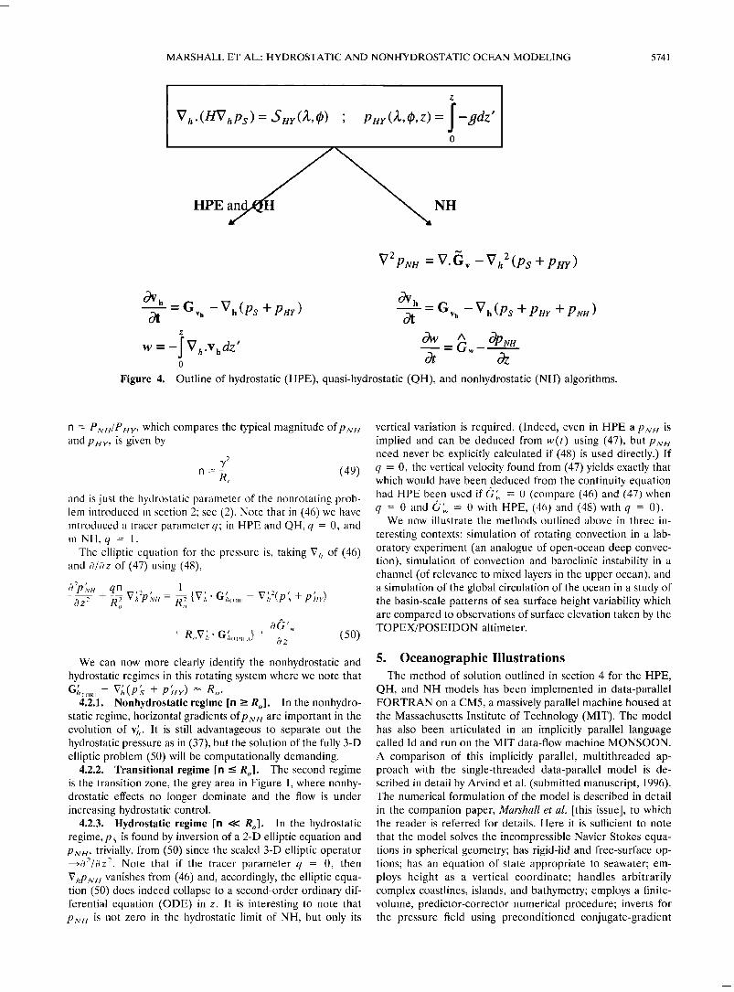
The method of solution employed in the HPE, QH, and NH models is summarized in Figure 4 below. There is no penalty in implementing QH over HPE except, of course, some compli- cation that goes with the inclusion of cos & Coriolis terms and the relaxation of the shallow atmosphere approximation. But this leads to negligible increase in computation. In NH, in contrast, one additional elliptic equation, a three-dimensional one, must be inverted. However, we show that this "overhead" of the NH model is essentially negligible in the hydrostatic limit (as the nonhydrostatic parameter, (2), n --• 0), resulting in a nonhydrostatic algorithm that, in the hydrostatic limit, is as computationally economic as the HPEs.

4.2. Navier Stokes Model in the Hydrostatic Limit

It is important to understand how the NH model performs in the hydrostatic, geostrophic limit. Accordingly, in the Appen- dix we nondimensionalize our model equations and consider the balance of terms if the flow is close to one of hydrostatic and geostrophic balance. For clarity and simplicity we neglect horizontal Coriolis terms in our scale analysis. There are three important nondimensional numbers: the Rossby number R o = U/fL, the Richardson number Ri = N2h 2/U 2, and the aspect ratio of the motion 3/ = h/L. Quasi-geostrophic dynamics occurs on the deformation scale, Nh/f, at large R i and small Ro such that R•Ro 2 • 1.

The nondimensional form of the momentum and continuity equations may be written in terms of Ro, Ri, and •, thus (see Appendix)'

' 1 O'Vh t t t

Ot = G' + {G' - 17h(Ps +P,r+qnpk,)} (46) -• hOTHER •OO hCORI t

NH (47) ow' = O' - op_ Ot' • Oz

OW •

17h' V• + Ro Oz • = 0 (48)

where the prime symbols indicate nondimensional quantities, G•coR I are the sin & Coriolis terms, and G;,OTnE • contain all other contributions, from advection, sources, sinks, etc. Here


V h . (HV hPs ) - ,.5'Hy (•, (p)

z

Put (2,, 0, z) - I -g&' 0

HPE NH

V2p•vu - V. Gv -Vh (Ps + Put)

ODVh : G v h - Vh (Ps + Put) O•Vh = G • • v• -- Vh (Ps + Put + P.u )

W---- Vh.¾hdZ' O,qt =Gw-• o Figure 4. Outline of hydrostatic (HPE), quasi-hydrostatic (OH), and nonhydrostatic (NH) algorithms.

n = P,,vn/P,r, which compares the typical magnitude ofp•v, and P,v, is given by

n--R, (49) and is just the hydrostatic parameter of the nonrotating problem introduced in section 2; see (2). Note that in (46) we have introduced a tracer parameter q; in HPE and OH, q = (), and in NH, q = 1.

The elliptic equation for tiao pressure is, taking V/, of (46) and O/•,z of (47) using (48),

qn , 1 , a•P;"+ -,, v;,•p,•,,: • Iv,,. •' - v;,:(p', + O z 2 R • R • /'('•

_

+R,Vj,.Gj ......... } + az (50)

We can now more clearly identify the nonhydrostatic and hydrostatic regimes in this rotating system where we note that

4.2.1. Nonhydrostatic regime [nm R,,]. In the nonhydrostatic regime, horizontal gradients ofp,•z z are important in the evolution of v;,. It is still advantageous to separate out the hydrostatic pressure as in (37), but the solution of the fully 3-D elliptic problem (50) will be computationally demanding.

4.2.2. Transitional regime [n • Re]. The second regime is the transition zone, the grey area in Figure 1, where nonhydrostatic effects no longer dominate and the flow is under increasing hydrostatic control.

4.2.3. Hydrostatic regime [n << Re]. In the hydrostatic regime, P•s is found by inversion of a 2-D elliptic equation and p,•, trivially, from (50) since the scaled 3-D elliptic operator •2/0Z2. Note that if the tracer parameter q = 0, then Vz, p•, vanishes from (46) and, accordingly, the elliptic equation (50) does indeed collapse to a second-order ordinary differential equation (ODE) in z. It is interesting to note that p•,, is not zero in the hydrostatic limit of NH, but only its

vertical variation is required. (Indeed, even in HPE a p^f, is implied and can be deduced from w(t) using (47), but P/v, need never be explicitly calculated if (48) is used directly.) If q •- 0, the vertical velocity found from (47) yields exactly that which would have been deduced from the continuity equation had HPE been used if •i• • 0 (compare (46) and (47) when q - 0 and •;' • 0 with HPE, (46) and (48) withq : 0).

We now illustrate the methods outlined above in three in-

teresting contexts: simulation of rotating convection in a laboratory experiment (an analogue of open-ocean deep convection), simulation of convection and bareclinic instability in a channel (of relevance to mixed layers in the upper ocean), and a simulation of the global circulation of the ocean in a study of the basin-scale patterns of sea surface height variability which are compared to observations of surface elevation taken by the TOPEX/POSEIDON altimeter.

5. Oceanographic Illustrations The method of solution outlined in section 4 for the HPE,

QH, and NH models has been implemented in data-parallel FORTRAN on a CM5, a massively parallel machine housed at the Massachusetts Institute of Technology (MIT). The model has also been articulated in an implicitly parallel language called Id and run on the MIT data-flow machine MONSOON.

A comparison of this implicitly parallel, multithreaded approach with the single-threaded data-parallel model is described in detail by Arvind et al. (submitted manuscript, 1996). The numerical formulation of the model is described in detail

in the companion paper, Marshall etal. [this issue], to which the reader is referred for details. Here it is sufficient to note

that the model solves the incompressible Navier Stokes equations in spherical geometry; has rigid-lid and flee-surface options; has an equation of state appropriate to seawater; employs height as a vertical coordinate; handles arbitrarily complex coastlines, islands, and bathymetry; employs a finite- volume, predictor-corrector numerical procedure; inverts for the pressure field using preconditioned conjugate-gradient


Figure 5. Domain decomposition used in the data-parallel model. The schematic diagram shows our fluid contained in an ocean basin decomposed into columns distributed over 16 pro- cessors of a parallel computer. The thick black lines indicate regions of the domain assigned to the same processor. The thin lines indicate the number of "volumes" within each subdo- main.

methods; has HPE, NH, and OH options; and is designed specifically to exploit parallel computers.

The numerical scheme ensures that the evolving velocities be divergence free by solving our Poisson equation for the pressure with Neumann boundary conditions and then using these pressures to update the velocities. The equations are discretized using finite-volume methods. Regular volumes based on a uniform discretization of longitude, latitude, and depth are employed. When they abut the bottom or coast, the volumes may take on irregular shapes and be "sculptured" to fit the boundary, improving our representation of coastlines and topography; see Adcroft et al. [1996].

The model lends itself very naturally to parallel computation. Most of the parallelism is fine-grained data parallelism, available on the order of the total number of grid cells in the computational domain. The only exception is the diagnostic inversion for the pressure field which involves global reduc- tions across all the cells of the domain. The model has been

developed in a data-parallel FORTRAN on the 128-node CM5 available to us at MIT which enables one to exploit the data locality and regular structure of the model grid. In our approach the physical domain is decomposed by allocating equally sized vertical columns of the ocean to each processing unit. For example, given a typical 200 x 200 x 30 three- dimensional spatial grid representing an ocean basin, say, it is straightforward to carve the grid in to 128 domains, each one with roughly 12,000 points in a 20 x 20 • 30 network, each handling the computation in that sector of the ocean from the surface to the bottom; see Figure 5. The key to the success of this relatively simple decomposition is its role in reducing the overhead of the potentially costly task of diagnosing the pressure field.

Regardless of the specifics of any discrete approximation to

the gradient and divergence operators, (19) and (20), which are required to step forward the fluid equations, solving the pressure Poisson equation at each time step is computationally expensive because this involves communication between pro- cessors. But as we shall see, the overhead incurred by NH in solving (43a) and (43b) for PN, is not severe provided the nonhydrostatic parameter n, (49), is sufficiently small. This is true even in the highly irregular geometries of an ocean basin, provided that P s is first obtained in a 2-D solve. Thus in the hydrostatic limit, NH is not more demanding of computational resources than HPE or OH. To invert the 3-D Poisson equation for the pressure field, a block preconditioned conjugate- gradient algorithm is employed. The preconditioner used is the inverse of 02/0252 [see Marshall et al., this issue], to which the 3-D elliptic operator asymptotes in the hydrostatic limit. The preconditioning equations are solved using "lower/upper" ("LU") decomposition which inverts 02/OZ 2 for each vertical column in the ocean. Thus repeated multiplication by the preconditioner does not involve any communication between pro- cessors. Furthermore, in computing the matrix-vector products needed in each conjugate-gradient (CG) iteration, only near- est-neighbor communication is required because the 128 domains are arranged so as to take advantage of the direct links in the CM5's fat-tree based communication network. The

model is presently achieving a sustained performance of 3 Gflops on the 128-node machine.

The model has been employed to study a number of phenomena whose scales range from centimeters (in simulations of laboratory experiments) up to many thousands of kilometers (in simulations of the evolution of the sea surface elevation over the globe). We briefly present three studies that have been recently carried out to demonstrate the capabilities of the model: (1) simulations of laboratory experiments carried out by Jack Whitehead at Woods Hole in a 1 m x 1 m x 30 cm rotating tank, in which the aspect ratio 3' • 1; (2) convection and baroclinic instability in a periodic channel, of dimension 50 km x 20 km x 2 km, in which 3' • 0.1; and (3) circulation of the global ocean on decadal timescales in a basin with realistic geography and bathymetry; here 3' • 10-3. Experi- ments 1 and 2 use NH; experiment 3 has used HPE, NH, and OH. The same kernel algorithm, however, is used in all cases. Model resolutions and parameters are summarized in Table 1.

5.1. Laboratory Experiment

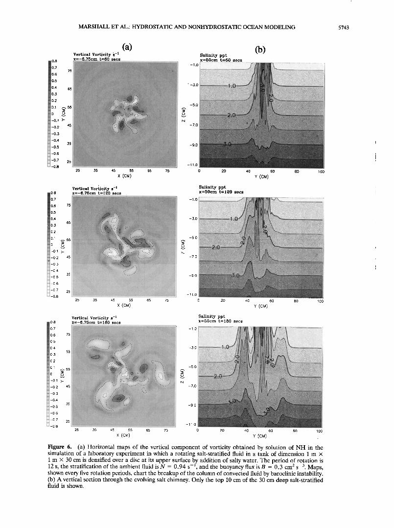
Figure 6a shows the distribution at the surface of the vertical component of vorticity 60 s (five rotation periods) after a continuous source of salinification was applied over a circular patch of radius 10 cm at the upper surface of a numerical simulation of rotating convection into a salt-stratified fluid. The laboratory experiments are described by Whitehead et al. [1996] and were used to explore the mechanisms at work in the convective overturning of a stratified ocean driven by buoyancy loss from an extended but confined region at its upper surface.

Table 1. Typical Values of Stratification N and Coriolis Parameter f for the Three Experiments Discussed in the Text

N, s -• f, s -• L, m h, m U, m s -• R i -- N2H2/U2 R o = U/fL 3' = H/L

Laboratory 30 6 1-5 x 10 -3 10 -2 10 -2 10-•-10 1 1 Mixed layer 5 X 10 -4 10 -4 1-5 x 103 2 X 103 10-2-10 -1 10-•-10 10-•-1 0.2-1 Global currents 10 -2 10 -4 5-10 x l0 s 5 x 103 10-•-1 103 10 -3 10 -3

Also shown are our estimates of the length scales (in the horizontal L and vertical h) and typical speeds U associated with the phenomenon observed in the numerical experiments. R i is the Richardson number, R o is the Rossby number, and •/is the aspect ratio.


75

65

45

35

25

(a) Vertical Vorticity b-1 z=-6.75em t=60 seca

I "'•"• ;' ""• •: -'"•'" ' -'"'-" ' '7'"'• '•' •• •::•'• "' "•"" •• *'"'" "' '"•'•' • '••• -••• ...... • -- g,.-.:!• ....- ................ ,,,.,.,....,....,...••,,,,,.••,,.,•••..•i:•...,....,,,,,,.o•,••.,••.• •

25 35 45 55 65 75

X (CM)

-1.0

ß -3.0

-5.0

-7.0

-9.0

-11.0

0

(b) Salinity ppt x=50cm t=60 sees

ß

2O 4O 60 80 1 O0

Y (CM)

65 0.3

k•0.2 0

-0.1 >- -0.2 45

0-3 -0.4 -0.5

-0.6

-0.7 25 -0.8

Vertical VorUcity s -• Salinity ppt z=-6.75cm t=120 seca x=50cm t=120 seca

/

:o:.:.: ¾.•,-.. ¾ . ß ..::•¾ -.:.:.. •.•.}:..,.....&<...., o •'":'•,•:•>.:.• '• •'.4.o.: •:'::•. *:- • F•"•':':'- "•:':': ':-,•'. '-':-:-:"-':':', .• •?..• ::-';

...... •:-.• ½•?•.t-'i•! ..:•::-":.. •ii:½i:i,•,i,::::i::-'. •'•- •:<.- ,. •...'..'!..?

•"'" '""•:•:••••• {•': <"'"" •- ß '-'"•- -" ½"•.:-' • :'¾/"--? :• :•...i...-"•..*.": •: '• * •: •: r'" ........... ..... = *' '"'"'"'""• <"• ;••- :••/ii :¾::: '•: .......... "• """ '"'"'"'"'""'•'"'"'"••••--'"••iii'-"'-'"'"""'"' '•'" ß '"""'":•':"' "•:"-- '••••!ii• ....... ½•:-•:••..--.'.-"•'•'"'"'""•'""•"•:••:-..• - •'ø

............. .--•.: ...................... •i,•2, ........ '-:.'.':•-•i,,,J - • •.0 25 35 45 55 65 75 0 20 40 60 80 100

x (c•) Y (CM)

Vertical Vortieity s -I Salinity ppt ..... 0.8 z=-6.75cm t=lg0 sees x=50cm t=180 seca

i:•,•. ¾:::•---- *, --;... J-'"....."•.!•.-';•....• ......... • ' ½'"'"••••••'-.:iI -,.o :• ............................................................ • ......................... ::::!• ............. - .................. - ...................... •: •: •: •: •:•:• ......... •: •: •:•:• ....................... :......o :...,.•:: .x./•... 5:•..?;• ::.q::.¾...•¾•.:....:.o• •::.o.::::::::..•.-.-,....:.-•,:•:•œ½..x:.:• ........ •------- '-----'-'--'-'-'•-.'-:-.••••;•.

:::sr..o.• .-'. ½<. ,;.:.>.'.•,.'.-::.'::::::: .................... ::::::¾..:..r:'•'• •..<5•;,-: '.:.•:.-¾•g.%-'•:%-.:•' •¾s.-:::.-•[-'•:.q::: :-.'-':¾.-¾s'>:-:-....•.•:......-;•'..x.:;•.:..-•

I I :•. o., • I '• ................. "" *'"•"'•'"• '- •••••i "•'"'½½'"'-'" ' '" •' •'•'•••':•••••iI"':'""•""'•'" •-"••1 -•. o

:•-½•"'::':'..---'--•.....' -'•,.'.-'.-•-.'.-' ';-•i ...................... .-?.-::.-ii::.'. r•,;•, ..-4..+,;•.j•. ø.•*•-....-':._..•-'.-'2'•-* >""'"•",,-.,//."•,...-.•....,'•.•:j >;q..,-'."..;;.J.T•' '• ::::::::::::::::::::::::::::::::::: ß Z >.',•.?;• -:g• .•-:•:•'..-'.-::..•rf.-'-,.'.- ß .•..=• ..... g•.:.-. ...... ::: ........ ß ......... •.-.•,.. ..................... •'":'":••••i•., .-..-..-::•..-•.: •;•- -'-'"•i,,.: :•:• -o.• ......... "•"•"'••:•;••:•••[i•:..':::•:•:•:::::•:•:•::,.-• -•:::•:

i ...... ß :-•...,>.[?,,',• r.•./...'.::•:,.- ..... •?,':"'"---½'•*..., ? • ....... ;¾--'.-.•. '•...-'.'.."i.• .............. _:.-_'::•_.'•:: '•4•J...o:o.,½•.....:::f .•:.-¾::•.::, .: ,,... •>• •j.f,..,..:•]. •2.'..' •-'.i• ,' ,- i,-"•. .......... o'"$"':•'½' "•- -- '•- ß --,-"•.-:-"Ji.:::•-'.-'.-:-."-.m .•-..':o.'....-'•.::::.•. :,.:;j..-::.:...?..•o• '$}..-'I• •:•:• o:o>x::p.•x..-.:.:.:.:,. •.q..:::..xo: x ¾$..::::• 2 s •.' ................... •-'"'•"''•'"'"'"'•'"':•' ":•••••••i'"'"'"•'"' '"'"'"•' "':•-- ,••*••••,•:•i' "'"" ""•'"'"'"'"'•':'"••::•-"•••. --'.'i.-".-,." - 11.0 -0.a • ..................................................... - - ----'----"-•"••'""••':•••••••••i:'":::::/

25 35 45 55 65 75 0 20 40 60 80 100

x (CM) ¾ (CM)

Figure 6. (a) Horizontal maps of the vertical component of vorticity obtained by solution of NH in the simulation of a laboratory experiment in which a rotating salt-stratified fluid in a tank of dimension 1 m x 1 m x 30 cm is densifted over a disc at its upper surface by addition of salty water. The period of rotation is 12 s, the stratification of the ambient fluid is N -- 0.94 s -1, and the buoyancy flux is B = 0.3 cm 2 s -3. Maps, shown every five rotation periods, chart the breakup of the column of convected fluid by baroclinic instability. (b) A vertical section through the evolving salt chimney. Only the top 10 cm of the 30 cm deep salt-stratified fluid is shown.


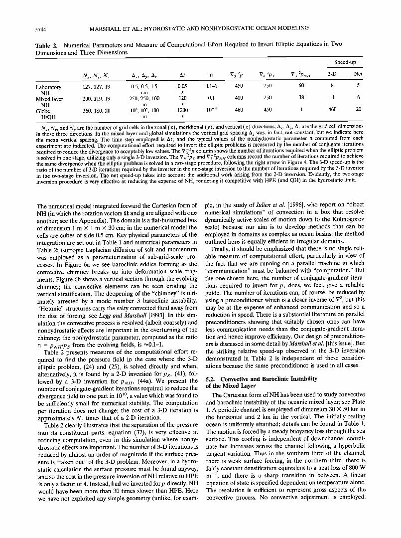
Table 2. Numerical Parameters and Measure of Computational Effort Required to Invert Elliptic Equations in Two Dimensions and Three Dimensions

Speed-up

Nx, Ny, N z Ax, Ay, A z At 13 V•2p V;2ps V•2p•v. 3-D Net Laboratory 127, 127, 19 0.5, 0.5, 1.5 0.05 0.1-1 450 250 60 8 5

NH cm s

Mixed layer 200, 119, 19 250, 250, 100 120 0.1 400 250 38 11 6 NH m s

Globe 360, 180, 20 105, 105, 100 1200 10 -4 460 450 1 460 20 H/QH m s

Nx, Ny, and N z are the number of grid cells in the zonal (x), meridional (y), and vertical (z) directions; Ax, Ay, A z are the grid cell dimensions in these three directions. In the mixed layer and global simulations the vertical grid spacing Az was, in fact, not constant, but we indicate here the mean vertical spacing. The time step employed is At, and the typical values of the nonhydrostatic parameter n computed from each experiment are indicated. The computational effort required to invert the elliptic problems is measured by the number of conjugate iterations required to reduce the divergence to acceptably low values. The V •- 2p column shows the number of iterations required when the elliptic problem is solved in one stage, utilizing only a single 3-D inversion. The V•-2ps and V•-2pNH columns record the number of iterations required to achieve the same divergence when the elliptic problem is solved in a two-stage procedure, following the right arrow in Figure 4. The 3-D speed-up is the ratio of the number of 3-D iterations required by the inverter in the one-stage inversion to the number of iterations required by the 3-D inverter in the two-stage inversion. The net speed-up takes into account the additional work arising from the 2-D inversion. Evidently, the two-stage inversion procedure is very effective at reducing the expense of NH, rendering it competitive with HPE (and QH) in the hydrostatic limit.

The numerical model integrated forward the Cartesian form of NH (in which the rotation vectors II and g are aligned with one another; see the Appendix). The domain is a flat-bottomed box of dimension 1 m x 1 m x 30 cm; in the numerical model the cells are cubes of side 0.5 cm. Key physical parameters of the integration are set out in Table 1 and numerical parameters in Table 2; isotropic Laplacian diffusion of salt and momentum was employed as a parameterization of sub-grid-scale processes. In Figure 6a we see baroclinic eddies forming as the convective chimney breaks up into deformation scale frag- ments. Figure 6b shows a vertical section through the evolving chimney; the convective elements can be seen eroding the vertical stratification. The deepening of the "chimney" is ultimately arrested by a mode number 3 baroclinic instability. "Hetonic" structures carry the salty convected fluid away from the disc of forcing; see Legg and Marshall [1993]. In this simulation the convective process is resolved (albeit coarsely) and nonhydrostatic effects are important in the overturning of the chimney; the nonhydrostatic parameter, computed as the ratio n = PN,/Ps from the evolving fields, is •0.1-1.

Table 2 presents measures of the computational effort required to find the pressure field in the case where the 3-D elliptic problem, (24) and (25), is solved directly and when, alternatively, it is found by a 2-D inversion for Ps, (41), fol- lowed by a 3-D inversion for PN--, (44a). We present the number of conjugate-gradient iterations required to reduce the divergence field to one part in 10 •ø, a value which was found to be sufficiently small for numerical stability. The computation per iteration does not change; the cost of a 3-D iteration is approximately Nz times that of a 2-D iteration.

Table 2 clearly illustrates that the separation of the pressure into its constituent parts, equation (37), is very effective at reducing computation, even in this simulation where nonhydrostatic effects are important. The number of 3-D iterations is reduced by almost an order of magnitude if the surface pressure is "taken out" of the 3-D problem. Moreover, in a hydrostatic calculation the surface pressure must be found anyway, and so the cost in the pressure inversion of NH relative to HPE is only a factor of 4. Instead, had we inverted forp directly, NH would have been more than 30 times slower than HPE. Here

we have not exploited any simple geometry (unlike, for exam-

pie, in the study of Julien et al. [1996], who report on "direct numerical simulations" of convection in a box that resolve

dynamically active scales of motion down to the Kolmogorov scale) because our aim is to develop methods that can be employed in domains as complex as ocean basins; the method outlined here is equally efficient in irregular domains.

Finally, it should be emphasized that there is no single reliable measure of computational effort, particularly in view of the fact that we are running on a parallel machine in which "communication" must be balanced with "computation." But the one chosen here, the number of conjugate-gradient iterations required to invert for p, does, we feel, give a reliable guide. The number of iterations can, of course, be reduced by using a preconditioner which is a closer inverse of V 2, but this may be at the expense of enhanced communication and so a reduction in speed. There is a substantial literature on parallel preconditioners showing that suitably chosen ones can have less communication needs than the conjugate-gradient iteration and hence improve efficiency. Our design of preconditioners is discussed in some detail by Marshall et al. [this issue]. But the striking relative speed-up observed in the 3-D inversion demonstrated in Table 2 is independent of these considerations because the same preconditioner is used in all cases.

5.2. Convective and BarOClinic Instability of the Mixed Layer

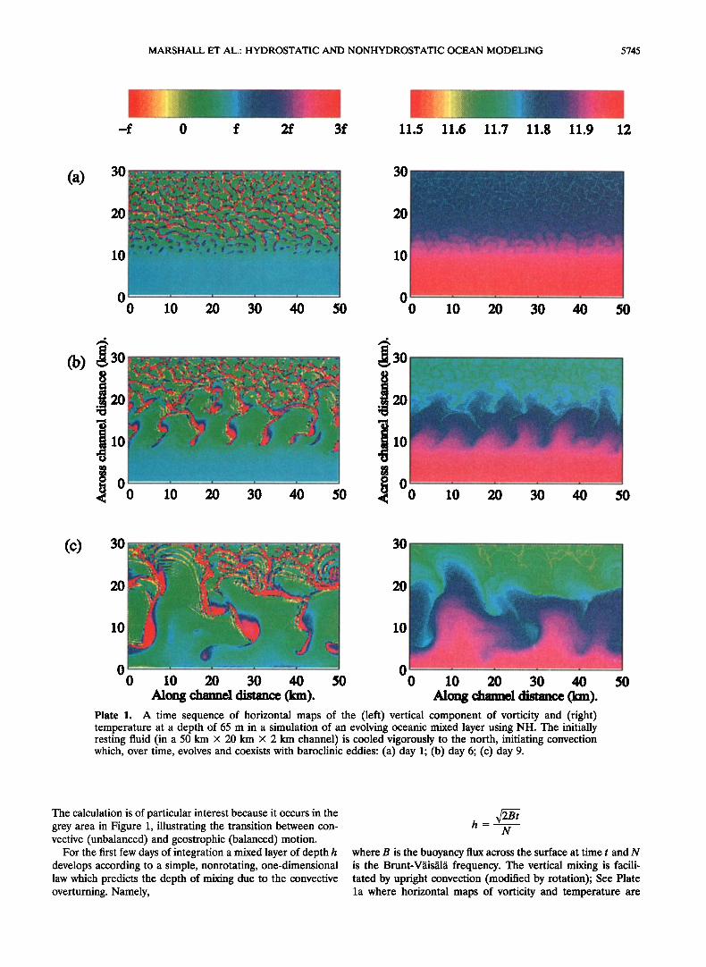
The Cartesian form of NH has been used to study convective and baroclinic instability of the oceanic mixed layer; see Plate 1. A periodic channel is employed of dimension 30 x 50 km in the horizontal and 2 km in the vertical. The initially resting ocean is uniformly stratified; details can be found in Table 1. The motion is forced by a steady buoyancy loss through the sea surface. This cooling is independent of downchannel coordinate but increases across the channel following a hyperbolic tangent variation. Thus in the southern third of the channel, there is weak surface forcing, in the northern third, there is fairly constant densification equivalent to a heat loss of 800 W m -2, and there is a sharp transition in between. A linear equation of state is specified dependent on temperature alone. The resolution is sufficient to represent gross aspects of the convective process. No convective adjustment is employed.


-f 0 f 2f 3f 11.5 11.6 11.7 11.8 11.9 12

30

10

0 10 20 30 40 50 0 10 20 30 40 50

,,

1,o 0 10 20 30 40 50

•30

10 20 30 40 50

30

10

0 '--'-- 0 0 10 20 30 40 50 0 10 20 30 40

Along channel distance (kin). Along channel distance (Inn). Plate 1. A time sequence of horizontal maps of the (left) vertical component of vorticity and (right) temperature at a depth of 65 m in a simulation of an evolving oceanic mixed layer using NH. The initially resting fluid (in a 50 km x 20 km x 2 km channel) is cooled vigorously to the north, initiating convection which, over time, evolves and coexists with baroclinic eddies: (a) day 1; (b) day 6; (c) day 9.

50

The calculation is of particular interest because it occurs in the grey area in Figure 1, illustrating the transition between convective (unbalanced) and geostrophic (balanced) motion.

For the first few days of integration a mixed layer of depth h develops according to a simple, nonrotating, one-dimensional law which predicts the depth of mixing due to the convective overturning. Namely,

where B is the buoyancy flux across the surface at time t and N is the Brunt-Vfiisfilfi frequency. The vertical mixing is facili- tated by upright convection (modified by rotation); See Plate la where horizontal maps of vorticity and temperature are


plotted at day 1. As a result of the developing density gradient across the channel, the flow adjusts to thermal wind balance which becomes baroclinically unstable.

After 6 days a mode six, finite amplitude, baroclinic instability has grown in the channel center and is responsible for exchanging water laterally, from the region of deep mixing to the unconvected fluid and vice versa (Plate lb). In the north the fine plume-scale elements can be seen drawing the buoyancy from the interior. At later times a field of geostrophic turbulence evolves to larger scale as the baroclinic waves "break" laterally (Plate l c). Ultimately, the evolution of the whole layer is profoundly affected by the lateral flux of buoyancy due to baroclinic eddies. The hydrodynamics at play in simulations such as those shown in Plate 1, and its relevance to oceanic mixed layers, are discussed in detail by Haine and Marshall [1996].

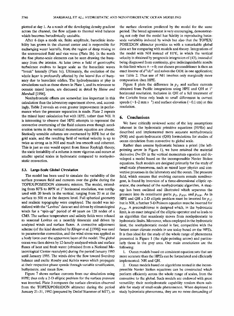
Nonhydrostatic effects are somewhat less important in this calculation than the laboratory experiment above, and, accordingly, Table 2 reveals an even greater improvement in performance when the pressure separation is made. Plate 2 repeats the mixed layer calculation but with HPE, rather than NH. It is interesting to observe that HPE attempts to represent the convective overturning of the fluid column even though accel- eration terms in the vertical momentum equation are absent. Statically unstable columns are overturned by HPE but at the grid scale, and the resulting field of vertical velocity is up to twice as strong as in NH and much less smooth and coherent. This is just as one would expect from linear Rayleigh theory; the static instability of a column is more vigorous and occurs at smaller spatial scales in hydrostatic compared to nonhydrostatic convection.

5.3. Large-Scale Global Circulation

The model has been used to simulate the variability of the surface pressure field and currents over the globe during the TOPEX/POSEIDON altimetric mission. The model, extend-

ing from 80øS to 80øN at 1 ø horizontal resolution, was config- ured with 20 levels in the vertical, ranging from 20 m at the surface to 500 m at the deepest level. Full spherical geometry and realistic topography were employed. The model was initialized with the "Levitus" data set and driven by climatological winds for a "spin-up" period of 40 years on 128 nodes of a CM5. The surface temperature and salinity fields were relaxed to seasonal Levitus on a monthly timescale and driven by analyzed winds and surface fluxes. A convective adjustment scheme (of the kind described by Klinger et al. [1996]) was used to parameterize convection, and the wind stress was applied as a body force over the uppermost layer of the model. The global ocean was then driven by 12-hourly analyzed winds and surface fluxes of heat and fresh water (obtained from a National Me- teorological Center reanalysis) during the period January 1985 until January 1995. The winds drive the flow toward Sverdrup balance and excite Rossby and Kelvin waves which propagate at their respective phase speeds through variable stratification, bathymetry, and mean flow.

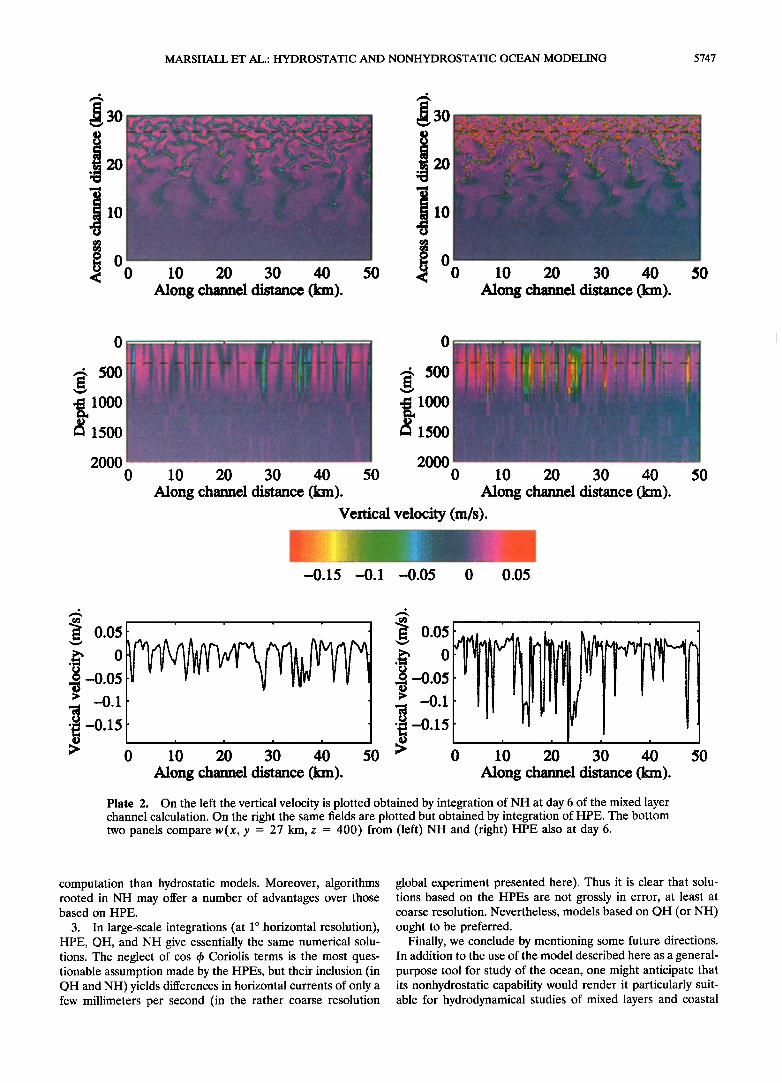
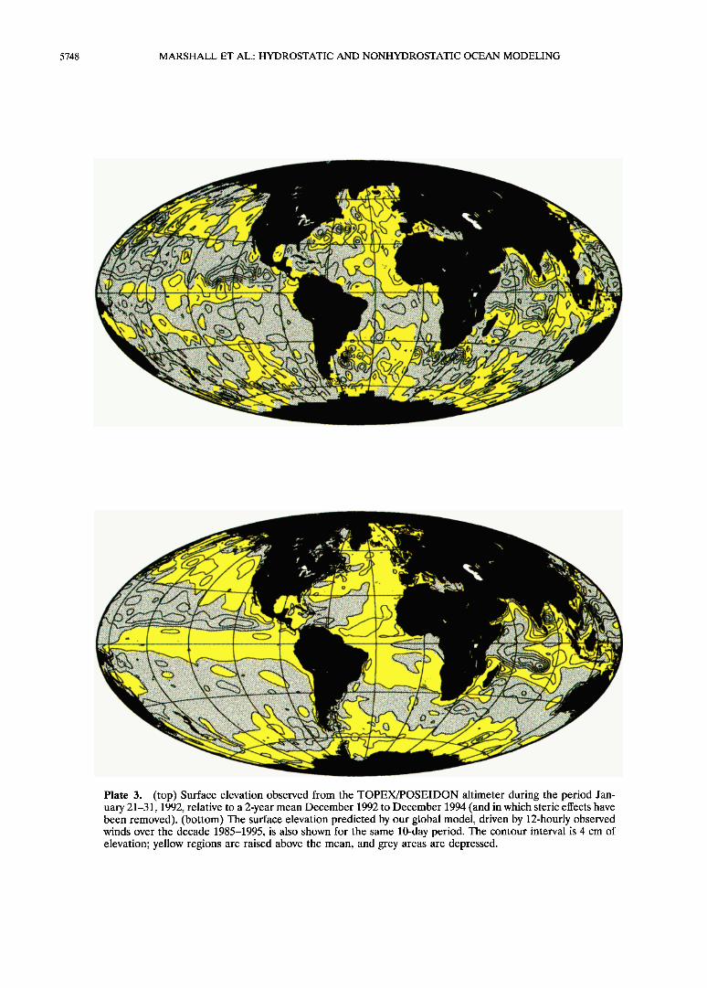
Figure 7 shows surface currents from our simulation using HPE; thus only a 2-D elliptic problem for the surface pressure was inverted. Plate 3 compares the surface elevation observed from the TOPEX/POSEIDON altimeter during the period January 21-31, 1992 (prepared by Detlef Stammer of MIT), to

the surface elevation predicted by the model for the same period. The broad agreement is very encouraging, demonstrat- ing not only that the model has fidelity in reproducing basin- scale variability induced by winds but also that the TOPEX/ POSEIDON altimeter provides us with a remarkable global data set for comparing with models and theory. Integrations of the model with NH instead of HPE, in which the vertical

velocity is obtained by prognostic integration of (43), instead of being diagnosed from continuity, give indistinguishable results in this limit where n --• 0; our chosen preconditioner is then an exact inverse of d2/dz 2 and solves the ODE in one application; see Table 2. Thus use of NH involves only marginally more computation than HPE.

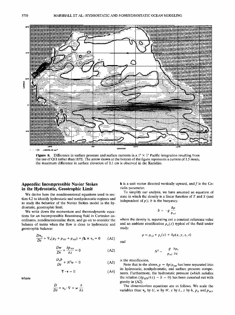
Figure 8 plots the difference in P s and surface currents obtained from Pacific integrations using HPE and QH at 1 ø horizontal resolution. Inclusion in QH of a full treatment of

the Coriolis force only leads to small differences in current speeds (---1-2 mm s -j) and surface elevation (---0.1 cm) at this resolution.

6. Conclusions

We have critically reviewed some of the key assumptions inherent in the hydrostatic primitive equations (HPEs) and described and implemented more accurate nonhydrostatic (NH) and quasi-hydrostatic (QH) formulations for studies of ocean circulation from convective to global scale.

Rather than assume hydrostatic balance a priori (the left- pointing arrow in Figure 1), we have retained the material derivative Dw/Dt in the vertical momentum equation and developed a model based on the incompressible Navier Stokes equations. Such models are designed primarily for the study of small-scale phenomena, such as mixed layer physics and convective processes in the laboratory and the ocean. The pressure field, which ensures that evolving currents remain nondivergent, is found by inversion of a three-dimensional elliptic operator, the overhead of the nonhydrostatic algorithm. A strategy has been outlined and illustrated which separates the pressure into its constituent parts: Ps, Pz•v, and PNH. As in HPE and QH a 2-D elliptic problem must be inverted for P s; but in NH, a further 3-D Poisson equation must be inverted for PNH. A preconditioner is designed which, in the hydrostatic limit, is an exact integral of the elliptic operator and so leads to an algorithm that seamlessly moves from nonhydrostatic to hydrostatic limits. Moreover, when employed in the hydrostatic limit, the nonhydrostatic model is fast, competitive with the fastest ocean climate models in use today based on the HPEs. It is thus ideal for the study of the whole range of phenomena presented in Figure 1 (the right-pointing arrow) and particularly those in the grey area. Our main conclusions are the following:

1. Ocean models based on consistent equation sets that are more accurate than the HPEs can be formulated and efficiently implemented: NH and OH.

2. Ocean models based on algorithms rooted in the incompressible Navier Stokes equations can be constructed which perform efficiently across the whole range of scales, from the convective to the global. Such models are endowed with great versatility; their nonhydrostatic capability renders them suitable for study of small-scale phenomenon. When deployed to study hydrostatic phenomena, they are no more demanding of


20 .• 20

lO

o 0 50 .• 0 10 20 30 40

Along channel distance (kin). 10 20 30 40

Along channel distance (km). 50

.

,•, 500

.• 1000

• 1500

2000

.

500

-•1ooo

•1500

2000 10 20 30 40

Along channel distance (kin). 50 0 10 20 30 40 50

Along channel distance (km).

Vertical velocity (m/s).

-0.15 -0.1 -0.05 0 0.05

0.05 o

-0.05

• -0.15 10 20 30 40 50

Along channel distance (kin).

0.05 "

o -0.05

-0.1 -0.15 ß

0 10 20 30 40 50 Along channel distance (km).

Plate 2. On the left the vertical velocity is plotted obtained by integration of NH at day 6 of the mixed layer channel calculation. On the right the same fields are plotted but obtained by integration of HPE. The bottom two panels compare w(x, y - 27 km, z - 400) from (left) NH and (right) HPE also at day 6.

computation than hydrostatic models. Moreover, algorithms rooted in NH may offer a number of advantages over those based on HPE.

3. In large-scale integrations (at 1 ø horizontal resolution), HPE, QH, and NH give essentially the same numerical solutions. The neglect of cos 0 Coriolis terms is the most questionable assumption made by the HPEs, but their inclusion (in QH and NH) yields differences in horizontal currents of only a few millimeters per second (in the rather coarse resolution

global experiment presented here). Thus it is clear that solutions based on the HPEs are not grossly in error at least at coarse resolution. Nevertheless, models based on QH (or NH) ought to be preferred.

Finally, we conclude by mentioning some future directions. In addition to the use of the model described here as a general- purpose tool for study of the ocean, one might anticipate that its nonhydrostatic capability would render it particularly suitable for hydrodynamical studies of mixed layers and coastal


Plate 3. (top) Surface elevation observed from the TOPEX/POSEIDON altimeter during the period Jan- uary 21-31, 1992, relative to a 2-year mean December 1992 to December 1994 (and in which steric effects have been removed). (bottom) The surface elevation predicted by our global model, driven by 12-hourly observed winds over the decade 1985-1995, is also shown for the same 10-day period. The contour interval is 4 cm of elevation; yellow regions are raised above the mean, and grey areas are depressed.


40øN

0 o

40øS

80øS O•øE 100øE 160øW

> 05 rn$ -• ß LONGITUDE

• lOøS [.•

20ø$

20øN

10øN

0 o

30ø8

40øS

80øE 100øE 120øE 140øE 160øE > 0.5 rrts -t LONGITUDE

60øW

Figure 7. Currents at a depth of 50 m in a numerical simulation of the global ocean using HPE on a 128-node CM5. The model, which has a horizontal resolution of 1 ø x 1 ø and 20 levels in the vertical, was driven by monthly-mean winds and climatological fluxes of heat and fresh water for a period of 40 years and initialized from the Levitus climatology. We show here the flow during the spring of the thirty-eighth year of integration. In the global map, every other current vector is plotted; the inset shows current vectors at the resolution of the model.

regions where nonhydrostatic processes play an important role. Height is used as a vertical coordinate by Marshall et al. [this issue]; terrain-following-coordinate, nonhydrostatic models could readily be implemented. Isopycnal nonhydrostatic forms would seem to have limited application; isopycnal coordinates are not naturally suited to the study of convective processes, for example. But nonhydrostatic height-coordinate models

could be used to represent upper ocean processes in conjunc- tion with hydrostatic models (perhaps formulated isopycnally) to represent the geostrophic interior of the ocean.

One of the avenues that the authors are actively pursuing is the construction of a sibling atmospheric model based on, as outlined by Brugge et al. [1991], the same hydrodynamical formulation as described here.


140øE 180' 140øW 1oo,w LONGITUDE

• t.50000g-03

Figure 8. Difference in surface pressure and surface currents in a 1 ø x 1 ø Pacific integration resulting from the use of QH rather than HPE. The arrow shown at the bottom of the figure represents a current of 1.5 mm/s; the maximum difference in surface elevation of 0.1 cm is observed in the Kurishio.

Appendix: Incompressible Navier Stokes in the Hydrostatic, Geostrophic Limit

We derive here the nondimensional equations used in section 4.2 to identify hydrostatic and nonhydrostatic regimes and to study the behavior of the Navier Stokes model in the hydrostatic, geostrophic limit.

We write down the momentum and thermodynamic equations for an incompressible Boussinesq fluid in Cartesian coordinates, nondimensionalize them, and go on to consider the balance of terms when the flow is close to hydrostatic and geostrophic balance:

OYh Ot + Vh(Ps + Pro. + Ps,) + fk x ¾h -- 0 (A1)

D w Op N H Dt + • = 0 (A2)

Dhb Ot -- + N2w = 0 (A3)

where

D

Dt

V.v = 0 (A4)

0

---Vh.V + W OZ

k is a unit vector directed vertically upward, and f is the Co- riolis parameter.

To simplify our analysis, we have assumed an equation of state in which the density is a linear function of T and S (and independent of p); b is the buoyancy:

8p

Pref

where the density is, separating out a constant reference value and an ambient stratification po(Z) typical of the fluid under study:

/9 -• Pref -'l- po(Z) d- ap(X, y, z, t)

and

5 2 -- g Opo

Pref 0 Z

is the stratification.

Note that in the above, p = t•p/Pref has been separated into its hydrostatic, nonhydrostatic, and surface pressure components. Furthermore, the hydrostatic pressure (which satisfies the relation (Opi_iy/Oz) - b = 0) has been canceled out with gravity in (A2).

The dimensionless equations are as follows. We scale the variables thus: % by U, w by W, x by L, z by h, Ps and p/_/y


by P/_/y, pN/_/ by PN/_/, f by F, b by # (p 1/Pref), and N 2 by (#/h)(APo /Pref), where p• is a measure of the magnitude of 8p(x, y, z) and Apo is the change in Po over a depth h.

Setting D/Dt -• (U/L) (D'/Dt'), etc., where the prime symbols indicate nondimensional parameters, (A1)-(A4) become

where

V;. v; + Ro Oz-•-= 0 (A4")

D'v• Dt' --+ V;(ps +pro,+ npm-/) + k x v• = 0

(Ai')

is the nonhydrostatic parameter identified in section 2.1 and used in section 4.2.

' PnY Op•vi• 0 (A2') • t -- Dt + n Oz

DID l

Dt' Pl / (A3')

where

V;. v; + Oz' 0

P NH

(A4')

is the nonhydrostatic parameter. Now let us suppose that the flow is close to geostrophic and

hydrostatic balance: geostrophic

hydrostatic

PHV FL 1 : (AS) U 2 - U Ro

plgh PH¾ = (A6)

JOref

Continuity (A4') together with geostrophy implies that

WL

U h Ro

and since (D'/Dt)b' • N'2w ' • 1, (A3') implies that

WL 91

U h A9o

(A7)

(A8)

Combining (A5), (A6), (A7), and (A8), we deduce that

R,Ro 2 = 1 (A9)

where R i is the Richardson number of the flow given by

N2h 2 gApoh c • R l = U2 -- /9refU •= U2 (A10)

and c is the speed of internal gravity waves. The result (A9) is well known and defines the quasi-

geostrophic regime; if R i of the large-scale flow is large, then the R o is small and the flow is quasi-geostrophic.

We may now write the set (Ai')-(A4') in terms of R i, R o, and 3, = h/L; the aspect ratio of the motion thus

D'v• 1

D + •oo [V;(pk + p•/r + npk,) + f'k x v;] = 0 (AI") D ' w' Op •vs

+ = 0 (A2") Dr' Oz'

D•D •

Dr' -- + N' 2w' = 0 (A3")

Acknowledgments. This study was supported by grants from ARPA, ONR, and TEPCO. The model was developed on the CM5 housed in the Laboratory for Computer Science (LCS) at MIT as part of the SCOUT initiative. Much advice and encouragement on computer science aspects of the project was given by Arvind of LCS. Jacob White of the Department of Electrical Engineering and Computer Science at MIT advised on the solution of elliptic problems on parallel domputers. We often consulted Andy White of the UK Meteorological Otfice and our colleague Jochem Marotzke on the mathematical and numerical formulation of the ocean model.

References

Adcroft, A., C. Hill, and J. Marshall, On the representation of topography using shaved cells in height coordinate ocean models, Mon. Weather Rev., in press, 1996.

Bretherton, F. P., Critical layer instability in baroclinic flows, Q. J. R. Meteorol. Soc., 92, 325-334, 1966.

Browning, G. L., W. R. Holland, H.-O. Kreiss, and S. J. Worley, An accurate hyperbolic system for approximately hydrostatic and incompressible flows, Dyn. Atmos. Oceans, 14, 303-332, 1990.

Brugge, R., H. L. Jones, and J. C. Marshall, Non-hydrostatic ocean modeling for studies of open-ocean deep convection, in Deep Con- vection and Deep Water Formation in the Oceans, Elsevier Oceanogr. Set., vol. 57, pp. 325-340, Elsevier Sci., New York, 1991.

Bryan, K., A numerical model for the study of the circulation of the world ocean, J. Cornput. Phys., 4, 347-376, 1969.

Dukowicz, J. K., and A. S. Dvinsky, Approximate factorization as a high order splitting for the implicit incompressible flow equations, J. Cornput. Phys., 102, 336-347, 1992.

Dukowicz, J. K., R. D. Smith, and R. C. Malone, A reformulation and implementation of the Bryan-Cox-Semtner ocean model on the con- nection machine, J. Atmos. Oceanic Technol., 10, 195-208, 1993.

Eckart, C., The Hydrodynamics of Oceans and Atmospheres, Pergamon, Tarrytown, N.Y., 1960.

Gill, A., Atmosphere-Ocean Dynamics, Academic, San Diego, Calif., 1982.

Gresho, P.M., and R. Sani, On pressure boundary conditions for the incompressible Navier-Stokes equations, Int. J. Numer. Methods Flu- ids, 7, 1111-1145, 1987.

Haine, T., and J. Marshall, Gravitational, symmetric and baroclinic instability of the oceanic mixed layer, J. Phys. Oceanogr., in press, 1996.

Harlow, F. H., and J. E. Welch, Time depended viscous flow, Phys. Fluids, 8, 2182-2193, 1965.

Jones, H., and J. Marshall, Convection with rotation in a neutral ocean: A study of open-ocean deep convection, J. Phys. Oceanogr., 23, 1009-1039, 1993.

Julien, K., S. Legg, J. McWilliams, and J. Werne, Rapidly rotating turbulent Raleigh-Benard convection, J. Fluid Mech., in press, 1996.

Klinger, B., J. Marshall, and U. Send, Representation of convective plumes by vertical adjustment, J. Geophys. Res., 101(C8), 18,175- 18,182, 1996.

Legg, S., and J. Marshall, A heton model of the spreading phase of open-ocean deep convection, J. Phys. Oceanogr., 23, 1041-1056, 1993.

Lorenz, E. N., The nature and theory of the general circulation of the atmosphere, WMO 218, TP 115, World Meteorol. Organ., Geneva, Switzerland, 1967.

Mahadevan, A., J. Oliger, and R. Street, A non-hydrostatic mesoscale ocean basin model, I, Well-posedness and scaling, J. Phys. Oceanogr., in press, 1996a.

Mahadevan, A., J. Oliger, and R. Street, A non-hydrostatic mesoscale


ocean model, II, Numerical implement•ition, J. Phys. Oceanogr., in press, 1996b.

Marshall, J., A. Adcroft, C. Hill, L. Perelman, and C. Heisey, A finite-volume, incompressible Navier Stokes model for studies of the ocean on parallel computers, J. Geophys. Res., this issue.

Miller, M. J., On the use of pressure as vertical coordinate in modeling convection, Q. J. R. Met•orol. Soc., 100, 155-162, 1974.

Miller, M. J., and A. A. White, On the non-hydrostatic equations in pressure and sigma coordinates, Q. J. R. Meteorol. Soc., 110, 515- 533, 1984.

Norbury, J., and M. J.P. Cullen, A note on the properties of the hydrostatic equations of motion, Q. J. R. Meteorol. Soc., 111, 1135- 1137, 1985.

Phillips, N. A., The equation of motion for a shallow rotating atmosphere and the 'traditional approximation,' J. Atmos. Sci., 23, 626- 628, 1966.

Phillips, N. A., Reply to G. Veronis's comments on Phillips (1966), J. Atmos. Phys., 23, 626-628, 1968.

Phillips, N. A., Principles of large-scale numerical weather prediction, in Dynamic Meteorology, edited by P. Morel, pp. 1-96, D. Reidel, Norwell, Mass., 1973.

Potter, D., Computational Physics, John Wiley, New York, 1976. Veronis, G., Comments on Phillips's (1966) proposed simplification of

the equation of motion for a shallow rotating atmosphere, J. Atmos. Sci., 25, 1154-1155, 1968.

Wangsness, R. K., Comments on "The equation of motion for a shallow rotating atmosphere and the 'traditional approximation,'" J. Atmos. Sci., 27, 504-506, 1970.

White, A. A., and R. A. Bromley, Dynamically consistent, quasi- hydrostatic equations for global models with a complete representation of the Coriolis foice, Q. J. R. Meteorol. Soc., 121, 399-418, i995.

Whitehead, J. A., J. Marshall, and G. Hufford, Localized convection in rotating stratified fluid, J. Geophys. Res., 101(Cll), 25,705-25,721, t996.

Williams, G. P., Numerical integration of the three-dimensional Navier Stokes equations for incompressible flow, J. Fluid 'Mech., 37, 727-750, 1969.

A. Adcroft, C. Hill, J. Marshall, and L. Perelman, Center for Me- teorology and Physical Oceanography, Department of Earth, Atmo- spheric and Planetary Sciences, Massachusetts Institu te of TechnOlo•, Building 54, Room 1526, Cambridge, MA 02139. (e-mail: marshall@gulf. mit.edu)

(Received August 31, 1995; revised July 31, 1996; accepted August 21, 1996.)

Date post:	30-Apr-2020
Category:	Documents
Upload:	others
View:	73 times
Download:	1 times

Hydrostatic, quasi-hydrostatic, and nonhydrostatic ocean...

Documents