Principles of Statistics Assoc. Prof. Dr. Abdul Hamid b. Hj. Mar Iman Former Director, Centre for Real Estate Studies Faculty of Geoinformation Science and Engineering, Universiti Teknologi Malaysia, Skudai, Johor. E-mail: [email protected]. Hypothesis Testing. Content: - PowerPoint PPT Presentation
Principles of Statistics Assoc. Prof. Dr. Abdul Hamid b. Hj. Mar Iman Former Director, Centre for Real Estate Studies Faculty of Geoinformation Science and Engineering, Universiti Teknologi Malaysia, Skudai, Johor. E-mail: [email protected]
Transcript
Principles of Statistics
Assoc. Prof. Dr. Abdul Hamid b. Hj. Mar ImanFormer Director,
Centre for Real Estate StudiesFaculty of Geoinformation Science and Engineering,
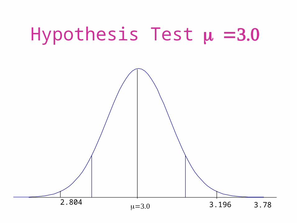
The null hypothesis that the mean is equal to 3.0:
Example
You suspect that the mean rental of 225 purpose-built office units in Johor is RM 3.00/sq.ft. If the std. dev. is RM 1.50/sq.ft., what is the 95% confidence interval of the mean?
The alternative hypothesis that the mean does not equal to 3.0:
Ho: μ = 3.0
H1: μ 3.0
x
A Sampling Distribution
-XL = ? XU = ?
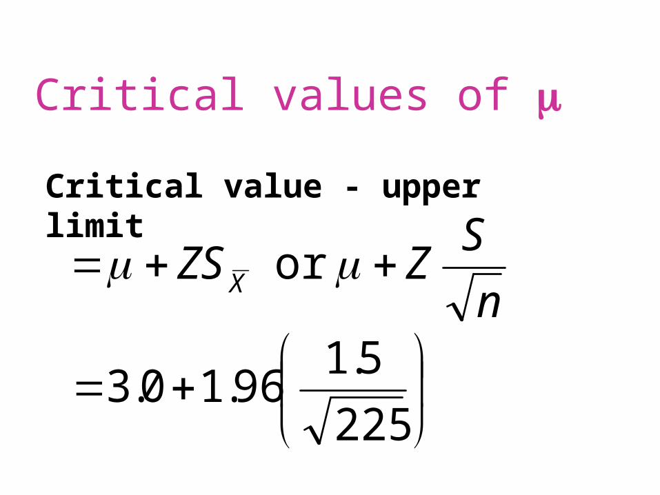
Critical values of
Critical value - upper limit
n
SZZS X or
225
5.196.1 0.3
1.096.1 0.3
196. 0.3
196.3
Critical values of
Critical value - lower limit
n
SZZS
X- or -
225
5.196.1- 0.3
Critical values of
1.096.1 0.3
196. 0.3
804.2
Critical values of
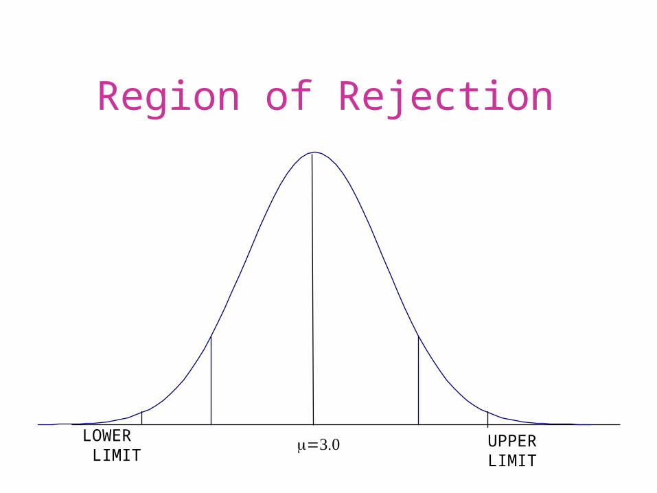
Region of Rejection
LOWER LIMIT
UPPERLIMIT
Hypothesis Test
2.804 3.196 3.78
Accept null Reject null
Null is true
Null is false
Correct-Correct-no errorno error
Type IType Ierrorerror
Type IIType IIerrorerror
Correct-Correct-no errorno error
Type I and Type II Errors
Type I and Type II Errorsin Hypothesis Testing
State of Null Hypothesis Decisionin the Population Accept Ho Reject Ho
Ho is true Correct--no error Type I errorHo is false Type II error Correct--no error
Example
You estimate that the average price, μ, of single-
and double-storey houses in Malaysia’s major
industrialised towns to be RM 1,600/sq.m.
Based on a sample of 101 houses, you found
that the mean price, , is 1,579.44/sq.m. with a std
dev. of RM 350.13/sq.m.
(a) Would you reject your initial estimate at 0.05 significance level?
(b) What is the confidence interval of rental at 5% s.l.?
Since Z < Zc,do not reject Ho. ∴ Rental = RM 1,600/sq.m.
Answer (b)
1,579.13-1.645(34.84)=RM 1,521.82 (lower limit)
1,579.13+1.645(34.84)=RM 1,636.44 (upper limit)
PARAMETRICSTATISTICS
NONPARAMETRICSTATISTICS
t-Distribution
• Symmetrical, bell-shaped distribution
• Mean of zero and a unit standard deviation
• Shape influenced by degrees of freedom
Degrees of Freedom
• Abbreviated d.f.
• Number of observations
• Number of constraints
or
Xlc StX ..
n
StX lc ..limitUpper
n
StX lc ..limitLower
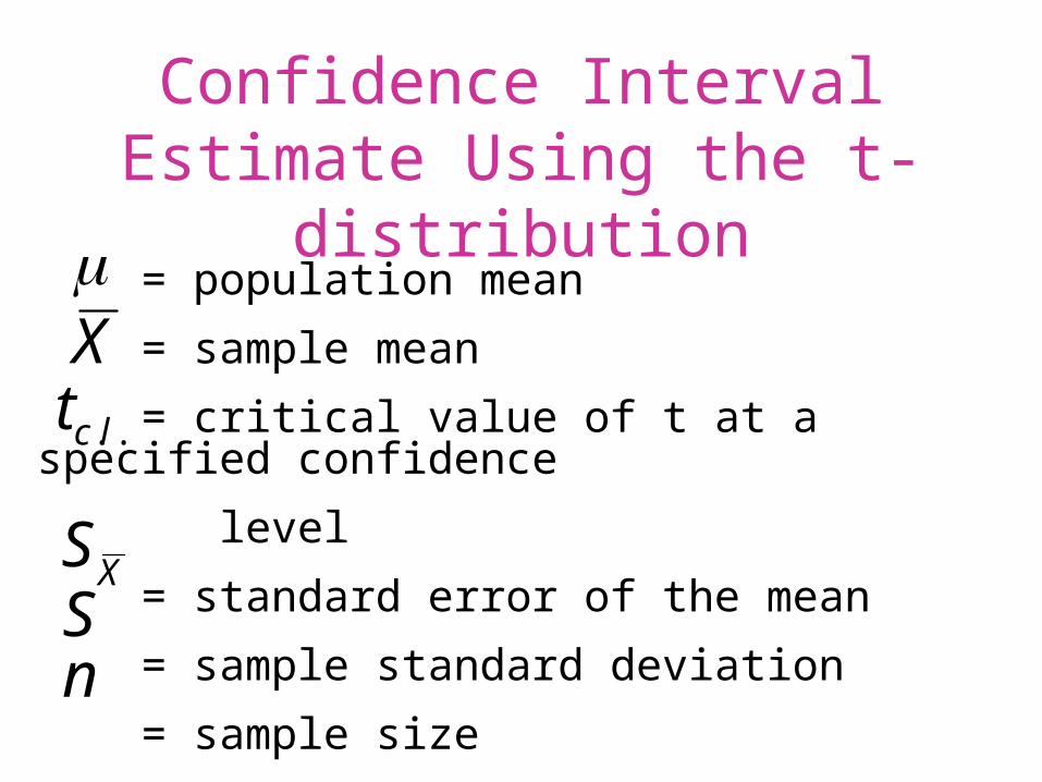
Confidence Interval Estimate Using the t-distribution
= population mean
= sample mean
= critical value of t at a specified confidence
level
= standard error of the mean
= sample standard deviation
= sample size
..lct
X
XSSn
Confidence Interval Estimate Using the t-distribution
xcl stX
17
66.2
7.3
n
S
X
Confidence Interval Estimate Using the t-distribution
07.5
)1766.2(12.27.3limitupper
33.2
)1766.2(12.27.3limitLower
Hypothesis Test Using the t-Distribution
Suppose that a production manager believes the average number of defective assemblies each day to be 20. The factory records the number of defective assemblies for each of the 25 days it was opened in a given month. The mean was calculated to be 22, and the standard deviation, ,to be 5.
XS
Univariate Hypothesis Test Utilizing the t-Distribution
20 :
20 :
1
0
H
H
nSS X /25/5
1
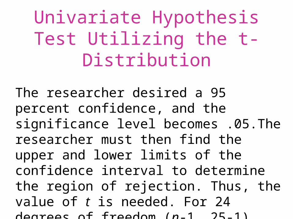
The researcher desired a 95 percent confidence, and the significance level becomes .05.The researcher must then find the upper and lower limits of the confidence interval to determine the region of rejection. Thus, the value of t is needed. For 24 degrees of freedom (n-1, 25-1), the t-value is 2.064.
Univariate Hypothesis Test Utilizing the t-Distribution
:limitLower 25/5064.220 .. Xlc St 1064.220
936.17
:limitUpper 25/5064.220 ..
Xlc St 1064.220
064.20
X
obs S
Xt
1
2022
1
2
2
Univariate Hypothesis Test t-Test
Testing a Hypothesis about a Distribution
• Chi-Square test
• Test for significance in the analysis of frequency distributions
• Compare observed frequencies with expected frequencies
• “Goodness of Fit”
i
ii )²( ²
E
EOx
Chi-Square Test
x² = chi-square statisticsOi = observed frequency in the ith cellEi = expected frequency on the ith cell
Chi-Square Test
n
CRE ji
ij
Chi-Square Test Estimation for Expected Number
for Each Cell
Chi-Square Test Estimation for Expected Number
for Each Cell
Ri = total observed frequency in the ith rowCj = total observed frequency in the jth columnn = sample size
2
222
1
2112
E
EO
E
EOX
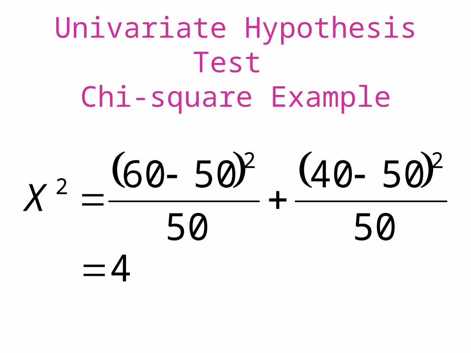
Univariate Hypothesis Test Chi-square Example
50
5040
50
5060 222
X
4
Univariate Hypothesis Test Chi-square Example
Hypothesis Test of a Proportion
is the population proportion
p is the sample proportion
is estimated with p
5. :H
5. :H
1
0
Hypothesis Test of a Proportion
100
4.06.0pS
100
24.
0024. 04899.
pS
pZobs
04899.
5.6.
04899.
1. 04.2
0115.Sp
000133.Sp 1200
16.Sp
1200
)8)(.2(.Sp
n
pqSp
20.p 200,1n
Hypothesis Test of a Proportion: Another Example
0115.Sp
000133.Sp 1200
16.Sp
1200
)8)(.2(.Sp
n
pqSp
20.p 200,1n
Hypothesis Test of a Proportion: Another Example
Indeed .001 the beyond t significant is it
level. .05 the at rejected be should hypothesis null the so 1.96, exceeds value Z The