Hysteresis Behavior Patterns in Complex Systems A Thesis Submitted to the Faculty of Drexel University by Ondrej Hovorka in partial fulfillment of the requirements for the degree of Doctor of Philosophy August 2007 brought to you by CORE View metadata, citation and similar papers at core.ac.uk provided by Drexel Libraries E-Repository and Archives
Transcript
Hysteresis Behavior Patterns in Complex Systems
A Thesis
Submitted to the Faculty
of
Drexel University
by
Ondrej Hovorka
in partial fulfillment of the
requirements for the degree
of
Doctor of Philosophy
August 2007
brought to you by COREView metadata, citation and similar papers at core.ac.uk
provided by Drexel Libraries E-Repository and Archives
First, I would like to thank my advisor, Prof. Gary Friedman, for educating me,for giving me so much freedom, for all those interesting discussions, and for beingso supportive in every imaginable respect. It is hard to express how lucky I am towork with him, and generally, to know him. I would also like to express my thanks toDr. Andreas Berger, collaboration with whom was, and continues to be, a fantasticeducational experience.
I am grateful to all my PhD committee members: Prof. Adam Fontecchio, Prof.Jaudelice Cavalcante de Oliveira, Prof. Nagarajan Kandasamy, and Prof. Alexan-der Fridman for their encouragement and for useful suggestions to improve this thesis.
I have spent long hours discussing scientific, philosophical, and other kinds of ques-tions with my friends Roman Groger, Ben Yellen, Hemang Shah, Ruchita Vora,Vasileios Nasis, Greg Fridman, Kara Heinz, Halim Ayan, Eda Yildirim, Alex Chi-rokov, Alex Fridman, Anna Fox, Derek Halverson, Dave Delaine, Kashma Rai, SameerKalghatgi, William Norman, Mike Warde, Pavol Pcola, Ivan Oprencak, and manyothers. Each of them played part in composing this thesis.
I want to thank my wife Veronika, for her love, for taking care of everything neededto be taken care of, for her unbelievable patience, and generally, for being my wife.Many thanks go to all my family for their support, and to my brother Michal whoserves me as an example.
2.1 Linear RC circuit and the (non-hysteretic) dependence of the outputvoltage V0 across the capacitor on the input voltage Vi. Elliptic loop isdue to the phase shift between the input and output and its size andorientation depends on the frequency. . . . . . . . . . . . . . . . . . . 6
2.2 Origins of hysteresis. (a) The free energy landscape as a function ofstate variable M for two different values of the external parameter H.As H changes, the energy landscape becomes distorted and transitionsbetween different states become possible. (b) Due to very short timescale, the transition between different states appears as being sharp ifplotted in the state vs. external parameter plane. When the externalparameter returns to the original value Ha, the state variable does not,and hysteresis is displayed. . . . . . . . . . . . . . . . . . . . . . . . . 8
2.3 Minor cycle types. (a) Major hysteresis loop with two minor loopsinside. Minor loops 1 and 2 correspond to the same reversal fields.(b) Closed loops: C-type cycles, (c) Tilting cycles: T -type cycles, (d)Cycles with subharmonic period: S-type cycles, (e) Drifting cycles;Reptation: R-type cycles. . . . . . . . . . . . . . . . . . . . . . . . . 11
3.1 Preisach model. (a) Rectangular hysteresis loop of a relay - the basicbuilding block of the Preisach model. Each relay with thresholds αand β corresponds to a point in the Preisach plane (b). The staircaseinterface line L separates regions with positively and negatively flippedrelays, and its shape depends on the history of the applied field. . . . 17
3.2 Wiping out and congruency properties of the Preisach model. (a) Twominor loops with the same reversal points 1 and 2 corresponding todifferent field histories. (b-d) Evolution of state on the Preisach planeduring generation of a minor loop attached to the major hysteresis.(e-f) Generation of a minor loop with the same reversal fields obtainedafter first reversing the field at the point 3 on the major loop. . . . . 19
3.3 Examples of various graph structures: (a) Trees of the order k = 6.A linear chain of spins can be represented by a tree like graphs. (b)Cycle of order k = 6. The square lattice contains cycles of differentorders starting from k = 4. (c) Complete subgraphs of order k = 3, 4, 5. 25
3.4 Erdos-Renyi random network having 12 nodes and 11 edges. . . . . . 26
viii
3.5 Evolution of a graph structure. Different topological elements appearsuddenly at specific probabilities p. . . . . . . . . . . . . . . . . . . . 28
4.1 (a) Rectangular hysteresis loop corresponding to the switch si withsymmetric thresholds αi and βi = −αi, shifted from the coordinateorigin due to the interaction with the neighboring spins. (b) Whenthe interaction is equal to zero, all spins with symmetric thresholdslie in the Preisach plane on the line perpendicular to β = α line. Fornonzero interactions, both thresholds are shifted by an amount ∆i,which depends on the interaction strength and on the state of theneighbors of the spin si. . . . . . . . . . . . . . . . . . . . . . . . . . 31
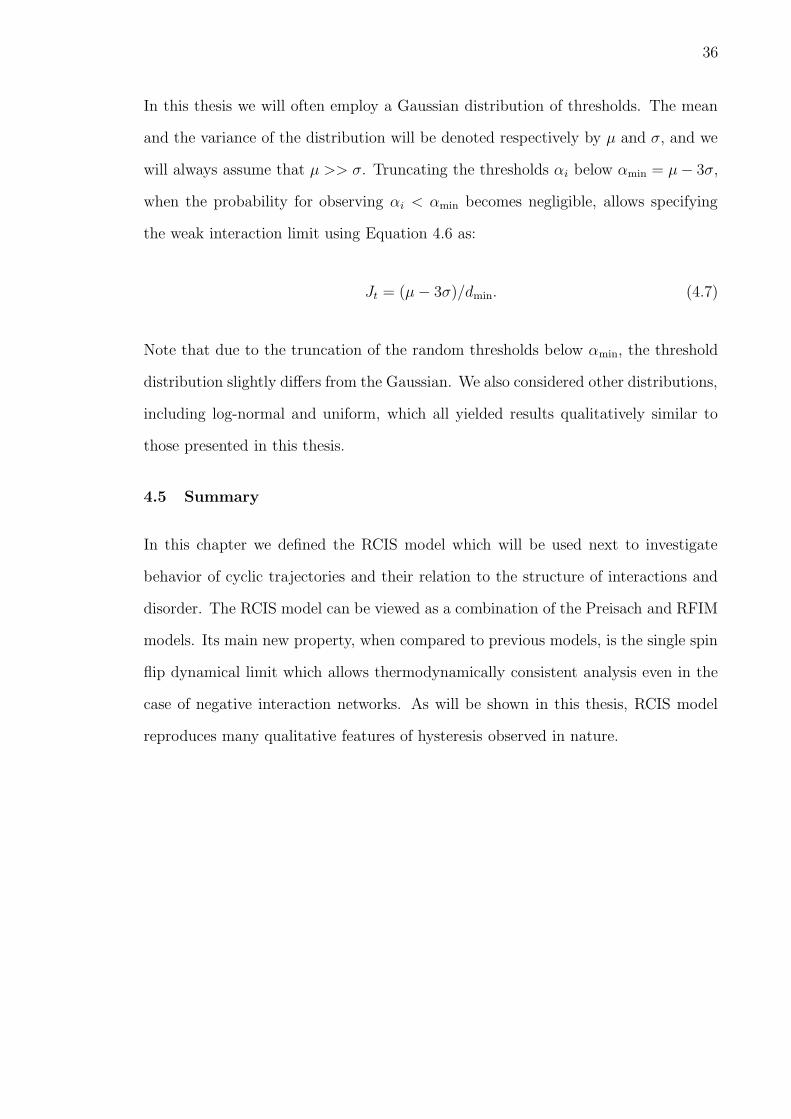
5.1 A(a-b) Minor loop cycled 3 times showing complete closure at the endof the first cycle for interaction weaker than the critical point. B(a-b) 3minor cycles showing opening for interaction stronger than the criticalpoint. . . . . . . . . . . . . . . . . . . . . . . . . . . . . . . . . . . . 38
5.2 Neel’s lattice. Shown are two interpenetrating lattices A and B (whiteand black dots) of spins. Magnetizations of each sub-lattice are Ma andMb. Spins do not interact within the sub-lattice. Interaction is onlybetween the spins from different lattices via the mean fields −J ′Ma
and −J ′Mb, where J ′ is the interaction magnitude. Magnetization ofthe entire system is an average M = (Ma +Mb)/2. . . . . . . . . . . 42
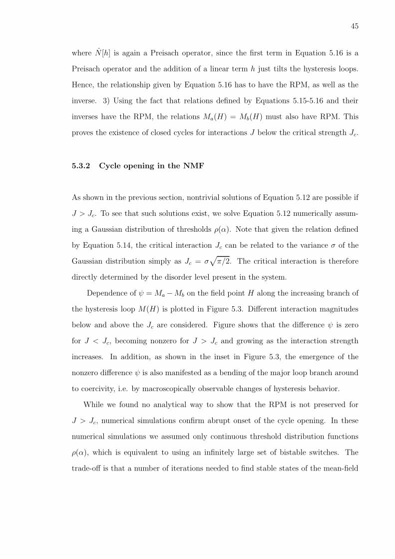
5.3 Difference ψ = Ma − Mb versus the external field H along the in-creasing major hysteresis loop branch (Hc is the coercive field whereM = 0). ψ = 0 for J < Jc and ψ 6= 0 for J > Jc. The maximumdifference appears around the coercive field. The results correspondto the Gaussian distribution of thresholds with variance σ = 1, whenJc = (π/2)1/2. The inset shows a change of shape of major hysteresisloop for J > Jc when ψ 6= 0. . . . . . . . . . . . . . . . . . . . . . . . 46
5.4 A sequence of cycle openings |∆M | numerically calculated for Neel’smean-field RCIS with a Gaussian distribution of thresholds (σ = 1,µ = 4). Interaction strengths are: a) J = 1.04Jc, b) J = 1.2Jc. . . . . 47
6.1 The opening region Ωo (top) and the extent of the cycle opening Λo
(bottom) as a function of normalized interaction strength for, respec-tively, the 2D nearest neighbor RCIS and the Neel’s mean field RCISmodels. The system size considered was 1600 spins and the data for thenearest neighbor model was averaged over 20 different random thresh-old realizations (Gaussian distribution with variance σ = 1, mean µ = 4). 50
ix
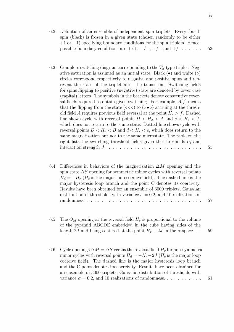
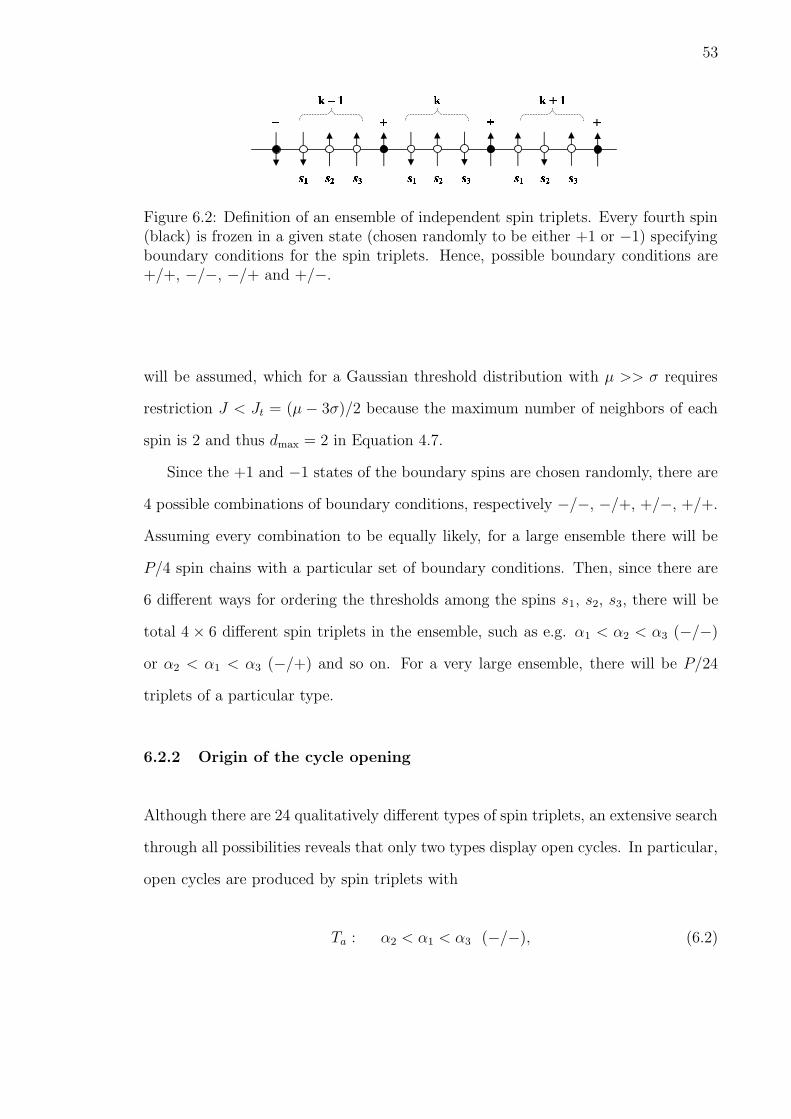
6.2 Definition of an ensemble of independent spin triplets. Every fourthspin (black) is frozen in a given state (chosen randomly to be either+1 or −1) specifying boundary conditions for the spin triplets. Hence,possible boundary conditions are +/+, −/−, −/+ and +/−. . . . . . 53
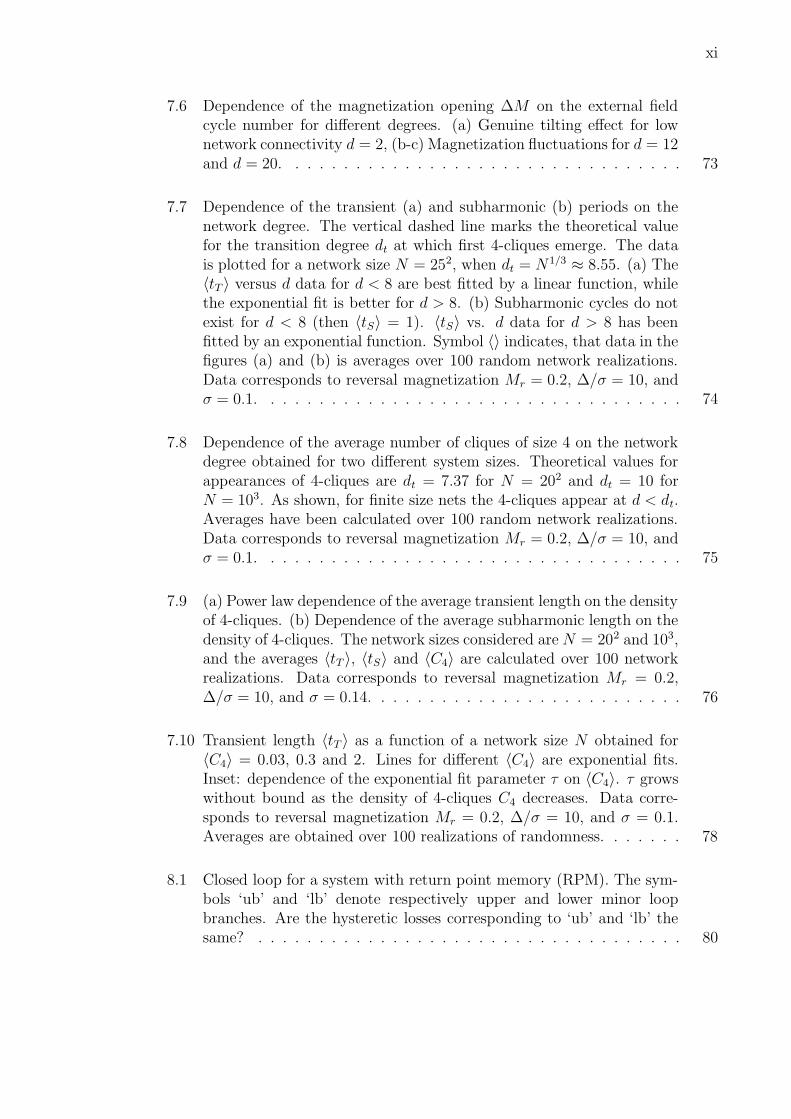
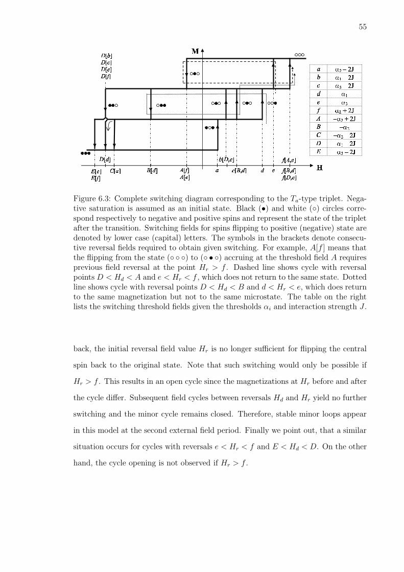
6.3 Complete switching diagram corresponding to the Ta-type triplet. Neg-ative saturation is assumed as an initial state. Black (•) and white ()circles correspond respectively to negative and positive spins and rep-resent the state of the triplet after the transition. Switching fieldsfor spins flipping to positive (negative) state are denoted by lower case(capital) letters. The symbols in the brackets denote consecutive rever-sal fields required to obtain given switching. For example, A[f ] meansthat the flipping from the state () to (•) accruing at the thresh-old field A requires previous field reversal at the point Hr > f . Dashedline shows cycle with reversal points D < Hd < A and e < Hr < f ,which does not return to the same state. Dotted line shows cycle withreversal points D < Hd < B and d < Hr < e, which does return to thesame magnetization but not to the same microstate. The table on theright lists the switching threshold fields given the thresholds αi andinteraction strength J . . . . . . . . . . . . . . . . . . . . . . . . . . . 55
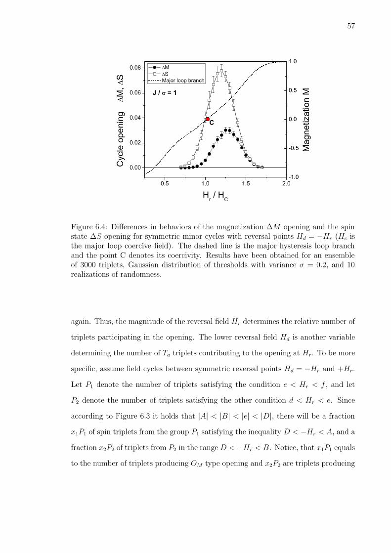
6.4 Differences in behaviors of the magnetization ∆M opening and thespin state ∆S opening for symmetric minor cycles with reversal pointsHd = −Hr (Hc is the major loop coercive field). The dashed line is themajor hysteresis loop branch and the point C denotes its coercivity.Results have been obtained for an ensemble of 3000 triplets, Gaussiandistribution of thresholds with variance σ = 0.2, and 10 realizations ofrandomness. . . . . . . . . . . . . . . . . . . . . . . . . . . . . . . . . 57
6.5 The OM opening at the reversal field Hr is proportional to the volumeof the pyramid ABCDE embedded in the cube having sides of thelength 2J and being centered at the point Hr − 2J in the α-space. . . 59
6.6 Cycle openings ∆M = ∆S versus the reversal fieldHr for non-symmetricminor cycles with reversal points Hd = −Hr+2J (Hc is the major loopcoercive field). The dashed line is the major hysteresis loop branchand the C point denotes its coercivity. Results have been obtained foran ensemble of 3000 triplets, Gaussian distribution of thresholds withvariance σ = 0.2, and 10 realizations of randomness. . . . . . . . . . . 61
x
6.7 Dependence of the maximum opening ∆M = ∆S on the interactionstrength for two different disorder magnitudes. Results were obtainedby using Equation 6.5, for Gaussian distribution ρ with mean µ >> σ.The cycle opening saturates for J >> σ reaching the universal constant1/18, and the approach to saturation is faster (i.e. lower interactionsare needed) for smaller disorder σ. . . . . . . . . . . . . . . . . . . . . 62
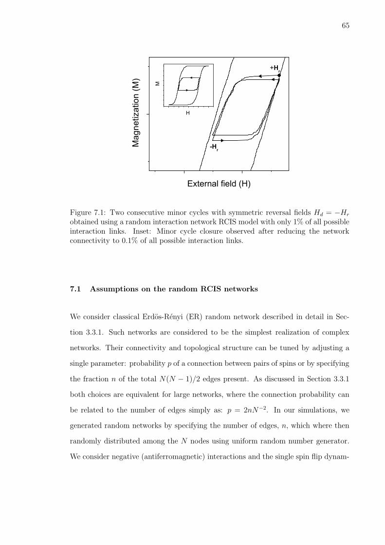
7.1 Two consecutive minor cycles with symmetric reversal fields Hd =−Hr obtained using a random interaction network RCIS model withonly 1% of all possible interaction links. Inset: Minor cycle closureobserved after reducing the network connectivity to 0.1% of all possibleinteraction links. . . . . . . . . . . . . . . . . . . . . . . . . . . . . . 65
7.2 Percent difference ∆S between the microstates before and after thefirst minor cycle plotted for different degrees d of the interaction net-work. Only symmetric reversals with Hd = −Hr are assumed, and Hr
corresponding to the magnetization Mr = 0.2, where the effect is thestrongest. Results are plotted for two system sizes N = 103 and 502
and the interaction energies ∆ = 1σ and ∆ = 10σ (σ is the variance ofthe Gaussian threshold distribution). Error-bars are about 1%. Inset:∆S versus d for N = 100 showing that ∆S = 0 for d = N . Error barsare about 4%. . . . . . . . . . . . . . . . . . . . . . . . . . . . . . . . 67
7.3 Dependence of the opening ∆S on the cycle number for different net-work degrees. For d = 2 and for d = 12 cycles converge within 4and 50 cycles respectively. For d > 13 the cycle convergence becomesvery slow as shown here for d = 20 and 100. The data is for 502 spinnetwork and averaged over 50 random graph and disorder realizations.Error-bar level is about 1%. Data correspond to reversal magnetizationMr = 0.2, ∆/σ = 10, and σ = 0.1. . . . . . . . . . . . . . . . . . . . . 69
7.4 Contour maps showing the cycle opening ∆S for different values of theinteraction energy ∆/σ and the network degree d (note the logarithmicscale of ∆/σ and d axes) for respectively: (a) 1-st, (b) 10-th, (c) 50-th,and (d) 100-th cycle. The lower bounds for the ‘limiting’ region withnon-converging cycles correspond to (∆/σ)t = 2.3 and dt ≈ 13. Dataare for N = 502, σ = 0.1 and averaged over 50 random graph anddisorder realizations. Error bars level is about 1%. . . . . . . . . . . . 70
7.5 Definition of the transient tT time and the subharmonic period tS.The steady state cycles reached after initial transient time tT ≥ 1 cancontain simple minor loops with tS = 1 or subharmonic cycles withtS > 1. Plot has been obtained for network with d = 20 and N = 103. 71
xi
7.6 Dependence of the magnetization opening ∆M on the external fieldcycle number for different degrees. (a) Genuine tilting effect for lownetwork connectivity d = 2, (b-c) Magnetization fluctuations for d = 12and d = 20. . . . . . . . . . . . . . . . . . . . . . . . . . . . . . . . . 73
7.7 Dependence of the transient (a) and subharmonic (b) periods on thenetwork degree. The vertical dashed line marks the theoretical valuefor the transition degree dt at which first 4-cliques emerge. The datais plotted for a network size N = 252, when dt = N1/3 ≈ 8.55. (a) The〈tT 〉 versus d data for d < 8 are best fitted by a linear function, whilethe exponential fit is better for d > 8. (b) Subharmonic cycles do notexist for d < 8 (then 〈tS〉 = 1). 〈tS〉 vs. d data for d > 8 has beenfitted by an exponential function. Symbol 〈〉 indicates, that data in thefigures (a) and (b) is averages over 100 random network realizations.Data corresponds to reversal magnetization Mr = 0.2, ∆/σ = 10, andσ = 0.1. . . . . . . . . . . . . . . . . . . . . . . . . . . . . . . . . . . 74
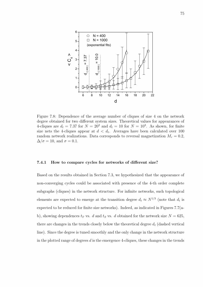
7.8 Dependence of the average number of cliques of size 4 on the networkdegree obtained for two different system sizes. Theoretical values forappearances of 4-cliques are dt = 7.37 for N = 202 and dt = 10 forN = 103. As shown, for finite size nets the 4-cliques appear at d < dt.Averages have been calculated over 100 random network realizations.Data corresponds to reversal magnetization Mr = 0.2, ∆/σ = 10, andσ = 0.1. . . . . . . . . . . . . . . . . . . . . . . . . . . . . . . . . . . 75
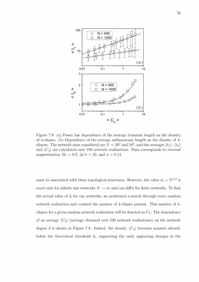
7.9 (a) Power law dependence of the average transient length on the densityof 4-cliques. (b) Dependence of the average subharmonic length on thedensity of 4-cliques. The network sizes considered are N = 202 and 103,and the averages 〈tT 〉, 〈tS〉 and 〈C4〉 are calculated over 100 networkrealizations. Data corresponds to reversal magnetization Mr = 0.2,∆/σ = 10, and σ = 0.14. . . . . . . . . . . . . . . . . . . . . . . . . . 76
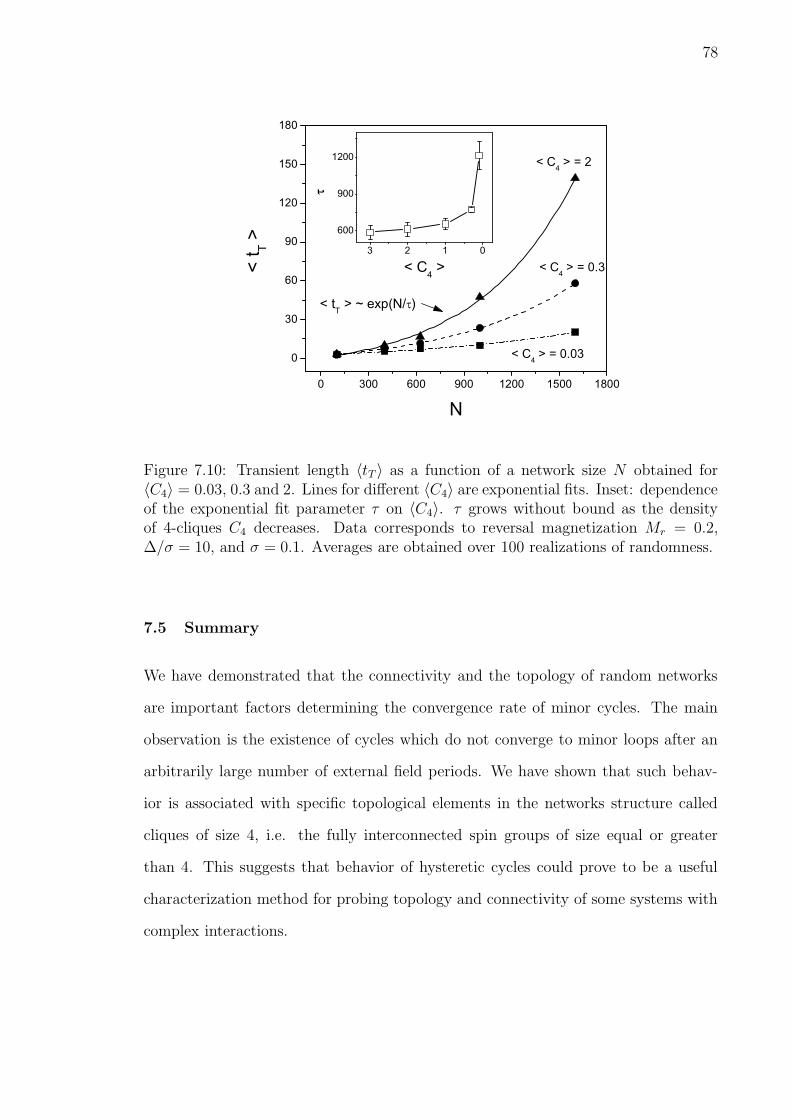
7.10 Transient length 〈tT 〉 as a function of a network size N obtained for〈C4〉 = 0.03, 0.3 and 2. Lines for different 〈C4〉 are exponential fits.Inset: dependence of the exponential fit parameter τ on 〈C4〉. τ growswithout bound as the density of 4-cliques C4 decreases. Data corre-sponds to reversal magnetization Mr = 0.2, ∆/σ = 10, and σ = 0.1.Averages are obtained over 100 realizations of randomness. . . . . . . 78
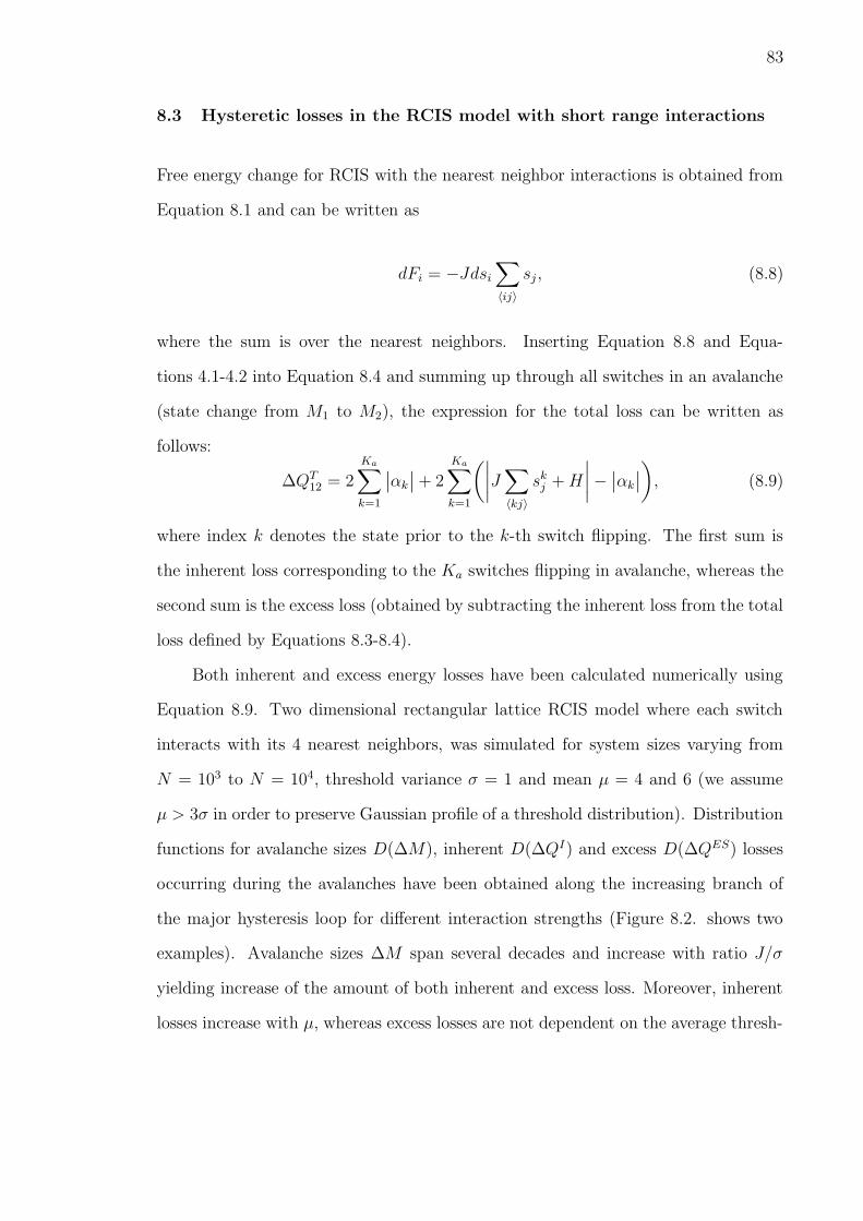
8.1 Closed loop for a system with return point memory (RPM). The sym-bols ‘ub’ and ‘lb’ denote respectively upper and lower minor loopbranches. Are the hysteretic losses corresponding to ‘ub’ and ‘lb’ thesame? . . . . . . . . . . . . . . . . . . . . . . . . . . . . . . . . . . . 80
xii
8.2 Distribution functions D for avalanches ∆M , inherent losses ∆QI , andexcess losses QES generated for 2 dimensional 40× 40 spin RCIS withσ = 1 and σ = 4 and 6 (Gaussian distribution of thresholds) and 100realizations of disorder. (a) J = 0.5, (b) J = 1.0. . . . . . . . . . . . . 84
8.3 Difference between hysteretic losses generated during the upper andlower minor loop branches for different reversal points Mr(Hr) on themajor hysteresis loop. Only minor loops with symmetric reversal pointsHd = −Hr are assumed. The data was averaged over 20 realizationsof randomness. The dashed line denotes a zero loss difference obtainedfor the mean field RCIS model. . . . . . . . . . . . . . . . . . . . . . 85
8.4 Difference between hysteretic losses for upper and lower minor loopbranches vs. the interaction strength. Data was averaged over 20realizations of randomness. Dashed line denotes a zero loss differenceobtained for the mean field RCIS model. . . . . . . . . . . . . . . . . 86
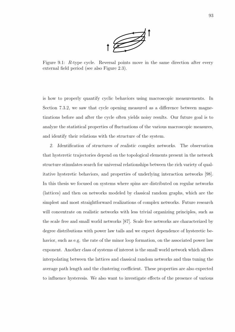
9.1 R-type cycle. Reversal points move in the same direction after everyexternal field period (see also Figure 2.3). . . . . . . . . . . . . . . . . 93
xiii
Abstract
Hysteresis Behavior Patterns in Complex SystemsOndrej Hovorka
Gary Friedman, Ph.D.
Many complex systems such as magnets, shape memory alloys, as well as socioe-
conomic and biological systems are known to display hysteresis. This inherently
irreversible process differs from the other irreversible processes most often addressed
in literature by the memory that persists long after the external parameters stop
changing. In general, hysteresis is a consequence of multi-scale system dynamics and
the existence of many metastable states. Although hysteresis is typically illustrated
by closed minor loops, other types of hysteretic trajectories are often observed where
closed loops form gradually after several external parameter periods or not at all.
The question arises: What in the structure of a system determines these qualitatively
different behaviors of hysteretic trajectories?
This thesis models complex hysteretic systems using a network of bistable binary
elements and investigates network structure induced changes in hysteretic behav-
ior. The main focus is on studying the minor loop formation processes for a single
cyclically varying external parameter. Stable minor loops are observed to form at
different rates as a function of the number of cycles, depending on the sign of the
interactions, disorder level, and on the connectivity and topology of the interaction
networks. For certain dense interaction networks, hysteretic trajectories that do not
converge to a minor loop after an arbitrarily large number of external parameter pe-
riods are discovered. It is shown that their appearance is related to the presence of
specific topological structures in the network. Thus, the thesis demonstrates several
interesting links between hysteretic behavior and the underlying structure of complex
systems.
1
Chapter 1. Scope of the thesis
This thesis describes analysis of a class of complex systems with hysteresis, which can
be viewed as networks of interacting bistable elements. Typically, the term ‘complex
system’ refers to a system consisting of many similar components, the interactions
between which create behavior that cannot be associated with the individual com-
ponents themselves. Such behavior is often called emergent. Several different types
of emergent properties have been investigated for various types of complex systems.
Among these properties are self-similarity in geometrical patterns and patterns in dy-
namic processes, such as power law scaling in the frequency spectrum of the system’s
evolution. Hysteresis is another example of emergent behavior. It can be defined
as any relationship between the state of the system and external parameters, which
depends on the history of the external parameter variation, but not on the rate of
this variation. Hysteresis is observed in many systems such as magnets, type-II su-
perconductors, shape memory alloys, as well as socioeconomic and biological systems.
This inherently irreversible process is a consequence of existence of many metastable
states and of multi-scale system dynamics.
Several interesting and widely observed features of hysteretic processes such as
power laws in the avalanche statistics have been investigated before. This thesis
focuses on the behavior of hysteretic processes in response to periodic variations of
external conditions whenever these can be described by a single real valued variable.
In part, this work is motivated by classical studies of cyclical behavior in non-linear
dynamic systems where response to periodic variations of the external variables is
known to be closely related to the structure of the system. Although hysteretic
systems can be viewed as a particular case of non-linear dynamic systems, cyclic
hysteretic processes have not been widely studied. As a result, hysteresis is typically
2
illustrated by closed loops in response to a periodic variation of an external parameter.
However, many other types of hysteretic trajectories can be observed where closed
loops form either gradually after several periods or not at all. Using a network
of interacting binary elements as a model, it is shown in this thesis that behavior
of hysteretic cycles is closely related to the sign of the interactions, their strength
relative to an inherent fixed disorder in the system, and to the network structure.
More specifically, it will be shown that positive interactions result in the return
point memory (RPM) property responsible for the recovery of system’s original in-
ternal state after every external parameter period, and leading to the formation of
closed minor loops at the end of the very first period. While such closed cycles are
also observed for some networks with negative interactions, it generally takes several
external parameter periods before a steady state with stable minor loops is reached.
It will be shown that the convergence to the steady state depends significantly on
the magnitude of interactions and on their topological structure. In addition, we
demonstrate the possibility of behavior not observed in binary networks previously,
where cycles become non-convergent and never form stable minor loops. Such non-
convergent cycles are shown to be associated with specific topological elements in the
network structure, suggesting that hysteretic trajectories can yield information about
the inherent structure of the complex systems.
The thesis is organized as follows. In Chapter 1 we introduce basic hysteresis
terminology and describe various types of hysteresis behaviors observed in systems
of different nature. In Chapter 2, most widely used models of hysteresis, such as
Preisach model and Random Field Ising model, are reviewed and their main prop-
erties are summarized. The notion of a random network is introduced and some
elements of the graph theory are subsequently summarized. In Chapter 3 and in the
following chapters, these networks are used to formulate the complex system model
called Random Coercivity Interacting Switch (RCIS), which is employed as a proto-
3
type of hysteretic systems in the thesis. In Chapters 5-7 different interaction networks
are considered and types of hysteretic cycles observed in such networks are studied.
Particularly, it is shown in Chapter 5 that minor cycles are always closed if interac-
tions are positive. Two examples of negative interaction networks which also produce
only closed cycles are then discussed. These are: 1) the mean field RCIS model on
a fully connected network, where every bi-stable element interacts with every other
element in the network, and 2) the Neel’s mean field model. In the case of the Neel’s
mean field model, there exists certain interaction strength where open cycles appear
abruptly. In Chapter 6 we consider regular lattice networks with interaction between
the immediate neighbors only. It is shown, that minor loops are formed quickly in
these systems after a few external parameter periods. In Chapter 7, the interactions
are modeled using random networks. It is shown that the network connectivity and
topology play the key role in determining the rate of the minor loop formation. New
types of cyclic trajectories are discovered, which do not form minor loops after an
arbitrarily large number of external parameter periods. It is shown that they are
associated with the presence of complete subgraph structures in the network. Fi-
nally, in Chapter 8, some issues related to energy loss during hysteretic processes are
briefly addressed. The thesis is then concluded by summarizing the main results and
discussing several future research paths with some potential applications.
4
Chapter 2. Introduction
Firstly, it is important to establish some terminology and a general systems back-
ground relevant to this thesis. Complex systems typically have many degrees of
freedom. In magnetic systems such degrees of freedom may be associated with elec-
tronic spins. In living cells, they can be associated with concentrations of various
proteins. In economic system, they correspond to different choices of every inde-
pendent economic agent (firm, individual, etc). Jointly, variables that describe the
system’s degrees of freedom define the state of that system.
A variational principle will be used in this thesis to formulate hysteresis models. It
is common to describe many systems in nature using variational principles, where the
system evolves towards the state which minimizes or maximizes some state function.
In economics, for example, it is the maximization of a utility function which drives
the evolution of the system. In physics, energy minimization is such a variational
principle. In this thesis, physical systems will be viewed as a prototype for complex
systems of different natures. For this reason, terminology based on the energy min-
imization will be used to describe the system evolution. Moreover, among different
physical systems, magnetic systems are chosen here as the primary example. For this
reason, the term field (magnetic field) is often used interchangeably with the term
external parameter and the term magnetization is often used to describe the average
state of the system in this thesis. Similarly, the term spin is often employed to de-
scribe binary elements of the system being modeled.
It is important to realize that variational principles do not always have indepen-
dent meaning. In many cases, they can simply be viewed as an alternative formulation
of system dynamics. In classical mechanics, for example, knowledge of forces com-
pletely describes the dynamics of a system. Forces in conservative systems can be
5
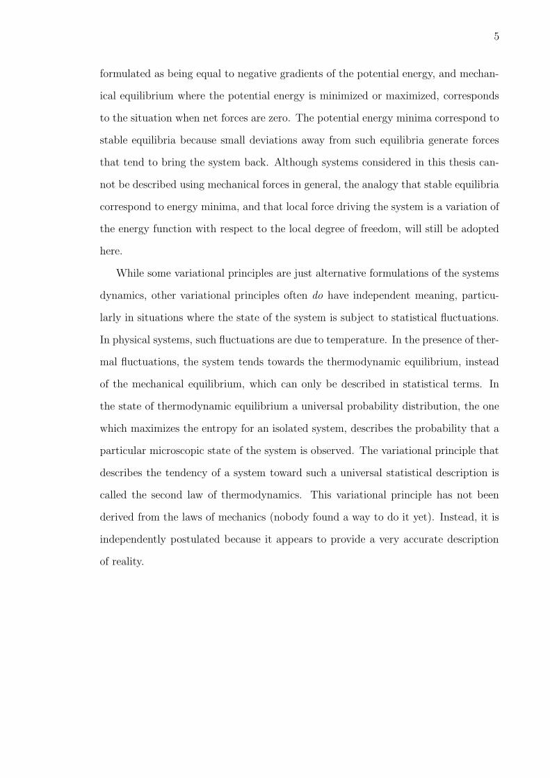
formulated as being equal to negative gradients of the potential energy, and mechan-
ical equilibrium where the potential energy is minimized or maximized, corresponds
to the situation when net forces are zero. The potential energy minima correspond to
stable equilibria because small deviations away from such equilibria generate forces
that tend to bring the system back. Although systems considered in this thesis can-
not be described using mechanical forces in general, the analogy that stable equilibria
correspond to energy minima, and that local force driving the system is a variation of
the energy function with respect to the local degree of freedom, will still be adopted
here.
While some variational principles are just alternative formulations of the systems
dynamics, other variational principles often do have independent meaning, particu-
larly in situations where the state of the system is subject to statistical fluctuations.
In physical systems, such fluctuations are due to temperature. In the presence of ther-
mal fluctuations, the system tends towards the thermodynamic equilibrium, instead
of the mechanical equilibrium, which can only be described in statistical terms. In
the state of thermodynamic equilibrium a universal probability distribution, the one
which maximizes the entropy for an isolated system, describes the probability that a
particular microscopic state of the system is observed. The variational principle that
describes the tendency of a system toward such a universal statistical description is
called the second law of thermodynamics. This variational principle has not been
derived from the laws of mechanics (nobody found a way to do it yet). Instead, it is
independently postulated because it appears to provide a very accurate description
of reality.
6
Figure 2.1: Linear RC circuit and the (non-hysteretic) dependence of the outputvoltage V0 across the capacitor on the input voltage Vi. Elliptic loop is due to thephase shift between the input and output and its size and orientation depends on thefrequency.
2.1 Hysteresis: History, rate independence and multiple time scales
What is hysteresis and what is not? Hysteresis can be defined simply as a relationship
between the state of the system and the external parameters where the state depends
on the history of the external parameters but not on their rate of variation. Depen-
dence of the state on past values of the external parameters is not all that remarkable.
Such dependences can be found even in linear systems. For example, the simple linear
circuit shown in Figure 2.1 which consists of a resistor and capacitor connected in
series would display dependence of the voltage across the capacitor V0 on the past
values of the voltage applied to the circuit Vi. In this case, however, the effect of the
past values depends on the rate at which the voltage applied to the circuit varies.
When the variation of the input voltage is sufficiently fast, a loop can be traced as
illustrated in Figure 2.1. For slow variations (variations that are small during the
time equal to the RC time constant), the voltage across the capacitor simply follows
the applied voltage Vi and no history dependence is observed. Thus, it is the lack of
dependence on the rate of the external parameter variation, as well as memory of the
past values that distinguish hysteretic systems from other much simpler systems.
7
In what types of systems can hysteresis be observed? In the above example, the
system had a single characteristic relaxation time determined by the RC constant of
the circuit. More than a single characteristic time is required for a system to display
hysteresis. Hysteresis is typically observed in those systems where, following a distur-
bance, some parts of the system re-organize well before the system as a whole reaches
thermal equilibrium with its environment. In magnets, the parts of the system that
re-organize quickly form magnetic domains. The time required for a domain to form
or re-orient is on the order of tens of nanoseconds, while relaxation to thermal equilib-
rium, when all domains are oriented randomly, can take hundreds of years. Magnetic
recording relies on the stability of such memory of the past state. In populations
of cells, individual cells can assume some state of a protein expression quickly, well
before the cellular population as a whole had a chance to randomize.
How does this separation of time scales explain emergence of hysteresis? The first
part of the explanation involves introduction of an appropriate energy functional. The
key point here is that, on a time scale longer than the fast re-organization time, one
can treat the quickly re-organizing parts of the system as single indivisible entities,
and ignore various degrees of freedom within them. This permits the redefinition
of the system’s degrees of freedom and drastically reduces their number. Such a
process is often called coarse-graining and allows the formulation of a description of
the system via an energy functional that depends only on the reduced number of the
re-defined degrees of freedom. In physics, such a reduced free energy functional is
often called Landau free energy.
Due to various constraints and the fixed disorder present (usually in the form of
inhomogeneous properties), there are hindrances to reorganization of different parts of
the system. Overcoming these hindrances requires different amounts of energy. Con-
sequently the coarse-grained Landau free energy has a complicated structure with
multiple minima separated by large barriers. When these barriers are present, the
8
Figure 2.2: Origins of hysteresis. (a) The free energy landscape as a function of statevariable M for two different values of the external parameter H. As H changes, theenergy landscape becomes distorted and transitions between different states becomepossible. (b) Due to very short time scale, the transition between different statesappears as being sharp if plotted in the state vs. external parameter plane. Whenthe external parameter returns to the original value Ha, the state variable does not,and hysteresis is displayed.
system whose state is initially arranged to be around one of the minima will tend
to linger there for a long time even in the presence of thermal fluctuations. The
lingering effect is exactly what makes the re-organization time much shorter than the
time of relaxation to thermal equilibrium. This would not have happened without
sufficiently high free energy barriers. Thus, separation of time scales inevitably leads
to the conclusion that the evolution of the system can be described by a free energy
function, which can on an intermediate time scale be treated like a potential energy
with multiple stable states. The system will rapidly re-arrange itself to minimize
this potential energy by loosing energy quickly through transfer to hidden (due to
coarse-graining) degrees of freedom.
The second part of the explanation of hysteresis involves understanding the effects
of external parameters on the free energy function. As external parameters vary, the
energy supplied to the system changes resulting in distortions of the energy landscape.
An illustration of this is shown in Figure 2.2. Let us suppose that system originally
9
occupies a state near the energy minimum at the point M1. As the external para-
meter varies and the energy landscape changes, the system remains in the original
energy minimum as long as it exists, and any change of the state variable is reversible
(Figure 2.2(a)). At some value of the external parameter (Hb), however, the original
energy minimum may disappear (at M2) and the system is forced to make a fast
transition to another energy minimum corresponding to the state M3. If after that
the external parameter returns to its original value Ha, the system will still remain
in this new energy minimum. Therefore, for any given value of external parameter
the system may be in different states corresponding to different energy minima. The
actual state assumed by the system will depend on the history of the external para-
meter variation.
The above discussion demonstrates how the separation of time scales, for fast re-
organization of system’s parts and for relaxation to thermal equilibrium, results in
dependence of the state on the history of external parameter variation. What remains
is to explain the rate independence. Rate independence is the result of adiabatic be-
havior of the system due to the separation of time scales. Adiabatic limit simply
means that external parameters do not change appreciably during the fast transition
from one stable state to another, and one can essentially ignore the details of how the
system moves between two stable states. In fact, in many experiments, transitions
between stable states can be viewed as nearly instantaneous jumps (Figure 2.2(b)).
In magnetism, such jumps are often called Barkhausen jumps. In mechanics, they
are called the Keiser effect. One can also hear such jumps when milk is poured into
a bowl of Rice Krispies cereal as it rapidly invades the pores within the cereal grains.
In summary, hysteresis owes its existence to the separation of time scales. It can
be observed only on a certain intermediate time scale, which is much longer then
the fast system dynamics but is short enough to avoid relaxation to thermal equi-
librium. Remarkably, for many systems in nature this intermediate time scale is
10
very broad. During the fast dynamics of the system energy must be dissipated into
the hidden degrees of freedom for the system to stabilize. Such energy dissipation
is called hysteresis loss. In applications outside physics, hysteresis loss may acquire
other meaning. In economic applications, for example, it will be the loss of wealth
associated with decreasing the risk or payment of commissions.
2.2 Cyclic hysteretic trajectories
The general shape of hysteresis loops depends on system constraints and symmetry
properties. Throughout most of this thesis we will consider systems with inversion
symmetries. Systems with inversion symmetry are typical in magnetism, where the
free energy is invariant with respect to changes in the sign of both the external vari-
able (magnetic field) and the state (individual spin degrees of freedom). The results
obtained for such systems can be easily extended to systems without inversion sym-
metry through the introduction of a constant bias in the external variable. However,
it is not clear to what extent are the results applicable to systems where the state
and the external variables are vector quantities.
A typical hysteresis loop for systems with inversion symmetry (magnetic systems),
is illustrated by M(H) relationship in Figure 2.3(a). H represents the external para-
meter (e.g. magnetic field), while M represents a response variable usually describing
the average state of the system (e.g. magnetization). The M(H) dependence is a
multi-valued relationship for intermediate values of the control parameter, becoming
single valued at saturation points obtained for sufficiently large magnitudes of H.
The H/M variables are often referred to also as the input/output or the field/state
variables. The loop obtained by increasing and decreasing the field H between the
saturation points is called a major hysteresis loop. The points where the field direc-
tion is reversed are called reversal points (fields). If at least one of the reversal points
11
Figure 2.3: Minor cycle types. (a) Major hysteresis loop with two minor loops inside.Minor loops 1 and 2 correspond to the same reversal fields. (b) Closed loops: C-typecycles, (c) Tilting cycles: T -type cycles, (d) Cycles with subharmonic period: S-typecycles, (e) Drifting cycles; Reptation: R-type cycles.
is smaller then the saturation, then the field cycles produce minor cycles (loops) in-
side the major hysteresis loop. Examples of minor loops obtained for different field
histories are illustrated in Figure 2.3(a). Minor loops 1 and 2 correspond to the same
reversal fields but different previous history of the field variation. Closed loops shown
in Figures 2.3(a-b) will be sometimes referred to as C-type cycles. Minor cycles,
however, do not always form loops immediately after the first external field period
and a number of periods might be necessary. Typical examples are illustrated in
Figures 2.3(c-e). The trajectory shown in Figure 2.3(c), where the reversal points
appear to move in the opposite directions will be sometimes referred to as T -cycles.
Trajectories with both reversal points moving in the same direction, illustrated in
Figure 2.3(e), will be called R-type cycles. Minor cycles with a multiple of the ex-
ternal field period are called subharmonic cycles, and will be referred to as S-type
cycles (Figure 2.3(d)). In the following section we briefly review different classes of
systems with hysteresis and classify their minor cycle behaviors whenever possible.
12
2.3 Examples of systems with hysteresis
1. Ferromagnetic materials. Ferromagnetic hysteresis has been well studied during the
past century partly due to its technological importance for the magnetic information
storage industry [1]. In most ferromagnets it is possible to freeze out thermal fluctua-
tions at sufficiently low temperatures, and within a large range of measurement time
scales the magnetization reversal processes can be viewed as independent of the mea-
surement time. Thus, ferromagnets are very convenient for studying hysteresis. Var-
ious types of hysteretic behaviors have been observed depending on the interactions
between the magnetic domains and the structural disorder present. Strict minor loop
closure (i.e. C-type behavior in Figure 2.3) has been investigated by studying the re-
peatability of Barkhausen noise patterns [2,3] and using x-ray speckle metrology [4–6].
Gradually stabilizing minor cycles have also been observed [7–11]. Clean ferromag-
nets often exhibit T -type cyclic behavior called ‘tilting’ or ‘bascule’, which has been
attributed to dipolar coupling between a few neighboring domains [12, 13]. Suffi-
ciently disordered materials exhibit R-type cycles, the effect called ‘reptation’, which
has been attributed to the interaction between a great number of domains [13–17].
2. Ordered magnetic nanostructures. In this case, the exchange interactions typ-
ical in ferromagnetic materials exist only within the nano-magnetic elements them-
selves. They are absent in the interactions between the elements of arrays, as the
only interactions existing between individual magnetic elements composing the struc-
ture are the dipolar interactions. The strength and the sign of these interactions
depends on the spacing and mutual orientations of individual elements. A review
of the main properties of magnetic nanostructures as well as various processes used
for their fabrication, such as lithography, self assembly, or growth methods, can be
found in [18]. Hysteresis studies focused mostly on relating the effects of interactions
to some features on the major loops. Relatively scarce minor loop measurements
13
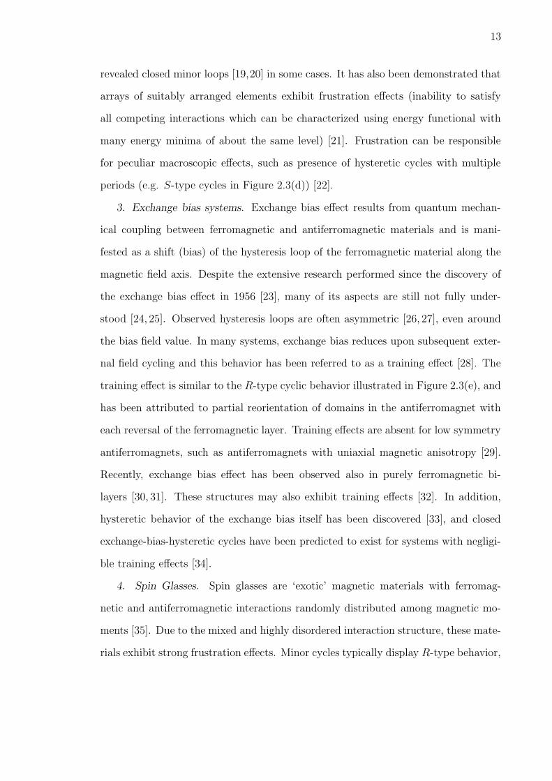
revealed closed minor loops [19,20] in some cases. It has also been demonstrated that
arrays of suitably arranged elements exhibit frustration effects (inability to satisfy
all competing interactions which can be characterized using energy functional with
many energy minima of about the same level) [21]. Frustration can be responsible
for peculiar macroscopic effects, such as presence of hysteretic cycles with multiple
periods (e.g. S-type cycles in Figure 2.3(d)) [22].
ical coupling between ferromagnetic and antiferromagnetic materials and is mani-
fested as a shift (bias) of the hysteresis loop of the ferromagnetic material along the
magnetic field axis. Despite the extensive research performed since the discovery of
the exchange bias effect in 1956 [23], many of its aspects are still not fully under-
stood [24, 25]. Observed hysteresis loops are often asymmetric [26, 27], even around
the bias field value. In many systems, exchange bias reduces upon subsequent exter-
nal field cycling and this behavior has been referred to as a training effect [28]. The
training effect is similar to the R-type cyclic behavior illustrated in Figure 2.3(e), and
has been attributed to partial reorientation of domains in the antiferromagnet with
each reversal of the ferromagnetic layer. Training effects are absent for low symmetry
antiferromagnets, such as antiferromagnets with uniaxial magnetic anisotropy [29].
Recently, exchange bias effect has been observed also in purely ferromagnetic bi-
layers [30, 31]. These structures may also exhibit training effects [32]. In addition,
hysteretic behavior of the exchange bias itself has been discovered [33], and closed
exchange-bias-hysteretic cycles have been predicted to exist for systems with negligi-
ble training effects [34].
4. Spin Glasses. Spin glasses are ‘exotic’ magnetic materials with ferromag-
netic and antiferromagnetic interactions randomly distributed among magnetic mo-
ments [35]. Due to the mixed and highly disordered interaction structure, these mate-
rials exhibit strong frustration effects. Minor cycles typically display R-type behavior,
14
which however cannot always be completely attributed to the interplay between the
interactions and disorder, and thermal effects must be included [7]. Modeling efforts
demonstrated possibility of closed minor cycles in spin-glasses with long range inter-
actions at low temperatures [36], and subharmonic S-cycles in spin glasses with short
range interactions when strong frustration effects take place [37].
5. Type-II superconductors. In type-II superconductors, hysteresis results from
the fact that as the external magnetic field changes, the flux filaments (vortices) move
and their motion is pinned by defects such as voids, normal inclusions, dislocations,
grain boundaries, compositional variations, etc. Interactions between the flux fila-
ments are of electromagnetic nature [38,39]. The resulting hysteresis behavior shows
always closed minor loops as demonstrated experimentally [40, 41].
6. Rocks. Rocks like sandstone, igneous rocks or metamorfic rocks are examples
of consolidated materials (a result of an assembly process) [42]. In these materials,
individual grains act as rigid units and the contacts between them constitute a set
of effective elastic elements (mesoscopic size cracks) that control the elastic behavior.
When external stress is applied to such a composite system, elastic elements respond
by opening or closing, depending on the magnitude of local pressure inside the rock,
and produce hysteresis effects [43]. The hysteretic length vs. pressure relationship
often displays closed minor loops [44, 45].
7. Capillary condensation. Capillary condensation of gasses adsorbed in dis-
ordered mesoporous materials refers to rapid change of a fluid inside the porous
solid from a gas-like phase to a liquid phase [46]. Hysteresis is observed in sorp-
tion isotherms that measure the amount of fluid present in the solid as the pressure
of the ambient vapor (or the chemical potential) is gradually increased and then
decreased. Capillary condensation in various porous materials reveals asymmetric
hysteretic loop shapes, where desorption (draining) occurs over a narrower range of
pressures than adsorption (filling). While smooth hysteresis loops have been observed
15
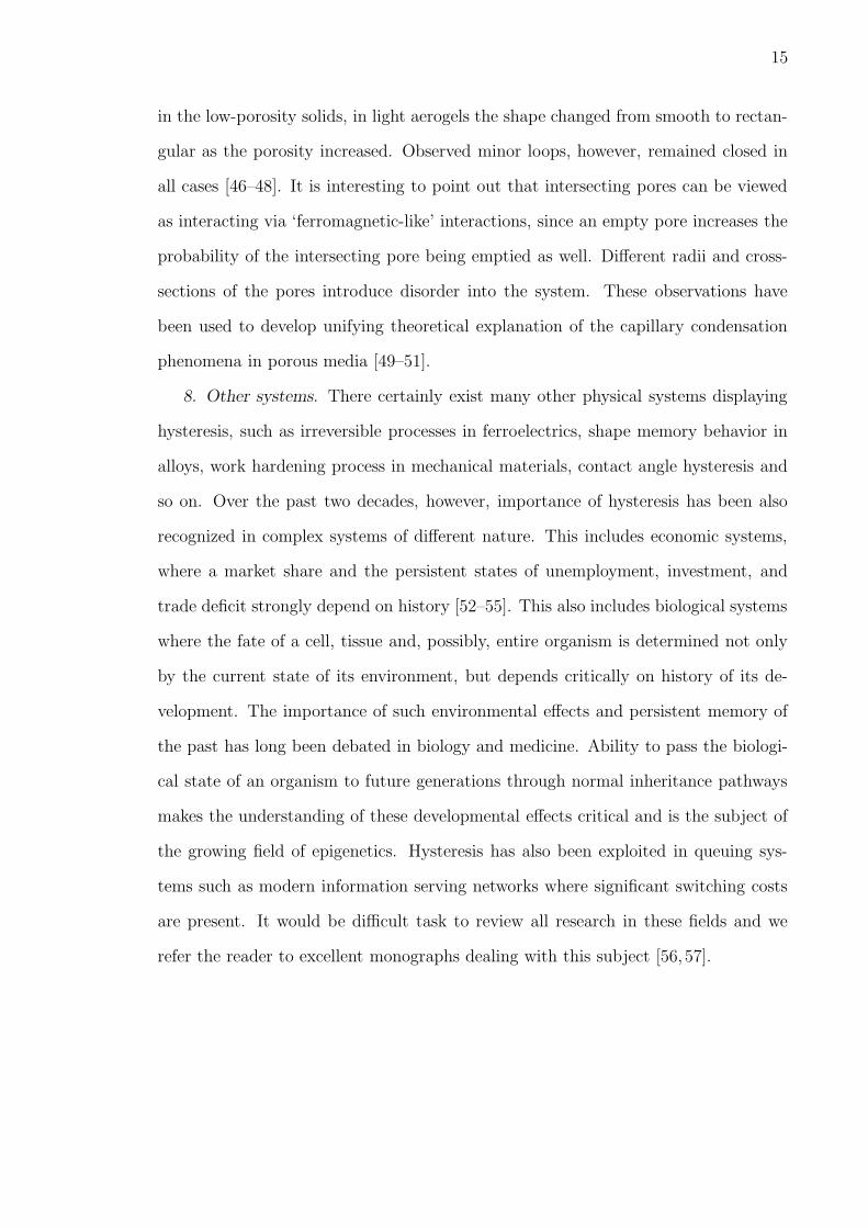
in the low-porosity solids, in light aerogels the shape changed from smooth to rectan-
gular as the porosity increased. Observed minor loops, however, remained closed in
all cases [46–48]. It is interesting to point out that intersecting pores can be viewed
as interacting via ‘ferromagnetic-like’ interactions, since an empty pore increases the
probability of the intersecting pore being emptied as well. Different radii and cross-
sections of the pores introduce disorder into the system. These observations have
been used to develop unifying theoretical explanation of the capillary condensation
phenomena in porous media [49–51].
8. Other systems. There certainly exist many other physical systems displaying
hysteresis, such as irreversible processes in ferroelectrics, shape memory behavior in
alloys, work hardening process in mechanical materials, contact angle hysteresis and
so on. Over the past two decades, however, importance of hysteresis has been also
recognized in complex systems of different nature. This includes economic systems,
where a market share and the persistent states of unemployment, investment, and
trade deficit strongly depend on history [52–55]. This also includes biological systems
where the fate of a cell, tissue and, possibly, entire organism is determined not only
by the current state of its environment, but depends critically on history of its de-
velopment. The importance of such environmental effects and persistent memory of
the past has long been debated in biology and medicine. Ability to pass the biologi-
cal state of an organism to future generations through normal inheritance pathways
makes the understanding of these developmental effects critical and is the subject of
the growing field of epigenetics. Hysteresis has also been exploited in queuing sys-
tems such as modern information serving networks where significant switching costs
are present. It would be difficult task to review all research in these fields and we
refer the reader to excellent monographs dealing with this subject [56, 57].
16
Chapter 3. Hysteresis and network models
Various models have been developed to describe magnetic hysteresis, such as the
Jiles-Atherton model, Stoner-Wolfharth model, and Globus model [1,58,59]. Models
widely used also outside the area of magnetism are the Preisach models [60] and the
Random Field Ising type models [57,61]. Since these two models are directly relevant
for the purposes of this thesis, we will review their main properties in some detail
below.
3.1 Preisach model and its properties
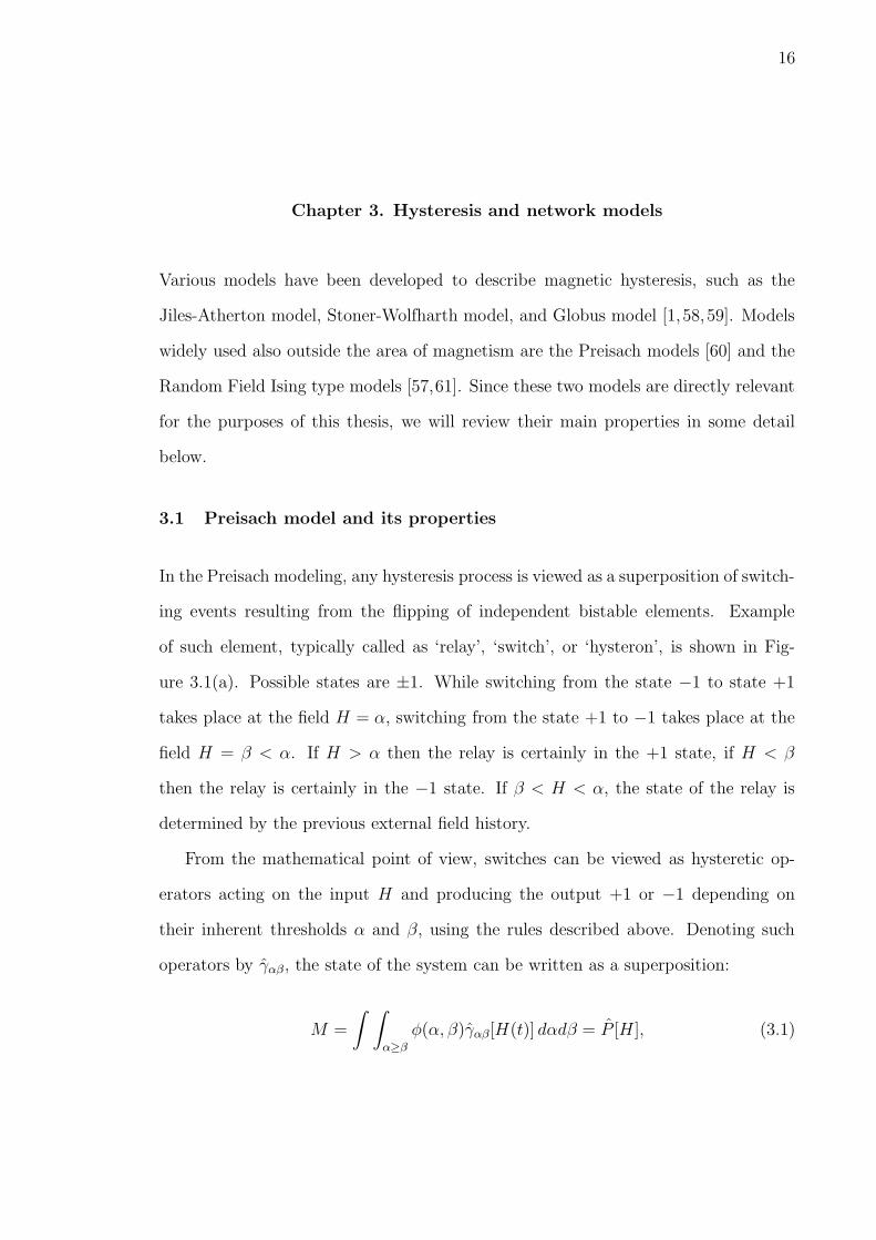
In the Preisach modeling, any hysteresis process is viewed as a superposition of switch-
ing events resulting from the flipping of independent bistable elements. Example
of such element, typically called as ‘relay’, ‘switch’, or ‘hysteron’, is shown in Fig-
ure 3.1(a). Possible states are ±1. While switching from the state −1 to state +1
takes place at the field H = α, switching from the state +1 to −1 takes place at the
field H = β < α. If H > α then the relay is certainly in the +1 state, if H < β
then the relay is certainly in the −1 state. If β < H < α, the state of the relay is
determined by the previous external field history.
From the mathematical point of view, switches can be viewed as hysteretic op-
erators acting on the input H and producing the output +1 or −1 depending on
their inherent thresholds α and β, using the rules described above. Denoting such
operators by γαβ, the state of the system can be written as a superposition:
M =
∫ ∫
α≥β
φ(α, β)γαβ[H(t)] dαdβ = P [H], (3.1)
17
Figure 3.1: Preisach model. (a) Rectangular hysteresis loop of a relay - the basicbuilding block of the Preisach model. Each relay with thresholds α and β correspondsto a point in the Preisach plane (b). The staircase interface line L separates regionswith positively and negatively flipped relays, and its shape depends on the history ofthe applied field.
where φ(α, β) is a weight function, called the Preisach distribution function, and
defines a contribution of each relay to the overall magnetization. The integral in the
Equation 3.1 is calculated over the half-plane α ≥ β. The functional relationship
between M and H given by Equation 3.1 will be referred to as a Preisach operator P .
To calculate hysteretic trajectories it is convenient to introduce a geometrical
representation of Equation 3.1. There exists a one to one correspondence between
the relays γαβ and the points (α, β) in the coordinate system defined by axes α and β.
An illustration of such a (Preisach) plane is shown in Figure 3.1(b). We will assume
that the support of the distribution φ(α, β) is finite and bounded within a triangle
defined by the line α = β and horizontal and vertical lines. The line L (discussed in
more details below) defines interface between two regions S1 and S2 with respectively
positively and negatively switched relays, for a given history of the external field H
(see below). It is easily seen that Equation 3.1 can be written as a difference between
18
the integrals over the S1 and S2 regions:
M =
∫ ∫
S1
φ(α, β) dαdβ −
∫ ∫
S2
φ(α, β) dαdβ. (3.2)
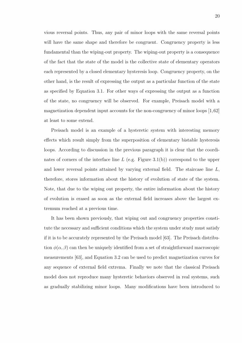
Wiping out and congruency properties. It will be discussed below that the classi-
cal Preisach model produces always closed minor loops. Consider a Preisach system
evolving under the field monotonically increasing from the negative saturation where
all relays are in the −1 state, to the point 1 on the major hysteresis loop as shown in
Figure 3.2(a). As the field H increases, relays with thresholds α < H switch to the
positive state. In the Preisach plane, the increasing field corresponds to the interface
L being a horizontal line crossing the α-axis at the value H (Figure 3.2(b)). The
areas below and above this line contain switches in the positive and negative states,
respectively. Let us suppose that at the point 1 the field is reversed and starts to
decrease. Positive switches with thresholds β < H flip to negative states. In the
Preisach plane, the decreasing field results in the addition to the interface L of the
vertical line crossing the β-axis at the value H (Figure 3.2(c)). The region to the
right contains switches which flipped back to the negative state, while the region to
the left contains switches still in the positive state. When the field is reversed again
at the point 2 and increases towards the point 1, the second horizontal part of the
interface L moves up and the relays which flipped down during the decrease from 1 to
2 are being flipped back to positive state, until the original switch-state is completely
recovered again at the point 1. This means that the minor loop generated between
the points 1 and 2 must be closed. Further field cycles between the points 1 and 2
result in flipping of the same relays (those inside the triangle in Figure 3.2(d)) back
and forth, and repeating the same loop. Similar behavior is shown in Figures 3.2(e-f)
for a minor loop obtained by different field history, after first reversing the field at
the point 3, decreasing it to the point 2, then increasing to 1 and decreasing back to
19
Figure 3.2: Wiping out and congruency properties of the Preisach model. (a) Twominor loops with the same reversal points 1 and 2 corresponding to different fieldhistories. (b-d) Evolution of state on the Preisach plane during generation of a minorloop attached to the major hysteresis. (e-f) Generation of a minor loop with the samereversal fields obtained after first reversing the field at the point 3 on the major loop.
2. The resulting Preisach diagram producing the loop closure is illustrated in Fig-
ure 3.2(f). Note, that increasing the field back to the point 3 will also generate closed
minor loop with reversal points 2 and 3. The loop closure is a general property of
a Preisach model, which has been called ‘wiping-out’ or the ‘return point memory’.
Another property of the Preisach model is the congruency property. Congruent
loops are minor loops having the same reversal fields but corresponding to different
field history, such that their geometrical shape is the same. The congruency prop-
erty is the result of the fact that the triangular areas in Figures 3.2(c) and 3.2(f)
corresponding to the same field extrema are identical. It is easily seen, by tracking
the evolution of state on the Preisach plane, that switching regions obtained for the
same reversal points will always be the same, independently of the number of pre-
20
vious reversal points. Thus, any pair of minor loops with the same reversal points
will have the same shape and therefore be congruent. Congruency property is less
fundamental than the wiping-out property. The wiping-out property is a consequence
of the fact that the state of the model is the collective state of elementary operators
each represented by a closed elementary hysteresis loop. Congruency property, on the
other hand, is the result of expressing the output as a particular function of the state
as specified by Equation 3.1. For other ways of expressing the output as a function
of the state, no congruency will be observed. For example, Preisach model with a
magnetization dependent input accounts for the non-congruency of minor loops [1,62]
at least to some extend.
Preisach model is an example of a hysteretic system with interesting memory
effects which result simply from the superposition of elementary bistable hysteresis
loops. According to discussion in the previous paragraph it is clear that the coordi-
nates of corners of the interface line L (e.g. Figure 3.1(b)) correspond to the upper
and lower reversal points attained by varying external field. The staircase line L,
therefore, stores information about the history of evolution of state of the system.
Note, that due to the wiping out property, the entire information about the history
of evolution is erased as soon as the external field increases above the largest ex-
tremum reached at a previous time.
It has been shown previously, that wiping out and congruency properties consti-
tute the necessary and sufficient conditions which the system under study must satisfy
if it is to be accurately represented by the Preisach model [63]. The Preisach distribu-
tion φ(α, β) can then be uniquely identified from a set of straightforward macroscopic
measurements [63], and Equation 3.2 can be used to predict magnetization curves for
any sequence of external field extrema. Finally we note that the classical Preisach
model does not reproduce many hysteretic behaviors observed in real systems, such
as gradually stabilizing minor loops. Many modifications have been introduced to
21
account for such effects. Preisach models with gradually stabilizing cycles have been
developed and discussed in detail in [10]. Rate dependent hysteresis effects have also
been modeled using modified classical Preisach models [64]. Another class of hys-
teresis models are the vector Preisach models where both the input and the output
variables are of a vector nature [65–68].
3.2 Random Field Ising model (RFIM)
The discussion in the previous section reveals phenomenological nature of the Preisach
model. Indeed, hysteretic relays - the basic building blocks of the Preisach model need
not to be associated with physical parts of the system and still reproduce macroscopic
hysteresis measurements. In fact, they often have to be viewed as abstract mathe-
matical objects. Different approach to hysteresis modeling is to divide the system
into basic components, such as magnetic domains or capillary pores, for example,
and explicitly specify interactions between them. Then, after defining the Landau
free energy for the system and the rules governing the evolution of state, dynamical
behavior under varying external conditions can be studied. A prototypical model for
studying hysteresis using this framework is the Random Field Ising model [57, 61].
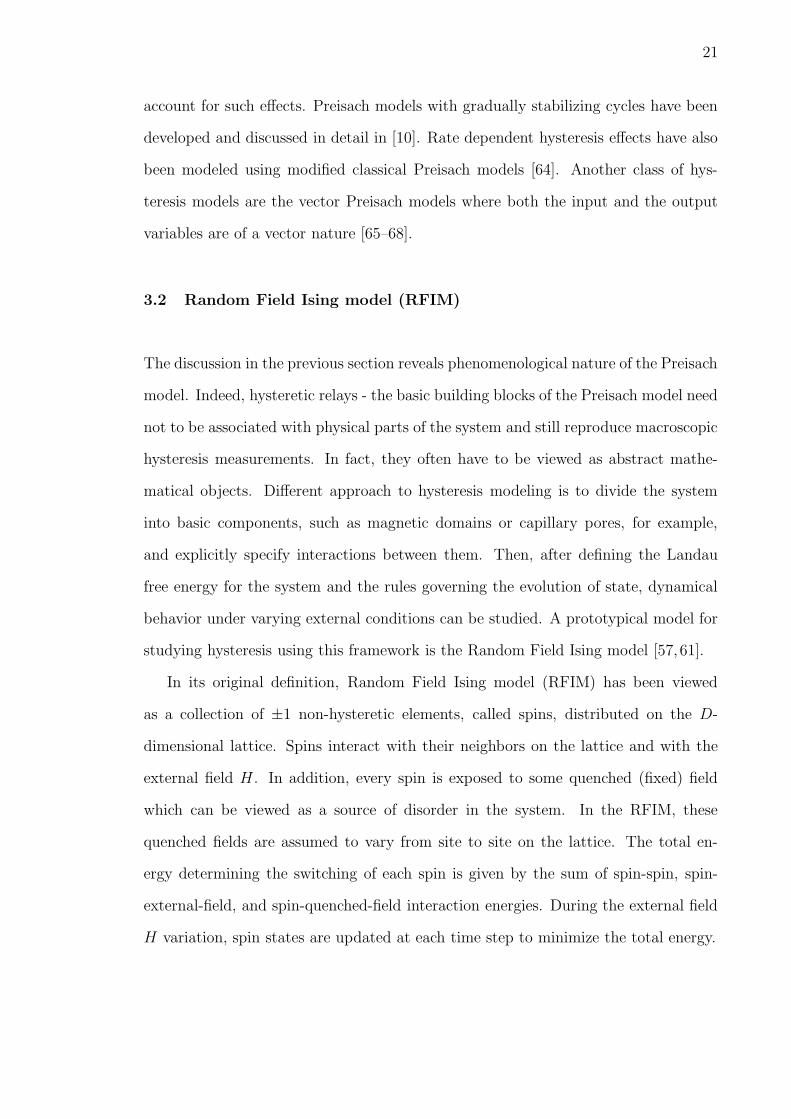
In its original definition, Random Field Ising model (RFIM) has been viewed
as a collection of ±1 non-hysteretic elements, called spins, distributed on the D-
dimensional lattice. Spins interact with their neighbors on the lattice and with the
external field H. In addition, every spin is exposed to some quenched (fixed) field
which can be viewed as a source of disorder in the system. In the RFIM, these
quenched fields are assumed to vary from site to site on the lattice. The total en-
ergy determining the switching of each spin is given by the sum of spin-spin, spin-
external-field, and spin-quenched-field interaction energies. During the external field
H variation, spin states are updated at each time step to minimize the total energy.
22
If the interactions are such that parallel alignment of spins is favored (e.g. positive
exchange interactions in ferromagnetism), then the spins flipping at a given instant of
time can trigger also neighboring spins to flip. Such events can propagate throughout
the system and result in avalanches. Due to such behavior, which is not explicitely
present1 in the Preisach model described in previous section, the RFIM has been used
as a paradigm for studying noise statistics in various out of equilibrium systems, such
as Barkhausen noise in magnets, frequency of occurrence of earthquakes, or acoustic
emission bursts generated during martensitic transformations [69]. It has been shown
that reducing the disorder relative to the spin-spin interaction strength results in the
increase of the average avalanche size. At a certain critical disorder level, infinite
avalanches spanning entire system emerge, and a steep jump appears in the originally
smooth hysteresis loop [70]. This disorder induced phase transition has been studied
in detail using the renormalization group techniques [69,71], with the main emphasis
on identifying various scaling relations, critical exponents, and determining the uni-
versality class of the RFIM. In addition, the ferromagnetic RFIM has been shown to
have a return point memory (wiping out property) and consequently produces always
closed minor cycles [70]. Unlike in the case of Preisach model, however, the congru-
ency property does not hold in general.
The RFIM model has been investigated in the contexts of many systems of dif-
fering natures, with either uniform or random interaction magnitudes between the
spins, interactions of different signs, different topological arrangements of spins, vari-
ous types of disorder, etc. This work is briefly reviewed in the following section where
we refer to this type of models jointly as ‘binary spin networks’.
1It is present implicitly through the Preisach distribution function.
23
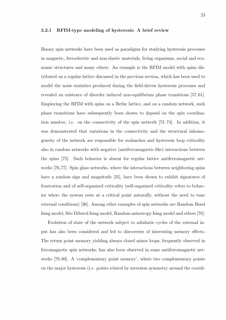
3.2.1 RFIM-type modeling of hysteresis: A brief review
Binary spin networks have been used as paradigms for studying hysteresis processes
in magnetic, ferroelectric and non-elastic materials, living organisms, social and eco-
nomic structures and many others. An example is the RFIM model with spins dis-
tributed on a regular lattice discussed in the previous section, which has been used to
model the noise statistics produced during the field-driven hysteresis processes and
revealed an existence of disorder induced non-equilibrium phase transitions [57, 61].
Employing the RFIM with spins on a Bethe lattice, and on a random network, such
phase transitions have subsequently been shown to depend on the spin coordina-
tion number, i.e. on the connectivity of the spin network [72–74]. In addition, it
was demonstrated that variations in the connectivity and the structural inhomo-
geneity of the network are responsible for avalanches and hysteresis loop criticality
also in random networks with negative (antiferromagnetic-like) interactions between
the spins [75]. Such behavior is absent for regular lattice antiferromagnetic net-
works [76,77]. Spin glass networks, where the interactions between neighboring spins
have a random sign and magnitude [35], have been shown to exhibit signatures of
frustration and of self-organized criticality (self-organized criticality refers to behav-
ior where the system rests at a critical point naturally, without the need to tune
external conditions) [36]. Among other examples of spin networks are Random Bond
Ising model, Site Diluted Ising model, Random anisotropy Ising model and others [78].
Evolution of state of the network subject to adiabatic cycles of the external in-
put has also been considered and led to discoveries of interesting memory effects.
The return point memory yielding always closed minor loops, frequently observed in
ferromagnetic spin networks, has also been observed in some antiferromagnetic net-
works [79, 80]. A ‘complementary point memory’, where two complementary points
on the major hysteresis (i.e. points related by inversion symmetry around the coordi-
24
nate origin) have identical microstates, has been observed in spin glass networks with
short range interactions at non-zero temperature [81]. Studies of spin-glass networks
also led to discovery of the ‘reversal field memory’ where a certain reversal curve
inside the major hysteresis loop appears to remember the negative of its reversal
field. This memory effect has been shown to be due to the local spin-reversal sym-
metry of the associated Hamiltonian [82]. Only a few works dealing with analysis of
systems displaying a gradual convergence to minor loops and multi-cycling behavior
seem to be available [22,37,80,83,84]. Such studies typically employed regular-lattice
spin networks with antiferromagnetic and magneto-static interactions. Among many
questions remaining to be answered are: What is the effect of interactions versus the
disorder on the hysteresis cycles? How does the connectivity of the network influ-
ence the rate of a minor loop formation? Are topological features of the network
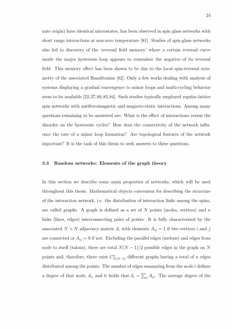
important? It is the task of this thesis to seek answers to these questions.
3.3 Random networks: Elements of the graph theory
In this section we describe some main properties of networks, which will be used
throughout this thesis. Mathematical objects convenient for describing the structure
of the interaction network, i.e. the distribution of interaction links among the spins,
are called graphs. A graph is defined as a set of N points (nodes, vertices) and n
links (lines, edges) interconnecting pairs of points. It is fully characterized by the
associated N ×N adjacency matrix A, with elements Aij = 1 if two vertices i and j
are connected or Aij = 0 if not. Excluding the parallel edges (melons) and edges from
node to itself (talons), there are total N(N − 1)/2 possible edges in the graph on N
points and, therefore, there exist CnN(N−1) different graphs having a total of n edges
distributed among the points. The number of edges emanating from the node i defines
a degree of that node, di, and it holds that di =∑
j Aij. The average degree of the
25
Figure 3.3: Examples of various graph structures: (a) Trees of the order k = 6. Alinear chain of spins can be represented by a tree like graphs. (b) Cycle of orderk = 6. The square lattice contains cycles of different orders starting from k = 4. (c)Complete subgraphs of order k = 3, 4, 5.
network is d = 〈di〉 = N−1∑
ij Aij. Any set of nodes and edges chosen from the graph
defines its subgraph. Graphs (subgraphs) can assume various topological structures.
Examples are cycles, trees or complete subgraphs. A cycle of order k is defined as a
closed loop of k edges such that every two consecutive edges, and only those two, have
a common node (Figure 3.3(b)). A tree of order k is a connected graph with k points
and k − 1 edges such that none of its subgraphs is a cycle. Examples are shown in
Figure 3.3(a). Note that a linear chain of spins can be viewed as network with a tree
like structure having d = 2, and that a two-dimensional lattice of spins with d = 4
contains also cycles (Figure 3.3(b)). A complete subgraph of order k (often referred
to as clique of size k) is a set of k points where each point is interconnected with
every other point. Example in Figure 3.3(c) contains total 15 complete subgraphs of
order three, 5 subgraphs of order four and 1 subgraph of order five.
3.3.1 Classical random graphs (Erdos-Renyi)
Complex networks with often unknown organizing principles and complex topology
frequently appear random [85]. A convenient mathematical framework for studying
such objects is the random graph theory, which deals with graphs with a randomly
26
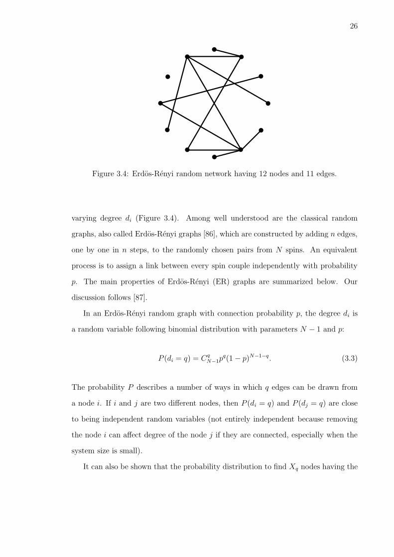
Figure 3.4: Erdos-Renyi random network having 12 nodes and 11 edges.
varying degree di (Figure 3.4). Among well understood are the classical random
graphs, also called Erdos-Renyi graphs [86], which are constructed by adding n edges,
one by one in n steps, to the randomly chosen pairs from N spins. An equivalent
process is to assign a link between every spin couple independently with probability
p. The main properties of Erdos-Renyi (ER) graphs are summarized below. Our
discussion follows [87].
In an Erdos-Renyi random graph with connection probability p, the degree di is
a random variable following binomial distribution with parameters N − 1 and p:
P (di = q) = CqN−1p
q(1 − p)N−1−q. (3.3)
The probability P describes a number of ways in which q edges can be drawn from
a node i. If i and j are two different nodes, then P (di = q) and P (dj = q) are close
to being independent random variables (not entirely independent because removing
the node i can affect degree of the node j if they are connected, especially when the
system size is small).
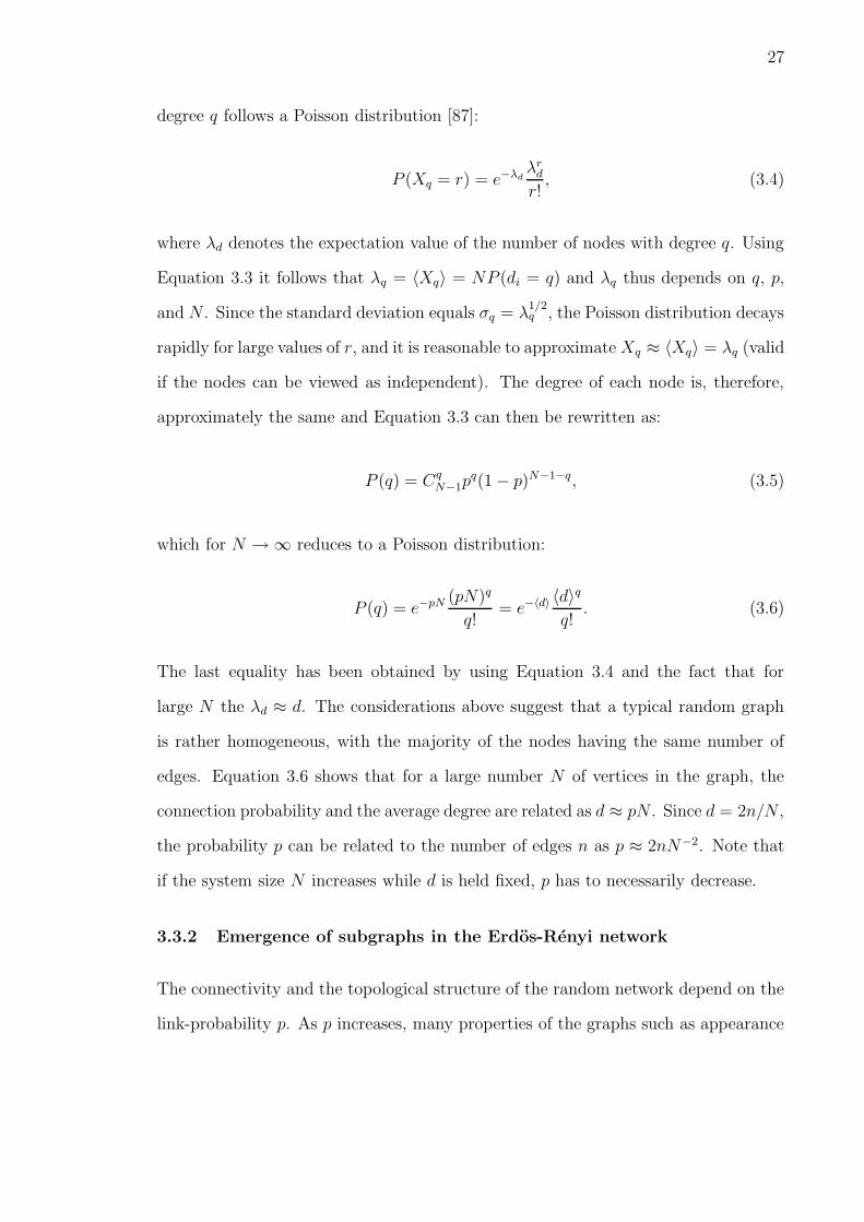
It can also be shown that the probability distribution to find Xq nodes having the
27
degree q follows a Poisson distribution [87]:
P (Xq = r) = e−λdλrdr!, (3.4)
where λd denotes the expectation value of the number of nodes with degree q. Using
Equation 3.3 it follows that λq = 〈Xq〉 = NP (di = q) and λq thus depends on q, p,
and N . Since the standard deviation equals σq = λ1/2q , the Poisson distribution decays
rapidly for large values of r, and it is reasonable to approximate Xq ≈ 〈Xq〉 = λq (valid
if the nodes can be viewed as independent). The degree of each node is, therefore,
approximately the same and Equation 3.3 can then be rewritten as:
P (q) = CqN−1p
q(1 − p)N−1−q, (3.5)
which for N → ∞ reduces to a Poisson distribution:
P (q) = e−pN(pN)q
q!= e−〈d〉 〈d〉
q
q!. (3.6)
The last equality has been obtained by using Equation 3.4 and the fact that for
large N the λd ≈ d. The considerations above suggest that a typical random graph
is rather homogeneous, with the majority of the nodes having the same number of
edges. Equation 3.6 shows that for a large number N of vertices in the graph, the
connection probability and the average degree are related as d ≈ pN . Since d = 2n/N ,
the probability p can be related to the number of edges n as p ≈ 2nN−2. Note that
if the system size N increases while d is held fixed, p has to necessarily decrease.
3.3.2 Emergence of subgraphs in the Erdos-Renyi network
The connectivity and the topological structure of the random network depend on the
link-probability p. As p increases, many properties of the graphs such as appearance
28
Figure 3.5: Evolution of a graph structure. Different topological elements appearsuddenly at specific probabilities p.
of trees, cycles, or cliques emerge suddenly at some critical probability Pc, similarly to
phase transition behavior occurring in physical systems [88]. The values of Pc depend
on the network size N . It is convenient to express the dependence of probabilities
on the network size as a power law p ≈ N z, where z is a tunable parameter varying
between −∞ and 0, and then follow the evolution of a graph structure as z increases
(Figure 3.5). For z < −3/2 almost all graphs contain only isolated nodes and edges.
When z passes through −3/2, trees of order 3 suddenly appear. Trees of order 4
appear as soon as z exceeds −4/3. As z approaches −1, graph contains trees of larger
and larger order. However, as long as z < −1 which means that average degree of
the graph d = pN → 0 as N → ∞, the graph is composed only of disconnected trees.
When z passes through −1, the asymptotic probability of cycles of all orders jumps
from 0 to 1, even though z is changing smoothly. Note that cycles of order 3 can also
be viewed as complete subgraphs of order 3. Complete subgraphs of order 4 appear
at z = −2/3, and as z continues to increase, complete subgraphs of larger and larger
order emerge. As z → 0 almost every random graph approaches a complete graph of
size N .
29
It has also been shown that there exists an abrupt change in the cluster structure of a
random graph as d→ 1. For d < 1 there are relatively few edges and all components
(subgraphs) are small, having an exponential size distribution and a finite mean size.
However, when d ≥ 1, an extensive fraction of all vertices are joined together in a
single giant component and graph becomes well connected.
30
Chapter 4. Random Coercivity Interacting Switch model (RCIS)
The Preisach and the RFIM models do not reproduce certain experimental obser-
vations, such as the T and R cycles illustrated in Figure 2.3. Although there exist
modifications of the Preisach model which account for the R-type cycles [10], they
are purely phenomenological and do not yield information about the nature of the
cycle opening and its relation to the structure and the disorder in the system. On
the other hand, while the RFIM with positive interactions (ferromagnetic) has strict
return point memory property [70], and thus always closed minor loops, the RFIM
model with negative interactions displays only almost negligible hysteretic effects [76].
For these reasons we developed different physically motivated model, called Ran-
dom Interacting Switch model (RCIS), which reproduces these aspects of hysteresis
not seen in the Preisach or RFIM models, and allows studying the relationship be-
tween the types of minor cycles and the structure of interactions and disorder.
4.1 Definition
The Random Coercivity Interacting Switch model (RCIS) combines the Preisach
model and RFIM discussed in Sections 3.1 and 3.2. It is a collection of N inter-
acting spins si, with +1 or −1 being the only allowed states. Switching of each spin
is described by a rectangular hysteresis loop with symmetric thresholds ±αi, αi > 0.
The thresholds αi are viewed as random variables with probability distribution ρ(α),
and mimic structural disorder in the system. Such classical hysteretic spins are fre-
quently used as representations of single domain magnetic grains, tiny capillary pores
in absorbing materials, vortex pinning imperfections in superconductors, individual
decision making agents in socio-economic systems, etc. [57].
31
Figure 4.1: (a) Rectangular hysteresis loop corresponding to the switch si with sym-metric thresholds αi and βi = −αi, shifted from the coordinate origin due to theinteraction with the neighboring spins. (b) When the interaction is equal to zero, allspins with symmetric thresholds lie in the Preisach plane on the line perpendicularto β = α line. For nonzero interactions, both thresholds are shifted by an amount∆i, which depends on the interaction strength and on the state of the neighbors ofthe spin si.
The spins si and sj will be assumed to interact via pair-wise interactions described
by a matrix Jij = δJAij, where J is a positive constant representing the interaction
strength, δ equals either +1 or −1 depending on whether the system is of ferro-
magnetic or antiferromagnetic nature (i.e. if parallel or anti-parallel alignment of
neighboring spins is preferred). The matrix Aij is N × N adjacency matrix of the
associated graph, with elements Aij = 1 if the spins si and sj interact and Aij = 0 if
they do not interact, and describes topological structure of interactions.
In the absence of interactions, spins flip whenever the external field H matches
their switching thresholds. Generally, however, the flipping of any spin si will be
determined by a local field hi, dependent on the external field and also on the con-
tribution from interactions of si with other spins. We assume that hi can be written
32
as a sum:
hi = H +N
∑
j=1
Jijsj = H + ∆i (4.1)
where the symbol ∆i denotes an interaction field due to the neighbors of si. ∆i deter-
mines a shift of the originally symmetric rectangular loop with thresholds ±αi from
the coordinate origin (Figure 4.1(a)). This shift can also be depicted in the Preisach
α-β plane, as shown in Figure 4.1(b). To any spin si with symmetric thresholds, there
corresponds a point (−αi, αi) on the line α = −β in the α-β plane. When the inter-
action field ∆i is nonzero, this point is shifted to (−αi + ∆i, αi + ∆i). As the system
evolves and neighboring spins flip back and forth, the ∆i changes and the points in
the plane change their position accordingly. It is easy to see, following the rules in-
troduced in Section 3.1 and Equation 4.1, that the points in the Preisach plane move
along with the external fieldH line if the interactions are negative (antiferromagnetic),
and they move against the field if the interactions are positive (ferromagnetic). Due
to the presence of disorder and nontrivial interaction topologies, details of this mo-
tion are complicated, often resulting in a breaking of the return point memory and
the congruency properties. This demonstrates the difference between the RCIS and
Preisach models.
4.2 Adiabatic dynamics
The spin state of the system remains stable as long as the local fields of all spins
remain greater or smaller then their upper and lower thresholds, i.e. as long as
hisi > −αi holds for any spin si. As the external field H evolves, hi changes according
to Equation 4.1. Flipping occurs as soon as hisi < −αi, and the evolution of the
system towards the next stable state proceeds according to the following rules:
R1. In a pre-defined order, update the state of every relay one at a time according
33
to:
sk(n + 1) =
+1 if hk(n) ≥ +αk
−1 if hk(n) ≤ −αk.
sk(n) otherwise
(4.2)
R2. If all relays end up in the stable state go to R3, otherwise repeat R1.
R3. Increment the input H by the smallest possible amount ∆H required to induce
switching of at least one relay si in the RCIS network.
In general, the steps R1 and R2 need to be repeated a number of times until the
stable state of the RCIS is reached. While the state of the RCIS varies during this
stabilization, the external field H remains fixed. Such relaxation process mimics many
behaviors known in the physical sciences, such as a Barkhausen jump (magnetism)
or an avalanche (earthquake), for example. Moreover, the relationship between the
input and the stable state of an RCIS network (or any function of it) is the same
regardless of the rate of input variation and therefore the dynamics R1−R3 produces
rate-independent hysteresis behavior. The dynamics R1 −R3 is often used to model
processes when thermal fluctuations are absent, and is often referred to as a field
To prove that repeated iterations of steps R1 − R2 converge to a stable state, it is
convenient to define the state function based on the analogy with the RFIM:
G = −1
2
∑
ij
Jijsisj −H∑
i
si. (4.3)
The first term in the Equation 4.3 is the spin-spin interaction energy, while the
second term describes the interaction of individual spins with the external field. We
34
now observe that:
−∆G
∆si= H +
N∑
j=1
Jijsj = hi, (4.4)
where hi is the local field defined by Equation 4.1. The switching rule R1 implies:
0 < hi∆si = −∆G
∆si∆si = −∆G. (4.5)
Since only one relay can be switched at a time n, the state function G necessarily
decreases during any switching event. Moreover, G is always bounded from below, and
thus the switching process R1 − R2 must terminate after reaching a local minimum
of G.
The function G can be viewed as a free energy function of the RCIS network.
It is important to note, that there is also a double well free energy associated with
individual hysteretic spins. Due to the symmetry of thresholds of spins, however,
this free energy is the same in their negative and positive states, and its addition in
Equation 4.3 would only add a constant that would not affect any further results.
This argument does not hold for non-symmetric relays, which will not be considered
in this work.
4.4 Single spin flip dynamics limit
According to Section 4.2, avalanches are multiple switching events consisting of many
spins flipping at a given field. If during the step R1 more then one spin becomes
unstable, then we flip all unstable spins in a predefined sequence starting from the
spin with the largest sum hisi + αi (force). However, are the resulting stables states
independent of the actual order in which the unstable spins are updates? Or in other
words: Do different updating sequences produce the same state of the system? As it
turns out, the same final state is obtained independently of the order of updating only
35
if the interactions are positive Jij > 0 [74]. If the interactions are negative Jij < 0,
different final states are obtained depending on the order of the flipping the spins [77].
The procedure for choosing the correct order of updating in this case remains unclear.
This issue can be partially resolved in the present RCIS model. In the low inter-
action limit, the dynamics R1−R3 introduced in Section 4.2 reduces to a very simple
regime with trivial avalanches consisting of single spin flips only. The argument is as
follows. While avalanches in the ferromagnetic RCIS consist of spins always flipping
along the external field direction (i.e. ∆H∆si > 0), in the antiferromagnetic case
avalanches are nontrivial and can contain spin flipping both ways, along and against
the external field direction. Due to the antiferromagnetic interactions, the local fields
on the neighbors of some spin si flipping along the field H become reduced. If the
interaction magnitude J is sufficiently large, then such a decrease of local fields may
trigger some of these neighbors to flip against the field H. As it turns out, how-
ever, there exists an interaction limit, Jt, such that back-flips must be absent as long
as J < Jt. Denoting the minimum threshold magnitude from among all spins in
the system by αmin = min(αi), the maximum degree (the degree of a node equals
to the number of links emanating from it; Section 3.3) present in the network by
dmax = max(di), and given the Equation 4.1, the backward transitions will clearly be
impossible in the RCIS if max(∆i) = max(di)J |si| < αmin. This relation defines the
limiting interaction magnitude:
Jt = αmin/dmax. (4.6)
For J < Jt the back-flips will be absent, the avalanches trivial, consisting of single
spin transitions when ∆H∆si > 0, and the state dependence will be a monotonic
function of external field H. In fact, this behavior is realistic for magnetic films with
very strong perpendicular anisotropy for example [18, 89].
36
In this thesis we will often employ a Gaussian distribution of thresholds. The mean
and the variance of the distribution will be denoted respectively by µ and σ, and we
will always assume that µ >> σ. Truncating the thresholds αi below αmin = µ− 3σ,
when the probability for observing αi < αmin becomes negligible, allows specifying
the weak interaction limit using Equation 4.6 as:
Jt = (µ− 3σ)/dmin. (4.7)
Note that due to the truncation of the random thresholds below αmin, the threshold
distribution slightly differs from the Gaussian. We also considered other distributions,
including log-normal and uniform, which all yielded results qualitatively similar to
those presented in this thesis.
4.5 Summary
In this chapter we defined the RCIS model which will be used next to investigate
behavior of cyclic trajectories and their relation to the structure of interactions and
disorder. The RCIS model can be viewed as a combination of the Preisach and RFIM
models. Its main new property, when compared to previous models, is the single spin
flip dynamical limit which allows thermodynamically consistent analysis even in the
case of negative interaction networks. As will be shown in this thesis, RCIS model
reproduces many qualitative features of hysteresis observed in nature.
37
Chapter 5. Mean field models: From closed to open cycles
In this chapter we use the RCIS model to investigate origins of the cycle opening.
We show that networks with positive (ferromagnetic) interactions produce always
closed minor loops. This is due to the return point memory property (RPM), which
will be shown to hold for ferromagnetic networks of an arbitrary adjacency matrix.
No such general statements can be made about networks with negative interactions
(antiferromagnetic), and in fact antiferromagnetic networks generally do not produce
closed cycles. However, there are some cases where the RPM still holds. As an
example we discuss mean field RCIS model with spins on a fully connected network.
We then show that a modification of such system obtained by dividing the interaction
network to form two interacting mean field RCIS models produces new behavior,
where open cycles emerge suddenly at some critical interaction. This result suggests
that both the RPM (Figure 5.1A(a-b)) and the cycle opening (Figure 5.1B(a-b))
could be observed in some antiferromagnetic networks, depending on their structural
parameters.
5.1 Cycle closure in the positive interaction networks: Return PointMemory (RPM)
The fact that the RPM property holds for RCIS model with positive interactions
can be shown similarly as demonstrated previously for the ferromagnetic RFIM
model [70]. Only a few straightforward modifications need to be introduced, which
account for the hysteretic nature of spins and the fact that we consider networks with
an arbitrary adjacency matrix.
Assume a spin network with adjacency matrix Aij and the spin-spin interaction
strength J > 0. Let any two spin states of the system be denoted by the vectors
38
−10 −5 0 5 10−1
−0.5
0
0.5
1
M
H4.4 4.6 4.8 5
0.52
0.54
0.56
0.58
H
−10 −5 0 5 10−1
−0.5
0
0.5
1
M
H4.8 4.9 5 5.1
0.12
0.14
0.16
0.18
0.2
0.22
H
(A−a) (A−b)
(B−a) (B−b) 1.cycle 2.cycle
3.cycle
3 cycles
Figure 5.1: A(a-b) Minor loop cycled 3 times showing complete closure at the end ofthe first cycle for interaction weaker than the critical point. B(a-b) 3 minor cyclesshowing opening for interaction stronger than the critical point.
s = s1, s2, . . . , sN and z = z1, z2, . . . , zN. The states s and z will be called par-
tially ordered if si ≥ zi for every i (or if si ≤ zi for every i). One very important
property of ferromagnetic networks is that the partial ordering of states remains pre-
served under the field driven adiabatic dynamics defined in Section 4.2. If the spin
states s and z attained respectively at fields Hs and Hz ≤ Hs are ordered at some
initial time, then their ordering will remain preserved under the field variation as long
as the condition Hz ≤ Hs holds.
The proof of this property follows by reaching the contradiction. Assume the or-
dering s ≥ z, which holds at some initial time for Hs ≥ Hz. This partial order would
39
be violated as soon as some spin zi flips before si anytime during the evolution under
Hs ≥ Hz. Observe, that if the spin zi is to flip before si (i.e. if si ≤ zi is to happen) at
some instant of time, the corresponding local fields given by Equations 4.1-4.2 must
at that time satisfy the inequality:
hsi = J∑
j
Aijsj +Hs ≤ hzi = J∑
j
Aijzj +Hz. (5.1)
However, since 1) Hs ≥ Hz holds by requirement, 2) J∑
j Aijsj ≥ J∑
j Aijzj be-
cause all neighbors around the node i still remain ordered at that time instant, and
3) noting that both zi and si are at the node i and therefore have the same threshold
αi, then any event yielding si ≤ zi is impossible. Thus the partial order remains pre-
served under the dynamics at all times. The above argument holds for any adjacency
matrix Aij of the network as long as J remains positive.
The preservation of partial ordering and the adiabatic dynamics condition (Sec-
tion 4.2) guarantee that the final state of the system, which evolves under an external
field arbitrarily changing between two limits (bounds), depends only on the final
value of the external field. The final state does not dependent on the duration of
the field variation or on the history, as long as the field remains within the bounds.
As a consequence, minor cycles obtained by cycling the field between two reversal
points must recover the same spin state after each cycle, demonstrating the RPM.
The proof of this property is identical as for the RFIM and details can be found
in [70]. The RPM is a remarkable property that seems to hold in many systems in
nature. Several examples, such as e.g. ferromagnets, type-II superconductors, and
capillary condensation in porous media can be found in Section 2.3.
40
5.2 Cycle closure in the negative interaction networks
The proof of the RPM for the RCIS given in the previous section applies only to
the positive interaction case. However, RPM holds also for some specific networks
with negative interactions. As an example of such an antiferromagnetic system, we
consider an RCIS model with spins on a fully connected network. Since systems with
fully connected interaction networks are typically called mean field models, we adopt
the same terminology. Minor loop behavior in the mean field RCIS model has been
studied previously in the context of the moving Preisach model [90], and the RPM
property has been shown to hold for both positive and negative interactions [62]. Here
we present alternative (informal) argument demonstrating the RPM property in the
mean field RCIS model.
For a fully connected interaction network, all off-diagonal elements of the N ×N
adjacency matrix are equal to 1, and according to Equation 4.1, the local fields hi
can be expressed as
hi = H − J ′M, (5.2)
where J ′ = NJ , M = N−1∑
j sj is the average state of the system (magnetization)
and the ‘−’ sign is due to the antiferromagnetic nature of interactions. Note that
since hi is the same for every spin, the state of spins depends only on the variables
H and M , or more precisely, on the difference H − J ′M . The functional dependence
of the spin’s state can be expressed as si = si(H − J ′M) and the magnetization as:
M =1
N
∑
i
si(H − J ′M) = P [H − J ′M ], (5.3)
where P is a Preisach operator introduced in Section 3.1. Note that the Preisach
operator in Equation 5.3 depends also on the output variable M . For this reason the
model defined by Equation 5.3 has been called moving Preisach model [90].
41
The RPM can be demonstrated as follows. Consider the single spin flip dynamics
limit defined in Section 4.4. The back-flipping spins do not exist then, the difference
H−J ′M increases (decreases) whenever the external fieldH increases (decreases), and
the dependence of M on H given by Equation 5.3 must be monotonic (i.e. ∆M∆H ≥
0). Consequently, the operator relationship:
H = P−1[M ] + JM = Γ[M ] (5.4)
obtained by inverting the Equation 5.3 must also be monotonic. Since the closed
loops generated by a monotonic hysteresis relationship map into closed loops of its
inverse, the Preisach model P−1 also exhibits the RPM. The addition of the linear
term J ′M in Equation 5.4 does not change this fact since it only tilts the hysteresis
loops. Thus, the operator Γ has the RPM and monotonicity properties, implying the
same for its inverse M = Γ−1(H).
Note, that if the above argument holds for any network size N , then also the
ensembles of spins forming couples, cycles of size 3, and cliques of any size will have
the RPM property, and therefore display closed cycles.
5.3 Neel’s mean field model: Transition between RPM and open cycles
Consider two groups of spins, such that the spins within each group do not interact
with each other. This situation is illustrated in Figure 5.2, where the spins on the
lattice are divided into two interpenetrating sub-lattices A and B. Magnetizations
(average states) of each sub-lattice are Ma and Mb and the total magnetization in
the system is an average M = (Ma +Mb)/2. While the spins within the sub-lattice
do not interact with each other, every spin sAi from sub-lattice A interacts with all
spins sBi from the sub-lattice B via the same mean field −J ′Mb, and every spin
sBi from sub-lattice B interacts with all spins from sub-lattice A via the mean field
42
Figure 5.2: Neel’s lattice. Shown are two interpenetrating lattices A and B (whiteand black dots) of spins. Magnetizations of each sub-lattice are Ma and Mb. Spinsdo not interact within the sub-lattice. Interaction is only between the spins fromdifferent lattices via the mean fields −J ′Ma and −J ′Mb, where J ′ is the interactionmagnitude. Magnetization of the entire system is an average M = (Ma +Mb)/2.
interaction −J ′Ma (J ′ > 0). This structure of interactions is analogous to the Neel’s
approximation used to describe magnetism of antiferromagnetic materials [91].
Following Equations 5.2-5.3, the effective fields ha and hb responsible for switching
within sub-lattices A and B respectively, can be defined as
ha = H − J ′Mb and hb = H − J ′Ma, (5.5)
where J ′ = JN/2. In the following we drop the prime and denote the interaction
strength simply by J . The average states Ma and Mb in Equation 5.5 can then be
expressed as:
Ma =2
N
∑
i∈A
sAi (H − JMb) = P [H − JMb] = P [ha], (5.6)
Mb =2
N
∑
i∈B
sBi (H − JMa) = P [H − JMa] = P [hb], (5.7)
with N/2 being the number of spins within a sub-lattice, and P the Preisach hys-
teresis operator. Thus, the Neel’s type mean-field RCIS model (NMF) is one where
43
two identical Preisach hysteresis operators are coupled to each other. The coupling
constant J > 0 corresponds to the strength of the antiferromagnetic interaction.
5.3.1 RPM in the Neel’s mean field model (NMF)
Consider the single spin flip dynamics limit defined in Section 4.4. Assuming that the
external field H increases starting from the negative saturation, the dependences of
the sub-lattice magnetizations Ma and Mb on H can be expressed via the following
coupled integral equations:
Ma = −1 + 2
∫ −JMb+H
−∞
ρ(α) dα, (5.8)
Mb = −1 + 2
∫ −JMa+H
−∞
ρ(α) dα, (5.9)
where ρ(α) is a spin threshold probability distribution. We assumed that the number
of spins in each sub-lattice is sufficiently large, such that ρ(α) can be viewed as a
smooth function, and hence we can replace the summations in Equations 5.6-5.7 by
an integration. Subtracting the second equation from the first and changing the
variables to M = (Ma + Mb)/2 and ψ = (Ma −Mb)/2, gives after arrangement the
relation:
ψ =
∫ +Jψ
−Jψ
ρ(α− JM +H) dα. (5.10)
After substituting α→ Jψα, the above expression reduces to:
ψ = Jψ
∫ +1
−1
ρ(Jψα− JM +H) dα, (5.11)
or equivalently:
ψ
(
1 − J
∫ +1
−1
ρ(Jψα− JM +H) dα
)
= 0. (5.12)
44
Since ρ(x) is the probability distribution, and thus ρ ≥ 0 for every x, the following
inequality certainly holds:
0 ≤
∫ +1
−1
ρ(x) dx ≤
∫ +1
−1
ρmax dx = 2ρmax, (5.13)
where ρmax is the maximum of the probability distribution ρ. Therefore, if 2Jρmax ≤ 1,
Equation 5.12 will have only a trivial solution ψ = 0 (which implies Ma = Mb).
Nontrivial solutions ψ 6= 0 (Ma 6= Mb) are technically possible if 2Jρmax ≥ 1. Hence,
the critical interaction at which qualitatively new solutions appear equals to:
Jc =1
ρmax. (5.14)
We now show that RPM holds for J < Jc. The argument can be divided into three
steps: 1) If ψ = Ma−Mb = 0, then the local fields ha = hb = h and Equations 5.6-5.7
can be rewritten as:
Ma = Mb = P [h]. (5.15)
Since the Preisach operator P has the RPM property, closed cycles of h must re-
sult in closed cycles of both Ma and Mb. Moreover, the operator relation given by
Equation 5.15 is invertible because the threshold distribution ρ is smooth and non-
negative and the inverse P−1 is also a Preisach operator [57, 92]. As a result, the
relations h = P−1[Ma] and h = P−1[Mb] also have RPM property, i.e. closed magne-
tization cycles must produce closed h-cycles. 2) Using Equation 5.5, the relationship
between H and h can be written as
H = JP [h] + h = N [h], (5.16)
45
where N [h] is again a Preisach operator, since the first term in Equation 5.16 is a
Preisach operator and the addition of a linear term h just tilts the hysteresis loops.
Hence, the relationship given by Equation 5.16 has to have the RPM, as well as the
inverse. 3) Using the fact that relations defined by Equations 5.15-5.16 and their
inverses have the RPM, the relations Ma(H) = Mb(H) must also have RPM. This
proves the existence of closed cycles for interactions J below the critical strength Jc.
5.3.2 Cycle opening in the NMF
As shown in the previous section, nontrivial solutions of Equation 5.12 are possible if
J > Jc. To see that such solutions exist, we solve Equation 5.12 numerically assum-
ing a Gaussian distribution of thresholds ρ(α). Note that given the relation defined
by Equation 5.14, the critical interaction Jc can be related to the variance σ of the
Gaussian distribution simply as Jc = σ√
π/2. The critical interaction is therefore
directly determined by the disorder level present in the system.
Dependence of ψ = Ma−Mb on the field point H along the increasing branch of
the hysteresis loop M(H) is plotted in Figure 5.3. Different interaction magnitudes
below and above the Jc are considered. Figure shows that the difference ψ is zero
for J < Jc, becoming nonzero for J > Jc and growing as the interaction strength
increases. In addition, as shown in the inset in Figure 5.3, the emergence of the
nonzero difference ψ is also manifested as a bending of the major loop branch around
to coercivity, i.e. by macroscopically observable changes of hysteresis behavior.
While we found no analytical way to show that the RPM is not preserved for
J > Jc, numerical simulations confirm abrupt onset of the cycle opening. In these
numerical simulations we assumed only continuous threshold distribution functions
ρ(α), which is equivalent to using an infinitely large set of bistable switches. The
trade-off is that a number of iterations needed to find stable states of the mean-field
46
Figure 5.3: Difference ψ = Ma −Mb versus the external field H along the increasingmajor hysteresis loop branch (Hc is the coercive field where M = 0). ψ = 0 forJ < Jc and ψ 6= 0 for J > Jc. The maximum difference appears around the coercivefield. The results correspond to the Gaussian distribution of thresholds with varianceσ = 1, when Jc = (π/2)1/2. The inset shows a change of shape of major hysteresisloop for J > Jc when ψ 6= 0.
model also becomes infinite and iterations need to be terminated when the relative
change of magnetization becomes sufficiently small. In our simulations this number
is 10−8.
To investigate the onset of the cycle opening, we considered only minor cycles
that are attached to the increasing branch of the major hysteresis loop. Starting
from the negative saturation, the field H is increases until the point Hu when it is
reversed down to Hd, then reversed again and increased back to Hu. The pair of
variables (Hd, Hu) uniquely defines each minor cycle attached to the major hystere-
sis loop. The cycle opening ∆M will be measured as a difference in magnetizations
before and after the cycle, i.e. as ∆M = M1 −M2, and depends on both upper and
47
−20
0
20
−20
0
200
0.01
0.02
0.03
0.04
Hu
Hd
| ∆ M
|
−20
0
20
−20
0
200
0.01
0.02
0.03
0.04
Hu
Hd
| ∆ M
|
(a) (b)
Figure 5.4: A sequence of cycle openings |∆M | numerically calculated for Neel’s mean-field RCIS with a Gaussian distribution of thresholds (σ = 1, µ = 4). Interactionstrengths are: a) J = 1.04Jc, b) J = 1.2Jc.
lower reversal fields. We will be interested in the magnitude of the cycle opening,
|∆M | = |M1(Hu)−M2(Hu)|, obtained after the first external field period. An exam-
ple of such a cycle opening function is shown in Figure 5.4, and has been obtained
numerically by first meshing the (Hd, Hu) plane and then simulating the minor cycles
for each discrete point on this mesh. As soon as the interaction strength J exceeds
Jc, the open minor cycles appear in a small region of the reversal fields Hu > Hd
(Figure 5.4(a)). As the interaction strength increases, both the region of reversal
fields corresponding to open cycles and the magnitude of the opening increase as
well(Figure 5.4(b)).
Finally we note, that similar conclusions have been obtained also for e.g. Loren-
zian, log-normal, and triangular threshold distributions ρ(α). In all cases, the ob-
served loss of the RPM and the onset of the cycle opening was directly associated
with the transition interaction Jc.
48
5.4 Summary
In this chapter we analyzed the origins of the cycle opening in the interaction net-
works. We showed that as long as the interactions are positive, minor cycles remain
closed independently of the structure of interaction network. Similar general conclu-
sion, however, cannot be made about networks with negative interactions. We gave
two examples of antiferromagnetic networks where the loop closure holds, particu-
larly the mean field and Neel’s mean field RCIS models. In the Neel’s mean field
RCIS model, the RPM has been shown to hold for sufficiently small interactions. Cy-
cle opening appeared suddenly at some critical interaction strength which has been
shown to depend on the disorder level. Neel’s mean field RCIS model is thus an
example of a simple system, where both RPM and cycle opening can be observed,
depending on the structural parameters. Based on the analysis in this chapter, we
conclude that there are two necessary conditions for existence of open cycles: 1) neg-
ative interactions between the spins, and 2) more than one variable necessary for full
description of the state of the system.
49
Chapter 6. Cycles in the RCIS with short range interactions
In Chapter 5 we demonstrated that the Neel’s mean field model displays an abrupt
appearance of open cycles at a certain transition interaction Jc. The value of Jc has
been shown to be fundamentally linked to the disorder level present in the system. In
this chapter, we depart from the mean field type modeling and investigate the behavior
of cycles in the often more realistic RCIS model with short range interactions. The
goal is to understand the origin of the cycle opening and its relation to the disorder
level.
6.1 RCIS on a 2-dimensional lattice
Consider RCIS model with spins distributed on a two-dimensional lattice and assume
interactions only between the immediately neighboring spins. Once again, we con-
sider the single spin flip dynamics introduced in Section 4.4. Assuming a Gaussian
distribution of thresholds with µ >> σ, the upper bound on the interaction strength
can be found from Equation 4.7 and equals J < Jt = (µ− 3σ)/4, where we used the
fact that each spin on the lattice has 4 neighbors and thus dmax = 4.
We performed numerical simulations to study the behavior of minor cycles. Cycle
opening functions |∆M | = |M1(Hu) −M2(Hu)|, where M1 and M2 are respectively
the magnetization values before and after the minor cycle excursion, were calculated
for different interaction strengths J . Two measures were defined to characterize the
cycle opening: 1) the extent of the opening region Ωo, equal to the area of that re-
gion in the reversal-field-plane (Hu, Hd) which corresponds to open cycles, and 2) the
50
−1 −0.5 0 0.5 1 1.5
J / Jc − 1
Ωo
[arb
. uni
ts]
−1 −0.5 0 0.5 1 1.5
J / Jc − 1
Λo
[arb
. uni
ts]
NMF model
NN model
NMF model
NN model
(a)
(b)
Figure 6.1: The opening region Ωo (top) and the extent of the cycle opening Λo
(bottom) as a function of normalized interaction strength for, respectively, the 2Dnearest neighbor RCIS and the Neel’s mean field RCIS models. The system sizeconsidered was 1600 spins and the data for the nearest neighbor model was averagedover 20 different random threshold realizations (Gaussian distribution with varianceσ = 1, mean µ = 4).
extent of cycle opening defined as an integral over the Ωo, i.e.:
Λo =
∫
Ωo
|∆M | dHddHu. (6.1)
Thus, while Ωo corresponds simply to the number of open minor cycles attached
to the ascending branch of the major hysteresis loop, the function Λo carries also
information about the average opening of those minor cycles.
Figure 6.1 shows a comparison of minor cycle behavior for the nearest neighbor
RCIS model (dashed line) and for the Neel’s mean field RCIS model (solid line),
which has been developed in Section 5.3. The top part of figure shows a dependence
of the cycle opening range Ωo on the interaction strength, while the bottom part of
51
figure shows the interaction dependence of the extent of loop opening Λo. A threshold
variance σ = 1 was assumed for both models. In addition, data obtained from the
nearest neighbor model (NN) has been averaged over 20 realization of randomness.
Note the normalization of the interaction magnitude J by the critical point Jc. In the
case of the Neel’s mean field model (NMF), the value of Jc = 1.253 has been obtained
simply by using Equation 5.14. Determination of Jc is complicated in the case of
the NN model, where an abrupt onset of open cycles has not been observed. We
have therefore determined the value of Jc as an average over the number of minimum
interaction strengths, obtained for each realization of disorder randomness, at which
the open cycles could be seen first. For the data shown in Figure 6.1, we found
Jc = 0.15 ± 0.01. Note also, that for J > Jc the quantities Ωo and Λo grow very
rapidly in the case of the NMF model while their growth is slower in the case of the
NN model.
The question arises if the emergence of open loops could be associated with an out
of equilibrium phase transition occurring as the interaction and disorder parameters
are tuned. If yes, could the NMF model discussed in the previous chapter be viewed
as a mean field approximation to NN with regard to such phase transition behavior?
First of all, as we find here, the NMF model yields very different critical interaction
strength Jc than the NN model. This is, however, not entirely unexpected. In fact,
it is well known that mean field models often do not predict the critical behavior
accurately. For example, it is found in the study of the RFIM that its mean-field
approximation does not predict the critical disorder correctly [69]. Also the mean-
field models used in the equilibrium thermodynamics typically do not predict the
critical points and critical exponents accurately in many low dimensional systems [93].
Secondly, as seen from the plots in Figure 6.1, we actually do not observe abrupt onset
of the cycle opening in the case of the NN model. There could be several reasons for
the absence of a sharp transition in the NN models: 1) Finite size effects due to the
52
insufficient number of spins used in the modeling. Although we considered lattices
of up to 106 spins, further increase of the system size might be, and seems to be
necessary. 2) The dimension 2 of the lattice could be smaller than the lower critical
dimension for the existence of phase transition in the model and strong fluctuations
of the order parameter destroy any long range ordering. In such case, the phase
transition cannot be observed at all. To address this issue, we have also considered
model with spins on a three dimensional lattice. However, such studies did not yield
convincing results either, and moreover, the analysis of higher dimensional systems
is more complicated due to more pronounced finite size effects. 3) It is possible, that
we do not deal with any critical phenomena in case of NN model. This possibility is
investigated in the next section.
6.2 Ensemble of spin triplets
To eliminate the effect of correlations and thus the possibility of any phase transition
behavior, we divide the lattice into independent spin triplets. Spin triplets are the
smallest networks producing open cycles (ensemble of spin couples produces always
closed minor cycles).
6.2.1 Definition
Consider a group of P 5-spin chains where the nearest neighbors interact via anti-
ferromagnetic interaction −J , J > 0. Assume that the boundary spins are fixed in
either +1 or −1 state depending on the random choice (Figure 6.2). Thus there are
only three spins in each chain which can flip as the external field changes. Let these
variable spins in any k-th triplet be denoted as s1, s2, s3, and their thresholds as
α1, α2, α3. We assume that all thresholds in the ensemble are independent random
variables given by probability distribution ρ(α). A single spin flip dynamical limit
53
Figure 6.2: Definition of an ensemble of independent spin triplets. Every fourth spin(black) is frozen in a given state (chosen randomly to be either +1 or −1) specifyingboundary conditions for the spin triplets. Hence, possible boundary conditions are+/+, −/−, −/+ and +/−.
will be assumed, which for a Gaussian threshold distribution with µ >> σ requires
restriction J < Jt = (µ− 3σ)/2 because the maximum number of neighbors of each
spin is 2 and thus dmax = 2 in Equation 4.7.
Since the +1 and −1 states of the boundary spins are chosen randomly, there are
4 possible combinations of boundary conditions, respectively −/−, −/+, +/−, +/+.
Assuming every combination to be equally likely, for a large ensemble there will be
P/4 spin chains with a particular set of boundary conditions. Then, since there are
6 different ways for ordering the thresholds among the spins s1, s2, s3, there will be
total 4 × 6 different spin triplets in the ensemble, such as e.g. α1 < α2 < α3 (−/−)
or α2 < α1 < α3 (−/+) and so on. For a very large ensemble, there will be P/24
triplets of a particular type.
6.2.2 Origin of the cycle opening
Although there are 24 qualitatively different types of spin triplets, an extensive search
through all possibilities reveals that only two types display open cycles. In particular,
open cycles are produced by spin triplets with
Ta : α2 < α1 < α3 (−/−), (6.2)
54
Tb : α2 < α3 < α1 (−/−), (6.3)
if and only if the differences between any two thresholds are smaller then 2J , i.e.
if |αi − αj| < 2J . Since both cases are related by the reflection symmetry about
the central spin, it is sufficient to analyze one of them. We will consider the triplet
type Ta satisfying the Condition 6.2. Results for Tb can be obtained right away by
interchanging the indices 1 and 3.
Switching diagram for the triplet Ta is shown in Figure 6.3. This diagram shows
all possible inherent states of a triplet, as well as all switching transitions between
these states. For example, if the field H increases from negative to positive saturation,
the switching transitions occur at thresholds a, d and e before the positive saturation
state is reached. On the other hand, the transition at the field b is possible only after
first reversing the field at some value H > e, decreasing it to E < H < D, then
reversing again and increasing it back towards b. This history of the reversal fields,
with negative saturation as an initial state, will be denoted by the brackets b[D, e].
For example, a symbol c[B, d] means that switching at the threshold c can occur after
first switching up at d, then reversing the field and decreasing it until switching down
occurs at the threshold B, reversing the field again and increasing it back towards the
threshold c. The table on the right hand side in Figure 6.3 shows the actual values
of the switching fields, given the magnitudes of spin thresholds and the interaction.
OM opening type: Open cycles with ∆M 6= 0. Having developed the terminol-
ogy, cycle opening is now easily demonstrated following the switching diagram in
Figure 6.3. Consider the dashed line first. Assume that starting from the negative
saturation the external field H increases up until the reversal point at Hr, such that
e < Hr < f . At this field, all spins in the triplet Ta are in the positive state. When H
is reversed and decreases, the central spin is the first spin to flip down at the field A.
If the field is reversed at Hd lying somewhere in the range D < Hd < A and increased
55
Figure 6.3: Complete switching diagram corresponding to the Ta-type triplet. Nega-tive saturation is assumed as an initial state. Black (•) and white () circles corre-spond respectively to negative and positive spins and represent the state of the tripletafter the transition. Switching fields for spins flipping to positive (negative) state aredenoted by lower case (capital) letters. The symbols in the brackets denote consecu-tive reversal fields required to obtain given switching. For example, A[f ] means thatthe flipping from the state ( ) to ( • ) accruing at the threshold field A requiresprevious field reversal at the point Hr > f . Dashed line shows cycle with reversalpoints D < Hd < A and e < Hr < f , which does not return to the same state. Dottedline shows cycle with reversal points D < Hd < B and d < Hr < e, which does returnto the same magnetization but not to the same microstate. The table on the rightlists the switching threshold fields given the thresholds αi and interaction strength J .
back, the initial reversal field value Hr is no longer sufficient for flipping the central
spin back to the original state. Note that such switching would only be possible if
Hr > f . This results in an open cycle since the magnetizations at Hr before and after
the cycle differ. Subsequent field cycles between reversals Hd and Hr yield no further
switching and the minor cycle remains closed. Therefore, stable minor loops appear
in this model at the second external field period. Finally we point out, that a similar
situation occurs for cycles with reversals e < Hr < f and E < Hd < D. On the other
hand, the cycle opening is not observed if Hr > f .
56
OS opening type: Open cycles with ∆M = 0. As it turns out, there exists an addi-
tional mechanism leading to cycle opening which is not manifested as a magnetization
difference. Consider the dotted line shown in Figure 6.3. Assuming the negative sat-
uration as an initial state and reversal points D < Hd < B and d < Hr < e, we note
that the switching up after the cycle occurs at a different threshold c < d. Although
the same magnetization state is obtained after the field returns to Hr, the microstate
is different (before the cycle: s1, s2 = −1, s3 = +1; after the cycle s1, s3 = −1,
s2 = +1). Hence, the return point memory does not hold. Further cycles between
the reversal fields Hd and Hr yield no further changes.
Denoting the difference between the microstates before and after the cycle by ∆S,
we conclude that ∆M = ∆S 6= 0 for OM cycles, while ∆M = 0 and ∆S 6= 0 for OS
cycles. The origin of the cycle opening in both cases is due to the different switching
order of spins during the increasing and decreasing external field variations. As a
consequence, certain switching transitions existing during the increasing field are not
available when the field returns after the decrease.
6.2.3 Symmetric reversal fields
Assume ensemble of P triplets. There will be roughly P/24 triples of the type Ta.
According to previous discussion, opening at a reversal field Hr can be produced only
by those Ta triplets which have their spin-thresholds arranged to satisfy the inequality
e < Hr < f at that field. As the reversal field Hr varies, the number of Ta triplets
satisfying this condition changes depending on the threshold probability distribution
ρ(α). For example, if the support of ρ(α) is restricted to some interval (αmin, αmax)
such that αmin > 0, then for very low reversal fields most of the thresholds e will be
greater then Hr and minor cycles will be closed. Similarly, for very high reversal fields,
almost all triplets will have thresholds f below Hr and minor cycles will be closed
57
Figure 6.4: Differences in behaviors of the magnetization ∆M opening and the spinstate ∆S opening for symmetric minor cycles with reversal points Hd = −Hr (Hc isthe major loop coercive field). The dashed line is the major hysteresis loop branchand the point C denotes its coercivity. Results have been obtained for an ensembleof 3000 triplets, Gaussian distribution of thresholds with variance σ = 0.2, and 10realizations of randomness.
again. Thus, the magnitude of the reversal field Hr determines the relative number of
triplets participating in the opening. The lower reversal field Hd is another variable
determining the number of Ta triplets contributing to the opening at Hr. To be more
specific, assume field cycles between symmetric reversal points Hd = −Hr and +Hr.
Let P1 denote the number of triplets satisfying the condition e < Hr < f , and let
P2 denote the number of triplets satisfying the other condition d < Hr < e. Since
according to Figure 6.3 it holds that |A| < |B| < |e| < |D|, there will be a fraction
x1P1 of spin triplets from the group P1 satisfying the inequality D < −Hr < A, and a
fraction x2P2 of triplets from P2 in the range D < −Hr < B. Notice, that x1P1 equals
to the number of triplets producing OM type opening and x2P2 are triplets producing
58
OS opening. The sum x1P1 + x2P2 equals to the number of spin triplets producing
total cycle opening of an ensemble at the symmetric reversal fields Hd = −Hr and
Hr.
Figure 6.4 shows a dependence of cycle openings ∆M and ∆S on the reversal field
Hr for symmetric case with Hd = −Hr, obtained by simulating the ensemble of 3000
spin triplets with a Gaussian distribution of thresholds with σ = 0.2. The presence
of both OM and OS mechanisms results in ∆M 6= ∆S. The dashed line in figure
denotes an increasing major hysteresis loop branch showing that the effect is most
pronounced after the coercivity, and disappears at low and large external fields. Note
also, that ∆M ≥ 0 for every reversal point, which means that the magnetization after
the cycle is always smaller then the magnetization value before the reversal. Such
an effect is often observed in magnetism and has been referred to as negative tilting
effect [12, 13].
6.2.4 Non-symmetric reversal fields
The question arises: Can the OM and OS mechanisms be separated by a suitable
choice of reversal fields? The answer is yes, and as it turns out the OS mechanism
will be absent if Hd ≥ −Hr + 2J . Only the OM mechanism will be present in this
case.
The argument is as follows. Ta triplets producing the OS type opening at Hr must
satisfy the conditions d < Hr < e and D < Hd < B. According to Figure 6.3, the
magnitudes of thresholds are |d| = α1, |e| = α3 and |B| = | − α2| = α2, and by the
definition of Ta it must hold that α1 − α2 < 2J and α3 − α2 < 2J . This means that
|d| − |B| < 2J and |e| − |B| < 2J . Hence, it is also true that Hr − |B| < 2J which is
equivalent to B < −Hr + 2J . Since Hd < B is a necessary condition for the OS type
opening, it suffices to restrict Hd ≥ −Hr + 2J to guarantee absence of OS cycles. It
59
Figure 6.5: The OM opening at the reversal field Hr is proportional to the volume ofthe pyramid ABCDE embedded in the cube having sides of the length 2J and beingcentered at the point Hr − 2J in the α-space.
remains to check the possibility of OM mechanism. Setting Hd = −Hr + 2J , it is
easy to see that |Hr − Hd| > |e − A|. Therefore, any triplet Ta switching up at the
threshold e can always switch down at the threshold A in the given range of reversals,
and the OM mechanism is possible. It can be shown, that OM disappears for lower
reversals Hd ≥ −Hr + 4J and all minor cycles then remain closed.
In the following we consider non-symmetric cycles with Hd = −Hr + 2J and
calculate the opening ∆M = ∆S as a function of Hr. Since in this case OM is
the only mechanism responsible for the cycle opening of an ensemble, the problem
reduces to calculating the number of Ta triplets (final result must be multiplied by 2 to
include the identical case for Tb) having thresholds arranged to satisfy the inequality
e < Hr < f at the reversal Hr. Using the actual threshold values given in Figure 6.3,
this inequality can be rewritten as α3 < Hr < α2 + 2J . Moreover, since according to
Equations 6.2-6.3 it holds that α2 < α1 < α3, the thresholds of all three spins in the
triplet Ta must satisfy the condition
Hr − 2J < α1, α2, α3 < Hr, (6.4)
60
if that triplet is to produce the opening at Hr. Hence, to find the magnitude of the
opening it is necessary to calculate the number of triplets satisfying simultaneously
Conditions 6.2-6.3 and 6.4.
Since the thresholds are independent random variables, such calculation reduces
to evaluating the volume of the pyramid ABCDE embedded inside the cube with a
side length 2J and being centered at the point Hr−2J in the α1α2α3 parameter space
(Figure 6.5). This calculation yields:
∆M = ∆S = A
∫ Hr
Hr−2J
dt1ρ(t1)
∫ t1
Hr−2J
dt2ρ(t2)
∫ t2
Hr−2J
dt3ρ(t3), (6.5)
where the normalization constant A = 1/3 as shown below. Function ρ is the spin
threshold probability distribution. The constant A is evaluated as follows. When the
interaction J has a very large magnitude, such that the interval (Hr−2J,Hr) is much
wider then the width of the threshold distribution ρ, there will certainly exist some
reversal field value Hr at which all triplets from the groups Ta and Tb participate in
the opening, i.e. total N/36 triplets from the entire ensemble (N is the total number
of spins). Since each of these triples produces magnetization opening 2/N (spin up
minus spin down) the maximum opening ∆M of the ensemble is:
∆Mmax =2
N
N
36=
1
18≈ 0.055. (6.6)
To evaluate integral in Equation 6.5, we observe that if the interaction J is sufficiently
large all thresholds will be contained within the cube shown in Figure 6.5, and the
integral will be equal to 1/3 of the volume of this cube. Since the distribution function
ρ is normalized to unity, the value of the integral for very large values of J approaches
1/3. Therefore, according to Equations 6.5-6.6, it holds that ∆Mmax = 1/18 = A/2/3
and hence A = 1/3.
61
Figure 6.6: Cycle openings ∆M = ∆S versus the reversal field Hr for non-symmetricminor cycles with reversal points Hd = −Hr + 2J (Hc is the major loop coercivefield). The dashed line is the major hysteresis loop branch and the C point denotesits coercivity. Results have been obtained for an ensemble of 3000 triplets, Gaussiandistribution of thresholds with variance σ = 0.2, and 10 realizations of randomness.
The solid line in Figure 6.6 shows a dependence obtained from Equation 6.5, for
J ≈ σ and a Gaussian distribution ρ of thresholds with variance σ = 0.2. Simulation
data are added as points for comparison. The small deviations from the theoretical
calculation around the peak are most likely due to the finite system size considered in
simulations (P = 3000). The effect becomes significant only for reversal points around
the coercivity, and diminishes as the field approaches positive saturation. Note also,
that the simulated points for ∆M overlap with the points for ∆S, which confirms
that only the OM opening type exists for non-symmetric minor loops Hd = −Hr+2J .
62
Figure 6.7: Dependence of the maximum opening ∆M = ∆S on the interactionstrength for two different disorder magnitudes. Results were obtained by using Equa-tion 6.5, for Gaussian distribution ρ with mean µ >> σ. The cycle opening saturatesfor J >> σ reaching the universal constant 1/18, and the approach to saturation isfaster (i.e. lower interactions are needed) for smaller disorder σ.
6.2.5 Cycle opening versus the interaction
Given the previous analysis and Equation 6.5 it is now clear that cycle opening at a
given interaction strength depends on the probability of finding the triplets with spe-
cific arrangements of thresholds. As the interaction magnitude decreases, the length
of the interval (Hr − 2J,Hr) shrinks and the probability to satisfy Condition 6.4 by
all three thresholds in the triplet decreases. The effect of the disorder is opposite;
decreasing the variance of the threshold distribution increases the probability to find
all thresholds in the interval (Hr − 2J,Hr). In the limit J/σ >> 1, all Ta and Tb
triplets will eventually satisfy Condition 6.4 and the effect saturates. This behavior is
shown in Figure 6.7, displaying the maximum opening at a given interaction strength
63
for two different disorder levels. As shown, the saturation value ∆Mmax = 0.055 given
by Equation 6.6 is reached in both cases. This value is a universal constant of the
model. The approach to saturation is faster for smaller disorder level.
Figure 6.7 is similar to Figure 6.1 in Section 6.1. There we considered the pos-
sibility of cycle opening taking place via the phenomena similar to phase transition.
Analysis in this section suggests, however, that the cycle opening depends on the
probability of specific threshold arrangements, and is not due to the long range cor-
relation effects.
6.3 Summary
In this chapter we studied cycle opening in the RCIS model with short range in-
teractions. As opposed to mean field models analyzed in the previous chapter, an
abrupt appearance of open cycles is not observed. Open cycles exist for any interac-
tion, and their occurrence probability, for a given disorder level, increases with the
interaction magnitude. Then, to rule out any long range correlations effects possible
for complicated interaction networks, we also considered an ensemble of independent
spin triplets which is the simplest model yielding the cycle opening. We find that
cycle opening in such a model depends only on the relative arrangement of thresholds
in a particular type of triplets, and we derive dependence of the cycle opening on
the reversal field value for a given interaction and disorder. Moreover, we pointed
out that it is necessary to distinguish between the minor cycles with symmetric and
non-symmetric reversal fields, and that to yield the complete information, the cycle
opening must be generally measured by comparing the microstate differences before
and after the cycle.
64
Chapter 7. Random interaction networks
In this chapter we investigate the effects of the interaction network structure on the
behavior of hysteretic cycles. We consider the RCIS model with spins distributed
on the classical random interaction network. Properties of such networks have been
discussed in Section 3.3. Note that previously analyzed RCIS with non-interacting
spins (Preisach model) and the mean field model, both having the RPM property,
can be viewed as limiting cases of the classical random network. The RCIS with
the nearest neighbor interactions, on the other hand, is analogous to networks with
intermediate degree of connectivity, and as seen in the previous chapter, such model
produces open cycles. It is therefore expected that a gradual increase of the network
connectivity between the non-connected and the fully connected limits will result in a
nontrivial minor cycle behavior, with transitions between the RPM and cycle opening.
An example is illustrated in Figure 7.1 showing two hysteretic cycles obtained for a
network having 1% percent of all possible interaction links, while the inset in the
figure shows the RPM appearing after reducing the network connectivity to 0.1%.
As will also be shown in this chapter, the changes in the network connectivity do
not only affect the rate at which hysteretic cycles converge to minor loops but can also
result in the emergence of non-converging cycles, which do not form minor loops after
arbitrarily large number of external field periods. Such behavior will be shown to be
associated with the presence of specific topological elements in the network structure,
particularly with the fully interconnected spin groups (cliques) of size equal or greater
than 4.
65
Figure 7.1: Two consecutive minor cycles with symmetric reversal fields Hd = −Hr
obtained using a random interaction network RCIS model with only 1% of all possibleinteraction links. Inset: Minor cycle closure observed after reducing the networkconnectivity to 0.1% of all possible interaction links.
7.1 Assumptions on the random RCIS networks
We consider classical Erdos-Renyi (ER) random network described in detail in Sec-
tion 3.3.1. Such networks are considered to be the simplest realization of complex
networks. Their connectivity and topological structure can be tuned by adjusting a
single parameter: probability p of a connection between pairs of spins or by specifying
the fraction n of the total N(N − 1)/2 edges present. As discussed in Section 3.3.1
both choices are equivalent for large networks, where the connection probability can
be related to the number of edges simply as: p = 2nN−2. In our simulations, we
generated random networks by specifying the number of edges, n, which where then
randomly distributed among the N nodes using uniform random number generator.
We consider negative (antiferromagnetic) interactions and the single spin flip dynam-
66
ics defined in Section 4.4. For a Gaussian distribution of thresholds with µ >> σ,
this assumption restricts the interaction magnitude range to J < Jt = (µ− 3σ)/dmax,
where dmax is the maximum degree present in the network.
The number of interconnection links n in the network determines the interaction
energy per spin. According to Equation 4.3 the spin-spin interaction energy of the
antiferromagnetic system equals:
Gs−s = +J∑
ij
Aijsisj, (7.1)
where J > 0. The average energy per spin, ∆, can be expresses as
∆ =
⟨
−δGs−s
δsi
⟩
=
⟨
J∑
j
Aijsj
⟩
≈ J ·
⟨
∑
j
Aij
⟩
·⟨
sj⟩
= J · d ·Mr, (7.2)
where d is the average network degree and Mr is the magnetization at the upper
reversal point corresponding to field +Hr. In the following study, we will compare
networks having different average degree d (i.e. different connectivity) for the same
average energy per spin ∆. This amounts to adjusting the interaction magnitude
J < Jt using Equation 7.2 for every set of values ∆, d and Mr. Only cycles with
symmetric reversal points Hd = −Hr will be considered. The cycle opening will be
quantified by the spin state difference ∆S, obtained by comparing the spin patterns
before and after the cycle and calculating the %-difference of a number of spins that
did not return to the original state. As discussed in the previous Chapter 6, ∆S is
more robust measure than ∆M .
7.2 The first cycle opening versus the network connectivity
First, we study dependence of the first cycle opening ∆S on the average network
degree d. We consider only symmetric minor cycles with the upper reversal Hr corre-
67
Figure 7.2: Percent difference ∆S between the microstates before and after the firstminor cycle plotted for different degrees d of the interaction network. Only symmetricreversals with Hd = −Hr are assumed, and Hr corresponding to the magnetizationMr = 0.2, where the effect is the strongest. Results are plotted for two system sizesN = 103 and 502 and the interaction energies ∆ = 1σ and ∆ = 10σ (σ is the varianceof the Gaussian threshold distribution). Error-bars are about 1%. Inset: ∆S versusd for N = 100 showing that ∆S = 0 for d = N . Error bars are about 4%.
sponding to magnetization Mr = 0.2. At this magnetization value, the cycle opening
seemed to be most significant. Dependence of the cycle opening ∆S on the degree
d obtained from simulations is shown in Figure 7.2 for two network sizes N = 102
and 502. As expected, ∆S = 0 for d << 1, independently of the ∆/σ ratio, since
the majority of spins are isolated or form couples. As discussed previously such an-
tiferromagnetic systems have the RPM property (Section 5.2). The structure of the
random network changes as d increases. When trees of order 3 and higher emerge
(at d ≈ N−1/2, see Figure 3.5 in Section 3.3.2) the cycle opening becomes nonzero,
although a well pronounced increase of ∆S is observed only after the percolation
threshold of the ER network at d ≈ 1. At this percolation threshold a giant spin
68
cluster appears in the network structure, and almost all nodes become connected
(Section 3.3.2). As the connectivity of the network increases further, ∆S reaches
maximum and then starts to decrease to zero as d approaches the network size N . In
the mean field (fully connected network) limit d→ N , the RPM property is recovered
and ∆S = 0 as expected. Due to the computational expense, full numerical confir-
mation of this behavior has been possible only for a smaller system size N = 100 and
is shown in the inset in Figure 7.2.
Numerical tests for different network sizes N (up to 502), different disorder σ and
different average energy per spin ∆ revealed that cycle opening ∆S depends on the
ratio ∆/σ rather than on ∆ and σ separately. We found no dependence on the mean
µ of the threshold distribution in the assumed limit µ >> σ. In addition, ∆S is
observed to be independent of the network size as long as d << N , as demonstrated
in Figure 7.2 by plotting the dependences for N = 103 or 502 in the degree range
d ≤ 100 << N . These results demonstrate that the first cycle opening ∆S does not
depend on the topological properties of the network because the probability of find-
ing various topological interconnection structures in the ER network, such as trees
and cliques (completely interconnected sub-graphs), depends both on d and N . We
note that this conclusion is supported also by other results not presented here, which
have been obtained for a RCIS model on a regular 2D lattice with ∆S calculated as a
function of the interaction range (which is, of course, proportional to the coordination
number d).
7.3 Emergence of non-converging cycles
As shown above, the cycle opening depends on the average number of bonds linking
the spins and not on the particular way the spins are interconnected, i.e. on the
topological properties of the interaction network. However, as demonstrated in the
69
Figure 7.3: Dependence of the opening ∆S on the cycle number for different networkdegrees. For d = 2 and for d = 12 cycles converge within 4 and 50 cycles respectively.For d > 13 the cycle convergence becomes very slow as shown here for d = 20 and 100.The data is for 502 spin network and averaged over 50 random graph and disorderrealizations. Error-bar level is about 1%. Data correspond to reversal magnetizationMr = 0.2, ∆/σ = 10, and σ = 0.1.
following sections, the network topology plays a crucial role in determining the minor
cycle convergence, i.e. the rate at which open cycles form minor loops.
To investigate convergence rates, we calculated the cycle opening ∆S by compar-
ing the spin patterns before and after each consecutive cycle. As shown in Figure 7.3,
the rate at which ∆S approaches zero depends on the network degree d. For d = 2,
the network structure is dominated by trees and quickly stabilizing minor cycles are
observed. Convergence rates decrease as the network degree d increases (e.g. dash-
dotted line for d = 12). For d > 13, the behavior changes qualitatively and ∆S no
longer converges to zero (although cycles are eventually expected to repeat due to
the finite size of the networks being simulated). This is demonstrated in Figure 7.3
by dependences for d = 20 and 100.
70
Figure 7.4: Contour maps showing the cycle opening ∆S for different values of theinteraction energy ∆/σ and the network degree d (note the logarithmic scale of ∆/σand d axes) for respectively: (a) 1-st, (b) 10-th, (c) 50-th, and (d) 100-th cycle.The lower bounds for the ‘limiting’ region with non-converging cycles correspond to(∆/σ)t = 2.3 and dt ≈ 13. Data are for N = 502, σ = 0.1 and averaged over 50random graph and disorder realizations. Error bars level is about 1%.
To confirm the existence of non-convergent cycles, we calculated ∆S versus the cycle
number dependences for different ∆/σ ratio, connectivity parameter d and for differ-
ent networks sizes N . An example of the ∆S(∆/σ, d) function is given by the contour
plots in Figure 7.4(a-d) for four subsequent field cycle numbers and a fixed network
size N = 502. It is illustrated that in the low (∆/σ, d)-parameter region closed
minor loops with ∆S = 0 appear already after a few initial field cycles (compare
Figures 7.4(a-b)). The behavior in this region in the parameter space is analogous
to the familiar tilting effect [12, 13]. More and more cycles seem to be required for
the minor loop formation for higher ∆/σ and d values (Figure 7.4(c)). However,
71
Figure 7.5: Definition of the transient tT time and the subharmonic period tS. Thesteady state cycles reached after initial transient time tT ≥ 1 can contain simpleminor loops with tS = 1 or subharmonic cycles with tS > 1. Plot has been obtainedfor network with d = 20 and N = 103.
for the parameter region bounded from below by certain critical values (∆/σ)t and
dt (Figure 7.4(d)), closed minor loops often do not form even after 100 field peri-
ods. This region corresponds to non-convergent behavior shown in Figure 7.3. Quite
surprisingly, we find that the value dt is remarkably close to the theoretical value,
dt = N1/3, at which the ER network is known to undergo a topological transition
associated with the emergence of cliques of size 4 (fully interconnected groups of 4
spins; see Section 3.3.2). This issue will be discussed further in Section 7.4.
7.3.1 Two different types of non-converging cycles
Since the results shown in Figures 7.3 and 7.4 were averaged over 50 different ran-
dom network and disorder realizations, it is possible that certain information about
72
the nature of non-converging cycles might have been lost during the averaging pro-
cedure. Analyzing each network realization separately indeed reveals two different
non-converging behaviors of cycles. An example is shown in Figure 7.5. After sev-
eral initial cycles, defining the transient time tT , the cyclic behavior settles to the
steady state where the microstate repeats after a certain period number tS > 1. In
other words, the same microstate is recovered with a tS multiple of the external field
period, and obviously ∆S 6= 0 after the arbitrarily large number of external field
periods. Such S-type cycles (Figure 2.3(d)) have been observed previously for some
spin glass networks and have been referred to as subharmonic cycles [37]. In addition
to subharmonic loops, there exists non-converging cyclic behavior of different nature,
particularly, cycles with a very long transient period tT > 100. Presence of such
cycles with very long transient time is a new and surprising observation and will be
subject of our investigation in the following sections. Finally we note that both types
of non-convergent cycles appear only for certain random network realizations, and
frequency of their occurrence increases with the connectivity of the network.
7.3.2 Magnetization versus the spin state opening
We studied cycle opening not only by the ∆S measure, which is based on comparing
the microstates before and after the cycle, but also by the ∆M measure based on
the magnetizations. Dependences ∆M versus the cycle number for different network
degrees are shown in Figure 7.6. Figure 7.6(a) for low connectivity network d = 2
shows genuine tilting effect. As d increases, fluctuations of ∆M emerge for both
converging and non-converging cycles (Figures 7.6(b-c)). The apparent randomness
in the ∆M variation results from the fact that, when the network degree d is large,
there exist many different spin states having similar magnetizations (i.e. average
states).
73
Figure 7.6: Dependence of the magnetization opening ∆M on the external field cyclenumber for different degrees. (a) Genuine tilting effect for low network connectivityd = 2, (b-c) Magnetization fluctuations for d = 12 and d = 20.
The fact that the ∆M based measurements of minor cycles often yield fluctuating
(and thus inconclusive) results is well known from magnetism [7]. While it is in
principle possible to record and compare microscopic magnetic patterns after each
cycle rather than magnetization, such measurements are nontrivial [4–6]. Another
possibility could be to relate statistics of the ∆M noise to the interaction structure
of complex networks. Such investigations will be a subject of our future studies.
7.4 Diverging cycle length and the network structure
Two questions must be answered to confirm the existence of cyclic trajectories with
diverging transient length tT . In particular, as the network size N increases, 1) is
the rate of increase of tT faster than the rate of increase of N and 2) is the rate of
74
Figure 7.7: Dependence of the transient (a) and subharmonic (b) periods on thenetwork degree. The vertical dashed line marks the theoretical value for the transitiondegree dt at which first 4-cliques emerge. The data is plotted for a network sizeN = 252, when dt = N1/3 ≈ 8.55. (a) The 〈tT 〉 versus d data for d < 8 are best fittedby a linear function, while the exponential fit is better for d > 8. (b) Subharmoniccycles do not exist for d < 8 (then 〈tS〉 = 1). 〈tS〉 vs. d data for d > 8 has been fittedby an exponential function. Symbol 〈〉 indicates, that data in the figures (a) and(b) is averages over 100 random network realizations. Data corresponds to reversalmagnetization Mr = 0.2, ∆/σ = 10, and σ = 0.1.
increase of tS slower than N? The second condition is required to guarantee that
the diverging cycles are not subharmonic cycles with very long period. The first
condition guarantees the existence of non-converging cycles in the thermodynamic
limit N → ∞. The goal, therefore, is to compare cyclic behavior of networks of
different sizes N .
75
Figure 7.8: Dependence of the average number of cliques of size 4 on the networkdegree obtained for two different system sizes. Theoretical values for appearances of4-cliques are dt = 7.37 for N = 202 and dt = 10 for N = 103. As shown, for finitesize nets the 4-cliques appear at d < dt. Averages have been calculated over 100random network realizations. Data corresponds to reversal magnetization Mr = 0.2,∆/σ = 10, and σ = 0.1.
7.4.1 How to compare cycles for networks of different size?
Based on the results obtained in Section 7.3, we hypothesized that the appearance of
non-converging cycles could be associated with presence of the 4-th order complete
subgraphs (cliques) in the network structure. For infinite networks, such topological
elements are expected to emerge at the transition degree dt ≈ N1/3 (note that dt is
expected to be reduced for finite size networks). Indeed, as indicated in Figures 7.7(a-
b), showing dependences tT vs. d and tS vs. d obtained for the network size N = 625,
there are changes in the trends closely below the theoretical degree dt (dashed vertical
line). Since the degree is tuned smoothly and the only change in the network structure
in the plotted range of degrees d is the emergence 4-cliques, these changes in the trends
76
Figure 7.9: (a) Power law dependence of the average transient length on the densityof 4-cliques. (b) Dependence of the average subharmonic length on the density of 4-cliques. The network sizes considered are N = 202 and 103, and the averages 〈tT 〉, 〈tS〉and 〈C4〉 are calculated over 100 network realizations. Data corresponds to reversalmagnetization Mr = 0.2, ∆/σ = 10, and σ = 0.14.
must be associated with these topological structures. However, the value dt = N1/3 is
exact only for infinite size networks N → ∞ and can differ for finite networks. To find
the actual value of dt for our networks, we performed a search through every random
network realization and counted the number of 4-cliques present. This number of 4-
cliques for a given random network realization will be denoted as C4. The dependence
of an average 〈C4〉 (average obtained over 100 network realizations) on the network
degree d is shown in Figure 7.8. Indeed, the density 〈C4〉 becomes nonzero already
below the theoretical threshold dt, supporting the early appearing changes in the
77
trends shown in Figure 7.7. As the network degree d increases, the density 〈C4〉
increases exponentially, with the rate of increase becoming slower for larger network
size N . For large N , higher network degrees d are needed to obtain the same 〈C4〉.
Since the cycle convergence seems to be associated with the 4-clique density 〈C4〉,
instead of comparing networks with different size N for the same degree d (which
also depends on N), it seems to be natural to relate networks for the same density
〈C4〉. In the following, therefore, cyclic behaviors for different N will be compared by
investigating dependences of the transient and subharmonic lengths on the 4-clique
density 〈C4〉.
7.4.2 Divergent transient length
Figure 7.9(a) shows a log-log plot of the tT vs. 〈C4〉 dependence. The transient
length increases with the number of cliques following a power law behavior, with
slope increasing with the size N . As seen from the figure, a twofold increase of N
results in roughly 10-fold increase tT . On the other hand, Figure 7.9(b) shows only
less than a twofold increase of the subharmonic period tS. Therefore, due to the slow
growth of tS, no conclusions can be made regarding the behavior of the subharmonic
cycle length in the thermodynamic limit (N → ∞). On the other hand, the transient
length tT shows more rapid growth. Dependence of tT on the network size N is
plotted in Figure 7.10 for different 4-clique densities 〈C4〉. Data have been fitted very
well by exponential law 〈tT 〉 ≈ exp(N/τ) with τ being the fitting parameter. As 〈C4〉
decreases the slope and the curvature of the exponential function decreases. This is
confirmed in the inset in Figure 7.10 showing dependence of the fitting parameter τ
on 〈C4〉, where τ → ∞ in the limit 〈C4〉 → 0. This means that for d > dt, when
4-cliques emerge and C4 becomes nonzero, the 〈tT 〉 grows faster than N , implying
that hysteretic trajectories will not converge in the limit (N → ∞).
78
Figure 7.10: Transient length 〈tT 〉 as a function of a network size N obtained for〈C4〉 = 0.03, 0.3 and 2. Lines for different 〈C4〉 are exponential fits. Inset: dependenceof the exponential fit parameter τ on 〈C4〉. τ grows without bound as the densityof 4-cliques C4 decreases. Data corresponds to reversal magnetization Mr = 0.2,∆/σ = 10, and σ = 0.1. Averages are obtained over 100 realizations of randomness.
7.5 Summary
We have demonstrated that the connectivity and the topology of random networks
are important factors determining the convergence rate of minor cycles. The main
observation is the existence of cycles which do not converge to minor loops after an
arbitrarily large number of external field periods. We have shown that such behav-
ior is associated with specific topological elements in the networks structure called
cliques of size 4, i.e. the fully interconnected spin groups of size equal or greater
than 4. This suggests that behavior of hysteretic cycles could prove to be a useful
characterization method for probing topology and connectivity of some systems with
complex interactions.
79
Chapter 8. Hysteretic losses
Hysteresis phenomenon is associated with energy dissipation which is called hysteretic
loss [1, 57]. Irreversible thermodynamics of hysteretic systems has been previously
developed [94, 95] using an assumption that the difference of losses along upper and
lower branches of minor loops is zero. Such an assumption is natural in models
ignoring explicit interactions between the components. In this chapter we investigate
effects of interactions on the hysteresis loss behavior, using the mean field and the
short range interaction RCIS models. Only positive interactions are considered, in
order to guarantee the return point memory (RPM) and thus closed minor loops
(Figure 8.1). This allows a unique comparison of losses generated for upper and
lower minor loop branches.
8.1 Inherent and excess losses: Definition
The expressions for excess losses are derived in a standard way used in thermody-
namics [96]. First the inverse Legendre transformation is used to transform the free
energy given by Equation 4.3 to F = G+H∑
si. The change of F due to the flipping
of a single switch si can the be expressed as
dFi = −dsiJ∑
j
Aijsj. (8.1)
This free energy variation is related to the work performed, Hdsi, and to the internal
entropy production δSP through the well-known thermodynamics relation
dFi = Hdsi − TδSPi . (8.2)
80
0
−1
0
1
H
M
B
C
A
D
ub
lb
Figure 8.1: Closed loop for a system with return point memory (RPM). The symbols‘ub’ and ‘lb’ denote respectively upper and lower minor loop branches. Are thehysteretic losses corresponding to ‘ub’ and ‘lb’ the same?
The energy loss is defined here as δQTi = TδSPi . Since each switch can flip only
between −1 and +1, dsi = ±2 in Equations 8.1-8.2 depending on the switching
direction. For the very first switch flipping in the avalanche the local field must be
equal to its switching threshold. Using this fact together with Equations 4.1-4.2,
and 8.2, leads to the following energy loss in flipping the first switch in the avalanche:
δQTi = He
i dsi = αidsi = 2|αi| = δQIi . (8.3)
The amount of this energy loss depends only on the threshold of the first switch. It
is completely independent of its interactions with the rest of the system. In fact, this
is exactly the loss that would have occurred if the same switch flipped in the absence
of any interactions. For this reason this loss is called the inherent loss QIi .
After the first switch flipped in the avalanche, the local field magnitudes at the
location of its neighbors increase to match or exceed their thresholds. This difference
81
between the local field and the thresholds depends on the topology, sign and strength
of interactions, and results in the additional contribution to the inherent loss that
would have occurred in the absence of any interaction. This loss will be called here
the excess loss QESi . Thus, the total loss that occurs in flipping any switch can be
split into the inherent and excess loss according to:
δQTi = He
i dsi = 2|αi| + δQESi = δQI
i + δQESi . (8.4)
It is important to stress that interactions can actually affect hysteretic losses in two
different ways. On the one hand, interactions play a significant role in determining
which switches flip during a given variation of the external field. This is related to the
fact that interactions determine the input-output relationship of the system. On the
other hand, interactions may affect the amount of loss that occurs when any given
switch flips. It is this second more subtle effect that we refer to as the excess loss.
8.2 Hysteretic losses in the mean field RCIS model
The mean field RCIS system, the one where every switch interacts equally with every
other switch, has already been discussed in Section 5.2 for negative interactions.
Here we calculate hysteretic losses for positive interactions. To keep the free energy
finite as the size of the system N increases, the interaction strength has to decrease
proportionally as J/N . Using this fact, the free energy change in Equation 8.1 can
be written as
dFi = −JdsiM, (8.5)
where M = N−1∑
si is the magnetization. Similarly as Equation 5.3, the magneti-
zation can be written self-consistently as
M = P [H + JM ], (8.6)
82
where P is the Preisach operator. For finite N , switching events appear as magne-
tization discontinuities in the input-output relation for this system. However, as N
increases to infinity, the relationship between M and H becomes smooth (until cer-
tain critical interaction strength is reached [70]). Assuming the existence of inverse
operator P−1 in this case, the equation above can be inverted to give H = P−1[M ].
Substituting this inverse and Equation 8.5 into Equation 8.6, and integrating over
the magnetization change from M1 to M2 leads to energy loss
∆QT12 =
∫ M2
M1
P−1[M ] dM. (8.7)
This result depends only on switches flipped from state M1 to state M2. The only
effect of interactions is to determine what field variation actually leads to the given
magnetization change. Losses that occur for any given change of magnetization are
exactly the same that would have occurred in the absence of any interactions. For
this reason, it can be concluded that only inherent losses exist.
We have also performed numerical simulations on this system, details of which are
not presented here. The simulations show that excess losses are present for relatively
small system size, but approach zero rapidly as the system size increases. This can
be understood in the context of the discussion preceding Equation 8.5. When the
size of the system is finite, each switch contributes a finite amount to the local field
of other switches. Due to the discrete nature of the system, the probability that the
local field exceeds the threshold of a given switch by a finite amount at the time of
flipping is non-zero. However, as the size of the system N increases, the contribution
of each switch to this excess local field diminishes as J/N → 0. In the limit of an
infinitely large system, the analytical result in Equation 8.7 becomes valid and the
only possible losses are the inherent ones.
83
8.3 Hysteretic losses in the RCIS model with short range interactions
Free energy change for RCIS with the nearest neighbor interactions is obtained from
Equation 8.1 and can be written as
dFi = −Jdsi∑
〈ij〉
sj, (8.8)
where the sum is over the nearest neighbors. Inserting Equation 8.8 and Equa-
tions 4.1-4.2 into Equation 8.4 and summing up through all switches in an avalanche
(state change from M1 to M2), the expression for the total loss can be written as
follows:
∆QT12 = 2
Ka∑
k=1
∣
∣αk∣
∣ + 2Ka∑
k=1
(∣
∣
∣
∣
J∑
〈kj〉
skj +H
∣
∣
∣
∣
−∣
∣αk∣
∣
)
, (8.9)
where index k denotes the state prior to the k-th switch flipping. The first sum is
the inherent loss corresponding to the Ka switches flipping in avalanche, whereas the
second sum is the excess loss (obtained by subtracting the inherent loss from the total
loss defined by Equations 8.3-8.4).
Both inherent and excess energy losses have been calculated numerically using
Equation 8.9. Two dimensional rectangular lattice RCIS model where each switch
interacts with its 4 nearest neighbors, was simulated for system sizes varying from
N = 103 to N = 104, threshold variance σ = 1 and mean µ = 4 and 6 (we assume
µ > 3σ in order to preserve Gaussian profile of a threshold distribution). Distribution
functions for avalanche sizes D(∆M), inherent D(∆QI) and excess D(∆QES) losses
occurring during the avalanches have been obtained along the increasing branch of
the major hysteresis loop for different interaction strengths (Figure 8.2. shows two
examples). Avalanche sizes ∆M span several decades and increase with ratio J/σ
yielding increase of the amount of both inherent and excess loss. Moreover, inherent
losses increase with µ, whereas excess losses are not dependent on the average thresh-
84
10−1
100
101
102
103
104
10−5
100
D(∆
M),
D(∆
QI ),
D(∆
QE
S)
∆ M, ∆ QI, ∆ QES
100
101
102
103
104
105
10−4
10−3
10−2
10−1
100
∆ M, ∆ QI, ∆ QES
D(∆
M),
D(∆
QI ),
D(∆
QE
S)
∆QES
∆M
∆QI(µ = 4)
∆QI(µ = 6)
∆QES
∆M ∆QI(µ = 4)∆QI(µ = 6)
( a )
( b )
Figure 8.2: Distribution functions D for avalanches ∆M , inherent losses ∆QI , andexcess losses QES generated for 2 dimensional 40 × 40 spin RCIS with σ = 1 andσ = 4 and 6 (Gaussian distribution of thresholds) and 100 realizations of disorder.(a) J = 0.5, (b) J = 1.0.
old µ. Numerical simulations confirm that energy losses depend on the ratio J/σ.
Thus, increasing the interaction strength is equivalent to decreasing the disorder and
vice versa. All distribution functions begin to follow the same power law behavior at
an interaction exceeding about J/σ = 1. Previously, using RFIM, power law scaling
of avalanche sizes has been shown to be a manifestation of a nearby critical point with
disorder and external field as tuning parameters [69]. In this respect, RCIS system
probably belongs to the same universality class as the RFIM. Although we did not
attempt to carry out precise observations, the critical interaction strength seems to
occur around (J/σ)crit.
85
Figure 8.3: Difference between hysteretic losses generated during the upper and lowerminor loop branches for different reversal points Mr(Hr) on the major hysteresis loop.Only minor loops with symmetric reversal points Hd = −Hr are assumed. The datawas averaged over 20 realizations of randomness. The dashed line denotes a zero lossdifference obtained for the mean field RCIS model.
8.4 Hysteretic losses produced during minor cycles
Due to RPM property, the same spins flipping down during the decreasing minor loop
branch must flip up during the lower minor loop branch. As a result, the inherent
losses for the upper and lower branches are the same, and any existing differences be-
tween the hysteretic losses generated for upper and lower minor loop branches must
be attributed to the presence of excess losses. Note, that since excess losses do not
exist in the case of the mean field RCIS model, the loss differences are zero (dashed
line in Figure 8.3). For a RCIS model with the nearest neighbor interactions, we
studied the loss differences for a set of minor loops with symmetric reversal points
86
Figure 8.4: Difference between hysteretic losses for upper and lower minor loopbranches vs. the interaction strength. Data was averaged over 20 realizations ofrandomness. Dashed line denotes a zero loss difference obtained for the mean fieldRCIS model.
Hd = −Hr attached to major hysteresis. As shown in Figure 8.3 for two different
interaction magnitudes, the loss difference increases with the reversal magnetization
Mr(Hr), reaching the peak after the major loop coercive point and starts to decrease
to zero. Note, that doubling the interaction magnitude increases the loss difference
by a factor of about 7.
The dependence on the interaction strength for a fixed disorder is shown in Fig-
ure 8.4 for a minor loop with reversal magnetization Mr = 0.2. The difference between
the excess losses for ‘ub’ and ‘lb’ increases rapidly with the interaction strength, until
the critical point is reached. After the critical interaction, the entire system switches
in one large avalanche that occurs along the major loop. Minor loops inside the major
loop either do not exist or are hard to reach [97]. Consequently, the losses obtained
87
for interaction strengths above the critical point Jcrit are equal along the lower and
upper branches of the major loop.
8.5 Summary
Switching events in many systems are normally associated with hysteretic losses even
when no interactions within the system exist. In this chapter, we demonstrated that
interactions can contribute additional losses during the switching events. Such excess
losses can play important role in systems with local interactions, and as shown here
behave asymmetrically for upper and lower minor loop branches, which contradicts
traditional thermodynamic models of hysteresis. In case of the mean field interactions,
excess losses do not exist and losses generated during the minor loop branches are
equal. Understanding the origins of the loss asymmetry in short interaction range
models will be a subject of future research.
88
Chapter 9. Concluding remarks
9.1 Summary and conclusions
In this thesis we investigated the hysteretic processes (rate independent irreversible
processes) generated by a cyclically varying scalar parameter. The main goal was to
understand how the qualitative behavior of hysteresis cycles depends on the structure
of interactions between the basic elements of the system.
Motivated by available experimental results and by standard models, we devel-
oped the Random Coercivity Interacting Switch model (RCIS) which we then used
as a paradigm for complex systems with scalar hysteresis. The basic building blocks
of the model are the bistable spins with elementary rectangular hysteresis loops. Dis-
order in the system is modeled by assuming random widths of the hysteresis loops
of individual spins. In addition, we assumed that the spins interact via a network of
pair-wise interactions. When compared to traditional models of hysteresis, such as
RFIM for example, the main new property of the RCIS model is the existence of a
simple dynamical regime for weak negative interactions. The main characteristic of
this regime is trivial avalanches generated by spins flipping one by one along the field
direction, similarly to magnetic domains in media with very strong anisotropies. In
this ‘single spin flip’ dynamical limit, convergence to a unique state is guaranteed for
any interaction range and topology. This permits to overcome problems with mathe-
matical consistency often appearing in models of hysteresis with negative interactions.
As shown in this thesis, even this simple single spin flip dynamics produces nontrivial
behavior of minor cycles, ranging from closed minor loops to never stabilizing cycles.
The starting point was the investigation of origins of the cycle opening in the
RCIS model. It was shown in Chapter 5 that as long as the interactions are positive
89
(i.e. favoring parallel alignment of neighboring spins), minor cycles produce closed
hysteresis loops at the end of the very first cycle independently of the structure of
interaction network. Although this is generally not the case if interactions are neg-
ative (favoring anti-parallel alignment of neighboring spins), still there exist some
negative interaction networks where closure of the minor cycles occurs at the end of
the first cycle. We gave two examples: 1) the mean field RCIS model, where every
spin interacts equally with every other spin, and 2) the Neel’s type mean field RCIS
model, where spins were divided into two groups with interactions between these two
groups only. While in the first case the minor cycles remain closed independently of
the interaction strength, in the second case there exists a certain interaction strength
at which open cycles suddenly emerge. Then, as the interaction strength increases,
minor cycles remain open and several external field cycles are required for the minor
loop formation. We found that the value of the critical interaction depends on the
variance of the spin-threshold distribution and therefore is fundamentally associated
with the presence of the disorder. The main difference between the fully connected
and the Neel’s type mean field models is in the number of variables required for
full characterization of the state. In the first case, it is sufficient to specify a single
variable corresponding to the average spin state (magnetization). In the second case
two state variables are necessary, each corresponding to the average spin state of the
particular spin group. Cycle opening appears at a critical interaction as soon as one
state variable begins to lag after the other. Based on this analysis we conclude that
there are two necessary conditions for existence of open cycles: 1) negative interac-
tions between the spins, and 2) the state of the system is described by at least two
independent variables (although some very simple two-state-variable systems, such as
a spin couple, still display only closed cycles).
As an opposite limit of the mean field (fully connected network) models, we con-
sidered a class of models with short range interactions, where each spin interacts with
90
only a few neighbors (Chapter 6). One example is the RCIS model with spins distrib-
uted on a two-dimensional lattice and negative interactions extending only between
the nearest neighbors. Note that in this case, the state is completely characterized
only after specifying the state of each individual spin. The main difference here
seems to be the absence of sharp appearance of the cycle opening at any interactions
strength. Instead, we observed that for a given interaction strength and disorder
level, there always exists a particular realization of the randomness for which an open
cycle can be found. The number of open cycles for a given number of realizations of
randomness depends on the interaction strength relative to variance of the disorder.
Openings are rarely observed if interactions are weak.
Analysis of the origins of cycle opening in the short range lattice models can be
simplified by considering an approximation that divides the lattice into independent
spin-triplets. Such an ensemble of independent triplets is the simplest system produc-
ing open cycles (independent spin-couples produce closed minor loops). Additionally,
since any long range correlations are impossible, the opening must be due to the
inherent properties of individual triplets. Indeed, as it turns out, only triples with
specific arrangement of thresholds contribute to cycle opening of the entire ensemble.
Detailed analysis revealed that there are two mechanisms yielding the cycle opening.
The first mechanism produces open cycles where the magnetization difference after
the cycle equals to the spin state difference. The second mechanism produces open
cycles, where the magnetization difference after the cycle equals zero, but the spin
state difference is nonzero. We find that, while both mechanisms are coupled if ex-
ternal field cycles between symmetric reversal points, only the first mechanism exists
for cycles with the lower reversal magnitude sufficiently smaller than the magnitude
of the upper reversal. This shows the fundamental difference between the symmetric
and non-symmetric minor cycles. We then derived the dependence of the cycle open-
ing on the interaction and variance, which proves that the loop opening decreases
91
continuously to zero as the interaction strength reduces to zero at a given variance
of the disorder. This conclusion is consistent with the short interaction range lattice
model. The possibility of the correlation effects in the lattice models, if any, will be
a subject of future investigations.
Based on the analysis of the mean field and short interaction range RCIS models,
as two opposite limits of the network connectivity, it became clear that the network
connectivity plays a crucial role in determining the behavior of cycles. In Chapter
7 we investigated the effects of interaction structure on the cycle opening assuming
RCIS model on a random network. Random networks are convenient since their con-
nectivity and topology can be tuned between the sparse and fully connected limits
via a single parameter; hence they are often employed as a paradigm for studying
complex systems. We considered cycles with symmetric reversal points and given the
conclusions from the analysis of the ensemble of triplet model, measured the cycle
opening by comparing the microstates before and after the cycle. As demonstrated,
when the network connectivity is sparse, minor cycles converge quickly to stable mi-
nor loops. As the network connectivity increases, the convergence rate decreases. At
a certain connectivity degree, non-convergent minor cycles appear which do not form
closed minor loops after an arbitrarily large number of external field periods. As we
find, the emergence of the non-convergent loops is associated with the presence of spe-
cific topological elements in the network structure, particularly the cliques (complete
subgraphs) of size 4. This conclusion suggests that behavior of hysteretic cycles could
prove to be a useful characterization method for probing topology and connectivity
of some systems with complex interactions. We note that the average state (magne-
tization) in our simulations did not show the same behavior as the microscopic state.
Finally, we examined effects of the interaction structure on certain thermodynamic
aspects of hysteresis, particularly behavior of hysteretic losses. First we showed that
for any interaction network it is convenient to separate total loss into two parts:
92
1) the inherent loss, associated only with the elements composing the system and
present even in the absence of interactions and 2) excess losses being solely due to
the interactions. Excess losses are absent for negative interactions in the single spin
flip dynamics limit. For this reason, we analyzed only the RCIS model with positive
interactions. We then considered mean field and the nearest neighbor RCIS models
with positive interactions, as two opposite limits of the network connectivity. It was
shown that while the inherent losses are present in both models, the excess losses exist
only for the RCIS model with the nearest neighbor interactions. In addition, excess
hysteresis losses due to the interactions introduce additional effects which have been
ignored in traditional models describing thermodynamics of hysteretic processes. Ex-
ample of such an effect is the different amount of losses generated during increasing
and decreasing branches of non-symmetric minor loops. These results support the
fact, that a proper thermodynamic description of hysteresis phenomena is still an
open problem.
9.2 Future outlook
In the future, this work will be extended into several different directions in both basic
and applied science. Several works already in progress are listed below.
1. Why we do not observe drifting R-type cycles? The models studied in this the-
sis consisting of bistable spins with either positive or negative interactions did not
reproduce the creeping R-type cycles (Figure 9.1), which are frequently observed for
example in magnetism and referred to as reptation effects. This suggests that in order
to observe the R-type cycles, the present models have to be generalized either to 1)
spin networks with both positive and negative interactions, or 2) spin networks with
multi-stable components and components of a vector nature. Such models are also
more realistic descriptions of many material systems. Another interesting question
93
Figure 9.1: R-type cycle. Reversal points move in the same direction after everyexternal field period (see also Figure 2.3).
is how to properly quantify cyclic behaviors using macroscopic measurements. In
Section 7.3.2, we saw that cycle opening measured as a difference between magne-
tizations before and after the cycle often yields noisy results. Our future goal is to
analyze the statistical properties of fluctuations of the various macroscopic measures,
and identify their relations with the structure of the system.
2. Identification of structures of realistic complex networks. The observation
that hysteretic trajectories depend on the topological elements present in the network
structure stimulates search for universal relationships between the rich variety of qual-
itative hysteretic behaviors, and properties of underlying interaction networks [98].
In this thesis we focused on systems where spins are distributed on regular networks
(lattices) and then on networks modeled by classical random graphs, which are the
simplest and most straightforward realizations of complex networks. Future research
will concentrate on realistic networks with less trivial organizing principles, such as
the scale free and small world networks [87]. Scale free networks are characterized by
degree distributions with power law tails and we expect dependence of hysteretic be-
havior, such as e.g. the rate of the minor loop formation, on the associated power law
exponent. Another class of systems of interest is the small world network which allows
interpolating between the lattices and classical random networks and thus tuning the
average path length and the clustering coefficient. These properties are also expected
to influence hysteresis. We also want to investigate effects of the presence of various
94
topological elements in the network such as trees, cycles, or complete sub-graphs.
The main motivation behind these studies is to develop a universal framework for
relating qualitative features of processes and the structure of networks for a broad
class of complex systems.
3. Patterned magnetic nanostructures. The modeling approach used in this the-
sis is very convenient for modeling hysteresis behaviors of various types of magnetic
nanostructures. Patterned magnetic nanostructures are important for technological
applications such as magnetic recording technology, sensors, MRAM, and magneto-
electronics. Developing these applications, however, relies on understanding and con-
trol of interactions in these structures, such as the local exchange interactions, for
instance. Interaction effects become particularly pronounced as the distance between
different features of the nanostructures decreases. These effects are typically mani-
fested by changes of macroscopic magnetic characteristics such as coercivity, switching
field dispersion, presence of induced anisotropies, etc. Our future goal is to analyze
links between the magnetic properties and the structure of patterned media including
the topological distribution and properties of individual elements, disorder and size
effects.
It is also of practical interest to understand the various dynamical and memory
aspects of hysteresis in patterned nanostructures, particularly the ability or inability
to recover their state for cyclically varying external fields. It becomes clear, based on
the results presented in this thesis that depending on the ‘design’ of the structure, it
is possible to observe either exact state recovery after every field period or a gradual
cycle closure extending over several periods. Since the state-pattern changes during
each cycle, the state of the patterned media could in principle be programmed by only
very simple external field histories such as a periodically varying external field. After
understanding the fundamental principles, e.g. the state vs. cycle number depen-
dence on interactions and disorder, it would be possible to fabricate programmable
95
sensors suitable for biological and medical applications and to develop assembly tech-
niques directed by only uniform external fields. Ability to control information stored
using relatively uniform fields may have profound consequences for information stor-
age industry.
4. Applications to Spintronics. We also started to apply the computational mod-
eling approach developed in this thesis to understanding the physics of coupled ferro-
magnetic bilayers [34, 99–101]. Such structures can be viewed as a model system for
wider class of materials with exchange bias (Section 2.3). The goal is to understand
1) the origin of exchange bias, which is typically manifested by shifted and deformed
hysteresis loops, and 2) the origin of training effects where the loop shift changes with
external field periods. The training effects are analogous to R-type cyclic behavior
shown in Figure 9.1. Our modeling efforts will permit design of novel exchange bias
characterization techniques. Magnetic multilayers are interesting from a fundamental
as well as technological viewpoint. Ferromagnetic multilayers have been utilized as
disk recording media for the past five years due their superior stability and perfor-
mance characteristics. They are also used in Spintronic applications such as spin
valves, for example, and considered as candidates for developing MRAM technology.
96
Bibliography
[1] G. Bertotti, Hysteresis in Magnetism: For Physicists, Material Scientists, and
Engineers. Academic Press, San Diego, 1998.
[2] D. Spasojevic, S. Bukvic, S. Milosevic, and H. E. Stanley, “Barkhausen noise:Elementary signals, power laws, and scaling relations,” Physical Review E,vol. 54, pp. 2531–2546, 1996.
[3] J. R. Petta, M. B. Weissman, and G. Durin, “Dependence of Barkhausenpattern reproducibility on hysteresis loop size,” Physical Review E, vol. 56,pp. 2776–2780, 1997.
[4] P. Fischer, T. Eimuller, G. Schutz, P. Guttmann, G. Schmahl, K. Pruegl,and G. Bayreuther, “Imaging of magnetic domains by transimission x-ray mi-croscopy,” Journal of Physics D: Applied Physics, vol. 31, pp. 649–655, 1998.
[5] M. S. Pierce, R. G. Moore, L. B. Sorensen, S. D. Kevan, O. Hellwig, E. E. Fuller-ton, and J. B. Kortright, “Quasistatic x-ray speckle metrology of microscopicmagnetic return-point memory,” Physical Review Letters, vol. 90, pp. 175502(1–4), 2003.
[6] M. S. Pierce, C. R. Buechler, L. B. Sorensen, J. J. Turner, S. D. Kevan,E. A. Jagla, J. M. Deutsch, T. Mai, O. Narayan, J. E. Davies, K. Liu,J. H. Dunn, K. M. Chesnel, J. B. Kortright, O. Hellwig, and E. E. Fuller-ton, “Disorder-induced microscopic magnetic memory,” Physical Review Let-
ters, vol. 94, pp. 017202(1–4), 2005.
[7] L. P. Levy, “Reptation and hysteresis in disordered magnets,” J. Phys. I France,vol. 3, pp. 533–557, 1993.
[8] P. J. Thompson and R. Street, “Reptation and magnetic viscosity effects in apermanent magnet,” Journal of Physics D, vol. 29, pp. 2789–2795, 1996.
[9] V. Hajko, J. Daniel-Szabo, L. Potocky, and A. Zentko, “Some special cases ofthe magnetization processes of ferromagnets,” IEEE Transactions on Magnet-
ics, vol. MAG-10, pp. 128–132, 1974.
[10] E. D. Torre, Magnetic Hysteresis. Piscataway, NJ: IEEE Press, 2000.
[11] E. D. Torre, L. Yanik, A. E. Yarimbiyik, and M. J. Donahue, “Differential equa-tion model for accommodation magnetization,” IEEE Transactions on Magnet-
ics, vol. 40, pp. 1499–1505, 2004.
97
[12] L. Neel, “On the effects of a coupling between ferromagnetic grains exhibitinghysteresis,” Comptes Rendus, vol. 246, pp. 2313–2316, 1958.
[13] L. Neel, “Coupling between elementary ferromagnetic domains: Tilting effect,”Comptes Rendus, vol. 246, pp. 2963–2965, 1958.
[14] L. Neel, “The effects of interactions between elementary ferromagnetic domains:Tilting and creep,” Journal de Physique et le Radium, vol. 20, pp. 215–221,1959.
[15] L. Neel, “An attempt to interpret the creep in hysteresis loops,” Comptes Ren-
dus, vol. 244, pp. 2668–2671, 1957.
[16] P. I. M. V. G. Lewis and K. OGrady, “Reptation effects in particulate systems.II. Experimental studies,” Journal of Applied Physics, vol. 73, pp. 6656–6658,1993.
[17] L. H. Bennett, L. J. Swartzendruber, F. Vajda, E. D. Torre, and J. H. Judy, “Af-tereffect and accommodation anisotropy in metal-particle and metal-evaporatedrecording media,” IEEE Transactions on Magnetics, vol. 33, pp. 4173–4175,1997.
[18] J. Martın, J. Nogues, K. Liu, J. Vicent, and I. K. Schuller, “Ordered mag-netic nanostructures: fabrication and properties,” Journal of Magnetism and
Magnetic Materials, vol. 256, pp. 449–501, 2003.
[19] T. G. Sorop, C. Untiedt, F. Luis, M. Kroll, M. Rasa, and L. J. de Jongh,“Magnetization reversal of ferromagnetic nanowires studied by magnetic forcemicroscopy,” Physical Review B, vol. 67, pp. 014402(1–8), 2003.
[20] M. P. Horvath, G. Zheng, and G. Vertesy, “Magnetization process in a classicalsystem of Preisach type particles,” Physica B, vol. 233, pp. 287–293, 1997.
[21] R. F. Wang, C. Nisoli, R. S. Freitas, J. Li, W. McConville, B. J. Cooley, M. S.Lund, N. Samarth, C. Leighton, V. H. Crespi, and P. Schiffer, “Artificial ‘spinice’ in a geometrically frustrated lattice of nanoscale ferromagnetic islands,”Nature, vol. 439, pp. 303–306, 2006.
[22] J. M. Deutsch, T. Mai, and O. Narayan, “Hysteresis multicycles in nanomagnetarrays,” Physical Review E, vol. 71, pp. 026120(1–7), 2005.
[23] W. H. Meiklejohn and C. P. Bean, “New magnetic anisotropy,” Physical Review,vol. 102, pp. 1413–1414, 1956.
[24] J. Nogues and I. K. Schuller, “Exchange bias,” Journal of Magnetism and Mag-
netic Materials, vol. 192, pp. 203–232, 1999.
[25] A. E. Berkowitz and K. Takano, “Exchange anisotropy - a review,” Journal of
Magnetism and Magnetic Materials, vol. 200, pp. 552–570, 1999.
98
[26] M. R. Fitzsimmons, P. Yashar, C. Leighton, I. K. Schuller, J. Nogues, C. F.Majkrzak, and J. A. Dura, “Asymmetric magnetization reversal in exchange-biased hysteresis loops,” Physical Review Letters, vol. 84, pp. 3986–3989, 2000.
[27] C. Leighton, M. R. Fitzsimmons, P. Yashar, A. Hoffmann, J. Nogues, J. Dura,C. F. Majkrzak, and I. K. Schuller, “Two-stage magnetization reversal in ex-change biased bilayers,” Physical Review Letters, vol. 86, pp. 4394–4397, 2001.
[28] C. Binek, Ising Type Antiferromagnets. Springer, Berlin, 2003.
[29] A. Hoffmann, “Symmetry driven irreversibilities at ferromagnetic-antiferromagnetic interfaces,” Physical Review Letters, vol. 93, pp. 097203(1–4),2004.
[30] E. E. Fullerton, D. T. Margulies, M. E. Schabes, M. Carey, B. Gurney, A. Moser,M. Best, G. Zeltzer, K. Rubin, H. Rosen, and M. Doerner, “Antiferromagnet-ically coupled recording media layers for thermally stable high-density record-ing,” Applied Physics Letters, vol. 77, pp. 3806–3808, 2000.
[31] A. Berger, D. T. Margulies, and H. Do, “Magnetic hysteresis loop tuning in an-tiferromagnetically coupled bilayer structures,” Applied Physics Letters, vol. 85,pp. 1571–1573, 2004.
[32] C. Binek, S. Polisetty, X. He, and A. Berger, “Exchange bias training effect incoupled all ferromagnetic bilayer structures,” Physical Review Letters, vol. 96,pp. 067201(1–4), 2006.
[33] A. Berger, C. Binek, D. T. Margulies, A. Moser, and E. E. Fullerton, “Reversiblehysteresis loop tuning,” Physica B, vol. 372, pp. 168–172, 2006.
[34] O. Hovorka, A. Berger, and G. Friedman, “Preisach model of exchange biasin antiferromagnetically coupled bilayers,” IEEE Transactions on Magnetics,vol. 42, pp. 3129–3131, 2006.
[35] K. H. Fischer and J. A. Hertz, Spin Glasses. Cambridge University Press, 1993.
[36] F. Pazmandi, G. Zarand, and G. T. Zimanyi, “Self-organized criticality inthe hysteresis of the Sherrington-Kirkpatrick model,” Physical Review Letters,vol. 83, pp. 1034–1037, 1999.
[37] J. M. Deutsch and O. Narayan, “Subharmonics and aperiodicity in hysteresisloops,” Physical Review Letters, vol. 91, pp. 200601(1–4), 2003.
[38] C. P. Bean, “Magnetization of hard superconductors,” Physical Review Letters,vol. 8, pp. 250–253, 1962.
[39] C. P. Poole, Handbook of Superconductivity. Academic Press, 2000.
99
[40] I. D. Mayergoyz and T. A. Keim, “Superconducting hysteresis and the Preisachmodel,” Journal of Applied Physics, vol. 67, pp. 5466–5468, 1990.
[41] G. Friedman, L. Liu, and J. S. Kouvel, “Experimental testing of applicability ofthe Preisach hysteresis model to superconductors,” Journal of Applied Physics,vol. 75, pp. 5683–5685, 1994.
[42] R. A. Guyer and P. A. Johnson, “Nonlinear mesoscopic elasticity: Evidence fora new class of materials,” Physics Today, vol. April, pp. 30–36, 1999.
[43] K. McCall and R. A. Guyer, “Equation of state and wave propagation in hys-teretic nonlinear elastic materials,” Journal of Geophysical Research, vol. 99,pp. 23887–23897, 1994.
[44] R. A. Guyer, K. R. McCall, and G. N. Boitnott, “Hysteresis, discrete memory,and nonlinear wave propagation in rock: A new paradigm,” Physical Review
Letters, vol. 74, pp. 3491–3494, 1995.
[45] R. A. Guyer and P. A. Johnson, “Hysteresis, energy landscapes and slow dy-namics: A survey of elastic properties of rocks,” Materials Processing and Man-
ufacturing Science, vol. 9, pp. 14–26, 2000.
[46] D. H. Everett, The Solid Gas Interface, vol. 2. Marcel Dekker, New York, 1967.
[47] M. P. Lilly, P. T. Finley, and R. B. Hallock, “Memory, congruence, andavalanche events in hysteretic capillary condensation,” Physical Review Letters,vol. 71, pp. 4186–4189, 1993.
[48] D. J. Tulimieri, J. Yoon, and M. H. W. Chan, “Ordering of helium mixtures inporous gold,” Physical Review Letters, vol. 82, pp. 121–124, 1999.
[49] E. Kierlik, P. A. Monson, M. L. Rosinberg, L. Sarkisov, and G. Tarjus, “Capil-lary condensation in disordered porous materials: Hysteresis versus equilibriumbehavior,” Physical Review Letters, vol. 87, pp. 055701(1–4), 2001.
[50] E. Kierlik, P. Monson, M. Rosinberg, and G. Tarjus, “Adsorption hysteresis andcapillary condensation in disordered porous solids: a density functional study,”Journal of Physics: Condensed Matter, vol. 14, pp. 9295–9315, 2002.
[51] F. Detcheverry, E. Kierlik, M. L. Rosinberg, and G. Tarjus, “Hysteresis incapillary condensation of gases in disordered porous solids,” Physica B, vol. 343,pp. 303–307, 2004.
[52] L. Piscitelli, M. Grinfeld, H. Lamba, and R. Cross, “On entry and exit inresponse to aggregate shocks,” Applied Economics Letters, vol. 6, pp. 569–572,1999.
[53] M. Gocke, “Various concepts of hysteresis in economics,” Journal of Economics
Surveys, vol. 16, pp. 1–21, 2002.
100
[54] L. Piscitelli, R. Cross, M. Grinfeld, and H. Lamba, “A test for strong hysteresis,”Computational Economics, vol. 15, pp. 59–78, 2000.
[55] M. Grinfeld, L. Piscitelli, and R. Cross, “A probabilistic framework for hystere-sis,” Physica A, vol. 287, pp. 577–586, 2000.
[56] M. Brokate and J. Sprekels, Hysteresis and Phase Transitions. Springer, NewYork, 1996.
[57] G. Bertotti and I. D. Mayergoyz, Science of Hysteresis. Academic Press, 2006.
[58] F. Liorzou, B. Phelps, and D. L. Atherton, “Macroscopic models of magnetiza-tion,” IEEE Transactions on Magnetics, vol. 36, pp. 418–428, 2000.
[59] D. C. Jiles, “Theory of ferromagnetic hysteresis,” Journal of Applied Physics,vol. 55, pp. 2115–2120, 1984.
[60] F. Preisach, “Uber die magnetische nachwirkung,” Zeitschrift fur Physik,vol. 94, pp. 277–302, 1935.
[61] J. P. Sethna, K. A. Dahmen, and O. Perkovic, “Random-field Ising models ofhysteresis,” Cond-Mat, vol. 0406320, pp. 1–33, 2004.
[62] M. Brokate and E. D. Torre, “The wiping-out property of the moving model,”IEEE Transactions on Mangnetics, vol. 27, pp. 3811–3814, 1991.
[63] I. D. Mayergoyz, “Mathematical models of hysteresis,” Physical Review Letters,vol. 56, pp. 1518–1521, 1986.
[64] G. Bertotti, V. Basso, C. Beatrice, M. LoBue, A. Magni, and P. Tiberto, “Hys-teresis in magnetic materials: the role of structural disorder, thermal relaxation,and dynamic effects,” Journal of Magnetism and Magnetic Materials, vol. 226,pp. 1206–1212, 2001.
[65] I. D. Mayergoyz, Mathematical Models of Hysteresis. Academic Press, 2003.
[66] G. Friedman, “Method for characterization of hysteresis in two dimensions,”IEEE Transactions on Magnetics, vol. 36, pp. 216–222, 2000.
[67] G. Friedman, K. Cha, Y. Huang, and J. Kouvel, “Vector form of wipe-out mem-ory and its experimental testing,” IEEE Transactions on Magnetics, vol. 36,pp. 3185–3188, 2000.
[68] Y. Huang, G. Friedman, I. Obeidad, and J. Kouvel, “Experimental identifi-cation of the switching field for use in vector hysteresis models,” Journal of
Applied Physics, vol. 87, p. 4777, 2000.
[69] J. P. Sethna, K. A. Dahmen, and C. R. Myers, “Crackling noise,” Nature,vol. 410, pp. 242–250, 2001.
101
[70] J. P. Sethna, K. Dahmen, S. Kartha, J. A. Krumhansl, B. W. Roberts, andJ. D. Shore, “Hysteresis and hierarchies: Dynamics of disorder-driven first orderphase transformations,” Physical Review Letters, vol. 70, pp. 3347–3350, 1993.
[71] K. Dahmen and J. P. Sethna, “Hysteresis, avalanches, and disorder-inducedcritical scaling: A renormalization-group approach,” Physical Review B, vol. 53,pp. 14872–14905, 1996.
[72] P. Shukla, “Exact expressions for minor hysteresis loops in the random fieldIsing model on a Bethe lattice at zero temperature,” Physical Review E, vol. 63,pp. 027102(1–4), 2001.
[73] D. Dhar, P. Shukla, and J. P. Sethna, “Zero-temperature hysteresis in therandom-field Ising model on a Bethe lattice,” Journal of Physics A, vol. 30,pp. 5259–5267, 1997.
[74] S. Sabhapandit, P. Shukla, and D. Dhar, “Distribution of avalanche sizes in thehysteretic response of the random-field Ising model on a Bethe lattice at zerotemperature,” Journal of Statistical Physics, vol. 98, pp. 103–129, 2000.
[75] B. Tadic, K. Malarz, and K. Kulakowski, “Magnetization reversal in spin pat-terns with complex geometry,” Physical Review Letters, vol. 94, pp. 137204(1–4), 2005.
[76] P. Shukla, “Zero-temperature hysteresis in an anti-ferromagnetic Ising chainwith quenched random fields,” Physica A, vol. 233, pp. 242–252, 1996.
[77] P. Shukla, R. Roy, and E. Ray, “Hysteresis in one-dimensional anti-ferromagnetic random-field Ising model at zero temperature,” Physica A,vol. 276, pp. 365–375, 2000.
[78] E. Vives and A. Planes, “Hysteresis and avalanches in disordered systems,”Journal of Magnetism and Magnetic Materials, vol. 221, pp. 164–171, 2000.
[79] J. M. Deutsch, A. Dhar, and O. Narayan, “Return to return point memory,”Physical Review Letters, vol. 92, pp. 227203(1–4), 2004.
[80] O. Hovorka and G. Friedman, “Onset of reptations and critical hysteretic be-havior in disordered systems,” Journal of Magnetism and Magnetic Materials,vol. 290-291, p. 449, 2005.
[81] H. G. Katzgraber and G. T. Zimanyi, “Hysteretic memory effects in disorderedmagnets,” Physical Reivew B, vol. 74, pp. 020405(R)(1–4), 2006.
[82] H. G. Katzgraber, F. Pazmandi, C. R. Pike, K. Liu, R. T. Scalettar, K. L.Verosub, and G. T. Zimanyi, “Reversal-field memory in the hysteresis of spinglasses,” Physical Review Letters, vol. 89, pp. 257202(1–4), 2002.
102
[83] E. Vives and A. Planes, “Avalanches in a fluctuationless first-order phase transi-tion in a random-bond Ising model,” Physical Review B, vol. 50, pp. 3839–3848,1994.
[84] O. Hovorka and G. Friedman, “Closure of minor hysteresis loops in disorderedantiferromagnetic systems,” Journal of Applied Physics, vol. 97, pp. 10E514–10E516, 2005.
[85] S. N. Dorogovtsev and J. F. F. Mendes, Evolution of Networks: From Biological
Nets to the Internet and WWW. Oxford University Press, USA, 2003.
[86] B. Bollobas, Random Graphs. Cambridge University Press, 2001.
[87] R. Albert and A.-L. Barabasi, “Statistical mechanics of complex networks,”Reviews of Modern Physics, vol. 74, pp. 47–97, 2002.
[88] J. E. Cohen, “Threshold phenomena in random structures,” Discrete Applied
Mathematics, vol. 19, pp. 113–128, 1988.
[89] P. Moriarty, “Nanostructured materials,” Reports on Progress in Physics,vol. 64, pp. 297–381, 2001.
[90] E. D. Torre, “Effect of interaction on the magnetization of single domain par-ticles,” IEEE Transactions on Audio and Electroacoustics, vol. 14, pp. 86–92,1966.
[91] A. H. Morrish, The Physical Principles of Magnetism. Wiley-IEEE Press, 2001.
[92] M. A. Krasnoselskii and A. V. Pokrovskii, Systems with Hysteresis. Springer,1989.
[93] N. Goldenfeld, Lectures on Phase Transitions and the Renormalization Group
Theory. Westview Press, 1992.
[94] I. D. Mayergoyz and G. Friedman, “The Preisach model and hysteretic energylosses,” Journal of Applied Physics, vol. 61, pp. 3910–3912, 1987.
[95] G. Bertotti, “Energetic and thermodynamic aspects of hysteresis,” Physical
Review Letters, vol. 76, pp. 1739–1742, 1996.
[96] W. Greiner, L. Neise, and H. Stocker, Thermodynamics and Statistical Mechan-
ics. Springer, 2001.
[97] J. H. Carpenter, K. A. Dahmen, J. P. Sethna, G. Friedman, S. Loverde, andA. Vanderveld, “Subloops, Barkhausen noise, and disorder induced critical be-havior,” Journal of Applied Physics, vol. 89, pp. 6799–6801, 2001.
[98] O. Hovorka and G. Friedman, “Non-converging hysteresis cycles in random spinnetworks,” Cond-mat, vol. 0703525, pp. 1–4, 2007.
103
[99] O. Hovorka, A. Berger, and G. Friedman, “Estimation of exchange couplingdistribution in all-ferromagnetic bilayers,” IEEE Transactions on Magnetics,vol. 43, pp. 2953–2955, 2007.
[100] O. Hovorka, A. Berger, and G. Friedman, “Experimental comparison of ex-change bias measurement methodologies,” Journal of Applied Physis, vol. 101,pp. 09E515–09E517, 2007.
[101] O. Hovorka, A. Berger, and G. Friedman, “Center of mass method for exchangebias measurement,” Applied Physics Letters, vol. 89, pp. 142531(1–3), 2006.
104
Vita
Ondrej Hovorka
EducationPh.D. (pending) Electrical Engineering, Drexel University, Philadelphia, PA, USA, 2003-currentM.S. Materials Engineering, University of Illinois at Chicago, Chicago, IL, USA, 2002B.S. Physics, Comenius University, Bratislava, Slovakia, 2000
Professional Experience• Drexel University, Department of Electrical and Computer Engineering
9/2002-present: Graduate Research Assistant to Dr. G. Friedman1/2004-9/2004: Teaching Assistant to Dr. E. Gerber
• University of Illinois at Chicago, Department of Civil and Materials Engineering9/2000-9/2002: Graduate Research Assistant to Dr. M. L. Wang
• Comenius University, Department of Experimental Physics9/1998-9/2000: Research Assistant to Dr. A. Jarosevic
Awards1. Allen Rothwarf outstanding ECE graduate student award 2007, Drexel University, USA2. IEEE Student Travel award for INTERMAG 2006 conference, San Diego, CA, USA
Peer Reviewed Publications1. O. Hovorka, A. Berger, G. Friedman, “Estimation of exchange coupling distribution in all-ferromagnetic bilayers,” IEEE Transactions on Magnetics 43, 2953 (2007).2. O. Hovorka, A. Berger, G. Friedman, “Experimental comparison of exchange bias measurementmethodologies,” Journal of Applied Physics 101, 09E515 (2007).3. O. Hovorka, A. Berger, G. Friedman, “Center of mass method for exchange bias measurement,”Applied Physics Letters 89, 142531 (2006).4. B. B. Yellen, R. M. Erb, D. Halverson, O. Hovorka, G. Friedman “Arraying nonmagnetic colloidsby magnetic nanoparticle assemblers,” IEEE Transactions on Magnetics 42, 3548 (2006).5. O. Hovorka, A. Berger, G. Friedman, “Preisach model of exchange bias in antiferromagneticallycoupled bilayers,” IEEE Transactions on Magnetics 42, 3129 (2006).6. O. Hovorka, G. Friedman, “Energy losses in disordered hysteretic systems with dipolar interac-tions,” Journal of Applied Physics 99, 08D708 (2006).7. O. Hovorka, G. Friedman, “Effects of interaction topology, sign and strength on hysteretic losses,”Physica B 372, 234 (2006).8. B. B. Yellen, O. Hovorka, G. Friedman “Arranging matter by magnetic nanoparticle assemblers,”Proc. Natl. Acad. Sci. USA 102, 8860 (2005).9. O. Hovorka, G. Friedman, “Closure of minor hysteresis loops in disordered antiferromagneticsystems,” Journal of Applied Physics 97, 10E514 (2005).10. O. Hovorka, B. B. Yellen, N. Dan, G. Friedman, “Self-consistent model of field gradient drivenparticle aggregation in magnetic fluids,” Journal of Applied Physics 97, 10Q306 (2005).11. O. Hovorka, G. Friedman, “Onset of reptations and critical hysteretic behavior in disorderedsystems,” Journal of Magnetism and Magnetic Materials 290-291, 449 (2005).12. O. Hovorka, B. B. Yellen, G. Friedman, “Modeling stability of trapped ferromagnetic nanopar-ticle chains,” IEEE Transactions on Magnetics 39, 2549 (2003).13. G. M. Lloyd, V. Singh, M. L. Wang, O. Hovorka, “Temperature compensation and scalabilityof hysteretic/anhysteretic magnetic-property sensors,” Sensors Journal IEEE 3, 708 (2003).