SFB 649 Discussion Paper 2011-004 A Confidence Corridor for Expectile Functions Esra Akdeniz Duran* Mengmeng Guo* Wolfgang Karl Härdle* * Humboldt-Universität zu Berlin, Germany This research was supported by the Deutsche Forschungsgemeinschaft through the SFB 649 "Economic Risk". http://sfb649.wiwi.hu-berlin.de ISSN 1860-5664 SFB 649, Humboldt-Universität zu Berlin Spandauer Straße 1, D-10178 Berlin SFB 6 4 9 E C O N O M I C R I S K B E R L I N
Transcript
SFB 649 Discussion Paper 2011-004
A Confidence Corridor for Expectile Functions
Esra Akdeniz Duran*
Mengmeng Guo* Wolfgang Karl Härdle*
* Humboldt-Universität zu Berlin, Germany
This research was supported by the Deutsche Forschungsgemeinschaft through the SFB 649 "Economic Risk".
http://sfb649.wiwi.hu-berlin.de
ISSN 1860-5664
SFB 649, Humboldt-Universität zu Berlin Spandauer Straße 1, D-10178 Berlin
SFB
6
4 9
E
C O
N O
M I
C
R
I S
K
B
E R
L I
N
A Confidence Corridor for Expectile Functions∗
Esra Akdeniz Duran †, Mengmeng Guo ‡, Wolfgang Karl Hardle §
Abstract
Let (X1, Y1), . . ., (Xn, Yn) be i.i.d. rvs and denote v(x) as the unknown τ -expectile regression curve of Y conditional on X. We introduce the expectile-smoother vn(x) as a localized nonlinear estimator of v(x), and prove the stronguniform consistency rate of vn(x) under general conditions. The stochasticfluctuation of the process {vn(x) − v(x)} is also studies in our paper. More-over, using strong approximations of the empirical process and extreme valuetheory, we consider the asymptotic maximal deviation sup06x61 |vn(x)−v(x)|.This paper considers fitting a simultaneous confidence corridor (SCC) aroundthe estimated expectile function of the conditional distribution of Y givenx based on the observational data generated according to a nonparametricregression model. Furthermore, we apply it into the temperature analysis.We construct the simultaneous confidence corridors around the expectiles ofthe residuals from the temperature models to investigate the temperature riskdrivers. We find the risk drivers in Berlin and Taipei are different.
In regression function estimation, most investigations are concerned with the con-
ditional mean. Geometrically, the observations {(Xi, Yi), i = 1, . . . , n} form a cloud
of points in a Euclidean space. The mean regression function focuses on the center
∗The financial support from the Deutsche Forschungsgemeinschaft via SFB 649 “OkonomischesRisiko”, Humboldt-Universitat zu Berlin is gratefully acknowledged. China Scholarship Council(CSC) is gratefully acknowledged.†Research fellow at the Institute for Statistics and Econometrics of Humboldt-Universitat zu
Berlin, Germany and research assistant at Gazi University, Ankara, Turkey.‡Corresponding Author, research associate at the Institute for Statistics and Econometrics of
Humboldt-Universitat zu Berlin, Germany, Email: [email protected].§Professor at Humboldt-Universitat zu Berlin and Director of C.A.S.E - Center for Applied
Statistics and Economics, Humboldt-Universitat zu Berlin, Unter den Linden 6, 10099, Berlin,Germany.
1
of the point-cloud, given the covariant X, see Efron (1991). However, more insights
about the relation between Y and X can be gained by considering the higher or
lower regions of the conditional distribution.
Asymmetric least squares estimation provides a convenient and relatively ef-
ficient method of summarizing the conditional distribution of a dependent variable
given the regressors. It turns out that similar to conditional percentiles, the condi-
tional expectiles also characterize the distribution. Breckling and Chambers (1988)
proposed M -quantiles, which extends this idea by a “quantile-like” generalization of
regression based on asymmetric loss functions. Expectile regression, and more gen-
erally M -quantile regression, can be used to characterize the relationship between
a response variable and explanatory variables when the behaviour of “non-average”
individuals is of interest. Jones (1994) described that expectiles and M-quantiles
are related to means and quantiles are related to the median, and moreover expec-
tiles are indeed quantiles of a transformed distribution. Expectiles can be generally
used in labor market and financial market, which would be as interesting as quantile
regression.
The expectile curves can be key aspects of inference in various economic prob-
lems and are of great interest in practice. Expectiles have recently been applied in
financial and demographic studies. Kuan et al. (2009) considered the conditional au-
toregressive expectile (CARE) model to calculate the VaR, and expectiles are used
to calculate the expected shortfall in Taylor (2008). Schnabel and Eilers (2009a)
modelled the relationship between gross domestic product per capita (GDP) and av-
erage life expectancy using expectile curves. There are several methods to calculate
the expectiles. Schnabel and Eilers (2009b) combined asymmetric least square and
P-splines to calculate the smoothing expectile curve. In our paper, we use kernel
smoothing method for the expectile curve, and apply it into the temperature studies.
As we know, during the last several years, the dynamic of the temperatures is not
stable especially in different cities, extreme weather appears occasionally. We inves-
tigate the behaviour of the temperature from Berlin and Taipei. We also construct
the confidence corridors for the low and high expectile curves of the residuals from
the dynamic temperature models, and compare the risk factors between Berlin and
Taipei.
Both quantile and expectile can be expressed as minimum contrast parameter
estimators. Define qτ (u) = |I(u ≤ 0) − τ |u for 0 < τ < 1, then the τ -quantile may
be expressed as arg minθ Eqτ (y−θ). With the interpretation of the contrast function
2
ρτ (u) as the negative log likelihood of asymmetric Laplace distribution, we can see
the τ -quantile as a quasi maximum estimator in the location model. Changing the
loss (contrast) function to
ρτ (u) = | I(u ≤ 0)− τ |u2, τ ∈ (0, 1) (1)
leads to expectile. Note that for τ = 12, we obtain the mean respective to the
sample average. Putting this into a regression framework, we define the conditional
expectile function (to level τ) as:
v(x) = arg minθ
E{ρτ (y − θ)|X = x} (2)
From now on, we silently assume τ is fixed therefore we suppress the explicit notion.
Inserting (1) into (2), we obtain:
v(x) = arg minθ
(1− τ)
∫ θ
−∞(y − θ)2dF (y|x) + τ
∫ ∞θ
(y − θ)2dF (y|x) (3)
v(x) can be equivalent in seen as solving the following equation (w.r.t. v):
G(x, v)− τ =
∫ v−∞|y − v|dF (y|x)∫∞−∞|y − v|dF (y|x)
− τ = 0 (4)
Yet another representation of v(x) is given by an average of the conditional upside
and downside mean:
v(x) = γ E{Y |Y > v(x)}+ (1− γ)E{Y |Y ≤ v(x)}
where γ = τ [1−FY {v(x)}]/(τ [1−FY {v(x)}]+(1− τ)FY {v(x)}) may be interpreted
as the weighted probability of Y > v(x). Here FY (·) denotes the marginal cdf of Y .
This property distinguishes the expectile from expected shortfall because the latter
is determined only by a conditional downside mean. Newey and Powell (1987) show
that v(x) is monotonically increasing in τ and is location and scale equivalent, in
the sense that for Y = aY + b and a > 0, then vY (τ) = avY + b. In our conditional
setting, we need to deal with v(x) from (3) and variation of the RHS of (3) when θ
is in a neighborhood of v(x).
Recall conditional quantile l(x) at level τ can be considered as
l(x) = inf{y ∈ R|F (y|x) ≥ τ}
Therefore, the proposed estimate ln(x) can be expressed :
ln(x) = inf{y ∈ R|F (y|x) ≥ τ} = F−1x (τ)
3
where F (y|x) is the kernel estimator of F (y|x):
F (y|x) =
∑ni=1 Kh(x−Xi)I(Yi ≤ y)∑n
i=1 Kh(x−Xi)
With the similar idea, we can treat expectile v(x) as
GY |x(v) =
∫ v(x)
−∞ |Y − v(x)| dF (Y |x)∫∞−∞ |Y − v(x)| dF (Y |x)
= τ
v(x) = G−1Y |x(τ)
τ expectile curve estimator:
vn(x) = G−1Y |x(τ)
where the nonparametric estimate of GY |x(v) is
GY |x(v) =
∑ni=1Kh(x−Xi) I(Yi < y)|y − v|∑n
i=1Kh(x−Xi)|y − v|
Quantiles and expectiles both characterize a distribution function although
they are different in nature. As an illustration, Figure 1 plots curves of quantiles
and expectiles of the standard normal N(0, 1). There is a one-to-one mapping
relationship between quantile and expectile, see as Yao and Tong (1996). Fixed x,
define w(τ) such that vw(τ)(x) = l(x), then w(τ) is related to l(x) via
w(τ) =τ l(x)−
∫ l(x)
−∞ ydF (y|x)
2E(Y |x)− 2∫ l(x)
−∞ ydF (y|x)− (1− 2τ)l(x)(5)
l(x) is an increasing function of τ , therefore, w(τ) is also a monotonically increasing
function. Expectile corresponds to quantile with transformation w. For example,
Y ∼ U(0, 1), then w(τ) = τ 2/(2τ 2 − 2τ + 1).
In light of the concepts of M -estimation as in Huber (1981), if we define ψ(u)
as:
ψ(u) =∂ρ(u)
∂u= |I(u ≤ 0)− τ |u
= {τ − I(u ≤ 0)}|u|
vn(x) and v(x) can be treated as a zero (w.r.t. θ) of the function:
Hn(θ, x)def= n−1
n∑i=1
Kh(x−Xi)ψ(Yi − θ) (6)
H(θ, x)def=
∫Rf(x, y)ψ(y − θ)dy (7)
4
0.0 0.2 0.4 0.6 0.8 1.0
−2
−1
01
2
tau
Figure 1: Quantile Curve(blue) and Expectile Curve(green) for Standard NormalDistribution.
correspondingly.
By employing similar methods as those developed in Hardle (1989) it is shown
in this paper that
P(
(2δ log n)1/2[supx∈J
r(x)|{vn(x)− v(x)}|/λ(K)1/2 − dn]< z)
−→ exp{−2 exp(−z)}, as n→∞. (8)
with some adjustment of vn(x), we can see that the supreme of vn(x)− v(x) follows
the asymptotic Gumbel distribution, where r(x), δ, λ(K), dn are suitable scaling
parameters. The asymptotic result (8) therefore allows the construction of simulta-
neous confidence corridor (SCC) for v(x) based on specifications of the stochastic
fluctuation of vn(x). The strong approximation with Brownian bridge techniques is
applied in this paper to prove the asymptotic distribution of vn(x).
The structure of this paper is as follows. In Section 2, the stochastic fluctuation
of the process {vn(x) − v(x)} is studied and the simultaneous confidence corridor
(SCC) is presented through the equivalence of several stochastic processes. We
get the asymptotic distribution of vn(x). Further we also get a strong uniform
consistency rate of {vn(x) − v(x)}. In Section 3, a small Monte Carlo study is
studied to investigate the behaviour of vn(x) when the data is generated with the
error terms standard normally distributed. In Section 4, an application considers
5
the temperature in Berlin and Taipei. Moreover, a simultaneous confidence corridor
(SCC) for the residuals after a fitted temperature model will be constructed to detect
the risk drivers for temperature. All proofs are attached in Section 5.
2 Results
We make the following assumptions about the distribution of (X, Y ) and the score
function ψ(u) in addition to the existence of an initial estimator whose error is a.s.
uniformly bounded.
(A1) The kernel K(·) is positive, symmetric, has compact support [−A,A] and is
Lipschitz continuously differentiable with bounded derivatives;
(A2) (nh)−1/2(log n)3/2 → 0, (n log n)1/2h5/2 → 0, (nh3)−1(log n)2 6 M , M is a
constant;
(A3) h−3(log n)∫|y|>an fY (y)dy = O(1), fY (y) the marginal density of Y , {an}∞n=1 a
sequence of constants tending to infinity as n→∞;
(A4) infx∈J |p(x)| > p0 > 0, where p(x) = ∂ E{ψ(Y − θ)|x}/∂θ|θ=v(x) · fX(x), where
fX(x) is the marginal density of X;
(A5) The expectile function v(x) is Lipschitz twice continuously differentiable, for
all x ∈ J .
(A6) 0 < m1 6 fX(x) 6M1 <∞, x ∈ J , and the conditional density f(·|y), y ∈ R,
is uniform locally Lipschitz continuous of order α (ulL-α) on J , uniformly in y ∈ R,
with 0 < α 6 1, and ψ(x) is piecewise twice continuously differentiable.
Define also
σ2(x) = E[ψ2{Y − v(x)}|x]
Hn(x) = (nh)−1
n∑i=1
K{(x−Xi)/h}ψ{Yi − v(x)}
Dn(x) = ∂(nh)−1
n∑i=1
K{(x−Xi)/h}ψ{Yi − θ}/∂θ|θ=v(x)
and assume that σ2(x) and fX(x) are differentiable.
Assumption (A1) on the compact support of the kernel could possibly be re-
laxed by introducing a cutoff technique as in Csorgo and Hall (1982) for density
estimators. Assumption (A2) has purely technical reasons: to keep the bias at a
lower rate than the variance and to ensure the vanishing of some non-linear remain-
der terms. Assumption (A3) appears in a somewhat modified form also in Johnston
6
(1982). Assumptions (A5) and (A6) are common assumptions in robust estima-
tion as in Huber (1981), Hardle et al. (1988) that are satisfied by exponential, and
generalized hyperbolic distributions.
Zhang (1994) has proved the asymptotic normality of the nonparametric ex-
pectile. Under the Assumptions (A1) to (A4), we have:
√nh{vn(x)− v(x)} L→ N
{0, V (x)
}(9)
with
V (x) = λ(K)fX(x)σ2(x)/p(x)2
where we can denote
σ2(x) = E[ψ2{Y − v(x)}|x]
=
∫ψ2{y − v(x)}dF (y|x)
= τ 2
∫ ∞v(x)
{y − v(x)}2dF (y|x) + (1− τ)2
∫ v(x)
−∞{y − v(x)}2dF (y|x) (10)
p(x) = E[ψ′{Y − v(x)}|x] · fX(x)
= {τ∫ ∞v(x)
dF (y|x) + (1− τ)
∫ v(x)
−∞dF (y|x)} · fX(x) (11)
For the uniform strong consistency rate of vn(x) − v(x), we apply the result of
Hardle et al. (1988) by taking β(y) = ψ(y− θ), y ∈ R, for θ ∈ I = R, q1 = q2 = −1,
γ1(y) = max{0,−ψ(y − θ)}, γ2(y) = min{0,−ψ(y − θ)} and λ = ∞ to satisfy the
representations for the parameters there. We have the following lemma under some
specified assumptions:
Lemma 1 Let Hn(θ, x) and H(θ, x) be given by (6) and (7). Under Assumption
(A6) and (nh/ log n)1/2 → ∞ through Assumption (A2), for some constant A∗ not
quantile curve, there is a gap between the quantile curve and the expectile curve,
which can be interpreted by the transformation w(τ). As we have checked, for the
standard normal distribution, the 0.9 quantile can be expressed by the around 0.96
expectile. Moreover, the expectile curve is smoother than the corresponding quantile
curve.
Figure 3 shows the 5% − 95% uniform confidence bands for expectile curve,
which are represented by the two red dot lines. We calculate both 0.1 (left) and
0.9 (right) expectile curves. The black lines stand for the corresponding 0.1 and
0.9 theoretical expectile curves, and the blue lines are the corresponding estimated
expectile curves. Obviously, the theoretical expectile curves locate in the confidence
bands.
4 Application
In this part, we apply the expectile into the temperature study. We consider the daily
temperature both of Berlin and Taipei, ranging from 19480101 to 20071231, together
21900 observations. The statistical properties of the temperature are summarized in
Table 4. The Berlin temperature data was obtained from Deutscher Wetterdienst,
and the Taipei temperature data was obtained from the center for adaptive data
13
Mean SD Skewness Kurtosis Max MinBerlin 9.66 7.89 -0.315 2.38 30.4 -18.5Taipei 22.61 5.43 -0.349 2.13 33.0 6.5
Table 1: Statistical summary of the temperature in Berlin and Taipei
analysis in National Central University.
Weather risk is the uncertainty in cash flow and earnings caused by weather
volatility. Many energy companies have a natural position in weather which is their
largest source of financial uncertainty. However, it is a local phenomenon for each
city, since the location, the atmosphere and the human activities are quite different.
It is well documented that seasonal volatility in the regression residuals appears
highest during the winter months where the temperature shows high volatility. To
assess the potential for hedging against weather surprises, and to formulate the
appropriate hedging strategies, we needs to determine how much “weather noise”
exists. Time series modeling reveals a wealth of information about both conditional
mean dynamics and conditional variance dynamics of daily average temperature,
and it provides insights into both the distributions of temperature and temperature
surprises, and the differences between them.
Before proceeding to detailed modeling and forecasting results, it is useful to
get an overall feel for the daily average temperature data. Figure 4 displays the av-
erage temperature series for the last five years of the sample. The black line stands
for the temperature in Taipei, and the blue line describes for the temperature in
Berlin. The time series plots reveal strong and unsurprising seasonality in average
temperature: in each city, the daily average temperature moves repeatedly and reg-
ularly through periods of high temperature (summer) and low temperature (winter).
Importantly, however, the seasonal fluctuations differ noticeably across cities both
in terms of amplitude and detail of pattern.
Based on the pattern of the temperature we observed, we apply a conventional
model for temperature dynamics, which is a stochastic model with seasonality and
inter temporal autocorrelation. To understand the model clearly, Let us introduce
the time series decomposition of the temperature, with t = 1, · · · , τ = 365 days,
14
Year
Tem
pera
ture
2002 2004 2005 2006 2007
Figure 4: The time series plot of the temperature in Berlin and Taipei from 2002-2007. The black line stands for the temperature in Taipei, and the blue line is inBerlin.
and j = 0, · · · , J years:
X365j+t = Tt,j − Λt
X365j+t =L∑l=1
βljX365j+t−l + εt,j
Λt = a+ bt+M∑m=1
cl cos{2π(t− dm)
l · 365} (28)
where Tt,j is the temperature at day t in year j, Λt denotes the seasonality effect.
Motivation of this modeling approach can be found in Diebold and Inoue (2001).
Later studies like e.g. Campbell and Diebold (2005) and Benth et al. (2007) have
provided evidence that the parameters βlj are likely to be j independent and hence
estimated consistently from a global autoregressive process AR(Lj) model with Lj =
L. The analysis of the partial autocorrelations and Akaike’s Information Criterion
(AIC) suggests that a simple AR(3) model fits the temperature evolution both in
Berlin and Taipei well.
In this part, we consider the residuals of temperature from the fitted model
from Equation (28). Since the temperatures have seasonal effects, and also AR
15
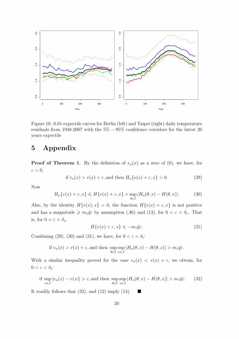
effects, we use the residuals after taking out such effects. We intend to construct
the confidence corridors for the 0.01 and 0.9-expectile curves for the residuals from
the fitted temperature model. We would like to investigate whether the performance
of the extreme values are same in different cities, further to analyze the risk factors
in different places.
The left part of the pictures describes the expectile curves for Berlin, and the
right part is for Taipei. In each figure, the thick black line depicts the average
expectile with the data from 1948 to 2007. The red line is the expectile for the
residuals from the model with the first 20 years temperature, i.e. we use the data
from 1948 to 1967. The 0.9 expectile for the second 20 years (1968-1987) residuals
is described by the green line, and the blue line stands for the expectile curve in the
latest 20 years (1988-2007). The dot lines are the 5% − 95% confidence corridors
corresponding to the expectile curve with the same color. Figures 4 − 7 describe the
0.9 expectile curve for the residuals from the the models for Berlin and Taipei, as
well as their corresponding confidence corridors. Obviously, the variance is higher
in winter-earlier summer both in Berlin and Taipei.
It is obvious to detect that the expectile curves in Berlin and Taipei are quite
different. Firstly, the variation of the temperature in Berlin is smaller than that of
Taipei. All the expectile curves cross with each other during the last 100 observations
for Berlin, and the variance in this period is smaller, seen from the expectile curves.
Moreover, all of them nearly locate in the corresponding three confidence corridors.
However, the performance of the temperature in Taipei is quite different. The
expectile curves for Taipei have similar trends for each 20 years. They have highest
volatilities in January, and lowest volatility in July. More interestingly, the expectile
curve for the latest 20 years does not locate in the confidence corridor constructed
using the data from the first 20 years and second 20 years, see Figure 4 and Figure 7.
Similarly, the expectile curve for the first 20 years does not locate in the confidence
corridor constructed by the latest 20 years.
Further, let us move to study the low expectile for the residuals from the models
for Berlin and Taipei. As we know, it is very hard to get the very low quantile curve,
due to the character of quantiles. However, it is not a problem for expectiles. One
can calculate very low or very high expectiles. Therefore, we also calculate the 0.01
expecitles for the residuals and their corresponding confidence corridors, which are
described in Figures 8 − 10. One can tell easily that the shapes of the 0.01 expectile
for Berlin and Taipei are different. It does not fluctuate a lot during the whole year
16
0 100 200 300
0.6
0.8
1.0
1.2
1.4
1.6
First expectile, and then average
Time
Re
sid
ua
ls
0 100 200 300
0.2
0.4
0.6
0.8
1.0
1.2
1.4
First expectile, and then average
Time
Re
sid
ua
ls
Figure 5: 0.9-expectile curves for Berlin (left) and Taipei (right) daily temperatureresiduals from 1948-2007 with the 5% − 95% confidence corridors for the first 20years expectile.
in Berlin, while the variation in Taipei is much bigger. However, all of these curves
both for Berlin and Taipei locate in their corresponding confidence corridors.
Obviously, one can say that the performance of the residuals are quite different
from Berlin and Taipei, after we take out the regular seasonal effect and AR effect,
especially for the high expectiles. Since the temperature can be influenced by the
human factors and other natural factors, which have been well documented in liter-
ature. We find the variation of the temperature in Taipei is more volatile. As one
interpretation, as we know in the last 60 years, Taiwan has been experiencing a fast
developing period, such as the industrial expansion, the burning of fossil fuel and
deforestation and other sectors, which would be an important factor to induce the
more volatility in the temperature of Taipei. However, Germany is well-developed
in this period, especially in Berlin, where there is no intensive industries. There-
fore, one may say the residuals reveals the influence of the human activities and we
conclude that the risk drivers for temperature are localized.
17
0 100 200 300
0.6
0.8
1.0
1.2
1.4
1.6
First expectile, and then average
Time
Re
sid
ua
ls
0 100 200 300
0.2
0.4
0.6
0.8
1.0
1.2
1.4
First expectile, and then average
TimeR
esi
du
als
Figure 6: 0.9-expectile curves for Berlin (left) and Taipei (right) daily temperatureresiduals from 1948-2007 with the 5%− 95% confidence corridors for the second 20years expectile.
0 100 200 300
0.6
0.8
1.0
1.2
1.4
1.6
First expectile, and then average
Time
Re
sid
ua
ls
0 100 200 300
0.2
0.4
0.6
0.8
1.0
1.2
1.4
First expectile, and then average
Time
Re
sid
ua
ls
Figure 7: 0.9-expectile curves for Berlin (left) and Taipei (right) daily temperatureresiduals from 1948-2007 with the 5% − 95% confidence corridors for the latest 20years expectile
18
0 100 200 300
−2.
0−
1.5
−1.
0−
0.5
0.0
First expectile, and then average
Time
Res
idua
ls
0 100 200 300
−2.
0−
1.5
−1.
0−
0.5
0.0
First expectile, and then average
Time
Res
idua
ls
Figure 8: 0.01-expectile curves for Berlin (left) and Taipei (right) daily temperatureresiduals from 1948-2007 with the 5% − 95% confidence corridors for the first 20years expectile
0 100 200 300
−2
.0−
1.5
−1
.0−
0.5
0.0
First expectile, and then average
Time
Re
sid
ua
ls
0 100 200 300
−2.
0−
1.5
−1.
0−
0.5
0.0
First expectile, and then average
Time
Res
idua
ls
Figure 9: 0.01-expectile curves for Berlin (left) and Taipei (right) daily temperatureresiduals from 1948-2007 with the 5%− 95% confidence corridors for the second 20years expectile
19
0 100 200 300
−2.
0−
1.5
−1.
0−
0.5
0.0
First expectile, and then average
Time
Res
idua
ls
0 100 200 300
−2.
0−
1.5
−1.
0−
0.5
0.0
First expectile, and then average
Time
Res
idua
ls
Figure 10: 0.01-expectile curves for Berlin (left) and Taipei (right) daily temperatureresiduals from 1948-2007 with the 5% − 95% confidence corridors for the latest 20years expectile
5 Appendix
Proof of Theorem 1. By the definition of vn(x) as a zero of (6), we have, for
ε > 0,
if vn(x) > v(x) + ε, and then Hn{v(x) + ε, x} > 0. (29)
We again estimate the left-hand side by Schwarz’s inequality and estimate each
factor separately,
E{Vn(x)− Vn(x1)}2 = (log n)(nh)−1 E[ n∑i=1
Ψn(x, x1, Xi, Yi) · I(|Yi| > an)
−E{Ψn(x, x1, Xi, Yi) · 1(|Yi| > an)}]2
,
where Ψn(x, x1, Xi, Yi) = ψ{Yi−v(x)}K{(x−Xi)/h}−ψ{Yi−v(x1)}K{(x1−X1)/h}.Since ψ, K are Lipschitz continuous except at one point and the expectation is taken
afterwards, it follows that
[E{Vn(x)− Vn(x1)}2]1/2
6 C7 · (log n)1/2h−3/2|x− x1| ·{∫{|y|>an}
fy(y)dy}1/2
.
If we apply the same estimation to Vn(x2)− Vn(x1) we finally have
E{|Vn(x)− Vn(x1)| · |Vn(x2)− Vn(x)|}
6 C27(log n)h−3|x− x1||x2 − x| ×
∫{|y|>an}
fy(y)dy
6 C ′ · |x2 − x1|2 since x ∈ [x1, x2] by (A3).
26
�
Lemma 10 Let λ(K) =∫K2(u)du and let {dn} be as in the theorem. Then
(2δ log n)1/2[‖Y3,n‖/{λ(K)}1/2 − dn]
has the same asymptotic distribution as
(2δ log n)1/2[‖Y4,n‖/{λ(K)}1/2 − dn].
PROOF. Y3,n(x) is a Gaussian process with
EY3,n(x) = 0
and covariance function
r3(x1, x2) = EY3,n(x1)Y3,n(x2)
= {g(x1)g(x2)}−1/2h−1
∫∫Γn
ψ2{y − v(x)}K{(x1 − x)/h}
×K{(x2 − x)/h}f(t, y)dtdy
= {g(x1)g(x2)}−1/2h−1
∫∫Γn
ψ2{y − v(x)}f(y|x)dyK{(x1 − x)/h}
×K{(x2 − x)/h}fX(x)dx
= {g(x1)g(x2)}−1/2h−1
∫g(x)K{(x1 − x)/h}K{(x2 − x)/h}dx
= r4(x1, x2)
where r4(x1, x2) is the covariance function of the Gaussian process Y4,n(x), which
proves the lemma. �
References
Benth, F., Benth, J., and Koekebakker, S. (2007). Putting a price on temperature.
Scandinavian Journal of Statistics, 34(4):746–767.
Bickel, P. and Rosenblatt, M. (1973). On some global measures of the deviation of
density function estimatiors. Annals of Statistics, 1:1071–1095.
Breckling, J. and Chambers, R. (1988). m-quantiles. Biometrika, 74(4):761–772.
27
Campbell, S. and Diebold, F. (2005). Weather forecasting for weather derivatives.
Journal of the American Statistical Association, 100:6–16.
Csorgo, S. and Hall, P. (1982). Upper and lower classes for triangular arrays.
Zeitschrift fur Wahrscheinlichkeitstheorie und verwandte Gebiete, 61:207–222.
Diebold, F. and Inoue, A. (2001). Long memory and regime switching. Journal of
Econometrics, 105:131–159.
Efron, B. (1991). Regression percentiles using asymmetric squared loss. Statistica
Sinica, 1:93–125.
Franke, J. and Mwita, P. (2003). Nonparametric estimates for conditional quantiles
of time series. Report in Wirtschaftsmathematik 87, University of Kaiserslautern.
Hardle, W. (1989). Asymptotic maximal deviation of M-smoothers. Journal of
Multivariate Analysis, 29:163–179.
Hardle, W., Janssen, P., and Serfling, R. (1988). Strong uniform consistency rates
for estimators of conditional functionals. Annals of Statistics, 16:1428–1429.
Hardle, W. and Luckhaus, S. (1984). Uniform consistency of a class of regression
function estimators. Annals of Statistics, 12:612–623.
Huber, P. (1981). Robust Statistics. Wiley, New York.
Johnston, G. (1982). Probabilities of maximal deviations of nonparametric regres-
sion function estimates. Journal of Multivariate Analysis, 12:402–414.
Jones, M. (1994). Expectiles and m-quantiles are quantiles. Statistics Probability
Letters, 20:149–153.
Kuan, C. M., Yeh, Y. H., and Hsu, Y. C. (2009). Assesing value at risk with
care, the conditional autoregressive expectile models. Journal of Econometrics,
150:261–270.
Newey, W. K. and Powell, J. L. (1987). Asymmetric least squares estimation and
testing. Econometrica, 55:819–847.
Parzen, M. (1962). On estimation of a probability density function and mode. Annals
of Mathematical Statistics, 32:1065–1076.
28
Rosenblatt, M. (1952). Remarks on a multivariate transformation. Annals of Math-
ematical Statistics, 23:470–472.
Schnabel, S. and Eilers, P. (2009a). An analysis of life expectancy and economic
production using expectile frontier zones. Demographic Research, 21:109–134.
Schnabel, S. and Eilers, P. (2009b). Optimal expectile smoothing. Computational
Statistics and Data Analysis, 53:4168–4177.
Taylor, J. (2008). Estimating value at risk and expected shortfall using expectiles.
Journal of Financial Econometrics, 6:231–252.
Tusnady, G. (1977). A remark on the approximation of the sample distribution
function in the multidimensional case. Periodica Mathematica Hungarica, 8:53–
55.
Yao, Q. and Tong, H. (1996). Asymmetric least squares regression estimation: a
nonparametric approach. Journal of Nonparametric Statistics, 6 (2-3):273–292.
Zhang, B. (1994). Nonparametric regression expectiles. Nonparametric Statistics,
3:255–275.
29
SFB 649 Discussion Paper Series 2011
For a complete list of Discussion Papers published by the SFB 649, please visit http://sfb649.wiwi.hu-berlin.de.
001 "Localising temperature risk" by Wolfgang Karl Härdle, Brenda López Cabrera, Ostap Okhrin and Weining Wang, January 2011.
002 "A Confidence Corridor for Sparse Longitudinal Data Curves" by Shuzhuan Zheng, Lijian Yang and Wolfgang Karl Härdle, January 2011.
003 "Mean Volatility Regressions" by Lu Lin, Feng Li, Lixing Zhu and Wolfgang Karl Härdle, January 2011.
004 "A Confidence Corridor for Expectile Functions" by Esra Akdeniz Duran, Mengmeng Guo and Wolfgang Karl Härdle, January 2011.
SFB 649, Ziegelstraße 13a, D-10117 Berlin http://sfb649.wiwi.hu-berlin.de
This research was supported by the Deutsche
Forschungsgemeinschaft through the SFB 649 "Economic Risk".


![Efficient Estimation in Expectile Regression Using ...[17] studied the sparse expectile regression under high dimensional settings where the penalty functions include the Lasso and](https://static.documents.pub/doc/80x56/5f029c6d7e708231d4052030/efficient-estimation-in-expectile-regression-using-17-studied-the-sparse-expectile.jpg)


