EDI042 – Error Control Coding(Kodningsteknik)

Chapter 4: Reed-Solomon Codes, Part IV

Michael Lentmaier

October 7, 2013

Berlekamp Massey Algorithm (BM)I The BM algorithm can be used to find the shortest linear

feedback shift register (LFSR) that generates the syndromeFour cases of RS Encoding

I Nonsystematic encoding based on g(X ).

v(X ) = u(X )g(X )

I Systematic encoding based on g(X ).

v(X ) = p(X ) + XN�Ku(X )

I Systematic encoding based on h(X ). Load u as the startingstate in a shift register with connection polynomial:

�(X ) = XKh(1X

)

I Nonsystematic encoding based on IDFT.

v0v1 . . . vN�1 = IDFT (u00 . . . 0u1u2 . . . uK�1)

Mats Cedervall, EiT, ECC, L11:12

Linear Feedback Shift Register, LFSR

· · ·

· · ·

· · ·+ +

vi�L vi�L+1 vi�1

��L ��L�1 ��1

v0, v1, . . . vi

The recursionThe LFSR, started at time 0, produces the output sequencev0v1 . . . vN�1, where the first v0v1 . . . vL�1 is the initial state of theshift register and vLvL+1 . . . vN�1 are produced according to therecursion

vi =L�

j=1

(��j)vi�j , i = L, L + 1, . . . , N � 1.

Mats Cedervall, EiT, ECC, L11:13

Linear Feedback Shift Register

DefinitionThe coefficients of the recursion or the multiplying constants in theLFSR can be used to define a connection polynomial �(X ):

�(X ) = 1 +L�

j=1

�jX j =��0

def= 1

�=

L�

j=0

�jX j .

Mats Cedervall, EiT, ECC, L11:14

Linear Feedback Shift Register

DefinitionThe linear complexity of the N-tuple v = v0v1 . . . vN�1, denotedLl or Ll (v), is the smallest value of L for which a recursion of theform

vi = �L�

j=1

�jvi�j , i = L, L + 1, . . . , N � 1

generates v from its first L components (starting state).The linear complexity of the allzero tuple is defined to be zero.

Mats Cedervall, EiT, ECC, L11:15

S1 S2 · · · SiSi�1Si�L Si�L+1

I The algorithm gets as input the values

S = (S1

,S2

, · · · ,SN�K)

I The output of the algorithm is an LFSR with connection weights

L1

,L2

, . . . ,LL ) L(X)

I The polynomial L(X) is the error location polynomial

Michael Lentmaier EDI042 – Error Control Coding: Chapter 4 29 / 39

Berlekamp Massey Algorithm (BM)

Decoding of RS Codes

Step 1

Let r0r1 . . . rN�1 be the received vector where r = v + e. We knowthat DFT(v) = V000 . . . 0VN�K+1 . . . VN�1 and thus

DFT(r) = DFT(v) + DFT(e) == R0E1E2 . . . EN�KRN�K+1 . . . RN�1.

ComputeE1E2 . . . EN�K from r .

Mats Cedervall, EiT, ECC, L11:20

Decoding of RS Codes

Step 2

Use the Berlekamp-Massey algorithm to find the error locatorpolynomial �(X ).

�(X ) = BM (E1E2 . . . EN�K )

Mats Cedervall, EiT, ECC, L11:21

The Berlekamp–Massey Algorithm

Yes

Yes

Startn � �1��1 � 1��2(X ) � 1��1(X ) � 1L � 0k � �1e � 1

n � n + 1�n � un �

L�

i=1(��i )un�i

e � e + 1

�n = 0

�n(X ) � �n�1(X ) � �n��1k Xe�k�1(X )

n < 2L

L � n + 1 � Lk � ne � 1

n un �n k e L �n(X )

-2 1-1 1 -1 1 0 1

Mats Cedervall, EiT, ECC, L11:22

Decoding of RS Codes

Step 3

Use E1, E2, . . . , EN�K and the error locator polynomial �(X ) toprocedure �EN�K+1, �EN�K+2, . . . , �EN�1, �E0.

Mats Cedervall, EiT, ECC, L11:23Use un = Sn+1

and run for n = 0, . . . ,N �K �1 ) L(X)

Michael Lentmaier EDI042 – Error Control Coding: Chapter 4 30 / 39

Alternative Error EvaluationI The shift register resulting from the BM algorithm can be used to

generate the remaining spectral error components

E1

,E2

, . . . ,EN�K ) ˆEN�K+1

, ˆEN�K+2

, . . . , ˆEN�1

, ˆE0

I This means that we can evaluate the errors by the inverse DFT

ˆe = IDFT�

ˆE0

,E1

,E2

, . . . ,EN�K , ˆEN�K+1

, . . . , ˆEN�1

�

I It is sufficient to compute the IDFT at the error locations j1

, . . . , jnthat follow from the connection polynomial L(X)

ejk = N�1

N�1

Âi=0

Ei a�jk i = N�1E�a�jk

�, k = 1, . . . ,n

I Attention: if the number of roots of L(X) is not equal to theLFSR length L = deg(L(X)), then we know that anuncorrectable error pattern occured (decoding failure)!

Michael Lentmaier EDI042 – Error Control Coding: Chapter 4 31 / 39

Overview of Algebraic Decoding1. Syndrome Computation

Sk = Ek = Rk = r�ak�, k = 1, . . . ,N �K

S(X) = S1

+S2

X + · · ·+SN�K XN�K�1

2. Error Location Polynomial

L(X) by solvingequation system

L(X) byBM algorithm

L(X) and T(X) byEuclidean algorithm

3. Error Positions: Chien Search

Find roots of L(X):L(X) =

�1�a j

1 X�· · ·�1�a jn X

�) j

1

, . . . , jn

4. Error EvaluationForney algorithm:

ejk =T(a�jk)L0(a�jk)

Computation of ˆE from L(X),ejk = N�1E

�a�jk

�

5. Error Correction: ˆv = r� ˆe

Michael Lentmaier EDI042 – Error Control Coding: Chapter 4 32 / 39

Extension Fields

Michael Lentmaier EDI042 – Error Control Coding: Chapter 4 33 / 39

Prime FieldsI Until now we have considered prime fields with integer elements

Fp = {0,1, . . . ,p�1}

where p is a prime numberI Multiplication and addition operations are performed modulo pI We have also seen that the non-zero elements of the field can be

represented as powers of a primitive element a of order p�1

Fp \0 = {1,a,a2,a3, . . . ,ap�2}

I Disadvantage: the number of elements in such fields isrestricted to prime numbers p

I The concept of extension fields can be used to create fields withq = pm elements for any prime number p and integer m � 1

I Extension fields of F2

with q = 2

m elements are mostattractive for implementation (binary vector representation)

Michael Lentmaier EDI042 – Error Control Coding: Chapter 4 34 / 39

Extension FieldsI Consider as example the field of real numbers RI The polynomial p(X) = X2 +1 could have up to two roots X = X

1

and X = X2

such that

p(X) = X2 +1 = (X �X1

)(X �X2

)

according to the fundamental theorem of algebra (see page 9)I Problem: there exist no solutions X

1

,X2

2 RI Solution: add an element j to the field R such that

p(j) = j2 +1 = 0 ) j2 = �1 ) j =p

�1 , X1

= j , X2

= �j

I We then define the field of complex numbers C by the elements

C = {a0

+a1

· j | a0

,a1

2 R}

I C is an extension field of R with polynomials as elementsI Addition and multiplication is performed modulo p(j)

Michael Lentmaier EDI042 – Error Control Coding: Chapter 4 35 / 39

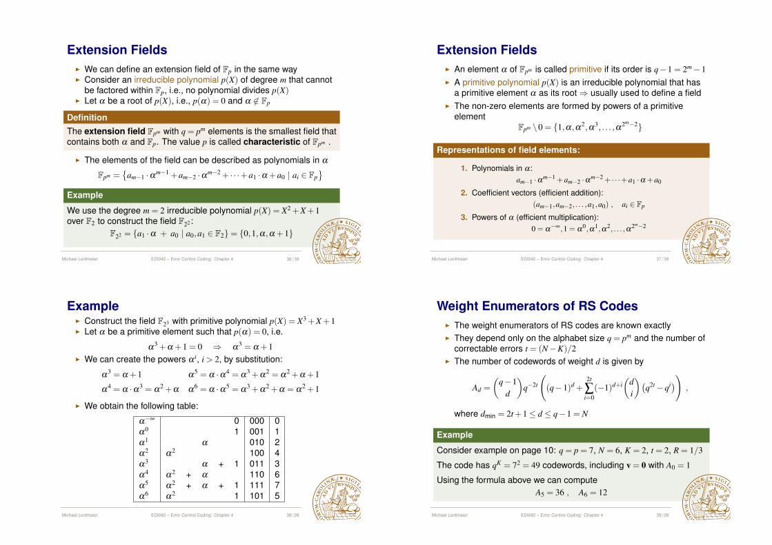
Extension FieldsI We can define an extension field of Fp in the same wayI Consider an irreducible polynomial p(X) of degree m that cannot

be factored within Fp, i.e., no polynomial divides p(X)I Let a be a root of p(X), i.e., p(a) = 0 and a 62 Fp

DefinitionThe extension field Fpm with q = pm elements is the smallest field thatcontains both a and Fp. The value p is called characteristic of Fpm .

I The elements of the field can be described as polynomials in aFpm =

�am�1

·am�1 +am�2

·am�2 + · · ·+a1

·a +a0

| ai 2 Fp

Example

We use the degree m = 2 irreducible polynomial p(X) = X2 +X +1

over F2

to construct the field F2

2

:F

2

2

= {a1

·a + a0

| a0

,a1

2 F2

} = {0,1,a,a +1}

Michael Lentmaier EDI042 – Error Control Coding: Chapter 4 36 / 39

Extension FieldsI An element a of Fpm is called primitive if its order is q�1 = 2

m �1

I A primitive polynomial p(X) is an irreducible polynomial that hasa primitive element a as its root ) usually used to define a field

I The non-zero elements are formed by powers of a primitiveelement

Fpm \0 = {1,a,a2,a3, . . . ,a2

m�2}

Representations of field elements:

1. Polynomials in a:am�1

·am�1 +am�2

·am�2 + · · ·+a1

·a +a0

2. Coefficient vectors (efficient addition):(am�1

,am�2

, . . . ,a1

,a0

) , ai 2 Fp

3. Powers of a (efficient multiplication):0 = a�•,1 = a0,a1,a2, . . . ,a2

m�2

Michael Lentmaier EDI042 – Error Control Coding: Chapter 4 37 / 39

ExampleI Construct the field F

2

3

with primitive polynomial p(X) = X3 +X +1

I Let a be a primitive element such that p(a) = 0, i.e.

a3 +a +1 = 0 ) a3 = a +1

I We can create the powers a i, i > 2, by substitution:

a3 = a +1 a5 = a ·a4 = a3 +a2 = a2 +a +1

a4 = a ·a3 = a2 +a a6 = a ·a5 = a3 +a2 +a = a2 +1

I We obtain the following table:

a�• 0 000 0a0 1 001 1a1 a 010 2a2 a2 100 4a3 a + 1 011 3a4 a2 + a 110 6a5 a2 + a + 1 111 7a6 a2 1 101 5

Michael Lentmaier EDI042 – Error Control Coding: Chapter 4 38 / 39

Weight Enumerators of RS CodesI The weight enumerators of RS codes are known exactlyI They depend only on the alphabet size q = pm and the number of

correctable errors t = (N �K)/2

I The number of codewords of weight d is given by

Ad =

✓q�1

d

◆q�2t

(q�1)d +

2t

Âi=0

(�1)d+i✓

di

◆�q2t �qi�

!,

where dmin = 2t +1 d q�1 = N

Example

Consider example on page 10: q = p = 7, N = 6, K = 2, t = 2, R = 1/3

The code has qK = 7

2 = 49 codewords, including v = 0 with A0

= 1

Using the formula above we can computeA

5

= 36 , A6

= 12

Michael Lentmaier EDI042 – Error Control Coding: Chapter 4 39 / 39