267
I. Opportunities in Michigan Wood Energy

I. Opportunities in Michigan Wood Energy

June 27, 2008Michigan Energy FairManistee Co. Fairgrounds – Onekama, MI
Presentation by: Jessica Simons
O P P O R T U N I T I E S I N

Presentation Overview
• What is Woody Biomass?• Why Wood?• Sources & Opportunities• Examples• Technical Issues• Helpful Resources

What is Woody Biomass?
• Biomass is simply any organic material –living or dead
• Woody biomass includes entire living & dead trees, brush, stems, logs, & other wood industrial residues

Biology 101 – How Trees GrowPhotosynthesis:
Carbon dioxide + water + energy (sunlight) = glucose/stored energy (mmm… sugar) + oxygen
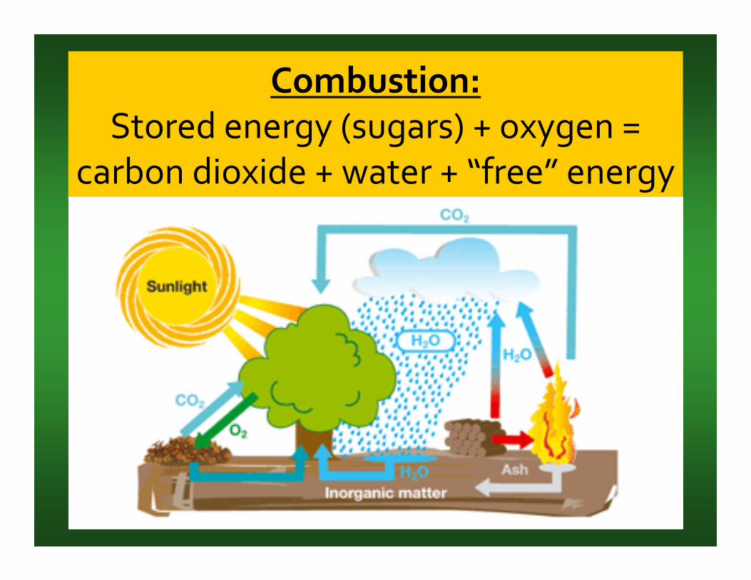
Combustion:Stored energy (sugars) + oxygen =
carbon dioxide + water + “free” energy

Presentation Overview
• What is Woody Biomass?• Why Wood?• Sources & Opportunities• Examples• Technical Issues• Helpful Resources

Wood is Good!
• Renewable• Local• Reliable• Sustainable• Affordable• Low carbon
emission• Minimal
ash• Very low
metals and sulfur
• Focus of presentation: larger‐scale wood boiler systems
for institutions and industry
• Can be used through new construction or boiler retrofit

“Compared to other bioenergy feedstocks, forestry sources have best outlook for feasibility and
environmental sustainability.”
Corn extensive cultivation, fertilization, & pest control
Woodwidely available, largely unused, low impact harvesting
From –Biomass, Biofuels and Bioenergy: Feedstock Opportunities in MIRobert E. Froese, Ph.D.; February 2007
Why Wood?
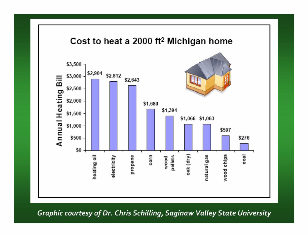
Graphic courtesy of Dr. Chris Schilling, Saginaw Valley State University

Presentation Overview
• What is Woody Biomass? • Why Wood?• Sources & Opportunities• Examples• Technical Issues• Helpful Resources

Best Sources for Wood?
• It all depends on where you are –
– Urban area? Look for urban sources – city tree removals, pallet recycling operations, clean crates and dunnage
– Rural area? Look to local forestland owners, forest products companies
• Always keep fuel quality (clean!) and dimensions(chip vs. ground) in mind when securing sources
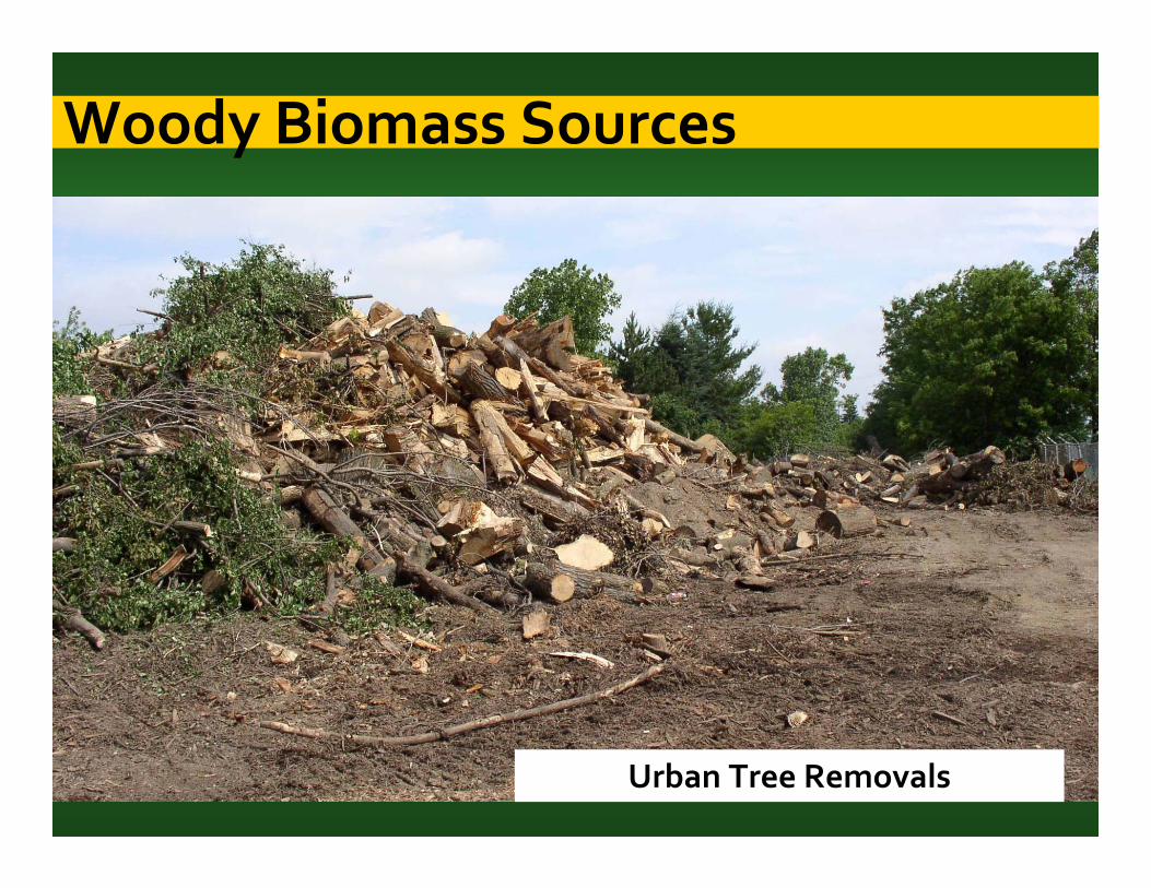
Woody Biomass Sources
Urban Tree Removals

Traditionally, communities pay large amounts for BOTH heating fuel and disposal of removed trees.
What happens to these figures if they get a wood boiler?
For example:
Imagine that a city pays –$25,000/yr to heat city hallAND $25,000/yr for wood disposal

Another source:EAB & Other Disasters
• At least 20 million dead and dying ash trees in Michigan
• Cities & residents face high costs for removal, disposal, & replanting

Industrial Residues
Woody Biomass Sources

2005SE Michigan Wood Residue
Inventory
2,600 companies7.5 million cu yds/yr
Disposal cost = $8.8 million28% landfilled
SE Michigan Urban Wood:both “green” & “brown”
So, how much wood is that, anyway?...
Enough to fill 354 football fields 10 ft deep!

Forest Slash & Thinnings
Woody Biomass Sources

Small‐diameter Timber
Woody Biomass Sources
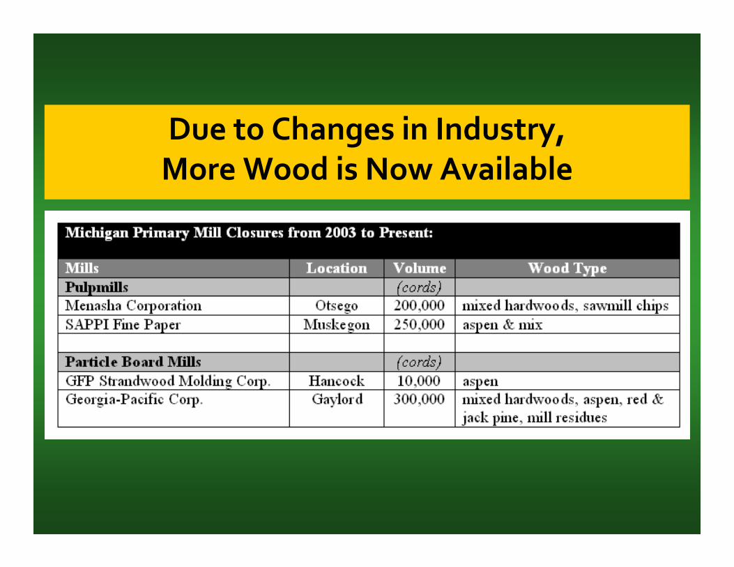
Due to Changes in Industry, More Wood is Now Available
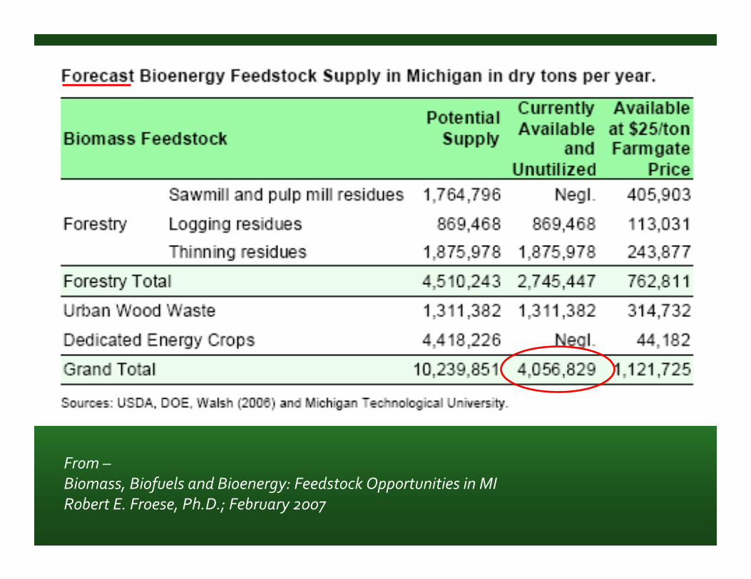
From –Biomass, Biofuels and Bioenergy: Feedstock Opportunities in MIRobert E. Froese, Ph.D.; February 2007
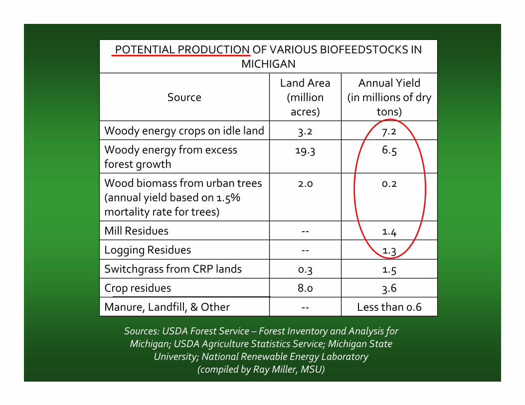
Less than 0.6‐‐Manure, Landfill, & Other
3.68.0Crop residues
1.50.3Switchgrass from CRP lands
1.3‐‐Logging Residues
1.4‐‐Mill Residues
0.22.0Wood biomass from urban trees (annual yield based on 1.5% mortality rate for trees)
6.519.3Woody energy from excess forest growth
7.23.2Woody energy crops on idle land
Annual Yield(in millions of dry
tons)
Land Area(million acres)
Source
POTENTIAL PRODUCTION OF VARIOUS BIOFEEDSTOCKS IN MICHIGAN
Sources: USDA Forest Service – Forest Inventory and Analysis for Michigan; USDA Agriculture Statistics Service; Michigan State
University; National Renewable Energy Laboratory (compiled by Ray Miller, MSU)

Presentation Overview
• What is Woody Biomass?• Why Wood?• Sources & Opportunities• Examples• Technical Issues• Helpful Resources

Pilot Program: Darby, MT Public Schools
Cost of wood chips (760 tons) = $ 18,170.00Cost of boiler operation & fuel study = $ 4,700.00Supplemental fuel oil = $ 1,935.002005‐2006 Actual Heating Costs = $ 24,805.00
Comparison of projected cost w/ fuel oil:Historic usage cost of fuel oil = $115,000.00(50,000 gal @ $2.30/gal)Estimated 2005‐2006 Cost Savings = $ 90,195.00
Example of Potential Wood Energy Savings
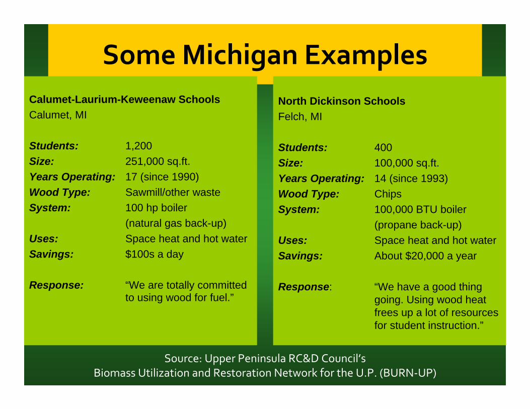
Some Michigan ExamplesCalumet-Laurium-Keweenaw Schools
Calumet, MI
Students: 1,200Size: 251,000 sq.ft.Years Operating: 17 (since 1990)Wood Type: Sawmill/other waste System: 100 hp boiler
(natural gas back-up)Uses: Space heat and hot waterSavings: $100s a day
Response: “We are totally committed to using wood for fuel.”
North Dickinson Schools
Felch, MI
Students: 400Size: 100,000 sq.ft. Years Operating: 14 (since 1993)Wood Type: ChipsSystem: 100,000 BTU boiler
(propane back-up)Uses: Space heat and hot waterSavings: About $20,000 a year
Response: “We have a good thing going. Using wood heat frees up a lot of resources for student instruction.”
Source: Upper Peninsula RC&D Council’s Biomass Utilization and Restoration Network for the U.P. (BURN‐UP)
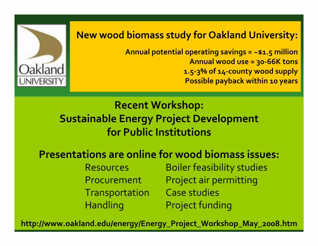
New wood biomass study for Oakland University:
Annual potential operating savings = ~$1.5 millionAnnual wood use = 30‐66K tons
1.5‐3% of 14‐county wood supplyPossible payback within 10 years
Recent Workshop:Sustainable Energy Project Development
for Public Institutions
Presentations are online for wood biomass issues:
http://www.oakland.edu/energy/Energy_Project_Workshop_May_2008.htm
ResourcesProcurementTransportationHandling
Boiler feasibility studiesProject air permittingCase studiesProject funding

…Projected figures from the Oakland University Study

Presentation Overview
• What is Woody Biomass?• Why Wood?• Sources & Opportunities • Examples• Technical Issues• Helpful Resources
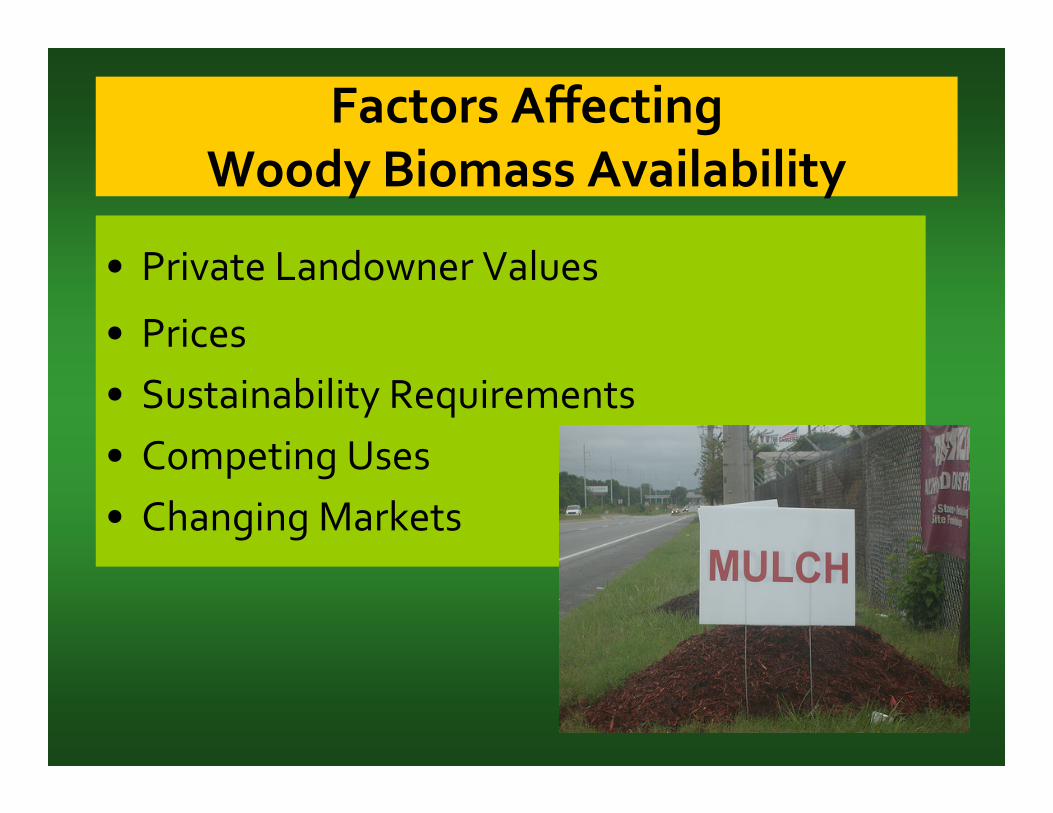
Factors Affecting Woody Biomass Availability
• Private Landowner Values
• Prices• Sustainability Requirements• Competing Uses• Changing Markets

Other Technical Issues
• Location • Separating residues from wastes• Landfills and tipping fees• Transportation• Harvesting• Collection• Processing – drying, chip size requirements• Maintaining fuel supply• Handling and maintenance

Larger‐scale woody biomass
energy production is NOT
the same as outdoor wood stoves
or open burning
Incomplete combustion = Pollution
But What About Air Quality?

“Over the course of a year, a large, wood‐heated high school
(150‐200K sq.ft.) may have the same particulate matter emissions as 4‐5
houses heated with wood stoves.”
Source:Biomass Energy Resource Center
http://www.biomasscenter.org/information/emissions.html

• Good fuel quality – no contaminated material
• Regular fuel inspections & equipment maintenance
• Tall stack height• Other equipment:
scrubbers & baghouses
Photo of CMU Boiler Plant by Jim Leidel
Measures to Support Clean Air

Presentation Overview
• What is Woody Biomass?• Why Wood?• Sources & Opportunities• Examples• Technical Issues• Helpful Resources

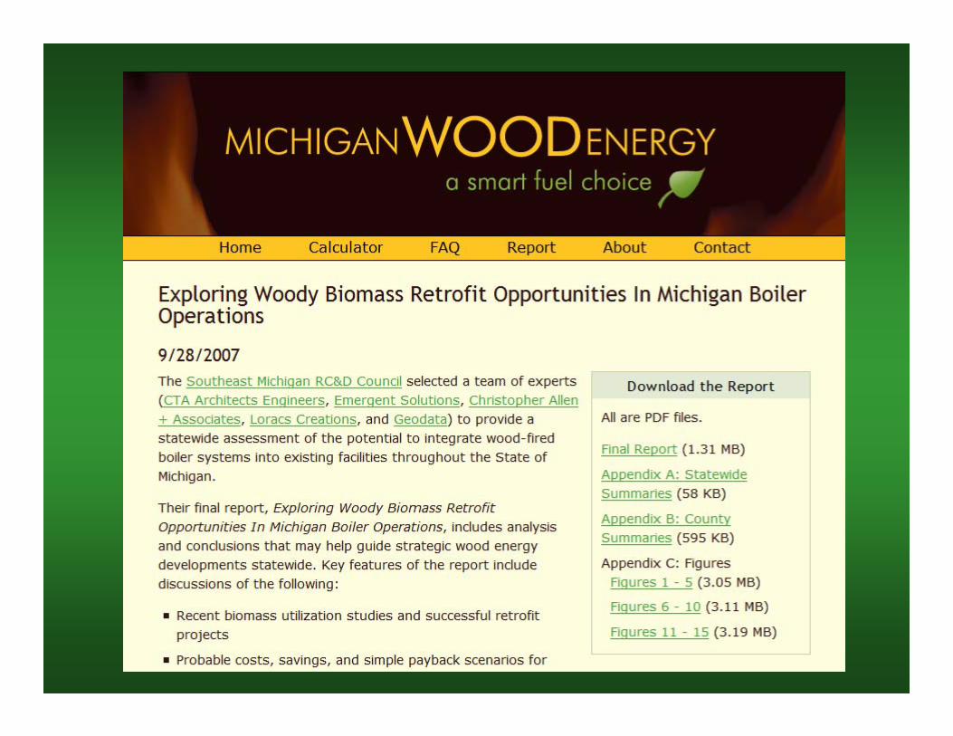
• Learn about wood energy options, view resources
• See report of 2,000 potential sites for wood energy in MI
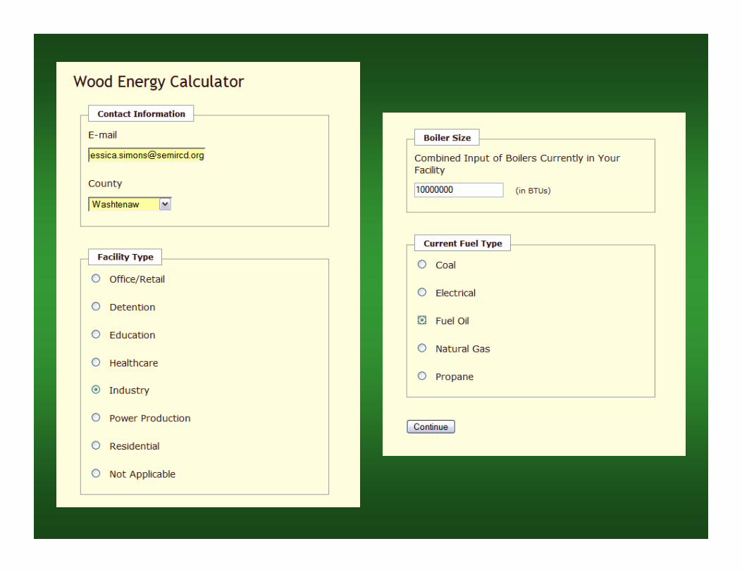
•Use calculator to estimate savings at your site
www.michiganwoodenergy.org


http://www.michigan.gov/documents/wood_energy_in_michigan‐‐final1_169999_7.pdf

Register on‐line at www.michigan.gov/deqworkshops,
click on “Upcoming DEQ Workshops,”
and scroll down to the Permit to Install series.
Confused About Permits?

http://www.upwoodybiomass.org/

Coming Soon…

Demonstration Project:City of Taylor
Heritage Park Petting Farm
Coming Soon…

These projects are made possible by generous grants and significant technical support from
Wood Education & Resource Center
Northeastern Area Rural Development Through
Forestry Program
Economic Action Program
And the Conservation Districts and governments that sponsor the Southeast
Michigan Resource Conservation &
Development Council

J. Potential Availability of Urban Wood Biomass in Michigan

Potential availability of urban wood biomass in Michigan:Implications for energy production, carbon sequestrationand sustainable forest management in the U.S.A.
David W. MacFarlane*
Department of Forestry, Michigan State University, 126 Natural Resources Building, East Lansing, MI 48824, USA
a r t i c l e i n f o
Article history:
Received 1 November 2007
Received in revised form
4 September 2008
Accepted 24 October 2008
Published online 28 November 2008
Keywords:
Wood biomass
Wood waste
Urban
Carbon sequestration
a b s t r a c t
Tree and wood biomass from urban areas is a potentially large, underutilized resource
viewed in the broader social context of biomass production and utilization. Here, data and
analysis from a regional study in a 13-county area of Michigan, U.S.A. are combined with
data and analysis from several other studies to examine this potential. The results suggest
that urban trees and wood waste offer a modest amount of biomass that could contribute
significantly more to regional and national bio-economies than it does at present. Better
utilization of biomass from urban trees and wood waste could offer new sources of locally
generated wood products and bio-based fuels for power and heat generation, reduce fossil
fuel consumption, reduce waste disposal costs and reduce pressure on forests. Although
wood biomass generally constitutes a ‘‘carbon-neutral’’ fuel, burning rather than burying
urban wood waste may not have a net positive effect on reducing atmospheric CO2 levels,
because it may reduce a significant long term carbon storage pool. Using urban wood
residues for wood products may provide the best balance of economic and environmental
values for utilization.
ª 2008 Elsevier Ltd. All rights reserved.
1. Introduction
Recent interest in developing biologically renewable fuel
sources has focused renewed attention on utilizing tree/
wood biomass for this purpose. In modern times, wood
makes up only 7% of global fuel sources, with an estimated
15% of energy used in developing nations and only about 2%
in developed nations [1], excluding some developed coun-
tries where substantial efforts have been made to use more
wood fuel (e.g., Sweden). Much of this wood comes from
forests, but a considerable amount also comes from what
the Food and Agricultural Organization of the United
Nations has termed ‘‘trees outside of forests’’ [2]. Generally,
the availability of wood from non-forest trees is not well
documented [1].
Wood from urban areas is one potentially large source of
biomass that appears currently underutilized. Wood biomass
from urban areas includes both wood waste generated when
wood products are damaged or outlive their usefulness [3] and
tree/wood biomass that is liberated when urban trees are
taken down or parts of woody vegetation are trimmed [4]. At
global and national scales, it appears that urban wood
biomass may offer a potentially large source of wood that
could be reused, burned for fuel or otherwise recycled [1,3,4].
However, some important questions remain regarding how
available urban wood biomass resources are and what are the
implications for trying to make use of them. In particular, it is
important that these questions be answered at local or
regional scales where wood utilization potential is most
practically assessed.
* Tel.: þ1 517 355 2399; fax: þ1 517 432 1143.E-mail address: [email protected]
Avai lab le at www.sc iencedi rect .com
ht tp : / /www. e lsev ier . com/ loca te / b i ombi oe
0961-9534/$ – see front matter ª 2008 Elsevier Ltd. All rights reserved.doi:10.1016/j.biombioe.2008.10.004
b i o m a s s a n d b i o e n e r g y 3 3 ( 2 0 0 9 ) 6 2 8 – 6 3 4

Here, new data and analysis on the potential availability of
biomass from urban trees in a 13-county area of Michigan,
U.S.A. is combined with existing data from several other
sources to examine the potential of urban tree removals and
other urban-generated sources of wood biomass to supply
locally generated bio-based fuels and primary and secondary
(recycled) wood products. The critical points of discussion
focus on the implications of urban wood utilization for energy
production, carbon sequestration and sustainable forest
management at the scale of regional and national economies.
2. Regional study: urban tree biomass insoutheastern lower Michigan
2.1. Study area
A regional assessment of standing urban saw timber in
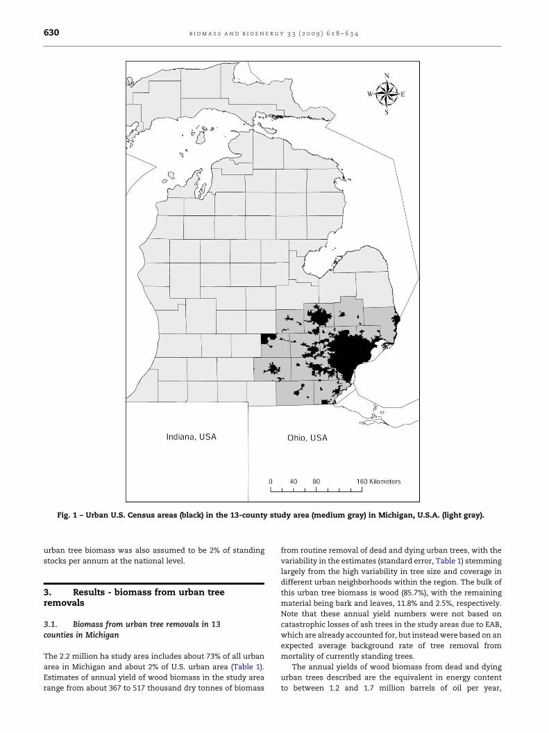
a 13-county region of southeastern lower Michigan (Fig. 1) was
recently completed [5]. The study area was comprised of
urban portions of the original 13 counties quarantined by the
Michigan Department of Agriculture due to the recent intro-
duction of the exotic wood-boring beetle, the emerald ash
borer (EAB, Agrilus plannipennis). This specific study region was
chosen because EAB has caused the death of estimated
millions of ash (Fraxinus spp.) there [6], which has focused
specific attention on the issue of better urban wood utiliza-
tion. This study area should be reasonably representative of
other similar urban areas in the Upper Midwest of the U.S.A.
2.2. Urban tree wood biomass estimation
Measurements of 1887 trees and stumps on 418 plots in 76
randomly selected urban neighborhoods in the study area [5]
were used to estimate urban tree biomass. Biomass equations
for urban-grown trees are not widely available, as they are for
forest-grown ones. Forest-derived biomass equations over-
estimate the biomass of urban (open grown) trees by about
25% leading to a rule of thumb of 0.8 units of urban biomass
per unit of biomass predicted for a forest-grown tree of
comparable size and species [7]. Using a general, composite
equation that combines the variety of species occurring in
urban areas together into a single predictive equation with
species-specific adjustments is considered superior to using
many different equations for different species derived from
different sources [7]. Thus, general whole tree above-ground
biomass models for forest-grown hardwoods and softwoods
[8,9] were adjusted to be 80% of predicted values to obtain
general whole tree biomass equations for urban hardwoods
and softwoods, respectively.
Whole tree biomass was portioned into bark and leaves via
urban tree leaf biomass equations [10] and species-specific
bark factors [11] and then into wood via subtraction. Wood
and bark biomass estimates were adjusted for individual
species with heavier or lighter than average wood, using
published values of wood and bark specific gravity for each
species [11]; an inflation/deflation factor was used that was
the ratio of the specific gravity of the species in question
divided by the average specific gravity for all of the species
considered. Only urban trees �20 cm diameter at breast
height (DBH) were measured in urban neighborhoods [5], so
the additional biomass contributed by smaller trees was
estimated by regression, contributing an additional 3%.
Hence, the final total dry wood biomass (metric tonnes, t)
estimates were the total amount for trees �20 cm (DBH) in
urban neighborhoods, inflated by 3% to account for the addi-
tional mass of dry wood per urban ha stored in smaller trees.
2.3. Scaling up individual tree estimates to the regionalscales
Tree biomass estimates (t ha�1) were scaled up to the regional
landscape scale by expanding neighborhood estimates to the
total land area estimated in an urban condition. Two common
methods are utilized for urban area estimation: (1) use polit-
ical boundaries such as city limits or census districts and
include any trees or forests in urban zones [12] or (2) use
classified satellite images to estimate urban areas remotely
[5,13]. Method 2 is overly conservative [5] and biased by
confusion between the conflicting tasks of identifying urban
areas on satellite images while simultaneously identifying
tree cover at the same location [13]. Urban treed areas for this
study were computed using a U.S. Census Bureau definition of
urban area [14] and percent urban tree cover for Michigan [12].
The ratio of urban tree biomass per % tree cover per ha was
used to scale up urban biomass to the census area. Urban tree
cover for the study area was previously too low due to use of
the satellite method [5] and so revised estimates for urban
sawn wood products available from urban trees were also
developed, scaled up in the same way as the new biomass
estimates.
2.4. Estimating potential annual yield from urban trees
In order to calculate the potential availability of urban wood
biomass on an annual basis, it was necessary to estimate the
rate at which urban trees would become available for utili-
zation. Most studies of potential wood biomass availability
focus on growth rates of different vegetation types [1]. Since
urban trees in the U.S. are not typically planted as crops or
harvested live, a reasonable estimate of availability was
derived from the mortality rate of urban trees; about 2% of the
standing volume of trees for this study area [5].
2.5. Estimating current utilization
Current utilization of wood residues was derived from
interviews with 1500 companies within the same 13-county
region [15].
2.6. National level estimates
Data from this study were combined with a national study of
tree cover and urban forest carbon sequestration [12] to
extrapolate regional results to the U.S.A.; carbon was con-
verted to total biomass assuming 0.5 t carbon per t biomass
and then to above ground biomass deducting the 21% of mass
in roots [12]. National utilization estimates were extrapolated
via data describing land filling of US wood [4]. Availability of
b i o m a s s a n d b i o e n e r g y 3 3 ( 2 0 0 9 ) 6 2 8 – 6 3 4 629
urban tree biomass was also assumed to be 2% of standing
stocks per annum at the national level.
3. Results - biomass from urban treeremovals
3.1. Biomass from urban tree removals in 13counties in Michigan
The 2.2 million ha study area includes about 73% of all urban
area in Michigan and about 2% of U.S. urban area (Table 1).
Estimates of annual yield of wood biomass in the study area
range from about 367 to 517 thousand dry tonnes of biomass
from routine removal of dead and dying urban trees, with the
variability in the estimates (standard error, Table 1) stemming
largely from the high variability in tree size and coverage in
different urban neighborhoods within the region. The bulk of
this urban tree biomass is wood (85.7%), with the remaining
material being bark and leaves, 11.8% and 2.5%, respectively.
Note that these annual yield numbers were not based on
catastrophic losses of ash trees in the study areas due to EAB,
which are already accounted for, but instead were based on an
expected average background rate of tree removal from
mortality of currently standing trees.
The annual yields of wood biomass from dead and dying
urban trees described are the equivalent in energy content
to between 1.2 and 1.7 million barrels of oil per year,
Fig. 1 – Urban U.S. Census areas (black) in the 13-county study area (medium gray) in Michigan, U.S.A. (light gray).
b i o m a s s a n d b i o e n e r g y 3 3 ( 2 0 0 9 ) 6 2 8 – 6 3 4630
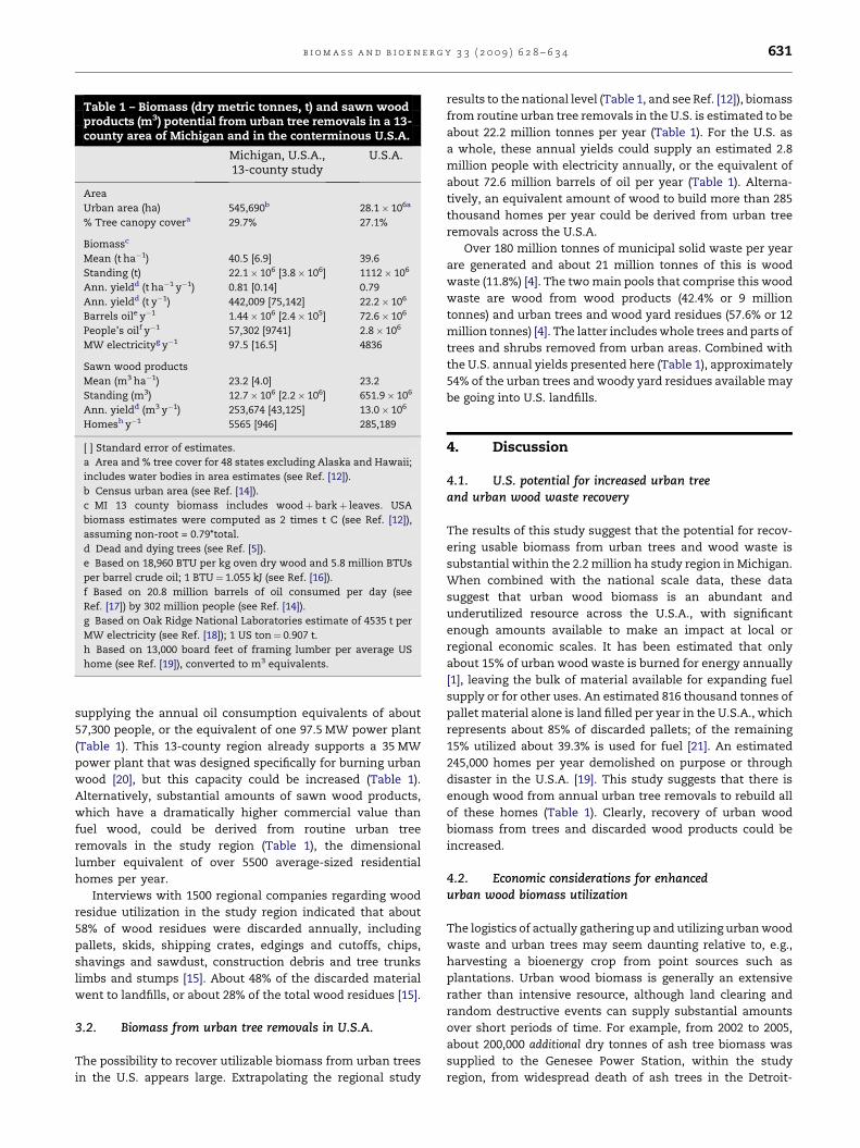
supplying the annual oil consumption equivalents of about
57,300 people, or the equivalent of one 97.5 MW power plant
(Table 1). This 13-county region already supports a 35 MW
power plant that was designed specifically for burning urban
wood [20], but this capacity could be increased (Table 1).
Alternatively, substantial amounts of sawn wood products,
which have a dramatically higher commercial value than
fuel wood, could be derived from routine urban tree
removals in the study region (Table 1), the dimensional
lumber equivalent of over 5500 average-sized residential
homes per year.
Interviews with 1500 regional companies regarding wood
residue utilization in the study region indicated that about
58% of wood residues were discarded annually, including
pallets, skids, shipping crates, edgings and cutoffs, chips,
shavings and sawdust, construction debris and tree trunks
limbs and stumps [15]. About 48% of the discarded material
went to landfills, or about 28% of the total wood residues [15].
3.2. Biomass from urban tree removals in U.S.A.
The possibility to recover utilizable biomass from urban trees
in the U.S. appears large. Extrapolating the regional study
results to the national level (Table 1, and see Ref. [12]), biomass
from routine urban tree removals in the U.S. is estimated to be
about 22.2 million tonnes per year (Table 1). For the U.S. as
a whole, these annual yields could supply an estimated 2.8
million people with electricity annually, or the equivalent of
about 72.6 million barrels of oil per year (Table 1). Alterna-
tively, an equivalent amount of wood to build more than 285
thousand homes per year could be derived from urban tree
removals across the U.S.A.
Over 180 million tonnes of municipal solid waste per year
are generated and about 21 million tonnes of this is wood
waste (11.8%) [4]. The two main pools that comprise this wood
waste are wood from wood products (42.4% or 9 million
tonnes) and urban trees and wood yard residues (57.6% or 12
million tonnes) [4]. The latter includes whole trees and parts of
trees and shrubs removed from urban areas. Combined with
the U.S. annual yields presented here (Table 1), approximately
54% of the urban trees and woody yard residues available may
be going into U.S. landfills.
4. Discussion
4.1. U.S. potential for increased urban treeand urban wood waste recovery
The results of this study suggest that the potential for recov-
ering usable biomass from urban trees and wood waste is
substantial within the 2.2 million ha study region in Michigan.
When combined with the national scale data, these data
suggest that urban wood biomass is an abundant and
underutilized resource across the U.S.A., with significant
enough amounts available to make an impact at local or
regional economic scales. It has been estimated that only
about 15% of urban wood waste is burned for energy annually
[1], leaving the bulk of material available for expanding fuel
supply or for other uses. An estimated 816 thousand tonnes of
pallet material alone is land filled per year in the U.S.A., which
represents about 85% of discarded pallets; of the remaining
15% utilized about 39.3% is used for fuel [21]. An estimated
245,000 homes per year demolished on purpose or through
disaster in the U.S.A. [19]. This study suggests that there is
enough wood from annual urban tree removals to rebuild all
of these homes (Table 1). Clearly, recovery of urban wood
biomass from trees and discarded wood products could be
increased.
4.2. Economic considerations for enhancedurban wood biomass utilization
The logistics of actually gathering up and utilizing urban wood
waste and urban trees may seem daunting relative to, e.g.,
harvesting a bioenergy crop from point sources such as
plantations. Urban wood biomass is generally an extensive
rather than intensive resource, although land clearing and
random destructive events can supply substantial amounts
over short periods of time. For example, from 2002 to 2005,
about 200,000 additional dry tonnes of ash tree biomass was
supplied to the Genesee Power Station, within the study
region, from widespread death of ash trees in the Detroit-
Table 1 – Biomass (dry metric tonnes, t) and sawn woodproducts (m3) potential from urban tree removals in a 13-county area of Michigan and in the conterminous U.S.A.
Michigan, U.S.A.,13-county study
U.S.A.
Area
Urban area (ha) 545,690b 28.1� 106a
% Tree canopy covera 29.7% 27.1%
Biomassc
Mean (t ha�1) 40.5 [6.9] 39.6
Standing (t) 22.1� 106 [3.8� 106] 1112� 106
Ann. yieldd (t ha�1 y�1) 0.81 [0.14] 0.79
Ann. yieldd (t y�1) 442,009 [75,142] 22.2� 106
Barrels oile y�1 1.44� 106 [2.4� 105] 72.6� 106
People’s oilf y�1 57,302 [9741] 2.8� 106
MW electricityg y�1 97.5 [16.5] 4836
Sawn wood products
Mean (m3 ha�1) 23.2 [4.0] 23.2
Standing (m3) 12.7� 106 [2.2� 106] 651.9� 106
Ann. yieldd (m3 y�1) 253,674 [43,125] 13.0� 106
Homesh y�1 5565 [946] 285,189
[ ] Standard error of estimates.
a Area and % tree cover for 48 states excluding Alaska and Hawaii;
includes water bodies in area estimates (see Ref. [12]).
b Census urban area (see Ref. [14]).
c MI 13 county biomass includes woodþ barkþ leaves. USA
biomass estimates were computed as 2 times t C (see Ref. [12]),
assuming non-root = 0.79*total.
d Dead and dying trees (see Ref. [5]).
e Based on 18,960 BTU per kg oven dry wood and 5.8 million BTUs
per barrel crude oil; 1 BTU¼ 1.055 kJ (see Ref. [16]).
f Based on 20.8 million barrels of oil consumed per day (see
Ref. [17]) by 302 million people (see Ref. [14]).
g Based on Oak Ridge National Laboratories estimate of 4535 t per
MW electricity (see Ref. [18]); 1 US ton¼ 0.907 t.
h Based on 13,000 board feet of framing lumber per average US
home (see Ref. [19]), converted to m3 equivalents.
b i o m a s s a n d b i o e n e r g y 3 3 ( 2 0 0 9 ) 6 2 8 – 6 3 4 631
Metropolitan area, providing an additional 22.4 MW of elec-
tricity [20]. However, the latter was orchestrated in part, via
government incentives to sanitize infested trees [20]. Thus,
under typical conditions, incentives in the form of avoided
costs or direct gains may be necessary to make collecting
urban wood waste attractive. For example, a nationwide
average cost reduction of about $9 per tonne was reported in
the U.S.A. in 1995, if pallets were simply disposed of at a wood
waste processing facility ($26 per tonne) instead of land filling
as is ($35 per tonne) [21].
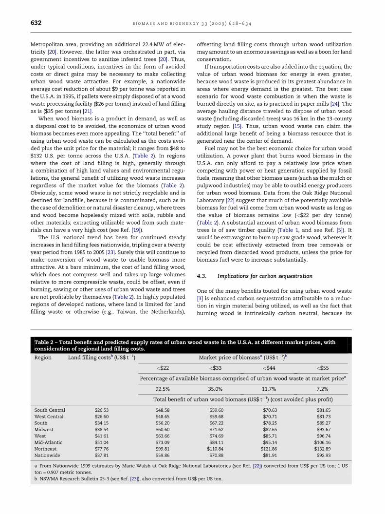
When wood biomass is a product in demand, as well as
a disposal cost to be avoided, the economics of urban wood
biomass becomes even more appealing. The ‘‘total benefit’’ of
using urban wood waste can be calculated as the costs avoi-
ded plus the unit price for the material; it ranges from $48 to
$132 U.S. per tonne across the U.S.A. (Table 2). In regions
where the cost of land filling is high, generally through
a combination of high land values and environmental regu-
lations, the general benefit of utilizing wood waste increases
regardless of the market value for the biomass (Table 2).
Obviously, some wood waste is not strictly recyclable and is
destined for landfills, because it is contaminated, such as in
the case of demolition or natural disaster cleanup, where trees
and wood become hopelessly mixed with soils, rubble and
other materials; extracting utilizable wood from such mate-
rials can have a very high cost (see Ref. [19]).
The U.S. national trend has been for continued steady
increases in land filling fees nationwide, tripling over a twenty
year period from 1985 to 2005 [23]. Surely this will continue to
make conversion of wood waste to usable biomass more
attractive. At a bare minimum, the cost of land filling wood,
which does not compress well and takes up large volumes
relative to more compressible waste, could be offset, even if
burning, sawing or other uses of urban wood waste and trees
are not profitable by themselves (Table 2). In highly populated
regions of developed nations, where land is limited for land
filling waste or otherwise (e.g., Taiwan, the Netherlands),
offsetting land filling costs through urban wood utilization
may amount to an enormous savings as well as a boon for land
conservation.
If transportation costs are also added into the equation, the
value of urban wood biomass for energy is even greater,
because wood waste is produced in its greatest abundance in
areas where energy demand is the greatest. The best case
scenario for wood waste combustion is when the waste is
burned directly on site, as is practiced in paper mills [24]. The
average hauling distance traveled to dispose of urban wood
waste (including discarded trees) was 16 km in the 13-county
study region [15]. Thus, urban wood waste can claim the
additional large benefit of being a biomass resource that is
generated near the center of demand.
Fuel may not be the best economic choice for urban wood
utilization. A power plant that burns wood biomass in the
U.S.A. can only afford to pay a relatively low price when
competing with power or heat generation supplied by fossil
fuels, meaning that other biomass users (such as the mulch or
pulpwood industries) may be able to outbid energy producers
for urban wood biomass. Data from the Oak Ridge National
Laboratory [22] suggest that much of the potentially available
biomass for fuel will come from urban wood waste as long as
the value of biomass remains low (<$22 per dry tonne)
(Table 2). A substantial amount of urban wood biomass from
trees is of saw timber quality (Table 1, and see Ref. [5]). It
would be extravagant to burn up saw grade wood, wherever it
could be cost effectively extracted from tree removals or
recycled from discarded wood products, unless the price for
biomass fuel were to increase substantially.
4.3. Implications for carbon sequestration
One of the many benefits touted for using urban wood waste
[3] is enhanced carbon sequestration attributable to a reduc-
tion in virgin material being utilized, as well as the fact that
burning wood is intrinsically carbon neutral, because its
Table 2 – Total benefit and predicted supply rates of urban wood waste in the U.S.A. at different market prices, withconsideration of regional land filling costs.
Region Land filling costsb (US$ t�1) Market price of biomassa (US$ t�1)b
<$22 <$33 <$44 <$55
Percentage of available biomass comprised of urban wood waste at market pricea
92.5% 35.0% 11.7% 7.2%
Total benefit of urban wood biomass (US$ t�1) (cost avoided plus profit)
South Central $26.53 $48.58 $59.60 $70.63 $81.65
West Central $26.60 $48.65 $59.68 $70.71 $81.73
South $34.15 $56.20 $67.22 $78.25 $89.27
Midwest $38.54 $60.60 $71.62 $82.65 $93.67
West $41.61 $63.66 $74.69 $85.71 $96.74
Mid-Atlantic $51.04 $73.09 $84.11 $95.14 $106.16
Northeast $77.76 $99.81 $110.84 $121.86 $132.89
Nationwide $37.81 $59.86 $70.88 $81.91 $92.93
a From Nationwide 1999 estimates by Marie Walsh at Oak Ridge National Laboratories (see Ref. [22]) converted from US$ per US ton; 1 US
ton¼ 0.907 metric tonnes.
b NSWMA Research Bulletin 05-3 (see Ref. [23]), also converted from US$ per US ton.
b i o m a s s a n d b i o e n e r g y 3 3 ( 2 0 0 9 ) 6 2 8 – 6 3 4632
ultimate energy source is solar. While all wood-derived sour-
ces are superior in this regard to fossil fuels, consumption of
wood from different sources will have a different impact on
net CO2 sequestration, because the life expectancy of wood
carbon (i.e., decomposition rate) is not equal for wood in all of
its forms [25].
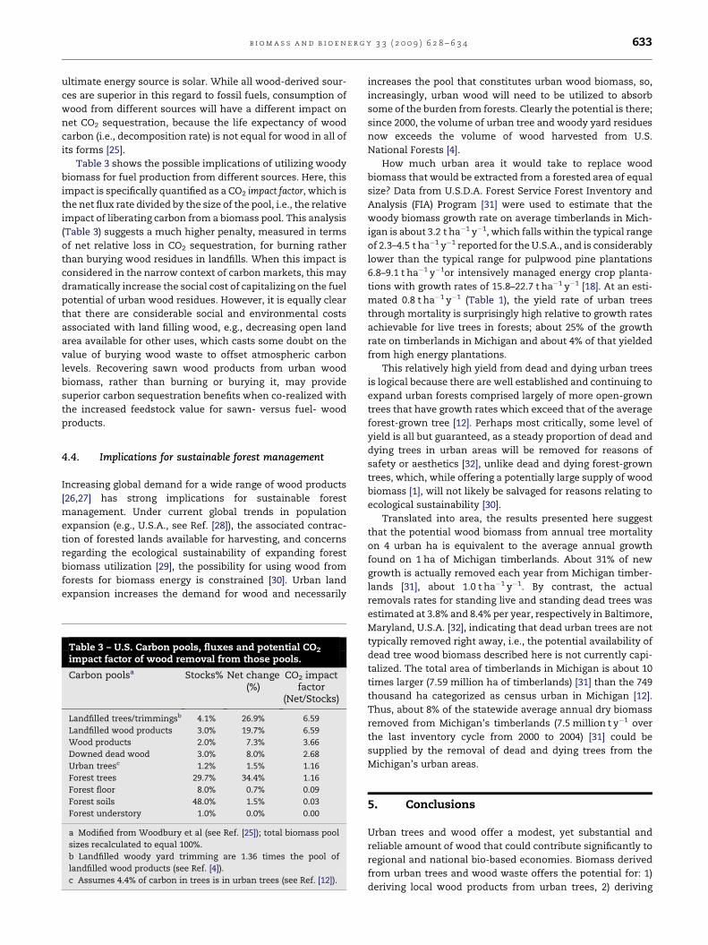
Table 3 shows the possible implications of utilizing woody
biomass for fuel production from different sources. Here, this
impact is specifically quantified as a CO2 impact factor, which is
the net flux rate divided by the size of the pool, i.e., the relative
impact of liberating carbon from a biomass pool. This analysis
(Table 3) suggests a much higher penalty, measured in terms
of net relative loss in CO2 sequestration, for burning rather
than burying wood residues in landfills. When this impact is
considered in the narrow context of carbon markets, this may
dramatically increase the social cost of capitalizing on the fuel
potential of urban wood residues. However, it is equally clear
that there are considerable social and environmental costs
associated with land filling wood, e.g., decreasing open land
area available for other uses, which casts some doubt on the
value of burying wood waste to offset atmospheric carbon
levels. Recovering sawn wood products from urban wood
biomass, rather than burning or burying it, may provide
superior carbon sequestration benefits when co-realized with
the increased feedstock value for sawn- versus fuel- wood
products.
4.4. Implications for sustainable forest management
Increasing global demand for a wide range of wood products
[26,27] has strong implications for sustainable forest
management. Under current global trends in population
expansion (e.g., U.S.A., see Ref. [28]), the associated contrac-
tion of forested lands available for harvesting, and concerns
regarding the ecological sustainability of expanding forest
biomass utilization [29], the possibility for using wood from
forests for biomass energy is constrained [30]. Urban land
expansion increases the demand for wood and necessarily
increases the pool that constitutes urban wood biomass, so,
increasingly, urban wood will need to be utilized to absorb
some of the burden from forests. Clearly the potential is there;
since 2000, the volume of urban tree and woody yard residues
now exceeds the volume of wood harvested from U.S.
National Forests [4].
How much urban area it would take to replace wood
biomass that would be extracted from a forested area of equal
size? Data from U.S.D.A. Forest Service Forest Inventory and
Analysis (FIA) Program [31] were used to estimate that the
woody biomass growth rate on average timberlands in Mich-
igan is about 3.2 t ha�1 y�1, which falls within the typical range
of 2.3–4.5 t ha�1 y�1 reported for the U.S.A., and is considerably
lower than the typical range for pulpwood pine plantations
6.8–9.1 t ha�1 y�1or intensively managed energy crop planta-
tions with growth rates of 15.8–22.7 t ha�1 y�1 [18]. At an esti-
mated 0.8 t ha�1 y�1 (Table 1), the yield rate of urban trees
through mortality is surprisingly high relative to growth rates
achievable for live trees in forests; about 25% of the growth
rate on timberlands in Michigan and about 4% of that yielded
from high energy plantations.
This relatively high yield from dead and dying urban trees
is logical because there are well established and continuing to
expand urban forests comprised largely of more open-grown
trees that have growth rates which exceed that of the average
forest-grown tree [12]. Perhaps most critically, some level of
yield is all but guaranteed, as a steady proportion of dead and
dying trees in urban areas will be removed for reasons of
safety or aesthetics [32], unlike dead and dying forest-grown
trees, which, while offering a potentially large supply of wood
biomass [1], will not likely be salvaged for reasons relating to
ecological sustainability [30].
Translated into area, the results presented here suggest
that the potential wood biomass from annual tree mortality
on 4 urban ha is equivalent to the average annual growth
found on 1 ha of Michigan timberlands. About 31% of new
growth is actually removed each year from Michigan timber-
lands [31], about 1.0 t ha�1 y�1. By contrast, the actual
removals rates for standing live and standing dead trees was
estimated at 3.8% and 8.4% per year, respectively in Baltimore,
Maryland, U.S.A. [32], indicating that dead urban trees are not
typically removed right away, i.e., the potential availability of
dead tree wood biomass described here is not currently capi-
talized. The total area of timberlands in Michigan is about 10
times larger (7.59 million ha of timberlands) [31] than the 749
thousand ha categorized as census urban in Michigan [12].
Thus, about 8% of the statewide average annual dry biomass
removed from Michigan’s timberlands (7.5 million t y�1 over
the last inventory cycle from 2000 to 2004) [31] could be
supplied by the removal of dead and dying trees from the
Michigan’s urban areas.
5. Conclusions
Urban trees and wood offer a modest, yet substantial and
reliable amount of wood that could contribute significantly to
regional and national bio-based economies. Biomass derived
from urban trees and wood waste offers the potential for: 1)
deriving local wood products from urban trees, 2) deriving
Table 3 – U.S. Carbon pools, fluxes and potential CO2
impact factor of wood removal from those pools.
Carbon poolsa Stocks% Net change(%)
CO2 impactfactor
(Net/Stocks)
Landfilled trees/trimmingsb 4.1% 26.9% 6.59
Landfilled wood products 3.0% 19.7% 6.59
Wood products 2.0% 7.3% 3.66
Downed dead wood 3.0% 8.0% 2.68
Urban treesc 1.2% 1.5% 1.16
Forest trees 29.7% 34.4% 1.16
Forest floor 8.0% 0.7% 0.09
Forest soils 48.0% 1.5% 0.03
Forest understory 1.0% 0.0% 0.00
a Modified from Woodbury et al (see Ref. [25]); total biomass pool
sizes recalculated to equal 100%.
b Landfilled woody yard trimming are 1.36 times the pool of
landfilled wood products (see Ref. [4]).
c Assumes 4.4% of carbon in trees is in urban trees (see Ref. [12]).
b i o m a s s a n d b i o e n e r g y 3 3 ( 2 0 0 9 ) 6 2 8 – 6 3 4 633

locally generated fuel sources for power and heat generation,
3) reducing fossil fuel consumption, 4) reducing waste
disposal costs, and 5) reducing pressure on forests.
Although wood biomass generally constitutes a ‘‘carbon-
neutral’’ fuel, burning rather than burying urban wood waste
may not have a net positive effect on reducing atmospheric
CO2 levels, because it may reduce a significant long term
carbon storage pool. Using urban wood residues for wood
products may provide the best balance of economic and
environmental values for utilization.
Acknowledgements
The author would like to thank the Michigan Agricultural
Experiment Station and the Southeast Michigan Resource
Conservation and Development Council for funding this
research. The author would also like to thank E.P. Barrett for
useful comments on this manuscript.
r e f e r e n c e s
[1] Mead DJ. Forest for energy and the role of planted trees.Critical Reviews in Plant Sciences 2005;24:407–21.
[2] FAO. Trees outside of forests. In: Bellfontaine R, Petit S, Pain-Orcet M, Deletorte P, Bertault JG, editors. FAO conservationguide 35. Rome: Food and Agricultural Organization of theUnited Nations; 2002.
[3] Solid Waste Association of North America. Successfulapproaches to recycling urban wood waste. Gen. Tech.Report. FPL-GTR-133. Madison, WI: USDA Forest Service,Forest Products Laboratory; 2002. p. 20.
[4] McKeever DB, Skog KE. Urban tree and wood yard residuesanother wood resource. Research note: FPL-RN-0290.Madison, WI: USDA Forest Service, Forest ProductsLaboratory; 2003. p. 4.
[5] MacFarlane DW. Quantifying urban saw timber abundanceand quality in southeastern lower Michigan, U.S.A.Arboriculture and Urban Forestry 2007;33(4):253–63.
[6] Poland TM, McCullough DG. Emerald ash borer: invasion ofthe urban forest and the threat to North America’s ashresource. Journal of Forestry 2006;104(3):118–24.
[7] Nowak DJ, Crane DE, Stevens JC, Ibarra M. Brooklyn’s urbanforest. General Technical report, GTR-NE-290. NewtownSquare, PA: USDA Forest Service, North Central ResearchStation; 2001. p. 107.
[8] Monteith DB. Whole-tree weight tables for New York.Syracuse University of New York; 1979. AFRI Res. Rep. 40. p. 67.
[9] Tritton LM, Hornbeck JW. Biomass equations for major treespecies of the northeast. U.S.A.D.A. Forest Service,Northeastern Forest Experiment Station; 1982. GTR NE-69.
[10] Nowak DJ. Estimating leaf area and leaf biomass of open-grown deciduous urban trees. Forest Science 1996;42(4):504–7.
[11] Smith WB. Factors and equations to estimate forest biomass inthenorthcentral region.U.S.A.D.A. ForestService, NorthCentralForest Experiment Station; 1985. Research Paper NC-268.
[12] Nowak DJ, CraneDE.Carbon storageand sequestration by urbantrees in the U.S.A. Environmental Pollution 2002;166:381–9.
[13] Fang S, Gertner G, Wang G, Anderson A. The implication ofmisclassification in land use maps in the prediction oflandscape dynamics. Landscape Ecology 2006;21:233–42.
[14] Available from: <http://www.census.gov/geo/www/ua/ua_bdfile.html> [accessed 27.08.08].
[15] Sherrill SB, MacFarlane DW. Measures of wood resources inlower Michigan: wood residues and the saw timber contentof urban forests. Technical report to the southeast Michiganresource conservation and development council and the U.S.D.A. forest service; May 2007. p. 178.
[16] Available from: <http://bioenergy.ornl.gov/papers/misc/energy_conv.html> [accessed 27.08.08].
[17] Available from: <http://www.eia.doe.gov/basics/quickoil.html> [accessed 27.08.08].
[18] Available from: <http://bioenergy.ornl.gov/resourcedata/powerandwood.html> [accessed 27.08.08].
[19] Falk B. Wood-framed building deconstruction a source oflumber for construction? Wood Products Journal 2002;52(3):8–15.
[20] Edward P. Barrett, Manager. Mid-Michigan recycling, pers.com.
[21] Bush RJ, Araman PA. Construction & demolition landfills andwood pallets - what’s happening in the U.S.A. PalletEnterprise; March 1997. p. 27–31.
[22] Available from: <http://bioenergy.ornl.gov/main.aspx>[accessed 27.08.08].
[23] Repa EW. NSWMA’s 2005 tip fee survey. NSWMA ResearchBulletin 05-3. Washington, D.C.: National Solid WasteManagement Association; March 2005. p. 3.
[24] Singer JG. Combustion fossil power. A reference book on fuelburning and steam generation. Windsor, Connecticut:Combustion Engineering, Inc.; 1993. p. 140.
[25] Woodbury PB, Smith JE, Heath LS. Carbon sequestration inthe U.S.A. forest sector from 1990 to 2010. Forest Ecology andManagement 2007;241:14–27.
[26] Whiteman A, Brown C. Modelling global forest productssupply and demand: recent results from FAO and theirpotential implications for New Zealand. New Zealand Journalof Forestry 2000;44(4):6–9.
[27] Zhu S, Buongiorno J, Brooks DJ. Global effects of acceleratedtariff liberalization in the forest products sector to 2010.Research paper: PNW-RP-534. Corvallis, OR: USDA ForestService, Forest Science Laboratory; 2002. p. 50.
[28] Nowak DJ, Walton JT, Dwyer JF, Kaya LG, Myeong S. Theincreasing influence of urban environments on U.S.A. forestmanagement. Journal of Forestry 2005;103(8):377–82.
[29] Egnell G, Valinger E. Survival, growth, and growth allocationof planted scots pine trees after different levels of biomassremoval in clear-felling. Forest Ecology and Management2003;177:65–74.
[30] Raison RJ. Opportunities and impediments to expansion offorest bioenergy in Australia. Biomass & Bioenergy 2006;30:1021–4.
[31] USDA forest service forest inventory and analysis data,Michigan 2004, complete panel, <http://fia.fs.fed.us/>[accessed 17.9.07].
[32] Nowak DJ, Kuroda M, Crane DE. Tree morality rates and treepopulation projections in Baltimore, Maryland, U.S.A. UrbanForestry & Urban Greening 2004;2:139–47.
b i o m a s s a n d b i o e n e r g y 3 3 ( 2 0 0 9 ) 6 2 8 – 6 3 4634

K. Quantifying Urban Saw Timber Abundance and Quality in Southeastern Lower Michigan
Quantifying Urban Saw Timber Abundance and Qualityin Southeastern Lower Michigan, U.S.
David W. MacFarlane
Abstract. There is a growing need for society to use resources efficiently, including effective use of dead and dying treesin urban areas. Harvesting saw timber from urban trees is a high-end use, but currently, much urban wood ends up inlandfills or is used for wood chips or biomass fuel. To assess the general feasibility of harvesting urban wood, a regionalestimate of urban saw timber quantity, quality, and availability was developed for a 13-county area in southeastern lowerMichigan, U.S. Conservatively, over 16,000 m3 (560,000 ft3) of urban saw timber is estimated to become available eachyear in the study area from dead and dying trees, enough to supply the minimum annual needs of five small sawmills. Thequality of wood in urban softwoods was generally low but comprised only a relatively small portion (10%) of urban wood.Wood quality of urban-grown hardwoods was comparable to that found in forests in the region, although the absolutevolume was nine times less. Although there are potential concerns with harvesting urban trees for saw timber such as lowavailability and poor wood quality, the results of this study suggest that many of them may be unfounded.
Key Words. Saw timber; urban forestry; wood products; wood recycling.
The value of trees in urban areas has been given considerableattention, in particular for improving aesthetics, environmen-tal quality (McPherson et al. 1999), and property values(Scott and Betters 2000). For example, recent studies havehighlighted the significant contribution of urban trees to car-bon sequestration (Johnson and Gerhold 2001; Nowak andCrane 2002). The wood products potential of urban trees istypically not fully realized (Bratkovich 2001; Solid WasteAssociation of North America 2002; Sherrill 2003), althoughit is sometimes among the listed values for them (Scott andBetters 2000), often because of a perceived lack of qualitywood in urban trees, logistical issues associated with harvest-ing commercial wood that may make it economically unat-tractive or infeasible, and an associated lack of social infra-structure geared toward using or recycling urban wood.
The perceived lack of value for urban trees comes fromlegitimate concerns about foreign objects in urban trees suchas nails, stone, or even signage (Sherrill 2003). However, theadvent of portable sawmills with inexpensive and easy-to-change blades (e.g., Wood-Mizer�, Wood-Mizer ProductsInc., Indianapolis, IN; Bratkovich 2001) as well as routinemetal detection equipment on sawmill feed lines (Kerry Mur-phy, Weyerhauser Inc., pers. comm.) greatly reduces the im-pact of foreign objects in urban tree wood. Wood quality isalso an important issue, however. Many urban trees are notgrowing under optimal conditions for saw timber productionattributable to stressful site conditions and exhibit an open
growth form that promotes short bole lengths and largebranch knots that reduce wood quality (DeBell et al. 1994;Uusitalo and Isotalo 2005).
The main logistical problem for harvesting urban wood isthat it primarily becomes available through the random deathof trees and is only in abundant supply through catastrophicmortality events, e.g., the recent large-scale mortality of ur-ban trees caused by exotic, invasive tree pests, including em-erald ash borer (Agrilus plannipennis) (Poland and McCul-lough 2006) and Asian longhorned beetle (Anoplophora gla-bripennis) (Nowak et al. 2001). Other logistical concernsrelate to the accessibility of urban trees for commercial har-vest, because they may have to be cut into small sections tobe removed safely; felling urban trees in log lengths maycreate excessive liability attributable to nearby hazards (butsee Sherrill 2003 for suggestions on efficient and safe re-moval).
Recent studies by Bratkovich (2001) and Sherrill (2003)have compiled evidence suggesting that harvesting urban sawtimber is not only feasible, but may also be profitable. How-ever, no previous study has systematically estimated both thepotential availability and quality of urban saw timber over ageographic region. Without specific information regardingwood quality and availability, it is difficult to generalizeabout the potential for harvesting saw timber from urban trees.
The goal of this study was to quantify the abundance,quality, and accessibility of urban saw timber in southeastern
Arboriculture & Urban Forestry 33(4): July 2007 253
Arboriculture & Urban Forestry 2007. 33(4):253–263.
©2007 International Society of Arboriculture
lower Michigan, U.S. using systematic inventory proceduresacross different urban land types and landownerships (bothpublic and private land). Motivation for this research arosefrom an immediate need to address economic losses associ-ated with an abundance of dead and dying street, park, andbackyard trees killed by emerald ash borer in southeasternlower Michigan and a general desire to comprehend the po-tential for recovering urban saw timber.
METHODSStudy AreaThe study area was comprised of urban portions of 13 coun-ties in southeastern lower Michigan (Table 1, listed in de-scending order of urban land cover), which constitute the core13 counties quarantined by the Michigan Department of Ag-riculture to control the spread of emerald ash borer (the beetlehas since spread beyond this region). A statewide land use/land cover (LULC) classification system (IFMAP, MDNR2003) was used to define urban areas in the 13-county region.Four of 37 IFMAP classes were deemed to represent an “ur-ban” condition: (1) low-intensity urban; (2) high-intensityurban; (3) roads/paved (which includes areas appurtenant toroads and large paved areas such as parking lots); and (4)parks and golf courses; the first three explicitly compriseurban types in IFMAP and the last was added to representdeveloped greenspace appurtenant to urban land use. Theremaining IFMAP classes were combined into one “nonur-ban” stratum that was not considered part of the potentialsample space (Table 1). For this study, only roads and pavedareas associated with urban areas were of interest; wood fromtrees associated with other roads and paved areas (e.g., roadstraversing farm fields) was not of interest. The fraction of all
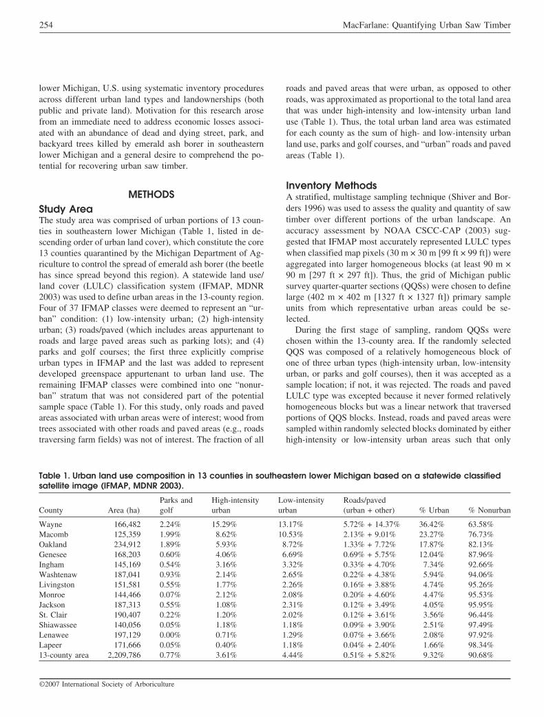
roads and paved areas that were urban, as opposed to otherroads, was approximated as proportional to the total land areathat was under high-intensity and low-intensity urban landuse (Table 1). Thus, the total urban land area was estimatedfor each county as the sum of high- and low-intensity urbanland use, parks and golf courses, and “urban” roads and pavedareas (Table 1).
Inventory MethodsA stratified, multistage sampling technique (Shiver and Bor-ders 1996) was used to assess the quality and quantity of sawtimber over different portions of the urban landscape. Anaccuracy assessment by NOAA CSCC-CAP (2003) sug-gested that IFMAP most accurately represented LULC typeswhen classified map pixels (30 m × 30 m [99 ft × 99 ft]) wereaggregated into larger homogeneous blocks (at least 90 m ×90 m [297 ft × 297 ft]). Thus, the grid of Michigan publicsurvey quarter-quarter sections (QQSs) were chosen to definelarge (402 m × 402 m [1327 ft × 1327 ft]) primary sampleunits from which representative urban areas could be se-lected.
During the first stage of sampling, random QQSs werechosen within the 13-county area. If the randomly selectedQQS was composed of a relatively homogeneous block ofone of three urban types (high-intensity urban, low-intensityurban, or parks and golf courses), then it was accepted as asample location; if not, it was rejected. The roads and pavedLULC type was excepted because it never formed relativelyhomogeneous blocks but was a linear network that traversedportions of QQS blocks. Instead, roads and paved areas weresampled within randomly selected blocks dominated by eitherhigh-intensity or low-intensity urban areas such that only
Table 1. Urban land use composition in 13 counties in southeastern lower Michigan based on a statewide classifiedsatellite image (IFMAP, MDNR 2003).
County Area (ha)Parks andgolf
High-intensityurban
Low-intensityurban
Roads/paved(urban + other) % Urban % Nonurban
Wayne 166,482 2.24% 15.29% 13.17% 5.72% + 14.37% 36.42% 63.58%Macomb 125,359 1.99% 8.62% 10.53% 2.13% + 9.01% 23.27% 76.73%Oakland 234,912 1.89% 5.93% 8.72% 1.33% + 7.72% 17.87% 82.13%Genesee 168,203 0.60% 4.06% 6.69% 0.69% + 5.75% 12.04% 87.96%Ingham 145,169 0.54% 3.16% 3.32% 0.33% + 4.70% 7.34% 92.66%Washtenaw 187,041 0.93% 2.14% 2.65% 0.22% + 4.38% 5.94% 94.06%Livingston 151,581 0.55% 1.77% 2.26% 0.16% + 3.88% 4.74% 95.26%Monroe 144,466 0.07% 2.12% 2.08% 0.20% + 4.60% 4.47% 95.53%Jackson 187,313 0.55% 1.08% 2.31% 0.12% + 3.49% 4.05% 95.95%St. Clair 190,407 0.22% 1.20% 2.02% 0.12% + 3.61% 3.56% 96.44%Shiawassee 140,056 0.05% 1.18% 1.18% 0.09% + 3.90% 2.51% 97.49%Lenawee 197,129 0.00% 0.71% 1.29% 0.07% + 3.66% 2.08% 97.92%Lapeer 171,666 0.05% 0.40% 1.18% 0.04% + 2.40% 1.66% 98.34%13-county area 2,209,786 0.77% 3.61% 4.44% 0.51% + 5.82% 9.32% 90.68%
254 MacFarlane: Quantifying Urban Saw Timber
©2007 International Society of Arboriculture
urban roads and paved areas would be sampled (as describedpreviously).
For the second stage of sampling, field crews visited eachselected QQS sample unit and systematically sampled a vari-able number of variable-area plots that combined to coverurban portions of the total QQS area. The field crew beganfrom an arbitrarily determined point along the edge of a QQS(generally determined by road access) and then moved acrossthe QQS systematically in a serpentine pattern. Permission tosample on private land was obtained in the field, or occasion-ally in advance; a portion of potential sample space was notsampled as a result of lack of landowner permission. Variablearea rectangular plots were systematically established usingone of the following three methods applied to the four dif-ferent IFMAP LULC classes:
1. If the area was either high- or low-intensity urban resi-dential or commercial, each ownership was considereda variable area plot. Lot dimensions (property bound-aries within the QQS) were approximated by a rectangleand all trees inside the rectangle were part of the po-tential sample population (including all buildings,paved and mowed areas within the property bound-aries).
2. Roads/paved areas were measured as variable area rect-angles bounded by the outer edge of sidewalks, curbs,or pavement; as such, they included pavement side-walks and mowed areas if they were between the side-walk and the curb or pavement. Trees that were grow-ing outside of this envelope (most typically trees thatwere planted between the sidewalk and a lawn or struc-ture) were not considered as road trees/paved areatrees (these trees ended up in one of the other urbanstratum).
3. If the area was a park or a golf course, then beginningfrom an arbitrary starting point along the edge of theQQS, the field crew defined a series of plot boundarylines that were approximately equidistant between twoareas of treed space (e.g., two rows of planted treesalong a fairway) creating variable area rectangularplots, which included intervening areas between groupsof trees or isolated trees (e.g., mowed grass).
The third stage of sampling involved selecting sample treesof all species within plots that met the common minimum sizestandard for saw timber trees in Michigan: 20 cm (8 in) orgreater stem diameter at breast height (1.37 m [4.5 ft]) dbh.Live, dying, standing dead trees were all measured; stumpswere measured at stump height (typically ≈10 to 20 cm [4 to8 in]) aboveground level. On each tree selected, the followingwas recorded for estimating saw timber quantity, quality, andaccessibility: species (if identifiable, e.g., on stumps and deadtrees), stem diameter (at breast or stump height as above), andtotal tree height and total saw timber log length in the main
stem to an approximately 20 cm (4 in) top diameter outsidebark (DOB) (measured with a Wheeler� pentaprism, ForestrySuppliers Inc., Jackson, MS), also known as “merchantable”height (Avery and Burkhart 1994). If the main stem forked,the largest of the forks was followed to assess merchantableheight; the other forks were considered part of the crown’sbranches.
The number of 2.4 m (8 ft) branch logs in a tree’s crownwith a minimum 20 cm (4 in) small end diameter DOB in thetree’s crown (8 ft [2.4 m] is the standard log length on Michi-gan timberlands) was also tallied on any tree with largeenough branches in its crown. In typical forest inventories,tree branches are not tallied and saw timber volume is esti-mated only for the main stem using information on merchant-able height, dbh, and some geometric model of a tree’s stem(e.g., a stem taper model; Zakrzewski and MacFarlane 2006).Urban (i.e., open)-grown trees have a much greater propor-tion of wood and larger branches in their crowns relative toforest-grown grown trees, however, so merchantable (senseAvery and Burkhart 1994) crown wood was tallied to accountfor this potential source of saw timber.
To assess wood quality, each tree was assigned a saw loggrade using six grading classes for hardwoods (Rast et al.1973): (0) no saw volume, (1) grade 1 saw timber, (2) grade2 saw timber, (3) grade 3 saw timber, (4) construction grade,and (5) local use class, which aligned with tree gradingclasses used by the U.S.D.A. Forest Service in the nationalforest inventory (Miles et al. 2001). Only four grading classeswere used for softwoods: (0) no saw volume, (1) grade 1 sawtimber, (2) grade 2 saw timber, and (3) grade 3 saw timber,consistent with common softwood grading rules (Avery andBurkhart 1994). Crown logs were not graded as a result oflack of an objective standard for doing so.
To assess the accessibility of merchantable wood in it, eachtree was classified into one of three accessibility classes rep-resenting the effort that would be involved in extracting thetimber from the tree:
1. Easily accessible � tree could be cut into relativelylong sections and could be felled with minimal risk ofproperty damage; cut sections could be loaded readilyonto a vehicle for transport.
2. Moderately accessible � tree could be cut into mer-chantable-length sections but would require additionaleffort to access with enhanced risk of property damage;cut sections would have to be transported a modestdistance to be loaded onto a vehicle for transport (atruck could not drive up near the tree).
3. Difficult to access � much of the tree would have to becut into submerchantable lengths to remove and/or treescould not be accessed without major effort (e.g., a largetree build into a deck) or a high likelihood of propertydamage.
Arboriculture & Urban Forestry 33(4): July 2007 255
©2007 International Society of Arboriculture

Data AnalysisTree Wood Volume EstimationStem measurements were used to estimate the total merchant-able saw timber round wood volume (m3) in each sample treefrom 0.15 cm (0.06 in) stump height to an approximate 20 cm(8 in) top DOB with Smalian’s formula (Avery and Burkhart1994). An individual taper model for each tree derived fromits top diameter and dbh was used to account for stem taperduring volume calculations (change in stem diameter over loglength was extrapolated to predict stump diameter outsidebark for each tree). A species-level constant bark factormodel, predicting wood volume inside bark from wood vol-ume outside bark, was used to estimate solid wood and barkvolumes from total volume (Smith 1985). Exotic tree specieswere assigned a bark factor of a species in the same generawith an equivalent bark type. Recovered sawn lumber volumein standing trees was computed using the tree’s taper modeland the International 1⁄4 in Board-foot rule for variable lengthlogs (Freese 1973) so that recovered saw lumber could becompared with cubic round wood volume estimates (i.e., ac-counting for losses attributable to sawing). Crown woodboard-foot volume was estimated using a model relating thebasal area (BAi, ft2) and the number of merchantable 8 ft(26.4 m) saw logs (Li) in the crown of a tree to its Interna-tional 1⁄4 in Board-foot rule volume (VSi): VSi � 19.30 (BAi
Li)0.74 derived from felled and dissected trees on Michigan
timberlands (MacFarlane, unpublished).
Scaling Up Individual Tree Estimates to the13-County RegionAverage saw timber volume per hectare (m3 and bd ft) wasestimated from the number of sample trees 20 cm (8 in) dbhor greater on a sample plot with an area ai. The contributionof each sample tree to per hectare estimates was weightedaccording to its selection probability, which was proportionalto the size of the variable area plot on which it occurred(Shiver and Borders 1996); the variance of sample means wasalso weighted in the same way. Estimates from each of theLULC classes were then combined to estimate the overallurban condition for the 13-county region using typical pro-cedures for combining stratum in stratified sampling (Shiverand Borders 1996) with contributions of plots from eachLULC weighted by the fraction of urban area they comprised(Table 1).
RESULTSOverall, 76 urban QQSs were surveyed and 1887 stems andstumps 20 cm (8 in) or greater were measured translating intoa mean density of 12.8 [±2.1 (standard error of mean) stemsand stumps ha−1 (5.8 [±0.8] ac−1) across the 13-county urbanarea; 89.7% were healthy, live trees, 6.3% were classed asdying, 3.7% were stumps, and 0.3% were dead, standing
trees. Estimated density values for LULCs were 9.5 [±3.1],13.7 [±3.5], 18.8 [±4.2], and 20.3 [±3.7] stems and stumpsha
−1
for high-intensity urban, low-intensity urban, parks andgolf courses, and roads and paved areas, respectively. At least68 species (with 20 cm [8 in] or greater) representing 36genera were found (some trees were only identified to theirgeneric scientific name and species could not be identified forall stumps); each was assigned to a species-product class (seeAppendix) based on U.S.D.A. Forest Inventory and Analysisgroupings (Miles et al. 2001).
Urban Wood Volume Grade and Species-ProductsThe mean urban (round) wood volume across the 13-countyarea in tree stem sections 20 cm (8 in) or greater dbh wasestimated to be 7.9 [±1.3] m3/ha−1 (117.2 ± 19.9 ft3/ac−1),≈31% of which was graded as having no saw timber value(grade 0; Table 2) as a result of major rot, defects, and otherproblems (see Rast et al. 1973). Approximately 56% of allgraded (not including crown wood) softwood volume per acrewas deemed as having no saw timber value, whereas only35% of potentially commercial hardwood stems were gradedas unfit for saw timber products (Table 2). Approximately73% of all stems of “noncommercial” species (Table 1) wererated as unsuited for saw timber. Less than 5% of red oak(shingle oak, Quercus imbricaria; pin oak, Q. palustris;northern red oak, Q. rubra; black oak, Q. velutina), white oak(white oak, Q. alba; swamp white oak, Q. bicolor; bur oak, Q.macrocarpa; English oak, Q. robur), and black walnut (Ju-glans nigra) wood was rated as having no value, whereas alarge proportion of hard maple (58%) (hedge maple, Acercampestre; black maple, A. nigrum; sugar maple, A. saccha-rum) and soft maple (42%) (boxelder, A. negundo; Norwaymaple, A. platanoides; red maple, A. rubrum; silver maple, A.saccharinum) wood was graded as having no saw timbervalue.
Approximately 60% of mean urban wood volume was sawtimber grade (grades 1 through 5; Table 2) amounting to 4.7m3/ha−1 [±0.9] (67.7 [±13.3] ft3/ac−1). Mean saw timber(round) wood volume translated into 1364 bd ft per urbanhectare (552 bd ft/ac−1) of sawn lumber using the Interna-tional 1⁄4 in rule (a conversion ratio of 290 bd ft per cubicmeter of wood [8.2 bd ft/ft3]). Most (93%) of urban softwoodsaw timber volume assigned to the lowest class (grade 3).This likely was the result of the greatly increased size anddensity of branch knots in open-grown coniferous trees,which are reflected in softwood grading rules (DeBell et al.1994; Uusitalo and Isotalo 2005). In general, a smaller pro-portion of urban hardwood saw timber volume was in highergrade classes than in lower grade classes (11% grade 1, 13%grade 2, 24% grade 3, and 48% grade 5) except for grade 4,construction grade, which comprised only 4%. The latter re-flects reservations by field technicians regarding the potential
256 MacFarlane: Quantifying Urban Saw Timber
©2007 International Society of Arboriculture

strength and durability of urban-grown saw timber trees (i.e.,these were conservatively placed in grade 5).
Approximately 89% of all urban saw timber volume (4.2m3/ha−1) was comprised of wood from commercially recog-nized hardwood species, 10% from commercial softwoodspecies (0.5 m3/ha−1), and the remaining 1% from noncom-mercial species (Table 2). Approximately one-fourth of allcommercial hardwood saw timber was comprised of softmaple alone, and nearly two-thirds was comprised of softmaple, poplar (bigtooth aspen, Populus grandidentata; quak-ing aspen, P. tremuloides; cottonwood, P. deltoides), ash(white ash, Fraxinus americana; European ash, F. excelsior;green ash, F. pennsylvanica), and red oak (Table 2). Blackwalnut, red oak, and poplar trees had more than double theaverage proportion of high-grade wood (grades 1 through 3)in them, whereas the majority of saw timber from soft maplesand other hard and other soft hardwood species (mostly hon-eylocust [Gleditsia triacanthos] and elm [Ulmus americana,U. pumila], respectively) was rated in the lowest lumbergrade classes (4 and 5; Table 2). More than three-fourths ofall softwood saw timber was comprised of low-grade spruce-fir (Colorado blue spruce, Picea pungens; Norway spruce,
P. abies; white spruce, P. glauca; white fir, Abies concolor)and white (Pinus strobus) and red pines (P. resinosa).
Across all species product-classes, ≈9% of mean urbanwood volume (Table 2) was composed of crown logs of vari-able (unknown) quality amounting to 0.7 [±0.2] m3/ha−1
(10.2 [±2.4] ft3/ac−1] of saw timber volume. The 0.7 m3/ha−1
of crown wood translated into 176 bd ft/ha−1 (72 bd ft/ac−1)of ungraded urban saw timber. Over half of this (0.4 m3/ha−1)was found in the crowns of soft (mostly silver) maple trees.Honeylocust, cottonwood, elm, and white oak trees also hadsignificant amounts of saw-grade branch wood. Noncommer-cial species (mostly willow [Salix spp.] and ornamental apple[Malus spp.] and cherry [Prunus spp.] trees) had a significantproportion of their potential sawn timber in their crowns, butthe absolute amounts were trivial. Urban softwoods also hadinsignificant amounts of saw-grade branch wood (Table 2),which was not surprising given their naturally excurrentgrowth form.
Regional Urban Saw Timber AbundanceThe overall weighted mean urban saw timber volume forstem and crown wood in the 13-county area was estimated to
Table 2. Mean volume (m3/ha−1) of tree stem and branch sections 20 cm (8 in) or greater in diameter in urban areasof SE lower Michigan by species-product class and wood products grade.z
Spp-product class
Main stem grade
CrownTotalvolume
Total grade(1–5)
% Crownwood0 1 2 3 4 5
SoftwoodsSpruce-fir 0.3177 — 0.0021 0.2831 — — — 0.6029 0.2852 0.00%White-red pine 0.1619 — 0.0035 0.1128 — — 0.0032 0.2812 0.1162 1.13%Other pine 0.1218 0.0079 0.0193 0.0173 — — 0.0012 0.1675 0.0445 0.74%Other softwoods 0.0046 — — 0.0389 — — 0.0002 0.0437 0.0389 0.44%Douglas-fir 0.0025 — — 0.0040 — — — 0.0065 0.0040 0.00%All softwoods 0.6084 0.0079 0.0249 0.4560 — — 0.0046 1.1018 0.4887 0.42%HardwoodsSoft maple 1.0385 0.0032 0.0737 0.0918 0.0069 0.8172 0.4131 2.4444 0.9928 16.90%Poplar 0.0951 0.2366 0.1398 0.2550 0.0034 0.0390 0.0586 0.8275 0.6738 7.08%Red oak 0.0070 0.0309 0.1040 0.2458 0.0210 0.2405 — 0.6494 0.6423 0.00%Ash 0.0718 0.0924 0.0853 0.0203 0.0164 0.2527 0.0162 0.5550 0.4670 2.92%Other soft hardwoods 0.1844 0.0179 — 0.1010 0.0229 0.2421 0.0505 0.6188 0.3839 8.16%White oak 0.0130 0.0181 0.0130 0.1157 0.0352 0.1037 0.0596 0.3583 0.2856 16.65%Hickory 0.0555 — 0.0017 0.0956 0.0371 0.0308 0.0152 0.2359 0.1652 6.44%Walnut 0.0016 0.0248 0.0747 0.0254 — 0.0329 0.0037 0.1632 0.1578 2.26%Other hard hardwoods 0.0810 0.0050 0.0088 0.0333 0.0101 0.0928 0.0424 0.2735 0.1501 15.52%Hard maple 0.2082 0.0013 0.0175 0.0376 0.0184 0.0622 0.0142 0.3594 0.1370 3.96%Basswood 0.0399 0.0142 0.0197 0.0019 — 0.0657 0.0209 0.1624 0.1016 12.88%Birch 0.0064 — — — — 0.0622 0.0024 0.0710 0.0622 3.34%Yellow poplar — — — 0.0001 — — — 0.0001 0.0001 0.00%All hardwoods 1.8025 0.4444 0.5383 1.0235 0.1715 2.0418 0.6969 6.7189 4.2195 10.37%Noncommercial 0.0633 — 0.0089 0.0056 — 0.0094 0.0116 0.0989 0.0239 11.75%All spp-product classes 2.4742 0.4523 0.5721 1.4851 0.1715 2.0512 0.7131 7.9196 4.7322 9.00%zCrown logs were not graded.Dashes indicate no trees of this type were found during sampling.
Arboriculture & Urban Forestry 33(4): July 2007 257
©2007 International Society of Arboriculture

be 5.4 [±1.7] m3/ha−1, or 1540 [±485] bd ft/ha−1 accountingfor conversion of round wood to dimensional lumber. Therewas considerable variation in saw timber volume both be-tween and within different urban LULCs. Mean graded sawtimber volume was 3.0 [±1.2], 5.3 [±1.6], 7.8 [±2.1], and 7.4[±1.7] m3/ha−1, respectively, for high-intensity urban, low-intensity urban, parks and golf courses, and roads and pavedareas. Estimated crown wood saw timber volume for high-intensity urban, low-intensity urban, parks and golf courses,and roads and paved areas was 0.4 [±0.2], 0.7 [±0.3], 1.0[±0.3], and 2.1 [±0.6] m3/ha−1, respectively. Scaled up to the13-county region, this amounts to a total standing volume of1.15 million m3 of urban saw timber (≈327 million bd ft ofdimensional lumber) (Table 3).
AccessibilityTo successfully recover saw timber from a tree, the tree mustbe accessible, i.e., able to be felled, cut in sections of mer-chantable length, and delivered to a sawmill (in urban areas,portable sawmills can ease the latter burden). Accessibilitywas not equal across all urban land types (Obviously, itshould be much easier to harvest wood from street andparkland trees than from around homes and offices.). Ap-proximately 93.5% of all saw timber on parks and golfcourses was considered easily accessible and less than 1%difficult to access. Almost 90% of saw timber along roadsand paved areas was rated as easily accessible, although streettrees were approximately four times (2.1% versus 0.5%)more likely to be rated as difficult to access than trees onparks and golf courses with the main complication beingextracting wood from occasional large trees whose crownsare closely intertwined with utility wires. High-intensity ur-ban areas posed a greater challenge for extracting saw timberfrom trees, although less than 4% of this saw timber wasconsidered difficult to access. By sharp contrast, approxi-
mately half of all saw timber in low-intensity urban areas wasrated as difficult to access. This reflects the close proximityof many large trees to hazards (sense Matheny and Clark1994) such as homes or fences, in low-intensity urban areas,that would necessitate extraordinary measures to harvest treesin standard log lengths. Based on the weighted contributionof each of the four urban LULCs to total urban area (Table 1),it was estimated that ≈56% of all urban saw timber in the13-county area was easily accessible, another 16% wouldrequire some additional measures to extract that would addadditional costs (moderately accessible), and the remaining28% difficult (for most intents and purposes considered in-accessible). Thus, of the total standing urban saw timber,≈72% was considered accessible for extraction, amounting to825,000 m3 of urban saw timber (≈235 million bd ft of di-mensional lumber) (Table 3).
Annual YieldThe 825,000 m3 of urban saw timber that is accessible in the13-county areas includes all standing trees, virtually all ofwhich would not be harvested until the trees that contain themwere dead, or at minimum dying. Thus, to calculate the avail-ability of urban saw timber on an annual basis, it was nec-essary to estimate the rate at which trees would become avail-able. However, mortality rates and removal rates could not bedirectly assessed from the data collected for this study(stumps, e.g., represent death events from different years andmay be ground up and seeded over and thus might not betallied at all). Instead, recent estimates by Nowak et al. (2004)describing general trends and specific tree removal and mor-tality rates were combined with the data presented here andused to make reasonable estimates of urban saw timber avail-ability on an annual basis.
Nowak et al. (2004) suggested that standing trees in ap-parently good condition die at a rate of ≈1.4% per year. The
Table 3. Saw timber volume estimates (m3) for urban portions of 13 counties in southeastern lower Michigan.
County Total standing Accessible Annual yield
Genesee 109,358 (34,428) 78,738 (24,788) 1575 (496)Ingham 57,5 (18,124) 41,450 (13,049) 829 (261)Jackson 41,013 (12,912) 29,529 (9296) 591 (186)Lapeer 15,426 (4856) 11,107 (3497) 222 (70)Lenawee 22,094 (6956) 15,908 (5008) 318 (100)Livingston 38,813 (12,219) 27,945 (8798) 559 (176)Macomb 157,526 (49,591) 113,419 (35,706) 2,268 (714)Monroe 34,835 (10,967) 25,081 (7896) 502 (158)Oakland 226,736 (71,380) 163,250 (51,394) 3,265 (1028)Shiawassee 18,971 (5972) 13,659 (4300) 273 (86)St. Clair 36,594 (11,520) 26,348 (8295) 527 (166)Washtenaw 60,017 (18,894) 43,212 (13,604) 864 (272)Wayne 327,415 (103,075) 235,739 (74,214) 4,715 (1484)13-county area 1,146,368 (360,894) 825,385 (259,844) 16,508 (5,197)
Standard errors in parentheses.
258 MacFarlane: Quantifying Urban Saw Timber
©2007 International Society of Arboriculture

latter rate was used to describe mortality in the “live” cat-egory in this study, 1.4% of the 89.7% of urban stems peracre or 1.3%. Trees with crown deterioration, equatingroughly to “dying” trees in this study, had a mortality rate of≈6.4% (Nowak et al. 2004), which equates to 0.4% more ofthe trees in this study. Ignoring the stumps, another 0.3% canbe tallied from dead standing trees that have not yet beenremoved. All totaled, it can be expected that ≈2% of theaccessible volume would come available annually, whichtranslates into ≈16,500 m3 (or ≈4.7 million bd ft) of urbansaw timber per year available in the 13-county study area(Table 3).
DISCUSSIONThe methods presented here allowed for a regional estimateof urban saw timber to be developed and extrapolated throughurban land area estimates derived from satellite photography.Data describing urban land cover are generally widely avail-able (e.g., the entire United States; Nowak et al. 2006); thus,these methods could be replicated almost anywhere. To theextent that average per hectare estimates derived from urbanareas in southeastern lower Michigan are representative ofbroader regional species composition and urban tree demo-graphic structure, these specific estimates could be furtherextrapolated outside of this specific region. However, theoverall weighted estimates are also sensitive to the relativemakeup of urban areas (e.g., a different ratio of high- versuslow-intensity urban areas) such that per hectare estimates forurban LULCs would need to be reweighted accordingly.
Over 16,000 m3 of urban saw timber is estimated to comeavailable each year in the 13-county study area. To put thisnumber in perspective, small modern sawmills process ≈3000to 10,000 m3 of wood per year annually (Pascal Kamdem,Michigan State University, pers. com.). Assuming a mini-mum of 3000 m3 to remain viable, all of the potentiallyavailable wood in the 13 counties that comprise southeasternlower Michigan could support the minimum annual needs offive of these mills. The 4.7 million bd ft of lumber annuallyavailable in urban trees in this region is equivalent to theamount of wood used to build 362 average-sized homes (Falk2002).
The quality of wood in urban softwoods was generally lowbased on the grading standards applied, which was not sur-prising given the importance of maintaining small branchknots along the main stem of (coniferous) trees to softwoodquality; a condition most likely to be met when trees areforest grown (DeBell et al. 1994; Uusitalo and Isotalo 2005).However, most urban saw timber (≈90%) inventoried camefrom commercially viable hardwood timber species, 60% ofwhich was considered saw-grade quality. Whereas noncom-mercial species comprise a trivial proportion of large trees,wood from exotic species did comprise a substantial propor-tion of urban wood (e.g., Siberian elm, Norway maple, and
horsechestnut), raising potential concerns regarding their uti-lization (e.g., commercial kiln-drying procedures have notbeen developed for them). However, wood from many ofthese species are already commercially viable (Norway mapleis considered a valuable hardwood in Germany; Jurek andWihs 1998), and some North American vendors have beenable sell wood from exotic tree species at a premium (www.urbantreesalvage.com).
One aspect of urban wood quality not addressed by thisstudy is that of the mechanical properties of urban wood.Mackes et al. (2005) found that the modulus of rupture andmodulus of elasticity were both lower in open-grown trees,primarily attributable to a greater quantity of juvenile wood,which suggests a potentially lower strength for “urban”wood. Further research would have to be done to specificallymeasure wood properties of urban versus forest-grown trees.
The estimates of urban saw timber presented here are likelyconservative based on the definitions of “urban” area used inthis study. The use of remotely sensed land use/land coverimagery to define urban areas likely underestimates the num-ber of trees in urban areas relative to definitions based onpolitical boundaries such as city limits or census districts(e.g., Nowak et al. 2006), which, if used, would have in-cluded wood from trees growing in forested areas withinurban zones. It also likely underestimates the total amount ofurban area. In a recent study, Fang et al. (2006) demonstratedthat land use maps were more likely to misclassify urbanareas (in Chicago) as forested than the reverse, because of thefact that many houses were beneath a canopy of trees.
Estimates of urban saw timber availability were also likelyconservative based on definitions of what portion of urbanwood qualified as extractable sawn wood products. Low-intensity urban areas comprised almost half of all urban areain the 13-county region (Table 1) and almost 50% of thewood in these areas was rated as difficult to access attribut-able to a frequent close proximity of large trees to potentialhazards (e.g., homes). Sherrill (2003) proposed reasonableguidelines for safely extracting urban wood and commercialarborists to safely remove such trees all the time; thus, alarger proportion of wood from these trees may actually beaccessible. Advances in sawing technology might also allowportions of some of the wood rated as grade 0 to be used forsaw timber. Typical modern sawmills often dissect logs intoa variety of component parts of different grades such that thevisually based whole log or tree stem grading rules used here(e.g., Rast et al. 1973) may be overly conservative.
Estimates also did not include the solid wood productspotential of trees smaller than 20 cm (8 in) diameter. Ad-vances in wood technology have greatly expanded the poten-tial for smaller trees (LeVan-Green and Livingston 2001).However, by extrapolating volume estimates for trees of dif-ferent sizes measured in this study, it was estimated that treesless than 20 cm (8 in) contribute only ≈3% to the total un-
Arboriculture & Urban Forestry 33(4): July 2007 259
©2007 International Society of Arboriculture
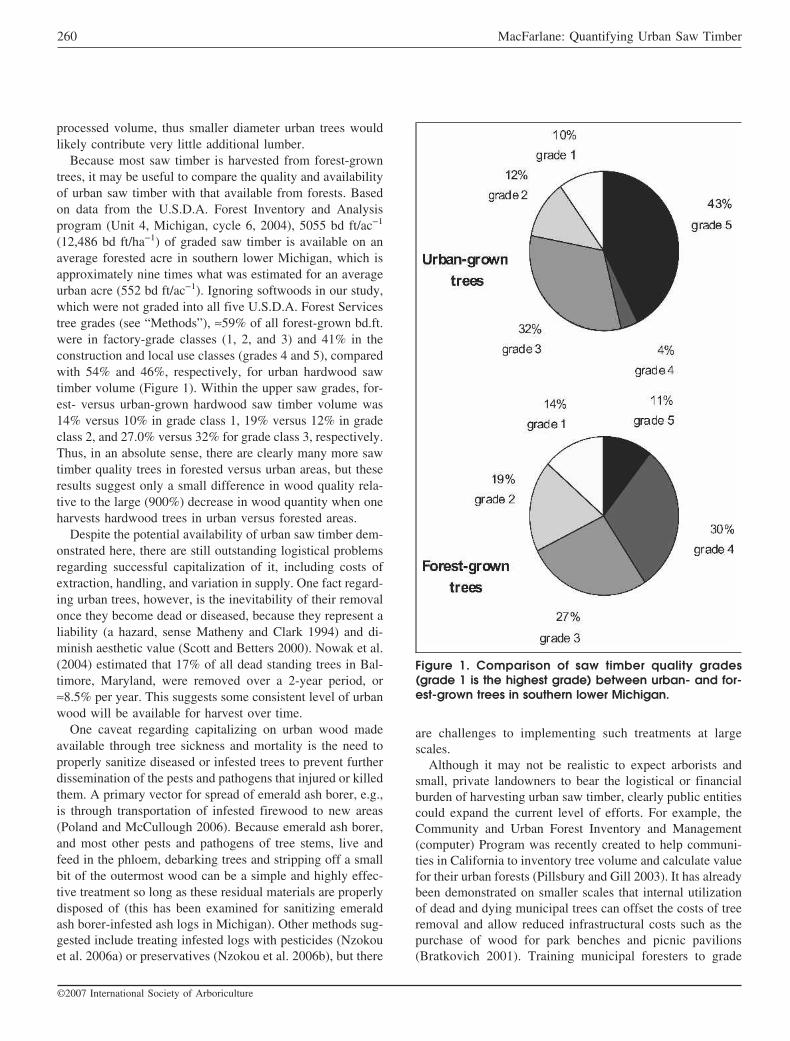
processed volume, thus smaller diameter urban trees wouldlikely contribute very little additional lumber.
Because most saw timber is harvested from forest-growntrees, it may be useful to compare the quality and availabilityof urban saw timber with that available from forests. Basedon data from the U.S.D.A. Forest Inventory and Analysisprogram (Unit 4, Michigan, cycle 6, 2004), 5055 bd ft/ac−1
(12,486 bd ft/ha−1) of graded saw timber is available on anaverage forested acre in southern lower Michigan, which isapproximately nine times what was estimated for an averageurban acre (552 bd ft/ac−1). Ignoring softwoods in our study,which were not graded into all five U.S.D.A. Forest Servicestree grades (see “Methods”), ≈59% of all forest-grown bd.ft.were in factory-grade classes (1, 2, and 3) and 41% in theconstruction and local use classes (grades 4 and 5), comparedwith 54% and 46%, respectively, for urban hardwood sawtimber volume (Figure 1). Within the upper saw grades, for-est- versus urban-grown hardwood saw timber volume was14% versus 10% in grade class 1, 19% versus 12% in gradeclass 2, and 27.0% versus 32% for grade class 3, respectively.Thus, in an absolute sense, there are clearly many more sawtimber quality trees in forested versus urban areas, but theseresults suggest only a small difference in wood quality rela-tive to the large (900%) decrease in wood quantity when oneharvests hardwood trees in urban versus forested areas.
Despite the potential availability of urban saw timber dem-onstrated here, there are still outstanding logistical problemsregarding successful capitalization of it, including costs ofextraction, handling, and variation in supply. One fact regard-ing urban trees, however, is the inevitability of their removalonce they become dead or diseased, because they represent aliability (a hazard, sense Matheny and Clark 1994) and di-minish aesthetic value (Scott and Betters 2000). Nowak et al.(2004) estimated that 17% of all dead standing trees in Bal-timore, Maryland, were removed over a 2-year period, or≈8.5% per year. This suggests some consistent level of urbanwood will be available for harvest over time.
One caveat regarding capitalizing on urban wood madeavailable through tree sickness and mortality is the need toproperly sanitize diseased or infested trees to prevent furtherdissemination of the pests and pathogens that injured or killedthem. A primary vector for spread of emerald ash borer, e.g.,is through transportation of infested firewood to new areas(Poland and McCullough 2006). Because emerald ash borer,and most other pests and pathogens of tree stems, live andfeed in the phloem, debarking trees and stripping off a smallbit of the outermost wood can be a simple and highly effec-tive treatment so long as these residual materials are properlydisposed of (this has been examined for sanitizing emeraldash borer-infested ash logs in Michigan). Other methods sug-gested include treating infested logs with pesticides (Nzokouet al. 2006a) or preservatives (Nzokou et al. 2006b), but there
are challenges to implementing such treatments at largescales.
Although it may not be realistic to expect arborists andsmall, private landowners to bear the logistical or financialburden of harvesting urban saw timber, clearly public entitiescould expand the current level of efforts. For example, theCommunity and Urban Forest Inventory and Management(computer) Program was recently created to help communi-ties in California to inventory tree volume and calculate valuefor their urban forests (Pillsbury and Gill 2003). It has alreadybeen demonstrated on smaller scales that internal utilizationof dead and dying municipal trees can offset the costs of treeremoval and allow reduced infrastructural costs such as thepurchase of wood for park benches and picnic pavilions(Bratkovich 2001). Training municipal foresters to grade
Figure 1. Comparison of saw timber quality grades(grade 1 is the highest grade) between urban- and for-est-grown trees in southern lower Michigan.
260 MacFarlane: Quantifying Urban Saw Timber
©2007 International Society of Arboriculture
trees would be an important first step toward differentiatingthe value of dead and dying trees. The alternative is to con-tinue to put valuable wood products contained in urban treesto some lesser use (e.g., firewood) or, as a worst case, into alandfill (urban wood waste comprises ≈17% of all waste re-ceived at U.S. landfills; Solid Waste Association of NorthAmerica 2002).
CONCLUSIONRecent economic losses associated with the destruction ofurban trees by wood-boring forest pests such as the emeraldash borer highlights the well-known value associated withurban forests, not the least of which may be the valuablewood in the trees. Although there are potential concerns withharvesting urban trees for saw timber such as low availabilityand poor wood quality, the results of this study suggest thatmany of them may be unfounded. Harvesting urban wood iscertainly less efficient relative to commercial logging in for-ests because, even if abundant, urban wood may be scatteredaround a large metropolitan area in smaller saleable units,greatly increasing the cost of consolidating and transportingit. However, it may not be prudent to view urban wood as analternative to wood derived from forests. Rather, it might bestbe viewed as a supplementary source of wood that may helpto offset the social and economic costs of urban tree removaland urban wood waste disposal to private landowners andgovernment entities. Clearly, if southeastern lower Michiganis similar to other regions nationwide, a substantial amount ofwood products volume is available from trees in urban areas.
Acknowledgments. I thank the Southeast Michigan Resource Con-servation and Development Council and the Michigan AgriculturalExperiment Station for providing funding and resources for thisresearch. I also thank Sam Sherrill and Pascal Kamdem for thought-ful comments regarding this research. I thank John Kemppainen,Sean Flinn, and Hong Su An for spending many hours knocking ondoors and measuring urban trees.
LITERATURE CITEDAvery, T.E., and H.E. Burkhart. 1994. Forest Measurements.
4th edition. McGraw-Hill, Inc., New York.Bratkovich, S.M. 2001. Utilizing Municipal Trees: Ideas
from Across the Country. NA-TP-06-01, St. Paul, MN:USDA, Forest Service, Northeastern Area, State and Pri-vate Forestry.
DeBell, J.D., J.C. Tappenier, and R.L. Kramer. 1994. Brachdiameter of western hemlock: Effects of precommercialthinning and implications for log grades. Western Journalof Applied Forestry 9:88–90.
Falk, B. 2002. Wood-framed building deconstruction: Asource of lumber for construction? Forest Products Jour-nal 52:8–15.
Fang, S., G. Gertner, G. Wang, and A. Anderson. 2006. Theimpact of misclassification in land use maps in the pre-
diction of landscape dynamics. Landscape Ecology 21:233–242.
Freese, F. 1973. A Collection of Log Rules. Gen. Tech. Rep.FPL-01. Madison, WI: U.S. Department of Agriculture,Forest Service, Forest Products Laboratory. U.S. Govern-ment Printing Office, 754-546/28.
Johnson, A.D., and H.D. Gerhold. 2001. Carbon storage byutility-compatible trees. Journal of Arboriculture 27:57–68.
Jurek, J., and U. Wihs. 1998. Norway maple in the city forestof Northeim. Site requirements and growth. Forst-und-Holz 53:15–18.
LeVan-Green, S.L., and J. Livingston. 2001. Exploring theuse for small-diameter trees. Forest Products Journal 51:10–21.
Mackes, K., W. Sheppard, and C. Jennings. 2005. Evaluatingthe bending properties of clear wood specimens producedfrom small-diameter ponderosa pine trees. Forest Prod-ucts Journal 55:72–80.
Matheny, N.P., and J.R. Clark. 1994. A Photographic Guideto the Evaluation of Hazard Trees in Urban Areas. 2ndedition. International Society of Arboriculture, Urbana, IL.
McPherson, E.G., J.R. Simpson, P.J. Peper, and Q. Xiao.1999. Benefit-cost analysis of Modesto’s municipal urbanforest. Journal of Arboriculture 25:235–248.
Michigan Department of Natural Resources (MDNR). ForestMineral and Fire Management Division. 2003. IFMAP/GAP Lower Peninsula Land Cover. Michigan Departmentof Natural Resources, Ann Arbor, MI. www.dnr.dtate.mi.us/spatialdatalibrary/sdl2/land_use_cover/2001/IFMAP_lp_landcover.htm (accessed 9/20/04).
Miles, P.D., G.J. Brand, C.L. Alerich, L.F. Bednar, S.W.Woudenberg, J.F. Glover, and E.N. Ezzell. 2001. The ForestInventory and Analysis Database: Database Descriptionand Users Manual, Version 1. GTR NC-218, U.S.D.A.Forest Service, North Central Forest Experiment Station.
NOAA CSCC-CAP. 2003. Late-date Classification of theLower Peninsula of Michigan. National Oceanic and At-mospheric Administration (NOAA) Coastal ServicesCenter (CSC)/Coastal Change Analysis Products(C-CAP), Charleston, SC.
Nowak, D.J., and D.E. Crane. 2002. Carbon storage and se-questration by urban trees in the USA. EnvironmentalPollution 166:381–389.
Nowak, D.J., M. Kuroda, and D.E. Crane. 2004. Tree mor-tality rates and tree population projections in Baltimore,Maryland, USA. Urban Forestry and Urban Greening 2:139–147.
Nowak, D.J., J.E. Pasek, R.A. Sequeira, D.E. Crane, and V.C.Mastro. 2001. Potential Effect of Anoplophora glabripen-nis (Coleoptera: Cerambycidae) on urban trees in theUnited States. Journal of Economic Entomology 94:116–122.
Arboriculture & Urban Forestry 33(4): July 2007 261
©2007 International Society of Arboriculture

Nowak, D.J., J.T. Walton, J.F. Dwyer, L.G. Kaya, and S.Meyong. 2006. The increasing influence of urban envi-ronments on U.S. forest management. Journal of Forestry103:377–382.
Nzokou, P., S.M. Pankras, and D.P. Kamdem. 2006a. Preser-vative treatment of ash wood from emerald ash borer(Agrilus planipennis) infested trees. Forest Products Jour-nal 56:69–72.
Nzokou, P., T.R. Petrice, R.A. Haack, and D.P. Kamdem.2006b. Borate and imidacloprid treatment of ash logs in-fested with the emerald ash borer. Forest Products Journal56:78–81.
Pillsbury, N.H., and S.J. Gill. 2003. A User Guide forCUFIM, the Community and Urban Forest Inventory andManagement Program. Tech. Report No. 11, Urban ForestEcosystems Institute, California Polytechnic State Uni-versity, San Luis Obispo, CA.
Poland, T.M., and D.G. McCullough. 2006. Emerald ashborer: Invasion of the urban forest and the threat to NorthAmerica’s ash resource. Journal of Forestry 104:118–124.
Rast, E.D., D.L. Sonderman, and G.L. Gammon. 1973. AGuide to Hardwood Log Grading. GTR-NE-1, U.S.D.A.Forest Service, Northeastern Forest Experiment Station.
Scott, J.L., and D.R. Betters. 2000. Economic analysis ofurban tree replacement decisions. Journal of Arboriculture26:69–77.
Sherrill, S.B. 2003. Harvesting Urban Timber: A Guide toMaking Better Use of Urban Trees. Linden PublishingInc., Fresno, CA.
Shiver, B.D., and B.E. Borders. 1996. Sampling Techniquesfor Forest Resource Inventory. John Wiley and Sons, Inc.,New York.
Smith, W.B. 1985. Factors and Equations to Estimate ForestBiomass in the North Central Region. U.S.D.A. ForestService, North Central Forest Experiment Station, Re-search Paper NC-268.
Solid Waste Association of North America. 2002. SuccessfulApproaches to Recycling Urban Wood Wastes. Gen.Tech. Rep. FPL-GTR-133. U.S.D.A., Forest Service, For-est Products Laboratory, Madison, WI.
Uusitalo, J., and J. Isotalo. 2005. Predicting knottiness ofPinus sylvestris for use in tree bucking procedures. Scan-dinavian Journal of Forest Research 20:521–533.
Zakrzewski, W.T., and D.W. MacFarlane. 2006. Regionalstem profile model for cross-border comparisons of har-vested red pine (Pinus resinosa Ait.) in Ontario andMichigan. Forest Science 52:468–475.
David W. MacFarlaneDepartment of Forestry Michigan State University126 Natural Resource BuildingEast Lansing, MI 48824, [email protected]
Résumé. Il y a besoin croissant dans la société pour employer desressources efficacement, et ce incluant l’utilisation des arbres mortsou mourants en milieux urbains. La récolte des billes de sciage àpartir des arbres urbains constitue une utilisation ultime, mais laplupart du temps le bois se retrouve enfoui, déchiqueté en copeauxde bois ou encore est employé comme biomasse pour la productiond’énergie. Pour évaluer la faisabilité générale de récolter le bois enmilieu urbain, une estimation régionale de la quantité de bois desciage, de sa qualité et de disponibilité a été faite auprès de 13comtés dans le Sud-Est du Bas Michigan. De manière conservatrice,un volume de plus de 16000 m3 de bois de sciage a été estimécomme étant disponible annuellement à partir des arbres morts oumourants au sein de cette étude, ce qui s’avérait suffisant pourassurer l’approvisionnement annuel minimum de cinq petites scier-ies. La qualité du bois mou en milieu urbain s’avérait plutôt faible,mais ce elle ne comptait que pour 10% du volume total récoltable enmilieu urbain. La qualité des bois durs en milieu urbain s’avéraitquant à elle comparable à celle retrouvée dans les forêts de la région,et ce même si les volumes absolus disponibles étaient de neuf foisinférieur. Même s’il existe des inquiétudes potentielles à propos dela récolte d’arbres en milieu urbain pour des fins de sciage, telles quela faible disponibilité et la faible qualité du bois, les résultats de cetteétude suggèrent que plusieurs d’entre elles pourraient s’avérer in-fondées.
Zusammenfassung. Es gibt eine wachsende Nachfrage nach ef-fektiver Resourcennutzung, inklusive einer effektiven Nutzung vontoten und sterbenden Bäumen in urbanen Gebieten. Die Holzerntevon Stadtbäumen ist eine hochwertige Nutzung, aber viel Holz ausurbanen Regionen endet in Landverfüllungen oder wird für Hacks-chnitzel oder Biotreibstoff verwendet. Um die generellen Möglich-keiten von der urbanen Holzernte zu bewerten, wurde für eine Ge-gend mit 13 Kommunen in Lower Michigan eine regionale Schät-zung der urbanen Holzquantität, -qualität und Verfügbarkeitvorgenommen. Konservativ werden jährlich über 16 Tausend m3 indieser Region an Totholz und absterbenden Bäumen geerntet,genug, um den jährlichen Minimalbedarf von 15 Sägemühlen zudecken. Die Holzqualität von urbanen Weichhölzern ist allgemeinniedrig, aber ihr Anteil beträgt auch nur 10 % an der Gesamternte.Die Holzqualität von urban geernteten Harthölzern ist vergleichbarmit den im Wald der Region geernteten Harthölzern, obwohl dasabsolute Volumen nur den neunten Teil betrug. Während es mögli-cherweise Bedenken zur urbanen Holzernte gibt, wie geringe Ver-fügbarkeit oder schlechte Qualität, zeigt doch diese Studie, dassviele Bedenken unbegründet sind.
Resumen. Existe una creciente necesidad social por utilizar efi-cientemente los recursos, incluyendo el uso efectivo de árbolesmuertos y moribundos en áreas urbanas. La cosecha de madera paraaserrío de los árboles urbanos está en uso, pero actualmente muchade ella termina en rellenos o es usada para astillas o biomasa com-bustible. Con el propósito de evaluar la factibilidad de cosecharmadera para aserrío se desarrolló una estimación regional de lacantidad, calidad y disponibilidad de madera urbana para un área delcondado en el sureste del Bajo Michigan. Conservadoramente, seestima que 16 mil m3 de madera están disponibles cada año en elárea de estudio de árboles muertos y moribundos, suficiente parasatisfacer las necesidades mínimas anuales de 5 aserraderos pe-queños. La cantidad de madera en los bosques de madera blanda fue
262 MacFarlane: Quantifying Urban Saw Timber
©2007 International Society of Arboriculture

generalmente baja, pero comprendió solamente una pequeña porción(10%) de la madera urbana. La calidad de la madera de los bosquesde madera dura fue comparable a la que se encuentra en los bosquesnativos en la región, a pesar de que el volumen absoluto fue nueveveces menor. Con todo y que hay preocupación sobre la cosecha delos árboles urbanos para madera aserrada, tales como baja dispon-ibilidad y pobre calidad de la madera, los resultados de este estudiosugieren que mucho de este temor es infundado.
Appendix. Study species and FIA species-product classassignments.
FIAspecies-productgroup Common name Latin name
Ash Ash, European Fraxinus excelsiorAsh, green Fraxinus pennsylvanicaAsh, white Fraxinus Americana
Basswood Basswood, American Tilia americanaLinden, littleleaf Tilia cordata
Birch Birch, river Betula nigraBirch, paper Betula papyrifera
Douglas-fir Douglas-fir Pseudotsuga menziesiiHard maple Maple, black Acer nigrum
Maple, hedge Acer campestreMaple, sugar Acer saccharum
Hickory Hickory, bitternut Carya cordiformisHickory, pignut Carya glabraHickory, shagbark Carya ovataHickory, shellbark Carya laciniosa
Noncommercial Apple Malus spp.Ornamental cherry/plum Prunus spp.Gingko Ginkgo bilobaHawthorn Crataegus spp.Mountainash, American Sorbus americanaPear, callery Pyrus calleryanaOlive-tree, Russian Elaeagnus angustifoliaTree-of-heaven Ailanthus altissimaWillow Salix spp.Willow, black Salix nigra
Other hardhardwoods Chestnut Castanea spp.
Honeylocust Gleditsia triacanthosLocust, black Robinia pseudoacacia
Appendix. Study species and FIA species-product classassignments. (continued)
FIAspecies-productgroup Common name Latin name
Other pine Pine, Austrian Pinus nigraPine, Scotch Pinus sylvestris
Other softwoods Baldcypress Taxodium distichumRedcedar, eastern Juniperus virginianaWhite-cedar, northern Thuja occidentalis
Other softhardwoods Buckeye Aesculus spp.
Catalpa, northern Catalapa speciosaCherry, black Prunus serotinaElm, American Ulmus americanaElm, Siberian Ulmus pumilaHackberry Celtis occidentalisHorsechestnut Aesculus hippocastanumPlanetree, London Platanus acerifoliaMulberry, red Morus rubraSassafras Sassafras albidumSweetgum Liquidambar styracifluaSycamore Platanus occidentalis
Poplar Aspen, bigtooth Populus grandidentataAspen, quaking Populus tremuloidesCottonwood, eastern Populus deltoides
Red oak Oak, black Quercus velutinaOak, northern red Quercus rubraOak, pin Quercus palustrisOak, shingle Quercus imbricaria
Soft maple Boxelder Acer negundoMaple, Norway Acer platanoidesMaple, red Acer rubrumMaple, silver Acer saccharinum
Spruce-fir Fir, white Abies concolorSpruce, Colorado blue Picea pungensSpruce, Norway Picea abiesSpruce, white Picea glauca
Walnut Walnut, black Juglans nigraWhite oak Oak, bur Quercus macrocarpa
Oak, English Quercus roburOak, swamp white Quercus bicolorOak, white Quercus alba
White-red pine Pine, eastern white Pinus strobusPine, red Pinus resinosa
Yellow poplar Yellow-poplar Liriodendron tulipifera
Arboriculture & Urban Forestry 33(4): July 2007 263
©2007 International Society of Arboriculture

L. renewaFuel Wood Dust MSDS
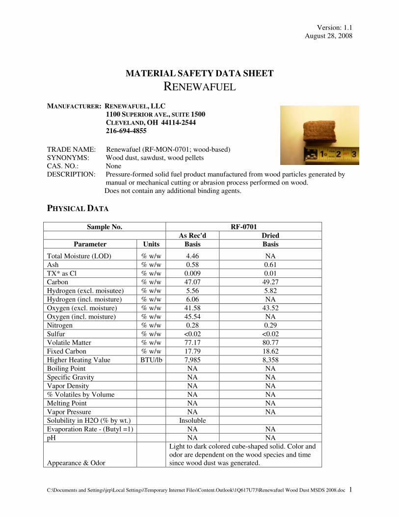
Version: 1.1
August 28, 2008
C:\Documents and Settings\jrp\Local Settings\Temporary Internet Files\Content.Outlook\1Q617U73\Renewafuel Wood Dust MSDS 2008.doc 1
MATERIAL SAFETY DATA SHEET
RENEWAFUEL
MANUFACTURER: RENEWAFUEL, LLC
1100 SUPERIOR AVE., SUITE 1500
CLEVELAND, OH 44114-2544
216-694-4855
TRADE NAME: Renewafuel (RF-MON-0701; wood-based)
SYNONYMS: Wood dust, sawdust, wood pellets
CAS. NO.: None
DESCRIPTION: Pressure-formed solid fuel product manufactured from wood particles generated by
manual or mechanical cutting or abrasion process performed on wood.
Does not contain any additional binding agents.
PHYSICAL DATA
Sample No. RF-0701
As Rec'd Dried
Parameter Units Basis Basis
Total Moisture (LOD) % w/w 4.46 NA
Ash % w/w 0.58 0.61
TX* as Cl % w/w 0.009 0.01
Carbon % w/w 47.07 49.27
Hydrogen (excl. moisutee) % w/w 5.56 5.82
Hydrogen (incl. moisture) % w/w 6.06 NA
Oxygen (excl. moisture) % w/w 41.58 43.52
Oxygen (incl. moisture) % w/w 45.54 NA
Nitrogen % w/w 0.28 0.29
Sulfur % w/w <0.02 <0.02
Volatile Matter % w/w 77.17 80.77
Fixed Carbon % w/w 17.79 18.62
Higher Heating Value BTU/lb 7,985 8,358
Boiling Point NA NA
Specific Gravity NA NA
Vapor Density NA NA
% Volatiles by Volume NA NA
Melting Point NA NA
Vapor Pressure NA NA
Solubility in H2O (% by wt.) Insoluble
Evaporation Rate - (Butyl =1) NA NA
pH NA NA
Appearance & Odor
Light to dark colored cube-shaped solid. Color and
odor are dependent on the wood species and time
since wood dust was generated.

Version: 1.1
August 28, 2008
C:\Documents and Settings\jrp\Local Settings\Temporary Internet Files\Content.Outlook\1Q617U73\Renewafuel Wood Dust MSDS 2008.doc 2
FIRE & EXPLOSION DATA
Flash Point .............................................. Not Applicable
Autoignition Temperature. ...................... Variable (typically 400-500°F)
Explosive Limits in Air. .......................... 40 grams/m3 (LEL)
Extinguishing Media ............................... Water, CO2, Sand
Special Fire Fighting Procedures ............ Wet down with water. Wet down wood dust to reduce likelihood
of ignition or dispersion of dust into the air. Remove burned or
wet fuel to open area after fire is extinguished.
Unusual Fire & Explosion Hazard .......... Strong to severe explosion hazard if wood cubes are allowed to
disintegrate to wood dust and a dust "cloud" contacts an ignition
source.
HEALTH EFFECTS DATA
Exposure Limit........................................ ACGIH TLV(R)
:
TWA - 5.0 mg/m3;
STEL(15 min.) - 10 mg/m3
(softwood) TWA - 1.0 mg/m3;
(certain hardwoods such as beech and oak)
OSHA PEL: TWA (see Footnote 1) - (total dust) - 15.0 mg/m3
(respirable factor) - 5.0 mg/m3
Skin & Eye Contact ................................ Eye Irritation & Allergic Contact Dermatitis. (Wood dust can
cause eye irritation. Various species of wood dust can elicit
allergic contact dermatitis in sensitized individuals)
Ingestion .................................................. Not Applicable
Skin Absorption ...................................... Not known to occur
Inhalation ................................................ May cause: nasal dryness, irritation & obstruction. Coughing,
wheezing, & sneezing: sinusitis & prolonged colds have also
been reported.
Chronic Effects ....................................... May cause: wood dust, depending on species, may cause
dermatitis on prolonged repetitive contact; may cause respiratory
sensitization and/or irritation. IARC classifies wood dust as a
carcinogen to humans (Group 1). This classification is based
primarily on IARC's evaluation of increased risk in the
occurrence of adenocarcinomas of the nasal cavities and
paranasal sinuses associated with exposure to wood dust. IARC
did not find sufficient evidence to associate cancers of the
oropharynx, hypopharynx, lung, lymphatic and hematopoietic
systems, stomach, colon, or rectum with exposure to wood dust.
REACTIVITY DATA
Conditions Contributing to Instability .... Stable (under normal Conditions)
Incompatibility ........................................ Avoid Contact with: oxidizing agents, drying oils and flame.
Product may ignite at temperatures in excess of 400° F.
Hazardous Decomposition Products ....... Thermal-oxidative degradation of wood produces: irritating &
toxic fumes and gases, including CO, aldehydes and organic
acids.
Conditions Contributing to
Polymerization ........................................ Not Applicable

Version: 1.1
August 28, 2008
C:\Documents and Settings\jrp\Local Settings\Temporary Internet Files\Content.Outlook\1Q617U73\Renewafuel Wood Dust MSDS 2008.doc 3
PRECAUTIONS AND SAFE HANDLING
Eye Contact ............................................. Avoid
Skin Contact ............................................ Avoid: Repeated or prolonged contact with skin. Careful bathing
and clean clothes are indicated after exposure.
Inhalation ................................................ Avoid: Prolonged or repeated breathing of wood dust in air.
Oxidizing agents and drying oils ............ Avoid contact
Open flame .............................................. Avoid
GENERALLY APPLICABLE CONTROL MEASURES
Ventilation............................................... Provide: adequate general and local exhaust ventilation to
maintain healthful working conditions.
Safety Equipment .................................... Wear goggles or safety glasses. Other protective equipment such
as gloves and approved dust respirators may be needed
depending upon dust conditions.
EMERGENCY AND FIRST AID PROCEDURES
Eyes ......................................................... Flush with water to remove dust particles. If irritation persists,
get medical attention.
Skin ......................................................... Get Medical advice. If a rash or persistent irritation or dermatitis
occur, get medical advice where applicable before returning to
work where wood dust is present.
Inhalation ................................................ Remove to fresh air. If persistent irritation, severe coughing,
breathing difficulties occur, get medical advice before returning
to work where wood dust is present.
Ingestion .................................................. Not Applicable
SPILL/LEAK CLEAN-UP PROCEDURES
Recovery or Disposal .............................. Clean-up: Sweep or vacuum spills for recovery or disposal;
avoid creating dust conditions. Provide good ventilation where
dust conditions may occur. Place recovered wood dust in a
container for proper disposal.
FOOTNOTE
Footnote 1: In AFL-CIO v. OSHA 965 F. 2d 962 (11th Cir. 1992), the court overturned OSHA's 1989 Air
Contaminants Rule, including the specific PELs for wood dust that OSHA had established at that time. The 1989
PELs were: TWA - 5.0 mg/m3; STEL (15 MIN.) - 10.0 mg/m
3 (ALL SOFT AND HARD WOODS, EXCEPT
WESTERN RED CEDAR); WESTERN RED CEDAR: TWA - 2.5 mg/m3. Wood dust is now officially regulated as
an organic dust under the Particulates Not Otherwise Regulated (PNOR) or Inert or Nuisance Dust categories at
PELs noted under Health Effects Information section of this MSDS. However, a number of states have incorporated
provisions of the 1989 standard in their state plans.
IMPORTANT
The information and data herein are believed to be accurate and have been compiled from sources believed to be reliable. It is offered for your
consideration, investigation and verification. There is no warranty of any kind, express or implied, concerning the accuracy or completeness of
the information and data herein. The supplier of this form will not be liable for claims relating to any party's use of or reliance on information and
data contained herein regardless of whether it is claimed that the information and data are inaccurate, incomplete or otherwise misleading.

M. RF-Wyandotte Sustainability Details
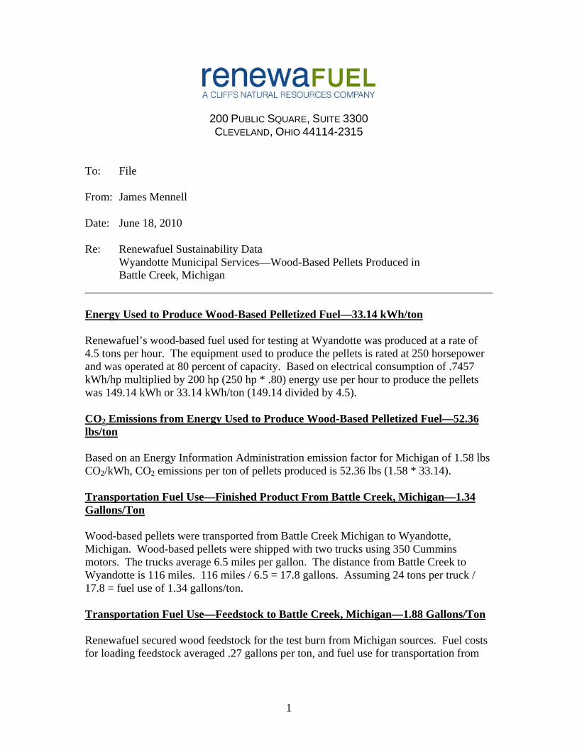
200 PUBLIC SQUARE, SUITE 3300 CLEVELAND, OHIO 44114-2315
To: File From: James Mennell Date: June 18, 2010 Re: Renewafuel Sustainability Data Wyandotte Municipal Services—Wood-Based Pellets Produced in
Battle Creek, Michigan ________________________________________________________________________ Energy Used to Produce Wood-Based Pelletized Fuel—33.14 kWh/ton Renewafuel’s wood-based fuel used for testing at Wyandotte was produced at a rate of 4.5 tons per hour. The equipment used to produce the pellets is rated at 250 horsepower and was operated at 80 percent of capacity. Based on electrical consumption of .7457 kWh/hp multiplied by 200 hp (250 hp * .80) energy use per hour to produce the pellets was 149.14 kWh or 33.14 kWh/ton (149.14 divided by 4.5). CO2 Emissions from Energy Used to Produce Wood-Based Pelletized Fuel—52.36 lbs/ton Based on an Energy Information Administration emission factor for Michigan of 1.58 lbs CO2/kWh, CO2 emissions per ton of pellets produced is 52.36 lbs (1.58 * 33.14). Transportation Fuel Use—Finished Product From Battle Creek, Michigan—1.34 Gallons/Ton Wood-based pellets were transported from Battle Creek Michigan to Wyandotte, Michigan. Wood-based pellets were shipped with two trucks using 350 Cummins motors. The trucks average 6.5 miles per gallon. The distance from Battle Creek to Wyandotte is 116 miles. 116 miles / 6.5 = 17.8 gallons. Assuming 24 tons per truck / 17.8 = fuel use of 1.34 gallons/ton. Transportation Fuel Use—Feedstock to Battle Creek, Michigan—1.88 Gallons/Ton Renewafuel secured wood feedstock for the test burn from Michigan sources. Fuel costs for loading feedstock averaged .27 gallons per ton, and fuel use for transportation from
1

suppliers to Battle Creek averaged 1.61 gallons per ton. Total fuel for loading and transporting feedstock to Battle Creek averaged 1.88 gallons per ton. CO2 Emissions From Transportation Fuel Use—63 lbs/Ton (total), 36.8 lbs/Ton for Feedstock to Battle Creek and 26.2 lb/ton for Finished Product to Wyandotte Based on an Energy Information Administration emission factor of 19.564 lbs CO2/gallon, CO2 emissions per ton of finished pellets transported from Battle Creek to Wyandotte are 26.2 lbs (1.34 * 19.564). CO2 emissions per ton of feedstock transported to Battle Creek are 36.8 lbs (1.88 * 19.564). Total CO2 from transportation of feedstock to Battle Creek and finished product from Battle Creek to Wyandotte is 63 lbs/ton. CO2 Emissions from Combustion of Bituminous Coal Compared to Wood Pellets Based on an Energy Information Administration emission factor bituminous coal (currently used at Wyandotte) results in CO2 emissions of 4,931.30 lbs/ton. Combustion of Renewafuel wood pellets, which are comprised of biogenic carbon—meaning it is part of the natural carbon balance and will not add to atmospheric concentrations of CO2--emits no creditable CO2 emissions under international greenhouse gas accounting methods developed by the Intergovernmental Panel on Climate Change. Carbon Balance of Renewafuel Wood-Based Fuel Compared to Bituminous Coal—Coal Emits More than 40 times More CO2 than Renewafuel Wood-Based Fuel CO2 Emitting Activity Renewafuel Wood-Based
Fuel Bituminous Coal
Mining 0 ? Methane Releases 0 ? Processing 52 lbs/ton ? Transportation 63 lbs/ton ? Use as Fuel at Wyandotte 0/ton 4,931 lbs/ton TOTAL 115 lbs/ton 4,931 lbs/ton (+ mining,
methane releases, processing and transportation)
Even without considering the CO2 emissions from mining, methane releases, processing and transporting coal to Wyandotte, CO2 emissions from use of coal are roughly 40 times higher than use of Renewafuel’s wood-based fuel (even when considering all emissions from processing and transportation of the wood-based fuel). Energy Equivalent CO2 Emission Reductions of renewaFUEL Compared to Bituminous Coal—1.58 tons of CO2/Ton of renewaFUEL Assuming and average heating value of 8,000 Btu/lb for renewaFUEL and 12,500 Btu/lb for bituminous coal, a ton of renewaFUEL has 64% of the energy value of a ton of
2

3
bituminous coal. Multiplying the EIA emission factor for bituminous coal of CO2 emissions of 4,931.30 lbs/ton by .64 equals 3,156 lbs of CO2 (1.58 tons) from such coal on an energy-equivalent basis to one ton of renewaFUEL. Use of 30,000 Tons of renewaFUEL in Place of Bituminous Coal Would Reduce Creditable CO2 Emissions By the Equivalent of the Annual Use of 8,000 Cars Assuming an offset of 1.58 tons of CO2 per ton of renewaFUEL used in place of bituminous coal, and use of 30,000 tons of renewaFUEL, would result in reductions of 47,400 tons of CO2. A typical car emits 0.916 lbs of CO2 per mile. Assuming average annual use of 12,500 miles per year, a typical car would emit 11,450 lbs (5.73 tons) of CO2 per year. Dividing annual creditable CO2 reductions of 47,400 by 5.73 indicates use of 30,000 tons of renewaFUEL would result in creditable CO2 reductions equivalent to the annual use of 8,272 cars.

N. Robert Froese Traverse City Presentation
Traverse CityBiomass FuelsAssessment
Robert Froese, PhD, RPFAssociate Professor ofForest Resources and Environmental Science
with contributions from
Stacie Holmes, Nan Davisand Trevor Roberts
Traverse City Light & Power Information Session
21 January 2010 at Traverse City, MICopyright © 2010 – Robert E. Froese. All rights reserved.
Context for this Study
• TCL&P is exploring opportunities for biomass-fueled Combined Heat and Power
• One or more 10 MW plants, total up to 40 MW
• Consider a range of fuels, including forestry residuals, energy crops and wood by barge
• Information needed on fuel properties, availability within a feasible procurement range, and expected biomass cost
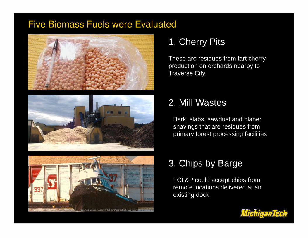
1. Cherry Pits
These are residues from tart cherry production on orchards nearby to Traverse City
2. Mill Wastes
Bark, slabs, sawdust and planer shavings that are residues from primary forest processing facilities
3. Chips by Barge
TCL&P could accept chips from remote locations delivered at an existing dock
Five Biomass Fuels were Evaluated
http://i.pbase.com/v3/29/593629/1/50330819.Haulingchipbargeout.jpg
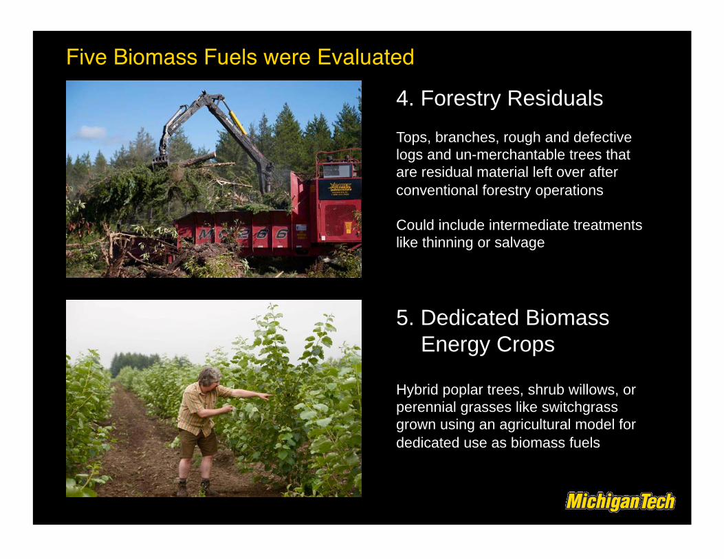
4. Forestry Residuals
Tops, branches, rough and defective logs and un-merchantable trees that are residual material left over after conventional forestry operations
Could include intermediate treatments like thinning or salvage
5. Dedicated Biomass Energy Crops
Hybrid poplar trees, shrub willows, or perennial grasses like switchgrass grown using an agricultural model for dedicated use as biomass fuels
Five Biomass Fuels were Evaluated
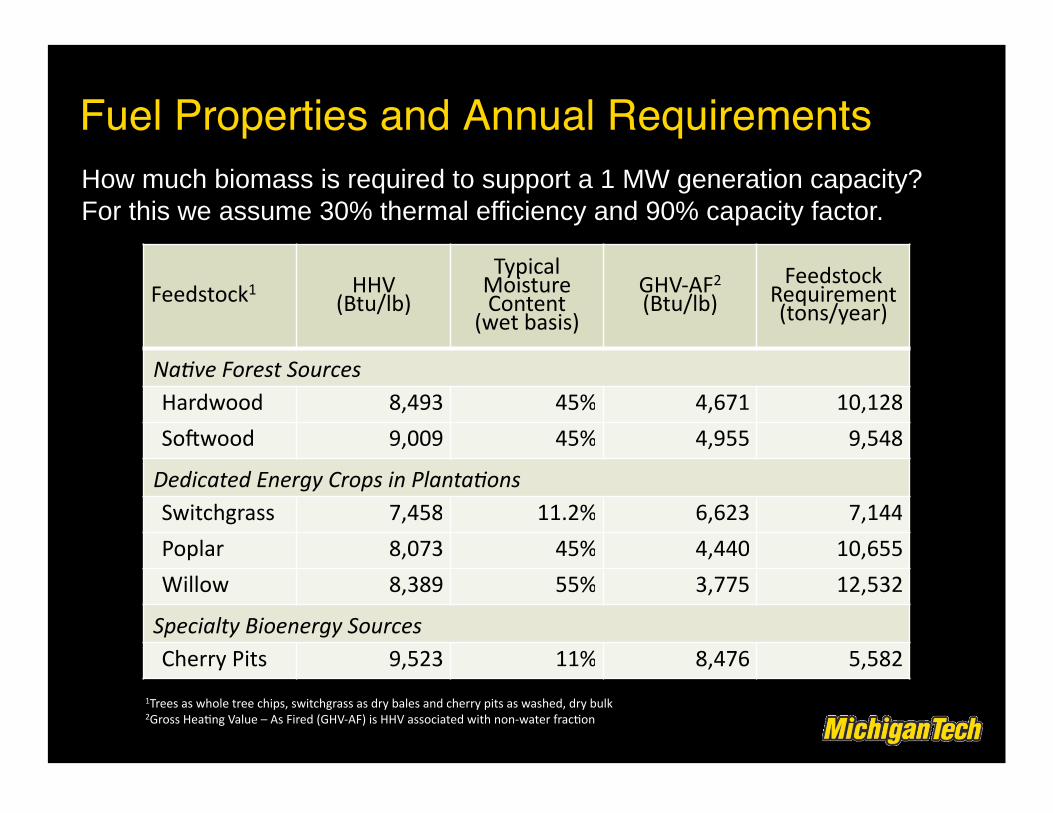
Fuel Properties and Annual Requirements
How much biomass is required to support a 1 MW generation capacity? For this we assume 30% thermal efficiency and 90% capacity factor.

Scope - Geography
We established a reference “bioshed” with a radius of 75 miles from Traverse City
The bioshed is divided into bands to impose some spatial context for subsequent analyses.
Bands are progressively thinner as they are further from Traverse City. This means each band is roughly equal in area.

Land Cover
Within 75 miles of Traverse City
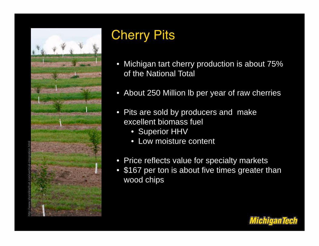
Cherry Pitsht
tp://
ww
w.s
hore
linef
ruit.
com
/ver
tical
-inte
grat
ion.
htm
l
• Michigan tart cherry production is about 75% of the National Total
• About 250 Million lb per year of raw cherries
• Pits are sold by producers and make excellent biomass fuel
• Superior HHV • Low moisture content
• Price reflects value for specialty markets • $167 per ton is about five times greater than
wood chips

Wood Chips by Bargeht
tp://
i.pba
se.c
om/v
3/29
/593
629/
1/50
3308
19.H
aulin
gchi
pbar
geou
t.jpg
• Michigan has 38 deep-water ports, 15 of which are on Lake Michigan
• Barge transportation is very efficient • Fuel efficiency is 5 times greater than rail
and 10 times greater than truck
• Barge loads are large; typical barge displaces 3,400 tons
• Barge movement could be seasonal
• Little chip movement at present

Mill Wastes are Already Utilized
Mill Wastes
1. USDA Timber Products Output
• Mill survey • Estimates of removals
and residues estimated backwards
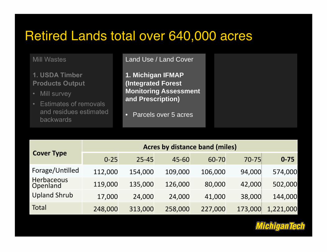
Mill Wastes
1. USDA Timber Products Output
• Mill survey • Estimates of removals
and residues estimated backwards
Land Use / Land Cover
1. Michigan IFMAP (Integrated Forest Monitoring Assessment and Prescription)
• Parcels over 5 acres
Retired Lands total over 640,000 acres
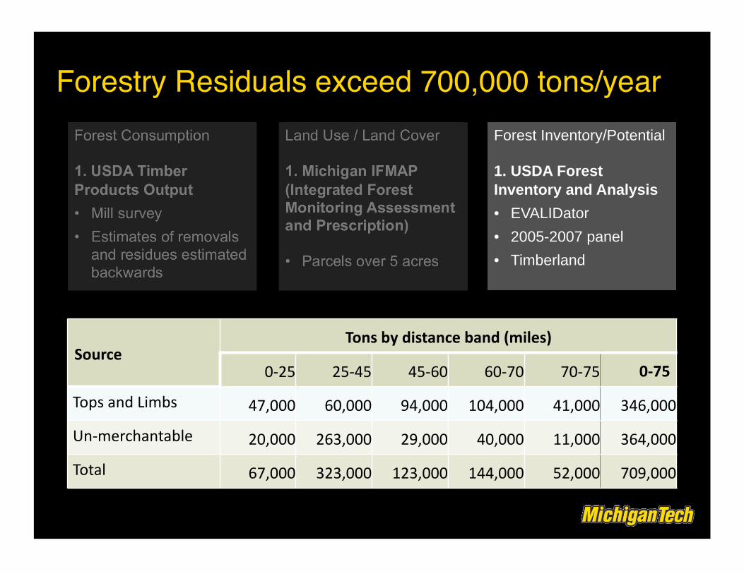
Forestry Residuals exceed 700,000 tons/year
Forest Consumption
1. USDA Timber Products Output
• Mill survey • Estimates of removals
and residues estimated backwards
Forest Inventory/Potential
1. USDA Forest Inventory and Analysis
• EVALIDator • 2005-2007 panel • Timberland
Land Use / Land Cover
1. Michigan IFMAP (Integrated Forest Monitoring Assessment and Prescription)
• Parcels over 5 acres

Forest have large renewable energy potential
Annual Change Million
ft3Million
tons1Current rate of harvest of forest resources may be estimated very accurately using inventory data collected by the USDA Forest Service
Harvest is presently about 30% of growth. In other words, 70% of growth is accumulating as new inventory, year after year.
Harvest rate could be doubled and still be less than the sustainable rate. Associated residues would be substantial.

1. Shrub Willow
• High-density plantations using clonal cuttings on cultivated lands
• Cut every 3 years for 7-8 cycles • Most expensive option
2. Hybrid Poplar • Low-density plantations using clonal
cuttings; cultivation optional • Harvested on a 10-year rotation • Commercial experience elsewhere in
the Upper Midwest
3. Switchgrass
• Native warm-season grass • Annual harvest after fall frost • Reaches full yield in 2-4 years • Least expensive option
Dedicated Biomass Energy Crops

Feasible Availability Scenario
1. Existing Timber Harvest
Associated with existing harvest of logs are about 700,000 green tons/year of forestry residuals, after deducting a retention requirement for sustainability. Some of these residues are collected and used already. About 40% might be available at Traverse City.
2. New Sustainable Timber Harvest
At present, forest harvest is only 30% of forest growth and a very large potential exists for increased sustainable timber harvest. The Michigan Climate Action Council scenario assumed some new harvest could be diverted to bioenergy. If the current harvest rate were increased by 20% (i.e., from 30% of growth to 36% of growth), then about 240,000 green tons/year of low-grade logs and residuals might be available at Traverse City.
3. Dedicated Energy Crops from Retired Farmland
There are about 640,000 acres of apparently idle, retired farmlands within 75-miles of Traverse City. If TCL&P could contract for energy crop production on 20% of these lands, all of the biomass under these contracts (about 5.5 green tons/acre/year) might be available at Traverse City.
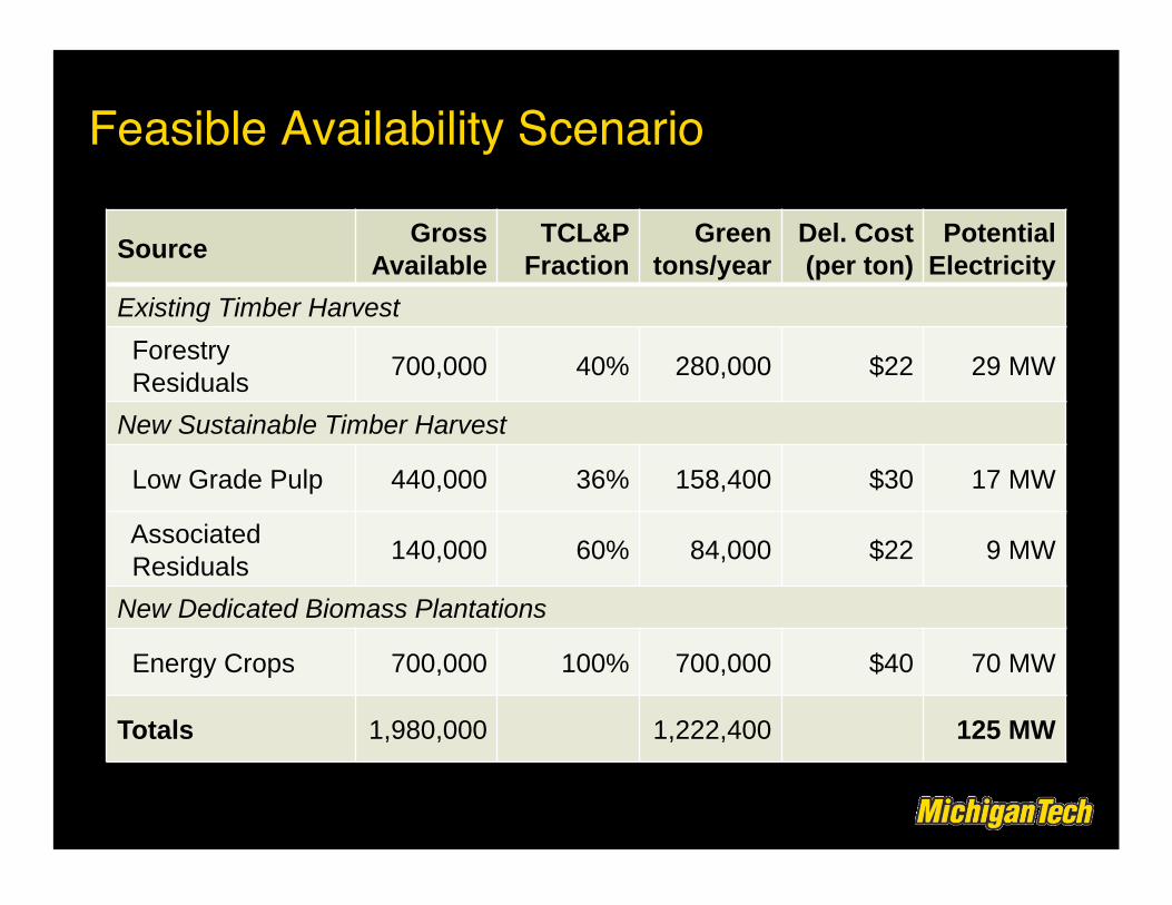
Source Gross
AvailableTCL&P
FractionGreen
tons/year Del. Cost(per ton)
PotentialElectricity
Existing Timber Harvest
Forestry Residuals 700,000 40% 280,000 $22 29 MW
New Sustainable Timber Harvest
Low Grade Pulp 440,000 36% 158,400 $30 17 MW
Associated Residuals 140,000 60% 84,000 $22 9 MW
New Dedicated Biomass Plantations
Energy Crops 700,000 100% 700,000 $40 70 MW
Totals 1,980,000 1,222,400 125 MW
Feasible Availability Scenario

O. Sawmill Operations Serving Southeastern Michigan

The Southeast Michigan RC&D Council is an equal opportunity provider and employer. Inclusion on this list does not imply endorsement of any specific businesses and does not guarantee that listings are current.
Thanks to the Washtenaw Conservation District for providing much of the information on this list.
Small and Portable Sawmill Operations Serving Southeastern Michigan
Ace Sawmill Portable sawmill 17416 Savage Rd Belleville, MI 48111 Ph: (734) 635-3333 E-mail: [email protected] Blue Ox Mill Works Portable sawmill Richard Russo 8673 W. Iosco Fowlerville, MI 48836 Ph: (517) 223-7268 Boston Lumber Ray Peltier 5903 State Road Fort Gratiot, MI 48059 Ph: (810) 650-1901 E-mail: [email protected] Dan Erickson Portable sawmill 1960 Miller Ave. Ann Arbor, MI 48103 Ph: (734) 668-0885 Fx: (734) 647-2767 Don Brown Portable sawmill 504 Diamond Rd. Mason, MI 48854-8604 Ph: (517) 676-4487 Freier Forestry P.O. Box 130710 Ann Arbor, MI 48113 Ph: (734) 320-2770, (734) 323-0027 E-mail: [email protected] http://www.freierforestryllc.com/ Gary Flint Custom sawmill, blade sharpening 11205 Orban Road Grass Lake, MI 49240-9809 Ph: (517) 522-3337
G&D Lumber Portable sawmill 12860 S. Hillsdale Rd. Camden, MI 49232 Ph: (517) 254-4463 Approx 100 Mile radius J&E Services John Zempke Portable sawmill P.O. Box 834 Lakeland, MI 48143 Ph: (810) 231-9389 J&W Tree Artisans Tree removal & milling services Wayne Nemeth 54445 Bates Chesterfield Twp., MI 48051 Ph: (586)749-8672 John Haling Portable sawmill, Kiln drying 6559 Nollar Rd. Whitmore Lake, MI 48189 Ph: (734) 741-9499 Fx: (734) 741-9498 http://www.sawmilljohn.com/ Joseph Zalac Portable sawmill 5125 Whitlow Ct. Commerce Township, MI 48382 Ph: (248) 363-6521 Hobbyist Hickory & Oak Sawmilling Portable Sawmill, Kiln Drying Steve Van Osdol
90930 52nd
St. Decatur, MI 49045 Ph: (269) 423-8178 Kevin Bingham Detroit, MI Ph: (313) 319-0583
Krupa's Custom Cutting Sawmill owner, custom cutting, kiln 7607 South Huron River Drive South Rockwood, MI 48179 Ph: (734) 379-3120 E-mail: [email protected] http://www.krupascustomcutting.com Last Chance Logs to Lumber Portable sawmill Chris Last 9971 Cardwell Livonia, MI 48150 Ph: (734) 261-0441 Cell: (734) 564-4705 E-mail: [email protected] Log 2 Lumber Chuck Lobaito Farmington Hills, MI Ph: (248) 330-9033 E-mail: [email protected] http://log2lumber.googlepages.com/ Logs to Lumber and Beyond Richard Mills Flat Rock, MI 48134 Ph: (734) 231-1210 [email protected] http://www.logstolumberandbeyond.com/ Looking North Wood Products Steve & Dawn Wilson operators 901 W State Street St. Johns, MI 48879 Ph: (989) 224-6725 Cell: (989)-640-1505 [email protected] MDJZ Custom Cutting Portable sawmill Steve Mixter 7180 Pounds Ct. Howell, MI 48855 Ph: (517) 546-6558
7203 Jackson Road Ann Arbor MI 48103-9506
Phone: (734) 761-6722 X 105 Fax: (734) 662-1686 Web Site: www.semircd.org
Serving Lenawee, Macomb, Monroe, Oakland,
St. Clair, Washtenaw and Wayne Counties

The Southeast Michigan RC&D Council is an equal opportunity provider and employer. Inclusion on this list does not imply endorsement of any specific businesses and does not guarantee that listings are current.
Thanks to the Washtenaw Conservation District for providing much of the information on this list.
Meinert's Mill Jim Meinert 7431 Lulu Rd Petersburg, MI Ph: (734) 279-2306 Metro Portable Sawmill Portable Sawmill, Kiln Drying Mike Carter 20241 Coryell Dr. Beverly Hills, MI 48025 Ph: (248) 563-3881 Mobile Custom Sawing Robert Dewitt 10498 Ostrander Rd. Maybee, MI 48159 Ph: (734) 604-3604 Fx: (734) 587-3222 Also sells lumber Pete Klink Forestry Consultant, Kiln Drying P.O. Box 521 Coldwater, MI 49036 Ph: (517) 238-4048 Quinn Mobile Saw Works LLC Martin Quinn 38321 Chartier Harrison Twp., MI 48045 Ph: (231) 557-7271 E-mail: [email protected] http://q-saw.com/ Raven Farm 7535 Clark Rd. Bath, MI 48808 Ph: (517) 641-6189 Email: [email protected] http://www.ravenfarm.com/ Rusty 4 Farms Portable sawmill, Kiln Drying, Firewood 27190 L Drive North Albion, MI 49224 Ph: (517) 629-9218 Cell: (231) 206-4381 Sawing Logz LLC Portable sawmill, Firewood Jeff Shelby 28634 Milton Ave. Warren, MI 48092 Ph: (586) 883-5649
Sawmill Express Portable sawmill Manchester, MI Ph: (734) 428-7975 Mike Weber - Ph: (734) 368-5914 Dave Kirk - Ph: (734) 216-6061 Scotty's Custom Sawing and Millwork Portable sawmill, millwork, Firewood Scott Tupacz Belleville, MI Ph: (734) 461-2133 Fx: (734) 787-8295 Tervol Wood Products Portable sawmill, Kiln drying 11800 N. Adams Rd. North Adams, MI 49262 Ph: (517) 287-5745 Pallet and Container Corp. of America Portable sawmill, Pallet lumber buyer Todd Burtscher 901 Buckingham St. Toledo, Oh 43607 Ph: (419) 255-1256 - Shop Fx: (419) 255-1257 Fax Cell: (419) 344-3920 - best # to use E-mail: [email protected] Ullmann Urban Sawmill Lee Ullmann Dexter, MI Ph: (734)253-2585 Lon Ullmann Troy, MI Ph: (248)670-6875 http://uusaw.com/ Urbanwood.org Sawmill services and online store Cooperative network of many local mills Retail sales at: Recycle Ann Arbor’s ReUse Center 2420 South Industrial Hwy. Ann Arbor, MI Ph: (734) 222-7880 http://urbanwood.org/
Variety Farms Sawmill Portable mill, “Buyer of quality sawlogs” Robert Bullock 11585 Dunham Rd. Hartland, MI 48353 Ph: (810) 623-0041 Walton’s Portable Sawmill Portable Sawmill, Kiln Drying Eric Walton 863 Hazelwood Jackson, MI 49203 Ph: (517) 795-7815 You can also find more wood products businesses online at the MI Department of Natural Resources’ Wood Products Directory: http://www.michigandnr.com/wood/.

P. Test Burn PI and CEMS Data
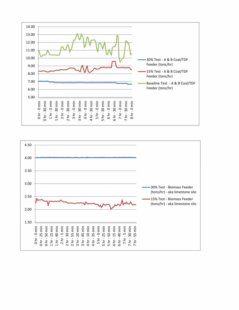
5.00
6.00
7.00
8.00
9.00
10.00
11.00
12.00
13.00
14.00
0 hr ‐0 min
0 hr ‐30
min
1 hr ‐0 min
1 hr ‐30
min
2 hr ‐0 min
2 hr ‐30
min
3 hr ‐0 min
3 hr ‐30
min
4 hr ‐0 min
4 hr ‐30
min
5 hr ‐0 min
5 hr ‐30
min
6 hr ‐0 min
6 hr ‐30
min
7 hr ‐0 min
7 hr ‐30
min
8 hr ‐0 min
30% Test ‐ A & B Coal/TDF Feeder (tons/hr)
15% Test ‐ A & B Coal/TDF Feeder (tons/hr)
Baseline Test ‐ A & B Coal/TDF Feeder (tons/hr)
4.00
4.50
5.00
6.00
7.00
8.00
9.00
10.00
11.00
12.00
13.00
14.00
0 hr ‐0 min
0 hr ‐30
min
1 hr ‐0 min
1 hr ‐30
min
2 hr ‐0 min
2 hr ‐30
min
3 hr ‐0 min
3 hr ‐30
min
4 hr ‐0 min
4 hr ‐30
min
5 hr ‐0 min
5 hr ‐30
min
6 hr ‐0 min
6 hr ‐30
min
7 hr ‐0 min
7 hr ‐30
min
8 hr ‐0 min
30% Test ‐ A & B Coal/TDF Feeder (tons/hr)
15% Test ‐ A & B Coal/TDF Feeder (tons/hr)
Baseline Test ‐ A & B Coal/TDF Feeder (tons/hr)
1.50
2.00
2.50
3.00
3.50
4.00
4.50
0 hr ‐0 min
0 hr ‐25
min
0 hr ‐50
min
1 hr ‐15
min
1 hr ‐40
min
2 hr ‐5 min
2 hr ‐30
min
2 hr ‐55
min
3 hr ‐20
min
3 hr ‐45
min
4 hr ‐10
min
4 hr ‐35
min
5 hr ‐0 min
5 hr ‐25
min
5 hr ‐50
min
6 hr ‐15
min
6 hr ‐40
min
7 hr ‐5 min
7 hr ‐30
min
7 hr ‐55
min
30% Test ‐ Biomass Feeder (tons/hr) ‐ aka limestone silo
15% Test ‐ Biomass Feeder (tons/hr) ‐ aka limestone silo
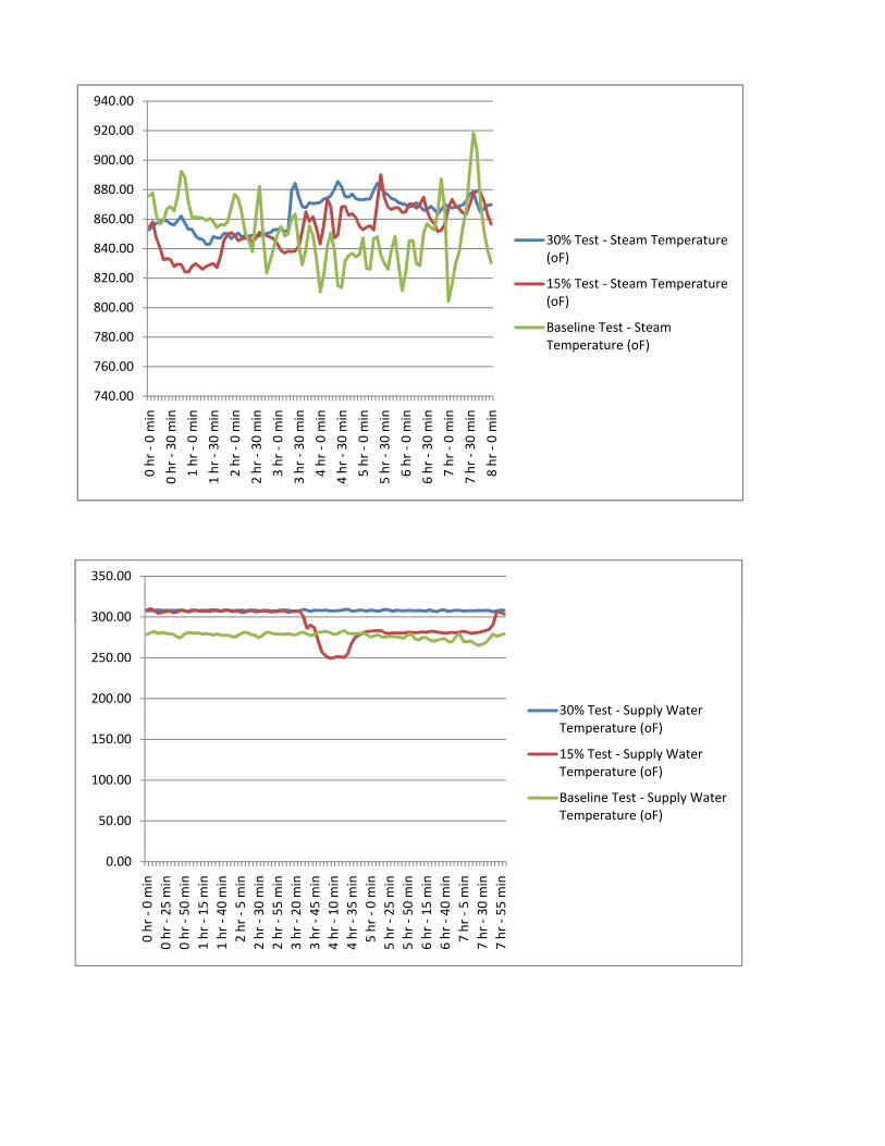
740.00
760.00
780.00
800.00
820.00
840.00
860.00
880.00
900.00
920.00
940.00
0 hr ‐0 min
0 hr ‐30
min
1 hr ‐0 min
1 hr ‐30
min
2 hr ‐0 min
2 hr ‐30
min
3 hr ‐0 min
3 hr ‐30
min
4 hr ‐0 min
4 hr ‐30
min
5 hr ‐0 min
5 hr ‐30
min
6 hr ‐0 min
6 hr ‐30
min
7 hr ‐0 min
7 hr ‐30
min
8 hr ‐0 min
30% Test ‐ Steam Temperature (oF)
15% Test ‐ Steam Temperature (oF)
Baseline Test ‐ Steam Temperature (oF)
300.00
350.00
740.00
760.00
780.00
800.00
820.00
840.00
860.00
880.00
900.00
920.00
940.00
0 hr ‐0 min
0 hr ‐30
min
1 hr ‐0 min
1 hr ‐30
min
2 hr ‐0 min
2 hr ‐30
min
3 hr ‐0 min
3 hr ‐30
min
4 hr ‐0 min
4 hr ‐30
min
5 hr ‐0 min
5 hr ‐30
min
6 hr ‐0 min
6 hr ‐30
min
7 hr ‐0 min
7 hr ‐30
min
8 hr ‐0 min
30% Test ‐ Steam Temperature (oF)
15% Test ‐ Steam Temperature (oF)
Baseline Test ‐ Steam Temperature (oF)
0.00
50.00
100.00
150.00
200.00
250.00
300.00
350.00
0 hr ‐0 min
0 hr ‐25
min
0 hr ‐50
min
1 hr ‐15
min
1 hr ‐40
min
2 hr ‐5 min
2 hr ‐30
min
2 hr ‐55
min
3 hr ‐20
min
3 hr ‐45
min
4 hr ‐10
min
4 hr ‐35
min
5 hr ‐0 min
5 hr ‐25
min
5 hr ‐50
min
6 hr ‐15
min
6 hr ‐40
min
7 hr ‐5 min
7 hr ‐30
min
7 hr ‐55
min
30% Test ‐ Supply Water Temperature (oF)
15% Test ‐ Supply Water Temperature (oF)
Baseline Test ‐ Supply Water Temperature (oF)

0
50
100
150
200
250
300
0 hr ‐ 0 min
0 hr ‐ 30 min
1 hr ‐ 0 min
1 hr ‐ 30 min
2 hr ‐ 0 min
2 hr ‐ 30 min
3 hr ‐ 0 min
3 hr ‐ 30 min
4 hr ‐ 0 min
4 hr ‐ 30 min
5 hr ‐ 0 min
5 hr ‐ 30 min
6 hr ‐ 0 min
6 hr ‐ 30 min
7 hr ‐ 0 min
7 hr ‐ 30 min
8 hr ‐ 0 min
30% Test ‐ SO2 PPM
15% Test ‐ SO2 PPM
Baseline Test ‐ SO2 PPM
130
135
140
0
50
100
150
200
250
300
0 hr ‐ 0 min
0 hr ‐ 30 min
1 hr ‐ 0 min
1 hr ‐ 30 min
2 hr ‐ 0 min
2 hr ‐ 30 min
3 hr ‐ 0 min
3 hr ‐ 30 min
4 hr ‐ 0 min
4 hr ‐ 30 min
5 hr ‐ 0 min
5 hr ‐ 30 min
6 hr ‐ 0 min
6 hr ‐ 30 min
7 hr ‐ 0 min
7 hr ‐ 30 min
8 hr ‐ 0 min
30% Test ‐ SO2 PPM
15% Test ‐ SO2 PPM
Baseline Test ‐ SO2 PPM
90
95
100
105
110
115
120
125
130
135
140
0 hr ‐ 0 min
0 hr ‐ 30 min
1 hr ‐ 0 min
1 hr ‐ 30 min
2 hr ‐ 0 min
2 hr ‐ 30 min
3 hr ‐ 0 min
3 hr ‐ 30 min
4 hr ‐ 0 min
4 hr ‐ 30 min
5 hr ‐ 0 min
5 hr ‐ 30 min
6 hr ‐ 0 min
6 hr ‐ 30 min
7 hr ‐ 0 min
7 hr ‐ 30 min
8 hr ‐ 0 min
30% Test ‐ Nox PPM
15% Test ‐ Nox PPM
Baseline Test ‐ Nox PPM
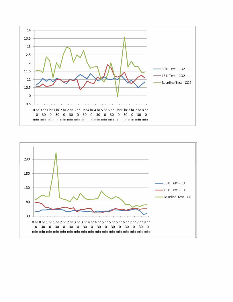
230
9.5
10
10.5
11
11.5
12
12.5
13
13.5
14
0 hr ‐ 0 min
0 hr ‐ 30 min
1 hr ‐ 0 min
1 hr ‐ 30 min
2 hr ‐ 0 min
2 hr ‐ 30 min
3 hr ‐ 0 min
3 hr ‐ 30 min
4 hr ‐ 0 min
4 hr ‐ 30 min
5 hr ‐ 0 min
5 hr ‐ 30 min
6 hr ‐ 0 min
6 hr ‐ 30 min
7 hr ‐ 0 min
7 hr ‐ 30 min
8 hr ‐ 0 min
30% Test ‐ CO2
15% Test ‐ CO2
Baseline Test ‐ CO2
30
80
130
180
230
0 hr ‐ 0 min
0 hr ‐ 30 min
1 hr ‐ 0 min
1 hr ‐ 30 min
2 hr ‐ 0 min
2 hr ‐ 30 min
3 hr ‐ 0 min
3 hr ‐ 30 min
4 hr ‐ 0 min
4 hr ‐ 30 min
5 hr ‐ 0 min
5 hr ‐ 30 min
6 hr ‐ 0 min
6 hr ‐ 30 min
7 hr ‐ 0 min
7 hr ‐ 30 min
8 hr ‐ 0 min
30% Test ‐ CO
15% Test ‐ CO
Baseline Test ‐ CO
9.5
10
10.5
11
11.5
12
12.5
13
13.5
14
0 hr ‐ 0 min
0 hr ‐ 30 min
1 hr ‐ 0 min
1 hr ‐ 30 min
2 hr ‐ 0 min
2 hr ‐ 30 min
3 hr ‐ 0 min
3 hr ‐ 30 min
4 hr ‐ 0 min
4 hr ‐ 30 min
5 hr ‐ 0 min
5 hr ‐ 30 min
6 hr ‐ 0 min
6 hr ‐ 30 min
7 hr ‐ 0 min
7 hr ‐ 30 min
8 hr ‐ 0 min
30% Test ‐ CO2
15% Test ‐ CO2
Baseline Test ‐ CO2
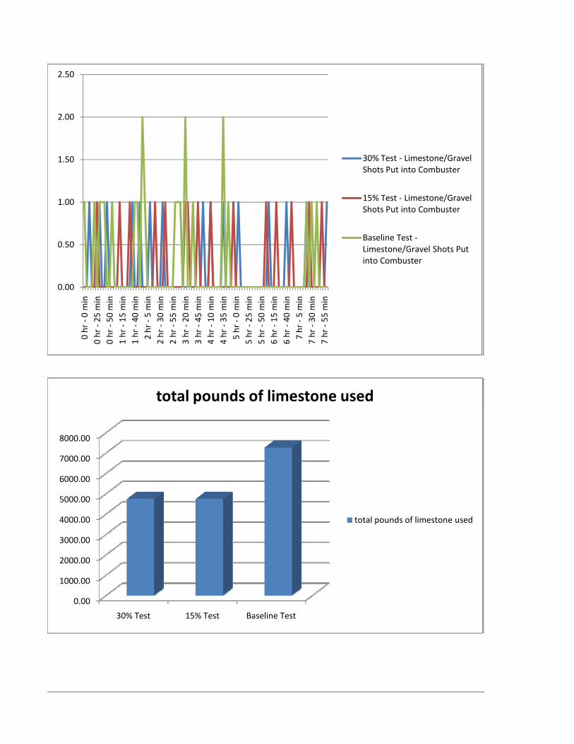
0.00
0.50
1.00
1.50
2.00
2.500 hr ‐0 min
0 hr ‐25
min
0 hr ‐50
min
1 hr ‐15
min
1 hr ‐40
min
2 hr ‐5 min
2 hr ‐30
min
2 hr ‐55
min
3 hr ‐20
min
3 hr ‐45
min
4 hr ‐10
min
4 hr ‐35
min
5 hr ‐0 min
5 hr ‐25
min
5 hr ‐50
min
6 hr ‐15
min
6 hr ‐40
min
7 hr ‐5 min
7 hr ‐30
min
7 hr ‐55
min
30% Test ‐ Limestone/Gravel Shots Put into Combuster
15% Test ‐ Limestone/Gravel Shots Put into Combuster
Baseline Test ‐Limestone/Gravel Shots Put into Combuster
total pounds of limestone used
0.00
0.50
1.00
1.50
2.00
2.500 hr ‐0 min
0 hr ‐25
min
0 hr ‐50
min
1 hr ‐15
min
1 hr ‐40
min
2 hr ‐5 min
2 hr ‐30
min
2 hr ‐55
min
3 hr ‐20
min
3 hr ‐45
min
4 hr ‐10
min
4 hr ‐35
min
5 hr ‐0 min
5 hr ‐25
min
5 hr ‐50
min
6 hr ‐15
min
6 hr ‐40
min
7 hr ‐5 min
7 hr ‐30
min
7 hr ‐55
min
30% Test ‐ Limestone/Gravel Shots Put into Combuster
15% Test ‐ Limestone/Gravel Shots Put into Combuster
Baseline Test ‐Limestone/Gravel Shots Put into Combuster
0.00
1000.00
2000.00
3000.00
4000.00
5000.00
6000.00
7000.00
8000.00
30% Test 15% Test Baseline Test
total pounds of limestone used
total pounds of limestone used

0.00
0.00
0.00
0.00
0.00
0.01
0.01
0.01
0 hr ‐0 min
0 hr ‐25
min
0 hr ‐50
min
1 hr ‐15
min
1 hr ‐40
min
2 hr ‐5 min
2 hr ‐30
min
2 hr ‐55
min
3 hr ‐20
min
3 hr ‐45
min
4 hr ‐10
min
4 hr ‐35
min
5 hr ‐0 min
5 hr ‐25
min
5 hr ‐50
min
6 hr ‐15
min
6 hr ‐40
min
7 hr ‐5 min
7 hr ‐30
min
7 hr ‐55
min
30% Test ‐ Attemperator Flow
15% Test ‐ Attemperator Flow
Baseline Test ‐ Attemperator Flow
185
0.00
0.00
0.00
0.00
0.00
0.01
0.01
0.01
0 hr ‐0 min
0 hr ‐25
min
0 hr ‐50
min
1 hr ‐15
min
1 hr ‐40
min
2 hr ‐5 min
2 hr ‐30
min
2 hr ‐55
min
3 hr ‐20
min
3 hr ‐45
min
4 hr ‐10
min
4 hr ‐35
min
5 hr ‐0 min
5 hr ‐25
min
5 hr ‐50
min
6 hr ‐15
min
6 hr ‐40
min
7 hr ‐5 min
7 hr ‐30
min
7 hr ‐55
min
30% Test ‐ Attemperator Flow
15% Test ‐ Attemperator Flow
Baseline Test ‐ Attemperator Flow
160
165
170
175
180
185
0 hr ‐0 min
0 hr ‐25
min
0 hr ‐50
min
1 hr ‐15
min
1 hr ‐40
min
2 hr ‐5 min
2 hr ‐30
min
2 hr ‐55
min
3 hr ‐20
min
3 hr ‐45
min
4 hr ‐10
min
4 hr ‐35
min
5 hr ‐0 min
5 hr ‐25
min
5 hr ‐50
min
6 hr ‐15
min
6 hr ‐40
min
7 hr ‐5 min
7 hr ‐30
min
7 hr ‐55
min
30% Test ‐ Flue Gas Temp in oF
15% Test ‐ Flue Gas Temp in oF
Baseline Test ‐ Flue Gas Temp in oF

1400
1450
1500
1550
1600
16500 hr ‐0 min
0 hr ‐25
min
0 hr ‐50
min
1 hr ‐15
min
1 hr ‐40
min
2 hr ‐5 min
2 hr ‐30
min
2 hr ‐55
min
3 hr ‐20
min
3 hr ‐45
min
4 hr ‐10
min
4 hr ‐35
min
5 hr ‐0 min
5 hr ‐25
min
5 hr ‐50
min
6 hr ‐15
min
6 hr ‐40
min
7 hr ‐5 min
7 hr ‐30
min
7 hr ‐55
min
30% Test ‐ Combustion Air Temp oF
15% Test ‐ Combustion Air Temp oF
Baseline Test ‐ Combustion Air Temp oF

185.00190.00195.00200.00205.00210.00
650.00
700.00
750.00
800.00
850.00
900.00
950.00
1000.00
0 hr ‐0 min
0 hr ‐30
min
1 hr ‐0 min
1 hr ‐30
min
2 hr ‐0 min
2 hr ‐30
min
3 hr ‐0 min
3 hr ‐30
min
4 hr ‐0 min
4 hr ‐30
min
5 hr ‐0 min
5 hr ‐30
min
6 hr ‐0 min
6 hr ‐30
min
7 hr ‐0 min
7 hr ‐30
min
8 hr ‐0 min
30% Test ‐ Steam Pressure (psig)
15% Test ‐ Steam Pressure (psig)
Baseline Test ‐ Steam Pressure (psig)
120.00125.00130.00135.00140.00145.00150.00155.00160.00165.00170.00175.00180.00185.00190.00195.00200.00205.00210.00
0 hr ‐0 min
0 hr ‐25
min
0 hr ‐50
min
1 hr ‐15
min
1 hr ‐40
min
2 hr ‐5 min
2 hr ‐30
min
2 hr ‐55
min
3 hr ‐20
min
3 hr ‐45
min
4 hr ‐10
min
4 hr ‐35
min
5 hr ‐0 min
5 hr ‐25
min
5 hr ‐50
min
6 hr ‐15
min
6 hr ‐40
min
7 hr ‐5 min
7 hr ‐30
min
7 hr ‐55
min
30% Test ‐ Steam Flow (Thousand lb/hr)
15% Test ‐ Steam Flow (Thousand lb/hr)
Baseline Test ‐ Steam Flow (Thousand lb/hr)
650.00
700.00
750.00
800.00
850.00
900.00
950.00
1000.00
0 hr ‐0 min
0 hr ‐30
min
1 hr ‐0 min
1 hr ‐30
min
2 hr ‐0 min
2 hr ‐30
min
3 hr ‐0 min
3 hr ‐30
min
4 hr ‐0 min
4 hr ‐30
min
5 hr ‐0 min
5 hr ‐30
min
6 hr ‐0 min
6 hr ‐30
min
7 hr ‐0 min
7 hr ‐30
min
8 hr ‐0 min
30% Test ‐ Steam Pressure (psig)
15% Test ‐ Steam Pressure (psig)
Baseline Test ‐ Steam Pressure (psig)
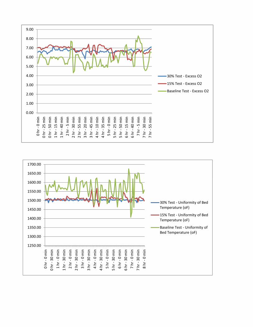
0.00
1.00
2.00
3.00
4.00
5.00
6.00
7.00
8.00
9.00
0 hr ‐0 min
0 hr ‐25
min
0 hr ‐50
min
1 hr ‐15
min
1 hr ‐40
min
2 hr ‐5 min
2 hr ‐30
min
2 hr ‐55
min
3 hr ‐20
min
3 hr ‐45
min
4 hr ‐10
min
4 hr ‐35
min
5 hr ‐0 min
5 hr ‐25
min
5 hr ‐50
min
6 hr ‐15
min
6 hr ‐40
min
7 hr ‐5 min
7 hr ‐30
min
7 hr ‐55
min
30% Test ‐ Excess O2
15% Test ‐ Excess O2
Baseline Test ‐ Excess O2
1650.00
1700.00
0.00
1.00
2.00
3.00
4.00
5.00
6.00
7.00
8.00
9.00
0 hr ‐0 min
0 hr ‐25
min
0 hr ‐50
min
1 hr ‐15
min
1 hr ‐40
min
2 hr ‐5 min
2 hr ‐30
min
2 hr ‐55
min
3 hr ‐20
min
3 hr ‐45
min
4 hr ‐10
min
4 hr ‐35
min
5 hr ‐0 min
5 hr ‐25
min
5 hr ‐50
min
6 hr ‐15
min
6 hr ‐40
min
7 hr ‐5 min
7 hr ‐30
min
7 hr ‐55
min
30% Test ‐ Excess O2
15% Test ‐ Excess O2
Baseline Test ‐ Excess O2
1250.00
1300.00
1350.00
1400.00
1450.00
1500.00
1550.00
1600.00
1650.00
1700.00
0 hr ‐0 min
0 hr ‐30
min
1 hr ‐0 min
1 hr ‐30
min
2 hr ‐0 min
2 hr ‐30
min
3 hr ‐0 min
3 hr ‐30
min
4 hr ‐0 min
4 hr ‐30
min
5 hr ‐0 min
5 hr ‐30
min
6 hr ‐0 min
6 hr ‐30
min
7 hr ‐0 min
7 hr ‐30
min
8 hr ‐0 min
30% Test ‐ Uniformity of Bed Temperature (oF)
15% Test ‐ Uniformity of Bed Temperature (oF)
Baseline Test ‐ Uniformity of Bed Temperature (oF)
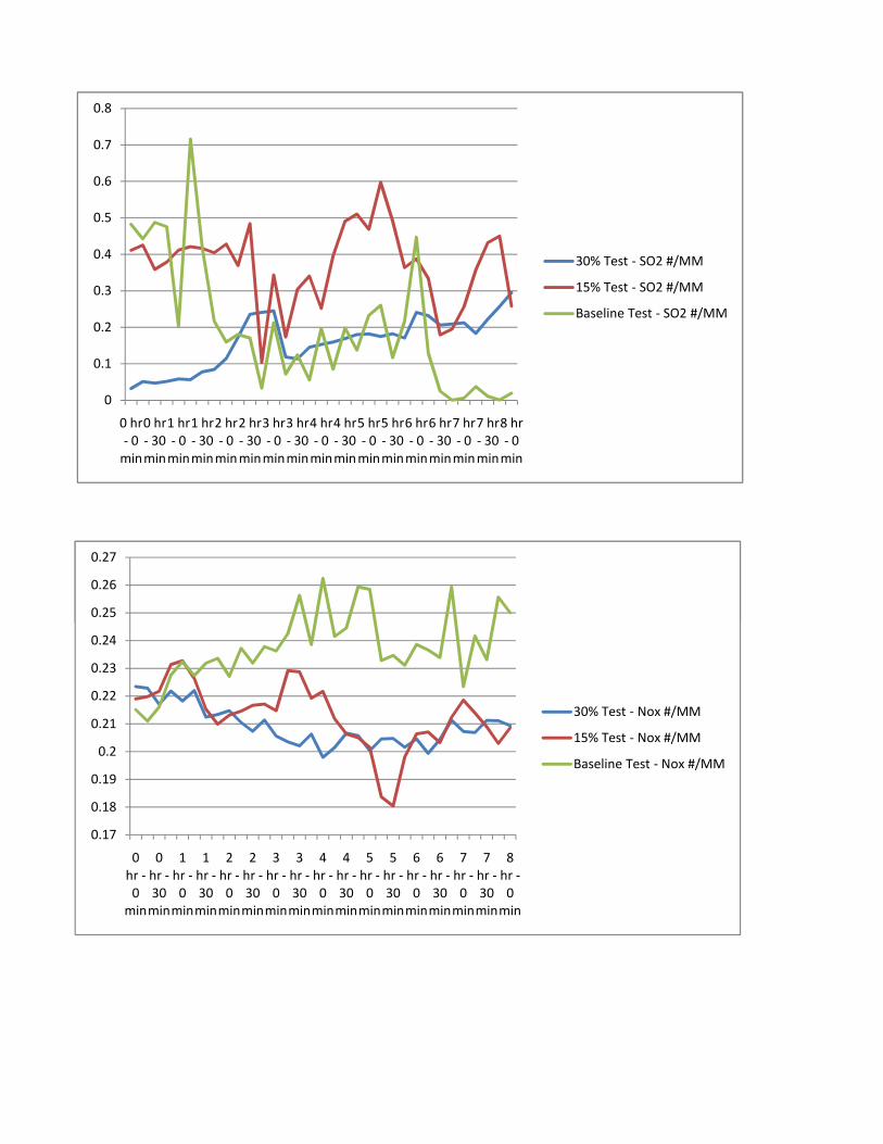
0
0.1
0.2
0.3
0.4
0.5
0.6
0.7
0.8
0 hr ‐ 0 min
0 hr ‐ 30 min
1 hr ‐ 0 min
1 hr ‐ 30 min
2 hr ‐ 0 min
2 hr ‐ 30 min
3 hr ‐ 0 min
3 hr ‐ 30 min
4 hr ‐ 0 min
4 hr ‐ 30 min
5 hr ‐ 0 min
5 hr ‐ 30 min
6 hr ‐ 0 min
6 hr ‐ 30 min
7 hr ‐ 0 min
7 hr ‐ 30 min
8 hr ‐ 0 min
30% Test ‐ SO2 #/MM
15% Test ‐ SO2 #/MM
Baseline Test ‐ SO2 #/MM
0.25
0.26
0.27
0
0.1
0.2
0.3
0.4
0.5
0.6
0.7
0.8
0 hr ‐ 0 min
0 hr ‐ 30 min
1 hr ‐ 0 min
1 hr ‐ 30 min
2 hr ‐ 0 min
2 hr ‐ 30 min
3 hr ‐ 0 min
3 hr ‐ 30 min
4 hr ‐ 0 min
4 hr ‐ 30 min
5 hr ‐ 0 min
5 hr ‐ 30 min
6 hr ‐ 0 min
6 hr ‐ 30 min
7 hr ‐ 0 min
7 hr ‐ 30 min
8 hr ‐ 0 min
30% Test ‐ SO2 #/MM
15% Test ‐ SO2 #/MM
Baseline Test ‐ SO2 #/MM
0.17
0.18
0.19
0.2
0.21
0.22
0.23
0.24
0.25
0.26
0.27
0 hr ‐0
min
0 hr ‐30 min
1 hr ‐0
min
1 hr ‐30 min
2 hr ‐0
min
2 hr ‐30 min
3 hr ‐0
min
3 hr ‐30 min
4 hr ‐0
min
4 hr ‐30 min
5 hr ‐0
min
5 hr ‐30 min
6 hr ‐0
min
6 hr ‐30 min
7 hr ‐0
min
7 hr ‐30 min
8 hr ‐0
min
30% Test ‐ Nox #/MM
15% Test ‐ Nox #/MM
Baseline Test ‐ Nox #/MM

750.00
800.00
850.00
900.00
950.00
1000.00
1050.00
0 hr ‐0 min
0 hr ‐25
min
0 hr ‐50
min
1 hr ‐15
min
1 hr ‐40
min
2 hr ‐5 min
2 hr ‐30
min
2 hr ‐55
min
3 hr ‐20
min
3 hr ‐45
min
4 hr ‐10
min
4 hr ‐35
min
5 hr ‐0 min
5 hr ‐25
min
5 hr ‐50
min
6 hr ‐15
min
6 hr ‐40
min
7 hr ‐5 min
7 hr ‐30
min
7 hr ‐55
min
30% Test ‐ Supply Water Pressure (psig)
15% Test ‐ Supply Water Pressure (psig)
Baseline Test ‐ Supply Water Pressure (psig)
2 4
2.6
2.8
3
750.00
800.00
850.00
900.00
950.00
1000.00
1050.00
0 hr ‐0 min
0 hr ‐25
min
0 hr ‐50
min
1 hr ‐15
min
1 hr ‐40
min
2 hr ‐5 min
2 hr ‐30
min
2 hr ‐55
min
3 hr ‐20
min
3 hr ‐45
min
4 hr ‐10
min
4 hr ‐35
min
5 hr ‐0 min
5 hr ‐25
min
5 hr ‐50
min
6 hr ‐15
min
6 hr ‐40
min
7 hr ‐5 min
7 hr ‐30
min
7 hr ‐55
min
30% Test ‐ Supply Water Pressure (psig)
15% Test ‐ Supply Water Pressure (psig)
Baseline Test ‐ Supply Water Pressure (psig)
1
1.2
1.4
1.6
1.8
2
2.2
2.4
2.6
2.8
3
0 hr ‐0 min
0 hr ‐25
min
0 hr ‐50
min
1 hr ‐15
min
1 hr ‐40
min
2 hr ‐5 min
2 hr ‐30
min
2 hr ‐55
min
3 hr ‐20
min
3 hr ‐45
min
4 hr ‐10
min
4 hr ‐35
min
5 hr ‐0 min
5 hr ‐25
min
5 hr ‐50
min
6 hr ‐15
min
6 hr ‐40
min
7 hr ‐5 min
7 hr ‐30
min
7 hr ‐55
min
30% Test ‐West Cyclone Pressure Drop (psig)
15% Test ‐West Cyclone Pressure Drop (psig)
Baseline Test ‐West Cyclone Pressure Drop (psig)
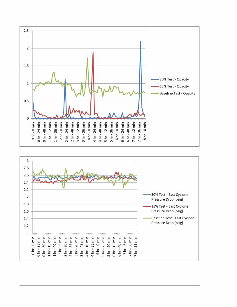
0
0.5
1
1.5
2
2.50 hr ‐0 min
0 hr ‐24
min
0 hr ‐48
min
1 hr ‐12
min
1 hr ‐36
min
2 hr ‐0 min
2 hr ‐24
min
2 hr ‐48
min
3 hr ‐12
min
3 hr ‐36
min
4 hr ‐0 min
4 hr ‐24
min
4 hr ‐48
min
5 hr ‐12
min
5 hr ‐36
min
6 hr ‐0 min
6 hr ‐24
min
6 hr ‐48
min
7 hr ‐12
min
7 hr ‐36
min
8 hr ‐0 min
30% Test ‐ Opacity
15% Test ‐ Opacity
Baseline Test ‐ Opacity
2 8
3
0
0.5
1
1.5
2
2.50 hr ‐0 min
0 hr ‐24
min
0 hr ‐48
min
1 hr ‐12
min
1 hr ‐36
min
2 hr ‐0 min
2 hr ‐24
min
2 hr ‐48
min
3 hr ‐12
min
3 hr ‐36
min
4 hr ‐0 min
4 hr ‐24
min
4 hr ‐48
min
5 hr ‐12
min
5 hr ‐36
min
6 hr ‐0 min
6 hr ‐24
min
6 hr ‐48
min
7 hr ‐12
min
7 hr ‐36
min
8 hr ‐0 min
30% Test ‐ Opacity
15% Test ‐ Opacity
Baseline Test ‐ Opacity
1
1.2
1.4
1.6
1.8
2
2.2
2.4
2.6
2.8
3
0 hr ‐0 min
0 hr ‐25
min
0 hr ‐50
min
1 hr ‐15
min
1 hr ‐40
min
2 hr ‐5 min
2 hr ‐30
min
2 hr ‐55
min
3 hr ‐20
min
3 hr ‐45
min
4 hr ‐10
min
4 hr ‐35
min
5 hr ‐0 min
5 hr ‐25
min
5 hr ‐50
min
6 hr ‐15
min
6 hr ‐40
min
7 hr ‐5 min
7 hr ‐30
min
7 hr ‐55
min
30% Test ‐ East Cyclone Pressure Drop (psig)
15% Test ‐ East Cyclone Pressure Drop (psig)
Baseline Test ‐ East Cyclone Pressure Drop (psig)

90
95
100
105
110
115
120
0 hr ‐0 min
0 hr ‐25
min
0 hr ‐50
min
1 hr ‐15
min
1 hr ‐40
min
2 hr ‐5 min
2 hr ‐30
min
2 hr ‐55
min
3 hr ‐20
min
3 hr ‐45
min
4 hr ‐10
min
4 hr ‐35
min
5 hr ‐0 min
5 hr ‐25
min
5 hr ‐50
min
6 hr ‐15
min
6 hr ‐40
min
7 hr ‐5 min
7 hr ‐30
min
7 hr ‐55
min
30% Test ‐ Intake Air Temp oF
15% Test ‐ Intake Air Temp oF
Baseline Test ‐ Intake Air Temp oF
320
90
95
100
105
110
115
120
0 hr ‐0 min
0 hr ‐25
min
0 hr ‐50
min
1 hr ‐15
min
1 hr ‐40
min
2 hr ‐5 min
2 hr ‐30
min
2 hr ‐55
min
3 hr ‐20
min
3 hr ‐45
min
4 hr ‐10
min
4 hr ‐35
min
5 hr ‐0 min
5 hr ‐25
min
5 hr ‐50
min
6 hr ‐15
min
6 hr ‐40
min
7 hr ‐5 min
7 hr ‐30
min
7 hr ‐55
min
30% Test ‐ Intake Air Temp oF
15% Test ‐ Intake Air Temp oF
Baseline Test ‐ Intake Air Temp oF
275
280
285
290
295
300
305
310
315
320
0 hr ‐0 min
0 hr ‐25
min
0 hr ‐50
min
1 hr ‐15
min
1 hr ‐40
min
2 hr ‐5 min
2 hr ‐30
min
2 hr ‐55
min
3 hr ‐20
min
3 hr ‐45
min
4 hr ‐10
min
4 hr ‐35
min
5 hr ‐0 min
5 hr ‐25
min
5 hr ‐50
min
6 hr ‐15
min
6 hr ‐40
min
7 hr ‐5 min
7 hr ‐30
min
7 hr ‐55
min
30% Test ‐ Flue Gas Temp out oF
15% Test ‐ Flue Gas Temp out oF
Baseline Test ‐ Flue Gas Temp out oF
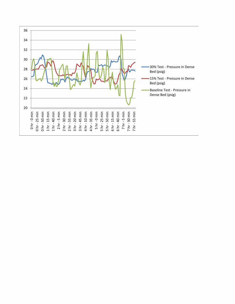
20
22
24
26
28
30
32
34
360 hr ‐0 min
0 hr ‐25
min
0 hr ‐50
min
1 hr ‐15
min
1 hr ‐40
min
2 hr ‐5 min
2 hr ‐30
min
2 hr ‐55
min
3 hr ‐20
min
3 hr ‐45
min
4 hr ‐10
min
4 hr ‐35
min
5 hr ‐0 min
5 hr ‐25
min
5 hr ‐50
min
6 hr ‐15
min
6 hr ‐40
min
7 hr ‐5 min
7 hr ‐30
min
7 hr ‐55
min
30% Test ‐ Pressure in Dense Bed (psig)
15% Test ‐ Pressure in Dense Bed (psig)
Baseline Test ‐ Pressure in Dense Bed (psig)

Q. Test Burn Procedure

1
Table of Contents 1 Overview ............................................................................................................................................... 2
2 Responsibilities ..................................................................................................................................... 2
3 Test Burn Monitoring Parameters ........................................................................................................ 3
4 Proposed Tests – Durations and Biomass Tonnages ............................................................................ 4
5 Fuel Handling Procedures ..................................................................................................................... 6
6 Pre‐test Check List ................................................................................................................................. 6
7 Data Collection ...................................................................................................................................... 7
8 Results and Data Compilation ............................................................................................................... 8
9 Daily Log ................................................................................................................................................ 9
10 Test Burn Completion Field Meeting .................................................................................................... 9
Appendix A – Boiler Operator Test Log Form
Appendix B – Fuel Sample Log Form
Appendix C – Boiler Operator Visual Record
Appendix D – Pre‐Test Checklist

2
1 Overview This test burn procedure is designed to evaluate boiler performance when co‐firing clean extruded wood
biomass with coal in the Wyandotte Municipal Services (WMS) Unit #8 Boiler. This test burn will
evaluate co‐firing WMS’s normal 60/40 blend of PRB Coal/TDF fuel with renewaFUEL’s clean extruded
one hundred percent wood biomass product.
Changes in operational performance with regard to efficiency, emissions, and fly ash characteristics will
be evaluated while combusting one‐hundred percent PRB coal/TDF and then reevaluated while co‐firing
biomass with PRB coal/TDF at steady state conditions (steam flow and fuel mixtures) in multiple ratios.
The following general testing approach will be followed:
1) Perform Baseline test with 60/40 blend of PRB Coal/TDF fuel.
2) Collect performance data under (a) typical operating mode and (b) while burning a blend of
coal/TDF and the wood biomass fuel.
3) Analyze the test results to evaluate changes in boiler emissions performance attributable to
wood biomass co‐firing.
The baseline test will be completed one to two weeks prior to the renewaFUEL biomass test burns to
provide an opportunity to test the data collection procedures with the controller’s, operators, and field
personnel who will complete the work.
2 Responsibilities A representative of Barr/ WMS will coordinate testing activities with the boiler operators to confirm that
all testing is conducted at the desired boiler operating set points and the boiler operational data needed
to calculate efficiency is properly logged and stored. Barr will supervise the field testing activities. Daily
log forms attached in appendices will be used to document test periods and conditions.
Barr will plan and manage the following aspects of the test burn:
1) Confirming that sufficient uniform source of wood biomass is available for testing
2) Scheduling of test activities to minimize impact on site operations
3) Identifying safe access to the test location
4) Coordinating subcontractors and analytical laboratories

3
WMS will be responsible for any procedure that is associated with Unit #8 normal operations including
but not limited to:
1) Fuel storage site preparation
2) Fuel conveyance
3) Boiler operations
4) Equipment operations
5) Visual recording of combustion zone
6) Fuel sampling at gravimetric feeders
7) Data collection using existing CEMS, DCS and PI systems
3 Test Burn Monitoring Parameters Specifically, the operating points tested will be: the boiler firing PRB coal/TDF only at a typical steam
capacity, of 180,000 lb/Hr and the boiler firing wood biomass/PRB Coal/TDF mixture at its normal fuel
blend at the same operating load. By limiting the testing to normal operational points, the approach
minimizes the chance of other operational changes within the boiler from masking the effect of co‐
firing.
The verification parameters listed below will be evaluated. This list was developed based on project
objectives cited by the client.
1) Boiler efficiency during biomass co‐firing and normalize emissions to boiler output
2) Changes in emissions
a. Nitrogen oxides (NOx)
b. Sulfur dioxide (SO2)
c. Carbon monoxide (CO)
d. Carbon dioxide (CO2)
e. Total particulates (TPM),via opacity
3) Changes in fly ash characteristics including:
a. Carbon, hydrogen, and nitrogen (CHN), and minerals content
b. Primary metals: arsenic (As), selenium (Se), zinc (Zn), and mercury (Hg)
c. Secondary metals: barium (Ba), beryllium (Be), cadmium (Cd), chromium (Cr), copper
(Cu), manganese (Mn), nickel (Ni), and silver (Ag)
d. Potential boiler fouling components: calcium (Ca), sodium (Na), and potassium (K)
e. Fly ash fusion temperature
f. RCRA metals TCLP
g. Air entraining agent index
Boiler efficiency will be observed using WMS Digital Control Systems (DCS) screen shots during the
baseline test and then calculated with the PI historian software data collected during the baseline test.
The same process of using the PI historian software data collection and the DCS screen shots will be

4
completed during the biomass test burn conditions. The observations and calculated data will then be
compared to one another to determine if the boiler efficiency was altered during the biomass testing.
Boiler efficiency parameters:
1) Intake air temperature, oF
2) Flue gas temperature at air heater inlet and outlet, oF
3) Fuel temperature, oF
4) Moisture in air, lb/lb dry air
5) Fuel consumption, lb/hr
6) Combustion air temperature, oF
7) Steam flow, MMBtu/h or lb/h
8) Steam pressure, psig
9) Steam temperature, oF
10) Supply water pressure, psig 11) Supply water temperature, oF
12) Power generation, kW
13) Fuel ultimate analyses, both wood and coal
14) Fuel heating value, Btu/lb 15) Unburned carbon loss, % 16) Excess O2 or air
The primary focus of each biomass test burn is to monitor the boiler output of the test materials to
determine boiler capacity. Fan horse power and air/flue gas flows will also be monitored to aid in
determining biomass boiler capacity.
A verbal record of the operating stability will be documented along with a steam pressure plot to
determine the operating stability differences during the baseline test and the biomass test burns.
The following items will be monitored to help determine the bed operations during the baseline test and
also the biomass test burns.
1) Screen shot data
2) Bed temperature
3) Uniformity of bed temps
4) Pressure drop – air and flue gas
5) Visual observations of the bed
6) Functioning of the external heat exchanger
7) Bed inventory
4 Proposed Tests – Durations and Biomass Tonnages
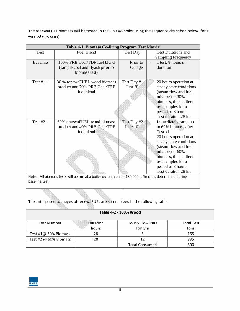
5
The renewaFUEL biomass will be tested in the Unit #8 boiler using the sequence described below (for a
total of two tests).
Table 4-1 Biomass Co-firing Program Test Matrix Test Fuel Blend Test Day Test Durations and
Sampling Frequency Baseline 100% PRB Coal/TDF fuel blend
(sample coal and flyash prior to biomass test)
Prior to Outage
- 1 test, 8 hours in duration
Test #1 – 30 % renewaFUEL wood biomass product and 70% PRB Coal/TDF
fuel blend
Test Day #1 June 8th
- 20 hours operation at steady state conditions (steam flow and fuel mixture) at 30% biomass, then collect test samples for a period of 8 hours
- Test duration 28 hrs Test #2 – 60% renewaFUEL wood biomass
product and 40% PRB Coal/TDF fuel blend
Test Day #2 June 10th
- Immediately ramp up to 60% biomass after Test #1
- 20 hours operation at steady state conditions (steam flow and fuel mixture) at 60% biomass, then collect test samples for a period of 8 hours
- Test duration 28 hrs Note: All biomass tests will be run at a boiler output goal of 180,000 lb/hr or as determined during baseline test.
The anticipated tonnages of renewaFUEL are summarized in the following table.
Table 4‐2 ‐ 100% Wood
Test Number
Duration hours
Hourly Flow Rate Tons/hr
Total Test tons
Test #1@ 30% Biomass 28 6 165
Test #2 @ 60% Biomass 28 12 335
Total Consumed 500

6
All testing will be conducted during steady state boiler operations (steam flow and fuel mixture). Test
and sampling procedures will be as consistent as possible between sets of tests. Any problems occurred
during testing will be recorded to help define anomalies.
5 Fuel Handling Procedures Prior to delivery of the biomass fuel, WMS will empty the Unit #8 limestone silo. The biomass will be
stored in the Unit #8 limestone silo for the duration of the testing.
Prior to conveying the biomass fuel into the Unit #8 limestone silo, WMS will clear the reclaim area and
also clear the belts.
The renewaFUEL product will be delivered via 35 ton truck. The trucks will use a walking bed to unload
fuel into the WMS coal yard. The biomass fuel will be dumped onto the Unit #8 Grizzly and fed into the
reclaim. The fuel will be delivered via the Unit #8 Reclaim onto the Unit #8 conveyer to the Unit #8
limestone silo. The Unit #8 limestone silo will be filled with 100% biomass, approximately 84 tons
capacity. The Unit #8 bunker will be filled with the normal 60/40 blend of PRB Coal/TDF fuel. The
biomass feed rate will be controlled by the existing gravimetric feeder.
Delivery of the biomass will be coordinated to meet the requirements of the two tests described in
Table 4‐1. The limestone silo will need to be filled several times during each test.
After the test burns are completed the boiler and fuel handling equipment will be positioned for normal
operating conditions.
6 Pre‐test Check List Boiler operations verifying the following shall be completed by the WMS boiler operators prior to each
test burn.
1) Boiler is operating at 180,000 lb/hr
2) Bed operation is stable
3) Boiler is stable
4) No coal feeder issues
5) No boiler feed pump issues
6) Control room operator is ready for test
7) Shift supervisor is ready and located where needed
8) Correct fuel is located in the correct bunkers for fuel feed
9) Computer system is up and running
10) All data to be collected is being recorded 11) Existing baghouse has one hopper emptied to ensure PRB Coal/TDF fly ash is not included in fly
ash sampling
7
12) Fuel handling system is clean of all PRB Coal/TDF fuel to ensure an accurate reading of the
biomass test burn emissions
13) Staff are in the correct location and prepared to complete their assigned tasks
7 Data Collection The following DCS data points will be collected using the PI Historian software system which allows the
facility to customize data acquisition, storage, and reporting activities. The boiler is also equipped with
continuous emission monitoring systems (CEMS) that record NOx, SO2, CO, and Ox concentrations and
emission rates.
Operation parameters that will be recorded during this test program include the following:
1) Intake air temperature, oF
2) Flue gas temperature at air heater inlet and outlet, oF
3) Fuel temperature, oF (manually with a heat gun)
4) Fuel consumption, lb/hr
5) Combustion air temperature, oF
6) Steam flow, MMBtu/h or lb/h
7) Steam pressure, psig
8) Steam temperature, oF
9) Supply water pressure, psig
10) Supply water temperature, oF
11) Power generation, kW
12) Fuel ultimate analyses, both wood and coal
13) Fuel heating value, Btu/lb 14) Unburned carbon loss, % 15) Excess O2 or air
16) Power output (MW)
17) Heat input for coal, wood, and total, (Btu/hr) 18) Coal and wood feed rates via belt scales, (lb/hr) 19) Emissions
a. Nitrogen oxides (NOx), CEM
b. Sulfur dioxide (SO2), CEM
c. Carbon monoxide (CO)
d. Carbon dioxide (CO2), CEM
e. Total particulates (TPM), via opacity
20) Multiclone pressure drop (in w.c.)
21) Bed temperature
22) Uniformity of bed temps
23) Pressure drop across the bed 24) Visual observations of the bed
8
25) Functioning of the external heat exchanger 26) Visual observation of fugitive dust
These data points will be collected on a five minute basis during the baseline test and for the each
biomass test burn and exported to an excel spreadsheet.
Fuel samples will be taken from the gravimetric feeders for the 100% renewaFUEL clean extruded wood
biomass product and the PRB Coal/TDF fuel blend. The samples will be taken on 30 minute intervals,
marked with the date and time taken, sealed and sent to an independent testing facility.
A flyash sample will need to be collected at the completion of each test. Prior to starting the biomass
test burns the baghouse dust collection hoppers shall be emptied. This will ensure that a representative
sample for the biomass test burn is collected. At the completion of each test burn a flyash sample shall
be collected.
8 Results and Data Compilation Upon completion of testing the following data compilation will be performed. The results will be
presented in a final report completed by Barr.
At the conclusion of field testing, results will be analyzed to evaluate changes in boiler performance, fly
ash characteristics, and to verify the statistical significance of any observed changed in emissions or
efficiency between tests and renewaFUEL products.
Data recorded on each test period will be averaged over the test period and reported to document
boiler operations during the testing, co‐firing rates, and boiler efficiency.
The ultimate analysis will report the following fuel constituents as percent by weight:
1) Carbon
2) BTU
3) Water/Moisture
4) Ash
5) Sulfur
6) Hydrogen
7) Oxygen
8) Nitrogen
9) Fines/Including wood species
The fly ash samples will be sent to a lab for testing of the following changes in fly ash characteristics
including:
1) Carbon, hydrogen, and nitrogen (CHN), and minerals content

9
2) Primary metals: arsenic (As), selenium (Se), zinc (Zn), and mercury (Hg)
3) Secondary metals: barium (Ba), beryllium (Be), cadmium (Cd), chromium (Cr), copper (Cu),
manganese (Mn), nickel (Ni), and silver (Ag)
4) Potential boiler fouling components: calcium (Ca), sodium (Na), and potassium (K)
5) Fly ash fusion temperature
6) RCRA metals TCLP
7) Air entraining agent index
9 Daily Log The following daily logs will be recorded for each test.
The boiler operator will be responsible for the log attached form located in appendix A.
The visual observations of how the biomass fuel is delivering into boiler, confirmation the boiler is
operating correctly, record of any operating problems that have occurred prior to test, and also view
port recordings will be completed by experienced WMS on‐site staff for each test and recorded on the
attached form located in appendix B.
The Pre‐test checklist attached in appendix C will be completed by WMS staff prior to each test.
A fuel sample log form will be completed every 30 minutes by WMS staff during each test
10 Test Burn Completion Field Meeting Immediately following each test, a meeting will be held to collect the log sheets, fuel samples and record
comments from the biomass testing and any observations made by the testing personnel. A thorough
review of any record of operating problems will be reviewed along with any fuel handling concerns, such
as, whether WMS had to poke the bunker to get the fuel to flow at any point during testing or if the
boiler output goal of 180,000 lb/hr deviated during the test cycle.
Upon completion of the biomass testing the required activities to switch back to normal PRB Coal/TDF
operation will begin, by WMS. Barr will remain on‐site to observe and confirm the change over from
biomass to PRB Coal/TDF is seamless and also be available to help resolve issues as they may occur.

10
���������

11
WYANDOTTE MUNICPAL SERVICES
UNIT # 8 renewaFUEL BIOMASS TEST BURN
BOILER OPERATOR TEST LOG FORM
Project ID: ______________________________ Date:___________________________________
Unit Description:_________________________ Signature:_______________________________
Test Description:_________________________ Test No.:_______________________________
_______________________________________ Clock Synch performed (Initials):_____________
Start
½ hr
1 hr
1 ½ hr
2 hr
2 ½ hr
3 hr
3 ½ hr
4 hr
4 ½ hr
5 hr
5 ½ hr
6 hr
6 ½ hr
7 hr
7 ½ hr
End
Time
Biomass Blend Rate, %
Steam Flow, lb/hr
Steam Pressure @ boiler outlet,
psig
Steam Temperature @ boiler outlet,
oF
Combustion Air Temp.,
oF (downstream of air heater)
Ambient Air Temp., oF
(upstream of air heater)
Generating Rate, kW
Notes:

12
��������

13
WYANDOTTE MUNICPAL SERVICES
UNIT # 8 renewaFUEL BIOMASS TEST BURN
FUEL SAMPLE LOG FORM
Project ID: ______________________________ Date:___________________________________
Unit Description:_________________________ Signature:_______________________________
Test Description:_________________________ Test No.:_______________________________
_______________________________________ Clock Synch performed (Initials):_____________
Biomass Sample
Start ½ hr
1 hr
1 ½ hr
2 hr
2 ½ hr
3 hr
3 ½ hr
4 hr
4 ½ hr
5 hr
5 ½ hr
6 hr
6 ½ hr
7 hr
7 ½ hr
End
Time
Quantity
Initials of Sampler
PRB Coal/TDF Sample
Start ½ hr
1 hr
1 ½ hr
2 hr
2 ½ hr
3 hr
3 ½ hr
4 hr
4 ½ hr
5 hr
5 ½ hr
6 hr
6 ½ hr
7 hr
7 ½ hr
End
Time
Quantity
Initials of Sampler
Ash Sample Start End
Time
Quantity
Initials of Sampler
Notes:

14
���������

15
WYANDOTTE MUNICPAL SERVICES
UNIT # 8 renewaFUEL BIOMASS TEST BURN
BOILER OPERATOR VISUAL RECORD
Project ID: ______________________________ Date:___________________________________
Unit Description:_________________________ Signature:_______________________________
Test Description:_________________________ Test No.:_______________________________
_______________________________________ Clock Synch performed (Initials):_____________
Operating Problems Occurring Prior Test:
Fuel Delivery Visual Observations:
Boiler Operation Notes:
Boiler Bed Notes:
Operating Problems Occurring During Test:
Other Notes:
*VISUAL OBSERVATIONS TO BE RECORDED EACH HOUR OF TESTING

16
���������

17
WYANDOTTE MUNICPAL SERVICES
UNIT # 8 renewaFUEL BIOMASS TEST BURN
PRE‐TEST CHECKLIST
Project ID: ______________________________ Date:___________________________________
Unit Description:_________________________ Signature:_______________________________
Test Description:_________________________ Test No.:_______________________________
_______________________________________ Clock Synch performed (Initials):_____________
Boiler is operating at 160,000 lb/Hr
Bed operation is stable
Boiler is stable
No coal feeder issues
No boiler feed pump issues
Control room operator is ready for test
Shift supervisor is ready and located where needed
Correct fuel is located in the correct bunkers for fuel feed
Computer system is up and running, both PI and CEM’s
All data to be collected is being recorded
Existing baghouse has one hopper emptied to ensure PRB Coal/TDF fly ash is not included in fly ash
Sampling
Staff are in the correct location and prepared to complete their assigned tasks

R. Traverse City Report

Business Confidential
Integrated Resource Plan Traverse City Light and Power
February 2010


Business Confidential
Integrated Resource Plan Traverse City Light and Power
February 2010

This report has been prepared for the use of the client for the specific purposes identified in the report. The conclusions, observations and recommendations contained herein attributed to R. W. Beck, Inc. (R. W. Beck) constitute the opinions of R. W. Beck. To the extent that statements, information and opinions provided by the client or others have been used in the preparation of this report, R. W. Beck has relied upon the same to be accurate, and for which no assurances are intended and no representations or warranties are made. R. W. Beck makes no certification and gives no assurances except as explicitly set forth in this report.
Copyright 2010, R. W. Beck, Inc. All rights reserved.

R:\Orlando\010633 - Traverse City\05-01528-20101 IRP\Work Products\Draft_2010\TCLP IRP Report_FINAL.docx
Integrated Resource Plan Traverse City Light and Power
Table of Contents
Executive Summary
Section 1 INTRODUCTION .................................................................................... 1-1 1.1 Study Purpose .......................................................................................... 1-1 1.2 Overview of TCLP ................................................................................... 1-2 1.3 Overview of the MISO East Market ........................................................ 1-3 1.4 General Study Approach .......................................................................... 1-4
Section 2 STUDY ASSUMPTIONS ......................................................................... 2-1 2.1 System Load Forecast .............................................................................. 2-1 2.2 TCLP Reserve Capacity Requirements ................................................... 2-3 2.3 TCLP Existing Resource Characteristics ................................................. 2-3 2.4 Existing Debt Service .............................................................................. 2-6 2.5 Generation Resource Options .................................................................. 2-7 2.6 Biomass Fuel Price Forecast .................................................................... 2-9 2.7 Gas Price Forecast.................................................................................. 2-10 2.8 CO2 Allowance Allocations .................................................................. 2-11 2.9 TCLP Renewable Generation Goals ...................................................... 2-12
Section 3 BUSBAR SCREENING ANALYSIS ...................................................... 3-1 3.1 Methodology ............................................................................................ 3-1 3.2 Results ...................................................................................................... 3-2
Section 4 GENERATION EXPANSION ANALYSIS ........................................... 4-1 4.1 Stochastic Econometric Regional Forecasting Model ............................. 4-1 4.2 Market Simulation Results ....................................................................... 4-2 4.3 Generation Resource Expansion Plan Results ......................................... 4-5
4.3.1 Sensitivity of Results to Higher Gas Prices ............................... 4-10 4.3.2 Comparison of Optimal Plan Cases 1 – 3 .................................. 4-11 4.3.3 TCLP Renewable Generation .................................................... 4-15

Table of Contents
ii R. W. Beck R:\Orlando\010633 - Traverse City\05-01528-20101 IRP\Work Products\Draft_2010\TCLP IRP Report_FINAL.docx
APPENDICES Appendix A – MISO East Market Report – Regional Power Price Forecast Appendix B – Biomass Fuel Supply Analysis
Appendix C – Stochastic Econometric Regional Forecasting Model Appendix D – Power Supply Plan Results Appendix E – List of Acronyms

Table of Contents
R:\Orlando\010633 - Traverse City\05-01528-20101 IRP\Work Products\Draft_2010\TCLP IRP Report_FINAL.docx R. W. Beck iii
List of Tables Table 1-1 Summary of TCLP Generation Resources ................................................. 1-3Table 1-2 Regional Resource Capacity Mix in 2008 (MW) ....................................... 1-4Table 2-1 TCLP Load Forecast - Prior to Energy Optimization Plan (EOP) ............. 2-1Table 2-2 Energy Optimization Plan Standard ........................................................... 2-2Table 2-3 TCLP Load Forecast After EOP Impacts ................................................... 2-2Table 2-4 TCLP Existing Resource Characteristics .................................................... 2-4Table 2-5 TCLP Granger Landfill Gas Entitlement .................................................... 2-5Table 2-6 Traverse City Debt Service on MPPA Jointly-owned Units ($000) ........... 2-6Table 2-7 TCLP Renewable Resource Capacity (MW) .............................................. 2-8Table 2-8 TCLP New Resource Characteristics ......................................................... 2-9Table 2-9 Biomass Price Forecast ($/MMBtu) ......................................................... 2-10Table 2-10 Gas Price Forecast ($/MMBtu) ............................................................... 2-11Table 2-11 Summary of Michigan RPS Requirements ............................................. 2-12Table 4-1 New Resource Capacity Slice Size ............................................................. 4-5
Table of Contents
iv R. W. Beck R:\Orlando\010633 - Traverse City\05-01528-20101 IRP\Work Products\Draft_2010\TCLP IRP Report_FINAL.docx
List of Figures Figure 1-1: MISO East 2008 Resource Capacity Mix ............................................... 1-4Figure 2-1: Traverse City Light and Power Capacity and Demand Summary .......... 2-6Figure 2-2. TCLP RPS Requirements and Resources ............................................. 2-13Figure 3-1: Average Present Value Cost of Base-load Resource Options ................. 3-3Figure 3-2: Average Present Value Cost of Peaking Resource Options .................... 3-4Figure 3-3. Bus Bar Screening Curves of Resource Options ..................................... 3-4Figure 4-1: SERF Model Overview ........................................................................... 4-2Figure 4-2: MISO East On-Peak Average Hourly Load ............................................ 4-3Figure 4-3: MISO East Natural Gas Prices ................................................................ 4-3Figure 4-4: MISO East Coal Prices ........................................................................... 4-4Figure 4-5: MISO East On-Peak Energy Prices ........................................................ 4-4Figure 4-6: Optimal Plan – Case 1 ............................................................................. 4-7Figure 4-7: Range of Power Supply Costs – Case 1 .................................................. 4-7Figure 4-8: Optimal Plan – Case 2 ............................................................................. 4-8Figure 4-9: Range of Power Supply Costs – Case 2 .................................................. 4-8Figure 4-10: Optimal Plan – Case 3 ........................................................................... 4-9Figure 4-11: Range of Power Supply Costs – Case 3 ................................................ 4-9Figure 4-12: Optimal Plan – Case 2 (Low Gas Prices Sensitivity) .......................... 4-11Figure 4-13: Expected Power Supply Costs ............................................................ 4-12Figure 4-14: Power Supply Costs Comparison ........................................................ 4-13Figure 4-15: High-range of Potential Power Supply Costs ..................................... 4-14Figure 4-16: TCLP Renewable Energy vs RPS Requirements ................................ 4-15

R:\Orlando\010633 - Traverse City\05-01528-20101 IRP\Work Products\Draft_2010\TCLP IRP Report_FINAL.docx
EXECUTIVE SUMMARY
Introduction Traverse City Light and Power (“TCLP”) is a municipally-owned entity of the City of Traverse City (the “City”) established in 1912, which is governed by an Electric Utility Board. TCLP provides electric service to a mix of residential, commercial, and diversified industrial customers totaling approximately 11,000 customers within the City’s geographic limits and surrounding areas. TCLP’s mission is to provide affordable rates, ensure high levels of customer satisfaction, and provide reliable utility service to its customers. In 2008, TCLP had a total annual load of approximately 343,000 megawatt-hours (MWh) and summer peak demand of 64.9 megawatts (MW). The 2009 summer peak demand was approximately 67 MW, which was lower than the projected value of 74.6 MW as a result of the economic recession and mild weather.
Based on TCLP’s commitment to provide reliable electric service and the long-term investments and strategies needed to address growing electric demand in its service territory, TCLP has commissioned R.W. Beck to conduct an integrated resource planning study (“IRP Study”) over a study period 2009-2028 (“Study Period”). The integrated resource plan (“IRP”) is a long-term (20-year) comprehensive energy resource plan to meet TCLP’s projected electric power requirements. The IRP is based on detailed computer modeling techniques and risk analysis, and includes energy efficiency programs, an expanded renewables program, the utilization of existing generation resources, and the development of new, local electric power generation. The IRP provides a strategy that is designed to meet the objectives of balancing cost, risk and reliability for customers in light of the significant uncertainties that exist in the energy industry. The IRP reflects TCLP’s best efforts on how to meet customer energy needs over the next two decades in a balanced manner.
This IRP Study was performed under that certain agreement dated April 20, 2009 between TCLP and R. W. Beck (the “Agreement”). This report has been prepared for the use of TCLP for the specific purposes identified in this report. This report is solely for the information of and assistance to TCLP and should not be relied upon for any other purpose or by any other party unless authorized in writing by R. W. Beck in accordance with the Agreement.
Electric Demand and Capacity Resources In July 2009, R. W. Beck prepared an econometric load forecast for TCLP for the period 2009 through 2028, which reflects a “business-as-usual” growth trend and an adjusted load forecast to account for the implementation of an Energy Optimization

Executive Summary
ES-2 R. W. Beck R:\Orlando\010633 - Traverse City\05-01528-20101 IRP\Work Products\Draft_2010\TCLP IRP Report_FINAL.docx
Plan (“EOP”) as required under Michigan Public Act 295. The adjusted load forecast projects the peak demand to grow to approximately 83.5 MW by 2028. Table ES-1 below shows a summary of TCLP’s forecast after accounting for the impact of the EOP.
Table ES-1 TCLP Load Forecast After EOP Impacts
Fiscal Year Energy Calendar Year Peak Demand
(MWH) % Change (MW) % Change Load Factor
2009 347,786 74.6 [1] 53.2% 2010 349,887 0.6% 74.9 0.4% 53.3% 2011 351,813 0.6% 75.1 0.3% 53.5% 2012 353,373 0.4% 75.1 -0.1% 53.7% 2013 355,363 0.6% 75.5 0.6% 53.7% 2014 364,649 2.6%[2] 77.2 2.2% 53.9% 2015 367,082 0.7% 77.6 0.4% 54.0% 2016 369,711 0.7% 77.7 0.2% 54.3% 2017 372,354 0.7% 78.3 0.7% 54.3% 2018 375,211 0.8% 78.7 0.5% 54.5% 2019 378,189 0.8% 79.1 0.5% 54.6% 2020 381,371 0.8% 79.3 0.3% 54.9% 2021 384,585 0.8% 80.0 0.8% 54.9% 2022 387,993 0.9% 80.5 0.6% 55.1% 2023 391,499 0.9% 81.0 0.6% 55.2% 2024 395,186 0.9% 81.3 0.4% 55.5% 2025 398,971 1.0% 82.0 0.9% 55.5% 2026 402,929 1.0% 82.6 0.7% 55.7% 2027 406,889 1.0% 83.1 0.7% 55.9% 2028 411,023 1.0% 83.5 0.4% 56.2%
[1] The actual peak demand for 2009 was 67 MW. [2] It has been assumed that TCLP will gain a significant number of customers from
Consumers Energy beginning 2014.
TCLP has ownership shares in two coal-fired power plants, Belle River, operated by Detroit Edison, and Campbell 3, operated by Consumers Energy, and a combustion turbine unit, operated by Michigan Public Power Agency (“MPPA”), and owns and operates a wind turbine located in its service area. The combined dependable operating capacity of the TCLP generating facilities is approximately 58.4 MW. TCLP’s current generating resources are described in more detail in Table ES-2 below.
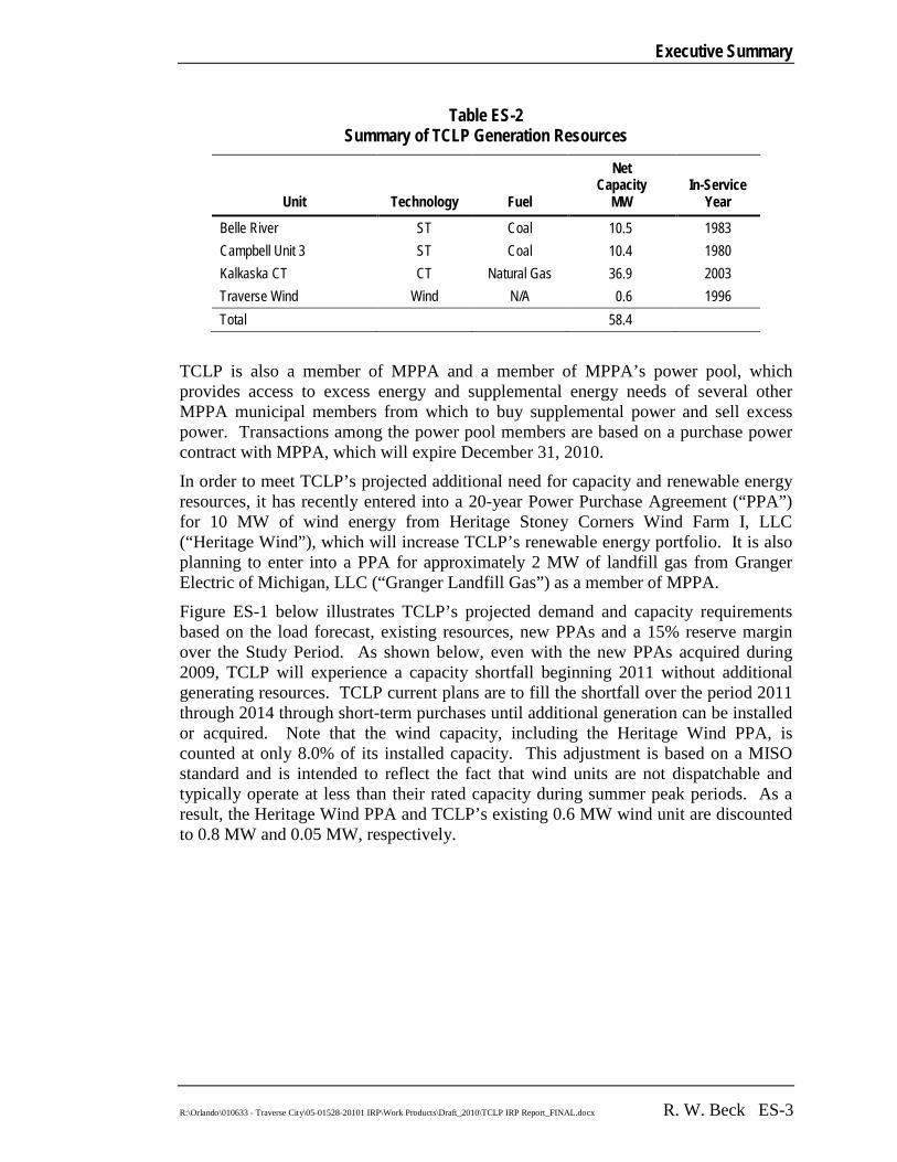
Executive Summary
R:\Orlando\010633 - Traverse City\05-01528-20101 IRP\Work Products\Draft_2010\TCLP IRP Report_FINAL.docx R. W. Beck ES-3
Table ES-2 Summary of TCLP Generation Resources
Unit Technology Fuel
Net Capacity
MW In-Service
Year
Belle River ST Coal 10.5 1983 Campbell Unit 3 ST Coal 10.4 1980 Kalkaska CT CT Natural Gas 36.9 2003 Traverse Wind Wind N/A 0.6 1996 Total 58.4
TCLP is also a member of MPPA and a member of MPPA’s power pool, which provides access to excess energy and supplemental energy needs of several other MPPA municipal members from which to buy supplemental power and sell excess power. Transactions among the power pool members are based on a purchase power contract with MPPA, which will expire December 31, 2010.
In order to meet TCLP’s projected additional need for capacity and renewable energy resources, it has recently entered into a 20-year Power Purchase Agreement (“PPA”) for 10 MW of wind energy from Heritage Stoney Corners Wind Farm I, LLC (“Heritage Wind”), which will increase TCLP’s renewable energy portfolio. It is also planning to enter into a PPA for approximately 2 MW of landfill gas from Granger Electric of Michigan, LLC (“Granger Landfill Gas”) as a member of MPPA.
Figure ES-1 below illustrates TCLP’s projected demand and capacity requirements based on the load forecast, existing resources, new PPAs and a 15% reserve margin over the Study Period. As shown below, even with the new PPAs acquired during 2009, TCLP will experience a capacity shortfall beginning 2011 without additional generating resources. TCLP current plans are to fill the shortfall over the period 2011 through 2014 through short-term purchases until additional generation can be installed or acquired. Note that the wind capacity, including the Heritage Wind PPA, is counted at only 8.0% of its installed capacity. This adjustment is based on a MISO standard and is intended to reflect the fact that wind units are not dispatchable and typically operate at less than their rated capacity during summer peak periods. As a result, the Heritage Wind PPA and TCLP’s existing 0.6 MW wind unit are discounted to 0.8 MW and 0.05 MW, respectively.
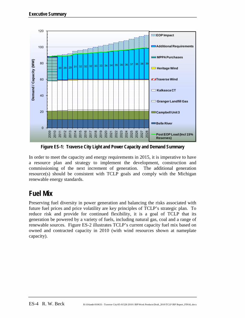
Executive Summary
ES-4 R. W. Beck R:\Orlando\010633 - Traverse City\05-01528-20101 IRP\Work Products\Draft_2010\TCLP IRP Report_FINAL.docx
Figure ES-1: Traverse City Light and Power Capacity and Demand Summary
In order to meet the capacity and energy requirements in 2015, it is imperative to have a resource plan and strategy to implement the development, construction and commissioning of the next increment of generation. The additional generation resource(s) should be consistent with TCLP goals and comply with the Michigan renewable energy standards.
Fuel Mix Preserving fuel diversity in power generation and balancing the risks associated with future fuel prices and price volatility are key principles of TCLP’s strategic plan. To reduce risk and provide for continued flexibility, it is a goal of TCLP that its generation be powered by a variety of fuels, including natural gas, coal and a range of renewable sources. Figure ES-2 illustrates TCLP’s current capacity fuel mix based on owned and contracted capacity in 2010 (with wind resources shown at nameplate capacity).
30 29 29 31 32 32 32 33 33 34 34 35 36 36 37 38 38 39
0
20
40
60
80
100
120
2009
2010
2011
2012
2013
2014
2015
2016
2017
2018
2019
2020
2021
2022
2023
2024
2025
2026
2027
2028
Dem
and
/ Cap
acity
(MW
)EOP Impact
Additional Requirements
MPPA Purchases
Heritage Wind
Traverse Wind
Kalkasca CT
Granger Landfill Gas
Campbell Unit 3
Belle River
Post EOP Load (Incl 15% Reserves)
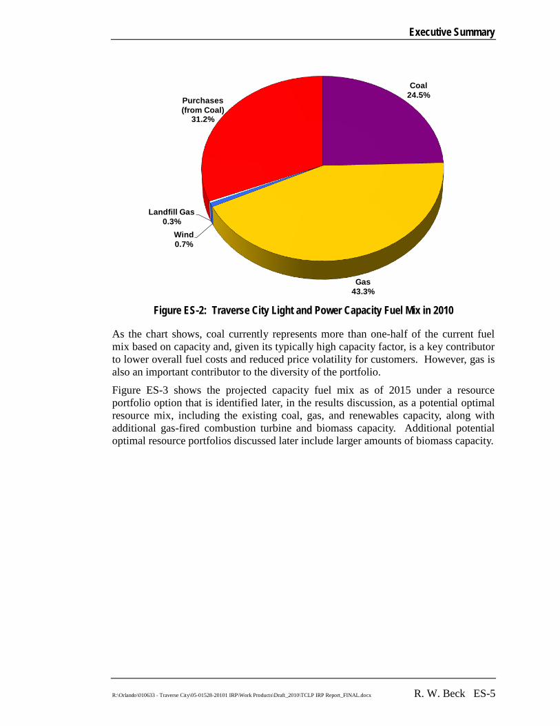
Executive Summary
R:\Orlando\010633 - Traverse City\05-01528-20101 IRP\Work Products\Draft_2010\TCLP IRP Report_FINAL.docx R. W. Beck ES-5
Figure ES-2: Traverse City Light and Power Capacity Fuel Mix in 2010
As the chart shows, coal currently represents more than one-half of the current fuel mix based on capacity and, given its typically high capacity factor, is a key contributor to lower overall fuel costs and reduced price volatility for customers. However, gas is also an important contributor to the diversity of the portfolio.
Figure ES-3 shows the projected capacity fuel mix as of 2015 under a resource portfolio option that is identified later, in the results discussion, as a potential optimal resource mix, including the existing coal, gas, and renewables capacity, along with additional gas-fired combustion turbine and biomass capacity. Additional potential optimal resource portfolios discussed later include larger amounts of biomass capacity.
Coal24.5%
Gas43.3%
Wind0.7%
Landfill Gas0.3%
Purchases(from Coal)
31.2%
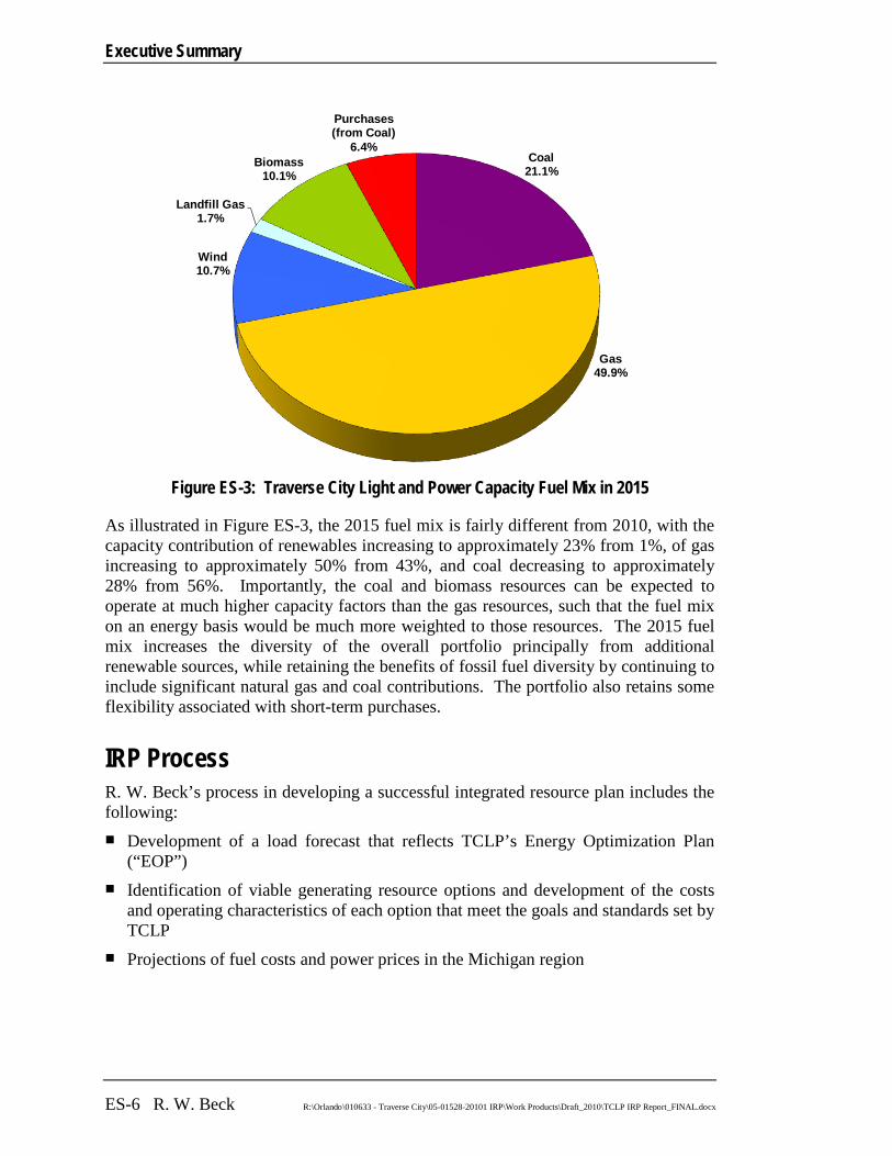
Executive Summary
ES-6 R. W. Beck R:\Orlando\010633 - Traverse City\05-01528-20101 IRP\Work Products\Draft_2010\TCLP IRP Report_FINAL.docx
Figure ES-3: Traverse City Light and Power Capacity Fuel Mix in 2015
As illustrated in Figure ES-3, the 2015 fuel mix is fairly different from 2010, with the capacity contribution of renewables increasing to approximately 23% from 1%, of gas increasing to approximately 50% from 43%, and coal decreasing to approximately 28% from 56%. Importantly, the coal and biomass resources can be expected to operate at much higher capacity factors than the gas resources, such that the fuel mix on an energy basis would be much more weighted to those resources. The 2015 fuel mix increases the diversity of the overall portfolio principally from additional renewable sources, while retaining the benefits of fossil fuel diversity by continuing to include significant natural gas and coal contributions. The portfolio also retains some flexibility associated with short-term purchases.
IRP Process R. W. Beck’s process in developing a successful integrated resource plan includes the following: Development of a load forecast that reflects TCLP’s Energy Optimization Plan
(“EOP”) Identification of viable generating resource options and development of the costs
and operating characteristics of each option that meet the goals and standards set by TCLP
Projections of fuel costs and power prices in the Michigan region
Coal21.1%
Gas49.9%
Wind10.7%
Landfill Gas1.7%
Biomass10.1%
Purchases(from Coal)
6.4%

Executive Summary
R:\Orlando\010633 - Traverse City\05-01528-20101 IRP\Work Products\Draft_2010\TCLP IRP Report_FINAL.docx R. W. Beck ES-7
Busbar1
Development of the optimal resource plan(s) that take into account costs and risks of all alternatives and combinations of alternatives
screening analyses of the generation options
Prior to performing the resource expansion optimization analysis, all generating resource alternatives evaluated for the IRP Study were assessed for their levelized cost (or average present value costs) over a consistent study period and operation relative to all other alternatives, a process frequently referred to as a busbar screening analysis.
Following the busbar screening analyses, the generating resource alternatives that were identified as reasonable candidates for further evaluation were combined in a resource expansion optimization model to identify an optimum resource expansion plan. The model used by R. W. Beck incorporates an algorithm that couples a rigorous dynamic programming optimization process with a stochastic2
Economic and financing assumptions, load forecast, fuel prices, emission allowance prices, generating resource characteristics and costs, and other general assumptions used to perform the generation expansion analysis are set forth in Section 2 of the Report and are summarized under the section entitled ‘Principal Considerations and Assumptions’ near the end of the Executive Summary.
representation of uncertain future conditions for load, fuel prices, carbon dioxide (“CO2”) prices, and power prices. The model thus produces a least-cost resource plan (at a given risk tolerance) by simulating the real option cost and value of resource expansion decision-making that occurs in actual utility practice.
Busbar Screening Analysis Results Generating resources are compared on a total average present value dollars per MWh basis over a range of capacity factors considered reasonable for the type of resource being evaluated. When a generating resource alternative is found to be lower cost than all, or many, other alternatives in a particular class of resources, the alternative would be retained for further investigation. Experience demonstrates that alternatives that possess the lowest average total production cost within a given operating range (capacity factor) using a busbar screening approach will likely also be identified as the principal alternatives selected through a more rigorous dynamic optimization analysis. The detailed results of the busbar screening analysis are set forth in Section 3 of this Report.
Figure ES-4 below provides a summary of the present value average costs, in 2008 dollars, over the period 2011 through 2028 of the resources included in the busbar screening analysis over a range of capacity factors.
1 The busbar screening analyses only include capital and operating costs of each resource alternative, but do not include the cost of transmission. The cost of transmission was assumed to be generally comparable for the evaluated resource alternatives. 2 Stochastic projections reflect the uncertainty and volatility in forecasting variables such as fuel costs and electric loads. A stochastic projection is usually captured by forecasting future values based on past economic behavior and numerous future outcomes. The resulting stochastic projection provides a range of potential values instead of one forecasted value.
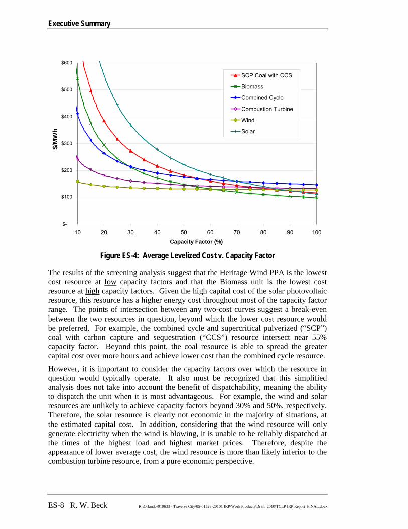
Executive Summary
ES-8 R. W. Beck R:\Orlando\010633 - Traverse City\05-01528-20101 IRP\Work Products\Draft_2010\TCLP IRP Report_FINAL.docx
Figure ES-4: Average Levelized Cost v. Capacity Factor
The results of the screening analysis suggest that the Heritage Wind PPA is the lowest cost resource at low capacity factors and that the Biomass unit is the lowest cost resource at high
However, it is important to consider the capacity factors over which the resource in question would typically operate. It also must be recognized that this simplified analysis does not take into account the benefit of dispatchability, meaning the ability to dispatch the unit when it is most advantageous. For example, the wind and solar resources are unlikely to achieve capacity factors beyond 30% and 50%, respectively. Therefore, the solar resource is clearly not economic in the majority of situations, at the estimated capital cost. In addition, considering that the wind resource will only generate electricity when the wind is blowing, it is unable to be reliably dispatched at the times of the highest load and highest market prices. Therefore, despite the appearance of lower average cost, the wind resource is more than likely inferior to the combustion turbine resource, from a pure economic perspective.
capacity factors. Given the high capital cost of the solar photovoltaic resource, this resource has a higher energy cost throughout most of the capacity factor range. The points of intersection between any two-cost curves suggest a break-even between the two resources in question, beyond which the lower cost resource would be preferred. For example, the combined cycle and supercritical pulverized (“SCP”) coal with carbon capture and sequestration (“CCS”) resource intersect near 55% capacity factor. Beyond this point, the coal resource is able to spread the greater capital cost over more hours and achieve lower cost than the combined cycle resource.
$-
$100
$200
$300
$400
$500
$600
10 20 30 40 50 60 70 80 90 100Capacity Factor (%)
$/M
Wh
SCP Coal with CCS
Biomass
Combined Cycle
Combustion Turbine
Wind
Solar
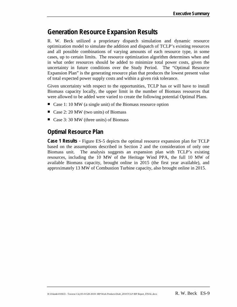
Executive Summary
R:\Orlando\010633 - Traverse City\05-01528-20101 IRP\Work Products\Draft_2010\TCLP IRP Report_FINAL.docx R. W. Beck ES-9
Generation Resource Expansion Results R. W. Beck utilized a proprietary dispatch simulation and dynamic resource optimization model to simulate the addition and dispatch of TCLP’s existing resources and all possible combinations of varying amounts of each resource type, in some cases, up to certain limits. The resource optimization algorithm determines when and in what order resources should be added to minimize total power costs, given the uncertainty in future conditions over the Study Period. The “Optimal Resource Expansion Plan” is the generating resource plan that produces the lowest present value of total expected power supply costs and within a given risk tolerance.
Given uncertainty with respect to the opportunities, TCLP has or will have to install Biomass capacity locally, the upper limit in the number of Biomass resources that were allowed to be added were varied to create the following potential Optimal Plans. Case 1: 10 MW (a single unit) of the Biomass resource option Case 2: 20 MW (two units) of Biomass Case 3: 30 MW (three units) of Biomass
Optimal Resource Plan Case 1 Results - Figure ES-5 depicts the optimal resource expansion plan for TCLP based on the assumptions described in Section 2 and the consideration of only one Biomass unit. The analysis suggests an expansion plan with TCLP’s existing resources, including the 10 MW of the Heritage Wind PPA, the full 10 MW of available Biomass capacity, brought online in 2015 (the first year available), and approximately 13 MW of Combustion Turbine capacity, also brought online in 2015.

Executive Summary
ES-10 R. W. Beck R:\Orlando\010633 - Traverse City\05-01528-20101 IRP\Work Products\Draft_2010\TCLP IRP Report_FINAL.docx
Figure ES-5: Optimal Plan – Case 1
Figure ES-6 below depicts the range of projected annual average power costs under the Case 1 Optimal Plan. The lines shown include the expected value, or mean, across the draws and the 5th and 95th percentiles, encompassing 90 percent of the potential power costs. In the upper left corner of the graph is shown the levelized power costs over the Study Period and the standard deviation, across the draws.
Figure ES-6: Range of Power Supply Costs – Case 1
0
20
40
60
80
100
120
2010
2011
2012
2013
2014
2015
2016
2017
2018
2019
2020
2021
2022
2023
2024
2025
2026
2027
2028
Meg
awat
ts
Market Purchases
New Solar
Heritage Wind
Combustion Turbine
Combined Cycle
SCP Coal wCCS
Granger Landfill Gas
Existing Wind
Kalkaska CT
TCLP Biomass
Campbell 3
Belle River
Peak Demand
Capacity Requirements
$-
$20
$40
$60
$80
$100
$120
$140
$160
$180
$/M
Wh
Expected Value 5th Percentile 95th Percentile
Levelized Average Cost: 99.97/MWhStandard Deviation: 10.93/MWh
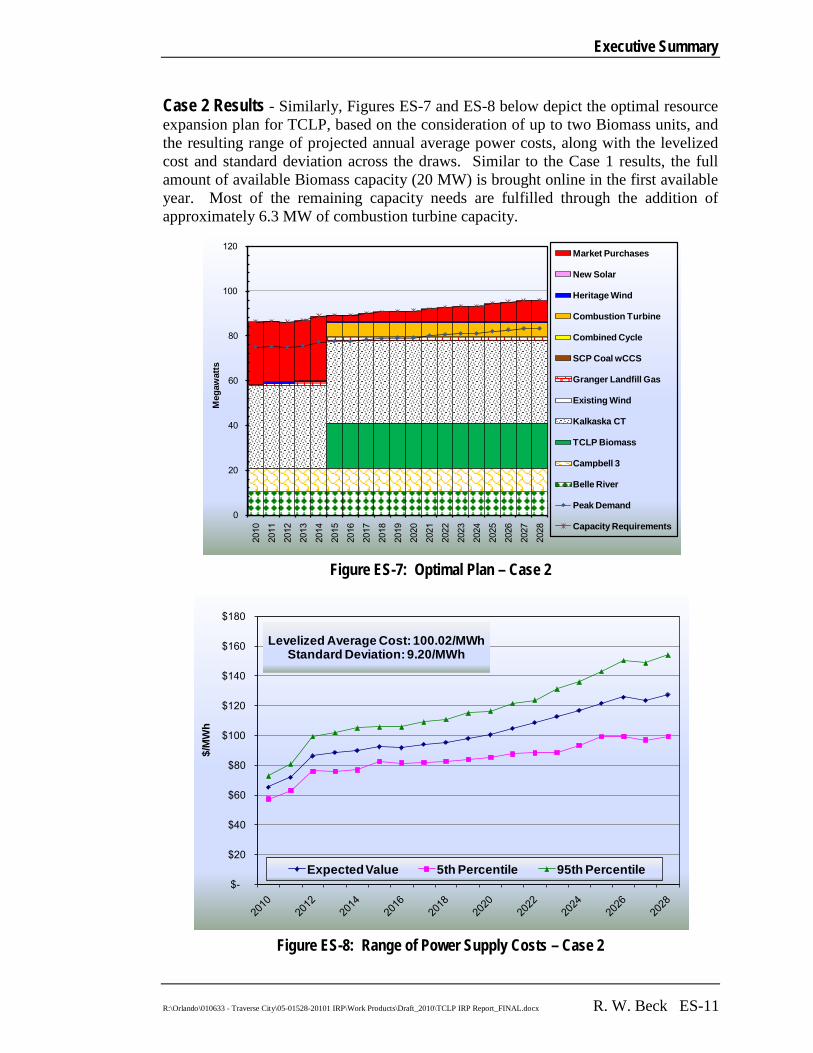
Executive Summary
R:\Orlando\010633 - Traverse City\05-01528-20101 IRP\Work Products\Draft_2010\TCLP IRP Report_FINAL.docx R. W. Beck ES-11
Case 2 Results - Similarly, Figures ES-7 and ES-8 below depict the optimal resource expansion plan for TCLP, based on the consideration of up to two Biomass units, and the resulting range of projected annual average power costs, along with the levelized cost and standard deviation across the draws. Similar to the Case 1 results, the full amount of available Biomass capacity (20 MW) is brought online in the first available year. Most of the remaining capacity needs are fulfilled through the addition of approximately 6.3 MW of combustion turbine capacity.
Figure ES-7: Optimal Plan – Case 2
Figure ES-8: Range of Power Supply Costs – Case 2
0
20
40
60
80
100
120 20
10
2011
2012
2013
2014
2015
2016
2017
2018
2019
2020
2021
2022
2023
2024
2025
2026
2027
2028
Meg
awat
ts
Market Purchases
New Solar
Heritage Wind
Combustion Turbine
Combined Cycle
SCP Coal wCCS
Granger Landfill Gas
Existing Wind
Kalkaska CT
TCLP Biomass
Campbell 3
Belle River
Peak Demand
Capacity Requirements
$-
$20
$40
$60
$80
$100
$120
$140
$160
$180
$/M
Wh
Expected Value 5th Percentile 95th Percentile
Levelized Average Cost: 100.02/MWhStandard Deviation: 9.20/MWh
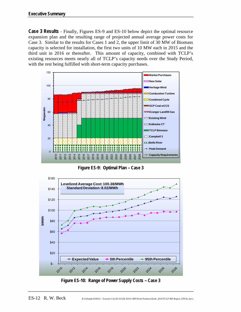
Executive Summary
ES-12 R. W. Beck R:\Orlando\010633 - Traverse City\05-01528-20101 IRP\Work Products\Draft_2010\TCLP IRP Report_FINAL.docx
Case 3 Results - Finally, Figures ES-9 and ES-10 below depict the optimal resource expansion plan and the resulting range of projected annual average power costs for Case 3. Similar to the results for Cases 1 and 2, the upper limit of 30 MW of Biomass capacity is selected for installation, the first two units of 10 MW each in 2015 and the third unit in 2016 or thereafter. This amount of capacity, combined with TCLP’s existing resources meets nearly all of TCLP’s capacity needs over the Study Period, with the rest being fulfilled with short-term capacity purchases.
Figure ES-9: Optimal Plan – Case 3
Figure ES-10: Range of Power Supply Costs – Case 3
0
20
40
60
80
100
120
2010
2011
2012
2013
2014
2015
2016
2017
2018
2019
2020
2021
2022
2023
2024
2025
2026
2027
2028
Meg
awat
ts
Market Purchases
New Solar
Heritage Wind
Combustion Turbine
Combined Cycle
SCP Coal wCCS
Granger Landfill Gas
Existing Wind
Kalkaska CT
TCLP Biomass
Campbell 3
Belle River
Peak Demand
Capacity Requirements
$-
$20
$40
$60
$80
$100
$120
$140
$160
$/M
Wh
Expected Value 5th Percentile 95th Percentile
Levelized Average Cost: 100.38/MWhStandard Deviation: 8.02/MWh

Executive Summary
R:\Orlando\010633 - Traverse City\05-01528-20101 IRP\Work Products\Draft_2010\TCLP IRP Report_FINAL.docx R. W. Beck ES-13
Sensitivity of Results to Natural Gas Prices In order to assess the sensitivity of the Optimal Plans to higher and lower natural gas prices, Cases 1 through 3 (again corresponding to varying levels of maximum allowed Biomass capacity) were re-simulated with higher and lower natural gas prices, set to the 70th and 30th percentiles, respectively. The resulting gas prices correspond to levels at which gas prices are only 30% likely to be higher or lower, respectively. Under the High Gas Prices sensitivity case, gas prices are on average approximately 27% higher than the expected gas prices. Under the Low Gas Prices sensitivity case, gas prices are on average approximately 21% lower than the expected prices.
The results of this scenario showed that the Optimal Plans in each case were essentially unaffected by the High Gas Prices sensitivity. This is primarily because the Optimal Plans already resulted in essentially the maximum amount of Biomass capacity possible being selected. The Combustion Turbine capacity selected in Cases 1 and 2 were also unaffected, as the market is similarly influenced by natural gas prices as the operating costs of this technology. However, the resulting market prices are still not high enough to warrant the higher capital costs of building the SCP Coal with CCS resource or additional renewable resources.
The Low Gas Prices sensitivity, on the other hand, resulted in Optimal Plans reflecting significant delays in the build-out of Biomass capacity. However, the ultimate amount of Biomass capacity that was reflected in the Optimal Plan was the same. Figure ES-11 provides an example, using the results of Case 2, which corresponds to a maximum allowed Biomass capacity of 20 MW. As compared to the results under expected gas prices, shown in Figure ES-7, the Optimal Plan under this sensitivity reflects only 10 MW of Biomass capacity added in 2015, with the remaining allowed 10 MW not built until 2026. The 6.3 MW of Combustion Turbine capacity is also added in 2015, as in the expected case. The Low Gas Prices sensitivity also reflects the market being relied upon for a greater share of capacity and energy needs.

Executive Summary
ES-14 R. W. Beck R:\Orlando\010633 - Traverse City\05-01528-20101 IRP\Work Products\Draft_2010\TCLP IRP Report_FINAL.docx
Figure ES-11: Optimal Plan – Case 2 (Low Gas Prices Sensitivity)
Costs versus Risks Figure ES-12 below provides a comparison of the three alternative Optimal Expansion Plans versus the Base Plan in the form of an X-Y chart, which combines both the levelized power cost over 2011-2028 for each plan and its standard deviation. The relative position of each plan along the X- and Y-axes corresponds to a trade-off between a preference for lower expected costs and a preference for projected costs of greater certainty (i.e., lower standard deviation), with points closer to the origin being overall more preferred. It is up to the utility planner to determine the acceptable trade-off between resource plans of lower cost versus those of lower uncertainty.
0
20
40
60
80
100
120
2010
2011
2012
2013
2014
2015
2016
2017
2018
2019
2020
2021
2022
2023
2024
2025
2026
2027
2028
Meg
awat
tsMarket Purchases
New Solar
Heritage Wind
Combustion Turbine
Combined Cycle
SCP Coal wCCS
Granger Landfill Gas
Existing Wind
Kalkaska CT
TCLP Biomass
Campbell 3
Belle River
Peak Demand
Capacity Requirements

Executive Summary
R:\Orlando\010633 - Traverse City\05-01528-20101 IRP\Work Products\Draft_2010\TCLP IRP Report_FINAL.docx R. W. Beck ES-15
Figure ES-12: Power Supply Costs Comparison
The results reflect that the Optimal Plans result in lower average levelized cost than the Existing Resources, and that they also successively lower the standard deviation of levelized power costs across the draws. The Optimal Plans add a significant amount of Biomass capacity, which both lowers the average levelized cost and significantly lowers the variability in levelized cost, which is evident in the lower standard deviation. This is most likely driven from the fact that the Biomass resource utilizes fuel that is subject to less volatility than gas-fired resources, based on the assumptions relied on herein, which also influence market prices more so than other fuel types.
The overall results discussed above suggest that, given the resource options that have been considered and the assumptions discussed in Section 2, TCLP is projected to achieve lower cost and greater certainty of cost with as much as 20-30 MW of Biomass capacity to be brought online over 2015-2026. These units are intended to operate at high capacity factors, and indeed must be to support steam or hot water sales to which they would be tied. Given that amount of capacity and TCLP’s other resources, it is estimated that as much as 40% of the energy generated by this amount of Biomass capacity would be surplus to be sold into the wholesale market for the first several years of the Study Period. While the risks associated with this surplus energy are accounted for in the simulations that support the additions of Biomass capacity, TCLP should consider its tolerance for risk and perhaps limit its exposure somewhat. Accordingly, the Case 2 results, which consist of the additions of 20 MW of Biomass capacity and approximately 6.3 MW of Combustion Turbine capacity appear most reasonable and representative of balancing TCLP’s goal of lowest cost and minimizing risk. Given the results of the Low Gas Prices sensitivity, TCLP might consider
7.6
8.4
9.2
10.0
10.8
11.6
12.4
99.5 100.0 100.5 101.0 101.5 102.0 102.5 103.0 103.5
Stan
dard
Dev
iatio
n
Levelized Cost ($/MWh)
Existing Resources Optimal Plan - Case 1
Optimal Plan - Case 2 Optimal Plan - Case 3

Executive Summary
ES-16 R. W. Beck R:\Orlando\010633 - Traverse City\05-01528-20101 IRP\Work Products\Draft_2010\TCLP IRP Report_FINAL.docx
building a smaller amount of Biomass capacity in the 2015 timeframe and building additional capacity somewhat later. This would afford TCLP some flexibility in the event that the relatively low natural gas prices that are evident today appear likely to be sustained in the long-term.
REP Results Figure ES-13 below provides a graphical representation of the projected amount of renewable generation in TCLP’s portfolio as compared to the REP goal outlined in Michigan Public Act 295. The chart shows that the Existing resources, with the Heritage PPA are projected to be well above the state requirements through 2014 and exactly meet the current State REP Goal for 2015 and beyond. The additions of significant amounts of Biomass capacity reflected in the Optimal Plans result in renewable generation that far exceed the State REP requirements, as well as TCLP’s RPS Goal, over the Study Period.
The State REP Goal shown below is intended to represent how that legislation will be interpreted for purposes of tracking TCLP’s renewable requirements. The growth in the renewable percentage through 2015 is based directly on the percentages outlined in the legislation, while the percentages beyond 2015 are based on the amount of renewables required in 2015 applied to the forecasted energy requirements, net of the EOP, over the forecast horizon. This results in a slightly declining required share of renewable generation, as TCLP’s energy requirements are forecasted to grow by 0.9% per year over 2010-2028.
Figure ES-13: Renewable Generation v. Michigan REP Goal
0%
10%
20%
30%
40%
50%
60%
70%
2010
2011
2012
2013
2014
2015
2016
2017
2018
2019
2020
2021
2022
2023
2024
2025
2026
2027
2028
Existing Resources Optimal Plan - Case 1 Optimal Plan - Case 3
Optimal Plan - Case 2 TCLP RPS Goal State REP Requirement
Executive Summary
R:\Orlando\010633 - Traverse City\05-01528-20101 IRP\Work Products\Draft_2010\TCLP IRP Report_FINAL.docx R. W. Beck ES-17
Principal Considerations and Assumptions In the preparation of this report and the opinions, which follow, we have made certain assumptions with respect to conditions that may occur in the future. TCLP has also made certain assumptions with respect to its projections of future operations. We have used and relied upon certain information and assumptions provided by TCLP, as well as certain information and assumptions provided to TCLP by others. To the extent that actual future conditions differ from those assumed herein, the actual results will vary from those forecast. The principal considerations and assumptions made in preparing this report that were made by us or provided to us by TCLP or others are set forth in Section 2 of the Report and the key assumptions are summarized below.
The generation resource options considered in the IRP include the following: Supercritical pulverized coal-fired steam plant with CCS (SCP Coal with CCS) –
8.5 MW Combined cycle gas turbine (SOLAR3
Simple cycle combustion turbine (SOLAR Model T70-SC1) – 6.3 MW
Model T70-CC1 with combined heat and power ‘CHP’ operation) – 8.0 MW
Solar Photovoltaic (Solar PV) – 0.1 MW per year (total of 0.5 MW available) Wind Heritage PPA (based on Heritage PPA prices) – 10 MW Biomass (Gasification configuration with CHP operation) – 10 MW (as defined by
TCLP)
For the SCP Coal with CCS resource, it is assumed that TCLP would jointly participate with other municipal or investor-owned utilities in a larger-scale plant totaling 544 MW.
3 SOLAR – Solar Turbines Incorporated, a subsidiary of Caterpillar Inc., is one of the world’s leading manufacturers of industrial gas turbines, with more than 13,400 units and over 1.4 billion operating hours in 96 countries.
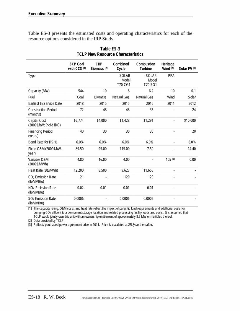
Executive Summary
ES-18 R. W. Beck R:\Orlando\010633 - Traverse City\05-01528-20101 IRP\Work Products\Draft_2010\TCLP IRP Report_FINAL.docx
Table ES-3 presents the estimated costs and operating characteristics for each of the resource options considered in the IRP Study.
Table ES-3 TCLP New Resource Characteristics
SCP Coal
with CCS [1] CHP
Biomass [2] Combined
Cycle Combustion
Turbine Heritage Wind [2] Solar PV [2]
Type SOLAR Model
T70-CG1
SOLAR Model
T70-SG1
PPA
Capacity (MW) 544 10 8 6.2 10 0.1 Fuel Coal Biomass Natural Gas Natural Gas Wind Solar Earliest In Service Date 2018 2015 2015 2015 2011 2012 Construction Period (months)
72 48 48 36 - 24
Capital Cost (2009$/kW; Incl’d IDC)
$6,774 $4,000 $1,428 $1,291 - $10,000
Financing Period (years)
40 30 30 30 - 20
Bond Rate for DS % 6.0% 6.0% 6.0% 6.0% - 6.0% Fixed O&M (2009$/kW-year)
89.50 95.00 115.00 7.50 - 14.40
Variable O&M (2009$/MWh)
4.80 16.00 4.00 - 105 [3] 0.00
Heat Rate (Btu/kWh) 12,200 8,500 9,623 11,655 - - CO2 Emission Rate (lb/MMBtu)
21 - 120 120 - -
NOX Emission Rate (lb/MMBtu)
0.02 0.01 0.01 0.01 - -
SO2 Emission Rate (lb/MMBtu)
0.0006 - 0.0006 0.0006 - -
[1] The capacity rating, O&M costs, and heat rate reflect the impact of parasitic load requirements and additional costs for pumping CO2 effluent to a permanent storage location and related processing facility loads and costs. It is assumed that TCLP would jointly own this unit with an ownership entitlement of approximately 8.5 MW or multiples thereof.
[2] Data provided by TCLP. [3] Reflects purchased power agreement price in 2011. Price is escalated at 2%/year thereafter.
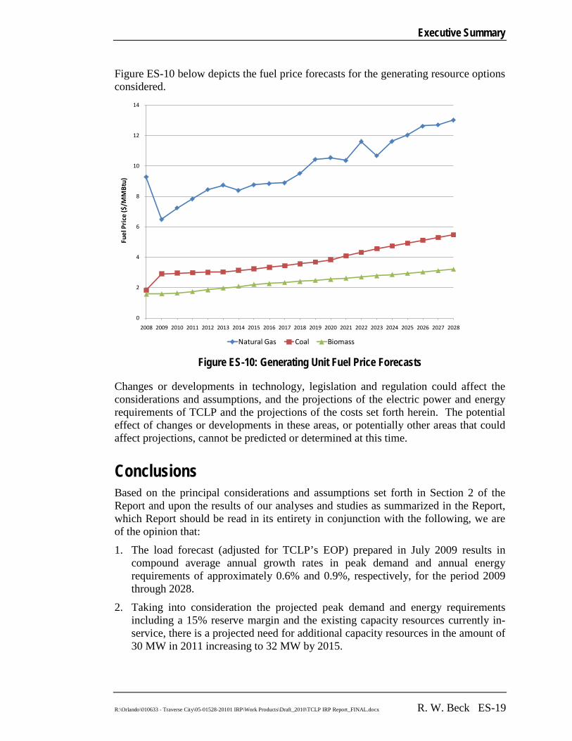
Executive Summary
R:\Orlando\010633 - Traverse City\05-01528-20101 IRP\Work Products\Draft_2010\TCLP IRP Report_FINAL.docx R. W. Beck ES-19
Figure ES-10 below depicts the fuel price forecasts for the generating resource options considered.
Figure ES-10: Generating Unit Fuel Price Forecasts
Changes or developments in technology, legislation and regulation could affect the considerations and assumptions, and the projections of the electric power and energy requirements of TCLP and the projections of the costs set forth herein. The potential effect of changes or developments in these areas, or potentially other areas that could affect projections, cannot be predicted or determined at this time.
Conclusions Based on the principal considerations and assumptions set forth in Section 2 of the Report and upon the results of our analyses and studies as summarized in the Report, which Report should be read in its entirety in conjunction with the following, we are of the opinion that:
1. The load forecast (adjusted for TCLP’s EOP) prepared in July 2009 results in compound average annual growth rates in peak demand and annual energy requirements of approximately 0.6% and 0.9%, respectively, for the period 2009 through 2028.
2. Taking into consideration the projected peak demand and energy requirements including a 15% reserve margin and the existing capacity resources currently in-service, there is a projected need for additional capacity resources in the amount of 30 MW in 2011 increasing to 32 MW by 2015.
0
2
4
6
8
10
12
14
2008 2009 2010 2011 2012 2013 2014 2015 2016 2017 2018 2019 2020 2021 2022 2023 2024 2025 2026 2027 2028
Fuel
Pri
ce ($
/MM
Btu
)
Natural Gas Coal Biomass
Executive Summary
ES-20 R. W. Beck R:\Orlando\010633 - Traverse City\05-01528-20101 IRP\Work Products\Draft_2010\TCLP IRP Report_FINAL.docx
3. The results of the busbar screening analysis indicate that the Biomass option is the lowest cost of the base-load resources (assuming an 85% capacity factor) over the period 2011 through 2028.
4. The results of the busbar screening analysis indicate that the Wind Resource is the lowest cost of the peaking resources (assuming a 25% capacity factor) over the period 2011 through 2028. However, the lack of dispatchability, combined with the typically lower generation during peak summer periods from wind resources, make the unit less economic than the Combustion Turbine resource option.
5. The Optimal Generating Resource Plan, which produces the lowest projected present value of total power supply costs and lowest risk over the Study Period, is an expansion plan with TCLP’s existing resources, including the 10 MW of the Heritage Wind PPA, and a build-out of Biomass generation totaling 20-30 MW over the Study Period and 0-13 MW of Combustion Turbine capacity, with larger amounts of Biomass capacity displacing the need for the CT capacity. The amounts of capacity from these two resource types that are most reasonable to be added depend on several factors, including (i) TCLP’s tolerance for the risk inherent in the potential for surplus energy generated from the larger amounts of Biomass capacity and (ii) the opportunities and the characteristics of the opportunities that TCLP is able to develop to install this CHP technology on its system.
6. Under the Higher Gas Price sensitivity case, the optimal expansion plans would be unchanged from the Optimal Plans under the Expected Case.
7. The Optimal Generating Resource Plan in Case 2 is projected to exceed the state REP requirements as well as TCLP’s REP goals over the Study Period. TCLP’s energy from renewable resources under the Optimal Generating Resource Plan Case 2 is projected to be 8.1% in 2011, 48% in 2015, 44% in 2020 and 43% in 2025.

Section 1 INTRODUCTION

R:\Orlando\010633 - Traverse City\05-01528-20101 IRP\Work Products\Draft_2010\TCLP IRP Report_FINAL.docx
Section 1 INTRODUCTION
1.1 Study Purpose As a result of the impending termination of a portion of its power supply arrangements, TCLP has initiated a power supply planning process to develop strategies to secure long-term, low-cost power, while meeting certain externally-imposed standards and internal goals regarding renewable resources. TCLP is faced with significant uncertainty in its power supply situation, including load growth uncertainty, fuel and power market price volatility, and uncertainty regarding possible environmental regulations. TCLP must develop a power supply plan that is low-cost, reliable, and capable of mitigating market price volatility, limits the impact of potential greenhouse gas legislation, and meets or exceeds current state and potential future federal renewable portfolio standards.
TCLP is entitled to capacity and energy from two coal-fired generation plants and a combustion turbine plant, through joint ownership arrangements with MPPA and nearby investor-owned utilities, and owns and operates a wind turbine in its service area. TCLP also purchases supplemental wholesale electricity to serve its retail load and sells surplus power through a power pool arrangement operated by MPPA. However, this power pool arrangement is scheduled to terminate at the end of 2010.
TCLP has retained R. W. Beck to conduct an IRP Study using a state-of-the-art stochastic4
Identify possible least-cost power supply plans (at a given risk tolerance) that will meet the future power supply needs of TCLP;
projections approach to:
Assess the potential impact that fuel and power market volatility may have on planning decisions; and
Assess how pending environmental legislation, chiefly greenhouse gas regulation, may affect power supply planning decisions.
The specific resource options and their costs and operating characteristics are set forth in Section 2.
The information contained in this report, regarding the existing facilities of TCLP, its current and planned operations, availability and cost of fuel supply, and environmental regulations, has been summarized from estimates, data, reports, permits, and records furnished by various sources. TCLP has also provided cost and operating 4 Stochastic projections reflect the uncertainty and volatility in forecasting variables such as fuel costs and electric loads. A stochastic projection is usually captured by forecasting future values based on past economic behavior and numerous future outcomes. The resulting stochastic projection provides a range of potential values instead of one forecasted value.
Section 1
1-2 R. W. Beck R:\Orlando\010633 - Traverse City\05-01528-20101 IRP\Work Products\Draft_2010\TCLP IRP Report_FINAL.docx
characteristics for certain future resource options as noted herein. While R. W. Beck believes such sources to be reliable, it has not verified the accuracy of any information furnished by or obtained from such sources and offers no assurances with respect thereto. To R. W. Beck’s knowledge, the summaries presented herein accurately reflect the information obtained from such sources. R. W. Beck has been advised that the information and advice are subject to change based on indeterminate future events that could include material changes in the cost and availability of fuel, in the regulation of environmental matters, in the estimated direct construction cost of electric generating facilities, in the ability of TCLP to finance major capital additions, in the management, ownership and regulation of TCLP and in other costs. Any such adverse changes could likely result in an increase in the projected costs of operating the TCLP electric system.
This study was performed under that certain agreement dated April 20, 2009 between TCLP and R. W. Beck (the “Agreement”). This report has been prepared for the use of TCLP for the specific purposes identified in this report. This report is solely for the information of and assistance to TCLP and should not be relied upon for any other purpose or by any other party unless authorized in writing by R. W. Beck in accordance with the Agreement.
The conclusions, observations, and recommendations contained herein attributed to R. W. Beck constitute the opinions of R. W. Beck. To the extent that statements, information, and opinions provided by TCLP or others have been used in the preparation of this report, R. W. Beck has relied upon the same to be accurate and provides no assurances or warranties to that effect. R. W. Beck makes no certification and gives no assurances except as explicitly set forth in this report. This report summarizes our work up to the date of this report; changed conditions, which occur or become known after such date could affect the results presented in the report to the extent of such changes.
1.2 Overview of TCLP TCLP is a municipally-owned entity of the City of Traverse City established in 1912 and governed by an Electric Utility Board. TCLP is responsible for providing power to approximately 11,000 customers within the City’s geographic limits and surrounding areas. In 2008, TCLP had a total annual load of approximately 343,000 MWh and summer peak demand of 64.9 MW.
TCLP has ownership shares in two coal-fired power plants—Belle River, operated by Detroit Edison, and Campbell 3, operated by Consumers Energy, an ownership share in a combustion turbine unit operated by MPPA, and owns and operates a wind turbine located in its service area. The combined dependable operating capacity of the TCLP generating facilities is approximately 58.4 MW. TCLP’s current generating resources are described in more detail in Table 1-1 below.

INTRODUCTION
R:\Orlando\010633 - Traverse City\05-01528-20101 IRP\Work Products\Draft_2010\TCLP IRP Report_FINAL.docx R. W. Beck 1-3
Table 1-1 Summary of TCLP Generation Resources
Unit Technology Fuel
Net Capacity
MW In-Service
Year
Belle River ST Coal 10.5 1983 Campbell Unit 3 ST Coal 10.4 1980 Kalkaska CT CT Natural Gas 36.9 2003 Traverse Wind Wind N/A 0.6 1996
TCLP is also a member of MPPA and a member of MPPA’s power pool, which provides access to excess energy and supplemental energy needs of several other MPPA municipal members from which to buy supplemental power and sell excess power. Transactions among the power pool members are based on a purchase power contract with MPPA, which will expire December 31, 2010. For purposes of this IRP Study, the earliest on-line date of potential resource additions, except future renewable resources is 2011, after the power pool arrangement has terminated.
1.3 Overview of the MISO East Market For purposes of the IRP Study, the market area in which TCLP resides is referred to as Midwest Independent Transmission System Operator (“MISO”) East, encompassing the lower peninsular Michigan, portions of Illinois, Indiana, Missouri, and Ohio. Figure 1-1 and Table 1-2, below, depict the assumed allocation of resources in the modeled MISO East region. The chart and table demonstrate that the region is currently dominated by coal capacity as a base-load resource, has very limited intermediate resources, and relatively small proportion of renewable capacity.
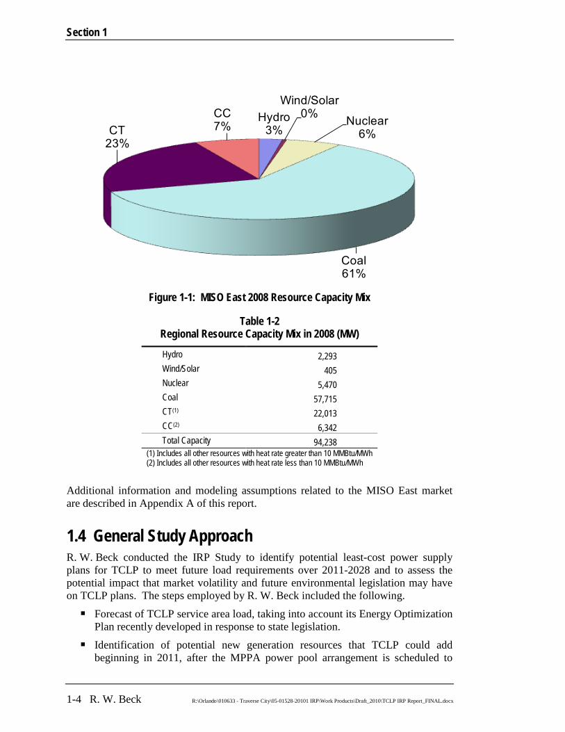
Section 1
1-4 R. W. Beck R:\Orlando\010633 - Traverse City\05-01528-20101 IRP\Work Products\Draft_2010\TCLP IRP Report_FINAL.docx
Figure 1-1: MISO East 2008 Resource Capacity Mix
Table 1-2 Regional Resource Capacity Mix in 2008 (MW)
Hydro 2,293 Wind/Solar 405 Nuclear 5,470 Coal 57,715 CT(1) 22,013 CC(2) 6,342 Total Capacity 94,238
(1) Includes all other resources with heat rate greater than 10 MMBtu/MWh (2) Includes all other resources with heat rate less than 10 MMBtu/MWh
Additional information and modeling assumptions related to the MISO East market are described in Appendix A of this report.
1.4 General Study Approach R. W. Beck conducted the IRP Study to identify potential least-cost power supply plans for TCLP to meet future load requirements over 2011-2028 and to assess the potential impact that market volatility and future environmental legislation may have on TCLP plans. The steps employed by R. W. Beck included the following.
Forecast of TCLP service area load, taking into account its Energy Optimization Plan recently developed in response to state legislation.
Identification of potential new generation resources that TCLP could add beginning in 2011, after the MPPA power pool arrangement is scheduled to
Hydro3%
Wind/Solar0% Nuclear
6%
Coal61%
CT23%
CC7%
INTRODUCTION
R:\Orlando\010633 - Traverse City\05-01528-20101 IRP\Work Products\Draft_2010\TCLP IRP Report_FINAL.docx R. W. Beck 1-5
terminate, and an assessment of capital cost, operating costs, and operating characteristics for these resources.
Forecast of fuel and emission prices for the MISO market area. Busbar screening cost analysis of potential generating resource options to rank
and identify the best resource alternatives for further consideration and study. Analysis and forecast of regional generation expansion and power prices for the
MISO East region using a stochastic simulation of fuel prices, power prices, CO2 allowance prices, hydro generation, and load for use in evaluating potential TCLP generation expansion plans.
Evaluation of potential least-cost power supply plans for TCLP using a dynamic optimization model and stochastic representation of loads, fuel prices, and CO2 allowance prices.
The study assumptions, including the results of the load forecast prepared by R. W. Beck in the Spring of 2009, are set forth in Section 2. The methodology and results of the busbar screening cost analysis are set forth in Section 3, and the methodology and results of the generation expansion analysis are set forth in Section 4. Detailed results of the power supply plan results are included in Appendix D. A list of acronyms used herein is set forth in Appendix E.


Section 2 STUDY ASSUMPTIONS


R:\Orlando\010633 - Traverse City\05-01528-20101 IRP\Work Products\Draft_2010\TCLP IRP Report_FINAL.docx
Section 2 STUDY ASSUMPTIONS
2.1 System Load Forecast R. W. Beck has prepared an econometric load forecast for TCLP through 2028, which reflects a “business-as-usual” growth trend, the results of which are shown in Table 2-1 below.
Table 2-1 TCLP Load Forecast - Prior to Energy Optimization Plan (EOP)
Fiscal Year Energy Calendar Year Peak Demand
(MWh) % Change (MW) % Change Load Factor
Historical 2006 347,380 3.0% 72.8 5.8% 54.5% 2007 347,639 0.1% 70.3 -3.4% 56.4% 2008 343,073 -1.3% 64.9 -7.6% 60.3%
Projected 2009 348,829 1.7% 74.8 15.2% 53.2% 2010 352,668 1.1% 75.5 0.9% 53.3% 2011 357,218 1.3% 76.3 1.1% 53.5% 2012 362,307 1.4% 77.0 0.9% 53.7% 2013 367,871 1.5% 78.2 1.6% 53.7% 2014 380,781 3.5%5 80.7 3.1% 53.9% 2015 386,941 1.6% 81.8 1.4% 54.0% 2016 393,402 1.7% 82.7 1.2% 54.3% 2017 399,986 1.7% 84.1 1.7% 54.3% 2018 406,849 1.7% 85.4 1.5% 54.4% 2019 413,898 1.7% 86.7 1.5% 54.5% 2020 421,220 1.8% 87.7 1.2% 54.8% 2021 428,645 1.8% 89.3 1.8% 54.8% 2022 436,336 1.8% 90.7 1.5% 54.9% 2023 444,201 1.8% 92.1 1.5% 55.1% 2024 452,322 1.8% 93.3 1.3% 55.4% 2025 460,621 1.8% 95.0 1.9% 55.4% 2026 469,174 1.9% 96.5 1.6% 55.5% 2027 477,811 1.8% 98.0 1.6% 55.6% 2028 486,708 1.9% 99.3 1.3% 55.9%
5 It has been assumed that TCLP will gain a significant number of customers from Consumers Energy beginning 2014.

Section 2
2-2 R. W. Beck R:\Orlando\010633 - Traverse City\05-01528-20101 IRP\Work Products\Draft_2010\TCLP IRP Report_FINAL.docx
Adjustments to the forecast have been developed to account for the implementation of an Energy Optimization Plan (“EOP”) as required under Michigan Public Act 295. Table 2-2 shows the annual incremental reductions in energy sales that are required under the legislation, in terms of the percentage of actual sales, averaged over the preceding three years that are to be reduced through TCLP’s energy efficiency programs. Table 2-3 below shows TCLP’s forecast after accounting for the impact of the EOP.
Table 2-2 Energy Optimization Plan Standard
Year Incremental Reduction
2009 0.30% 2010 0.50% 2011 0.75% 2012 and beyond 1.00%
Table 2-3 TCLP Load Forecast After EOP Impacts
Fiscal Year Energy Calendar Year Peak Demand
(MWH) % Change (MW) % Change Load Factor
2009 347,786 1.4% 74.6 14.9% 53.2% 2010 349,887 0.6% 74.9 0.4% 53.3% 2011 351,813 0.6% 75.1 0.3% 53.5% 2012 353,373 0.4% 75.1 -0.1% 53.7% 2013 355,363 0.6% 75.5 0.6% 53.7% 2014 364,649 2.6% 77.2 2.2% 53.9% 2015 367,082 0.7% 77.6 0.4% 54.0% 2016 369,711 0.7% 77.7 0.2% 54.3% 2017 372,354 0.7% 78.3 0.7% 54.3% 2018 375,211 0.8% 78.7 0.5% 54.5% 2019 378,189 0.8% 79.1 0.5% 54.6% 2020 381,371 0.8% 79.3 0.3% 54.9% 2021 384,585 0.8% 80.0 0.8% 54.9% 2022 387,993 0.9% 80.5 0.6% 55.1% 2023 391,499 0.9% 81.0 0.6% 55.2% 2024 395,186 0.9% 81.3 0.4% 55.5% 2025 398,971 1.0% 82.0 0.9% 55.5% 2026 402,929 1.0% 82.6 0.7% 55.7% 2027 406,889 1.0% 83.1 0.7% 55.9% 2028 411,023 1.0% 83.5 0.4% 56.2%
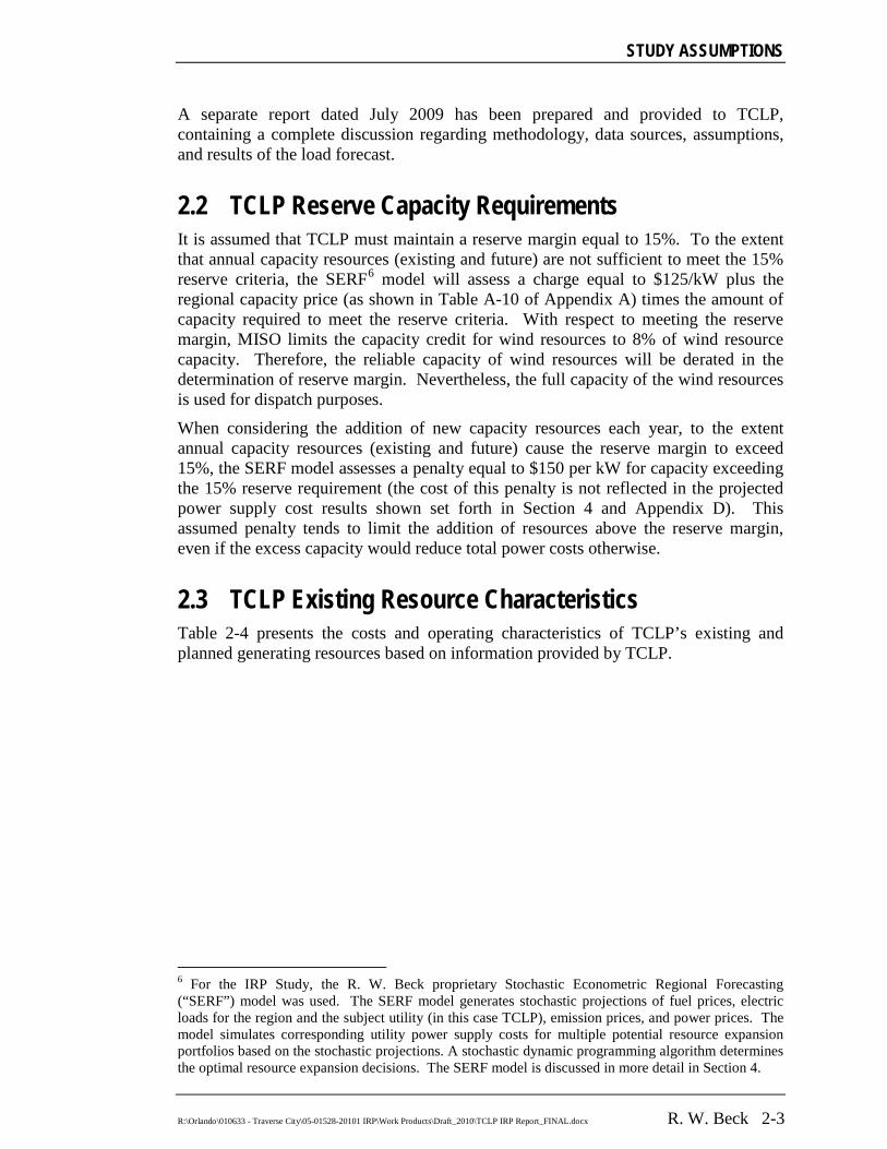
STUDY ASSUMPTIONS
R:\Orlando\010633 - Traverse City\05-01528-20101 IRP\Work Products\Draft_2010\TCLP IRP Report_FINAL.docx R. W. Beck 2-3
A separate report dated July 2009 has been prepared and provided to TCLP, containing a complete discussion regarding methodology, data sources, assumptions, and results of the load forecast.
2.2 TCLP Reserve Capacity Requirements It is assumed that TCLP must maintain a reserve margin equal to 15%. To the extent that annual capacity resources (existing and future) are not sufficient to meet the 15% reserve criteria, the SERF6
When considering the addition of new capacity resources each year, to the extent annual capacity resources (existing and future) cause the reserve margin to exceed 15%, the SERF model assesses a penalty equal to $150 per kW for capacity exceeding the 15% reserve requirement (the cost of this penalty is not reflected in the projected power supply cost results shown set forth in Section 4 and Appendix D). This assumed penalty tends to limit the addition of resources above the reserve margin, even if the excess capacity would reduce total power costs otherwise.
model will assess a charge equal to $125/kW plus the regional capacity price (as shown in Table A-10 of Appendix A) times the amount of capacity required to meet the reserve criteria. With respect to meeting the reserve margin, MISO limits the capacity credit for wind resources to 8% of wind resource capacity. Therefore, the reliable capacity of wind resources will be derated in the determination of reserve margin. Nevertheless, the full capacity of the wind resources is used for dispatch purposes.
2.3 TCLP Existing Resource Characteristics Table 2-4 presents the costs and operating characteristics of TCLP’s existing and planned generating resources based on information provided by TCLP.
6 For the IRP Study, the R. W. Beck proprietary Stochastic Econometric Regional Forecasting (“SERF”) model was used. The SERF model generates stochastic projections of fuel prices, electric loads for the region and the subject utility (in this case TCLP), emission prices, and power prices. The model simulates corresponding utility power supply costs for multiple potential resource expansion portfolios based on the stochastic projections. A stochastic dynamic programming algorithm determines the optimal resource expansion decisions. The SERF model is discussed in more detail in Section 4.

Section 2
2-4 R. W. Beck R:\Orlando\010633 - Traverse City\05-01528-20101 IRP\Work Products\Draft_2010\TCLP IRP Report_FINAL.docx
Table 2-4 TCLP Existing Resource Characteristics
Belle River Campbell
Unit 3 Kalkaska CT Wind
Turbine Granger
Landfill Gas
Fuel Coal Coal Natural Gas N/A Landfill Gas Prime Mover Steam Steam CT Wind CT TCLP Capacity (MW) 10.5 10.4 36.9 0.6 [1] [See Below] FOM Rate ($/kW-mo; $2008) 3.04 2.78 0.76 1.68 [See Below] VOM Rate ($/MWh; $2008) 2.16 1.95 5.00 4.03 [See Below] Average Heat Rate (Btu/kWh) 10,600 9,800 11,000 N/A [See Below] NOX Rate (lb/MMBtu) 0.070 0.070 0.070 N/A N/A SO2 Rate (lb/MMBtu) 0.100 0.100 0.100 N/A N/A CO2 Rate (lb/MMBtu) 210.0 210.0 120.0 N/A N/A Forced Outage Rate 4.0% 4.0% 0.0% N/A - [1] It is assumed that wind capacity is equivalent to only 8% of its nameplate for purposes of establishing resource adequacy
and reserve requirements.
TCLP is a participant in the planned Granger Landfill Gas project currently under development by MPPA. TCLP has entitlement shares that grow through time, as shown in Table 2-5 below. The energy cost ($/MWh) from the plant is also shown annually below.

STUDY ASSUMPTIONS
R:\Orlando\010633 - Traverse City\05-01528-20101 IRP\Work Products\Draft_2010\TCLP IRP Report_FINAL.docx R. W. Beck 2-5
Table 2-5 TCLP Granger Landfill Gas Entitlement
Year Capacity (MW) Energy Cost
($/MWh) 2009 0.00 77.68 2010 0.26 79.64 2011 0.78 81.63 2012 0.91 83.67 2013 1.43 85.77 2014 1.43 87.92 2015 1.69 90.12 2016 1.69 92.38 2017 1.69 94.69 2018 1.69 97.07 2019 1.69 99.50 2020 1.69 101.99 2021 1.69 104.55 2022 1.69 107.17 2023 1.69 109.85 2024 1.69 112.60 2025 1.69 115.42 2026 1.69 118.32 2027 1.69 121.28 2028 1.69 124.32
Figure 2-1 below illustrates TCLP’s projected demand and capacity requirements based on the load forecast and a 15% reserve margin over the Study Period. The chart reflects the addition of the Heritage Wind PPA, which provides TCLP with an entitlement to 10 MW of wind turbine capacity, beginning 2011. Note that both the existing wind unit and the Heritage Wind PPA are counted at only 8.0% of their installed capacity. This adjustment is based on a MISO standard and is intended to reflect the fact that wind units are not dispatchable and typically operate at less than their rated capacity during summer peak periods. As a result, the Heritage Wind PPA and TCLP’s existing 0.6 MW wind unit are discounted to 0.8 MW and 0.05 MW, respectively.

Section 2
2-6 R. W. Beck R:\Orlando\010633 - Traverse City\05-01528-20101 IRP\Work Products\Draft_2010\TCLP IRP Report_FINAL.docx
Figure 2-1: Traverse City Light and Power Capacity and Demand Summary
2.4 Existing Debt Service Table 2-6 below contains TCLP’s existing debt service schedule for its generation resources, as provided by TCLP staff. These costs are included in the projected power supply costs shown in Section 4.
Table 2-6 Traverse City Debt Service on MPPA Jointly-owned Units ($000)
Year Belle River Campbell 3 Kalkaska CT Total 2008 1,042 988 1,828 3,858 2009 1,054 806 1,825 3,685 2010 1,054 810 1,825 3,688 2011 1,054 811 1,827 3,692 2012 1,054 811 1,822 3,687 2013 1,054 796 1,822 3,672 2014 1,054 755 1,820 3,629 2015 1,054 715 1,822 3,590 2016 1,054 - 1,818 2,872 2017 1,054 - 1,819 2,872 2018 336 - 1,817 2,153 2019 - - 1,817 1,817 2020 - - 1,817 1,817
30 29 29 31 32 32 32 33 33 34 34 35 36 36 37 38 38 39
0
20
40
60
80
100
120
2009
2010
2011
2012
2013
2014
2015
2016
2017
2018
2019
2020
2021
2022
2023
2024
2025
2026
2027
2028
Dem
and
/ Cap
acity
(MW
)EOP Impact
Additional Requirements
MPPA Purchases
Heritage Wind
Traverse Wind
Kalkasca CT
Granger Landfill Gas
Campbell Unit 3
Belle River
Post EOP Load (Incl 15% Reserves)
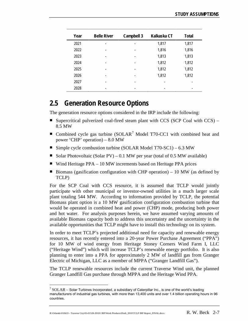
STUDY ASSUMPTIONS
R:\Orlando\010633 - Traverse City\05-01528-20101 IRP\Work Products\Draft_2010\TCLP IRP Report_FINAL.docx R. W. Beck 2-7
Year Belle River Campbell 3 Kalkaska CT Total 2021 - - 1,817 1,817 2022 - - 1,816 1,816 2023 - - 1,813 1,813 2024 - - 1,812 1,812 2025 - - 1,812 1,812 2026 - - 1,812 1,812 2027 - - - - 2028 - - - -
2.5 Generation Resource Options The generation resource options considered in the IRP include the following: Supercritical pulverized coal-fired steam plant with CCS (SCP Coal with CCS) –
8.5 MW Combined cycle gas turbine (SOLAR7
Simple cycle combustion turbine (SOLAR Model T70-SC1) – 6.3 MW
Model T70-CC1 with combined heat and power ‘CHP’ operation) – 8.0 MW
Solar Photovoltaic (Solar PV) – 0.1 MW per year (total of 0.5 MW available) Wind Heritage PPA – 10 MW increments based on Heritage PPA prices Biomass (gasification configuration with CHP operation) – 10 MW (as defined by
TCLP)
For the SCP Coal with CCS resource, it is assumed that TCLP would jointly participate with other municipal or investor-owned utilities in a much larger scale plant totaling 544 MW. According to information provided by TCLP, the potential Biomass plant option is a 10 MW gasification configuration combustion turbine that would be operated in combined heat and power (CHP) mode, producing both power and hot water. For analysis purposes herein, we have assumed varying amounts of available Biomass capacity both to address this uncertainty and the uncertainty in the available opportunities that TCLP might have to install this technology on its system.
In order to meet TCLP’s projected additional need for capacity and renewable energy resources, it has recently entered into a 20-year Power Purchase Agreement (“PPA”) for 10 MW of wind energy from Heritage Stoney Corners Wind Farm I, LLC (“Heritage Wind”) which will increase TCLP’s renewable energy portfolio. It is also planning to enter into a PPA for approximately 2 MW of landfill gas from Granger Electric of Michigan, LLC as a member of MPPA (“Granger Landfill Gas”).
The TCLP renewable resources include the current Traverse Wind unit, the planned Granger Landfill Gas purchase through MPPA and the Heritage Wind PPA.
7 SOLAR – Solar Turbines Incorporated, a subsidiary of Caterpillar Inc., is one of the world’s leading manufacturers of industrial gas turbines, with more than 13,400 units and over 1.4 billion operating hours in 96 countries.

Section 2
2-8 R. W. Beck R:\Orlando\010633 - Traverse City\05-01528-20101 IRP\Work Products\Draft_2010\TCLP IRP Report_FINAL.docx
Table 2-7 TCLP Renewable Resource Capacity (MW)
Traverse Wind
Granger Landfill Gas
Heritage Wind
2009 0.60 0.00 0.00 2010 0.60 0.26 0.00 2011 0.60 0.78 10.00 2012 0.60 0.91 10.00 2013 0.60 1.43 10.00 2014 0.60 1.43 10.00 2015 0.60 1.69 10.00 2016 0.60 1.69 10.00 2017 0.60 1.69 10.00 2018 0.60 1.69 10.00 2019 0.60 1.69 10.00 2020 0.60 1.69 10.00 2021 0.60 1.69 10.00 2022 0.60 1.69 10.00 2023 0.60 1.69 10.00 2024 0.60 1.69 10.00 2025 0.60 1.69 10.00 2026 0.60 1.69 10.00 2027 0.60 1.69 10.00 2028 0.60 1.69 10.00
The existing Traverse Wind unit is modeled using an assumed hourly generation pattern, developed by R. W. Beck, adjusted to a 15% capacity factor, based on the historical capacity factor reported by TCLP. The New Wind resource uses the same pattern, however adjusted to a 24% capacity factor, based on assumptions typically utilized in the MISO region. The Biomass unit is assumed to run at an 85% capacity factor, on a must-run basis. Similarly, the Granger Landfill Gas unit is assumed to run at 100% capacity factor since the arrangement with TCLP is an energy-only purchase.
Table 2-8 presents the associated costs, financing parameters, and operating characteristics for the renewable resources shown above, a solar resource, and potential non-renewable resource options. For the coal-fired resource, it is assumed that TCLP would jointly participate with other municipal or investor-owned utilities. The modeled size of TCLP’s entitlement to any of these resources is an outcome of the investment decision analysis embedded in the model, subject to the modeled sizing of “slices” of each resource as discussed in Section 4.

STUDY ASSUMPTIONS
R:\Orlando\010633 - Traverse City\05-01528-20101 IRP\Work Products\Draft_2010\TCLP IRP Report_FINAL.docx R. W. Beck 2-9
Table 2-8 TCLP New Resource Characteristics
SCP Coal
with CCS [1] CHP
Biomass [2] Combined
Cycle Combustion
Turbine Heritage Wind [2] Solar PV [2]
Type SOLAR Model T70-CG1
SOLAR Model T70-SG1
PPA
Capacity (MW) 544 10 8 6.2 10 0.1 Fuel Coal Biomass Natural Gas Natural Gas Wind Solar Earliest In Service Date
2018 2015 2015 2015 2011 2012
Construction Period (months)
72 48 48 36 - 24
Capital Cost (2009$/kW; Incl’d IDC)
$6,774 $4,000 $1,428 $1,291 -
$10,000
Financing Period (years)
40 30 30 30 - 20
Bond Rate for DS % 6.0% 6.0% 6.0% 6.0% - 6.0% Fixed O&M (2009$/kW-year)
89.50 95.00 115.00 7.50 - $14.40
Variable O&M (2009$/MWh)
4.80 16.00 4.00 - 105 [3] -
Heat Rate (Btu/kWh)
12,200 8,500 9,623 11,655 - -
CO2 Emission Rate (lb/MMBtu)
21 - 120 120 - -
NOX Emission Rate (lb/MMBtu)
0.02 0.01 0.01 0.01 - -
SO2 Emission Rate (lb/MMBtu)
0.0006 - 0.0006 0.0006 - -
[1] The capacity rating, O&M costs, and heat rate reflect the impact of parasitic load requirements and additional costs for pumping CO2 effluent to a permanent storage location and related processing facility loads and costs. It is assumed that TCLP would jointly own this unit with an ownership entitlement of approximately 8.5 MW or multiples thereof.
[2] Data provided by TCLP. [3] Reflects purchased power agreement price in 2011. Price is escalated at 2%/year thereafter.
2.6 Biomass Fuel Price Forecast To determine a price for biomass fuel, R. W. Beck developed a supply curve representation of the incremental costs of biomass fuel to the delivery point of a proposed generating station within the region surrounding Traverse City. The quantity of biomass feedstock used to develop the supply curve is based on publicly available sources of information in which the existing Biomass supply (dry tons/year) by county in Michigan was provided. The supply curve is based upon the costs of a mix of biomass feedstock (agricultural residues, forest residues, urban waste, switch grass and mill wastes) within 100 miles of Traverse City. While cheaper fuel sources exist beyond this radius, the supply radius was limited to reduce the effects of transportation on the supply curve. R. W. Beck’s research suggests that the current area demand for
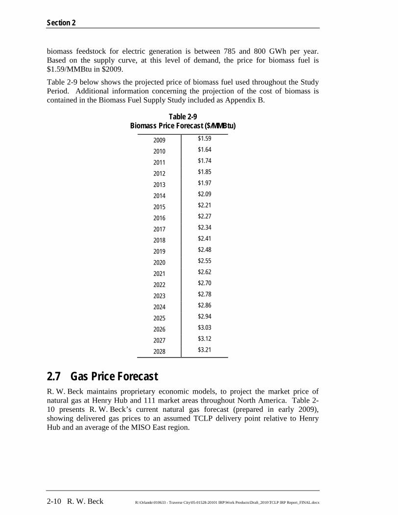
Section 2
2-10 R. W. Beck R:\Orlando\010633 - Traverse City\05-01528-20101 IRP\Work Products\Draft_2010\TCLP IRP Report_FINAL.docx
biomass feedstock for electric generation is between 785 and 800 GWh per year. Based on the supply curve, at this level of demand, the price for biomass fuel is $1.59/MMBtu in $2009.
Table 2-9 below shows the projected price of biomass fuel used throughout the Study Period. Additional information concerning the projection of the cost of biomass is contained in the Biomass Fuel Supply Study included as Appendix B.
Table 2-9 Biomass Price Forecast ($/MMBtu)
2009 $1.59
2010 $1.64
2011 $1.74
2012 $1.85
2013 $1.97
2014 $2.09
2015 $2.21
2016 $2.27
2017 $2.34
2018 $2.41
2019 $2.48
2020 $2.55
2021 $2.62
2022 $2.70
2023 $2.78
2024 $2.86
2025 $2.94
2026 $3.03
2027 $3.12
2028 $3.21
2.7 Gas Price Forecast R. W. Beck maintains proprietary economic models, to project the market price of natural gas at Henry Hub and 111 market areas throughout North America. Table 2-10 presents R. W. Beck’s current natural gas forecast (prepared in early 2009), showing delivered gas prices to an assumed TCLP delivery point relative to Henry Hub and an average of the MISO East region.
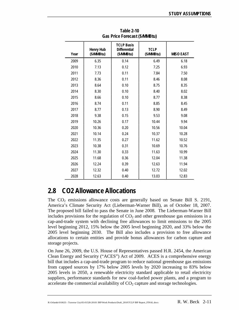
STUDY ASSUMPTIONS
R:\Orlando\010633 - Traverse City\05-01528-20101 IRP\Work Products\Draft_2010\TCLP IRP Report_FINAL.docx R. W. Beck 2-11
Table 2-10 Gas Price Forecast ($/MMBtu)
Year Henry Hub ($/MMBtu)
TCLP Basis Differential ($/MMBtu)
TCLP ($/MMBtu) MISO EAST
2009 6.35 0.14 6.49 6.18 2010 7.13 0.12 7.25 6.93 2011 7.73 0.11 7.84 7.50 2012 8.36 0.11 8.46 8.08 2013 8.64 0.10 8.75 8.35 2014 8.30 0.10 8.40 8.02 2015 8.66 0.10 8.77 8.38 2016 8.74 0.11 8.85 8.45 2017 8.77 0.13 8.90 8.49 2018 9.38 0.15 9.53 9.08 2019 10.26 0.17 10.44 9.94 2020 10.36 0.20 10.56 10.04 2021 10.14 0.24 10.37 10.28 2022 11.35 0.27 11.62 10.52 2023 10.38 0.31 10.69 10.76 2024 11.30 0.33 11.63 10.99 2025 11.68 0.36 12.04 11.38 2026 12.24 0.39 12.63 11.94 2027 12.32 0.40 12.72 12.02 2028 12.63 0.40 13.03 12.83
2.8 CO2 Allowance Allocations The CO2 emissions allowance costs are generally based on Senate Bill S. 2191, America’s Climate Security Act (Lieberman-Warner Bill), as of October 18, 2007. The proposed bill failed to pass the Senate in June 2008. The Lieberman-Warner Bill includes provisions for the regulation of CO2 and other greenhouse gas emissions in a cap-and-trade system with declining free allowances to limit emissions to the 2005 level beginning 2012, 15% below the 2005 level beginning 2020, and 33% below the 2005 level beginning 2030. The Bill also includes a provision to free allowance allocations to certain entities and provide bonus allowances for carbon capture and storage projects.
On June 26, 2009, the U.S. House of Representatives passed H.R. 2454, the American Clean Energy and Security (“ACES”) Act of 2009. ACES is a comprehensive energy bill that includes a cap-and-trade program to reduce national greenhouse gas emissions from capped sources by 17% below 2005 levels by 2020 increasing to 83% below 2005 levels in 2050, a renewable electricity standard applicable to retail electricity suppliers, performance standards for new coal-fueled power plants, and a program to accelerate the commercial availability of CO2 capture and storage technologies.

Section 2
2-12 R. W. Beck R:\Orlando\010633 - Traverse City\05-01528-20101 IRP\Work Products\Draft_2010\TCLP IRP Report_FINAL.docx
If ACES were to be enacted, fossil generating units would become subject to the cap-and-trade program, beginning in 2012. Under the program, each unit must possess emission allowances equal to its annual metric tons of greenhouse gases emitted. Except for merchant coal units and long-term contract generators as defined in the bill and for qualifying CO2 capture and sequestration projects at electric generating units, no allowances would be allocated to fossil generating units. Allowances would be allocated to electricity local distribution companies for a limited number of years subject to prohibitions related to actual CO2 emissions and use limitations prescribed by the bill. The renewable electricity standard set forth in ACES applies to retail electric suppliers with annual retail sales of at least four million MWh, which is well above the annual sales level of TCLP.
2.9 TCLP Renewable Generation Goals Without a federal RPS, adoption and enforcement of an RPS have primarily taken place at the state level. The State of Michigan has codified an RPS in Public Act 295, which establishes the requirement for utilities to develop Renewable Energy Plans (“REP”) with specific requirements pertaining to the amount of renewable generation, or credits, to be produced each year.
Table 2-11 shows the Michigan REP requirements that were in place at the time of the study and the RPS goals set forth by TCLP. The REP requirements shown below utilize the projected growth rates of TCLP’s system (net of its EOP) and assume that the amount of required renewable generation credits are held constant beginning 2015, per the state legislation and consistent with TCLP’s filed REP. Accordingly, the required percentage of renewable generation in any year will gradually decline, as a result of load growth. As the table shows, TCLP has more aggressive goals than the state.
Table 2-11 Summary of Michigan RPS Requirements
MI REP
Requirements TCLP Goal
2009 0.0% 0.0% 2010 0.0% 0.0% 2011 0.0% 0.0% 2012 2.0% 2.0% 2013 3.3% 3.3% 2014 5.0% 5.0% 2015 10.0% 10.0% 2016 9.9% 14.0% 2017 9.9% 18.0% 2018 9.8% 22.0% 2019 9.7% 26.0% 2020 9.6% 30.0% 2021 9.5% 30.0%

STUDY ASSUMPTIONS
R:\Orlando\010633 - Traverse City\05-01528-20101 IRP\Work Products\Draft_2010\TCLP IRP Report_FINAL.docx R. W. Beck 2-13
MI REP
Requirements TCLP Goal
2022 9.5% 30.0% 2023 9.4% 30.0% 2024 9.3% 30.0% 2025 9.2% 30.0% 2026 9.1% 30.0% 2027 9.0% 30.0% 2028 8.9% 30.0%
Figure 2-2 below depicts the projected energy from TCLP’s current renewable projects (including the Heritage Wind PPA) as compared to the Michigan RPS requirements. Note that the Michigan REP legislation requires that renewable generation, or renewable credits, equal to 10% of the prior year’s energy requirements must be utilized in 2015 to meet TCLP’s energy requirements. For each year beyond 2015, the currently required amount of renewable generation is constant.
Figure 2-2. TCLP RPS Requirements and Resources
0
5
10
15
20
25
30
35
40
45
2009 2010 2011 2012 2013 2014 2015 2016 2017 2018 2019 2020 2021 2022 2023 2024 2025 2026 2027 2028
Ren
ewab
le G
ener
atio
n (G
Wh)
Wind Landfill Gas State REP Requirement


Section 3 BUSBAR SCREENING ANALYSIS

R:\Orlando\010633 - Traverse City\05-01528-20101 IRP\Work Products\Draft_2010\TCLP IRP Report_FINAL.docx
Section 3 BUSBAR SCREENING ANALYSIS
Prior to performing the resource expansion optimization analysis, all generating resource alternatives evaluated for the IRP Study were assessed for their levelized cost (or average present value costs) over a consistent Study Period relative to all other alternatives, a process frequently referred to as a busbar screening analysis.
3.1 Methodology Generating resources are compared on a total average present value dollars per MWh basis at particular capacity factors considered reasonable for the type of resource being evaluated. When a generating resource alternative is found to be lower cost than all, or many, other alternatives in a particular class of resources, the alternative would be retained for further investigation. Experience demonstrates that alternatives that possess the lowest average total production cost within a given operating range (capacity factor) using a busbar screening approach will likely also be identified as the principal alternatives selected through a more rigorous dynamic optimization analysis. However, some higher cost resource options might still be retained for further consideration and analysis if the options that were found to be lower cost are known to be limited in the total number that can be installed or in the timing of their installation (e.g., carbon capture and sequestration resources are expected to be unavailable until 2018 at the earliest) or would be needed to meet renewable generation goals, both internal and government-mandated.
For resources for which the operating capacity factor under an economic dispatch in MISO would be unlikely to be attained, replacement power is assumed to be purchased from the MISO market to supplement the unit’s operation at a lower capacity factor. Similarly, for resources that are considered not fully dispatchable at their full capacity to meet peak demand, typically assumed to be in the summer (e.g., wind and solar capacity), backstand capacity is assumed to be purchased to supplement the resource capacity available.
The busbar screening analysis was performed using the following major assumptions. Resource capital costs, construction spending curve, O&M costs, and operating
characteristics as depicted in Section 2, Table 2-8. Assumed municipal cost of debt and discount rate as discussed in Section 2,
Table 2.8. Fuel and emissions price forecasts consistent with those presented in Section 2,
Table 2-8. Common installation year of 2012, financing and operating period of thirty
years, and common present-value discount year of 2009.
Section 3
3-2 R. W. Beck R:\Orlando\010633 - Traverse City\05-01528-20101 IRP\Work Products\Draft_2010\TCLP IRP Report_FINAL.docx
The costs of replacement power and backstand capacity are based on the power market simulation discussed in Appendix A and set forth on Tables A-9 and A-10.
The resulting average costs are compared separately for base-load/intermediate resources and peaking resources. Base-load/intermediate resources include a combined cycle plant, a super-critical pulverized (“SCP”) coal plant, both with and without carbon capture and sequestration (“CCS”), and a biomass plant. As discussed further below, the SCP coal option without CCS has been included for comparative purposes only, as this resource type was excluded from the generation expansion analysis discussed in Section 4. Peaking resources include a gas turbine, wind turbine, and a photovoltaic solar generator.
The capital and operating costs and financing assumptions are as discussed in Section 2.5. The base-load/intermediate resources assume an 85% capacity factor. The combined cycle resource would only be expected to operate at a 70% capacity factor, and the analysis reflects additional off-peak market energy to make up the difference between 70% and 85% capacity factors. The peaking resources assume a 25% capacity factor. The combustion turbine is assumed to operate at an 11% capacity factor, and the analysis reflects additional market energy to make up the difference between 11% and 25% capacity factors. In addition, as the wind and solar units are not dispatchable, the capacity of those resources have been derated to 8% and 47%, respectively, and the cost of market capacity to bring the units to full capacity is included and shown in the replacement energy category.
3.2 Results Figure 3-1 below provides a summary of the present value average costs assuming an 85% capacity factor, in 2009 dollars, over the period 2011 through 2028 of the base-load and intermediate resources included in the busbar screening analysis. As shown below, the projections indicate that the Biomass plant and the SCP Coal resource options are the lowest cost of the base-load resources. However, the current regulatory environment in the State of Michigan has made the development of coal-fired generation very difficult. Accordingly, in consultation with TCLP, R. W. Beck has only considered the coal option with CCS in the generation expansion analysis discussed in Section 4.

BUSBAR SCREENING ANALYSIS
R:\Orlando\010633 - Traverse City\05-01528-20101 IRP\Work Products\Draft_2010\TCLP IRP Report_FINAL.docx R. W. Beck 3-3
Figure 3-1: Average Present Value Cost of Base-load Resource Options
Figure 3-2 below provides a summary of the present value average costs assuming a 25% capacity factor over the period 2011 through 2028 of the peaking resources included in the busbar screening analysis. As shown below, the Combustion Turbine option is fairly similar in cost to the Heritage Wind resource. The Solar resource is the most expensive of this category and, based on the generation expansion analysis discussed in the next section, is not economic across the majority of scenarios included.
$150
$106
$126
$106
0
20
40
60
80
100
120
140
160
Combined Cycle SCP Coal SCP Coal with CCS Biomass
$/M
Wh
Environmental Non-Fuel O&M Replacement Energy Fuel Fixed Costs
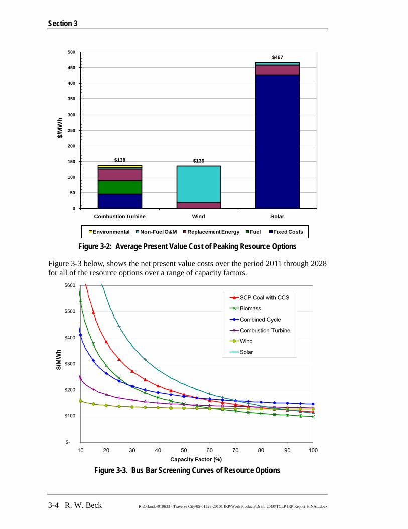
Section 3
3-4 R. W. Beck R:\Orlando\010633 - Traverse City\05-01528-20101 IRP\Work Products\Draft_2010\TCLP IRP Report_FINAL.docx
Figure 3-2: Average Present Value Cost of Peaking Resource Options
Figure 3-3 below, shows the net present value costs over the period 2011 through 2028 for all of the resource options over a range of capacity factors.
Figure 3-3. Bus Bar Screening Curves of Resource Options
$138 $136
$467
0
50
100
150
200
250
300
350
400
450
500
Combustion Turbine Wind Solar
$/M
Wh
Environmental Non-Fuel O&M Replacement Energy Fuel Fixed Costs
$-
$100
$200
$300
$400
$500
$600
10 20 30 40 50 60 70 80 90 100Capacity Factor (%)
$/M
Wh
SCP Coal with CCS
Biomass
Combined Cycle
Combustion Turbine
Wind
Solar

BUSBAR SCREENING ANALYSIS
R:\Orlando\010633 - Traverse City\05-01528-20101 IRP\Work Products\Draft_2010\TCLP IRP Report_FINAL.docx R. W. Beck 3-5
These results, combined with TCLP’s current power supply situation and its planned future renewable resource additions, were used to determine the most useful and appropriate amounts of each resource type to include in the generation resource optimization analysis discussed in the next section.


Section 4 GENERATION EXPANSION ANALYSIS

R:\Orlando\010633 - Traverse City\05-01528-20101 IRP\Work Products\Draft_2010\TCLP IRP Report_FINAL.docx
Section 4 GENERATION EXPANSION ANALYSIS
Following the busbar screening analyses, the generating resource alternatives that were identified as reasonable candidates for further evaluation were combined with the existing resources in a resource expansion optimization model to identify an optimal resource expansion plan. The model used by R. W. Beck incorporates an algorithm that couples a rigorous dynamic programming optimization process with a stochastic8
Economic and financing assumptions, load forecast, fuel prices, emission allowance prices, generating resource characteristics and costs, and other general assumptions used to perform the generation expansion analysis are consistent with the principal considerations and assumptions identified in Section 2 of this report.
representation of uncertain future conditions for load, fuel prices, CO2 prices, and power prices. The model thus produces a least-cost resource plan (at a given risk tolerance) by simulating the real option cost and value of resource expansion decision-making that occurs in actual utility practice.
4.1 Stochastic Econometric Regional Forecasting Model For this IRP Study, R. W. Beck has utilized a proprietary stochastic-dynamic resource optimization-planning model, referred to as the SERF model. The SERF model generates stochastic projections of fuel prices, electric loads for the region and the subject utility (in this case TCLP), emission prices, and power prices. The model simulates corresponding utility power supply costs for multiple potential resource expansion portfolios across all of the stochastic projections. A stochastic-dynamic programming algorithm determines the optimal resource expansion decisions given the future uncertainty in power costs. The general structure of the SERF model is depicted below in Figure 4-1.
SERF consists of three primary modules: Stochastic Market Module, which generates stochastic projections of fuel,
power prices, utility loads, and emission prices and simulates the build-out and commitment/dispatch of market resources;
Production Cost Module, which simulates a utility’s generating resource commitment and dispatch; and
Stochastic–Dynamic Optimization Module, which determines a utility’s optimal generation expansion plan given uncertain load, market, and commodity price conditions.
8 Stochastic projections reflect the uncertainty and volatility in forecasting variables such as fuel costs and electric loads. A stochastic projection is usually captured by forecasting future values based on past economic behavior and numerous future outcomes. The resulting stochastic projection provides a range of potential values instead of one forecasted value.

Section 4
4-2 R. W. Beck R:\Orlando\010633 - Traverse City\05-01528-20101 IRP\Work Products\Draft_2010\TCLP IRP Report_FINAL.docx
Figure 4-1: SERF Model Overview
A more detailed description of the SERF Model is included in Appendix C.
4.2 Market Simulation Results Examples of the stochastic forecasts of load, fuel prices, and power prices are depicted in the following figures. More comprehensive market results can be found in Section 3 of Appendix A. These results represent the random stochastic paths produced by the Stochastic Market Module using the expected (or average) values for load, fuel, and emission prices depicted in Section 2 of the report. In the figures, each colored line represents a separate random path, as described above, totaling 50 separate forecasts, with the heavy black lines representing the mean and the 5th and 95th percentiles of the random paths.
The cost of biomass fuel in each year is assumed to vary from the base case, or mean, forecast across the random stochastic paths in the same way as coal prices; therefore, the random paths of biomass fuel prices would look similar to those presented in Figure 4-4.
LoadForecast
LoadForecast
FuelPrice Forecast
FuelPrice Forecast
TransmissionSystem Analysis
TransmissionSystem Analysis
Existing Resource
Characteristics
Existing Resource
CharacteristicsNew Resource
OptionsNew Resource
Options
Develop Regional Load, Market and Fuel Price Scenarios (Draws)
Develop Regional Load, Market and Fuel Price Scenarios (Draws)
Simulation of Potential Power Supply PortfoliosUnder Scenarios (Draws) of Prices and Load
Simulation of Potential Power Supply PortfoliosUnder Scenarios (Draws) of Prices and Load
Identify Least-Cost / Risk Plan(s) and Develop Resource Selection RulesIdentify Least-Cost / Risk Plan(s) and Develop Resource Selection Rules
STOCHASTIC MARKET MODULE
PARAMETERS
PORTFOLIO DEVELOPMENT MODULE
PRODUCTION COST MODULE
STOCHASTIC-DYNAMIC OPTIMIZATION MODULE
Construct Portfolios ofPossible Resource Options
Construct Portfolios ofPossible Resource Options
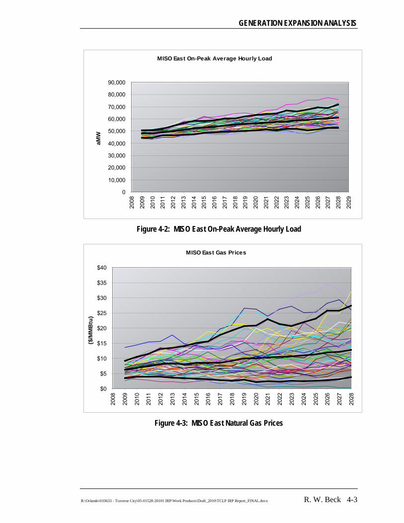
GENERATION EXPANSION ANALYSIS
R:\Orlando\010633 - Traverse City\05-01528-20101 IRP\Work Products\Draft_2010\TCLP IRP Report_FINAL.docx R. W. Beck 4-3
Figure 4-2: MISO East On-Peak Average Hourly Load
Figure 4-3: MISO East Natural Gas Prices
MISO East On-Peak Average Hourly Load
0
10,000
20,000
30,000
40,000
50,000
60,000
70,000
80,000
90,000
2008
2009
2010
2011
2012
2013
2014
2015
2016
2017
2018
2019
2020
2021
2022
2023
2024
2025
2026
2027
2028
2029
aMW
MISO East Gas Prices
$0
$5
$10
$15
$20
$25
$30
$35
$40
2008
2009
2010
2011
2012
2013
2014
2015
2016
2017
2018
2019
2020
2021
2022
2023
2024
2025
2026
2027
2028
($/M
MB
tu)
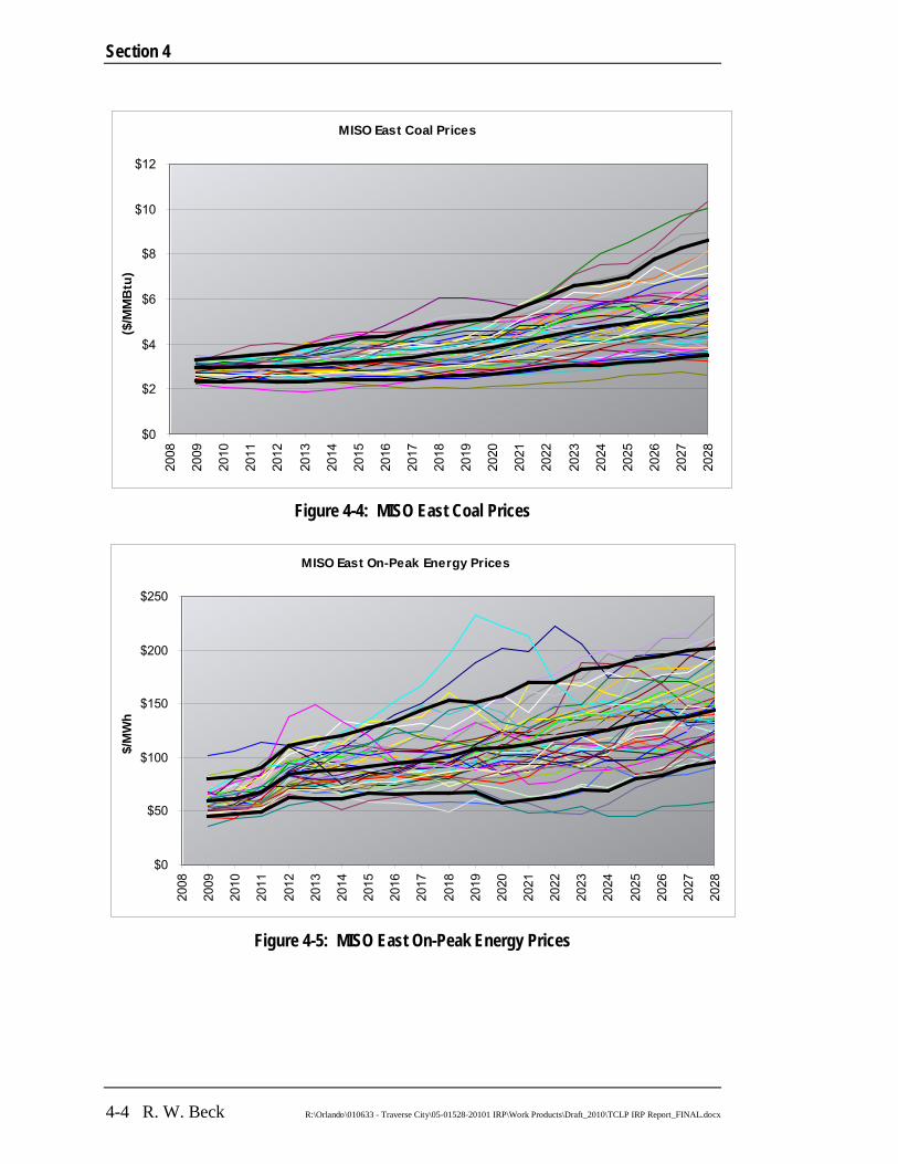
Section 4
4-4 R. W. Beck R:\Orlando\010633 - Traverse City\05-01528-20101 IRP\Work Products\Draft_2010\TCLP IRP Report_FINAL.docx
Figure 4-4: MISO East Coal Prices
Figure 4-5: MISO East On-Peak Energy Prices
MISO East Coal Prices
$0
$2
$4
$6
$8
$10
$1220
08
2009
2010
2011
2012
2013
2014
2015
2016
2017
2018
2019
2020
2021
2022
2023
2024
2025
2026
2027
2028
($/M
MB
tu)
MISO East On-Peak Energy Prices
$0
$50
$100
$150
$200
$250
2008
2009
2010
2011
2012
2013
2014
2015
2016
2017
2018
2019
2020
2021
2022
2023
2024
2025
2026
2027
2028
$/M
Wh
GENERATION EXPANSION ANALYSIS
R:\Orlando\010633 - Traverse City\05-01528-20101 IRP\Work Products\Draft_2010\TCLP IRP Report_FINAL.docx R. W. Beck 4-5
4.3 Generation Resource Expansion Plan Results In order to utilize SERF to study potential resource expansion plans, it is first necessary to specify the available resource options from which capacity additions can be made, including both their operating characteristics and size. In addition, any restrictions as to the timing of their addition must be specified.
The detailed assumptions related to other generating resource options to be considered by the SERF model are shown in Table 2-8 of Section 2. These options include the following: Supercritical pulverized coal-fired steam plant with CCS (SCP Coal with CCS) –
8.5 MW Combined cycle gas turbine – 8.0 MW Simple cycle combustion turbine – 6.3 MW Solar Photovoltaic (PV) – 0.1 MW per year (total of 0.5 MW available) Wind Heritage PPA – 10 MW increments based on Heritage PPA prices Biomass – 10 MW (as defined by TCLP)
The sizes of the resources shown above are based on the full operating capacity of the assumed technology; with respect to the SCP Coal with CCS resource, it is assumed that TCLP would have an ownership entitlement to a portion of a large-scale facility with a total capacity of 544 MW. In SERF, the resource options are modeled as “slices” of capacity, from which multiple slices can be added through time so that resource expansion plans can be modeled with more flexibility. In order to balance this flexibility but limit the computer processing requirements, the slice sizes and maximum number that could be installed was limited as shown in Table 4-1 below. In addition, the first year of availability for installation was also limited for the SCP Coal with CCS resource to recognize that this technology is not expected to be available for some time. Varying amounts of the Biomass resource were included in the analysis to reflect some uncertainty with respect to TCLP’s opportunities to install that capacity locally.
Table 4-1 New Resource Capacity Slice Size
Year Biomass w/ CHP
Wind PPA
Solar PV
SCP Coal w / CCS
Combined Cycle GT
Simple Cycle GT
Slice Size or Unit Size 10 MW 10 MW 0.1 MW 8.5 MW 8.0 MW 6.3 MW Maximum Number of Slices 1-3 3 5 2 2 4
First Year of Availability 2015 2015 2015 2018 2015 2015
The Production Cost Module was utilized to dispatch every possible combination of resources given the existing resources, planned future resources, pre-defined renewable resources, and all of the potential resource options and associated size
Section 4
4-6 R. W. Beck R:\Orlando\010633 - Traverse City\05-01528-20101 IRP\Work Products\Draft_2010\TCLP IRP Report_FINAL.docx
increments for all years. The Stochastic Dynamic Optimization Module was then used to simulate the pattern of optimal investment decisions to result in a resource expansion plan or portfolio “path”, wherein various unit additions are made through time to optimize production costs and risk. The Optimal Plan is defined as the plan that produced the lowest present value average, or levelized, power supply costs over the Study Period, within a given risk tolerance. For this IRP Study, the Optimal Plan was selected on the basis of lowest levelized cost at the 95th percentile, or the point at which the potential levelized costs are only five percent likely to be higher.
In addition to the potential resources discussed above, the IRP Study assumes that TCLP can buy short-term capacity and energy from the market and engage in economy transactions, both based on the results of the simulation of the MISO market, discussed in Appendix A, and on the capital and operating costs of resources projected to be built within the market region. Additional capacity can then be purchased from the market on a short-term basis to meet reserve requirements, and energy can be bought and sold to/from the market to improve the economics of the overall power supply portfolio.
However, for purposes of developing the Optimal Plan, the SERF model was restricted from adding new resources that would cause the total capacity to be significantly above TCLP’s capacity requirements (which includes a 15% assumed reserve margin) through the use of an assumed penalty pertaining to build decisions (Over-build Penalty). This cost penalizes additional build decisions above the capacity requirement in each year but is not included in the resulting total power cost projections for any particular portfolio build-out.
Based on some uncertainty with regard to the amount of Biomass capacity that TCLP would consider building, R. W. Beck has developed the following scenarios of the potential maximum number of Biomass “slices”, each of 10 MW that the SERF model considered over the Study Period. Case 1: One slice of the Biomass resource option (totaling 10 MW). Case 2: Two slices of Biomass. Case 3: Three slices of Biomass.
Figure 4-6 depicts the optimal resource expansion plan for TCLP based on the assumptions described in Section 2 and the consideration of only one Biomass unit. The analysis suggests an expansion plan with TCLP’s existing resources, including the 10 MW of the Heritage Wind PPA, and the 10 MW Biomass resource, brought online in the first year available, 2015.

GENERATION EXPANSION ANALYSIS
R:\Orlando\010633 - Traverse City\05-01528-20101 IRP\Work Products\Draft_2010\TCLP IRP Report_FINAL.docx R. W. Beck 4-7
Figure 4-6: Optimal Plan – Case 1
Figure 4-7 below depicts the range of projected annual average power costs under the Case 1 Optimal Plan. The lines shown include the expected value, or mean, across the draws and the 5th and 95th percentiles, encompassing 90 percent of the potential power costs. In the upper left corner of the graph is shown the levelized power costs over the Study Period and the standard deviation, given the uncertainty in costs and loads.
Figure 4-7: Range of Power Supply Costs – Case 1
0
20
40
60
80
100
120
2010
2011
2012
2013
2014
2015
2016
2017
2018
2019
2020
2021
2022
2023
2024
2025
2026
2027
2028
Meg
awat
ts
Market Purchases
New Solar
Heritage Wind
Combustion Turbine
Combined Cycle
SCP Coal wCCS
Granger Landfill Gas
Existing Wind
Kalkaska CT
TCLP Biomass
Campbell 3
Belle River
Peak Demand
Capacity Requirements
$-
$20
$40
$60
$80
$100
$120
$140
$160
$180
$/M
Wh
Expected Value 5th Percentile 95th Percentile
Levelized Average Cost: 99.97/MWhStandard Deviation: 10.93/MWh
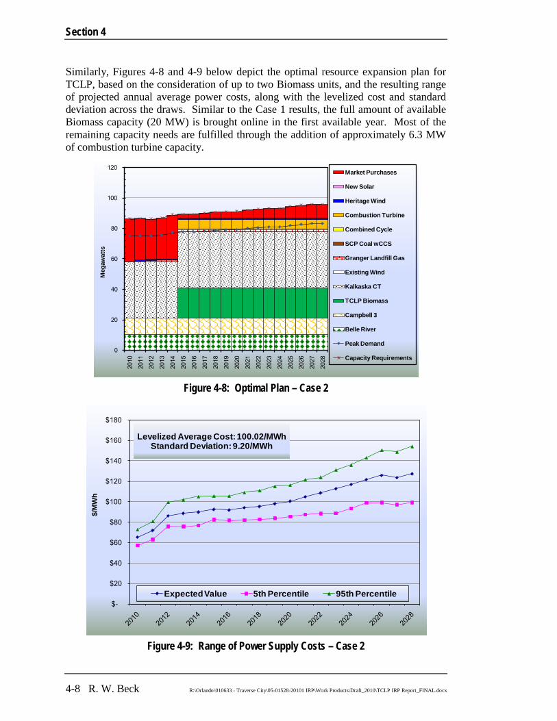
Section 4
4-8 R. W. Beck R:\Orlando\010633 - Traverse City\05-01528-20101 IRP\Work Products\Draft_2010\TCLP IRP Report_FINAL.docx
Similarly, Figures 4-8 and 4-9 below depict the optimal resource expansion plan for TCLP, based on the consideration of up to two Biomass units, and the resulting range of projected annual average power costs, along with the levelized cost and standard deviation across the draws. Similar to the Case 1 results, the full amount of available Biomass capacity (20 MW) is brought online in the first available year. Most of the remaining capacity needs are fulfilled through the addition of approximately 6.3 MW of combustion turbine capacity.
Figure 4-8: Optimal Plan – Case 2
Figure 4-9: Range of Power Supply Costs – Case 2
0
20
40
60
80
100
120
2010
2011
2012
2013
2014
2015
2016
2017
2018
2019
2020
2021
2022
2023
2024
2025
2026
2027
2028
Meg
awat
ts
Market Purchases
New Solar
Heritage Wind
Combustion Turbine
Combined Cycle
SCP Coal wCCS
Granger Landfill Gas
Existing Wind
Kalkaska CT
TCLP Biomass
Campbell 3
Belle River
Peak Demand
Capacity Requirements
$-
$20
$40
$60
$80
$100
$120
$140
$160
$180
$/M
Wh
Expected Value 5th Percentile 95th Percentile
Levelized Average Cost: 100.02/MWhStandard Deviation: 9.20/MWh
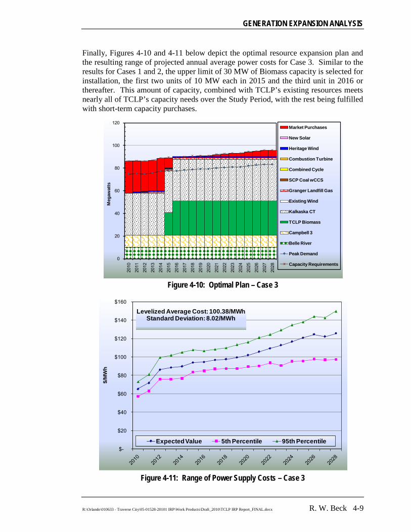
GENERATION EXPANSION ANALYSIS
R:\Orlando\010633 - Traverse City\05-01528-20101 IRP\Work Products\Draft_2010\TCLP IRP Report_FINAL.docx R. W. Beck 4-9
Finally, Figures 4-10 and 4-11 below depict the optimal resource expansion plan and the resulting range of projected annual average power costs for Case 3. Similar to the results for Cases 1 and 2, the upper limit of 30 MW of Biomass capacity is selected for installation, the first two units of 10 MW each in 2015 and the third unit in 2016 or thereafter. This amount of capacity, combined with TCLP’s existing resources meets nearly all of TCLP’s capacity needs over the Study Period, with the rest being fulfilled with short-term capacity purchases.
Figure 4-10: Optimal Plan – Case 3
Figure 4-11: Range of Power Supply Costs – Case 3
0
20
40
60
80
100
120 20
10
2011
2012
2013
2014
2015
2016
2017
2018
2019
2020
2021
2022
2023
2024
2025
2026
2027
2028
Meg
awat
ts
Market Purchases
New Solar
Heritage Wind
Combustion Turbine
Combined Cycle
SCP Coal wCCS
Granger Landfill Gas
Existing Wind
Kalkaska CT
TCLP Biomass
Campbell 3
Belle River
Peak Demand
Capacity Requirements
$-
$20
$40
$60
$80
$100
$120
$140
$160
$/M
Wh
Expected Value 5th Percentile 95th Percentile
Levelized Average Cost: 100.38/MWhStandard Deviation: 8.02/MWh

Section 4
4-10 R. W. Beck R:\Orlando\010633 - Traverse City\05-01528-20101 IRP\Work Products\Draft_2010\TCLP IRP Report_FINAL.docx
4.3.1 Sensitivity of Results to Higher Gas Prices The power market projections produced as part of this IRP Study were developed in June 2009, and some of the fuel price projections in early 2009. Since late 2008, natural gas prices have fallen, from a peak in 2008 of about $12/MMBtu to a more recent range of $4 - $6/MMBtu. However, it is uncertain whether these lower natural gas prices will be sustainable in the long-term, particularly given the potential for greenhouse gas legislation. The natural gas price forecast for the expected case reflects significantly higher gas prices than those experienced since late 2008 but considerably lower over the next several years than the mid-2008 period.
In order to assess the sensitivity of the Optimal Plans to higher and lower natural gas prices, Cases 1 through 3 (again corresponding to varying levels of maximum allowed Biomass capacity) were re-simulated with higher and lower natural gas prices, set to the 70th and 30th percentiles, respectively. The resulting gas prices correspond to levels at which gas prices are only 30% likely to be higher or lower, respectively. Under the High Gas Prices sensitivity case, gas prices are on average approximately 27% higher than the expected gas prices. Under the Low Gas Prices sensitivity case, gas prices are on average approximately 21% lower than the expected prices.
The results of this scenario showed that the Optimal Plans in each case were essentially unaffected by the High Gas Prices sensitivity. This is primarily because the Optimal Plans already resulted in essentially the maximum amount of Biomass capacity possible being selected. The Combustion Turbine capacity selected in Cases 1 and 2 were also unaffected, as the market is similarly influenced by natural gas prices as the operating costs of this technology. However, the resulting market prices are still not high enough to warrant the higher capital costs of building the SCP Coal with CCS resource or additional renewable resources.
The Low Gas Prices sensitivity resulted in Optimal Plans reflecting delays in the build-out of Biomass capacity. However, the ultimate amount of Biomass capacity that was reflected in the Optimal Plan was the same. Figure 4-12 provides an example, using the results of Case 2, which corresponds to a maximum allowed Biomass capacity of 20 MW. As compared to the results under expected gas prices, shown in Figure 4-8, the Optimal Plan under this sensitivity reflects only 10 MW of Biomass capacity added in 2015, with the remaining allowed 10 MW not built until 2026. The 6.3 MW of Combustion Turbine capacity is also added in 2015, as in the expected case. The Low Gas Prices sensitivity also reflects the market being relied upon for a greater share of capacity and energy needs.

GENERATION EXPANSION ANALYSIS
R:\Orlando\010633 - Traverse City\05-01528-20101 IRP\Work Products\Draft_2010\TCLP IRP Report_FINAL.docx R. W. Beck 4-11
Figure 4-12: Optimal Plan – Case 2 (Low Gas Prices Sensitivity)
4.3.2 Comparison of Optimal Plan Cases 1 – 3 Figure 4-13 below compares the expected annual power supply costs under the three Optimal Plan Cases discussed above as compared to the Existing Resources. The comparison shows that although the annual power costs are fairly close throughout much of the Study Period, the Optimal Plan Cases are projected to be significantly lower than the Existing Resources case beginning 2021. This is most likely the result of projected increases in the cost of CO2 emissions due to the reduction in the number of free allowances under the Lieberman-Warner carbon legislation.
0
20
40
60
80
100
120
2010
2011
2012
2013
2014
2015
2016
2017
2018
2019
2020
2021
2022
2023
2024
2025
2026
2027
2028
Meg
awat
ts
Market Purchases
New Solar
Heritage Wind
Combustion Turbine
Combined Cycle
SCP Coal wCCS
Granger Landfill Gas
Existing Wind
Kalkaska CT
TCLP Biomass
Campbell 3
Belle River
Peak Demand
Capacity Requirements

Section 4
4-12 R. W. Beck R:\Orlando\010633 - Traverse City\05-01528-20101 IRP\Work Products\Draft_2010\TCLP IRP Report_FINAL.docx
Figure 4-13: Expected Power Supply Costs
Figure 4-14 below provides a comparison of the three alternative expansion plans in the form of an X-Y chart, which combines both the levelized power cost over 2011-2028 for each plan and its standard deviation. The relative position of each plan along the X- and Y-axes corresponds to a trade-off between a preference for lower expected costs and a preference for projected costs of greater certainty (i.e., lower standard deviation), with points closer to the origin being overall more preferential. It is up to the utility planner to determine the acceptable trade-off between resource plans of lower cost versus those of lower uncertainty.
$-
$20
$40
$60
$80
$100
$120
$140
$160
2010
2011
2012
2013
2014
2015
2016
2017
2018
2019
2020
2021
2022
2023
2024
2025
2026
2027
2028
$/M
Wh
Existing Resources Optimal Plan - Case 1
Optimal Plan - Case 2 Optimal Plan - Case 3

GENERATION EXPANSION ANALYSIS
R:\Orlando\010633 - Traverse City\05-01528-20101 IRP\Work Products\Draft_2010\TCLP IRP Report_FINAL.docx R. W. Beck 4-13
Figure 4-14: Power Supply Costs Comparison
The results reflect that the Optimal Plans result in lower average levelized cost than the Existing Resources, and that they also successively lower the standard deviation of levelized power costs across the draws. The Optimal Plans add a significant amount of Biomass capacity, which both lowers the average levelized cost and significantly lowers the variability in levelized cost, which is evident in the lower standard deviation. This is most likely driven from the fact that the Biomass resource utilizes fuel that is subject to less volatility than gas-fired resources, based on the assumptions relied on herein, which also influence market prices more so than other fuel types.
Figure 4-15 below provides a similar comparison as that shown above. However, rather than charting the standard deviation on the Y-axis, the value on the Y-axis is the projected levelized power costs at the 95th percentile. This provides a measure of exposure to high power costs under each resource expansion case rather than simply how large the spread in potential costs might be (which includes the effects of both high and low cost uncertainty).
Similar to the conclusions associated with Figure 4-14 above, Figure 4-15 shows that the Optimal Plans generally result in successively lower levelized power costs on an expected value basis but also at the 95th percentile. This is most likely a function of the much greater stability of fuel costs of the Biomass resource, which are assumed to have similar volatility and uncertainty as coal prices, than market purchases.
7.6
8.4
9.2
10.0
10.8
11.6
12.4
99.5 100.0 100.5 101.0 101.5 102.0 102.5 103.0 103.5
Stan
dard
Dev
iatio
n
Levelized Cost ($/MWh)
Existing Resources Optimal Plan - Case 1
Optimal Plan - Case 2 Optimal Plan - Case 3

Section 4
4-14 R. W. Beck R:\Orlando\010633 - Traverse City\05-01528-20101 IRP\Work Products\Draft_2010\TCLP IRP Report_FINAL.docx
Figure 4-15: High-range of Potential Power Supply Costs
The overall results discussed above suggest that, given the resource options that have been considered and the assumptions discussed in Section 2, TCLP should consider building up to 20-30 MW of Biomass capacity to be brought online over 2015-2026. These units are intended to operate at high capacity factors, and indeed must be to support steam or hot water sales to which they would be tied. Given that amount of capacity and TCLP’s other resources, it is estimated that as much as 40% of the energy generated by this amount of Biomass capacity would be surplus to be sold into the wholesale market for the first several years of the Study Period. While the risks associated with this surplus energy are accounted for in the simulations that support the additions of Biomass capacity, TCLP should consider its tolerance for risk and perhaps limit its exposure somewhat. Accordingly, the Case 2 results, which consist of the additions of 20 MW of Biomass capacity and approximately 6.3 MW of Combustion Turbine capacity appear most reasonable and representative of balancing TCLP’s goals of lowest cost and minimizing risk, while also achieving the goal of a significant renewable generation percentage, as discussed below. Given the results of the Low Gas Prices sensitivity, TCLP might consider building a smaller amount of Biomass capacity in the 2015 timeframe and building additional capacity somewhat later. This would afford TCLP some flexibility in the event that the relatively low natural gas prices that are evident today appear likely to be sustained in the long-term.
Appendix D contains summary tables of the resulting load and resource balance and projected power supply costs for each of the three resource expansion plans over the period 2011 through 2028.
111.0
112.9
114.8
116.7
118.6
120.5
122.4
99.5 100.0 100.5 101.0 101.5 102.0 102.5 103.0 103.5
Up-
side
Cos
t ($/
MW
h)
Levelized Cost ($/MWh)
Existing Resources Optimal Plan - Case 1
Optimal Plan - Case 2 Optimal Plan - Case 3
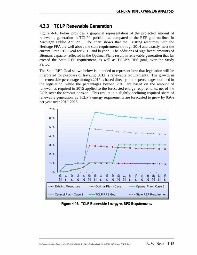
GENERATION EXPANSION ANALYSIS
R:\Orlando\010633 - Traverse City\05-01528-20101 IRP\Work Products\Draft_2010\TCLP IRP Report_FINAL.docx R. W. Beck 4-15
4.3.3 TCLP Renewable Generation Figure 4-16 below provides a graphical representation of the projected amount of renewable generation in TCLP’s portfolio as compared to the REP goal outlined in Michigan Public Act 295. The chart shows that the Existing resources with the Heritage PPA are well above the state requirements through 2014 and exactly meet the current State REP Goal for 2015 and beyond. The additions of significant amounts of Biomass capacity reflected in the Optimal Plans result in renewable generation that far exceed the State REP requirement, as well as TCLP’s RPS goal, over the Study Period.
The State REP Goal shown below is intended to represent how that legislation will be interpreted for purposes of tracking TCLP’s renewable requirements. The growth in the renewable percentage through 2015 is based directly on the percentages outlined in the legislation, while the percentages beyond 2015 are based on the amount of renewables required in 2015 applied to the forecasted energy requirements, net of the EOP, over the forecast horizon. This results in a slightly declining required share of renewable generation, as TCLP’s energy requirements are forecasted to grow by 0.9% per year over 2010-2028.
Figure 4-16: TCLP Renewable Energy vs RPS Requirements
0%
10%
20%
30%
40%
50%
60%
70%
2010
2011
2012
2013
2014
2015
2016
2017
2018
2019
2020
2021
2022
2023
2024
2025
2026
2027
2028
Existing Resources Optimal Plan - Case 1 Optimal Plan - Case 3
Optimal Plan - Case 2 TCLP RPS Goal State REP Requirement


Appendix A MISO EAST MARKET REPORT –
REGIONAL POWER PRICE FORECAST

App A - MISO East Market Report TCLP_20100210.doc 2/25/10 R. W. Beck A-1
Appendix A MISO EAST MARKET REPORT –
REGIONAL POWER PRICE FORECAST
A.1 Stochastic Market Module Description A.1.1 Overview For the IRP Study, the R. W. Beck proprietary Stochastic Econometric Regional Forecasting (“SERF”) model was used. The SERF model generates stochastic projections of fuel prices, electric loads for the region and the subject utility (in this case TCLP), emission prices, and power prices. The model simulates corresponding utility power supply costs for multiple potential resource expansion portfolios based on the stochastic projections. The Stochastic Market Module generates stochastic projections of fuel, power prices, utility loads, and emission prices and simulates the build-out and commitment/dispatch of market resources
A more detailed description of the SERF Model is included in Appendix C.
A.2 Market Module Inputs and Assumptions A.2.1 Study Period Price forecasts will be developed for a 20 year period beginning January 1, 2009 and ending December 31, 2028.
A.2.2 Time Periods On-peak hours are defined by hour ending 8:00 to 23:00 EST during week days, and off-peak hours are defined as all other hours. Summer months are defined as June through September of each year.
A.2.3 Escalation Factors R. W. Beck has based the capital and operation and maintenance cost escalation factors utilized in our power supply planning models on the Blue Chip Economic Indicators (BCEI) dated March 2009. The BCEI forecast reflects the impacts of the current economic recession and projects an inflation rate, as measured by the Consumer Price Index (CPI), of -0.8% for 2009. The economy is projected to contract significantly in 2009, with a recovery in 2010. The long-term average annual rate of inflation projected in the BCEI is 2.4%.

Appendix A
App A - MISO East Market Report TCLP_20100210.doc 2/25/10 A-2 R. W. Beck
With regard to capital cost escalation, R. W. Beck’s assumption is based on our Project Cost Estimator forecast, which is developed from future capital costs escalation rates included in recent construction contracts; materials, equipment, and labor cost indices projected by Global Insight, Inc.; and R. W. Beck’s experience in the industry. The current escalation adder for future capital costs is equal to our general inflation assumption discussed above for the duration of the Study Period.
A.2.4 Regions The Eastern interconnect power market model incorporates the regions shown in Figure A-1. The region of interest for Traverse City Light & Power is MISO East, which primarily comprises the utilities in Michigan, FirstEnergy in Ohio, and utilities in central and southern Indiana and Illinois. Each region is assumed to have a required reserve margin of 15%. Transmission transfer limits between the regions, in terms of both energy and capacity, were estimated by R. W. Beck transmission experts based on their familiarity with the regions.
PJM West
MISO East
MRO-NW
PJM East
TVA
NYPP
NEPOOL
Southeast
Entergy
SPP
Figure A-1: Eastern Interconnection Ball and Stick
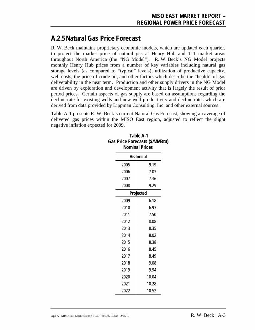
MISO EAST MARKET REPORT –
REGIONAL POWER PRICE FORECAST
App A - MISO East Market Report TCLP_20100210.doc 2/25/10 R. W. Beck A-3
A.2.5 Natural Gas Price Forecast R. W. Beck maintains proprietary economic models, which are updated each quarter, to project the market price of natural gas at Henry Hub and 111 market areas throughout North America (the “NG Model”). R. W. Beck’s NG Model projects monthly Henry Hub prices from a number of key variables including natural gas storage levels (as compared to “typical” levels), utilization of productive capacity, well costs, the price of crude oil, and other factors which describe the “health” of gas deliverability in the near term. Production and other supply drivers in the NG Model are driven by exploration and development activity that is largely the result of prior period prices. Certain aspects of gas supply are based on assumptions regarding the decline rate for existing wells and new well productivity and decline rates which are derived from data provided by Lippman Consulting, Inc. and other external sources.
Table A-1 presents R. W. Beck’s current Natural Gas Forecast, showing an average of delivered gas prices within the MISO East region, adjusted to reflect the slight negative inflation expected for 2009.
Table A-1 Gas Price Forecasts ($/MMBtu)
Nominal Prices
Historical 2005 9.19 2006 7.03 2007 7.36 2008 9.29
Projected 2009 6.18 2010 6.93 2011 7.50 2012 8.08 2013 8.35 2014 8.02 2015 8.38 2016 8.45 2017 8.49 2018 9.08 2019 9.94 2020 10.04 2021 10.28 2022 10.52
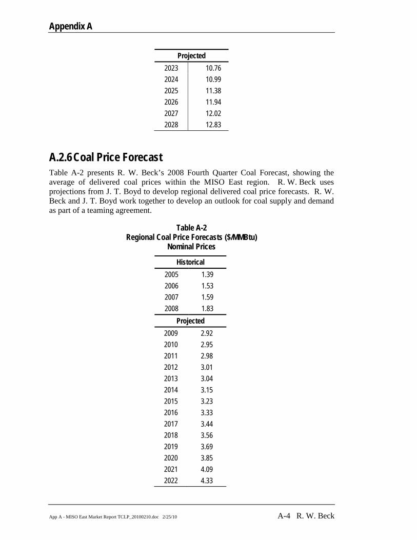
Appendix A
App A - MISO East Market Report TCLP_20100210.doc 2/25/10 A-4 R. W. Beck
Projected 2023 10.76 2024 10.99 2025 11.38 2026 11.94 2027 12.02 2028 12.83
A.2.6 Coal Price Forecast Table A-2 presents R. W. Beck’s 2008 Fourth Quarter Coal Forecast, showing the average of delivered coal prices within the MISO East region. R. W. Beck uses projections from J. T. Boyd to develop regional delivered coal price forecasts. R. W. Beck and J. T. Boyd work together to develop an outlook for coal supply and demand as part of a teaming agreement.
Table A-2 Regional Coal Price Forecasts ($/MMBtu)
Nominal Prices
Historical 2005 1.39 2006 1.53 2007 1.59 2008 1.83
Projected 2009 2.92 2010 2.95 2011 2.98 2012 3.01 2013 3.04 2014 3.15 2015 3.23 2016 3.33 2017 3.44 2018 3.56 2019 3.69 2020 3.85 2021 4.09 2022 4.33

MISO EAST MARKET REPORT –
REGIONAL POWER PRICE FORECAST
App A - MISO East Market Report TCLP_20100210.doc 2/25/10 R. W. Beck A-5
Projected 2023 4.57 2024 4.75 2025 4.92 2026 5.11 2027 5.29 2028 5.49
A.2.7 Emissions Allowance Price Projections SO2 and NOX
R. W. Beck has developed a proprietary SO2 and NOX allowance price forecasting model. This model is integrated with other energy market simulation models utilized by R. W. Beck.
Allowance Prices
The forecast is developed by simulating the operation of the U.S. power system over the Study Period using the PROMOD and MarketPower models developed by Ventyx. The emissions from each power plant unit are calculated and allowance prices are derived from simulated decisions to install emission control technologies on individual units. It is assumed that future allowance prices will be directly related to the cost of retrofitting units with emission control technologies.
A target emission level is assumed for each year so as to be compatible with current emission regulations. Total costs for installing and operating scrubber, selective catalytic reduction, selective non-catalytic reduction controls and low NOX burners are estimated for each generating unit from proprietary cost functions. This total cost expressed as an annual expense, divided by tons abated gives the annual dollars per ton cost. For each forecast year, decisions to install controls are simulated starting with the least cost units until the target emission level for the year is satisfied. The last unit to install controls determines the forecast allowance price for that year – the dollars per ton abatement cost is taken as the clearing price. The process and integration with other market simulation models is iterated until stable emissions clearing prices are reached.
The allowance prices that result from the model reflect costs at long-term equilibrium. Short- and medium-term market factors may cause spot and/or forward market allowance prices to deviate higher or lower from the equilibrium. So as to better represent the current market conditions, market forward and spot prices for SO2 and NOX allowances (to the extent they are available) are blended with the modeled equilibrium prices. Market prices are averaged with the modeled equilibrium price at various weightings to arrive at the final forecast prices. Weightings are determined based upon the amount of available forward data, with near term years weighted more heavily to the market price and later term years weighted more heavily to the modeled

Appendix A
App A - MISO East Market Report TCLP_20100210.doc 2/25/10 A-6 R. W. Beck
equilibrium price. Prices for years beyond available market data are the modeled equilibrium price from the model.
CO2
R. W. Beck has a proprietary green house gas (“GHG”) model that captures the relationship between CO2 allowance prices, power demand and prices, natural gas demand and prices, and other fuel demand and prices. This market simulation model divides the U.S. into multiple interconnected regions, simulates the retirement of existing units if they are not profitable, and constructs new replacement units to meet reserve requirements. The potential build out of new units includes traditional fossil-fueled technologies (coal-fired supercritical, natural gas-fired combined cycle, and combustion turbines) and also nuclear generation, wind and solar generation, and new technologies such as coal generation with carbon capture and sequestration. The model simulates the energy industry response to an assumed CO2 allowance price, including gas consumption (and gas price response), CO2 emissions, and demand response. The model iterates on the CO2 allowance price until a balanced gas consumption/gas price/load demand response solution is obtained that meets the required power sector CO2 reductions based on a national GHG target.
Allowance Prices
The projected new generating resource capital costs and operating costs and characteristics are developed in conjunction with R. W. Beck’s Global Asset Consulting practice. Our engineers have experience in all power generation technologies, have projected new technology costs, and have compiled a database with information on costs related to construction and financing of new units.
Our carbon model reflects the potential reductions in the power sector, but anticipated future federal legislation will likely create a national market that crosses all sectors. Many cost effective measures, both on the demand-side of the power sector and in other sectors, can be implemented before supply-side solutions in the power industry (retrofitting existing plants, retiring existing coal-fired generation, building nuclear, and carbon capture and sequestration) become competitive.
At the point when power sector supply-side measures are required to meet mandated GHG reductions, their control costs will begin to set the marginal price for allowances. Early on, carbon reductions will most likely come from other sectors, and the power sector will be a net purchaser of allowances. Within our model, we assume that, over time, CO2 allowance prices will increase to the power sector marginal costs as power sector supply side options are needed for further carbon reductions.
CO2
Based on recent legislation that has gone through extensive debate in the U.S. Senate process, which is representative of regional concerns, many of the plans allow for some percentage of the allowances to be freely allocated and the remainder to be auctioned. Free allowances represent an opportunity cost and based on evidence from the Acid Rain program and the EU-ETS program, generators do not pass on the savings from them. Instead, they bid in full emission costs and either use the free
Allocations
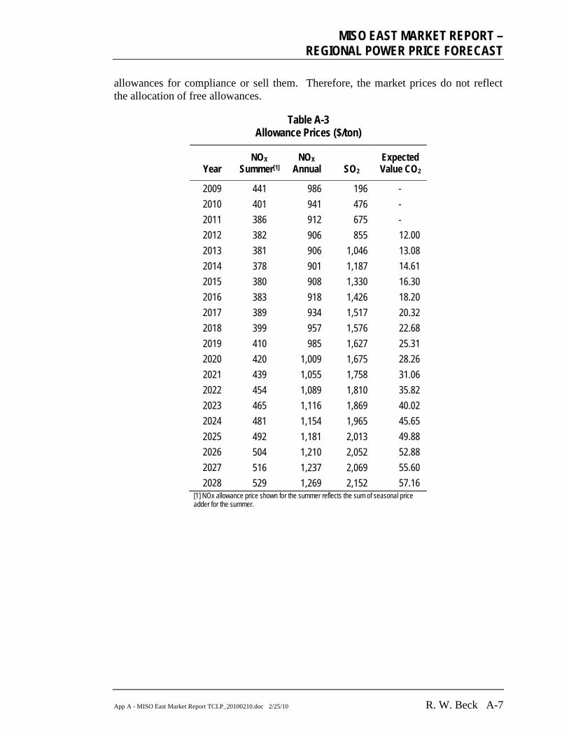
MISO EAST MARKET REPORT –
REGIONAL POWER PRICE FORECAST
App A - MISO East Market Report TCLP_20100210.doc 2/25/10 R. W. Beck A-7
allowances for compliance or sell them. Therefore, the market prices do not reflect the allocation of free allowances.
Table A-3 Allowance Prices ($/ton)
Year NOX
SummerNO
[1] X
SO
Annual Expected Value CO2
2009
2
441 986 196 - 2010 401 941 476 - 2011 386 912 675 - 2012 382 906 855 12.00 2013 381 906 1,046 13.08 2014 378 901 1,187 14.61 2015 380 908 1,330 16.30 2016 383 918 1,426 18.20 2017 389 934 1,517 20.32 2018 399 957 1,576 22.68 2019 410 985 1,627 25.31 2020 420 1,009 1,675 28.26 2021 439 1,055 1,758 31.06 2022 454 1,089 1,810 35.82 2023 465 1,116 1,869 40.02 2024 481 1,154 1,965 45.65 2025 492 1,181 2,013 49.88 2026 504 1,210 2,052 52.88 2027 516 1,237 2,069 55.60 2028 529 1,269 2,152 57.16
[1] NOx allowance price shown for the summer reflects the sum of seasonal price adder for the summer.
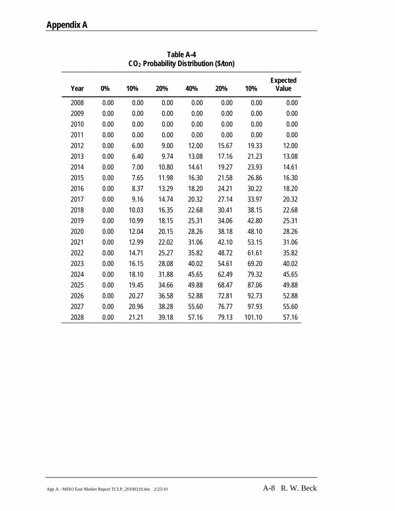
Appendix A
App A - MISO East Market Report TCLP_20100210.doc 2/25/10 A-8 R. W. Beck
Table A-4 CO2
Year
Probability Distribution ($/ton)
0% 10% 20% 40% 20% 10% Expected
Value
2008 0.00 0.00 0.00 0.00 0.00 0.00 0.00 2009 0.00 0.00 0.00 0.00 0.00 0.00 0.00 2010 0.00 0.00 0.00 0.00 0.00 0.00 0.00 2011 0.00 0.00 0.00 0.00 0.00 0.00 0.00 2012 0.00 6.00 9.00 12.00 15.67 19.33 12.00 2013 0.00 6.40 9.74 13.08 17.16 21.23 13.08 2014 0.00 7.00 10.80 14.61 19.27 23.93 14.61 2015 0.00 7.65 11.98 16.30 21.58 26.86 16.30 2016 0.00 8.37 13.29 18.20 24.21 30.22 18.20 2017 0.00 9.16 14.74 20.32 27.14 33.97 20.32 2018 0.00 10.03 16.35 22.68 30.41 38.15 22.68 2019 0.00 10.99 18.15 25.31 34.06 42.80 25.31 2020 0.00 12.04 20.15 28.26 38.18 48.10 28.26 2021 0.00 12.99 22.02 31.06 42.10 53.15 31.06 2022 0.00 14.71 25.27 35.82 48.72 61.61 35.82 2023 0.00 16.15 28.08 40.02 54.61 69.20 40.02 2024 0.00 18.10 31.88 45.65 62.49 79.32 45.65 2025 0.00 19.45 34.66 49.88 68.47 87.06 49.88 2026 0.00 20.27 36.58 52.88 72.81 92.73 52.88 2027 0.00 20.96 38.28 55.60 76.77 97.93 55.60 2028 0.00 21.21 39.18 57.16 79.13 101.10 57.16
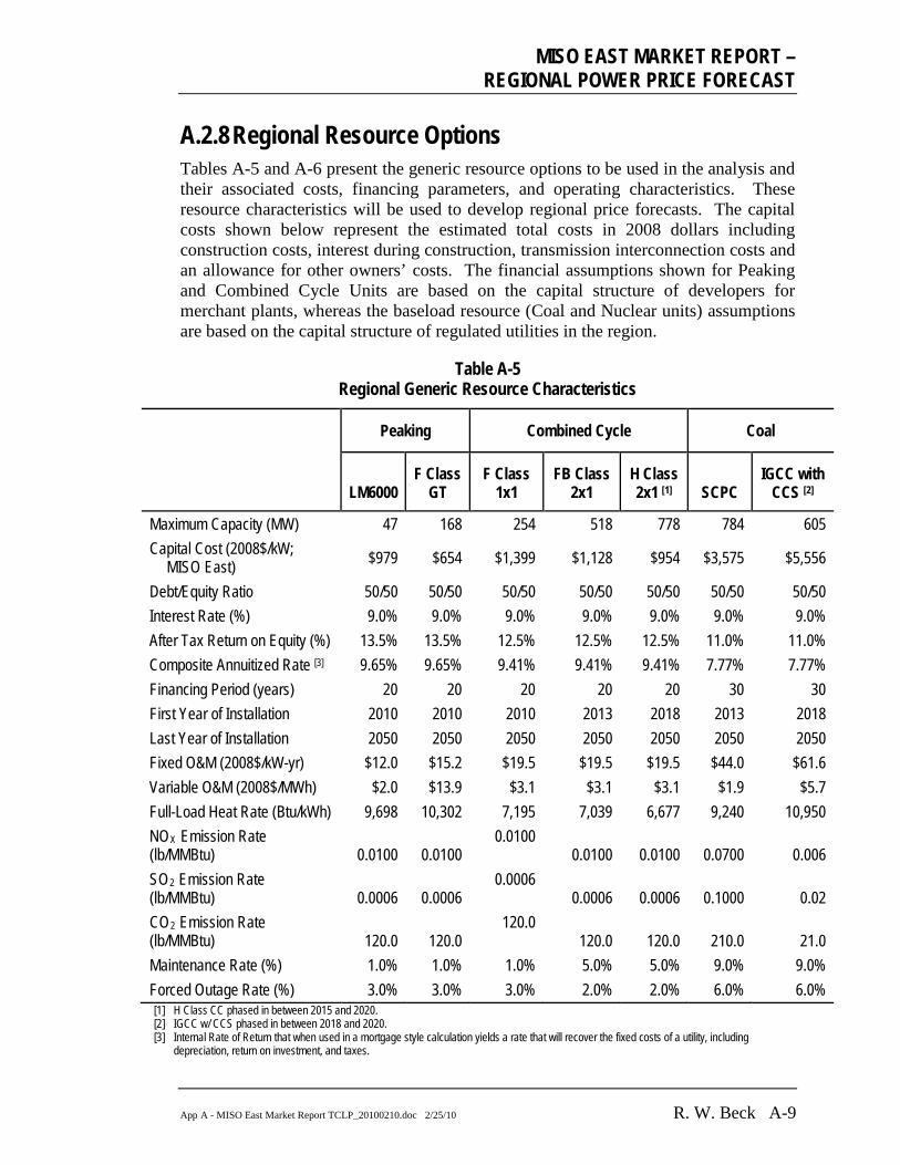
MISO EAST MARKET REPORT –
REGIONAL POWER PRICE FORECAST
App A - MISO East Market Report TCLP_20100210.doc 2/25/10 R. W. Beck A-9
A.2.8 Regional Resource Options Tables A-5 and A-6 present the generic resource options to be used in the analysis and their associated costs, financing parameters, and operating characteristics. These resource characteristics will be used to develop regional price forecasts. The capital costs shown below represent the estimated total costs in 2008 dollars including construction costs, interest during construction, transmission interconnection costs and an allowance for other owners’ costs. The financial assumptions shown for Peaking and Combined Cycle Units are based on the capital structure of developers for merchant plants, whereas the baseload resource (Coal and Nuclear units) assumptions are based on the capital structure of regulated utilities in the region.
Table A-5 Regional Generic Resource Characteristics
Peaking Combined Cycle Coal
LM6000 F Class
GT F Class
1x1 FB Class
2x1 H Class 2x1 SCPC [1]
IGCC with CCS
Maximum Capacity (MW)
[2]
47 168 254 518 778 784 605 Capital Cost (2008$/kW; MISO East) $979 $654 $1,399 $1,128 $954 $3,575 $5,556
Debt/Equity Ratio 50/50 50/50 50/50 50/50 50/50 50/50 50/50 Interest Rate (%) 9.0% 9.0% 9.0% 9.0% 9.0% 9.0% 9.0% After Tax Return on Equity (%) 13.5% 13.5% 12.5% 12.5% 12.5% 11.0% 11.0% Composite Annuitized Rate 9.65% [3] 9.65% 9.41% 9.41% 9.41% 7.77% 7.77% Financing Period (years) 20 20 20 20 20 30 30 First Year of Installation 2010 2010 2010 2013 2018 2013 2018 Last Year of Installation 2050 2050 2050 2050 2050 2050 2050 Fixed O&M (2008$/kW-yr) $12.0 $15.2 $19.5 $19.5 $19.5 $44.0 $61.6 Variable O&M (2008$/MWh) $2.0 $13.9 $3.1 $3.1 $3.1 $1.9 $5.7 Full-Load Heat Rate (Btu/kWh) 9,698 10,302 7,195 7,039 6,677 9,240 10,950 NOX
0.0100 Emission Rate
(lb/MMBtu) 0.0100 0.0100
0.0100 0.0100 0.0700 0.006 SO2
0.0006 Emission Rate
(lb/MMBtu) 0.0006 0.0006
0.0006 0.0006 0.1000 0.02 CO2
120.0 Emission Rate
(lb/MMBtu) 120.0 120.0
120.0 120.0 210.0 21.0 Maintenance Rate (%) 1.0% 1.0% 1.0% 5.0% 5.0% 9.0% 9.0% Forced Outage Rate (%) 3.0% 3.0% 3.0% 2.0% 2.0% 6.0% 6.0% [1] H Class CC phased in between 2015 and 2020. [2] IGCC w/ CCS phased in between 2018 and 2020. [3] Internal Rate of Return that when used in a mortgage style calculation yields a rate that will recover the fixed costs of a utility, including
depreciation, return on investment, and taxes.
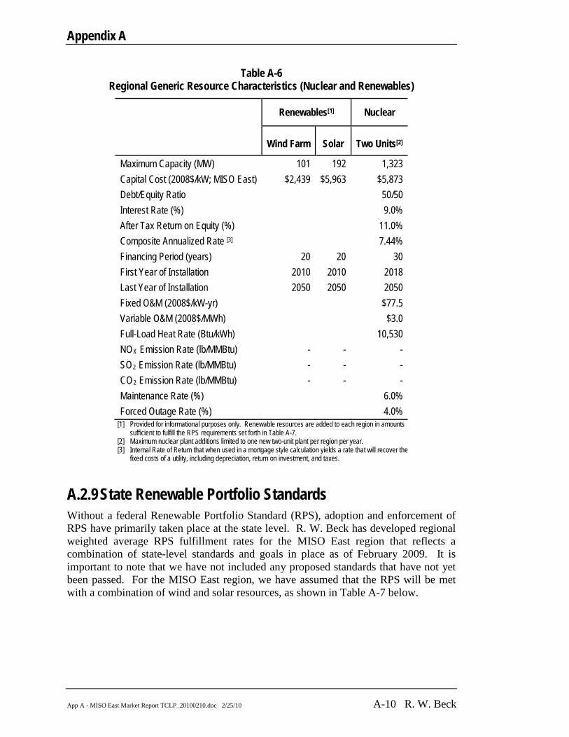
Appendix A
App A - MISO East Market Report TCLP_20100210.doc 2/25/10 A-10 R. W. Beck
Table A-6 Regional Generic Resource Characteristics (Nuclear and Renewables)
Renewables Nuclear [1]
Wind Farm Solar Two Units
Maximum Capacity (MW)
[2]
101 192 1,323 Capital Cost (2008$/kW; MISO East) $2,439 $5,963 $5,873 Debt/Equity Ratio 50/50 Interest Rate (%) 9.0% After Tax Return on Equity (%) 11.0% Composite Annualized Rate [3] 7.44% Financing Period (years) 20 20 30 First Year of Installation 2010 2010 2018 Last Year of Installation 2050 2050 2050 Fixed O&M (2008$/kW-yr) $77.5 Variable O&M (2008$/MWh) $3.0 Full-Load Heat Rate (Btu/kWh) 10,530 NOX - Emission Rate (lb/MMBtu) - - SO2 - Emission Rate (lb/MMBtu) - - CO2 - Emission Rate (lb/MMBtu) - - Maintenance Rate (%) 6.0% Forced Outage Rate (%) 4.0%
[1] Provided for informational purposes only. Renewable resources are added to each region in amounts sufficient to fulfill the RPS requirements set forth in Table A-7.
[2] Maximum nuclear plant additions limited to one new two-unit plant per region per year. [3] Internal Rate of Return that when used in a mortgage style calculation yields a rate that will recover the
fixed costs of a utility, including depreciation, return on investment, and taxes.
A.2.9 State Renewable Portfolio Standards Without a federal Renewable Portfolio Standard (RPS), adoption and enforcement of RPS have primarily taken place at the state level. R. W. Beck has developed regional weighted average RPS fulfillment rates for the MISO East region that reflects a combination of state-level standards and goals in place as of February 2009. It is important to note that we have not included any proposed standards that have not yet been passed. For the MISO East region, we have assumed that the RPS will be met with a combination of wind and solar resources, as shown in Table A-7 below.

MISO EAST MARKET REPORT –
REGIONAL POWER PRICE FORECAST
App A - MISO East Market Report TCLP_20100210.doc 2/25/10 R. W. Beck A-11
Table A-7 Assumed RPS Fulfillment Rates for the MISO East Region
Year Wind
Resources Solar
Resources 2009 1.2% 0.02% 2010 2.3% 0.04% 2011 3.5% 0.05% 2012 4.7% 0.07% 2013 5.9% 0.09% 2014 7.0% 0.11% 2015 8.2% 0.13% 2016 9.0% 0.14% 2017 9.9% 0.16% 2018 10.7% 0.18% 2019 11.5% 0.20% 2020 12.3% 0.22% 2021 12.8% 0.24% 2022 13.2% 0.24% 2023 13.7% 0.25% 2024 14.1% 0.26% 2025 14.5% 0.26% 2026 14.5% 0.26% 2027 14.5% 0.26% 2028 14.5% 0.26%
The development of the weighted average fulfillment rates shown in Table A-7 are based on documented by-state RPS goals in certain key years of the Study Period, with the interim years reflecting a linear interpolation between the key years. Goals outlined for key years have been averaged with pre-existing goals already in place for states within each region, based upon a weighted average of states within each region. For MISO East, the states of Michigan (10% RPS by 2015), Illinois (25% RPS by 2025), Indiana (20% RPS by 2020), Missouri (13% by 2021 with 2.0% solar), and Ohio (12.5% RPS by 2025 with 0.5% solar) have RPS goals, while the other states that comprise a very small portion of the region do not currently have RPS goals, netting an average fulfillment rate in 2025 of approximately 14.75%, which includes a small portion of solar and is assumed to perpetuate into the future.

Appendix A
App A - MISO East Market Report TCLP_20100210.doc 2/25/10 A-12 R. W. Beck
A.3 Market Module Results A.3.1 Stochastic Gas Price Forecasts The following graphs show the results of the 50 draws of the average annual gas prices from the Monte Carlo simulations of the regional model for the MISO East region. The bold black lines depict the 95th percentile values, expected values and 5th percentile values over the period 2009-2028.
MISO East Gas Prices
$0
$5
$10
$15
$20
$25
$30
$35
$40
2008
2009
2010
2011
2012
2013
2014
2015
2016
2017
2018
2019
2020
2021
2022
2023
2024
2025
2026
2027
2028
($/M
MB
tu)
Figure A-2: MISO East Gas Prices
A.3.2 Stochastic Coal Price Forecasts The following graphs show the results of the 50 draws of the average annual coal prices from the Monte Carlo simulations of the regional model for the MISO East region. The bold black lines depict the 95th percentile values, expected values and 5th percentile values over the period 2009-2028.
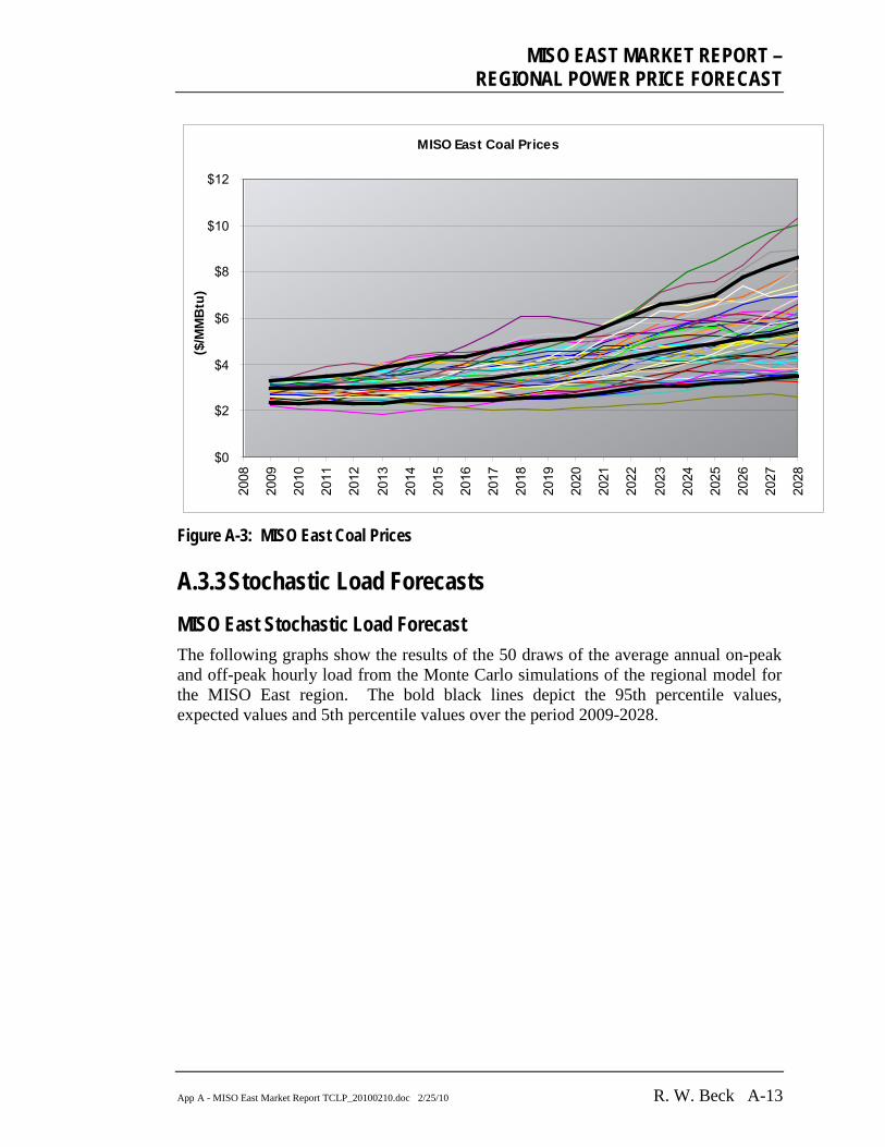
MISO EAST MARKET REPORT –
REGIONAL POWER PRICE FORECAST
App A - MISO East Market Report TCLP_20100210.doc 2/25/10 R. W. Beck A-13
MISO East Coal Prices
$0
$2
$4
$6
$8
$10
$12
2008
2009
2010
2011
2012
2013
2014
2015
2016
2017
2018
2019
2020
2021
2022
2023
2024
2025
2026
2027
2028
($/M
MB
tu)
Figure A-3: MISO East Coal Prices
A.3.3 Stochastic Load Forecasts MISO East Stochastic Load Forecast The following graphs show the results of the 50 draws of the average annual on-peak and off-peak hourly load from the Monte Carlo simulations of the regional model for the MISO East region. The bold black lines depict the 95th percentile values, expected values and 5th percentile values over the period 2009-2028.

Appendix A
App A - MISO East Market Report TCLP_20100210.doc 2/25/10 A-14 R. W. Beck
MISO East On-Peak Average Hourly Load
0
10,000
20,000
30,000
40,000
50,000
60,000
70,000
80,000
90,000
2008
2009
2010
2011
2012
2013
2014
2015
2016
2017
2018
2019
2020
2021
2022
2023
2024
2025
2026
2027
2028
2029
aMW
Figure A-4: MISO East On-Peak Average Hourly Load
MISO East Off-Peak Average Hourly Load
0
10,000
20,000
30,000
40,000
50,000
60,000
70,000
2008
2009
2010
2011
2012
2013
2014
2015
2016
2017
2018
2019
2020
2021
2022
2023
2024
2025
2026
2027
2028
2029
aMW
Figure A-5: MISO East Off-Peak Average Hourly Load
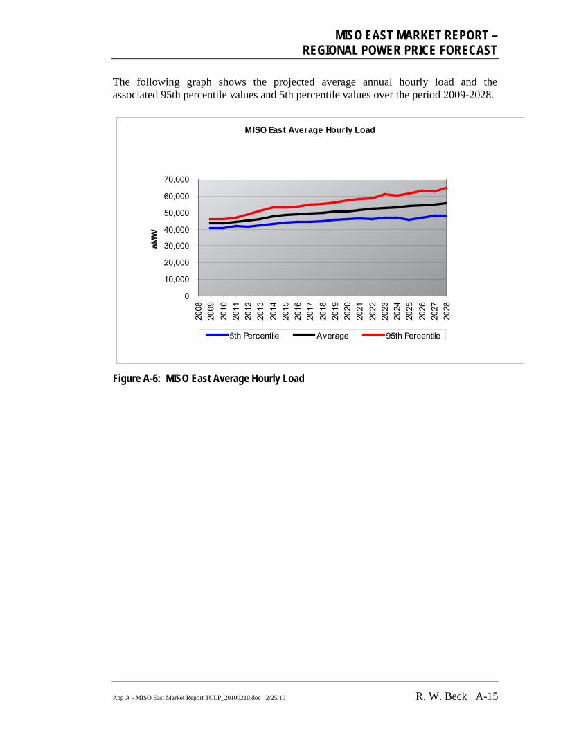
MISO EAST MARKET REPORT –
REGIONAL POWER PRICE FORECAST
App A - MISO East Market Report TCLP_20100210.doc 2/25/10 R. W. Beck A-15
The following graph shows the projected average annual hourly load and the associated 95th percentile values and 5th percentile values over the period 2009-2028.
MISO East Average Hourly Load
0
10,000
20,000
30,000
40,000
50,000
60,000
70,000
2008
2009
2010
2011
2012
2013
2014
2015
2016
2017
2018
2019
2020
2021
2022
2023
2024
2025
2026
2027
2028
aMW
5th Percentile Average 95th Percentile
Figure A-6: MISO East Average Hourly Load
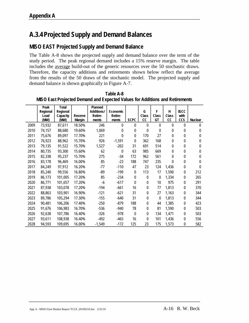
Appendix A
App A - MISO East Market Report TCLP_20100210.doc 2/25/10 A-16 R. W. Beck
A.3.4 Projected Supply and Demand Balances MISO EAST Projected Supply and Demand Balance The Table A-8 shows the projected supply and demand balance over the term of the study period. The peak regional demand includes a 15% reserve margin. The table includes the average
Table A-8 MISO East Projected Demand and Expected Values for Additions and Retirements
build-out of the generic resources over the 50 stochastic draws. Therefore, the capacity additions and retirements shown below reflect the average from the results of the 50 draws of the stochastic model. The projected supply and demand balance is shown graphically in Figure A-7.
Peak Regional
Load (MW)
Total Regional Capacity
(MW) Reserve Margin
Planned Additions/
Retire-ments
Economic Retire-ments SCPC
G Class
CC
F Class
GT
H Class
CC
IGCC with CCS Nuclear
2009 73,932 87,611 18.50% 246 0 0 0 0 0 0 0 2010 74,157 88,680 19.60% 1,069 0 0 0 0 0 0 0 2011 75,676 89,097 17.70% 221 0 0 170 27 0 0 0 2012 76,923 88,962 15.70% 926 -1,591 0 362 168 0 0 0 2013 79,135 91,522 15.70% 1,527 -202 31 691 514 0 0 0 2014 80,735 93,300 15.60% 62 0 63 985 669 0 0 0 2015 82,338 95,237 15.70% 275 -34 172 962 561 0 0 0 2016 83,178 96,469 16.00% 85 -23 188 747 235 0 0 0 2017 84,249 97,912 16.20% -77 -110 47 23 124 1,436 0 0 2018 85,240 99,556 16.80% -89 -199 0 113 17 1,590 0 212 2019 86,173 101,005 17.20% 85 -234 0 0 0 1,334 0 265 2020 86,771 101,657 17.20% -6 -617 0 0 10 975 0 291 2021 87,938 103,078 17.20% -194 -661 16 0 77 1,813 0 370 2022 88,863 103,901 16.90% -121 -621 31 0 27 1,163 0 344 2023 89,786 105,294 17.30% -155 -640 31 0 0 1,813 0 344 2024 90,481 106,206 17.40% -250 -879 188 0 44 1,385 0 423 2025 91,676 106,983 16.70% -536 -940 78 0 81 1,590 0 503 2026 92,638 107,786 16.40% -326 -978 0 0 134 1,471 0 503 2027 93,611 108,938 16.40% -492 -465 16 0 101 1,436 0 556 2028 94,593 109,695 16.00% -1,549 -172 125 23 175 1,573 0 582
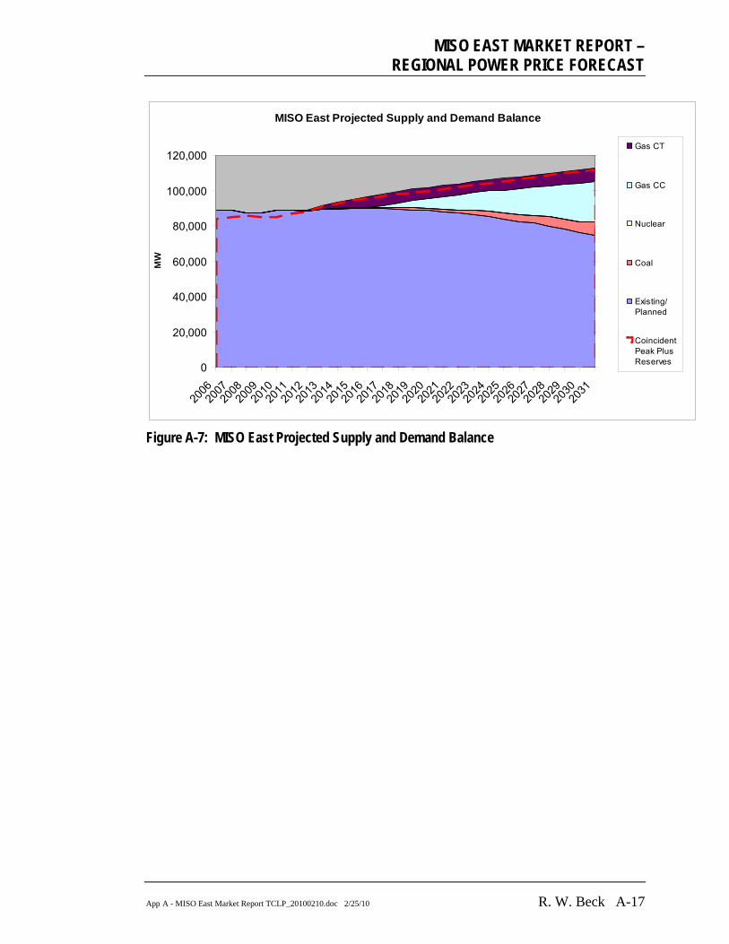
MISO EAST MARKET REPORT –
REGIONAL POWER PRICE FORECAST
App A - MISO East Market Report TCLP_20100210.doc 2/25/10 R. W. Beck A-17
MISO East Projected Supply and Demand Balance
0
20,000
40,000
60,000
80,000
100,000
120,000
2006
200720
0820
0920
1020
1120
1220
1320
1420
1520
1620
1720
1820
1920
2020
2120
2220
2320
2420
2520
2620
2720
2820
2920
3020
31
MW
0
20,000
40,000
60,000
80,000
100,000
120,000Gas CT
Gas CC
Nuclear
Coal
Existing/Planned
CoincidentPeak PlusReserves
Figure A-7: MISO East Projected Supply and Demand Balance
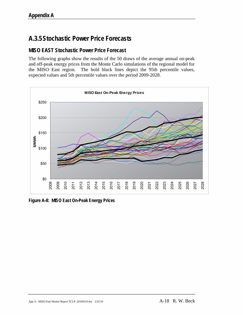
Appendix A
App A - MISO East Market Report TCLP_20100210.doc 2/25/10 A-18 R. W. Beck
A.3.5 Stochastic Power Price Forecasts MISO EAST Stochastic Power Price Forecast The following graphs show the results of the 50 draws of the average annual on-peak and off-peak energy prices from the Monte Carlo simulations of the regional model for the MISO East region. The bold black lines depict the 95th percentile values, expected values and 5th percentile values over the period 2009-2028.
MISO East On-Peak Energy Prices
$0
$50
$100
$150
$200
$250
2008
2009
2010
2011
2012
2013
2014
2015
2016
2017
2018
2019
2020
2021
2022
2023
2024
2025
2026
2027
2028
$/M
Wh
Figure A-8: MISO East On-Peak Energy Prices
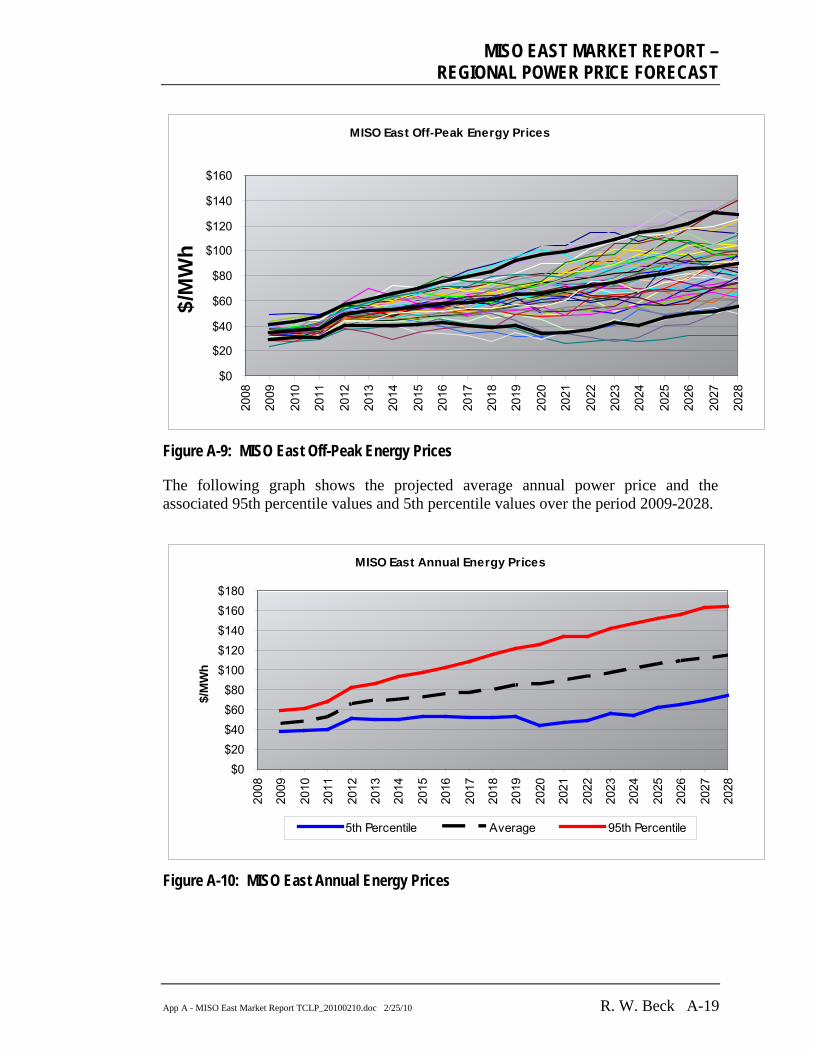
MISO EAST MARKET REPORT –
REGIONAL POWER PRICE FORECAST
App A - MISO East Market Report TCLP_20100210.doc 2/25/10 R. W. Beck A-19
MISO East Off-Peak Energy Prices
$0
$20
$40
$60
$80
$100
$120
$140
$160
2008
2009
2010
2011
2012
2013
2014
2015
2016
2017
2018
2019
2020
2021
2022
2023
2024
2025
2026
2027
2028
$/M
Wh
Figure A-9: MISO East Off-Peak Energy Prices
The following graph shows the projected average annual power price and the associated 95th percentile values and 5th percentile values over the period 2009-2028.
MISO East Annual Energy Prices
$0$20$40$60$80
$100$120$140$160$180
2008
2009
2010
2011
2012
2013
2014
2015
2016
2017
2018
2019
2020
2021
2022
2023
2024
2025
2026
2027
2028
$/M
Wh
5th Percentile Average 95th Percentile
Figure A-10: MISO East Annual Energy Prices

Appendix A
App A - MISO East Market Report TCLP_20100210.doc 2/25/10 A-20 R. W. Beck
The expected values of the on-peak, off-peak and average annual power price forecasts and the associated 95th percentile values and 5th percentile values for the average annual power price forecast over the period 2009-2028 are shown in the table below.
Table A-9 MISO East Expected Annual Energy Prices - $/MWh
Year Average On-Peak
Average Off-Peak
Average Annual Expected 5th % 95th %
2009 58.59 34.53 46.00 37.28 59.43 2010 61.47 36.03 48.16 39.06 61.40 2011 67.07 38.09 51.85 40.37 67.79 2012 83.98 49.39 65.84 50.98 82.30 2013 87.17 51.63 68.57 50.31 86.86 2014 87.50 53.18 69.54 50.47 93.53 2015 91.19 55.45 72.49 53.40 97.41 2016 94.28 57.66 75.07 53.37 101.83 2017 96.95 59.19 77.12 52.61 109.31 2018 100.46 60.95 79.79 52.07 115.63 2019 107.10 64.65 84.89 53.54 120.83 2020 108.22 65.81 86.05 44.43 125.59 2021 111.63 68.60 89.11 46.83 133.56 2022 117.42 72.09 93.61 49.25 132.94 2023 121.50 75.10 97.14 55.21 142.06 2024 125.23 78.15 100.62 54.11 146.34 2025 130.70 82.18 105.31 62.40 152.02 2026 135.24 85.39 109.16 66.08 155.55 2027 137.46 86.32 110.70 69.23 162.79 2028 143.37 89.33 114.92 74.19 163.92

MISO EAST MARKET REPORT –
REGIONAL POWER PRICE FORECAST
App A - MISO East Market Report TCLP_20100210.doc 2/25/10 R. W. Beck A-21
The expected values of the annual capacity prices and average annual power price (including the capacity component) are shown in the table below.
Table A-10 MISO East Expected Annual Power Prices
Year
Capacity Price
($/kW-yr)
Average Power Price
($/MWh) 2009 0.00 46.00 2010 0.00 48.16 2011 10.85 54.33 2012 48.57 76.72 2013 48.99 79.60 2014 43.79 79.38 2015 51.62 84.08 2016 33.34 82.55 2017 23.31 82.38 2018 18.87 84.07 2019 21.21 89.72 2020 11.30 88.61 2021 30.08 95.96 2022 19.48 98.04 2023 21.52 102.04 2024 20.48 105.27 2025 33.70 112.95 2026 35.32 117.14 2027 34.43 118.48 2028 39.10 123.71


Appendix B BIOMASS FUEL SUPPLY ANALYSIS

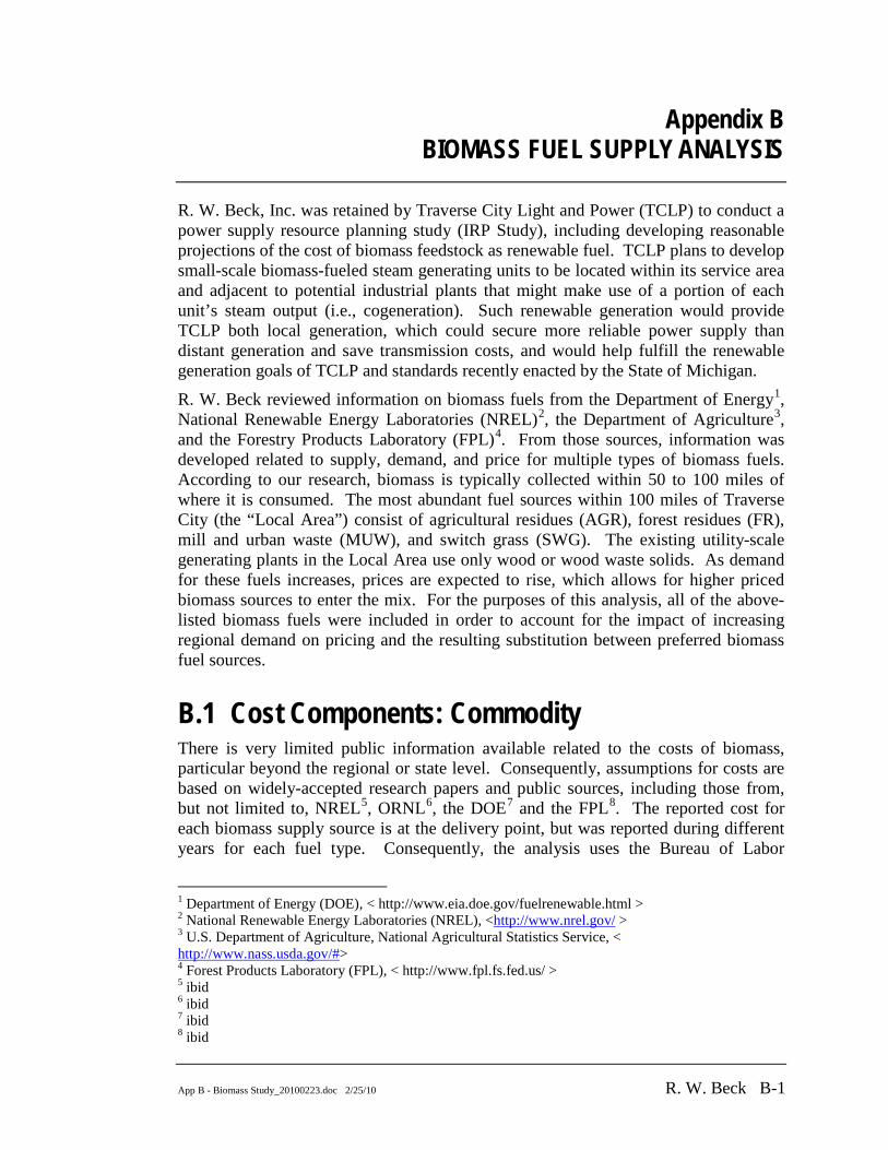
App B - Biomass Study_20100223.doc 2/25/10 R. W. Beck B-1
Appendix B BIOMASS FUEL SUPPLY ANALYSIS
R. W. Beck, Inc. was retained by Traverse City Light and Power (TCLP) to conduct a power supply resource planning study (IRP Study), including developing reasonable projections of the cost of biomass feedstock as renewable fuel. TCLP plans to develop small-scale biomass-fueled steam generating units to be located within its service area and adjacent to potential industrial plants that might make use of a portion of each unit’s steam output (i.e., cogeneration). Such renewable generation would provide TCLP both local generation, which could secure more reliable power supply than distant generation and save transmission costs, and would help fulfill the renewable generation goals of TCLP and standards recently enacted by the State of Michigan.
R. W. Beck reviewed information on biomass fuels from the Department of Energy1, National Renewable Energy Laboratories (NREL)2, the Department of Agriculture3, and the Forestry Products Laboratory (FPL)4
B.1 Cost Components: Commodity
. From those sources, information was developed related to supply, demand, and price for multiple types of biomass fuels. According to our research, biomass is typically collected within 50 to 100 miles of where it is consumed. The most abundant fuel sources within 100 miles of Traverse City (the “Local Area”) consist of agricultural residues (AGR), forest residues (FR), mill and urban waste (MUW), and switch grass (SWG). The existing utility-scale generating plants in the Local Area use only wood or wood waste solids. As demand for these fuels increases, prices are expected to rise, which allows for higher priced biomass sources to enter the mix. For the purposes of this analysis, all of the above-listed biomass fuels were included in order to account for the impact of increasing regional demand on pricing and the resulting substitution between preferred biomass fuel sources.
There is very limited public information available related to the costs of biomass, particular beyond the regional or state level. Consequently, assumptions for costs are based on widely-accepted research papers and public sources, including those from, but not limited to, NREL5, ORNL6, the DOE7 and the FPL8
1 Department of Energy (DOE), < http://www.eia.doe.gov/fuelrenewable.html >
. The reported cost for each biomass supply source is at the delivery point, but was reported during different years for each fuel type. Consequently, the analysis uses the Bureau of Labor
2 National Renewable Energy Laboratories (NREL), <http://www.nrel.gov/ > 3 U.S. Department of Agriculture, National Agricultural Statistics Service, < http://www.nass.usda.gov/#> 4 Forest Products Laboratory (FPL), < http://www.fpl.fs.fed.us/ > 5 ibid 6 ibid 7 ibid 8 ibid

Appendix B
App B - Biomass Study_20100223.doc 2/25/10 B-2 R. W. Beck
Statistics price index for logging and pulpwood to normalize the costs of each fuel type to 2008 dollars. R. W. Beck’s general inflation assumption of 2.4% is embedded in the annual forecast, but we have also considered other demand-side factors, which would impact future prices of the commodity, namely those related to fulfillment of the renewable portfolio standard (RPS) goals outlined in recent legislation enacted by the State of Michigan.
B.2 Cost Components: Demand Table B-1 lists existing biomass generation resources in the Local Area, which utilize a mix of wood and wood-waste solids (WDS) fuel sources. For the scope of this analysis, we have only identified the local competition for biomass sources as generating plants with an operating or planned unit status and have not included other competing uses for the fuel that may arise due to new standards for renewable resources. Furthermore, we have not identified the specific fuel classified under WDS, but a mix of paper pellets, railroad ties, wood chips or forest residues would generally be classified as WDS. This is consistent with standard classification systems used by NREL and Oakridge National Laboratories (ORNL). The analysis assumes that the existing plants will compete for the same biomass supply resources as the TCLP’s planned projects (5-10 MW installations totaling up to 30 MW over the study period). New capacity is assumed to operate at an 80% capacity factor (CF). Steam and hot-water production for resale are not included in this analysis.
Table B-1 Existing Local Area Biomass Generation
Plant Name County Capacity
(MW) Average Heat Rate
(MMBtu/MWh)
Cadillac Renewable Energy Wexford 39.6 17.69 Grayling (MI) Crawford 36.2 14.34 Hillman Power Co LLC Montmorency 17.8 14.55 Viking Energy of Lincoln Alcona 16 12.93 Viking Energy of McBain Missaukee 18 14.49
Existing generating resources in the Local Area comprise a total of 127.6 MW with a weighted average heat rate of 15.1 MMBtu/MWh. The heat content of the fuel sources is based on dry weight and varies from 14.6 to 17.3 MMBtu/dry ton (See Table B-2). Based on the average energy (MWh) production of the generating plants listed in Table B-1, between the years 2006 and 2008 we assessed the current demand for biomass fuel in the Local Area to be between 785 and 800 GWh per year. Using the weighted average heat rates of the facilities and the weighted average heat content of biomass at different penetration levels we were able to determine the level of biomass required to support electric generation in the region. Hence, the current demand for biomass used in the Local Area utility power plants is approximately 726,672 dry tons annually.

BIOMASS FUEL SUPPLY ANALYSIS
App B - Biomass Study_20100223.doc 2/25/10 B-3 R. W. Beck
Table B-2 Assumptions Used in the Analysis
Urban Waste
Mill Wastes
Forest Residues
Agricultural Residues Switchgrass
Dry tons per annum 86,733 606,463 482,830 397,149 697,351 Heat Content (MMBtu/ Dry Ton 17.3 17.3 17.3 14.6 14.7
Local Area Heat Rate (MMBtu/MWh) 15.07
B.3 Cost Components: Transportation In addition to commodity costs, transportation represents a significant portion of the delivered costs of biomass. In the original analysis conducted by Walsh9, hauling cost was estimated as $0.1 per ton-mile. This value is also supported by reports published by the DOE10 and the Office of Energy Policy11, whereby transport cost is defined as the cost of fuel, maintenance, and capital cost associated with using a truck or tractor to move biomass from a point of origin to a point of use. We estimated that the transport cost12 is $0.14 per ton-mile in 2008 dollars. Given that biomass feedstock availability is only assessed periodically by public research centers, it is reasonable to expect that the underlying transportation costs would have an even greater share of the total commodity costs in the future. Consequently, we utilized Cost Analyzer13
9 Walsh, Biomass Feedstock Availability in the United States: 1999 State Level Analysis
to project future transport costs. Because transportation is a major portion of the cost, supply sources from the Upper Peninsula were not considered.
10 Haq, Zia, Biomass for Electricity Generation. Energy Information Administration 11Gallagher, Paul, Biomass from Crop Residues: Cost and Supply Estimates. U.S. Department of Agriculture, Office of the Chief Economist, Office of Energy Policy and New Uses. Agricultural Economic Report No. 819 12 Bureau of Labor Statistics PPI for General Freight & Trucking 13 IHS Global Insight Cost Analyzer
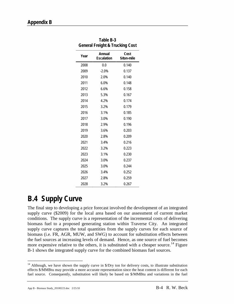
Appendix B
App B - Biomass Study_20100223.doc 2/25/10 B-4 R. W. Beck
Table B-3 General Freight & Trucking Cost
Year Annual Escalation
Cost $/ton-mile
2008 0.0 0.140 2009 -2.0% 0.137 2010 2.0% 0.140 2011 6.0% 0.148 2012 6.6% 0.158 2013 5.3% 0.167 2014 4.2% 0.174 2015 3.2% 0.179 2016 3.1% 0.185 2017 3.0% 0.190 2018 2.9% 0.196 2019 3.6% 0.203 2020 2.8% 0.209 2021 3.4% 0.216 2022 3.2% 0.223 2023 3.1% 0.230 2024 3.0% 0.237 2025 3.0% 0.244 2026 3.4% 0.252 2027 2.8% 0.259 2028 3.2% 0.267
B.4 Supply Curve The final step to developing a price forecast involved the development of an integrated supply curve ($2009) for the local area based on our assessment of current market conditions. The supply curve is a representation of the incremental costs of delivering biomass fuel to a proposed generating station within Traverse City. An integrated supply curve captures the total quantities from the supply curves for each source of biomass (i.e. FR, AGR, MUW, and SWG) to account for substitution effects between the fuel sources at increasing levels of demand. Hence, as one source of fuel becomes more expensive relative to the others, it is substituted with a cheaper source.14
14 Although, we have shown the supply curve in $/Dry ton for delivery costs, to illustrate substitution effects $/MMBtu may provide a more accurate representation since the heat content is different for each fuel source. Consequently, substitution will likely be based on $/MMBtu and variations in the fuel
Figure B-1 shows the integrated supply curve for the combined biomass fuel sources.
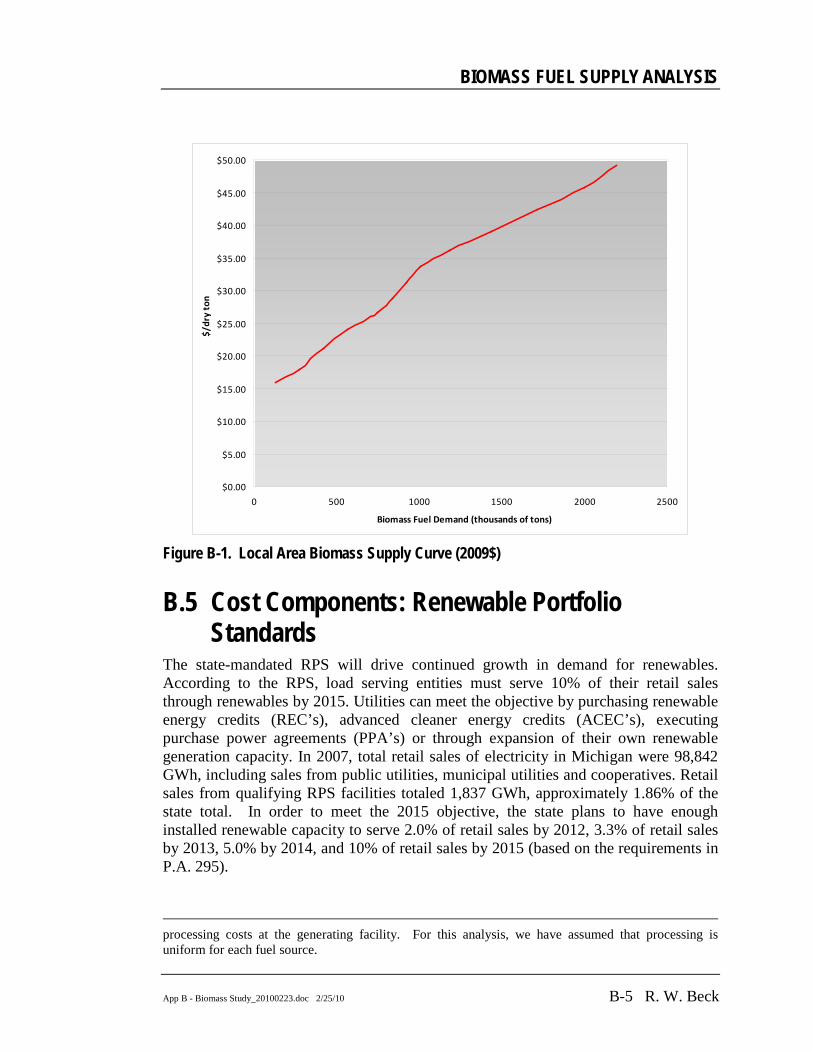
BIOMASS FUEL SUPPLY ANALYSIS
App B - Biomass Study_20100223.doc 2/25/10 B-5 R. W. Beck
$0.00
$5.00
$10.00
$15.00
$20.00
$25.00
$30.00
$35.00
$40.00
$45.00
$50.00
0 500 1000 1500 2000 2500
Biomass Fuel Demand (thousands of tons)
$/dr
y to
n
Figure B-1. Local Area Biomass Supply Curve (2009$)
B.5 Cost Components: Renewable Portfolio Standards
The state-mandated RPS will drive continued growth in demand for renewables. According to the RPS, load serving entities must serve 10% of their retail sales through renewables by 2015. Utilities can meet the objective by purchasing renewable energy credits (REC’s), advanced cleaner energy credits (ACEC’s), executing purchase power agreements (PPA’s) or through expansion of their own renewable generation capacity. In 2007, total retail sales of electricity in Michigan were 98,842 GWh, including sales from public utilities, municipal utilities and cooperatives. Retail sales from qualifying RPS facilities totaled 1,837 GWh, approximately 1.86% of the state total. In order to meet the 2015 objective, the state plans to have enough installed renewable capacity to serve 2.0% of retail sales by 2012, 3.3% of retail sales by 2013, 5.0% by 2014, and 10% of retail sales by 2015 (based on the requirements in P.A. 295).
processing costs at the generating facility. For this analysis, we have assumed that processing is uniform for each fuel source.
Appendix B
App B - Biomass Study_20100223.doc 2/25/10 B-6 R. W. Beck
Consumers Energy (CE) and Detroit Edison (DTE) serve more than 90% of the retail customers in Michigan; thus the two utilities will also drive most of the new demand for renewable resources. The service territory for CE includes most of the Lower Peninsula while DTE’s territory consists primarily of eastern Michigan. According to recent press releases and the renewable energy plans submitted by both utilities, CE and DTE plan to heavily invest in new wind projects either through acquisition of RECs, building new plants, or through executing PPAs. Specifically, DTE plans approximately $3.9 billion of expenditures to purchase renewable energy from Michigan-based facilities through 2029. The resource mix will consist primarily of wind and may also include landfill gas, biomass, solar, hydropower, and other sources approved by the Michigan Public Service Commission. CE stated that it would need 4 million MWh to meet its RPS objective. Of the 4 million MWh, 2.5 million MWh are expected to come from wind generation, and the remainder from other sources.
For the purpose of this study, we assumed that new biomass facilities would constitute no more than 10% of the RPS requirement. We also assumed that the largest utilities will distribute installation of biomass facilities throughout their service area in order to avoid transmission congestion and to not put upward price pressure on local feedstock sources.
Assumptions in model: New facilities will be distributed throughout the state based on the percentage
of statewide biomass feedstock (dry tons) available in the Local Area and by proximity to load centers.
Growth in retail load will be approximately 1.43% annually over the forecast horizon.
Transmission congestion will potentially make utilities want to distribute their generation facilities throughout the region so as not to incur costs of building new transmission and to avoid congestion.
Lack of available feedstock will force utilities to distribute generation facilities as long as there are transmission alternatives.
CE and DTE will account for most of the demand for biomass, landfill gas and wind resources.
On a state level the effect of demand for RECs and PPAs will also make development of new biomass generation facilities distributed, as developers will build where the fuel source is cheapest. Utilities will be able to purchase RECs from these facilities. For example, according to DTEs Renewable Energy Plan, 56% of their renewable portfolio will be composed of PPAs and REC and ACEC purchases.
Factors not modeled: (1) As demand increases, the proportion of biomass delivered costs due to
transportation may decrease. However, transmission congestion may affect the

BIOMASS FUEL SUPPLY ANALYSIS
App B - Biomass Study_20100223.doc 2/25/10 B-7 R. W. Beck
interconnection of facilities as new generation is more remote from the load centers. Consequently, the value of biomass feedstock in certain locations will be impacted by network constraints.
B.6 Price Forecast Results Table B-4 shows the estimated annual amount of electric generation from renewable resources that are required to meet the RPS. After 2015, additional renewable generation is still necessary, but the growth rate will follow the rate of load growth.
Table B-4 Annual Renewable Generation Requirements (MWh)15
RPS Requirement
Generation from
Renewable Resources
Generation from Biomass Resources
10% of Requirement
40% of Requirement
50% of Requirement
2009 0.0% 0 0 0 0 2010 0.0% 0 0 0 0 2011 0.0% 0 0 0 0 2012 2.0% 2,122,169 212,217 848,868 1,061,085 2013 3.3% 3,551,613 355,161 1,420,645 1,775,807 2014 5.0% 5,458,124 545,812 2,183,250 2,729,062 2015 10.0% 11,072,230 1,107,223 4,428,892 5,536,115 2016 10.0% 11,230,440 1,123,044 4,492,176 5,615,220 2017 10.0% 11,390,911 1,139,091 4,556,364 5,695,456 2018 10.0% 11,553,675 1,155,367 4,621,470 5,776,837 2019 10.0% 11,718,765 1,171,876 4,687,506 5,859,382 2020 10.0% 11,886,213 1,188,621 4,754,485 5,943,107 2021 10.0% 12,056,054 1,205,605 4,822,422 6,028,027 2022 10.0% 12,228,323 1,222,832 4,891,329 6,114,161 2023 10.0% 12,403,052 1,240,305 4,961,221 6,201,526 2024 10.0% 12,580,279 1,258,028 5,032,111 6,290,139 2025 10.0% 12,760,037 1,276,004 5,104,015 6,380,019 2026 10.0% 12,942,364 1,294,236 5,176,946 6,471,182 2027 10.0% 13,127,297 1,312,730 5,250,919 6,563,649 2028 10.0% 13,314,872 1,331,487 5,325,949 6,657,436
The delivered price of biomass fuel will be dependent on the proportion of renewable generation due to power generation from new biomass facilities. As more biomass-
15 The values listed in the table correspond to requirements. Annual electricity generation during the period 2006 through 2008 from biomass in Michigan is estimated at approximately 800,000 MWh.

Appendix B
App B - Biomass Study_20100223.doc 2/25/10 B-8 R. W. Beck
fueled power plants are installed through time and certain types of existing coal-fired plants are retro-fitted to burn the fuel, the cost of biomass fuel can be expected to increase. Table B-5 shows the projected commodity and transportation costs of biomass fuels delivered to the TCLP area assuming 10% of the projected renewable energy requirement is met with biomass resources.
Table B-5 Biomass Price Forecast At 10% of Renewable Energy Requirement Provided From
Biomass Resources
Demand Feedstock Costs Transportation Costs Biomass Price
Forecast
(Dry Tons)
(Current $/Dry Ton)
(Nominal $/Dry Ton)
(Current $/Dry Ton)
(Nominal $/Dry Ton)
(Nominal $/Dry Ton) $MMBTu*
2008 708,021 $19.08 19.08 $7.44 $7.44 $26.52 $1.57 2009 708,021 $19.08 19.54 $7.44 $7.28 $26.82 $1.59 2010 731,135 $19.35 20.29 $7.49 $7.47 $27.76 $1.64 2011 761,329 $19.87 21.34 $7.56 $8.02 $29.35 $1.74 2012 792,373 $20.64 22.69 $7.62 $8.62 $31.32 $1.85 2013 824,286 $21.43 24.13 $7.68 $9.15 $33.28 $1.97 2014 859,273 $22.30 25.71 $7.76 $9.60 $35.31 $2.09 2015 893,011 $23.13 27.31 $7.86 $10.03 $37.34 $2.21 2016 896,180 $23.21 28.06 $7.87 $10.35 $38.41 $2.27 2017 899,394 $23.29 28.83 $7.88 $10.70 $39.53 $2.34 2018 902,655 $23.37 29.62 $7.89 $11.06 $40.68 $2.41 2019 905,962 $23.45 30.44 $7.90 $11.42 $41.86 $2.48 2020 909,316 $23.54 31.29 $7.91 $11.81 $43.10 $2.55 2021 912,718 $23.62 32.15 $7.92 $12.20 $44.35 $2.62 2022 916,169 $23.71 33.05 $7.93 $12.60 $45.65 $2.70 2023 919,669 $23.79 33.95 $7.94 $13.02 $46.98 $2.78 2024 923,219 $23.88 34.90 $7.95 $13.46 $48.36 $2.86 2025 926,820 $23.97 35.87 $7.96 $13.90 $49.78 $2.94 2026 930,472 $24.06 36.87 $7.97 $14.37 $51.24 $3.03 2027 934,176 $24.15 37.90 $7.98 $14.85 $52.74 $3.12 2028 937,934 $24.25 38.97 $7.99 $15.34 $54.31 $3.21 * Conversion from $/Dry Ton to $/MMBtu assumes heat content of approximately 8,500 Btu/lb.

Appendix C STOCHASTIC ECONOMETRIC REGIONAL
FORECASTING MODEL


App C - Stochastic Eon Reg Forecasting Model.doc 2/25/10 R. W. Beck C-1
Appendix C STOCHASTIC ECONOMETRIC
REGIONAL FORECASTING MODEL
C.1 Overview of Model For the IRP Study, the R. W. Beck proprietary Stochastic Econometric Regional Forecasting (“SERF”) model was used. The SERF model generates stochastic projections of fuel prices, electric loads for the region and the subject utility (in this case TCLP), emission prices, and power prices. The model simulates corresponding utility power supply costs for multiple potential resource expansion portfolios based on the stochastic projections. A stochastic dynamic programming algorithm determines the optimal resource expansion decisions. The general structure of the SERF model is depicted below in Figure 5-1.
SERF consists of three primary modules:
Stochastic Market Module, which generates stochastic projections of fuel, power prices, utility loads, and emission prices and simulates the build-out and commitment/dispatch of market resources;
Production Cost Module, which simulates a utility’s generating resource commitment and dispatch; and
Stochastic–Dynamic Optimization Module, which determines a utility’s optimal generation expansion plan given uncertain load and market and commodity price conditions.
LoadForecast
LoadForecast
FuelPrice Forecast
FuelPrice Forecast
TransmissionSystem Analysis
TransmissionSystem Analysis
Existing Resource
Characteristics
Existing Resource
CharacteristicsNew Resource
OptionsNew Resource
Options
Develop Regional Load, Market and Fuel Price Scenarios (Draws)
Develop Regional Load, Market and Fuel Price Scenarios (Draws)
Simulation of Potential Power Supply PortfoliosUnder Scenarios (Draws) of Prices and Load
Simulation of Potential Power Supply PortfoliosUnder Scenarios (Draws) of Prices and Load
Identify Least-Cost / Risk Plan(s) and Develop Resource Selection RulesIdentify Least-Cost / Risk Plan(s) and Develop Resource Selection Rules
STOCHASTIC MARKET MODULE
PARAMETERS
PORTFOLIO DEVELOPMENT MODULE
PRODUCTION COST MODULE
STOCHASTIC-DYNAMIC OPTIMIZATION MODULE
Construct Portfolios ofPossible Resource Options
Construct Portfolios ofPossible Resource Options
Figure C-1: SERF Model Overview
The discussion in the following sections describes each of the modules.
Appendix C
App C - Stochastic Eon Reg Forecasting Model.doc 2/25/10 C-2 R. W. Beck
C.1.1 Stochastic Market Module The Stochastic Market Module was used to simulate market conditions and power prices for the MISO East and surrounding market regions. The Stochastic Market Module works in the following manner.
Step 1: For a given number random paths of future uncertain conditions, for each simulated region, and for each year of the study period, the module generates stochastic projections of hourly loads, daily gas prices, monthly coal prices, and hourly hydroelectric generation. The stochastic projections reflect several important correlations, including those among fuels, those for load across the simulated regions, and those for load between the regions and the subject utility.
Step 2: For each random path and hour, a multi-area dispatch algorithm is used to calculate the marginal cost of power in each region. This algorithm dispatches available generating capacity to meet the load projected in Step 1 in all modeled regions at the lowest possible cost, taking into account fuel prices and hydroelectric generation projected in Step 1, and the operating characteristics of the available capacity (e.g., capacity rating, heat rate, variable O&M cost, emissions costs).
Step 3: Stochastic equations relating the power price to the marginal cost are used to generate projections of hourly electric prices for each random path, hour, and region, using the marginal cost projections from Step 3.
Step 4: For the initial years of the study period, and for all paths, the capacity available for dispatch in Step 2 is comprised of the existing fleet of plants, less planned retirements, plus planned additions. Thereafter, the available capacity varies across paths, and is determined in the following manner.
In processing each random path, the module considers at the beginning of each year the possible capacity additions for the path multiple years into the future (reflecting generation expansion decisions that must be made prior to the date of actual need). The module then simulates a given number of secondary random paths of regional loads, fuel prices, hydroelectric generation, marginal power costs, and power prices prior to the on-line date of potential new resources to simulate potential resource decisions given the level of uncertainty that exists at the time the resource expansion decision must be made.
The algorithm calculates the market value from the secondary draws as of the on-line date for each potential generating resource alternative. If one or more of the alternatives has positive expected profits, the algorithm builds the resource and adds it to the regional market stack for that primary path. The algorithm iterates until planning reserve requirements are met and no more profitable resource additions can be made.
Once the algorithm has determined the capacity additions for the primary path for a particular future year, the module simulates loads and prices for the path for the decision year and then repeats the capacity expansion decision process
STOCHASTIC ECONOMETRIC REGIONAL FORECASTING MODEL
App C - Stochastic Eon Reg Forecasting Model.doc 2/25/10 R. W. Beck C-3
for each subsequent year for each primary random path until the end of the study period is reached.
Through this process, the algorithm constructs a generation expansion plan for each primary path by simulating resource expansion decisions prior to the actual on-line dates of potential resources given uncertain market conditions (i.e., simulating real world decision-making processes).
The equations used to generate projections of loads, fuel prices, hydroelectric generation, and power prices are stochastic in nature and include both (i) parameters that describe the expected evolution of the variable over time and (ii) parameters that describe the volatility of the variable over time. The parameters of these equations are estimated econometrically, using available historical data.
The equations for loads, fuel prices, and hydroelectric generation are all univariate. In other words, the expected value of a variable depends on the previous values of the variable, time, and random disturbances, but not the values of the other variables. For loads, the process for simulating hourly values is processed as three separate but linked stages: an equation for annual loads, an equation for monthly loads (conditional on the annual load), and an equation for hourly loads (conditional on the monthly loads). Similarly, the equations for daily natural gas prices is modeled as separate (but linked) annual, monthly, and daily equations; and the monthly equations for coal prices, as linked annual and monthly equations. For loads and fuel prices, monthly, daily, and hourly volatilities are treated as time varying, with a Generalized Autoregressive Conditional Heteroskedasticity (GARCH) structure.
C.1.2 Production Cost Module
The expected power price and its volatility in a market region and hour is a function of the simulated marginal cost in the region by hour and the relationship of load to capacity in the region. The parameters of these equations are estimated by simulating historical marginal costs or market prices from the multi-region dispatch algorithm, and econometrically analyzing the resulting simulated costs together with actual price, load, and capacity data.
Resources are committed and dispatched as required to serve load and initiate sale of power to the market at the projected hourly power prices developed by the Stochastic Market Module, taking into account projected monthly/daily fuel prices and the operating characteristics of the generating units in a portfolio (e.g., capacity ratings, minimum up and down times, startup costs, non-linear heat-rate curves, etc.). The algorithm determines the amount of power to generate for load and sell in each hour (up to user-specified quantity limits) by determining the output that would minimize net production costs for the year.
The Production Cost Module is a standard market-based chronological commitment and dispatch algorithm. For each random path and potential portfolio of resource alternatives, the algorithm works in the following manner.
Appendix C
App C - Stochastic Eon Reg Forecasting Model.doc 2/25/10 C-4 R. W. Beck
Power can be purchased from the market to satisfy the utility’s projected hourly loads at the projected hourly power prices when such purchases are lower costs that self-generation (and within user-specified quantity limits).
The total net production cost for each random path, year, and portfolio is computed as the sum of costs of generation and market purchases, less market sales revenue.
C.1.3 Stochastic Dynamic Optimization Module The Stochastic Dynamic Optimization Module works in the following manner.
For the purpose of making investment decisions, three variables are considered to be stochastic: the utility’s annual average load, the average annual natural gas price, and the average annual market-implied heat rate (i.e., the average power price divided by the average natural gas price). For each year of the study period, the probability distribution of each of these four variables is determined, and the value of each variable at user-defined percentiles (e.g., 10th, 30th, 50th, 70th, and 90th) is calculated. Each possible combination of the three stochastic variables and percentiles is referred to as an “Evaluation Point.”
The algorithm works backward through time (starting at the end of the study period), evaluating the best capacity expansion decisions that can be made for a future year (i.e., the decision must be made prior to the on-line date). The algorithm makes a separate decision for (i) each of the possible Evaluation Points and (ii) each possible prior year investment decision.
In each year, the algorithm performs the following steps:
– For each Evaluation Point, the algorithm calculates the expected value of each of the three stochastic variables in the installation year, as well the variance of each variable. For each possible portfolio in the installation year, the algorithm combines these expected values and variances with the results from the Production Cost Module to calculate the expected value and variance of annual production costs and fixed costs for the portfolio.
– For each Evaluation Point and potential prior year decisions, the algorithm identifies the portfolios that best satisfies the decision criterion and is feasible (satisfies utility-specific planning requirements and represents a possible portfolio given subsequent year decisions). At each decision point, the algorithm can use either of two decision criteria: select the portfolio with the lowest expected value of future total system costs or select the portfolio with the lowest risk, or exposure.
Continuing to move backward through time, the algorithm addresses the decisions to be made in prior years in much the same manner, but also giving consideration to the set of possible portfolios for a given random path that contain resource alternatives that were already identified as least cost alternatives in later years of the study. This process continues until the first year

STOCHASTIC ECONOMETRIC REGIONAL FORECASTING MODEL
App C - Stochastic Eon Reg Forecasting Model.doc 2/25/10 R. W. Beck C-5
of the study period is reached and the lowest-cost or least risk plan can be readily identified.


Appendix D POWER SUPPLY PLAN RESULTS


Table D1.1 Traverse City Light & Power
Resource Plan - AnnualExisting Resources
2010 2011 2012 2013 2014 2015 2016 2017 2018 2019
Peak Demand (MW)Peak Demand 74.9 75.1 74.9 75.5 77.2 77.5 77.5 78.3 78.7 79.1 Reserves 11.2 11.3 11.2 11.3 11.6 11.6 11.6 11.7 11.8 11.9
Capacity Requirements 86.1 86.4 86.1 86.8 88.8 89.2 89.1 90.0 90.5 90.9
Capacity Resources (MW)Existing Resources
Belle River 10.4 10.4 10.4 10.4 10.4 10.4 10.4 10.4 10.4 10.4 Campbell 3 10.5 10.5 10.5 10.5 10.5 10.5 10.5 10.5 10.5 10.5 Kalkaska CT 36.9 36.9 36.9 36.9 36.9 36.9 36.9 36.9 36.9 36.9 Existing Wind* 0.05 0.05 0.05 0.05 0.05 0.05 0.05 0.05 0.05 0.05 Granger Landfill Gas 0.3 0.8 0.9 1.4 1.4 1.7 1.7 1.7 1.7 1.7 Total 58.1 58.6 58.7 59.3 59.3 59.5 59.5 59.5 59.5 59.5
Future ResourcesSCP Coal wCCS - - - - - - - - - - Combined Cycle - - - - - - - - - - Combustion Turbine - - - - - - - - - - Heritage Wind* - 0.8 0.8 0.8 0.8 0.8 0.8 0.8 0.8 0.8 New Solar - - - - - - - - - - TCLP Biomass - - - - - - - - - - Market Purchases 28.1 27.0 26.6 26.8 28.7 28.9 28.8 29.7 30.2 30.6 Total 28.1 27.8 27.4 27.6 29.5 29.7 29.6 30.5 31.0 31.4
Total Capacity 86.1 86.4 86.1 86.8 88.8 89.2 89.1 90.0 90.5 90.9 Surplus/(Deficiency) - - - - - - - - - -
Energy from Renewable Resources 0.9% 8.1% 8.5% 9.7% 9.4% 10.0% 9.9% 9.8% 9.8% 9.7%State REP Requirement 0.0% 0.0% 2.0% 3.3% 5.0% 10.0% 9.9% 9.9% 9.8% 9.7%TCLP RPS Goal 0.0% 0.0% 2.0% 3.3% 5.0% 10.0% 10.0% 10.0% 10.0% 10.0%
R:\Orlando\010633 - Traverse City\05-01528-20101 IRP\Data-Analytical\SERF Results\TCLP Results - Working_V17.xlsb Page 1 of 8 R. W. Beck, Inc. 2/25/2010
_______________ * Reflects a capacity credit for resource adequacy purposes of 8% of nameplate capacity per the currently proposed MISO default standard.
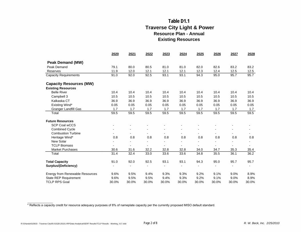
Peak Demand (MW)Peak DemandReserves
Capacity Requirements
Capacity Resources (MW)Existing Resources
Belle RiverCampbell 3Kalkaska CTExisting Wind*Granger Landfill GasTotal
Future ResourcesSCP Coal wCCSCombined CycleCombustion TurbineHeritage Wind*New SolarTCLP BiomassMarket PurchasesTotal
Total CapacitySurplus/(Deficiency)
Energy from Renewable ResourcesState REP RequirementTCLP RPS Goal
Table D1.1 Traverse City Light & Power
Resource Plan - AnnualExisting Resources
2020 2021 2022 2023 2024 2025 2026 2027 2028
79.1 80.0 80.5 81.0 81.0 82.0 82.6 83.2 83.2 11.9 12.0 12.1 12.1 12.1 12.3 12.4 12.5 12.5 91.0 92.0 92.5 93.1 93.1 94.3 95.0 95.7 95.7
10.4 10.4 10.4 10.4 10.4 10.4 10.4 10.4 10.4 10.5 10.5 10.5 10.5 10.5 10.5 10.5 10.5 10.5 36.9 36.9 36.9 36.9 36.9 36.9 36.9 36.9 36.9 0.05 0.05 0.05 0.05 0.05 0.05 0.05 0.05 0.05 1.7 1.7 1.7 1.7 1.7 1.7 1.7 1.7 1.7
59.5 59.5 59.5 59.5 59.5 59.5 59.5 59.5 59.5
- - - - - - - - - - - - - - - - - - - - - - - - - - - 0.8 0.8 0.8 0.8 0.8 0.8 0.8 0.8 0.8 - - - - - - - - - - - - - - - - - -
30.6 31.6 32.2 32.8 32.8 34.0 34.7 35.3 35.4 31.4 32.4 33.0 33.6 33.6 34.8 35.5 36.1 36.2
91.0 92.0 92.5 93.1 93.1 94.3 95.0 95.7 95.7 - - - - - - - - -
9.6% 9.5% 9.4% 9.3% 9.3% 9.2% 9.1% 9.0% 8.9%9.6% 9.5% 9.5% 9.4% 9.3% 9.2% 9.1% 9.0% 8.9%
30.0% 30.0% 30.0% 30.0% 30.0% 30.0% 30.0% 30.0% 30.0%
R:\Orlando\010633 - Traverse City\05-01528-20101 IRP\Data-Analytical\SERF Results\TCLP Results - Working_V17.xlsb Page 2 of 8 R. W. Beck, Inc. 2/25/2010
_______________ * Reflects a capacity credit for resource adequacy purposes of 8% of nameplate capacity per the currently proposed MISO default standard.

Table D1.2 Traverse City Light & Power
Resource Plan - AnnualOptimal Plan - Case 1
2010 2011 2012 2013 2014 2015 2016 2017 2018 2019
Peak Demand (MW)Peak Demand 74.9 75.1 74.9 75.5 77.2 77.5 77.5 78.3 78.7 79.1 Reserves 11.2 11.3 11.2 11.3 11.6 11.6 11.6 11.7 11.8 11.9
Capacity Requirements 86.1 86.4 86.1 86.8 88.8 89.2 89.1 90.0 90.5 90.9
Capacity Resources (MW)Existing Resources
Belle River 10.4 10.4 10.4 10.4 10.4 10.4 10.4 10.4 10.4 10.4 Campbell 3 10.5 10.5 10.5 10.5 10.5 10.5 10.5 10.5 10.5 10.5 Kalkaska CT 36.9 36.9 36.9 36.9 36.9 36.9 36.9 36.9 36.9 36.9 Existing Wind* 0.05 0.05 0.05 0.05 0.05 0.05 0.05 0.05 0.05 0.05 Granger Landfill Gas 0.3 0.8 0.9 1.4 1.4 1.7 1.7 1.7 1.7 1.7 Total 58.1 58.6 58.7 59.3 59.3 59.5 59.5 59.5 59.5 59.5
Future ResourcesSCP Coal wCCS - - - - - - - - - - Combined Cycle - - - - - - - - - - Combustion Turbine - - - - - 12.5 12.5 12.5 12.5 12.5 Heritage Wind* - 0.8 0.8 0.8 0.8 0.8 0.8 0.8 0.8 0.8 New Solar - - - - - - - - - - TCLP Biomass - - - - - 10.0 10.0 10.0 10.0 10.0 Market Purchases 28.1 27.0 26.6 26.8 28.7 6.3 6.3 7.2 7.7 8.1 Total 28.1 27.8 27.4 27.6 29.5 29.7 29.6 30.5 31.0 31.4
Total Capacity 86.1 86.4 86.1 86.8 88.8 89.2 89.1 90.0 90.5 90.9 Surplus/(Deficiency) - - - - - - - - - -
Energy from Renewable Resources 0.9% 8.1% 8.5% 9.7% 9.4% 29.1% 28.8% 28.5% 28.0% 27.8%State REP Requirement 0.0% 0.0% 2.0% 3.3% 5.0% 10.0% 9.9% 9.9% 9.8% 9.7%TCLP RPS Goal 0.0% 0.0% 2.0% 3.3% 5.0% 10.0% 10.0% 10.0% 10.0% 10.0%
R:\Orlando\010633 - Traverse City\05-01528-20101 IRP\Data-Analytical\SERF Results\TCLP Results - Working_V17.xlsb Page 3 of 8 R. W. Beck, Inc. 2/25/2010
_______________ * Reflects a capacity credit for resource adequacy purposes of 8% of nameplate capacity per the currently proposed MISO default standard.

Peak Demand (MW)Peak DemandReserves
Capacity Requirements
Capacity Resources (MW)Existing Resources
Belle RiverCampbell 3Kalkaska CTExisting Wind*Granger Landfill GasTotal
Future ResourcesSCP Coal wCCSCombined CycleCombustion TurbineHeritage Wind*New SolarTCLP BiomassMarket PurchasesTotal
Total CapacitySurplus/(Deficiency)
Energy from Renewable ResourcesState REP RequirementTCLP RPS Goal
Table D1.2 Traverse City Light & Power
Resource Plan - AnnualOptimal Plan - Case 1
2020 2021 2022 2023 2024 2025 2026 2027 2028
79.1 80.0 80.5 81.0 81.0 82.0 82.6 83.2 83.2 11.9 12.0 12.1 12.1 12.1 12.3 12.4 12.5 12.5 91.0 92.0 92.5 93.1 93.1 94.3 95.0 95.7 95.7
10.4 10.4 10.4 10.4 10.4 10.4 10.4 10.4 10.4 10.5 10.5 10.5 10.5 10.5 10.5 10.5 10.5 10.5 36.9 36.9 36.9 36.9 36.9 36.9 36.9 36.9 36.9 0.05 0.05 0.05 0.05 0.05 0.05 0.05 0.05 0.05 1.7 1.7 1.7 1.7 1.7 1.7 1.7 1.7 1.7
59.5 59.5 59.5 59.5 59.5 59.5 59.5 59.5 59.5
- - - - - - - - - - - - - - - - - -
12.5 12.5 12.5 12.5 12.5 12.5 12.5 12.5 12.5 0.8 0.8 0.8 0.8 0.8 0.8 0.8 0.8 0.8 - - - - - - - - -
10.0 10.0 10.0 10.0 10.0 10.0 10.0 10.0 10.0 8.1 9.1 9.7 10.3 10.3 11.5 12.2 12.8 12.9
31.4 32.4 33.0 33.6 33.6 34.8 35.5 36.1 36.2
91.0 92.0 92.5 93.1 93.1 94.3 95.0 95.7 95.7 - - - - - - - - -
27.0% 27.0% 26.6% 26.3% 26.3% 26.0% 25.8% 25.5% 25.4%9.6% 9.5% 9.5% 9.4% 9.3% 9.2% 9.1% 9.0% 8.9%
30.0% 30.0% 30.0% 30.0% 30.0% 30.0% 30.0% 30.0% 30.0%
R:\Orlando\010633 - Traverse City\05-01528-20101 IRP\Data-Analytical\SERF Results\TCLP Results - Working_V17.xlsb Page 4 of 8 R. W. Beck, Inc. 2/25/2010
_______________ * Reflects a capacity credit for resource adequacy purposes of 8% of nameplate capacity per the currently proposed MISO default standard.

Table D1.3 Traverse City Light & Power
Resource Plan - AnnualOptimal Plan - Case 2
2010 2011 2012 2013 2014 2015 2016 2017 2018 2019
Peak Demand (MW)Peak Demand 74.9 75.1 74.9 75.5 77.2 77.5 77.5 78.3 78.7 79.1 Reserves 11.2 11.3 11.2 11.3 11.6 11.6 11.6 11.7 11.8 11.9
Capacity Requirements 86.1 86.4 86.1 86.8 88.8 89.2 89.1 90.0 90.5 90.9
Capacity Resources (MW)Existing Resources
Belle River 10.4 10.4 10.4 10.4 10.4 10.4 10.4 10.4 10.4 10.4 Campbell 3 10.5 10.5 10.5 10.5 10.5 10.5 10.5 10.5 10.5 10.5 Kalkaska CT 36.9 36.9 36.9 36.9 36.9 36.9 36.9 36.9 36.9 36.9 Existing Wind* 0.05 0.05 0.05 0.05 0.05 0.05 0.05 0.05 0.05 0.05 Granger Landfill Gas 0.3 0.8 0.9 1.4 1.4 1.7 1.7 1.7 1.7 1.7 Total 58.1 58.6 58.7 59.3 59.3 59.5 59.5 59.5 59.5 59.5
Future ResourcesSCP Coal wCCS - - - - - - - - - - Combined Cycle - - - - - - - - - - Combustion Turbine - - - - - 6.3 6.3 6.3 6.3 6.3 Heritage Wind* - 0.8 0.8 0.8 0.8 0.8 0.8 0.8 0.8 0.8 New Solar - - - - - - - - - - TCLP Biomass - - - - - 20.0 20.0 20.0 20.0 20.0 Market Purchases 28.1 27.0 26.6 26.8 28.7 2.6 2.6 3.4 3.9 4.3 Total 28.1 27.8 27.4 27.6 29.5 29.7 29.6 30.5 31.0 31.4
Total Capacity 86.1 86.4 86.1 86.8 88.8 89.2 89.1 90.0 90.5 90.9 Surplus/(Deficiency) - - - - - - - - - -
Energy from Renewable Resources 0.9% 8.1% 8.5% 9.7% 9.4% 48.2% 47.6% 47.1% 46.2% 45.9%State REP Requirement 0.0% 0.0% 2.0% 3.3% 5.0% 10.0% 9.9% 9.9% 9.8% 9.7%TCLP RPS Goal 0.0% 0.0% 2.0% 3.3% 5.0% 10.0% 10.0% 10.0% 10.0% 10.0%
R:\Orlando\010633 - Traverse City\05-01528-20101 IRP\Data-Analytical\SERF Results\TCLP Results - Working_V17.xlsb Page 5 of 8 R. W. Beck, Inc. 2/25/2010
_______________ * Reflects a capacity credit for resource adequacy purposes of 8% of nameplate capacity per the currently proposed MISO default standard.

Peak Demand (MW)Peak DemandReserves
Capacity Requirements
Capacity Resources (MW)Existing Resources
Belle RiverCampbell 3Kalkaska CTExisting Wind*Granger Landfill GasTotal
Future ResourcesSCP Coal wCCSCombined CycleCombustion TurbineHeritage Wind*New SolarTCLP BiomassMarket PurchasesTotal
Total CapacitySurplus/(Deficiency)
Energy from Renewable ResourcesState REP RequirementTCLP RPS Goal
Table D1.3 Traverse City Light & Power
Resource Plan - AnnualOptimal Plan - Case 2
2020 2021 2022 2023 2024 2025 2026 2027 2028
79.1 80.0 80.5 81.0 81.0 82.0 82.6 83.2 83.2 11.9 12.0 12.1 12.1 12.1 12.3 12.4 12.5 12.5 91.0 92.0 92.5 93.1 93.1 94.3 95.0 95.7 95.7
10.4 10.4 10.4 10.4 10.4 10.4 10.4 10.4 10.4 10.5 10.5 10.5 10.5 10.5 10.5 10.5 10.5 10.5 36.9 36.9 36.9 36.9 36.9 36.9 36.9 36.9 36.9 0.05 0.05 0.05 0.05 0.05 0.05 0.05 0.05 0.05 1.7 1.7 1.7 1.7 1.7 1.7 1.7 1.7 1.7
59.5 59.5 59.5 59.5 59.5 59.5 59.5 59.5 59.5
- - - - - - - - - - - - - - - - - - 6.3 6.3 6.3 6.3 6.3 6.3 6.3 6.3 6.3 0.8 0.8 0.8 0.8 0.8 0.8 0.8 0.8 0.8 - - - - - - - - -
20.0 20.0 20.0 20.0 20.0 20.0 20.0 20.0 20.0 4.4 5.4 6.0 6.5 6.6 7.7 8.4 9.1 9.2
31.4 32.4 33.0 33.6 33.6 34.8 35.5 36.1 36.2
91.0 92.0 92.5 93.1 93.1 94.3 95.0 95.7 95.7 - - - - - - - - -
44.4% 44.6% 43.9% 43.3% 43.3% 42.9% 42.5% 42.1% 41.9%9.6% 9.5% 9.5% 9.4% 9.3% 9.2% 9.1% 9.0% 8.9%
30.0% 30.0% 30.0% 30.0% 30.0% 30.0% 30.0% 30.0% 30.0%
R:\Orlando\010633 - Traverse City\05-01528-20101 IRP\Data-Analytical\SERF Results\TCLP Results - Working_V17.xlsb Page 6 of 8 R. W. Beck, Inc. 2/25/2010
_______________ * Reflects a capacity credit for resource adequacy purposes of 8% of nameplate capacity per the currently proposed MISO default standard.
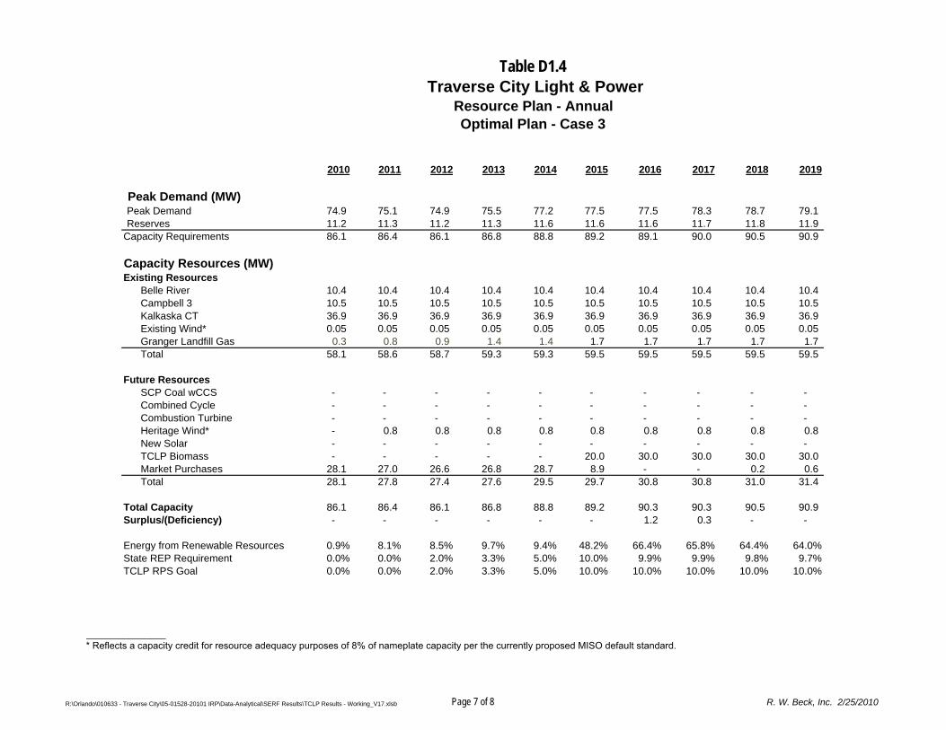
Table D1.4 Traverse City Light & Power
Resource Plan - AnnualOptimal Plan - Case 3
2010 2011 2012 2013 2014 2015 2016 2017 2018 2019
Peak Demand (MW)Peak Demand 74.9 75.1 74.9 75.5 77.2 77.5 77.5 78.3 78.7 79.1 Reserves 11.2 11.3 11.2 11.3 11.6 11.6 11.6 11.7 11.8 11.9
Capacity Requirements 86.1 86.4 86.1 86.8 88.8 89.2 89.1 90.0 90.5 90.9
Capacity Resources (MW)Existing Resources
Belle River 10.4 10.4 10.4 10.4 10.4 10.4 10.4 10.4 10.4 10.4 Campbell 3 10.5 10.5 10.5 10.5 10.5 10.5 10.5 10.5 10.5 10.5 Kalkaska CT 36.9 36.9 36.9 36.9 36.9 36.9 36.9 36.9 36.9 36.9 Existing Wind* 0.05 0.05 0.05 0.05 0.05 0.05 0.05 0.05 0.05 0.05 Granger Landfill Gas 0.3 0.8 0.9 1.4 1.4 1.7 1.7 1.7 1.7 1.7 Total 58.1 58.6 58.7 59.3 59.3 59.5 59.5 59.5 59.5 59.5
Future ResourcesSCP Coal wCCS - - - - - - - - - - Combined Cycle - - - - - - - - - - Combustion Turbine - - - - - - - - - - Heritage Wind* - 0.8 0.8 0.8 0.8 0.8 0.8 0.8 0.8 0.8 New Solar - - - - - - - - - - TCLP Biomass - - - - - 20.0 30.0 30.0 30.0 30.0 Market Purchases 28.1 27.0 26.6 26.8 28.7 8.9 - - 0.2 0.6 Total 28.1 27.8 27.4 27.6 29.5 29.7 30.8 30.8 31.0 31.4
Total Capacity 86.1 86.4 86.1 86.8 88.8 89.2 90.3 90.3 90.5 90.9 Surplus/(Deficiency) - - - - - - 1.2 0.3 - -
Energy from Renewable Resources 0.9% 8.1% 8.5% 9.7% 9.4% 48.2% 66.4% 65.8% 64.4% 64.0%State REP Requirement 0.0% 0.0% 2.0% 3.3% 5.0% 10.0% 9.9% 9.9% 9.8% 9.7%TCLP RPS Goal 0.0% 0.0% 2.0% 3.3% 5.0% 10.0% 10.0% 10.0% 10.0% 10.0%
R:\Orlando\010633 - Traverse City\05-01528-20101 IRP\Data-Analytical\SERF Results\TCLP Results - Working_V17.xlsb Page 7 of 8 R. W. Beck, Inc. 2/25/2010
_______________ * Reflects a capacity credit for resource adequacy purposes of 8% of nameplate capacity per the currently proposed MISO default standard.

Peak Demand (MW)Peak DemandReserves
Capacity Requirements
Capacity Resources (MW)Existing Resources
Belle RiverCampbell 3Kalkaska CTExisting Wind*Granger Landfill GasTotal
Future ResourcesSCP Coal wCCSCombined CycleCombustion TurbineHeritage Wind*New SolarTCLP BiomassMarket PurchasesTotal
Total CapacitySurplus/(Deficiency)
Energy from Renewable ResourcesState REP RequirementTCLP RPS Goal
Table D1.4 Traverse City Light & Power
Resource Plan - AnnualOptimal Plan - Case 3
2020 2021 2022 2023 2024 2025 2026 2027 2028
79.1 80.0 80.5 81.0 81.0 82.0 82.6 83.2 83.2 11.9 12.0 12.1 12.1 12.1 12.3 12.4 12.5 12.5 91.0 92.0 92.5 93.1 93.1 94.3 95.0 95.7 95.7
10.4 10.4 10.4 10.4 10.4 10.4 10.4 10.4 10.4 10.5 10.5 10.5 10.5 10.5 10.5 10.5 10.5 10.5 36.9 36.9 36.9 36.9 36.9 36.9 36.9 36.9 36.9 0.05 0.05 0.05 0.05 0.05 0.05 0.05 0.05 0.05 1.7 1.7 1.7 1.7 1.7 1.7 1.7 1.7 1.7
59.5 59.5 59.5 59.5 59.5 59.5 59.5 59.5 59.5
- - - - - - - - - - - - - - - - - - - - - - - - - - - 0.8 0.8 0.8 0.8 0.8 0.8 0.8 0.8 0.8 - - - - - - - - -
30.0 30.0 30.0 30.0 30.0 30.0 30.0 30.0 30.0 0.6 1.6 2.2 2.8 2.8 4.0 4.7 5.3 5.4
31.4 32.4 33.0 33.6 33.6 34.8 35.5 36.1 36.2
91.0 92.0 92.5 93.1 93.1 94.3 95.0 95.7 95.7 - - - - - - - - -
61.9% 62.1% 61.1% 60.2% 60.3% 59.7% 59.3% 58.6% 58.4%9.6% 9.5% 9.5% 9.4% 9.3% 9.2% 9.1% 9.0% 8.9%
30.0% 30.0% 30.0% 30.0% 30.0% 30.0% 30.0% 30.0% 30.0%
R:\Orlando\010633 - Traverse City\05-01528-20101 IRP\Data-Analytical\SERF Results\TCLP Results - Working_V17.xlsb Page 8 of 8 R. W. Beck, Inc. 2/25/2010
_______________ * Reflects a capacity credit for resource adequacy purposes of 8% of nameplate capacity per the currently proposed MISO default standard.

Table D2.1 Traverse City Light & Power
Power Supply Costs of Resource PlanExisting Resources
2010 2011 2012 2013 2014 2015 2016 2017 2018 2019 20201 1 1 1 1 1 1 1 1 1 1
Net Production Costs [1] 19,182,895$ 21,619,643$ 26,754,582$ 27,837,405$ 29,138,525$ 30,827,049$ 31,345,197$ 32,302,940$ 33,866,377$ 36,010,406$ 36,996,695$ Existing Debt Service Cost 3,688,000$ 3,692,000$ 3,687,000$ 3,672,000$ 3,629,000$ 3,590,000$ 2,872,000$ 2,872,000$ 2,153,000$ 1,817,000$ 1,817,000$ Other Debt Service Cost -$ -$ -$ -$ -$ -$ -$ -$ -$ -$ -$ Debt Service Cost of New Resources -$ -$ -$ -$ -$ -$ -$ -$ -$ -$ -$ Transmission Costs -$ -$ -$ -$ -$ -$ -$ -$ -$ -$ -$ Total Power Costs 22,870,895$ 25,311,643$ 30,441,582$ 31,509,405$ 32,767,525$ 34,417,049$ 34,217,197$ 35,174,940$ 36,019,377$ 37,827,406$ 38,813,695$ Energy (MWh) 349,844 351,857 353,027 355,531 364,545 366,828 369,963 371,787 375,291 378,214 381,071
Total Power Costs ($/MWh) 65.37$ 71.94$ 86.23$ 88.63$ 89.89$ 93.82$ 92.49$ 94.61$ 95.98$ 100.02$ 101.85$ Levelized Power Costs ($/MWh) 102.87$
Standard Deviation ($/MWh) 12.60$
5th Percentile ($/MWh) 57.22$ 63.16$ 76.01$ 75.76$ 76.83$ 75.11$ 74.08$ 77.19$ 74.44$ 79.26$ 80.34$
95th Percentile ($/MWh) 72.93$ 80.97$ 99.43$ 101.94$ 105.11$ 111.88$ 109.29$ 111.83$ 115.36$ 125.46$ 126.52$
Table D2.2 Traverse City Light & Power
Power Supply Costs of Resource PlanOptimal Plan - Case 1
2010 2011 2012 2013 2014 2015 2016 2017 2018 2019 20201 1 1 1 1 14 14 14 14 14 14
Net Production Costs [1] 19,182,895$ 21,619,643$ 26,754,582$ 27,837,405$ 29,138,525$ 24,815,462$ 25,595,329$ 26,679,539$ 28,300,587$ 30,143,512$ 31,370,559$ Existing Debt Service Cost 3,688,000$ 3,692,000$ 3,687,000$ 3,672,000$ 3,629,000$ 3,590,000$ 2,872,000$ 2,872,000$ 2,153,000$ 1,817,000$ 1,817,000$ Other Debt Service Cost -$ -$ -$ -$ -$ -$ -$ -$ -$ -$ -$ Debt Service Cost of New Resources -$ -$ -$ -$ -$ 4,704,155$ 4,704,155$ 4,704,155$ 4,704,155$ 4,704,155$ 4,704,155$ Transmission Costs -$ -$ -$ -$ -$ -$ -$ -$ -$ -$ -$ Total Power Costs 22,870,895$ 25,311,643$ 30,441,582$ 31,509,405$ 32,767,525$ 33,109,617$ 33,171,484$ 34,255,694$ 35,157,742$ 36,664,667$ 37,891,714$ Energy (MWh) 349,844 351,857 353,027 355,531 364,545 366,828 369,963 371,787 375,291 378,214 381,071
Total Power Costs ($/MWh) 65.37$ 71.94$ 86.23$ 88.63$ 89.89$ 90.26$ 89.66$ 92.14$ 93.68$ 96.94$ 99.43$ Levelized Power Costs ($/MWh) 99.97$
Standard Deviation ($/MWh) 10.93$
5th Percentile ($/MWh) 57.22$ 63.16$ 76.01$ 75.76$ 76.83$ 76.35$ 76.40$ 76.85$ 76.86$ 78.21$ 82.12$
95th Percentile ($/MWh) 72.93$ 80.97$ 99.43$ 101.94$ 105.11$ 105.79$ 104.51$ 106.28$ 110.79$ 116.32$ 119.38$
R:\Orlando\010633 - Traverse City\05-01528-20101 IRP\Data-Analytical\SERF Results\TCLP Results - Working_V17.xlsb Page 1 of 4 R. W. Beck, Inc.; 2/25/2010
_____________________ [1] Includes fuel costs, fixed and variable operation and maintenance costs, and environmental costs of all resources.
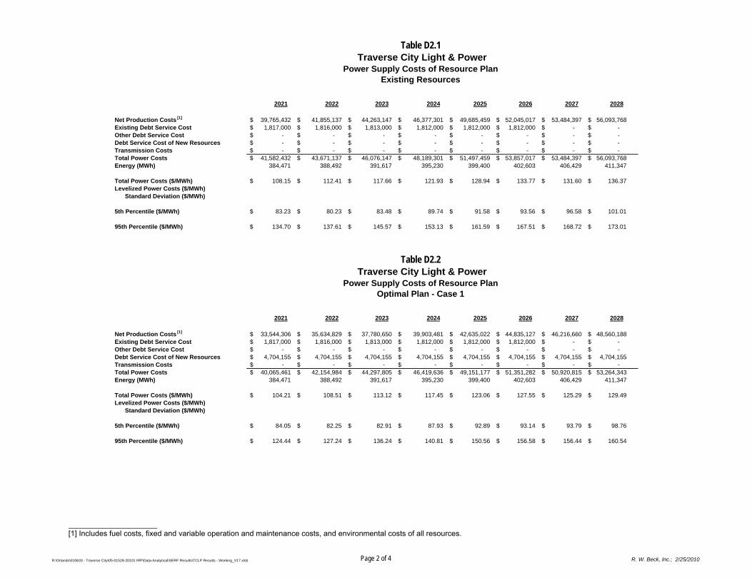
Net Production Costs [1]
Existing Debt Service CostOther Debt Service CostDebt Service Cost of New ResourcesTransmission CostsTotal Power CostsEnergy (MWh)
Total Power Costs ($/MWh)Levelized Power Costs ($/MWh)
Standard Deviation ($/MWh)
5th Percentile ($/MWh)
95th Percentile ($/MWh)
Net Production Costs [1]
Existing Debt Service CostOther Debt Service CostDebt Service Cost of New ResourcesTransmission CostsTotal Power CostsEnergy (MWh)
Total Power Costs ($/MWh)Levelized Power Costs ($/MWh)
Standard Deviation ($/MWh)
5th Percentile ($/MWh)
95th Percentile ($/MWh)
Table D2.1 Traverse City Light & Power
Power Supply Costs of Resource PlanExisting Resources
2021 2022 2023 2024 2025 2026 2027 20281 1 1 1 1 1 1 1
39,765,432$ 41,855,137$ 44,263,147$ 46,377,301$ 49,685,459$ 52,045,017$ 53,484,397$ 56,093,768$ 1,817,000$ 1,816,000$ 1,813,000$ 1,812,000$ 1,812,000$ 1,812,000$ -$ -$
-$ -$ -$ -$ -$ -$ -$ -$ -$ -$ -$ -$ -$ -$ -$ -$ -$ -$ -$ -$ -$ -$ -$ -$
41,582,432$ 43,671,137$ 46,076,147$ 48,189,301$ 51,497,459$ 53,857,017$ 53,484,397$ 56,093,768$ 384,471 388,492 391,617 395,230 399,400 402,603 406,429 411,347
108.15$ 112.41$ 117.66$ 121.93$ 128.94$ 133.77$ 131.60$ 136.37$
83.23$ 80.23$ 83.48$ 89.74$ 91.58$ 93.56$ 96.58$ 101.01$
134.70$ 137.61$ 145.57$ 153.13$ 161.59$ 167.51$ 168.72$ 173.01$
Table D2.2 Traverse City Light & Power
Power Supply Costs of Resource PlanOptimal Plan - Case 1
2021 2022 2023 2024 2025 2026 2027 202814 14 14 14 14 14 14 14
33,544,306$ 35,634,829$ 37,780,650$ 39,903,481$ 42,635,022$ 44,835,127$ 46,216,660$ 48,560,188$ 1,817,000$ 1,816,000$ 1,813,000$ 1,812,000$ 1,812,000$ 1,812,000$ -$ -$
-$ -$ -$ -$ -$ -$ -$ -$ 4,704,155$ 4,704,155$ 4,704,155$ 4,704,155$ 4,704,155$ 4,704,155$ 4,704,155$ 4,704,155$
-$ -$ -$ -$ -$ -$ -$ -$ 40,065,461$ 42,154,984$ 44,297,805$ 46,419,636$ 49,151,177$ 51,351,282$ 50,920,815$ 53,264,343$
384,471 388,492 391,617 395,230 399,400 402,603 406,429 411,347
104.21$ 108.51$ 113.12$ 117.45$ 123.06$ 127.55$ 125.29$ 129.49$
84.05$ 82.25$ 82.91$ 87.93$ 92.89$ 93.14$ 93.79$ 98.76$
124.44$ 127.24$ 136.24$ 140.81$ 150.56$ 156.58$ 156.44$ 160.54$
R:\Orlando\010633 - Traverse City\05-01528-20101 IRP\Data-Analytical\SERF Results\TCLP Results - Working_V17.xlsb Page 2 of 4 R. W. Beck, Inc.; 2/25/2010
_____________________ [1] Includes fuel costs, fixed and variable operation and maintenance costs, and environmental costs of all resources.
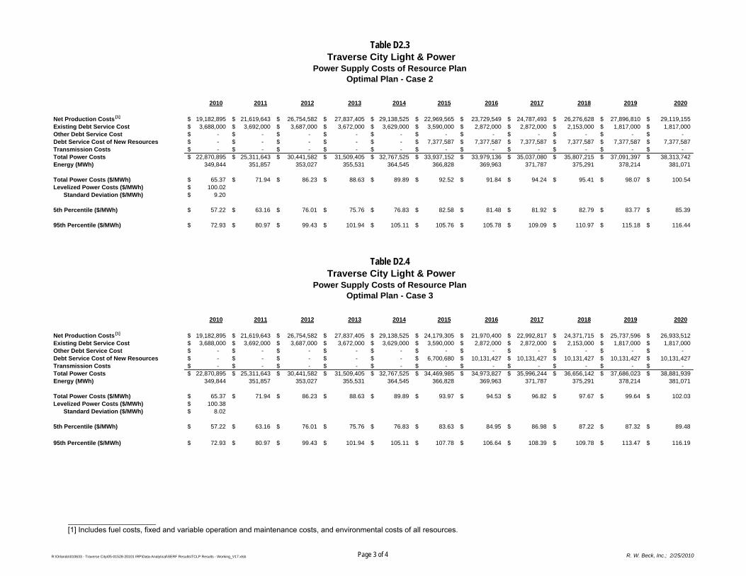
Table D2.3 Traverse City Light & Power
Power Supply Costs of Resource PlanOptimal Plan - Case 2
2010 2011 2012 2013 2014 2015 2016 2017 2018 2019 20201 1 1 1 1 12 12 12 12 12 12
Net Production Costs [1] 19,182,895$ 21,619,643$ 26,754,582$ 27,837,405$ 29,138,525$ 22,969,565$ 23,729,549$ 24,787,493$ 26,276,628$ 27,896,810$ 29,119,155$ Existing Debt Service Cost 3,688,000$ 3,692,000$ 3,687,000$ 3,672,000$ 3,629,000$ 3,590,000$ 2,872,000$ 2,872,000$ 2,153,000$ 1,817,000$ 1,817,000$ Other Debt Service Cost -$ -$ -$ -$ -$ -$ -$ -$ -$ -$ -$ Debt Service Cost of New Resources -$ -$ -$ -$ -$ 7,377,587$ 7,377,587$ 7,377,587$ 7,377,587$ 7,377,587$ 7,377,587$ Transmission Costs -$ -$ -$ -$ -$ -$ -$ -$ -$ -$ -$ Total Power Costs 22,870,895$ 25,311,643$ 30,441,582$ 31,509,405$ 32,767,525$ 33,937,152$ 33,979,136$ 35,037,080$ 35,807,215$ 37,091,397$ 38,313,742$ Energy (MWh) 349,844 351,857 353,027 355,531 364,545 366,828 369,963 371,787 375,291 378,214 381,071
Total Power Costs ($/MWh) 65.37$ 71.94$ 86.23$ 88.63$ 89.89$ 92.52$ 91.84$ 94.24$ 95.41$ 98.07$ 100.54$ Levelized Power Costs ($/MWh) 100.02$
Standard Deviation ($/MWh) 9.20$
5th Percentile ($/MWh) 57.22$ 63.16$ 76.01$ 75.76$ 76.83$ 82.58$ 81.48$ 81.92$ 82.79$ 83.77$ 85.39$
95th Percentile ($/MWh) 72.93$ 80.97$ 99.43$ 101.94$ 105.11$ 105.76$ 105.78$ 109.09$ 110.97$ 115.18$ 116.44$
Table D2.4 Traverse City Light & Power
Power Supply Costs of Resource PlanOptimal Plan - Case 3
2010 2011 2012 2013 2014 2015 2016 2017 2018 2019 20201 1 1 1 1 3 4 4 4 4 4
Net Production Costs [1] 19,182,895$ 21,619,643$ 26,754,582$ 27,837,405$ 29,138,525$ 24,179,305$ 21,970,400$ 22,992,817$ 24,371,715$ 25,737,596$ 26,933,512$ Existing Debt Service Cost 3,688,000$ 3,692,000$ 3,687,000$ 3,672,000$ 3,629,000$ 3,590,000$ 2,872,000$ 2,872,000$ 2,153,000$ 1,817,000$ 1,817,000$ Other Debt Service Cost -$ -$ -$ -$ -$ -$ -$ -$ -$ -$ -$ Debt Service Cost of New Resources -$ -$ -$ -$ -$ 6,700,680$ 10,131,427$ 10,131,427$ 10,131,427$ 10,131,427$ 10,131,427$ Transmission Costs -$ -$ -$ -$ -$ -$ -$ -$ -$ -$ -$ Total Power Costs 22,870,895$ 25,311,643$ 30,441,582$ 31,509,405$ 32,767,525$ 34,469,985$ 34,973,827$ 35,996,244$ 36,656,142$ 37,686,023$ 38,881,939$ Energy (MWh) 349,844 351,857 353,027 355,531 364,545 366,828 369,963 371,787 375,291 378,214 381,071
Total Power Costs ($/MWh) 65.37$ 71.94$ 86.23$ 88.63$ 89.89$ 93.97$ 94.53$ 96.82$ 97.67$ 99.64$ 102.03$ Levelized Power Costs ($/MWh) 100.38$
Standard Deviation ($/MWh) 8.02$
5th Percentile ($/MWh) 57.22$ 63.16$ 76.01$ 75.76$ 76.83$ 83.63$ 84.95$ 86.98$ 87.22$ 87.32$ 89.48$
95th Percentile ($/MWh) 72.93$ 80.97$ 99.43$ 101.94$ 105.11$ 107.78$ 106.64$ 108.39$ 109.78$ 113.47$ 116.19$
R:\Orlando\010633 - Traverse City\05-01528-20101 IRP\Data-Analytical\SERF Results\TCLP Results - Working_V17.xlsb Page 3 of 4 R. W. Beck, Inc.; 2/25/2010
_____________________ [1] Includes fuel costs, fixed and variable operation and maintenance costs, and environmental costs of all resources.

Net Production Costs [1]
Existing Debt Service CostOther Debt Service CostDebt Service Cost of New ResourcesTransmission CostsTotal Power CostsEnergy (MWh)
Total Power Costs ($/MWh)Levelized Power Costs ($/MWh)
Standard Deviation ($/MWh)
5th Percentile ($/MWh)
95th Percentile ($/MWh)
Net Production Costs [1]
Existing Debt Service CostOther Debt Service CostDebt Service Cost of New ResourcesTransmission CostsTotal Power CostsEnergy (MWh)
Total Power Costs ($/MWh)Levelized Power Costs ($/MWh)
Standard Deviation ($/MWh)
5th Percentile ($/MWh)
95th Percentile ($/MWh)
Table D2.3 Traverse City Light & Power
Power Supply Costs of Resource PlanOptimal Plan - Case 2
2021 2022 2023 2024 2025 2026 2027 202812 12 12 12 12 12 12 12
31,105,011$ 33,026,887$ 34,976,465$ 37,011,643$ 39,432,573$ 41,480,548$ 42,848,328$ 45,008,935$ 1,817,000$ 1,816,000$ 1,813,000$ 1,812,000$ 1,812,000$ 1,812,000$ -$ -$
-$ -$ -$ -$ -$ -$ -$ -$ 7,377,587$ 7,377,587$ 7,377,587$ 7,377,587$ 7,377,587$ 7,377,587$ 7,377,587$ 7,377,587$
-$ -$ -$ -$ -$ -$ -$ -$ 40,299,598$ 42,220,474$ 44,167,052$ 46,201,230$ 48,622,160$ 50,670,135$ 50,225,915$ 52,386,522$
384,471 388,492 391,617 395,230 399,400 402,603 406,429 411,347
104.82$ 108.68$ 112.78$ 116.90$ 121.74$ 125.86$ 123.58$ 127.35$
87.42$ 88.38$ 88.49$ 93.25$ 99.00$ 99.19$ 96.96$ 99.32$
121.64$ 123.94$ 131.25$ 135.97$ 143.08$ 150.42$ 148.73$ 154.14$
Table D2.4 Traverse City Light & Power
Power Supply Costs of Resource PlanOptimal Plan - Case 3
2021 2022 2023 2024 2025 2026 2027 20284 4 4 4 4 4 4 4
28,717,483$ 30,495,983$ 32,241,192$ 34,172,720$ 36,294,260$ 38,177,621$ 39,526,285$ 41,525,232$ 1,817,000$ 1,816,000$ 1,813,000$ 1,812,000$ 1,812,000$ 1,812,000$ -$ -$
-$ -$ -$ -$ -$ -$ -$ -$ 10,131,427$ 10,131,427$ 10,131,427$ 10,131,427$ 10,131,427$ 10,131,427$ 10,131,427$ 10,131,427$
-$ -$ -$ -$ -$ -$ -$ -$ 40,665,910$ 42,443,410$ 44,185,619$ 46,116,147$ 48,237,687$ 50,121,048$ 49,657,712$ 51,656,659$
384,471 388,492 391,617 395,230 399,400 402,603 406,429 411,347
105.77$ 109.25$ 112.83$ 116.68$ 120.78$ 124.49$ 122.18$ 125.58$
90.51$ 93.82$ 90.79$ 95.26$ 95.43$ 97.74$ 97.06$ 97.39$
121.25$ 124.53$ 129.49$ 134.86$ 138.08$ 144.13$ 142.57$ 149.66$
R:\Orlando\010633 - Traverse City\05-01528-20101 IRP\Data-Analytical\SERF Results\TCLP Results - Working_V17.xlsb Page 4 of 4 R. W. Beck, Inc.; 2/25/2010
_____________________ [1] Includes fuel costs, fixed and variable operation and maintenance costs, and environmental costs of all resources.

Appendix E LIST OF ACRONYMS

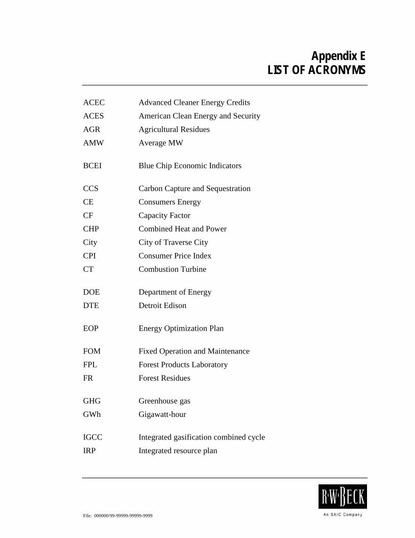
File: 000000/99-99999-99999-9999
Appendix E LIST OF ACRONYMS
ACEC Advanced Cleaner Energy Credits
ACES American Clean Energy and Security
AGR Agricultural Residues
AMW Average MW
BCEI Blue Chip Economic Indicators
CCS Carbon Capture and Sequestration
CE Consumers Energy
CF Capacity Factor
CHP Combined Heat and Power
City City of Traverse City
CPI Consumer Price Index
CT Combustion Turbine
DOE Department of Energy
DTE Detroit Edison
EOP Energy Optimization Plan
FOM Fixed Operation and Maintenance
FPL Forest Products Laboratory
FR Forest Residues
GHG Greenhouse gas
GWh Gigawatt-hour
IGCC Integrated gasification combined cycle
IRP Integrated resource plan

Appendix E
E-2 R. W. Beck Appendix E - Acronyms.doc 2/25/10
kW Kilowatt
kWh Kilowatt-hour
lb Pound
MISO Mid-West Independent System Operator
MMBtu Million Btu
MPPA Michigan Public Power Agency
MUW Mill and Urban Waste
MW Megawatt
MWh Megawatt-hour
NREL National Renewable Energy Laboratories
O&M Operation and Maintenance
ORNL Oakridge National Laboratories
PPA Purchase Power Agreement
PV Photovoltaic
REC Renewable Energy Credits
REP Renewable Energy Plan (specific to Michigan)
RPS Renewable Portfolio Standard
SCP Coal Supercritical Pulverized Coal-fired Steam Plant
SERF Stochastic Econometric Regional Forecasting
SWG Switch Grass
TCLP Traverse City Light and Power
VOM Variable Operation and Maintenance
WDS Wood-waste solids


