1 I. SYLLABUS The course is taught on the basis of lecture notes which can be obtained from my web site ( http://www.niu.edu/∼veenendaal/563.htm ). These notes contain the following topics: I. LITERATURE II. INTRODUCTION A. History up to Newton B. Daniel Bernoulli and the foundations of statistical mechanics C. History from Newton to Carnot D. Thermodynamics E. Atomism III. SYSTEMS OF NONINTERACTING ARTICLES OR SPINS A. Two-level spin system B. History of statistical mechanics: Clausius and Maxwell C. Thermal equilibrium and entropy D. History of statistical mechanics: Boltzmann E. Boltzmann factor G. Free energy H. Ideal gas I. Pressure J. The ideal gas law K. Gibbs’ paradox L. History of statistical mechanics: Gibbs M. Link to classical partition function IV. Quantum mechanics A. Planck’s quantum hypothesis B. Many-particle wavefunctions C. The chemical potential D. Quantum distribution functions V. Systems of interacting particles or spins A. Van der Waals gas B. Critical points C. The Ising model: mean field D. Relations between liquid-gases transition and magnetism E. Ising model: exact solution in one Dimension VI. Applications A. Superfluidity in Helium II
Transcript
1
I. SYLLABUS
The course is taught on the basis of lecture notes which can be obtained from my web site (http://www.niu.edu/∼veenendaal/563.htm ). These notes contain the following topics:
I. LITERATURE
II. INTRODUCTIONA. History up to NewtonB. Daniel Bernoulli and the foundations of statistical mechanicsC. History from Newton to CarnotD. ThermodynamicsE. Atomism
III. SYSTEMS OF NONINTERACTING ARTICLES OR SPINS
A. Two-level spin systemB. History of statistical mechanics: Clausius and MaxwellC. Thermal equilibrium and entropyD. History of statistical mechanics: BoltzmannE. Boltzmann factorG. Free energyH. Ideal gasI. PressureJ. The ideal gas lawK. Gibbs’ paradoxL. History of statistical mechanics: GibbsM. Link to classical partition function
IV. Quantum mechanics
A. Planck’s quantum hypothesisB. Many-particle wavefunctionsC. The chemical potentialD. Quantum distribution functions
V. Systems of interacting particles or spins
A. Van der Waals gasB. Critical pointsC. The Ising model: mean fieldD. Relations between liquid-gases transition and magnetismE. Ising model: exact solution in one Dimension
VI. Applications
A. Superfluidity in Helium II
2
A. Literature
ThermodynamicsR. J. Baxter, Exactly Solved Models in Statistical Mechanics (Academic Press, London, 1982).A. H. Carter, Classical and Statistical Thermodynamics (Prentice Hall, Upper Saddle River, NJ, 2001).R. L. Pathria, Statistical Mechanics (Butterworth-Heinemann, Oxford, 1972). F. Reif, Statistical and ThermalPhysics (McGraw-Hill, Boston, 1965).C. Kittel and H. Kroemer, Thermal Physics (W. H. Freeman and Company, New York, 1980)H. E. Stanley, Introduction to Phase Transitions and Critical Phenomena (Oxford University Press, Oxford, 1971).
Quantum mechanicssee, e.g., my lecture notes for 560/1, http://www.niu.edu/∼veenendaal/p560.pdf.
BackgroundR. D. Purrington, Physics in the nineteenth century (Rutgers University Press, New Bruncswick, 1997).Wikipedia, http://en.wikipedia.org/wiki/Main page.
3
II. INTRODUCTION
A. ***History up to Newton***
We start out this course by recapping in a very condensed form the history of thermodynamics and statisticalmechanics. Throughout the centuries, the basic problems in natural philosophy (as science was called before it wassplit up into physics, chemistry, biology, etc.) can be brought back to several opposites: particles versus waves,discrete/quantized versus continuum. It was only in the late nineteenth and early twentieth century that these issueswere resolved (at least, for the moment). Quantum mechanics shows that the particle and wave nature are bothaspects of the same entity. Statistical mechanics demonstrates that the fact that nature is discrete is not at odds withthe continuous character that we generally experience.
Many ancient philosophies included five elements to explain nature. The elements are earth, water, air (or wind),fire, and aether. The first three describe the three states of matter. In modern terms: solid, liquid, and gas. Thestudy of these different phases is an essential part of thermodynamics. Fire is combustion, and essentially a chemicalreaction, another important element in thermodynamics, although not really a part of this course. The fifth element,aether, is more complicated and we return to that in a while. In Greek philosophy these concepts were listed byEmpedocles (ca. 450 BC), although the same concepts already appeared much earlier in Asia, where it forms thebasis of Buddhism and Hinduism. The ideas of the five elements have had a profound influence on western civilizationand philosophy, medicine, and science. In Greek philosophy, the ideas were worked out by Aristotle (384 BC-322 BC),one of the most important persons in western thought. Aristotle was a student of Plato and a teacher of Alexanderthe Great. Unfortunately, the effect on the progress of science was not always positive. We cannot blame Aristotle forall of this. First, he was a philosopher and not a natural philosopher, more interested in the “why” than the “how”.Renaissance scientist, such as Galileo, suffered particularly from the fact that Aristotle’s ideas were taken over by thecatholic church, and turned into a dogma as opposed to a theory. Since we are indoctrinated by Newtonian thinking,it is difficult to consider ancient Greek thought without dismissing it directly. First, we have have to understand howrevolutionary the ideas of Galileo, Newton, and others were. Nowadays, we make a big deal of Einstein imagining howit would be like to move at the speed of light, but the approach of is not unlike that in classical physics. The crucialbreakthrough is to imagine the laws of nature in an ideal world. We find it completely natural that the Newton’s lawsare first discussed in an ideal world and that subsequently all the aspects of the real world (friction, drag, etc.) areintroduced. For most Greek philosophers, this was unacceptable. Why first describe something in an unreal worldand then try to describe the real world. For Aristotle, resistance was essential in his way of thinking. Newton’s
AristotleParmenides Democritus
FIG. 1: The greeks Parmenides and Aristotle argues against the existence a void (or vacuum). The opposed the ideas ofLeucippes and Democritus that everything was made out of indivisible particles (atoms) inside a void.
4
second law states, in one dimension, F = ma = m d2xdt2 . In the absence of forces, this gives d2x
dt2 = 0 or dvdt = 0 or
v = constant. This is Newton’s first law. Newton’s first law is contained in his second. Obviously, Newton was awareof this. However, he felt it necessary to state it separately (the question remains why, after more than four centuries,we still have to teach it that way). The reason is that it is unnatural and contradicting centuries of thought. It isunnatural since it is perfectly obvious to everyone that the velocity is not constant in the absence of a force. Aftera while, everything comes back to its natural state of rest. The Greeks had a more intuitive approach to laws thatwork in a real world. Objects have a nature. Why do rocks fall down? Because rocks are earth-like and it is in theirnature to be with the rest of the earth. That’s where they would like to move to. Feathers and leaves on the otherhand are in between air and earth and fall much more slowly. Makes perfect sense. It also explains why rocks fallmore slowly in water, because rocks are close to water than air. However, in the end everything comes back to rest.In fact, you require a force to move objects. Again, completely natural. To get somewhere you need to move yourmuscles. This whole concept of constant velocity in the absence of a force is completely ludicrous. In fact, some havecredited Aristotle with the effective equation that the moving force can be written (in a very modern notation) asF = Rv, where R is the resistance and v is the velocity that you want (this is probably not what Aristotle meant,but often the interpretations of Aristotle’s works are just as important as what was actually written). And probablya significant percentage of the world population would believe this law.
You might have heard this when discussing classical mechanics, but what does this have to do with thermodynamics.Well, things go horribly wrong when we go to Newton’s ideal world or, as Aristotle would put it, the unreal world.Let imagine the motion in a void or vacuum. (And to give the Greeks credit, they did think about this. They noticedthat their conception lead to contradictions and they were not afraid to confront these issues. They were open todiscussion, unlike the centuries preceding Galileo). There are a number of problems. First of all, if it is in the natureof things to fall down, then what does an object do in a void. It would not like to go anywhere, because it would bein his nature to go to earth, which is absent in a void. So there is no motion in a void. Now what happens, when weapply a force. Well, since v = F/R, the velocity would be infinite and the displacement would be instantaneous. Sincethis is absurd, Aristotle against a vacuum and proclaimed his dictum of horror vacui or “nature abhors a vacuum”which was firmly states in his influential book Physics. Arguments against the void where already given more thana century before Aristotle, by Parmenides in ca. 485 BC. Parmenides argues against motion in a void, because avoid is nothing and does not exist. If you move in there then something would come out of nothing, but ex nihilonihil fit or nothing comes from nothing. Arguments against this were brought up by Leucippus, which written downand elaborated by Democritus (ca. 460 BC-370 BC). They proposed the, in our modern eyes, very appealing ideasthat void was everywhere but filled with indivisible particles (atomos). The particles could have different shapes,size, and weights. Everything was made up of these tiny particles, or, in Democritus’ words: “By convention sweet,by convention bitter, by convention hot, by convention cold, by convention color, but in reality atoms and void.”Although revolutionary, the ideas were rejected by most Greeks. A nice idea to make up these particles, but nobodyhas ever seen them. Certainly ideas that still lived in the nineteenth century when Boltzmann and others weredeveloping statistical mechanics. In addition, atomism, as it is commonly called, still requires moving in a void, whichis impossible according to Aristotle.
This brings us to the fifth element. Surprisingly, many ancient cultures include this fifth element. Apparently, thefour “earthy” ones, earth, water, air, and fire, were insufficient for a complete understanding of nature. Clearly, inAristotle’s world view the sky posed a problem. The moon and sun are obviously heavy entities and it would be intheir nature to fall to earth. However, this does not happen, therefore they must be moving around in some othermedium. This medium is called the aether. Obviously, they could not be moving around in a void, since that doesnot exist. The sky or the heavens is also where the God/Gods live and the aether is often also used to describeeverything else that exists outside the material world, such as thoughts, ideas, love, etc. It is therefore quintessentialto life itself (note that quinta essentia means fifth element). The word aether comes from “pure, fresh air” or “clearsky” in Homeric Greek and was the pure essence that the Gods breathed as opposed to the aer that regular mortalsbreathe. Aether had no qualities such as hot, cold, wet, or dry, as opposed to the other elements. In hinduism aetheris called akasha. If was from the akasha that all the other four elements were made. Certainly, a very appealingconcept in modern physics which claims that at the time of the Big Bang, the universe was created out of nothing. Tounderstand the impact of these philosophies, if only suffices to realize that it was not until 1887, that modern sciencewas finally able to start leaving the aether behind with the Michelson-Morley experiment.
It is against this background that the scientific work started in the renaissance. Centuries of thought had gone intothe current understanding of the world. Many thoughts were wrong, but not entirely unreasonable. Rethinking ofthermodynamics started when Galileo Galilei (1564-1642) was asked a question about siphon in ca. 1643. Siphon isjust the Latin and Greek word for tube. We can use a continuous tube to drain liquid from a reservoir through a higherpoint to another reservoir. The final end of the tube has to be lower than the liquid surface in the reservoir, see Fig. 1.The principle of syphoning was already known to the Egyptians and the Greeks and described by Hero of Alexandria(10-70 AD) in his treatise Pneumatica. The common understanding is that, since the liquid flows out at the end of the
5
tube, a vacuum is created in the tube. However, since nature abhors a vacuum, liquid is sucked into the tube. In themiddle ages, the technique was used to drain mines (and in this day and age, it is still used to steal the gas from yourtank). In 1630, Galileo was asked by Giovan Battista Baliani of Genoa why a syphon he had contructed to carry waterover a 21 meter high hill failed. Galileo had ascertained that there were apparently limitations in the vacuum forceand the maximum intermediate height was about 18 braccia (around 11 meters). Galileo’s interpretation, although,as we know now, being incorrect, stimulated further research by Evangelista Torricelli (1608-1647) and others. Theexperiment was simple. Instead of using water, Torricelli used a much heavier liquid: mercury. He filled a tube withmercury, closed the top with his finger and put it upside down in a basin and removed his finger. The mercury droppedand stopped at a height of 76 cm. Torricelli arrived at two important and revolutionary conclusions. First, he hadcreated a vacuum inside the tube. Second, he was convinced it was not the sucking force of the vacuum holding themercury in the tube, but the weight of the air pushing the mercury in the tube. Additional experiments by, amongother, Blaise Pascal (1623-62), Gilles Personne Roberval (1610-1675), and Robert Boyle (1627-1691) demonstratedthe validity of his arguments. Performing the experiment in vacuum (the void within a void) showed that the absenceof air resulted in the complete emptying of the tube. Coincidentally, Torricelli had also invented the barometer.This was followed by Blaise Pascal demonstration that the atmospheric pressure depends on altitude in the famousexperiment in 1648 on the Puy-de-Dome.
After Torricelli’s demonstration of the vacuum, Otto van Guericke was the first to create a vacuum using a simplevacuum pump consisting of a piston and a cylinder with one-way flap valves in 1650. He used this to suck the airout of two copper hemispheres with mating rims which were then tightly held together by the air pressure of thesurrounding atmosphere. This was famously demonstrated in front of emperor Ferdinand III and the Reichstag inRegensburg in 1654 where two teams of 15 horses were unable to separate the two hemispheres. This experiment wasrepeated in Magdeburg in 1657 and the experiment is also know as that of the Magdeburg hemispheres. The vacuumpump was further perfected by Robert Boyle and and his assistant Robert Hooke (1635-1703). Among other things,they demonstrated that there is no sound in vacuum, demonstrating that sound needs a medium to propagate. Inaddition, vacuum helped classical mechanics. Although Galileo had already postulated that object fall in the sameway irrespective of their weight, shape, and size, this was only convincingly demonstrated by actually performing theexperiments in vacuum.
Robert Boyle was an influential natural philosopher. He could be described as a gentleman scientist, being born inIreland as the seventh son and fourteenth child of Richard Boyle, the “Great Earl of Cork”. He was highly educatedand learned Latin, Greek, and French as a child, was sent to Eton College. After three years in college, he embarked
Galileo GalileiEvangelista Torricelli
Torricelli's experiment
Siphon
Roberval's experiment of a void within a void
FIG. 2: Stimulated by Galileo Galilei’s ideas that the reason that the intermediate height for a syphon was limited by themaximum strength of the vacuum force, Evangelista Torricelli performed his own experiments demonstrating the existence of avacuum and the weight of air. Roberval’s and others’ reproduction of Torricelli’s experiment in a vacuum (void within a void)demonstrated that it was indeed the weight of air keeping the mercury up since in vacuum the tube emptied.
6
on a grand tour with a French tutor (the term tourism is arrived from this. A typical rite of passage for wealthyBritish upper class men). He spent two years in Geneva and was in Florence in the winter of 1641. (Note, that Robertwas only 14 at the time). It is worthwhile to remember that Galileo Galilei died in early 1642 within three miles of thegreat renaissance city. In 1645, his sick father left him Stalbridge manor in Dorset in Southern England. Boyle waspart of the “invisible college”, (first mentioned by Hooke in 1646) a group of scientists interested in pursuing ideason this new natural philosophy. The group included John Wallis (1616-1703), who was an important figure in thehistory of calculus, crucial for the development of classical mechanics. He also introduced the symbol ∞ for infinity;Robert Hooke, Boyle’s assistant, who played a role in many areas. Hooke is known for Hooke’s law (F = −Kx), butalso coined the term cell because his observation of plant cells reminded him of monks’ cells; Sir. Christopher Wren(1632-1723). Wren is known to the general public as an architect. He was appointer the King’s surveyor of Works in1669, after the Great Fire of 1666 had destroyed two-thirds of London. Apart from designing St. Paul’s cathedral, hewas responsible for the rebuilding of 51 churches. He also contributed to astronomy and geometry. They correspondedthrough letters, before the existence of scientific journals. The informal and somewhat secretive societies formed theseeds for the foundation of the Royal Society in 1660. Robert Hooke served a Curator of Experiments, Wren wasa co-founder and served as president. It had a great influence in the reporting and dissemination of science in thePhilosophical Transactions of the Royal Society of London (which is the oldest English scientific journal and stillexists. The oldest was French Journal des Savants). Robert Boyle was also influential through his extensive writings.His book The Sceptical Chymist (1661) is seen as a milestone in the field of chemistry. It denied the limitations tothe classic four elements. It pushed chemistry to the same level as medicine and (yes!) alchemy. Boyle insisted thatall theories must be verified experimentally.
Of more importance to us is that Boyle also wrote down one of the first quantitative laws in thermodynamics,known as Boyle’s law. In modern form this is written as
PV = constant, (1)
where P is the pressure and V is the volume. Although, this is certainly not a form that Boyle would have recognized.We are so used to our modern mathematical and physical tools that certain results look entirely trivial. Boyle wrote:till further trial hath more clearly informed me, I shall not venture to determine, whether or no the intimated theorywill hold universally and precisely, either in condensation of air, or rarefaction: all that I shall now urge being, that. . . the trial already made sufficiently proves the main thing, for which I here allege it; since by it, it is evident,that as common air, when reduced to half its wonted extent, obtained near about twice as forcible a spring as it hadbefore, so this thus comprest air being further thrust into half this narrow room, obtained thereby a spring about asstrong again as that it last had, and consequently four times as strong as that of the common air. It is clear that ourmodern mathematical tools greatly simplify our work and make it difficult for us to understand why it took so long forsomebody to come up with something simple as PV =constant. Getting a nail in the wall looks easy when somebodyhad already invented the hammer, but try to imagine doing it without a hammer. Boyle did not invent this law, hewrote it down in 1662. It was actually discovered by two friends and amateur scientists Richard Towneley and HenryPower. The law was also discovered independently by Edme Mariotte (1620-1684) in 1676 (note that this is 14 yearslater!). In some countries, it is therefore known as the Boyle-Mariotte law. (Interestingly, as another example of thewide range of topics scientists studied in those days as opposed to the narrow-minded scientists of today, Mariotte wasthe first to describe the eye’s blind spot. An interesting flaw in nature’s/God’s design of the eye. The optical nervesare attached to the receptors at the inside of the eye. This forces the optical nerves to exit the eye at some pointwhere the are no optical receptor. Strangely enough, it is only cephalopods (squids and such) where nature/God gotit right and let the optic nerve approach the receptors from behind, so that there is no need to break the retina).Combined with Charles’ law (1787): V/T = constant, where T is the temperature; Gay-Lussac’s law (1802): P ∼ T ;Avogadro’s principle (1811) V/n = constant, where ν is the number of moles in the gas, this finally constituted theideal gas law PV = νRT , where R is the gas constant, which was first stated by Clapeyron in 1834. That only tookabout 170 years.
However, we are drifting off and racing ahead. No overview can be complete without Isaac Newton (1643-1727).His phenomenal work Philosophiae Naturalis Principia Mathematica (Mathematical Principles of Natural Philosophy,shortly known as the Principia) laid the basis for all classical mechanics to come. It also is a giant leap forwardin the development of calculus which was firmly established by Newton and Gottfried Wilhelm Leibniz (1646-1716).Newton’s achievements in calculus and classical mechanics are one of the most influential, if not the most influential,contributions in science. His contributions to classical mechanics should be well known to every student of physics.Newton also made significant contributions to optics. He advocated that light consisted of corpuscles, although he didnot really stress this point. Although again this looks appealing from our modern photon concept of light, Newton’sideas are far removed from the quantum-mechanical framework. However, these ideas came under fire by scientistswho believed in the wavelike nature of light such as Robert Hooke and the Dutch scientist Christiaan Huygens (1629-1965). This led Newton to withdraw from public life to about a decade. However, even though the wave representation
7
was a better approach to light at that time, Newton’s influence was such that the particle theory of light dominatedfor the next century.
B. Daniel Bernoulli and the foundations of statistical mechanics
The Bernoullis were a Swiss family containing eight prominent mathematicians, including Jacob Bernoulli (1654-1705), who discovered the Bernoulli numbers (which are related to the Riemann zeta function and therefore to one ofthe famous unsolved problems in mathematics: the Riemann hypothesis); his brother Johann Bernoulli (1667-1748)solved the problem of the catenary or the hanging flexible cable. He was professor at the University of Groningen inthe Netherlands, when his son Daniel Bernoulli (1700-1782) was born. His father pushed him to become a businessman, but in the end, he choose mathematics. The relationship with his father significantly deteriorated when theyboth entered a scientific contest from the University of Paris. His father could not bare the shame of having toshare the first prize with his son. As a return favor, he even tried to steal Daniel’s book Hydrodynamics and recallit Hydraulica. Daniel Bernoulli also work on a new theory on the measurement of risks which was the base of theeconomic theory of risk aversion and premium and did significant work on statistics by analyzing the morbidity ratesfrom small pox in 1766. Daniel Bernoulli also worked on flow and is the one behind the Bernoulli equation, whichrelates pressure, velocity and height in the steady motion of a fluid.
Daniel Bernoulli, in 1738, was the first to understand air pressure from a molecular point of view. He considered avertical cylinder closed at the bottom and with a piston and a weight at the top. The piston’s weight was supportedby the air pressure. Or in Bernoulli’s words: “let the cavity contain very minute corpuscles, which are driven hitherand thither with a very rapid motion; so that these corpuscles, when they strike against the piston and sustain it bytheir repeated impacts, form an elastic fluid which will expand of itself if the weight is removed or diminished. . . ”.Brilliant! Unfortunately, very few accepted this view. Most people were convinced that gas molecules stayed more orless in the same place repelling each other held together by the aether. Let us derive a modern version of the kinetictheory. Consider a box in which particles are moving with a velocity v (this can be generalized to average velocities,but for simplicity let us assume that the velocity is constant). The momentum p of a particle moving towards the wallis then p = mv. If it bounces of the wall elastically, the momentum after the colission is p = −mvx. Its momentumchange is then −2mv, so the momentum transferred to the wall is 2mvx. If the density of particles is n = N/V thenthe total number of particles hitting the wall in a time ∆t is 1
2nAvx∆t, since half of the particles within a distance
Daniel Bernoulli
FIG. 3: Daniel Bernoulli and his illustration of the kinetic theory of gases from Hydrodynamica (1738).
8
v∆t will hit the wall. The other half is moving in the opposite direction. The total momentum transferred to thewall is then ∆p = 2mvx × 1
2nAvx∆t = nAmv2x∆t. The force exerted is then
F =∆p
∆t= nAmv2
x. (2)
The quantity vx is one third of v2, since v2 = v2x + v2
y + v2z . The pressure P is the force per surface area which is
P =F
A= nmv2 =
Nmv2
3V⇒ PV =
1
3Nmv2 =
2
3NEkin, (3)
where Ekin is the average kinetic energy per particle. This is Boyle’s law if the term on the right hand side is constant.As said before this theory was neglected. This is not yet the ideal gas law. The relation between the kinetic energyand the temperature was first realized by John James Waterston (1811-1883) in the nineteenth century in an equallyneglected book. Certainly, the title of the book, published at his own costs, Thoughts on the Mental Functions (1843)was not helpful. In modern notation, average kinetic energy can be written as Ekin = 3
2kBT , which we shall prove inthis course. This yields the ideal gas law
PV = NkBT. (4)
C. ***History from Newton to Carnot***
The eighteenth century saw the great developments of the first engine. The first engine was patented by ThomasSavery (1650-1715) in 1698. It was an early steam engine designed to pump water out of mines. Since the lifting effectof atmospheric pressure was limited to 30 feet, additional pressure coming from steam was used to increase the liftup to 50 feet. The machine used no pistons and was never applied successfully. Following Savery’s design and furtherideas by the Frenchman Denis Papin, Thomas Newcomen (1663-1729) made a more practical devise using a piston.Steam was injected into a cylinder from a boiler. The steam was then condensed and air pressure pushed down thepiston, which was connected to the pump. Note that the real force is the atmospheric pressure since the pressure ofthe steam is limited. Further developments were made by James Watt (1736-1819) in the period 1763 to 1773. Watt’smachine was the first to actually use the steam pressure above atmospheric. Watt noticed that Newcomen’s engine
Newcomen's steam engine Watt's steam engine
FIG. 4: The steam engines by Thomas Newcomen and James Watt to pump water out of mines. Note that the designs arevery similar. The major difference is the introduction of the separate condenser. Other improvements in manufacturing alsoallowed Watt’s machine to use steam pressure larger than atmospheric pressure.
9
was very inefficient. The major idea is the introduction of a separate condenser. When the piston reaches the top, theinlet valve is closed and the passage to the condenser is opened. This has the great advantage that the cylinder canremain hot and the condenser can remain cool, as opposed to having both processes take place in the same cylinder.This allows a great increase in speed. Another improvement was to have the downward motion of the piston doneby low pressure steam as opposed to atmospheric pressure. Also the hot water in the condenser was removed by avacuum pump and recycled into the boiler.
The theoretical understanding also made significant progress. However, the ideas of atoms and the corpusculenature of light actually receded. One of the things we have to realize is that the concept of conservation of energy didnot exist in the eighteenth century and the early nineteenth century. Early pioneers such as Leibniz already noticedin the later seventeenth century the conservation of the quantity (in modern notation)
∑
imiv2i . This he called the
vis viva of the “living force”. Other claimed that the quantity∑
imivi was the vis viva. Of course, we know that inelastic collisions both are conserved. However, for inelastic collisions, this is no longer correct, and some of the energygoes into heat. It was early on suggested that heat is related to the motion of atoms by natural philosophers, such asNewton, Boyle, and John Locke. Or in Boyle’s words: “heat seems principally to consist in that mechanical propertyof matter we call motion”. However, later on this was replaced by the caloric theory, which assumed that heat wasfluid that flows from hotter to colder bodies or a weightless gas that moves in and out of the pores of solids andliquids. This confusion arose partly in the study of combustion. The seventeenth century had seen the development ofthe phlogiston theory by Johann Joachim Becher. The idea was that phlogiston was contained in combustible bodiesand released during combustion. Nowadays we know that combustion is related to oxidation. However, the mistake isnatural since many organic compounds get lighter during combustion since, e.g. water, CO, and CO2, escape duringthe combustion. Since chemical reactions often release heat, the identification of heat as a substance appears morenatural. This was corrected by the great French scientist/chemist Antoine Lavoisier (1742-1794) and laid the correctrelation between combustion and oxidation. Materials therefore become heavier under combustion. Since at the sametime their temperature rises. This appears in support of the caloric theory introduced in 1750 by the Scottish physicistJoseph Black (1728-1799). Black discovered latent heat. Latent heat is the heat that, for example, ice absorbs whenit melts without change in temperature. Black noted that without latent heat a minute change in temperature wouldlead to the immediate melting of all the ice, in contrast with observation. Black concluded that heat was a liquid thatcombines with the material. The term latent comes from the Latin latere, to lie hidden. Lavoisier also introduced theconcept of conservation of mass. Another statement that we all take for granted nowadays, but that was not at allobvious (we are leaving out radioactivity for the moment).
Another reason for the retreat of the atomic idea was the great success of continuous theories. Apart from the theoryof Daniel Bernoulli, little else was achieved based on atomic principles. On the other had, significant progress was madein many areas using continuous models, especially through the development of differential equations. Joseph-Louis,comte de Lagrange (1736-1818) formulated, what is now known, as Lagrangian mechanics. Pierre-Simon Laplace(1749-1827) applied them in his theory of potentials. Joseph Fourier (1768-1830) applied an infinite series to studyheat flow building on Newton’s law of cooling. He was the first to treat heat conduction as a boundary value problemin the theory of partial differential equations. His idea that functions can be expanded in an infinite series had a greatimpact.
At the same time the foundations were laid for the theory of electricity and magnetism. Initial work was mainlyelectrostatics, such as the work by Charles-Augustin de Coulomb (1736-1806) in the 1780’s on the strenght of theCoulomb interaction. Following Galvani’s discovery of bioelectricity in 1783, Alessandro Volta invented the batteryin 1800. The use of electrochemical reactions as opposed to the use of discharges from capacitors such as the Leydenjar (not to mention the outright dangerous methods of Benjamin Franklin) greatly facilitated research in this field.Andre-Marie Ampere (1775-1836) discovered the relationship between electricity and magnetism. This was followedby the very extensive work by Michael Faraday (1791-1867), discovering electromagnetic induction in 1831 and layingthe basis for the electromotor. This finally culminated in the work of James Clerk Maxwell (1831-1879) combiningelectricity and magnetism in four equations (okay, he orginally had twenty), known today as Maxwell’s equations.Electromagnetism was a continuous theory and certainly removed the ideas of corpuscular light proposed by Newton.Note that in the early nineteenth century electricity was also interpreted in terms of an electric fluid.
D. Thermodynamics
The early nineteenth also saw the foundations of thermodynamics. Obviously, few can claim to be the founder ofanything, but the formulation of the Carnot cycle is generally considered an important milestone in the theory ofthermodynamics. Nicolas Leonard Sadi Carnot (1796-1832) was a French physicist and military engineer. Note thedominance of French science in this period. One of the reasons for this is the French revolution and the institution-alization of science and the, at the same time, the foundation of the Ecole normale and Ecole polytechnique in the
10
1790’s. This provided a great boost for science in France. Science is becoming a affair of the state, as is commonnowadays. Carnot went to the Ecole polytechnique. Many scientists were trying to understand the new steam enginesthat were turning the world upside down in an industrial revolution (note that, unlike in electromagnetism, sciencewas more a follower of the technological developments). Carnot’s work “Reflections on the motive power of heat andengines suitable for developing this power” (1824) is by many viewed as laying the foundation of modern thermody-namics. Carnot adhered to the caloric, although later in life he changed his view and became convinced that heat isrelated to the motion of atoms. In his work Carnot laid the basis for the second law of thermodynamics which statesthat the entropy of an isolated system not in equilibrium will tend to increase over time, appraoching a maximumvalue at equilibrium. A very basic consequence of that is that heat flows from a hotter to a cooler body. One doesnot observe that when two bodies are brought into contact that the cooler body becomes cooler and the hotter bodyhotter. Carnot was the first to consider full cycles of engines. He discovered that the work done by the engine is afunction only of the the differential between the hold and cold reservoirs between which it operates. Later on, it wasderived that the efficiency of an idealized engine is given by (T1 − T2)/T1, where T1 is the absolute temperature ofthe hotter reservoir.
Carnot’s work was put on a firmer mathematical framework by Benoıt Paul Emile Clapeyron (1799-1864). Clapeyron
studied at the Ecole polytechnique and Ecole des Mines and left for Saint Petersburg to teach at the Ecole des TravauxPublic (note that the educated people in Russia spoke French and not Russian). He returned to Paris and supervisedthe construction of the first railway line connecting Paristo Versailles and Saint-Germain. Clapeyron devised agraphical representation of the Carnot cycle, developed the ideas of reversible processes, and more firmly establishedthe Carnot principle, which is now known as the second law of thermodynamics.
The years following the death of its strong advocate Laplace in 1827, the caloric theory went into decline. Crucialearly experiments (predating Laplace’s death) were done by Benjamin Thompson (Count Rumford, 1753-1814) andHumphrey Davy (1778-1829). Thompson gave a famous paper to the Royal Society on the heat in cannon boringsin 1798. Obviously, people had already realized that friction created heat. Thompson tried to measure the weight ofthe caloric fluid. The heat created in cannons is huge, however, the resulting loss in weight was zero. Davy presentedrelated work on the the melting of ice due to friction in 1799. Although serious setbacks for the caloric theory, manyscientists including William Thompson (Lord Kelvin) were not converted until the mid nineteenth century. Importantsteps were made by James Joule (1818-1889), an English physicist (and brewer) who studied the relationships betweenmechanical work and heat and laid the foundations for the law of conservation of energy. It is important to note thatthis important relationship (practically the basis of physics) was not established until the nineteenth century. One ofthe experiments performed by Joule is now known as Joule heating. In 1841, at the age of 23, Joule determined theheat loss I2R by a current I flowing through a resistance R by placing the coil in water and carefully measuring therise in temperature. He greatly generalized his work into a more general understanding of the interconvertability ofdifferent types of energy into each.
In 1850, the work of Carnot was put on a firmer basis by Rudolph Clausius. Clausius was born in the provinceof Pomerania in Prussia. In his Ph.D. work at the University of Halle he explained that the sky is blue due to therefraction of light. He then became professor of physics at the Royal Artillery and Engineering School in Berlin. In1855 he moved to the ETH in Zurich. Later in life he also taught in Wurzburg and Bonn. His most famous work is“On the motive power of heat, and on the laws which can be deduced from it for the theory of heat” in the PoggendorfAnnalen in 1850. After several paper published by Clausius and William Thomson, this work presented the secondlaw of thermodynamics for the first time in its complete form. Clausius defined entropy as S = Q/T , where T is theabsolute temperature. He also introduced the name after the Greek word τρoπη meaning transformation. He addedthe en- to make it sound similar to energy. Clausius also considered reversible and irreversible processes. Clausiusalso obtained an explicit form of the first law of thermodynamics in the familiar form dQ = dE + pdV .
Around the same time, William Thomson (1824-1907) devised the absolute energy scale, about which scientists hadalready speculated as early as Guillaume Amontons in 1702.
E. Atomism
Although we have seen that the ideas of atoms already existed in the support for the ideas of atoms was acually at alow point in the early and mid nineteenth century. Thermodynamics and many other theories worked very well in theabsence of the assumption that everything is made up of small indivisible particles. In fact, continuum theories hadmade significant more progress than atomistic theories. The atomistic nature of matter was a largely unsupportedhypothesis. In the early 1800s, apart from Bernoulli’s work, atomism was more a philosophical speculation.
Atomism’s resurgence started in chemistry. Chemistry had its foundations in the decades around 1800 with Priestley,Lavoisier, Dalton and Avogadro. It was John Dalton (1766-1844) who is generally credited with establishing chemistryon atomic principles. He was influenced strongly by Newton who assumed a static atomic model. A model of a gas
11
based on random motions was not proposed until 1738. Atoms were assumed to be massy and hard. The strongsupport for an atomistic model in chemistry is obvious. For example, two volumes of hydrogen combine with one ofoxygen to produce water. Although some aspects were correct, other were less: Dalton assumed that matter was heldtogether by attractive (gravitational) forces. The atoms were kept apart by the repulsive force of the caloric (the heatliquid). Other chemists were also crucial in propagating the atomic theory. The French chemists Pierre Louis Dulong(1785-1838) and Alexis Therese Petit (1791-1820), both at the ecole polytechnique, discovered that the specific heatof a body was directly related to its atomic weight, which is now known as the Dulong-Petit law.
In physics, the atomic principles were pushed by Davy and Faraday. They adhered to the point atomism ideas ofwritten down by Roger Boscovich in his Theory of Natural Philosophy in 1763. Faraday was strongly influenced byhis work in electrochemistry (together with John Daniell). He established the second law of electrochemistry in 1833which asserts that “the amounts of bodies which are equivalent to each other in their ordinary chemical action haveequal quantities of electricity naturally associated with them.” Or, the quantities of different elements deposited by agiven amount of electricity are in the ratio of their chemical equivalent weights. Note that this implies a quantumof electricity, in effect the electron. Faraday had a problem with his picture of point-like atoms. If a solid is madeof point-like atoms that do not touch each other, then what is causing the conduction. Certainly, not the space inbetween since how could there be insulators if the space is responsible? Obviously, Faraday was also concerned withthe propagation of forces. Early on, he had believed that forces were transmitted by contiguous particles. Later on,he changed his ideas into the presence of force fields, while still clinging on to the presence of point-charge atoms insolids.
Although all the arguments in favor of the existence of atoms sound very convincing to our modern ears, manyphysicists remained unconvinced until the end of the nineteenth century. William Thomson wrote: “The idea ofan atom has been so constantly associated with incredible assumptions of infinite strength, absolute rigidity, mysticalaction at a distance, and indivisibility, that chemists and many other reseasonable naturalists of modern times, losingall patience with it, have dismissed it to the realms of metaphysics, and made it smaller than anything we can conceive.”Despite this statement, Lord Kelvin went on to calculate the size of atoms and ended up with a surprisingly accuratevalues of 10−10 m, although he had a preference for vortex atoms. One might wonder how one can do electrostaticswithout the presence of point charges. However, here one can view the point charge as a mathematical devise tocalculate continuous properties. There is no direct need to associate the point charge with an atom. It is against thisbackground that the uphill battle for a discrete theory of mechanics starts employing the use of statistics.
III. SYSTEMS OF NONINTERACTING PARTICLES OR SPINS
A. Two-level spin system
Before discussing the historical developments of statistical mechanics, let us first develop some feeling for statisticswhen dealing with large numbers of particles. One of the simplest system that can be studied is a two-level system.This problem is equivalent to flipping coins.
See A. J. Kox, Eur. J. Phys. 18, 139 (1997); Kittel-Kroemer chapter 1
A more physically relevant two-level system is a set of spins in a magnetic field B. The splitting of energy levelsunder a magnetic field was first observed in the spectral lines of Sodium by the Dutch physicist Pieter Zeeman (1865-1943) in 1896 at the University of Leiden. His colleague at the university was the great Dutch physicist HendrikAntoon Lorentz (1853-1928). Lorentz is known for the force named after him, which describes the force F acting on aparticle with charge q moving at a velocity v in a magnetic field B, F = qv ×B. Lorentz and Zeeman assumed thatthe particles were moving in an harmonic potential (comparable to a spring). This leads to the classical equations ofmotion
md2x
dt2= −Kx+ eB
dy
dt(5)
md2y
dt2= −Ky − eB
dx
dt(6)
md2z
dt2= −Kz (7)
The solution of the latter is a simple harmonic motion z = A cosω0t. Inserting gives a angular frequency ω0 =√
K/m.
12
Two solutions are found for the xy plane
x = A cosω±t and y = ∓A sinω±t (8)
Inserting gives
−ω2± cosω±t = −ω2
0 cosω±t∓eB
mcosω±t (9)
±ω2± sinω±t = ±ω2
0 sinω±t+eB
msinω±t (10)
giving
ω2± ∓ eB
mω± = ω2
0 . (11)
Taking ω± = ω0 ± ∆ω gives
(ω0 ± ∆ω)2 ∓ eB
m(ω0 ± ∆ω) = ω2
0 . (12)
For small ∆ω, (ω0 ± ∆ω)2 ∼= ω20 ± 2ω0∆ω. This gives
2ω0∆ω =eB
mω0 ⇒ ∆ω =
eB
2m(13)
When Zeeman and Lorentz evaluated the e/m ratio, they found a value much larger than expected. This is of coursedue to the fact that the mass of the electron is 9.1×10⁻³¹ kg whereas the mass of a ion is related to the mass of protonsand neutrons 1.67× 10⁻²⁷ kg. Essentially they discovered the electron. Although they were puzzled about the value,they did not put a lot of emphasis on it, focusing on the interpretation of the spectral line shapes. However, this was1896, a year before Joseph John Thomson published his famous experiments on the cathode ray tube. FortunatelyZeeman and Lorentz went on to win the Nobel prize for the Zeeman effect in 1902, whereas J. J. Thomson won it in1906 for the discovery of the electron. For the energy, we can write
E = ~ω − µBB, ~ω, ~ω + µBB, (14)
where µ = e~
2m is the Bohr magneton. Note that the identity E = ~ω was not known to Zeeman and Lorentz sincethis was proposed by Planck in 1900. In a quantum-mechanical notation we have
E = −µ ·B with µ = µBL, (15)
where µ is magnetic moment and the L is the angular momentum. Along the z axis, Lz takes on the valuesLz = −1, 0, 1 for a p electron (l = 1). We find three levels here, which is related to the fact that we are looking at theorbital part of the motion of the electron. We want to simplify it even further and consider the spin of the electron
E = −µ · B with µ = µBgS, (16)
where S is the spin and g ∼= 2 is the gyromagnetic ratio which is a relativistic effect. When choosing B along the zdirection B = Bz, we obtain a two-level system
E = −µBgBSz = −µBBσ, (17)
where Sz = ± 12 and we take σ = ±1. We take B positive, so that for the lowest energy level the spins are in the
positive z direction.For each spin, we have two possibilities: ↑ and ↓. We can write the Hamiltonian of this system as
H = −µBB∑
i
σi (18)
where for σi = ±1, the index i runs over the spins (or the lattice sites, but since the spins are independent, theirrelative orientations is unimportant). In nature, one would like to have the minimum energy. This is given by−NµBB, with N the number of spins. However, this is only true for a finite magnetic field at zero temperature. Letus take B = 0. In that case, we can still find the state with all the spins parallel, but there is only one such state. It
13
is already a lot more likely to find a state with one spin flipped of which there are N . How can we generalize this?We can write this as Newton’s binomial
(↑ + ↓)N =∑
k
(
Nk
)
↑N−k↓k . (19)
The coefficients given the probability g of finding a certain configuration
gk =
(
Nk
)
=N !
(N − k)!k!. (20)
This distribution is given in Fig. 5 for several values of N . Note that the factorials increase very rapidly. Theprobability of finding all spins parallel decreases quickly. For N = 11 it s 0.00098, for N = 21, is is already 9.5×10⁻⁷.It may therefore seem like a wonder that with such a low probability we find all spins parallel. Yet we do, as we shallsee in later sections. As we know from flipping coins the probability peaks around N
2 . It is therefore convenient toexpress the spin of up and down spins as
N↑ = N − k =1
2N + s; N↓ = k =
1
2N − s (21)
For large N , this can be approximated using Stirling’s approximation for the factorial
N ! =√
2πNNN exp[−N +1
12N+ · · · ] (22)
It is convenient to evaluate g by taking the logarithm
lnN !
N↑!N↓!∼= 1
2ln 2π + (N +
1
2) lnN −N −
{
1
2ln 2π + (N↑ +
1
2) lnN↑ −N↑ +
1
2ln 2π + (N↓ +
1
2) lnN↓ −N↓
}
(23)
= −1
2ln 2π − (N↑ +
1
2) ln
N↑
N− (N↓ +
1
2) ln
N↓
N− 1
2lnN. (24)
In the limit that s� N , we can write
lnN↑
N= ln
12N + s
N= ln
1
2(1 +
2s
N) (25)
∼= − ln 2 +2s
N− 2s2
N2, (26)
0
0.2
0.4
0.6
0.8
1
00.20.40.60.81
g k/gN
/2
k/N
21
N=11
101
1001
FIG. 5: The coefficients gk in the binomial distribution as a function of k. Then x-axis is normalized to N = 11, 21, 101, 1001.The y-axis is normalized to the maximum value at k = N/2 with gN/2 = 252, 184, 756, 1.0089×1029, 2.7028×10299 , respectively.
14
using the expansion lnx = x− 12x
2 + · · · . Substituting gives
ln g ∼= −1
2ln 2πN − (N↑ +
1
2)(− ln 2 +
2s
N− 2s2
N2) − (N↓ +
1
2)(− ln 2 − 2s
N− 2s2
N2) (27)
= −1
2lnπN
2+N ln 2 − (N↑ −N↓)
2s
N+ (N↑ +N↓ + 1)
2s2
N2(28)
∼= −1
2lnπN
2+N ln 2 − 2s
2s
N+N
2s2
N2(29)
= −1
2lnπN
2+N ln 2 − 2s2
N(30)
or
g(s) ∼= g(0)e−2s2
N , (31)
with
g(0) =
√
2
πN2N . (32)
This distribution is known as a Gaussian distribution. Its integral from −∞ to ∞ is 2N , which is equal to the totalnumber of possible arrangements of a system of N spins. The exact value of g(0) is given by
g(0) =N !
N↑N↓=
N !
( 12N)!( 1
2N)!. (33)
However, the approximation is pretty good. For N = 50, the approximate value is 1.270 × 10¹⁴, whereas the exactvalue is 1.264×10¹⁴. In general, we are dealing with far larger numbers of spins. The value of the Gaussian is reducedto e−1 of its maximum value for
2s2
N= 1 ⇒ s =
√
N
2or
s
N=
1√2N
. (34)
For N ∼= 1022 (of the order of Avogadro’s number) the fractional width is of the order of 10−11. This is equivalent tothe statement that when tossing coins you are much more likely to be close to 50% heads and 50% tails if you throwmany times.
B. ***History of statistical mechanics: Clausius and Maxwell***
Following Carnot’s paper in 1824 till the 1850s, thermodynamics developed rapidly. Thermodynamics is essentiallya macroscopic theory and the conclusions are more or less independent from the underlying atomic nature. Earlypioneers of the kinetic theory that tried to explain thermodynamic properties in terms of the motion of moleculeswere proposed by Daniel Bernoulli (as we saw earlier), John Herapath (1790-1868), and Joule. Much of this workwas neglected (certainly, the fact that Herapath published his results in his own Railway Magazine did not help thedissemination of his research). Herapath found that the product PV was proportional to T 2 rather than T becausehe took the momentum proportional to the temperature and not the energy.
The modern theory of heat in terms of the motion of atoms and molecules was begun in the 1850s by AugustKronig and the more profound work by Clausius. Clausius first paper on the subject was “The nature of the motionwhich we call heat” (1857) and was closely related to Kronig’s work “The foundation of the theory of gases”. Clausiusnext paper was entitled “One the mean lengths of the paths described by the separate molecules of gaseous bodies”(1858). The translation in the Philosophical Magazine in 1859 got the attention of James Clerk Maxwell (1831-1879).Clausius and Maxwell continued a fifteen year exchange in writing on the subject of the kinetic theory of gases. Theirwork initially focused on trying to understand the specific heat of gases. Carnot and Clapeyron had shown thatthe difference between the specific heats at constant pressure and volume is a constant, CP − CV = νR. Clausiusexplained the specific heat in terms of degrees of freedom of the atoms noting that we have three degrees of freedomfor translation, but additional degrees of freedom for rotation and vibration of the molecules. Clausius also triedto describe the motion of atoms and molecules by the introduction of a mean free path between the collisions. Tosimplify the calculation he assumed that all the molecules move at the same velocity.
15
A huge leap forward in the development of statistical mechanics was made by Maxwell, who assumed that thespeeds obeyed a probability distribution. Maxwell is one of the greatest physicists and is of course well known forhis work in electricity and magnetism and aggregating all the equations into one coherent framework, now known asMaxwell’s equations (note that he did not invent all of them, he only changed one of them). Although not crucial forhis theory, Maxwell still believed that light propagation required a medium for the waves, known as the luminiferousaether (remember the fifth of the classical elements). Maxwell was born in Scotland and grew up on his father’sestate in the Scottish countryside. Maxwell studied in Edinburgh and Cambridge and became professor at King’sCollege London in 1860. In 1871, he became the first Cavendish professor in Cambridge. He oversaw the developmentof the Cavendish laboratory paid for by its founder the 7th Duke of Devonshire. Mawell oversaw the publication ofthe works of Henry Cavendish (1731-1810), son of the second Duke of Devonshire, most known for his determinationof the density of the Earth (and the gravitational constant) and the composition of air and water. Maxwell diedof abdominal cancer at the age of 48. Apart from electricity and magnetism, Maxwell worked on a wide variety ofsubjects, such as the composition of the rings of saturn where he showed that they consist of solid particles. Heworked on color blindness. Recognizing that three colors are sufficient to produce all colors, he produced the firstcolor photographs with the photographer Thomas Sutton.
Maxwell assumed that the volocities are distributed by a normal or Gaussian distribution, now known as theMaxwell (or Maxwell-Boltzmann) distribution. This approach was unacceptable to Clausius who, eventually, rejectedthe statistical approach. Maxwell went beyond gases and used his approach to derive coefficients for viscosity, diffusion,and conductivity.
C. Thermal equilibrium and entropy
see e.g. Pathria, p11, ; Kittel-Kroemer chapter 2.
Example: Thermal equilibrium between two spin systems.− Let us consider two two-level spin systems in thermalcontact. The probability distribution is given by Eqn. (31). The probability of the combined system is
g12 = g(N1, s1)g(N2, s2) = g(N1, 0)g(N2, 0) exp
[
−2s21N1
− 2s22N2
]
. (35)
The total energy of the system is fixed. Since the total energy is related to the total spin by E = −2µBBs, thisdirectly fixes the total spin to s = s1 + s2. Replacing s2 = s− s1 gives
g12 = g(N1, s1)g(N2, s− s1) = g(N1, 0)g(N20) exp
[
−2s21N1
− 2(s− s1)2
N2
]
. (36)
We would now like to find the value of s1 that has the maximum probability. We can obtain this by taking thederivative of g12 with respect to s1, or, more conveniently, the derivative of ln g12 with respect to s1. The logarithmis given by
Rudolph ClausiusJames Clerk Maxwell Ludwig Boltzmann
FIG. 6: The founders of the modern kinetic theory of gases and statistical mechanics: Rudolph Clausius, James Clerk Maxwell,and Ludwig Boltzmann.
16
The derivative is then
∂ ln g12∂s1
= −4s1N1
+4(s− s1)
N2(38)
For the maximum the derivative is zero, which gives the condition for the maximum probability
4s1N1
=4(s− s1)
N2. (39)
Solving for s1 gives
s1,max = N1s
N1 +N2= N1s, (40)
where s is the average s per site. This directly gives
s2,max = s− s1 = N2s
N1 +N2= N2s, (41)
From the second derivative
∂2 ln g12∂s21
= − 4
N1− 4
N2< 0, (42)
we see that this extremum is indeed a maximum. Basically, we see that if one were to remove the division between thetwo spin systems one would obtain one spin system with a homogeneous magnetization per site equal to m = s/N .Note that we can rewrite the product of the two Gaussian as a new Gaussian
g12 = g(N1, 0)g(N2, 0) exp
[
−2(s1 − s1,max)2
N1,eff− 2s2
N
]
, (43)
where
N1,eff =N1N2
N1 +N2→ N1 for N1 � N2. (44)
We see that for s1 = s1,max, the probability reduces to
g12 = g(N1, 0)g(N2, 0) exp
[
−2s2
N
]
, (45)
which is the probability of finding the system with a magnetization per site m = s/N . The dependence on s1 describesthe fluctuations of system 1. If system 2 is much larger than system 1 (N1 � N2), we can consider system 2 as a heatbath. We see that the fluctuation around s1,max are Gaussian with a width proportional to
√N1.
1. General treatment
Let us consider systems 1 and 2 in equilibrium with each other. The systems are separate, so each has its ownparameters such as N (for example, the number of particles or oscillators), V (Volume), and E energy. The systemsare in thermal contact, so there is the possibility of exchange of energy, although we assume, for simplicity that Nand V of 1 and 2 are fixed. The energies E1 and E2 are variable, but we have the restriction on the total energy
E = E1 +E2 = const. (46)
The multiplicity of the combined system is
g(E) =∑
E1
g1(E1)g2(E −E1). (47)
The maximum is found by taking the derivative with respect to E1,(
∂g1(E1)
∂E1
)
N
g2(E −E1) + g1(E1)
(
∂g2(E −E1)
∂E1
)
N
× (−1) = 0 (48)
17
or
1
g1
(
∂g1∂E1
)
N
=1
g2
(
∂g2∂E2
)
N
, (49)
which we can also write as(
∂ ln g1∂E1
)
N
=
(
∂ ln g2∂E2
)
N
. (50)
It therefore makes sense to define a quantity
σ = ln g, (51)
known as the entropy. The condition can now be rewritten as
(
∂σ1
∂E1
)
N
=
(
∂σ2
∂E2
)
N
. (52)
This condition is known in every day life as thermal equilibrium (or actually the inverse of it). The know that twosystems are in equilibrium if the temperature are equal. The fundamental temperature is defined as
1
τ≡(
∂σ
∂E
)
N
. (53)
The fundamental temperature is related to the normal temperature by
τ = kBT, (54)
where kB is a universal constant called the Boltzmann constant
kB = 1.381× 10⁻²³ J/K. (55)
Likewise the usual entropy is
S = kBσ. (56)
This gives Boltzmann’s famous equation
S = kB ln g (57)
We can rewrite the definition as
1
T≡(
∂S
∂E
)
N
. (58)
D. ***History of statistical mechanics: Boltzmann***
Boltzmann was born in Vienna the capital of the huge empire of Austria-Hungary. He studied at the university ofVienna. He received his Ph.D. in 1866 under the supervision of Joseph Stefan. It was Stefan who introduced Boltzmannto Maxwell’s work. In 1869, at age 25, he was appointed Professor of Mathematical Physics at the University of Graz.He also visited Heidelberg working with Konigsberger and Berlin where he met Kirchhoff and Helmholtz. In 1873,Boltzmann joined the University of Vienna. In 1876, he moved back to Graz, where he developed a lot of the theory ofstatistical mechanics. Among his students were Arrhenius and Nernst. Always restless and worried about his status,Boltzmann became chair of Theoretical Physics at the University of Munich in 1890. Austria, unhappy to loose onof its prominent scientists, weaned him back again to Vienna in 1893, where Boltzmann succeeded Stefan. However,Boltzmann had serious problems with his colleagues in particular Ernst Mach who was vehemently cricital of his work.One of Boltzmann’s proof that was greatly criticized was his mechanical proof of the second law of thermodynamics,known as the H theorem. If shows that the entropy increases. However, the underlying physics laws are reversiblein time. The paradox between microscopic reversibility and macroscopic irreversibility was pointed out by WilliamThomson in 1874 and Lohschmidt in 1876. This can still lead to vehement discussion since it basically determines
18
the arrow of time. It is true that it is possible to go to a state far from equilibrium (say all the molecules are in onecorner of a space), but the probability of this happening is incredibly small. Other arguments against the H-theoremwere brought up by Ernst Zermelo, a student of Max Planck, in 1896. Zermelo’s used Poincare’s recurrence argument.Poincarre had demonstrated that any mechanical system is periodic, i.e. after a certain time it should return to itsoriginal state. This seems to be in contradiction with the second law of thermodynamics. This question is still notsatisfactorily solved. One argument is that the recurrence time is so large that for all practical purposes it is infinite.Another argument focuses on the fact that the theorem is proven for isolated systems. However, on what time scalecan a system be considered isolated. Random noise will destroy the recurrence. Therefore, we need to compare therecurrence time scale with the isolation time scale. The larger the system, the more difficult it is to keep it isolatedand the more rapidly the recurrence time scale grows.
In 1900, Boltzmann moved to Leipzig only to return back to Vienna in 1902 after the retirement of Mach. In Vienna,Boltzmann not only taught physics but also philosophy. His lectures were extremely popular and overcrowded, despitebeing held in the largest lecture hall.
Boltzmann suffered from severe depression and attempted suicide several times. Nowadays, he would probably bediagnosed as bipolar. He reaction to criticism was unually strong. In 1906, during a summer holiday in Trieste hecommitted suicide in an attack of depression.
Although Boltzmann was a very capable experimentalists, his main achievements are in theoretical physics. AmongBoltzmann achievements are the relationship between entropy and probability S = kB lnW , as Boltzmann wrote it,where W stands for Wahrscheinlichleit or probability. This equation is on Boltzmann’s tombstone in Vienna. He alsoworked on dynamics and the equation describing the evolution of the distribution is named after him.
E. Boltzmann factor
Let us now consider a system in thermal equilibrium with a large reservoir. We want to know what the probabilityis of finding our sytem in a particular state with an energy E. Note that usually there is more than one state witha certain energy E. For example, for our spin system we want to know the probability of finding our system in oneparticular spin configuration. The total energy of the system and the reservoir is constant E0 = ER + E. Since wehave specified our system, its probability is given by gs(E) = 1. The total probability is therefore determined by theprobability of finding the reservoir at an energy ER = Etot −E,
g(E) = gR(Etot −E)gs(E) = gR(Etot −E). (59)
We can write that in terms of the entropy σR of the reservoir,
g(E) = exp[σR(Etot −E)]. (60)
Since the energy of the system is small compared to that of the reservoir, we can expand the entropy
σR(Etot −E) = σR(Etot) +
(
∂σR(Etot −E)
∂E
)
N,V
×E + · · · (61)
= σR(Etot) −(
∂σR(Etot −E)
∂(Etot −E)
)
N,V
×E + · · · (62)
= σR(Etot) −E
τ+ · · · (63)
This gives a probability
g(E) ∼= exp[σR(Etot) −E
τ] = g0 exp(−E
τ). (64)
Often we are only interested in relative probabilities of finding the system at, say, energies E1 and E2, for which wehave
g(E1)
g(E2)=
exp(−E1
τ )
exp(−E2
τ ). (65)
The factor
w(E) = exp(−Eτ
) = exp(− E
kBT) = exp(−βE), (66)
19
with β = 1kBT , is known as the Boltzmann factor.
Example: temperature for a two-level spin system.− The energy for a two-level spin system is given by
E = −2sµBB. (67)
The probability can then also be written as a function of energy
g = g0e− 2s2
N = g0 exp
[
− E2
2Nµ2BB
2
]
(68)
The entropy is then
S = kB ln g = kB ln g0 −kBE
2
2Nµ2BB
2(69)
Taking the derivative with respect to E gives the temperature of the spin bath
1
T=∂S
∂E= − kBE
Nµ2BB
2⇒ kBT = −Nµ
2BB
2
E(70)
Let us first consider that the reservoir is in the ground state with an energy E = −NµBB, giving a temperatureT = µBB. This looks somewhat confusing since one expects the temperature to be zero when the system is in theground state. Let us consider the Boltzmann factor in this limit:
w(E) = exp
(
− E
kBT
)
= exp
(
− E
µBB
)
(71)
Note that E is the temperature of the whole reservoir. Fluctutation in the energy are of the order of E ∼ δNµBB.Since the total number of particles is of the order of N = 1023, fluctations are of the order of δN ∼
√N . The
fluctuations in energy are therefore much larger than the temperature scale kBT . We can look at it from a slightlydifferent angle by considering the energy per site ε = E/N . A small change in entropy is now given by
w(ε) = exp
(
− ε
kBT0
)
(72)
with kBT0 = µBB/N . We see that in the thermodynamic limit (N → 0), T0 → 0. The probability of having excitedstates at T0 therefore goes to zero. Note that the temperature in Eqn. (70) goes to infinity when E → 0. E = 0corresponds to a completely disordered sytem with N↑ = N↓ = N/2.
It is interesting to note that a system can also have negative temperatures. In this case, when E > 0. From theBoltzmann factor, we see that negative temperatures imply a larger occupation of the higher states, compared to thelower states. Although negative temperatures are not part of our daily experience, it is not impossible. For example,one could suddenly change the direction of the magnetic field and have all the spins pointing in the wrong direction.Actually, in our theoretical example this is easily achieved since the spins have no way of changing their direction.However, in real life this is somewhat more complicated. Any paramagnetic system rapidly decays due to the presenceof a weak, but sufficiently strong coupling between the spins and the lattice. However, negative temperatures havebeen obtained for nuclear spins, which couple much more weakly to their surroundings, by Purcell and Pound, Phys.Rev. 81, 279 (1951).
Summarizing, temperature in essence defines the excess energy in the system. Without our systems, the definitionof temperature makes little sense.
F. Partition function
It is useful to define the function
Z =∑
n
w(En) =∑
n
e−βEn , (73)
where the summation goes over all the possible states of the system. Z is called the partition function. This allowsus to define a normalized probability
p(En) =w(En)
Z=
1
Ze−βEn , (74)
20
for which we have∑
n p(En) = 1. Compare this with flipping coins and forget about temperature. We have two states(head and tail) and whead = wtail = 1. The partition function is the Z = whead + wtail = 2 and we can define themore useful quantities phead = ptail = 1
2 This is an important result since it allows us to calculate the average energyof the system
E = 〈E〉 =∑
n
Enp(En) (75)
=1
Z
∑
n
En exp(−βEn) (76)
Note that we can rewrite this as
E = − 1
Z
∑
n
∂
∂βexp(−βEn) = − 1
Z
∂Z
∂β= −∂ lnZ
∂β. (77)
Or if we want to rewrite this in terms of temperature
Let us return to our two-level spin system. The partition function is found by summing over all possible configu-rations of our system for a fixed number of spins N :
ZN =∑
{σi}
exp
{
βµbB
N∑
i=1
σi
}
(80)
where {σi} indicates all the permutations of the spins. We can multiply out the exponent
ZN =∑
{σi}
N∏
i=1
exp(βµBBσi) =N∏
i=1
∑
σi=±1
exp(βµBBσi). (81)
Note that the product over the two different spin directions give all the possible configurations, as we saw in Eqn.(19). We can now write the partition function in terms of a single-spin partition function
ZN = (Z1)N with Z1 =
∑
σi=±1
exp(βµBBσi) (82)
Z1 can also be written as
Z1 = eβµBB + eβµBB = 2 cosh(βµBB). (83)
G. Free energy
See Kittel-Kroemer chapter 3
In the previous section, we saw how to obtain the energy from the partition function. However, when dealing withsystems at finite temperature, there is a competition between entropy and energy. This is clear from our two-levelspin system. To lower the energy, we would like to have all the spins parallel. However, at a finite temperature (which
21
is like adding energy to the system), spin will flip randomly. It far more likely to find a situation where not all spinare parallel, since the most likely configuration is that with 50% of the spins up and 50% down. In order to reflectthis competition, it is useful to introduce a quantity known as the free energy
F = E − TS. (84)
This quantity contains this balance between lowering the energy and an increase in disorder for higher temperatures.To lower F , we can lower E, but we can also increase S, i.e. go towards the state that is most probable.
Let us consider the differential at constant temperature
dF = dE − TdS. (85)
Note that often we are dealing with problems at zero temperature (many quantum mechanics books consider onlyT = 0). In that case we have dF = dE. When the system is in the ground state, the energy E is in a minimumand therefore its differential is zero. At finite temperature and fixed volume F takes over the role that E has at zerotemperature. Note that the temperature is defined as
1
T≡(
∂S
∂E
)
V
⇒ dE = TdS, (86)
at constant temperature and volume. Therefore dF = dE − TdS = 0 and the system is in a minimum in thermalequilibrium at a constant volume.
For our spin system, we are interested in considering the situation where N and V do not change (later we willconsider changes in N and V as well). A change in the free energy can be expressed as
dF = dE − TdS − SdT. (87)
Note that a constant N and V , we can write
1
T=
(
∂S
∂E
)
N,V
⇒ dE = TdS. (88)
Inserting this into the expression for dF gives
dF = −SdT ⇒ S = −(
∂F
∂T
)
N,V
. (89)
Giving for the free energy
F = E + T
(
∂F
∂T
)
N,V
. (90)
The two terms with the free energy, we can rewrite using
−T 2 ∂
∂T
(
F
T
)
= −T 2
{
F
(
− 1
T 2
)
+1
T
∂F
∂T
}
= F − T∂F
∂T. (91)
Combining this with the previous expression gives
E = −T 2 ∂
∂T
(
F
T
)
N,V
= kBT2 ∂ lnZ
∂T(92)
or
F = −kBT lnZ. (93)
Furthermore, we have
S = −(
∂F
∂T
)
N,V
= kB
(
∂(T lnZ)
∂T
)
N,V
. (94)
22
Two-level spin system see e.g. Pathria 3.9.
As we saw earlier, the partition function for a two-level spin system is
ZN = (Z1)N = [2 cosh
µBB
kBT]N (95)
From the partition function, we obtain the free energy
F = −kBT lnZ = −kBTN ln
[
2 coshµBB
kBT
]
, (96)
the total magnetic energy of the system
E = kBT2 ∂ lnZ
∂T= kBT
2N∂ ln cosh µBB
kBT
∂T(97)
= kBT2N
1
cosh µBBkBT
× sinhµBB
kBT×(
− µBB
kBT 2
)
(98)
= −NµBB tanhµBB
kBT, (99)
and the entropy, which can be derived from
S = kB
(
∂(T lnZ)
∂T
)
N,V
, (100)
but is more easily obtained by using
S = −FT
+E
T= kBN
{
ln
[
2 coshµBB
kBT
]
− µBB
kBTtanh
µBB
kBT
}
. (101)
The magnetization at constant temperature is defined as
M =
∏Ni=1
∑
σi=±1 µBσi exp(βµBBσi)∏N
i=1
∑
σi=±1 exp(βµBBσi)=
1
β
∂
∂Bln
[
N∏
i=1
∑
σi=±1
exp(βµBBσi)
]
= kBT∂ lnZ
∂B(102)
-3
-2.5
-2
-1.5
-1
-0.5
0
0.5
1
0 1 2 3 4
F, E
, S
kBT/�
BB
S/kBN
E/N�BB
F/N�BB
ln 2
FIG. 7: The entropy S, magnetic energy E, and the free energy F . The latter two are given in µBB ≡ 1.
23
or
M = −(
∂F
∂B
)
T
(103)
For the two-level system, this gives
M = kBTN∂
∂Bln
[
2 coshµBB
kBT
]
= kBTN1
2 cosh µBBkBT
2 sinhµBB
kBT× µB
kBT(104)
= NµB tanhµBB
kBT(105)
Note that the energy is directly related to the magnetization by E = −MB.The behavior of the entropy S, the magnetic energy E, and the free energy F are given in Fig. 7.Let us consider some limits. For x → 0, we have
sinhx =ex − e−x
2→ 0 and coshx =
ex + e−x
2→ 1 and tanhx =
sinhx
coshx→ 0 (106)
For x→ ∞, we have
sinhx =ex − e−x
2→ 1
2ex and coshx =
ex + e−x
2→ 1
2ex and tanhx =
sinhx
coshx→ 1 (107)
The internal energy for T → 0 is E = −NµBB (Note that here x = µBBkBT . Therefore, in the limit T → 0, x → ∞).
This corresponds to a completely aligned system, where every spin gain −µBB in energy. For T → ∞ (x → 0),E → 0. In the absence of spin order due to the large temperature fluctuations, we have an equal amount of up anddown spins and the average magnetic energy per spin approaches zero.
For the entropy, we find in the limit T → 0 (x → ∞)
S ∼= kBN
{
ln
[
2 × 1
2e
µBB
kBT
]
− µBB
kBT
}
= kBN
{
µBB
kBT− µBB
kBT
}
= 0. (108)
This corresponds to a completely aligned state, which has a probability of 1 (or, actually, 1N for the complete system)and therefore a zero entropy. In the limit T → ∞ (x → 0), the tanhx → 0 and the coshx → 1 and we are left withS = kBN ln 2. The probability of the completely disordered state is p = 2N , this gives S = kB ln p = kBN ln 2.
For the free energy we see that for kBT � µBB, the free energy is determined by the magnetic energy. At T = 0,we find
F = −kBTN ln 2 × 1
2e
µBkB T −NµBB = E(T = 0). (109)
When the temperature becomes larger than the magnetic splitting, we will have a significant occupation of the spinstate antiparallel to the magnetic field. The magnetic energy decreases and the entropy increases. For kBT � µBB,the free energy is determined by the entropy. For T → ∞, we have
F = −kBT ln 2 = −TS(T → ∞). (110)
H. Ideal gas
See Kittel-Kroemer Chapter 3, Kestin-Dorfman Chapter 6.
Let us consider particles moving in a cubical box with lengths L. The potential is zero inside the box and infiniteoutside the box. We neglect spin and all kinds of other details of the particle. Inside the box, the wavefunctionssatisfy the Schrodinger equation
− ~2
2m∇2ψ(r) = εψ(r). (111)
24
The solution are well-known from every quantum mechanics course. We write ψ(x, y, z) = X(x)Y (y)Z(z). We cannow obtain a Schrodinger for each direction, such as
− ~2
2m
d2X
dx2= εnx
X(x). (112)
The solution is straightforward giving X(x) = Ax sin kxx. The wavenumbers have to satisfy the boundary conditionsthat the wavefunction is zero at the edge of the box. This gives sin(kxL) = 0 or kx = π
Lnx with nx = 1, 2, 3, · · · . We
also have εnx=
~2k2
x
2m . For the total wavefunction we obtain
ψ(x, y, z) = A sinnxπx
Lsin
nyπy
Lsin
nyπy
L. (113)
The energy is given by
εn =~
2
2m
(π
L
)2
(n2x + n2
y + n2z). (114)
The partition function is now given by
ZN =∑
{ni}
exp
(
−∑N
i=1 εni
kBT
)
=∑
{ni}
N∏
i=1
exp
(
− εni
kBT
)
=
N∏
i=1
∑
ni
exp
(
− εni
kBT
)
= (Z1)N (115)
where the summation ni goes over all the possible permutations of N particles in all the quantum states. Again, asfor the two-level system, we see that we can write the total partition function for the N particle system in terms of aone-particle system. Obviously, this is intimately related to the fact that the particles are independent.
Z1 =∑
nx,ny ,nz
exp
[
−~
2π2(n2x + n2
y + n2z)
2mL2kBT
]
=∑
nx,ny ,nz
exp[−α2(n2x + n2
y + n2z)] =
∏
i=x,y,z
∑
ni
exp(−α2n2i ) (116)
wehre we simplified the expression using α2 = ~2π2/2mL2kBT . In the limit that the energy separation is small
compared to kBT (this should not be difficult since ~2π2/2mL2 = 3.8× 10⁻¹⁵ eV and room temperature is 25 meV),
we can replace the summation by an integral, giving
Z1 =
(∫ ∞
0
dne−α2n2
)3
=
(
1
α
∫ ∞
0
dxe−x2
)3
=π3/2
8α3, (117)
using the substitution x = αn. the fact that∫∞
0 dxe−x2
= 12
∫∞
−∞ dxe−x2
= 12
√π. Using the definition for α
Z1 =π3/2
8
(
2mL2kBT
~2π2
)3/2
=
(
mkBT
2π~2
)3/2
V = nQV =nQ
n, (118)
where we have used that the volume is V = L3, which is related to the density by n = 1/V . The quantum concentrationis defined by
nQ ≡(
mkBT
2π~2
)3/2
. (119)
For Helium at atmospheric pressure at room temperature, n ∼= 2.5 × 1019 cm−3, and nQ∼= 0.8 × 1025 cm−3. Thus
n/nQ∼= 3 × 10⁻⁶. Whenever the ratio n/nQ � 1, the gas can be considered to in the classical regime. An ideal gas
is defined as a gas of noninteracting atoms in the classical regime.We can calculate the energy from
E = kBT2∂ lnZ
∂T= kBT
2N∂ lnZ1
∂T= kBT
2N∂
∂Tlnπ3/2
8α2(120)
= kBT2N
∂
∂T(lnT 3/2 + terms independent of T ) =
3
2NkBT (121)
25
Of for the average energy per particle
E =E
N=
3
2kBT. (122)
This is the well-known result for the energy per atom of an ideal gas. Note that this implies that 12mv
2 = 32kBT or
v =√
3kBT/m, where v is the average velocity. Note, that it is the average energy that is directly related to thetemperature. At a certain temperature, the atoms in an ideal gas have a certain average energy irrespective of theirmass. However, their average velocities do depend on the mass.
I. Pressure
In the previous section, we discussed the partition function and the energy of an ideal gas. Obviously, the firstthing you remember from previous courses in thermodynamics about the ideal gas is the ideal gas law PV = NkBT ,where P is the pressure. We therefore first need to introduce the concept of pressure.
Let us consider a system at a certain energy. We assume that the energy is a function of the volume of the system.We change the volume slowly by an external force in such a way that the systems remains in the same quantum statethroughout the compression. For example, the system is still characterized by the same quantum states. Since theoccupation of the states is essentially unchanged, the probability of finding this state is constant and therefore thechange in volume occurs at constant entropy. The energy after the volume change is
∆E = E(V − ∆V ) −E(V ) = −dEdV
∆V, (123)
with ∆V > 0. Let us consider for simplicity that our volume is a cube with the area of one face given by A. Thevolume change can then be written as
V = A(∆x + ∆y + ∆z). (124)
The work done in the compression equals the change in energy
∆E = F (∆x+ ∆y + ∆z) =F
AA(∆x + ∆y + ∆z) = P∆V, (125)
where the pressure is defined as the force per surface P = F/A and ∆x,∆y,∆z > 0. Comparison with Eqn. (123)gives for the pressure
P = −(
∂E
∂V
)
S
(126)
Looking again at our system, we can seen that the number of states (and therefore the entropy) depends on theenergy E and the volume V for a fixed number of particles. A change in entropy can therefore be written as
dS =
(
∂S
∂E
)
V
dE +
(
∂S
∂V
)
E
dV, (127)
this gives the differential change in the entropy expressed in the differential changes dE and dV . Now we like to keepthe entropy constant or dS = 0. Let us assume de can do that for a particular choice of (dE)S and (dV )S . For thischoice, we have
0 =
(
∂S
∂E
)
V
(dE)S +
(
∂S
∂V
)
E
(dV )S ⇒ 0 =
(
∂S
∂E
)
V
(dE)S
(dV )S+
(
∂S
∂V
)
E
(128)
However, the ratio
(dE)S
(dV )S=
(
∂E
∂V
)
S
= −P (129)
equal the partial derivative of E with respect to V at constant entropy. Using the definition of the temperature1T =
(
∂S∂E
)
V, we can rewrite the earlier result as
0 =1
T(−P ) +
(
∂S
∂V
)
E
(130)
26
or
P = T
(
∂S
∂V
)
E
. (131)
Let us return back to the differential of the entropy. We can apparently rewrite this as
dS =1
TdE +
P
TdV (132)
or
TdS = dE + PdV or dE = TdS − PdV. (133)
This important relation is known as the thermodynamic identity. We can identify this as the change in energy of thesystem dE is equal to the heat
dQ = TdS (134)
added to the system and the work
dW = −PdV (135)
done on the system.Let us return to our definition of the free energy F = E − TS. The differential is given by
dF = dE − TdS − SdT (136)
with the thermodynamic identity from Eqn. (133), this becomes
dF = −SdT − pdV. (137)
We already knew that we could write the entropy in terms of the free energy
S = −(
∂F
∂T
)
V
, (138)
implicitly assuming all the time that the number of particles is fixed. We can also relate the pressure to the freeenergy
P = −(
∂F
∂V
)
T
. (139)
By using the definition of the free energy, we can also write
P = −(
∂E
∂V
)
T
− T
(
∂S
∂V
)
T
. (140)
The right hand side contains to terms which one might identify as energy pressure and entropy pressure. The energypressure −
(
∂E∂V
)
Tis dominant for solids where interaction between the atoms cause a very large pressure making it
very difficult to compress or expand solids. The entropy pressure −T(
∂S∂V
)
Tis dominant in gases in gases and elastic
polymers such as rubber. This might be somewhat counter intuitive, as one might expect that the change in energyis the most important contribution.
1. Maxwell relations
Using the expressions of the entropy and pressure in terms of partial derivatives of the free energy, we can derivethermodynamic relationship known as the Maxwell relations:
(
∂S
∂V
)
T
= − ∂2F
∂V ∂T= − ∂2F
∂T∂V=
(
∂P
∂T
)
V
. (141)
That the partial derivatives of the entropy and the pressure are related to each other is far from obvious.
27
J. The ideal gas law
Let us return to the ideal gas. The total partition function can be written as
ZN = (Z1)N = (nQV )N , (142)
Unfortunately, this is not the correct result. When dealing with the two-level spin system we could identify eachspin with a certain lattice site. However, from quantum mechanics, we know that particles of the same kind areindistinguishable. We should therefore factor out all the possible permutations of the different particles amongthemselves. the correct form is therefore
ZN =1
N !(Z1)
N =1
N !(nQV )N . (143)
The free energy is given by
F = −kBT lnZN = −kBTN ln(nQV ) − kBT lnN ! (144)
= −kBT (N lnV +N lnnQ − lnN !). (145)
The pressure is now given by
P = −(
∂F
∂V
)
T
= kBTN1
V, (146)
which directly leads to the ideal gas law
PV = NkBT. (147)
This is often written in terms of moles of gas, where one mole contains NA = 6.022× 10²² atoms or molecules.
PV = νRT, (148)
where ν = N/NA and R = NAkB .We can also derive the entropy. It is convenient to approximate the factorial using Stirling’s formula lnN ! ∼=
N lnN −N
F = −kBT (N lnV +N lnnQ −N lnN +N). (149)
Before calculating the entropy, we should remember that the quantum density is a function of temperature nQ = aT 3/2
The entropy is now
S = −(
∂F
∂T
)
V
=∂
∂T[kBT (N lnV −N lnN +N) + kBTN ln aT 3/2] (150)
= kB(N lnV −N lnN +N) + kBN ln aT 3/2 + kBTN3
2
1
aT× a (151)
= −kBN lnn+ kBN + kBN lnnQ +3
2kBN, (152)
which gives the Sackur-Tertrode equation
S = kBN [lnnQ
n+
5
2]. (153)
K. Gibbs’ paradox
In the previous section, we corrected the partition function for N particles by dividing by N !. This correction isdirectly related to Gibbs’ paradox. Gibbs considered a system of weakly interacting particles (and noninteracting isabout as weak as you can get). For such a system, we can divide the total system into two subsystems 1 and 2. Since
28
the particles are weakly interacting or noninteracting, we can also easily separate the energies of the two subsystems.We can then write the partition function as
Z =∑
n
e−βEn =∑
n1,n2
e−β(En1+En2 ) =∑
n1
e−βEn1
∑
n2
e−βEn2 = Z1Z2 (154)
Taking the logarithm gives
lnZ = lnZ1 + lnZ1 (155)
For the total entropy, we then have
S = kB lnZ +E
T= kB lnZ1 + kB lnZ2 +
E1
T+E2
T= S1 + S2, (156)
or the total entropy equals the entropy of the two subsystems.Let us recalculate the entropy without the 1/N ! correction factor
S =∂
∂T[kBTN lnV + kBTN ln aT 3/2] = NkB(lnV + lnnQ +
3
2). (157)
Suppose we subdivide our system into two equal systems S ′ and S′′ with volumes V ′ = V ′′ = V/2 andN ′ = N ′′ = N/2.For a weakly interacting system, we would like to have S = S ′ + S′′. However, let us calculate
S − S′ − S′′ = NkB(lnV + lnnQ +3
2) − 2 × N
2kB(ln
V
2+ lnnQ +
3
2) = NkB ln 2. (158)
Obviously, this is not zero. However, when we assume the particles are indistinguishable, we have to divide ourpartition function by N ! to account for all the possible permutation among the particles. We then have
lnZ
N !− 2 × ln
Z ′
(N/2)!∼= lnZ − 2 × lnZ ′ −N lnN +N − 2(−N
2lnN
2+N
2). (159)
The first term on the right hand side, we have just calculated, so we obtain
N ln 2 −N lnN +N +N(lnN − ln 2) −N = 0. (160)
Introducing indistinguishability therefore removes Gibbs’ paradox and we obtain S = S ′ +S′′, as we would expect fora weakly interacting system.
1. Specific heat
See Reif Chapter 5.5-7Specific heat defines how much the temperature T of a system changes when a certain amount of heat dQ = TdSis added to the system. The specific heat at constant volume is defined as The specific heat at constant volume isdefined as
CV =
(
∂Q
∂T
)
V
= T
(
∂S
∂T
)
V
(161)
Since dV is zero, the thermodynamics identity in Eqn (133) becomes dE = TdS and we can write
CV =
(
∂E
∂T
)
V
(162)
This can be evaluated straightforwardly using the expression for the average energy in Eqn. (122), which gives
CV =3
2NkB =
3
2R (163)
29
Later we want to express the specific heat in terms of the free energy. Let us start by using the expression of E interms of the free energy from Eqn. (92),
E = −T 2
(
∂
∂T
F
T
)
V
. (164)
We can therefore also write
CV = − ∂
∂T
(
T 2 ∂
∂T
F
T
)
= − ∂
∂TT 2
(
1
T
∂F
∂T− F
T 2
)
= − ∂
∂T
(
T∂F
∂T− F
)
(165)
which gives
CV = −T(
∂2F
∂T 2
)
V
. (166)
Alternatively, we can also determine the specific heat at constant pressure
CP =
(
∂Q
∂T
)
P
= T
(
∂S
∂T
)
P
(167)
Is there a relation between CV and CP ? CV gives the change in the system where we control the parameters T and Vand we keep V constant (convenient for gases, less so for solids). For CP , we control the parameters T and P and wekeep the external pressure constant, for example, atmospheric pressure (most convenient for solids, doable for gases).Let us first consider the temperature and pressure as the independent variables and keep the volume constant, i.e.S ≡ S(T, P ). The amount of heat absorbed in an infinitesimal quasi-static process is then
dQ = TdS = T
[(
∂S
∂T
)
P
dT +
(
∂S
∂P
)
T
dP
]
. (168)
Using the definition of CP , one can rewrite this as
dQ = TdS = CP dT + T
(
∂S
∂P
)
T
dP. (169)
If the pressure is kept constant, dP = 0, we obtain the definition of CP . However, in the calculation of CV , T and Vare used as independent variables. To express dQ in T and V , we express the differential dP in terms of dT and dV ,giving
dQ = TdS = CP dT + T
(
∂S
∂P
)
T
[(
∂P
∂T
)
V
dT +
(
∂P
∂V
)
T
dV
]
. (170)
The heat dQ absorbed when the volume is kept constant is obtained by setting dV = 0. Thus
CV = T
(
∂S
∂T
)
V
= CP + T
(
∂S
∂P
)
T
(
∂P
∂T
)
V
. (171)
This is a beautiful expression, but not very practical. For example, how are we supposed to determine experimentally(∂S/∂P )T ? To obtain more comprehensible quantities, we can make use of the Maxwell relations.
2. Gibbs free energy
We saw earlier that the free energy was given by F = E − TS. The differential is
dF = dE − TdS − SdT. (172)
Using the thermodynamic identity dE = TdS − pdV , we obtain
dF = −pdV − SdT. (173)
30
If we therefore have V and T as independent variables that we can keep constant we see the for dT = 0 and dV = 0,we have dF = 0 and therefore the free energy is in a minimum. However in the previous section, we were consideringthe situation where T and p were the indendent variables. Let us consider the Gibbs free energy defined as
G ≡ E − TS + PV. (174)
The differential is
dG = dF + pdV − V dP = −pdV − SdT + pdV − V dP = −SdT − V dP. (175)
We therefore find that the Gibbs free energy is at a minimum for constant temperature and pressure. Considering Tand P as independent variables, i.e. G = G(T, P ), we can write
dG =
(
∂G
∂T
)
P
dT +
(
∂G
∂P
)
T
dP. (176)
Since this has to be equal to Eqn. (175), we have
S = −(
∂G
∂T
)
P
(177)
V =
(
∂G
∂P
)
T
. (178)
Since the cross derivatives are equal, we can obtain an additional Maxwell relation
−(
∂S
∂P
)
T
=∂2G
∂P∂T=
∂2G
∂T∂P=
(
∂V
∂T
)
P
(179)
3. Specific heat: Continued
Earlier we were stuck with the expression
CV = T
(
∂S
∂T
)
V
= CP + T
(
∂S
∂P
)
T
(
∂P
∂T
)
V
, (180)
which contained partial derivatives with little connection to experiment. From the Maxwell relation derived in theprevious section, we can relate one derivative to a well-known quantity, namely the “volume coefficient of expansion”,defined as
α ≡ 1
V
(
∂V
∂T
)
P
. (181)
This simply gives us the change in volume under the condition of constant pressure. Thus,
(
∂S
∂P
)
T
= −V α. (182)
The derivative (∂P/∂T )V is also not readily determined since it requires that the volume is kept constant as a functionof temperature. Although this is relatively easily done for gases the pressures produced by liquids and solids are verylarge. However, we can express the change in V in terms of P and T
dV =
(
∂V
∂T
)
P
dT +
(
∂V
∂P
)
T
dP. (183)
At constant volume we have dV = 0. The quantity that we want to reexpress is given by
(
∂P
∂T
)
V
= −(
∂V∂T
)
P(
∂V∂P
)
T
. (184)
31
The numerator is again α. The denominator is another well-known quantity, since it is related to the change involume due to a change in pressure at constant temperature. This is known as the isothermal compressibility, whichis defined as
κ ≡ − 1
V
(
∂V
∂P
)
T
(185)
(
∂P
∂T
)
V
= −ακ. (186)
Substituting the previous results into Eqn. (180), we obtain
CV = CP + T (−α)α
κ= CP − V T
α2
κ(187)
or
CP − CV = V Tα2
κ. (188)
Example: Ideal gasTo evaluate the quantities for an ideal gas, let us start from the ideal gas law for ν moles of gas
PV = νRT. (189)
We calculate first the expansion coefficient α. For constant p, we have
PdV = νRdT, (190)
giving(
∂V
∂T
)
P
=νR
P, (191)
hence
α =1
V
νR
P=
νR
νRT=
1
T. (192)
Next, let us calculate the compressibility κ. For constant T , we have
PdV + V dP = 0, (193)
giving(
∂V
∂P
)
= −VP, (194)
giving
κ = − 1
V
(
−VP
)
=1
P. (195)
Thus we obtain for the difference
CP − CV = V T(1/T 2)
1/p=V P
T= νR. (196)
Alternative way:For an ideal gas we can write
dE =
(
∂E
∂T
)
V
dT. (197)
32
For an ideal gas this is also true when the volume changes since the energy E is independent of the volume, so thepartial derivative with respect to the volume is zero. Using
CV =
(
∂E
∂T
)
V
, (198)
we can write
dE = CV dT. (199)
Inserting this in the thermodynamic identity gives
dQ = dE + pdV = CV dT + pdV. (200)
From the ideal gas law, we can find for constant pressure pdV = νRdT , leading to
dQ = CV dT + νRdT (201)
or(
∂Q
∂T
)
P
= CV + νR. (202)
The left hand side is the definition of CP , giving as final result
CP − CV = νR. (203)
L. ***History of statistical mechanics: Gibbs***
M. Link to the classical partition function
After doing the previous sections, you might say: “Hey, I don’t like this at all. I don’t picture an ideal gas asquantum mechanical particles in a box”. Indeed, you might wander if this also works with classical noninteractingparticles with kinetic energy 1
2mv2. We directly notice a problem if we want to write down the partition function.
There are no states to sum over! We have continuous variables. Let us just move ahead and integrate over the relevantvariables we can think of, namely r and p. For one particle, we obtain
Zc1 =
∫
dr
∫
dpe−β p2
2m . (204)
The integration over the volume is trivial; the integration over momentum, we can split up into components
Zc1 = V
∫ ∞
−∞
dpx
∫ ∞
−∞
dpy
∫ ∞
−∞
dpze−β
p2x+p2
y+p2z
2m = V
(∫ ∞
−∞
dpie−β
p2i
2m
)3
= V
(√
2m
β
∫ ∞
−∞
dξe−ξ2
)3
(205)
with ξ =√
β/2mpi. The integral over ξ is well known and gives√π. The total result is tehn
Zc1 = (2πmkBT )3/2V. (206)
Let us compare this with the classical partition function
Z1 =1
h3(2πmkBT )
3/2V (207)
where we used ~ = h/2π. All right, close but not quite. There appears to be an h floating around. Then again,we would not quite expect Planck’s constant to appear in a classical equation. The difference arises from the factthat in the classical partition function, we integrated over the variables, whereas in the quantum mechanical partitionfunction, we summed over the states. Let us consider one particular quantum state. In momentum space, one quantumspace takes up a volume of
dpxdpydpz = ~3dkxdkydkz = ~
3(π
L
)3
=1
8Vh3. (208)
33
However, there are eight equivalent octants corresponding to the equivalent quantum numbers ±nx,±ny,±nz. Thetotal volume in real space is given by L3 = V . Therefore, the total volume in phase space of one quantum state is
∆V = 8 × 1
8Vh3 × V = h3. (209)
To obtain the quantum mechanical partition function from the classical one, we need to divide by this volume tochange from an integration over phase space to an effective summation over quantum states,
Z =1
h3Zc. (210)
After doing this, we find a perfect agreement between the classical result for the ideal gas and the quantum-mechanicalpartition function.
IV. QUANTUM STATISTICS
A. Planck’s quantum hypothesis
The quantum theory started with the blackbody radiation. Despite the fact that it is a rather complicated phe-nomenon, it is worthwhile to have a look at the origins of quantum mechanics. The aim is to find the energydependence of the emitted radiation of a perfectly absorbing body (it is black). We can create this, for example, bymaking a box with a small hole. The experimental energy dependence is given in Fig. 2.1 of Liboff. In fact, a lot canalready be said by thermodynamic arguments. Wien showed in 1893 that the energy dependence is given by
u(ω) = ω3f(ω
T), (211)
where ω = 2πν and f is a function that only depends on the ratio ω/T , where T is the temperature. Inside thecavity the radiation oscillates between the walls. In the x direction, the electromagnetic modes are determined bysin kxx which has to be zero at x = 0 and x = L, i.e., the sides of the cavity. This means that kxL = nxπ, withnx = 1, 2, 3, . . . . This implies that
(k2x + k2
y + k2z)L2 = k2L2 =
(
ωL
c
)2
= (n2x + n2
y + n2z)π
2. (212)
Now suppose we make a small adiabatic change of L. This does not effect n2x + n2
y + n2z , since these are just integers.
This means that ωL has to be constant or ω3V is constant.However, we are more interested in a temperature change than a volume change. We can relate the two by making
use of the thermodynamic identity
TdS = dE + pdV. (213)
This says that the change in heat as a result of an entropy change is a result of a change in internal energy (internalforces) plus the work done when changing the volume. This gives for the pressure
p = −(
∂E
∂V
)
T
+ T
(
∂S
∂V
)
T
= −(
∂F
∂V
)
T
, (214)
which leads to the obvious definition of the free energy F = U − TS. From the differential of the free energydF = dE − TdS − SdT = −pdV − SdT , we can relate entropy and pressure via the Maxwell equations
S = −(
∂F
∂T
)
V
⇒(
∂S
∂V
)
T
= − ∂2F
∂V ∂T=
(
∂p
∂T
)
V
(215)
The pressure is then given by
p = −(
∂E
∂V
)
T
+ T
(
∂p
∂T
)
V
. (216)
34
The internal energy of the particles causes the pressure on the walls of the cavity. A particle reflecting on the wall inthe x direction gives a momentum transfer of 2mvx. It then takes a time Tperiod = 2L/vx to go to the other wall andback again. This leads to a pressure of p = N2mvx/TperiodL
2 = nmv2x with n = N/L3 the particle density. Since the
cavity is equivalent in all directions v2x = v2
y = v2z = 1
3v2. So we can write the pressure as p = 1
3nmv2. For an ideal
gas, we can rewrite this as p = 23n( 1
2mv2) = 2
3u = 23U/V . For a photon gas, however, we have p = 1
3nmc2 = 1
3u.Writing Eqn. (216) in terms of the internal energy gives
1
3u(T ) = −
(
∂
∂V(u(T )V )
)
T
+ T1
3u′(T ) = −u(T ) + T
1
3u′(T ) ⇒ 1
3u′(T ) =
4
3
u(T )
T⇒ u(T ) = aT 4, (217)
where a is a constant. This is known as the Stefan-Boltzmann law. Therefore the pressure is given by p = 13aT
4.This can be related to the entropy by
(
∂S
∂V
)
T
=
(
∂p
∂T
)
V
=4
3aT 3 ⇒ S =
4
3aT 3V =
4
3a′(
T
ω
)3
, (218)
since ω3V = constant. For an adiabatic transformation of the system, the entropy S is constant, this means that T/ωhas to be constant. This can also be written as Tλ = constant, which is known as Wien’s displacement law. Sincethe total entropy only depends on ω/T , this implies that each oscillator also only depends on ω/T . The total energycan then be found by summing of all the oscillator frequencies
u =∑
ω
uω(T ) =∑
ω
3
4Tsω(ω/T ) =
∑
ω
ωf0(ω/T ), (219)
using the fact that u = aT 4 = 34Ts. We like to replace the summation by an integral. For that we need to know the
density of oscillators. This can be found from Eqn. (212),
ω2L2
c2= π2n2 ⇒ n =
ωL
cπ⇒ 2
1
84πn2dn = π
(
L
cπ
)3
ω2dω = V g(ω)dω ⇒ g(ω) =ω2
c3π2(220)
with n2 = n2x + n2
y + n2z. The factor 2 comes from the two different polarization vectors of the light. The factor 1
8comes from taking only the positive k values. Therefore
u =∑
ω
uω(T ) =
∫
dωu(ω) ⇒ u(ω) = ωf0(ω
T)g(ω) = ω3f(
ω
T). (221)
This is known as Wien’s law. To describe the energy dependence Wien suggested that u(ω) = ω3 exp(−aω/T ), inanalogy with the Boltzmann factor. This gives a remarkably good agreement with the experimentally observed data.If it was not for very recent data that showed ω2 instead of a ω3 dependence at low ω, Planck might never havestarted looking for a solution to this problem.
The low frequency behavior can actually be derived classically. The electromagnetic waves bounding between thewalls behave like oscillators. A classical oscillator is described by the equation of motion
md2x
dt2= −Kx ⇒ x = x0 sinωt ⇒ −mω2x = −Kx ⇒ ω2 =
K
m. (222)
The total energy is thus
E =1
2mx2 +
1
2Kx2 =
1
2mω2x2
0 cos2 ωt+1
2mω2x2
0 sin2 ωt =1
2mω2x2
0. (223)
The energy can thus be continuously changed depending on the frequency and amplitude of the oscillation. Theprobability of finding an oscillator with a certain energy is determined by the Boltzmann factor exp(−βE) withβ = 1/kBT . The average energy can be calculated by integrating the energies multiplied by the probability of findingthat energy, and in the end dividing by the total probability:
Z =
∫
dEe−βE = − 1
β
[
e−βE]∞
0=
1
β= kBT (224)
The average energy can then be calculated
E =1
Z
∫
dEEe−βE = − 1
Z
∂Z
∂β= −β ∂
∂β
(
1
β
)
=1
β= kBT. (225)
35
Note that there is no energy dependence. This is a typical classical equipartition effect. Each oscillator has the sameenergy. Of course when ω is, large the amplitude of the oscillation will be small. The Rayleigh-Jeans law can now bederived as
u(ω) = g(ω)E =ω2
c3π2kBT. (226)
(where the significant contribution of Jeans was the introduction of the factor 18 in our Eqn (220)). Note that the
Rayleigh-Jeans equation has a temperature dependence but just increases as a function of ω. Integrating over ω wouldgive an infinite internal energy in our cavity. This was later called the ultraviolet catastrophe.
At this point Planck enters the scene. Planck worked for most of his life on entropy so that is where he started.Let us take the Rayleigh-Jeans law. From the definition of temperature, we get
(
∂S
∂E
)
V
=1
T=kB
E. (227)
Differentiating this to E,
(
∂2S
∂E2
)
V
= −kB
E2 . (228)
Note that this is negative since the entropy is maximum. For Wien’s law, we obtain
E = const × ωe−a ωT ⇒ T =
const × ω
ln Eω
, (229)
where the constants are not necessarily equal. This gives
(
∂S
∂E
)
V
=1
T= const × ln E
ω
ω⇒
(
∂2S
∂E2
)
V
=const
E. (230)
Planck’s solution is a simple interpolation between the two results
(
∂2S
∂E2
)
V
=−kB
E2
+ αE. (231)
Integrating this gives(
∂S
∂E
)
V
=kB
αln(1 +
α
E) =
1
T⇒ E =
α
exp( αkBT ) − 1
. (232)
For the frequency dependence of the blackbody radiation, we then obtain
u(ω) =ω2
c3π2
α
exp( αkBT ) − 1
=ω2
c3π2
~ω
exp( ~ωkBT ) − 1
, (233)
where the factor α = constant × ω, since u(ω) has to satisfy Wien’s law. In the equation, we have written ~ for theconstant.
This can also be derived in a somewhat different (more modern) way. If we take the total probability (also knownas the partition function) in Eqn. (224) and now sum over the energies instead of integrate
Z =
∞∑
n=0
exp(−βn~ω) =1
1 − exp(−β~ω). (234)
The average energy is then
E = − 1
Z
∂Z
∂β= −∂ lnZ
∂β=
∂
∂βln(1 − exp(−β~ω)) =
~ω
1 − exp(−β~ω)exp(−β~ω) =
~ω
exp(β~ω) − 1. (235)
Or, as Planck did it, suppose we have N oscillators we an average energy E. The total energy is then Etot = NE.Suppose we can only divide the energies among the oscillators in portions of ~ω. This means that we have P = Etot/~ω
36
portions. Dividing P portions among oscillators goes like ·| · · · | · ·| · · · , meaning that we have P dots and we needN − 1 lines to divide it among the N oscillators. The chance for a specific configuration is
W =(N + P − 1)!
(N − 1)!P !. (236)
The entropy is defined as
SN = kB lnW ∼= kB [(N + P ) ln(N + P ) −N lnN − P lnP ] , (237)
where we have assumed that N and P are large so we can apply Stirling’s formula N ! ∼ NN/eN . The entropy peroscillator is then
S =SN
N= kB(1 +
P
N) ln(1 +
P
N) − kB
P
NlnP
N= kB(1 +
E
~ω) ln(1 +
E
~ω) − kB
E
~ωln
E
~ω. (238)
Taking the derivative
dS
dE= kB
1
~ωln(1 +
E
~ω) +
kB
~ω− kB
1
~ωln
E
~ω− kB
~ω(239)
and differentiating again
d2S
dE2 =
kB
~ω
(
1
E + ~ω− 1
E
)
=−kB
(E + ~ω)E, (240)
which rederives Planck’s interpolation formula.
B. Many-particle wavefunctions
See Reif Chapter 9, lecture notes MvV 560In quantum mechanics, particles are indistinguishable. This means that we should be able to interchange two particleswithout seeing any effect on the probability function. We can distinguish two fundamentally different types of particles,namely those with a symmetric and antisymmetric wavefunction. Under permutation between particle i and j for aN particle wavefunction, one has the following possibilities
where ki means that a particle is in a certain quantum state ni (for example a particle in a box where the quantumnumbers are ni = nx, ny, nz, but it could also refer to the quantum numbers of an atom ni = nlmσ). At first sightone might think it does not make any difference since the real properties are related to the square of the wavefunctionand a plus or minus sign should not make too much of a difference. However, the sign has drastic consequences forthe statistics. Let us look at the wavefunction for two particles:
where φk are eigenfunctions of the Hamiltonian. The symmetric and antisymmetric wavefunctions give two fun-damentally different particles. Particles whose wavefunction is symmetric are bosons, particles with antisymmetricwavefunctions are called fermions. Examples of bosons are photons, π and K mesons. These are particles withintegral spin. Also the harmonic oscillator and lattice vibrations (also known as phonons) behave like a “boson”-likeparticle. Particles with half integral spin behave like fermions. Examples are electrons, protons, and neutrons. Theantisymmetric wavefunctions have a very special characteristic. Let us take two particle in the same quantum state
ψ−k,k(r1, r2) =
1√2(ϕk(r1)ϕk(r2) − ϕk(r1)ϕk(r2)) = 0. (243)
Therefore, it is impossible to have two fermions with the same quantum numbers. Note that the spin is also considereda quantum number. Therefore, we can have two electrons in the same wavefunction (say the same plane wave or thesame atomic orbital), but with opposite spins. The occupation of each fermion state is therefore 0 or 1.
37
Let us now generalize the wavefunctions for an arbitrary number of particles. For bosons the general wavefunctionis
Ψk1,...,kN=
√
Πinki!
N !
∑
P
ψk1(r1) · · ·ψkN(rN ), (244)
where the summations runs over all the possible permutations of different indices ki. This gives the normalizationconstant. nki
indicates how many k-values are ki. Note that the∑
using the fact that nk = 2. We see that it is possible to put two bosons in the same quantum state. In fact, we canput any arbitrary number of bosons in a particle quantum state. From a statistical point of view, we therefore havefor the occupation numbers of a particular quantum state i
ni = 0, 1 fermions (247)
ni = 0, 1, 2, 3, · · · bosons (248)
This is an important aspect that we have to include in our quantum statistics. Up till now the only aspect that wehave used is the indistinguishability.
The situation for electrons (and other spin-1/2 particles) is fact a bit more complicated since the total wavefunction,i.e., orbital and spin, has to be asymmetric. This means ψS(r1, r2)ξA(1, 2) or ψA(r1, r2)ξS(1, 2), where ξ(1, 2) is thewavefunction for the spin. There are four ways to combine two spins ξ↑(1)ξ↑(2), ξ↑(1)ξ↓(2), ξ↓(1)ξ↑(2), and ξ↓(1)ξ↓(2).ξ↑(1)ξ↑(2) and ξ↓(1)ξ↓(2) are clearly symmetric spin functions, since interchange of the particles does not change thesign of the wave function. These are the ξ11(1, 2) and ξ1,−1(1, 2) components of the triplet (S = 1). Since Sz = 1, 0,−1for S = 1, there should also be a S = 0 component. This can be obtained by using the step operator for the spin
S−ξ11 =√
(1 + 1)(1 − 1 + 1)ξ10 =√
2ξ10 = ξ↑(1)ξ↓(2) + ξ↓(1)ξ↑(2) (249)
⇒ ξ10 =1√2
[ξ↑(1)ξ↓(2) + ξ↓(1)ξ↑(2)] (250)
where we have used
S±ξSSz=√
(S ∓ Sz)(S ± Sz + 1)ξS,Sz±1 (251)
Note that this is also a symmetric wavefunction. The remaining wave function has to be orthogonal to the previousone
ξ00(1, 2) =1√2
[ξ↑(1)ξ↓(2) − ξ↓(1)ξ↑(2)] (252)
which is antisymmetric. Since there is only one component (called a singlet), this has to be S = 0. The four totalwavefunctions for two electrons are therefore Ψ1Sz
(r1, r2) = ψA(r1, r2)ξ1Sz(1, 2) with Sz = 1, 0,−1 and Ψ00(r1, r2) =
ψS(r1, r2)ξ00(1, 2). The S = 1 and Sz = 1 is given by
Note that in general we can built up antisymmetric states from Slater determinants
ψk1σ1,...,kN σN(r1 · · · rN ) =
1√N !
∣
∣
∣
∣
∣
∣
∣
ϕk1 (r1)ξσ1 (1) · · · ϕk1(rN )ξσ1 (N). .. .
ϕkN(r1)ξσN
(1) · · · ϕkN(rN )ξσN
(N)
∣
∣
∣
∣
∣
∣
∣
(261)
where σi =↑, ↓. As a result of the properties of the determinant, having two columns with the same k and σ impliesthat the determinant is zero, just as for the exclusion principle. Interchange of two columns also leads to a change insign of the determinant, giving us directly the antisymmetry. This is obvious for the Sz = 1,−1 states of the triplet.For the Sz = 0 states, one needs a combination of Slater determinants
Ψk1k2,00 =1√2
(ψk1↑,k2↓ − ψk1↓,k2↑) and Ψk1k2,10 =1√2
(ψk1↑,k2↓ + ψk1↓,k2↑) . (262)
You may have noticed that dealing with the statistic of many particles using wavefunction is quite cumbersome.This is due to the fact that we have to permute all the different particles (or the different coordinates ri over all thedifferent wavefunctions. The statistics for fermions and bosons can greatly simplify if we start out with somethingindistinguishable. This can be done by using operators. You probably remember that the analytical solution of theharmonic oscillator involved the step up/down operators a† and a, which had the relations
a†|n〉 =√n+ 1|n+ 1〉 and a|n〉 =
√n|n− 1〉. (263)
Now forget for the moment the relation of a† with x and p, since this result is far more general. Note that a† effectivelyput adds one to the quantum state, whereas a removes one from the quantum state. Let us now identify this withbosons. a† creates a boson in the quantum state, whereas a removes a boson from the quantum state. Now theharmonic oscillator is only one quantum state. We can in principle have many different quantum states k in whichwe can put bosons. So we can generalize it to
These operators have some nice characteristics: they are indistinguishable. In addition, they are symmetric. Thisfollows from the generalized commutation relations
[ak, a†k′ ] = δk,k′ and [a†k, a
†k′ ] = 0 and [ak, a
′k] = 0 (266)
Thus for k 6= k′, we can write
a†ka†k′ = a†k′a
†k. (267)
Therefore, interchange of two particles does not change the sign of the wavefunction.The wavefunction for a single harmonic oscillator could be written as
|n〉 =1√N !
(a†)N |0〉. (268)
39
For more than one k value, we can generalize the wavefunction as
|{nki}〉 =
1√
Πinki
Πi(a†ki
)nki |0〉. (269)
Let us look at the two-particle wavefunctions. If the two particles are in the same state (i.e. have the same quantumnumber) then the wavefunction should be similar to that of the harmonic oscillator:
|kk〉 =1√2a†ka
†k|0〉. (270)
This wavefunction is now properly normalized since
〈kk|kk〉 =1
2〈0|akaka
†ka
†k|0〉 =
1
2〈0|ak(1 + a†kak)a†k|0〉 (271)
=1
2〈0|aka
†k|0〉 +
1
2〈0|aka
†kaka
†k|0〉 (272)
=1
2〈0|(1 + a†kak)|0〉 +
1
2〈0|(1 + a†kak)(1 + a†kak)|0〉 = 1 (273)
(274)
since ak|0〉 = 0. For two different wavevectors, we have
|k1k2〉 = a†k1a†k2
|0〉. (275)
This gives the right normalization since
〈k1k2|k1k2〉 = 〈0|ak1ak2a†k2a†k1
|0〉 = 〈0|ak1(1 + a†k2ak2)a
†k1|0〉 = 〈0|ak1a
†k1|0〉 = 〈0|(1 + a†k1
ak1)|0〉 = 1 (276)
Working with Slater determinants becomes quite elaborate. We can however do the same trick with operators to
account for the statistics as with bosons. The operator c†k creates a fermion in a certain quantum state k, whereas ck
removes it from this quantum state, i.e.
c†k|0k〉 = |1k〉 and ck|1k〉 = |0k〉, (277)
where |0k〉 and |1k〉 denote the states with 0 and 1 electron in quantum state k, respectively. However, unlike bosonsthat satisfy commutation relations, fermions satisfy anticommutation relations
However, we cannot put two particles in the same state, since
c†kc†k|0〉 =
1
2{c†k, c
†k}|0〉 = 0. (280)
We can put them in different quantum states, thus for k 6= k′
c†kc†k′ |0〉 = −c†k′c
†k|0〉. (281)
Note that the operators directly take care of the antisymmetry of the wavefunctions. Including spin, we can write thewavefunctions |k1k2, SSz〉 for two particles in states labeled with quantum numbers k1 and k2 with different spin Sand Sz as
|k1k2, 11〉 = c†k2↑c†k1↑
|0〉 , |k1k2, 10〉 =1√2
(
c†k2↓c†k1↑
+ c†k2↑c†k1↓
)
|0〉 , |k1k2, 1,−1〉 = c†k2↓c†k1↓
|0〉 (282)
|k1k2, 00〉 =1√2
(
c†k2↓c†k1↑
− c†k2↑c†k1↓
)
|0〉. (283)
40
In general, we can write the many-body Fermion wavefunction as
|{nki}〉 = Πi(c
†ki
)|0〉. (284)
Note, that the normalization is unity since we can never have more than one fermion in the same quantum state.Summarizing, we have seen that the a symmetric and antisymmetric wavefunction corresponds to particles with
completely different statistics. Bosons have a symmetric wavefunction that allows any number of bosons in a particularquantum state. Fermions have antisymmetric wavefunctions and the occupation numbers are restricted to 0 and 1.We also saw that these statistic can be closely related to operators and their corresponding commutation relationships.Bosons commute, whereas fermions anticommute.
C. The chemical potential
Before discussing the different quantum distribution functions, it is convenient to introduce the concept of chemicalpotential. So far, we have looked at systems that are in thermal contact with each other, meaning that they canexchange energy. However, let us now consider that the two systems can also exchange particles with each other. Letus take system 1 with volume V1 and particle number N1 and system 2 with volume V2 and particle number N2. Bothsystems are at a temperature. The total free energy is given by the sum of the two systems
F = F1 + F2 = U1 + U2 − T (S1 + S2). (285)
The systems can now interchange particles with each other. For the lowest free energy, the differential dF ,
dF =
(
∂F
∂N1
)
T,V1
dN1 +
(
∂F
∂N2
)
T,V2
dN2 (286)
equals zero. Since dN2 = −dN1, we have
(
∂F
∂N1
)
T,V1
dN1 −(
∂F
∂N2
)
T,V2
dN1 = 0, (287)
or(
∂F
∂N1
)
T,V1
=
(
∂F
∂N2
)
T,V2
. (288)
The two system are in equilibrium when the two partial derivatives are equal. Let us identify this as the chemicalpotential
µB ≡(
∂F
∂N
)
T,V
. (289)
Equilibrium then occurs when the chemical potential are equal µ1 = µ2. Since the number of particles is discrete thisshould in principle be defined as
µ ≡ F (T, V,N) − F (T, V,N − 1) (290)
and therefore corresponds to the energy gained when a particle is added to the system.
D. Quantum distribution functions
Reif Chapter 9 We want to evaluate the average number of particles for different quantum statistics. As usual westart with the partition function
Z =∑
{ni}
e−β(n1ε1+n2ε2+··· ), (291)
41
where the summation {ni} goes over all the possible permutations of occupation numbers. We now want to calculatethe mean occupation in a particular quantum state ns,
ns =
∑
{ni}nse
−β(n1ε1+n2ε2+··· )
∑
{ni}e−β(n1ε1+n2ε2+··· )
. (292)
We can extract ns from the exponential by taking the derivative with respect to εs at fixed temperature and volume
ns =1
Z
∑
{ni}
(
− 1
β
∂
∂εs
)
e−β(n1ε1+n2ε2+··· ) (293)
= − 1
β
1
Z
∂Z
∂εs= − 1
β
∂ lnZ
∂εs= −kBT
∂ lnZ
∂εs=
(
∂F
∂εs
)
T,V
. (294)
1. Photon statistics
Photon statistics is related to Bose-Einstein statistics, i.e. the statistics that applies to bosons, with an unspecifiednumber of particles. This occurs for example for photons and phonons (lattice vibrations). Let us separate the termsincluding the state s
ns =
∑
nsnse
−βnsεs
∑
nse−βnsεs
∑
{ni},i6=s e−β(n1ε1+n2ε2+··· )
∑
{ni},i6=s e−β(n1ε1+n2ε2+··· )
. (295)
Since there are no restriction to the number of particles the sum excluding the quantum state s are equal and cancel.We are left with
ns =
∑
nsnse
−βnsεs
∑
nse−βnsεs
= − 1
β
∂
∂εsln
(
∑
ns
e−βnsεs
)
. (296)
The summation is a simple geometric series
∑
ns
e−βnsεs = 1 + e−βεs + e−2βεs + · · · =1
1 − e−βεs(297)
This gives
ns = − 1
β
∂
∂εsln
1
1 − e−βεs=
1
β
∂
∂εsln(1 − e−βεs) =
e−βεs
1 − e−βεs(298)
or
ns =1
eβεs − 1(299)
This is the well-known Planck distribution.
2. Fermi-Dirac statistics
Let us now turn our attention to systems where the number of particles is fixed. We therefore need to satisfy that
N =∑
s
ns. (300)
We want to evaluate the sum over the states excluding s in Eqn. (295)
Zs(N) =∑
{ni},i6=s
e−β(n1ε1+n2ε2+··· ) (301)
42
In the state s, we can either put 0 or 1 particles. The average number of particles in ns then becomes
ns =0 × e0 × Zs(N) + 1 × e−βεsZs(N − 1)
e0 × Zs(N) + e−βεsZs(N − 1)=
e−βεsZs(N − 1)
Zs(N) + e−βεsZs(N − 1), (302)
or
ns =1
Zs(N)Zs(N−1)e
βεs + 1. (303)
For the evaluation of the change in Zs(N) as a function of N , we make use of its relation to the free energy
lnZs(N − dN) = lnZs(N) −(
∂ lnZ(N)
∂N
)
T,V
dN = lnZs(N) + β
(
∂F
∂N
)
T,V
dN. (304)
However, the latter partial derivative is by definition the chemical potential, see Eqn. (289).
This expression is known as the Fermi-Dirac function. Since the exponent is always greater than one, ns ≤ 1. Whenεs → ∞, ns → 0. Note that ns = 1
2 , when εs = µ.
3. Bose-Einstein statistics
The approach for bosonic particles is similar to that for Fermi-Dirac statistics, except that the allowed quantumstates are now ns = 0, 1, 2, 3, · · · .
But this is, apart from the presence of a chemical potential, equivalent to what we found in Eqn. (296). TheBose-Einstein distribution function is therefore
ns =1
eβ(εs−µ) − 1. (310)
4. Maxwell-Boltzmann statistics
For comparison, it is instructive to look at the case of distinguishable particles, known as Maxwell-Boltzmannstatistics. Since the particles are distinguishable, we now have to account for the number of permutations possiblebetween the different particles. For example, particles a and b in state 1, and c in state 2 is now different from particlesa and c in state 1, and b in state 2. For quantum statistics, these states are equivalent, namely two particles in state
43
1 and one in state 2. To pick n1 particles from N particles can be done in
(
Nn1
)
ways. To pick n2 particles from
the remaining N − n1 particles can be done in
(
N − n1
n1
)
ways. And so on. The total probability is the product
The occupation of a particular state s is given by
ns = − 1
β
∂ lnZ
∂εs= − 1
βN
1∑
i e−βεi
× e−βεs × (−β), (315)
which gives
ns = − 1
β
∂ lnZ
∂εs= N
e−βεs
∑
i e−βεi
. (316)
However, this is just N times larger that what we would expect classically for the probability of finding a particle instate s using the Boltzmann factor.
V. SYSTEMS OF INTERACTING PARTICLES OR SPINS
A. Van der Waals gas
Stanley, Chapter 5, Pathria Chapter 11In previous section, we only looked at the ideal gas following the perfect gas law PV = NkBT . Note that this gas canbe cooled down to T = 0. Since the motion of the particles is zero, the pressure disappears. Also we can reduce thevolume to zero. This leads to an infinite pressure, but we are still dealing with a gas. However, this is in contradictionwith experimental observations and our own experiences that if we cool down a gas, it becomes a liquid. Apparentlysomething is missing in our ideal gas model, which after all only contains the kinetic energy of the particles. Thereis nothing in our model to describe the interaction between the particles or the finite size of the particles (they arebasically point charges). Interactions between molecules can be described with a semiempirical potential know as theLennard-Jones potential,
u(r) = u0
[
(r0r
)12
− 2(r0r
)6]
. (317)
This potential is strongly repulsive for small r reflecting the finite size of the molecule. However it is weakly attractivefor larger r. Note that this attraction is a result of the polarizability of the molecule, since the molecule itself is
44
neutral. It is therefore a higher-order effect, which is reflected in the much higher power compared to the usual 1/rCoulomb interaction. However, to obtain the Van der Waals equation of state, we can simplify the interactions evenfurther. Let us assume that the essential interactions are a hard core potential of a sphere with radius r0. Theattractive potential is replaced by a constant potential. This bascially means that we neglect all variations in thepotential landscape due to the actual position of the molecules. The potential is then
u(r) =
{ ∞ r < r0u = U
V otherwise(318)
We set u = UV . The reason for doing is that we do want
∫
u(r)dr = uV = U to be independent of the volume, sincethis would be the case if the potential was short ranged. Apart from this effective potential describing the interactionsbetween the particles, the particles move independently, i.e. there are no collisions.
The classical partition function for one particle can now be calculated as
Zc1 =
1
h3
∫
dr
∫
dp exp[−β p2
2m− βU(r)]. (319)
Note that U(r) is the potential due to all the other molecules. The integration over the momentum space is equivalentto that for the ideal gas, see Eqn. (205). The integration over the volume splits into two parts
∫
dre−βU(r) =
∫
Vexcl
dre−∞ +
∫
V −Vexcl
dre−βNu = (V − Vexcl)e−βNu (320)
Following Eqn. (118), we obtain for the partition function
Z1 = nQ(V − Vexcl)e− βNU
V . (321)
The free energy is then
F = −kBTN lnZ1 = −NkBT
[
lnnQ + ln(V − Vexcl) −NU
kBTV
]
. (322)
The pressure is then obtained from
P = −(
∂F
∂V
)
T
= NkBT
[
1
V − Vexcl+
NU
kBTV 2
]
. (323)
Rewriting gives
(P − UN2
V 2)(V − Vexcl) = NkBT (324)
The conventional Van der Waals equation is usually written in moles giving NkB = nR with n = N/NA is the numberof moles of gas in the system with NA is Avogadro’s number and R = kBNA is the ideal gas constant. Similarly,we can introduce a constant a = −UN 2
A giving −UN2/V 2 = an2/V 2. The excluded volume Vexcl ∼ N should beproportional to the number of molecules in the gas. After introducing, the constant b = Vexcl/n, we arrive at theusual form of the Van der Waals equation
(P +an2
V 2)(V − bn) = nRT. (325)
This should be compared with the ideal gas law
PV = nRT. (326)
B. Critical points
Stanley Chapter 5The pressure in Eqn. (323) in conventional notation is given by
P =nRT
V − nb− an2
V 2. (327)
45
For convenience, we would like to remove the n’s from the equation. This can be done by considering 1 mole or letV → V/n, i.e. the volume per mole. Note that for V � nb and large T the first term dominates and we reduce to theideal gas law. Note that the second term, resulting from the attractive interactions between the molecules effectivelylowers the pressure. Although, at first sight, the Van der Waals equation appears to giving mere corrections to theideal gas law, it displays some fundamentally different physics. Note that the pressure diverges when V → nb, i.e. itbecomes very difficult to compress any further. This is more characteristic of a liquid than of a gas. Unfortunately,the Van der Waals equation of state has a major deficiency. We can write the volume as
V 3 − (b+RT
P)V 2 +
a
PV − ab
P= 0. (328)
This equation has three solutions, which is physically somewhat confusing. In addition, there is a region where theisotherms (V as function of p at constant T ) has a positive ∂V/∂p, this would correspond to a negative isothermalcompressibility KT ≡ − 1
V
(
∂V∂P
)
T. This is physically impossible since it would imply that the volume becomes larger
when increasing the pressure.?????????????????????????????????????Maxwell construction????We are interested in obtaining the critical point. This is the point where V1 = V2 and we do not have a coexistence
of phases anymore. At this point the P − V isotherm has an inflection point, therefore
(
∂P
∂V
)
T
= 0 and
(
∂2P
∂V 2
)
T
= 0. (329)
We can find the critical point by solving the above equations. However, an alternative way is to state
(V − Vc)3 = V 3 − 3V 2Vc + 3V V 2
c − V 3c = 0. (330)
However, we also need to satisfy
V 3c − (b+
RTc
Pc)V 2
c +a
PcV − ab
Pc= 0. (331)
0
0.5
1
1.5
2
0 0.5 1 1.5 2 2.5 3 3.5 4
P/P
c
V/Vc
T/Tc=0.8750.900
0.9250.9500.975
1.01.025
1.0501.075
1.100
FIG. 8: A P − V (pressure versus volume)
46
This leads to three equations
−3Vc = −(b+RTc
Pc) (332)
3V 2c =
a
Pc(333)
−V 3c = − ab
Pc. (334)
Dividing the third by the second two gives
−Vc
3= −b ⇒ Vc = 3b. (335)
Inserting gives
Pc =a
27b2. (336)
Inserting this into the first equation gives
−3(3b) = −b− 27b2RTc
a⇒ RTc =
8a
27b. (337)
Note that we can define the number
Zc =PcVc
RTc=
a27b2 3b
R 8a27b
=3
8. (338)
For ideal gases (that do no have a critical point),
Z =PV
RT= 1 (339)
It would be nice to see if we can express the equation of state in these three parameters putting it in a universalform. This can be done by introducing the reduced variables
P =P
Pcand V =
V
Vcand T =
T
Tc(340)
Dividing the Van der Waals Equation by PcVc = 38RTc gives for n = 1 mole
(P +a
V 2
27b2
a)(V − b
3b) =
8
3T , (341)
or
(P +3
V 2)(3V − 1) = 8T . (342)
Note that the Van der Waals equation is now expressed solely in the critical values of the gas. We would now liketo express the behavior of the gas close to that critical point. We introduce the variables that approach zero whenapproaching the critical point
p = P − 1 =P
Pc− 1 and v = V − 1 =
V
Vc− 1 and τ = T − 1 =
T
Tc− 1. (343)
We want to rewrite Eqn. (342) in the new variables
(P V 2 + 3)(3V − 1) = 8T V 2 (344)
P (3V 3 − V 2) + 9V − 3 − 8V 2 = 8(T − 1)V 2 (345)
p(3V 3 − V 2) + 3V 3 − 9V 2 + 9V − 3 = 8τ V 2 (346)
First, let us consider the behavior along the critical isotherm τ = 0. Since v � 1, we obtain
2p+ 3v3 = 0 ⇒ p = −3
2v3. (349)
This is the degree of flatness of the critical isotherm at the critical point. Next, we want to examine the dependenceof the volume as it approaches the critical point from below. Let us therefore express Eqn. (V B) as a polynomial inv
We can neglect the first p since p� 1. This gives three solutions v1, v2, and v3 comparable to what we know from theMaxwell construction. Therefore one is much smaller than the other two v2 � v1,3 and corresponds to the solutionin the coexistence region. We are more interested in the other two reduced volumes that should be comparable inmagnitude |v1| ∼= |v2|. The means that the equation should be of the form v(v2 − a) = v(v − a)(v + a) = 0, where wewould like to determine a. To get the equation in this form implies that
where the negative value corresponds to the liquid and the positive one to the gas. We can also rewrite this in termsof the density
ρ
ρc− 1 =
Vc
V− 1 =
Vc
Vc(1 + v)− 1 =
1
1 + v− 1 ∼= 1 − v − 1 = −v, (354)
which is just the opposite of the reduced volume.
ρ
ρc− 1 ∼= ∓2|τ | 12 , (355)
for gas and liquid near the critical point, respectively.We would also like to consider the compressibility of the system. In reduced variables, this is given by
κ = −(
∂v
∂p
)
τ
. (356)
Differentiating Eqn. () with respect to p gives
(3v3 + 8v2 + 7v + 2) + p(9v2 + 16v + 7)∂v
∂p+ 9v2 ∂v
∂p= 8τ(2v + 2)
∂v
∂p. (357)
Keeping only the dominant terms gives
2 + 7p∂v
∂p+ 9v2 ∂v
∂p= 16τ
∂v
∂p(358)
which gives
−(
∂v
∂p
)
τ
=2
7p+ 9v2 − 16τ. (359)
48
For τ > 0, we approach the critical point in several ways. Keeping the volume constant (isochore) at the criticalvolume, v = 0, gives, using Eqn. (351)
−(
∂v
∂p
)
τ→0+
=2
28τ − 16τ=
1
6τ. (360)
For τ < 0, we approach the critical point along the co-existence curve for which v2 = −4τ , giving
−(
∂v
∂p
)
τ→0+
=2
28τ − 36τ − 16τ= − 2
24τ=
1
12|τ | . (361)
Since the calculation is somewhat lengthy, we only give the results for the specific heat
∆CV = CV − C0V =
{
92NkB [1 −O(τ)] T < Tc
0 T > Tc, (362)
where C0V = 3
2NkB is the constant volume specific heat predicted for the noninteracting ideal gas. Therefore for the
dependence CV ∼ (1 − T/Tc)α′
for T < Tc and CV ∼ (T/Tc − 1)α for T > Tc , we find α = α′ = 0 (actually forT < Tc this expression is not well defined).
C. The Ising model: mean field
The Ising model is given by the Hamiltonian
H = −J∑
〈ij〉
σiσj − µBB
N∑
i=1
σi, (363)
where the sum over 〈ij〉 goes over all the nearest neighbor spins. This is our two-level system, but now with interactingspins. Note that for J > 0, the spins prefer to be parallel so we can expect ferromagnetism.See Baxter Chapter 3
Let us consider the Hamiltonian in Eqn. (363) in a slightly different fashion
H =
N∑
i=1
−J∑
n.n. j
σj − µBB
σi, (364)
where the summation goes over the nearest neighbor (n.n.) j’s. This implies that we can also view the Hamiltonianas an effective field working on the spins
µBBeff = µBB + J∑
n.n. j
σj . (365)
Unfortunately this is still not very practical since we have no idea what the spins σj are. The mean-field approximationstarts from the idea that all spins are equivalent and we should obtain a good idea of the behavior of a spin at site jby taking an average (“mean”) behavior of all the spins. This gives an effective field
µBBeff = µBB + Jq
N − 1
∑
j 6=i
σj , (366)
where q is the number of nearest neighbors. In that limit, we can rewrite the Hamiltonian as
H = −J q
N − 1
∑
(ij)
σiσj − µBB
N∑
i=1
σi, (367)
where the summation (ij) goes over all the 12N(N − 1) possible pairs. Let us rewrite the interaction term
∑
(ij)
σiσj =1
2
∑
i,j,i6=j
σiσj =1
2(∑
i,j
σiσj −∑
i
σiσi) =1
2(∑
i
σi
∑
j
σj −N) =1
2(M2 −N), (368)
49
where the 12 accounts for the double counting when replacing the sum over the pairs by the sum over the spins. We
also used σ2i = 1 and M =
∑
i σi. Note that M = µBM. The total energy can therefore be written in terms of themagnetization
E(M) = −J q
2(N − 1)(M2 −N) − µBBM. (369)
Let us express the magnetization in the number of spins. If we have r down spins, and therefore N − r up spins, themagnetization is given by
M = (N − r) × 1 + r × (−1) = N − 2r. (370)
We can then express the partition function as a sum over the number of down spins (or effectively the magnetization)as opposed to a sum over all the spin configurations:
Z =N∑
r=0
cr, (371)
where
cr =N !
r!(N − r)!exp
{
βJq
2(N − 1)[(N − 2r)2 −N ] + βµBB(N − 2r)
}
, (372)
where the factor N !r!(N−r)! account for the number of possible states with r down spins.
Typical behaviors of cr are given in Fig. 9. The values of β would correspond to very high temperatures. However,we set J equal to unity. This is unphysically large, since J should be of the order of kBTC where TC is the transitiontemperature. Since kBTroom
∼= 25 meV, J should be of the order of magnitude since critical temperature range from0 K up to several hundred Kelvin. Another way to look at it is that the temperature scale is given in terms of J .This is often done in theoretical papers. β = 0.2 then corresponds to a temperature of 5J , which is far above the thecritical temperature (independent of exact value of the critical temperature, be it 2 or 600 K). Note that for smallβ = 1/kBT , i.e. high temperatures, the exponent approaches unity and cr is determined by the probability factor
N !r!(N−r)! . For lower temperatures or larger values of β, the energy E(M) starts to dominate and parallel spins are
preferable. We observe two maxima since the spins can be either all up or all down. Note, that one maximum ishigher due to the presence of a magnetic field B. The calculations are here done for only 80 spins. The maximawould be significantly sharper for a more reasonable number of spins (or the order of 1023). For β = 0.5, we alreadyapproach full magnetization.
0 10 20 30 40 50 60 70 80
r
5.7 1035
1.6 1024
9.5 1022
7.3 1022
J=1�B=0.05q=4N=80
�����
������
�����
�����
cr
FIG. 9: Typical curves for the behavior of cr. Note that the plots are not to scale and that the maximum values is given inthe figure. The parameters used are in the figure.
50
0
0.5
1
1.5
2
2.5
3
0 10 20 30 40 50 60 70 80
d r
r
FIG. 10: The value of dr for β = 0.3 using the parameters given in the Figure for cr. Note that there are three values of r thatgive dr = 1.
Let us now consider the ratios dr = cr+1/cr. Since there is a maximum at some point this ratio much changefrom greater to one to less than one for a particular rm. For very large number of particles, the function becomescontinuous and the maximum is given by drm
= 1. The ratio is given by
dr =cr+1
cr=
r!(N − r)!
(r + 1)!(N − r − 1)!eβJ q
2(N−1)[(N−2r−2)2−N ]+βµBB(N−2r−2)−βJ q
2(N−1)[(N−2r)2−N ]+βµBB(N−2r)
=N − r
r + 1exp
{
−βJ 2q
N − 1[N − 2r + 1] − 2βµBB
}
(373)
This function is plotted in Fig. 10. Note that the extrema in cr are given by the values of r for which dr = 1. Themagnetization is given by M = N − 2r. Therefore, the magnetization per site is m = M/N = 1− 2rm/N . For large
-1.2
-0.8
-0.4
0
0.4
0.8
1.2
-3 -2 -1 0 1 2 3
m
�B
�����
����������
FIG. 11: The magnetization per site m as a function of the magnetic field µBB for the parameters given in Fig. 9.
51
N , N − 1 ∼= N and we can write the previous equation as
drm= 1 =
1 +m
1 −me−2βqJm−2βµBB . (374)
Let us denote a = 2βqJm+ 2βµBB. Solving for m gives
This result was first obtained by Bragg and Williams in 1934. This is the mean-field Hamiltonian. In some sense, weare solving the problem in infinite dimensions since all spins are effectively surrounded by an infinite number of nearestneighbors with the same interaction strength. However, the interaction strength depends on the number of particles,which is rather unphysical. Surprisingly, the simple model often gives a reasonable description of the thermodynamicproperties.
We can also rewrite this as
µBB = −qJm+ kBTarctanh m = −qJm+1
βarctanh m. (377)
This allows us to plot m as a function of µBB, see Fig. 11 for several values of β. For large temperatures(β = 0.2), the magnetization is zero. For lower temperatures, we see that the magnetization can have threepossible values. However, the three possible values correspond to the extrema in cr, see Fig. 9. From Fig. 10,we also see that there are three r values for which dr = 1. However, the one at M = 0 is in fact a minimum, sothe only possible maxima are the values at a finite magnetization. The direction of the magnetization dependson the direction of the magnetic field. As we can see clearly from Fig. 9, there is only one maximum with thespins parallel to the magnetization (Note that the curve will reverse when the direction of the magnetization ischanged). Therefore, for 0 < µBB � 1, the magnetization m is positive, but for small µBB > 0 the magnetizationm is negative. There is therefore a jump in the magnetization at µBB = 0. This discrete jumbp at B = 0 isindicated by the dashed line in Fig. 11. The behavior given Eqn. (377) corresponds to spurious extrema andhas no physical meaning (this construction is similar to the Maxwell construction for the Van der Waals gas).In real systems, the magnetization is often pinned in a certain direction due to the presence of anisotropies orimpurities. In that case, when going from a positive to a negative magnetic field, the magnetization will remain pos-itive. On the other hand, it requires a finite positive magnetic field to flip the magnetization from negative to positive.
Spontaneous magnetization.− We have seen that we can obtain a finite magnetization at a certain temperature even inthe absence of a magnetic field. For magnetism, the magnetization is the order parameter that indicates a particulartype of (spontaneous) long range order. For B = 0,
m = tanhqJm
kBT. (378)
At high temperatures, the magnetization is zero. Therefore there must be a temperature, known as the criticaltemperature Tc, where spontaneous magnetization occurs. Close to Tc, the magnetization m must be small and wecan write
m =qJm
kBT, (379)
using tanhx ∼= x for x → 0. When T ∼= Tc this can only be correct if
Tc =qJ
kB. (380)
We can also describe the behavior of the magnetization as a function of temperature using
m = tanhTcm
T⇒ m =
T
Tcarctanh m. (381)
52
Using arctanh m ∼= m+ 13m
3, we obtain
m =T
Tc(m+
1
3m3) ⇒ m(
T
Tc− 1 +
1
3m2) = 0. (382)
This gives as possible solutions m = 0, which we know to be a minimum in the probability, and
m =
√
3(1 − T
Tc)(1 + O(T )), (383)
where the O(t) indicates higher-order term that we did not include.Often one is interested in the critical behavior of certain quantities when approaching the critical temperature.
Some quantities, such as the order parameter approach zero when T ↑ Tc. Other quantities however can diverge.Different models can give different behaviors. The behavior of the magnetization close to Tc is defined as
m ∼ (1 − T
Tc)β , (384)
with β the standard notation for the critical exponent for the order parameter.
Susceptibility. − Often we are aloso interested in the change in magnetic field as a function of temperature. Thesusceptibility per site is defined as
χ =
(
∂m
∂H
)
T
=1
µB
(
∂m
∂B
)
T
. (385)
Differentiating Eqn. (377) with respect to B gives
µB = −qJ ∂m∂B
+ kBT1
1 −m2
∂m
∂B=∂m
∂B
−qJ(1 −m2) + kBT
1 −m2(386)
using the derivative (arctanh m)′ = (1 −m2)−1. This gives for the susceptibility
χ =1
µB
∂m
∂B=
1 −m2
qJ( TTc
− 1 +m2). (387)
Let us first consider the situation T > Tc, for which m = 0, giving
χ =1
qJ( TTc
− 1). (388)
For Tc < T , we derived above that m2 = 3(1 − TTc
). Inserting this gives
χ =1 − 3(1 − T
Tc)
qJ( TTc
− 1 + 3(1 − TTc
))=
−2 + 3 TTc
2qJ(1 − TTc
)∼= 1
2qJ(1 − TTc
), (389)
for T/Tc∼= 1. The critical exponents for the susceptibility are defined as
χ ∼ 1
( TTc
− 1)γT > Tc (390)
χ ∼ 1
(1 − TTc
)γ′T < Tc. (391)
In the mean-field approximation, we therefore find that γ = γ ′ = 1. We find that the susceptibility diverges aswe approach the critical temperature. This can be understood as follows. Close to Tc the magnetization is small.Therefore, a magnetic field can cause a large change in the magnetization. However, far above Tc, temperaturefluctuations dominate and the response to a magnetic field decreases. Far below Tc, the system is fully magnetizedand a magnetic field will have only a small effect on the magnetization.
53
For the specific heat, we first need to determine the free energy. The partition function is given in Eqn. (371)as a summation over the different magnetizations r. When N is large, we can assume that the partition function isdominated by the values close to r0. This gives for the free energy per site
F = − 1
NkBT lnZ ∼= − 1
NkBT ln cr0 . (392)
The calculation is somewhat lengthy and will be skipped here, but gives for the free energy per site
F = −1
2kBT ln
4
1 −m2+
1
2qJm2. (393)
For T > Tc, the magnetization is zero and the free energy becomes
F = −kBT ln 2, (394)
where the ln 2 corresponds to the two spin directions at a particular site. The specific heat is therefore zero. Since thesystem is completely disordered in the absence of a magnetic field, the internal energy does not change as a functionof temperature.
For T < Tc, we have a finite magnetization. Close to Tc, it is small and we have
F = −kBT ln 2 +1
2kBT ln(1 −m2) +
1
2qJm2 ∼= −kBT ln 2 − 1
2kBTm
2 +1
2qJm2 − 1
4kBTm
4 (395)
= −kBT ln 2 − 1
2kBTm
2(1 − qJ
kBT) − 1
4kBTm
4, (396)
using ln(1 −m2) = (−m2) − 12 (−m2)2 + · · · . Since m2 = 3(1 − T/Tc), we obtain
F = −kBT ln 2 − 1
2kBT3(1− T
Tc)(1 − Tc
T) − 9
4kBT
(
1 − T
Tc
)2
(397)
= −kBT ln 2 +3
2kBT
T
Tc
(
1 − T
Tc
)2
− 9
4kBT
(
1 − T
Tc
)2
(398)
= −kBT ln 2 − 3
4kBT
(
1 − T
Tc
)2
(399)
In the neighborhood of Tc, we can write approximately
CV∼= −Tc
∂2
∂T 2
[
−3
4kBTc
(
1 − T
Tc
)2]
= Tc∂
∂T
[
3
2kBTc
(
1 − T
Tc
)(
− 1
Tc
)]
=3
2kB . (400)
We see that that specific heat is again constant but nonzero. We therefore find for the critical exponent α = α′ = 0.
D. Relations between liquid-gas phase transition and magnetism
We started out by discussing phase transitions from
E. Ising model: exact solution in one Dimension
See Pathria Chapter 12 and Baxter Chapter 2
There are relatively few systems that can be solved exactly. One of these is the Ising model and up till now onlyin one and two dimensions. Unfortunately, the solution for two dimensions is already complicated so let us just stickto that for one dimension since that already gives some surprising results. We will treat this Hamiltonian in onedimension and use periodic boundary conditions. Effectively, this means that the spins are lying on a ring with theN ’th spin attached to the first one. However, “periodic boundary conditions” is a mathematical device and certainlymore difficult to imagine for higher dimensions. The assumption is that for a very large system the boundaries are
54
not really relevant. Let us first rewrite the Hamiltonian from Eqn. (363) in a somewhat more symmetric convenientform
H = −J∑
i
σiσi+1 −1
2µBB
N∑
i=1
(σi + σi+1). (401)
Remember, that for the two-level system, we were able to rewrite Z = ZN1 . This was relatively obvious since each
spin was acting independently. Here we would like to do the same thing but unfortunately neighboring spins are nolonger independent. A solution for this was found by Kramers and Wannier who used a matrix method. Formally wecan write
ZN =∑
σi=±1
〈σ1|Uσ|σ2〉〈σ2|Uσ |σ3〉 · · · 〈σN |Uσ |σ1〉. (402)
Each of the terms is given by
〈σi|Uσ |σi+1〉 = exp
{
β[Jσiσi+1 +1
2µBB(σi + σi+1)]
}
. (403)
This can be achieved if we define the matrix U
Uσ =
(
eβ(J+µBB) e−βJ
e−βJ eβ(J−µBB)
)
(404)
and we use for the different |σ〉
|1〉 =
(
10
)
and | − 1〉 =
(
01
)
(405)
Since we have written things in terms of matrices, we can use some nice properties of matrix algebra. First, we notethat the spin states form a complete set
∑
i
|σi〉 =
(
10
)
(1, 0) +
(
01
)
(0, 1) =
(
1 00 0
)
+
(
0 00 1
)
=
(
1 00 1
)
= I (406)
and is therefore equal to a unity matrix. The partition function therefore greatly simplifies
ZN =∑
σ1
〈σ1|Uσ
∑
σ2
|σ2〉〈σ2|Uσ
∑
σ3
|σ3〉 · · · 〈σN |Uσ |σ1〉 (407)
=∑
σ1
〈σ1|UσIUσI · · · IUσ |σ1〉 (408)
=∑
σ1
〈σ1|UNσ |σ1〉. (409)
The multiplication is somewhat cumbersome, and much more easily done if the matrix is diagonal. The matrix iseasily diagonalized
Let us first consider the situation that J = 0. In this limit, we find
λ± = cosh(βµBB) ±√
sinh2(βµBB) + 1 = cosh(βµBB) ± cosh(βµBB) =
{
2 cosh(βµBB)0
(418)
This gives the partition function ZN = [2 cosh(βµBB)]N , which reproduces the results in Eqns. (82) and (83).Since λ− < λ+, we generally have (λ−/λ+)N → 0 as N → ∞. The properties are therefore determined by λ+. The
free energy is then
F = −kBT lnZN∼= −kBTN lnλ+ = −kBTN ln
[
eβJ cosh(βµBB) +
√
e2βJ sinh2(βµBB) + e−2βJ
]
(419)
= −NJ −NkBT ln
[
cosh(βµBB) +
√
sinh2(βµBB) + e−4βJ
]
. (420)
In particular, we can derive the magnetization per site by using Eqn. (103),
m =M
µBN= − 1
N
(
∂F
∂B
)
T
(421)
= kBT∂
∂Bln
[
eβJ cosh(βµBB) +
√
e2βJ sinh2(βµBB) + e−2βJ
]
= kBT1
eβJ cosh(βµBB) +√
e2βJ sinh2(βµBB) + e−2βJ
eβJ sinh(βµBB) +1
2
e2βJ2 sinh(βµBB) cosh(βµBB)√
e2βJ sinh2(βµBB) + e−2βJ
βµB ,
which gives
M =µBNe
βJ sinh(βµBB)√
e2βJ sinh2(βµBB) + e−2βJ
. (422)
This gives M = 0 for B = 0 and hence there is no spontaneous magnetization as we have found using the mean-field approximation. Note however that at T = 0, an infinitesimally small magnetic field gives a magnetization ofµBN . Therefore, the critical temperature is T = 0, again in contrast with the mean-field approximation which givesTc = µBJ
kB.
correlation functions.−We can also use this approach to calculatate correlation functions, such as, for example,
This can also be written as a matrix with matrix elements
Sσ,σ′ = σδσ,σ′ , (424)
or
S =
(
1 00 −1
)
. (425)
Again removing all the spin by completeness gives
〈σ1σ3〉 =1
ZN
∑
σ1
〈σ1|SUσUσSU · · ·Uσ |σ1〉. (426)
We can easily generalize these concepts to give
〈σiσj〉 =1
ZN
∑
σ1
〈σ1|SU j−iσ SUN−j+i
σ |σ1〉 (427)
m = 〈σi〉 =1
ZN
∑
σ1
〈σ1|SUNσ |σ1〉. (428)
Let us return for a second to what we did in the previous section. We made the matrix U diagonal. Effectively, wecan say we performed a unitary transformation to a new basis set
|λ+〉 = cosϕ| ↑〉 + sinϕ| ↓〉 (429)
|λ−〉 = − sinϕ| ↑〉 + cosϕ| ↓〉. (430)
Note that the diagonal matrix element for | ↓〉 is smaller than that for | ↑〉. The lowest eigenvalues therefore hasmainly | ↓〉 character. The minus is needed for the lowest eigenstate since the off-diagonal matrix element is largerthan zero. The angle ϕ is determined by
tan 2ϕ =2Uσ(↑, ↓)
Uσ(↑, ↑) − Uσ(↓, ↓) =2e−βJ
eβJ(eβµBB − e−βµBB)=
1
e2βJ sinh(βµBB). (431)
The unitary transformation from the basis set |λ±〉 to the basis set |σ〉 is given by
Aσλ =
(
cosϕ − sinϕsinϕ cosϕ
)
(432)
and vice-versa
Aλσ = A†σλ =
(
cosϕ sinϕ− sinϕ cosϕ
)
(433)
Note that
AλσA†σλ = I. (434)
The matrices are related to each other by
Uλ = AλσUσAσλ (435)
So more formally, what we did in the previous section corresponded to∑
σi
〈σi|AσλAλσUσAσλAλσUσAσλ · · ·AλσUσAσλAλσ |σi〉 =∑
λi
〈λi|UλUλ · · ·Uλ|λi〉 =∑
λi
〈λi|UNλ |λi〉. (436)
However, now we are interested in correlation function. Applying the same procedure gives
Now since tan 2ϕ = 1/a, with a = e2βJ sinh(βµBB), we have
cos 2ϕ =a√
1 + a2=
e2βJ sinh(βµBB)√
1 + e4βJ sinh2(βµBB)=
eβJ sinh(βµBB)√
e−2βJ + e2βJ sinh2(βµBB), (445)
reproducing the result in Eqn. (422). Let us now turn our attention to the other correlation functions
〈σiσj〉 =1
ZN
∑
σ1
〈λ+|SλUj−iλ SλU
N−j+iλ |λ−〉 (446)
=1
ZN
∑
λi
〈λi|(
cos 2ϕλj−i+ − sin 2ϕλj−i
−
− sin 2ϕλj−i+ − cos 2ϕλj−i
−
)(
cos 2ϕλN−j+i+ − sin 2ϕλN−j+i
−
− sin 2ϕλN−j+i+ − cos 2ϕλN−j+i
−
)
|λi〉 (447)
=1
ZN
∑
λi
〈λi|(
cos2 2ϕλN+ + sin2 2ϕλN−j+i
+ λj−i− · · ·
· · · cos2 2ϕλN− + sin2 2ϕλj−i
+ λN−j+i−
)
|λi〉 (448)
=cos2 2ϕ(λN
+ + λN− ) + sin2 2ϕ(λN−j+i
+ λj−i− + λj−i
+ λN−j+i− )
λN+ + λN
−
(449)
Taking the limit N → ∞ gives
〈σiσj〉 = cos2 2ϕ+ sin2 2ϕ
(
λ−λ+
)j−i
= m2 + sin2 2ϕ
(
λ−λ+
)j−i
. (450)
From the results above, we can easily obtain the correlation function
gij = 〈σiσj〉 − 〈σi〉〈σj〉 = sin2 2ϕ
(
λ−λ+
)j−i
. (451)
For the situation B = 0, we find that cos 2ϕ = 0 and sin 2ϕ = 1. The values for λ± are
λ± = eβJ ± e−βJ =
{
2 coshβJ2 sinhβJ
(452)
and the correlation function becomes
gij =
(
2 sinhβJ
2 coshβJ
)j−i
= (tanhβJ)j−i. (453)
Therefore, for β → ∞ (or T ↓ 0), 〈σiσj〉 approaches unity. However, note that for any T > 0, 〈σiσj〉 → 0 forj− i→ ∞. This is essentially different from below Tc where 〈σiσj〉 → m2 for j− i→ ∞. However, keep in mind thatfor the one-dimensional Ising model Tc = 0.
58
VI. APPLICATIONS
A. Superfluidity in Helium II
In this section, we will study the unusual properties of liquid 4He (two proton and two neutrons) which is a boson.4He becomes a liquid at 4.2 K. 4He never becomes a solid at atmospheric pressure, but only a 25 atm. However,around 2.17 K liquid He undergoes another phase transition and part of of the liquid turns into a superfluid. Theliquid above 2.17 K is known as He I, whereas below it is known as He II. He I behaves much like an ordinary liquid.Superfluid 4He, on the other hand, has some amazing properties. The viscosity as measured in a flow experimentis essentially zero, and the thermal conductivity is very high. This transition is a directly related to the quantumstatistics of a fluid of bosons. A significant number of the helium atoms can be found in the lowest eigenstate, aphenomenon known as Bose-Einstein condensation. The rest of the fluid behaves more or less like a normal fluid.He II can be described with a two-fluid model model. Note that the separation does not occur in real space, as agas-liquid separation, but it occurs in momentum space. The two components are mixed in real space.
1. Bose-Einstein condensation
Kittel-Kroemer Chapter 7 Let us first discuss the quantum effect that gives rise to the superfluidity. As mentionedabove, at a certain temperature we find that a large fraction of the bosons are in the lowest quantum state. This isnot entirely surprising since there is no limitation in the number of boson in a particular quantum state. What issurprising is that this occurs not a a temperature of 10−14, the average level spacing but at a temperature of severalKelvin. Let us first have a look at the density of states. The energy of a free boson is given by
εk =~
2k2
2m. (454)
Surfaces with a fixed energy are given by the k value. We want to know how many states with have for a given k.The k space taken up by one particular k value is (π/L)3. We therefore have to divide a sphere with radius k by thisvolume
N(ε) =1
8
4
3π
(
L
π
)3
k3 =V
6π2k3 =
V
6π2
(
2m
~2ε
)3/2
, (455)
where the factor 1/8 arises from the fact that we only include positive k values and we therefore only need one octantof the sphere. The density of states is given by the change in N(ε) with respect to energy,
ρ(ε) =dN(ε)
dE=
V
4π2
(
2m
~2
)3/2 √ε. (456)
Here we see that having a finite occupation of the lowest state is even more surprising since according to the densityof states the lowest state ε = 0 does not contribute at all to the occupation, since
N =
∫
ρ(ε)f(ε)dε, (457)
where f(ε) is the Bose-Einstein distribution function,
f(ε) =1
eβ(ε−µ) − 1. (458)
This is a result of the fact that there are many more quantum states at finite k compared to k = 0 of which there isonly one. However, replacing the summation by an integral is an approximation that apparently goes horribly wronghere. Let us separate the k = 0 term from the integral
N =1
e−βµ − 1+
∫
ρ(ε)f(ε)dε, (459)
where the integral can still start at ε = 0 since ρ(ε) = 0 anyway. The first term gives the occupation of the loweststate. When T approaches zero, the occupancy of the lowest state should approach N , and therefore βµ → 0. Thisgives
N0∼= 1
e−βµ − 1∼= 1
1 − βµ− 1= − 1
βµ= −kBT
µ. (460)
59
The chemical potential is less than zero. This always has to be the case, since otherwise one would obtain unphysicalnegative occupation numbers. Note that µ = −kBT/N and therefore very small indeed.
Let us now calculate the number of bosons in the states with k 6= 0.
Nk 6=0 =
∫
ρ(ε)f(ε)dε =V
4π2
(
2m
~2
)3/2 ∫ ∞
0
dε
√ε
eβ(ε−µ) − 1. (461)
Since the chemical potential is very close to zero, we can take e−βµ ∼= 1. Substituing x = βε, we obtain
Nk 6=0 =V
4π2
(
2m
~2
)3/21
β3/2
∫ ∞
0
dx
√x
ex − 1(462)
The integral is evaluated as
∫ ∞
0
dx
√x
ex − 1=
∫ ∞
0
dx
√xe−x
1 − e−x=
∫ ∞
0
dx√xe−x
∞∑
n=0
e−nx =
∞∑
n=1
∫ ∞
0
dx√xe−nx =
∞∑
n=1
1
s3/2
∫ ∞
0
dy√ye−y, (463)
using y = nx. The sum can be evaluated numerically and gives 2.612. The integral can be rewritten using y = u2 oru =
√y giving dy = 2udu, and therefore
2.612× 2
∫ ∞
0
duu2e−u2
= 2.6161
2
√π. (464)
Collecting the results gives
Nk 6=0 =2.612V
8
(
2mkBT
π~2
)3/2
= 2.612nQV, (465)
with nQ = (mkBT/2π~2)3/2 is the quantum concentration that we found before in the evaluation of an ideal gas. The
ratio between the number of electron in k 6= 0 and the total number of electrons is therefore
Nk 6=0
N= 2.612
nQV
N= 2.612
nQ
n. (466)
Einstein condensation temperature. We define the Einstein condensation temperature TE as the temperature forwhich the number of atoms in k 6= 0 is equal to the total number of atom N . From Eqn. (465), we easily find
TE =2π~
2
kBm
(
N
2.612V
)2/3
. (467)
This allows us to rewrite Eqn. (466) as
Nk 6=0
N∼=(
T
TE
)3/2
. (468)
The number of electrons in the ground orbital is then
Nk=0 = N −Nk 6=0 = N
[
1 −(
T
TE
)3/2]
. (469)
Note that even for temperatures slightly below the transition temperature, the number of electron in the lowest stateis already very large, i.e. of the order of 1022 atoms.
The condensation temperature in Kelvin is given by the relation
TE =115
V2/3M M
, (470)
where VM is the molar volume in cm3/mol and M is the molecular weight. For liquid helium VM = 27.6 cm3/moland M = 4, giving a TE = 3.1 K. This is remarkably closed to the experimentally observed value of 2.17 K. Theinteractions between the He atoms are apparently not strong enough to destroy the quantum effects leading to Bose-Einstein condensation. Note that we treated helium here as a gas and not a liquid which is apparently a reasonableapproximation.
60
2. Superfluidity
Kittel and Kroemer, Chapter 7For many purposes, the superfluid component of helium behaves as a vacuum, as if it were not there. The Nk=0
electrons in the lowest state have no excitation energy. The superfluid has energy only when the superfluid as a wholeis set in motion with respect to the laboratory reference frame.
Let us consider what superfluidity actually means. It implies that the liquid can flow with zero viscosity meaningthat the flow does not create excitations from the k = 0 states to the k 6= 0 states. These transitions could occurby imperfections at the wall or other impurities. An alternative way to look at the same thing is that an object or aparticle (say, a neutron) can more through the superfluid without feeling any damping whatsoever. Let us considerthe conditions to create elementary excitations in He II with a specific energy εk and momentum ~k. To create suchan excitation we require conservation of energy
1
2m0v
2 =1
2m0v
′2 + εk, (471)
and momentum
m0v = m0v′ + ~k, (472)
where m0 is the mass of the object moving through the superfluid. Let us rewrite the latter equation
m0v − ~k = m0v′. (473)
Squaring gives
m20v
2 − ~m0v · k + ~2k2 = m2
0v′2. (474)
Multiplying by 12m0
gives
1
2m0v
2 − 1
2~v · k +
1
2m0~
2k2 =1
2m0v
′2. (475)
Subtracting this from the equation for conservation of energy gives
1
2~v · k − 1
2m0~
2k2 = εk. (476)
We then find for the velocity
v =εk + 1
2m0~
2k2
~k cosϕ, (477)
where ϕ is the angle between v and k. We are looking for the maximum allowable velocity that creates no excitations.This is given by the minimum of the right-hand side. The minimum is given by ϕ = 0. Let us take the mass of theobject m0 → ∞. This gives
v = Minimumεk~k. (478)
The only excitations that we have are He atoms that have an energy εk = ~2k2
2m , so we have
v = Minimum~k
2m. (479)
Apparently, we have a problem here since this minimum is zero. This seems to imply that there is no superfluidity,unless we do not understand the elementary excitations in superfluid He II. What we need is something with a lineardispersion, say εk = ~ω = ~vsk. This would give for the velocity
v = Minimum~vsk
~k= vs. (480)
61
3. Ground state of imperfect II
Pathria Chapter 10In the previous section, we saw that independent He atoms do not give superfluidity. Apparently, we missed something.What we need to include are the interaction between the 4He atoms. The interaction u(r2 − r1) will only depend onthe relative positions of two helium atoms. The Hamiltonian is given by
H =∑
k
εka†kak +
∑
k1k2k3k4
Uk1,k2,k3,k4a†k4a†k3
ak2ak1 . (481)
The interaction matrix element is given by
Uk1,k2,k3,k4 =
∫
dr1
∫
dr2ϕ∗k4
(r1)ϕ∗k3
(r1)u(r2 − r1)ϕk2(r2)ϕk1(r1). (482)
If we take the basis set to be plane waves, we obtain
We can always satisfy this by taking k1 = k, k2 = k, k3 = k− q, and k4 = k + q. We see that there is only one freewavevector for the interaction Uk1,k2a,k3,k4 → Uq. Defining
Uq =1
V
∫
dru(r)eiq·r, (486)
we can write the Hamiltonian as
H =∑
k
εka†kak +
∑
kk′q
Uqa†k+qa
†k′−qak′ak. (487)
We want to use this Hamiltonian to describe the collisions between the helium atoms at low temperature. Sincesuperfluidity occurs at a few Kelvin and less, we are dealing with small momenta and we can take
Uq=0 =1
V
∫
dru(r) =u0
V. (488)
The Hamiltonian in this limit is
H ∼=∑
k
εka†kak +
u0
V
∑
kk′
a†ka†k′ak′ak. (489)
Let us split this up into scattering into the same momentum and into different momenta
H ∼=∑
k
εka†kak +
u0
V
∑
k
a†ka†kakak +
u0
V
∑
k6=k′
[
a†ka†k′ak′ak + a†k′a
†kak′ak
]
. (490)
Let us evaluate the different components
u0
V
∑
k
a†ka†kakak =
u0
V
∑
k
a†k(aka†k − 1)ak =
u0
V
∑
k
(n2k − nk) =
u0
V
∑
k
(n2k −N). (491)
62
The other terms are
u0
V
∑
k6=k′
a†ka†k′ak′ak =
u0
V
∑
k6=k′
nknk′ =u0
V
∑
k
nk
∑
k′ 6=k
nk′ =u0
V
∑
k
nk(N − nk) = N2 −∑
k
n2k. (492)
The exchange term gives the same result. The energy of the system can then be written as
E =∑
k
εknk +u0
V
[
2N2 −N −∑
k
n2k
]
(493)
∼=∑
k
εknk +u0
V
[
2N2 − n20
]
. (494)
Let us examine the ground state which approximately corresponds to
nk∼={
N for k = 00 for k 6= 0
, (495)
giving for the energy
E =u0N
2
V. (496)
The ground-state pressure is
P = −(
∂E
∂V
)
N
=u0N
2
V 2= u0n
2, (497)
where n is the particle density. From the pressure, we can obtain the sound velocity through
vs =1
m
dP
dn=
2u0n
m. (498)
Apparently, we do have sound waves in the ground state. This gives us hope that we might indeed have superfluidityin He II. Let us now evaluate the low-lying excited states of He with interactions.
4. Elementary Excitations in He II
We will now evaluate the low-lying states in an imperfect boson gas, namely He in the presence of interactionsbetween the atoms. To keep things simple, we assume that most of the atoms are in the state k = 0, and that theoccupation of the states with k 6= 0 is small. Let us go back to Eqn. (494). We can rewrite the interaction energyusing
using the fact that n0∼= N We need to add an additional term namely the scattering between the states with k = 0
to the states with finite momentum∑
k6=0
U(k)[
a†ka†−ka0a0 + a†0a
†0aka−k
]
. (500)
Note that pairs of He atoms in the excited state are created with opposite momentum since the total momentum has
to remain zero. We would now like to replace the a0 and a†0 operators by numbers. We know that a†0a0 = n0 → N .
We also have from the commutation relation a0a†0 = a†0a0 + 1 ∼= a†0a0 → N . We therefore assume that both a0 and
a†0 give a numberclose to√N . Furthermore, since we are dealing only with low-lying excitations, we can replace
U(k) = u0
V . This gives for the total Hamiltonian
H =∑
k
εka†kak +
u0
V
N2 +N∑
k6=0
(2a†kak + a†ka†−k + aka−k)
, (501)
63
or
H =∑
k
(εk + 2u0n)a†kak + u0n∑
k6=0
(a†ka†−k + aka−k) + u0n
2V (502)
where n = N/V .
Intermezzo: displaced harmonic oscillator. We would like to diagonalize the Hamiltonian above. The problem issomewhat comparable to a displaced harmonic oscillator
H = ~ωa†a+K(a† + a). (503)
This can be diagonalized by introducing displaced oscillators b† = a† + ∆. The diagonalized Hamiltonian can bewritten as
H = ~ωb†b+E0 = ~ωa†a+ ~ω∆(b† + b) + ~ω∆2 +E0, (504)
with ∆ = K~ω and E0 = −K2
~ω this Hamiltonian becomes equivalent to the one given above.
In the spirit of the displaced harmonic oscillator, we introduce new operators
b†k = coshxa†k + sinhxa−k and bk = coshxak + sinhxa†−k. (505)
The advantage of using the hyperbolic functions is apparent we we look at the commutation relationships
where we used the fact that [ak, a†k] = 1, [a†k, a
†k] = 0, and [ak, ak] = 0; we also used the relationship cosh2 x−sinh2 x =
1. The operators bk and b†k are therefore proper boson operators. We would now like to write our Hamiltonian indiagonal form
H =∑
k
Ekb†kbk +E0. (508)
This can be written as
H =∑
k
[
Ek cosh2 xa†kak +Ek sinh2 xa−ka†−k +Ek sinhx coshx(a†ka
†−k + a−kak)
]
+E0, (509)
which gives
H =∑
k
[
Ek cosh 2xa†kak +
1
2Ek sinh 2x(a†
ka†−k
+ aka−k)
]
+∑
k
Ek sinh2 x+E0, (510)
where we have used the commutation relationship and the fact that summations over k can be replaced by summationsover −k. We also used the relationships
cosh 2x = cosh2 x+ sinh2 x and sinh 2x = 2 sinhx coshx (511)
This Hamiltonian has to be equivalent to that in Eqn. (502). For this we require that
Ek cosh 2x = εk + 2u0n ⇒ cosh 2x =εk + 2u0n
Ek
(512)
1
2Ek sinh 2x = u0n ⇒ sinh 2x =
2u0n
Ek
(513)
Dividing the two expressions gives
tanh 2x =2u0n
εk + 2u0n. (514)
64
We also have
cosh2 2x− sinh2 2x = 1 ⇒(
εk + 2u0n
Ek
)2
− (2u0n
Ek
)2 = 1 (515)
giving
Ek =
√
(εk + 2u0n)2 − (2u0n)2 =
√
ε2k + 4u0nεk. (516)
Often these expression are found somewhat differently following the original work by Bogoliubov. Using the formulafor the double angle of the tanh, we can rewrite Eqn. (514)
2 tanhx
1 + tanh2 x=
2αk
1 + α2k
=2u0n
εk + 2u0n. (517)
where we define αk ≡ tanhx. This leads to a quadratic equation for αk
u0nα2k − (εk + 2u0n)αk + u0n = 0, (518)
or
αk =1
2u0n
[
εk + 2u0n−√
(εk + 2u0n) − 4(u0n)2]
=1
2u0n[εk + 2u0n−Ek] . (519)
Since we have
αk = tanhx =sinhx
coshx⇒ sinhx =
αk
∆and coshx =
1
∆. (520)
The value for ∆ can be determined from
cosh2 x− sinh2 x =1
∆2− α2
k
∆2= 1 ⇒ ∆ =
√
1 − α2k. (521)
Using that in the expressions for the sinhx and coshx we arrive at the traditional Bogoliubov operators
b†k =a†k + αka−k√
1 − α2k
and bk =ak + αka
†−k
√
1 − α2k
. (522)
Usually, one includes in the calculation of E0 also higher-order terms in U(k) we shall not consider here. We end upwith the diagonal Hamiltonian
H =∑
k
Ekb†kbk +E0 =
∑
k
√
(
~2
2m
)2
k4 +2u0n~2
mk2b†kbk +E0 (523)
For small k, Ek ∼ k and we have a linear dispersion in k. This means that we can expect superfluidity.Potential.− In this section, some very handwaving arguments are given about the potential in the previous section.
The interactions between He atoms are given by a Lennard-Jones type potential
u(r) = U0
{
(r0r
)12
− 2(r0r
)6}
. (524)
This potential is repulsive at short distances and has a small attractive interaction. Unfortunately, this potential ishard to evaluate, so let us simplify this enormously. Let us take a potential
u(r) =
{
U r < a0
0 r > a0(525)
This interaction takes into account the strong repulsive part around the He atom and neglects all the other r depen-dence. It is slightly unphysical since the potential does not go to infinity, but it greatly simplifies the calculations.
65
We now want to find the Fourier transform of the potential, see Eqn. (matrixU). When u(r) only depends on r, wecan rewrite the matrix element. Taking q along the z axis gives
Uq =1
V
∫ 2π
0
dϕ
∫ π
0
dθ
∫ ∞
0
drr2 sin θu(r)eiq cos θ = 2π
∫ 1
−1
d(cos θ)
∫ ∞
0
drr2u(r)eiqr cos θ (526)
= 2π
∫ ∞
0
drr2u(r)
[
1
iqreiqr cos θ
]1
−1
= 4π
∫ ∞
0
drr2u(r)1
qr
eiqr − e−iqr
2i. (527)
This gives for a central potential
uq = 4π
∫ ∞
0
drr2u(r)sin qr
qr. (528)
This integral simplifies when using our approximate potential
uq = 4πU
∫ a0
0
rsin qr
q. (529)
We can solve this using partial integration. Taking v = r and u′ = sin qr gives v′ = 1 and u = − 1q cos qr. Partial
integration gives
uq =4πU
q2
{
−[r cos qr]a00 +
∫ a0
0
dr cos qr
}
=4πU
q2
{
−a0 cos qa0 +1
q[sin qr]a0
0
}
, (530)
yielding
uq =4πUa0
q2
{
sin qa0
qa0− cos qa0
}
. (531)
In the limit q → 0, this gives
uq =4πUa0
q2
{
1 − (1 − 1
2(qa0)
2
}
=4πUa3
0
2−O(q2). (532)
This is a constant which is exactly what we need to obtain a linear dispersion in the small q limit.
Problem 1Let us consider N three-dimensional harmonic oscillators
H =
N∑
i=1
(ni +3
2)~ω, (533)
where ni = ni,x + ni,y + ni,z = 0, 1, 2, 3, · · · . The partition function is given by
ZN =
N∏
i=1
Zi =
N∏
i=1
∞∑
ni=0
g(ni)e−βEi(ni), (534)
where Ei(ni) = (ni + 32 )~ω and g(ni) is the degeneracy of the energy level labelled by ni.
(a) Show that
g(ni) =(ni + 2)!
2!ni!(535)
and express g(ni) as a polynomial. Hint: this is essentially a problem of dividing ni items in three boxes.(b) We want to sum over ni. For this we need
∞∑
n=0
nqn =q
(1 − q)2(536)
∞∑
n=0
n2qn =q(1 + q)
(1 − q)3, (537)
where q = exp(−β~ω). Show that the first of these expressions can be derived by taking the derivative with respectto q of
∑∞n=0 q
n (we just assume the second one to be correct).(c) Calculate the partition function and show that it can also be written as
ZN =
[
e−12 β~ω
1 − e−β~ω
]3N
(538)
(d) Give an alternative (and much shorter) derivation of this result and explain why this can be derived in this way.(e) Show that the energy can be written as
E =3
2N~ω coth
~ω
2kBT(539)
Problem 2The estimate of the configurational partition function (i.e. the part of the partition function related to the integrationover the volume) for a gas of hard sphere molecules (of diameter σ) may be obtained in the following way. If thereare two molecules, one can be anywhere in the vessel and the other is restricted to a volume V − 4
3πσ3. If there are
s molecules in the gas, we may suppose that each molecule restricts the volume available to the others and write
QN∼= V (V − v0)(V − 2v0)(V − 3v0) · · · (V − (s− 1)v0), (540)
where v0 = 43πσ
3.
(a) Explain why v0 = 43πσ
3 (note that σ is the diameter of the hard sphere molecule and not the radius).
(b) Show that QN∼= (V − 1
2Nv0)N if V > N 4
3πσ3.
Hint: Express the product in the small parameter v0/V and then turn the product into a sum by taking the logarithm.
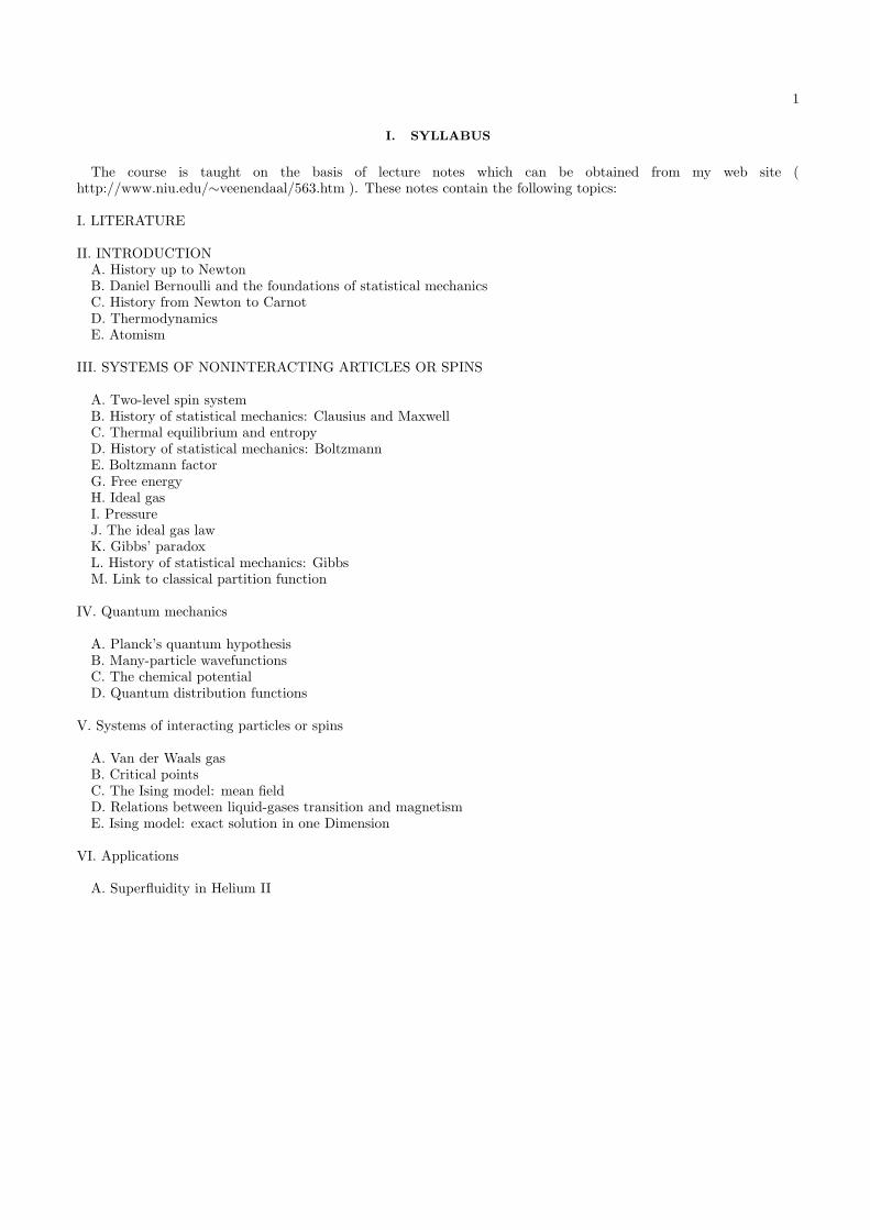
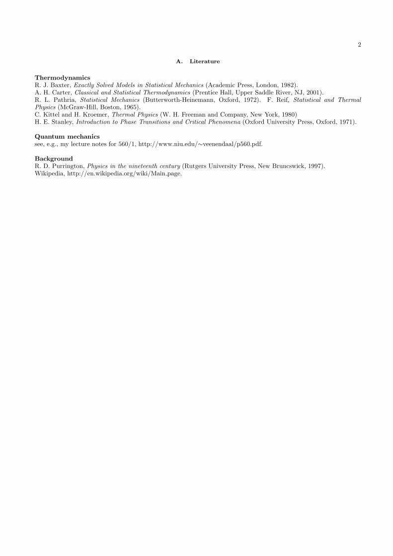
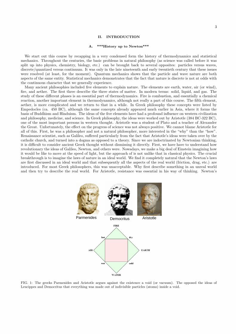
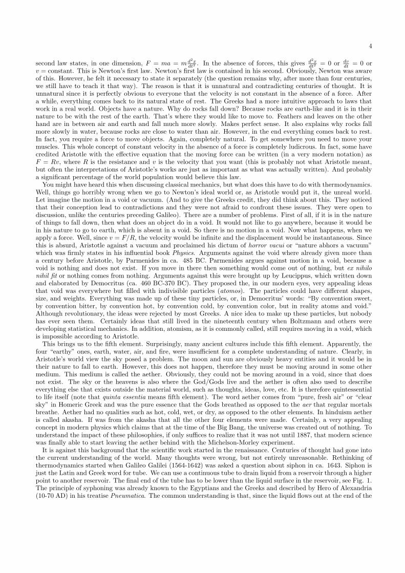
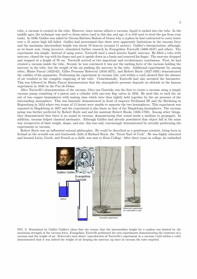

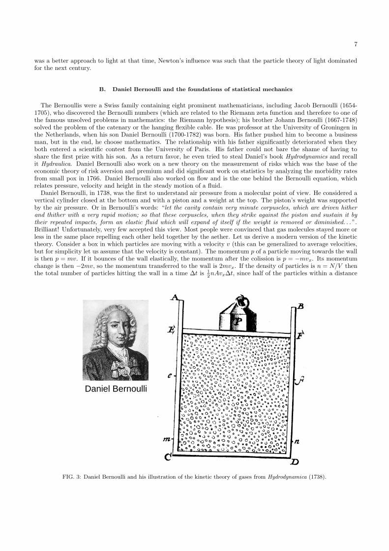
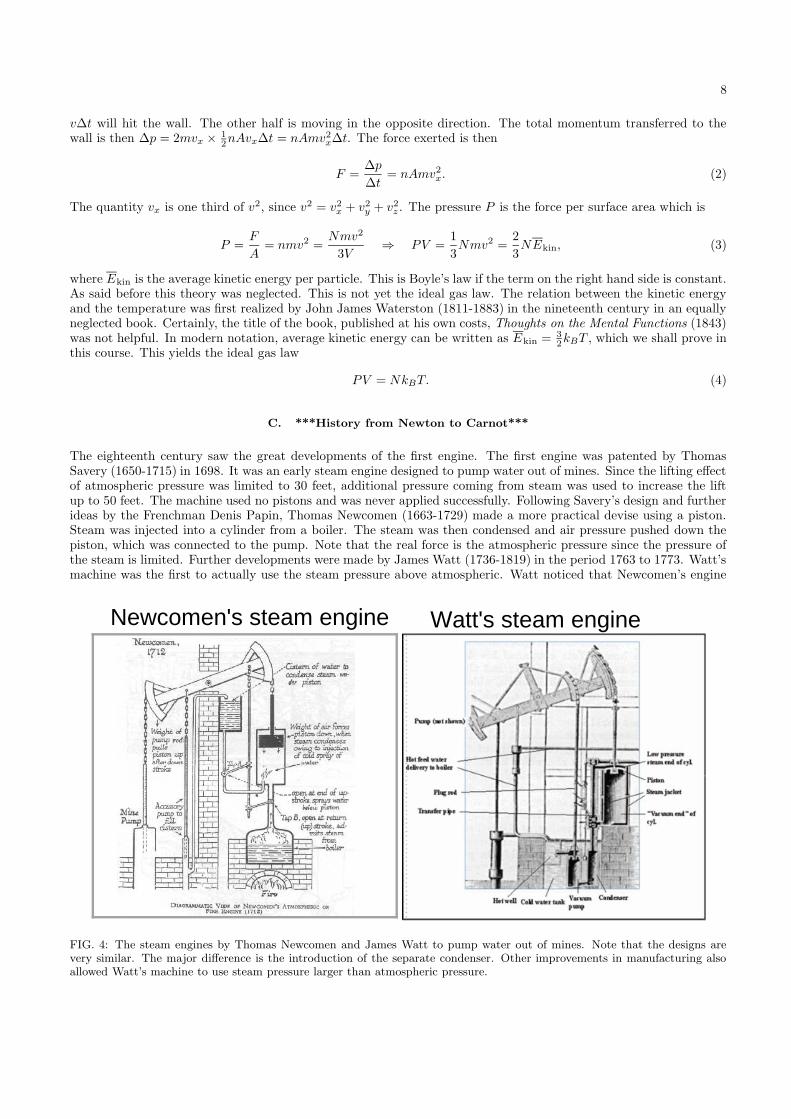
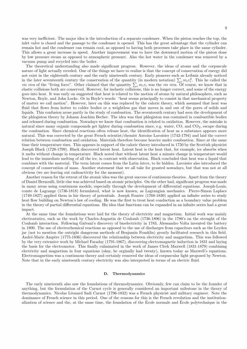

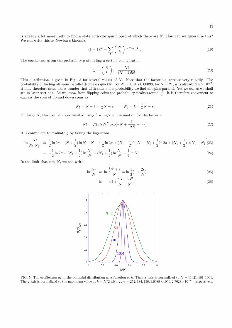
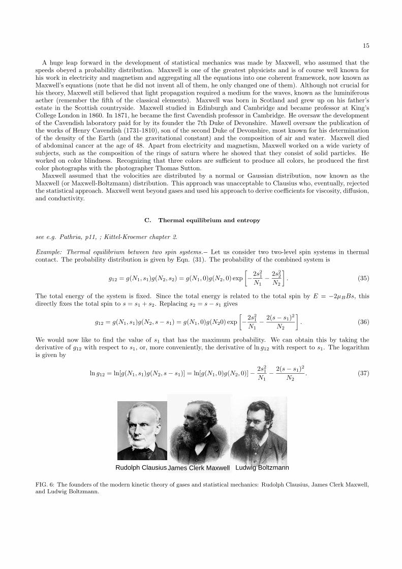
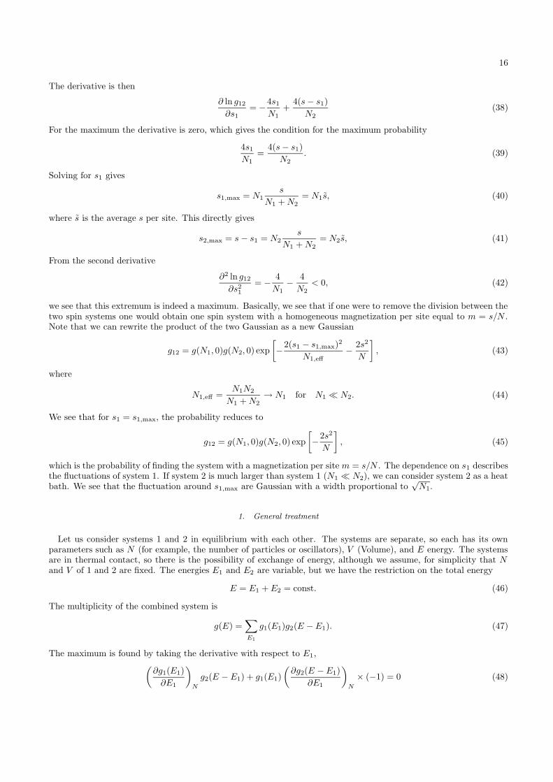
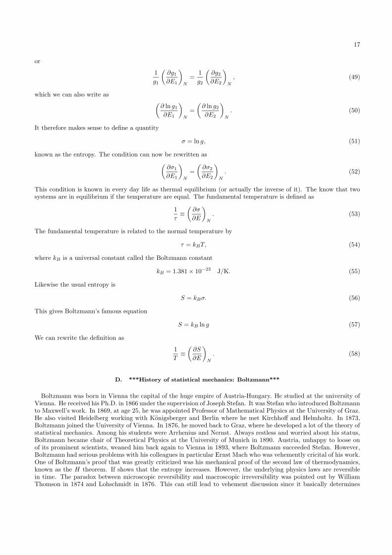

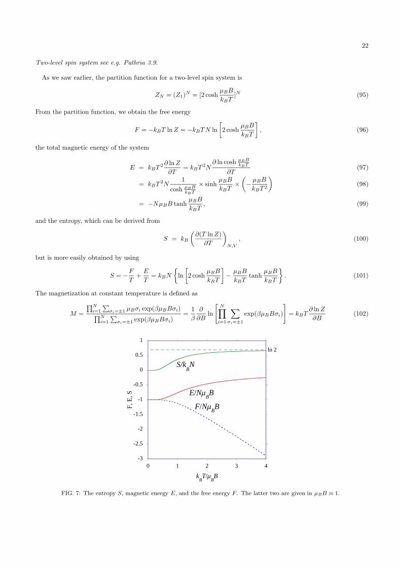


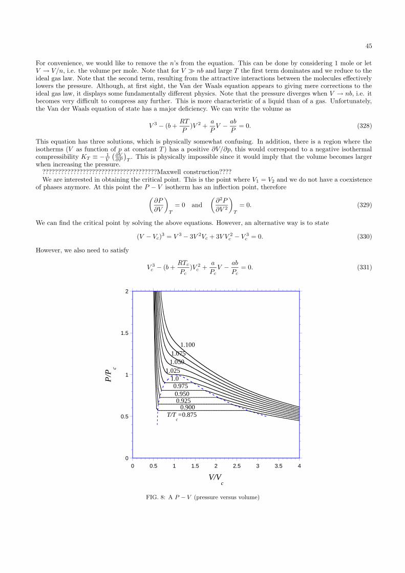
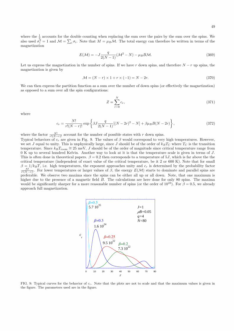
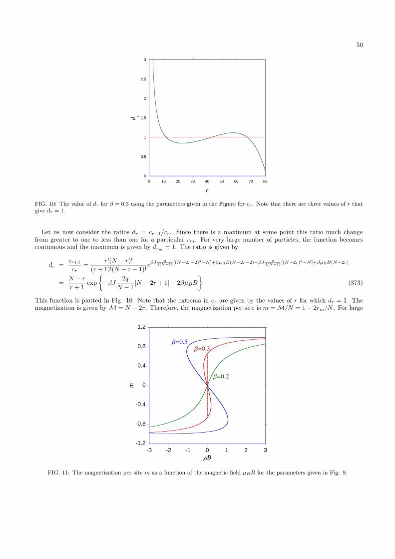
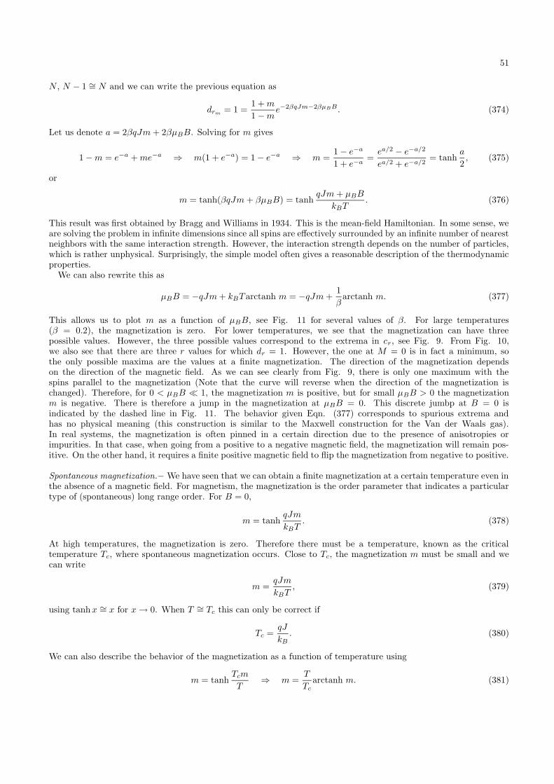

![davcsp.orgdavcsp.org/File/50/Book selling for Class XI _Internal... · 2020-06-12 · Assignment Copy Graph Copy D.A.V. United Magazine TOTAL- OTHER BOOKS Hornbil [English] Snap Shot](https://static.documents.pub/doc/80x56/5f4f59ae2afa395c630350d4/selling-for-class-xi-internal-2020-06-12-assignment-copy-graph-copy-dav.jpg)


![Fire alarm -_internal[1]](https://static.documents.pub/doc/80x56/554e01ccb4c90513298b4999/fire-alarm-internal1.jpg)


