38
I. The Solow model Dynamic Macroeconomic Analysis Universidad Aut´onoma de Madrid Autumn 2014 Dynamic Macroeconomic Analysis (UAM) I. The Solow model Autumn 2014 1 / 38

I. The Solow model
Dynamic Macroeconomic Analysis
Universidad Autonoma de Madrid
Autumn 2014
Dynamic Macroeconomic Analysis (UAM) I. The Solow model Autumn 2014 1 / 38

Objectives
In this first lecture we will study the Solow growth model.
The Solow model is the basis for modern growth theory.
It offers a simplified representation of the mechanics of growth,placing particular emphasis on the role of capital accumulation.
Households own the capital stock and save a fixed proportion of theirincome.
In later themes we will construct a genuine dynamic generalequilibrium models with almost identical predictions.
Dynamic Macroeconomic Analysis (UAM) I. The Solow model Autumn 2014 2 / 38

Proximate vs fundamental causes of growth
The Solow model helps us understand how capital accumulation,population growth and technological change contribute to the growthof living standards.
In the terminology of Acemoglu these are “proximate causes” ofeconomic growth. They fail to explain the persistence of thepronounced differences in living standards.
The study of the “fundamental causes” of these income differences,such as the quality of institutions, is left for future study.
Even so, a thorough understanding of the mechanics of growth isessential.
Dynamic Macroeconomic Analysis (UAM) I. The Solow model Autumn 2014 3 / 38
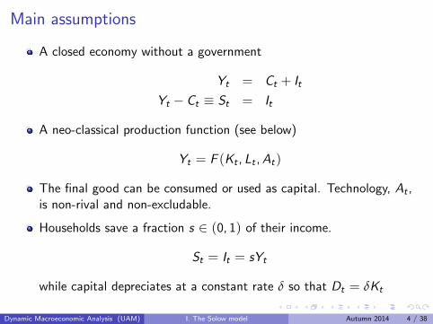
Main assumptions
A closed economy without a government
Yt = Ct + It
Yt − Ct ≡ St = It
A neo-classical production function (see below)
Yt = F (Kt , Lt , At)
The final good can be consumed or used as capital. Technology, At ,is non-rival and non-excludable.
Households save a fraction s ∈ (0, 1) of their income.
St = It = sYt
while capital depreciates at a constant rate δ so that Dt = δKt
Dynamic Macroeconomic Analysis (UAM) I. The Solow model Autumn 2014 4 / 38
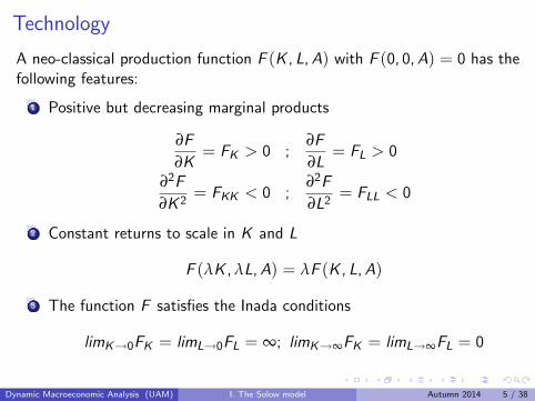
Technology
A neo-classical production function F (K , L, A) with F (0, 0, A) = 0 has thefollowing features:
1 Positive but decreasing marginal products
∂F
∂K= FK > 0 ;
∂F
∂L= FL > 0
∂2F
∂K 2= FKK < 0 ;
∂2F
∂L2= FLL < 0
2 Constant returns to scale in K and L
F (λK , λL, A) = λF (K , L, A)
3 The function F satisfies the Inada conditions
limK→0FK = limL→0FL = ∞; limK→∞FK = limL→∞FL = 0
Dynamic Macroeconomic Analysis (UAM) I. The Solow model Autumn 2014 5 / 38
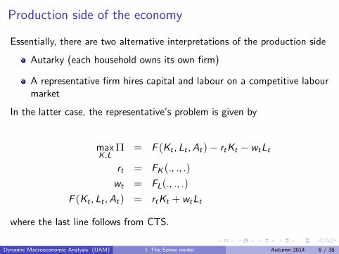
Production side of the economy
Essentially, there are two alternative interpretations of the production side
Autarky (each household owns its own firm)
A representative firm hires capital and labour on a competitive labourmarket
In the latter case, the representative’s problem is given by
maxK ,L
Π = F (Kt , Lt , At)− rtKt − wtLt
rt = FK (., ., .)wt = FL(., ., .)
F (Kt , Lt , At) = rtKt + wtLt
where the last line follows from CTS.
Dynamic Macroeconomic Analysis (UAM) I. The Solow model Autumn 2014 6 / 38
Continuous time
For convenience we analyze the model in continuous time
The instantaneous change in any variable Xt is denoted by
Xt =dXt
dt
(= lim∆→0
Xt+∆ − Xt
∆
)
Dynamic Macroeconomic Analysis (UAM) I. The Solow model Autumn 2014 7 / 38

Law of motion of the capital stock
The change in the capital stock at t, Kt , is the difference between grossinvestment It , and depreciation, Dt :
Kt = It −Dt
= sYt −Kt
= sF (Kt , Lt , At)− δKt
Dynamic Macroeconomic Analysis (UAM) I. The Solow model Autumn 2014 8 / 38
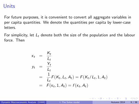
Units
For future purposes, it is convenient to convert all aggregate variables inper capita quantities. We denote the quantities per capita by lower-caseletters.
For simplicity, let Lt denote both the size of the population and the labourforce. Then
κt =Kt
Lt
yt =Yt
Lt
=1
LtF (Kt , Lt , At) = F (Kt/Lt , 1, At)
= F (κt , 1, At) = f (κt , At)
Dynamic Macroeconomic Analysis (UAM) I. The Solow model Autumn 2014 9 / 38

Benchmark
In our benchmark, we abstract from population growth or technicalprogress. So,
Lt = L
At = A
while
κt =δ
δt
(Kt
L
)=
LKt −Kt0
L2=
Kt
L
Dynamic Macroeconomic Analysis (UAM) I. The Solow model Autumn 2014 10 / 38
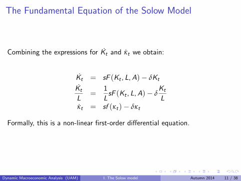
The Fundamental Equation of the Solow Model
Combining the expressions for Kt and κt we obtain:
Kt = sF (Kt , L, A)− δKt
Kt
L=
1
LsF (Kt , L, A)− δ
Kt
Lκt = sf (κt)− δκt
Formally, this is a non-linear first-order differential equation.
Dynamic Macroeconomic Analysis (UAM) I. The Solow model Autumn 2014 11 / 38

Example: Cobb-Douglas production function
The Cobb-Douglas production function is a convenient example of aneo-classical production function:
Y = AK αL1−α
y =AK αL1−α
L= AK αL−α
= Aκα = f (κ, A)
The function f (., .) is a strictly concave function of κ with
δf (κ, A)δκ
= f ′(κ, A) = αAκα−1 =αA
κ1−α
limκ→0f ′(κ, A) = ∞limκ→∞f ′(κ, A) = 0
Dynamic Macroeconomic Analysis (UAM) I. The Solow model Autumn 2014 12 / 38
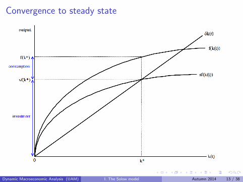
Convergence to steady state
Dynamic Macroeconomic Analysis (UAM) I. The Solow model Autumn 2014 13 / 38
Convergence to steady state
The previous slide has demonstrated that the economy converges(monotonically) to a steady state with κt = κ∗.
The economy replicates itself because each agent (or household) saves aquantity i∗ = sf (κ∗) that exactly compensates for the depreciation of hercapital d∗ = δκ∗.
Formally, for any initial capital stock κ0 ∈ (0, κ∗) the economy willexperience a period of growth in which κt and yt are strictly positive.
Once the economy reaches the steady state, growth comes to an end.
Note, convergence to k∗ will occur for any κ > 0, including the cases inwhich the economy starts out with a κ0 > κ∗ (see below).
Dynamic Macroeconomic Analysis (UAM) I. The Solow model Autumn 2014 14 / 38
What guarantees convergence?
The assumption of a neo-classical production technology is a sufficientcondition to guarantee convergence to a unique steady state:
The Inada condition limK→0FK = ∞ guarantees that the curve sf (κ)is steeper than δκ near the origin;
The diminishing marginal returns to capital guarantee that sf (κ) is astrictly concave function;
The second Inada condition, limK→∞FK = 0, guarantees that thecurve sf (κ) intersects deltaκ for some finite κ.
The intersection is unique because the slope of sf (κ) is a strictlydecreasing function of κ.
Dynamic Macroeconomic Analysis (UAM) I. The Solow model Autumn 2014 15 / 38
Relevant features of the steady state
Our assumptions about technology guarantee that there is a uniquesteady state with a positive capital-labour ratio κ∗.
There is also a trivial steady state with κ∗ equal to zero, but we willignore this unstable steady state.
It is common to talk about steady-state equilibria. But formally theentire trajectory from κ0 to κ∗ should be part of any equilibriumdefinition.
The unique positive levels of κ∗ and y ∗ are strictly increasing in s andA, and decreasing in δ.
By contrast, consumption per capita, c∗, is increasing in A butnon-monotonic in s (lims→0c∗ = lims→1c∗ = 0).
Dynamic Macroeconomic Analysis (UAM) I. The Solow model Autumn 2014 16 / 38
The Golden Rule
We cannot perform a formal welfare analysis as we have not specifiedagents’ preferences over consumption and labour.
Nonetheless, we can ask ourselves whether the steady-state allocationgenerates the maximum feasible level of steady-state consumption.
In any steady state, i∗ = It/L = δκ∗ . Since c∗ = f (κ∗)− i∗ we cantherefore define the golden-rule capital stock as
argmaxκc∗ = f (κ∗)− δκ∗
The FOC that implicitly defines κgold is:
f ′(κgold ) = δ
Let sgold denote the savings rate required to attain a steady state withκgold . There are no forces in the model to guarantee that s = sgold .
Dynamic Macroeconomic Analysis (UAM) I. The Solow model Autumn 2014 17 / 38

Steady-state consumption and the Golden Rule
Dynamic Macroeconomic Analysis (UAM) I. The Solow model Autumn 2014 18 / 38

Dynamic inefficiency
The concept of the Golden Rule is not just useful to identify the allocationwith the highest steady-state consumption level. It also allows us torecognize inefficient allocations.
In particular, any steady state with κ∗ > κgold (or s > sgold) is inefficient.
If the agents were to reduce their savings rate to sgold consumption willconverge to the maximum level cgold . And along the transition to steadystate the agents will enjoy even higher consumption levels.
In other words, if agents value consumption they must be unambiguouslybetter off than under the initial steady state.
Dynamic Macroeconomic Analysis (UAM) I. The Solow model Autumn 2014 19 / 38

Intertemporal tradeoffs
Now suppose the economy is located in a steady state with κ∗ < κgold
(and s < sgold). Once more c∗ < cgold , but this time we cannot makeunambiguous efficiency statements.
To reach the Golden Rule capital stock, the agents have to raise theirsavings rate. This generates an immediate reduction in consumption fromc∗ = (1− s)f (κ∗) to c ′ = (1− sgold )f (κ∗).
Consumption will grow over time and will eventually exceed c∗.
In other words, the agents have to trade off lower consumption todayagainst higher consumption in the future. A formal analysis of the welfareconsequences requires a fully specified model with preferences.
Dynamic Macroeconomic Analysis (UAM) I. The Solow model Autumn 2014 20 / 38
Population growth
Once we allow for population growth, the economy converges to a steadystate in which all aggregate variables grow at the same rate as Lt , butagain there is no growth in per capita variables.
Constant population growth
Lt
Lt= n
κt =δ
δt
(Kt
Lt
)=
LtKt −Kt Lt
L2t
=Kt
Lt− κt
(Lt
Lt
)=
Kt
Lt− κtn
Dynamic Macroeconomic Analysis (UAM) I. The Solow model Autumn 2014 21 / 38
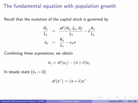
The fundamental equation with population growth
Recall that the evolution of the capital stock is governed by
Kt
Lt=
sF (Kt , Lt , A)Lt
− δKt
Lt
κt =Kt
Lt− κtn
Combining these expressions, we obtain
κt = sf (κt)− (n + δ)κt
In steady state (κt = 0)
sf (κ∗) = (n + δ)κ∗
Dynamic Macroeconomic Analysis (UAM) I. The Solow model Autumn 2014 22 / 38
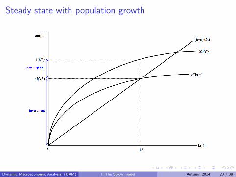
Steady state with population growth
Dynamic Macroeconomic Analysis (UAM) I. The Solow model Autumn 2014 23 / 38
Characteristics of the steady state
In steady state all per capita variables, such as κt , yt , it or ct , remainconstant over time.
By contrast, all aggregate variables grow at the same rate as thepopulation. For example,
Kt = κ∗Lt
log(Kt) = log(κ∗) + log(Lt)
Taking derivatives with respect to t yields
Kt
Kt= 0 +
Lt
Lt= n
From CRTS, it follows that Yt and hence Ct and It also grow at rate n.
Dynamic Macroeconomic Analysis (UAM) I. The Solow model Autumn 2014 24 / 38
Transitional dynamics
Since yt is stricly increasing in κt , the growth rate of y (yt/t) isproportional to the growth rate of κ
γκ ≡κ
κ= s
f (κ, A)κ− (n + δ)
The concavity of f (., .) implies that the average output per unit of capitalis decreasing in κ.
Hence the growth rate of κ is strictly decreasing in κ with γκ > 0 for allκt < κ∗ and γκ < 0 for κt > κ∗. This combined withlimκ→0(f (κ, A)/κ) = ∞ guarantees existence and uniqueness.
Dynamic Macroeconomic Analysis (UAM) I. The Solow model Autumn 2014 25 / 38

Growth and convergence
Correct interpretation: g=0
Dynamic Macroeconomic Analysis (UAM) I. The Solow model Autumn 2014 26 / 38

Technological progress
In the basic Solow model we can only have sustained growth if there issustained technological progress. Moreover, balanced growth is onlypossible if technological progress is labour-augmenting. Formally, we will
assume
Yt = F (Kt , AtLt)At
At= x
Next, we let Lt = AtLt denote the efficiency units of labour and
κt =Kt
Lt
=Kt
AtLt
yt =F (Kt , Lt)
Lt
= f (κt)
Dynamic Macroeconomic Analysis (UAM) I. The Solow model Autumn 2014 27 / 38

Balanced growth with exogenous technological change
Following the same procedure like before, we arrive at
δ
δt
(Kt
AtLt
)=
Kt
Lt
− κt(x + n)
Kt
Lt
= sf (κt)− δκt
Combing the above equations we arrive at the fundamental equation withtechnological growth
δκt
δt= sf (κt)− (n + δ + x)κt
Dynamic Macroeconomic Analysis (UAM) I. The Solow model Autumn 2014 28 / 38

Interpretation of the balanced growth path
Once the economy reaches the steady state,
All quantities per efficiency unit (y , c and κ) are constant over time
All quantities per capita (y , c and κ) grow at the rate n.
All aggregate variables (Y , C and K ) grow at the rate n + x .
However, it should be reminded that the growth of At is generatedexogenously. Eventually, we would like to understand the drivers behindtechnological progress (investments in human capital, R&D, etc. ).
In order to generate endogenous growth with investment in R&D we needto abandon the assumption of perfect competition.
Dynamic Macroeconomic Analysis (UAM) I. The Solow model Autumn 2014 29 / 38
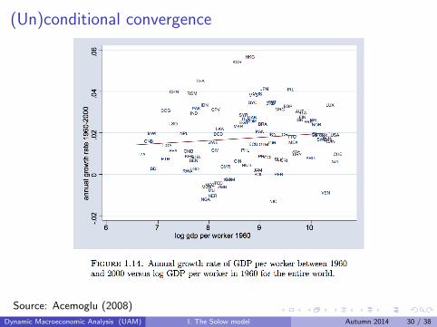
(Un)conditional convergence
Source: Acemoglu (2008)
Dynamic Macroeconomic Analysis (UAM) I. The Solow model Autumn 2014 30 / 38

(Un)conditional convergence
Source: Acemoglu (2008)
Dynamic Macroeconomic Analysis (UAM) I. The Solow model Autumn 2014 31 / 38
Conditional convergence
The model predicts that the growth rate of capital and income per capitaare falling in the level of capital. Hence, if the level of capital is the ONLYdifference between two countries, then:
The poor country should grow at a faster rate than the rich country
Both countries should eventually converge to the same steady state.
The conditional convergence of income levels is a prediction of the modelthat is verified by the data.
Similarly, nothing prevents the divergence between countries with differentfundamentals.
Dynamic Macroeconomic Analysis (UAM) I. The Solow model Autumn 2014 32 / 38
Decentralized equilibrium
So far we have abstracted from markets, assuming that agentsoperate a backyard technology.
It is straightforward to relax this assumption and assume thathouseholds offer their capital and labour services on competitivemarkets
The representative firm maximizes profits so that
wt = FL(Kt , Lt)Rt = FK (Kt , Lt)
All factor markets clear at all dates
Dynamic Macroeconomic Analysis (UAM) I. The Solow model Autumn 2014 33 / 38
Equilibrium
Consider the version with population growth:
For a given sequence of {L(t), At}∞t=0 and and initial capital stock K0 an
equilibrium path is a sequence of capital stocks, output levels, consumptionlevels, wage rates and rental prices {Kt , Yt , Ct , wt , Rt}∞
t=0 such that
Kt = sF (At , Kt , Lt)− (n + δ)Yt = F (At , Kt , Lt)Ct = (1− s)Yt
Rt = FK () = f ′(κt)wt = FL() = f (κt)− f ′(κt)
Dynamic Macroeconomic Analysis (UAM) I. The Solow model Autumn 2014 34 / 38

Dynamic inefficiency
In this economy, the agents receive steady state net-interest rater ∗ = R∗ − δ = f ′(κ∗)− δ.
The Golden Rule capital stock is defined by f ′(κGOLD) = n + δ
Thus for dynamically inefficient allocations with k∗ > kGOLD , it musttrue that
f ′(κ∗) = r ∗ + n < n + δ
r ∗ < n
In later themes we will see that this condition implies that a PAYGOpension scheme improves welfare
Dynamic Macroeconomic Analysis (UAM) I. The Solow model Autumn 2014 35 / 38
Sustained growth — The AK model
In order to generate sustained growth without exogenous technologicalchange, we need to relax some of the assumptions of the Solow model.
A logical candidate is to consider alternatives to the assumption of aneo-classical production technology
In the Solow model growth vanishes due to the decreasing marginalproduct of capital
We can show that perpetual growth is feasible if output is linear in Kso that
Yt = AKt
This interpretation is acceptable if we use a broad concept of capitalthat includes both human and physical capital.
Dynamic Macroeconomic Analysis (UAM) I. The Solow model Autumn 2014 36 / 38
Sustained growth — The AK model
In the AK -model, per capita output is equal to y = AK /L = Aκ. In otherwords, the fundamental equation remains valid
κ = sy − (n + δ)κ
= sAκ − (n + δ)κ
and so the growth rate of κ can be written as
κ
κ= sA− (n + δ)
which is constant and independent of κ.
Dynamic Macroeconomic Analysis (UAM) I. The Solow model Autumn 2014 37 / 38
Distinctive features of the AK model
1 The model produces sustained growth without sustained growth in anexogenous variable like A
2 The growth rate is increasing in the savings rate
3 No transitional dynamics — the growth rate is constant and equal tosA− (n + δ)
4 No convergence
5 Recessions produce permanent effects on living conditions
6 The economy is never dynamically inefficient
Dynamic Macroeconomic Analysis (UAM) I. The Solow model Autumn 2014 38 / 38


