Master’s Degree in Economics and Finance Final Thesis IAG Company’s Optimal Capital Structure reached through a Multi-objective Genetic Algorithm Supervisor Ch. Prof. Marco Corazza Graduand Andrea Barison Matriculation number 867886 Academic Year 2018 / 2019
Transcript
Master’s Degree
in Economics and Finance
Final Thesis
IAG Company’s Optimal Capital Structure reached through a
Multi-objective Genetic Algorithm
Supervisor Ch. Prof. Marco Corazza
Graduand Andrea Barison Matriculation number 867886
Academic Year
2018 / 2019
If you don't go after what you want, you will never have
it. If you don't ask, the answer will always be no. If you
don't step forward, you will always be in the same place.
N. R.
Acknowledgments
First of all, I sincerely thank my supervisor, professor Marco Corazza for all the advices
and support he gave me whenever I had doubts during this thesis writing.
Besides my supervisor, I would like to thank two of my University colleagues, with
whom I shared this 2-years journey. Chiara and Andrea, without you it would not have
been the same! I found two real and always helpful friends.
I owe my deepest gratitude to my parents Roberta and Massimo and my brother
Alessandro, who always believed in me and supported me when I needed it.
Especially, I would like to thank my girlfriend, Eleonora, for all her love and patience.
Last but not least, I want to thank all my friends and peers too. A special thank you
goes to Rocco and Enrico who always encouraged me for the next steps of my working
When it comes to making decisions in a business, the general objective of Corporate
Finance is the maximization of the firm’s value. Therefore, to assess the performance
of the company in general, managers and stockholders need evaluation techniques
which allow to address also the potential conflict between them. In this respect, the
predominant purpose of Corporate Governance is the attempt at “balancing the
interests of power between the different stakeholders by management control,
regulation of market discipline and transparency and quality of corporate disclosure”1.
The maximization of the firm’s value is usually reached by adjusting the principal
components of the company’s capital structure2 with the final aim of optimizing it.
Companies always try to operate in an optimum range of capital structure and “if they
have to be excluded from this optimized range due to business conditions, they will
return as soon as possible”3. In such context, indeed, most of the economics books
describe the structure parameter as the most effective parameter for the evaluation of
companies operating in Capital markets.
Regarding the study of an optimal capital structure, several theories have been
provided both by researchers and financial managers and its assessment dates back in
late 1950s with the Modigliani and Miller Theory (1958), among the others: Jensen and
Meckling with the Static Trade-Off Theory (1976) and the Agency Cost Theory (1976),
Myers with the Pecking Order Theory of Financing Choice (1984), Jensen with the Free
Cash Flow Hypothesis (1986), Baum and Crosby with the NOI (Net Operating Income)
Approach (1988), Mundy with NI (Net Income) Approach (1992), Baker and Wurgler
with Market Timing Theory (2002) and more dynamic Trade-off Models such as the
ones proposed by Brennan and Schwartz (1984).
1 ECB. (2015). The evolving framework for corporate governance. Monthly Bulletin. May 2005, pages 88-90. 2 The Capital Structure is defined as the firms’ combination of different securities (Debt, Equity and mixes of the two), used to finance their projects and, more generally, all their operations and growth. 3 MUELLER, E., SPITZ, A. (2006). Managerial ownership and company performance in German small and medium-sized private enterprises. German Economic Review. 2, pages 2-18.
4
These various capital structure theories try to establish a relationship between the
financial leverage of a company (i.e., the proportion of debt in the company’s capital
structure) with its market value. Although these theories provide different financing
methods (behaving as it is shown in Table 0.1), the results are controversial, and no
one seems, actually, to provide a real optimized model. Table 0.1 summarizes all the
previously mentioned theories and, for each one, compares the relative effects on:
Leverage (L), Cost of Capital (K), and Expected Return (R) with respect to the final
Value (V) of the company under analysis. In the table the symbol ↑ stands for
increase, while ↓ stands for decrease.
Theory /
Approach Effect (1) Effect (2) Results
Net Income
Approach (NI) L↑
K↓
P↑ V↑
Net Operating
Income Approach
(NOI)
L↑ K V
Modigliani & Miller
Theory (Non-debt
tax shield)
L↑ K↑
R↑ V↓
Modigliani & Miller
Theory (Debt tax
shield)
L↑ K↓ V↓
Static Trade Off
Theory L↑
K↓
Financial
Distress ↑
V↑
5
Pecking Order
Theory
First internal sources,
then external sources ↑
Endeavor to
invest on
positive net
present
value
projects ↑
First benefit
for present
shareholders,
then an
opportunity
for new
investors ↑
Agency Cost Theory
Conflict of interest
between management,
shareholders and
creditors ↑
----- V↓
Conflict of interest
between management,
shareholders and
creditors ↓
----- V↑
Free Cash Flow
Hypothesis
L↑
Dividend ↑
Agency Cost
↓ V↑
Dynamic Trade Off
Theory
Correct future
forecasting ↑ ----- V↑
Incorrect future
forecasting ↑ ----- V↓
Market Timing
Theory
Overvalue of shares ↑ Issuing new
shares V↑
Undervalue of shares ↑ Buyback
their shares V↑
Table 0.1: Theories and approaches of Capital Structure
*Source: AFRASABI, J., AHMADINIA, H., HESAMI, E. (2012). A Comprehensive Review on
Capital Structure Theories. The Romanian Economic Journal. Vol XV(45).
6
Furthermore, since the determination of the optimal capital structure belongs to the
family of the prescriptive theories (we are looking for a target debt ratio in order to
find the optimal mix of debt and equity that is applicable in the real world) and since it
is based on the partial equilibrium4, other researchers tried to develop new theories
and/or to assess the target debt-equity ratio through new determinants.
Due to the deficiencies of traditional methods, as highlighted by the controversial
results in the above Table, this thesis aims at providing a model that works on a proper
mix of debt and equity such that it is possible to reach the optimal capital structure
with some pre-determined specific objectives. Indeed, the proposed model is drawn
considering the profitability maximization (from the equity holder’s point of view),
meanwhile keeping a proper level of debt repayment ability, in order to better balance
the interests of the company’s shareholders and the ones of the debt-holders.
In investment analysis the use of accounting measures of return, such as Return on
Equity (ROE) or Return on Capital (ROC), still continue to prevail (partially because of
their intuitive appeal for both investors and analysts, and partially because financial
managers are reluctant to abandon familiar measures). However, here, the model is
implemented through the use of the Genetic Algorithms (GAs) specific research
technique, which is a trial-and-error stochastic search optimization algorithm used to
solve complex optimization problems. In other words, GAs is a method for
optimization and it can utilize as variables these kind of accounting measures. The
choice of this specific search-metaheuristic, inspired by Charles Darwin’s theory of
natural evolution, comes from various reasons such as its ease of implementation (GA
indeed provides a problem-independent method for solution searching), its
equilibrium between exploration and exploitation5 (achieved by the proper setting of
the parameters) and, in addition, because it is one of the pioneer evolutionary
algorithms and uses a mathematical and logical reasoning which allows GA to be
4 Partial equilibrium is a condition that takes into account the impact only of a part of the market variables to reach equilibrium, ignoring therefore secondary variables (i.e., the ones which are assumed to have a small or null impact in any other market). 5 Exploration focuses on the research of current good solutions in a local region, instead the exploitation generates different solutions in order to explore the search space on a global scale.
7
applied to different types of optimization problems in any field. Furthermore, Genetic
Algorithm has stood out for its strong robustness and good convergence6.
Corporate financial theory is primarily focused on stock price maximization, mainly
because stock prices are constantly updated perceivable measures that could be used
to evaluate the performances of firms and because, if investors were rational and
markets efficient, stock price would reflect the long-term effects of the firms’ choices
(regarding for example the pick-up of specific projects or the way in which these
projects are financed). However, are we sure that the aggregation of rational
individuals creates a “rational” environment? Every economics’ concept starts from
the assumption that the economic agents behave rationally. Interestingly, a singular
agent behaviour can be defined as rational, even if sometimes he/she takes some non-
rational decision. But what happens if many agents take non-optimal and non-fully
utility-maximizing decisions simultaneously? More often than we might think, this
happens in the financial markets.
If we want to start from the assumption of markets following non-predictable
movements (random patterns), an interesting suitable approach could be the
implementation of a Genetic Algorithm model, since it is an optimization algorithm
that starts from a batch of random solutions as well. The algorithm firstly finds the
answer between random potential solutions (called chromosomes) through the basic
operations of selection, crossover and mutation, then gradually improves the fitness
function of the offspring7, which gradually gets better than the one of the parents, and
ultimately gets the optimal solution for the problem. The Genetic Algorithm stem,
indeed, from the Darwinian idea of the “survival of the fittest” (natural system which
follows the natural pattern of growth and reproduction).
6 For more information, see: IYER, K. C., SAGHEER, M. (2012). Optimization of bid-winning potential and capital structure for build-operate-transfer road projects in India. Journal of Management in Engineering. 28(2), pages 104–113. 7 The fitness function represents the score assigned to each point (i.e., solution) of the offspring generation, that is the transformation (through the selection, crossover and mutation operators) of the old generation into the new one.
8
This application of the GA in order to find the optimal capital structure will be
performed to the specific case study of International Consolidated Airlines Group S.A.
(aka IAG). IAG is a publicly traded holding company born out in 2011 from the merge of
the UK’s largest airlines company British Airways (aka BA) and the Spanish airlines
company Iberia, joined later also by the Spanish company Vueling Airlines in 2013. IAG
Company provides transportation services, offering both domestic and international
air passenger and cargo transportations.
9
CHAPTER 1
Firms’ Capital Structure
The Capital Structure of a company represents the way the company
finances its assets. In this first chapter, the commonly pursued
objective of firms is introduced and explained through the estimation
of the Cost of Capital. The Cost of Capital is then split and analysed
across all of its components.
1.1 The classic businesses’ objective
In the corporate finance field, the classical objective among firms is the value
maximization. There are although some disagreements whether this maximization
should be meant from the point of view of the stockholders or from the point of view
of the firm (which includes not only the stockholders but all stakeholders and the
other financial claim holders like debt holders who bought some bonds issued by the
company). The optimal or target capital structure is the one which simultaneously
maximizes the firm value, minimizes the weighted average cost of capital and
maximizes the market value of its stock. The goal of managing capital structure is
maximizing the value of the firm.
Since the decisions in a business are generally taken by managers, rather than the
owners, they will decide the way in which raising new funds for investments and,
therefore, where to invest. Here comes the point. If the objective is stated in terms of
stock price maximization, the managers will take the choice among different
10
alternatives and the way to pick projects analysing which one will increase the stock
price more.
The main reasons to choose as objective solely the stock price maximization are:
➢ They reflect the long-term effects of the choices taken by the firm, since they
are a function not only of current operations (which can be analysed simply
looking at the financial statement or other accounting measures) but also of
the future chances of success and stability;
➢ They are a clear target for mangers and they could be seen as a proxy of the
performance of publicly traded firms;
➢ They are constantly updated and always observable. Looking at their trend,
managers could extrapolate the feelings of the investors regarding their
choices. In other words, they can be seen as investors’ feedbacks.
Focusing solely on the narrower objective of stock price maximization, with respect to
the firm value maximization, we are implicitly assuming that stock prices are
reasonable and unbiased estimates of the real value of that firm.
Indeed, the primary goal of financial managers is the maximization of stockholders’
wealth, and this is reached by maximizing the value of the firm (or, equivalently,
minimizing the WACC). Why is it equivalent to talk about maximizing the value of the
firm and minimizing the Weighted Average Cost of Capital? Since the WACC is
considered the most appropriate discount rate for the risk of the firm’s assets, we can
use it to get the firm’s value by discounting its expected future cash flows. Firm value
will be therefore maximized when the WACC is minimized, since value and discount
rates move in opposite directions.
11
1.2 Estimation of the Cost of Capital
The Cost of Capital is the cost of a company’s funds and it is commonly defined as the
minimum required rate of return (also known as hurdle rate) that a firm must earn on
its investments (assets) to satisfy its owners, the creditors and the other providers of
capital, or they will invest elsewhere. Indeed, investors (who provide capital to the
companies) consider an investment worthwhile if the expected Return on Capital (RoC)
is higher than the Cost of Capital.
This concept is a basic input information in capital investment decision and its
importance encompasses different managerial decisions such as:
➢ Capital Budgeting Decisions (the firm invests in projects that provides a
satisfactory return, at least greater than the Cost of Capital of that project. In
other words, there is a settlement of a benchmark that a new project has to
meet)
➢ Corporate Financial Structure Design (managers need to change the methods
of financing in order to increase the market price and the EPS – Earnings per
Share. To maximize its value, the firm should minimize the cost of all its
inputs)
➢ Management Performance Measures (financial performances could be
evaluated through a comparison of the profitability of the projects with the
planned overall cost of capital)
➢ Others (dividend decisions, working capital policy, bond refunding etc.)
In addition, the Weighted Average Cost of Capital (WACC) can be used by investors to
choose the best corporate-investments and to calculate Discounted Cash Flow (DCF)
valuation of companies. Indeed, “the most widely used technique for financial
12
evaluation is discounting the cash flow by weighted average cost of capital both in
literature and practice”8.
Aswath Damodaran, professor of Corporate Finance and Valuation at the Stern School
of Business at New York University, wrote in his book Applied Corporate Finance: “The
cost of capital is the weighted average of the costs of the different components of
financing (equity, debt and hybrid securities) used by a firm to fund its financial
requirements”9. Therefore, to compute the firm’s Weighted Average Cost of Capital,
one has to estimate the costs of individual financing sources and the market value
weights of each of the components. Companies try to keep the share of the sources of
financing in optimal proportions. The formula can be written as follows:
𝑊𝐴𝐶𝐶 = 𝐾𝐸 ∗ [𝐸
𝐷 + 𝐸 + 𝑃𝑆] + 𝐾𝐷 ∗ [
𝐷
𝐷 + 𝐸 + 𝑃𝑆] + 𝐾𝑃𝑆 ∗ [
𝑃𝑆
𝐷 + 𝐸 + 𝑃𝑆]
where:
E, D, PS stand for Equity, Debt and Preferred Stock, respectively (book values);
𝐾𝐸 , 𝐾𝐷 , 𝐾𝑃𝑆 stand for Cost of Equity, Cost of Debt and Cost of Preferred Stock,
respectively.
Affecting the Cost of Capital there are, however, some factors over which the
companies have no control. These are, for example, the level of interest rates (which
affect the Cost of Debt and, potentially, the Cost of Equity) and the tax rates (which
affect the after-tax Cost of Debt). Companies will work therefore on the maintenance
of the share of the individual components (in other words the sources of financing) in
optimal proportions.
8 BABUSIAUX, D., PIERRU, A. (2001). Capital Budgeting, Investment Project Valuation and Financing Mix: Methodological Proposals. European Journal of Operational Research. 135, pages 325-337.
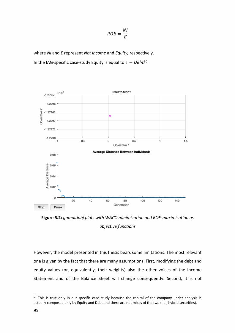
where the % 𝐶ℎ𝑎𝑛𝑔𝑒 𝑖𝑛 𝑜𝑝𝑒𝑟𝑎𝑡𝑖𝑛𝑔 𝑖𝑛𝑐𝑜𝑚𝑒 is usually measured by the EBIT
(Earnings before interest and taxes);
o Degree of financial leverage (a high leverage means high variance in earnings
per share and, therefore, high risk in equity investments in the firm. This
translates in a high beta).
1.3.3.3 Accounting Beta Approach
The third approach (Accounting Beta approach) implies the use of the regression of the
changes in a firm’s earnings against the changes in earnings for the whole market to
21
get an estimate of the market beta for the CAPM formula. Nonetheless, such an
approach presents some drawbacks. Firstly, earnings can be affected by the different
accounting choices. Secondly, the regressions have often not enough observations
since the accounting measures are usually measured just once per year. Lastly, the
accounting earning, compared to the underlying value of the firm, are usually
smoothed out too much.
1.3.4 Cost of Equity Formulation
Recapitulating, now that we have analysed all the determinants, we can get the CAPM
formula for the Cost of Equity which is, as already stated, simply the expected return
from investing in the equity of the firm or, stated in other terms, the rate they require
in order to be compensated for the risk assumed for investing in the equity of the firm.
From mangers’ perspective, the Cost of Equity can be defined as the return they
should manage to reach in order to satisfy the investors.
𝐸𝑥𝑝𝑒𝑐𝑡𝑒𝑑 𝑟𝑒𝑡𝑢𝑟𝑛 = 𝑅𝑖𝑠𝑘 𝑓𝑟𝑒𝑒 𝑟𝑎𝑡𝑒 + 𝐵𝑒𝑡𝑎 ∗ 𝐸𝑅𝑃
When estimating the Cost of Equity using the beta in the CAPM formula as measure of
risk, we implicitly assume that the marginal investor12 is a well-diversified investor.
Nevertheless, in private firms we can not make this assumption (since usually the
owner of a private firms invests the majority of his/her wealth in his own company)
and therefore it is suggested either to add a premium to the Cost of Equity to reflect
the higher risk (given the fact that the investor most probably lacks the possibility to
diversify), either to adjust the beta in order to reflect the total risk (instead of the
market risk only) simply by dividing the market beta by the square root of the R-
12 The marginal investor is an investor who owns a large portion of the equity and trades it frequently and is considered, therefore, to be the investor in the firm who will be the buyer/seller on the upcoming trade.
22
squared statistic, which is a statistic measure of the goodness of fit of the regression
but in this specific economic framework it represents an estimate of the proportion of
the risk that could be imputed to market risk13.
Summarizing, the Return on Equity depends both on business and on financial risk. We
refer to business risk (inherent in the operations of the firm) when it is a risk that
depends on the systematic risk of the assets, while we refer to financial risk when it is
an extra risk to stockholders which results from debt financing and so when it depends
on the level of leverage (Debt/Equity ratio).
There exist, however, other models to calculate the Cost of Equity (depending on the
type of Cost of Equity one wants to consider). One almost equally viable alternative to
the Capital Asset Pricing Model could be represented by the Dividend Capitalization
Model14, which estimates a future dividend stream based on the firm’s dividend
history (assuming a constant growth rate) looking for the market capitalization rate
that match the current market price. To accomplish this, the Dividend Capitalization
Model is based on the following formula:
𝑅𝑒 =𝐷1𝑃0+ 𝑔
where:
𝑅𝑒 is the Cost of Equity;
𝐷1 is the Dividend per share of next period;
𝑃0 is the current share price;
𝑔 is the expected dividend growth rate.
13 Hence, in such an economic framework the (1 − 𝑅2) can be seen as the firm-specific risk. 14 Also called Gordon Growth Model (GGM) from its author Myron J. Gordon who published it along with Eli Shapiro n 1956. To deepen: Gordon, M. J., Eli Shapiro (1956), “Capital Equipment Analysis: The Required Rate of Profit”, Free Press, Management Science, 3(1), 102-110.
23
Since this model is applicable in case of payments of dividends on the shares and
assuming that they will grow at a constant rate, in the case of private firms without
dividends’ distribution, the firm’s ability of apportion of profits through dividends is
assessed looking at the Net Income and cash flows and then compared to the
dividends paid out by firms of analogous dimensions.
Anyway, for the analysis that we are going to perform in the next chapters we will use
the CAPM rather than this Dividend Capitalization Model.
Even if in investment analysis what is commonly used as hurdle rate is the Cost of
Capital, there exist situations in which the use of the Cost of Equity could be more
suitable. For example, if investors want to measure the returns made on their equity
investments (in other words in projects or the entire business of a company) the most
appropriate hurdle rate to consider is the Cost of Equity.
1.4 Cost of Debt
The idea behind comes from the possibility that, when an investor lends to a firm,
there exists the likelihood that the borrower could default on the principal and the
interests of the loan. In such investments (investments with default risk), the risk is
indeed represented by the likelihood that the promised15 cash flows might not be
delivered. Since nothing is to be taken for sure, we should talk about expected return.
The expected return on bonds issued by companies is meant to be the reflection of its
firm-specific default risk. The current cost to the firm of borrowing funds to finance the
projects is commonly known as Cost of Debt. It is a model based on the default risk
and it depends on:
15 It is called promised because investing in bonds issued by a company means that the coupons are fixed at the time of the issue. These coupons are the promised cash flows.
24
➢ Default risk16 of the firm (if it increases, lenders will charge higher interest rates
to reflect the new further risk they are undertaking);
➢ Current level of interest rates (investments with higher default risk should have
higher interest rates and if interest rates rise, the Cost of Debt rises as well. If
interest rates decrease, the Cost of Debt decreases as well);
➢ Tax advantage (since interest is tax-deductible, as tax rates increase, the after-
tax Cost of Debt will be lower than the pre-tax Cost of Debt)
where the default spread is a representation of the default risk of the firm and
it is exactly the premium investors demand over the risk-free rate.
Looking at it from a different perspective, we can say also that borrowers with higher
default risk should pay higher interest rates on their borrowing than those with lower
default risk. With respect to the risk and return models (used in the Cost of Equity)
which assess the effects of the market risk on expected returns, models of default risk
gauge the effects of individual firms’ default risk on pledged returns.
Rating agencies, using a mix of both public and private information (mainly financial
ratios), transform these assessments into measures of default (under the name of
bond ratings), which could be considered by investors as a shorthand measure of
default risk. The two most known and reliable rating agencies are Standard & Poor’s
and Moody’s. In Table 1.1 below it is depicted the way in which they assign these bond
ratings.
16 The default risk is a function of different elements. Firstly, it is function of the firm’s capacity to generate stable cash flows from operations and financial obligations. Secondly, it is function of its assets’ liquidity since it would become easier to liquidate them in crises times when there is the need to meet debt obligations.
25
INDEX OF BOND RATINGS
STANDARD & POOR'S MOODY'S
AAA Highest debt rating assigned.
The borrower's capacity to repay debt is extremely strong
Aaa Best quality with a small
degree of risk
AA Capacity to repay is strong and differs from the highest quality
only by a small amount Aa
High quality but rather than Aaa because margin of
protection may not be as large or because there may be other
elements of long-term risk
A
Strong capacity to repay but the borrower may be
susceptible to adverse effects of changes in circumstances
and economic conditions
A Bonds possess favorable
investment attributes but may be susceptible to risk in future
BBB
Adequate capacity to repay, but adverse economic
conditions or circumstances are more likely to lead to risk
Baa Neither highly protected nor
poorly secured. Adequate payment capacity
BB, B, CCC, CC
Predominantly speculative (BB the least speculative, CC the
most)
Ba Bear some speculative risk.
B Generally lacking features of a
desirable investment, probability of payment small
D In default or with payments in
arrears
Caa Poor standing and perhaps in
default
Ca Very speculative; often in
default
C Highly speculative; in default
Table 1.1: Index of Bond Ratings
26
Ratings range therefore between AAA (or Aaa for Moody’s) to D (or, equivalently, C for
Moody’s), but we can make a division between Investment Grade and Junk Bonds.
Bonds with a rating above BBB (or Baa for Moody’s) are defined as investment grade,
which means there is a very low likelihood of default. On the other hand, bonds with a
rating below that are called junk-bonds or high-yield bonds (since they should promise
high yields, given the risk investors bear lending to the companies that issued them).
Some examples of the financial ratios utilized by the rating agencies to determine
whether the companies are able to meet debt obligations and whether they have
Coverage Ratio, Free Operating Cash Flow over Total Debt, Operating Income over
Sales, Total Debt over Capitalization. Nevertheless, rating agencies do not rely solely
on these financial ratios when assigning grades to a company, but they rather consider
also expectations in future performances (which are kind of subjective evaluations).
Furthermore, the default risk determines the level of the interest rate on corporate
bonds (high rated bonds should yield lower interest rates with respect to lower rated
ones). The default spread is function of the interest rates in the sense that it is
computed as the difference between the interest rate on a corporate bond (bearing
some kind of default risk) and a default-free government bond. This is displayed in
Table 1.2.
The default spread is itself function of the bond’s maturity (showing evidence that
short-term default risk is greater than long-term default-risk) and of economic
conditions (revealing that default spreads increase during economic slowdowns). This
implies a drawback: default spreads for bonds must be re-evaluated quite often.
Rating is:
Spread
2018
Spread
2017
Spread
2016
Spread
2015
Interest rate
on bond
Aaa/AAA 0,54% 0,60% 0,75% 0,40% 2,95%
Aa2/AA 0,72% 0,80% 1,00% 0,70%
A1/A+ 0,90% 1,00% 1,10% 0,90%
27
A2/A 0,99% 1,10% 1,25% 1,00% 3,34%
A3/A- 1,13% 1,25% 1,75% 1,20%
Baa2/BBB 1,27% 1,60% 2,25% 1,75% 3,68%
Ba1/BB+ 1,98% 2,50% 3,25% 2,75%
Ba2/BB 2,38% 3,00% 4,25% 3,25% 4,33%
B1/B+ 2,98% 3,75% 5,50% 4,00%
B2/B 3,57% 4,50% 6,50% 5,00% 5,82%
B3/B- 4,37% 5,50% 7,50% 6,00% 8,29%
Caa/CCC 8,64% 6,50% 9,00% 7,00%
Ca2/CC 10,63% 8,00% 12,00% 8,00% 10,63%
C2/C 13,95% 10,50% 16,00% 10,00%
D2/D 18,60% 14,00% 20,00% 12,00%
Table 1.2: Default Spreads for Rating Classes
Source: http://www.bondsonline.com (NYU Stern University – Datasets – Bond spreads)
Coming back to the estimation of the Cost of Debt, it is extremely important to
underline that it should be based on actual market interest rates and not on book
interest rates17 since we are investigating whether the projects under analysis earn
more than alternative investments of equivalent risk and since the Cost of Debt is not
the rate at which the firm was able to borrow at in the past.
In the situation where a company issues long-term bonds18 which are liquid and
frequently traded (it happens usually with big companies with large capitalization), the
Cost of Debt can be estimated through the market price of these bonds adjusted for
their coupons and maturity. Indeed, the expected return on corporate bonds displays
the firm-specific default risk of the company that issued the bonds. In the case in
17 Book interest rates are also called coupon rates and are the rates that are fixed at the time of the bonds issue from the company. 18 We are referring to long-term bonds because we want that the rate reflects the cost of long-term borrowing since this is the hurdle rate investors want for their long-term investments to overcome.
28
which a rated company issues long-term bonds but they are not frequently traded, the
Cost of Debt can be estimated using the firm’s rating and its default spread.
The situation becomes a little bit more difficult if the company is not rated. In this
case, we can look at the recent borrowing history to get the default spreads charged
(using the inverse of the formula for the pre-tax Cost of Debt), or we can estimate a
synthetic rating through the so-called interest coverage ratio (the operating income
over the interest expense) even though we incur in some risks using just this ratio. The
drawbacks are that we may miss some important information that is not included in it
and the fact that the estimation can be biased considering only the operating income
of last year. Although, the analysis can be improved, and these drawbacks overcome if
we compute the interest coverage ratio over a sufficient long period of time and if we
The market value of debt is equivalent to its book value since usually debt is not traded
under the form of bonds in the market. However, this is commonly acceptable only for
mature firms in developed markets. If this is not the case, it is possible to convert book
value debt into market value considering the entire debt as a coupon bond, whose
coupon is set equal to the interest expenses on all of the debt and whose maturity is
set equal to the face value weighted average maturity of the debt.
Regarding equity, the market values of all types of shares outstanding (including also
non-traded shares or particular types of equity claims such as conversion options or
warrants) have to be aggregated and estimated.
Once all the market value weights (relative to each component) have been
determined, together with their costs, the Cost of Capital can be computed. For
simplicity, the formula is reported again here below.
𝑊𝐴𝐶𝐶 = 𝐾𝐸 ∗ [𝐸
𝐷 + 𝐸 + 𝑃𝑆] + 𝐾𝐷 ∗ [
𝐷
𝐷 + 𝐸 + 𝑃𝑆] + 𝐾𝑃𝑆 ∗ [
𝑃𝑆
𝐷 + 𝐸 + 𝑃𝑆]
As we discussed in the Cost of Equity section, the correct hurdle rate to consider
during investment analysis could be either the Cost of Equity or the Cost of Capital,
depending on the perspective one wants to adopt.
32
From the perspective of whom wants to measure the composite returns to all
claimholders (therefore the ones based on the earnings prior to payments of debt-
holders and preferred-stockholders), the most appropriate hurdle rate to consider is
the Cost of Capital.
33
CHAPTER 2
Genetic Algorithms
Genetic Algorithms (GAs) is a population-based evolutionary
metaheuristic, usually applied to solve global unconstrained
optimization problems.
2.1 Optimization background
The strive for efficiency belongs to the main areas of human interest. In computer
sciences efficiency translates in the attempt of programming computers in order to
compute algorithms and complete in a faster way the tasks, which involves also less
power (in terms of energy) needed. This efficiency-search is generally pursued through
the optimization which can be described as the research process to get to the best
solution among all the available ones. Mentioning optimization, in this thesis we refer
to minimizing or maximizing some functions relative to some set, often representing a
range of choices available in a certain situation. The function allows comparisons of
the different choices for determining what might be the best solution. Here we want
to analyse a finite-dimensional optimization problem, where the choice of the values is
among a finite number of real variables, named decision variables. Referring to
optimization techniques, under this thesis’ interest (branch of the numeric and
approximated methods), we can define optimization as “fine-tuning the inputs of a
process, function or device to find the maximum or minimum output(s). The inputs are
the variables, the process or function is called objective-function, cost function or
fitness-value (function) and the output(s) is fitness or cost”20.
20 HAUPT, R. L., S. E., and WILEY, A. J. (2004). Algorithms: Practical Genetic Algorithms. John Wiley & Sons, Inc., Hoboken, New Jersey.
34
Kalyanmoy Deb, in his book “Multi-objective Optimization Using Evolutionary
Algorithms”21, defines the evolutionary algorithms as methods that start from a bunch
(i.e., population) of random solutions, which are then updated at each iteration.
Belonging to such evolutionary methods we have the Genetic Algorithms. However,
before examining more in depth the GAs, it is necessary to have, at least, an
understanding of what is a metaheuristic.
2.2 Heuristics and Metaheuristics
Metaheuristics have been proposed since 1980 to bypass the issues of the Heuristic
methods in general and could be considered as the development of the latter.
Heuristics are pretty simple rules (usually iterative algorithms) which, in reasonable
times, produce good solutions to a tough optimization problem. The way in which
iterative algorithms work is the search, at each step (i.e., iteration), for the new best
solution among the previous (already found) best set of solutions. The algorithm then
provides a good22 solution and stops either when some appropriate stopping criterion
is met (i.e., the algorithm has run all the iterations set at the beginning), either when it
finds near-optimal solutions through the reach of a satisfactory fitness level. Anyway,
there are some disadvantages in their usage due to precise features:
o Problem-specific;
o Generation, at various times, of a limited number of different solutions;
o Possibility of stop at poor-quality local optima.
21 DEB, K. (2001). Multi-objective Optimization Using Evolutionary Algorithms. John Wiley & Sons Ltd, The Atrium, Southern Gate, Chichester, West Sussex PO19 8SQ, England. 22 The choice of the term “good”, referring to the solutions, here is not casual. There is no guarantee at all to reach the optimal solution in heuristic sciences.
35
Metaheuristic is defined as the “general and high-level problem-independent
algorithmic framework which, providing a set of guidelines or strategies, can be
applied to different optimization problems with relatively few modifications”. In other
words, metaheuristics are generally non-deterministic strategies that guide the search
optimization process with the aim to explore the search space (so as to find near-
optimal solutions) and they are not problem-specific.
Generally, metaheuristics are classified basing on their behavior (exploration or
exploitation) and the initial number of solutions (trajectory-based or population-
based). Exploration focuses on the research of current good solutions in a local region,
instead the exploitation is meant to generate different solutions in order to explore
the search space on a global scale. Trajectory-based metaheuristics start from a single
solution and replace the current solution with a better one at each step of the process.
Population-based metaheuristics instead start from a set of solutions, randomly
chosen, and, going through an iterative process, replace part of it or even the entire
population with the newly generated individuals, which are better than the previous.
2.3 GAs Overview
One of the most known and applied metaheuristic is Genetic Algorithms (GAs). It was
created and described for the first time between 1950 and 1960 from John H. Holland
and then developed between 1960 and 1970 from Holland and his colleagues. One of
the most important events during this search path is the publication, in 1975, of the
book “Adaption in natural and artificial system”23, in which we find the fundamentals
of the evolutionary theory applied to artificial intelligence and the concept of adaption
as it is used in GAs. Holland’s method was a method for classifying objects, selecting breeding with these
objects to produce new ones. Its name refers to the genetics since this technique
follows the fundamentals of natural evolution (such evolutionary growth could be
23 See: HOLLAND, J.H. (1992). Adaption in natural and artificial systems: an introductory analysis with applications to biology, control, and artificial intelligence. MIT Press.
36
described as of Figure 2.1 below). The Genetic Algorithms stem, indeed, from the
Darwinian idea of the “survival of the fittest” (natural system which follows the natural
pattern of growth and reproduction). Literally, this specific methodology generates a
population of chromosomes, which are strings made of bits’ sequences (single bits are
called genes), and, through the use of the selection, crossover and mutation operators,
it transforms the old generation into a new one. The chromosomes could be
interpreted as the potential solutions. They are called potential solution because they
are candidates to the resolution of the optimization problem the algorithm tries to
solve and because, before being effective, they must go through and survive all the
steps of the process. The values of the bits are named alleles and usually the binary
system is used to define these values24. Then, a fitness function is assigned, and each
chromosome is evaluated on its fitness score (according to the goodness of the
solution for the given optimization problem, which means that the assignment of the
score depends on how well they perform compared to either the goal and/or the rest
of the individuals in the population). Typically, individuals have as domain a set of
binary strings of prefixed length 𝐿 < +∞ .
Figure 2.1: GA’s elements
24 In this introductory phase, the space of the solutions is given by the set of binary strings. Later on, we will see that for specific problems (such as the analysis of company bankruptcies) the space of the solutions will be restricted and will be constituted by a limited number of elements using real numbers.
37
Recapitulating, the binary string is called chromosome and each of the L-element
(Figure 2.1 above) constituting the chromosome is called gene, which can assume two
values (0 and 1). In the chromosomes, some sequences of genes may be particularly
significant as they may be a piece of the searched solution. These sequences are called
schemata (which is the plural of scheme)25.
Then, each chromosome is evaluated on its fitness score (according to the goodness of
the solution for the given optimization problem). This fitness function must be
specified for the problem to solve. The single numerical fitness scored of each
chromosome indicates the degree of utility or ability of the individual which that
chromosome represents. In other words, we can state that the fitness function
transforms a measure of performance into an allocation of reproductive opportunities.
Even though evolutionary algorithms evolved during the last years and the GAs
assumed different forms (sometimes slightly diverging from the original formulation of
Holland), the Figure 2.2 below gives an overview of the process since the basic idea is
still the same.
Figure 2.2: Evolutionary growth
25 The name refers to the Schemata Theorem, which was presented for the first time in 1975 by J. H. Holland.
38
Systematically, the steps of the GAs can be summarized as follow:
➢ Initialization phase: random creation of the potential solutions;
➢ Evaluation phase: the fitness function is evaluated to get information regarding
the potential solutions;
➢ Selection operation: selection of which chromosomes (parents) should be used
for the creation of the new generation (offspring). Higher is the fitness value,
higher is the probability for the potential solutions to be chosen more than
once for the mating-pool;
➢ Crossover operation: recombination of individuals parents to generate
individuals-children (offspring), taking advantage of the features possessed by
the good members of the previous generation;
➢ Mutation operation: random alteration of the genes;
➢ Substitution phase: the new generation of potential solutions replaces,
partially or even totally, the initial population.
The process repeats the passages from the evaluation to the substitution phases until
one stopping condition is met, or one optimal solution is eventually reached. This
allows spreading good characteristics throughout the entire population: the mixing
(i.e., selection) and exchange (i.e., crossover and mutation) of good characteristics
among individuals are essential parts of the biological process.
Coming back to the above-mentioned Schemata Theorem, it is important to underline
that each scheme can assume, in addition to 0 and 1 values, also a jolly value (*) which
could be both 0 or 1. Through such theorem, Holland proves that the potential
solutions with higher fitness value tend to increase esponentially in the next
generation and quantifies the minimum number of schemata in this new generation.
The schemata features are the order 𝑜(𝑆) and the defining length 𝛿(𝑆). The order is
the number of alleles in the scheme, while the defining length is the distance between
39
the first and last “defined”26 allele in the scheme. Generally, a solution of length L can
be represented by 2𝐿 schemata.
Considering 𝑁(𝑆, 𝑡) as the number of schemata in the t-generation and 𝑁(𝑆, 𝑡 + 1) as
the number of schemata in the next (t+1)-generation, Holland provided a formula to
compute this number for the successive generation. The minimum number of
schemata in the t-th generation 𝑁(𝑆, 𝑡) will be equal to 2𝐿 (case when the n-
chromosomes are identical between each other) and the maximum will be 𝑛 ∗ 2𝐿 (case
when all n-chromosomes are different between each other).
𝑁(𝑆, 𝑡 + 1) ≥ 𝑁(𝑆, 𝑡) ∗ [𝑓(𝑆, 𝑡)
𝑓𝑎𝑣𝑔(𝑡)] ∗ [1 − 𝑝𝑐 ∗
𝛿(𝑆)
𝐿 − 1− 𝑝𝑚 ∗ 𝑜(𝑆)]
where:
𝑓(𝑆, 𝑡) is the average fitness of the solutions represented by the scheme S at time t;
𝑓𝑎𝑣𝑔(𝑡) is the average fitness of the solutions in the t-generation;
𝑝𝑐 and 𝑝𝑚 are the crossover and mutation probability, respectively;
𝑜(𝑆) and 𝛿(𝑆) are the order and the defining length, respectively.
Analysing the formula, it is possible to identify the role played by the so-called building
blocks, which are the schemata with low probability of not being selected for the
successive generation due to some specific features (high fitness value and small order
and defining length). In other words, the building blocks are the ones that, in each
iteration, spread across the population with greater ease. The term 𝑓(𝑆,𝑡)
𝑓𝑎𝑣𝑔(𝑡) is the only
element that can determine the increase of the number of solutions represented by
the scheme S in the population. Notice, indeed that, if 𝑓(𝑆, 𝑡) > 𝑓𝑎𝑣𝑔(𝑡) , then such
specific scheme S will be present in the next generation, while the crossover and
mutation operators worsen this probability of being considered for the new
generation. In particular, a high 𝑝𝑐 and 𝑝𝑚 values mean, respectively, that there is a
26 “Defined” means that the allele assumes a value of 0 or 1. The jolly value is not defined.
40
high probability that the crossover will take place on this S-scheme and that there is a
high probability that the genes of the S-scheme will be subject to potential mutations.
At equal 𝑝𝑐 value, a high defining length value (i.e., a high number of genes between
the first and the last gene in the S-scheme) increases the probability of being subject to
both crossover and mutation.
Additionally, it is possible to affirm that when 𝑜(𝑆) and 𝛿(𝑆) are small, the fitness
value 𝑓(𝑆, 𝑡) is high and, consequently, the number of schemata S in the generation
(t+1) will be high too.
Like every computation technique, Genetic Algorithms has pros and cons. Some
advantages are for example: flexibility, speed and ease of use. All the potential
variations in the GAs’ parameters increase the flexibility. Regarding this flexibility
feature, together with the computational speed one (GAs are able to explore rapidly
even a very wide solution space), one can refer to the series of influential articles of
Richard Bauer, in which he shows why finance professionals should add such
computerized decision-making tools, focusing his attention to Genetic Algorithms27. In
addition, GAs do not need any specific probability distribution for its data, unlike other
statistical techniques. Other advantages of the evolutionary algorithms in general are
mentioned by Goldberg28 and are: the requirement of little prior knowledge about
model characteristics, easy implementation, robustness and the ability to be carried
out in parallel.
A couple of drawbacks that could be associated with GA are, first, the fact that the
founding of optimum solutions is not guaranteed and, second, the overfitting problem.
With regards to the first drawback it is, however, important to notice that the problem
of focusing on solutions which are just local-optima is reduced (with respect to other
algorithms) since GAs consider more regions of the solution space at the same time.
The overfitting issue can occur when the algorithm works just following his memory of
the data (starting from a training-set which is a sample that includes some data-
example of already-solved problems in order to teach the algorithms how to select the
27 See: BAUER, R. J. JR. (1994). Genetic Algorithms and Investment Strategies. Wiley. 28 See: GOLDBERG, R., A. A., J. L. (2005). Evolutionary Multi-objective Optimization: Theoretical Advances and Applications. Springer London Ltd., 1st edition.
41
best solutions to that kind of problem). This could happen especially if the training-set
is too small (containing too few examples) or if the teaching process has been iterated
too many times.
2.4 Reproductive-inspired operators
As already stated, usually the numeric system used to define the values of the bits
(genes) is the binary one. In order to explain the different versions of the following
operators, we will consider potential solutions whose structure is elementary (in other
words, chromosomes are encoded through a string of binary digits that is a list of zeros
and ones).
2.4.1 Selection Methods
Selection focuses its efforts in choosing individuals from the current generation
(parents) with the highest qualifications (i.e., those with high fitness scores). Some of
these methods are analysed by Deb K.29 in 2001 and are: tournament selection,
roulette wheel selection (RWS), ranking selection, proportionate selection and
stochastic universal selection (SUS). These can be grouped into two different families
of selection methods: one does not directly consider the absolute value of the fitness
function and relativizes this value with respect to the values belonging to the other
chromosomes of the population, while the other one works by directly comparing the
fitness values of the chromosomes of the population.
One method belonging to the first type of selection-methodology’s family is the so
called “roulette-wheel selection”. The name comes from the idea that to each
chromosome is assigned a sector (a sub-interval) whose dimension is proportional to
29 DEB, K. (2001). Multi-Objective Optimization Using Evolutionary Algorithms. John Wiley & Sons Ltd.
The Atrium, Southern Gate, Chichester, West Sussex, PO19 8SQ, England.
42
its fitness value. In order to get the exact sector that should be assigned to one specific
chromosome, one has to relativize the weight of its fitness value with respect to the
sum of the fitness value of all the other chromosomes in the population. The relative
fitness value is computed through the following formula:
𝑝𝑖 = 𝑓𝑖 ∑𝑓𝑖
𝑛
𝑖=1
⁄
where:
𝑝𝑖 is the relative fitness of i-th chromosome;
𝑓𝑖 is the fitness value associated to the i-th chromosome.
Consider an interval [0,1]. This interval is then divided into as many sub-intervals as the
individuals in the population. The number of the individuals generated in the
population are as many random numbers uniformly distributed in [0,1]. Greater is the
fitness value associated to a chromosome, higher will be its relative fitness and greater
will be the sub-interval filled in [0,1]. Consequently, the probability that the extracted
random uniform number would fall into the interval that identifies such chromosome
will be higher.
Regarding the second type of selection-methodology’s family, two examples of
methodologies belonging to this family are the “tournament selection” and the
“truncation selection”.
The tournament selection provides that s-chromosomes are randomly chosen in the
population and compared one to each other. The chromosome of the group with the
highest fitness value is selected for the group which is meant to reproduce.
Usually, s=2 such that the process has to be repeated n-times in order to obtain a
population of n genes (i.e., individuals) ready for the reproduction phase.
The truncation selection sorts the chromosomes of one population in a ranking, where
the first chromosome is the one with the highest fitness value. Then, a specific portion
43
p, with p=1/2, 1/3, etc., of the chromosomes with high fitness value is selected and
reproduced for 1/p times in the mating pool.
Since the objective of the selection operator is to keep and duplicate the solutions
with high fitness value while removing the poor chromosomes and maintaining the
size of the population constant, we can not say that this operator takes part in the
reproduction phase (it does not create new chromosomes from the initial population,
but it produces only copies of good solutions). The reproductive phase will be
performed by the crossover or mutation operators, starting from the parents which
have been selected.
2.4.2 Crossover
There are not specific steps in the crossover operation, because the algorithm adapts
itself to the features of the specific problem to solve. Crossover emulates the exchange
of chromosomes having already better traits than their parents (according to the basic
Darwinian theory that the fittest individuals tend to survive and mate to form the next
generation) to generate an offspring that, in terms of fitness, is stronger. After parents’
selection, a random uniform number u is generated and compared to the crossover
probability 𝑝𝑐 (it is common to set a value of 0.7). If 𝑢 > 𝑝𝑐 then the parents are simply
placed into the new generation without undergoing the crossover. Otherwise, if 𝑢 <
𝑝𝑐 then crossover takes place.
In order to determine the differences between the various crossover operators, one
should look at the ways in which the group of genes has to be changed between the
selected chromosomes and, in some cases, also look at the position in which the
selected genes are reinserted in the next generation of chromosomes (i.e. the
offspring).
One kind of these crossover methods is the so called “single-point crossover”. Given
two chromosome-parents, crossover cuts with a given probability the two
44
chromosomes at the same gene chosen at random. Acting in that way, it is ensured
that the number of genes at the right of the crossover point (i.e. the tail) in the first of
the two parents (from now on it will be called G1) is equal to the number of genes at
the right of the crossover point in the second (from now on it will be called G2). Then,
the tail of G1 is cut and merged with G2 and, simultaneously, the genes at the left of
the crossover point (i.e. the head) in G2 are cut and merged with G1. To have a better
understanding, the graphical representation is in Figure 2.3 below (here we can see
both the crossover with one single crossover point and with two crossover points).
Figure 2.3: Single and Double-point crossover
Another kind of crossover method is the so called “uniform crossover”. The two
selected chromosome-parents are considered separately (i.e., one by one gene), which
means that each gene belonging to G1 will be exchanged with the correspondent gene
of G2 with a certain exchange probability 𝑝𝑠 (usually set equal to 0.5). Then, a uniform
random number 𝑢 is generated in order to be compared with 𝑝𝑠 in the same way we
have seen it is compared to 𝑝𝑐 (crossover probability).
An alteration of the “uniform crossover” method is the “order based uniform
crossover”. Consider again G1 and G2 as the chromosome-parents, and a string of
zeros and ones (randomly ordered) of the same length of G1 and G2. The
45
chromosome-children will be called from now on F1 and F2. This “order based uniform
crossover” method ensures that F1 has the same gene (and therefore the same allele)
of G1 if the string has value one in the same position of that gene, or, otherwise, the
gene is not assigned (just temporarily). Then, to complete F1, the alleles of F1 to whom
are assigned a zero value have to be obtained from G2 and placed in F1 in the same
position they appear in G2. Of course, the same procedure is meant to be applied for
F2. Again, to have a better understanding, the graphical representation is in Figure 2.4
below.
Figure 2.4: Order based uniform crossover
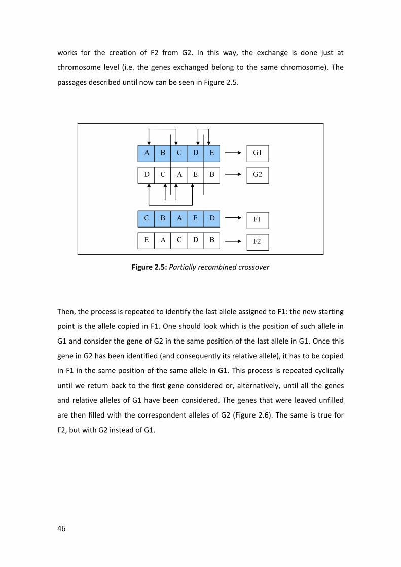
Another kind of crossover method is the so called “partially recombined crossover”.
The process starts again from two randomly selected G1 and G2 and two crossover
points. Considering the genes in between the two crossover points in G1 and looking
at the corresponding genes in between the two crossover points in G2, we can say
that, ideally, some couples are created (one for each gene in between the crossover
points). Specifically, in G1 (G2) it is possible to find the same alleles that are also in G2
(G1), even if in different positions, recreating therefore the couples defined through
the comparison between G1 and G2. The next step is the exchange of the alleles of
one couple of genes in G1, generating in this way the chromosome-child F1. The same
46
works for the creation of F2 from G2. In this way, the exchange is done just at
chromosome level (i.e. the genes exchanged belong to the same chromosome). The
passages described until now can be seen in Figure 2.5.
Figure 2.5: Partially recombined crossover
Then, the process is repeated to identify the last allele assigned to F1: the new starting
point is the allele copied in F1. One should look which is the position of such allele in
G1 and consider the gene of G2 in the same position of the last allele in G1. Once this
gene in G2 has been identified (and consequently its relative allele), it has to be copied
in F1 in the same position of the same allele in G1. This process is repeated cyclically
until we return back to the first gene considered or, alternatively, until all the genes
and relative alleles of G1 have been considered. The genes that were leaved unfilled
are then filled with the correspondent alleles of G2 (Figure 2.6). The same is true for
F2, but with G2 instead of G1.
47
Figure 2.6: Cyclical crossover
A drawback of the crossover operator is that allows to exclusively recombine genes
which are already in the population of the potential solutions and, therefore, it is not
possible to explore the space of the solutions in depth30. To accomplish such task, the
mutation operator is applied.
2.4.3 Mutation
The aim of this operation is to perturb the individuals-solution of the new population.
Literally, new alleles, which are not present in the initial chromosome-population, are
introduced in the population. Mutation allows to explore new sub-intervals of
solutions on which will then be performed a research in depth through the crossover
operator. Looking at the mutation operator from this perspective, we can say that it is
a “secondary” operator and Holland itself indeed wrote <<Mutation is a “background”
operator, assuring that the crossover operator has a full range of alleles so that the
30 Exploring the space of the solutions in depth implies limiting the risk that the Genetic Algorithm got stuck in regions of local optimum. The GA with only the crossover operator faces the risk of providing solutions with low explanatory power, since they would come from a limited sub-interval of solutions.
48
adaptive plan is not trapped on local optima […]. The mutation serves some
enumerative function, producing alleles not previously tried31>>.
As for the crossover operation, a certain probability 𝑝𝑚 is defined. Such probability
represents the probability that each allele of the chromosome taken into consideration
will change its value. Anyway, 𝑝𝑚 is lower than 𝑝𝑐.
There are different forms of mutation, depending on whether the representation is
binary or non-binary. For binary representations, mutation is from 0 to 1 or vice versa.
Instead, for non-binary representations, mutation is much more complex but usually
the recommended way of proceeding is to add a zero mean Gaussian number to the
original values.
There is no guarantee that this operation will provide better results, but at least we
are sure that, changing some part of the chromosomes, something new is created.
According to Gen and Cheng32 this operator helps in exploring new regions of the
multi-dimensional solution space.
Anyhow, besides the traditional reproductive-inspired operators of Selection,
Crossover and Mutation, there exist other less conventional operators such as
Inversion (discussed by Holland) and the Lamarckian operator (proposed by Gen and
Cheng).
2.5 Substitution phase
After the evaluation phase and the application of the different operators, with the final
objective of obtaining a new and better population, there exist mainly three methods
31 See: HOLLAND, J.H. (1992). Adaption in natural and artificial systems: an introductory analysis with applications to biology, control, and artificial intelligence. Page 111. MIT Press. 32 See: GEN, M., CHENG, R. (1997). Genetic Algorithm and Engineering Design. John Wiley & Sons, Inc. New York.
49
of substitution of the population from which the chromosome-parents were selected
with the one of the chromosome-children:
1. The “delete-all” substitution provides that the new population is constituted
merely by the chromosome-children and all the chromosome-parents are
completely deleted;
2. The “steady-state” substitution provides that the new population is constituted
both by the chromosome-parents and the chromosome-children. One
parameter needs to be set to define the proportion between parents and
children into the new population (i.e. how many parents need to be removed).
The criterion to choose which of them should be removed is based again on the
fitness score;
3. The “steady-state without duplicates” substitution is an amended version of
the “steady-state” substitution. The unique difference is that the duplicates of
chromosomes are deleted.
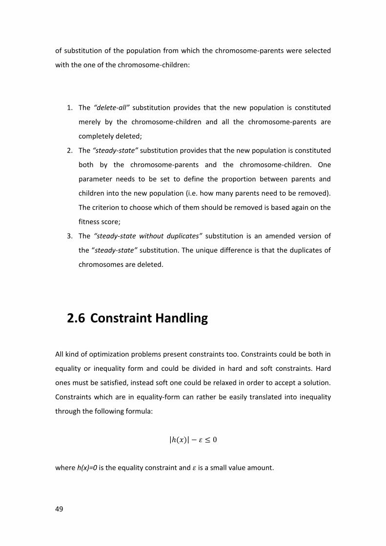
2.6 Constraint Handling
All kind of optimization problems present constraints too. Constraints could be both in
equality or inequality form and could be divided in hard and soft constraints. Hard
ones must be satisfied, instead soft one could be relaxed in order to accept a solution.
Constraints which are in equality-form can rather be easily translated into inequality
through the following formula:
|ℎ(𝑥)| − 휀 ≤ 0
where h(x)=0 is the equality constraint and 휀 is a small value amount.
50
In literature there exist different constraint handling methods when using
metaheuristics, which are usually classified in five different types:
➢ Methods based on preserving the feasibility of solutions;
➢ Methods based on penalty functions;
➢ Methods biasing feasible over infeasible solutions;
➢ Methods based on decoders;
➢ Hybrid methods.
For the aim of this thesis’ optimization problem, the suitable method could be the
penalty function method, which practically transform a constrained optimization
problem into an unconstrained one through the use of an additive penalty term or of a
penalty multiplier. Furthermore, these penalty methods can be grouped into seven
categories:
➢ Death Penalty;
➢ Static Penalties;
➢ Dynamic Penalties;
➢ Annealing Penalties;
➢ Adaptive Penalties;
➢ Segregated GA.
Again for this thesis purpose, the most suitable choice with regards to the different
penalties is the static penalties approach because the penalty parameters do not
change within generations and because they are applied to infeasible solutions only.
There are different ways to approach this method and here we present one of the
most known. It was initially presented by Morales A. K.33 in 1997, and it is based on the
penalization of the fitness function of infeasible solutions by using the information on
the number of violated constraints.
33 MORALES, A. K., QUEZADA, C. V., BATIZ, J. D., LINDAVISTA, C. (1997). A Universal Eclectic Genetic Constrained Optimization Algorithm for Constrained Optimization. Optimization, pages 2-6.
51
𝐹(𝑥) = {
𝑓(𝑥), 𝑖𝑓 𝑥 𝑖𝑠 𝑓𝑒𝑎𝑠𝑖𝑏𝑙𝑒,
𝐾 −∑ [𝐾
𝑚]
𝑠
𝑖=1, 𝑜𝑡ℎ𝑒𝑟𝑤𝑖𝑠𝑒.
where:
s is the number of non-violated constraints;
m is the total number of constraints;
K is a large pre-defined positive constant.
The value of K is generally chosen (by Morales et al.) equal to 1𝑥109 . The aim of this
large enough pre-defined penalty factor is to ensure the assignment of larger fitness
values to infeasible solutions compared to feasible solutions.
52
CHAPTER 3
Case Study: IAG – WACC computation
In this chapter the International Consolidated Airlines Group, S.A.
(IAG) company is introduced as the company chosen for the specific
case-study. There are both the industry and the company overview.
Then, there are the calculations of the different components of the
Cost of Capital, which will be used as model’s inputs for the
implementation of the Genetic Algorithm in the next chapter.
3.1 The Airline Industry Landscape
The company operates primarily in the Aviation, or Air Transport, industry, which
includes both passenger and cargo transportations.
This sector of the market consists of over 2000 airlines, providing services to nearly
3700 airports around the world and operating more than 23000 aircrafts on a daily
basis. In the last few decades, international airlines established different kinds of
alliances in order to expand and reach a global presence. Air Transport industry, as
well as airlines’ profitability, is highly correlated to economic, political and social
factors and, consequently, it is considered one of the most volatile industries. It is an
increasingly competitive and fast paced environment. Therefore, in order to
strengthen their very low profit margins34 and to keep such challenges under control,
airlines need constant improvements. Even though the overall profitability of the
world airlines lost 14.3% in 2018, analysts from S&P Global Ratings are broadly
optimist regarding the growth prospects of the airline industry, mainly thanks to the
34 The main reason is due to the extremely fast-growing low-cost carriers (LCCs), which fosters competition primarily in the pricing polices (hence lowering the profit margin).
53
rising desire of the young generation to travel more and more around the globe,
together with higher levels of spending on travelling costs among the older generation.
The major market drivers are the growing demand for air travel, the accessibility to air
travel thanks to low-cost carriers, the burgeoning e-commerce, the opening of new
routes and the opportunities offered by the incorporation of new technologies35. The
challenges, instead, are represented mainly by increasing fuel prices, labour expenses
and of course political uncertainties.
The European Union is currently home of 135 airlines, while America doesn’t count
more than 59 companies (American Airlines Group is the biggest one by revenues, fleet
size and passengers carried, while Delta Airlines is the largest airline by assets value
and market capitalization). Focusing on Europe, instead, the top 5 Airlines or Airline
Groups by passengers carried are: Lufthansa Group, Ryanair, International Airlines
Group (IAG), Air France – KLM, and easyJet.36
3.2 Company Overview
The International Consolidated Airlines Group (IAG) is an Anglo-Spanish registered
airline company in Madrid (Spain) with its operational headquarters based in London
(United Kingdom), whose shares are traded on the London Stock Exchange and
Spanish Stock Exchanges. It is one of the world’s largest airline groups with almost 600
aircraft flying to more than 250 destinations, carrying around 113 million passengers
each year. IAG's CEO is Willie Walsh.
35 The use of Biometrics and RFID for self-check-in, passport control, baggage tracking and security. In addition, airlines and airports are planning to use Artificial Intelligence (AI) and Blockchains according to SITA (Société Internationale de Télécommunications Aéronautiques - the world’s leading specialist in air transport communications and information technology). 36 Source: World Air Transport Statistics (WATS 2018), IATA – International Air Transport Association.
54
3.2.1 History
IAG is an Anglo-Spanish company registered in Madrid and was incorporated on April
8, 2010. The launch of the International Consolidated Airlines Group S.A. (hereinafter
“International Airlines Group” or “IAG”) company dates back to January 2011 after the
merger between British Airways and Iberia, the leading airline companies of United
Kingdom and Spain, respectively. Also, British Airways World Cargo and Iberia Cargo
merged, forming IAG Cargo. In December of the same year IAG made a deal with
Lufthansa, as cleared by the European competition authorities, for the acquisition of
British Midland International (BMI), whose fleet and routes were integrated with those
of British Airlines. IAG acquired BMI effectively in 2012. In addition, in 2013 IAG bought
Vueling, a leading Spanish short-haul airline. After the rejection of two offers, in 2015
IAG managed to acquire also the Irish airline Aer Lingus.
Furthermore, in response to increased competition in the low-cost long-haul market,
in the late 2017 a new subsidiary company, called LEVEL, was created.
Hence, IAG has become the parent company of British Airlines, Iberia, Vueling, Aer
Lingus and LEVEL.
3.2.2 Business Model
IAG’s vision is to be the world’s leading airline group and to maximize the creation of
sustainable value for both shareholders and customers.
Although the Group portfolio consists of distinct operating companies (from full
service long-haul to low-cost short-haul carriers, each targeting specific customer
needs and geographies), IAG relies on a common integrated platform which allows the
Group to exploit revenue and cost synergies (this would not be achievable in the case
of operating companies working alone), while maintaining simultaneously simplicity,
efficiency and their unique identities. This pursuit of gradually increasing value and
sustainable growth allows the Group to reduce costs and improve efficiency. IAG takes
advantage of these synergies opportunities by leveraging its scale, by engaging itself
55
with new innovation strategies and by increasing external B2B services. All these
strategies enhance productivity and create value for the customers. Figure 3.1 below is
a graphical representation of its business model.
Figure 3.1: IAG Company’s Business Model
Source: IAG Company’s website – Business Model & Strategy section
Furthermore, British Airways and Iberia are members of Oneworld alliance, which
brings together 13 of the world’s leading airlines and around 30 affiliates, allowing a
cooperative approach in different fields (such as scheduling and pricing) and
combining destinations spread all over the world. Some examples are the alliance
between British Airways, Iberia and American Airlines that connects Europe with the
United States of America, Canada and Mexico, or the one between British Airways,
Finnair, Iberia and Japan Airlines that connects Europe to Asia and Japan, or the one
between British Airways and Qatar Airways that connects the UK with Doha. This
alliance produces operating efficiencies and improves customer convenience and
choice, also allowing mixing and matching flights to get the best deals.
56
3.2.3 Profitability, financial and structure ratios
In a glance, looking at the profitability and main financial ratios of IAG (in Table 3.1), it
is possible to observe that the company had a great improvement in the efficiency of
the management and in terms of profitability moving from year to year. Nevertheless,
the situation changes focusing just on the ratios between 2016 and 2017, where the
company appears to make worse its efficiency and also profitability indicators become
lower. However, this was a really slight worsening and after that the company started
In detail, the ROE (Return On Equity) of the company had a huge increase during the
last year, which means that it had a great improvement in terms of profitability,
productivity and management efficiency. Also the ROA (Return On Assets), which
shows the percentage of how profitable the company’s assets are in generating
revenue, followed the same path of the ROE. The behavior of both the ratios could be
seen in Graph 3.1.
57
Graph 3.1: ROE & ROA ratios over last 5 years
For the other financial ratios considered, the situation is the same: the EBITDA and
EBIT margin variations suggest that the company improved its capacity to generate
value through the operational management (with the only already mentioned
exception between 2016 and 2017).
In Graph 3.2, the bottom line of the Consolidated Income Statement is the Net Income,
which reflects the total amount of revenue left over after all expenses and additional
income streams are accounted for, including also interests from debts and taxes.
Dividing it by the revenues and multiplying by 100, we obtain the Net Profit Margin,
which reflects a company’s overall ability to turn income into profit.
Here again the behavior is in line with the other financial ratios, as we can see from
Graph 3.2.
26,44% 27,39%
34,46%
28,98%
43,11%
4,24% 5,37%7,13% 7,38%
10,33%
0,00%
10,00%
20,00%
30,00%
40,00%
50,00%
2014 2015 2016 2017 2018
ROE ROA
58
Graph 3.2: IAG’s financial ratios over last 5 years
Finally, looking at the structure ratios, we can notice that the Current ratio, which is
the ratio between current assets and current liabilities and measures whether a firm
has enough resources to pay its debt over the next 12 months, slightly decreased
during the last year compared to the previous two but it is still around a value of 1.
Usually it is considered to be positive when its value is greater than 1. Anyway, this is
counterbalanced by the Leverage ratio (=Total Assets/Equity), which shows a really
good value (usually a good value is considered to be between 1 and 3). Another ratio
that gives useful information is the ratio between total liabilities and total assets. Since
it is a leverage ratio, the higher it is, the higher the risk is as well. For IAG Company the
value of this ratio is small enough to guarantee a good stability. The path of these
three ratios during the last 5 years can be seen in Graph 3.3.
10,64%
15,86%16,71%
15,06%
20,21%
5,10%
10,14%11,01%
9,89%
15,07%
4,97%
6,63%
8,65% 8,78%
11,87%
0,00%
5,00%
10,00%
15,00%
20,00%
25,00%
2014 2015 2016 2017 2018
EBITDA margin (%) EBIT (operating) margin (%)
Net Profit Margin (%)
59
Graph 3.3: IAG’s structure ratios over last 5 years
3.3 IAG’s Weighted Average Cost of Capital
From now on, the chapter will focus on the derivation of the Weighted Average Cost of
Capital. The costs of individual financing sources, precisely the Cost of Debt and the
Cost of Equity, have to be both estimated (since they are the only components of the
firm’s total capital) and weighted. To recap, the general formula of the Weighted
Average Cost of Capital (i.e., WACC) is:
𝑊𝐴𝐶𝐶 = 𝐾𝐸 ∗ [𝐸
𝐷 + 𝐸 + 𝑃𝑆] + 𝐾𝐷 ∗ [
𝐷
𝐷 + 𝐸 + 𝑃𝑆] + 𝐾𝑃𝑆 ∗ [
𝑃𝑆
𝐷 + 𝐸 + 𝑃𝑆].
In chapter two we defined the hybrid securities and, therefore, it is important to say
that since Convertible Bonds were already included in the consolidated financial
statement of the company under the voice of “Long-term borrowings – Bank and other
loans” and since the amount of Preferred Stock is equal to zero in 2018, for the
following analysis just Debt and Equity will be considered as the components of the
0,00 1,00 2,00 3,00 4,00 5,00 6,00 7,00
2014
2015
2016
2017
2018
Structure Ratios
Tot. Liabilities/Tot. Assets Leverage Current ratio
60
firm’s Capital. Considering such adjustment, the formula of the WACC can be simplified
in the following way:
𝑊𝐴𝐶𝐶 = 𝐾𝐸 ∗ [𝐸
𝐷 + 𝐸] + 𝐾𝐷 ∗ [
𝐷
𝐷 + 𝐸]
IAG operates in different countries and so it has to cope with different currencies.
However, the analysis is completely led in euros since all foreign operations are
translated into euros at the rate of exchange ruling at the balance sheet date. In other
words, all profits and losses coming from its operations are translated in euros at
average rates of exchange during the year.
3.3.1 Cost of Debt
Regarding the Cost of Debt, the first step is looking at the rating of the company. In
November 2018, S&P and Moody’s assigned IAG with a long-term investment grade
credit rating with stable outlook (BBB). From Table 1.2 of chapter one it is possible to
retrieve the default spread corresponding to the company’s rating (1.27%), to which
the risk-free rate is added in order to arrive at the real cost of debt. Since the firm is
settled in Spain, but operates in many different countries, in order to have a proxy of a
risk-free rate of the Euro-zone, the choice has been to take the mean of the 10-years-
maturity Treasury Bonds of the countries which IAG considers for taxation purposes
(precisely: UK, Spain and Ireland). This choice brings to a yield of 0.40%.
Hence, adding this risk-free rate to the firm’s specific default rate we get a pre-tax Cost
of Debt equal to 1.67%.
Since the vast majority of the Group’s activities are taxed in the countries of effective
management of the main operations (UK, Spain and Ireland with corporation tax rates
during 2018 of 19%, 25% and 12.5% respectively), the marginal tax rate chosen for the
61
analysis is the one reported by IAG itself as “The Group’s effective tax rate for the year”
and it is equal to 16.9%.
The after-tax Cost of Debt can be formalized as follows:
𝐾𝐷 𝑎𝑓𝑡𝑒𝑟 𝑡𝑎𝑥 = (1 − 𝑡𝑎𝑥 𝑟𝑎𝑡𝑒) ∗ 𝐾𝐷 .
Considering 16.9% as the final marginal tax rate for the entire Group and applying it to
the formula above, we get to an after-tax Cost of Debt of 1.39%.
3.3.2 Cost of Equity
The Cost of Equity, computed through the usual CAPM formula, depends on three key
components: the risk-free rate, the equity risk premium (ERP) for the firm and its
levered beta.
While all that does concern the risk-free rate has already been explained, some
attention on the other two components is needed.
In order to calculate the proper ERP, firstly, the chosen approach is the long-term
average historical approach because in this thesis we assume that the belief that
investors are rational is erroneous and because the purpose of the analysis regards
corporate finance (and the average historical is the best recognized approach in this
field). Secondly, the partitioning of revenues per country has been taken from the
consolidated financial statement of the company. Lastly, the risk of the business has
been considered as a weighted average of the risks of the countries in which IAG
Company operates (weighting the various countries’ equity risk premium by
considering the contribution of each geographical subdivision to the revenues).
62
Country Rating
(S&P 500)
Default
Spread ERP Revenues
% on the
Total
UK AA 0.56% 5.85% € 7 982.00 32.71%
SPAIN A 1.80% 7.09% € 4 064.00 16.65%
USA AA+ 0.00% 5.29% € 4 093.00 16.77%
Rest of the World
(mainly Asia
Pacific, Latin
America &
Caribbean, Africa
& Middle East)
4.06% 9.35% € 8 267.00 33.87%
Table 3.2: IAG – Revenue Subdivisions
For USA the final ERP is equal to the implied equity risk premium37 of 5.29% (exploited
by A. Damodaran’s tables – NYU Stern University website, updated in December 2018),
without therefore adding any default spread since it is considered as major developed
country. Instead, for the other countries, sovereign default spreads are usually used as
measures of additional country risk premiums that equity-analysts would demand for
investing in the equity of those countries. Hence, for UK and Spain, a small default
spread (based on the sovereign rating) is added to the implied equity risk premium,
giving a final ERP of 5.85% for UK and one of 7.09% for Spain. For the Rest of the World
the default spread has been computed as the median value of the various default
spreads of the countries belonging to Asia Pacific, Latin America & Caribbean, Africa &
Middle East (which are the countries, indicated by the firm itself, from where the other
revenues come), bringing to a final estimate of the ERP equal to 9.35%. Weighting then
these ERPs by the shares of revenues coming from the specific countries, the resulting
weighted average equity risk premium for IAG Company is 7.15%.
37 The implied equity risk premium is an alternative way to estimate risk premium. It does not require historical data or adjustments for country-specific risks. It is obtained from the difference between the present value of dividends growing at a constant rate and the risk-free rate. It will be our starting point.
63
Table 3.3 below incorporates the data of the selected countries belonging to the areas
where the other revenues come from (specifically, Asia Pacific, Latin America &
Caribbean, Africa and Middle East).
Country Region Moody's
rating
Rating-based Default Spread
Country Risk
Premium
Abu Dhabi Middle East Aa2 0.56% 0.69%
Angola Africa B3 7.34% 9.03%
Argentina
Central and South
America B2 6.21% 7.64%
Aruba Caribbean Baa1 1.80% 2.22%
Bahamas Caribbean Baa3 2.48% 3.06%
Bahrain Middle East B2 6.21% 7.64%
Bangladesh Asia Ba3 4.06% 5.00%
Barbados Caribbean Caa3 11.28% 13.87%
Belize
Central and South
America B3 7.34% 9.03%
Benin Africa B1 5.08% 6.25%
Bermuda Caribbean A2 0.96% 1.18%
Bolivia
Central and South
America Ba3 4.06% 5.00%
Botswana Africa A2 0.96% 1.18%
Brazil
Central and South
America Ba2 3.39% 4.17%
Burkina Faso Africa B2 6.21% 7.64%
Cambodia Asia B2 6.21% 7.64%
Cameroon Africa B2 6.21% 7.64%
Cape Verde Africa B2 6.21% 7.64%
Cayman
Islands Caribbean Aa3 0.68% 0.84%
Chile
Central and South
America A1 0.79% 0.98%
China Asia A1 0.79% 0.98%
Colombia
Central and South
America Baa2 2.15% 2.64%
64
Congo
(Democratic
Republic of) Africa B3 7.34% 9.03%
Congo
(Republic of) Africa Caa2 10.16% 12.50%
Costa Rica
Central and South
America B1 5.08% 6.25%
Côte d'Ivoire Africa Ba3 4.06% 5.00%
Cuba Caribbean Caa2 10.16% 12.50%
Curacao Caribbean A3 1.35% 1.67%
Dominican
Republic Caribbean Ba3 4.06% 5.00%
Ecuador
Central and South
America B3 7.34% 9.03%
Egypt Africa B3 7.34% 9.03%
El Salvador
Central and South
America Caa1 8.46% 10.41%
Ethiopia Africa B1 5.08% 6.25%
Fiji Asia Ba3 4.06% 5.00%
Gabon Africa Caa1 8.46% 10.41%
Ghana Africa B3 7.34% 9.03%
Guatemala
Central and South
America Ba1 2.82% 3.47%
Honduras
Central and South
America B1 5.08% 6.25%
Hong Kong Asia Aa2 0.56% 0.69%
India Asia Baa2 2.15% 2.64%
Indonesia Asia Baa2 2.15% 2.64%
Iraq Middle East Caa1 8.46% 10.41%
Israel Middle East A1 0.79% 0.98%
Jamaica Caribbean B3 7.34% 9.03%
Japan Asia A1 0.79% 0.98%
Jordan Middle East B1 5.08% 6.25%
Kenya Africa B2 6.21% 7.64%
Korea Asia Aa2 0.56% 0.69%
Kuwait Middle East Aa2 0.56% 0.69%
Lebanon Middle East B3 7.34% 9.03%
Macao Asia Aa3 0.68% 0.84%
Malaysia Asia A3 1.35% 1.67%
Maldives Asia B2 6.21% 7.64%
65
Mauritius Asia Baa1 1.80% 2.22%
Mexico
Central and South
America A3 1.35% 1.67%
Mongolia Asia B3 7.34% 9.03%
Montserrat Caribbean Baa3 2.48% 3.06%
Morocco Africa Ba1 2.82% 3.47%
Mozambique Africa Caa3 11.28% 13.87%
Namibia Africa Ba1 2.82% 3.47%
Nicaragua
Central and South
America B2 6.21% 7.64%
Nigeria Africa B2 6.21% 7.64%
Oman Middle East Baa3 2.48% 3.06%
Pakistan Asia B3 7.34% 9.03%
Panama
Central and South
America Baa2 2.15% 2.64%
Papua New
Guinea Asia B2 6.21% 7.64%
Paraguay
Central and South
America Ba1 2.82% 3.47%
Peru
Central and South
America A3 1.35% 1.67%
Philippines Asia Baa2 2.15% 2.64%
Qatar Middle East Aa3 0.68% 0.84%
Ras Al
Khaimah
(Emirate of) Middle East A2 0.96% 1.18%
Rwanda Africa B2 6.21% 7.64%
Saudi Arabia Middle East A1 0.79% 0.98%
Senegal Africa Ba3 4.06% 5.00%
Sharjah Middle East A3 1.35% 1.67%
Singapore Asia Aaa 0.00% 0.00%
Solomon
Islands Asia B3 7.34% 9.03%
South Africa Africa Baa3 2.48% 3.06%
Sri Lanka Asia B1 5.08% 6.25%
St. Maarten Caribbean Baa2 2.15% 2.64%
St. Vincent &
the
Grenadines Caribbean B3 7.34% 9.03%
Suriname Central and South B2 6.21% 7.64%
66
America
Swaziland Africa B2 6.21% 7.64%
Taiwan Asia Aa3 0.68% 0.84%
Tanzania Africa B1 5.08% 6.25%
Thailand Asia Baa1 1.80% 2.22%
Trinidad and
Tobago Caribbean Ba1 2.82% 3.47%
Tunisia Africa B2 6.21% 7.64%
Turks and
Caicos Islands Caribbean Baa1 1.80% 2.22%
Uganda Africa B2 6.21% 7.64%
United Arab
Emirates Middle East Aa2 0.56% 0.69%
Uruguay
Central and South
America Baa2 2.15% 2.64%
Venezuela
Central and South
America C 18.00% 22.14%
Vietnam Asia Ba3 4.06% 5.00%
Zambia Africa Caa1 8.46% 10.41%
Table 3.3: Asia Pacific, Latin America & Caribbean, Africa & Middle East Risk Premiums
Source: NYU Stern University – Datasets – Country Risk Premiums
Regarding the last component, we should introduce before the formula for the levered
beta (under the assumption that all of the firm’s risk is borne by the stockholders and
that debt creates a tax benefit to the firm):
𝛽𝐿 = 𝛽𝑈 ∗ [1 + (1 − 𝑡) ∗ (𝐷𝐸⁄ )] ,
where:
𝛽𝐿 is the levered beta for equity in the firm;
𝛽𝑈 is the unlevered beta of the firm (beta of the firm’s assets);
67
t is the marginal tax rate for the firm;
𝐷𝐸⁄ is the Debt/Equity ratio (market values).
The unlevered beta for a firm (also known as asset beta) depends on the types of
businesses in which it operates and its operating leverage. This industry unlevered
beta will be used later to re-lever the beta of the company, in order to have a more
precise estimate of its equity-risk component.
For this reason, the analysis starts by selecting 21 listed comparable firms (meaning
that they are mostly operating in the airlines industry). Table 3.4 below includes the
names of the selected comparable firms, together with the prevailing country in which
they operate (among these firms, 6 are European, 8 are American and 7 are Asian-
Pacific) and the corresponding marginal tax rate.
Comparable Firm Country (in which it
mainly operates) Marginal Tax Rate (KPMG)
RYANAIR Ireland 12,5%
AIRFRANCE KLM France 33,0%
LUFTHANSA GROUP Germany 30,0%
WIZZ AIR UK 19,0%
EASYJET UK 19,0%
FLYBE UK 19,0%
CATHAY PACIFIC Honk Hong 30,8%
JET AIRWAYS India 35,0%
THOMAS COOK India India 35,0%
MALAYSIA AIR Malaysia 24,0%
SINGAPORE AIRLINES Singapore 17,0%
THAI Thailand 20,0%
PEGASUS Turkey 22,0%
DELTA AIRLINES USA 27,0%
SKYWEST INC USA 27,0%
UNITED AIRLINES - UNITED CONTINENTAL HOLDINGS USA
27,0%
68
AMERICAN AIRLINES USA 27,0%
SOUTHWEST AIRLINES USA 27,0%
ALLEGIANT TRAVEL CO USA 27,0%
SPIRIT AIRLINES INC USA 27,0%
JETBLUE AIRWAYS CORP USA 27,0%
Table 3.4: List of IAG’s Comparable Firms
The unlevered beta for each company has been estimated according to the following
formula:
𝑙𝑒𝑣𝑒𝑟𝑒𝑑 𝑏𝑒𝑡𝑎
1 + (1 − 𝑚𝑎𝑟𝑔𝑖𝑛𝑎𝑙 𝑡𝑎𝑥 𝑟𝑎𝑡𝑒) ∗𝐷𝐸
.
The levered beta has been retrieved from Bloomberg (calculated against 5 years’
worth of weekly data of the relevant stock index), while the marginal tax rate is the
one of the countries each company belongs to and earns its operating income and it
has been retrieved from KPMG website38.
As stated in the second chapter, the analysis should be implemented with the use of
market values (rather than the book values) for Equity and Debt. The market value of
equity, which is usually the number of shares outstanding multiplied by the current
stock price, has also been taken from Bloomberg39.
Instead, as suggested by A. Damodaran, the estimation of the market value of debt
could be formalized through the following formula.
38 KPMG is a global network of professional firms providing Audit, Tax and Advisory services. To retrieve the table for corporate marginal tax rates visit: https://home.kpmg/xx/en/home/services/tax/tax-tools-and-resources/tax-rates-online/corporate-tax-rates-table.html 39 This choice comes from the fact that using average stock prices over time is not good practice since we want to measure the cost of raising funds today. Bloomberg, instead, considers multiple classes of shares to provide its computations.
42 FONSECA, C. M., FLEMING, P. J. (1993). Genetic algorithms for multi-objective optimization: Formulation, discussion and generalization. Proceedings of the 5th International Conference on Genetic Algorithms. Ubana-Champaign, I11. Pages 416-423.
77
The Multi Objective Genetic Algorithm tries to optimize the components of a vector-
valued objective function, which, in our case, consists of two different objectives (i.e.,
the minimization of the Weighted Average Cost of Capital and the maximization of the
Interest Coverage Ratio). Besides the setting of the objective functions, the optimal
solutions that we want to find are also subject to some specific constraints (i.e., limits
on the single financing components ratios) that have to be included in the
configuration of the algorithm in MATLAB software. The problem can be formalized as
In the above described problem, the voice “Subject to” sets the constraints to be
applied to this specific problem solver:
78
• 𝐷 + 𝐸 = 1 means that the sum of Debt and Equity constitutes 100% of the
firm’s Total Capital;
• 0.2 ≤ 𝐷 ≤ 0.8 fixes 20% minimum and 80% maximum levels on the debt ratio
in order to guarantee repayment capacity and take advantage of the tax-shield;
• 0.2 ≤ 𝐸 ≤ 0.8 fixes a 20% minimum base and an 80% maximum limit on the
equity ratio for the stability of the capital structure.
With regards to the ICR, the higher it is, the better it is, since it means more ease in the
payments of dividends and/or interests on debt. Nevertheless, this measure alone can
not be considered as an exhaustive indication of financial difficulty, and it should be
instead evaluated through a deeper dive into the firm’s financial statement (looking
for example at other liquidity and solvency ratios). The choice, however, fell on the ICR
because it represents the other side of the coin with respect to the WACC, in the sense
that a higher Debt ratio leads to a decrease in the WACC (positive consequence) but
also to a decrease in the ICR (negative consequence). Minimizing the first function and
maximizing the second, this thesis aims at finding a set of optimal solutions combining
these two conflicting objectives. When talking about conflicting objectives we refer to
the fact that the equity-shareholders’ target is not aligned with the one of the debt-
holders. Indeed, the equity-shareholders’ target is the pursuit of the company’s
economic interests, while debt-holders would like the company to keep a lower debt
ratio in order to be able to repay it. Hence, firms have incentives in the reduction of
the use of private equity for their operations in order to raise the rate of return. On
the contrary, an increase in the use of private equity for operations would
consequently lead to a decrease in the debt ratio, which would in turn lessen the
burden of debt service and improve the firms’ financing stability. The reduction in the
private equity’s utilization is instead carried out through an increase of the debt ratio,
which will consequently reduce the WACC too. However, firms should pay attention at
the impact of the financial leverage because, raising too much their debt, they risk to
reach a point where the debt level becomes unsustainable (because of the too high
interest rates). From such perspective, the Interest Coverage Ratio may be interpreted
as a threshold ratio defining an acceptable level for lenders, who want to evaluate the
79
amount of the loan that can be covered by the firm’s cash flow or other financial
resources. Indeed, companies that do not keep a proper level of debt ratio usually face
two consequences:
1. Costs of financial distress;
2. Bankruptcy costs.
The costs of financial distress can be attributed to the inability to negotiate long-term
supply-contracts in the future. Furthermore, at some point the additional value of the
interest tax shield would be offset by the increase in expected bankruptcy cost. At this
point the value of the firm will start to decrease as more debt is added and the most
direct drawback will be the disincentive to debt financing.
In our specific IAG Company’s case study, the EBIT can be found in the Income
Statement of the company, retrieved in the section “Investors and shareholders –
Results and reports” of their website, under the name of Operating profit
(𝑂𝑝𝑒𝑟𝑎𝑡𝑖𝑛𝑔 𝑃𝑟𝑜𝑓𝑖𝑡 = 𝑇𝑜𝑡𝑎𝑙 𝑅𝑒𝑣𝑒𝑛𝑢𝑒 − 𝑇𝑜𝑡𝑎𝑙 𝑒𝑥𝑝𝑒𝑛𝑑𝑖𝑡𝑢𝑟𝑒 𝑜𝑛 𝑜𝑝𝑒𝑟𝑎𝑡𝑖𝑜𝑛𝑠) and it
is equal to 3,678 million euros, while the Interest Expense can be found under the
name of finance costs, again in the Income Statement. Such finance costs are mainly
interest expenses on bank borrowings, financial leases or other borrowings. Since all
these voices (i.e., interest expenses, financial leases) fall into the definition of debt and
could be directly related to it, the income statement finance costs-voice could be
described and represented as a function of debt. The approximation of this function
has been computed in Excel taking into consideration debt and finance costs values of
the last five years for IAG Company. A linear approximation results in the following
function:
𝑦 = 0.0509𝑥 − 150.15,
where x represents the book value of debt.
80
Clearly, as debt increases, interest expenses increase as well. The parameter in front of
x (i.e., debt value) is small because the amount of debt is expressed in million euros
while the value of the interest expenses (i.e., finance costs) is in thousands.
The plot of the finance costs approximation as a function of debt can be seen in Figure
4.3 below, where also its R-squared value (𝑅2 = 0.9869) is reported.
Figure 4.3: Finance costs estimation as a function of Debt
The scope of this thesis is the specification, through a Multi-objective Genetic
Algorithm, of an optimized capital structure model in order to reach a balanced
structure between the interests of the company itself and its creditors. This balanced
structure synchronizes both profitability through the minimization of WACC (in the
meaning of average rate of return the company expects to compensate to all its
different investors) and repayment capacity through the maximization of the Interest
Coverage Ratio, where the numerator (i.e., the EBIT) is implicitly assumed constant for
the next calculations while the denominator (i.e., the Interest expense) is represented
81
by the linear approximated function (depending on the Debt ratio). The reason behind
this balanced structure is that any company needs to find an optimal point where its
profitability is maximized considering also the lenders’ perspective.
4.3 Model Specifics
In order to implement our specific Multi-objective Genetic Algorithm, the last updated
version of the software MATLAB has been used, precisely version MATLAB R2019b. In
this version there are different graphic user interfaces called toolboxes. To program a
MOGA, one can use the gamultiobj-solver in the OPTIMIZATION-toolbox. Since the
basic calculation of the MOGA in the OPTIMIZATION-toolbox in MATLAB is fitted to
minimum-optimization, for the maximum-optimization of our second objective
function (the ICR depending on the debt ratio) we need to multiply it by -1. The
gamultiobj-solver, through a set of operators that work on the initial randomly
generated population, computes the next generation of the population using the non-
dominated rank43 and a distance measure44 of the individuals. Furthermore, this solver
uses a controlled elitist45 genetic algorithm. An elitist genetic algorithm favors the
genes (i.e., the individuals) with better fitness value (i.e., lower rank). A controlled
elitist genetic algorithm also favors individuals which can help in the population
diversity’s increase (even if they have lower fitness value). Maintaining the diversity in
the population is important for the convergence to the optimal set of solutions on the
Pareto front.
43 The non-dominated rank is assigned to each individual using the relative fitness. Individual p dominates q (i.e., p has lower rank than q) if p is strictly better than q in at least one objective and p is no worse than q in all objectives. Individuals p and q are considered to have equal ranks if neither dominates the other. 44 The distance measure of the individuals is used to compare individuals with equal rank. It is a measure of how far an individual is from the other individuals with the same rank. 45 The concept of “elitism” is generally related to memory (in the sense of remember the best solution found). Particularly, for evolutionary algorithms like MOGA, elitism involves copying a small portion of the best solutions found into the next generation. The use of unchanged fittest candidates for building the next generation ensures that the algorithm does not waste time re-discovering previously discarded solutions.
82
Instead of using the OPTIMIZATION-toolbox and the gamultiobj-solver, one can write
the code for the MOGA implementation. In a separated MATLAB file there are the two
objective functions’ formulation and the imputation of the number of variables, which
in our case is just one (i.e., the debt ratio) since the other unknown component of the
total capital (i.e., the equity ratio) can be retrieved simply by computing 1 − 𝑥, where
x is our decision variable. The structure of the code is set in the way shown in Figure
Given these parameters, the algorithm starts from a population of 100 random
solutions of our decision variable x (i.e., the debt ratio). The population type is then
used to specify the input type for the fitness function. The default type is
doubleVector, which represents the option used for mixed integer programming. The
algorithm continues its process until it reaches one of the possible stopping criteria
(that will be examined later on in this chapter). In our specific case we will see that the
algorithm stopped because it exceeded the maximum number of generations (i.e.,
iterations).
The Selection method adopted for selecting the parents for the next generation is the
Tournament-Selection with default size-value because it is the only available method
for the gamultiobj-solver in MATLAB. The Tournament-Selection picks each parent by
46 DEB, K., AGRAWAL, S., PRATAP, A., MEYARIVAN, T. (2000). A fast elitist non-dominated sorting genetic algorithm for multi-objective optimization: NSGA-II. Springer, Berlin.
84
randomly deciding tournament size players and then chooses the best individual out of
them to be a parent.
The designated function picked for Crossover, which combines two individuals (i.e., the
parents) to create a crossover child for the next generation, has been the Scattered
crossover with the default crossover-probability. The Scattered crossover creates a
random binary vector and selects the genes where the vector is equal to 1 from the
first parent and the genes where the vector is equal to 0 from the second parent,
combining then these genes to form the child. Most of the previous options (included
the Scattered crossover) can not be used in the case in which linear constraints are
present, because it may cause the population not to satisfy the constraints. Since we
do not have linear constraints, we set the reproduction, which specifies how the
Genetic Algorithm generates next generation’s children, through the CrossoverFraction
option. This option determines the fraction of the population at the next generation
that is created by the crossover function.
The other Genetic Algorithm’s operator is the mutation, which causes small random
changes in the genes of the population in order to create mutated children. The option
selected for our specific problem is the Adaptive feasible, which randomly generates
directions that are adaptive with respect to the last successful generation. Usually the
mutation probability is a constant value (i.e., all chromosomes have the same
likelihood of being subject to mutation, irrespective of their fitness). With this specific
option (i.e., keeping a step length along each direction), mutation becomes a function
of fitness. In this way bounds and constraints are satisfied, the chance of disrupting a
high-fitness chromosome is decreased and the exploratory role of low-fitness
chromosomes is best exploited.
In addition, in table 4.2 are reported also all the options under which our specific
MOGA-model has been programmed.
85
Multi-objective Options Value
Pareto Fraction 0.2
Distance Measure Function Phenotype
Function Tolerance 1e-4
Maximum Stall Generations 150
Table 4.2: Multi-objective options
The Pareto Fraction is a scalar from 0 to 1 which determines the fraction of the best fit
genes to keep on the first Pareto front in order to maintain a diverse population. While
its default value is 0.35 (i.e., the solver will try to limit the number of individuals in the
current population that are on the Pareto front to 35% of the population size), for our
specific optimization problem a 20% fraction has been decided in order to keep the
most fit solutions down to a reasonable number, maintaining anyway a diverse
population.
The Distance Measure Function is a measure of the concentration of the population
computed by comparing the distance between individuals with the same rank in the
function space (through the function handle phenotype). The distance function helps in
maintaining diversity on the Pareto front by favoring the genes that are relatively far
away on the front. These two options (Pareto Fraction and Distance Measure Function)
together control the elitism of the Genetic Algorithm.
The Function Tolerance is a measure that is used to determine when the algorithm has
to stop in the case in which the geometric average of the relative change in the spread
value47 of the Pareto solutions (i.e., the average relative change in the best fitness
function value) over Maximum Stall Generations48 option (default value is 100) is less
than Function Tolerance option and the spread value is smaller than the average
spread over the last Stall Generations option (in a simpler way we can say that the
algorithm stops if the spread is small). The 0.0001 value specified for the Function
47 The spread is a measure of the movement of the Pareto front. The coefficient for the geometric average of the spread-distance calculation is 0.5. 48 The value of Maximum Stall Generation is based on a test (i.e., StallTest) for a geometric weighted average relative change.
86
Tolerance is the default value for Multi-objective optimization problems using Genetic
Algorithms. The other potential conditions causing the stop of the solver are displayed
at the end of the process as an output argument under the voice of ExitFlag, which is
an integer. These additional stopping conditions could be the reach of the maximum
number of generations, the achievement of an output function, the failed attempt of
reaching a feasible point or the exceeding of the time limit.
4.4 Results
In the last line of the code reported in Figure 4.2 it is possible to see that in the square
brackets the user has to insert the output arguments. The first two output arguments
returned by gamultiobj are X (vector of the points of the decision variable on the
Pareto front) and FVAL (the objective functions’ values at the points’ values X). The
third and fourth output arguments (exitFlag and Output) return the reason why the
MOGA stopped and information about the performance of the gamultiobj solver (i.e.,
the type of problem, the total number of generations, the total number of function
evaluations, the average distance49, the spread, the maximum constraint violation at
the final Pareto set).
In the following table the X and FVAL values are reported. Each row of FVAL represents
the WACC and ICR function values (in this specific optimization problem) at one
Pareto-point in X (the set of the optimal selected debt ratios). In addition, there is also
the respective equity ratio for each x-point. All the values, except the equity ratio that
is simply computed by subtracting the x-value from 1, are the results of the
optimization problem computed by the gamultiobj solver in MATLAB.
49 The average distance is, by default, the standard deviation of the norm of the difference between Pareto front points and their mean.
87
The first line of table 4.4 has been added later and colored in light-blue in order to
show which are the actual (2018) values of IAG company.
Table 4.4: Decision Variable and Objective function values on the Pareto front
All the values of the ICR have to be read as positive values, since the negative sign is
simply because the gamultiobj solver automatically minimizes the objective functions
and so we had to multiply by -1 the ICR function to maximize it. It is possible to notice
that the minimum optimum x-value is a Debt ratio equal to 52,19%, so well above the
88
minimum set by the lower bound of 20%, while the maximum optimum is equal to
79,99% (the maximum set by the upper bound of 80%).
In figure 4.5 below is instead reported the pace of the debt ratio in each optimal
solution of the Pareto front produced.
Figure 4.5: Debt ratio values on the Pareto front
As we have already described in the previous paragraph, the algorithm stops at some
point when it meets one of the stopping criteria. The reason why our MOGA stopped
producing the results of the above figure and table is reported in the following figure.
Figure 4.6: End of MOGA optimization
89
The optimization process terminated because the algorithm reached the maximum
number of generations (i.e. 150), returning the x-values on the Pareto front with an
average distance between each other of approximately 0.011.
Through the PlotFcn option of the gamultiobj in MATLAB, the different data computed
by the algorithm can be plotted in different ways showing different features. I selected
the most interesting ones for this thesis’s purpose in the figure below.
Figure 4.7: gamultiobj plots
90
The different plots above show different features for each graph:
➢ The graph on the top left corner is the Pareto front for the two objective
functions;
➢ The graph on the top right corner shows the average distance between
individuals at each generation;
➢ The graph on the middle-left is called genealogy of the individuals. The lines are
colored between the generations, based on the operator that performed a
change on the chromosomes of one generation going toward the next one: red
lines represent mutated children, while blue lines represent crossover children;
➢ The graph on the middle-right shows an histogram of the initial population
individuals’ ranking. Individuals with rank equal to 1 are the ones on the Pareto
front (i.e., 20 solutions), the individuals with rank equal to 2 are lower than at
least one individual with rank equal to 1, therefore close to optimum but not
on the optimal Pareto frontier, and so on;
➢ The graph on the bottom left corner represents the average spread (i.e., the
measure of the movement of the Pareto frontier) as a function of the
generations’ number.
Adding the actual position of IAG Company (referring to the 2018 book values) with
respect to the optimal solutions found by the algorithm it is possible to understand
which are the changes that managers could make on the proportions of the company’s
capital components in order to reach the optimal capital structure analysed
(maximizing therefore the company’s profitability, while keeping an optimal level of
debt-repayment capacity). Such analysis can be performed looking at the graph 4.1
below, where the yellow point shows IAG’s actual capital structure.
91
Graph 4.1: IAG Company’s Pareto front with WACC minimization and
Interest_Coverage_Ratio as objective functions
On the x-axis and y-axis of the above graph there are the first and the second objective
functions: the WACC and the ICR, respectively. The blue, red and green points
constitute the Pareto optimal set (i.e., the Pareto front) found by running the Multi-
objective Genetic Algorithm. These optimal solutions are signed with three different
colors because I wanted to further skim the solutions. Even if, usually, in the economic
literature, an ICR of value of three (and above) is considered optimal, the additional
skimming is made clear through the red points, which denote the solutions found by
the algorithm for which the ICR is below 15 (that is the nearest rounded value to the
actual ratio of 15.42 for IAG Company). The reason behind such assignment of a
minimum floor for the ICR is that an higher ICR allows to take into consideration also
the involvement of different uncertainties in the financial environment. This skimming
is, however, performed just on the ICR since the value of the WACC changes less than
proportionally with respect to the ICR when there are changes in the debt value.
Indeed, the minimum and the maximum values of the WACC on the Pareto front are
92
3.15% and 5.65% respectively, while the minimum and maximum values for the ICR are
5.77 and 22.28.
The green point represents instead the closest point (in debt-change absolute terms)
to the actual position of IAG Company. IAG’s actual position in the above graph is
signed with the yellow color and shows the company’s debt level at the end of 2018.
Given the vector of solutions provided by the MOGA, the additional skimming on the
corresponding ICRs and considering the closest position from the actual one in debt-
change absolute terms, our suggestion is to move to this point (signed with the green
color) as soon as possible. At this proposed optimal setting, 47.87% of the total capital
should be funded by equity investment, and consequently the remaining part (52.13%)
would be financed with bank debt. Since actually (at the end of December 2018) debt
amounts to 7.5 billion, in order to reach the proposed optimal point (that is the second
to last row in Table 4.4) the managers of IAG Company should decrease debt by 0.64%.
A decrease of this kind may be carried out either by repaying part of its bank loans,
either by buying back some corporate bonds for a value of 48 million euros.
93
Conclusion
The proposed model is built to deal with the optimization of IAG Company’s capital
structure satisfying the two objectives of minimizing the WACC (i.e., Weighted Average
Cost of Capital) and maximizing the ICR (i.e., Interest Coverage Ratio).
Precisely, it should be noted that only the available book value data for the last year
have been considered (with the only exception for the estimation of finance costs as a
function of debt, for which five years book values have been utilized) and therefore
the analysis is centered only on the relative debt and equity weights.
In order to make an adequate evaluation (i.e., in the proper environment) and a
precise analysis, corporate analysts should consider first the firm’s life-cycle stage. The
usual companies’ life-cycle is shown in Figure 5.1.
Figure 5.1: Company’s Life Cycle
94
It is clear that, for example, at the Start-up or Early Stage (when the company is just at
the beginning of its business’ development), revenues could be negative (hence, the
company can not take advantage of the tax-shield triggered by the leverage effect) and
that the financing requirements are obviously high. Consequently, the debt ratio will
be high too. When the firm goes toward the end of its life-cycle (i.e., in the
Development or Replacement Stage through an hypothetical IPO – Initial Public
Offering), most likely, there would be enough money (coming from the Cash Flow and
from Private Equity) to cover the various activities and investments. This will in turn
produce a decrease in the debt ratio.
Secondly, corporate analysts should perform economic and qualitative analysis on the
company of interest and on the sector or business environment in which it operates,
before running the Genetic Algorithm to find the optimal solutions.
In addition, it is important to underline that, for optimizing a capital structure, the
objective functions must be chosen carefully because this is not a model ready to be
applied to any company or to address any business-environmental condition. Indeed,
setting for example two objectives that are not conflicting between each other
(depending on the decision variables chosen) one runs the risk of incurring in results
that are not really significant. For the sake of clarity, keeping the debt ratio as decision
variable and setting as objective functions the minimization of WACC and the
maximization of ROE (i.e., Return on Equity), the specific MOGA-model described in
this thesis produces just a singular result. In fact, running the algorithm with these two
objective functions, the Pareto front collapses in one single point (i.e., the sole optimal
solution). The output after the run of the MOGA with these two objective functions is
illustrated in Figure 5.2.
The reason behind the production of a solution solely derives from the fact that,
increasing the debt-ratio, the WACC-function declines while the ROE-function rises
(i.e., the two objective-function lines intersect). WACC declines because of the tax
shield-effect generated by debt, while ROE increases since the denominator of this
ratio decreases as the debt value rises, as demonstrated by its formula, that is
displayed below.
95
𝑅𝑂𝐸 =𝑁𝐼
𝐸
where NI and E represent Net Income and Equity, respectively.
In the IAG-specific case-study Equity is equal to 1 − 𝐷𝑒𝑏𝑡50.
Figure 5.2: gamultiobj plots with WACC-minimization and ROE-maximization as
objective functions
However, the model presented in this thesis bears some limitations. The most relevant
one is given by the fact that there are many assumptions. First, modifying the debt and
equity values (or, equivalently, their weights) also the other voices of the Income
Statement and of the Balance Sheet will change consequently. Second, it is not
50 This is true only in our specific case study because the capital of the company under analysis is actually composed only by Equity and Debt and there are not mixes of the two (i.e., hybrid securities).
96
reasonable to assume that the EBIT (i.e., the Operating Income) remains stable over
the years because it is subject both to movements of revenues and costs as its formula
demonstrates:
𝐸𝐵𝐼𝑇 = 𝑅𝑒𝑣𝑒𝑛𝑢𝑒𝑠 − 𝐶𝑜𝑠𝑡𝑠.
In addition, the ICR should be evaluated together with other ratios possibly indicating
financial difficulty (i.e., liquidity and/or solvency ratios) and should not be considered
alone as exact indicator of financial trouble.
Last but not least, the main limitation is the availability of data. This analysis has been
led using only the results and the data of the Company published on its website,
through which it is not possible to have real and exact function estimations. Indeed, in
order to have a more precise estimation, the knowledge of the different terms of loan
contracts stipulated with the banks which finance the firm could be helpful for the
calculation of the real interest expense. A greater availability of data may also bring to
an improvement of the finance costs’ (i.e., interest expenses) linear approximation by
adding further points, accomplished for example by considering a wider time-horizon.
Moreover, the fact that the firm operates in different countries (with different taxation
regimes and even different currencies) adds even more difficulties in the estimation of
the different functions.
Given the fact that here everything is assumed to remain stable and that there could
not be an exact prediction about the revenues a company could earn during the year
following, what can be tested in possible future researches is the combination of such
MOGA-model with some forecasting techniques (i.e., Monte Carlo simulations with
regards to the revenues or cash flows) in order to better estimate the potential
changes that companies might undertake.
Further improvements may be brought also by substituting the maximization of ICR
with some other objective functions making use of different kinds of ratios (the
alternatives could be represented by profitability ratios or turnover ratios) and setting
other solvency ratios or debt ratios as model’s constraints.
97
98
Bibliography
AFRASABI, J., AHMADINIA, H., HESAMI, E. (2012). A Comprehensive Review on
Capital Structure Theories. The Romanian Economic Journal. Vol XV(45), pages 3-
26.
BABUSIAUX, D., PIERRU, A. (2001). Capital Budgeting, Investment Project Valuation
and Financing Mix: Methodological Proposals. European Journal of Operational
Research. 135, pages 325-337.
BAKATJAN, S., ARIKAN, M., TIONG, R.L.K. (2003). Optimal capital structure model
for BOT power projects in Turkey. Journal of Construction Management and
Engineering. ASCE. 129(1), pages 89-97.
BAUER, R. J. Jr. (1994). Genetic Algorithms and Investment Strategies. Wiley.
BRANDIMARTE, P. (2001). Numerical methods in finance: A Matlab-based
instruction. Wiley and Sons, Inc., New York.
CHEN, B., MAO, C.K., HU, J.L. (2005). The optimal debt ratio of public-private
partnership projects. Journal of Construction Management. 15(3), pages 239-253.
COELLO, CARLOS A., L. G., B. V. (2007). Evolutionary Algorithms for Solving Multi-
Objective Problems. Genetic and Evolutionary Computation. Springer Science &
Business Media, LLC, second edition.
DAMODARAN, A. (2015). Applied Corporate Finance. Wiley, Fourth edition.
99
DEB, K. (1995). Real-coded Genetic Algorithms with Simulated Binary Crossover.
Studies on Multimodal and Multiobjective Problems. John Wiley & Sons, Inc. New
York. Writing, 9, pages 431-454.
DEB, K., AGRAWAL, S., PRATAP, A., MEYARIVAN, T. (2000). A fast elitist non-
dominated sorting genetic algorithm for multi-objective optimization: NSGA-II.
Springer, Berlin.
DEB, K. (2001). Multi-Objective Optimization Using Evolutionary Algorithms. John
Wiley & Sons Ltd. The Atrium, Southern Gate, Chichester, West Sussex PO19 8SQ,
England.
DIAS, A., IANNOU, P.G. (1995). Debt capacity and optimal capital structure for
privately financed infrastructure projects. Journal of Construction Management
and Engineering. ASCE. 121(4), pages 404-414.
ECB. (2005). The evolving framework for corporate governance. Monthly Bulletin. May
2005, pages 88-90.
FENG, K., XIONG, W., WU, C., XUE, Y. (2017). Optimizing an Equity Capital Structure
Model for Public-Private Partnership Projects Involved with Public Funds, Journal of
Construction Engineering and Management. 143(9).
FONSECA, C. M., FLEMING, P. J. (1993). Genetic algorithms for multi-objective
optimization: Formulation, discussion and generalization. Proceedings of the 5th
International Conference on Genetic Algorithms. Ubana-Champaign, I11. Pages
416-423.
GEN, M., CHENG, R. (1997). Genetic Algorithms and Engineering Design. John
Wiley & Sons Ltd. New York.
100
GOLDBERG, R., A. A., J. L. (2005). Evolutionary Multiobjective Optimization:
Theoretical Advances and Applications. Springer London Ltd, first edition.
HAUPT, R. L., HAUPT, S. E., WILEY, A. J. (2004). Algorithms: Practical Genetic
Algorithms. John Wiley & Sons, Inc. Hoboken, New Jersey.
HOLLAND, J.H. (1992). Adaption in natural and artificial systems: an introductory
analysis with applications to biology, control, and artificial intelligence. Page 111.
MIT Press.
IYER K. C., SAGHEER M. (2012). Optimization of bid-winning potential and capital
structure for build-operate-transfer road projects in India. Journal of Management
in Engineering. 28(2), pages 104–113.
KNOWLES, J. (2000). Approximating the non-dominated front using the Pareto