ùPresentation mode9Print this pageFavouriteFeedbackǃShare this page

TwitterFacebookLinkedInÈGoogle +ÓEmail

ÛSitemapĝTeaching materials

ù9ǃ

TwitterFacebookLinkedInÈGoogle +ÓEmail

Ûĝ

Trajectory of a balloonIntroduction

In this investigation the projectile motion of a balloon will be compared to the theoretical model bycalculating predicted range and maximum height from the equations of motion. The balloon isprojected by stretching it through a cardboard tube (toilet paper roll) and its trajectory measured byanalysing video. The aim of the experiment is to find out how close to the theoretical model this motionis and to attempt to explain any deviations.

The balloon launcher

To analyse the motion of a flying balloon it is important that it is projected with the same velocity eachtime. To launch the balloon it was stretched inside a cardboard tube and suddenly released asillustrated in fig.1.

We use cookies. By continuing to use this website you are giving consent to cookies being used. Readmore close

Fig.1 the balloon launcher

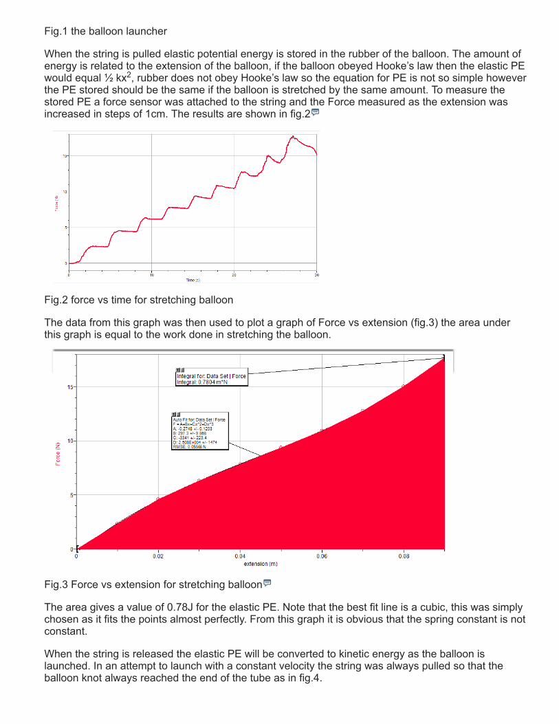
When the string is pulled elastic potential energy is stored in the rubber of the balloon. The amount ofenergy is related to the extension of the balloon, if the balloon obeyed Hooke’s law then the elastic PEwould equal ½ kx , rubber does not obey Hooke’s law so the equation for PE is not so simple howeverthe PE stored should be the same if the balloon is stretched by the same amount. To measure thestored PE a force sensor was attached to the string and the Force measured as the extension wasincreased in steps of 1cm. The results are shown in fig.2

Fig.2 force vs time for stretching balloon

The data from this graph was then used to plot a graph of Force vs extension (fig.3) the area underthis graph is equal to the work done in stretching the balloon.

Fig.3 Force vs extension for stretching balloon

The area gives a value of 0.78J for the elastic PE. Note that the best fit line is a cubic, this was simplychosen as it fits the points almost perfectly. From this graph it is obvious that the spring constant is notconstant.

When the string is released the elastic PE will be converted to kinetic energy as the balloon islaunched. In an attempt to launch with a constant velocity the string was always pulled so that theballoon knot always reached the end of the tube as in fig.4.

2

fig.4

To test if this always gave a constant velocity some preliminary experiments were performed launchingthe balloon horizontally off the end of the table. This was done by eye, watching where the balloonlanded each time and marking the position on the floor with a piece of chalk. The results are shown intable 1

Table 1

Due to the method of marking the ball after it had landed the uncertainty in the lengths was estimatedto be ±2cm. The range of values is from 117 – 175 cm so the initial velocity does not seem to beconstant. It was noticed that releasing the string cleanly was quite difficult, this might have caused thelarge range of velocities in an attempt to improve this a knot was tied in the end of the string. This knotseemed to be much easier to release cleanly so a second experiment was performed to see if therange was more consistent, the results of launching with a knot are shown in table 2.

Table 2

Now the range is from 155 – 180. The measurements were made in order; top row followed by bottomrow. It is apparent that the launching becomes more consistent with practice.

Measuring initial velocity

To measure the launch velocity the motion was recorded with a video camera and analysed withLoggerPro. First attempts were made with a computer webcam but the picture resolution was ratherpoor so a mobile phone was used instead. The camera was set up on a table next to the motion sothat the lens was roughly in the middle of the motion. This was done to reduce any parallax effects thatwould distort the lengths. To set the scale a 1 m ruler was held in the plane of the motion as in fig.5

Fig.5 setting the scale in LoggerPro.

Once the scale has been set the video analysis tools in LoggerPro were used to plot the trajectory ofthe balloon on the video. Even with the phone camera some of the images were a bit blurry, theballoon often appearing as 3 images. An example of how this was done is shown in fig.6.

Fig.6 marking the position of the blurred ball Once the trajectory has been marked graphs representing both components of the motion can beplotted. Fig.7 shows the x displacement plotted against time.

Fig.7 X displacement against time for horizontal launch

From this graph it is clear than the x component of velocity was not constant but decreased over time,this is most likely due to air resistance. The initial velocity of the balloon can be found from thegradient of the first part of the curve. This gives an initial velocity of 3.8 ± 0.1 ms . The uncertaintywas generated by LoggerPro based on the spread of data points used to plot the line.

This value can be compared with the value obtained from the conversion of elastic PE to KE. The EPEmeasured from the F vs x graph was 0.78 J, if this is all converted into KE then 0.78 = ½ mv

m was measured to be 2.2 g so this gives = 27 ms

This is much more than the velocity measured. It is clear that a lot of the energy is converted to otherforms.

Measuring vertical acceleration

The graph of Y displacement against time shown in fig.8

­1

2

­1

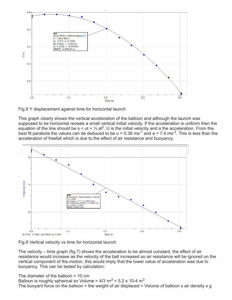
Fig.8 Y displacement against time for horizontal launch

This graph clearly shows the vertical acceleration of the balloon and although the launch wassupposed to be horizontal reveals a small vertical initial velocity. If the acceleration is uniform then theequation of the line should be s = ut + ½ at . U is the initial velocity and a the acceleration. From thebest fit parabola the values can de deduced to be u = 0.38 ms and a = 7.4 ms . This is less than theacceleration of freefall which is due to the effect of air resistance and buoyancy.

Fig.9 Vertical velocity vs time for horizontal launch

The velocity – time graph (fig.7) shows the acceleration to be almost constant, the effect of airresistance would increase as the velocity of the ball increased so air resistance will be ignored on thevertical component of the motion, this would imply that the lower value of acceleration was due tobuoyancy. This can be tested by calculation:

The diameter of the balloon = 10 cm Balloon is roughly spherical so Volume = 4/3 πr = 5.2 x 10­4 m The buoyant force on the balloon = the weight of air displaced = Volume of balloon x air density x g

2­1 ­2

3 3

3

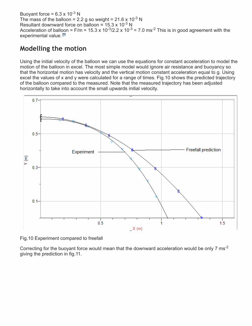
Buoyant force = 6.3 x 10 N The mass of the balloon = 2.2 g so weight = 21.6 x 10 N Resultant downward force on balloon = 15.3 x 10 N Acceleration of balloon = F/m = 15.3 x 10 /2.2 x 10 = 7.0 ms This is in good agreement with theexperimental value.

Modelling the motion

Using the initial velocity of the balloon we can use the equations for constant acceleration to model themotion of the balloon in excel. The most simple model would ignore air resistance and buoyancy sothat the horizontal motion has velocity and the vertical motion constant acceleration equal to g. Usingexcel the values of x and y were calculated for a range of times. Fig.10 shows the predicted trajectoryof the balloon compared to the measured. Note that the measured trajectory has been adjustedhorizontally to take into account the small upwards initial velocity.

Fig.10 Experiment compared to freefall

Correcting for the buoyant force would mean that the downward acceleration would be only 7 msgiving the prediction in fig.11.

­3­3

­3­3 ­3 ­2

­2

Fig.11 experiment compared to freefall and with the addition of buoyancy

This can be seen to give a slightly worse prediction since the time of flight is longer due to the reducedacceleration.

This final prediction was made by reducing the horizontal component of velocity by an amount thatwas proportional to the previous velocity this models the drag force which is proportional to thevelocity.

Fig.12 Experiment compared to model including Buoyancy and drag

The spreadsheet used to generate the data is shown below

Velocity is calculated with the formula =A2­C$12*A2 so each subsequent value is less than theprevious by an amount dependent on the constant in cell C12. The X displacement is then calculatedbased on this value. Each step of the motion calculated using the new velocity added on to theprevious displacement. The formula used to calculate the second step was =A3*0.05+C2, this is thetime interval multiplied by the new velocity plus the previous displacement. The constant was thenadjusted until the maximum x displacement was as in the experiment. The value 0.7 gave areasonably close fit.

Note: Only the freefall prediction is a quadratic best fit, all the others are cubic which gave a muchbetter fit for the range but probably wasn’t the actual equation of the line.

Conclusion and Evaluation

The aim of this investigation was to investigate the projectile motion of a small balloon. Bymeasurement and comparing with a theoretical model it was found that the motion of the balloon isaffected by both buoyancy and drag. Buoyancy reduces the vertical acceleration to a constant 7 ms .If this were the only effect the range of the balloon would be more than if in freefall but experimentshows it is less. The effect of drag compensates for the reduced acceleration so that the balloon doesnot travel as far as if in freefall.

The way that drag was modelled was based on the knowledge that the drag force is proportional to thevelocity so for each 0.05 s step in the model the velocity was reduced by an amount proportional tothe previous velocity. This is a simplification of the real situation but gave a very good prediction of theexperimental result.

The distance travelled by the balloon is quite short so the vertical velocity didn’t reach a very highvalue (the final vertical velocity was less than the initial horizontal velocity), had it travelled further thedrag force would have to be taken into account in the vertical component as well.

Although only one flight of the ball was mentioned many videos were made however the difficulty inachieving the same initial velocity made it pointless to try and combine multiple runs. Given more timeit would be beneficial to analyse more runs comparing each run to the model.

The main weakness in the method was the poor quality of the video, with a better camera with moreframes per second and a clearer picture the marking of the ball in LoggerPro would have been muchmore precise.

One surprise result was how little of the elastic energy was converted into kinetic, as the rubberreturns to its original shape some work is done on the gas, maybe this would give a measurable

­2

change in temperature. This loss of energy is in some way not so surprising since the effort required tostretch the rubber is much more than the effort required to make the ball travel the same distance byhitting it.

The original intention was to analyse the motion of the balloon launched at different angles howeverthis has been left for another time. Another interesting extension would be to change size of theballoon to increase the buoyant and drag forces. Keeping the size constant but changing the gas to amixture of air and Helium would enable the effect of buoyancy to be investigated further.

ù9ǃ

TwitterFacebookLinkedInÈGoogle +ÓEmail

Ûĝ

All materials on this website are for the exclusive use of teachers and students at subscribing schools for the period of their subscription. Anyunauthorised copying or posting of materials on other websites is an infringement of our copyright and could result in your account being blockedand legal action being taken against you.