ICES REPORT 12-03

January 2012

Isogeometric Divergence-conforming B-splines for theDarcy-Stokes-Brinkman Equations

by

John A. Evans and Thomas J.R. Hughes

The Institute for Computational Engineering and SciencesThe University of Texas at AustinAustin, Texas 78712

Reference: John A. Evans and Thomas J.R. Hughes, Isogeometric Divergence-conforming B-splines for theDarcy-Stokes-Brinkman Equations, ICES REPORT 12-03, The Institute for Computational Engineering andSciences, The University of Texas at Austin, January 2012.

Isogeometric Divergence-conforming B-splinesfor the Darcy-Stokes-Brinkman Equations

John A. Evans a,* and Thomas J.R. Hughes a

a Institute for Computational Engineering and Sciences, The University of Texas at Austin,∗ Corresponding author. E-mail address: evans@ices.utexas.edu

Abstract

We develop divergence-conforming B-spline discretizations for the numerical solutionof the Darcy-Stokes-Brinkman equations. These discretizations are motivated by therecent theory of isogeometric discrete differential forms and may be interpreted assmooth generalizations of Raviart-Thomas elements. The new discretizations are (atleast) patch-wise C0 and can be directly utilized in the Galerkin solution of Darcy-Stokes-Brinkman flow for single-patch configurations. When applied to incompress-ible flows, these discretizations produce pointwise divergence-free velocity fields andhence exactly satisfy mass conservation. In the presence of no-slip boundary condi-tions and multi-patch geometries, the discontinuous Galerkin framework is invokedto enforce tangential continuity without upsetting the conservation or stability prop-erties of the method across patch boundaries. Furthermore, as no-slip boundaryconditions are enforced weakly, the method automatically defaults to a compatiblediscretization of Darcy flow in the limit of vanishing viscosity. The proposed dis-cretizations are extended to general mapped geometries using divergence-preservingtransformations. For sufficiently regular single-patch solutions, we prove a priori er-ror estimates which are optimal for the discrete velocity field and suboptimal, byone order, for the discrete pressure field. Our estimates are additionally robust withrespect to the parameters of the Darcy-Stokes-Brinkman problem. We present a com-prehensive suite of numerical experiments which indicate optimal convergence ratesfor both the discrete velocity and pressure fields for general configurations, suggestingthat our a priori estimates may be conservative. The focus of the current paper isstrictly on incompressible flows, but our theoretical results naturally extend to flowscharacterized by mass sources and sinks.

Keywords: Darcy-Stokes-Brinkman equations, Generalized Stokes equations, B-splines,Isogeometric analysis, Divergence-conforming discretizations

1

1 Introduction

The Stokes equations describe a wide variety of fluid flows where advective inertialforces are so small when compared with viscous forces that they can be neglectedaltogether. Such flows arise in a large number of applications in nature and technol-ogy, from the flow of lava in the Earth’s mantle [54] to microfluidic flow in micro-electromechanical devices [41]. The Darcy-Stokes-Brinkman equations are a simpleextension of the Stokes equations which account for Darcy drag forces in highly porousmedia [13]. These equations, also referred to as the generalized Stokes equations, havebeen used to model groundwater flow [22], heat and mass transfer in pipes [39], andflow in biological tissues [40]. One also obtains a generalized Stokes problem whennonlinear terms are treated explicitly during semi-implicit time-integration of theunsteady Navier-Stokes equations.

Despite their simple appearance, the Stokes and generalized Stokes equations havepresented considerable difficulty in their numerical approximation. At the heart ofthe matter is the celebrated Babuska-Brezzi inf-sup condition [3, 12]. Simply put, thecondition states that one must properly select discrete velocity and pressure spacesin order to arrive at a stable and convergent discrete mixed formulation. Since theinception of the Marker-and-Cell scheme in 1965 [34], a large number of finite dif-ference, finite volume, and finite element methods have been devised to address thediscrete inf-sup condition in the context of the Stokes equations. For reference, seethe review by Boffi, Brezzi, and Fortin [9]. Most methods for Stokes flow only satisfythe incompressibility constraint in an approximate sense. Some bypass the inf-supcondition entirely through the use of a stabilized Petrov-Galerkin method [27]. How-ever, methods which return discretely divergence-free velocity fields are generally notrobust in the limit of vanishing viscosity when applied to generalized Stokes flows[45]. Moreover, mass conservation is considered to be of prime importance for cou-pled flow-transport [46], and it has been demonstrated that methods which fail toexactly satisfy the incompressibility constraint suffer from spurious velocity oscilla-tions when applied to “high pressure, low flow” problems [28, 44]. These issues havemotivated the development of discretization procedures which satisfy the incompress-ibility constraint exactly.

One of the simplest methods returning a divergence-free velocity field is thePk − P k−1 triangular element which approximates velocity fields using continuouspiecewise polynomials of degree k and pressure fields using discontinuous polynomi-als of degree k − 1. This method satisfies the Babuska-Brezzi condition for meshescontaining no nearly-singular vertices provided k ≥ 4 [53] and for certain macro-element configurations [2, 63]. Unfortunately, the method is not stable for generalmeshes and polynomial degrees. Recently, the use of H(div; Ω) elements has arisenas a new paradigm for the the simulation of generalized Stokes flows [38, 42, 61]. Asthese approximations are typically not members of H1(Ω), techniques such as theinterior penalty method [1, 24, 62] must be employed to enforce tangential continu-

2

ity across elements. Alternatively, one can modify divergence-conforming elementsto ensure they have some limited tangential continuity [56], and some authors haveelected to release continuity entirely in favor of hybridization [18, 17]. In the samevein, divergence-free wavelets have been proposed for the solution of Stokes flows[43, 58, 59, 55], though these discretizations have a complicated construction and areentirely limited to periodic and cuboidal domains.

In this paper, we present new divergence-conforming B-spline discretizations forthe generalized Stokes problem. These discretizations are motivated by the theory ofisogeometric discrete differential forms [15, 16] and may be interpreted as smooth gen-eralizations of Raviart-Thomas elements [49]. The new discretizations are (at least)patch-wise C0 and hence can be directly used in the Galerkin solution of generalizedStokes flow for single-patch configurations. We enforce no-slip boundary conditionsweakly by means of Nitsche’s method [48], allowing our method to default to a com-patible discretization of Darcy flow in the limit of vanishing viscosity. Alternativeinf-sup stable treatments of no-slip boundary conditions have been investigated inthe context of Stokes flow in [14]. In the presence of multi-patch geometries, we in-voke the discontinuous Galerkin framework in order to enforce tangential continuityacross patch interfaces while maintaining the stability and conservation propertiesof the method. The proposed discretizations are extended to general mapped ge-ometries using divergence- and integral-preserving transformations. For single-patchsolutions, we are able to prove robust a priori error estimates which are optimalfor the discrete velocity field and suboptimal, by one order, for the discrete pressurefield. This is reminiscent of error estimates for stabilized equal-order interpolationsof the Stokes equations [27, 37]. Our derived estimates are also robust with respectto the parameters of generalized Stokes flow. We utilize the methods of exact andmanufactured solutions to validate our estimates, and we find that pressure actuallyconverges at optimal order. We further test the effectiveness of our method using acollection of benchmark problems: two-dimensional creeping lid-driven cavity flow,three-dimensional creeping lid-driven cavity flow, and Darcy-dominated generalizedStokes flow subject to boundary layers.

An outline of this paper is as follows. In the following section, we present somebasic notation. In Section 3, we recall the generalized Stokes problem subject to ho-mogeneous boundary conditions. In Section 4, we briefly review B-splines, the basicbuilding blocks of our new discretization technique, and in Section 5, we define the B-spline spaces which we will utilize to discretize velocity and pressure fields. In Section6, we present our discrete variational formulation for the generalized Stokes problemand prove continuity, stability, and a priori error estimates for the single-patch set-ting. In Section 7, we discuss how to extend our methodology to the multi-patchsetting. In Sections 8 and 9, we present numerical results, and in Section 10, we drawconclusions. Throughout this paper, we make explicit all of our estimates’ dependen-cies on the problem parameters as well as the penalty parameter of Nistche’s method.This will require a lengthy and tedious analysis, but we believe that knowledge of

3

such dependencies is of great practical importance. Additionally, the focus of thispaper is strictly on incompressible flows. Our theoretical results naturally extend toflows characterized by mass sources and sinks.

2 Notation

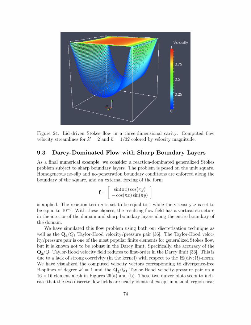
We begin this paper with some basic notation. For d a positive integer representingdimension, let D ⊂ Rd denote an arbitrary bounded Lipschitz domain with boundary∂D. As usual, let L2(D) denote the space of square integrable functions on D and

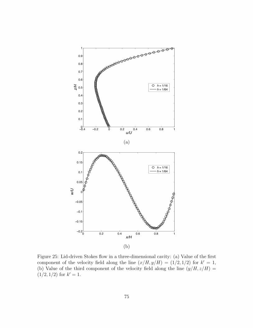
define L2(D) = (L2(D))d. We will also utilize the more general Lebesgue spaces

Lp(D) where 1 ≤ p ≤ ∞ and their vectorial counterpart Lp(D). Let Hk(D) denotethe space of functions in L2(D) whose kth-order derivatives belong to L2(D) and

define Hk(D) =(Hk(D)

)d. We identify with Hk(D) the standard Sobolev norm

‖v‖Hk(D) =

∑|α|<k

‖Dαv‖2L2(D)

1/2

where α = (α1, α2, . . . , αd) is a multi-index of non-negative integers, |α| = α1 + α2 +. . .+ αd, and

Dα =∂|α|

∂xα11 ∂x

α22 . . . ∂xαd

d

.

We denote the Sobolev semi-norms as | · |Hk(D), and we use the convention H0(D) =L2(D). Throughout, Sobolev spaces of fractional order are defined using functionspace interpolation (see, e.g., Chapter 1 of [57]). We define H1

0 (D) ⊂ H1(D) to bethe subspace of functions with homogeneous boundary conditions and define H1

0(D)to be the vectorial counterpart of H1

0 (D). We define Hs(div;D) to be the Sobolevspace of all functions in Hs(Ω) whose divergence also belongs to Hs(D). This spaceis equipped with the norm

‖v‖Hs(div;D) =(‖v‖2

Hs(D) + ‖divv‖2Hs(D)

)1/2.

When s = 0, we drop the index. We also define

H0(div;D) = v ∈ H(div;D) : v · n = 0 on ∂D

where n denotes the outward pointing unit normal. Finally, we denote L20(D) ⊂ L2(D)

as the space of square-integrable functions with zero average on D.

3 The Generalized Stokes Problem

In this section, we recall the generalized Stokes problem subject to homogeneousDirichlet boundary conditions. For d a positive integer, let Ω denote a Lipschitz

4

bounded open set of Rd. Throughout this paper, d will be either 2 or 3. The problemof interest is as follows.

(S)

Given σ : Ω→ R, ν : Ω→ R, and f : Ω→ Rd, find u : Ω→ Rd and p : Ω→ Rsuch that

σu−∇ · (2ν∇su) + gradp = f in Ω (1)

divu = 0 in Ω (2)

u = 0 on ∂Ω. (3)

Above, u denotes the flow velocity of a fluid moving through the domain Ω, p denotesthe pressure acting on the fluid divided by the fluid density, ν denotes the kinematicviscosity of the fluid, σ denotes the reaction coefficient which gives the ratio of theviscosity to the permeability of the fluid, and f denotes a body force acting on thefluid divided by the density. We assume that the viscosity is taken to be uniformlypositive (i.e., ∃ν0 > 0 such that ν ≥ ν0) and that the reaction coefficient is taken tobe non-negative (i.e., σ ≥ 0). Note that the pressure is only determined up to anarbitrary constant.

Let us now make an assumption regarding the data of our problem. Notably, letus assume that σ, ν ∈ L∞(Ω) and f ∈ L2(Ω) . The weak form for the generalizedStokes problem is then written as follows:

(W )

Find u ∈ H10(Ω) and p ∈ L2

0(Ω) such that

a(u,v)− b(p,v) + b(q,u) = (f,v)L2(Ω) (4)

for all v ∈ H10(Ω) and q ∈ L2

0(Ω) where

a(w,v) = (2ν∇sw,∇sv)(L2(Ω))d×d + (σw,v)L2(Ω) , ∀w,v ∈ H10(Ω) , (5)

b(q,v) = (q, divv)L2(Ω) , ∀q ∈ L20(Ω),v ∈ H1

0(Ω) . (6)

We have the following theorem which is a simple consequence of coercivity, continuity,and a continuous inf-sup condition.

Theorem 3.1. Problem (W ) has a unique weak solution (u, p) ∈ H10(Ω) × L2

0(Ω).

4 B-splines and Geometrical Mappings

In this section, we briefly introduce B-splines, the primary ingredient in our dis-cretization technique for the generalized Stokes equations. We also introduce map-pings which will allow us to extend our discretization technique to general geometries

5

of engineering interest. For an overview of B-splines, their properties, and robust al-gorithms for evaluating their values and derivatives, see de Boor [23] and Schumaker[52]. For the application of B-splines to finite element analysis, see Hollig [35] andCottrell, Hughes, and Bazilevs [20].

4.1 Univariate B-splines

For two positive integers k and n, representing degree and dimensionality respectively,let us introduce the ordered knot vector

Ξ := 0 = ξ1, ξ2, . . . , ξn+k+1 = 1 (7)

whereξ1 ≤ ξ2 ≤ . . . ξn+k+1.

Given Ξ and k, univariate B-spline basis functions are constructed recursively startingwith piecewise constants (k = 0):

B0i (ξ) =

1 if ξi ≤ ξ < ξi+1

0 otherwise.(8)

For k = 1, 2, 3, . . ., they are defined by

Bki (ξ) =

ξ − ξiξi+k − ξi

Bk−1i (ξ) +

ξi+k+1 − ξξi+k+1 − ξi+1

Bk−1i+1 (ξ). (9)

When ξi+k − ξi = 0, ξ−ξiξi+k−ξi

is taken to be zero, and similarly, when ξi+k+1− ξi+1 = 0,ξi+k+1−ξ

ξi+k+1−ξi+1is taken to be zero. B-spline basis functions are piecewise polynomials of

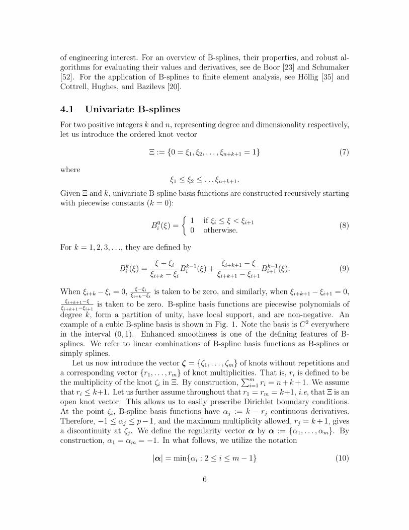
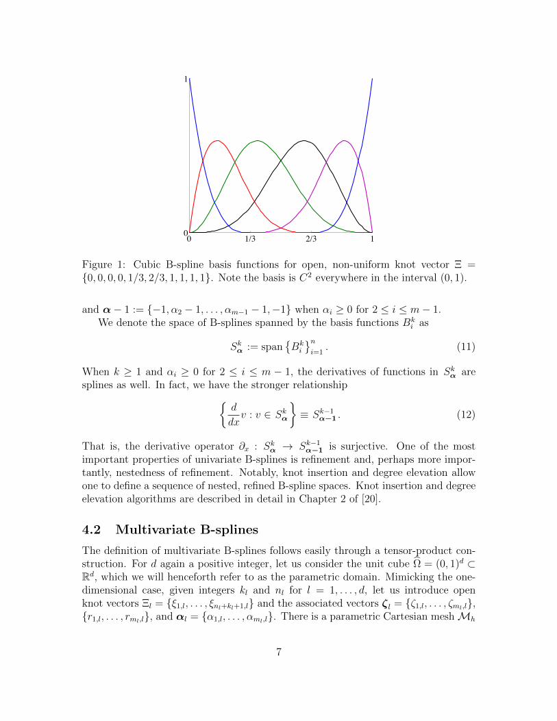
degree k, form a partition of unity, have local support, and are non-negative. Anexample of a cubic B-spline basis is shown in Fig. 1. Note the basis is C2 everywherein the interval (0, 1). Enhanced smoothness is one of the defining features of B-splines. We refer to linear combinations of B-spline basis functions as B-splines orsimply splines.

Let us now introduce the vector ζ = ζ1, . . . , ζm of knots without repetitions anda corresponding vector r1, . . . , rm of knot multiplicities. That is, ri is defined to bethe multiplicity of the knot ζi in Ξ. By construction,

∑mi=1 ri = n+k+ 1. We assume

that ri ≤ k+1. Let us further assume throughout that r1 = rm = k+1, i.e, that Ξ is anopen knot vector. This allows us to easily prescribe Dirichlet boundary conditions.At the point ζi, B-spline basis functions have αj := k − rj continuous derivatives.Therefore, −1 ≤ αj ≤ p− 1, and the maximum multiplicity allowed, rj = k+ 1, givesa discontinuity at ζj. We define the regularity vector α by α := α1, . . . , αm. Byconstruction, α1 = αm = −1. In what follows, we utilize the notation

|α| = minαi : 2 ≤ i ≤ m− 1 (10)

6

0 11/3 2/30

1

Figure 1: Cubic B-spline basis functions for open, non-uniform knot vector Ξ =0, 0, 0, 0, 1/3, 2/3, 1, 1, 1, 1. Note the basis is C2 everywhere in the interval (0, 1).

and α− 1 := −1, α2 − 1, . . . , αm−1 − 1,−1 when αi ≥ 0 for 2 ≤ i ≤ m− 1.We denote the space of B-splines spanned by the basis functions Bk

i as

Skα := spanBki

ni=1

. (11)

When k ≥ 1 and αi ≥ 0 for 2 ≤ i ≤ m − 1, the derivatives of functions in Skα aresplines as well. In fact, we have the stronger relationship

d

dxv : v ∈ Skα

≡ Sk−1

α−1 . (12)

That is, the derivative operator ∂x : Skα → Sk−1α−1 is surjective. One of the most

important properties of univariate B-splines is refinement and, perhaps more impor-tantly, nestedness of refinement. Notably, knot insertion and degree elevation allowone to define a sequence of nested, refined B-spline spaces. Knot insertion and degreeelevation algorithms are described in detail in Chapter 2 of [20].

4.2 Multivariate B-splines

The definition of multivariate B-splines follows easily through a tensor-product con-struction. For d again a positive integer, let us consider the unit cube Ω = (0, 1)d ⊂Rd, which we will henceforth refer to as the parametric domain. Mimicking the one-dimensional case, given integers kl and nl for l = 1, . . . , d, let us introduce openknot vectors Ξl = ξ1,l, . . . , ξnl+kl+1,l and the associated vectors ζl = ζ1,l, . . . , ζml,l,r1,l, . . . , rml,l, and αl = α1,l, . . . , αml,l. There is a parametric Cartesian meshMh

7

associated with these knot vectors partitioning the parametric domain into rectangu-lar parallelepipeds. Visually,

Mh = Q = ⊗l=1,...,d (ζil,l, ζil+1,l) , 1 ≤ il ≤ ml − 1 . (13)

For each element Q ∈ Mh we associate a parametric mesh size hQ = diam(Q). Wealso define a shape regularity constant λ which satisfies the inequality

λ−1 ≤ hQ,min

hQ≤ λ, ∀Q ∈Mh, (14)

where hQ,min denotes the length of the smallest edge of Q. A sequence of parametricmeshes that satisfy the above inequality for an identical shape regularity constant issaid to be locally quasi-uniform.

We associate with each knot vector Ξl (l = 1, . . . , d) univariate B-spline basisfunctions Bkl

il,lof degree kl for il = 1, . . . , nl. On the mesh Mh, we define the tensor-

product B-spline basis functions as

Bk1,...,kdi1,...,id

:= Bk1i1,1⊗ . . .⊗Bkd

id,d, i1 = 1, . . . , n1, . . . id = 1, . . . , nd. (15)

We then accordingly define the tensor-product B-spline space as

Sk1,...,kdα1,...,αd≡ Sk1,...,kdα1,...,αd

(Mh) := spanBk1,...,kdi1,...,id

n1,...,nd

i1=1,...,id=1. (16)

The space is fully characterized by the mesh Mh, the degrees kl, and the regularityvectors αl, as the notation reflects. Like their univariate counterparts, multivariateB-spline basis functions are piecewise polynomial, form a partition of unity, have localsupport, and are non-negative. Defining the regularity constant

α := minl=1,...,d

min2≤il≤ml−1

αil,l (17)

we see that our B-splines are Cα-continuous throughout the domain Ω. Refinement ofmultivariate B-spline bases is obtained by applying knot insertion and degree elevationin tensor-product fashion. In the remainder of the text, we consider a family ofnested meshes Mhh≤h0 and associated B-spline spaces

Sk1,...,kdα1,...,αd

(Mh)h≤h0

that

have been obtained by successive applications of knot refinement. Furthermore, weassume throughout that the mesh family Mhh≤h0 is locally quasi-uniform.

Note that each element Q = ⊗l=1,...,d (ζil,l, ζil+1,l) has the equivalent representationQ = ⊗l=1,...,d (ξjl,l, ξjl+1,l) for some index jl. With this in mind, we associate with eachelement a support extension Q, defined as

Q := ⊗l=1,...,d (ξjl−pl,l, ξjl+pl+1,l) . (18)

The support extension is the interior of the set formed by the union of the supportsof all B-spline basis functions whose support intersects Q. Note that each elementbelongs to the support extension of at most Πl=1,...,d(2pl + 1) elements. The supportextension is a natural object to consider when examining the local approximationproperties of a B-spline space.

8

4.3 Piecewise Smooth Functions, Geometrical Mappings, andPhysical Mesh Entities

On the parametric meshMh, we define the space of piecewise smooth functions withinterelement regularity given by the vectors α1, . . . ,αd as

C∞α1,...,αd= C∞α1,...,αd

(Mh) . (19)

Precisely, a function in C∞α1,...,αdis a function whose restriction to an element Q ∈Mh

admits a C∞ extension in the closure of that element and which has αil,l contin-uous derivatives with respect to the lth coordinate along the internal mesh faces(x1, . . . , xd) : xl = ζil,l, ζjl′ ,l′ < xl′ < ζjl′+1,l

′ , l′ 6= l for all il = 2, . . . ,ml − 1 andjl′ = 1, . . . ,ml′ − 1. Note immediately that any function lying in the B-spline spaceSk1,...,kdα1,...,αd

also lies in C∞α1,...,αd.

Unless specified otherwise, we assume throughout the rest of the paper that thephysical domain Ω ⊂ Rd can be exactly parametrized by a geometrical mapping

F : Ω → Ω belonging to(C∞α1,...,αd

)dwith piecewise smooth inverse. We further

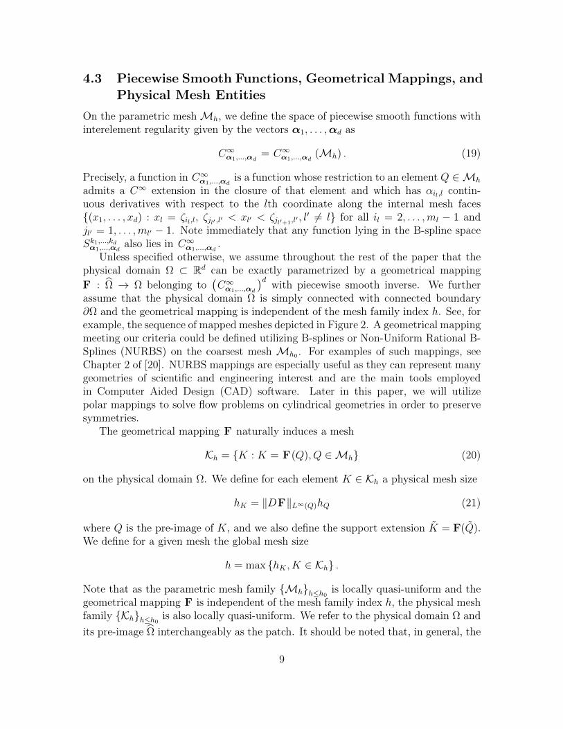
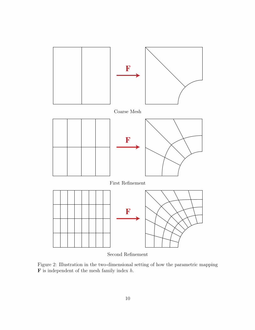
assume that the physical domain Ω is simply connected with connected boundary∂Ω and the geometrical mapping is independent of the mesh family index h. See, forexample, the sequence of mapped meshes depicted in Figure 2. A geometrical mappingmeeting our criteria could be defined utilizing B-splines or Non-Uniform Rational B-Splines (NURBS) on the coarsest mesh Mh0 . For examples of such mappings, seeChapter 2 of [20]. NURBS mappings are especially useful as they can represent manygeometries of scientific and engineering interest and are the main tools employedin Computer Aided Design (CAD) software. Later in this paper, we will utilizepolar mappings to solve flow problems on cylindrical geometries in order to preservesymmetries.

The geometrical mapping F naturally induces a mesh

Kh = K : K = F(Q), Q ∈Mh (20)

on the physical domain Ω. We define for each element K ∈ Kh a physical mesh size

hK = ‖DF‖L∞(Q)hQ (21)

where Q is the pre-image of K, and we also define the support extension K = F(Q).We define for a given mesh the global mesh size

h = max hK , K ∈ Kh .

Note that as the parametric mesh family Mhh≤h0 is locally quasi-uniform and thegeometrical mapping F is independent of the mesh family index h, the physical meshfamily Khh≤h0 is also locally quasi-uniform. We refer to the physical domain Ω and

its pre-image Ω interchangeably as the patch. It should be noted that, in general, the

9

F

Nih1wi

h1

W i 1,…,n1

Nih1wi

h1

WF 1

i 1,…,n1

Coarse Mesh

F

Nih2wi

h2

W i 1,…,n2

Nih2wi

h2

WF 1

i 1,…,n2

First Refinement

F

Nih3wi

h3

W i 1,…,n3

Nih3wi

h3

WoF 1

i 1,…,n3

Second Refinement

Figure 2: Illustration in the two-dimensional setting of how the parametric mappingF is independent of the mesh family index h.

10

domain Ω cannot be represented using just a single patch. Instead, multiple patchesmust be employed. We will discuss further the multi-patch setting in Section 7.

We define on the parametric mesh a set of mesh faces Fh = F where F is a faceof one or more elements in Mh. We define the physical set of mesh faces as

Fh = F = F(F ) : F ∈ Fh

and we define the boundary mesh to be

Γh = F ∈ Fh : F ⊂ ∂Ω .

By construction,∂Ω = ∪F∈Γh

F .

Note that for each face F ∈ Γh there is a unique K ∈ Kh such that F is a “face” ofK (in the sense that F is the image of a face of Q, the pre-image of K). We hencedefine for such a face the mesh size

hF := hK .

One may also define hF to be the wall-normal mesh-size as is done in [7]. Such adefinition is more appropriate when stretched meshes are utilized in the presence oflayers.

Throughout the paper, we will utilize the terminology “a constant independentof h”. When we employ such terminology, we simply indicate that the constantwill not depend on the given mesh and, in particular, its size. The constant may,however, depend on the domain, the shape regularity of the parametric mesh family,the polynomial degrees of the employed B-spline spaces, and global, mesh-invariantmeasures of the parametric mapping.

5 Discretization of Velocity and Pressure Fields

In this section, we define the B-spline spaces which we will utilize to discretize thevelocity and pressure fields appearing in the generalized Stokes problem. These spacesare motivated by the recent theory of isogeometric discrete differential forms [15, 16]and may be interpreted as smooth generalizations of Raviart-Thomas elements [49].We first define our discrete velocity and pressure spaces on the parametric domainΩ = (0, 1)d and then define discrete spaces on the physical domain Ω using divergence-and integral-preserving transformations. We finish this section with a presentationof local approximation estimates and trace inequalities for our discrete velocity andpressure spaces.

11

5.1 Discrete Spaces on the Parametric Domain

Using the notation of the previous section and assuming that

α := min|αl| : l = 1, . . . , d ≥ 1,

we define the following two spaces:

Vh :=

Sk1,k2−1α1,α2−1 × S

k1−1,k2α1−1,α2

if d = 2,

Sk1,k2−1,k3−1α1,α2−1,α3−1 × S

k1−1,k2,k3−1α1−1,α2,α3−1 × S

k1−1,k2−1,k3α1−1,α2−1,α3

if d = 3,

Qh :=

Sk1−1,k2−1α1−1,α2−1 if d = 2,

Sk1−1,k2−1,k3−1α1−1,α2−1,α3−1 if d = 3.

The space Vh comprises our set of discrete velocity fields while Qh comprises ourset of discrete pressure fields. Note that as α ≥ 1, our discrete velocity fields areH1-conforming. If we allow α = 0, our spaces collapse to standard Raviart-Thomasmixed finite elements [49]. In order to deal with no-penetration boundary conditions,we make use of the following constrained discrete spaces:

V0,h :=

vh ∈ Vh : vh · n = 0 on ∂Ω,

Q0,h :=

qh ∈ Qh :

∫Ω

qhdx = 0

.

Above, n denotes the outward-facing normal to ∂Ω. As specified in the introduction,we choose to enforce no-slip boundary condition weakly using Nitsche’s method [48].

Due to the special relationship given by (12), the spaces V0,h and Q0,h along with theparametric divergence operator form the bounded discrete cochain complex

V0,hdiv−−−→ Q0,h

where div is the divergence operator on the unit cube Ω. In fact, we have a muchstronger result due to the results of [15].

Proposition 5.1. There exist L2-stable projection operators Π0Vh

: H0(div; Ω) → V0,h

and Π0Qh

: L20(Ω)→ Q0,h such that the following diagram commutes:

H0(div; Ω)div−−−→ L2

0(Ω)

Π0Vh

y Π0Qh

yV0,h

div−−−→ Q0,h.

(22)

Furthermore, there exists a positive constant Cu independent of h such that

‖Π0Vh

v‖H1(Ω) ≤ Cu‖v‖H1(Ω), ∀v ∈ H0(div; Ω) ∩ H1(Ω) . (23)

12

5.2 Discrete Spaces on the Physical Domain

To define our discrete velocity and pressure spaces on the physical domain, we intro-duce the following pullback operators:

ιu(v) := det (DF) (DF)−1 (v F) , v ∈ H0(div; Ω) (24)

ιp(q) := det (DF) (q F) , q ∈ L20(Ω) (25)

where DF is the Jacobian matrix of the parametric mapping F. The push-forwardgiven by (24), popularly known as the Piola transform, has two important properties:(i) it preserves the nullity of normal components, (ii) it maps divergences to diver-gences. Hence, it maps divergence-free fields in parametric space to divergence-freefields in physical space, as illustrated in Fig. 3. On the other hand, the push-forwardgiven by (25) has the property that it preserves the nullity of the integral operator.Due to these properties, we have the following commuting diagram:

H0(div; Ω)div−−−→ L2

0(Ω)

ιu

x ιp

xH0(div; Ω)

div−−−→ L20(Ω).

(26)

This motivates the use of the following discrete velocity and pressure spaces in thephysical domain:

V0,h :=

v ∈ H0(div; Ω) : ιu(v) ∈ V0,h

,

Q0,h :=q ∈ L2

0(Ω) : ιp(q) ∈ Q0,h

.

Furthermore, we define the projectors Π0Vh : H0(div; Ω) → V0,h and Π0

Qh: L2(Ω) →

Q0,h via the compositions

Π0Qh

:= ι−1u Π0

Qh ιu, Π0

Qh:= ι−1

p Π0Qh ιp.

Employing the preceding results and terminology as well as the smoothness propertiesof the parametric mapping F , we arrive at the following proposition.

Proposition 5.2. The following diagram commutes:

H0(div; Ω)div−−−→ L2

0(Ω)

Π0Vh

y Π0Qh

yV0,h

div−−−→ Q0,h.

(27)

Furthermore, there exists a positive constant Cu independent of h such that

‖Π0Vh v‖H1(Ω) ≤ Cu‖v‖H1(Ω), ∀v ∈ H0(div; Ω) ∩ H1(Ω) . (28)

13

Compatible B-splines

Two-dimensional Compatible B-splines:

NURBS Mapped Domains

On NURBS mapped domains, the Piola transform is utilized

to map flow velocities. Pressures are mapped using an

integral preserving transform.

Figure 3: The Piola transform maps divergence-free fields in parametric space todivergence-free fields in physical space, as shown here for the case of a divergence-freeB-spline.

We immediately have an inf-sup condition for our discrete velocity/pressure pair.

Proposition 5.3. There exists a positive constant β independent of h such that thefollowing holds: for every qh ∈ Q0,h, there exists a vh ∈ V0,h such that:

divvh = qh (29)

and‖vh‖H1(Ω) ≤ β−1‖qh‖L2(Ω). (30)

Hence,

infqh∈Q0,h

qh 6=0

supvh∈V0,h

(divvh, qh)L2(Ω)

‖vh‖H1(Ω)‖qh‖L2(Ω)

≥ β. (31)

Proof. Let qh ∈ Q0,h be arbitrary. It is a classical result (see pg. 24 of [29], forexample) that there exists a function v ∈ H1

0(Ω) such that divv = qh and

‖v‖H1(Ω) ≤ β−1‖qh‖L2(Ω)

where β is a positive constant independent of v. Let vh = Π0Vh v. Then, by Proposi-

tion 5.2, divvh = div Π0Vh v = Π0

Qhdivv = qh and

‖vh‖H1(Ω) ≤ Cu‖v‖H1(Ω) ≤ Cuβ−1‖qh‖L2(Ω).

Thus the theorem holds with β = βCu

.

14

We would like to state that such an inf-sup condition would not have held if wehad elected to strongly enforce homogeneous tangential boundary conditions withinthe space V0,h. This is because

divV0,h ∩ H1

0(Ω)( Q0,h.

Hence, there exists a qh ∈ Q0,h such that qh 6= 0 and

supvh∈V0,h∩H1

0(Ω)

(divvh, qh)L2(Ω)

‖vh‖H1(Ω)‖qh‖L2(Ω)

= 0.

Hence, an alternative methodology must be employed if one wishes to strongly enforcehomogeneous tangential boundary conditions within the space V0,h. For example, in[14], a special discrete pressure space was constructed in the two-dimensional settingby selectively reducing the dimensionality ofQ0,h using T-splines [5]. However, a proofof mesh-independent discrete stability remains absent with this choice of pressurespace, and the convenient tensor-product structure of B-splines is lost.

We also have the following result.

Proposition 5.4. If vh ∈ V0,h satisfies

(divvh, qh)L2(Ω) = 0, ∀qh ∈ Q0,h, (32)

then divvh ≡ 0.

Proof. The proof holds trivially as div maps V0,h onto Q0,h.

Hence, by choosing V0,h and Q0,h as discrete velocity and pressure spaces, wearrive at a discretization that automatically returns velocity fields that are pointwisedivergence-free.

5.3 Visualization of Basis Functions

We now visualize some of the basis functions associated with our chosen discretevelocity and pressure spaces. For ease of presentation, we confine ourselves to thetwo-dimensional setting. We also work with the unconstrained analogues of V0,h andQ0,h, which we denote as Vh and Qh. Let k1 = k2 = 2, and let Ξ1 and Ξ2 be equal to

Ξ1 := Ξ2 := 0, 0, 0, 1/3, 2/3, 1, 1, 1 .

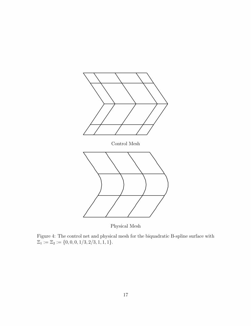
These polynomial degrees and knot vectors define a parametric meshMh and B-splinespaces Vh and Qh overMh. To define the physical domain, we employ a biquadratic B-spline mapping. The control net defining this mapping (see Chapter 2 of [20]) and theresulting physical mesh Kh are illustrated in Figure 4. In Figure 5, we have depicted

15

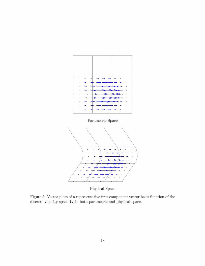
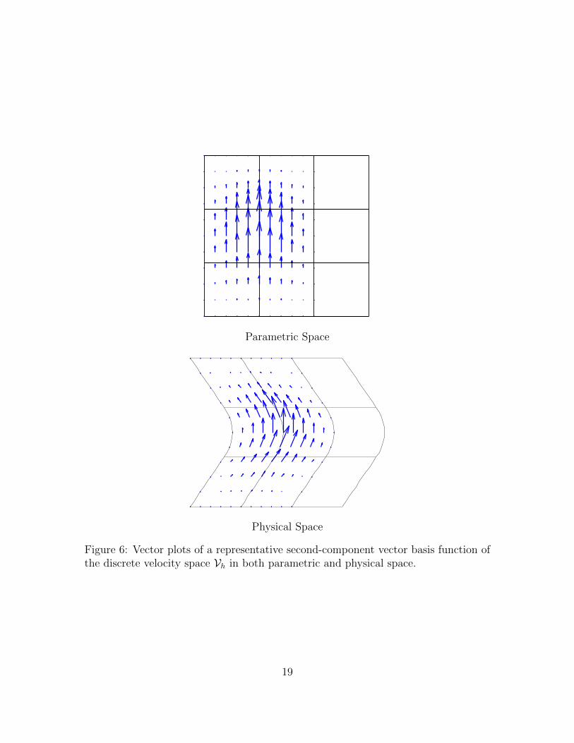
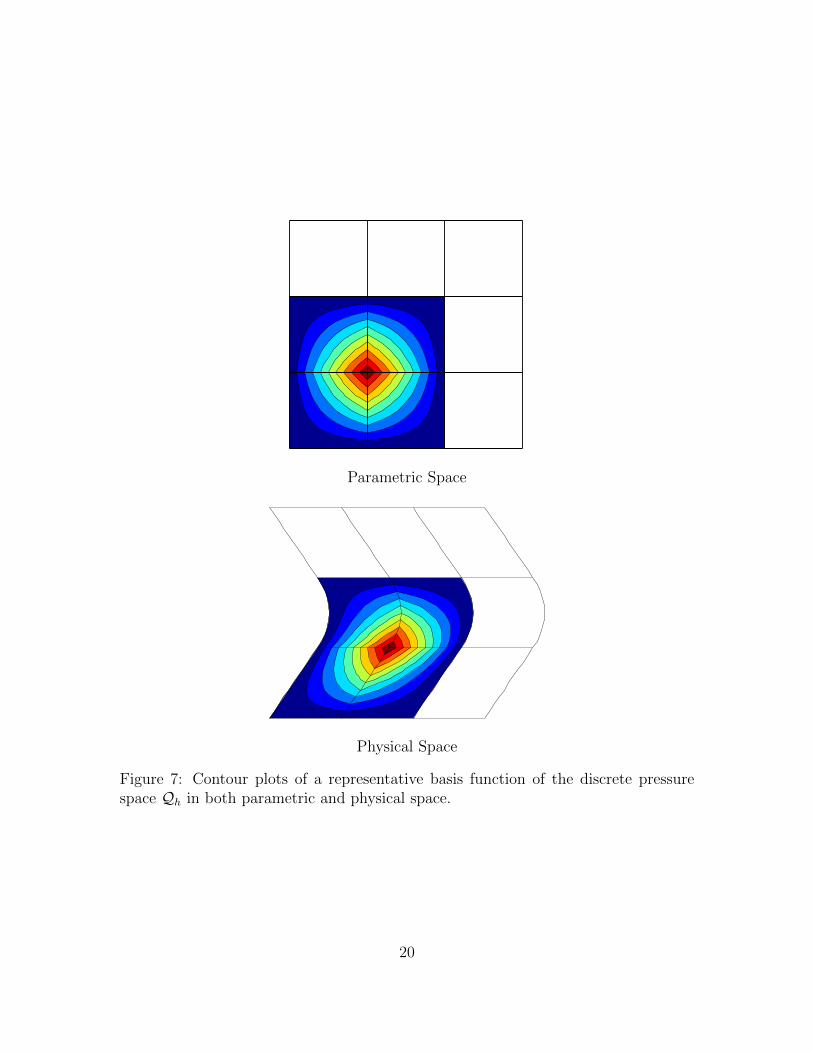
a “first-component” vector basis function of the discrete velocity space Vh. Notethat the basis function is C1-continuous along horizontal parametric lines and C0-continuous along vertical parametric lines. Further note that the directionality of thebasis function is preserved under the map ιu in the sense that the function is orientedin the direction of horizontal parametric lines in both parametric and physical space.In Figure 6, we have depicted a typical “second-component” vector basis function ofVh. Note that the basis function is C0-continuous along horizontal parametric linesand C1-continuous along vertical parametric lines, and the directionality of the basisfunction is preserved under the map ιu in the sense that the function is oriented in thedirection of vertical parametric lines in both parametric and physical space. Finally,in Figure 7, we have depicted a representative basis function of the discrete pressurespace Qh which is C0-continuous in both parametric and physical space.

5.4 Approximation Results and Trace Inequalities

Let us definek′ = min

l=1,...,d|pl − 1| . (33)

Note that the discrete velocity and pressure spaces V0,h and Q0,h consist of mappedpiecewise polynomials which are complete up to degree k′. Hence, k′ may be thoughtof as the polynomial degree of our discretization technique. The following resultdetails the local approximation properties of our discrete spaces. Its proof may befound in [15].

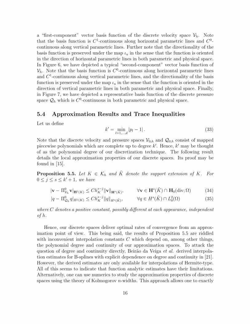
Proposition 5.5. Let K ∈ Kh and K denote the support extension of K. For0 ≤ j ≤ s ≤ k′ + 1, we have

|v− Π0Vh v|Hj(K) ≤ Chs−jK ‖v‖Hs(K), ∀v ∈ Hs(K) ∩ H0(div; Ω) (34)

|q − Π0Qhq|Hj(K) ≤ Chs−jK ‖q‖Hs(K), ∀q ∈ Hs(K) ∩ L2

0(Ω) (35)

where C denotes a positive constant, possibly different at each appearance, independentof h.

Hence, our discrete spaces deliver optimal rates of convergence from an approx-imation point of view. This being said, the results of Proposition 5.5 are riddledwith inconvenient interpolation constants C which depend on, among other things,the polynomial degree and continuity of our approximation spaces. To attack thequestion of degree and continuity directly, Beirao da Veiga et al. derived interpola-tion estimates for B-splines with explicit dependence on degree and continuity in [21].However, the derived estimates are only available for interpolations of Hermite-type.All of this seems to indicate that function analytic estimates have their limitations.Alternatively, one can use numerics to study the approximation properties of discretespaces using the theory of Kolmogorov n-widths. This approach allows one to exactly

16

Student Version of MATLAB

Control Mesh

Student Version of MATLAB

Physical Mesh

Figure 4: The control net and physical mesh for the biquadratic B-spline surface withΞ1 := Ξ2 := 0, 0, 0, 1/3, 2/3, 1, 1, 1.

17

Student Version of MATLAB

Parametric Space

Student Version of MATLAB

Physical Space

Figure 5: Vector plots of a representative first-component vector basis function of thediscrete velocity space Vh in both parametric and physical space.

18

Student Version of MATLAB

Parametric Space

Student Version of MATLAB

Physical Space

Figure 6: Vector plots of a representative second-component vector basis function ofthe discrete velocity space Vh in both parametric and physical space.

19

Student Version of MATLAB

Parametric Space

Student Version of MATLAB

Physical Space

Figure 7: Contour plots of a representative basis function of the discrete pressurespace Qh in both parametric and physical space.

20

compute the interpolation constants associated with variational projection throughthe solution of a generalized eigenproblem. The theory of Kolmogorov n-widths wasused to study one-dimensional B-spline discretizations in [25]. This paper revealedthat maximal continuity B-spline spaces harbor nearly optimal resolution propertiesand admit smaller intepolation constants than lower continuity spaces. Recently,the theory of Kolmogorov n-widths has been used to study multi-dimensional andcompatible B-spline discretizations. This study has also revealed the advantage ofemploying B-splines of maximal continuity in the multi-dimensional setting. Theresults of this study will be presented in a forthcoming publication.

We will also need the following trace estimate in our proceeding mathematicalanalysis. Its proof can be found in [26].

Proposition 5.6. Let K ∈ Kh and Q = F−1(K). Then we have

‖ (∇svh) n‖(L2(∂K))d ≤ Ctraceh−1K ‖vh‖H1(K), ∀vh ∈ V0,h (36)

where Ctrace denotes a positive constant independent of h.

In [26], it was shown that Proposition 5.6 holds with Ctrace ∼ (k′)2. However, ournumerical experience has indicated that a corresponding global trace inequality holdswith Ctrace ∼ k′ if B-splines of maximal continuity are utilized. This allows us toselect a smaller penalty parameter when employing Nitsche’s method. As we will seein the next section, our convergence estimates scale inversely with the square root ofNitsche’s penalty parameter. Hence, we want to select Nitsche’s penalty parameteras small as possible.

6 Approximation of the Generalized Stokes Prob-

lem

In this section, we approximate the homogeneous generalized Stokes problem usingthe discrete velocity and pressure spaces introduced in the previous section. We provecontinuity, stability, and a priori error estimates for our discretization scheme in thesingle patch setting, and we explicitly track all of our estimates’ dependencies on theproblem parameters and Nitsche’s penalty parameter.

6.1 Variational Formulation

We begin this section by presenting a discrete variational formulation for the gener-alized Stokes problem. Since members of V0,h do not satisfy homogeneous tangentialDirichlet boundary conditions, we resort to Nitsche’s method [48] to weakly enforceno-slip boundary conditions. This requires slightly more regularity on our problemdata. Specifically, we assume

ν ∈ W 1,∞(Ω) := w ∈ L∞(Ω) : ∇w ∈ L∞(Ω) .

21

This assumption ensures the trace of ν on the boundary ∂Ω is well-defined. Now, letus define the following bilinear form:

ah(w,v) = a(w,v)−∑F∈Γh

∫F

2ν

(((∇sv) n) ·w + ((∇sw) n) · v− Cpen

hFw · v

)ds.

(37)In the above equation, Cpen ≥ 1 denotes a specially chosen positive penalty constantwhich will be specified in the sequel. Our discrete formulation is written as follows.

(G)

Find uh ∈ V0,h and ph ∈ Q0,h such that

ah(uh,vh)− b(ph,vh) + b(qh,uh) = (f,vh)L2(Ω) ,

∀vh ∈ V0,h, qh ∈ Q0,h. (38)

Note that the mesh-dependent bilinear form given by (37) has three additional termsin comparison with the continuous bilinear form: a penalty term, a consistency term,and a stability term. All three of these terms will prove important in our proceedingmathematical analysis.

We have the following lemma detailing the consistency of our numerical methodprovided the exact solution satisfies a reasonable regularity condition.

Lemma 6.1. Suppose that the unique weak solution (u, p) of (W ) satisfies the regu-larity condition u ∈ H3/2+ε(Ω) for some ε > 0. Then:

ah(u,vh)− b(p,vh) + b(qh,u) = (f ,vh)L2(Ω) (39)

for all vh ∈ V0,h and qh ∈ Q0,h.

Proof. We trivially haveb(qh,u) = 0, ∀qh ∈ Q0,h.

Now let vh ∈ V0,h. By the trace theorem for fractional Sobolev spaces [57], theassumption u ∈ H3/2+ε(Ω) guarantees that (∇su) n is well-defined along ∂Ω and(∇su) n ∈ (L2(∂Ω))d. Furthermore, (∇svh) n is well-defined along ∂Ω and (∇svh) n ∈(L2(∂Ω))d. Hence, the quantity ah(u,vh) is well-defined. Utilizing integration byparts and the fact that u satisfies homogeneous Dirichlet boundary conditions andvh satisfies homogeneous normal Dirichlet boundary conditions, we have

ah(u,vh)− b(p,vh) =

∫Ω

(σu−∇ · (2ν∇su) + gradp) · vhdx

=

∫Ω

f · vhdx

= (f,vh)L2(Ω)

where integration is to be understood in the sense of distributions. This completesthe proof of the lemma.

22

Consistency is the primary reason that we employed Nitsche’s method instead of anaıve penalty method. Nitsche’s method also admits adjoint consistency, and this willallow us to prove optimal L2 estimates for our numerical method. This is in contrastwith some standard discontinuous Galerkin techniques such as the NonsymmetricInterior Penalty Galerkin (NIPG) method [50]. Furthermore, note that our methodis consistent for velocity fields satisfying u ∈ H3/2+ε(Ω) for arbitrary ε > 0. Thus,our method is consistent for such singular problems as flow over a backward facingstep. As a direct result of consistency, we have the following orthogonality condition.

Corollary 6.1. Let (uh, ph) denote a solution of (G), and suppose that the uniqueweak solution (u, p) of (W ) satisfies the regularity condition u ∈ H3/2+ε(Ω) for someε > 0. Then:

ah(u− uh,vh)− b(p− ph,vh) + b(qh,u− uh) = 0 (40)

for all vh ∈ V0,h and qh ∈ Q0,h.

Our discretization also enjoys the following pointwise mass conservation propertywhich is a direct consequence of Proposition 5.4.

Corollary 6.2. Let (uh, ph) denote a solution of (G). Then:

divuh ≡ 0 (41)

We would like to note that in the event the viscosity ν vanishes for uniformlypositive σ, Problem (G) reduces a compatible discretization of incompressible Darcyflow subject to a no-penetration boundary condition. This reduction is contingentupon the weak specification of the no-slip condition. In this sense, weak boundaryconditions are essential to the proper behavior of the discrete system under vanishingviscosity. Our proceeding stability and error analysis extends trivially to the caseof vanishing viscosity. Furthermore, much like the solutions of Navier-Stokes flows,the generalized Stokes solution is characterized by the presence of a sharp boundarylayer for small ν. The weak no-slip condition alleviates the necessity of highly-refinedboundary layer meshes [6, 7, 8].

Remark 6.1. If we wish to impose non-homogeneous tangential Dirichlet (e.g., pre-scribed slip) boundary conditions, we add the following expression to the right handside of our discrete formulation:

fBC(vh) =∑F∈Γh

∫F

2ν

(− ((∇svh) n) · uBC +

CpenhF

uBC · vh)ds (42)

where uBC is a vector function living on ∂Ω with prescribed tangential boundary valueand zero normal boundary value. The imposition of non-homogeneous normal Dirich-let boundary conditions is executed strongly in the standard sense.

23

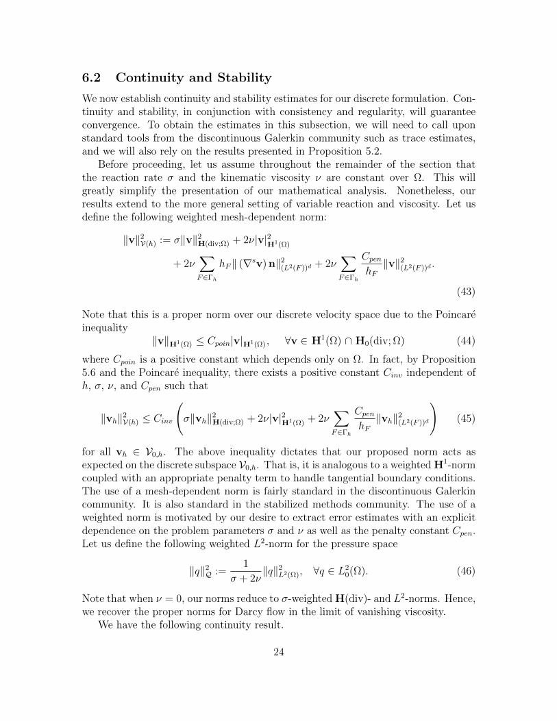
6.2 Continuity and Stability

We now establish continuity and stability estimates for our discrete formulation. Con-tinuity and stability, in conjunction with consistency and regularity, will guaranteeconvergence. To obtain the estimates in this subsection, we will need to call uponstandard tools from the discontinuous Galerkin community such as trace estimates,and we will also rely on the results presented in Proposition 5.2.

Before proceeding, let us assume throughout the remainder of the section thatthe reaction rate σ and the kinematic viscosity ν are constant over Ω. This willgreatly simplify the presentation of our mathematical analysis. Nonetheless, ourresults extend to the more general setting of variable reaction and viscosity. Let usdefine the following weighted mesh-dependent norm:

‖v‖2V(h) := σ‖v‖2

H(div;Ω) + 2ν|v|2H1(Ω)

+ 2ν∑F∈Γh

hF‖ (∇sv) n‖2(L2(F ))d + 2ν

∑F∈Γh

CpenhF‖v‖2

(L2(F ))d .

(43)

Note that this is a proper norm over our discrete velocity space due to the Poincareinequality

‖v‖H1(Ω) ≤ Cpoin|v|H1(Ω), ∀v ∈ H1(Ω) ∩ H0(div; Ω) (44)

where Cpoin is a positive constant which depends only on Ω. In fact, by Proposition5.6 and the Poincare inequality, there exists a positive constant Cinv independent ofh, σ, ν, and Cpen such that

‖vh‖2V(h) ≤ Cinv

(σ‖vh‖2

H(div;Ω) + 2ν|v|2H1(Ω) + 2ν∑F∈Γh

CpenhF‖vh‖2

(L2(F ))d

)(45)

for all vh ∈ V0,h. The above inequality dictates that our proposed norm acts asexpected on the discrete subspace V0,h. That is, it is analogous to a weighted H1-normcoupled with an appropriate penalty term to handle tangential boundary conditions.The use of a mesh-dependent norm is fairly standard in the discontinuous Galerkincommunity. It is also standard in the stabilized methods community. The use of aweighted norm is motivated by our desire to extract error estimates with an explicitdependence on the problem parameters σ and ν as well as the penalty constant Cpen.Let us define the following weighted L2-norm for the pressure space

‖q‖2Q :=

1

σ + 2ν‖q‖2

L2(Ω), ∀q ∈ L20(Ω). (46)

Note that when ν = 0, our norms reduce to σ-weighted H(div)- and L2-norms. Hence,we recover the proper norms for Darcy flow in the limit of vanishing viscosity.

We have the following continuity result.

24

Lemma 6.2. The following continuity statements hold:

ah(w,v) ≤ Ccont‖w‖V(h)‖v‖V(h), ∀w,v ∈ V0,h ⊕(

H10(Ω) ∩H3/2+ε(Ω)

)(47)

b(p,v) ≤ ‖p‖Q‖v‖V(h), ∀p ∈ L20(Ω),v ∈ V0,h ⊕

(H1

0(Ω) ∩H3/2+ε(Ω))(48)

where ε > 0 is an arbitrary positive number and Ccont is a positive constant indepen-dent of h, σ, ν, Cpen, and ε.

Proof. To establish the first estimate, we write

ah(w,v) = a(w,v)−∑F∈Γh

∫F

2ν

(((∇sv) n) ·w + ((∇sw) n) · v− Cpen

hFw · v

)

for some w,v ∈ V0,h ⊕(

H10(Ω) ∩H3/2+ε(Ω)

). We now bound ah(·, ·) term by term.

To begin, note immediately that

a(w,v) + 2ν∑F∈Γh

∫F

CpenhF

w · v ≤ ‖w‖V(h)‖v‖V(h).

Next, we write∑F∈Γh

∫F

2ν ((∇sv) n) ·w ≤ 2ν∑F∈Γh

(‖w‖(L2(F ))d‖ (∇sv) n‖(L2(F ))d

)≤ 2ν

√∑F∈Γh

hF‖ (∇sv) n‖2(L2(F ))d

√∑F∈Γh

h−1F ‖w‖2

(L2(F ))d

≤ ‖w‖V(h)‖v‖V(h).

Similarly, we have ∑F∈Γh

∫F

2ν ((∇sw) n) · v ≤ ‖w‖V(h)‖v‖V(h).

Collecting our bounds, we have

ah(w,v) ≤ Ccont‖w‖V(h)‖v‖V(h)

with Ccont = 3. To establish the second continuity result of the lemma, we first write

b(p,v) ≤ ‖p‖L2(Ω)‖divv‖L2(Ω).

25

The result is then a consequence of

‖p‖L2(Ω) = (σ + 2ν)1/2 ‖p‖Q

and‖divv‖L2(Ω) ≤ (σ + 2ν)−1/2 ‖v‖V(h).

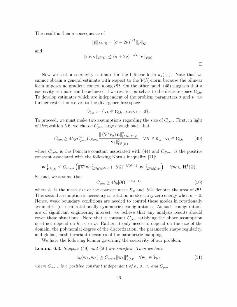
Now we seek a coercivity estimate for the bilinear form ah(·, ·). Note that wecannot obtain a general estimate with respect to the V(h)-norm because the bilinearform imposes no gradient control along ∂Ω. On the other hand, (45) suggests that acoercivity estimate can be achieved if we restrict ourselves to the discrete space V0,h.To develop estimates which are independent of the problem parameters σ and ν, wefurther restrict ourselves to the divergence-free space

V0,h := vh ∈ V0,h : divvh = 0 .

To proceed, we must make two assumptions regarding the size of Cpen. First, in lightof Proposition 5.6, we choose Cpen large enough such that

Cpen ≥ 4hKC2poinCKorn

‖ (∇svh) n‖2(L2(∂K))d

‖vh‖2H1(K)

, ∀K ∈ Kh, vh ∈ V0,h (49)

where Cpoin is the Poincare constant associated with (44) and CKorn is the positiveconstant associated with the following Korn’s inequality [11]:

|w|2H1(Ω) ≤ CKorn

(‖∇sw‖2

(L2(Ω))d×d + |∂Ω|−1/(d−1)‖w‖2(L2(∂Ω))d

), ∀w ∈ H1(Ω) .

Second, we assume thatCpen ≥ 4h0|∂Ω|−1/(d−1) (50)

where h0 is the mesh size of the coarsest mesh K0 and |∂Ω| denotes the area of ∂Ω.This second assumption is necessary as rotation modes carry zero energy when σ = 0.Hence, weak boundary conditions are needed to control these modes in rotationallysymmetric (or near rotationally symmetric) configurations. As such configurationsare of significant engineering interest, we believe that any analysis results shouldcover these situations. Note that a constant Cpen satisfying the above assumptionneed not depend on h, σ, or ν. Rather, it only needs to depend on the size of thedomain, the polynomial degree of the discretization, the parametric shape regularity,and global, mesh-invariant measures of the parametric mapping.

We have the following lemma governing the coercivity of our problem.

Lemma 6.3. Suppose (49) and (50) are satisfied. Then we have

ah(wh,wh) ≥ Ccoerc‖wh‖2V(h), ∀wh ∈ V0,h (51)

where Ccoerc is a positive constant independent of h, σ, ν, and Cpen.

26

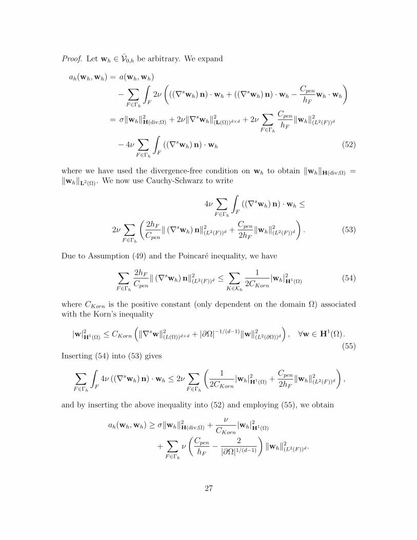
Proof. Let wh ∈ V0,h be arbitrary. We expand

ah(wh,wh) = a(wh,wh)

−∑F∈Γh

∫F

2ν

(((∇swh) n) ·wh + ((∇swh) n) ·wh −

CpenhF

wh ·wh

)= σ‖wh‖2

H(div;Ω) + 2ν‖∇swh‖2(L(Ω))d×d + 2ν

∑F∈Γh

CpenhF‖wh‖2

(L2(F ))d

− 4ν∑F∈Γh

∫F

((∇swh) n) ·wh (52)

where we have used the divergence-free condition on wh to obtain ‖wh‖H(div;Ω) =‖wh‖L2(Ω). We now use Cauchy-Schwarz to write

4ν∑F∈Γh

∫F

((∇swh) n) ·wh ≤

2ν∑F∈Γh

(2hFCpen‖ (∇swh) n‖2

(L2(F ))d +Cpen2hF‖wh‖2

(L2(F ))d

). (53)

Due to Assumption (49) and the Poincare inequality, we have∑F∈Γh

2hFCpen‖ (∇swh) n‖2

(L2(F ))d ≤∑K∈Kh

1

2CKorn|wh|2H1(Ω) (54)

where CKorn is the positive constant (only dependent on the domain Ω) associatedwith the Korn’s inequality

|w|2H1(Ω) ≤ CKorn

(‖∇sw‖2

(L(Ω))d×d + |∂Ω|−1/(d−1)‖w‖2(L2(∂Ω))d

), ∀w ∈ H1(Ω) .

(55)Inserting (54) into (53) gives∑

F∈Γh

∫F

4ν ((∇swh) n) ·wh ≤ 2ν∑F∈Γh

(1

2CKorn|wh|2H1(Ω) +

Cpen2hF‖wh‖2

(L2(F ))d

),

and by inserting the above inequality into (52) and employing (55), we obtain

ah(wh,wh) ≥ σ‖wh‖2H(div;Ω) +

ν

CKorn|wh|2H1(Ω)

+∑F∈Γh

ν

(CpenhF− 2

|∂Ω|1/(d−1)

)‖wh‖2

(L2(F ))d .

27

Invoking Assumption (50), we have

ah(wh,wh) ≥ σ‖wh‖2H(div;Ω) +

ν

CKorn|wh|2H1(Ω) +

∑F∈Γh

νCpen2hF

‖wh‖2(L2(F ))d

ashF ≤ h ≤ h0.

The lemma then follows with Ccoerc = C−1inv min

0.25, 0.5 (CKorn)−1 where Cinv is

the constant associated with (45).

We need one more stability estimate. We need to satisfy the Babuska-Brezzi inf-sup condition. Recall that we already proved an inf-sup condition for our discretespaces in Section 5. However, for that inf-sup condition, we utilized the H1-norm forthe velocity space. Here, we must employ the stronger V(h)-norm. To arrive at aninf-sup condition for this stronger norm, we will proceed by employing three pow-erful tools: (1) commuting projectors, (2) trace inequalities, and (3) approximationestimates.

Lemma 6.4. There exists a positive constant β independent of h, σ, and ν such thatthe following holds: for every qh ∈ Q0,h, there exists a vh ∈ V0,h such that:

divvh = qh (56)

and

‖vh‖V(h) ≤σ + 2ν

β‖qh‖Q. (57)

Hence,

infqh∈Q0,h,qh 6=0

supvh∈V0,h

(divvh, qh)

‖vh‖V(h)‖qh‖Q≥ β. (58)

Furthermore, the inf-sup constant β asymptotically scales inversely with the squareroot of Cpen.

Proof. Let qh ∈ Q0,h be arbitrary. Then we know there exists a function v ∈ H10(Ω)

such that divv = qh and

2ν‖v‖2H1(Ω) ≤ 2νβ−2‖qh‖2

L2(Ω)

where β is a positive constant independent of v. Let vh = Π0Vh v. Then, by Proposi-

tion 5.2, divvh = div Π0Vh v = Π0

Qhdivv = qh and

2ν‖vh‖2H1(Ω) ≤ 2νC2

u‖v‖2H1(Ω) ≤ 2νC2

uβ−2‖qh‖2

L2(Ω) (59)

28

where Cu > 0 is a positive constant independent of h, σ, η, and Cpen. Similarly, wehave

σ‖vh‖2H(div;Ω) ≤ σC2

uβ−2‖qh‖2

L2(Ω). (60)

As v satisfies homogeneous Dirichlet boundary conditions, we can apply the contin-uous trace inequality (see Theorem 3.2 of [26]) to obtain the expression∑

F∈Γh

h−1F ‖vh‖

2(L2(F ))d =

∑F∈Γh

h−1F ‖vh − v‖2

(L2(F ))d

≤ C2tr

∑K∈Kh

(h−2K ‖vh − v‖2

L2(K) + |vh − v|2H1(K)

)where Ctr is a positive constant only dependent on the shape regularity of the meshfamily Mhh≤h0 and global, mesh-invariant measures of the parametric mapping.Proposition 5.5 gives∑

K∈Kh

(h−2K ‖vh − v‖2

L2(K) + |vh − v|2H1(K)

)≤ C2

bound‖v‖2H1(Ω)

where Cbound is a positive constant independent of h, σ, ν, and Cpen. Thus, we have

2ν∑F∈Γh

CpenhF‖vh‖2

(L2(F ))d ≤ 2νC2boundC

2trCpenβ

−2‖qh‖2L2(Ω). (61)

Combining (45), (59), (60), and (61), we have

‖vh‖2V(h) ≤ Cinvβ

−2(C2u + C2

boundC2trCpen

)(σ + 2ν) ‖qh‖2

L2(Ω).

Hence, (57) holds with

β = C−1/2inv

(C2u + C2

boundC2trCpen

)−1/2β.

The inverse dependence of the inf-sup constant β on the square root of the penaltyconstant Cpen suggests that Cpen should be chosen as small as possible to satisfycoercivity. Indeed, we have numerically computed the inf-sup constant β for a widerange of values of Cpen and found that the relationship β . C

−1/2pen is sharp (for

reference, see the results listed in Table 1). We would like to note that this makesintuitive sense as we lose inf-sup stability entirely if we enforce the no-slip conditionstrongly.

By Lemmata 6.2, 6.3, and 6.4 and Brezzi’s Theorem [12], we immediately havethe following theorem establishing well-posedness.

29

Table 1: Dependence of the inf-sup constant β on Nitsche’s penalty constant Cpen fork′ = 1, h = 1/16, and Ω = (0, 1)2.

Cpen 1 2 4 8 16 32 64

β 4.24e-1 3.89e-1 3.29e-1 2.50e-1 1.82e-1 1.30e-1 9.24e-2order - -0.13 -0.24 -0.39 -0.46 -0.48 -0.49

Theorem 6.1. Suppose that the assumptions of Lemma 6.3 hold true. Then, Problem(G) has a unique weak solution (uh, ph) ∈ V0,h ×Q0,h. Furthermore,

‖uh‖V(h) ≤1

Ccoerc

(σ + 2νC−2

poin

)−1/2 ‖f‖L2(Ω), (62)

‖ph‖Q ≤1

β

(σ + 2νC−2

poin

)−1/2(

1 +CcontCcoerc

)‖f‖L2(Ω). (63)

We would like to note that all of the continuity and stability estimates here holdwhen ν is identically zero and σ is positive. Hence, we have a unified stability analysisof Stokes flow and incompressible Darcy flow.

Remark 6.2. Note that for the setting of constant viscosity, one has

∇ · (2ν∇su) = ν∆u. (64)

This inspires a different variational formulation than that presented here which isoften the basis for numerical discretization (see, for example, [19]). However, thesediscretizations (and their accompanying mathematical analysis) are not extendable tothe more difficult and physically relevant setting of variable viscosity, and they alsocannot easily accommodate traction boundary conditions.

6.3 A Priori Error Estimates

We are now ready to derive a priori error estimates for our discrete formulation. Webegin with the following lemma.

Lemma 6.5. Let (u, p) and (uh, ph) denote the unique solutions of Problems (W )and (G) respectively. Furthermore, assume that u ∈ H3/2+ε(Ω) for some ε > 0 andthat the assumptions of Lemma 6.3 hold true. Then

‖u− uh‖V(h) ≤(

1 +CcontCcoerc

)inf

vh∈V0,h‖u− vh‖V(h) (65)

and

‖p− ph‖Q ≤(

1 +1

β

)inf

qh∈Q0,h

‖p− qh‖Q +Ccont

β‖u− uh‖V(h) (66)

30

where Ccont is the continuity constants given by Lemma 6.2, Ccoerc is the coercivityconstant given by Lemma 6.3, and β is the inf-sup constant given by Lemma 6.4.

Proof. We first prove (65). We have that, for any vh ∈ V0,h such that divvh = 0,

‖vh − uh‖2V(h) ≤

1

Ccoerca(vh − uh,vh − uh)

=1

Ccoerca(vh − u,vh − uh)

≤ CcontCcoerc

‖vh − u‖V(h)‖vh − uh‖V(h) (67)

where we employed the orthogonality given by Corollary 6.1 and the condition

div (uh − vh) = 0

in the second line of the (67). Hence, we can write

‖u− uh‖V(h) ≤ infvh∈V0,h

(‖u− vh‖V(h) + ‖vh − uh‖V(h)

)≤(

1 +CcontCcoerc

)inf

vh∈V0,h‖u− vh‖V(h). (68)

We now prove (66). We have that, for any qh ∈ Q0,h,

‖ph − qh‖Q ≤1

βsup

wh∈V0,h

b(ph − qh,wh)

‖wh‖V(h)

=1

βsup

wh∈V0,h

b(p− qh,wh)− a(u− uh,wh)

‖wh‖V(h)

≤ 1

β

(‖p− qh‖Q + Ccont‖u− uh‖V(h)

)(69)

where we again employed orthogonality in the second line above. Inequality (66) thenfollows in the same manner as (68) by a splitting of the pressure error and a usage of(69).

We have the following theorem giving us a priori convergence estimates which areoptimal for the discrete velocity field and suboptimal, by one order, for the discretepressure field.

Theorem 6.2. Let (u, p) and (uh, ph) denote the unique solutions of Problems (W )and (G) respectively. Furthermore, assume that (u, p) ∈ Hj+1(Ω) ×Hj(Ω) for somej > 1/2 and that the assumptions of Lemma 6.3 hold true. Then

‖u− uh‖V(h) ≤ Cu

(1 +

CcontCcoerc

)√σh2s+2 + 2νh2s‖u‖Hs+1(Ω) (70)

31

and

‖p− ph‖Q ≤ Cp

(1 +

1

β

)(σ + 2ν)−1/2 hs‖p‖Hs(Ω) +

Ccont

β‖u− uh‖V(h) (71)

for s = min k′, j where k′ is the polynomial degree of our discretization, Cu is apositive constant independent of h, σ, and ν which asymptotically scales with thesquare root of Cpen, and Cp is a positive constant independent of h, σ, ν, and Cpen.

Proof. We first prove (70). Recall the error estimate given by (65):

‖u− uh‖V(h) ≤(

1 +CcontCcoerc

)inf

vh∈V0,h‖u− vh‖V(h).

Noting div Π0Vh u = Π0

Qhdivu = 0, we can choose vh = Π0

Vh u in the above expressionto obtain

‖u− uh‖V(h) ≤(

1 +CcontCcoerc

)‖u− Π0

Vh u‖V(h)

= Cco√T1 + T2 + T3 + T4 (72)

where we have assigned Cco =(

1 + Ccont

Ccoerc

)and

T1 = σ‖u− Π0Vh u‖2

H(div;Ω) = σ‖u− Π0Vh u‖2

L2(Ω) (73)

T2 = 2ν|u− Π0Vh u|2H1(Ω) (74)

T3 = 2ν∑F∈Γh

hF‖(∇s(u− Π0

Vh u))

n‖2(L2(F ))d (75)

T4 = 2ν∑F∈Γh

Cpenh−1F ‖u− Π0

Vh u‖2(L2(F ))d . (76)

To handle the face integral in (75), we recruit the multiplicative trace inequalityfor fractional Sobolev spaces [57] and Young’s inequality element-wise to obtain thebound ∑

F∈Γh

CpenhF‖(∇s(u− Π0

Vh u))

n‖2(L2(F ))d ≤

(Ctrc,1)2∑K∈Kh

(|u− Π0

Vh u|2H1(K) + h2qK |u− Π0

Vh u|2Hq+1(Ω)

)where 1/2 < q ≤ s and Ctrc,1 is a positive constant independent of h, σ, ν, andCpen. To handle the face integral in (76), we recruit the standard continuous trace

32

inequality element-wise to obtain the bound∑F∈Γh

Cpenh−1F ‖u− Π0

Vh u‖2(L2(F ))d ≤

(Ctrc,2)2∑K∈Kh

(h−2K ‖u− Π0

Vh u‖2L2(K) + |u− Π0

Vh u|2H1(K)

)where Ctrc,2 is a positive constant independent of h, σ, and ν which varies linearlywith the square root of Cpen. It should be noted the two constants Ctrc,1 and Ctrc,2necessarily depend on the shape regularity of the mesh family Qh≤h0 and the para-metric mapping which together give the shape regularity of the mesh family Kh≤h0 .See [26] for more details. Inserting the above two inequalities into (72) and thenapplying Proposition 5.5, we immediately acquire the bound

‖u− Π0Vh u‖V(h) ≤ CuCco

√σh2s+2 + 2νh2s‖u‖Hs+1(Ω)

for Cu a positive constant independent of h, σ, and ν with the same functionaldependency on the penalty parameter as Ctrc,2.

The proof for (71) is much more immediate. Choosing qh = Π0Qhp in the error

estimate given by (66), one obtains

‖p− ph‖Q ≤(

1 +1

β

)‖p− Π0

Qhp‖Q +

Ccont

β‖u− uh‖V(h).

Inequality (71) follows by an application of Proposition 5.5 to bound the pressureinterpolation error.

Since we have the bound

2ν| · |H1(Ω) . ‖ · ‖V(h),

the above theorem also provides optimal convergence rates for the velocity field inthe H1-norm. If we assume slightly more regularity for the pressure space, we havethe following proposition.

Proposition 6.1. Let (u, p) and (uh, ph) denote the unique solutions of Problems(W ) and (G) respectively. Furthermore, assume that (u, p) ∈ Hj+1(Ω) × Hj+1(Ω)for some j > 1/2 and that the assumptions of Lemma 6.3 hold true. Then

‖p− ph‖Q ≤ Cp,e

(1 +

1

β

)(σ + 2ν)−1/2 hs+1‖p‖Hs+1(Ω) +

Ccont

β‖u− uh‖V(h) (77)

for s = min k′, j where Cp,e is a positive constant independent of h, σ, ν, and Cpen.

33

Observe that the pressure error estimate given by the above proposition is stillsuboptimal due to the presence of the velocity error, which converges with order s forgeneral viscous flows. Let us further note that the preceding theorem and propositionare trivially extended to the setting of vanishing viscosity. In this case, the velocityerror actually converges with order s+ 1, giving optimal a priori error estimates forboth the discrete pressure field and discrete velocity field for incompressible Darcyflow.

Under an elliptic regularity assumption, we can obtain optimal estimates for thevelocity field in the L2-norm by utilizing a standard duality argument. Given theunique solutions (u, p) and (uh, ph) of Problems (W ) and (G), let us consider thefollowing ancillary problem, written in strong form.

(A)

Find (ψ, r) ∈ H10(Ω) × L2

0(Ω) such that

σψ −∇ · (2ν∇sψ) + gradr = u− uh in Ω (78)

divψ = 0 in Ω (79)

ψ = 0 on ∂Ω. (80)

The above problem has a unique weak solution (ψ, r). Before proceeding, note thatwe can formally take the divergence of (78) to obtain

∆r = 0, in Ω. (81)

Since r has zero average, it follows, at least from our formal argument, that r = 0.This argument can be made rigorous by a suitable use of convolutions and passingto the limit. Now suppose that ψ ∈ H2(Ω). We can then multiply the left and righthand sides of (78) by σψ +∇ · (2ν∇sψ) to acquire the result

‖σψ‖2L2(Ω) + ‖∇ · (2ν∇sψ) ‖2

L2(Ω) = (u− uh, σψ +∇ · (2ν∇sψ))L2(Ω) . (82)

A simple application of Cauchy-Schwarz and the triangle inequality gives

‖σψ‖2L2(Ω) + ‖∇ · (2ν∇sψ) ‖2

L2(Ω) =

‖u− uh‖L2(Ω)

(‖σψ‖L2(Ω) + ‖∇ · (2ν∇sψ) ‖L2(Ω)

)(83)

Since x2 +y2 ≥ 12(x+y)2, we can divide both sides by ‖σψ‖L2(Ω) +‖∇·(2ν∇sψ) ‖L2(Ω)

to obtain1

2

(‖σψ‖L2(Ω) + ‖∇ · (2ν∇sψ) ‖L2(Ω)

)≤ ‖u− uh‖L2(Ω). (84)

As ψ satisfies normal and tangential homogeneous Dirichlet boundary conditionsand ν is assumed positive, we can employ a combination of Korn’s inequalities andPoincare inequalities to obtain a standard elliptic regularity result of the form

‖ψ‖H2(Ω) ≤ CAν−1‖u− uh‖L2(Ω). (85)

where CA is a positive constant which only depends on the domain Ω. In view of theabove discussion, we have the following theorem.

34

Theorem 6.3. Let (u, p) and (uh, ph) denote the unique solutions of Problems (W )and (G) respectively, and let (ψ, r) denote the unique solution of Problem (A). Fur-thermore, assume that (u, p) ∈ Hj+1(Ω) ×Hj(Ω) for some j ≥ 1, that ψ ∈ H2(Ω),and that the assumptions of Lemma 6.3 hold true. Then

‖u− uh‖L2(Ω) ≤ Clhs+1‖u‖Hs+1(Ω) (86)

for s = min k′, j where Cl is a positive constant independent of h, σ, and ν whichasymptotically scales with the square root of Cpen.

Proof. Since by assumption (ψ, r) ∈ H2(Ω)×H1(Ω), consistency and symmetry give

ah(v,ψ)− b(r,v) = (u− uh,v)L2(Ω)

for all v ∈ Vh. Let us take v = u− uh. We then have

‖u− uh‖2L2(Ω) = ah(u− uh,ψ).

as div (u− uh) = 0 (or r = 0 by our preceding discussion). By using the orthogonalitygiven by Corollary 6.1, we can write

‖u− uh‖2L2(Ω) = ah(u− uh,ψ − Π0

Vhψ)

≤ Ccont‖u− uh‖V(h)‖ψ − Π0Vhψ‖V(h). (87)

We bound the interpolation error by utilizing a similar argument to that used toprove (77), obtaining

‖ψ − Π0Vhψ‖V(h) ≤ Cinterp

(σ1/2h2 + ν1/2h

)‖ψ‖H2(Ω)

for Cinterp a positive constant independent of h, σ, and ν which asymptotically scaleswith the the square root of Cpen. We can now employ the elliptic regularity condition(85) to arrive at

‖ψ − Π0Vhψ‖V(h) ≤ CACinterp

(σ1/2ν−1h2 + ν−1/2h

)‖u− uh‖L2(Ω). (88)

Inserting (88) into (87) results in

‖u− uh‖L2(Ω) ≤ CACinterpCcont(σ1/2ν−1h2 + ν−1/2h

)‖u− uh‖V(h).

Immediately invoking the error estimate given by Theorem 6.2, we obtain

‖u− uh‖L2(Ω) ≤ Ctemp

(1 +

√Dah

)2

hs+1‖u‖Hs+1(Ω) (89)

35

where Ctemp is a positive constant independent of h, σ, and ν which asymptoticallyscales with the square root of Cpen and

Dah =σh2

ν.

However, we also have the following estimate due to Theorem 6.2:

‖u− uh‖L2(Ω) ≤ Cu

(1 +

CcontCcoerc

)(1 + (Dah)

−1)1/2hs+1‖u‖Hs+1(Ω). (90)

The desired result follows by taking the minimum of (89) and (90).

This concludes our a priori error analysis. Note that, for reasonably regularexact solutions, we have obtained optimal estimates for the velocity field in boththe strong V(h)-norm as well as the weaker H1- and L2-norms. The estimates areadditionally robust with respect to the fluid coefficients σ and ν. On the otherhand, we have obtained pressure error estimates which are suboptimal by one order.This is reminiscent of error estimates for stabilized equal-order interpolations of theStokes equations and is not unexpected as both our discrete velocity and pressurespaces consist of mapped piecewise polynomials which are only complete up to degreek′. However, our later numerical studies suggest the conservative nature of theseestimates by revealing, for simple model problems, optimal convergence rates for thepressure field. Ongoing work is being dedicated to the theoretical confirmation ofthese convergence rates. Note that our analysis covers typical singular solutions ofthe generalized Stokes equations. Later in this chapter, we will numerically study theeffectiveness of our method for a selection of singular Stokes problems. Finally, wewould like to mention that our velocity error estimates are completely independentof the pressure field. This property does not hold for discretizations which preservethe incompressibility in only a discrete sense.

Remark 6.3. In opposition to standard Bubnov-Galerkin methods, the constant(1 + Ccont (Ccoerc)

−1)appearing in (65) cannot be reduced to just Ccont (Ccoerc)

−1.

Remark 6.4. At this point, suitable requirements guaranteeing elliptic regularity fordomains obtained by NURBS mappings are unknown. One anticipates that such re-quirements should be less stringent than those associated with polyhedral domains(namely, convexity) because of enhanced smoothness. In our view, this is an interest-ing area of research.

36

F1

F2

F3

!3

!1

!2

"1

"2

x1

x2

1

1

0

0

Figure 8: Example multi-patch construction in R2.

7 Extension to Multi-Patch Domains

As was mentioned previously in Subsection 4.3, most geometries of scientific andengineering interest cannot be represented by a single patch. Instead, the multi-patch concept must be invoked. We assume that there exist np sufficiently smoothparametric mappings Fi : (0, 1)d → Rd such that the subdomains

Ωi = Fi

(Ω), i = 1, . . . , np

are non-overlapping andΩ = ∪np

i=1Ωi.

We refer to each subdomain Ωi (and its pre-image) as a patch. For a visual depictionof a multi-patch construction in R2, see Figure 8. We build discrete velocity andpressure spaces over each patch Ωi, i = 1, . . . , np in the same manner as in theprevious sections except that we do not yet enforce boundary conditions, and wedenote these spaces as Vh(Ωi) and Qh(Ωi).

To proceed further, we must make some assumptions. First of all, we assume thatif two disjoint patches Ωi and Ωj have the property that ∂Ωi ∩ ∂Ωj 6= ∅, then thisintersection consists strictly of patch faces, edges, and corners. More succinctly, twopatches cannot intersect along an isolated portion of a face (or edge) interior. Second,

37

we assume that the mappings Finp

i=1 are compatible in the following sense: if twopatches Ωi and Ωj share a face, then Fi and Fj parametrize that face identically upto changes in orientation. Third, we assume that if two patches Ωi and Ωj share aface, the B-spline meshes associated with the patches are identical along that face.This guarantees our mesh is conforming. Finally, we assume for simplicity that k1 =. . . = kd = k∗ for all patches. The mixed polynomial degree case introduces additionalcomplications that are beyond the scope of this work. We would like to note that allfour assumptions hold if we employ a conforming NURBS multi-patch construction.See, for example, Chapter 2 of [20].

We define our global discrete velocity and pressure spaces as follows:

V0,h := vh ∈ H0 (div; Ω) : vh|Ωi∈ Vh(Ωi), ∀i = 1, . . . , np , (91)

Q0,h :=qh ∈ L2

0 (Ω) : qh|Ωi∈ Qh(Ωi), ∀i = 1, . . . , np

. (92)

The space V0,h is easily constructed due to our preceding four assumptions and useof open knot vectors. Specifically, we set to zero the coefficient of any basis functionwhose normal is nonzero along ∂Ω, and along shared faces between patches, we (i)equivalence the coefficients of any basis functions whose normal values are nonzeroand equal in magnitude and direction and (ii) set opposite the coefficients of anybasis functions whose normal values are nonzero, equal in magnitude, and oppositein direction. We note that this is precisely the same procedure as is used to constructRaviart-Thomas spaces on conforming finite element meshes. We simply have patchesinstead of elements. It is easily shown that the spaces V0,h and Q0,h, along with thedivergence operator, form the bounded discrete cochain complex

V0,hdiv−−−→ Q0,h.

However, functions in V0,h do not necessarily lie in H1(Ω) as tangential continuity isnot enforced across patch interfaces. Hence, we need to account for this lack of conti-nuity when designing a discretization scheme for the generalized Stokes equations. Weemploy the symmetric interior penalty method [1, 24, 62], a standard technique in thediscontinuous Galerkin community, to weakly enforce tangential continuity betweenadjacent patches.

We now establish some preliminary notation. Let Kh(Ωi) and Fh(Ωi) denote thesets of physical mesh elements and faces associated with patch Ωi. We denote theglobal set of mesh elements as Kh and the global set of mesh faces as Fh. As in thesingle patch setting, we define the boundary mesh to be

Γh = F ∈ Fh(Ωi), i = 1, . . . , np : F ⊂ ∂Ω , (93)

and we define the interface mesh to be

Ih = F ∈ Fh(Ωi), i = 1, . . . , np : F ∈ Fh(Ωj), i 6= j and F /∈ Γh . (94)

38

For each face F ∈ Ih belonging to the interface mesh, there exist two unique adjacentelements K+, K− ∈ Kh such that F ∈ ∂K+ and F ∈ ∂K−. We define for such a facethe mesh size

hF :=1

2(hK+ + hK−) . (95)

Let φ be an arbitrary scalar-, vector-, or matrix-valued piecewise smooth function,and let us denote by φ+ and φ− the traces of φ on F as taken from within the interiorof K+ and K− respectively. We define the mean value of φ at x ∈ F as

φ :=1

2

(φ+ + φ−

). (96)

Further, for a generic multiplication operator , we define the jump of φn at x ∈ Fas

Jφ nK := φ+ nK+ + φ− nK− (97)

where nK+/− denotes the outward facing normal on the boundary ∂K+/− of elementK+/−.

With the above notation established, let us define the following bilinear form:

a∗h(w,v) =

np∑i=1

((2ν∇sw,∇sv)(L2(Ωi))d×d + (σw,v)L2(Ωi

))

−∑F∈Ih

∫F

2ν (∇sv : Jw⊗ nK + ∇sw : Jv⊗ nK) ds

+∑F∈Ih

∫F

2ν

(2CpenhF

Jw⊗ nK : Jv⊗ nK)ds

−∑F∈Γh

∫F

2ν

(((∇sv) n) ·w + ((∇sw) n) · v− Cpen

hFw · v

)ds. (98)

Above, Cpen > 0 denotes the same positive penalty constant as before. Our discreteformulation over the multi-patch domain then reads as follows.

(MP )

Find uh ∈ V0,h and ph ∈ Q0,h such that

a∗h(uh,vh)− b(ph,vh) + b(qh,uh) = (f,vh)L2(Ω) (99)

for all vh ∈ V0,h and qh ∈ Q0,h.

As in the single patch setting, the discrete formulation detailed above returns a point-wise divergence-free velocity field. However, we do not have a convergence analysisavailable as we do not yet have a multi-patch analogue of Proposition 5.2. We antic-ipate this will take new theoretical developments. Nonetheless, we have utilized theabove formulation in practice and observed it returns optimal convergence rates forboth velocity and pressure fields.

39

8 Numerical Verification of Convergence Estimates

In this section, we numerically verify our convergence estimates using a collection ofproblems with exact solutions. Throughout, we choose Nitsche’s penalty constant as

Cpen = 5(k′ + 1)

where k′ is the polynomial degree of a given discretization. We have found that thischoice leads to stable numerical formulations for the generalized Stokes equations.Furthermore, unless otherwise specified, we employ uniform parametric meshes, linearparametric mappings, and B-spline spaces of maximal continuity.

8.1 Two-Dimensional Manufactured Solution

As a first numerical experiment, we consider a two-dimensional manufactured solutionthat was originally presented in [14]. Let

Ω ≡ (0, 1)2

andf ≡ σu−∇ · (2ν∇su) +∇p

with

u =

[2ex(−1 + x)2x2(y2 − y)(−1 + 2y)

(−ex(−1 + x)x(−2 + x(3 + x))(−1 + y)2y2)

]and

p = (−424 + 156e+ (y2 − y)(−456 + ex(456 + x2(228− 5(y2 − y))+2x(−228 + (y2 − y)) + 2x3(−36 + (y2 − y)) + x4(12 + (y2 − y))))).

Homogeneous boundary conditions are applied along the boundary ∂Ω, and the pres-sure is enforced to satisfy

∫Ωpdx = 0. The unique solution to the generalized Stokes

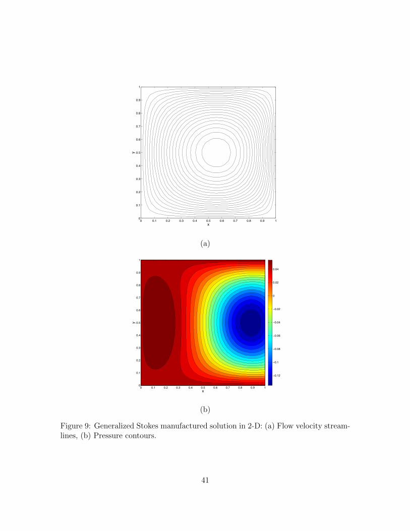
equation with the prescribed forcing is then clearly (u, p) = (u, p). The streamlinesand pressure contours associated with the exact solution are plotted in Figure 9. Notefrom the streamline plot that the velocity solution has a simple vortex structure.

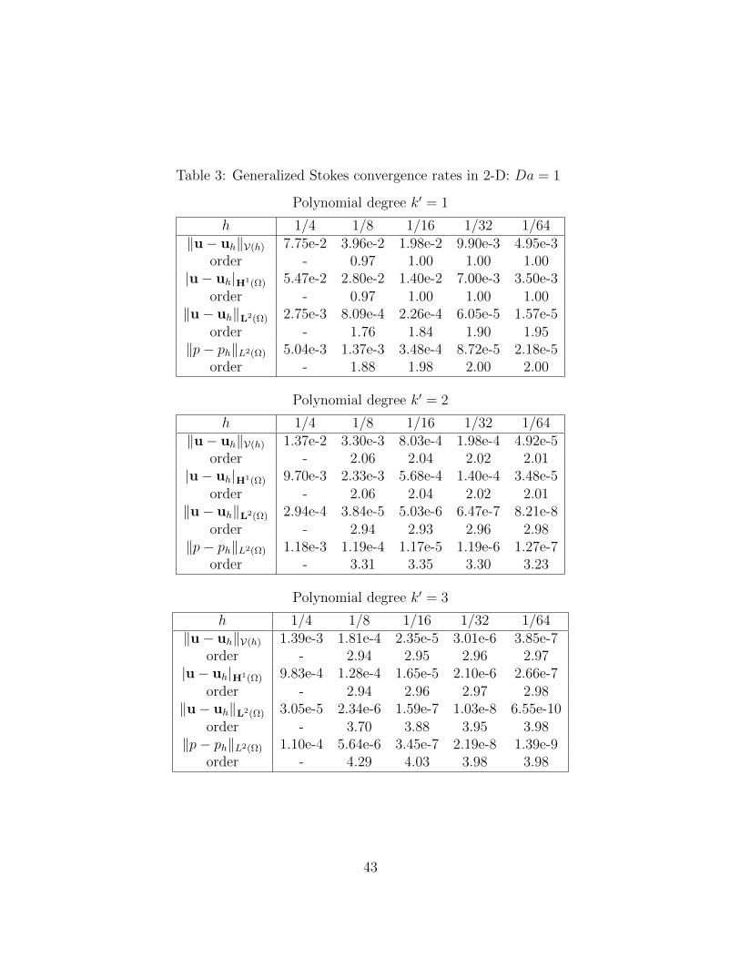
For the above constructed solution, we have computed convergence rates fordivergence-conforming B-spline discretizations of varying mesh size and polynomialdegree. Furthermore, we have computed convergence rates for a variety of Damkohlernumbers

Da =σL2

ν

where L is a length parameter which we henceforth specify as one. These convergencerates are provided in Tables 2, 3, and 4. Note immediately from the tables that ourtheoretically derived error estimates are confirmed. Second, note that the L2-normof the pressure error optimally converges like O(hk

′+1), which is an improvement

40

x

y

0 0.1 0.2 0.3 0.4 0.5 0.6 0.7 0.8 0.9 10

0.1

0.2

0.3

0.4

0.5

0.6

0.7

0.8

0.9

1

(a)

x

y

0 0.1 0.2 0.3 0.4 0.5 0.6 0.7 0.8 0.9 10

0.1

0.2

0.3

0.4

0.5

0.6

0.7

0.8

0.9

1

−0.12

−0.1

−0.08

−0.06

−0.04

−0.02

0

0.02

0.04

(b)

Figure 9: Generalized Stokes manufactured solution in 2-D: (a) Flow velocity stream-lines, (b) Pressure contours.

41

Table 2: Generalized Stokes convergence rates in 2-D: Da = 0

Polynomial degree k′ = 1

h 1/4 1/8 1/16 1/32 1/64‖u− uh‖V(h) 7.75e-2 3.96e-2 1.98e-2 9.90e-3 4.95e-3

order - 0.97 1.00 1.00 1.00|u− uh|H1(Ω) 5.48e-2 2.80e-2 1.40e-2 7.00e-3 3.50e-3

order - 0.97 1.00 1.00 1.00‖u− uh‖L2(Ω) 2.77e-3 8.16e-4 2.28e-4 6.10e-5 1.58e-5

order - 1.76 1.84 1.90 1.95‖p− ph‖L2(Ω) 5.04e-3 1.38e-3 3.49e-4 8.72e-5 2.18e-5

order - 1.87 1.98 2.00 2.00

Polynomial degree k′ = 2

h 1/4 1/8 1/16 1/32 1/64‖u− uh‖V(h) 1.37e-2 3.30e-3 8.03e-4 1.98e-4 4.92e-5

order - 2.06 2.04 2.02 2.01|u− uh|H1(Ω) 9.70e-3 2.33e-3 5.68e-4 1.40e-4 3.48e-5

order - 2.06 2.04 2.02 2.01‖u− uh‖L2(Ω) 2.94e-4 3.84e-5 5.03e-6 6.47e-7 8.21e-8

order - 2.94 2.93 2.96 2.98‖p− ph‖L2(Ω) 1.18e-3 1.19e-4 1.17e-5 1.19e-6 1.27e-7

order - 3.31 3.35 3.30 3.23

Polynomial degree k′ = 3

h 1/4 1/8 1/16 1/32 1/64‖u− uh‖V(h) 1.39e-3 1.81e-4 2.33e-5 3.01e-6 3.85e-7

order - 2.94 2.96 2.95 2.97|u− uh|H1(Ω) 9.83e-4 1.28e-4 1.65e-5 2.10e-6 2.66e-7

order - 2.94 2.96 2.97 2.98‖u− uh‖L2(Ω) 3.05e-5 2.34e-6 1.59e-7 1.03e-8 6.55e-10

order - 3.70 3.88 3.95 3.98‖p− ph‖L2(Ω) 1.10e-4 5.64e-6 3.45e-7 2.19e-8 1.39e-9

order - 4.29 4.03 3.98 3.98

42

Table 3: Generalized Stokes convergence rates in 2-D: Da = 1

Polynomial degree k′ = 1

h 1/4 1/8 1/16 1/32 1/64‖u− uh‖V(h) 7.75e-2 3.96e-2 1.98e-2 9.90e-3 4.95e-3

order - 0.97 1.00 1.00 1.00|u− uh|H1(Ω) 5.47e-2 2.80e-2 1.40e-2 7.00e-3 3.50e-3

order - 0.97 1.00 1.00 1.00‖u− uh‖L2(Ω) 2.75e-3 8.09e-4 2.26e-4 6.05e-5 1.57e-5

order - 1.76 1.84 1.90 1.95‖p− ph‖L2(Ω) 5.04e-3 1.37e-3 3.48e-4 8.72e-5 2.18e-5

order - 1.88 1.98 2.00 2.00

Polynomial degree k′ = 2

h 1/4 1/8 1/16 1/32 1/64‖u− uh‖V(h) 1.37e-2 3.30e-3 8.03e-4 1.98e-4 4.92e-5

order - 2.06 2.04 2.02 2.01|u− uh|H1(Ω) 9.70e-3 2.33e-3 5.68e-4 1.40e-4 3.48e-5

order - 2.06 2.04 2.02 2.01‖u− uh‖L2(Ω) 2.94e-4 3.84e-5 5.03e-6 6.47e-7 8.21e-8

order - 2.94 2.93 2.96 2.98‖p− ph‖L2(Ω) 1.18e-3 1.19e-4 1.17e-5 1.19e-6 1.27e-7

order - 3.31 3.35 3.30 3.23

Polynomial degree k′ = 3

h 1/4 1/8 1/16 1/32 1/64‖u− uh‖V(h) 1.39e-3 1.81e-4 2.35e-5 3.01e-6 3.85e-7

order - 2.94 2.95 2.96 2.97|u− uh|H1(Ω) 9.83e-4 1.28e-4 1.65e-5 2.10e-6 2.66e-7

order - 2.94 2.96 2.97 2.98‖u− uh‖L2(Ω) 3.05e-5 2.34e-6 1.59e-7 1.03e-8 6.55e-10

order - 3.70 3.88 3.95 3.98‖p− ph‖L2(Ω) 1.10e-4 5.64e-6 3.45e-7 2.19e-8 1.39e-9

order - 4.29 4.03 3.98 3.98

43

Table 4: Generalized Stokes convergence rates in 2-D: Da = 1000

Polynomial degree k′ = 1

h 1/4 1/8 1/16 1/32 1/64‖u− uh‖V(h) 3.13e-3 1.33e-3 6.36e-4 3.14e-4 1.57e-4

order - 1.23 1.06 1.02 1.00|u− uh|H1(Ω) 5.50e-2 2.78e-2 1.39e-2 6.98e-3 3.49-3

order - 0.98 1.00 0.99 1.00‖u− uh‖L2(Ω) 1.93e-3 4.79e-4 1.22e-4 3.20e-5 8.38e-6

order - 2.01 1.97 1.93 1.93‖p− ph‖L2(Ω) 3.37e-3 7.97e-4 1.96e-4 4.89e-5 1.22e-5

order - 2.08 2.02 2.00 2.00

Polynomial degree k′ = 2

h 1/4 1/8 1/16 1/32 1/64‖u− uh‖V(h) 5.24e-4 1.11e-4 2.58e-5 6.30e-6 1.55e-6

order - 2.24 2.11 2.03 2.02|u− uh|H1(Ω) 9.85e-3 2.32e-3 5.67e-4 1.40e-4 3.48e-5

order - 2.08 2.03 2.02 2.01‖u− uh‖L2(Ω) 2.83e-4 3.80e-5 5.01e-6 6.46e-7 8.21e-8

order - 2.90 2.92 2.96 2.98‖p− ph‖L2(Ω) 4.69e-4 5.36e-5 6.42e-6 7.97e-7 9.98e-8

order - 3.13 3.06 3.01 3.00

Polynomial degree k′ = 3

h 1/4 1/8 1/16 1/32 1/64‖u− uh‖V(h) 5.31e-5 6.12e-6 7.57e-7 9.56e-8 1.22e-8

order - 3.12 3.02 2.99 2.97|u− uh|H1(Ω) 9.74e-4 1.26e-4 1.64e-5 2.10e-6 2.66e-7

order - 2.95 2.94 2.97 2.98‖u− uh‖L2(Ω) 3.04e-5 2.33e-6 1.59e-7 1.03e-8 6.55e-10

order - 3.71 3.89 3.95 3.98‖p− ph‖L2(Ω) 7.56e-5 4.60e-6 3.19e-7 2.12e-8 1.37e-9

order - 4.04 3.89 3.91 3.95

44

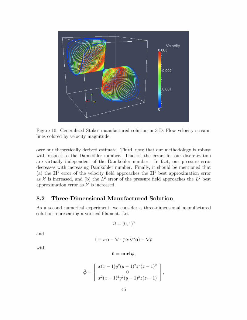
Figure 10: Generalized Stokes manufactured solution in 3-D: Flow velocity stream-lines colored by velocity magnitude.

over our theoretically derived estimate. Third, note that our methodology is robustwith respect to the Damkohler number. That is, the errors for our discretizationare virtually independent of the Damkohler number. In fact, our pressure errordecreases with increasing Damkohler number. Finally, it should be mentioned that(a) the H1 error of the velocity field approaches the H1 best approximation erroras k′ is increased, and (b) the L2 error of the pressure field approaches the L2 bestapproximation error as k′ is increased.

8.2 Three-Dimensional Manufactured Solution

As a second numerical experiment, we consider a three-dimensional manufacturedsolution representing a vortical filament. Let

Ω ≡ (0, 1)3

andf ≡ σu−∇ · (2ν∇su) +∇p

withu = curlφ,

φ =

x(x− 1)y2(y − 1)2z2(z − 1)2

0x2(x− 1)2y2(y − 1)2z(z − 1)

,45

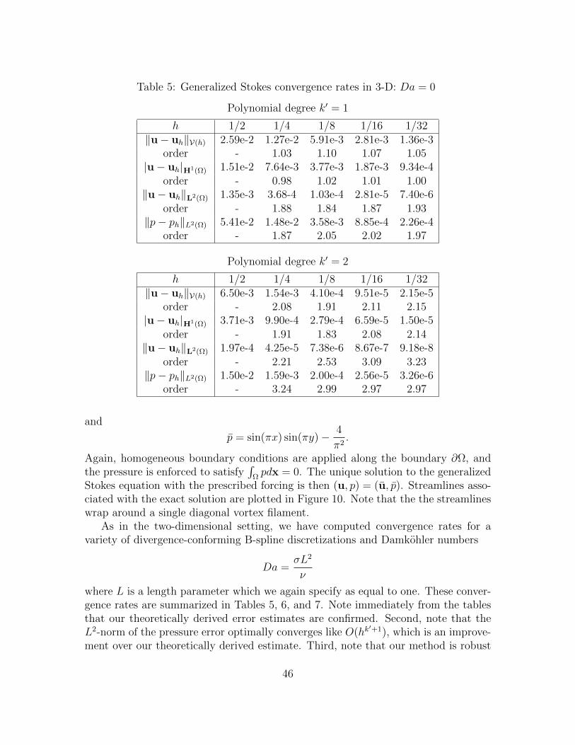
Table 5: Generalized Stokes convergence rates in 3-D: Da = 0

Polynomial degree k′ = 1

h 1/2 1/4 1/8 1/16 1/32‖u− uh‖V(h) 2.59e-2 1.27e-2 5.91e-3 2.81e-3 1.36e-3

order - 1.03 1.10 1.07 1.05|u− uh|H1(Ω) 1.51e-2 7.64e-3 3.77e-3 1.87e-3 9.34e-4

order - 0.98 1.02 1.01 1.00‖u− uh‖L2(Ω) 1.35e-3 3.68-4 1.03e-4 2.81e-5 7.40e-6

order - 1.88 1.84 1.87 1.93‖p− ph‖L2(Ω) 5.41e-2 1.48e-2 3.58e-3 8.85e-4 2.26e-4

order - 1.87 2.05 2.02 1.97

Polynomial degree k′ = 2

h 1/2 1/4 1/8 1/16 1/32‖u− uh‖V(h) 6.50e-3 1.54e-3 4.10e-4 9.51e-5 2.15e-5

order - 2.08 1.91 2.11 2.15|u− uh|H1(Ω) 3.71e-3 9.90e-4 2.79e-4 6.59e-5 1.50e-5

order - 1.91 1.83 2.08 2.14‖u− uh‖L2(Ω) 1.97e-4 4.25e-5 7.38e-6 8.67e-7 9.18e-8

order - 2.21 2.53 3.09 3.23‖p− ph‖L2(Ω) 1.50e-2 1.59e-3 2.00e-4 2.56e-5 3.26e-6

order - 3.24 2.99 2.97 2.97

and

p = sin(πx) sin(πy)− 4

π2.

Again, homogeneous boundary conditions are applied along the boundary ∂Ω, andthe pressure is enforced to satisfy

∫Ωpdx = 0. The unique solution to the generalized

Stokes equation with the prescribed forcing is then (u, p) = (u, p). Streamlines asso-ciated with the exact solution are plotted in Figure 10. Note that the the streamlineswrap around a single diagonal vortex filament.

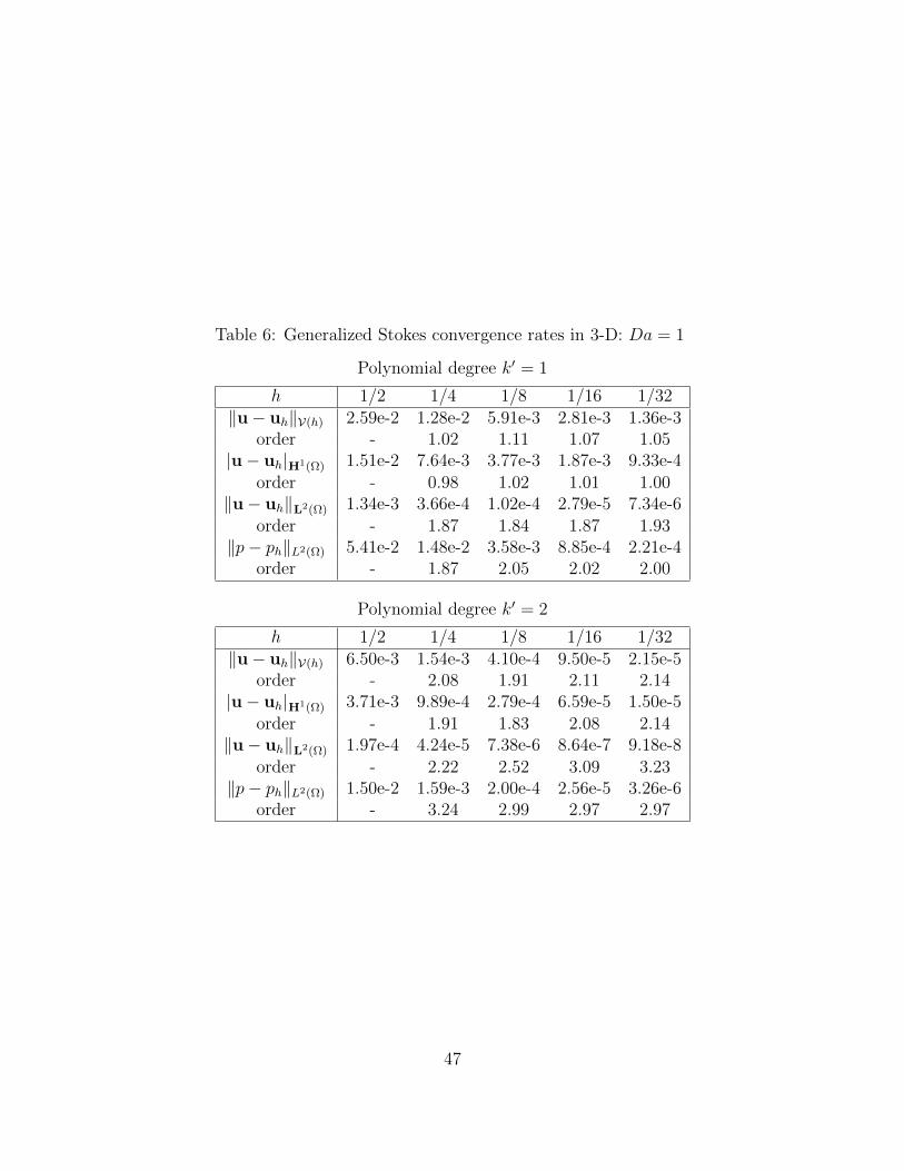
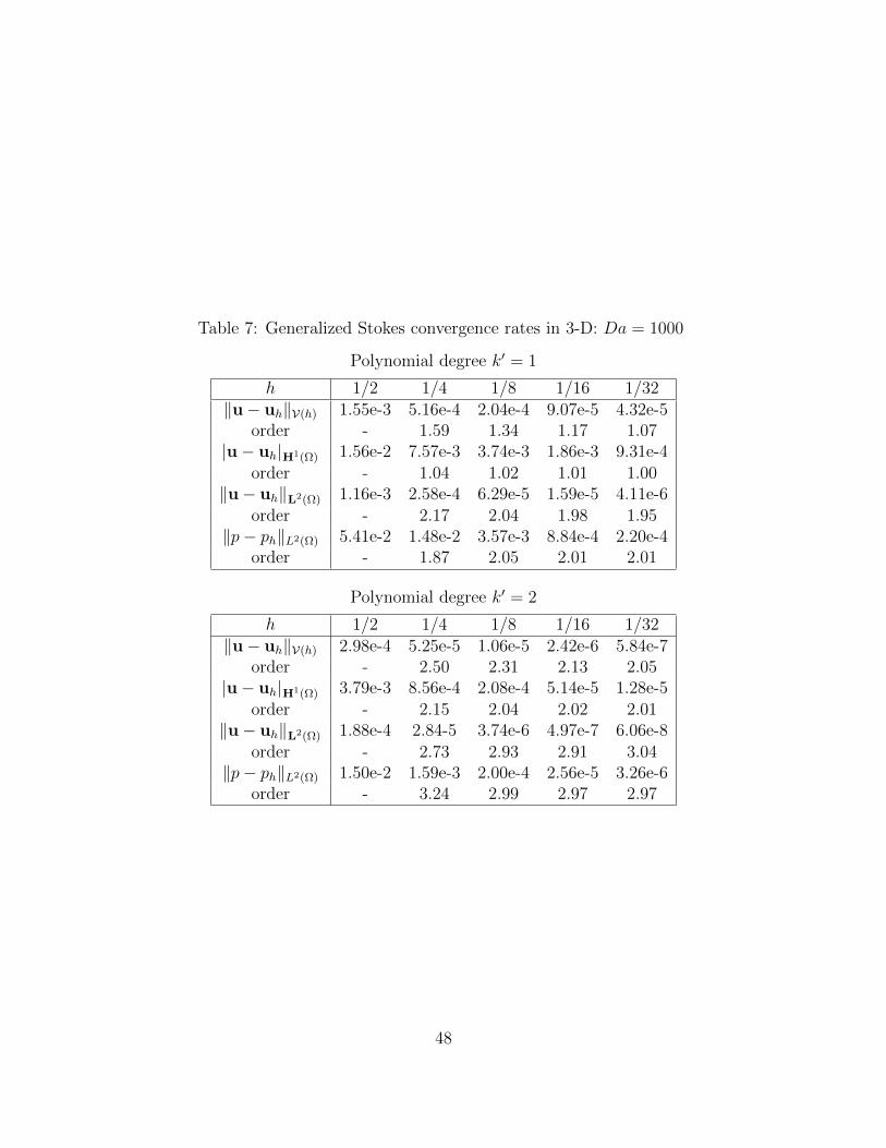
As in the two-dimensional setting, we have computed convergence rates for avariety of divergence-conforming B-spline discretizations and Damkohler numbers

Da =σL2

ν

where L is a length parameter which we again specify as equal to one. These conver-gence rates are summarized in Tables 5, 6, and 7. Note immediately from the tablesthat our theoretically derived error estimates are confirmed. Second, note that theL2-norm of the pressure error optimally converges like O(hk

′+1), which is an improve-ment over our theoretically derived estimate. Third, note that our method is robust

46

Table 6: Generalized Stokes convergence rates in 3-D: Da = 1

Polynomial degree k′ = 1

h 1/2 1/4 1/8 1/16 1/32‖u− uh‖V(h) 2.59e-2 1.28e-2 5.91e-3 2.81e-3 1.36e-3

order - 1.02 1.11 1.07 1.05|u− uh|H1(Ω) 1.51e-2 7.64e-3 3.77e-3 1.87e-3 9.33e-4

order - 0.98 1.02 1.01 1.00‖u− uh‖L2(Ω) 1.34e-3 3.66e-4 1.02e-4 2.79e-5 7.34e-6

order - 1.87 1.84 1.87 1.93‖p− ph‖L2(Ω) 5.41e-2 1.48e-2 3.58e-3 8.85e-4 2.21e-4

order - 1.87 2.05 2.02 2.00

Polynomial degree k′ = 2

h 1/2 1/4 1/8 1/16 1/32‖u− uh‖V(h) 6.50e-3 1.54e-3 4.10e-4 9.50e-5 2.15e-5

order - 2.08 1.91 2.11 2.14|u− uh|H1(Ω) 3.71e-3 9.89e-4 2.79e-4 6.59e-5 1.50e-5

order - 1.91 1.83 2.08 2.14‖u− uh‖L2(Ω) 1.97e-4 4.24e-5 7.38e-6 8.64e-7 9.18e-8

order - 2.22 2.52 3.09 3.23‖p− ph‖L2(Ω) 1.50e-2 1.59e-3 2.00e-4 2.56e-5 3.26e-6

order - 3.24 2.99 2.97 2.97

47

Table 7: Generalized Stokes convergence rates in 3-D: Da = 1000

Polynomial degree k′ = 1

h 1/2 1/4 1/8 1/16 1/32‖u− uh‖V(h) 1.55e-3 5.16e-4 2.04e-4 9.07e-5 4.32e-5

order - 1.59 1.34 1.17 1.07|u− uh|H1(Ω) 1.56e-2 7.57e-3 3.74e-3 1.86e-3 9.31e-4

order - 1.04 1.02 1.01 1.00‖u− uh‖L2(Ω) 1.16e-3 2.58e-4 6.29e-5 1.59e-5 4.11e-6

order - 2.17 2.04 1.98 1.95‖p− ph‖L2(Ω) 5.41e-2 1.48e-2 3.57e-3 8.84e-4 2.20e-4

order - 1.87 2.05 2.01 2.01

Polynomial degree k′ = 2

h 1/2 1/4 1/8 1/16 1/32‖u− uh‖V(h) 2.98e-4 5.25e-5 1.06e-5 2.42e-6 5.84e-7

order - 2.50 2.31 2.13 2.05|u− uh|H1(Ω) 3.79e-3 8.56e-4 2.08e-4 5.14e-5 1.28e-5

order - 2.15 2.04 2.02 2.01‖u− uh‖L2(Ω) 1.88e-4 2.84-5 3.74e-6 4.97e-7 6.06e-8

order - 2.73 2.93 2.91 3.04‖p− ph‖L2(Ω) 1.50e-2 1.59e-3 2.00e-4 2.56e-5 3.26e-6

order - 3.24 2.99 2.97 2.97

48

with respect to the Damkohler number. Finally, let us remark the exact velocity fieldis recovered for discretizations of degree k′ ≥ 3.

8.3 Two-Dimensional Problem with a Singular Solution

To examine how our discretization performs in the presence of singularities, we con-sider Stokes flow in the L-shaped domain Ω = (−1, 1)2)\([0, 1) × (−1, 0]). The flowproblem in consideration is depicted in Figure 11(a). Homogeneous Dirichlet bound-ary conditions are applied along ΓD = (0, y) : y ∈ (−1, 0) ∪ (x, 0) : x ∈ (0, 1),Neumann boundary conditions are applied along ΓN = ∂Ω\ΓD, and we set σ = 0,ν = 1, and f = 0. As in [60], the Neumann boundary conditions are chosen such thatthe exact solution is

u =

[rλ((1 + λ) sin(θ)ψ(θ) + cos(θ)ψ′(θ)rλ(−(1 + λ) cos(θ)ψ(θ) + sin(θ)ψ′(θ)

]and

p = −rλ−1 ((1 + λ)2φ′(θ) + φ′′′(θ)) /(1− λ)

where (r, θ) are polar coordinates with respect to the origin (0, 0),

φ = sin((1 + λ)θ) cos(λω)/(1 + λ)− cos((1 + λ)θ)− sin((1− λ)θ) cos(λω)/(1− λ) + cos((1− λ)θ),

ω = 32φ, and λ ≈ 0.54448373678246 is the smallest positive root of

sin(λω) + λ sin(ω) = 0.

This singular solution is illustrated in Figure 12. Note that (u, p) ∈ H1+λ(Ω) ×Hλ(Ω). This is the strongest corner singularity for the Stokes operator in the L-shaped domain, and, as such, this numerical example models typical singular behaviorobserved in the vicinity of reentrant corners.

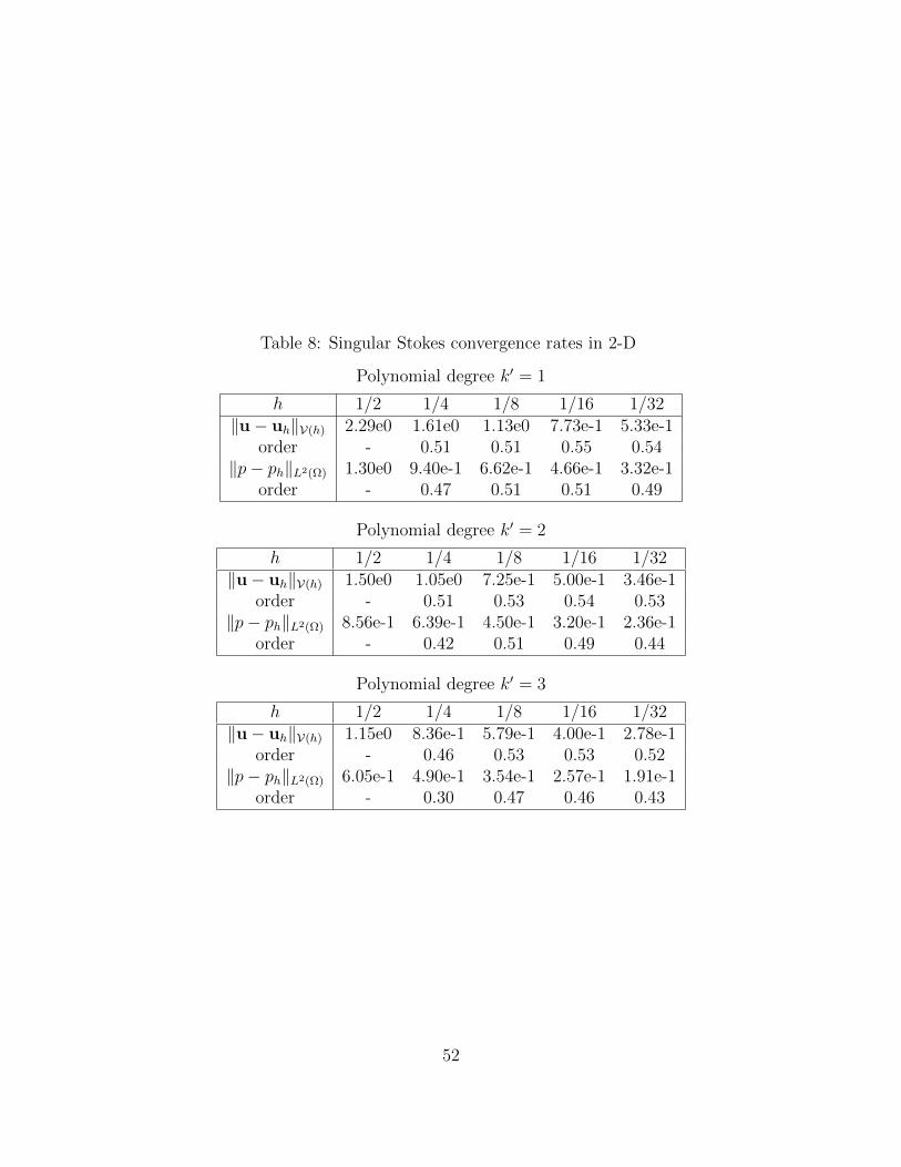
To compute this flow example using our discretization technique, we must resortto a multi-patch construction. We utilize the three-patch construction illustrated inFigure 11(b). Each patch is mapped from the parametric domain using an affineparametrization. As discussed in Section 7, we impose normal continuity strongly be-tween patches and tangential continuity weakly using the symmetric interior penaltymethod. We have computed convergence rates for a variety of divergence-conformingB-spline discretizations and reported our results in Table 8. Note from the table thatthe V(h)-norm of the velocity field and the L2-norm of the pressure field are approach-ing the optimal convergence rates of O(hλ) as h→ 0. Furthermore, note the velocityand pressure errors improve with increasing polynomial degree. This is somewhatcounterintuitive as we also increase smoothness with polynomial degree. This beingsaid, such a property has also been observed in the context of Maxwell’s equations[15]. While we only employed uniform meshes for the computations reported here,one could of course obtain more satisfactory results with geometrically graded meshes[30, 31].

49

No-slip Walls

Traction

BC

(a)

Patch 1

Patch 2 Patch 3

(b)

Figure 11: Singular Stokes solution in 2-D: (a) Problem setup, (b) Multi-patch con-struction.

50

x

y

−1 −0.8 −0.6 −0.4 −0.2 0 0.2 0.4 0.6 0.8 1

−1

−0.8

−0.6

−0.4

−0.2

0

0.2

0.4

0.6

0.8

1

(a)

x

y

−1 −0.8 −0.6 −0.4 −0.2 0 0.2 0.4 0.6 0.8 1

−1

−0.8

−0.6

−0.4

−0.2

0

0.2

0.4

0.6

0.8

1

−50

−40

−30

−20

−10

0

10

20

30

40

50

(b)

Figure 12: Singular Stokes solution in 2-D: (a) Flow velocity streamlines, (b) Pressurecontours.

51

Table 8: Singular Stokes convergence rates in 2-D

Polynomial degree k′ = 1

h 1/2 1/4 1/8 1/16 1/32‖u− uh‖V(h) 2.29e0 1.61e0 1.13e0 7.73e-1 5.33e-1

order - 0.51 0.51 0.55 0.54‖p− ph‖L2(Ω) 1.30e0 9.40e-1 6.62e-1 4.66e-1 3.32e-1

order - 0.47 0.51 0.51 0.49

Polynomial degree k′ = 2

h 1/2 1/4 1/8 1/16 1/32‖u− uh‖V(h) 1.50e0 1.05e0 7.25e-1 5.00e-1 3.46e-1

order - 0.51 0.53 0.54 0.53‖p− ph‖L2(Ω) 8.56e-1 6.39e-1 4.50e-1 3.20e-1 2.36e-1

order - 0.42 0.51 0.49 0.44

Polynomial degree k′ = 3

h 1/2 1/4 1/8 1/16 1/32‖u− uh‖V(h) 1.15e0 8.36e-1 5.79e-1 4.00e-1 2.78e-1

order - 0.46 0.53 0.53 0.52‖p− ph‖L2(Ω) 6.05e-1 4.90e-1 3.54e-1 2.57e-1 1.91e-1

order - 0.30 0.47 0.46 0.43

52

8.4 Cylindrical Couette Flow

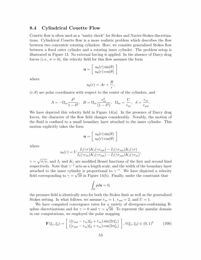
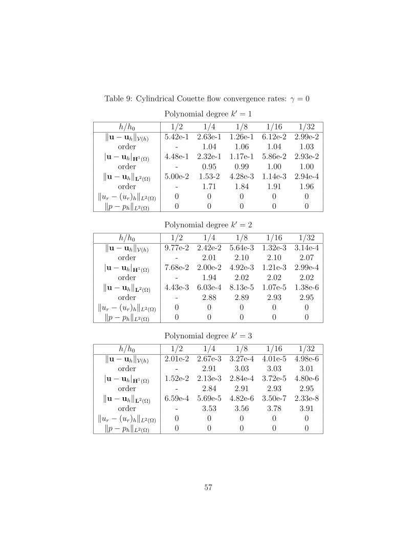
Couette flow is often used as a “sanity check” for Stokes and Navier-Stokes discretiza-tions. Cylindrical Couette flow is a more realistic problem which describes the flowbetween two concentric rotating cylinders. Here, we consider generalized Stokes flowbetween a fixed outer cylinder and a rotating inner cylinder. The problem setup isillustrated in Figure 13. No external forcing is applied. In the absence of Darcy dragforces (i.e., σ = 0), the velocity field for this flow assumes the form

u =

[uθ(r) sin(θ)uθ(r) cos(θ)

]where

uθ(r) = Ar +B

r,

(r, θ) are polar coordinates with respect to the center of the cylinders, and

A = −Ωinδ2

1− δ2, B = Ωin

r2in

(1− δ2), Ωin =

U

rin, δ =

rinrout

.

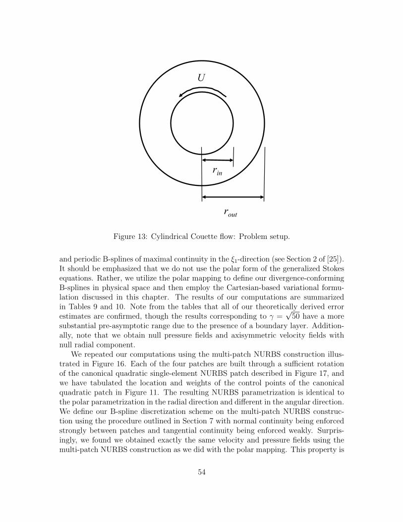
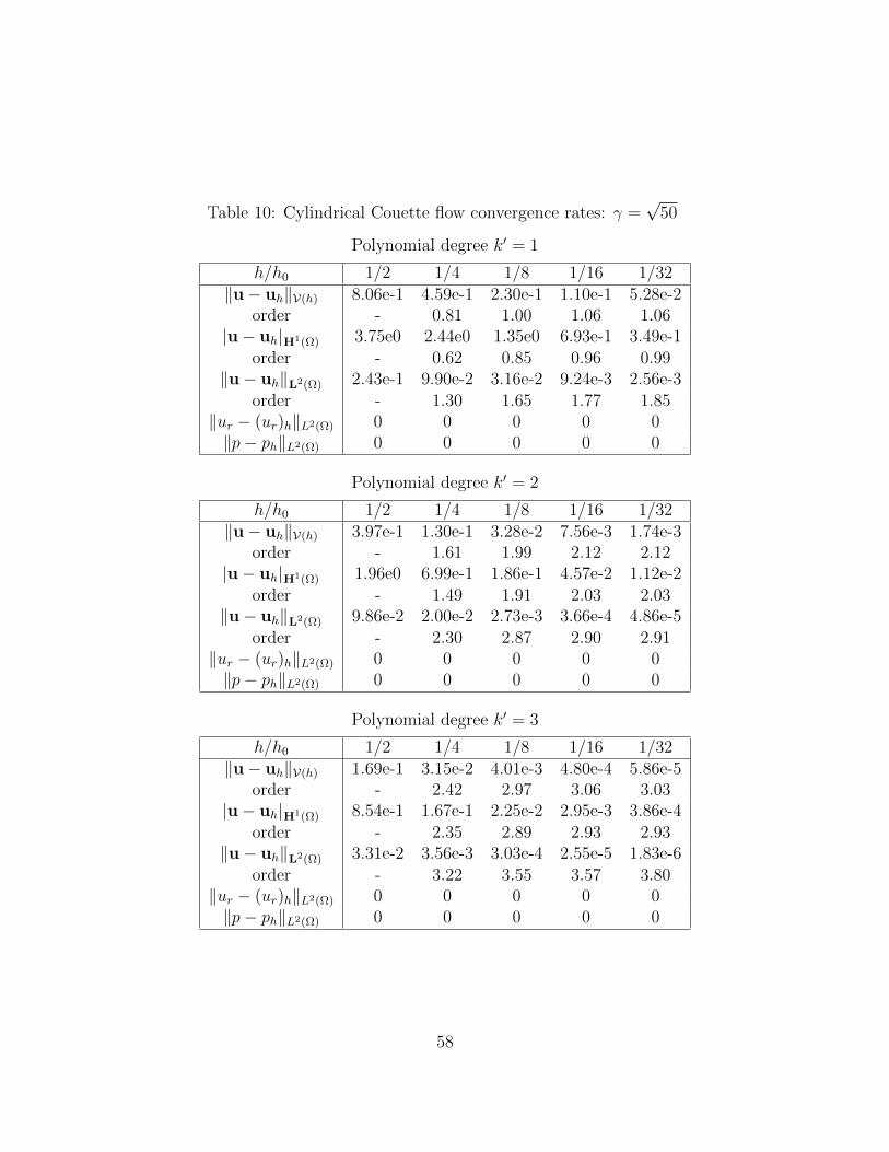
We have depicted this velocity field in Figure 14(a). In the presence of Darcy dragforces, the character of the flow field changes considerably. Notably, the motion ofthe fluid is confined to a small boundary layer attached to the inner cylinder. Thismotion explicitly takes the form

u =

[uθ(r) sin(θ)uθ(r) cos(θ)

]where

uθ(r) = UI1(γr)K1(γrout)− I1(γrout)K1(γr)

I1(γrin)K1(γrout)− I1(γrout)K1(γrin),

γ =√σ/ν, and I1 and K1 are modified Bessel functions of the first and second kind

respectively. Note that γ−1 acts as a length scale, and the width of the boundary layerattached to the inner cylinder is proportional to γ−1. We have depicted a velocityfield corresponding to γ =

√50 in Figure 14(b). Finally, under the constraint that∫

Ω

pdx = 0,

the pressure field is identically zero for both the Stokes limit as well as the generalizedStokes setting. In what follows, we assume rin = 1, rout = 2, and U = 1.

We have computed convergence rates for a variety of divergence-conforming B-spline discretizations and for γ = 0 and γ =

√50. To represent the annular domain

in our computations, we employed the polar mapping

F(ξ1, ξ2) =

[((rout − rin)ξ2 + rin) sin(2πξ1)((rout − rin)ξ2 + rin) cos(2πξ1)

],∀(ξ1, ξ2) ∈ (0, 1)2 (100)

53

rout

rin

U

Figure 13: Cylindrical Couette flow: Problem setup.

and periodic B-splines of maximal continuity in the ξ1-direction (see Section 2 of [25]).It should be emphasized that we do not use the polar form of the generalized Stokesequations. Rather, we utilize the polar mapping to define our divergence-conformingB-splines in physical space and then employ the Cartesian-based variational formu-lation discussed in this chapter. The results of our computations are summarizedin Tables 9 and 10. Note from the tables that all of our theoretically derived errorestimates are confirmed, though the results corresponding to γ =

√50 have a more

substantial pre-asymptotic range due to the presence of a boundary layer. Addition-ally, note that we obtain null pressure fields and axisymmetric velocity fields withnull radial component.

We repeated our computations using the multi-patch NURBS construction illus-trated in Figure 16. Each of the four patches are built through a sufficient rotationof the canonical quadratic single-element NURBS patch described in Figure 17, andwe have tabulated the location and weights of the control points of the canonicalquadratic patch in Figure 11. The resulting NURBS parametrization is identical tothe polar parametrization in the radial direction and different in the angular direction.We define our B-spline discretization scheme on the multi-patch NURBS construc-tion using the procedure outlined in Section 7 with normal continuity being enforcedstrongly between patches and tangential continuity being enforced weakly. Surpris-ingly, we found we obtained exactly the same velocity and pressure fields using themulti-patch NURBS construction as we did with the polar mapping. This property is

54

−2 −1.5 −1 −0.5 0 0.5 1 1.5 2−2

−1.5

−1

−0.5

0

0.5

1

1.5

2

x

y

(a)

−2 −1.5 −1 −0.5 0 0.5 1 1.5 2−2

−1.5

−1

−0.5

0

0.5

1

1.5

2

x

y

(b)

Figure 14: Cylindrical Couette flow: (a) Flow velocity arrows for γ = 0, (b) Flowvelocity arrows for γ =

√50.

55

h/h0 = 1/2

h/h0 = 1/4

h/h0 = 1/8

Figure 15: Cylindrical Couette flow: Sequence of polar meshes.

56

Table 9: Cylindrical Couette flow convergence rates: γ = 0

Polynomial degree k′ = 1

h/h0 1/2 1/4 1/8 1/16 1/32‖u− uh‖V(h) 5.42e-1 2.63e-1 1.26e-1 6.12e-2 2.99e-2

order - 1.04 1.06 1.04 1.03|u− uh|H1(Ω) 4.48e-1 2.32e-1 1.17e-1 5.86e-2 2.93e-2

order - 0.95 0.99 1.00 1.00‖u− uh‖L2(Ω) 5.00e-2 1.53-2 4.28e-3 1.14e-3 2.94e-4

order - 1.71 1.84 1.91 1.96‖ur − (ur)h‖L2(Ω) 0 0 0 0 0‖p− ph‖L2(Ω) 0 0 0 0 0

Polynomial degree k′ = 2

h/h0 1/2 1/4 1/8 1/16 1/32‖u− uh‖V(h) 9.77e-2 2.42e-2 5.64e-3 1.32e-3 3.14e-4

order - 2.01 2.10 2.10 2.07|u− uh|H1(Ω) 7.68e-2 2.00e-2 4.92e-3 1.21e-3 2.99e-4

order - 1.94 2.02 2.02 2.02‖u− uh‖L2(Ω) 4.43e-3 6.03e-4 8.13e-5 1.07e-5 1.38e-6

order - 2.88 2.89 2.93 2.95‖ur − (ur)h‖L2(Ω) 0 0 0 0 0‖p− ph‖L2(Ω) 0 0 0 0 0

Polynomial degree k′ = 3

h/h0 1/2 1/4 1/8 1/16 1/32‖u− uh‖V(h) 2.01e-2 2.67e-3 3.27e-4 4.01e-5 4.98e-6

order - 2.91 3.03 3.03 3.01|u− uh|H1(Ω) 1.52e-2 2.13e-3 2.84e-4 3.72e-5 4.80e-6

order - 2.84 2.91 2.93 2.95‖u− uh‖L2(Ω) 6.59e-4 5.69e-5 4.82e-6 3.50e-7 2.33e-8

order - 3.53 3.56 3.78 3.91‖ur − (ur)h‖L2(Ω) 0 0 0 0 0‖p− ph‖L2(Ω) 0 0 0 0 0

57

Table 10: Cylindrical Couette flow convergence rates: γ =√

50

Polynomial degree k′ = 1

h/h0 1/2 1/4 1/8 1/16 1/32‖u− uh‖V(h) 8.06e-1 4.59e-1 2.30e-1 1.10e-1 5.28e-2

order - 0.81 1.00 1.06 1.06|u− uh|H1(Ω) 3.75e0 2.44e0 1.35e0 6.93e-1 3.49e-1

order - 0.62 0.85 0.96 0.99‖u− uh‖L2(Ω) 2.43e-1 9.90e-2 3.16e-2 9.24e-3 2.56e-3

order - 1.30 1.65 1.77 1.85‖ur − (ur)h‖L2(Ω) 0 0 0 0 0‖p− ph‖L2(Ω) 0 0 0 0 0

Polynomial degree k′ = 2

h/h0 1/2 1/4 1/8 1/16 1/32‖u− uh‖V(h) 3.97e-1 1.30e-1 3.28e-2 7.56e-3 1.74e-3

order - 1.61 1.99 2.12 2.12|u− uh|H1(Ω) 1.96e0 6.99e-1 1.86e-1 4.57e-2 1.12e-2

order - 1.49 1.91 2.03 2.03‖u− uh‖L2(Ω) 9.86e-2 2.00e-2 2.73e-3 3.66e-4 4.86e-5

order - 2.30 2.87 2.90 2.91‖ur − (ur)h‖L2(Ω) 0 0 0 0 0‖p− ph‖L2(Ω) 0 0 0 0 0

Polynomial degree k′ = 3

h/h0 1/2 1/4 1/8 1/16 1/32‖u− uh‖V(h) 1.69e-1 3.15e-2 4.01e-3 4.80e-4 5.86e-5

order - 2.42 2.97 3.06 3.03|u− uh|H1(Ω) 8.54e-1 1.67e-1 2.25e-2 2.95e-3 3.86e-4

order - 2.35 2.89 2.93 2.93‖u− uh‖L2(Ω) 3.31e-2 3.56e-3 3.03e-4 2.55e-5 1.83e-6

order - 3.22 3.55 3.57 3.80‖ur − (ur)h‖L2(Ω) 0 0 0 0 0‖p− ph‖L2(Ω) 0 0 0 0 0

58

Patch 1

Patch 2

Patch 3

Patch 4

Figure 16: Cylindrical Couette flow: NURBS multi-patch construction

1 2

3

4 5

6

7 8

9

Figure 17: Cylindrical Couette flow: Patch template control points

59

Table 11: Cylindrical Couette flow: Patch template control points.

Control Point x y w1 0 1 1

2 1 1 1/√

23 1 0 14 0 3/2 1

5 3/2 3/2 1/√

26 3/2 0 17 0 2 1

8 2 2 1/√

29 2 0 1

purely a consequence of the Piola transform. To shed some light on this observation,let us consider a parametric velocity field of the form v = v(ξ2), 0T . Then, theimage of this velocity field under the Piola transform, denoted as v, has the propertythat

divv =1

Jdiv v = 0

where J is the determinant of the Jacobian matrix DF. Moreover, the vector v isoriented in the direction of parametric lines defined by ξ2 = C where C is an arbitraryconstant. Hence, if ξ1 represents the angular direction and ξ2 represents the radialdirection, this implies that divergence-free lateral velocity fields in parametric spaceare mapped to axisymmetric angular velocity fields in physical space regardless ofthe specification of F. Unfortunately, this argument applies only to angular velocityfields and we are not generally able to obtain axisymmetric pressure and radial velocityfields using the multi-patch NURBS construction.

8.5 Annular Poiseuille Flow

Poiseuille flow is another problem which is often utilized as a “sanity check” for Stokesand Navier-Stokes discretizations. Here, we consider generalized Stokes Poiseuille flowof a viscous fluid between two concentric cylinders. The problem setup is illustratedin Figure 18. No-slip and no-penetration boundary conditions are imposed alongthe cylinder surfaces, and periodic boundary conditons are imposed along the axialdirection. An external axial pressure gradient is applied to drive the fluid. In theabsence of Darcy drag forces, the velocity field for annular Poiseuille flow assumesthe form

u =

00

uz(r)

60

No-slip Walls

Periodic

BC

External Axial

Pressure Gradient

rout

rin

Inner Radius:

Outer Radius:

Cylinder Length: L

Figure 18: Annular Poiseuille flow: Problem setup.

61

where

uz(r) = − ∆p

4νL

(r2in − r2 +

r2out − r2

in

ln(rout/rin)ln(r/rin)

)(r, θ) are polar coordinates with respect to the center of the cylinders, and −∆p/L isthe applied pressure gradient. In the presence of Darcy drag, the velocity field takesthe form

u =

00

uz(r)

where

uz(r) =− ∆p

σL

(K0(γr) (I0(γrout)− I0(γrin))− I0(γr) (K0(γrout)−K0(γrin))

K0(γrout)I0(γrin)−K0(γrin)I0(γrout)

)− ∆p

σL,

γ =√σ/ν, and I0 and K0 are modified Bessel functions of the first and second kind

respectively. We have illustrated velocity fields corresponding to γ = 0 and γ =√

50in Figure 19. As was the case for cylindrical Couette flow, γ−1 acts as a length scale,and there is a boundary layer attached to the inner cylinder with width proportionalto γ−1. Finally, under the constraint that∫

Ω

pdx = 0,

the pressure field is identically zero for both the Stokes limit as well as the generalizedStokes setting. In what follows, we assume rin = 1, rout = 2, L = 1, and ∆p = −1.

We have computed convergence rates for a variety of divergence-conforming B-spline discretizations and for γ = 0 and γ =

√50. We have employed both the polar

mapping and the NURBS multi-patch construction described in the previous subsec-tion to represent the annular domain in our computations with the axial directionparametrized using a simple linear mapping. Periodic B-splines of maximal continu-ity were employed in the axial direction. The results of our computations for γ = 0are summarized in Tables 12 and 13. Note immediately that all of our theoreticallyderived error estimates are confirmed. Additionally, note that we obtain null pressurefields, radial velocity fields, and angular velocity fields for all cases considered. Thisbeing said, observe that we obtain slightly smaller axial velocity errors with the polarmapping than we do with the NURBS multi-patch construction. This is because wemaintain exact axisymmetry with the polar mapping but not with the NURBS multi-patch construction. The results of our computations for γ =

√50 are summarized

in Tables 14 and 15. Again, note that our theoretically derived error estimates areconfirmed, and our results for the polar mapping induce slightly smaller axial velocityerrors than our results for the NURBS multi-patch construction.

62

x

y

−2 −1.5 −1 −0.5 0 0.5 1 1.5 2−2

−1.5

−1

−0.5

0

0.5

1

1.5

2

0

0.02

0.04

0.06

0.08

0.1

0.12

(a)

x

y

−2 −1.5 −1 −0.5 0 0.5 1 1.5 2−2

−1.5

−1

−0.5

0

0.5

1

1.5

2

0.1

0.2

0.3

0.4

0.5

0.6

0.7

0.8

0.9

(b)

Figure 19: Annular Poiseuille flow: Axial velocity contours along an axial slice for(a) γ = 0 and (b) γ =

√50.

63

Table 12: Annular Poiseuille flow convergence rates for γ = 0: Polar meshes

Polynomial degree k′ = 1

h/h0 1/2 1/4 1/8 1/16 1/32‖u− uh‖V(h) 5.30e-1 2.47e-1 1.19e-1 5.80e-2 2.86e-2

order - 1.10 1.05 1.04 1.02|u− uh|H1(Ω) 4.56e-1 2.28e-1 1.14e-1 5.67e-2 2.83e-2

order - 1.00 1.00 1.01 1.00‖u− uh‖L2(Ω) 5.49e-2 1.62-2 4.34e-3 1.12e-3 2.84e-4

order - 1.76 1.90 1.95 1.98‖ur − (ur)h‖L2(Ω) 0 0 0 0 0‖uθ − (uθ)h‖L2(Ω) 0 0 0 0 0‖p− ph‖L2(Ω) 0 0 0 0 0

Polynomial degree k′ = 2

h/h0 1/2 1/4 1/8 1/16 1/32‖u− uh‖V(h) 5.67e-2 1.23e-2 2.83e-3 6.73e-4 1.64e-4

order - 2.20 2.12 2.07 2.04|u− uh|H1(Ω) 4.49e-2 1.07e-2 2.61e-3 6.45e-4 1.60e-4

order - 2.07 2.04 2.02 2.01‖u− uh‖L2(Ω) 2.41e-3 3.49e-4 4.64e-5 5.97e-6 7.58e-7

order - 2.79 2.91 2.96 2.98‖ur − (ur)h‖L2(Ω) 0 0 0 0 0‖uθ − (uθ)h‖L2(Ω) 0 0 0 0 0‖p− ph‖L2(Ω) 0 0 0 0 0

Polynomial degree k′ = 3

h/h0 1/2 1/4 1/8 1/16 1/32‖u− uh‖V(h) 1.86e-3 2.14e-4 2.54e-5 3.11e-6 3.87e-7

order - 3.12 3.07 3.03 3.01|u− uh|H1(Ω) 1.37e-3 1.74e-4 2.26e-5 2.93e-6 3.75e-7

order - 2.98 2.94 2.95 2.97‖u− uh‖L2(Ω) 5.38e-5 5.05e-6 4.03e-7 2.80e-8 1.83e-9

order - 3.41 3.65 3.85 3.94‖ur − (ur)h‖L2(Ω) 0 0 0 0 0‖uθ − (uθ)h‖L2(Ω) 0 0 0 0 0‖p− ph‖L2(Ω) 0 0 0 0 0

64

Table 13: Annular Poiseuille flow convergence rates for γ = 0: NURBS

Polynomial degree k′ = 1

h/h0 1/2 1/4 1/8 1/16 1/32‖u− uh‖V(h) 5.30e-1 2.47e-1 1.19e-1 5.80e-2 2.86e-2

order - 1.10 1.05 1.04 1.02|u− uh|H1(Kh) 4.57e-1 2.28e-1 1.14e-1 5.67e-2 2.83e-2

order - 1.00 1.00 1.01 1.00‖u− uh‖L2(Ω) 5.51e-2 1.63-2 4.35e-3 1.12e-3 2.84e-4

order - 1.76 1.91 1.96 1.98‖ur − (ur)h‖L2(Ω) 0 0 0 0 0‖uθ − (uθ)h‖L2(Ω) 0 0 0 0 0‖p− ph‖L2(Ω) 0 0 0 0 0

Polynomial degree k′ = 2

h/h0 1/2 1/4 1/8 1/16 1/32‖u− uh‖V(h) 5.69e-2 1.23e-2 2.83e-3 6.75e-4 1.64e-4

order - 2.21 2.12 2.07 2.04|u− uh|H1(Kh) 4.51e-2 1.07e-2 2.61e-3 6.46e-4 1.61e-4

order - 2.08 2.04 2.01 2.00‖u− uh‖L2(Ω) 2.52e-3 3.55e-4 4.70e-5 6.04e-6 7.66e-7

order - 2.83 2.92 2.96 2.98‖ur − (ur)h‖L2(Ω) 0 0 0 0 0‖uθ − (uθ)h‖L2(Ω) 0 0 0 0 0‖p− ph‖L2(Ω) 0 0 0 0 0

Polynomial degree k′ = 3

h/h0 1/2 1/4 1/8 1/16 1/32‖u− uh‖V(h) 1.91e-3 2.38e-4 2.73e-5 3.33e-6 4.13e-7

order - 3.00 3.12 3.04 3.01|u− uh|H1(Kh) 1.44e-3 2.03e-4 2.48e-5 3.16e-6 4.03e-7

order - 2.83 3.03 2.97 2.97‖u− uh‖L2(Ω) 8.00e-5 1.21e-5 6.41e-7 4.00e-8 2.53e-9

order - 2.72 4.24 4.00 3.98‖ur − (ur)h‖L2(Ω) 0 0 0 0 0‖uθ − (uθ)h‖L2(Ω) 0 0 0 0 0‖p− ph‖L2(Ω) 0 0 0 0 0

65

Table 14: Annular Poiseuille flow convergence rates for γ =√

50: Polar meshes

Polynomial degree k′ = 1

h/h0 1/2 1/4 1/8 1/16 1/32‖u− uh‖V(h) 1.73e-1 9.88e-2 4.91e-2 2.35e-2 1.13e-2

order - 0.81 1.01 1.06 1.06|u− uh|H1(Ω) 8.20e-1 5.29e-1 2.90e-1 1.48e-1 7.46e-2

order - 0.65 0.87 0.97 0.99‖u− uh‖L2(Ω) 4.88e-2 2.12-2 6.69e-3 1.94e-3 5.37e-4

order - 1.20 1.66 1.79 1.85‖ur − (ur)h‖L2(Ω) 0 0 0 0 0‖uθ − (uθ)h‖L2(Ω) 0 0 0 0 0‖p− ph‖L2(Ω) 0 0 0 0 0

Polynomial degree k′ = 2

h/h0 1/2 1/4 1/8 1/16 1/32‖u− uh‖V(h) 8.77e-2 2.59e-2 6.37e-3 1.46e-3 3.37e-4

order - 1.76 2.02 2.13 2.12|u− uh|H1(Ω) 4.34e-1 1.39e-1 3.63e-2 8.86e-3 2.16e-3

order - 1.64 1.94 2.03 2.04‖u− uh‖L2(Ω) 2.32e-2 3.98e-3 5.33e-4 7.14e-5 9.46e-6

order - 2.54 2.90 2.90 2.92‖ur − (ur)h‖L2(Ω) 0 0 0 0 0‖uθ − (uθ)h‖L2(Ω) 0 0 0 0 0‖p− ph‖L2(Ω) 0 0 0 0 0

Polynomial degree k′ = 3

h/h0 1/2 1/4 1/8 1/16 1/32‖u− uh‖V(h) 2.95e-2 5.72e-3 7.10e-4 8.48e-5 1.04e-5

order - 2.37 3.01 3.07 3.03|u− uh|H1(Ω) 1.48e-1 3.03e-2 4.02e-3 5.27e-4 6.88e-5

order - 2.29 2.91 2.93 2.94‖u− uh‖L2(Ω) 5.23e-3 6.40e-4 5.59e-5 4.63e-6 3.27e-7

order - 3.03 3.52 3.59 3.82‖ur − (ur)h‖L2(Ω) 0 0 0 0 0‖uθ − (uθ)h‖L2(Ω) 0 0 0 0 0‖p− ph‖L2(Ω) 0 0 0 0 0

66

Table 15: Annular Poiseuille flow convergence rates for γ =√

50: NURBS

Polynomial degree k′ = 1

h/h0 1/2 1/4 1/8 1/16 1/32‖u− uh‖V(h) 1.73e-1 9.88e-2 4.91e-2 2.35e-2 1.13e-2

order - 0.81 1.01 1.06 1.06|u− uh|H1(Ω) 8.20e-1 5.29e-1 2.90e-1 1.49e-1 7.46e-2

order - 0.65 0.87 0.96 1.00‖u− uh‖L2(Ω) 4.89e-2 2.12-2 6.70e-3 1.95e-3 5.37e-4

order - 1.21 1.66 1.78 1.86‖ur − (ur)h‖L2(Ω) 0 0 0 0 0‖uθ − (uθ)h‖L2(Ω) 0 0 0 0 0‖p− ph‖L2(Ω) 0 0 0 0 0

Polynomial degree k′ = 2

h/h0 1/2 1/4 1/8 1/16 1/32‖u− uh‖V(h) 8.77e-2 2.59e-2 6.38e-3 1.46e-3 3.37e-4

order - 1.76 2.02 2.13 2.12|u− uh|H1(Ω) 4.34e-1 1.39e-1 3.63e-2 8.86e-3 2.16e-3

order - 1.64 1.94 2.03 2.04‖u− uh‖L2(Ω) 2.32e-2 3.98e-3 5.33e-4 7.14e-5 9.46e-6

order - 2.54 2.90 2.90 2.92‖ur − (ur)h‖L2(Ω) 0 0 0 0 0‖uθ − (uθ)h‖L2(Ω) 0 0 0 0 0‖p− ph‖L2(Ω) 0 0 0 0 0

Polynomial degree k′ = 3

h/h0 1/2 1/4 1/8 1/16 1/32‖u− uh‖V(h) 2.95e-2 5.72e-3 7.10e-4 8.48e-5 1.04e-5

order - 2.37 3.01 3.07 3.03|u− uh|H1(Ω) 1.48e-1 3.03e-2 4.02e-3 5.27e-4 6.88e-5

order - 2.29 2.91 2.93 2.94‖u− uh‖L2(Ω) 5.23e-3 6.40e-4 5.59e-5 4.63e-6 3.27e-7

order - 3.03 3.52 3.59 3.82‖ur − (ur)h‖L2(Ω) 0 0 0 0 0‖uθ − (uθ)h‖L2(Ω) 0 0 0 0 0‖p− ph‖L2(Ω) 0 0 0 0 0

67

H

H

U

Figure 20: Lid-driven Stokes flow in a two-dimensional cavity: Problem setup.

9 Benchmark Problems

In this section, we investigate the effectiveness of our methodology as applied to twostandard Stokes benchmark problems: two-dimensional and three-dimensional lid-driven cavity flow. In addition, we investigate the effectiveness of our methodology fora Darcy-dominated generalized Stokes flow problem characterized by sharp boundarylayers. As in the last subsection, we choose Nitsche’s penalty constant as Cpen =5(k′ + 1) in all of the following numerical tests, and we employ uniform parametricmeshes, linear parametric mappings, and B-spline spaces of maximal continuity.

9.1 Two-Dimensional Lid-Driven Cavity Flow

Two-dimensional lid-driven cavity flow is one of the classical verification tests fornumerical discretizations of incompressible flow. The setup for this flow problem iselaborated in Figure 20. The reaction coefficient σ and the applied forcing f are setto be zero. The left, right, and bottom sides of the cavity are fixed no-slip walls whilethe top side of the cavity is a wall which slides to the right with velocity magnitudeU . For the computations here, H and U are set to be 1. The pressure and stress fieldsassociated with this flow experience corner singularities which impede the convergenceof numerical methods and expose unstable velocity/pressure pairs. In fact, the exactvelocity solution does not even lie in H1(Ω). Instead, it lies in the Sobolev space

68

W1,q(Ω) where 1 < q < 2. The velocity field is additionally characterized by aprimary vortex near the center of the cavity and an infinite sequence of so-calledMoffatt eddies of decreasing size and intensity in the lower left and right corners of thecavity [47]. Of primary interest is how well our discretization procedure approximatesthe smooth portions of the flow. Of secondary interest is how well our discretizationprocedure resolves the corner singularities. We do not, however, employ any specialtechniques such as singular finite elements to handle the singularities.

We have computed approximations of two-dimensional lid-driven cavity flow usingdivergence-conforming B-spline discretizations of varying mesh size and polynomialdegrees k′ = 1, 2, 3. The computed streamlines for two of these approximations arepresented in Figure 21. The streamlines corresponding to the approximation definedon the fine mesh (k′ = 1, h = 1/128) are virtually indistinguishable from well-acceptedbenchmark solutions [51]. The streamlines corresponding to the approximation de-fined on the coarse mesh (k′ = 1, h = 1/16) closely resemble the fine mesh streamlinesin the interior of the domain. In the four corners of the domain, the approximationon the coarse mesh exhibits visible numerical error due to lack of resolution. Theseresults indicate that our methodology suffers from minimal pollution error [4]. It ishypothesized that this is due to the local stability and approximation properties ofB-splines. To further highlight how well the approximation on the coarse mesh ap-proximates the solution in the interior of the domain, we have plotted the value of thefirst component of the velocity field along the vertical center line in Figure 22(a) andthe value of the second component along the horizontal center line in Figure 22(b)for the both the coarse mesh and fine mesh solutions. It should be mentioned thatwe have captured the first Moffatt eddy in the two lower corners with both meshes,and we have observed a second Moffatt eddy for meshes of size h ≤ 1/256.

We finish our discussion of the two-dimensional lid-driven cavity problem by an-alyzing how well our methodology resolves the corner singularities. To do so, wecompare the results of our methodology with the highly accurate pseudospectral re-sults given in [10]. These pseudospectral results were obtained using a subtraction ofthe leading terms of the asymptotic solution of the Stokes equations in the vicinityof the corners in order to exactly represent the corner singularities. In Table 16,we compare the vorticity (ω = curlu) given by our numerical methodology with thepseudospectral vorticity near the upper right corner of the cavity. We see that thevorticity associated with our numerical methodology slowly converges to the con-verged pseudospectral solution. We further compare our computed vorticities withthe vorticity obtained with a highly-refined finite difference solution [32]. We findthat, for k′ = 1, our solutions are more accurate than the finite difference solution forh ≤ 1/64, and for k′ = 2, our solutions are more accurate than the finite differencesolution for h ≤ 1/32. For k′ = 3, our solutions are more accurate than the finitedifference solution at all resolutions.

69

x

y

0 0.1 0.2 0.3 0.4 0.5 0.6 0.7 0.8 0.9 10

0.1

0.2

0.3

0.4

0.5

0.6

0.7

0.8

0.9

1

(a)

x

y

0 0.1 0.2 0.3 0.4 0.5 0.6 0.7 0.8 0.9 10

0.1

0.2

0.3

0.4

0.5

0.6

0.7

0.8

0.9

1

(b)

Figure 21: Lid-driven Stokes flow in a two-dimensional cavity: (a) Computed flowvelocity streamlines for k′ = 1 and h = 1/16, (b) Computed flow velocity streamlinesfor k′ = 1 and h = 1/128.

70

0.4 0.2 0 0.2 0.4 0.6 0.8 10

0.1

0.2

0.3

0.4

0.5

0.6

0.7

0.8

0.9

1

u/U

y/H

h = 1/16h = 1/128

(a)

0 0.2 0.4 0.6 0.8 10.2

0.15

0.1

0.05

0

0.05

0.1

0.15

0.2

x/H

v/U

h = 1/16h = 1/128

(b)

Figure 22: Lid-driven Stokes flow in a two-dimensional cavity: (a) Value of the firstcomponent of the velocity field along the vertical center line for k′ = 1, (b) Value ofthe second component of the velocity field along the horizontal center line for k′ = 1.

71

Table 16: Lid-driven Stokes flow in a two-dimensional cavity: Convergence of vorticityat the point (x = (1, 0.95)).

Polynomial degree k′ = 1

Method ωB-spline, h = 1/16 −0.80995B-spline, h = 1/32 14.34482B-spline, h = 1/64 19.04468B-spline, h = 1/128 23.29179B-spline, h = 1/256 25.32238

Pseudospectral (Ref. [10]) 27.27901Finite Difference (Ref. [32]) 18.08

Polynomial degree k′ = 2

Method ωB-spline, h = 1/16 11.06384B-spline, h = 1/32 31.81761B-spline, h = 1/64 32.81972B-spline, h = 1/128 26.48645B-spline, h = 1/256 27.34395

Pseudospectral (Ref. [10]) 27.27901Finite Difference (Ref. [32]) 18.08

Polynomial degree k′ = 3

Method ωB-spline, h = 1/16 29.86220B-spline, h = 1/32 25.00897B-spline, h = 1/64 29.92944B-spline, h = 1/128 28.75895B-spline, h = 1/256 27.52637

Pseudospectral (Ref. [10]) 27.27901Finite Difference (Ref. [32]) 18.08

72

H

H

U H

z y

x

Figure 23: Lid-driven Stokes flow in a three-dimensional cavity: Problem setup.

9.2 Three-Dimensional Lid-Driven Cavity Flow

While three-dimensional lid-driven cavity flow is encountered much less often in theliterature than its two-dimensional counterpart, we believe it is still an interesting testcase for numerical discretizations of incompressible flow. In the three-dimensional set-ting, cavity flow is characterized by the presence of both edge and corner singularities.The problem setup is illustrated in Figure 23. Again, for the computations here, σand f are set to be zero. Every side of the cavity except the top is assumed to bea stationary no-slip wall, and the top side of the cavity is assumed to be a wallwhich slips to the right with velocity magnitude U . The streamlines resulting from asimulation of three-dimensional lid-driven cavity flow using divergence-conforming B-splines of degree k′ = 2 on a mesh with 32× 32 elements are illustrated in Figure 24.Note that the three-dimensional streamlines resemble the two-dimensional stream-lines along the slice y/H = 1/2. To examine how well our discretization techniqueperforms on coarse meshes, we have compared the centerline values of our velocityfield along the slice y/H = 1/2 for both a coarse and fine mesh approximation inFigure 25. From the figure, we see that the coarse and fine mesh centerline velocityfields are nearly indistinguishable. This indicates that our methodology suffers fromminimal pollution error.

73

Figure 24: Lid-driven Stokes flow in a three-dimensional cavity: Computed flowvelocity streamlines for k′ = 2 and h = 1/32 colored by velocity magnitude.

9.3 Darcy-Dominated Flow with Sharp Boundary Layers

As a final numerical example, we consider a reaction-dominated generalized Stokesproblem subject to sharp boundary layers. The problem is posed on the unit square.Homogeneous no-slip and no-penetration boundary conditions are enforced along theboundary of the square, and an external forcing of the form

f =

[sin(πx) cos(πy)− cos(πx) sin(πy)

]is applied. The reaction term σ is set to be equal to 1 while the viscosity ν is set tobe equal to 10−6. With these choices, the resulting flow field has a vortical structurein the interior of the domain and sharp boundary layers along the entire boundary ofthe domain.

We have simulated this flow problem using both our discretization technique aswell as the Q2/Q1 Taylor-Hood velocity/pressure pair [36]. The Taylor-Hood veloc-ity/pressure pair is one of the most popular finite elements for generalized Stokes flow,but it is known not to be robust in the Darcy limit. Specifically, the accuracy of theQ2/Q1 Taylor-Hood velocity field reduces to first-order in the Darcy limit [33]. This isdue to a lack of strong coercivity (in the kernel) with respect to the H(div; Ω)-norm.We have visualized the computed velocity vectors corresponding to divergence-freeB-splines of degree k′ = 1 and the Q2/Q1 Taylor-Hood velocity-pressure pair on a16× 16 element mesh in Figures 26(a) and (b). These two quiver plots seem to indi-cate that the two discrete flow fields are nearly identical except in a small region near

74

−0.4 −0.2 0 0.2 0.4 0.6 0.8 10

0.1

0.2

0.3

0.4

0.5

0.6

0.7

0.8

0.9

1

u/U

z/H

h = 1/16h = 1/64

(a)

0 0.2 0.4 0.6 0.8 1−0.2

−0.15

−0.1

−0.05

0

0.05

0.1

0.15

0.2

x/H

w/U

h = 1/16h = 1/64

(b)

Figure 25: Lid-driven Stokes flow in a three-dimensional cavity: (a) Value of the firstcomponent of the velocity field along the line (x/H, y/H) = (1/2, 1/2) for k′ = 1,(b) Value of the third component of the velocity field along the line (y/H, z/H) =(1/2, 1/2) for k′ = 1.

75

the boundary of the domain. However, when we view only the first-component of thevelocity field as in Figures 27 and 28, we see that the divergence-free B-spline solu-tion is monotone while the Taylor-Hood solution suffers from spurious oscillations.Finally, we have visualized the divergence of the discrete flow field corresponding tothe Taylor-Hood solution in Figure 29. From this figure, we see that the Taylor-Hoodsolution is characterized by strong expansion and compression in the four corners ofthe domain. When coupled with a transport solver, this ultimately leads to methodswith unphysical species production [46]. On the other hand, the discrete flow fieldcorresponding to the B-spline solution is pointwise divergence-free.

10 Conclusions

In this paper, new divergence-conforming B-spline discretizations have been presentedfor the generalized Stokes equations. A collection of stability and error estimates havebeen derived which are robust with respect to the parameters of generalized Stokesflow, and these theoretical results have been confirmed and supplemented by numer-ical simulations of problems with known analytical solutions. These discretizationshave been also applied to the simulation of a number of benchmark problems wherethe advantages of the new methodology over classical methods have been highlighted.In future work, we plan to extend the present developments to the Navier-Stokesequations and generalize to locally-refined meshes.

Acknowledgements

John A. Evans and Thomas J.R. Hughes were partially supported by the Office ofNaval Research under contract number N00014-08-0992 and by the National ScienceFoundation under Grant No. 0700204. John A. Evans was additionally partiallysupported by the Department of Energy Computational Science Graduate Fellow-ship, provided under grant number DE-FG02-97ER25308. This support is gratefullyacknowledged.

References

[1] D N Arnold. An interior penalty finite element method with discontinuous ele-ments. SIAM Journal on Numerical Analysis, 19:742–760, 1982.

[2] D N Arnold and J Qin. Quadratic velocity/linear pressure Stokes elements. InR Vichnevetsky and R S Steplemen, editors, Advances in Computer Methods forPartial Differential Equations VII, 1992.

76

[3] I Babuska. Error bounds for finite element method. Numerische Mathematik,16:322–333, 1971.

[4] I Babuska and H-S Oh. Pollution problem of the p- and h − p versions of thefinite element method. Numerical Methods in Biomedical Engineering, 3:553–561, 1987.

[5] Y Bazilevs, V M Calo, J A Cottrell, J A Evans, T J R Hughes, S Lipton, M AScott, and T W Sederberg. Isogeometric analysis using T-splines. ComputerMethods in Applied Mechanics and Engineering, 199:229–263, 2010.

[6] Y Bazilevs and T J R Hughes. Weak imposition of Dirichlet boundary conditionsin fluid mechanics. Computers and Fluids, 36:12–26, 2007.

[7] Y Bazilevs, C M Michler, V M Calo, and T J R Hughes. Weak Dirichlet bound-ary conditions for wall-bounded turbulent flows. Computer Methods in AppliedMechanics and Engineering, 196:4853–4862, 2007.

[8] Y Bazilevs, C M Michler, V M Calo, and T J R Hughes. Isogeometric varia-tional multiscale modeling of wall-bounded turbulent flows with weakly-enforcedboundary conditions on unstretched meshes. Computer Methods in Applied Me-chanics and Engineering, 199:780–790, 2010.

[9] D Boffi, F Brezzi, and M Fortin. Finite elements for the Stokes problem. LectureNotes in Mathematics, 1939:45–100, 2008.

[10] O Botella and R Peyret. Benchmark spectral results on the lid-driven cavityflow. Computers and Fluids, 27:421–433, 1998.

[11] S C Brenner. Korn’s inequalities for piecewise H1 vector fields. Mathematics ofComputation, 73:1067–1087, 2003.

[12] F Brezzi. On the existence, uniqueness and approximation of saddle-point prob-lems arising from Lagrange multipliers. Revue Francaise d’Automatique Infor-matique et Recherche Operationnellle. Analyse Numerique, 8:129–151, 1974.

[13] H C Brinkman. A calculation of the viscous force exerted by a flowing fluid ona dense swarm of particles. Applied Scientific Research, A1:27–34, 1947.

[14] A Buffa, C de Falco, and R Vazquez. Isogeometric analysis: Stable elements forthe 2D Stokes equation. International Journal for Numerical Methods in Fluids,65:1407–1422,20–30, 2011.

[15] A Buffa, J Rivas, G Sangalli, and R Vazquez. Isogeometric discrete differentialforms in three dimensions. SIAM Journal on Numerical Analysis, 49:818–844,2011.

77

[16] A Buffa, G Sangalli, and R Vazquez. Isogeometric analysis in electromagnetics:B-splines approximation. Computer Methods in Applied Mechanics and Engi-neering, 199:1143–1152, 2010.

[17] B Cockburn and J Gopalakrishnan. Incompressible finite elements via hybridiza-tion. Part I: The Stokes system in two space dimensions. SIAM Journal onNumerical Analysis, 43:1627–1650, 2005.

[18] B Cockburn and J Gopalakrishnan. Incompressible finite elements via hybridiza-tion. Part II: The Stokes system in three space dimensions. SIAM Journal onNumerical Analysis, 43:1651–1672, 2005.

[19] B Cockburn, G Kanschat, and D Schotzau. A note on discontinuous Galerkindivergence-free solutions of the Navier-Stokes equations. SIAM Journal on Sci-entific Computing, 31:61–73, 2007.

[20] J A Cottrell, T J R Hughes, and Y Bazilevs. Isogeometric Analysis: TowardIntegration of CAD and FEA. Wiley, 2009.

[21] L Beirao da Veiga, A Buffa, J Rivas, and G Sangalli. Some estimates for h−p−krefinement in isogeometric analysis. Numerische Mathematik, 118:271–305, 2011.

[22] D B Das. Hydrodynamic modelling for groundwater flow through permeablereactive barriers. Hydrodynamics Processes, 16:3393–3418, 2002.

[23] C R de Boor. A Practical Guide to Splines. Springer-Verlag, 1978.

[24] J Douglas and T Dupont. Interior Penalty Procedures for Elliptic and ParabolicGalerkin Methods. Lecture Notes in Physics, 58, 1976.

[25] J A Evans, Y Bazilevs, I Babuska, and T J R Hughes. n-widths, sup-infs, andoptimality ratios for the k-version of the isogeometric finite element method.Computer Methods in Applied Mechanics and Engineering, 198:1726–1741, 2009.

[26] J A Evans and T J R Hughes. Explicit trace inequalities for isogeometric analysisand parametric finite elements. Technical report, ICES Report 11-17, 2011.

[27] L P Franca and T J R Hughes. Two classes of mixed finite element methods.Computer Methods in Applied Mechanics and Engineering, 69:89–129, 1988.

[28] J Gerbeau, C L Bris, and M Bercovier. Spurious velocities in the steady flow ofan incompressible fluid subjected to external forces. International Journal forNumerical Methods in Fluids, 25:679–695, 1997.

[29] V Girault and P A Raviart. Finite Element Methods for Navier-Stokes Equations.Theory and Algorithms. Springer-Verlag, 1986.

78

[30] W Gui and I Babuska. The h, p and hp versions of the finite element methodin one dimension. Part 1: The error analysis of the p-version. Part 2: The erroranalysis of the h- and hp-versions. Part 3: The adaptive hp version. NumerischeMathematik, 49:577–683, 1986.

[31] G Guo and I Babuska. The hp version of the finite element method. Part 1: Thebasic approximation results. Part 2: General results and applications. Compu-tational Mechanics, 1:21–41,203–220, 1986.

[32] M M Gupta. A comparison of numerical solutions of convective and divergenceforms of the Navier-Stokes equations for the driven cavity problem. Journal ofComputational Physics, 43:260–267, 1981.

[33] A Hannukainen, M Juntunen, and R Stenberg. Computations with finite elementmethods for the Brinkman problem. Computational Geosciences, 15:155–166,2010.

[34] F H Harlow and J E Welch. Numerical calculation of time-dependent viscousincompressible flow of fluid with free surface. Physics of Fluids, 8:2182, 1965.

[35] K Hollig. Finite Element Methods with B-splines. Society for Industrial andApplied Mathematics, 2003.

[36] P Hood and C Taylor. Navier-Stokes equations using mixed interpolation. In J TOden, R H Gallagher, O C Zienkiewicz, and C Taylor, editors, Finite ElementMethods in Flow Problems, pages 121–132. University of Alabama in HuntsvillePress, 1974.

[37] T J R Hughes, L P Franca, and M Balestra. A new finite element formulation forcomputational fluid dynamics: V. Circumventing the Babuska-Brezzi condition:A stable Petrov-Galerkin formulation of the Stokes problem accomodating equal-order interpolations. Computer Methods in Applied Mechanics and Engineering,59:85–99, 1986.

[38] G Kanschat. Divergence-free discontinuous Galerkin schemes for the Stokes equa-tions and the MAC scheme. International Journal for Numerical Methods inFluids, 56:941–950, 2008.

[39] T Kara and J Goldak. Three-dimensional numerical analysis of heat and masstransfer in heat pipes. Heat Mass Transfer, 43:775–785, 2007.

[40] A-R A Khaled and K Vafai. The role of porous media in modeling flow and heattransfer in biological tissues. International Journal of Heat and Mass Transfer,46:4989–5003, 2003.

79

[41] B J Kirby. Micro- and Nanoscale Fluid Mechanics: Transport in MicrofluidicDevices. Cambridge University Press, 2010.

[42] J Konno and R Stenberg. Non-conforming finite element method for theBrinkman problem. In G Kreiss, P Lotstedt, A Malqvist, and M Neytcheva,editors, Numerical Mathematics and Advanced Applications, 2010.

[43] P G Lemaire-Rieusset. Analyses multi-resolutions non orthogonales, commu-tation entre projecteurs et derivation et ondelettes vecteurs a divergence nulle.Revista Matematica Iberoamericana, 8:221–237, 1992.

[44] A Linke. Collision in a cross-shaped domain - A steady 2d Navier-Stokes exampledemonstrating the importance of mass conservation in CFD. Computer Methodsin Applied Mechanics and Engineering, 198:3278–3286, 2009.

[45] K A Mardal, X-C Tai, and R Winther. A robust finite element method forDarcy-Stokes flow. SIAM Journal on Numerical Analysis, 40:1605–1631, 2002.

[46] G Matthies and L Tobiska. Mass conservation of finite element methods forcoupled flow-transport problems. International Journal for Computing Scienceand Mathematics, 1:293–307, 2007.

[47] H K Moffatt. Viscous and resistive eddies near a sharp corner. Journal of FluidMechanics, 64:1–18, 1964.

[48] J A Nitsche. Uber ein Variationspringzip zur Losung von Dirichlet-Problemembei Verwendung von Teilraumen, die keinen Randbedingungen unterworfen sind.Abhandlungen aus dem Mathematischen Seminar der Universit at Hamburg,36:9–15, 1971.

[49] P A Raviart and J M Thomas. A mixed finite element method for second orderelliptic problems. Lecture Notes in Mathematics, 606:292–315, 1977.

[50] B Riviere and M F Wheeler. A discontinuous Galerkin method applied to non-linear parabolic equations. Lecture Notes in Computational Science and Engi-neering, 11:231–244, 2000.

[51] W W Schultz, N T Lee, and J P Boyd. Chebyshev pseudospectral method ofviscous flows with corner singularities. Journal of Scientific Computing, 4:1–24,1989.

[52] L L Schumaker. Spline functions: Basic theory. Cambridge Mathematical Li-brary, Cambridge University Press, 2007.

[53] L R Scott and M Vogelius. Norm estimates for a maximal right inverse of thedivergence operator in spaces of piecewise polynomials. Mathematical Modellingand Numerical Analysis, 19:111–143, 1985.

80

[54] G Stadler, M Gurnis, C Burstedde, L C Wilcox, L Alisic, and O Ghattas. Thedynamics of plate tectonics and mantle flow: From local to global scales. Science,329:1033–1038, 2010.

[55] R Stevenson. Divergence-free wavelet bases on the hypercube: Free-slip bound-ary conditons, and applications for solving the instationary Stokes equations.Mathematics of Computation, 80:1499–1523, 2011.

[56] X-C Tai and R Winther. A discrete de Rham complex with enhanced smoothness.CALCOLO, 43:287–306, 2006.

[57] H Triebel. Interpolation Theory, Function Spaces, Differential Operators, SecondEdition. Johann Ambrosius Barth, 1995.

[58] K Urban. Wavelet bases in H(div) and H(curl). Mathematics of Computation,70:739–766, 2001.

[59] K Urban. Wavelets in Numerical Simulation: Problem Adapted Constructionand Applications. Springer-Verlag, 2002.

[60] R Verurth. A Review of a Posteriori Error Estimation and Adaptive Mesh-Refinement Techniques. B.G. Teubner, 1996.

[61] J Wang and X Ye. New finite element methods in computational fluid dynamicsby H(div) elements. SIAM Journal on Numerical Analysis, 45:1269–1286, 2007.

[62] M F Wheeler. An elliptic collocation-finite element method with interior penal-ties. SIAM Journal on Numerical Analysis, 15:152–161, 1978.

[63] S Zhang. A new family of stable mixed finite elements for 3D Stokes equations.Mathematics of Computation, 250:543–554, 2005.

81

0 0.2 0.4 0.6 0.8 10

0.1

0.2

0.3

0.4

0.5

0.6

0.7

0.8

0.9

1

x

y

(a)

0 0.2 0.4 0.6 0.8 10

0.1

0.2

0.3

0.4

0.5

0.6

0.7

0.8

0.9

1

x

y

(b)

Figure 26: Darcy-dominated flow with boundary layers: Computed velocity fields: (a)Divergence-free B-splines of degree k′ = 1, (b) Q2/Q1 Taylor-Hood velocity/pressurepair.

82

(a)

(b)

Figure 27: Darcy-dominated flow with boundary layers: First-component of the ve-locity field: (a) Divergence-free B-splines of degree k′ = 1, (b) Q2/Q1 Taylor-Hoodvelocity/pressure pair.

83

(a)

(b)

Figure 28: Darcy-dominated flow with boundary layers: Cross-section view of thefirst velocity component from the y = 1 line: (a) Divergence-free B-splines of degreek′ = 1, (b) Q2/Q1 Taylor-Hood velocity/pressure pair.

84

x

y

0 0.2 0.4 0.6 0.8 10

0.2

0.4

0.6

0.8

1

−2

−1.5

−1

−0.5

0

0.5

1

1.5

2

Figure 29: Darcy-dominated flow with boundary layers: Divergence of the discreteflow field corresponding to the Q2/Q1 Taylor-Hood velocity/pressure pair.

85