ICT International Doctoral School Randomized Algorithms...

ICT International Doctoral School, Trento @RT 2014

ICT International Doctoral School

Department of Information Engineering and Computer Science

University of Trento


Randomized Algorithms for Systems, Control and Networks

Roberto TempoCNR-IEIIT

Consiglio Nazionale delle Ricerche

Politecnico di Torino

[email protected]


Objective and Prerequisites

Objective: introduction to general purpose methods of randomization for analysis and design of uncertain systems

Prerequisites: basic knowledge of probability theory and familiarity with state space methods for control system analysis and design


Course and Slides

The course consists of three distinct sections

- analysis

- design

- networks

The slides include more material than that presented in the course

pdf file with slides are provided


Final Project

Course grade based on a final project to be discussed


Schedule

Monday 15:00-17:00Tuesday 9:00-12:00 and 15:00-17:00Wednesday 9:00-12:00 and 15:00-17:00Thursday 9:00-12:00 and 15:00-17:00 Friday 9:00-12:00


Main References - 1

R. Tempo, G. Calafiore and F. Dabbene,

“Randomized Algorithms for Analysis

and Control of Uncertain Systems, with

Applications,” Second Edition,

Springer-Verlag, London, 2013

F. Dabbene and R. Tempo, “Randomized Methods for

Control,” Encyclopedia of Systems and Control, 2014

(to appear)


Main References - 2

F. Dabbene and R. Tempo, “Probabilistic and

Randomized Tools for Control Design,” The Control

Handbook, second edition, Taylor & Francis, 2010

G. Calafiore, F. Dabbene and R. Tempo “Research on

Probabilistic Design Methods,” Automatica, 2011

R. Tempo and H. Ishii, “Monte Carlo and Las Vegas

Randomized Algorithms for Systems and Control: An

Introduction,” European Journal of Control, 2007


Software

R-RoMulOC: Randomized and Robust Multi-Objective

Control toolbox

http://projects.laas.fr/OLOCEP/rromuloc/

RACT: Randomized Algorithms Control Toolbox for

Matlab

http://ract.sourceforge.net


Research Interests and Background

Question: What are your research interests andbackground?


Main Topics Studied in this Course

Preliminaries

Probabilistic Analysis

Probabilistic Design: The Big Picture

Sequential Methods for Convex Problems

Non-Sequential Methods

RACT

Opinion dynamics in social networks

PageRank computation in Google

Sensor localization in wireless networks


Part 1: Analysis

Analysis Paradigm:

Understanding Phenomena


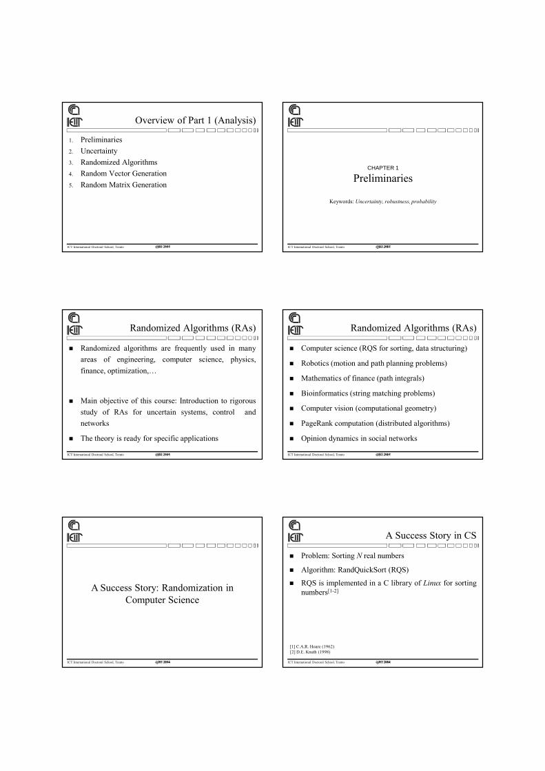
Overview of Part 1 (Analysis)

1. Preliminaries

2. Uncertainty

3. Randomized Algorithms

4. Random Vector Generation

5. Random Matrix Generation


CHAPTER 1

Preliminaries

Keywords: Uncertainty, robustness, probability


Randomized Algorithms (RAs)

Randomized algorithms are frequently used in many

areas of engineering, computer science, physics,

finance, optimization,…

Main objective of this course: Introduction to rigorous

study of RAs for uncertain systems, control and

networks

The theory is ready for specific applications


Randomized Algorithms (RAs)

Computer science (RQS for sorting, data structuring)

Robotics (motion and path planning problems)

Mathematics of finance (path integrals)

Bioinformatics (string matching problems)

Computer vision (computational geometry)

PageRank computation (distributed algorithms)

Opinion dynamics in social networks


A Success Story: Randomization in Computer Science


A Success Story in CS

Problem: Sorting N real numbers

Algorithm: RandQuickSort (RQS)

RQS is implemented in a C library of Linux for sortingnumbers[1-2]

[1] C.A.R. Hoare (1962)[2] D.E. Knuth (1998)


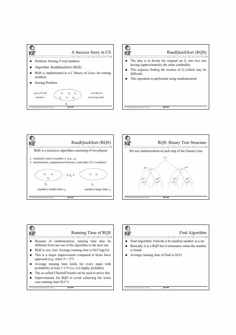
A Success Story in CS

Problem: Sorting N real numbers

Algorithm: RandQuickSort (RQS)

RQS is implemented in a C library of Linux for sortingnumbers

Sorting Problem

given N real x1 x2 x3 sort them in

numbers x4 x5 x6 increasing order

S1ICT International Doctoral School, Trento @RT 2014

RandQuickSort (RQS)

The idea is to divide the original set S1 into two setshaving (approximately) the same cardinality

This requires finding the median of S1 (which may bedifficult)

This operation is performed using randomization


RandQuickSort (RQS)

RQS is a recursive algorithm consisting of two phases

1. randomly select a number xi (e.g. x4)2. deterministic comparisons between xi and other (N-1) numbers

x2 x3 x1 x5

x6

numbers smaller than x4 numbers larger than x4

S2 S3

4x


RQS: Binary Tree Structure

We use randomization at each step of the (binary) tree


Running Time of RQS

Because of randomization, running time may bedifferent from one run of the algorithm to the next one

RQS is very fast: Average running time is O(N log(N))

This is a major improvement compared to brute forceapproach (e.g. when N = 2M)

Average running time holds for every input withprobability at least 1-1/N (i.e. it is highly probable)

The so-called Chernoff bound can be used to prove this

Improvements for RQS to avoid achieving the worstcase running time O(N 2)


Find Algorithm

Find Algorithm: Find the k-th smallest number in a set

Basically it is a RQS but it terminates when the numberis found

Average running time of Find is O(N)


Another Success Story: Randomization in Mathematical Finance


(Quasi) Monte Carlo Methods for Computational Finance

QMC methods to estimate the prize of collaterizedmortgage obligations

The problem is to approximate the average mortgage

taking N samples for each variable, but we need Nn

total number of points

Curse of dimensionality: n = 360!

[0,1]( ) d

nf u u


Uncertainty and Robustness

Some History


Uncertainty

“The use of equalizing structures to compensate for the variation

in the phase and attenuation characteristics of transmission lines

and other pieces of apparatus is well known in the communication

art… the characteristics demanded of the equalizer cannot be

prescribed in advance, either because… are not known with

sufficient precision, or because they vary with time… transmission

lines the exact lengths of which are unknown, or the

characteristics of which may be affected by changes in

temperature and humidity.... and since the daily cycle of

temperature changes may be large…”


Variable Equalizers

The quote is taken from the paper titled “Variable

Equalizers” by Hendrik W. Bode published in 1938 in

Bell System Technical Journal

The quote continues “it is almost essential that theadjustments made be so simple that they can readily beperformed automatically by a suitable auxiliary circuit.”

Bode fully recognized the importance to control a systemsubject to uncertainty


Robustness

The examination of uncertainty in the mathematical

model of a system is known as robustness

Uncertainty is a central part of feedback and controllers

which guarantee an adequate level of performance are

called robust controllers


History

Classical sensitivity period (before 1960)

State-variable period (1960-1975)

Modern robust control period (after 1975)


Two Lines of Research in the Early Seventies

Design of adaptive guaranteed cost control in the

presence of large parameter variations[1]

Set-theoretic description of uncertainty (called

unknown-but-bounded) for estimation problems[2]

[1] S. Chang and T.K.C. Peng (1972)

[2] F. Schweppe (1973)


Other Early Approaches where “Robust” Appeared

Robust controllers for linear regulators[1]

Robust control of general servomechanisms[2]

[1] J. Pearson and P.W. Staats (1974)

[2] E. Davison and A. Goldenberg (1975)


Robustness and H Control

Lack of guaranteed robustness margins in LQG

control[1]

Robustness of systems with sector-type uncertainty[2]

Major stepping stone in 1981 by George Zames:

Formulation of the H control problem and solution of

the H sensitivity problem[3]

[1] J. Doyle (1978)

[2] M.G. Safonov (1980)

[3] G. Zames (1981)


State Space Approach and Solution

Performance limitations in feedback control[1]

Further developments based on interpolation theory[2]

… but the theory moved in a state space direction[3]

[1] J. Freudenberg and D. Looze (1985)

[2] G. Zames and B. A. Francis (1983)

[3] J. C. Doyle, K. Glover, P. P. Khargonekar and B. Francis (1989)


Today

Various “robust” methods to handle uncertainty now

exist: Structured singular values, Kharitonov,

optimization-based (LMI and SOS), integral quadratic

constraints (IQC), ℓ-one optimal control, quantitative

feedback theory (QFT), probabilistic/randomized

methods


Automatica 50th Anniversary

I.R. Petersen and R. Tempo, “Robust Control of

Uncertain Systems: Classical Results and Recent

Developments,” Automatica, 2014 (to appear)ICT International Doctoral School, Trento @RT 2014

Example: H Performance


Consider the linear system

with (nominal) parameters

a0 = 1 a1 = 0.8

The transfer function z = G(s) w is given by

Example: Frequency Response

0 1

0 1 0 0

1 1x x u w

a a

1 0z x

2

1( )

0.8 1G s

s s

disturbances

errors

w

z


H performance

||G(s)|| = sup |G(j)| ≤ γ

Performance is satisfied for γ = 1.35

Example: H Norm

Bode plot (magnitude)


System Performance with Uncertainty

Consider an uncertain stable transfer function G(s,q)

z = G(s,q) w

where w and z are disturbances and errors and qrepresents uncertainty bounded in a set Q of radius ρ > 0

G(s,q) w z


Consider the uncertain linear system

with parameters

a0 = 1 + q0 a1 = 0.8 + q1

and bounding set

Q = {q = [q0 q1 ]T : ||q|| }

Example[1]: System Performance with Uncertainty

0 1

0 1 0 0

1 1x x u w

a a

1 0z x

[1] R. Tempo, G. Calafiore, F. Dabbene (2013)


Given performance level the objective is tocompute the maximal radius of Q such that

G(s,q) is stable and ||G(s,q)|| for all q Q

G(s,q) is stable and ||G(s,q)|| if and only if

< 0.8 and

Example: Radius of Uncertainty

2(0 .8 ρ )1 ρ

2 2

ργ= 2


Example: Radius of Uncertainty

Largest radius of Q suchthat performance is satisfied is = 0.025

Conclusion: Stability and performance are satisfied for all q Qwith radius = 0.025

ρ

ρ


CHAPTER 2

Robustness

Keywords: parametric and nonparametric uncertainty


Uncertain Linear Systems

M(s) UncertaintySystem

belongs to a structured set B

– Parametric uncertainty q

– Nonparametric uncertainty np

– Mixed uncertainty


Worst Case Model

Worst case model: Set membership uncertainty

The uncertainty is bounded in a set B

B

Real parametric uncertainty q=[q1,…, q] R

qi [qi-, qi

+]

Nonparametric uncertainty

{np Rn,n : || np || 1}


Robustness

Uncertainty is bounded in a structured set B

z = Fu(M,) w, where Fu(M,) is the upper LFT

M

w z


Example: Flexible Structure - 1

Mass spring damper model

Real parametric uncertainty affecting stiffness and

damping

Complex unmodeled dynamics (nonparametric)

m1

l1

k1

m2

l2

k2

m3

l3

k3

m4

l4

k4

m5

l5

k5

l6

k6


Objective of Robustness

Objective of robustness: To guarantee stability and

performance for all

B

For simplicity we often use the notation

q Q


Performance Function

In classical robustness we guarantee that a certain

performance requirement is attained for all qQ

This can be stated in terms of a performance function

for analysis

J (q): Q → R


Example: H Performance - 1

Compute the H norm of the upper LFT Fu(M,)

J() = || Fu(M, )||

For given > 0, check if

J()

for all B



Continuous time SISO systems with real parametricuncertainty q with upper LFT

Fu(M,) = Fu(M,q) =

where q1 [0.2, 0.6] and q2 [10-5,3·10-5]

Letting J(q) = || Fu(M,q) || we choose = 0.003

Check if J(q)≤ for all q in these intervals

)5.0102(5.000102.0)05.010(105.0

21

52

22

51

521

qsqsqqsqq



Using a brute force gridding approach we show anapproximation of the set of q1, q2 for which J(q) ≤

0.2 0.25 0.3 0.35 0.4 0.45 0.5 0.55 0.6 0.651

1.2

1.4

1.6

1.8

2

2.2

2.4

2.6

2.8

3x 10

-5

q1

q2


Convex Optimization in Control

Many robust analysis and design problems may be castas convex optimization problems[1]

A unifying framework is based on Linear MatrixInequalities (LMIs)

Using LMIs, for generic uncertainty structures, we cancompute relaxations (i.e. sufficient conditions) of theoriginal robustness problem

[1] S. P. Boyd L. El Ghaoui, E. Feron and V. Balakrishnan (1994)


Linear Matrix Inequalities (LMIs)

LMI: Find such thatF() ≤ 0

where

F() = F0 + 1 F1 + … + n Fn

and Fi are real symmetric matrices


Robust LMIs

Find such thatF( ) ≤ 0

for all B where

F( ) = F0() + 1 F1() + … + n Fn()

and Fi() are real symmetric matrices depending(nonlinearly) on

This is a LMI robust feasibility problem


Robust SDP

A robust semidefinite program is an optimizationproblem of the following form

s.t. (θ, ) 0 for all F B

θmin θTc


CHAPTER 2

More Deeply into Robustness

Keywords: Structured uncertainty, structured singular value, stability radii, linear matrix inequalities, Kharitonov theorem


General Robust Control Framework

Closed loop system

z = Fu(M, w

P(s)

K(s)

w z

u y

KPFMM

MMsM ,)(

2221

1211

(s) strictly proper


Structured Uncertainty

Subspace defining uncertainty structure

Norm bounded structured uncertainty

11 1: blockdiag ,..., , ,...,r r bq I q I D

ρ : , ρ Β Β D


Robust Stability

Let A,B,C be a realization of M11(s). Define the set

The feedback connection is robustly stable if and only ifevery element in A is stable.

The stability radius

ρ : , (ρ)A A A B C A Β

ρρ sup ρ : is robustly stable A


Examples of Structures

Full complex block: = Cn,m

Full real block: = Rn,m

11 11

1 1ρ

sup ( ) ( )σ M j M s

111 11

20,1 111 11

Re( ( )) γIm( ( ))ρ sup inf

γ Im( ( )) Re( ( ))

M j M j

M j M j

complex stability radius

real stability radius


Mixed Structured Uncertainty

Mixed uncertainty

is the structured singular value

))((sup1

jM

0))(det(:)(inf

1))((

11

jMIjM

D

structured stability radius

11 1: blockdiag ,..., , , ...,r r bq I q I D


Interval Polynomials

An interval polynomial is of the form

where qiqi-, qi

+]

An interval polynomial is a box of polynomials, i.e.,

the coefficients q vary in a hyperrectangle B

Kharitonov Theorem: p(s,q) is Hurwitz (stable) if and

only if four particular vertex polynomials (Kharitonov

polynomials) are Hurwitz

ssqsqqqsp 2210),(


Robust Stability of Interval Polynomials

Kharitonov Theorem

The interval polynomial p(s,q) is Hurwitz for all q Q ifand only if the four Kharitonov polynomials

p1(s) = q0++ q1

+ s + q2- s2 + q3

- s3 + q4+ s4 + …

p2(s) = q0- + q1

- s + q2+ s2 + q3

+ s3 + q4- s4 + …

p3(s) = q0++ q1

- s + q2- s2 + q3

+ s3 + q4+ s4 + …

p4(s) = q0- + q1

+ s + q2+ s2 + q3

- s3 + q4- s4 + …

are Hurwitz


One-in-a-Box Problem

Design counterpart of Kharitonov problem: Does there

exist a stable polynomial p(s,q) in the interval family?

One-in-a-box problem: Find q Q such that p(s,q) is

Hurwitz stable

One-in-a box is a special case of fixed order stabilization

and static output feedback problems

Compute the volume of Hurwitz polynomials within Q


Rank One Problem

Consider stable M11(s)=u(s)vT(s) where u(s) and v(s) are-dimensional vectors of rational functions

Let =diag(q1,…,q), then

This leads to a polytope of polynomials

Edge Theorem: The polytope is stable if and only if theone-dimensional exposed edges are stable

111 )()(1))(det(

iiii svsuqsMI


Quadratic Stability of Uncertain Matrices

Consider A with B

The system

is said to be quadratically stable if there exists symmetric

positive definite matrix P = PT 0 such that

for all B

( ) ( ) 0TA P PA

( ) ( ) ( )x t A x t


Quadratic Stability of Interval Matrices

If A and is an interval matrix, then A isquadratically stable if and only if there exists symmetric

positive definite matrix P = PT 0 such that

for all vertex matrices

Simultaneous solution of Lyapunov inequalities (e.g.finding P > 0) is a convex problem, but number ofmatrix inequalities grows exponentially

0 Ti iA P PA


CHAPTER 2

Limits of Robustness

Keywords: Conservatism, discontinuity, computational complexity


Traditional Application Areas

Late 80’s and early 90’s: Robust control theory became

a well-assessed area

Many successful industrial “traditional” applications in

aerospace, chemical, electrical, mechanical

engineering, …

However, …


Limits of Robust Control - 1

Researchers realized some drawbacks of robust control

Consider uncertainty q bounded in a set Q of radius

Largest value of such that the system is stable for all

q Q is called (worst-case) robustness margin

Conservatism: Worst case robustness margin may be

small

Discontinuity: Worst case robustness margin may be

discontinuous wrt problem data


Limits of Robust Control - 2

Computational Complexity: Worst case robustness is

often NP-hard (not solvable in polynomial time unless

P=NP )

Various robustness problems are NP-hard

– static output feedback

– fixed order stabilization

– structured singular value

– stability of interval matrices


Successes of Robustness

Keywords: Robust economics


Robust Economics

Thomas J. Sargent Nobel Prizein Economics in 2011


Robust Economics

Lars Peter Hansen Nobel Prizein Economics in 2013


Other Nontraditional Robustness Areas

Network systems[1]

Biological systems[2]

Optimization[3]

[1] R. Cohen and S. Havlin (2010)

[2] H. Kitano (2004)

[3] A. Ben Tal, L. El Ghaoui and A. Nemirovski (2009)


Probabilistic Robustness


Different Paradigm Proposed

Different paradigm based on a probabilistic model of

uncertainty which leads to randomized algorithms for

analysis and synthesis

Within this setting a different notion of problem

tractability is needed

Benefits and pitfalls of risk analysis

Objective: Breaking the curse of dimensionality[1]

[1] R. Bellman (1957)


Probabilistic Robustness

The interplay of probability and robustness for control ofuncertain systems

Robustness: Deterministic uncertainty bounded

Probability: Random uncertainty (pdf is known)

Computation of the probability of performance

Controller which stabilizes most uncertain systems

Probability degradation function


Probabilistic Robustness?


Probabilistic Methods


Probabilistic Model of Uncertainty

Assume that q is a random vector with given density

function and support set Q

Probability density function associated to q

Examples: Uniform

or Gaussian pdf


Uniform Density U [Q]

Univariate uniform density

Multivariate uniform density U [Q]

1

ifvol( )

0 otherwise

q QQQ

U

a b

1/(b-a)

[ , ]a bU


Probability of Performance

Define a performance function

J(q): Q → R

Given level , probability of performance (reliability) is

PJ = Prob{q Q: J(q) }

Example: If G(s,q) is stable and J(q) = ||G(s,q)||

PJ = Prob{q Q: ||G(s,q)|| }


Measure of Performance Violation

Objective: Achieve probabilistic performance

PJ = Prob{q Q: J(q) } ≥ 1 -

where (0,1) is a probabilistic parameter calledaccuracy


Computation of Probability of Performance

Computing

PJ = Prob{q Q: J(q) }

requires to solve a difficult integration problem

Taking uniform density U [Q]

In some special cases we can easily compute thisprobability

( ) γd

Prob : ( ) γvol( )J q

qq Q J q

Q


Worst Case vs Probabilistic Approaches


Example: H Performance


Recall Performance Violation

Increase the radius

Observation: If we allow a small violationof performance we may increase the radius significantly


Computation of Performance Violation

Take uniform pdf in Q

Allowing 5% violationwe increase of 54% obtaining 0.038 (instead of 0.025)

For several values of we compute PJ ()


0.038

Performance Degradation Function

If a 5% violation is allowed we increase of 54%obtaining 0.038

Radius 0.038 compared to = 0.025ρ

PJ (ρ)

0.038=0.025ρ=0.025 ρ=0.038


Probabilistic Robustness Analysis


Probabilistic Model

Probability density function associated to B

We assume that is a random matrix (vector) with given

density function and support B

Example: Uniform density in B


Uniform Density

Consider uniform density U[B] within B

In this case, for a subset S B

otherwise0

if)(vol

1B

BBU

)(vol

)(vol

)(vol

dProb

BS

BS S


Good and Bad Sets

We define two subsets of B

Bgood = {: J( } BBbad = {: J( } B

Bgood is the set of satisfying performance

Measure of robustness is

good

dvol good ΒB


Probability of Performance

Given a performance level , we define the probability of

performance

Prob{J() }


Violation and Reliability

We define the violation probability

V = 1 - Prob{J() } = Prob{J() > }

Probability of performance is also denoted as reliability

R = Prob{J() } = 1 – V


Computation of Violation and Reliability

Computing V and R requires to solve a difficultintegration problem

In some special cases we can easily compute violationand reliability

Otherwise use randomized algorithms to determineprobabilistic estimates of V and R


Closed-Form Computation of Reliability


Example[1]: Hurwitz Stability

Consider the closed loop uncertain polynomial

p(s,q) =

where q1 [0.3, 2.5], q2 [0,1.7] and r=0.5

The objective is to compute the reliability (probability of

Hurwitz stability)

3221212121

2 132661 ssqqsqqqqqqr

[1] G. Truxal (1961)


Set of Hurwitz Polynomials

Set of unstable polynomials

Taking r=0 the unstable set reduces to a singleton

q1

q2

0.3 2.5

0

1.7

r

ICT International Doctoral School, Trento @RT 2014 107

Example of Good and Bad Sets - 1

q1

q2

0.3 2.5

0

1.7

Bbad

Bgood


Example of Good and Bad Sets - 2

q1

q2

0.3 2.5

0

1.7

Bbad

Bgood

Taking small r


Reliability and Violation

Recall that the reliability (probability of performance) is

given by

R = Prob{J() } = 1 - V

Notice that if the pdf is uniform then B

B

vol

vol goodR

badvol

volV

B

B


Closed Form Computation of Reliability

Taking q as a random vector with uniform pdf in B, we

immediately compute the volume of Hurwitz stability

vol(Bgood) = 3.74 – r2

vol(B) = 3.74

Hence the probability of Hurwitz stability (or reliability)

is equal to

R = 1 – ( r2)/3.74


Example: Schur Stability - 1

Letp(z,q) = q0 + q1 z + q2 z2 + ··· + zn

Define the set of Schur stable polynomials

Bgood {q: p(z,q) has roots in the unit circle}



The volume of stable polynomials voln+1 = Bgood is[1]

vol1=2, vol2=4, vol3=16/3

2

11

volvol odd

voln

nn

n

22nvol 2 0 as

nn n n

1

12

vol volvol even

1 voln n

nn

nn

n

[1] A.T. Fam (1989)



p(z,q) = q0 + q1 z + z2

Area of the triangle is equal to 4

q0

q1

Bgood


p(z,q) = q0 + q1 z + z2

If Bgood B we compute in closed form thereliability

B

B


q0

q1

Bgood

goodvol( )

vol( )R

BB


p(z,q) = q0 + q1 z + z2

If Bgood B we need randomized algorithms toestimate reliability

B


q0

q1

Bgood

/


CHAPTER 3

Randomized Algorithms

Keywords: Monte Carlo methods, law of large numbers, Chernoff bound, log-over-log bound, binomial distribution


Monte Carlo and Las Vegas Randomized Algorithms


Monte Carlo and Las Vegas

Monte Carlo was invented by Metropolis, Ulam, vonNeumann, Fermi, … (Manhattan project)

Metropolis Fermi Ulam, Feymann, von Neumann

Las Vegas first appeared in computer science in the lateseventies


Randomized Algorithm: Definition

Randomized Algorithm (RA): An algorithm that makesrandom choices during its execution to produce a result

Example of a “random choice” is a coin toss

heads or tails




Example: Matlab code

set_r =1:0.01:3;for k =1:length(set_r)

if (rand > 0.5) then a_opt(k) = hel(k);else a_opt(k) = 3.7;end if

a_lin(k) =(e/(e-1))*r;a_sub(k) =(a/(a-1))*(r+log(a)-1);

end




For hybrid systems, “random choices” could beswitching between different states or logical operations

For uncertain systems, “random choices” require (vectoror matrix) random sample generation


Monte Carlo Randomized Algorithm



Monte Carlo Randomized Algorithm (MCRA): Arandomized algorithm that may produce incorrect results,but with bounded probability of error







Prob{error > } < 2e(-2N2) Hoeffding inequality

where is the probabilistic accuracy of the estimate, N isthe sample size (sample complexity) and e is the Eulernumber


Example of Monte Carlo: Area/Volume Estimation

Estimate the volume of the red area: Generate N samplesuniformly in the rectangle; count how many (M) fallwithin the red area, then the estimated area = M/N


One-Sided and Two-Sided Monte Carlo Randomized Algorithm


Uncertain Decision Problems

Recall the definitions of reliability (probability ofperformance) and worst-case performance

R = Prob{J() }

Objective: Given a performance level , check if

and

These are uncertain decision problems

)(max

max

JJB

γR γmax J


One-Sided and Two-Sided MCRA

Given we have two problem instances for probabilityof performance

and

and two problem instances for worst-case performance

and

This leads to one-sided and two-sided Monte Carlorandomized algorithms

γR γR

γmax Jγmax J


One-Sided MCRA

One-sided MCRA: Always provides a correct solution inone of the instances (they may provide a wrong solutionin the other instance)

Consider the empirical maximum

Check if

)(maxˆ )(

,,1

iN JJ

Ni

γˆorγˆ NN JJ


One-Sided MCRA: Case 1

1 2 3 4 5 6

J(1)

J(2)

J(3)

J(4)

J(5)

J(6)

J algorithm provides a correct solution

Jmax

NJ

γˆmax JJN


One-Sided MCRA: Case 2

1 2 3 4 5 6

J(1)

J(2)

J(3)

J(4)

J(5)

J(6)

J algorithm may provide a wrong solution

Jmax

NJ

maxγˆ JJN


Two-Sided MCRA

Two-sided MCRA: May provide a wrong solution inboth instances

Consider the empirical reliability

where Ngood is the number of samples such that J(i)) Check if

N

NRN

goodˆ

γˆorγˆ NN RR


Two-Sided MCRA: Case 1

1 2 3 4 5 6

J(1)

J(2)

J(3)

J(4)

J(5)

J(6)


RRN γˆ

R

NR


Two-Sided MCRA: Case 2

1 2 3 4 5 6

J(1)

J(2)

J(3)

J(4)

J(5)

J(6)


NRR ˆγ

R

NR


Las Vegas Randomized Algorithm



Las Vegas Randomized Algorithm (LVRA): Arandomized algorithm that always produces correctresults, the only variation from one run to another is therunning time




Example: Randomized Quick Sort (RQS)





Example of Las Vegas: Discrete Random Variables

q1 q2 q3 q4 q5 q6 q7 q8 q9 q10

Consider discrete random variables



q1 q2 q3 q4 q5 q6 q7 q8 q9 q10




q1 q2 q3 q4 q5 q6 q7 q8 q9 q10



Las Vegas Viewpoint


Las Vegas Randomized Algorithms

Las Vegas Randomized Algorithm (LVRA): Alwaysgive the correct solution

They are also called zero-sided randomized algorithms

The solution obtained with a LVRA is probabilistic, so“always” means with probability one

Running time may be different from one run to another

We study the average running time


Las Vegas Viewpoint


The sample space is discrete and MN possible choicescan be made

In the binary case we have 2N

Finding maximum requires ordering the 2N choices

Las Vegas can be used for ordering real numbers

Example: RQS


Complexity Relaxation

If N is too large (e.g. when N=2M), we may want toconsider only a subset of K samples out of N

This leads to (one-sided) Monte Carlo which gives asuboptimal, but more efficient, solution

Close connections with Ordinal Optimization[1] havingthe objective not to find the maximum value, but thevalue which is within the top N-th percent (for given N)

Conclusion: Ordering between elements is easier thanfinding their values

[1] Y.C. Ho, R. Sreenivas, P. Vakili (1992)


Continuous versus Discrete Sample Space

The underlying problem may be continuous or discrete

For Lyapunov stability the original problem iscontinuous, but it may be equivalent to another discreteproblem in various instances (depending how theuncertainty enter into the state space matrices)

For consensus problems the original problem is discrete(binary), e.g. Byzantine Agreement


Randomized Algorithms for Control


Ingredients for RAs

Assume that is random with given pdf and support B

Accuracy (0,1) and confidence (0,1) be assigned

Performance function for analysis and level

↓ ↓

J = J()


Randomized Algorithms for Analysis

Different classes of randomized algorithms for

probabilistic analysis to estimate

Probability of performance

Worst-case performance

Probability of failure

They are based on uncertainty randomization of

Sample complexity is obtainedICT International Doctoral School, Trento @RT 2014

Estimating the Probability of Performance


Estimate of the Probability of Performance

Objective: Construct a probabilistic estimate usingMonte Carlo randomized algorithms of reliability(probability of performance)

R = Prob{J() }


Monte Carlo Experiment

We draw N i.i.d. random samples of according to thegiven probability measure

), 2), …, ) B

The multisample within B is

1,…,N = {(1), ... , N)}

We evaluate

J()), J()), …, J(N))


Example

J


Example

1 2 3 4 5 6

J


Example

1 2 3 4 5 6

J(1)

J(2)

J(3)

J(4)

J(5)

J(6)

J


Empirical Reliability

We construct the empirical reliability

where I (·) denotes the indicator function

Notice that

where Ngood is the number of samples such that J(i))

N

i

iN J

NR

1

)( )1ˆ I

( )

( ) 1 if ( )( )

0 otherwise

ii J γ

J

I

N

NRN

goodˆ


Sample Complexity

We need to compute the size of the Monte Carloexperiment (sample complexity)

This requires to introduce probabilistic accuracy (0,1) and confidence (0,1)

Given , (0,1), we want to determine N such that theprobability event

holds with probability at least 1-

εˆ NRR


A Good Estimate

If the probability event

holds with probability at least 1- , the we say that theempirical reliability is a “good” estimate of thereliability R

εˆ NRR


Law of Large Numbers[1]

Bernoulli Bound

Given , (0,1), if

then the probability inequality


be 2

1

4ε δN N

[1] J. Bernoulli (1713)

εˆ NRR


Remarks

The number of samples computed with the Law of LargeNumbers is independent of the number and dimension ofblocks in , the density function f and the size of B

The number of samples N is very large

1-

Nbe


Other Bounds

The Bernoulli bound is based on the Chebyshev

inequality

Other bounds are also available, such as those based

on the Bienaymé inequality

A bound that largely improves the previous ones, for

small values of and , is the (additive) Chernoff

bound


(Additive) Chernoff Bound[1]

(Additive) Chernoff Bound

Given , (0,1), if



2δ2

ch ε2

logNN

[1] H. Chernoff (1952)

εˆ NRR


Remarks

Chernoff bound improves upon other bounds such asthe Law of Large Numbers (Bernoulli)

Dependence is logarithmic on 1/ and quadratic on 1/ Sample size is independent on the number of

controller and uncertain parameters

1-

Nch


Comparison Between Bounds


Accuracy vs Confidence

Confidence is “cheap” because of the logarithmicdependence

Acccuracy is computationally more expensive becauseof quadratic dependence

Can we improve the quadratic dependence?

The answer to this question is provided by the(multiplicative) Chernoff Bound


(Multiplicative) Chernoff Bound

(Multiplicative) Chernoff Bound

Fox fixed and for given , (0,1), if



1δ

mu 2

2log

ε(1-β)N N

εˆ NRR

ˆβ=β( )NR


A Priori and A Posteriori Analysis

Multiplicative Chernoff Bound has sample complexity1/ but it requires the parameter which depends onthe empirical mean (a posteriori analysis)

Additive Chernoff Bound has sample complexitywhich depends as 1/2 (a priori analysis)


Hoeffding Inequality and Chernoff Bound - 1

Given (0,1), from the Hoeffding inequality we obtain

Prob{1,…,N : } ≤ 2e(-2N2)

where e denotes the Euler number

To guarantee confidence (0,1), we need to take N

samples such that 2e(-2N2) ≤ holds

We obtain the (additive) Chernoff bound

N ≥ 1/ (22) log(2/ )

ˆ- εNR R



The Hoeffding inequality provides a bound on the tail

distribution

2e(-2N2)

From the computational point of view, computing the

minimum value of N that 2e(-2N2) ≤ is immediate

(given and it is a one-parameter problem)

The Chernoff bound provides a fundamental explicit

relation (sample complexity) N = N(, ) showing that

1/ enters quadratically and 1/ logarithmicallyICT International Doctoral School, Trento @RT 2014


Chernoff bound and the Hoeffding inequality hold only

for fixed performance function J

Some results are available for a finite number of

performance functions

For an infinite number of performance functions we need

to use statistical learning theory (studied later in this

course)


Parallel and Distributed Simulations

Samples q(1), q(2), …, q(N) are i.i.d.

Contrary to MCMC or sequential Monte Carlo, thisapproach leads to parallel and distributed simulations

IBM Blue Gene Cray-1 vector processorICT International Doctoral School, Trento @RT 2014

Parallel and Distributed Simulations

Samples q(1), q(2), …, q(N) are i.i.d.

Contrary to Markov Chain Monte Carlo (MCMC) orsequential Monte Carlo, this approach leads to paralleland distributed simulations

Sample generation requires tools from importantsampling techniques

Connections with the theory of random matrices[1]

[1] G. Calafiore, F. Dabbene, R. Tempo (2000)


Estimating the Worst-Case Performance


Worst-Case Performance

Using a Monte Carlo experiment compute aprobabilistic estimate of the worst-case performance

max max ( )J J Β


Probabilistic Estimate of Worst-Case Performance

The multisample within B is

1,…,N = {(1), ... , N)}

We evaluate

J()), J()), …, J(N))

Compute the empirical maximum

)(maxˆ )(

,,1

iN JJ

Ni


Log-over-log Bound[1]

Log-over-log Bound

Given , (0,1), if



ε11

log

δ1

log

lolNN

[1] R. Tempo, E. W. Bai and F. Dabbene (1996)

ˆProb ( ) εNJ J


Comments

Number of samples is much smaller than Chernoff

Bound is a specific instance of the fpras (fullypolynomial randomized approximated scheme) theory

Dependence on 1/ is basically linear

1-

Nlol

ε

ε1

1log


Volumetric Interpretation

In the case of uniform pdf, we have

Therefore

is equivalent to

BB

vol

volˆ)(Prob bad NJJ

εˆ)(Prob NJJ

BB volε)(vol bad


Volumetric Interpretation

1 2 3 4 5 6

J(1)

J(2)

J(3)

J(4)

J(5)

J(6)

J

Jmax

NJ

BB

vol

volˆ)(Prob bad NJJ


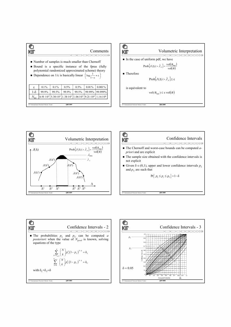
Confidence Intervals

The Chernoff and worst-case bounds can be computed a-priori and are explicit

The sample size obtained with the confidence intervals isnot explicit

Given (0,1), upper and lower confidence intervals pL

and pU are such that

Pr 1 δL Up p p


Confidence Intervals - 2

The probabilities pL and pU can be computed aposteriori when the value of Ngood is known, solvingequations of the type

with L+U

0

1 δ

1 δ

good

good

NN kk

L L Lk N

NN kk

U U Uk

Np p

k

Np p

k


Confidence Intervals - 3

ˆNR

Up

Lp


Bounds on the Binomial Distribution


Bounds on the Binomial Distribution

The so-called probability of failure is studied in the

scenario approach and in statistical learning theory

(discussed later in the course)

This required bounding the binomial distribution

0

B( ,ε, ) ε 1 εm

N ii

i

NN m

i


Bounding the Binomial Distribution and Sample Complexity

Theorem[1]: Given , (0,1) and m 0, if

then

[1] T. Alamo, R. Tempo and A. Luque (2010)

1

1 1inf log log( )

ε 1 δa

aN m a

a

0

B( ,ε, ) ε 1 ε δm

N ii

i

NN m

i


Bounding the Binomial Distribution and Sample Complexity

Suboptimal value of a is the Euler number e

Sample complexity is given by

Sample complexity is linear in

- 1/ (not quadratic!)

- m

-

1 1log

ε 1 δ

eN m

e

1log

δ


Probabilistic Methods:Benefits and Drawbacks

Benefits Drawbacks

very general method with immediatepractical applications, for example inaircraft design and process control industry

the results obtained provide no“deterministic certificate” of propertysatisfaction, for example H-infinityperformance

specific sample generation methods havebeen developed (e.g. for norm bounded sets,hit-and-run for convex sets, particlefiltering, importance sampling, MCMC)

for recursive methods the number ofrequired experiments is generally notspecified a priori

sample size bounds are available for non-recursive methods

the method does not cover the entire samplespace, but only a finite subset of it

Monte Carlo methods are very effective indealing with the “curse of dimensionality”;the probability of error is bounded

crucial points of the safety region can bemissed, this may lead to erroneousconclusions


Probabilistic Sorting of Switched Systems


Sorting of Switched Systems

Consider Lyapunov equations

L(P, A) = (Ai)T P + P Ai for all i =1, 2, …, N

The objective is to sort these N Lyapunov equations

according to their degree of stability (decay rate) using

a common P > 0 previously computed

Motivations: Deciding which systems are more stable

than others is useful information for the controller


LVRA for Matrix Sorting

The sorting operation should be performed quickly

because we are switching between N = 22n systems

This requires finding a LVRA which provides a

matrix sorting for the N equations L(P)

Matrix version of RandQuickSort is developed[1]

Technical difficulty: The equations may be not

completely sortable because of sign indefiniteness

[1] H. Ishii, R. Tempo (2009)


RandQuickSort for Matrices

Variation on RandQuickSort for sorting N = 22n

Lyapunov equations

Construction of the set of matrices which are not

sortable at that stage of the tree

We build a trinary (instead of binary) tree


RQS for Matrices: Trinary Tree

We use randomization at each step of the (trinary) tree


RQS for Matrices: Results

If the Lyapunov equations are completely sortable,

then the expected running time is (the same of RQS)

O(N log (N))

If the Lyapunov equations are not completely sortable,

then additional comparisons should be performed

The worst case number of additional comparisons is

N(N-1)/2


Computational Complexity of RAs


Computational Complexity of RAs

RAs are efficient (polynomial-time) because

1. Random sample generation of i) can be performed

in polynomial-time

2. Cost associated with the evaluation of J(i)) for

fixed i) is polynomial-time

3. Sample size is polynomial in the problem size and

probabilistic levels and


1. Bounds on the Sample Size

Chernoff bound is independent on the size of B, on theuncertainty structure, on the pdf and on the number ofuncertainty blocks

It depends only on probabilistic accuracy andconfidence

Same comments can be made for other bounds (such

as Bernoulli)


2. Cost of Checking Stability

Consider a polynomial

To check left half plane stability we can use the Routhtest. The number of multiplications needed is

The number of divisions and additions is equal to thisnumber

We conclude that checking stability is O(n2)

odd for 4

1 even for

4

22

nn

nn

nnsasaaasp 10),(


3. Random Sample Generation

Random number generation (RNG): Linear and

nonlinear methods for uniform generation in [0,1) such

as Fibonacci, feedback shift register, BBS, MT, …

Non-uniform univariate random variables: Suitable

functional transformations (e.g., the inversion method)

Much harder problem: Multivariate generation of

samples of with given pdf and support B

.It can be resolved in polynomial-time


Choice of the Probability Distribution


Choice of the Probability Distribution - 1

The probability Prob{S}

depends on the underlying

pdf

It may vary between 0 and 1

depending on the pdf


Choice of the ProbabilityDistribution - 2

The bounds discussed are independent on the choiceof the distribution but for computing an estimate ofProb{J() } we need to know the distribution

Research has been done in order to find the worst-casedistribution in a certain class[1]

Uniform distribution is the worst-case if a certaintarget is convex and centrally symmetric

[1] B. R. Barmish and C. M. Lagoa (1997)


Choice of the ProbabilityDistribution - 3

Minimax properties of the uniform distribution have

been shown[1]

[1] E. W. Bai, R. Tempo and M. Fu (1998)


CHAPTER 4

Random Vector Generation

Keywords: Radial distributions, inversion method, generalizedGamma density, uniform distribution in norm balls


Random Sample Generation


True Random Number Generators

Hardware sources of trulystatistically random numbers

High-voltage reverse-biasedP-N semiconductor junctions

Reverse-biased Zener diodes

Radioactive Decay

Lava-rand

Mechanical systems

entropy key


Random Generation

(Pseudo) random number generation (RNG): Various

methods are available for generation in the interval [0,1)

Linear and nonlinear RNGs, Fibonacci, feedback shift

register, BBS, MT, …

Non-uniform univariate random variables: Suitable

functional transformations (e.g., the inversion method)

Multivariate random variables: Rejection and conditional

density methods


Non-uniform Distributions:The Inversion Method

A standard tool for univariate random variablegeneration is the inversion method

Let w R be a r.v. with uniform distribution in [0, 1].

Let F be a continuous distribution function on R withinverse

Then, the r.v. z = F-1(w) has distribution F

10,)(:inf)(1 yyxFxyF


Non-uniform Distributions:The Inversion Method

F

w(i)

z(i) F(w(i))


Change of Variables

Let x be a random variable with pdf fx(x)

Let y = g(x), g invertible, and let

The pdf of y is

This method also has multivariate extensions

d ( )( ) ( ( ))

dy x

h yf y f h y

y

1(·) (·)h g


Example: exponential density

The exponential density is defined as

If x is uniform on [0,1], is an exponential rv

We perform the change of variables

( ) e 0y

yf y y

e logy

x y x

logy x


Example: Power Transformation

If a random variable x 0 has pdf fx(x) the randomvariable y=x for > 0 has pdf

Weibull: A rv with Weibull density with parameter a>0

can be obtained from an exponential rv via powertransformation. In fact, if then has density

11 1/λλ

1( ) ( )

λy xf y y f y

1( ) 0aa y

aW y ay e y

xx e 1/ay x( ) ( )y af y W y


Multivariate Random Vector Generation


Parametric Uncertainty

We study parametric uncertainty q in ℓp norm balls

Objective: Sample generation in the ball

B {q : ||q||p 1}

We are interested in uniform

sample generation within B

-1 -0.8 -0.6 -0.4 -0.2 0 0.2 0.4 0.6 0.8 1-1

-0.8

-0.6

-0.4

-0.2

0

0.2

0.4

0.6

0.8

1step 3


ℓp Vector Norms

Recall the ℓp vector norm of xFn

and the ℓ vector norm

1/

1

|| || | | for [1, )pn

pp i

i

x x p

|| || max | |ii

x x


Rejection Methods

Goal: to generate uniform samples in a set B (e.g. a

norm ball)

Idea: If we have a “simpler" set Bd that contains B, we

can generate uniform samples in Bd, and then reject

those that fall outside B

The rejection rate of the method is

Note: generation in Bd should be easy, membership of

B should be efficiently checkable

dvol( )

vol( )η

BB


Rejection Methods

Bd

B Find a bounding set Bd

Generate points x(i) in Bd

Keep the points in B

and reject the others


Rejection Methods:Curse of Dimensionality

Rejection rate for generation of

uniform samples in the sphere

using an hypercube as bounding

set

We obtain

)12/()π/2()(η n n n

n=1 n=2 n=3 n=4 n=10 n=20 n=30

1 1.2732 1.9099 3.2423 401.54 4.·107 5· 1013

Bd

B


Hit and Run Methods

The H&R algorithm has been proposed by Turchin in1971 and independently later by Smith in 1984

It provides a way of generating approximately uniformpoints in a body via random walks

H&R is easy to implement and it works for any convexbody (and also for nonconvex sets)


Hit and Run

Bz(0)

z(1) z(2)

z(3)

z(4)

z(T) x

Start with z(0) in B

Generate a random

direction

Take a random point

on the segment

Repeat T times

…

Return x z


Properties of H&R

The properties of H&R have been studied in numerousworks by Lovász and co-authors

After the mixing time T, the distribution of points can beconsidered “practically uniform”

It has been shown that the mixing time dependspolynomially on the problem dimension


Objective

Developments of techniques not based on asymptotic

methods such as Metropolis (random walk), MCMC,

Hit-or-Miss, importance sampling, …

These techniques are based on the univariate

(Generalized) Gamma density

Assume that we generate N i.i.d samples according to the

Gamma density, then with algebraic transformations we

obtain N i.i.d multivariate samples within B


Multivariate Distributions:the Jacobian Rule

Let fx(x1,…,xn) be a continuous density on the support

, and let

be a one-to-one and onto mapping, so that the inverse

is well-defined

Let y = g(x), then

n RB

: , ng RB TT

1(·) (·)h g

( ) ( ( )) ( ),y xf y f h y J x y y T


Multivariate Distributions:the Jacobian Rule

The Jacobian of the transformation is defined as follows

1 2

1 1 1

1 2

2 2 2

1 2

( )

n

n

n

p p n

xx x

y y y

xx x

y y yJ x y

xx x

y y y

( )i i

j j

x h

y y

y


Gamma Density

A random variable x has (unilateral) Gamma densitywith parameters (a,b) if

where · is the Gamma function

1 /1( ) 0

( )a x b

x af x x e x

a b

We write x G(a,b)

There exist standard and efficient methods for randomgeneration according to G(a,b)

1 ξ

0

( ) ξ dξ 0xx e x


Generalized Gamma Density

A random variable has (unilateral) Generalized Gammadensity with parameters (a,c) if

-1 -( ) , 0( )

cca xx

cf x x e x

a

We write x Gg(a,c)


Generalized Gamma Density

11

G ,( )

pxg p

p

pp e

p=1p=2p=4p=10p=100


Comments

Using power transformation method, a random variablex ~ Gg(a,c) is simply obtained as

x =z1/c

where z ~ G(a,1)

Samples distributed according to a (univariate) bilateral

density x ~ fx(x) can be easily obtained from a

(univariate) unilateral density z ~ fz(z)

Take x = sz, where s is an independent random sign

with values +1 and -1 with equal probability


Joint Density

Let x=[x1,…,xn]T with components independentlydistributed according to the (bilateral) GeneralizedGamma density with parameters 1/p and p

The joint density of x is

|| ||

1

( ) 2 (1/ ) 2 (1/ )

p ppi

nnxx

x n ni

p pf x e e

p p


Example: Multivariate Laplace

Recall that (1)=1 Multivariate (bilateral) Laplace

density

is a Generalized Gammadensity with parameters 1 and 1

1

| |1( )

2

n

ii

x

x nf x e


Example: Multivariate Normal

Multivariate (bilateral) normal Nwith mean 0 and covariance

is a Generalized Gamma densitywith parameters 1/2 and 2

T/2( ) π n x xxf x e

2I


Uniform Multivariate Generation in B

Theorem

Let xi be random variables distributed according to the(bilateral) Generalized Gamma density

Let w[0,1] be a random variable uniformly distributed

Then the vector

is uniformly distributed in B

px pgi ,G~ 1

T1 ,,,1

n

p

xxxx

xwy n


Algorithm Vector Uniform Generation

Input: n, p

Output: uniform random sample y

• Generate n independent real scalars i ~Gg(1/p,p)

• Construct vector x of components xi=si i where si are randomsigns

• Generate w uniform in [0, 1]

• Return1/n

p

y wx

x


Uniform Random Generation in ℓ2 - Step 1

-4 -3 -2 -1 0 1 2 3 4-4

-3

-2

-1

0

1

2

3

4step 1

Generate n iid randomreal scalars:

Construct xRn ofcomponents

(si i.i.d. random signs)

ξ ~ G 1( / , )g p p

11

G ,( )

pxg p

p

pp e



-1 -0.8 -0.6 -0.4 -0.2 0 0.2 0.4 0.6 0.8 1-1

-0.8

-0.6

-0.4

-0.2

0

0.2

0.4

0.6

0.8

1step 2 Construct the

normalized vector

The vector z isuniformly distributedon the surface of thep-norm ball

p

xz

x‖ ‖


-1 -0.8 -0.6 -0.4 -0.2 0 0.2 0.4 0.6 0.8 1-1

-0.8

-0.6

-0.4

-0.2

0

0.2

0.4

0.6

0.8

1step 3

Generate w uniform in[0,1], and return

.

The vector y isuniformly distributedinside the p-norm ball.


1/ 1/

p

n ny wzwx

x


Uniform Random Generation in B for p=1

-1 -0.8 -0.6 -0.4 -0.2 0 0.2 0.4 0.6 0.8 1-1

-0.8

-0.6

-0.4

-0.2

0

0.2

0.4

0.6

0.8

1


Uniform Random Generation in B for p=0.7

-1 -0.8 -0.6 -0.4 -0.2 0 0.2 0.4 0.6 0.8 1-1

-0.8

-0.6

-0.4

-0.2

0

0.2

0.4

0.6

0.8

1


Uniform Random Generation in B for p=4

-1 -0.8 -0.6 -0.4 -0.2 0 0.2 0.4 0.6 0.8 1-1

-0.8

-0.6

-0.4

-0.2

0

0.2

0.4

0.6

0.8

1


T11 ηξ,,ηξ,21

nn

p

xx

xwy n

Uniform Multivariate Generation in B (Complex Case)

Theorem

Let i be a complex random variable uniformlydistributed on the unit circle and

Let w[0,1] be a random variable uniformly distributed

Then the vector

is uniformly distributed in the complex ball B

ppgi ,G~ξ 1


Generation of Stable Polynomials


Schur Stability

The n-th degree discrete-time monic polynomial

is Schur if all its roots lie in the unit circle

Schur region

p denotes both poly p(z) and coefficient vector

20 1 2( ) np s p p z p z z

: ( ) is SchurR nn p p zS

0 1 1 R T nnp p p p


Hurwitz Stability

The n-th degree continuous-time polynomial

is Hurwitz if all its roots lie in the LHP

Hurwitz region

p denotes both poly p(s) and coefficient vector

10 1

R T nnp p p p

1 : ( ) is HurwitzR nn p p sH

20 1 2( ) n

np s p p s p s p s


Uniform Generation in the Schur Region

The Schur region for monic polynomials is bounded

We are interested in results that provide uniformdistribution in Sn

p0

p1

S2


Naive Method: Rejection

Lemma[1] The Schur region Sn lies inside the convex hullof (n+1) vertex polys

Generate random convex combinations

and pick only Schur stable ones

uniformly distributed in the unit simplex

( ) ( 1) ( 1) , 0, , k n kkv z z z k n

[1] A. T. Fam (1989)

0

( , ) ( )

n

k kk

p z v z 0, 1k k


Rejection Rate

The rejection rate is

We need another method!


Schur-Cohn-Jury Criterion

Given a polynomial p(z), define the reverse-orderpolynomial

Schur-Cohn-Jury Criterion: The polynomial p(z) is Schurstable if and only if |p0|<1 and the polynomial

of degree n-1 is Schur

10( ) ( )[ ] z p z p p z

1 10 1 1( ) ( ) 1n n n

np z z z z pp z pp z


The Fam-Meditch Parameterization

FM recursion[1]: Any monic Schur polynomialp[n](z)=p(z) of degree n can be obtained via the recursion

The tk's are referred to as reflection coefficients or Fam-Meditch (FM) parameters

Sweeping t inside the unit cube [-1,1]n yields all monicSchur polys of degree up to n

[0]

[ 1] [ ] [ ]

( ) 1;

( ) ( ) ( )k k kk

p z

z z p z t p zp

| | 1, 0, , 1kt k n

[1] Fam and Meditch (1978)


Uniform FM (UFM) Method

Various pdf's for tk lead to different coefficientdistributions

There exists a one-to-one mapping

Easily compute the Jacobian of the transformation

Hence we determine what pdf should be adopted for thetk to obtain a uniform pdf over Sn

[ 1,1]nnpt S

p t


Uniform FM (UFM) Method

Lemma[1,2]: If t1 is uniform over (0,1) and, for k = 2,…,n,tk has pdf proportional to

then the coefficients of the polynomial constructed viaFM recursion are uniform over Sn

Hence, we determine what pdf should be adopted for thetk to obtain a uniform pdf over Sn

[1] Beadle and Djuric (1997)

[2] Andrieu and Doucet (1999)

1 1( ) ( ( 1) ) ( ) , 1kk k k k kJ t t J t J


Algorithm: Uniform Schur Polynomials

Input: n,

Output: uniform Schur stable polynomial p[n](z).

• set t1=1, J1=1 and p[0](z)=1

• for k=2 to n

• construct Jk (tk) as

• generate tk according to

• construct p[k] via FM recursion;

• end for

( ) ( )kt k k kf t J t

1( ) ( ( 1) ) ( )kk k k k kJ t t J t


Uniform Schur Polys


Uniform Schur Polys: Roots Distribution

Root distribution (5th order poly)


Harder: Both the coefficient and the root domains areunbounded: uniform generation does not make sense(uniform density not defined)

Way to go?

– bound the coefficients,

– generate uniformly

– use rejection

The probability of picking a Hurwitz poly quicklydecreases to zero as the degree grows[1]

[1] A. Nemirovski and B. T. Polyak (1994)

Hurwitz Polynomials


Hurwitz: Conformal Mapping Method

Use the conformal mapping

which maps the interior of the unit disc to the open lefthalf plane

Generate a Schur stable poly

Compute a Hurwitz polynomial as

1( ) ( 1)

1n s

p s s ps

1 0( ) [1, , , ]npp z p

1

1

zz

z


Hurwitz: Conformal Mapping Method

Root distribution (5th order poly)


CHAPTER 5

Matrix Sample Generation

Keywords: Singular value decomposition, spectral norm, Haar density, conditional density method, Selberg integral



How to generate efficiently uniform matrix samples?

Vector case is completely solved for the real and

complex case, for any p norm ball

Matrix case is solved for the real and complex case, for

any Hilbert-Schmidt p-norm (reduces to the vector case)

For 1 and -induced matrix norms, the problem reduces

to the vector case


Hilbert-Schmidt Matrix Norms

The Hilbert-Schmidt ℓp norm of a matrix XFn,m

and

For p=2 Hilbert-Schmidt norm corresponds to the

Frobenius matrix norm

1/

1 1

|| || | | for [1, )pn m

pp ik

i k

X X p

|| || max | |ikik

X X

2|| || Tr * || ||FX XX X


ℓp nduced Matrix Norms

The ℓp induced norm of a matrix XFn,m

||ξ|| 1||| ||| max || ξ ||

pp pX X


ℓ1 and ℓ nduced Matrix Norms

The ℓ1 induced norm of a matrix XFn,m

where z1, …, zm are the columns of X

The ℓ induced norm of a matrix XFn,m

where w1T, …, wn

T are the rows of X

1 11,...,

||| ||| max || ||ii m

X z

11,...,

||| ||| max || ||ii n

X w


ℓ2 Induced Norm (Spectral Norm)

For XFn,m the spectral norm is defined as

2||| ||| ( )X X



Matrix spectral (max singular value) norm does notreduce to vector case

Hard problem for the spectral norm: Specific theory isneeded providing very technical results


First Attempt: Rejection

Methods based on rejection of samples generated froman outer-bounding set fail due to dimensionality issues

Let

then

Uniform generation in BF and B is easy

,( ) C :F n n

Fn n B

,(1) C : 1n n

B

(1) ( ) (1) (1)F n B B B B

,(1) C : ( ) 1n n B


Rejection Rates

Let be the average number of samples that one needsto generate in the outer set, to find one sample in thegood set

n= 2 3 4 5 6 8 10

12 8,640 8.7e8 2e16 2e26 5e54 1e95

F 8 468 1.8e5 4e8 6e12 2e23 1e37


Singular Value Decomposition

Consider Fn,m, m n

Singular Value Decomposition

= U V*

where UFn,n and VFm,n have orthonormal columns,

and

= diag{1,,…,n}

where … > n > 0


ℓ2 Induced Norm (Spectral Norm)

For Fn,m the spectral norm is defined as

2||| ||| ( )


A Class of Matrix pdfs

Unitarily invariant densities: depend only on the s.v. of

Radial symmetric densities: depend only on norm of

Uniform distribution in B

is a special case of radial density

( ) ( )I f f F

( ) ( ( ))R f f F

( )f U B


The pdf of theSingular Values – Real Case

Theorem[1]: Let Rn,m. The following statements are equivalent

The pdf f is unitarily invariant

The joint pdf of U, and V is )()()(),,(,, VffUfVUf VUVU

1,

2 2

1 1

( ) :

( ) : ,[ ] 0

( ) ( )

TU

TV i

nm n

R k i kk i k n

f U U UU I

f V V V V I V

f f

U

U

[1] G. Calafiore, F. Dabbene and R. Tempo (2001)


Real Matrices

is a normalization constant

Proof of previous theorem is based on the computationof the Jacobian of the mapping between and its svdfactors U, V

Details are very technical

( 1)/2

( 1)/21 1

( 1) / 2 ( 1) / 2(8π)

2 1 1

n m n m

R n mk k m n

k k

k k

R


Uniform Matrices – Real Case

For particular case of uniform matrices

with … > n > 0

The value of KR is obtained using the Selberg Integral

1/2

0

(( 1) / 2)!π

(3 / 2 / 2) ( / 2 1) (( 1) / 2)

nn

Ri

m iK n

i i i m n

2 2

1 1

( )n

m nR k i k

k i k n

f K


The pdf of theSingular Values – Complex Case

Theorem[1]: Let Cn,m. The following statements are equivalent

The pdf f is unitarily invariant

The joint pdf of U, and V is ,Σ, ( , , ) ( ) ( ) ( )U V U Vf U V f U f f V

*

*1,

22 ( ) 1 2 2C

1 1

( ) :

( ) : ,[ ] 0

( ) ( )

U

V i

nm n

k i kk i k n

f U U UU I

f V V V V I V

f f

U

U

[1] G. Calafiore, F. Dabbene and R. Tempo (2001)


Complex Matrices

is a normalization constant

Proof of previous theorem is based on the computationof the Jacobian of the mapping between and its svdfactors U, V

1

2 π

( )!( )!

n mn

C n

k

n k m k

C


Uniform Matrices – Complex Case

Consider particular case of uniform matrices, and changeof variables xi=i

2 , with ordering condition removed

The value of Kx is obtained using the Selberg Integral

n

i nkiki

nmixx xxxKxf

1 1

2)()(

1

02 )1()1(

)1(!

1 n

ix nmii

imn

K


Outline of Sample Generation Method

For uniform its svd factors are independentlydistributed

1. Generate the samples of U and V (easy problem)

2. Generate the samples of (hard problem)

3. Build matrix sample =U VT


Generation of Haar Samples

Uniform distribution over orthogonal (or unitary) group

is known as the Haar invariant distribution

Fundamental property: If U is Haar, then QU has samedistribution as U, for any fixed orthogonal (unitary)matrix Q


Generation of Haar Samples

Haar matrix URn,n may be generated by means of QRdecomposition as follows1. X=randn(n,n)

2. [Q,R]=QR(X)

3. U=Q;

Complex case works similarly

Rectangular Haar matrices work similarly


Generation of the Singular Valuesfor Complex Matrices


Conditional Density Method - 1

Is a general method that reduces generation according to

one n-dimensional distribution to n one-dimensional

sample generation problems

Drawback: requires computation of marginal densities

This is a very hard problem in general because requires

computing multiple integrals


Conditional Densities Method - 2

Write as

where

and

),...,( 1 nx xxf

)|()|()(),...,( 11122111 nnnnx xxxfxxfxfxxf

)()(

)|(111

111

ii

iiiii xxf

xxfxxxf

1 1 1( ) ( ,..., ) d di i x n i nf x x f x x x x


Conditional Density Method - 3

A vector xRn with density fx(x) can be obtained

generating sequentially the xi for i=1,…,n

Each xi is generated independently according to theunivariate distribution

)|( 11 iii xxxf


Computing the Marginal Density: Complex Matrices - 1

Let

be a partial Vandermonde matrix

1 22 2 21 2 1 2

1 1 11 2

1 1 1

( ) ( ) ( )i

i i i

n n ni

x x x

x x x x x x

x x x

V X X X

1 1 1( ) ( ,..., ) d di i x n i nf x x f x x x x


Computing the Marginal Density:Complex Matrices - 2

The marginal density is equal to

Where M=R-1

Proof of result based on Dyson-Mehta Theorem

1( ,..., )x if x x

T1

1

( )!( ,..., )

im n

x i x i i kk

n if x x K M x

M

V V

1for , 1, ,

1rlR r l nr l m n


Dyson-Mehta Theorem

Dyson-Mehta Theorem: Let ZnRn,n be a symmetric matrix suchthat

1. [Zn]ij=(xi,xj)

2.

3.

where d is a suitable measure, and c is a constant. Then

where Zn-1 is the submatrix obtained from Zn removing the row

and column containing xn

ψ( , ) d ( )x x x c ψ( , )ψ( , ) d ( ) ψ( , )x y y z y x z

1det( ) d ( ) ( 1) det( )n n nZ x c n Z


Computing the Marginal Density:Complex Matrices - 3

Given x1, x2,…, xi-1, the marginal density is expressed asa polynomial in xi

The constants Ci and the coefficients bi are computed bymeans of appropriate recursions

We have efficient way to compute conditional densities

2( 1)

0

( )n

m n ki i i i k i

k

p x K x b x

)1(2

011 ),,|(

n

k

kik

nmiiiii xbxKxxxf


Generation of the Singular Valuesfor Real Matrices


Computing the Marginal Density: Real Matrices - 1

Use again the conditional method

Mathematical details are different from the complex case

We again obtain marginals in “closed form”


Computing the Marginal Density:Real Matrices - 2

The marginal density fi (1,…, i) may be computed as

where

and

1

2 212

1

( ) ( , , )Rn

iK m n

i i kk

f

1 1( , , ) | ( ) | d ( ) d ( )i

i i n n iDx x x x x V

10 1i nD x x

d ( ) dk k kx x x 12υ ( 1)m n


Computation of

Theorem:i(x1,…, xi) is equal to

where i=(+1)(n-1)

and

12

1 1 1

2T

1 1

( , , )( )

0det

( , , ) 0 0

Rin

i iiK

i

i i

x xM x

x

x x

V

V

T

( ) ( )for even

( ) 0

( ) ( ) ( ) ( )

( ) 0 0 for odd,

( ) 0 0

i i

i

i i i iT

iT

i

S x xn i

x

M x S x x F x

x n i

F x

X

X

X

X

11 2

11 122 2 1

( ) ( )jj k

i ij k x xjk i j i jj k j k

S x F x


The Marginal Densities


Polynomial-Time Algorithms

Polynomial-time algorithms for the recursive generationof the singular values are been developed

The algorithms require at each step only additions andmultiplications of polynomial matrices

Technical details are very complicated

Methods becomes ill-conditioned for large n (n > 20)

For large n uniform matrices concentrate on theboundary of the norm-ball


Sample Generation: Summary

The details are highly technical

Computation of the pdf of the singular values

Computation of the pdf of U,V (Haar distribution)

Conditional density method

Closed-form solution of a multiple integral

Dyson-Mehta Theorem

MATLABTM

codes are available


Open Problem

Sample generation in the H ball

ω|| ( ) || sup ( ( jω))s


Application 1: Stability of a Flexible Structure


Example: Flexible Structure - 1

Mass spring damper model

Real parametric uncertainty affecting stiffness and

damping

Complex unmodeled dynamics (nonparametric)

m1

l1

k1

m2

l2

k2

m3

l3

k3

m4

l4

k4

m5

l5

k5

l6

k6


Flexible Structure - 2

M- configuration for controlled system and study

robustness

q1, q2 R

np C4 ,4

B ={: () < 1}

BAsICsM 1)()(

np

62

61

00

00

00

Iq

Iq


Probabilistic Radius

For fixed , we let

For given p*[0,1] we define the probabilistic radius

Clearly

(ρ) Pr is stablep A B C

ρ( *) sup ρ : (ρ) *p p p

1ρ( *)

μp


Probability Degradation Function

0 .3 5 0 .4 0 .4 5 0 .5 0 .5 5 0 .6 0 .6 5 0 .7

0 .9 4

0 .9 5

0 .9 6

0 .9 7

0 .9 8

0 .9 9

1

1 .0 1

P ro b a b i lis ti c ra d ius

Es

tim

ate

d p

rob

ab

ility

de

gra

da

tio

n

1/μ 0.394


Application 2: Probabilistic StructuredReal Stability Radius


Structured Real Stability Radius

Let ARn,n be a stable matrix, and consider the perturbedmatrix

with B, C of appropriate dimensions

Given A, B, and C, the real stability radius is the size ofthe smallest destabilizing perturbation

( ) ,A A B C B


Probabilistic Stability Radius

We assume random, and estimate the probability ofstability as a function of the uncertainty radius

For given p*, the probabilistic real stability radius isdefined as

We estimate the probabilistic stability radius usingrandomized algorithms

* *ρ ( , ) sup ρ : (ρ)R A p p p

(ρ) Pr ( ) is stable, p A B


Numerical Example

We studied the example

ICB

A

9809.28238.11812.44435.10764.28445.2

7190.01026.09139.18681.03964.02169.1

6973.02107.04244.00580.06813.01946.0

8705.20364.13362.36874.11677.14202.1

2641.48212.22311.53962.24700.15667.3

3271.15852.18166.21021.19633.09319.0


Numerical Example - 2

Compute p() for [0.01 0.05] with two differentstructures:

composed by three 2x2 full real blocks

composed by a 4x4 and

Date post:	30-Jun-2018
Category:	Documents
Upload:	dinhhanh
View:	218 times
Download:	0 times

ICT International Doctoral School Randomized Algorithms...

Documents