Identification of Neutrons Using DigitizedWaveforms

Rasmus Kjær Høier

Thesis submitted for the degree of Master of ScienceProject duration: 18 months, 60 hp

Supervised by Kevin Fissum and Hanno Perrey

Department of PhysicsDivision of Nuclear Physics

May, 2019

Abstract

The advantages of performing neutron-tagging measurements using a waveform digitizerare explored. An existing analog setup consisting of modular crate electronics at theSource-Testing Facility at the Division of Nuclear Physics in Lund, Sweden has beendigitally replicated. Neutrons are detected using an organic liquid-scintillator detectorwhile the corresponding 4.44 MeV gamma-rays are detected using inorganic scintillationcrystals. The performance of the digitizer-based setup is compared to that of the modularanalog setup in terms of neutron and gamma-ray pulse-shape discrimination and time-of-flight. The results obtained using the digitizer-based approach are superior to thoseobtained using the modular analog approach in all aspects. The digitizer-based approachis then successfully employed both to distinguish between neutrons and gamma-rays viaa convolutional neural network and to relate neutron deposition energy to neutron kineticenergy via time-of-flight.

Acknowledgments

I would like to thank all the members of the Sonnig group for creating a friendly at-mosphere and providing helpful feedback. In particular I want to thank my supervisorsHanno and Kevin. You gave me the freedom to jump down rabbit holes and open upcans of worms, but always helped me to stay on track. I very much appreciate yourguidance and support throughout this project. Finally I want to thank my wife Cibele.This project would not have been possible without your patience and advice.

Contents

List of Figures iii

List of Tables v

1 Introduction 11.1 Motivation . . . . . . . . . . . . . . . . . . . . . . . . . . . . . . . . . . . 11.2 The Basics . . . . . . . . . . . . . . . . . . . . . . . . . . . . . . . . . . . 2

1.2.1 Neutron/Matter Interactions . . . . . . . . . . . . . . . . . . . . . 21.2.2 Sources of Free Neutrons . . . . . . . . . . . . . . . . . . . . . . . 31.2.3 Scintillation Detectors . . . . . . . . . . . . . . . . . . . . . . . . 4

Detecting Gamma-rays . . . . . . . . . . . . . . . . . . . . . . . . 4Detecting Neutrons . . . . . . . . . . . . . . . . . . . . . . . . . . 5Photomultiplier Tubes . . . . . . . . . . . . . . . . . . . . . . . . 5

1.2.4 Neutron/Gamma-Ray Discrimination . . . . . . . . . . . . . . . . 61.2.5 Neutron Time-of-Flight and Tagging . . . . . . . . . . . . . . . . 8

2 Method 112.1 Experimental Infrastructure . . . . . . . . . . . . . . . . . . . . . . . . . 11

2.1.1 Source-Testing Facility . . . . . . . . . . . . . . . . . . . . . . . . 112.1.2 The Aquarium . . . . . . . . . . . . . . . . . . . . . . . . . . . . 122.1.3 Radiation Sources . . . . . . . . . . . . . . . . . . . . . . . . . . . 122.1.4 Fast-Neutron and Gamma-Ray Detectors . . . . . . . . . . . . . . 13

2.2 Signal Processing . . . . . . . . . . . . . . . . . . . . . . . . . . . . . . . 142.2.1 Analog . . . . . . . . . . . . . . . . . . . . . . . . . . . . . . . . . 15

Constant-Fraction Discriminators . . . . . . . . . . . . . . . . . . 15Trigger Logic . . . . . . . . . . . . . . . . . . . . . . . . . . . . . 16Time-to-Digital Converters . . . . . . . . . . . . . . . . . . . . . . 17Charge-to-Digital Converters . . . . . . . . . . . . . . . . . . . . . 18Charge-Comparison Pulse-Shape Discrimination . . . . . . . . . . 19

2.2.2 Digital . . . . . . . . . . . . . . . . . . . . . . . . . . . . . . . . . 20Digitizer Specifications and Configuration . . . . . . . . . . . . . 20Time Stamping . . . . . . . . . . . . . . . . . . . . . . . . . . . . 22Data Selection . . . . . . . . . . . . . . . . . . . . . . . . . . . . . 22

i

Energy Calibration . . . . . . . . . . . . . . . . . . . . . . . . . . 26Charge-Comparison Pulse-Shape Discrimination . . . . . . . . . . 26

2.3 Convolutional Neural Network . . . . . . . . . . . . . . . . . . . . . . . . 272.3.1 Training Dataset . . . . . . . . . . . . . . . . . . . . . . . . . . . 282.3.2 How It Works . . . . . . . . . . . . . . . . . . . . . . . . . . . . . 282.3.3 Implementation of the Network . . . . . . . . . . . . . . . . . . . 312.3.4 Decision Study . . . . . . . . . . . . . . . . . . . . . . . . . . . . 32

3 Results 353.1 Data Sets . . . . . . . . . . . . . . . . . . . . . . . . . . . . . . . . . . . 35

3.1.1 Overview and Comparison . . . . . . . . . . . . . . . . . . . . . . 353.1.2 Livetime and Threshold Alignment . . . . . . . . . . . . . . . . . 35

Deposited Energy . . . . . . . . . . . . . . . . . . . . . . . . . . . 35Time-of-Flight Spectra . . . . . . . . . . . . . . . . . . . . . . . . 37

3.2 Analog Setup . . . . . . . . . . . . . . . . . . . . . . . . . . . . . . . . . 383.2.1 Neutron Tagging . . . . . . . . . . . . . . . . . . . . . . . . . . . 383.2.2 Pulse-Shape Discrimination . . . . . . . . . . . . . . . . . . . . . 39

3.3 Digital Setup . . . . . . . . . . . . . . . . . . . . . . . . . . . . . . . . . 413.3.1 Neutron Tagging . . . . . . . . . . . . . . . . . . . . . . . . . . . 413.3.2 Pulse-shape Discrimination . . . . . . . . . . . . . . . . . . . . . 42

3.4 Misclassification . . . . . . . . . . . . . . . . . . . . . . . . . . . . . . . . 463.5 Neutron Kinetic Energy and Energy Deposition . . . . . . . . . . . . . . 48

4 Closing Remarks 514.1 Summary . . . . . . . . . . . . . . . . . . . . . . . . . . . . . . . . . . . 514.2 Conclusions . . . . . . . . . . . . . . . . . . . . . . . . . . . . . . . . . . 514.3 Outlook . . . . . . . . . . . . . . . . . . . . . . . . . . . . . . . . . . . . 52

Bibliography 53

ii

List of Figures

1.1 Scintillation detector. . . . . . . . . . . . . . . . . . . . . . . . . . . . . . 61.2 PS sensitivity. . . . . . . . . . . . . . . . . . . . . . . . . . . . . . . . . . 61.3 PS versus QLG. . . . . . . . . . . . . . . . . . . . . . . . . . . . . . . . . 71.4 Illustration of the neutron-tagging setup. . . . . . . . . . . . . . . . . . . 81.5 Sketch of a time-of-flight spectrum. . . . . . . . . . . . . . . . . . . . . . 91.6 Reference neutron energy spectrum for a Pu/Be source. . . . . . . . . . . 10

2.1 The Source-Testing Facility. . . . . . . . . . . . . . . . . . . . . . . . . . 112.2 The Aquarium. . . . . . . . . . . . . . . . . . . . . . . . . . . . . . . . . 122.3 Photographs of the detectors. . . . . . . . . . . . . . . . . . . . . . . . . 132.4 Schematic of the experimental setup. . . . . . . . . . . . . . . . . . . . . 142.5 Data-acquisition systems. . . . . . . . . . . . . . . . . . . . . . . . . . . . 152.6 Time walk resulting from leading-edge triggering. . . . . . . . . . . . . . 162.7 CFD trigger principle. . . . . . . . . . . . . . . . . . . . . . . . . . . . . 162.8 TDC calibration spectrum. . . . . . . . . . . . . . . . . . . . . . . . . . . 172.9 QDC calibration of the analog setup. . . . . . . . . . . . . . . . . . . . . 192.10 Sampling rate. . . . . . . . . . . . . . . . . . . . . . . . . . . . . . . . . . 202.11 Relative timing for NE213 detector pulses of different amplitudes. . . . . 232.12 Digitized pulse-height spectrum from the NE213 detector. . . . . . . . . 232.13 Examples of rejected digitized events. . . . . . . . . . . . . . . . . . . . . 252.14 Energy calibration of the digital setup. . . . . . . . . . . . . . . . . . . . 272.15 Selection of training and validation data using ToF information. . . . . . 282.16 Convolution of a vector and a kernel. . . . . . . . . . . . . . . . . . . . . 292.17 Two-layer CNN. . . . . . . . . . . . . . . . . . . . . . . . . . . . . . . . . 302.18 The Max pooling principle. . . . . . . . . . . . . . . . . . . . . . . . . . . 312.19 Training and validation accuracy of the CNN. . . . . . . . . . . . . . . . 322.20 Pulses classified by the CNN with more than 95% confidence. . . . . . . 332.21 CNN decision study. . . . . . . . . . . . . . . . . . . . . . . . . . . . . . 34

3.1 Comparison of analog and digital spectra from the NE213 detector. . . . 363.2 Analog and digital ToF spectra. . . . . . . . . . . . . . . . . . . . . . . . 373.3 ToF spectrum, analog setup. . . . . . . . . . . . . . . . . . . . . . . . . . 383.4 Analog PS spectrum as a function of deposited energy. . . . . . . . . . . 403.5 PS FoM for the analog setup. . . . . . . . . . . . . . . . . . . . . . . . . 40

iii

3.6 PS vs. ToF for the analog setup. . . . . . . . . . . . . . . . . . . . . . . 413.7 ToF spectrum, digital setup. . . . . . . . . . . . . . . . . . . . . . . . . . 423.8 Digital PS discrimination as a function of deposited energy. . . . . . . . . 433.9 PS FoM for the digital setup. . . . . . . . . . . . . . . . . . . . . . . . . 443.10 PS vs. ToF for the digital setup. . . . . . . . . . . . . . . . . . . . . . . . 453.11 Filtered ToF spectra for misclassification studies. . . . . . . . . . . . . . 473.12 ToF plotted against energy deposition for the digital setup. . . . . . . . . 493.13 Deposited energy and neutron kinetic energy. . . . . . . . . . . . . . . . 49

iv

List of Tables

1.1 Neutron nomenclature as a function of energy. . . . . . . . . . . . . . . . 3

2.1 Analog energy-calibration data. . . . . . . . . . . . . . . . . . . . . . . . 182.2 Summary of problematic events. . . . . . . . . . . . . . . . . . . . . . . . 242.3 Digital energy-calibration data. . . . . . . . . . . . . . . . . . . . . . . . 262.4 Parameters essential to the CNN. . . . . . . . . . . . . . . . . . . . . . . 32

3.1 Overview of the analog and digital data sets. . . . . . . . . . . . . . . . . 353.2 CC FoM parameters for the analog setup. . . . . . . . . . . . . . . . . . 413.3 CC FoM parameters for the digital setup. . . . . . . . . . . . . . . . . . . 443.4 Overview of PSD misclassification studies. . . . . . . . . . . . . . . . . . 48

v

List of Abbreviations

CC Charge Comparison

CFD Constant-Fraction Discriminator

CNN Convolutional Neural Network

DAQ Data Acquisition

ESS European Spallation Source

FIFO Fan-In Fan-Out

FoM Figure-of-Merit

LG Long gate

NIM Nuclear Instrument Module

PMT Photomultiplier Tube

PS Pulse Shape

PSD Pulse-Shape Discrimination

QDC Charge-to-Digital Converter

SG Short gate

STF Source-Testing Facility

TDC Time-to-Digital Converter

ToF Time-of-Flight

VME Versa Module Europa

vi

Chapter 1

Introduction

1.1 Motivation

In the late 1960s, the Nuclear Instrument Module (NIM) standard for experimentalphysics electronics was established. The NIM standard specifies certain parameters,such as module dimensions and back-plane voltages, which make it possible to easilycombine electronics modules from different manufacturers into a single signal-processingsystem. These modules each perform specific tasks, such as enforce thresholds, copy orsum signals or perform logic operations. When combined, they can be used to processsignals from experiments in the analog domain. The modular design also makes it easyto assemble, disassemble and recombine the modules to perform a wide array of differentsignal processing tasks. This makes it possible to easily construct electronics for signalprocessing in nuclear-physics experiments without necessarily knowing all of the exactfunctional parameters of each component. Simply knowing the operation the componentis to perform is sufficient. Later, additional modularized electronics components whichallow for an interface to computers were introduced. For example, the Versa ModuleEuropa (VME) modules are a widely used format for digitizing various features of analoginput signals, such as charge or time differences. VME modules can be considered abridge between the analog and digital domains.

Today, a leap forward is being taken in the field of instrumentation electronics withthe adoption of fully digital signal-processing techniques. This step is possible due toa variety of factors. For example, storage prices of less than 0.5 SEK per GB make itfeasible to save much more information than ever before. Also, increases in computerprocessing power have made the detailed investigation of large data sets more practical.Further, the falling cost and increasing performance of digitizers, devices which digitallysample analog signals at up to GHz frequencies, is key. We are now positioned on thecusp of the truly digital domain.

Currently, a wide variety of detectors under development for the European SpallationSource (ESS) need to be characterized. In particular, the 3He crisis has made it nec-essary to invent new detector technologies with high pixel count and granularity. TheSource-Testing Facility (STF) at the Division of Nuclear Physics in Lund, Sweden, cur-

1

rently provides well-understood radioactive sources and a dedicated experimental setupfor detector characterization. The setup is quasi-digital employing various standard NIMmodules for analog signal processing with digitization of charge and timing informationperformed by VME modules. Although this setup does employ some digitization, it willbe referred to as the analog setup to distinguish it from a fully digitizer-based digitalsetup. Using the analog setup, most components must be painstakingly fine tuned fora particular detector setup by changing delays, gate lengths and thresholds in order tooptimize the performance. This is not a trivial task.

The motivation for the work performed in this thesis is to emulate the NIM/VMEbased detector-characterization data-acquisition setup currently employed at the STFwith a fully digital digitizer-based system. In doing so, a large number of NIM and VMEmodules which need to be individually tuned to the task at hand will be replaced bya single digitizer module. This will enable optimizations to be performed digitally andmake it possible to study the effects of various thresholds, delays and gate lengths on thesame data set offline. Furthermore, access to the digitized waveforms on a pulse-by-pulsebasis will make it possible for advanced pulse-shape discrimination (PSD) techniques tobe applied to the data.

Thus, the potential of using modern digitization techniques to complement an existinganalog setup will be evaluated by comparing the performance of a well-established analogsetup with that of a digitizer-based setup. A classical charge-comparison method will beemployed for analog/digital PSD benchmarking. Furthermore, fully digital PSD will beinvestigated using a convolutional neural network, a technique which is not available whenemploying an analog electronics setup.

1.2 The Basics

1.2.1 Neutron/Matter Interactions

Neutrons are subatomic particles which together with protons make up atomic nuclei.With a mass of 939.6 MeV/c2, the neutron is 1.293 MeV/c2 more massive than the pro-ton and 1839 times as massive as the electron. Free neutrons were first discovered byChadwick in 1932, and have since come to play an important role as probes of matter.This is due to the fact that they are uncharged particles. With zero net electric charge,neutrons are a relatively penetrating type of radiation, capable of moving through theelectric fields of charged particles unaffected. When not bound in a nucleus, a neutrondecays into a proton via beta decay. This process has a half-life of 10.2 minutes [1], whichmeans that neutrons have to be freed from nuclei at the location of the experiment thatwill use them.

Neutrons are often classified according to their energy, since in different energy ranges,they have different probabilities for interactions of different types. The classificationsshown in Table 1.1 are given by Krane [2]. Fast neutrons are of particular interestto this project. For fast neutrons, the dominating interactions with matter are elasticand inelastic scattering. In elastic scattering, the neutron generally transfers part of its

2

Name Energy

thermal 0.025 eVepithermal 1 eVslow 1 keVfast 0.1-10 MeV

Table 1.1: Neutron nomenclature as a function of energy.

kinetic energy to a nucleus which recoils from the collision in its ground state. In inelasticscattering, the recoiling nucleus is excited, and it later de-excites by emitting for examplea gamma-ray. Thermal neutrons have wavelengths on the order of 0.1 nm which makesthem useful for examining the structure of matter on an atomic scale. Thermal neutronsinteract predominantly via absorption. Here a nucleus absorbs a neutron resulting in adifferent isotope of the same element, usually in an excited state. De-excitation can occurvia the emission of for example a gamma-ray [3]. The probability for neutron absorptionis roughly inversely proportional to its velocity. This means that fast neutrons need tofirst be slowed down or moderated to thermal energies if they are to undergo neutronabsorption.

1.2.2 Sources of Free Neutrons

Free neutrons can be produced for experimental use in different ways. Large-scale pro-duction involves accelerator facilities or nuclear reactors. Spallation neutron sources suchas ESS will produce neutrons by directing a highly energetic beam of protons onto aneutron-rich target. The collision will cause the target nucleus to fragment in a pro-cess known as spallation releasing many neutrons. For example, in the case of a singleGeV proton hitting a lead nucleus, around 25 neutrons may be produced [4]. Spallationneutron sources produce higher instantaneous neutron rates than any other currentlyexisting man-made neutron source. Nuclear reactors produce large fluxes of neutronsthrough fission, and a neutron beamline can be created by constructing a penetrationin the shielding [2]. The fundamental difference between an accelerator-based neutronbeam and a reactor-based neutron beam is that the former is pulsed whereas the latter iscontinuous. In either case, with moderation and specialized instruments, neutron beamswith specific energies can be produced.

On a smaller scale, neutrons may be freed by radioactive sources. An actinide-Beryllium neutron source is a combination of an alpha particle emitting actinide anda Beryllium base. For example, the actinide 238Pu decays into 234U as follows:

238Pu → 234U′ + α (Q1 −∑

iEγi)

→ 234U + α(Q1).(1.1)

The reaction has a Q-value Q1=5.59 MeV, which is energy shared between the recoilnucleus and the alpha particle. Note that the 234U nucleus may be left in either an

3

excited state or in its ground state. If it is left in its ground state, then the alpha particlecan at most receive a kinetic energy of Q1. If instead the nucleus recoils in an excited state(labeled 234U′ above), then less energy will be available for the alpha particle. Dependingupon the excited state, one or multiple gamma-rays may be released as the recoiling 234Ude-excites. This cascade of gamma-rays is useful, see Sec. 1.2.5.

Subsequent to its production, the alpha particle may then strike a 9Be nucleus, pro-ducing 12C and a free neutron, as shown below:

α(Q1) + 9Be → 12C + n(Q1 +Q2) 35%

→ 12C∗ + n(Q1 +Q2 − E1) 55%

→ 12C∗∗ + n(Q1 +Q2 − E2) 15%.(1.2)

This reaction has a Q-value of Q2=5.70 MeV, which is shared between the recoilingcarbon nucleus and the neutron according to momentum conservation. Roughly 35% ofthe time, 12C is produced in its ground state and the neutron can at most obtain energyQ1 +Q2=11.29 MeV. Approximately 55% of the time, 12C recoils in its first excited stateand de-excites by emitting a 4.44 MeV gamma-ray. Thus, in the case of a neutron freedtogether with the production of 12C in its first excited state, the kinetic energy of theneutron will be limited to Q1 + Q2 − Eγ = 6.85 MeV. The gamma-ray emitted by thede-exciting 12C is useful, see Sec. 1.2.5. Around 15% of the time, 12C recoils in the secondexcited state [5].

1.2.3 Scintillation Detectors

Scintillators generate pulses of visible light when ionizing radiation interacts with them.They are particularly useful for detecting uncharged particles such as gamma-rays andneutrons. An important feature of scintillators is that they should not re-absorb the scin-tillation light they themselves produce. This may be achieved by doping the scintillator,to facilitate de-excitations via different metastable states. The light emitted from themetastable states is shifted in energy so that it can pass through the scintillator withoutre-absorption. The lifetime of different metastable states may be exploited to identifythe incident particle species, see Sec. 1.2.4.

Detecting Gamma-rays

Photons of different energies generate scintillation light through different interactions withatomic electrons. These interactions are the photoelectric effect, Compton scattering andpair production [2]. Photons of energies below 0.1 MeV generally interact with atomicelectrons via the photo-electric effect. In this process, the photon is absorbed by a boundelectron which is ejected from the atom with an energy equal to the difference betweenphoton energy and the binding energy of the electron. This electron continues to interactin the detector. Compton scattering is the dominating effect between 0.1 and 5 MeV.

4

Here, a gamma-ray is scattered by a bound electron, which in turn is excited or freedfrom the atom. The scattered photon, which has been degraded in energy, continuesto interact in the scintillator as does the recoiling electron. Pair production dominatesbeyond 5 MeV. Here, a gamma-ray of energy Eγ > 2me spontaneously converts into anelectron and a positron near a nucleus [2]. The electron and positron share any excessenergy, which is then deposited in the scintillator via continued interactions. When thepositron comes to rest, it annihilates with another electron resulting in two 0.511 MeVgamma-rays. These gamma-rays may continue to interact with the scintillator. Theymay even escape the detector.

Detecting Neutrons

For fast neutrons, scintillation light is mainly produced by charged recoils resulting fromelastic scattering. In this case, the neutron energy will decrease from E to E ′ accordingto:

E ′ = E

(1− 4mAmn cos2 θ

(mA +mn)2

), (1.3)

where mn and mA are the neutron and nucleus masses and θ is the angle between therecoiling nucleus and the initial path of the neutron. From Eq. 1.3, it can be seenthat neutrons generally give up a larger fraction of their energy when they scatter fromlighter nuclei. For this reason, scintillation detectors are typically 1H rich. The recoilingproton will then produce ionization in the scintillator as it deposits its energy, resultingin scintillation light.

Photomultiplier Tubes

A photomultiplier tube is a device used to convert scintillation photons into a currentpulse, see Fig. 1.1. The scintillation light produced by neutrons and gamma-rays in ascintillator is converted to electrons at the photocathode via the photoelectric effect. Thecharge produced in this manner is not sufficient to result in a particularly strong signal,so a photomultiplier tube is used to increase the total charge. This results in a currentpulse that is large enough to be processed.

The PMT is connected to a high voltage source which provides a potential differencebetween the photocathode and the anode. This potential difference is used to acceleratethe electrons towards the anode through a series of dynodes. Each time an electronstrikes a dynode, multiplication occurs. The magnitude of the multiplication depends onthe gain and the number of dynodes, but factors of more than 107 are achievable. Theadvantage of a PMT is that it makes it possible to amplify charges by several orders ofmagnitude and that information about the original scintillation photon count and timingis preserved because the amplification is linear [3].

5

Figure 1.1: Scintillation detector. The blue volume to the left is the scintillator, which iscoupled to a PMT via a photocathode (yellow). The grey curves represent the trajectoriesof the electrons and the black curves are the dynodes. The red pulse to the right is theresulting elecronic signal. Figure from Ref. [6].

1.2.4 Neutron/Gamma-Ray Discrimination

The metastable states of scintillators have associated average decay times. Furthermore,the probability of a metastable state being occupied depends on whether the incidentparticle is a gamma-ray or a neutron [2]. For some scintillators, the differences in decaytimes between different metastable states which are excited by different types of particlespecies are large. This means that the signals produced by neutrons (recoiling protons)and gamma-rays (recoiling electrons) have different time dependencies or shapes. This inturn makes it possible to discriminate between them based on the resulting pulse shape(PS). A scintillator which demonstrates PS sensitivity to different particle species is saidto have pulse-shape discrimination (PSD) capabilities.

Short gateLong gate

Am

plitu

de

Time

Figure 1.2: PS sensitivity. Typical shapes of neutron and gamma-ray pulses from adetector with PSD capabilities. The blue gamma-ray pulse is significantly shorter thanthe red neutron pulse. “Short gate” and “long gate” refer to integration times.

6

PS can be parameterized in many different ways. One common method is the chargecomparison (CC) method. Pulses are integrated over two different timescales, typicallyreferred to as “long gate” (LG) and “short gate” (SG). Typical neutron and gamma-raypulse shapes are illustrated in Fig. 1.2 along with corresponding LG and SG integrationwindows. PS may be parameterized as:

PS = 1− QSG + a

QLG + b, (1.4)

where QSG and QLG are the total integrated charges in the SG and LG integrationwindows, respectively while a and b are constants added to the charge integrals QLG andQSG in order to facilitate fine tuning of the energy dependence of the PS parameter. Withoptimal choices of a and b, the neutron and gamma-ray distributions can be linearized,such that they can be separated with a single cut on the PS parameter, see Fig. 1.3.

If a scintillator has PSD capabilities, then signals from recoiling protons will havesignificantly more slow scintillation components. This will result in more charge in thetail of the scintillation pulse and hence a larger PS value than for electrons/gamma-rays.A typical way of visualizing the PS as a function of deposited energy is shown in Fig. 1.3.The upper distribution corresponds to neutrons and the lower corresponds to gamma-rays. It will generally be harder to discriminate between the two distributions at lowerdeposited energies.

A drawback with using analog electronics is that the LG and SG integration windowsneed to be decided before any measurements are taken. This makes optimization ofthe gate lengths tedious and time consuming, as an incorrect choice of gate length mayrender a data set useless. It is anticipated that the digitizer-based approach will greatlystreamline this process, as gates can be optimized after the data have been collected.

Linearization

𝛄 𝛄

nn

a, b tuned

QLG

PS

QLG

PS

Figure 1.3: PS versus QLG. Left panel: the parameters a and b are both zero. Rightpanel: a and b have been tuned to achieve a linear separation between neutrons (upperband) and gamma-rays (lower band). A typical cut is marked with a dashed red line.

7

Neutron and Gamma-ray detector

Gamma-ray detector

L

n, 𝜸 𝜸

s

Source

Start Stop

Delay

Figure 1.4: Illustration of the neutron-tagging setup. The detector sensitive to bothneutrons and gamma-rays (green) is placed a distance L from the source (green). Thegamma-ray detector (yellow) is placed closer to the source at a distance s.

1.2.5 Neutron Time-of-Flight and Tagging

Time-of-flight (ToF) measurements offer a conceptually elegant way to determine theenergy of a particle based on a known distance and the corresponding flight time. Theflight time is generally measured using a start pulse and a stop pulse together with aprecision oscillator.

Recall that an actinide/Beryllium source produces neutrons and gamma-rays. Thegamma-rays come both from the de-excitation of the actinide (a cascade of low-energygamma-rays) which follow the alpha particle emission and from the de-excitation of the12C (a single 4.44 MeV gamma-ray). This single gamma-ray emitted in conjunction withthe neutron may be used to “tag” the neutron and either start or stop a ToF measure-ment. Further, the low-energy gamma-ray cascade may be used to calibrate the ToFmeasurements.

By placing a gamma-ray detector close to the actinide/Beryllium source and a neutron/gamma-ray detector further away, the time difference between any two particles detectedin the two detectors may be measured, see Fig. 1.4. Often signal delay will be applied tothe gamma-ray detector to let the neutron/gamma-ray detector provide the start signaleven though it is located further away from the source than the gamma-ray detector. InFig. 1.4, the distance from the center of the actinide/Beryllium source to the center ofthe neutron/gamma-ray detector is L. Due to the applied delay the measured flight timeT will be shorter for neutrons than for gamma-rays. By instead using

T ′ = −T, (1.5)

time ordering is restored, with neutrons having longer flight times than gamma-rays.Figure 1.5 (left panel) shows a histogram of uncalibrated flight times T ′. This spectrummay be calibrated by considering two coincidental low-energy cascade gamma-rays fromthe de-excitation of the actinide. One of these gamma-rays is detected by the neutronand gamma-ray sensitive detector, while the other is detected by the gamma-ray detector.Since the speed of the gamma-rays is c and the source-to-detector distances and delays are

8

Calibration

Coun

ts

T´ (ns) ToF (ns)

Coun

ts

Figure 1.5: Sketch of a time-of-flight spectrum. Left: Spectrum of uncalibrated flighttimes. The gamma-flash is shaded blue, the neutron bump is shaded red, and the randomcoincidences are shaded orange. Right: The spectrum has been calibrated to a ToFspectrum by shifting T obsγ to T expγ .

fixed, the time difference between the start and stop signals is also fixed. This constanttime difference is known as the gamma-flash, and serves as an absolute timing calibrationpoint for the flight-time measurement. This calibration may be carried out by shiftingthe observed location of the gamma-flash T obsγ to the expected location T expγ defined asL/c. The calibrated time-of-flight, ToF is given by:

ToF = T ′ − (T obsγ − T expγ ). (1.6)

This produces the calibrated ToF spectrum shown in the right panel of Fig. 1.5. Ifinstead a neutron is detected by the neutron and gamma-ray sensitive detector and a4.44 MeV gamma-ray is detected by the gamma-ray detector, the flight time will alwaysbe longer than for a pair of gamma-rays because the speed of the neutron will alwaysbe less than c. From the resulting ToF for the neutron, the kinetic energy Kn may bedetermined classically according to:

Kn =1

2mnv

2n =

1

2mn

(L

ToF

)2

, (1.7)

where mn and vn are the mass and the speed of the neutron, respectively. Thus knowledgeof the distance from the center of the actinide/Beryllium source to the center of theneutron/gamma-ray detector together with the location of T obsγ in the uncalibrated flight-time spectrum is all that is needed to determine the energy of a tagged neutron on anevent-by-event basis.

Figure 1.6 shows an example of a tagged neutron energy spectrum (grey) contrastedwith the entire neutron energy spectrum (red) measured for a Pu/Be source [7]. Informing this spectrum the mapping from neutron ToF to neutron kinetic energy presentedin Eq 1.7 has been applied. Although neutrons from a Pu/Be source can have up to∼11 MeV, the tagged-neutron spectrum ends at ∼6.5 MeV. This is because only theneutrons accompanied by a 4.44 MeV gamma-ray are tagged. The full Pu/Be neutron

9

energy spectrum contains four peaks, two of which are visible in the tagged neutronspectrum. The reason that the full spectrum does not extend to as low energies asthe tagged neutron spectrum may be that the tagged spectrum has employed a loweramplitude threshold.

Sherzinger

Figure 1.6: Reference neutron energy spectrum for a Pu/Be source. Grey: a tagged neu-tron energy spectrum. Red: Neutron energy spectrum. Figure from Scherzinger et al [7].

10

Chapter 2

Method

2.1 Experimental Infrastructure

2.1.1 Source-Testing Facility

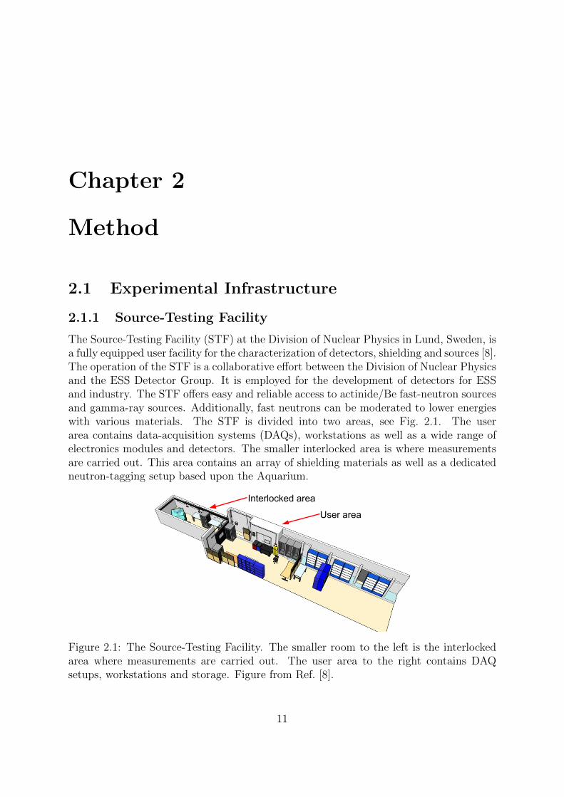
The Source-Testing Facility (STF) at the Division of Nuclear Physics in Lund, Sweden, isa fully equipped user facility for the characterization of detectors, shielding and sources [8].The operation of the STF is a collaborative effort between the Division of Nuclear Physicsand the ESS Detector Group. It is employed for the development of detectors for ESSand industry. The STF offers easy and reliable access to actinide/Be fast-neutron sourcesand gamma-ray sources. Additionally, fast neutrons can be moderated to lower energieswith various materials. The STF is divided into two areas, see Fig. 2.1. The userarea contains data-acquisition systems (DAQs), workstations as well as a wide range ofelectronics modules and detectors. The smaller interlocked area is where measurementsare carried out. This area contains an array of shielding materials as well as a dedicatedneutron-tagging setup based upon the Aquarium.

Interlocked area

User area

Figure 2.1: The Source-Testing Facility. The smaller room to the left is the interlockedarea where measurements are carried out. The user area to the right contains DAQsetups, workstations and storage. Figure from Ref. [8].

11

2.1.2 The Aquarium

The fast-neutron source may be located inside a 140×140×140 cm3 tank of water referredto as the Aquarium, see Fig. 2.2. The Aquarium has four horizontal cylindrical beamports intersecting at a central volume. A source and up to four gamma-ray detectors maybe placed within the central volume. The beam ports are air filled, allowing neutrons andgamma-rays to reach a neutron/gamma-ray detector placed next to the aquarium withoutpassing through shielding. Each of the beam ports can be plugged when not in use. Bymoderating and absorbing the fast neutrons, the water tank both provides shielding fromthe sources and gives rise to a distinguishable gamma-ray energy of 2.23 MeV produced inthe de-excitation of the deuteron via the 1H(n,γ)2H∗ reaction. This gamma-ray is usefulwhen performing energy calibrations, see Sec. 2.2.1 and Sec. 2.2.2. An actinide/Be sourcemay be positioned on the central vertical axis of the Aquarium and can be raised to thesame height as the ports for ToF measurements. In a “lowered” or “parked” position,there is no direct line-of-sight through air from the source through the ports. The fourdedicated gamma-ray detectors are located near the source, but are raised slightly toallow a direct line-of-sight from source through the ports, see Fig. 2.2.

Utilized gamma-ray detector

Neutron/gamma-ray Detector Pu/Be

source

140 cm

140 cm

L=114 cm

Unused gamma-ray detectors

Figure 2.2: The Aquarium. Left panel: Oblique view with the neutron/gamma-raydetector in front of one of the horizontal cylindrical beam ports. Lines-of-sight fromthe source out of two of the ports are indicated with arrows. The source and the fourgamma-ray detectors are located in the tubes at the center of the aquarium. Right panel:Top view with the source and detectors indicated by arrows.

2.1.3 Radiation Sources

Two radiation sources were used in this work. The actinide/Be fast-neutron and gamma-ray source 238Pu/9Be (referred to as Pu/Be) was used for tagging fast neutrons and forenergy calibration of the neutron/gamma-ray detector. As shown in Sec. 1.2.2, the Pu/Besource produces both a cascade of low-energy photons and fast neutrons, which ∼55%of the time are accompanied by the emission of a 4.44 MeV gamma-ray. The source hasbeen measured to produce approximately 2.99 · 106 neutrons per second [9]. The puregamma-ray source 60Co was used for detector calibration. 60Co decays to excited states of

12

60Ni via beta decay. De-excitation of 60Ni will result in gamma-rays of energies 1.17 MeVor 1.33 MeV [1].

2.1.4 Fast-Neutron and Gamma-Ray Detectors

As ToF depends on the accurate timing of γn and γγ pairs, it is essential to detect bothparticle species with accurate timing. In this work, two different detectors were used fordetecting neutrons and gamma-rays from the sources. Both of which produce pulses withnegative polarity. A liquid organic NE213 detector was used to detect both gamma-raysand neutrons while an inorganic Cerium-doped Yttrium Aluminum Perovskite crystal(YAP) detector was used to detect gamma-rays.

50.0 cm

12.5 cm

2 cm19.5 cm

Figure 2.3: Photographs of the detectors. Left: NE213 detector. Right: YAP detector.

Since its introduction in the early 1960s, the NE213 liquid organic scintillator has be-come the gold standard for fast-neutron detection due to its excellent neutron/gamma-raydiscrimination capabilities and high detection efficiency. The drawbacks of this scintilla-tor are that it is toxic and highly volatile with a flash point of 26◦C. The NE213 usedhere was produced by Nuclear Enterprises. It is equivalent to EJ301, currently producedby Eljen Technology [10]. The decay times of the first three scintillation components are3.16 ns, 32.3 ns and 270 ns [10]. It is contained in a 122×122×179 mm3 volume which isconnected to a photomultiplier tube via a lightguide1.

Near the source, four YAP detectors are placed. The YAP detectors are mounted onphotomultiplier tubes. These inorganic scintillators are largely insensitive to neutronsand provide excellent timing of gamma-rays. As the YAP detectors are located closer tothe source they experience a significantly higher gamma-ray flux than the NE213 detectordoes. This makes time resolution and decay time critical factors in their performance.The scintillation light has a decay time of ∼27 ns [12]. Howevever, it takes ∼100 ns forsignals to return to the original baseline level. This means that the detector can handlecount rates in the low MHz range without significant pileup. To simplify the analysisand limit the data rates, only one YAP detector was used in this project.

1This detector was constructed by Johan Sjogren as part of his thesis work in 2009-2010 [11].

13

2.2 Signal Processing

Two different experimental systems were employed. These experimental setups differedonly in the DAQ system used and shared the same physical setup of detectors, shieldingand radiation source. By sending the detector signals through an active splitter, bothDAQs could be run in parallel on the exact same detector signals. The first setup em-ployed NIM modules to process signals and generate a trigger decision. VME moduleswere used to digitize the timing and charge characteristics of the signals. The digitizeddata were transferred to a computer where they were saved and plotted in real time. Sincethis setup did most of the data processing via analog electronics, it will be referred toas the analog setup. The second setup was based on a digitizer which recorded detectorsignals as digital waveforms for offline analysis. Since all of the processing of the signalswas performed digitally, this setup will be referred to as the digital setup. Figure 2.5contrasts the analog and digital setups. The analog setup is composed of a variety ofNIM and VME modules as well as a large number of LEMO cables. The digital setup iscomposed of a single digitizer, which fits in a single VME slot. The digital setup is thusfar more compact spatially.

Analog setup

NE213 analog NE213 logic YAP analog Yap logic: Optical link

Digital setup

Delay

n, γ γ

QDC LG

NE213 PuBe

Latch

Computer

Digitizer

Fan-outYAPFan-out

CFD TDC

Computer

Start Stop1

4

2 3 CFD1

Fan-out

gates

QDC SG4

Figure 2.4: Schematic of the experimental setup. Green box: the digital setup. Yellowbox: the analog setup.

14

High voltage power supply

TDC and QDC modules

Analog signal processing

Digitizer

Figure 2.5: Data-acquisition systems. The analog DAQ rack is shown to the left. Digi-tization modules are highlighted by the orange arrow, and the power supply is indicatedby the blue arrow. A closeup of the analog electronics is shown in the red box. The singledigitizer module is shown highlighted in green to the right.

2.2.1 Analog

The detector signals were replicated by a fan-in-fan-out (FIFO) module and copies weresent to both the analog and the digital DAQ setups, see Fig. 2.4. On the analog side, thesignals were processed before time and energy information were sent through an opticallink to a computer running Centos 7.3 where it was written to hard drive.

Constant-Fraction Discriminators

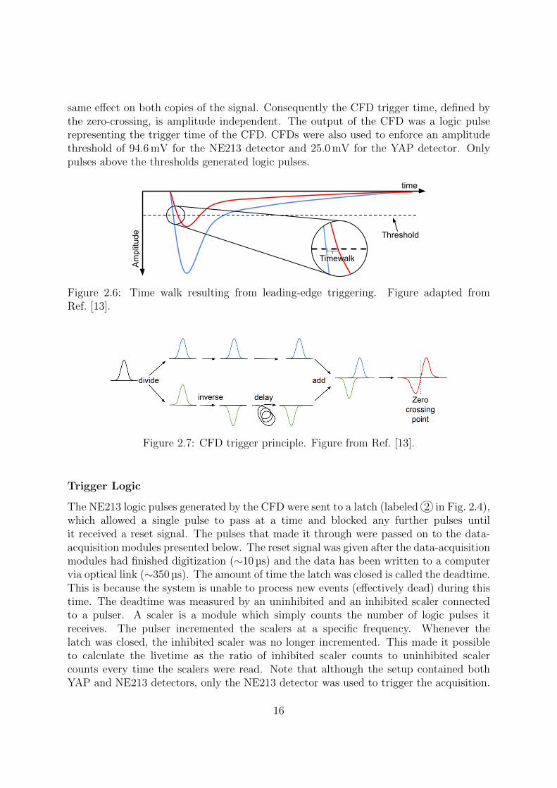
The YAP and NE213 pulses were sent to constant-fraction discriminators (CFDs), labeled1 in Fig. 2.4. CFDs were used because ToF measurements require precision timing of the

start and stop signals. Simply triggering on the leading edge of pulses will lead to “timewalk” for similarly shaped pulses of varying amplitudes. Time walk means that pulsesof the same shape but different amplitude will result in triggers at different times, seeFig. 2.6. As can be seen, the smaller pulse passes the threshold at a later time than thelarger pulse. By instead triggering on the point where a pulse reaches a certain fractionof its peak amplitude, time walk can nearly be eliminated [3]. This may be achieved bydividing or copying the signal, inverting one copy and delaying the other. The pulses arethen added and the zero crossing of the summed signal corresponds to a fraction of theinput pulse, see Fig. 2.7. Changing the amplitude of the incoming signal will have the

15

same effect on both copies of the signal. Consequently the CFD trigger time, defined bythe zero-crossing, is amplitude independent. The output of the CFD was a logic pulserepresenting the trigger time of the CFD. CFDs were also used to enforce an amplitudethreshold of 94.6 mV for the NE213 detector and 25.0 mV for the YAP detector. Onlypulses above the thresholds generated logic pulses.

time

Amplitude

Timewalk

Threshold

Figure 2.6: Time walk resulting from leading-edge triggering. Figure adapted fromRef. [13].

Figure 2.7: CFD trigger principle. Figure from Ref. [13].

Trigger Logic

The NE213 logic pulses generated by the CFD were sent to a latch (labeled 2 in Fig. 2.4),which allowed a single pulse to pass at a time and blocked any further pulses untilit received a reset signal. The pulses that made it through were passed on to the data-acquisition modules presented below. The reset signal was given after the data-acquisitionmodules had finished digitization (∼10 µs) and the data has been written to a computervia optical link (∼350 µs). The amount of time the latch was closed is called the deadtime.This is because the system is unable to process new events (effectively dead) during thistime. The deadtime was measured by an uninhibited and an inhibited scaler connectedto a pulser. A scaler is a module which simply counts the number of logic pulses itreceives. The pulser incremented the scalers at a specific frequency. Whenever thelatch was closed, the inhibited scaler was no longer incremented. This made it possibleto calculate the livetime as the ratio of inhibited scaler counts to uninhibited scalercounts every time the scalers were read. Note that although the setup contained bothYAP and NE213 detectors, only the NE213 detector was used to trigger the acquisition.

16

Since ToF measurements require both a start and stop signal, there can at most be asmany coincidences as there are pulses in the detector with the lowest count rate. TheNE213 detector experiences the lowest count rate. Thus, the deadtime was minimized bytriggering the acquisition on the NE213 detector.

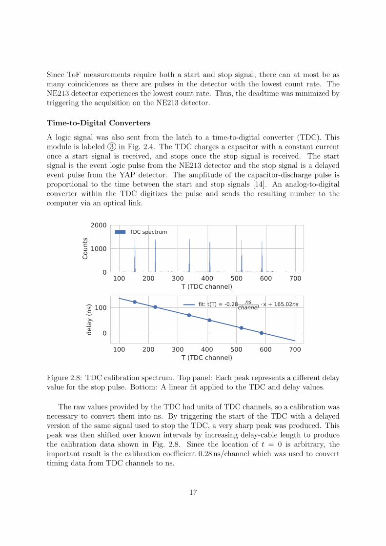
Time-to-Digital Converters

A logic signal was also sent from the latch to a time-to-digital converter (TDC). Thismodule is labeled 3 in Fig. 2.4. The TDC charges a capacitor with a constant currentonce a start signal is received, and stops once the stop signal is received. The startsignal is the event logic pulse from the NE213 detector and the stop signal is a delayedevent pulse from the YAP detector. The amplitude of the capacitor-discharge pulse isproportional to the time between the start and stop signals [14]. An analog-to-digitalconverter within the TDC digitizes the pulse and sends the resulting number to thecomputer via an optical link.

100 200 300 400 500 600 700T (TDC channel)

0

1000

2000

Coun

ts

TDC spectrum

100 200 300 400 500 600 700T (TDC channel)

0

100

dela

y (n

s) fit: t(T) = -0.28 nschannel x + 165.02ns

Figure 2.8: TDC calibration spectrum. Top panel: Each peak represents a different delayvalue for the stop pulse. Bottom: A linear fit applied to the TDC and delay values.

The raw values provided by the TDC had units of TDC channels, so a calibration wasnecessary to convert them into ns. By triggering the start of the TDC with a delayedversion of the same signal used to stop the TDC, a very sharp peak was produced. Thispeak was then shifted over known intervals by increasing delay-cable length to producethe calibration data shown in Fig. 2.8. Since the location of t = 0 is arbitrary, theimportant result is the calibration coefficient 0.28 ns/channel which was used to converttiming data from TDC channels to ns.

17

Charge-to-Digital Converters

The pulses that made it through the latch were used to generate 60 ns and 500 ns logicpulses with the first 25 ns preceding the CFD trigger point. These pulses acted as inte-gration “windows” or “gates” for the charge-to-digital converters (QDCs). In Fig. 2.4,these modules are labeled 4 . Copies of the analog current pulses were also sent to theQDC modules. Each module carried out an integration for the duration of the appliedgate. The resulting charges provided a measure of the energy deposited in the detectorby a given pulse on two different timescales. The QDC modules sent their outputs viaoptical link to a computer where they were written to the hard drive, see Fig. 2.4.

The charge integration performed by the QDC modules is a measure of the energydeposited in a detector. In the NE213 detector, neutrons interact primarily via scatteringfrom 1H while gamma-rays interact primarily with atomic electrons. It is customaryto calibrate a fast-neutron detector with gamma-ray sources, employing the “electron-equivalent energy”. Electron-equivalent energy corresponds to the amount of energydeposited by an electron. As gamma-rays interact with atomic electrons, they result inelectron-equivalent deposited energies. One way of performing this energy calibrationis the Knox method of examining the Compton edge corresponding to monoenergeticgamma-rays [15]. The maximum energy transferred by a gamma-ray to a recoil electronis given by:

(Ee)max =2E2

γ

me + 2Eγ[MeVee], (2.1)

where (Ee)max is the maximum energy transfered by a gamma-ray to a recoil electron, Eγis the energy of the gamma-ray and me is the mass of the electron. A Gaussian functionmay then fitted to the region of the Compton edge. The QDC channel where the Gaussiandistribution reaches 89% of its height is associated with (Ee)max. The 4.44 MeV Comptonedge produced by the de-excitation of 12C was used together with the 2.23 MeV Comptonedge produced by the de-excitation of 2H for calibration purposes.

Figure 2.9 shows a QDC calibration spectrum produced with a 500 ns integrationwindow. The narrow peak the furthest to the left in Fig. 2.9 is the pedestal. It is producedwhen the QDC is made to trigger when there is no current pulse in the detector. Thepedestal was produced for calibration purposes by allowing a small fraction of the YAPevents to trigger the DAQ. It represents the zero point of the QDC spectrum, so for theenergy calibration it is associated with 0 MeVee. All the values used in the calibrationare shown in Table 2.1.

QDC(channel) 67.5 1272.1 2718.9

E(MeV) 0 2.23 4.44(Ee)max(MeVee) 0 2.00 4.20

Table 2.1: Analog energy-calibration data. QDC channels fitted to known Comptonedges. See text for details.

The x-axis at the top of the panel shows the calibrated energy scale. The bump

18

immediately to the right of the pedestal is produced when the YAP trigger coincides bychance with a random deposition of energy in the NE213 detector. The 2.23 MeV and the4.44 MeV Compton edges have been highlighted in purple and orange. Using the pointslisted in Table 2.1, a linear calibration fit was made and plotted, see Fig. 2.9 (bottompanel). With this fit, the QDC spectrum was converted from channels to MeVee. It canbe seen that the uncertainty is greatest for the 2.23 MeV Compton edge.

Pedestal

Pedestal

Figure 2.9: QDC calibration of the analog setup. Top panel: Pu/Be spectrum measuredusing the NE213 detector. The upper x-axis has been calibrated. Bottom panel: Thecalibration fit produced with the Knox method. The pedestal is indicated with a red boxin both plots.

Charge-Comparison Pulse-Shape Discrimination

The CC method was implemented by integrating the pulses in the NE213 detector over aLG window of 500 ns and a SG window of 60 ns. As described in Sec. 1.2.4, the constants aand b were tuned to optimize the separation between the neutron and gamma-ray bands.

19

2.2.2 Digital

Digitizer Specifications and Configuration

A digitizer is an electronic device which converts analog signals to digital waveforms.A continuous analog signal is approximated by a list of numbers, each representing asingle sampling point, along with additional information such as a time stamp based ona global clock and the channel number of the signal. An acquisition is triggered when theamplitude of the input signal crosses a configurable threshold value. By this definition,a digitizer is similar to a digital oscilloscope. The main difference is that the oscilloscopehas a display and is optimized for portability and realtime diagnostic use, whereas thedigitizer is optimized for efficient high-rate data transmission to a computer where furtheranalysis can be carried out, either online or more commonly offline. The advantage ofa digitizer over a traditional analog DAQ system is that it allows the user to process asingle data set in multiple ways in order to optimize the parameters of the acquisition,without having to change anything in the physical setup or acquire subsequent data.The disadvantage is that the quality of the discretization of a continuous signal is limitedby the sampling rate, dynamic range, resolution and bandwidth of the digitizer as wellas the data-transfer rate of the read-out system. The sampling rate is the frequencyat which the digitizer samples a signal. The higher the sampling rate the better thedigital representation of the original analog signal, see Fig. 2.10. The dynamic rangeis the difference between the minimum and maximum voltage the digitizer can record.The resolution defines the number of partitions the dynamic range is divided into and istypically given in bits. The bandwidth determines which signals a digitizer can reproducewithout significant alteration. Signals whose Fourier expansion contain higher-frequencycomponents will require greater bandwidth2. The data-transfer rate defines how fast thedigitizer can transfer data to a computer. Low data-transfer rate will lead to greaterdeadtime.

0 25 50 75 100 125 150 175 200Time (ns)

1.0

0.5

0.0

U (a

rb. u

nits

)

analog signalf=f0f=f0/2

Figure 2.10: Sampling rate. Illustration of an analog signal sampled with two differentsampling rates, f0 and f0/2.

2For example, the perfect digitization of a square wave will require an infinite bandwidth, as itsFourier expansion is an infinite sum.

20

The digitizer used in this work is an 8 channel CAEN VX1751 waveform digitizer. Ithas a sampling rate of 1GS/s in standard mode, but can also be operated in double-edgesampling mode, which disables 4 cannels but increases the sampling rate to 2 GS/s [16].The data presented in this thesis were acquired in standard mode. This resulted inone data point per ns when digitizing signals. Given a set of sample points, there willalways be an infinite number of waveforms that fit the points [17]. This is called aliasing.Nyquist’s theorem states that if the sampling rate is at least twice as large as the highestfrequency component of the signal, aliasing may be avoided [17]. An even higher samplingrate is typically desirable. If the sampling rate is too low, important features such as peaklocation and amplitude will be less well defined, see Fig 2.10. In order to reproduce signalsaccurately, it is not enough to have a high sampling rate. The dynamic range, resolutionand bandwidth also need to be considered. The VX1751 digitizer has a 1 V dynamicrange, which means that the difference between maximum and minimum voltage is 1 V.This is controlled through the choice of signal polarity and baseline offset. The resolutionof the digitizer is 10 bits, so the 1 V dynamic range is divided into 1024 bins each ofsize 0.978 mV [16]. The VX1751 has a bandwidth of 500 MHz [16]. The bandwidth isimportant because it determines the frequency range of signals that can be digitizedwithout significant attenuation. If the frequency components as obtained from a Fourierexpansion of the signal are too high, then the amplitude recorded by the digitizer will belower than the actual amplitude of the input signal. A rule of thumb for evaluating thebandwidth needed by a given signal is:

B = 0.35/Trise, (2.2)

where Trise is the time it takes the pulse to rise from 10% to 90% of peak amplitudeand B is the bandwidth for which the signal is attenuated to only 70% of the originalamplitude [3]. Thus, with a 500 MHz bandwidth, the VX1751 will cause 70% attenuationin signals with 0.7 ns rise time. Since the signals studied here have rise times on the orderof 5−15 ns, bandwidth is not a limitation.

The digitizer was connected to a computer running Centos 7.4 via an optical link.This connection supports transfer rates of 80 MB/s [16]. However the number of eventstransfered at a time is also a limiting factor. In this work, the data were transferredon an event-by-event basis, which led to a significant reduction in livetime, see Chap. 3.The digitizer is controlled by WaveDump version 3.8.1 published by CAEN under theterms of the GNU General Public License [18]. It uses the proprietary digitizer controllibraries, also published by CAEN3. WaveDump configures the digitizer according to atext file supplied by the user. The number of data points per trigger is defined globallyfor all enabled channels. The signal polarity, trigger threshold and baseline offset alsoneed to be defined. The trigger threshold is the minimum amplitude relative to thebaseline that a pulse must have to be recorded. The baseline offset determines where inthe dynamic range of the digitizer the baseline is placed. A baseline offset of 0% will

3The version used in this work was modified to write all data to a single file rather than one file perchannel.

21

cause the entire range to be used for pulses of the selected polarity. This means thatundershoot will not be seen. Therefore it is best to use a small baseline offset. TheNE213 detector was connected to channel 0 of the digitizer and the YAP detector wasconnected to channel 1. Both the resulting NE213 and YAP pulses were of negativepolarity. An amplitude threshold of 48.8 mV was applied to the NE213 detector signalsand a threshold of 9.8 mV was applied to the YAP detector signals. A baseline offset of40% was inadvertently applied to the NE213 channel and a baseline offset of 10% wasapplied to the YAP channel. This meant that high amplitude NE213 pulses were clippedwhile high amplitude YAP pulses were not. The pulses thus saturated the dynamic rangeof the digitizer resulting in a small subset of large pulses with a flat top.

For a one hour run with the NE213 detector placed 1.05 m from the Pu/Be sourceand one YAP detector connected, data corresponded to ∼120 GB text file. The Pythonlibrary Dask was used for processing the data because it is optimized for processingdatasets that are too large to fit in random-access memory. It also runs on all availableprocessor cores [19]. After processing and data reduction, the data were saved to a binaryfile of size 7.3 GB . The Python library Pandas was used for additional processing andthe visualization of the reduced data set [20]4.

Time Stamping

The digital setup needs a method for providing a time stamp for each pulse from thedetectors. A global time stamp is provided by the digitizer for each acquired waveformor “event”. However, each event is 1204 ns long, and the pulses do not begin at theexact same point in time within the acquisition window. This is because the trigger clocktriggers on the leading edge of pulses and runs at only 125 MHz, whereas the sampling rateis 1 GHz. Consequently, it was necessary to precisely determine where in the samplingwindow the pulse was located. For this purpose, a software-based CFD algorithm wasimplemented. The algorithm searched the first 40 ns before the maximum amplitude ofthe pulse for the first sampling point to rise to 30% of the maximum amplitude. Linearinterpolation between this sampling point and the previous sampling point enabled a timestamp with resolution better than 1 ns to be generated. In Fig. 2.11, four pulses fromthe NE213 detector are plotted centered around their CFD trigger points. Although thistime stamp is given with sub-ns precision, the accuracy is limited by the determinationof the pulse amplitude, which in turn is limited by the sampling rate, resolution andbandwidth.

Data Selection

As the digitizer only enforced a threshold, additional selection criteria were applied offlineto filter the data set. Since the VX1751 triggered on all enabled channels simultaneously,all empty acquisition windows were discarded. This was done by determining and sub-tracting a baseline for each waveform. The baseline was determined by averaging over

4Python version 3.6.3 was used with Pandas version 0.23.4 and Dask version 1.0.0.

22

the first 20 ns of the waveform. The peak amplitude relative to this new baseline wasthen determined. An amplitude threshold of 24.4 mV was enforced removing all pulsesof amplitude below this value (negative polarity pulses).

During the digitizer configuration, a baseline offset that was too high was inadvertentlyapplied. This meant that only 60% of the dynamic range was available for signals fromthe NE213 detector. Events whose amplitude could not be contained in the availablerange had their peaks clipped. These 5.7% of the data were not discarded, but affectedthe QDC spectrum. The pulse-height spectrum shown in Fig. 2.12 highlights the clippedevents in green.

25 0 25 50 75 100 125 150t (ns)

250

200

150

100

50

0

mV

amplitude = 260 mVamplitude = 153 mVamplitude = 86 mVamplitude = 195 mVCFD trigger 30% of maximum amplitude

Figure 2.11: Relative timing for NE213 detector pulses of different amplitudes. A CFDalgorithm was used to generate a precise time stamp. A CFD trigger level of 30% of themaximum amplitude was used.

Clipped

Figure 2.12: Digitized pulse-height spectrum from the NE213 detector. Clipped eventswhich reached the limit of the dynamic range are highlighted in green.

23

Description Percentage of events Discarded

Pulses were clipped 5.7% NoUnstable baseline 2.7% YesCFD trigger in baseline determination window �0.1% YesCFD trigger too late for long-gate integration 1.1% YesCFD algorithm failed �0.1% Yes

Table 2.2: Summary of problematic events. In general the dataset was very healthy.

Certain events were removed because they caused either the baseline determination,pulse integration or CFD algorithm to produce spurious results. For example, in thecase of 2.7% of all events above trigger threshold, the baseline determination was deemedunsteady, see Fig. 2.13 (a). Events were removed when the standard deviation of samplesin the baseline-determination window was greater than 2 mV. A subset of the times thishappened was because a pulse was located inside the baseline-determination window asshown in Fig. 2.13 (b). This was identified when the CFD trigger point was located withinthe first 20 ns and happened 0.0016% of the time. Figure 2.13 (c) shows a situation wherethe CFD triggered so late in the acquisition window that not enough samples followedto carry out the 500 ns LG integration. This occurred in 1.1% of the events. And finally,0.00066% of the events were filtered because a peak was immediately preceded by asmaller peak, see Fig. 2.13 (d). Since the CFD algorithm searched the 40 ns immediatelyprior to the peak amplitude, it may have triggered due to the preceeding smaller pulse.All of the identified types of problematic events are summarized in Table 2.2.

24

Figure 2.13: Examples of rejected digitized events. Regions-of-interest are highlightedwith red boxes. (a) The baseline was deemed unstable. (b) A pulse was located insidethe baseline-determination window (a subset of (a)). (c) Less than 500 ns follow the CFDtrigger point, so the LG integration could not be carried out. (d) Closely adjacent pulsescaused the CFD algorithm to fail.

25

Energy Calibration

The energy calibration of the digital setup was carried out in a manner similar to theanalog setup, using the Knox method. The pulses were integrated digitally over theexact same gate lengths used in the analog setup, namely 60 and 500 ns starting 25 nsbefore the CFD trigger. A major difference compared to the analog setup was in thebaseline determination. For the analog setup, the pedestal was needed by the energycalibration to account for and subtract any baseline offset. It acted as a global baselinesubtraction. This was not necessary in the digital setup since the baseline was subtractedon an event-by-event basis during the initial data processing.

Both the Compton edges corresponding to 2.23 MeV and 4.44 MeV gamma-rays pro-duced by the Pu/Be source as well as a Compton edge corresponding to 1.33 MeV gamma-rays from a 60Co source were used for the calibration. The calibration points are listedin Table 2.3. In Fig. 2.14, the Compton edges corresponding to 1.33 MeV, 2.23 MeVand 4.44 MeV gamma rays are marked in red, purple and orange respectively. The 60Cosource produces gamma-rays of 1.17 MeV and 1.33 MeV, but due to energy resolutiononly the Compton edge corresponding to 1.33 MeV is visible. As with the analog setupthe uncertainty is the greatest for the 2.23 MeV Compton edge. The baseline shift on the

channel (mV·ns) 3791.4 7079.6 15480.9

Eγ (MeV) 1.33 2.23 4.44(Ee)max (MeVee) 0.96 2.00 4.20

Table 2.3: Digital energy-calibration data. Digitizer pulse integration channels fitted toknown Compton edges. See text for details.

NE213 channel offset was set too high, restricting the range available to negative pulsesto only 0.6 V. This affected the Compton edge of the 4.44 MeV gamma-ray. In spite ofthis problem, Fig. 2.14 shows that the calibration points still follow a linear trend withinuncertainty. The fit parameters were used to produce the calibrated x-axis in the upperpanel.

Charge-Comparison Pulse-Shape Discrimination

The CC method was implemented in the digital setup by integrating the waveforms over60 ns and 500 ns gates respectively, starting 25 ns before the CFD trigger. The exactsame gate lengths and timing employed by the analog setup were used here to facilitatea direct comparison of the two setups. In addition, the separation between neutron andgamma-ray distributions was linearized by fine tuning the parameters a and b as shownin Fig 1.3.

26

0 5000 10000 15000 20000 25000Digitizer pulse integration channel

10 1

100

101

102

103

104

105

Coun

ts

1.33 MeV2.23 MeV4.44 MeV238Pu/9Be60Co

0 5000 10000 15000 20000 25000Digitizer pulse integration

0

2

4

6

8

E (M

eVee

)

fit: E(x) = 0.28 10 3 MeVeechannel x -0.09MeVee

1.33 MeV2.23 MeV4.44 MeV

0 1 2 3 4 5 6 7E (MeVee)

Figure 2.14: Energy calibration of the digital setup. The Compton edges correspondingto the 1.33 MeV gamma-ray from 60Co and the 2.23 MeV and 4.44 MeV gamma-rays fromthe Pu/Be source have been used to perform the energy calibration.

2.3 Convolutional Neural Network

The biggest advantage a digitizer offers is that it records the entire pulse rather than justextracting a few parameters from it. With the entire waveform available, PSD can beapproached in ways that are not feasible with analog electronics. One such approach isto apply an artificial neural network to the task of discriminating between neutrons andgamma-rays. Artificial neural networks are function approximators which use learnedparameters called weights to perform a specified task. There are a variety of differentnetwork types. For image classification tasks such as PSD, convolutional neural networks(CNNs) set the gold standard. Training neural networks to perform neutron/gamma-rayPSD is not a new approach. It has been successfully implemented in a number of studiesfor various scintillators, see Ref. [21]. The key difference between what has previouslybeen done and what is done within this thesis lies in the manner the training data wereselected.

27

2.3.1 Training Dataset

To train a network to discriminate between neutrons and gamma-rays, a set of digitizedwaveforms along with labels defining the species of each waveform is needed. One ap-proach would be to create a precise simulation and train the network on the simulateddata. Then the labels are known with certainty to represent the waveforms to which theyare assigned. On the other hand, the simulated data must be an excellent representationof actual detector signals. This also implies that new simulations will be needed for newdetectors. Another approach is to use different PSD techniques for labeling data as eitherneutrons or gamma-rays. This is the approach taken by Griffiths et al. [21]. They labeltheir training data by plotting the number of samples within a given pulse that surpassesa certain threshold as a function of peak amplitude, and then making a cut to separateneutrons from gamma-rays. This approach is effective as long as the model used to gen-erate the training data is not systematically mislabeling a certain type of pulses, such aspulses in a certain energy range.

The approach taken here has been to take advantage of the extra information givenby the ToF spectrum. The ToF spectrum provides access to a labeled set of neutron andgamma-ray pulses in the form of the neutron bump and the gamma-flash, see Fig 2.15.The downside of this approach is that the ToF spectrum will also contain random coinci-dences, which means that the training data will contain some neutrons mistakenly labeledas gamma-rays and vice versa. Since the background is composed of random coincidencesand makes up only a small amount of the total training data, it is anticipated that thefalse neutrons/gamma-rays will not cause the network to systematically misclassify, butmerely slow down the training.

Samples[0,1,-1,-2,...][……………...][…………......][………...…...][…………......][………...…...][…………......]

…

Label1001011...

Labelled dataset

Figure 2.15: Selection of training and validation data using ToF information. Gamma-flash events are labeled 0 and events from the neutron bump are labeled 1.

2.3.2 How It Works

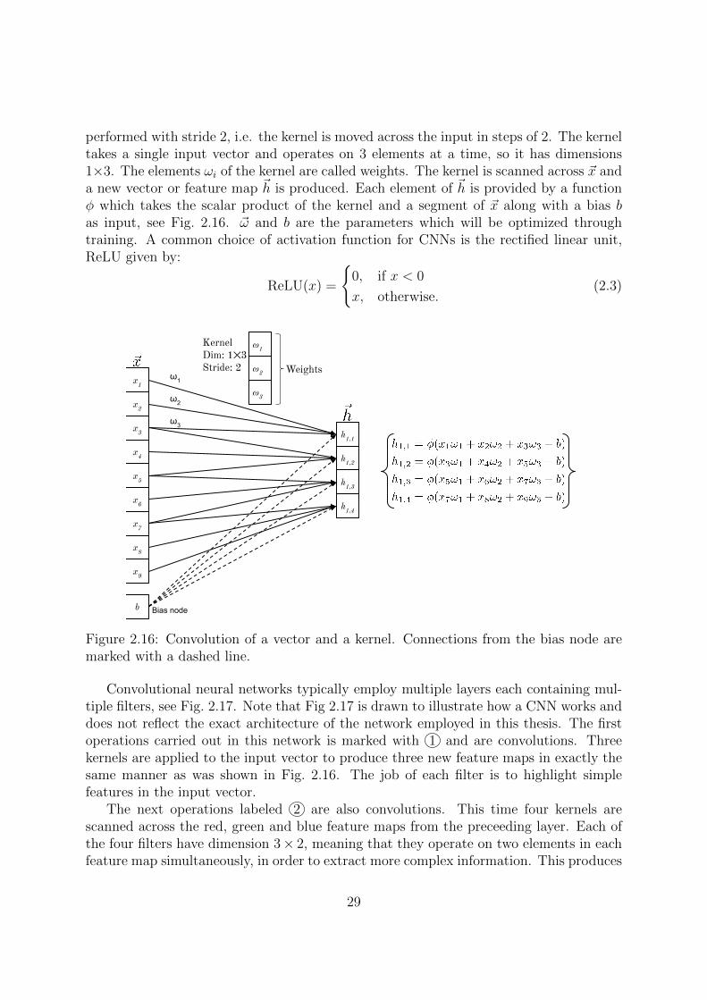
CNNs use kernels of weights to extract features from an input image. The essentialfeatures of a kernel are the size, the stride and the weights. Figure 2.16 shows an exampleof a kernel being applied to an input vector ~x. When applying the network to PSD, ~xwill be a digitized current pulse from the NE213 detector. In Fig. 2.16, the convolution is

28

performed with stride 2, i.e. the kernel is moved across the input in steps of 2. The kerneltakes a single input vector and operates on 3 elements at a time, so it has dimensions1×3. The elements ωi of the kernel are called weights. The kernel is scanned across ~x anda new vector or feature map ~h is produced. Each element of ~h is provided by a functionφ which takes the scalar product of the kernel and a segment of ~x along with a bias bas input, see Fig. 2.16. ~ω and b are the parameters which will be optimized throughtraining. A common choice of activation function for CNNs is the rectified linear unit,ReLU given by:

ReLU(x) =

{0, if x < 0

x, otherwise.(2.3)

x2

x3

x4

x5

x6

x7

x8

x9

KernelDim: 1⨉3Stride: 2

h1,1

h1,2

h1,3

h1,4

x1ω1

ω2

ω3

Weights

b Bias node

ω1

ω2

ω3

Figure 2.16: Convolution of a vector and a kernel. Connections from the bias node aremarked with a dashed line.

Convolutional neural networks typically employ multiple layers each containing mul-tiple filters, see Fig. 2.17. Note that Fig 2.17 is drawn to illustrate how a CNN works anddoes not reflect the exact architecture of the network employed in this thesis. The firstoperations carried out in this network is marked with 1 and are convolutions. Threekernels are applied to the input vector to produce three new feature maps in exactly thesame manner as was shown in Fig. 2.16. The job of each filter is to highlight simplefeatures in the input vector.

The next operations labeled 2 are also convolutions. This time four kernels arescanned across the red, green and blue feature maps from the preceeding layer. Each ofthe four filters have dimension 3× 2, meaning that they operate on two elements in eachfeature map simultaneously, in order to extract more complex information. This produces

29

the four new feature maps ~g1, ~g2, ~g3, ~g4. The next operation labeled 3 is a flattening ofthe four feature maps into a single vector ~f . In the final operation labeled 4 , the outputy of the network is given by an activation function φout, which takes a linear combinationof the elements of ~f as input. For binary classification problems, a common choice ofactivation function φout is the logistic function, which is bounded between 0 and 1:

φout(x) =1

1 + e−x. (2.4)

This function allows the output to be interpreted as a probability of the input waveform~x representing a neutron.

g4,1

g4,2g3,1

g3,2g2,1

g2,2

h3,1

h3,2

h3,3

h3,4

x2

x3

x4

x5

x6

x7

x8

x9

①ConvolutionUsing 3 kernels each withDimension: 1⨉3Stride: 2

x1

h2,1

h2,2

h2,3

h2,4

h1,1

h1,2

h1,3

h1,4

g1,1

g1,2

②ConvolutionUsing 4 kernels each withDimension: 3⨉2Stride: 2

f8f7f6

f5f4f3f2

f1

③Flattening all of the feature maps into a single vector

④Fully connected output layer

Input vector

Output neuron

f5f4f3f2

f1

Figure 2.17: Two-layer CNN. Each of the feature maps in the convolutional layers areproduced with a unique kernel, and has been given its own color. For readability, onlyconnections to the red and pink feature maps are shown. The other feature maps areconnected in the same manner. Bias nodes have also been omitted for readability.

The output of the network will be useless unless the weights have been properly trainedto extract relevant features. The network is trained through a simple yet incrediblypowerful method called “backpropagation”. In backpropagation, the derivative of anerror function with respect to each weight in the network is found through repeated useof the chain rule. These derivatives are then used to make adjustments to the weights inorder to minimize the error function. The error function used in this work is the binarycross-entropy error function. It is commonly applied to binary classification tasks and isgiven by:

E = − 1

N

N∑n

(dn log(y(~xn)) + (1− dn) log(1− y(~xn))) . (2.5)

This function calculates the average error E over N input vectors ~xn with labels dn. yn

30

is the output of the network. In the case of neutron/gamma-ray discrimination, eachvector ~xn will be a digitized waveform. If ~xn represents a neutron, then dn = 1 and thesecond term disappears. If instead ~xn represents a gamma-ray, then dn = 0 and the firstterm disappears. After propagating N waveforms through the network, the weights canbe updated using the derivatives of the error function. A simple updating method is thestochastic gradient descent updating rule:

ωt+1i = ωti − η

∂Et

∂ωi, (2.6)

where ωi is weight i in the network, E is the error function and t is the training iteration.The constant η is a scaling factor called the “learning rate”. It scales the correctionsdown to avoid overshooting optimal weights. The procedure is repeated until the errorfunction has converged at a minimum value.

2.3.3 Implementation of the Network

A CNN was implemented using Keras version 2.2.45 [22]. The main features of thechosen architecture are summarized in Table 2.4. In addition to convolutional layers, thisnetwork also contains “max pooling” layers. Max pooling layers reduce the size of eachfeature map individually by passing on only the maximum value of a given neighbourhoodof the input vector. With a size of 2 and stride of 2, input vectors are reduced to halftheir size, see Fig. 2.18. Due to the kernel size and stride as well as the max pooling,each node in the flattened layer is indirectly connected to a large number of samples inthe input layer. Both convolutional layers employ the ReLU activation function, whilethe final layer applies the logistic function.

23143

5

14

5

Max PoolingDimension: 1⨉2Stride: 2

Figure 2.18: The Max pooling principle.

The network was trained on events from the gamma-ray and neutron ToF peaks ofa 75 minute data set. This data-set was not used for any further analysis. 300 samples(or equivalently ns) from each pulse were used starting 20 ns prior to the CFD triggerpoint. 75% of the pulses or 3018 events from the neutron bump and 3018 events from thegamma-flash were used as labeled training data while the remaining 25% were used to

5Keras is a high-level framework for constructing deep-learning models in Python. It can be runusing different backends for carrying out operations on tensors. Here Tensorflow 1.12.0 was used asa backend.

31

Input layer: dimension 1×300Hidden layers Kernel Dimension N kernels Stride Activation functionConvolutional layer 9×1 10 4 ReLUMax pooling 2×1 - 2 -Convolutional layer 5×10 16 2 ReLUMax pooling 2×1 - 2 -

Fully connected: dimension 1× 144Output layer: dimension 1×1, activation function: φout(x) = 1

1+e−x .

Table 2.4: Parameters essential to the CNN.

0 25 50 75 100 125 150 175 200Epoch

0.7

0.8

0.9

Accu

racy

Training and validation accuracy

Training accuracyValidation accuracyEpoch = 53

Figure 2.19: Training and validation accuracy of the CNN. The dashed line indicates theepoch corresponding to the chosen model.

evaluate the model, see Fig. 2.19. Here the accuracy of the model, defined as the fractionof correctly labeled events, is plotted as a function of the epoch, with epoch defined asthe number of times the network has trained on the entire training dataset. The bluecurve shows the fraction of correctly labeled pulses achieved on the training data as afunction of iteration, while the red curve shows the same thing on the validation data.The red curve varies more since it represents a smaller dataset. As both training andvalidation data contain some fraction of incorrectly labeled background events, the modelis not expected to reach 100% accuracy on either data set. This plot shows that althoughthe performance on the training set keeps increasing, the performance on the validationset quickly levels out. For this reason, the model achieved at iteration 53 is used. Thenetwork is still learning beyond iteration 53, but it is no longer learning features thatgeneralize to the validation data. It is instead overfitting to noise in the training data.

2.3.4 Decision Study

One way to gain a deeper understanding of how the CNN distinguishes between neutronsand gamma-rays is to examine the pulses classified with a high level of confidence. Figure

32

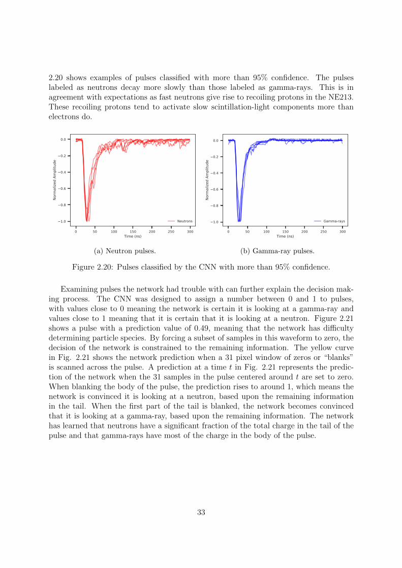
2.20 shows examples of pulses classified with more than 95% confidence. The pulseslabeled as neutrons decay more slowly than those labeled as gamma-rays. This is inagreement with expectations as fast neutrons give rise to recoiling protons in the NE213.These recoiling protons tend to activate slow scintillation-light components more thanelectrons do.

0 50 100 150 200 250 300Time (ns)

1.0

0.8

0.6

0.4

0.2

0.0

Norm

alize

d Am

plitu

de

Neutrons

(a) Neutron pulses.

0 50 100 150 200 250 300Time (ns)

1.0

0.8

0.6

0.4

0.2

0.0

Norm

alize

d Am

plitu

de

Gamma-rays

(b) Gamma-ray pulses.

Figure 2.20: Pulses classified by the CNN with more than 95% confidence.

Examining pulses the network had trouble with can further explain the decision mak-ing process. The CNN was designed to assign a number between 0 and 1 to pulses,with values close to 0 meaning the network is certain it is looking at a gamma-ray andvalues close to 1 meaning that it is certain that it is looking at a neutron. Figure 2.21shows a pulse with a prediction value of 0.49, meaning that the network has difficultydetermining particle species. By forcing a subset of samples in this waveform to zero, thedecision of the network is constrained to the remaining information. The yellow curvein Fig. 2.21 shows the network prediction when a 31 pixel window of zeros or “blanks”is scanned across the pulse. A prediction at a time t in Fig. 2.21 represents the predic-tion of the network when the 31 samples in the pulse centered around t are set to zero.When blanking the body of the pulse, the prediction rises to around 1, which means thenetwork is convinced it is looking at a neutron, based upon the remaining informationin the tail. When the first part of the tail is blanked, the network becomes convincedthat it is looking at a gamma-ray, based upon the remaining information. The networkhas learned that neutrons have a significant fraction of the total charge in the tail of thepulse and that gamma-rays have most of the charge in the body of the pulse.

33

0 20 40 60 80 100 120 140Time (ns)

1.2

1.0

0.8

0.6

0.4

0.2

0.0

0.2

Norm

alize

d am

plitu

de

Ambiguous pulse 0.2

0.0

0.2

0.4

0.6

0.8

1.0

1.2

Pred

ictio

nMasked pulse predictionOriginal prediction

Figure 2.21: CNN decision study. The green curve (left y-axis) shows a pulse the networkcould not clearly classify as either neutron or gamma-ray. The yellow curve (right y-axis)shows how the CNN prediction varies when part of the pulse is blanked.

34

Chapter 3

Results

3.1 Data Sets

3.1.1 Overview and Comparison

The data presented here were collected during a one-hour measurement with both theanalog and the digital setup running in parallel. A total of 4.3 million pulses from theNE213 detector were recorded by the analog setup. The digitizer saw 2.2 million pulsesfrom the NE213 detector over the same period of time. This large difference in countswas because the digital setup was configured to transfer each event individually, resultingin a very low livetime. In the analog setup, amplitude thresholds of 25.0 mV and 94.6mV were applied to the YAP detector and the NE213 detector, respectively. In thedigital setup, thresholds of 9.8 mV and 48.8 mV were applied to the YAP detector andthe NE213 detector, respectively. Having such a low threshold on the YAP detector wasfound to decrease the signal-to-noise ratio in the ToF spectrum, so a higher threshold of24.4 mV was applied offline in software. Table 3.1 presents an overview of the data sets.

SetupYAP

threshold (mV)NE213

threshold (mV)NE213

events (106)Livetime

%

Analog 25.0 94.6 4.3 44Digital 9.8/24.4* 48.8 2.2 **

Table 3.1: Overview of the analog and digital data sets. *An amplitude threshold of24.4 mV was enforced offline (see text for details). **The digital setup did not have amethod for determining livetime.

3.1.2 Livetime and Threshold Alignment

Deposited Energy

The analog and the digital setups were run with different amplitude thresholds. Toproperly compare them, a common threshold was necessary. Further, the analog and

35

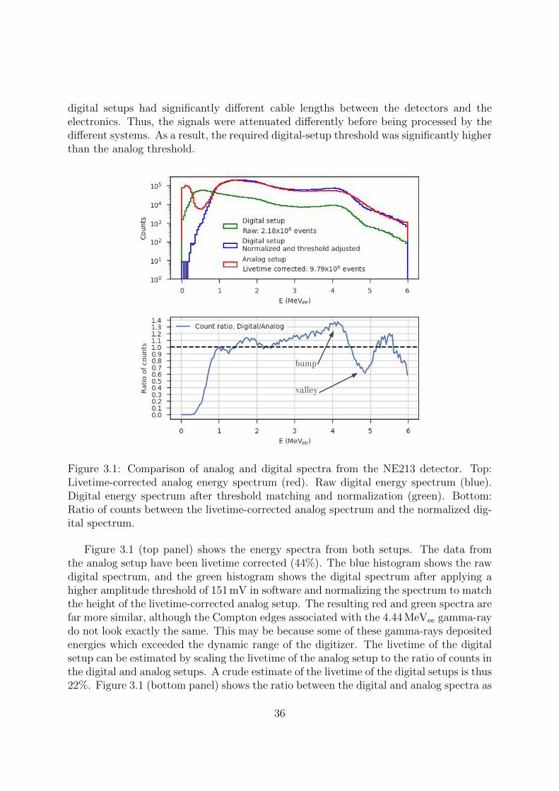
digital setups had significantly different cable lengths between the detectors and theelectronics. Thus, the signals were attenuated differently before being processed by thedifferent systems. As a result, the required digital-setup threshold was significantly higherthan the analog threshold.

bump

valley

Figure 3.1: Comparison of analog and digital spectra from the NE213 detector. Top:Livetime-corrected analog energy spectrum (red). Raw digital energy spectrum (blue).Digital energy spectrum after threshold matching and normalization (green). Bottom:Ratio of counts between the livetime-corrected analog spectrum and the normalized dig-ital spectrum.

Figure 3.1 (top panel) shows the energy spectra from both setups. The data fromthe analog setup have been livetime corrected (44%). The blue histogram shows the rawdigital spectrum, and the green histogram shows the digital spectrum after applying ahigher amplitude threshold of 151 mV in software and normalizing the spectrum to matchthe height of the livetime-corrected analog setup. The resulting red and green spectra arefar more similar, although the Compton edges associated with the 4.44 MeVee gamma-raydo not look exactly the same. This may be because some of these gamma-rays depositedenergies which exceeded the dynamic range of the digitizer. The livetime of the digitalsetup can be estimated by scaling the livetime of the analog setup to the ratio of counts inthe digital and analog setups. A crude estimate of the livetime of the digital setups is thus22%. Figure 3.1 (bottom panel) shows the ratio between the digital and analog spectra as

36

a function of deposited energy after both threshold alignment and normalization. Ideally,this ratio should be unity. This is not the case. Near the Compton edge correspondingto the 4.44 MeVee gamma-ray there is a bump and a valley. Again, this may be dueto the highest amplitude digitized pulses corresponding to the highest energy Comptonscattering events being clipped, causing them to register lower values of deposited energy.

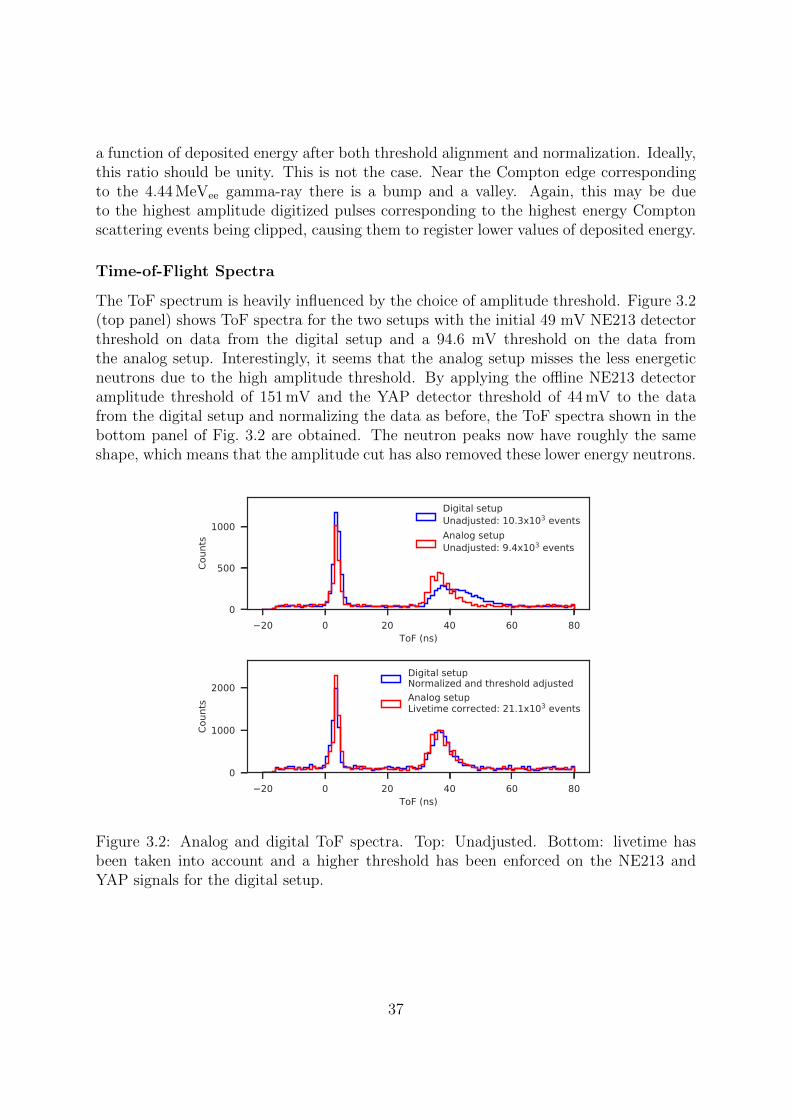
Time-of-Flight Spectra

The ToF spectrum is heavily influenced by the choice of amplitude threshold. Figure 3.2(top panel) shows ToF spectra for the two setups with the initial 49 mV NE213 detectorthreshold on data from the digital setup and a 94.6 mV threshold on the data fromthe analog setup. Interestingly, it seems that the analog setup misses the less energeticneutrons due to the high amplitude threshold. By applying the offline NE213 detectoramplitude threshold of 151 mV and the YAP detector threshold of 44 mV to the datafrom the digital setup and normalizing the data as before, the ToF spectra shown in thebottom panel of Fig. 3.2 are obtained. The neutron peaks now have roughly the sameshape, which means that the amplitude cut has also removed these lower energy neutrons.

20 0 20 40 60 80ToF (ns)

0

500

1000

Coun

ts

Digital setupUnadjusted: 10.3x103 eventsAnalog setupUnadjusted: 9.4x103 events

20 0 20 40 60 80ToF (ns)

0

1000

2000

Coun

ts

Digital setupNormalized and threshold adjustedAnalog setupLivetime corrected: 21.1x103 events

Figure 3.2: Analog and digital ToF spectra. Top: Unadjusted. Bottom: livetime hasbeen taken into account and a higher threshold has been enforced on the NE213 andYAP signals for the digital setup.

37

3.2 Analog Setup

3.2.1 Neutron Tagging

Figure 3.3 shows the ToF spectrum recorded by the analog setup. The neutron andgamma-ray peaks are indicated. In addition to these two peaks, there is an approximatelyflat background. This background represents uncorrelated particles triggering the TDCstart and stop, which is also why negative ToF values appear. The gamma-flash hasbeen shifted to be centered at 3.8 ns, the time it takes light to travel from the source tothe detector. The width of the gamma-flash is primarily due to the time resolution ofthe detectors. This depends on where in the detector volume the gamma-ray interacts.Secondary effects include signal attenuation in the cables, which might affect PS andthus rise time. This may in turn make the CFD less effective and may cause loss inthe time resolution. Furthermore, the final digitization by the TDCs may cause someloss of resolution. Differences in flight path between gamma-rays hitting the center ofthe NE213 detector and those that hit near the edge will be less than 1 cm, so thiswill not give rise to a substantial time spread. The neutron bump has more energetic

20 0 20 40 60 80 100 120ToF (ns)

0

200

400

600

800

1000

1200

Coun

ts

ToF spectrumAnalog setup

Neutrons

Gamma-rays

1 2 3 4 5 6 7Eneutron (MeV)

0

500

1000

Coun

ts

ScherzingerNeutrons

Figure 3.3: ToF spectrum, analog setup. The x-axis denotes the ToF from source toNE213 detector. The neutron and gamma-ray peaks are indicated with arrows. Thecoincidences highlighted in red have been converted to neutron kinetic energies and areshown in the upper right insert.

neutrons at lower ToF values and less energetic neutrons at higher ToF values. Since thedistance from the source to the detector is known, it is possible to convert the neutron

38

ToF into neutron kinetic energy. A range of 1.5−7 MeV was chosen. This correspondsto a time interval of 31−68 ns. The coincidences falling in this time interval have beenhighlighted in red in Fig. 3.3 and the corresponding energies are shown in the insert.The spectrum obtained by Scherzinger [7] (recall Fig. 1.6) has been superimposed. Thisspectrum has been normalized to produce the best qualitative agreement possible. TheScherzinger spectrum was measured with the same source but a different and smallerNE213 detector. That detector had only ∼10% of the scintillation volume of the oneused here and was cylindrical. Low-energy neutrons are clearly missing from the currentdata set, likely because a too large amplitude threshold has been applied. It also appearsthat the neutron-energy spectrum acquired by the analog setup is shifted to the right byroughly half an MeV. Below 2.5 MeV, the count rate in Fig. 3.3 increases. This is simplyan effect of the last ∼20 ns primarily consisting of background.

3.2.2 Pulse-Shape Discrimination

Neutrons and gamma-rays were discriminated using the PS parameter given in Eq. 1.4.The parameters a=120 QDC channels and b=0 QDC channels were found to linearize PSas a function of energy when gate lengths of 500 ns and 60 ns were used for the LG andSG integrations respectively. PS is shown as a function of deposited energy in Fig. 3.4.Pulses in the upper band (labeled neutrons) have a large amount of charge in the tailof the scintillation pulse. Pulses in the lower band (labeled gamma-rays) have a smalleramount charge in the tail of the scintillation pulse. This is confirmed by the presence ofthe Compton edges corresponding to 2.23 MeV and 4.44 MeV gamma-rays in the lowerband. The amplitude threshold of 94.6 mV gives rise to the sloping energy thresholdhighlighted with a red line in the figure. This is because pulses with higher PS have morecharge in the tail, so given two pulses of equal amplitude, the one with larger PS willcarry more charge.

The optimal PS-cut value of 0.259 was found by plotting a PS histogram and fittingGaussian functions to the neutron and gamma-ray distributions, see Fig. 3.5. The qualityof separation between the two distributions may be expressed as a Figure of Merit, FoM,defined in terms of the centers, C, of the Gaussian functions and their full width at halfmaximum, W :

FoM =Cn − CγWn +Wγ

(3.1)

Figure 3.5 shows histograms of the PS parameter along with the Gaussian fits used tocalculate the FoM. The corresponding parameters are listed in Table 3.2. The resultingintegrated FoM was 0.58, but was found to be highly energy-threshold dependent.

The neutron and gamma-ray distributions overlap at low deposited energies. Con-sequently, the PSD cut can result in misclassification. Orthogonal ToF information onparticle species can be used to quantify the extent of this misclassification. Figure 3.6shows PS plotted as a function of ToF, with neutron and gamma-ray distributions high-lighted. These distributions are not cleanly separated by the applied PSD cut. A signifi-cant amount of both neutrons and gamma-rays are mislabeled. Often the start and stop

39

Figure 3.4: Analog PS spectrum as a function of deposited energy. The dashed whiteline indicates the PSD cut. Structures due to the 2.23 MeV and 4.44 MeV gamma-raysare indicated. The red line indicates the amplitude threshold.

signal will be due to uncorrelated particles, rather than the previously discussed nγ andγγ pairs. These events are expected to form a flat background in the ToF spectrum dueto low rates. This may be seen in Fig. 3.3 at times longer than 50 ns. Since the eventsstill represent either neutrons or gamma-rays (ignoring the occasional muon), one wouldexpect them to be clearly separated into two bands in Fig. 3.6. This is not the case.

0.0 0.1 0.2 0.3 0.4 0.5PS

0

2000

4000

6000

8000

Coun

ts

FoM=0.58

NeutronsGamma-rays

Pulse shape histogramFit: W = 0.07, C =0.204Fit: Wn = 0.09, Cn=0.301

Figure 3.5: PS FoM for the analog setup.

40

FoM Cut Wγ Cγ Wn Cn

0.58 0.259 0.07 0.204 0.09 0.301

Table 3.2: CC FoM parameters for the analog setup.

0 20 40 60 80 100ToF (ns)

0.0

0.2

0.4

PS

--- Discrimination cut

NeutronsGamma-rays

100

101

Figure 3.6: PS vs. ToF for the analog setup. The dashed white line indicates the PSDcut. Note the logarithmic z-axis.

3.3 Digital Setup

3.3.1 Neutron Tagging

Fig. 3.7 shows the ToF spectrum acquired with the digital setup. No additional thresholdcuts or normalizations have been applied. Gamma-ray and neutron peaks are indicated.Random coincidences form a flat background. The width of the gamma-flash is againdue to the intrinsic time resolution of the detectors. A secondary effect may be thedigitization of the pulse. Limited resolution and sampling rate might cause the CFDalgorithm to trigger slightly too soon or too late. The red-shaded flight times in theneutron peak have been used to generate the energy spectrum shown in the insert ofFig. 3.7. The same time (31−68 ns) and energy (1.5−7 MeV) ranges used for the analogsetup have been used here. The spectrum has far more events at lower energies than thecorresponding spectrum for the analog setup, recall Fig. 3.3. This is because the digitalsetup had a lower amplitude threshold than the analog setup. Thus, neutrons with lessenergy, which generally produce current pulses of lower amplitude in the detector, maybe recorded by the digital setup. The energy spectrum looks qualitatively very similarto the superimposed reference spectrum of Scherzinger. However, the low-energy peak islocated at slightly higher energy. Scherzinger might have applied an even lower threshold.

41

20 0 20 40 60 80 100 120ToF (ns)

0

200

400

600

800

1000

1200

Coun

ts

ToF spectrumDigital setup

Neutrons

Gamma-rays

1 2 3 4 5 6 7Eneutron (MeV)

0

100

200

300

400

Coun

ts

ScherzingerNeutrons

Figure 3.7: ToF spectrum, digital setup. The x-axis denotes the ToF from source toNE213 detector. The neutron and gamma-ray peaks have been indicated with arrows.The coincidences highlighted in red have been converted to neutron kinetic energies andare shown in the upper right insert.

3.3.2 Pulse-shape Discrimination

As with the analog setup, 500 ns and 60 ns LG and SG integration windows were used toperform PSD. To linearize the bands, the parameters a and b from Eq. 1.4 were chosenas a=287 and b=120 (in uncalibrated digital-integration channels). The resulting PSDspectrum is shown in Fig. 3.8a. The Compton edges corresponding to 2.23 MeV and4.44 MeV gamma-rays are indicated with arrows. A large number of low-energy gamma-rays appear at the bottom left hand corner of the plot due to the lower threshold. A cutat PS=0.222 separates the neutron and gamma-ray bands. Again, the two distributionsoverlap at lower deposited energies.

The CNN described in Sec. 2.3 was also applied to the digitized waveforms. Thenetwork was trained to assign a value y between 0 (gamma-ray) and 1 (neutron) to eachsignal. The result is shown in Fig. 3.8b as a function of deposited energy. As for theCC method, the upper distribution corresponds to neutrons and the lower distributionto gamma-rays. The two bands are separated by a PSD cut at 0.5. To highlight that thedistributions overlap slightly at lower energies, the z-axis has been strongly suppressed.The CNN, trained on events from the two ToF peaks, allows for much cleaner separation

42

(a)

0 1 2 3 4 5 6 7E (MeVee)

0.0

0.2

0.4

0.6

0.8

1.0

CNN

pred

ictio

n

--- Discrimination cut NeutronsGamma-rays

2.23 MeV 4.44 MeV

0

200

400

600

800

1000

(b)

Figure 3.8: Digital PS discrimination as a function of deposited energy. The dashed whitelines indicate PSD cuts. Structures due to the 2.23 MeV and 4.44 MeV gamma-rays areindicated. Top panel: CC method. Amplitude threshold is indicated with a red line.Bottom panel: CNN method.

43

between particle species, so that the exact location of the PSD cut is much less criticalthan in either of the CC implementations.

As for the analog setup, a FoM was calculated based on Gaussian fits to the PSdistribution, see Fig. 3.9. The FoM parameters are summarized in Table 3.3. With anintegrated FoM of 0.78, the digital implementation of the CC method provides betterresults than the analog implementation.

FoM Cut Wγ Cγ Wn Cn

0.78 0.222 0.07 0.160 0.11 0.300

Table 3.3: CC FoM parameters for the digital setup.

0.0 0.1 0.2 0.3 0.4 0.5PS

0

2000

4000

6000

8000

Coun

ts

FoM=0.78

NeutronsGamma-rays

Pulse shape histogramFit: W = 0.07, C =0.160Fit: Wn = 0.11, Cn=0.300

Figure 3.9: PS FoM for the digital setup.

In Fig. 3.10, the digital CC and CNN predictions are shown as functions of ToF. Fig-ure 3.10a shows the narrow gamma-ray distribution and the wider neutron distribution asseparated by the digital CC method. The neutron and gamma-ray background forms twoslightly separated bands near prediction values 0.3 and 0.15 respectively. The two distri-butions overlap somewhat. In Fig. 3.10b, it can be seen that the CNN method providesa much better separation, although gamma-ray and neutron distributions still overlapslightly near prediction value 0.5. The distribution of random coincidences separates intoa gamma-ray band near prediction value 0 and a neutron band near 1.

44

0 20 40 60 80 100ToF (ns)

0.0

0.2

0.4

PS

--- Discrimination cut

NeutronsGamma-rays

100

101

(a)

0 20 40 60 80 100ToF (ns)

0.0

0.2

0.4

0.6

0.8

1.0

CNN

pred

ictio

n

--- Discrimination cut

Neutrons

Gamma-rays

100

101

(b)

Figure 3.10: PS vs. ToF for the digital setup. The dashed white line indicates the PSDcut. Note the logarithmic z-axis. Top panel: CC method. Bottom panel: CNN method.

45

3.4 Misclassification

Another way to compare the performance of the PSD methods is by estimating themisclassification. This can be done by evaluating the ToF spectrum in three differentregions and comparing the relative number of neutron and gamma-ray labeled events. Itis anticipated that the number of gamma-rays identified in a background region containingonly random coincidences should be the same as the number of gamma-rays identifiedin a chosen neighborhood of the neutron time-of-flight peak after scaling to the widthsof the regions. Likewise, the number of neutrons identified at the gamma-flash shouldcorrespond to the neutron-background expectation. The misclassification of gamma-raysand neutrons, Mγ and Mn respectively, can then be expressed as

Mγ(Rγ) =Nn(Rγ)− 〈Nn(Rγ)〉Ntotal(Rγ)− 〈Nn(Rγ)〉

(3.2)

Mn(Rn) =Nγ(Rn)− 〈Nγ(Rn)〉Ntotal(Rn)− 〈Nγ(Rn)〉

, (3.3)

where Nn and Nγ are the number of neutrons and gamma-rays identified in region R andNtotal is the sum of Nn and Nγ. 〈Nn〉 and 〈Nγ〉 are the expected numbers of neutrons andgamma-rays found by scaling the background rates to the width of R. This definition ofmisclassification relies on the assumption that the choice of limits for each of the threeregions does not seriously impact the results. The neutron peak neighborhood was setto match the range of neutron energies 1.5−7 MeV corresponding to 31−68 ns and thegamma-flash neighborhood was selected as 5 ns on either side of the gamma-flash center.It was found that as long as the peaks were contained in these regions the misclassificationschanged by at most ±0.5% for the digital setup and at most ±1% for the analog setup.

Figure 3.11 shows the ToF spectrum obtained with the analog setup filtered accordingto the CC method, as well as the ToF spectrum obtained from the digital setup filteredaccording to the CC and CNN methods. For each PSD implementation, gamma-raylabeled events are blue, neutron labeled events are red and their intersection purple.Ideally, the intersection of the distributions should be flat. However, if there is somesystematic misclassification, then the intersection will rise above the flat background levelin the ToF spectrum. This may be used to quantify the misclassification of a given PSDimplementation. For the analog setup, a high degree of contamination is evident in theform of the two purple bumps coinciding with the neutron and gamma-ray peaks. Thisgives an estimated misclassification of 16% for neutrons and 12% for gamma-rays. Thedigital setup provides less misclassification with the CC method, at 12% for neutronsand 3% for gamma-rays. The much higher misclassification for neutrons implies thatthe method is biased towards gamma-rays. The CNN approach reaches the best resultswith a gamma-ray misclassification of 4% and a neutron misclassification of 5%. Witha misclassification of nearly the same amount for both neutrons and gamma-rays, theCNN method does not appear to have a strong bias towards either particle species. Theneutron background is found to be nearly the same by the analog and digital CC methods,

46

25 0 25 50 75 100 125 150ToF (ns)

0

200

400

600

800

1000

1200Co

unts

Analog setupCC

n region: 16% mislabeled region: 12% mislabeled

Background region:37% neutronsAllGamma-raysNeutrons

(a) PSD cut at PS = 0.259.

25 0 25 50 75 100 125 150ToF (ns)

0

200

400

600

800

1000

1200

Coun

ts

Digital setupCC

n region: 12% mislabeled region: 3% mislabeled

Background region:38% neutronsAllGamma-raysNeutrons

(b) PSD cut at PS=0.222.

25 0 25 50 75 100 125 150ToF (ns)

0

200

400

600

800

1000

1200

Coun

ts

Digital setupCNN

n region: 5% mislabeled region: 4% mislabeled

Background region:45% neutronsAllGamma-raysNeutrons

(c) PSD cut at prediction = 0.5.

Figure 3.11: Filtered ToF spectra for misclassification studies.

47

at 37% and 38% respectively. The CNN method finds a significantly higher backgroundof neutron events at 45%. This together with the high misclassification rates for the CCmethods hints at them being biased towards gamma-rays. The results from all three PSDimplementations are summarized in Table 3.4.

γn-region(% misclassified)

γγ-region(% misclassified)

Background region(% neutrons)

CCAnalog

16 12 37

CCDigital

12 3 38

CNNDigital

5 4 45

Table 3.4: Overview of PSD misclassification studies.

3.5 Neutron Kinetic Energy and Energy Deposition

Figure 3.12 shows energy deposition in the NE213 detector as a function of ToF measuredwith the digital setup. The least energetic neutrons (ToF ∼60 ns) have a smaller spread indeposited energy, whereas the faster neutrons (ToF ∼35 ns) have a much larger spread.This may be explained by the fact that in the NE213 detector, the neutron scattersprimarily from 1H nuclei. Thus, by Eq. 1.3, the neutron may deposit up to its entirekinetic energy in a single scatter. A low-energy neutron simply has less energy to transfer,resulting in the smaller spread in deposited energy.

The scintillation-light output produced by an NE213 detector is given by [23]:

Edeposited = C(

0.83 · Ep − 2.82 ·(

1− e(−0.25·E0.93p )))

, (3.4)

where Edeposited and Ep is the energy deposited in the detector in MeVee and the kineticenergy of the proton producing the light in MeV, respectively. The parameter C is ascaling parameter which allows for such effects as scintillator aging and batch-to-batchvariation in scintillator quality. As a first approximation the kinetic energy found fromthe ToF may be used in place of proton energy. This is not a bad approximation whenusing a large detector where the neutron can undergo multiple scattering transferringmost of its energy to recoiling protons. In Fig. 3.13 (top panel), the deposited energyis shown for three intervals of kinetic energy of the neutron. Clearly, both the positionsand the widths of the peaks vary. The positions of the deposited-energy distributionsare plotted as a function of neutron kinetic energy in the bottom panel. Uncertaintiescorrespond to the fitted widths. By fitting Eq. 3.4 to these data, the value of C wasfound to be 0.62. This means that the NE213 scintillator is performing at 62% of thebenchmark. Note that Rofors measured this parameter for this detector in 2016 and

48

found it to be 86% [13]. The detector thus seems to be degrading at a rate of ∼8%per year. This is likely because the boroscilicate glass/photocathode interface needs newoptical grease.

0 20 40 60 80 100ToF (ns)

0

2

4

6

E (M

eVee

) Gamma-raysNeutrons

100

101

102

Figure 3.12: ToF plotted against energy deposition for the digital setup.

0 1 2 3 4 5 6Eneutron (MeV)

0

1

2

3

E dep

osite

d (M

eVee

)

Fit: C=0.62slice 0slice 5slice 10

0.0 0.5 1.0 1.5 2.0 2.5 3.0Edeposited (MeVee)

0

20

40

60

Coun

ts

slice 0: 2.15 MeVslice 5: 3.60 MeVslice 10: 5.06 MeV

Figure 3.13: Deposited energy and neutron kinetic energy. Top: Gaussian fits to de-posited energies for selected slices of neutron kinetic energy. Bottom panel: depositedenergy as a function of neutron kinetic energy, along with the fitted function.

49

50

Chapter 4

Closing Remarks

4.1 Summary

The advantages of performing neutron-tagging measurements using a waveform digitizerwere explored. An existing analog setup consisting of modular crate electronics at theSTF at the Division of Nuclear Physics in Lund, Sweden was digitally replicated. Neu-trons were detected using an organic liquid-scintillator detector while the corresponding4.44 MeV gamma-rays were detected using inorganic scintillation crystals. The perfor-mance of the digitizer-based setup was compared to that of the modular analog setup interms of neutron and gamma-ray PSD and ToF. The results obtained using the digitizer-based approach are superior to those obtained using the modular analog electronics ap-proach in all aspects. The digitizer-based approach was then succesfully employed toboth distinguish between neutrons and gamma-rays via a CNN and to relate neutrondeposition-energy to neutron kinetic energy via ToF.

4.2 Conclusions

In conclusion, the digital setup significantly outperformed the analog setup in terms of CCPSD capabilities. The digital setup also facilitated a CNN-based PSD approach, whichoutperformed both the analog and the digital CC implementations. The measurementsfrom the analog setup were hampered by the use of a too-high amplitude threshold.This is a classic pitfall associated with analog electronics. Unlike the digitizer approach,choices of thresholds and gate lengths for the analog setup can not be undone afterthe dataset has been acquired. A limiting factor with the digital setup is the dynamicrange, which needs to be carefully allocated. Likewise the data transfer needs to bepartitioned into blocks to minimize deadtime. Indeed, the dynamic range of the digitizerwas not optimized for the measurements performed here, resulting in clipping for highenergy gamma-rays. Additionally, ToF information was used to relate the neutron kineticenergy to its deposited energy. It was found that the NE213 detector had degraded withtime.

51

4.3 Outlook

Much has been learned about the two DAQs which can be used to make them perform evenbetter in future experiments. It is clear that the analog setup is pedagogically superiorto the digital setup, but it requires careful optimization before use. The digital setuprequires careful allocation of the dynamic range and of the data-transfer rate. Finally thesoftware WaveDump felt primitive and could likely be improved upon by custom softwarefine-tuned to the task at hand. Indeed, this is underway. There are ways to optimize bothdigital PSD implementations. The digital CC method will likely benefit from differentintegration-gate lengths. Further, the possibility of using shielding to obtain separategamma-ray and neutron data sets for CNN training needs to be explored. Additionallyother PSD methods such as Fourier transform-based PSD should be explored. The futureclearly lies with the digitizer approach.

52

Bibliography

[1] Brookhaven National Laboratory National Nuclear Data Center. Nudat (nuclearstructure and decay data), March 18, 2008 2008.

[2] K. S. Krane. INTRODUCTORY NUCLEAR PHYSICS. 1988.

[3] W. R. Leo. Techniques for Nuclear and Particle Physics Experiments: A How toApproach. 1987. ISBN 9783540572800.

[4] S. Tavernier. Experimental Techniques in Nuclear and Particle Physics. SpringerBerlin Heidelberg, 2010. ISBN 9783642008290. URL https://books.google.se/

books?id=C1GT__RkewUC.

[5] J. Scherzinger, J.R.M. Annand, G. Davatz, K.G. Fissum, U. Gendotti, R. Hall-Wilton, E. Hakansson, R. Jebali, K. Kanaki, M. Lundin, B. Nilsson, A. Ros-borge, and H. Svensson. Tagging fast neutrons from an 241am/9be source. Ap-plied Radiation and Isotopes, 98:74 – 79, 2015. ISSN 0969-8043. doi: https://doi.org/10.1016/j.apradiso.2015.01.003. URL http://www.sciencedirect.com/

science/article/pii/S0969804315000044.

[6] Nicholai Mauritzsson. Design, construction and characterization of a portable fast-neutron detector, 2017. Student Paper.

[7] Julius Scherzinger. Neutron Irradiation Techniques. PhD thesis, Lund University,2016.

[8] F. Messi et al. The neutron tagging facility at Lund University. 2017.

[9] Julius Scherzinger, Ramsey Al Jebali, John Annand, Kevin Fissum, Richard Hall-Wilton, Sharareh Koufigar, Nicholai Mauritzson, Francesco Messi, Hanno Perrey,and Emil Rofors. A comparison of untagged gamma-ray and tagged-neutron yieldsfrom 241AmBe and 238PuBe sources. Appl. Radiat. Isot., 127:98–102, 2017. doi:10.1016/j.apradiso.2017.05.014.

[10] Eljen Technology. Neutron/gamma psd ej-301, ej-309. URL https://

eljentechnology.com/products/liquid-scintillators/ej-301-ej-309. Re-trieved: April 23rd 2019.

53

[11] Johan Sjogren. Construction and initial testing of a neutron detector prototype. LundUniversity, 2010.

[12] Scionix. Yap:ce detectors for fast x-ray spectroscopy. URL https://scionix.nl/

wp-content/uploads/2017/07/YAP-Ce-scintillators.pdf. Retrieved: May 1rst2019.

[13] Emil Rofors. Fast photoneutron detection, 2016. Student Paper.

[14] CAEN. Technical Information Manual, MOD. V775 series, MOD. V775 N series.CAEN, 2012.

[15] Bjorn Nilsson. High-Resolution Measurements of the 4He(γ,n) Reaction in the GiantResonance Region. Lund University, 2003.

[16] CAEN. User Manual, UM3350 V1751/VX1751, 4/8 Channels 10bit 2/1 GS/s Dig-itizer. CAEN, 2017.

[17] A. Pini, G. Tate, and O. Rovini. An introduction to modular waveform dig-itizers. URL https://spectrum-instrumentation.com/sites/default/files/

download/an_waveformdigitizers_introduction.pdf.

[18] CAEN. Wavedump, 2018. URL https://www.caen.it/products/

caen-wavedump/. version 3.8.1.

[19] Dask Development Team. Dask: Library for dynamic task scheduling, 2016. URLhttps://dask.org.

[20] Wes McKinney. Data structures for statistical computing in python. In Stefanvan der Walt and Jarrod Millman, editors, Proceedings of the 9th Python in ScienceConference, pages 51 – 56, 2010.

[21] J. Griffiths, S. Kleinegesse, D. Saunders, R. Taylor, and A. Vacheret. Pulse ShapeDiscrimination and Exploration of Scintillation Signals Using Convolutional NeuralNetworks. 2018.

[22] Francois Chollet et al. Keras. https://keras.io, 2015.

[23] R.A. Cecil, B.D. Anderson, and R. Madey. Improved predections of neutron detectionefficiency for hydrocarbon scintillators from 1 MeV to about 300 MeV. NuclearInstruments and Methods, 161(3):439 – 447, 1979. ISSN 0029-554X. doi: https://doi.org/10.1016/0029-554X(79)90417-8. URL http://www.sciencedirect.com/

science/article/pii/0029554X79904178.

54