Identification problems in DSGE models

Fabio CanovaICREA-UPF, CREI, AMeN and CEPR

August 2007

ReferencesCanova, F. (1995) Sensitivity analysis and model evaluation in dynamic GE economies, International Eco-

nomic Review.

Canova, F. (2002) Validating DSGE models through VARs, CEPR working paper

Canova, F. (2007) How much structure in empirical models, forthcoming, Palgrave Handbook of Econo-

metrics, volume 2.

Canova, F. and Sala, L. (2006) Back to square one: identification issues in DSGE models, ECB working

paper

Chari, V, Kehoe, P. and McGrattan, E. (2007) Business cycle accounting, Econometrica

Iskrev N (2007) How much do we learn from the estimation of DSGE models - A case study of identification

issues in a new Keynesian Business Cycle Model, University of Michigan, manuscript.

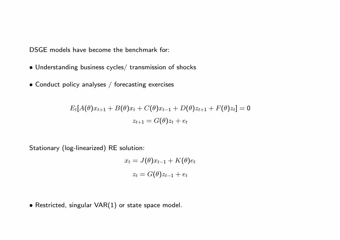
DSGE models have become the benchmark for:

• Understanding business cycles/ transmission of shocks

• Conduct policy analyses / forecasting exercises

Et[A(θ)xt+1 +B(θ)xt + C(θ)xt−1 +D(θ)zt+1 + F (θ)zt] = 0

zt+1 = G(θ)zt + et

Stationary (log-linearized) RE solution:

xt = J(θ)xt−1 +K(θ)et

zt = G(θ)zt−1 + et

• Restricted, singular VAR(1) or state space model.

How are DSGE estimated/evaluated?

1. Limited information methods

i. GMM

ii. Indirect Inference:

”minimum distance” estimation → matching impulse responses

iii. SVAR (magnitude and sign restrictions (Canova (2002)).

2. Full Information methods:

i. Maximum Likelihood

ii. Bayesian methods

3. Business cycle accounting/calibration

Chari et. al. (2007)

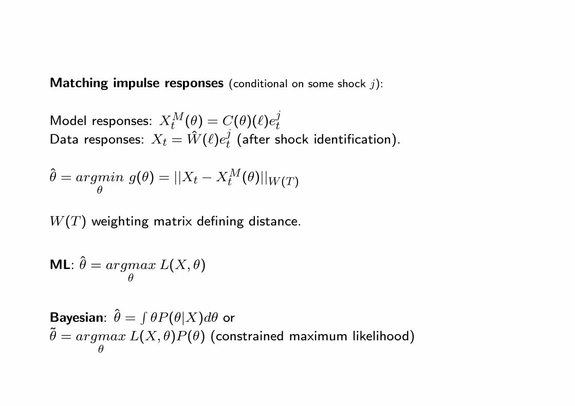
Matching impulse responses (conditional on some shock j):

Model responses: XMt (θ) = C(θ)( )e

jt

Data responses: Xt = W ( )ejt (after shock identification).

θ = argminθ

g(θ) = ||Xt −XMt (θ)||W (T )

W (T ) weighting matrix defining distance.

ML: θ = argmaxθ

L(X, θ)

Bayesian: θ =RθP (θ|X)dθ or

θ = argmaxθ

L(X, θ)P (θ) (constrained maximum likelihood)

Preliminary to estimation: can we recover structural parameters?

Identifiability:

Mapping from objective function to the parameters well behaved

• In general need:

- Objective function has a unique minimum 0 at θ = θ0- Hessian is positive definite and has full rank

- Curvature of objective function is ”sufficient”

Difficult to verify in practice because:

A) Mapping from structural parameters to solution parameters is unknown

(numerical solution)

B) Objective function is typically nonlinear function of solution parameters.

Different objective functions may have different ”identification power”

Standard rank and order conditions can’t be used!!!

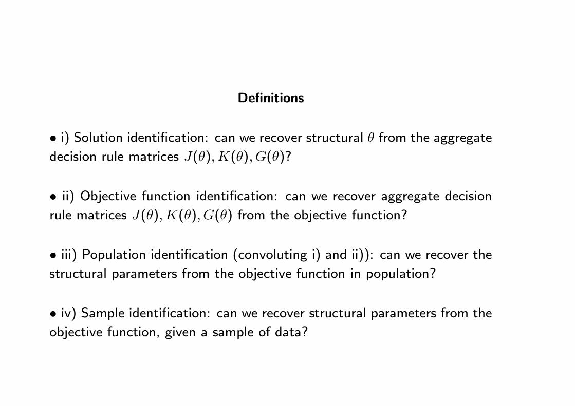
Definitions

• i) Solution identification: can we recover structural θ from the aggregate

decision rule matrices J(θ),K(θ), G(θ)?

• ii) Objective function identification: can we recover aggregate decisionrule matrices J(θ),K(θ), G(θ) from the objective function?

• iii) Population identification (convoluting i) and ii)): can we recover thestructural parameters from the objective function in population?

• iv) Sample identification: can we recover structural parameters from the

objective function, given a sample of data?

Note:

- i) and ii) can occur separately or in conjunction

- i) is due to the model specification, ii) may result from the choice of

objective function

- iv) may occur even if iii) does not

- iv) the focus of much of the econometric literature. Here focus on i) and

ii).

Preview:

Problems with DSGE models are in the solution/objective function map-

ping.

What kind of population problems may DSGE models encounter?

• Observational equivalence of models. Two models may have the same(minimized) value of the objective function at two different vector of pa-

rameters (e.g. a sticky price and a stocky wage model)

• Observational equivalence within a model. Two vectors of parametersmay give the same (minimized) value of the objective function, given a

model (e.g. given a sticky price model, get the same responses if Calvo

parameter is 0.25 or 0.75).

• Limited Information identification. A subset of the parameters of the

model can’t be identified because objective function uses only a portion of

the restrictions of the solution.

• Partial/under identification within a model. A subset of the structuralparameter enter in a particular functional form in the solution/ may disap-

pear from the solution.

• Weak/asymmetric identification within a model. The population map-ping is very flat or asymmetric in some dimension.

Local vs. global.

Could be due to particular objective function/occur for all objective func-

tions.

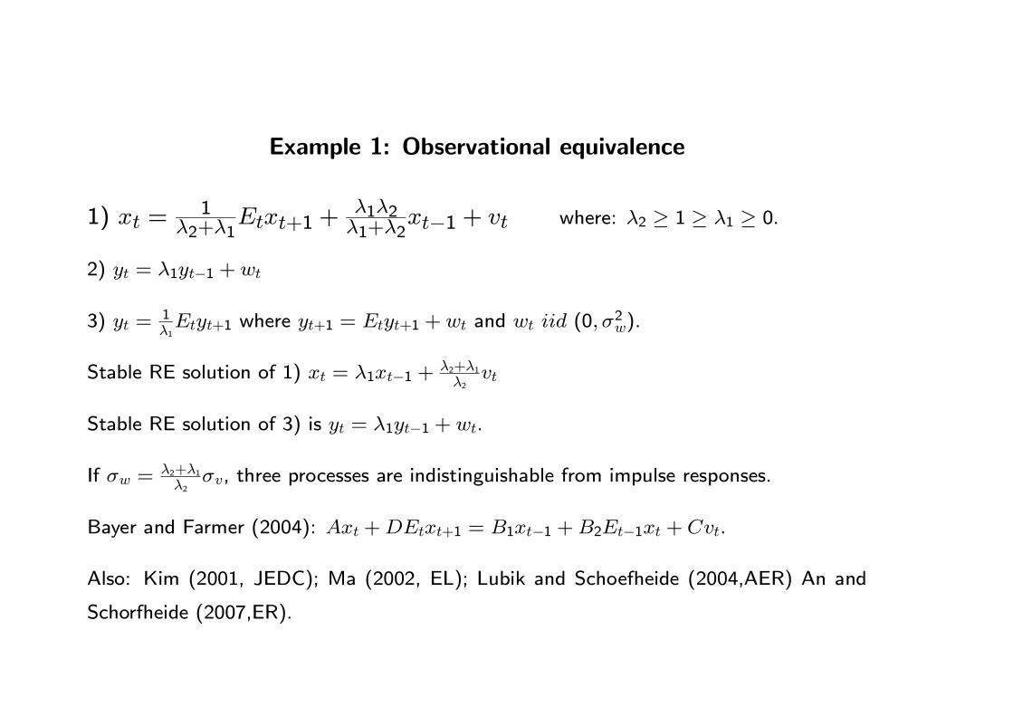
Example 1: Observational equivalence

1) xt =1

λ2+λ1Etxt+1 +

λ1λ2λ1+λ2

xt−1 + vt where: λ2 ≥ 1 ≥ λ1 ≥ 0.

2) yt = λ1yt−1 + wt

3) yt =1λ1Etyt+1 where yt+1 = Etyt+1 + wt and wt iid (0, σ2w).

Stable RE solution of 1) xt = λ1xt−1 +λ2+λ1λ2

vt

Stable RE solution of 3) is yt = λ1yt−1 + wt.

If σw =λ2+λ1λ2

σv, three processes are indistinguishable from impulse responses.

Bayer and Farmer (2004): Axt +DEtxt+1 = B1xt−1 +B2Et−1xt + Cvt.

Also: Kim (2001, JEDC); Ma (2002, EL); Lubik and Schoefheide (2004,AER) An and

Schorfheide (2007,ER).

Example 2: Under-identification

yt = a1Etyt+1 + a2(it −Etπt+1) + v1t (1)

πt = a3Etπt+1 + a4yt + v2t (2)

it = a5Etπt+1 + v3t (3)

Solution: ⎡⎣ ytπtit

⎤⎦ =⎡⎣ 1 0 a2

a4 1 a2a40 0 1

⎤⎦⎡⎣ v1tv2tv3t

⎤⎦• a1, a3, a5 disappear from the solution.

• Different shocks identify different parameters.• ML and distance could have different identification properties.

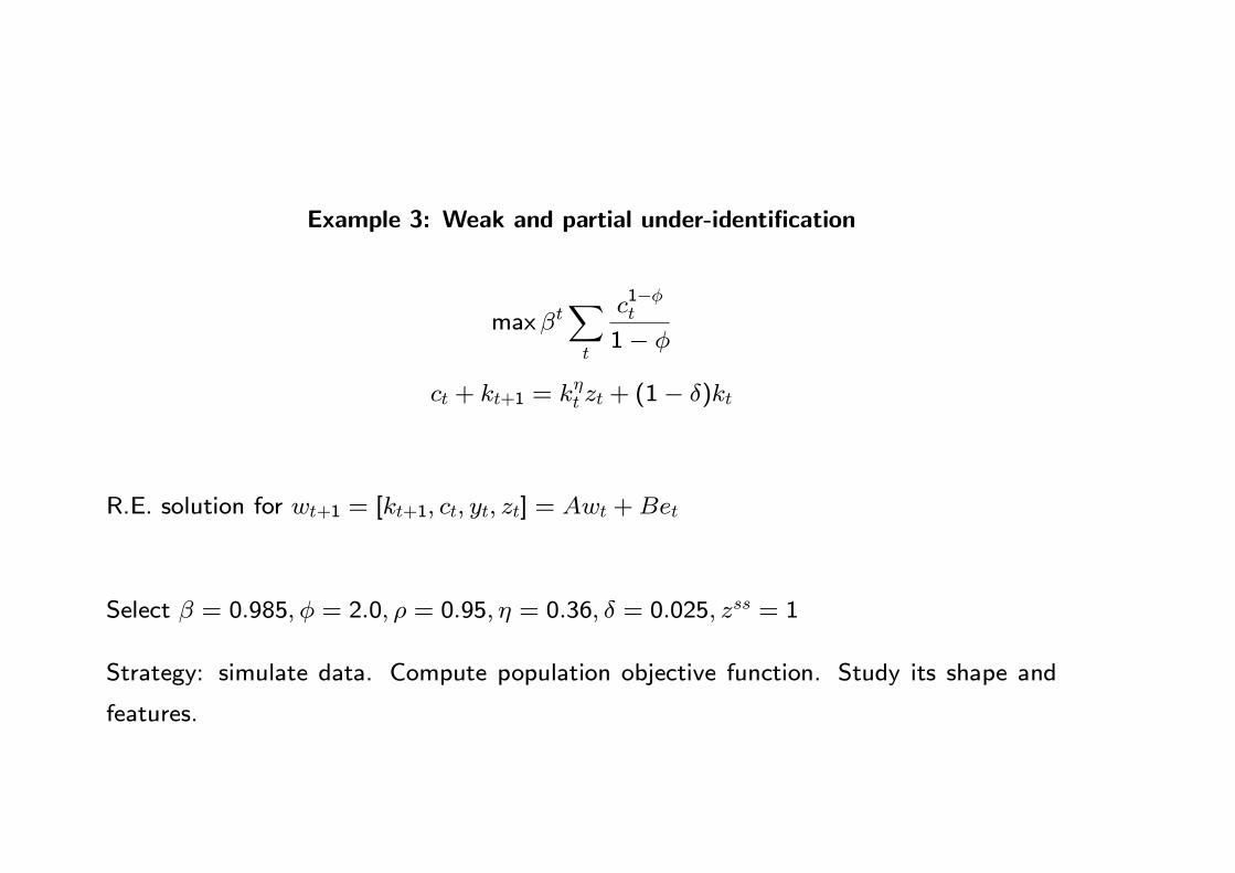
Example 3: Weak and partial under-identification

maxβtXt

c1−φt

1− φ

ct + kt+1 = kηt zt + (1− δ)kt

R.E. solution for wt+1 = [kt+1, ct, yt, zt] = Awt +Bet

Select β = 0.985, φ = 2.0, ρ = 0.95, η = 0.36, δ = 0.025, zss = 1

Strategy: simulate data. Compute population objective function. Study its shape and

features.

12

3

0.80.85

0.90.95

-20

-15

-10

-5

0

φρ 1 2 3

0.8

0.85

0.9

0.95

φ

ρ

-0.01 -0.05-0.05-0.5

-0.5

-1

-1

-5

-5

-10

0.010.02

0.03

0.9850.99

0.995-10

-8

-6

-4

-2

δβ 0.01 0.02 0.03

0.982

0.984

0.986

0.988

0.99

0.992

0.994

δ

β

-0.0

1-0

.01

-0.0

5-0.1

-0.5-1

12

3

0.80.85

0.90.95

-10

-5

0

φρ 1 2 3

0.8

0.85

0.9

0.95

φ

ρ

-0.01 -0.05-0.05-0.1-0.1

-0.5

-0.5

-1

-1

-5

0.010.02

0.03

0.9850.99

0.995-4

-3

-2

-1

δβ 0.01 0.02 0.03

0.982

0.984

0.986

0.988

0.99

0.992

0.994

ρ

φ

-0.00

5-0

.01

-0.05

-1

1

23

0.80.85

0.90.95

-0.2

-0.15

-0.1

-0.05

0

φρ 1 2 3

0.8

0.85

0.9

0.95

φ

ρ

-0.01

-0.01

-0.05

-0.05

-0.1

-0.1

0.010.02

0.03

0.9850.99

0.995-0.4

-0.3

-0.2

-0.1

δβ 0.01 0.02 0.03

0.982

0.984

0.986

0.988

0.99

0.992

0.994

δ

β

-0.0

01

-0.0

02-0.0

05-0.0

1

12

3

0.80.85

0.90.95

-2

-1.5

-1

-0.5

0

x 10-3

φρ 1 2 3

0.8

0.85

0.9

0.95

φ

ρ

-0.0001

-0.0001

-5e-005

-5e-005

0.010.02

0.03

0.9850.99

0.995-10

-8

-6

-4

-2

x 10-3

δβ 0.01 0.02 0.03

0.982

0.984

0.986

0.988

0.99

0.992

0.994

δ

β -0.0

005

-0.0

01

-0.0

02

-0.0

001

Figure 1: Distance surface: Basic, Subset, Matching VAR and Weighted

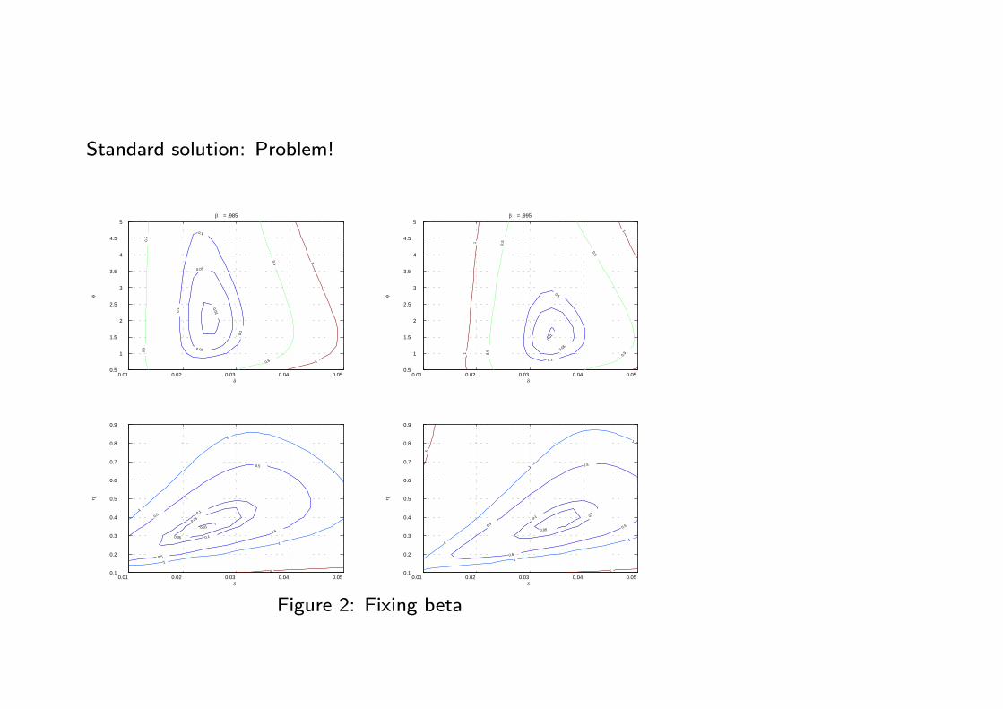
What causes the problems?

Law of motion of capital stock in almost invariant to :

(a) variations of η and ρ (weak identification)

(b) variations of β and δ additive (partial under-identification)

Can we reduce problems by:

(i) Changing W (T )? (long horizon may have little information)

(ii) Matching VAR coefficients?

(iii) Altering the objective function?

NO

Standard solution: Problem!

0.01 0.02 0.03 0.04 0.050.5

1

1.5

2

2.5

3

3.5

4

4.5

5

δ

φ

β = .985

0.01

0.05

0.05

0.1

0.1

0.1

0.5

0 .5

0.5

0.5

1

1

0.01 0.02 0.03 0.04 0.050.5

1

1.5

2

2.5

3

3.5

4

4.5

5

δφ

β = .995

0.01

0.05

0.1

0.1

0.5

0.5

0.5

0.51

1

1

0.01 0.02 0.03 0.04 0.050.1

0.2

0.3

0.4

0.5

0.6

0.7

0.8

0.9

δ

η

0.01

0.05

0.05

0.1

0.10.5

0.5

0.5

0.5

1

1

1

1

1

5

0.01 0.02 0.03 0.04 0.050.1

0.2

0.3

0.4

0.5

0.6

0.7

0.8

0.9

δ

η

0.05

0.1 0.1

0.5

0.5

0.5

0.5

1

1

1

1

1

5

5

Figure 2: Fixing beta

Identification and objective function

What objective function should one use? Likelihood!!

It has all the information and can be computed with Kalman filter.

What does a prior do? Can help is identification problems are due to small samples but

not if due to population problems!!

0.0220.0240.0260.0280.03

0.9750.98

0.9850.99

0.995-10000

-5000

0

δβ

0.0220.0240.0260.0280.03

0.9750.98

0.9850.99

0.995-4

-2

0

x 10 4

δβ

0.022 0.024 0.026 0.028 0.030.975

0.98

0.985

0.99

0.995

δ

β -10-100

-100

-100

-1000

-1000

0.022 0.024 0.026 0.028 0.030.975

0.98

0.985

0.99

0.995

δ

β -100

-1000

-1000

Figure 3: Likelihood and Posterior

Posterior not usually updated if likelihood has no information.

With constraints, updating is possible (many constraints from the model).

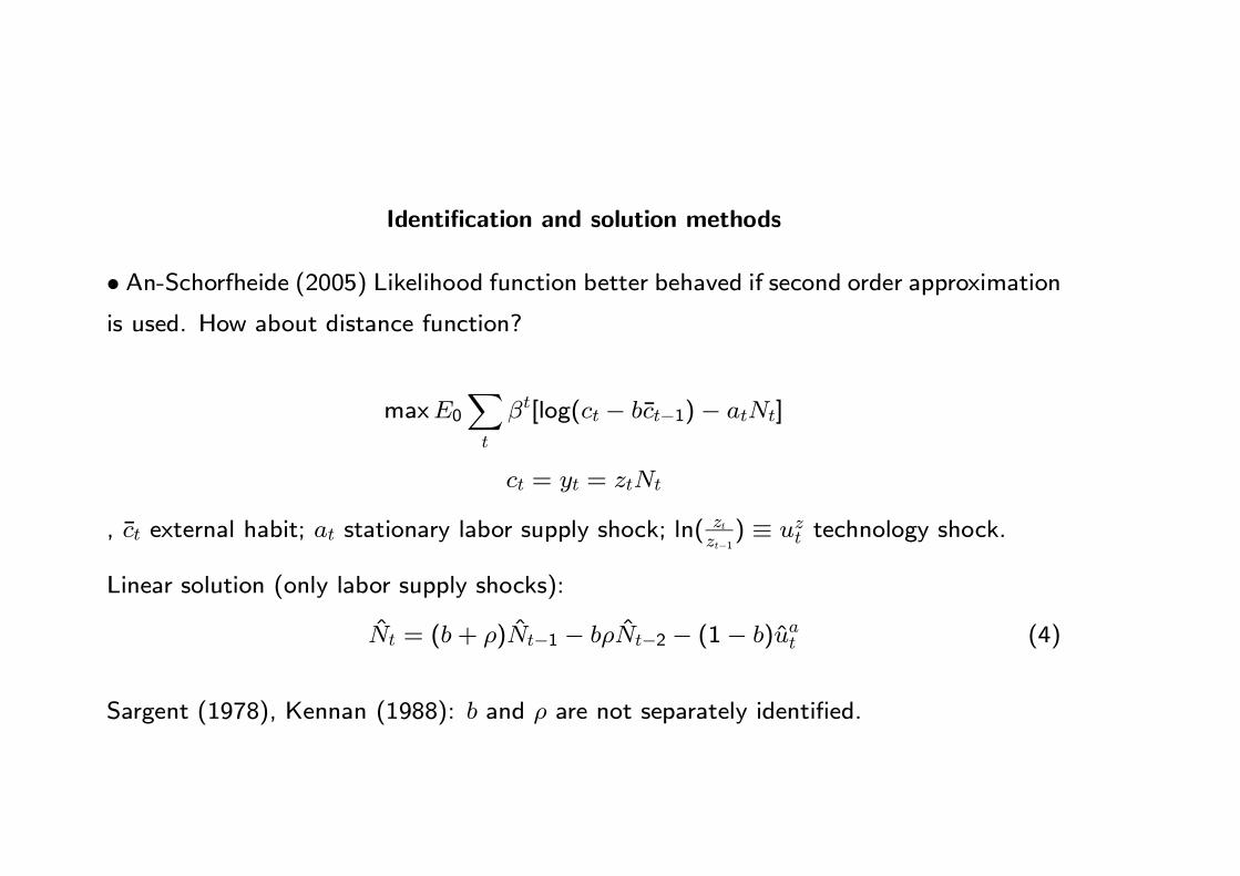
Identification and solution methods

• An-Schorfheide (2005) Likelihood function better behaved if second order approximationis used. How about distance function?

maxE0Xt

βt[log(ct − bct−1)− atNt]

ct = yt = ztNt

, ct external habit; at stationary labor supply shock; ln(ztzt−1) ≡ uzt technology shock.

Linear solution (only labor supply shocks):

Nt = (b+ ρ)Nt−1 − bρNt−2 − (1− b)uat (4)

Sargent (1978), Kennan (1988): b and ρ are not separately identified.

Second order solution (only labor supply shocks):

Nt = bNt−1 +b(b−1)2

N2t−1 − (1− b)at − 1

2(−(1− b)2 + 1− b)a2t

at = ρat−1 + uat

0.2 0.4 0.6 0.80.20.40.60.8

0

0.5

1

1.5

2

2.5

3

3.5

ρ

Responses to a labor supply shock

b

Rat

io o

f Cur

vatu

res

Figure 4: Distance function: linear vs. quadratic

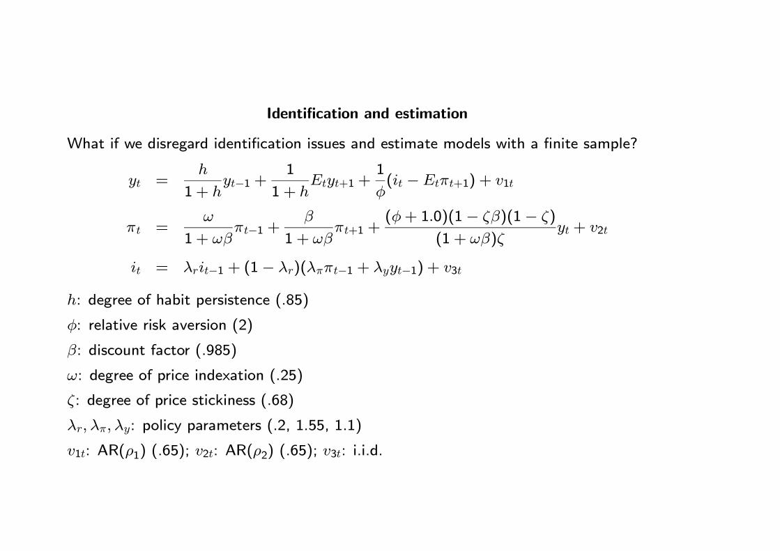
Identification and estimation

What if we disregard identification issues and estimate models with a finite sample?

yt =h

1 + hyt−1 +

1

1 + hEtyt+1 +

1

φ(it −Etπt+1) + v1t

πt =ω

1 + ωβπt−1 +

β

1 + ωβπt+1 +

(φ+ 1.0)(1− ζβ)(1− ζ)

(1 + ωβ)ζyt + v2t

it = λrit−1 + (1− λr)(λππt−1 + λyyt−1) + v3t

h: degree of habit persistence (.85)

φ: relative risk aversion (2)

β: discount factor (.985)

ω: degree of price indexation (.25)

ζ: degree of price stickiness (.68)

λr, λπ, λy: policy parameters (.2, 1.55, 1.1)

v1t: AR(ρ1) (.65); v2t: AR(ρ2) (.65); v3t: i.i.d.

0.98 0.985 0.990

2

4

x 10-3

β =

0.98

5

0.98 0.985 0.990

2

4

x 10-3

0.98 0.985 0.990

2

4

x 10-3

0.98 0.985 0.990

2

4

x 10-3

1 2 30

10

20

φ =

2

1 2 30

10

20

1 2 30

10

20

1 2 30

10

20

0 2 40

5

10

ν =

3

0 2 40

5

10

0 2 40

5

10

0 2 40

5

10

0.5 0.6 0.7 0.8 0.90

50100150

ξ =

0.68

0.5 0.6 0.7 0.8 0.90

50100150

0.5 0.6 0.7 0.8 0.90

50100150

0.5 0.6 0.7 0.8 0.90

50100150

0.1 0.2 0.30

0.5

1

λ r = 0

.2

0.1 0.2 0.30

0.5

1

0.1 0.2 0.30

0.5

1

0.1 0.2 0.30

0.5

1

1.2 1.4 1.6 1.8 20123

λ π = 1

.55

1.2 1.4 1.6 1.8 20123

1.2 1.4 1.6 1.8 20123

1.2 1.4 1.6 1.8 20123

0.9 1 1.1 1.2 1.30

0.10.2

0.3

λ y = 1

.1

0.9 1 1.1 1.2 1.30

0.10.2

0.3

0.9 1 1.1 1.2 1.30

0.10.2

0.3

0.9 1 1.1 1.2 1.30

0.10.2

0.3

0.6 0.65 0.70

0.5

1

ρ 1 = 0

.65

0.6 0.65 0.70

0.5

1

0.6 0.65 0.70

0.5

1

0.6 0.65 0.70

0.5

1

0.6 0.65 0.70

0.5

1

ρ 2 = 0

.65

0.6 0.65 0.70

0.5

1

0.6 0.65 0.70

0.5

1

0.6 0.65 0.70

0.5

1

0.5 0.6 0.7 0.8 0.90

0.2

0.4

0.6

ω =

0.7

0.5 0.6 0.7 0.8 0.90

0.2

0.4

0.6

0.5 0.6 0.7 0.8 0.90

0.2

0.4

0.6

0.5 0.6 0.7 0.8 0.90

0.2

0.4

0.6

0.7 0.8 0.9 10

0.020.040.06

IS shock

h =

0.85

0.7 0.8 0.9 10

0.020.040.06

Cost push shock0.7 0.8 0.9 1

00.020.040.06

Monetary policy shock0.7 0.8 0.9 1

00.020.040.06

All shocks

Figure 5: Distance function shape

2 4 6 8 10 12

0.6

0.7

0.8-0.5-0.4-0.3-0.2-0.1

ν

Monetary shocks

ξ

2 4 6 8 10 120.6

0.65

0.7

0.75

0.8

ν

ξ

0.001

0.001

0.001

0.001

0.01

0.01

0.01

0.01

0.1

0.1

0.3

2 4 6 8 10 12

0.6

0.7

0.8-20

-15

-10

-5

0

ν

Cost push shocks

ξ

2 4 6 8 10 120.6

0.65

0.7

0.75

0.8

ν

ξ 0.01

0.010.01

0.01

0.1

0.10.1

0.1

0.3

0.3

0.3

0.3

0.5

0.5

0.5

0.5

0.7

0.7

0.7

0.9

0.9

0.9

2

2

5

0.81

1.21.41.5

2-0.04

-0.02

0

λ yλ

π

0.8 1 1.2 1.4

1.2

1.4

1.6

1.8

2

λ y

λ π

0.001

0.0010.001

0.01

0.01

0.81

1.21.41.5

2-2

-1

0

λ yλ

π

0.8 1 1.2 1.4

1.2

1.4

1.6

1.8

2

λ y

λ π

0.01

0.01

0.1

0.1

0.1

0.1

0.3

0.3

0.3

0.5

0.5

0.7 0.9

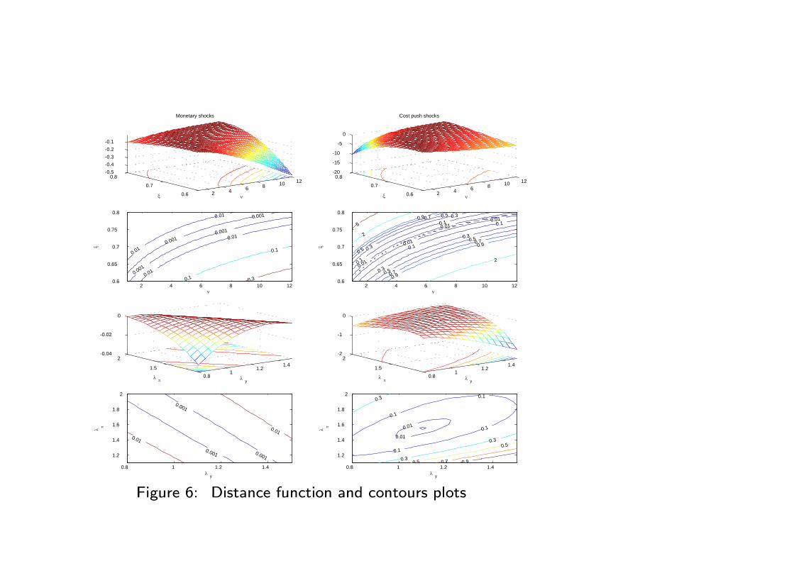
Figure 6: Distance function and contours plots

0.975 0.98 0.985 0.99 0.9950

20

40

60

80β = 0.985

2 4 6 80

50

100

φ = 2

0.2 0.4 0.6 0.80

20

40

60

ζ = 0.68

0.2 0.4 0.6 0.80

50

100λ r = 0.2

2 4 6 80

50

100

λπ

= 1.55

1 2 3 40

50

100

0.2 0.4 0.6 0.80

10

20

ρ 1 = 0.65

0.2 0.4 0.6 0.80

10

20

30ρ 2 = 0.65

0.2 0.4 0.6 0.80

50

100

150ω = 0.25

0.2 0.4 0.6 0.80

50

100h = 0.85

λ y = 1.1

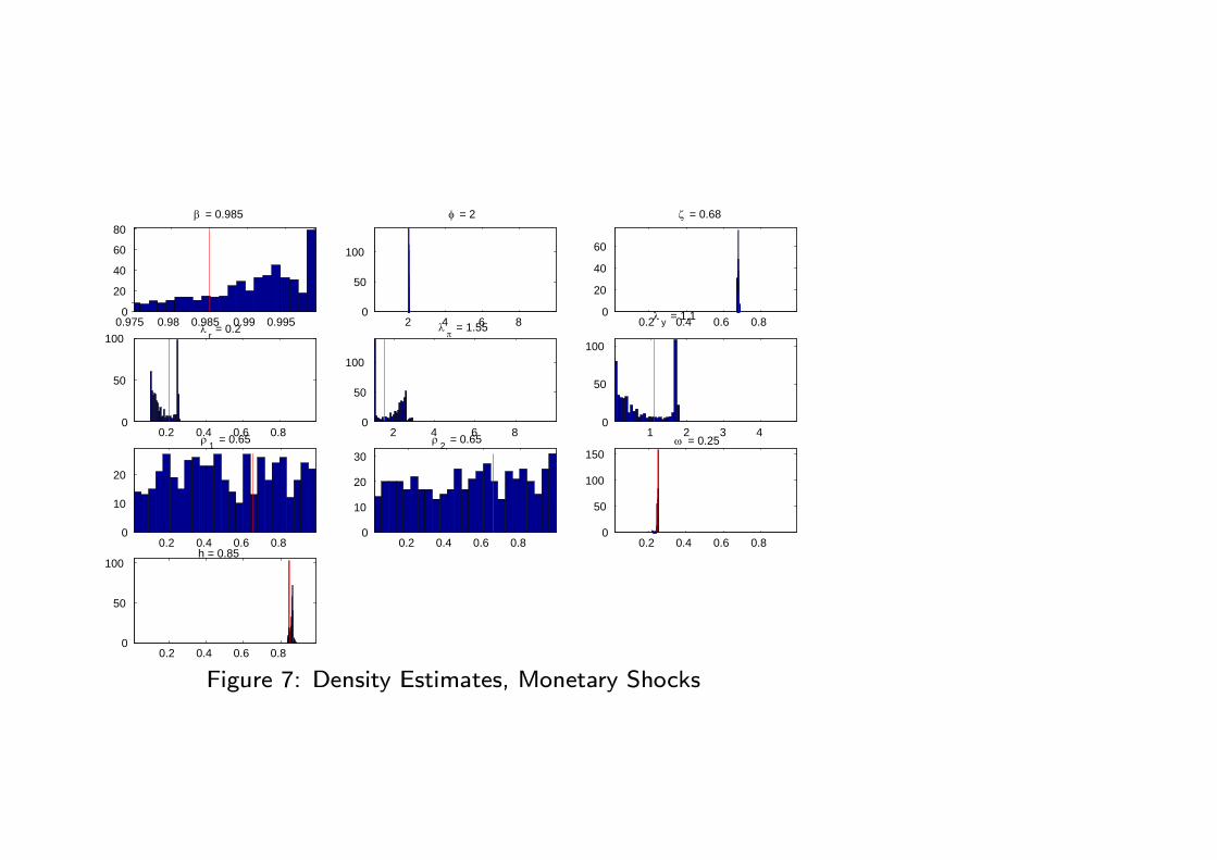
Figure 7: Density Estimates, Monetary Shocks

0 10 20-0.2

0

0.2

0.4

0.6

0.8

1

1.2

1.4Gap

IS

0 10 200

0.2

0.4

0.6

0.8

1

1.2

1.4π

0 10 200

0.5

1

1.5

2

2.5

3interest rate

0 10 20-1.5

-1

-0.5

0

0.5

Cos

t pus

h

0 10 20-0.5

0

0.5

1

1.5

2

2.5

0 10 20-0.5

0

0.5

1

1.5

2

2.5

0 10 20-0.5

-0.4

-0.3

-0.2

-0.1

0

0.1

0.2

Mon

etar

y

0 10 20-0.3

-0.25

-0.2

-0.15

-0.1

-0.05

0

0.05

0 10 20-0.6

-0.4

-0.2

0

0.2

0.4

0.6

0.8

1

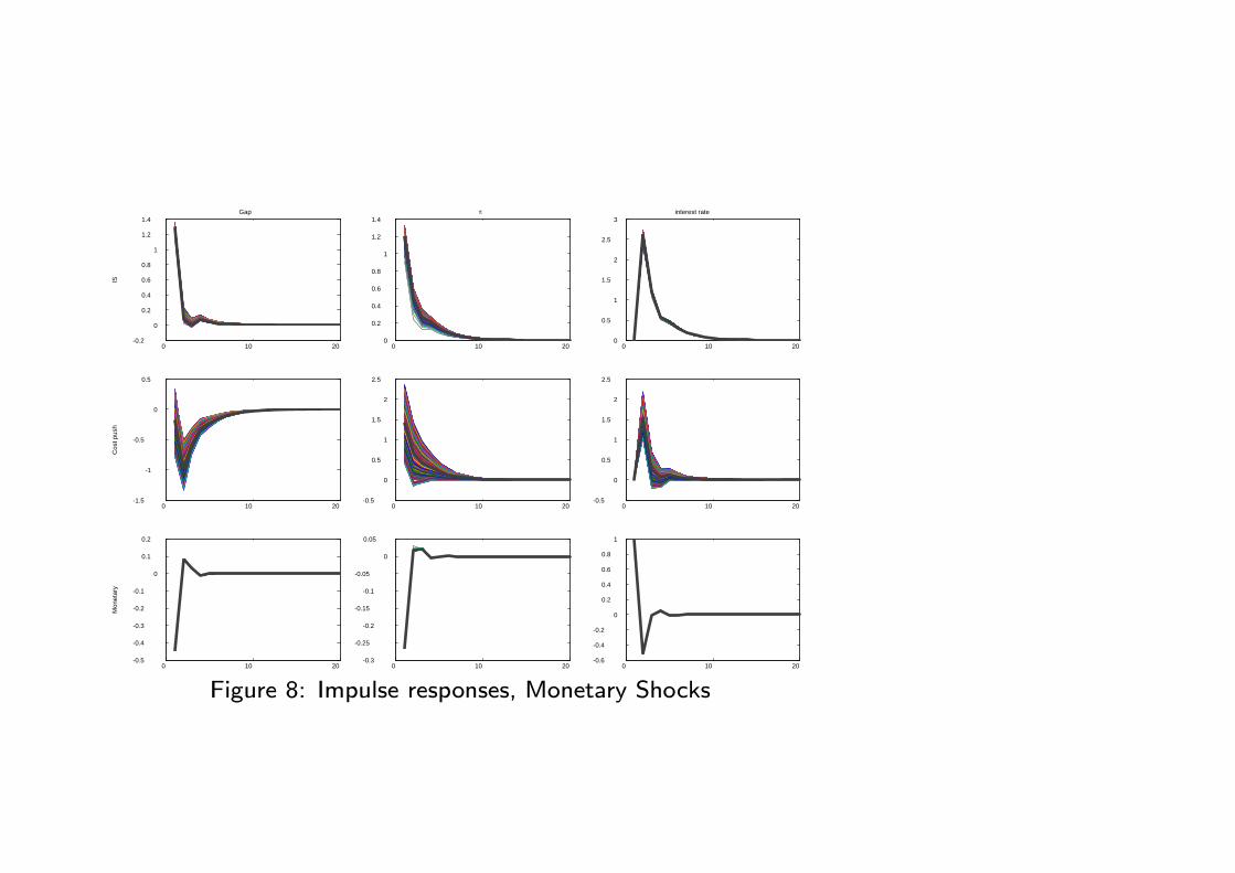
Figure 8: Impulse responses, Monetary Shocks

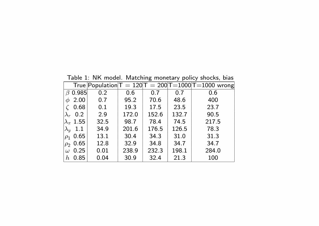
Table 1: NK model. Matching monetary policy shocks, biasTrue PopulationT = 120T = 200T=1000T=1000 wrong

β 0.985 0.2 0.6 0.7 0.7 0.6φ 2.00 0.7 95.2 70.6 48.6 400ζ 0.68 0.1 19.3 17.5 23.5 23.7λr 0.2 2.9 172.0 152.6 132.7 90.5λπ 1.55 32.5 98.7 78.4 74.5 217.5λy 1.1 34.9 201.6 176.5 126.5 78.3ρ1 0.65 13.1 30.4 34.3 31.0 31.3ρ2 0.65 12.8 32.9 34.8 34.7 34.7ω 0.25 0.01 238.9 232.3 198.1 284.0h 0.85 0.04 30.9 32.4 21.3 100

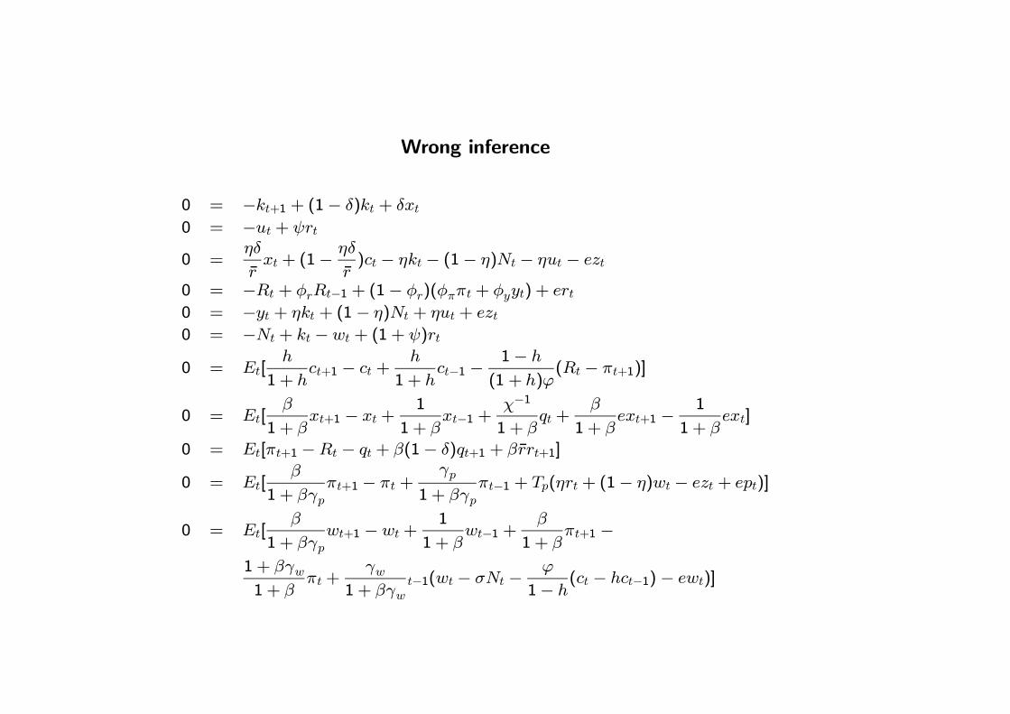
Wrong inference

0 = −kt+1 + (1− δ)kt + δxt0 = −ut + ψrt

0 =ηδ

rxt + (1−

ηδ

r)ct − ηkt − (1− η)Nt − ηut − ezt

0 = −Rt + φrRt−1 + (1− φr)(φππt + φyyt) + ert0 = −yt + ηkt + (1− η)Nt + ηut + ezt0 = −Nt + kt −wt + (1 + ψ)rt

0 = Et[h

1 + hct+1 − ct +

h

1 + hct−1 −

1− h

(1 + h)ϕ(Rt − πt+1)]

0 = Et[β

1 + βxt+1 − xt +

1

1 + βxt−1 +

χ−1

1 + βqt +

β

1 + βext+1 −

1

1 + βext]

0 = Et[πt+1 −Rt − qt + β(1− δ)qt+1 + βrrt+1]

0 = Et[β

1 + βγpπt+1 − πt +

γp

1 + βγpπt−1 + Tp(ηrt + (1− η)wt − ezt + ept)]

0 = Et[β

1 + βγpwt+1 −wt +

1

1 + βwt−1 +

β

1 + βπt+1 −

1 + βγw1 + β

πt +γw

1 + βγwt−1(wt − σNt −

ϕ

1− h(ct − hct−1)− ewt)]

δ depreciation rate (.0182) λw wage markup (1.2)ψ parameter (.564) π steady state π (1.016)η share of capital (.209) h habit persistence (.448)ϕ risk aversion (3.014) σl inverse elasticity of labor supply (2.145)β discount factor (.991) χ−1 investment’s elasticity to Tobin’s q (.15)ζp price stickiness (.887) ζw wage stickiness (.62)γp price indexation (.862) γw wage indexation (.221)φy response to y (.234) φπ response to π (1.454)φr int. rate smoothing (.779)

Tp ≡ (1−βζp)(1−ζp)(1+βγp)ζp

Tw ≡ (1−βζw)(1−ζw)(1+β)(1+(1+λw)σlλ

−1w )ζw

0.015 0.02

x 10-7

δ = 0.0180.2 0.25

0

1

2

3

4

5

6

7

8

9

10x 10

-7

η = 0.2090.988 0.99 0.992 0.994

0

1

2

3

4

5

6

7

8

9

10x 10

-7

β = 0.9910.4 0.45 0.5

0

1

2

3

4

5

6

7

8

9

10x 10

-7

h = 0.4485 6 7

0

1

2

3

4

5

6

7

8

9

10x 10

-7

χ = 6.32.5 3 3.5

0

1

2

3

4

5

6

7

8

9

10x 10

-7

φ = 3.014

2 3

x 10-7

ν = 2.1450.5 0.6

0

1

2

3

4

5

6

7

8

9

10x 10

-7

ψ = 0.5640.85 0.9

0

1

2

3

4

5

6

7

8

9

10x 10

-7

ξp

= 0.8870.8 0.9

0

1

2

3

4

5

6

7

8

9

10x 10

-7

γp

= 0.8620.6 0.7

0

1

2

3

4

5

6

7

8

9

10x 10

-7

ξw

= 0.620.15 0.2 0.25

0

1

2

3

4

5

6

7

8

9

10x 10

-7

γw

= 0.221

1.15 1.2 1.25

x 10-7

εw

= 1.20.2 0.3

0

1

2

3

4

5

6

7

8

9

10x 10

-7

λy

= 0.2341.45 1.5

0

1

2

3

4

5

6

7

8

9

10x 10

-7

λπ

= 1.4540.75 0.8

0

1

2

3

4

5

6

7

8

9

10x 10

-7

λr = 0.779

0.98 0.99 1

0

1

2

3

4

5

6

7

8

9

10x 10

-7

ρz

= 0.997

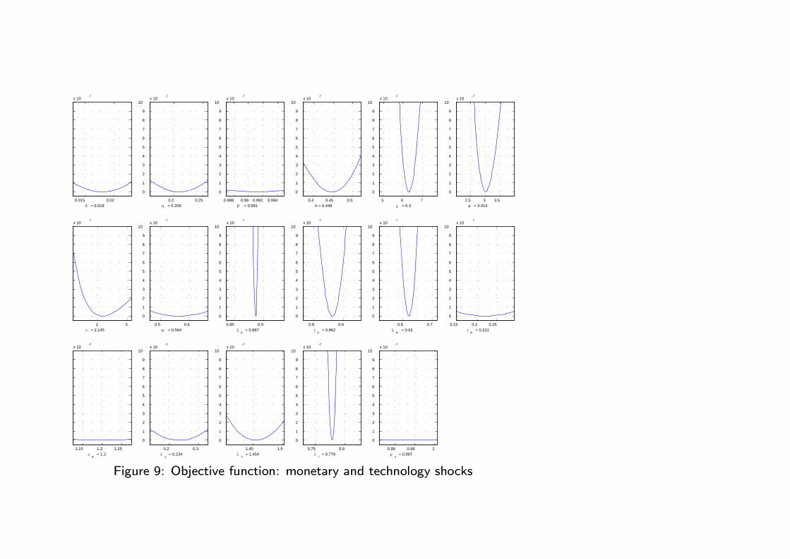
Figure 9: Objective function: monetary and technology shocks

00.5

1

0

0.5

1-2

0

x 10 -4

γ pξ p

dist

ance

0.2 0.4 0.6 0.8

0.2

0.4

0.6

0.8

γ p

ξ p

-0.00015

-0.0001

-0.0001

-1e-005-1e-005

0.2 0.4 0.6 0.80.2

0.40.6

0.8

-0.03

-0.02

-0.01

γ wξ w

dist

ance

0.2 0.4 0.6 0.8

0.2

0.4

0.6

0.8

γ w

ξ w

-0.0001-0.0005

-5e-005-1e-005

-1e-005

-5e-006

-5e-006

0.2 0.4 0.6 0.8

0.20.4

0.60.8

-5-4-3-2-1

x 10 -5

γ pγ w

dist

ance

0.2 0.4 0.6 0.8

0.2

0.4

0.6

0.8

γ p

γ w

-1e-005

-5e-006

-1e-006

-1e-006-5e-007

0.2 0.4 0.6 0.8

0.20.4

0.60.8

-15

-10

-5

x 10 -3

ξ pξ w

dist

ance

0.2 0.4 0.6 0.8

0.2

0.4

0.6

0.8

ξ p

ξ w

-0.0005 -0.00045-0.00035-0.00025-0.00015

-0.0001

Figure 10: Distance surface and Contours Plots

ζp γp ζw γw Obj.Fun.Baseline 0.887 0.862 0.62 0.221

x0 = lb + 1std 0.8944 0.8251 0.615 0 1.8235E-07x0 = lb + 2std 0.8924 0.7768 0.6095 0.1005 3.75E-07x0 = ub - 1std 0.882 0.7957 0.6062 0.1316 2.43E-07x0 = ub - 2std 0.9044 0.7701 0.6301 0 8.72E-07

Case 1 0 0.862 0.62 0.221x0 = lb + 1std 0.1304 0.0038 0.6401 0.245 2.7278E-08x0 = lb + 2std 0.1015 0.0853 0.6065 0.1791 4.84E-08x0 = ub - 1std 0.0701 0.1304 0.6128 0.1979 4.72E-08x0 = ub - 2std 0.0922 0.0749 0.618 0.215 3.05E-08

Case 2 0 0 0.62 0.221x0 = lb + 1std 0.1396 0.0072 0.6392 0.2436 3.1902E-08x0 = lb + 2std 0.0838 0.1193 0.6044 0.1683 4.38E-08x0 = ub - 1std 0.0539 0.1773 0.6006 0.1575 5.51E-08x0 = ub - 2std 0.0789 0.0971 0.6114 0.1835 2.61E-08

Case 3 0 0.862 0.62 0x0 = lb + 1std 0.0248 0 0.6273 0.029 7.437E-09x0 = lb + 2std 0.4649 0 0.7443 0.4668 2.10E-06x0 = ub - 1std 0.0652 0.0004 0.6147 0.0447 7.13E-08x0 = ub - 2std 0.6463 0.2673 0.8222 0.3811 5.56E-06

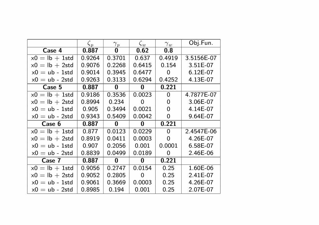
ζp γp ζw γw Obj.Fun.Case 4 0.887 0 0.62 0.8

x0 = lb + 1std 0.9264 0.3701 0.637 0.4919 3.5156E-07x0 = lb + 2std 0.9076 0.2268 0.6415 0.154 3.51E-07x0 = ub - 1std 0.9014 0.3945 0.6477 0 6.12E-07x0 = ub - 2std 0.9263 0.3133 0.6294 0.4252 4.13E-07

Case 5 0.887 0 0 0.221x0 = lb + 1std 0.9186 0.3536 0.0023 0 4.7877E-07x0 = lb + 2std 0.8994 0.234 0 0 3.06E-07x0 = ub - 1std 0.905 0.3494 0.0021 0 4.14E-07x0 = ub - 2std 0.9343 0.5409 0.0042 0 9.64E-07

Case 6 0.887 0 0 0.221x0 = lb + 1std 0.877 0.0123 0.0229 0 2.4547E-06x0 = lb + 2std 0.8919 0.0411 0.0003 0 4.26E-07x0 = ub - 1std 0.907 0.2056 0.001 0.0001 6.58E-07x0 = ub - 2std 0.8839 0.0499 0.0189 0 2.46E-06

Case 7 0.887 0 0 0.221x0 = lb + 1std 0.9056 0.2747 0.0154 0.25 1.60E-06x0 = lb + 2std 0.9052 0.2805 0 0.25 2.41E-07x0 = ub - 1std 0.9061 0.3669 0.0003 0.25 4.26E-07x0 = ub - 2std 0.8985 0.194 0.001 0.25 2.07E-07

0 5 10 15 20-0.1

-0.08

-0.06

-0.04

-0.02

0

0.02Inflation

0 5 10 15 20-0.1

0

0.1

0.2

0.3Interest rate

0 5 10 15 20-1.5

-1

-0.5

0Real wage

0 5 10 15 20-0.8

-0.6

-0.4

-0.2

0Investment

0 5 10 15 20-0.25

-0.2

-0.15

-0.1

-0.05

0Consumption

0 5 10 15 20-0.2

-0.15

-0.1

-0.05

0

0.05Hours worked

0 5 10 15 20-0.25

-0.2

-0.15

-0.1

-0.05

0output

quarters after shock0 5 10 15 20

-0.6

-0.4

-0.2

0

0.2Capacity utilisation

quarters after shock

TrueEstimated

Figure 11: Impulse responses, Case 5.

Welfare costs different!

L(π2, y2) = −0.0005 with true parameters

L(π2, y2) = −0.0022 with estimated parameters

Detecting identification problems:

Ex-ante diagnostics:

- Plots/ Preliminary exploration of objective function

- Numerical derivatives of the objective function at likely parameter values

- Condition number of the Hessian (ratio largest/smallest eigenvalues)

Ex-post diagnostics:

- Erratic parameter estimates as T increases

- Large or non-computable standard errors

- Crazy t-test (Choi and Phillips (1992), Stock and Wright (2003)).

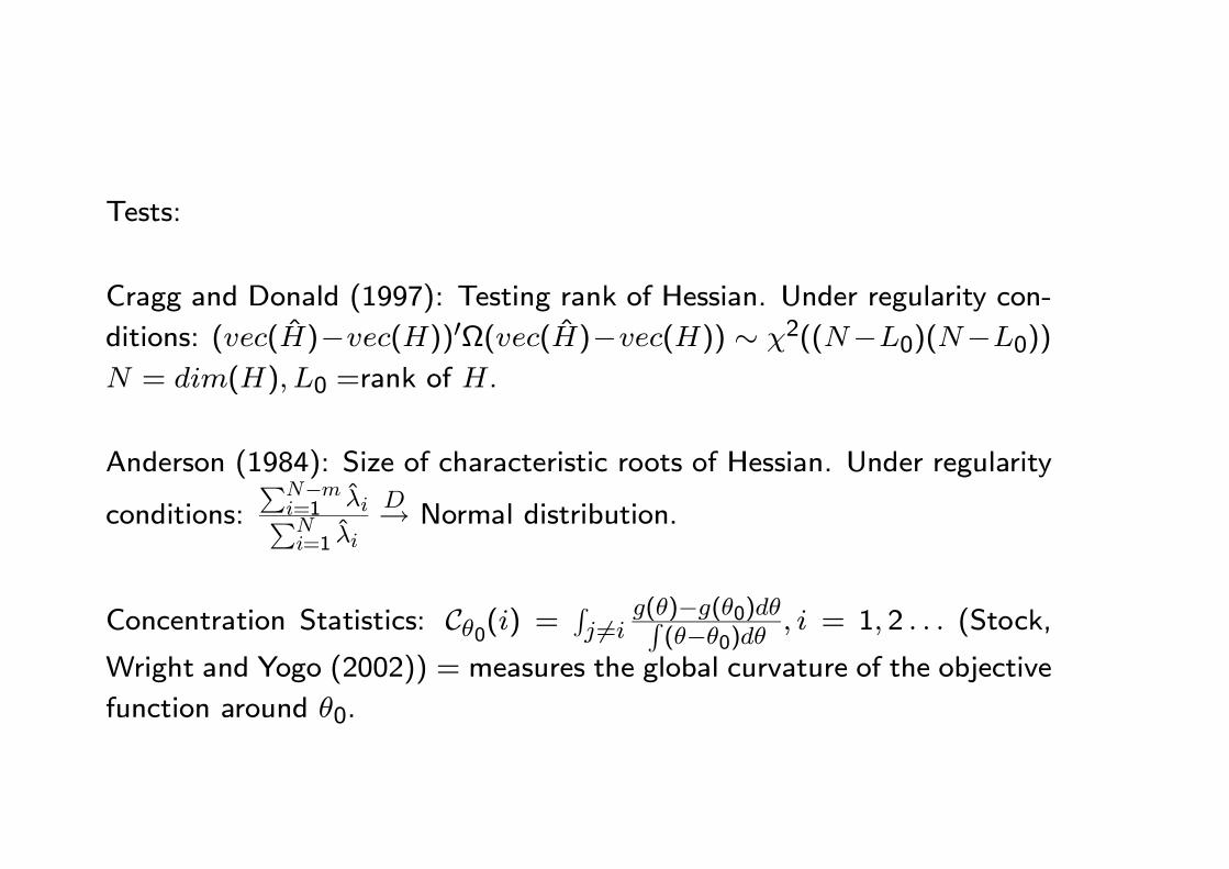
Tests:

Cragg and Donald (1997): Testing rank of Hessian. Under regularity con-

ditions: (vec(H)−vec(H))0Ω(vec(H)−vec(H)) ∼ χ2((N−L0)(N−L0))N = dim(H), L0 =rank of H.

Anderson (1984): Size of characteristic roots of Hessian. Under regularity

conditions:PN−m

i=1 λiPNi=1 λi

D→ Normal distribution.

Concentration Statistics: Cθ0(i) =Rj 6=i

g(θ)−g(θ0)dθR(θ−θ0)dθ

, i = 1, 2 . . . (Stock,

Wright and Yogo (2002)) = measures the global curvature of the objective

function around θ0.

Difficult to employ: just use as a diagnostic.

Applied to last model: rank of H = 6; sum of 12-13 characteristics roots

is smaller than 0.01 of the average root → 12-13 dimensions of weak or

partial identification problems.

Which are the parameters is causing problems?

β, h, σl, δ, η, ψ, γp, γw, λw, φπ, φy, ρz.

Why? Variations of these parameters hardly affect law of motion of states!

Almost a rule: for identification need states to react changes in structural

parameters.

What to do when identification problems exist?

Which type?

- If population need respecify the model.

- If objective/ limited information use likelihood.

- If small sample add information (prior or other data)

- Don´t proceed as if they do not exist.

- Careful with mixed calibration-estimation. Full calibration preferable or

Bayesian calibration (Canova (1995))

Conclusions:

• Liu (1960), Sims (1980):

- Traditional models hopelessly under-identified.

- Identification often achieved not because we have sufficient information

but because we want it to be so.

- Proceed with reduced form models

• A destructive approach:

- Most (large scale) DSGE models are face severe identification problems.

- Models are identified not because likelihood (or part of it) is informative,

but because we make it informative (via partial calibration or tight priors).

- Estimation = confirmatory analysis.

- Hard to reject models.

• A more constructive one:

(i) Try to respecify the model to get rid of problems

(ii) Evaluate numerically the mapping between structural parameters and

coefficients of the decision rule. Do extensive exploratory analysis.

(iii) Find out what estimation method could work also in presence of iden-

tification problems (Stock and Wright (2000), Rosen (2005))

(iv) Work out economic reasons for identification problems with submodels

or simplified versions of larger ones

(v) Be less demanding of your models. Use methodologies why employ

semi-structural estimation (e.g. SVARs)