Page 1
Escola Tècnica Superior d’Enginyeria Industrial de Barcelona
Treball de Fi de Master
Master’s degree in Automatic Control and Robotics
IDENTIFICATION AND CONTROL OF DC MOTORS
MEMÒRIA
Autor: Darshan Ramasubramanian Director/s: Dr. Vicenç Puig Cayuela Convocatòria: September 2016
Escola Tècnica Superior d’Enginyeria Industrial de Barcelona
Escola Tècnica Superior d’Enginyeria Industrial de Barcelona
Escola Tècnica Superior d’Enginyeria Industrial de Barcelona
Page 3
Abstract
This work has two main objectives: the first one is identify the model of DC motors - using various
techniques from experimental data; Secondly, we want to design appropriate control structures for
this system, so as to meet the specifications requested.
The second chapter describes the equipment with which we work throughout the project, consist-
ing of two rotary brushed DC motors provided by the company Ingenia Motion Control. The third
chapter describes various techniques of system identification that are used to characterize the motor
dynamics, and applied to the motors provided by the company Ingenia Motion Control. And the final
chapter covers the design of controllers plants based on the specification in bandwidth, and provides
detailed structures of PID control and I-PD control.
This master thesis has been developed in the Institut de Robòtica i Informàtica Industrial (IRI)
and in the company Ingenia Motion Control in the Firmware Division with the supervision of Vicenç
Puig as director and Roger Juanpere and Rob Verhaart as advisers from the company.
Page 5
Contents
1 Introduction 2
2 Background 3
2.1 General Description of DC motor . . . . . . . . . . . . . . . . . . . . . . . . . . . . . . . . 3
2.2 Control Structure . . . . . . . . . . . . . . . . . . . . . . . . . . . . . . . . . . . . . . . . . 4
2.2.1 Electrical Characteristics . . . . . . . . . . . . . . . . . . . . . . . . . . . . . . . . . 5
2.2.2 Mechanical Characterstics . . . . . . . . . . . . . . . . . . . . . . . . . . . . . . . . 6
2.3 Control Law . . . . . . . . . . . . . . . . . . . . . . . . . . . . . . . . . . . . . . . . . . . . 7
2.3.1 PI controller . . . . . . . . . . . . . . . . . . . . . . . . . . . . . . . . . . . . . . . . 9
2.3.2 PID controller . . . . . . . . . . . . . . . . . . . . . . . . . . . . . . . . . . . . . . . 9
3 Real Setup 12
4 System Identification 17
4.1 Design of Inputs . . . . . . . . . . . . . . . . . . . . . . . . . . . . . . . . . . . . . . . . . . 17
4.1.1 Current Loop . . . . . . . . . . . . . . . . . . . . . . . . . . . . . . . . . . . . . . . 18
4.1.2 Position Loop . . . . . . . . . . . . . . . . . . . . . . . . . . . . . . . . . . . . . . . 20
4.2 Analysis of Model Structure . . . . . . . . . . . . . . . . . . . . . . . . . . . . . . . . . . . 21
4.2.1 Process Models . . . . . . . . . . . . . . . . . . . . . . . . . . . . . . . . . . . . . . 21
4.2.2 Polynomial model . . . . . . . . . . . . . . . . . . . . . . . . . . . . . . . . . . . . 22
4.3 Identification methods . . . . . . . . . . . . . . . . . . . . . . . . . . . . . . . . . . . . . . 24
4.3.1 Electrical Identification . . . . . . . . . . . . . . . . . . . . . . . . . . . . . . . . . . 25
4.3.2 Mechanical Identification . . . . . . . . . . . . . . . . . . . . . . . . . . . . . . . . 31
II
Page 6
Identification and Control of DC Motors 1
5 Design of Controllers 43
5.1 Current Loop . . . . . . . . . . . . . . . . . . . . . . . . . . . . . . . . . . . . . . . . . . . 43
5.2 Position loop . . . . . . . . . . . . . . . . . . . . . . . . . . . . . . . . . . . . . . . . . . . . 47
6 Environment impact study 52
7 Conclusions 53
8 Cost of the project 55
9 Bibliography 59
A Matlab codes and Datasheet of Motors 60
Page 7
Chapter 1
Introduction
A servo drive system is a typical electrodynamic actuator for small high dynamic machine tool axes as
well as wire bonding machines and hydraulic/pneumatic valve drives. One of the special servo drive
system is the Brushed DC motors. The work is based on the desire to delve into the world of research
in the elds of automation and control, applying the knowledge acquired from the Master Course of
Automatic Control and Robotics. The main aim of this project is to use the concept of Identification,
Simulation and Verification of the model and compare it with the real model environment.
The objective of this project is to analyse the data estimated from the motor, identify the model
of the electrical characteristic and mechanical characteristic and verify them in the simulation world
with the help of knowledge of control systems. System Identification deals with the problem of build-
ing mathematical models of dynamical systems based on observed data from the systems. The subject
is part of the basic scientific methodology and since dynamical systems are abundant in our environ-
ment, the techniques of system identification have a wide application area.
The methodology is based on results obtained from the simulation of theoretical concepts, which
are then validated by repeating experiments on motors. It is very important to do this validation,
because sometimes these theoretical concepts are not able to fully capture the nature of the physical
elements, and both results may differ. It should be noted that in the course of this project, two rotary
Brushed DC motors were the main basis. Proceeding in this way we can guarantee a greater extent
that the results are correct.
2
Page 8
Chapter 2
Background
This chapter discusses the general model and theory behind DC motors, the main importance of the
system identification, use of mathematical models and the control laws that are implemented in the
motor.
2.1 General Description of DC motor
In general, there are two kinds of motors - AC motors and DC motors and in this case, DC motors are
the headlines of this project. A DC motors are a part of electrical machines that converts direct current
electrical power into mechanical power. These type of motors were the first type widely used, since
it could be powered from existing direct-current lighting power distribution systems. A DC motor’s
speed can be controlled over a wide range, using either a variable supply voltage or by changing the
strength of current in its field windings.
There are different kinds of DC motors, such as Stepper motors, Servos, Brushed/Brush-less mo-
tors. For a Brushed DC motor, the piece connected to the ground is called the stator and the piece
connected to the output shaft is called the rotor. The inputs of the motor are connected to two wires
and by applying a voltage across them, the motor turns.
The torque of a motor is generated by a current carrying conductor in a magnetic field. The
Fleming’s right-hand rule, which shows the direction of the induced current when a conductor moves in
a magnetic field. It can be used to determine the direction of current in a generator’s windings. Using
this rule, we can point the right hand fingers in the direction of current, I, and curl them torwards the
3
Page 9
4 Identification and Control of DC Motors
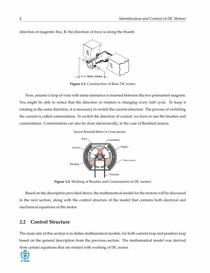
direction of magentic flux, B, the direction of force is along the thumb.
Figure 2.1: Construction of Basic DC motor
Now, assume a loop of wire with some resistance is inserted between the two permanent magnets.
You might be able to notice that the direction of rotation is changing every half cycle. To keep it
rotating in the same direction, it is necessary to switch the current direction. The process of switching
the current is called commutation. To switch the direction of current, we have to use the brushes and
commutators. Commutation can also be done electronically, in the case of Brushed motors.
Figure 2.2: Working of Brushes and Commutators in DC motors
Based on the description provided above, the mathematical model for the motors will be discussed
in the next section, along with the control structure of the model that contains both electrical and
mechanical equations of the motor.
2.2 Control Structure
The main aim of this section is to define mathematical models, for both current loop and position loop
based on the general description from the previous section. The mathematical model was derived
from certain equations that are related with working of DC motor.
Page 10
Identification and Control of DC Motors 5
A mathematical model is a description of a system using mathematical concepts and language.
Mathematical models, in general, can take many forms including dynamic systems, differential equa-
tions, statistical models, etc. In this case, the goal is to develop the mathematical model for Dynamic
system which relates the voltage applied to the armature to the position of the motor.
The set of equations that will be described later in the following subsections, may be represented
as nonlinear dynamic system. The main restrictions of this model, with respect to a real motor are
• Assumption that the magnetic circuit is linear
• Assumption that the mechanical friction is only linear in the motor speed.
These restrictions are considered in the identification of the model and based on the restrictions,
equations have been derived.
2.2.1 Electrical Characteristics
The most important part in this section is the physical reasoning behind the concept of transforming
electrical power in mechanical power. As a matter of fact, since the magnetic field B arises from the
stator coils, not only the rotor coils may rotate with respect to the stator, but also the stator supply may
rotate by increasing the number of coils and by a more sophisticated way. The equivalent electrical
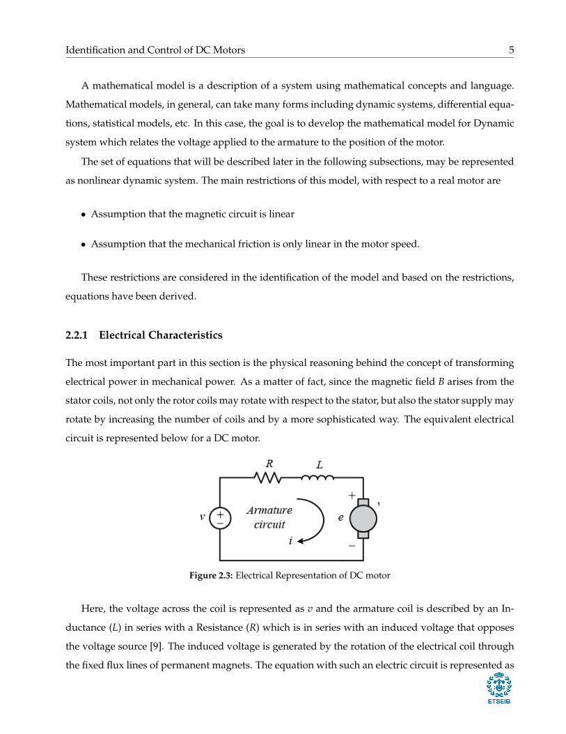
circuit is represented below for a DC motor.
Figure 2.3: Electrical Representation of DC motor
Here, the voltage across the coil is represented as v and the armature coil is described by an In-
ductance (L) in series with a Resistance (R) which is in series with an induced voltage that opposes
the voltage source [9]. The induced voltage is generated by the rotation of the electrical coil through
the fixed flux lines of permanent magnets. The equation with such an electric circuit is represented as
Page 11
6 Identification and Control of DC Motors
v(t) = Ldidt
+ Ri (2.1)
Since, the (Eq. 2.1) was assumed to be linear, using the Laplace transform as shown in (Eq. 2.2)
we can obtain the transfer function between current and voltage [9].
i(s)v(s)
=K
τs + 1(2.2)
where K = 1R is the stator gain and τ = L
R is the stator time constant.
Based on the above derivation, we can further deduce the relation between current and torque.
For DC motor, Torque is considered as the electromagnetic torque and it varies only with flux φ and
the current I as follows
T = k ∗ φ ∗ I (2.3)
2.2.2 Mechanical Characterstics
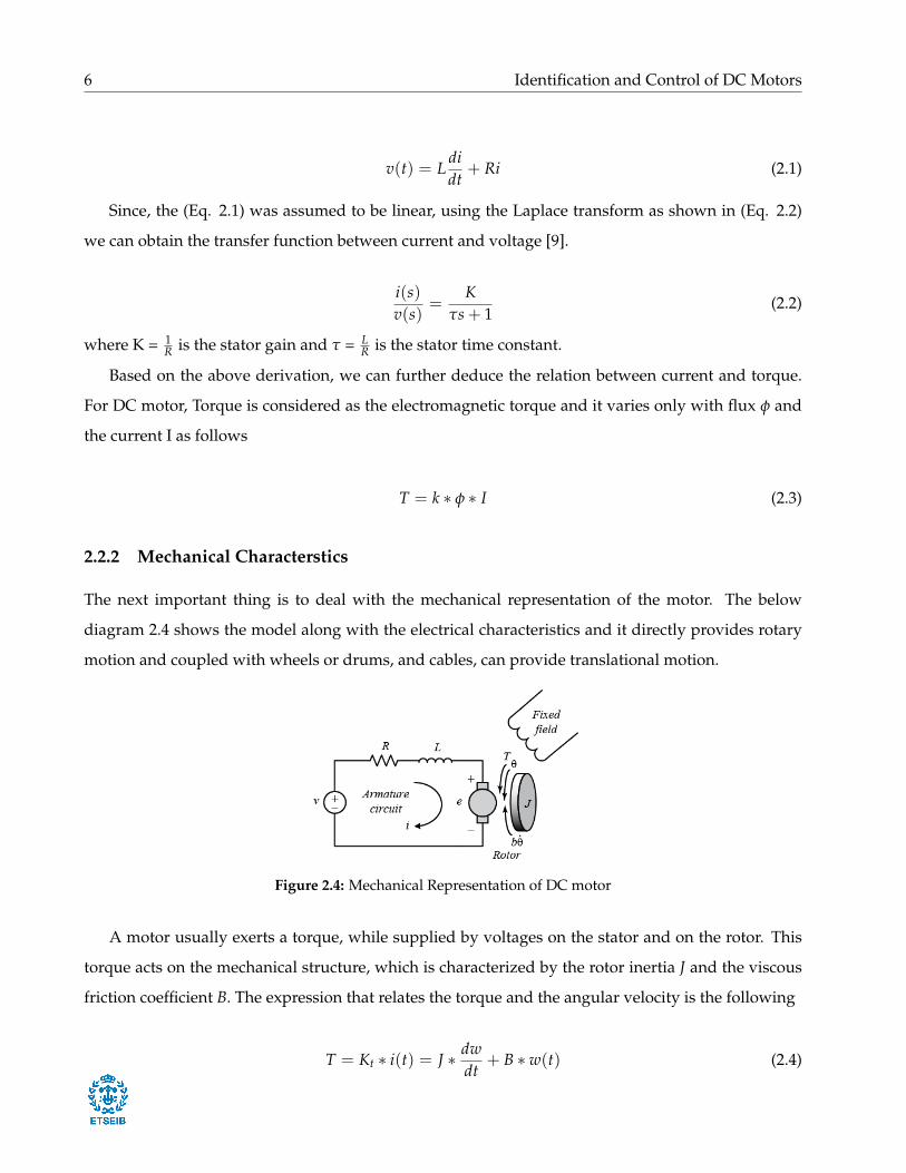
The next important thing is to deal with the mechanical representation of the motor. The below
diagram 2.4 shows the model along with the electrical characteristics and it directly provides rotary
motion and coupled with wheels or drums, and cables, can provide translational motion.
Figure 2.4: Mechanical Representation of DC motor
A motor usually exerts a torque, while supplied by voltages on the stator and on the rotor. This
torque acts on the mechanical structure, which is characterized by the rotor inertia J and the viscous
friction coefficient B. The expression that relates the torque and the angular velocity is the following
T = Kt ∗ i(t) = J ∗ dwdt
+ B ∗ w(t) (2.4)
Page 12
Identification and Control of DC Motors 7
where Kt is the torque constant which relates the current through the torque generated as shown in
the article [3]. Since, the velocity of the motor can further deduced into position as follows
w(t) =dθ(t)
dt(2.5)
Substituting the (Eq. 2.5) into (Eq. 2.4), it gives
Kt ∗ i(t) = J ∗ d2θ(t)dt2 + B ∗ dθ(t)
dt(2.6)
Applying Laplace transformation to the (Eq. 2.6),
Kt ∗ i(s) = J ∗ θ(s) ∗ s2 + B ∗ θ(s) ∗ s (2.7)
The mechanical model of the motor Gmotor is defined between the position θ(s) and the current i(s)
Gmotor =θ(s)i(s)
=KtB
s ∗ ( JB s + 1)
(2.8)
And this expression can be changed by replacing the terms of Kt, J andB. Assuming that there is no
such values, as manufacturers typically do not provide, must also take into account the own inertia of
the load coupled to the motor shaft; its effect can be modeled as a disturbance on the system, which
must be corrected by the control loop. Therefore, it ignores these physical parameters and transforms
the physical model in a control-oriented model, being
Gmotor,pos =k
s(τs + 1)(2.9)
The above (Eq. 2.9) represents the model of the position loop and the velocity model can be
reduced to by just removing the integrator from the above model being represented as follows
Gmotor,vel =k
(τs + 1)(2.10)
2.3 Control Law
Control theory is an interdisciplinary branch of engineering and mathematics that deals with the be-
haviour of dynamical systems with inputs, and how their behaviour is modified by feedback. The
usual objective of the control theory is to control a plant, which gives an output that follows a control
Page 13
8 Identification and Control of DC Motors
signal called reference, which maybe a fixed or changing value. For this, it is necessary to design
a controller to monitor the output comparing it with the reference. The difference between the ac-
tual and desired output, called an error signal, is applied as feedback to the input of the system, to
bring the actual output closer to the reference. A block diagram representing the control thoery is
represented below in the Figure 2.5.
Figure 2.5: Block diagram representation of negative feedback control system
Figure 2.6: Block diagram representation of single-input single-output (SISO) system
In general, the Figure 2.6 represents linear and time-invariant system where C is the controller,
P is the plant and F is the feedback of the system. The system can be analysed using the Laplace
transform on the variables and thus, give the following relations:
Y(s) = P(s)U(s) (2.11a)
U(s) = C(s)E(s) (2.11b)
E(s) = R(s)− F(s)Y(s) (2.11c)
And now solving for Y(s) in terms of R(s), we get
Y(s) =P(s)C(s)
1 + F(s)P(s)C(s)R(s) = H(s)R(s) (2.12)
This is called the Closed-loop transfer function and in most of the case, F(s) = 1. Using the above
transfer function method in motor control, it will be a way of designing the controller to achieve and
Page 14
Identification and Control of DC Motors 9
maintain a goal state by constantly comparing current state with goal state. And the feedback in this
case, is given from a sensor feedback. And, the PID controller with or without view modifications is
the most common controller used in the servo drives of the motor. For electrical characteristics of the
motor, the PI controller was used to make the model stabilize and for the position or velocity loop,
PID controller is used as explained in the following sections.
2.3.1 PI controller
The Proportional-Integral (PI) algorithm computes and transmits a controller output signal every
sample time, Ts. PI controller has two tuning parameters to adjust. Integral action enables PI con-
troller to eliminate offset, in case the open loop plant does not contain any integrator, which is a ma-
jor weakness of P-only controller. Thus, PI controllers provide complexity and capability that makes
them by far the most widely used algorithm in process control algorithms.
The controller output is given by
Kpe(t) + Ki
∫e(t)dt (2.13)
where e(t) is the error of deviation of actual measured value from the setpoint.
The lack of derivative action may make the system more steady in the steady state in the case of
noisy data. And this type of controller is used to control the current flow in the motors.
2.3.2 PID controller
The PID (Proportional-Integral-Derivative) controller is a control loop feedback mechanism which is
commonly used in the industrial systems. It continuously calculates an error value as the difference
between a desired setpoint and a measured process variable. The controller attempts to minimize the
error over time by adjustment of a control variable to a new value determined by a weighted sum:
u(t) = Kpe(t) + Ki
∫ t
0e(τ)dτ + Kd
de(t)dt
(2.14)
where Kp, Ki and Kd denote non-negative coefficients for the proportional, integral and derivative
terms respectively.
Page 15
10 Identification and Control of DC Motors
Figure 2.7: Block diagram of a PID controller in a feedback loop
Designing PID controller
In the control of DC motors, a standard specification is based on specifying the bandwidth. This can
be by specifying the closed loops through the following procedure:
• Find the transfer function of the system, and express it in terms of the variable s from the Laplace
transform, if applicable
• Convert s→ jω
• Find the magnitude of the expression obtained in the previous point
• Equal expression of the first magnitude 1√2, obtained for the case ω = ωBW and solve the result-
ing equation to find ωBW
As mentioned above, chosen the system presents a unique closed loop pole with multiplicity three.
The most general is
Gdesired =1
(τs + 1)3 (2.15)
Substituting the conversion of s→ Jω, we get
Gdesired =1
(τ jω + 1)3 (2.16)
Now, the magnitude of the Gdesired is,
Gdesired =1
[√
τ2ω2 + 1]3(2.17)
Page 16
Identification and Control of DC Motors 11
Equating (Eq. 2.17) to 1√2
for ω = ωBW ,
1[√
τ2ω2 + 1]3=
1√2
(2.18)
For a simple transfer function of first order model, the poles are:
pol = − 1τ
(2.19)
Substituting the (Eq. 2.19) in (Eq. 2.18), we get
1
[√
ω2
pol2 + 1]3=
1√2
(2.20)
From the equation (Eq. 2.20), we can determine the pol as
pol = ± ωBW√3√
2− 1(2.21)
To make the system stable, the poles are placed on the left half plane and thus,
pol = − ωBW√3√
2− 1(2.22)
Using this above definition of the poles, we can determine the controller gains as discussed in the
following chapters.
Page 17
Chapter 3
Real Setup
In this chapter, we will be concentrating on the description of the softwares and the equipments
used throughout the project. It shows the systems used in this project, the servo drives, the feedback
and the software used to make the system activate. We will also be discussing about the company
requirements that they can depend on the project to improve their software.
The main important requirements from the company is to design and identify the model of the
motor, collecting data from the software MOTIONLAB and applying it in MATLAB software, where
we experiment on the system that will be discussed in the next chapter. MOTIONLAB software is
the platform in which all the company’s products help improve the system based on the customer
requirements. It has various applications that let us configure, program, test and run the drive in
a way that are intuitive and simple. And using the features in the software, a tool was designed
to determine the data of the motor for the identification of the system. Below Figure 3.1 shows the
MOTIONLAB configuration window where the firmware of the identification is uploaded and the
identification tool is activated, as seen in the Figure 3.2.
Motors have various applications in the real world, like it can be used in vehicles, cranes, air
compressors, conveyors and machines like Weaving machine, Lathe machines, etc. And one of the
main applications, that is currently the present and future of science and technology, are the study
of Robotics. Motors are generally the motion part of the robots as it is defined in the Section 2.1. In
this case, the brushed DC motors are used provided by the company Ingenia Motion Control, namely,
Mot 37 and Mot 53 as shown in the Figures 3.3 and 3.4 respectively.
12
Page 18
Identification and Control of DC Motors 13
Figure 3.1: MotionLab Configuration Window
Figure 3.2: Identification Tool to collect the datas from the motor
Figure 3.3: Motor Mot 37
Page 19
14 Identification and Control of DC Motors
Figure 3.4: Motor Mot 53
The next important part required for this project is the servo drive which acts the communication
channel between the motor and the computer. The company provided one of their main servo drive
called Pluto Digital Servo Drive, which is shown in the below Figure 3.6. This servo drive is the
modular solution for control of rotary or linear brushed DC motors, that works up to 800 W peak,
with 8 A continuous output current and no heat sink needed. The controller in the Pluto includes
two control loops: one of them made from an electrical point of view - Current; and the other, from
a mechanical point of view - Position. Although only mentioned that the work focuses on the bond
position, it is considered interesting to show how the two are related ties. Figure 3.5 below shows the
connection between these two loops and other elements that make up the system study:
Figure 3.5: Block Diagram of the Control Structure of the Pluto
Page 20
Identification and Control of DC Motors 15
Figure 3.6: Pluto Digital Servo drive
Figure 3.7: Setup of the Motor 37
Figure 3.8: Setup of the Motor 53
Page 21
16 Identification and Control of DC Motors
Finally, the last thing needed for the setup of the project is a feedback and a battery supply. Each
motor has their own specifications with their own values provided by the manufacturer. The motors
that are in use in this project needs a 24 Volts power supply to make the servo drive active, where
the data sheet is presented in the Appendix A. And the feedback used here, is a Digital Encoder,
for velocity control and/or position control as well as commutation sensor. The encoder provides
incremental position feedback that can be extrapolated into precise velocity or position information.
Page 22
Chapter 4
System Identification
This chapter is structured as follows: firstly, the design of input disturbances for the identification,
secondly, the analysis of model structures and finally, the electrical identification and the mechanical
identification of the motors.
4.1 Design of Inputs
This section deals with the input disturbance signal which is the basis for the system identification of
both electrical and mechanical part of the motor.
In general, the output can be exactly calculated once the input is known and in most of the cases,
this looks unrealistic. Thus, we need some form of disturbances that can be considered as input for
a system. Based on these inputs, we calculate the output and use this for identification. And the
most important thing here, is to design the input signals. These signals can be either a Sine Sweep, a
Psuedo-Random binary noise or a Multisine. And in this case, Multisinus is considered as the natural
choice of input, that can be seen in [8], which can be formed as sum of sinusoids
u(t) =d
∑k=1
akcos(wkt + ϕk) (4.1)
ϕk ,−k.(k− 1).π
N(4.2)
wk , wmin +(k− 1).(wmax − wmin)
N(4.3)
where ak is the amplitude, wk is the frequency in rad/s and ϕ is the phase angle.
17
Page 23
18 Identification and Control of DC Motors
wmax = 2π fmax; wmin = 2π fmin
With the above parameters ak and wk, we can place the signal power very precisely to desired
frequencies.
The signal chosen obtains a combination of sinusoidal signals - called Multisinus from now -
which covers the frequency spectrum needed for the study.
A specific frequency range has to be mentioned that is required for the operation MATLAB func-
tion msinclip2 used for generating the multisinus. In essence, the operation iterates towards a set of
phases to solve the problem of the crest factor, where the algorithm was presented to minimize the
peaks of the band limited Fourier signals. This method has the ability to compress the signals effec-
tively without disturbing the spectral magnitudes. The result of this operation is a vector of complex
amplitudes of multisinus, which are calculated on a series of operations that lead to the final vector
of input values. This entry is to be used to calculate the output.
One of the most important property of this signal is that there is no leakage and thus the periodic
signal has a period of T0 = 1/ f0. And the crest factor typically used is 1.7 and we use smaller crest
factors to optimize the phases using a numerical optimization routine. These signals can be calculated
using Fourier Transformation as mentioned above.
The following sections talks about the frequency resolution and the properties of the signal for
Current loop and Position loop respectively.
4.1.1 Current Loop
The current loop works with a sampling frequency 10kHz So, the input signal should have a fre-
quency limit of 5kHz and if it goes past this limit, the model unstable and thus we can use the maxi-
mum frequency for the identification as 4kHz.
In this case, we can use a lower frequency for the identification but for the current loop, the motor
should not move. It is because higher frequency has a lower time constant as it frequency is indirectly
proportional to time constant. So, identification is done for the maximum frequency f=4000 Hz and
the plot of amplitude vs time is shown in Figure 4.1. Whereas, for the low frequency, the electrical
time constant is high enough for the motor to move back and forth as shown in Figure 4.2.
The identification of electrical model is done in both open loop and closed loop to see which
provides a better solution, which will be discussed further in the identification of the current loop.
Page 24
Identification and Control of DC Motors 19
Figure 4.1: Multisinus input with frequency f = 4kHz
Figure 4.2: Multisinus input with frequency f = 100 Hz
For open loop identification, the percentage of amplitude is given as 50% which is common for all the
motors because the input is the signal injected and for certain motors, the current flow throughout
the model may affect the system and it will be a little difficult to identify the electrical model. The
disturbance is measured as percentage of duty cycle and each duty has a maximum limit as follows
MaxDuty = 100.MotorRatedcurrent.MotorResistance
Voltage(4.4)
For closed loop identification, the percentage of amplitude is given as 10% as the closed loop
identification has an offset as the input. This type of identification also involves a controller and
the disturbance is added after the controller as described in the later part of this chapter. Here, the
disturbance is measured in terms of % of rated torque which can be converted into milli-Newton
using the (Eq. 4.5).
Torque(mN) =Torque(%).RatedTorque(mN)
1000(4.5)
Page 25
20 Identification and Control of DC Motors
4.1.2 Position Loop
In this section, the main aim is to determine the disturbance signal for the mechanical characteristics
of the motor. The position loop works with a sampling frequency of 1 kHz. In this case, the maximum
frequency input is 400Hz which is the maximum input for the system identification.
Here, the frequency injected can be of any range that corresponds to the motor requirements and
the frequency resolution. Since the maximum frequency that can be injected is 400 Hz, the experiment
begins with f = 400 Hz as shown in Figure 4.3.
Figure 4.3: Multisinus input with frequency f = 400 Hz
For the identification of the position loop, the motor needs to move a step for the identification to
be possible, which will be discussed later in this chapter. And thus, the mechanical time constant does
not directly depend on the disturbance injected and thus, the frequency can be varied for identifying
the model. In this case, the frequencies used are f = 100 Hz and f = 200 Hz apart from the maximum
frequency input as shown in Figures 4.4 and 4.5.
Figure 4.4: Multisinus input with frequency f = 200 Hz
Since, the identification can only be done in closed loop for position loop, we set an amplitude for
Page 26
Identification and Control of DC Motors 21
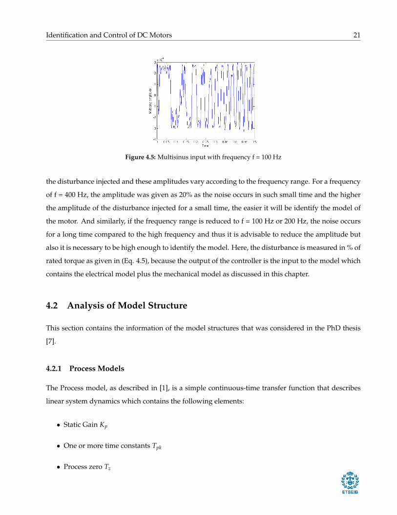
Figure 4.5: Multisinus input with frequency f = 100 Hz
the disturbance injected and these amplitudes vary according to the frequency range. For a frequency
of f = 400 Hz, the amplitude was given as 20% as the noise occurs in such small time and the higher
the amplitude of the disturbance injected for a small time, the easier it will be identify the model of
the motor. And similarly, if the frequency range is reduced to f = 100 Hz or 200 Hz, the noise occurs
for a long time compared to the high frequency and thus it is advisable to reduce the amplitude but
also it is necessary to be high enough to identify the model. Here, the disturbance is measured in % of
rated torque as given in (Eq. 4.5), because the output of the controller is the input to the model which
contains the electrical model plus the mechanical model as discussed in this chapter.
4.2 Analysis of Model Structure
This section contains the information of the model structures that was considered in the PhD thesis
[7].
4.2.1 Process Models
The Process model, as described in [1], is a simple continuous-time transfer function that describes
linear system dynamics which contains the following elements:
• Static Gain Kp
• One or more time constants Tpk
• Process zero Tz
Page 27
22 Identification and Control of DC Motors
The above elements describe specifically the system dynamics that can be used for the identifica-
tion. The advantages of the model are that they are simple and the model coefficients have an easy
interpretation as poles and zeros. There is a possibility to create different model structures by varying
the poles, adding an integrator, add a time delay or add a zero. But in this case, the model we describe
is either a first order model or first order plus integrator model refer to the motor models presented
in the previous chapter.
G(s) =Kp
τp1s + 1(4.6)
G(s) =Kp
s(τp1s + 1)(4.7)
where Kp is the static gain and τp1 is the time constant.
4.2.2 Polynomial model
A polynomial model uses a generalized notion of transfer functions to express the relationship be-
tween the input u(t), the output y(t) and the noise e(t) using the equation:
A(q)y(t) =nu
∑i=1
Bi(q)Fi(q)
ui(t− nki) +C(q)D(q)
e(t) (4.8)
The variables A,B,C,D,F are the polynomials expressed in the time shift operator q−1, ui is the input
at i, nu is the total number of inputs, and nki is the input delay. There are different configurations of
polynomial models and those are represented in the following subsections [2].
ARX Model
The ARX model (Auto regressive with exogenous terms) is the simplest model that incorporates the
stimulus signal. However, this model captures some of the stochastic dynamics as part of the system
dynamics. This model is the easiest to estimate since the corresponding estimation problem is of a
linear regression type.
A(z)y(k) = B(z)u(k− n) + e(k) (4.9)
where the u(k) is system inputs, y(k) is system outputs, n is system delay and e(k) is system distur-
bance.
Page 28
Identification and Control of DC Motors 23
A(z) and B(z) are polynomial with respect to backward shift operator z−1 and defined by the
following
A(z) = 1 + a1z−1 + a2z−2 + ... + aka z−ka (4.10)
B(z) = b0 + b1z−1 + ... + akb−1z−(kb−1) (4.11)
The identification method of the ARX model is the least squares method, which is special case
of the prediction error method.The least squares method is the most efficient polynomial estimation
method because this method solves linear regression equations in analytic form and the solution is
unique. The foremost disadvantage is that the disturbance model comes along with the system poles
and this makes it easier to get an incorrect estimate of the system dynamics because the polynomial
A can also include the disturbance properties.
OE model
The general linear polynomial model reduces to the output-error model. This model describes the
system dynamics separately from the system dynamics. The output-error model does not use any
parameters for simulating the disturbance characteristics. The following equation shows the form of
the output error model:
y(k) =B(z)F(z)
u(k− n) + e(k) (4.12)
where the u(k) is system inputs, y(k) is system outputs, n is system delay and e(k) is system distur-
bance.
B(z) and F(z) are polynomial with respect to backward shift operator z−1 and defined by the
following equations.
B(z) = b0 + b1z−1 + ... + akb−1z−(kb−1) (4.13)
F(z) = 1 + f1z−1 + f2z−2 + ... + ak f z−k f (4.14)
The identification method of the output error model is the prediction error method, which is quite
similar to ARMAX model structure. If the disturbance e(k) is white noise, all minima are global.
However, a local minimum can exist if the disturbance is not white noise.
Page 29
24 Identification and Control of DC Motors
Conclusion on the Model Structure
From this section, the process model structure was used for the identification of both current loop
and position loop as the order of the model was easy to predict and the identification of the system
works better with continuous time than discrete system which will be discussed in the results later in
the chapter. The reason to neglect ARX model is because the identified model is actually a predicted
model that does not depend directly on the input and output, which might cause some trouble in
designing the controller.
4.3 Identification methods
This section deals with the concept of System identification for electrical and mechanical loops of the
motor. It involves the technique used for injecting the disturbance, analysis of model structures in
continuous time and in discrete time, and the representation of mathematical models along with the
results.
In general, each object begins and ends with a real data and analysing the data will provide with
no desire to move forward in the field of Control systems. And thus, the concept of System Identifi-
cation can be presented as discussed in the book [4]. System Identification uses statistical methods to
build mathematical models from the measured data. The process of converting the data into mathe-
matical models are fundamental in the field of science and engineering and is one of the crucial topics
in the Control systems area.
System identification has been an active research area for the past two decades and it has now ma-
tured and many techniques have been standardized in the control and signal processing engineering.
It also includes the optimal design of experiments to efficiently generate informative data for fitting
models as well as model reduction. It is characterized into three categories:
• White-box: It estimates the parameters of the physical model from data
• Grey-box: Using a generic model structure, estimate the parameters from data
• Black-box: Determine model structure and estimate the parameters from data
In general, most of the systems are considered as Black-box models as the only known factors are
the real data obtained. It is necessary to analyse various model structures to get a better fit from the
Page 30
Identification and Control of DC Motors 25
measured data and there are many types of model structures that have been become standard tools in
the MATLAB. Using the analysis of model structures from the previous section, the model can be in
continuous time and the model structure we can chose is process model as it gives a better fit which
will be discussed in the following sections.
4.3.1 Electrical Identification
The electrical characteristics of the model was discussed in the previous Chapter 2 and the model is
described in the Section 2.2.1 in the (Eq. 2.2) which describes the first order model for the current
loop, that contains the variables Inductance (L) and Resistance (R).
But, there are two methods for identifying the electrical model of the motor and those are:
• Open Loop Identification
• Closed Loop Identification
Both the methods will be discussed in the coming sections along with the results in both time
domain and frequency domain.
Open loop method
The Open Loop identification method is the simplest and easiest method for the identification of any
model. Theoretically, the identification of the model is done between the reference and the Actual
output of the real system and a disturbance is applied after the controller to make the system react
and then identify the model. This representation is shown in Figure 4.6. In most of the cases, the input
is not known and thus it will be difficult to calculate the output of the system. Thus, we use signals
that are under our control and determine the output of the system. There are signals that are beyond
our control that also affect the system but within our linear framework, we assume to be negligible.
Here, the reference is not known and thus the disturbance is designed as mentioned in the previous
section and the model was further reduced as shown in Figure 4.7.
The above method was introduced in the MOTIONLAB Identification tool software and the mul-
tisinus was introduced with a certain amount of amplitude and applied in the motors which were
discussed in the previous Chapter 3.
The amplitude of the signal injected is important for the systems to identify the model. Some
systems might not be able to take 100% amplitude and also for safety reasons, we apply 50% signal
Page 31
26 Identification and Control of DC Motors
Figure 4.6: Open loop System from Reference (Demand) to Output (Actual)
Figure 4.7: Open loop System from Disturbance to Output (Actual) reduced from Figure 4.6
amplitude of the Multisinus. As the input signal is injected, the motor gives a small reaction which
shows that the motor responds to the input signal. Then the output of the model is taken from
software and exported to the MATLAB.
Using the input and output of the system, the model can be identified using the System Identi-
fication Application from the MATLAB software. Here, the sampling time given to be Ts = 0.0001
seconds.
The next step is to choose the model structure of the system. The easiest way to choose the model
structure to identify the model in continuous and later convert it into discrete. And thus, the model
structure used here is Process model as described in the previous chapters, which contains a gain and
a first order pole as shown in (Eq.4.16). Initially, the main idea of the identification is to match the pa-
rameters of the motor with the values contained in datasheets. But due to lack of certain information
such as the model of the servo drive, the matching of parameters could not be done and the next best
option was to look for the better fit model.
The fitting of the model is done in both Time domain and Frequency domain. Since it is easier to
work in continuous time, the model structure was chosen to be Process model. The fit and the Bode
plot for the motors Mot 37 and Mot 53 are shown in the later subsections.
Based on this, the parameters can be extracted from the model along with the frequency domain
fit of the model. The frequency domain plot is produced to show the data estimation of the model, i.e.,
the input and output was converted in the Fast Fourier Transform (FFT). The conversion was done
Page 32
Identification and Control of DC Motors 27
with the function fft in MATLAB, which gives the input and output in the frequency domain and the
fit of the model is found.
The parameters of the model are represented as mentioned in the (Eq. 4.16), which can be used for
further use for designing of the controller. This model was further used for verification by injecting a
small step and it was also verified with the Bode diagram of the system.
The Bode plot contains the transfer function using the above parameters which is in continuous
time and the transfer function was also converted into Discrete time. It also contains the data estima-
tion of the input and output in frequency domain which was done with a function tdf in MATLAB.
This function gives the magnitudes and phases of the input and output based on different input fre-
quencies.
The model works better with higher frequencies because the electrical time constant is too small,
whereas for the lower frequencies, the estimated input and output frequencies does not even come
close to the transfer function. And as the input frequency is higher, it matches well with the gain
margin of the transfer function. The identification is done in time domain and later converted to
frequency domain such that Bode plots show the gain margin required to maintain stability under
variations in circuit characteristics caused during manufacture or during operation. And comparing
the other model structures with process model structure, the identified model using process model
provides a better fit, although Output error model structure came a little close as it depends on the
input and output data unlike ARX model which is based on prediction of the output.
Page 33
28 Identification and Control of DC Motors
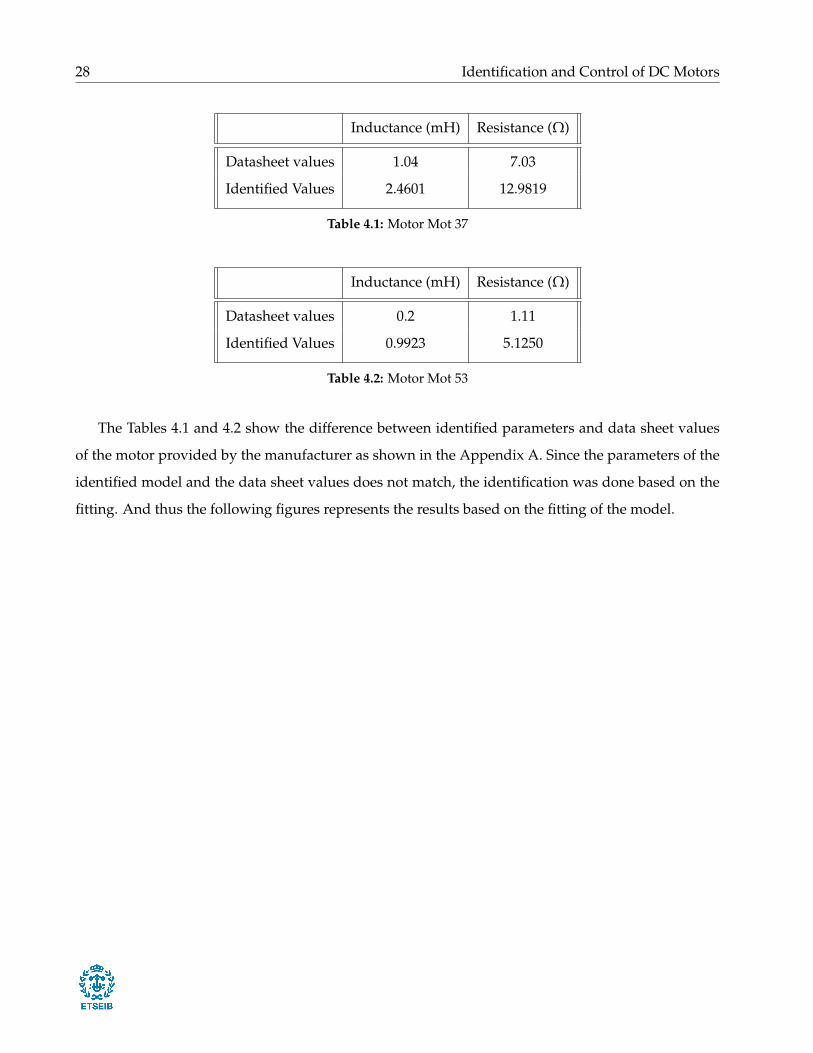
Inductance (mH) Resistance (Ω)
Datasheet values 1.04 7.03
Identified Values 2.4601 12.9819
Table 4.1: Motor Mot 37
Inductance (mH) Resistance (Ω)
Datasheet values 0.2 1.11
Identified Values 0.9923 5.1250
Table 4.2: Motor Mot 53
The Tables 4.1 and 4.2 show the difference between identified parameters and data sheet values
of the motor provided by the manufacturer as shown in the Appendix A. Since the parameters of the
identified model and the data sheet values does not match, the identification was done based on the
fitting. And thus the following figures represents the results based on the fitting of the model.
Page 34
Identification and Control of DC Motors 29
MOT 37:
Best Fit of the model
Figure 4.8: Fit of the electrical model in Time Domain using System Identification tool
Bode Plot
Figure 4.9: Bode plot of the motor MOT 37
Transfer function of the electrical part of the motor is:
G(s) =0.0770
1.895e− 04s + 1(4.15)
Page 35
30 Identification and Control of DC Motors
MOT 53:
Best Fit of the model
Figure 4.10: Fit of the electrical model in Time Domain using System Identification tool
Bode Plot
Figure 4.11: Bode plot of the motor MOT 53
Transfer function of the electrical part of the motor is:
G(s) =0.1951
1.9363e− 04s + 1(4.16)
Page 36
Identification and Control of DC Motors 31
Closed loop method
There are several schemes for plant model identification in closed-loop operation including classical
direct method, step identification and closed-loop output error algorithms are considered. These
methods are analyzed and compared in terms of the bias distribution of the estimates for the case that
the noise model is estimated as well as the case that a fixed model of noise is considered. But for the
electrical characteristics, the closed-loop operation cannot be succeeded because the motor should not
move as described in the previous chapters. And thus, for the closed-loop identification, the motor
moves as the motor gives a step input as well as the noise, in this case, a multisinus.
Conclusions on the Electrical Identification
As already discussed above, the open loop identification for the electrical identification seems feasible
as the closed loop identification provides information which does not identify the model of the cur-
rent loop. Closed loop identification makes the system moves which allows the system identification
for the position loop rather than torque loop, and thus, the closed loop identification cannot used for
the identification of the electrical characteristics of the motor. For the open loop identification, the in-
ductance and resistance does not provide the exact values of the motor provided by the manufacturer
as the system might detect not only the current loop but also some effect from the outside which is
very difficult to predict. But the bode plot of the open loop identification provides a better solution
as the data estimated from the multisinus input matches the bode plot of the transfer function, thus
making the open loop identification more effective.
4.3.2 Mechanical Identification
Once the file containing the values of the variables for current loop is recorded, the identification
model engine starts properly. This identification will be carried out following two different methods:
first, use the identification toolbox of visual character; on the other, it follows the process model
method. This course of action has a dual aim: first, they can directly compare the results for each
method so that you can know whether or not they are consistent; it is also a way to meet several
alternatives when adjusted models.
Page 37
32 Identification and Control of DC Motors
Identification ToolBox
The identification of MATLAB toolbox is a tool that allows for the mathematical model that best
represents a data set intuitively. This operation is carried out in three stages:
Import data: reads the parameters previously recorded file on the MATLAB. In this case, select
the option Time domain data, as the data come from a real experiment.
Estimate: computes the proper identification model. There are various types of estimate, accord-
ing to the way they want to get the model: in the form of state space or as a transfer function as a
polynomial model, etc. In this case, we opt for a process model; that is, a continuous-time transfer
function that describes the dynamics of a linear system as explained in the previous chapter. This
transfer function is characterized by means of a series of parameters. The selection of model and
other parameters, as well as its multiplicity, the model obtained will be different in each case.
And in this case, since the current loop and position loop works on different frequency, the model
of the current loop is considered to be in the position loop as a gain. But, the controller of the current
loop needs to be designed before the identification of the position loop because a steady current
flowing through the position loop makes the system stable. And the next thing to concentrate on how
to determine the data and record them using the closed-loop techniques.
Closed-loop method
This section deals with the identification techniques such as open loop and closed loop method and
it is necessary how the techniques has been applied and which are the inputs used in this technique.
As for open loop method for the mechanical identification, the motor does not move as there is no
feedback for the motor output. For the identification of the mechanical model to work, the motor
needs to move and this does not happen in open loop, so this technique cannot be used in the position
loop.
The closed-loop method is the best way to move the motor and further determine the input and
output of the model, analyse and using this data, identify the model of the motor. In this case, the
method involves two inputs, namely, step input and the disturbance input for the motor as explained
in the Section 4.1. This method also comes along with the proportional controller to make the motor
move for the identification as shown in the figure 4.12.
The block diagram representation can further be reduced to determine the model of the motor
in a easier and simpler way. The closed-loop block diagram is represented below in the figure 4.13.
Page 38
Identification and Control of DC Motors 33
Figure 4.12: Closed-loop block diagram of the Mechanical model
As shown in the figure, the input is described as combination of step input and the proportional
controller(Kp) and added to the disturbance of the model as follows
u = StepInput ∗ Kp + Disturbance (4.17)
Figure 4.13: Reduced Closed-loop block diagram of the Mechanical model
In the MotionLab software, the reduced model was applied but the values are inserted for step
input and disturbance input signal and the software automatically converts the two inputs into one.
As the motor moves and the output is recorded, both input and output of the reduced model is
exported into MATLAB for further analysis and the identification of the model.
Here, the output data is further reduced by removing the integrator since the identification of the
model will be difficult using the current output. Thus, the derivative of the current output is used
instead.
NewOutput(k) =Output(k)−Output(k− 1)
Ts(4.18)
Page 39
34 Identification and Control of DC Motors
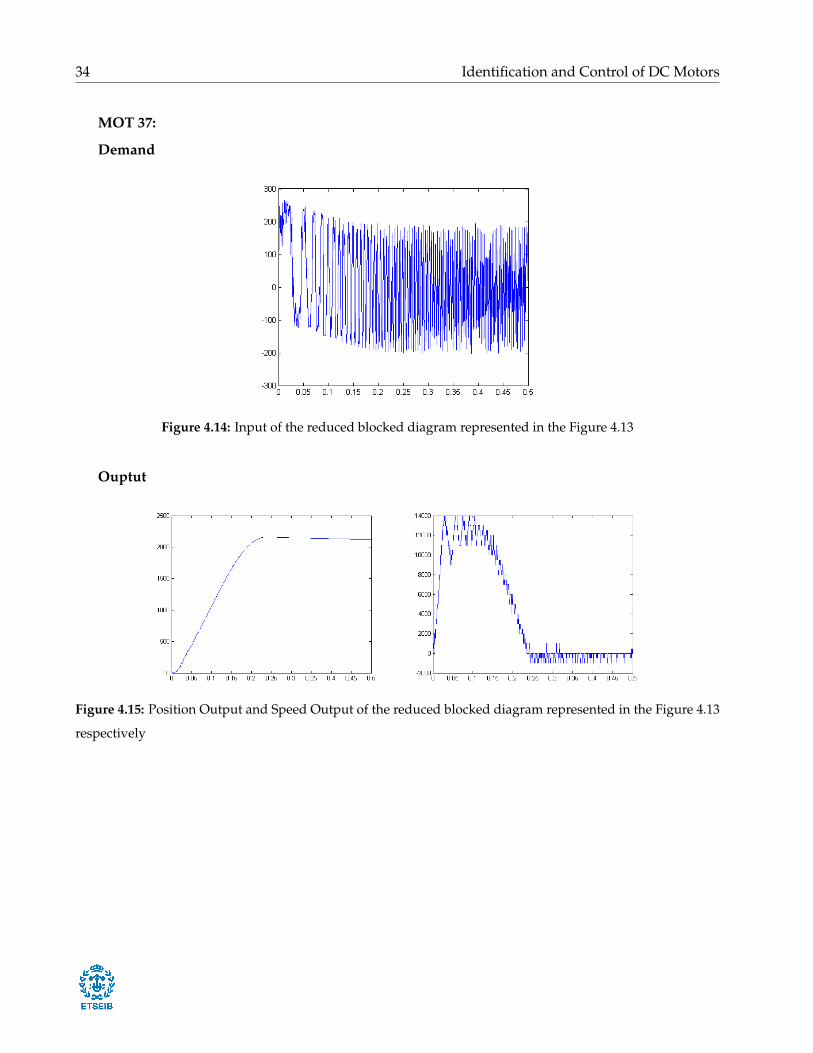
MOT 37:
Demand
Figure 4.14: Input of the reduced blocked diagram represented in the Figure 4.13
Ouptut
Figure 4.15: Position Output and Speed Output of the reduced blocked diagram represented in the Figure 4.13
respectively
Page 40
Identification and Control of DC Motors 35
MOT 53:
Demand
Figure 4.16: Input of the reduced blocked diagram represented in the Figure 4.13
Ouptut
Figure 4.17: Position Output and Speed Output of the reduced blocked diagram represented in the Figure 4.13
respectively
Page 41
36 Identification and Control of DC Motors
This new output will be defined as a velocity output and thus the identified model will be a ve-
locity model. The next section deals with the further analysis of data estimated using the frequency
response of both the DC motors which presents various step inputs for different disturbance fre-
quency.
Analysis of Data estimation
In this section, the main aim is to discuss the frequency response of the data estimated from the model
from the previous subsection. The data estimated are, in general, the input and output of the system.
As explained in the previous section, the input of the system is the combination of proportional con-
troller and step input added with the disturbance as shown in the (Eq. 4.17). The output, as discussed
in the previous subsection, is taken as the speed of the motor. And also, using the analysis of the data
estimated, the model has been identified using the process model structure along with the results.
The main aim of this topic is to analyse the input of the reduced block diagram shown in Figure
4.13 because as the input varies, the frequency response also varies. The relation between the step
input, disturbance signal and the proportional controller is the most important concept that will be
dealt for the data estimation. And also, the disturbance signal can be of any frequency and in this
case, the frequency injected for the disturbance signal is described as in the Section 4.1.
In the case of rotary motors, the size of the step does not have any limits on the step input. As
explained in the previous Chapter 3, the step input is in counts and the input used are 2000c, 3000c
and 4000c. The disturbance signal injected have a frequency of 100 Hz, 200 Hz and 400 Hz. This
signal should not be injected at full amplitude as the motor will become unstable and it will be very
difficult to identify the model. So, the amplitude of signal injected is approximately 10-20% as that
would suffice for the identification of the mechanical model.
Now, the relation between the input and the proportional controller is very important in this case.
For a higher step input, the less the proportional controller should be. As shown in the figures of
the analysis shown below, there are few peaks which can be considered as the instability in the data
estimation but it can be misinterpreted as the resonance.
Page 42
Identification and Control of DC Motors 37
MOT 37:
Figure 4.18: Data estimation for Step size = 2000c and Disturbance signal = 400 Hz with Kp = 2000
Figure 4.19: Data estimation for Step size = 2000c and Disturbance signal = 400 Hz with Kp = 3500
Figure 4.20: Data estimation for Step size = 2000c and Disturbance signal = 400 Hz with Kp = 2500
Page 43
38 Identification and Control of DC Motors
MOT 53:
Figure 4.21: Data estimation for Step size = 2000c and Disturbance signal = 400 Hz with Kp = 1000
Figure 4.22: Data estimation for Step size = 2000c and Disturbance signal = 400 Hz with Kp = 2000
Figure 4.23: Data estimation for Step size = 2000c and Disturbance signal = 400 Hz with Kp = 1250
Page 44
Identification and Control of DC Motors 39
From the Figures 4.18 to 4.23, it is easy to analyse that for a certain input only a particular propor-
tional gain works which would give a stable frequency response. As seen in the Figures 4.18 and 4.21,
for a lower proportional gain, the motor does not move and thus the identification will be a problem.
Moreover, a peak arises due to the disturbance signal and not to the step size. Figures Freffig:data2
and 4.22 represent the unstable frequency response for the high proportional gain. As the gain in-
creases, the motor becomes unstable and thus the frequency amplitude is higher and then becomes
stable after a certain point. For a stable frequency response, the proportional gain should be properly
set to match the frequency response of the data estimated to the frequency response of the model as
shown in Figures 4.20 and 4.23.
The next step is to determine the model once the input and output of the model has been analysed
using the above frequency response. As discussed in the Section 4.2, the process model structure is
used and the first order model is to be identified as defined in the (Eq. 4.16). This model is identified
as the velocity model as described in the Chapter 2 and adding an integrator block to the model gives
the position loop model. The Bode diagram is plotted as shown in Figures 4.24 and 4.25. From these
figures, we can say that the Process model structure have given a better fit of the velocity output of
the motor and thus seems to be feasible for the verification.
As described earlier in the Section 2.2.2, the identified velocity model can be converted into po-
sition model by adding a pure integrator. In general, the parameters of the model represent three
variables of a mechanical characteristics and those are
k =Kt
B(4.19a)
τ =JB
(4.19b)
where Kt is the torque constant which contains the gain of the current loop, B is the viscous friction
coefficient and J is the rotor inertia.
Page 45
40 Identification and Control of DC Motors
MOT 37:
Figure 4.24: Bode plot of the Identified Velocity model compared with the data estimation of the model
Transfer function of the Velocity model:
G(s) =391.72
0.1361s + 1(4.20)
Transfer function of the Position model:
G(s) =391.72
s(0.1361s + 1)(4.21)
Page 46
Identification and Control of DC Motors 41
MOT 53:
Figure 4.25: Bode plot of the Identified Velocity model compared with the data estimation of the model
Transfer function of the Velocity model:
G(s) =816.65
0.1757s + 1(4.22)
Transfer function of the Position model:
G(s) =816.65
s(0.1757s + 1)(4.23)
Page 47
42 Identification and Control of DC Motors
After the identification of the mechanical model, the next step is to verify the model of the motor.
As shown in Figures 4.24 and 4.25, the frequency response of the transfer function matches the data
estimated of the motor. The most important thing that needs to be taken from the Bode plot is the
resonance frequency. Resonance is the tendency of a mechanical system to respond at greater ampli-
tude when the frequency of its oscillations matches the system’s natural frequency of vibration than
it does in other frequencies. For the motor MOT 37, the resonance frequency is 5.1 Hz and for the
motor MOT 53, the resonance frequency is 5.5 Hz.
Conclusions on the Mechanical Identification
As seen from the figures of the Bode plot and the analysis of data estimation, we can conclude by
saying that the process model structure seems to have so much effect in the system than the ARX or
OE model structures. And also, the original position output was further reduced as the identification
of the position loop seems to be a little complicated as it was imported in the MATLAB in the system
identification application. Thus, the position output was reduced to velocity output by removing the
integrator using a linear extrapolation technique as described in the (Eq. 4.18).
The resonance of the Bode plot can be solved using a controller. The next chapter deals with the
designing of the controllers for both electrical characteristics and the mechanical characteristics of the
motor. And the verification of the model can be done in the SIMULINK using the PID controllers that
will be discussed in the next chapter.
Page 48
Chapter 5
Design of Controllers
The main aim of this chapter is to design the controller and solve the resonance in the mechanical
system of the motor. The controller is designed using the pole placement technique approach as
described in [5] and combining the concept as presented in the Section 2.3. This chapter is structures
is as follows: firstly, designing controller for current loop, secondly, designing of PID controller for
position loop and the final section deals with comparison of the simulation with the real world.
Pole placement method is a controller design method in which the closed loop poles on the com-
plex plane are fixed. Poles describe the behaviour of linear dynamical systems. Through use of feed-
back, the behaviour can be changed in a way that is more favourable for stabilising the model. The
closed loop poles can be placed at a certain point and force them to be there by designing a feedback
control system via pole placement method where the controller gains can be predicted.
5.1 Current Loop
In this section, the important topic is to discuss the designing of the PI controller for the electric model
of the motor using pole placement technique. As described in the control law in the Chapter 2, the
electrical model can be controlled using the PI controller. The controller involves the proportional
gain and integral gain which stabilises the model.
For designing the controller, the transfer function of the closed loop model needs to be determined.
This is shown in the (Eq. 5.1) that is derived from the Figure 5.1.
43
Page 49
44 Identification and Control of DC Motors
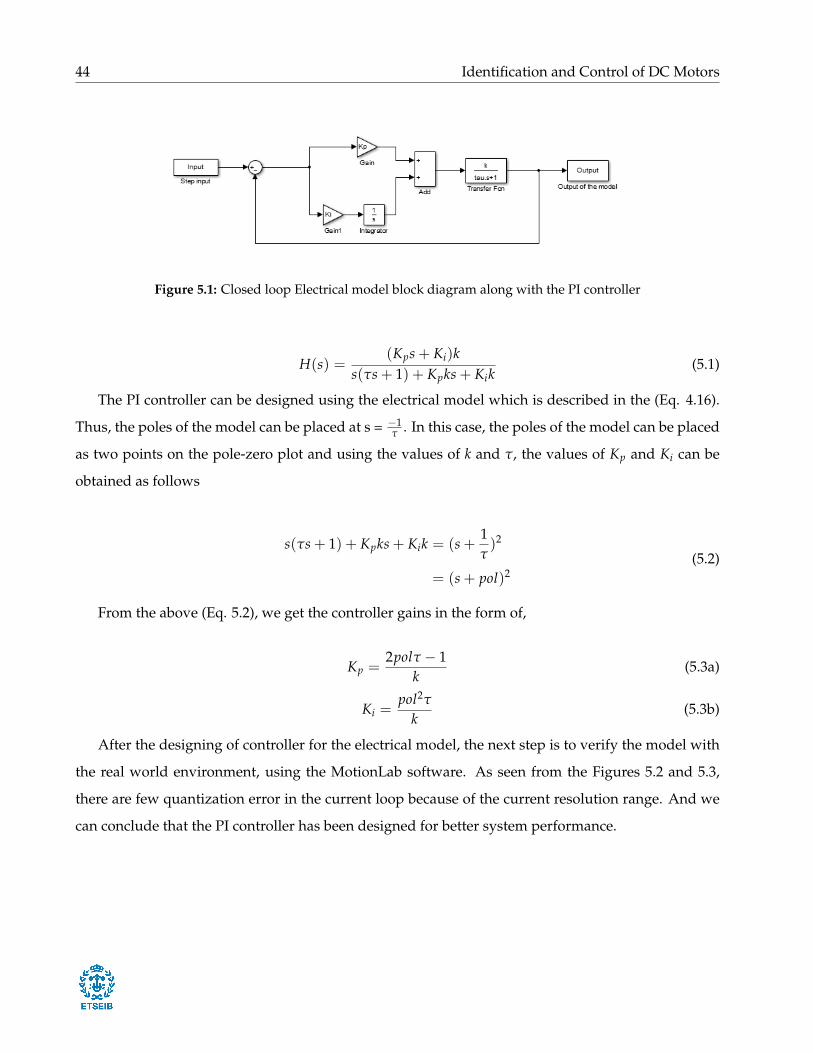
Figure 5.1: Closed loop Electrical model block diagram along with the PI controller
H(s) =(Kps + Ki)k
s(τs + 1) + Kpks + Kik(5.1)
The PI controller can be designed using the electrical model which is described in the (Eq. 4.16).
Thus, the poles of the model can be placed at s = −1τ . In this case, the poles of the model can be placed
as two points on the pole-zero plot and using the values of k and τ, the values of Kp and Ki can be
obtained as follows
s(τs + 1) + Kpks + Kik = (s +1τ)2
= (s + pol)2(5.2)
From the above (Eq. 5.2), we get the controller gains in the form of,
Kp =2polτ − 1
k(5.3a)
Ki =pol2τ
k(5.3b)
After the designing of controller for the electrical model, the next step is to verify the model with
the real world environment, using the MotionLab software. As seen from the Figures 5.2 and 5.3,
there are few quantization error in the current loop because of the current resolution range. And we
can conclude that the PI controller has been designed for better system performance.
Page 50
Identification and Control of DC Motors 45
MOT 37:
Figure 5.2: PI controller design verification of the model compared with real world
Kp = 38.9458; Ki = 6.8505e + 4;
Page 51
46 Identification and Control of DC Motors
MOT 53:
Figure 5.3: PI controller design verification of the model compared with real world
Kp = 15.3748; Ki = 2.6468e + 4;
Page 52
Identification and Control of DC Motors 47
5.2 Position loop
After the designing of the electrical model, the next step is determine the controller gains that are
again calculated using the pole placement technique. As described in the Section 2.3, the controller
design contains three unknown variables Kp, Ki and Kd which are defined as proportional gain, inte-
gral gain and derivative gain respectively.
As previously discussed, the PID controller can be calculated using poles of the closed loop model
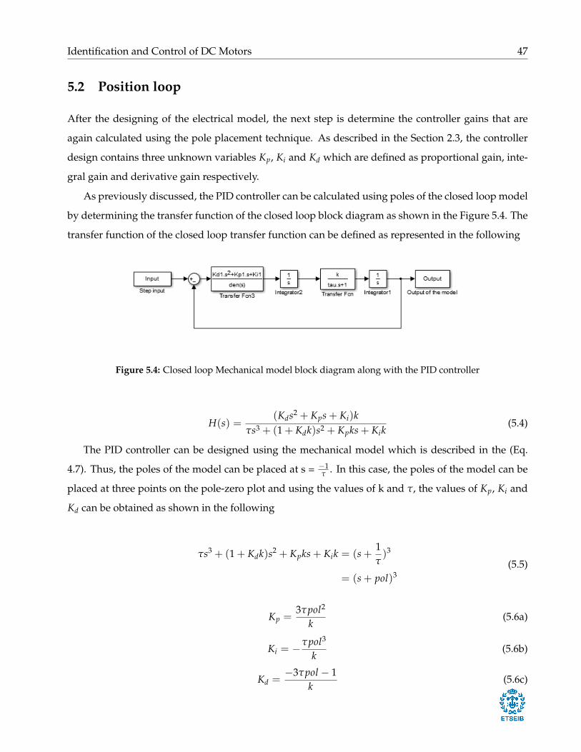
by determining the transfer function of the closed loop block diagram as shown in the Figure 5.4. The
transfer function of the closed loop transfer function can be defined as represented in the following
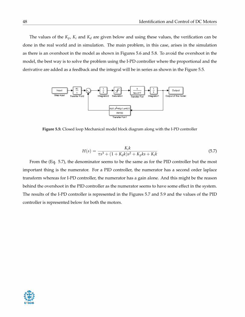
Figure 5.4: Closed loop Mechanical model block diagram along with the PID controller
H(s) =(Kds2 + Kps + Ki)k
τs3 + (1 + Kdk)s2 + Kpks + Kik(5.4)
The PID controller can be designed using the mechanical model which is described in the (Eq.
4.7). Thus, the poles of the model can be placed at s = −1τ . In this case, the poles of the model can be
placed at three points on the pole-zero plot and using the values of k and τ, the values of Kp, Ki and
Kd can be obtained as shown in the following
τs3 + (1 + Kdk)s2 + Kpks + Kik = (s +1τ)3
= (s + pol)3(5.5)
Kp =3τpol2
k(5.6a)
Ki = −τpol3
k(5.6b)
Kd =−3τpol − 1
k(5.6c)
Page 53
48 Identification and Control of DC Motors
The values of the Kp, Ki and Kd are given below and using these values, the verification can be
done in the real world and in simulation. The main problem, in this case, arises in the simulation
as there is an overshoot in the model as shown in Figures 5.6 and 5.8. To avoid the overshoot in the
model, the best way is to solve the problem using the I-PD controller where the proportional and the
derivative are added as a feedback and the integral will be in series as shown in the Figure 5.5.
Figure 5.5: Closed loop Mechanical model block diagram along with the I-PD controller
H(s) =Kik
τs3 + (1 + Kdk)s2 + Kpks + Kik(5.7)
From the (Eq. 5.7), the denominator seems to be the same as for the PID controller but the most
important thing is the numerator. For a PID controller, the numerator has a second order laplace
transform whereas for I-PD controller, the numerator has a gain alone. And this might be the reason
behind the overshoot in the PID controller as the numerator seems to have some effect in the system.
The results of the I-PD controller is represented in the Figures 5.7 and 5.9 and the values of the PID
controller is represented below for both the motors.
Page 54
Identification and Control of DC Motors 49
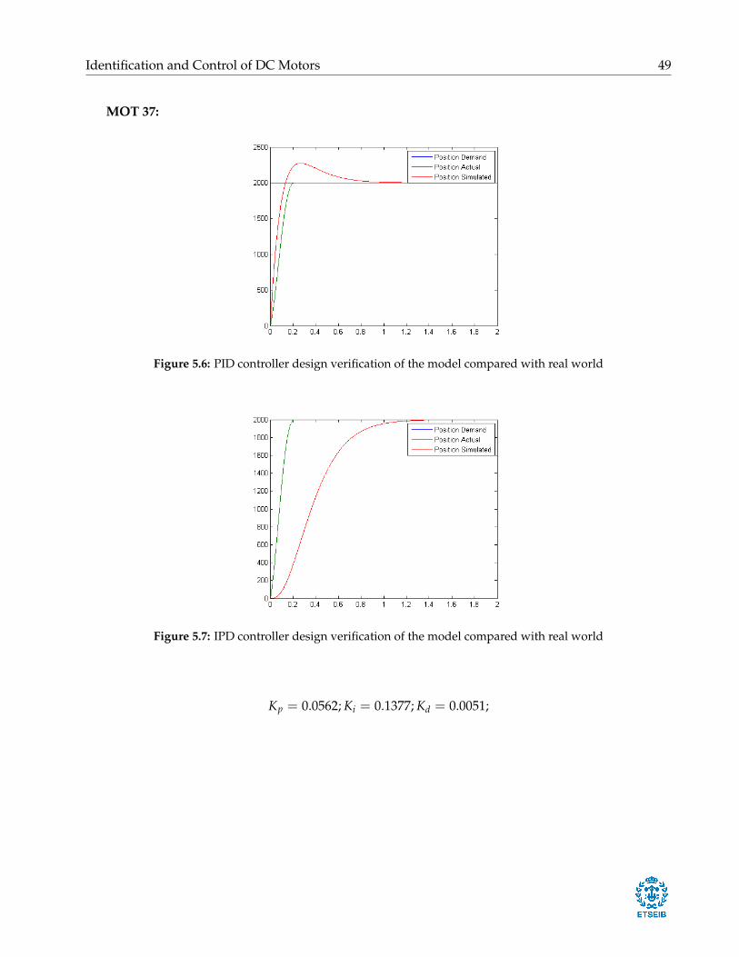
MOT 37:
Figure 5.6: PID controller design verification of the model compared with real world
Figure 5.7: IPD controller design verification of the model compared with real world
Kp = 0.0562; Ki = 0.1377; Kd = 0.0051;
Page 55
50 Identification and Control of DC Motors
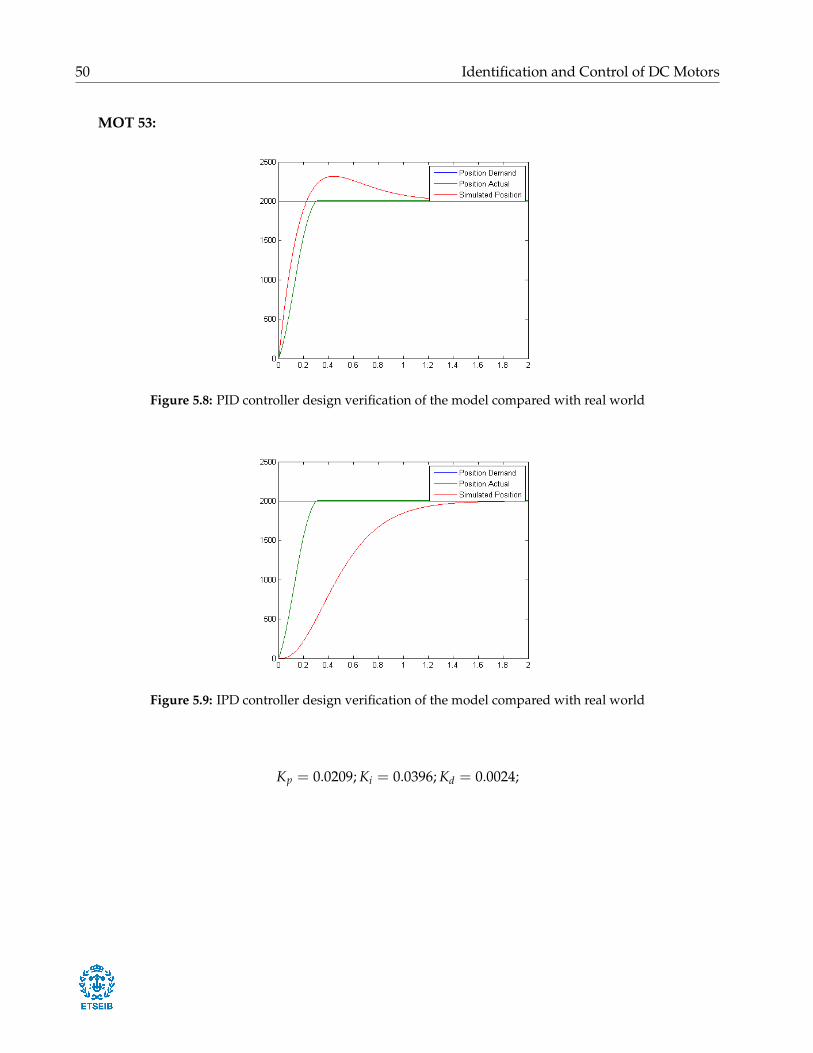
MOT 53:
Figure 5.8: PID controller design verification of the model compared with real world
Figure 5.9: IPD controller design verification of the model compared with real world
Kp = 0.0209; Ki = 0.0396; Kd = 0.0024;
Page 56
Identification and Control of DC Motors 51
Conclusions on the Control Design
First, to summarize, the controller has been designed in continuous time as the model identified
is in continuous time. Keeping in mind, however, that the current programs Ingenia version only
allows to implement PID controller. However, the suggestion is to develop different control schemes
to provide feasible results based on the results obtained above. The original presents continuous
PID controller with an overshoot, which corrects the I-PD controller continuum - slightly modified.
Another important conclusion, the designing of the controller was done using the pole placement
technique rather than using the bandwidth to design the controller as depicted in the Section 2.3.2.
Page 57
Chapter 6
Environment impact study
The application of the method presented in this paper for the identification and control of DC motors,
will have more impact on economic rather than environmental, but can perform some actions to min-
imize the effects of the project may cause to the environment. Developing codes for tuning controllers
provide constant driver directly based on the specification in the system bandwidth, reduces the cal-
culation time of the control problem. It is expected that the savings in time have a positive economic
impact.
The environmental impact of this project will be small as energy consumption mainly needed
to power the motor - is very low, and the life of your motor is sufficiently long as not to become
a problem. However, this impact can be reduced if the motors are recycled properly at the end of
its useful life: you can dismantle and classify expensive components in terms of materials, recover
the valuable materials that can still do service. It does not generate any toxic residue, smoke, etc.,
necessary to treat. That is why the environmental impact of the project will be minimal.
52
Page 58
Chapter 7
Conclusions
This chapter is not intended to repeat the analysis of the results of identification and control, which
has already made the final of each of the respective chapters. Instead, its goal is to give general
guidelines based on experience gained during the implementation of this project. Regarding the
identification of system, it is interesting to analyse the data estimation, especially the input of the
model. Clearly, the identification of the system depends on the input and the feedback of the encoder
as it is difficult to predict the proportional gain using the trial and error method. And also noticed is
the fact that the identification works better with continuous-time system than the discrete time.
Another interesting factor in this project is to eliminate the effect of integrators in the data pro-
vided that their presence known before: it has been verified that this substantially improves the re-
sults of the adjustment of the models. It is recalled that it was necessary to perform this procedure
for motor Ingenia because it had no speed sensor, and thus the appearance of a pure integrator gives
the measure of position output. With regard to control, it is interesting to note that the improvement
in motor response is obtained by passing the original PID structure alternatives I-PD because of the
overshoot.
In the near future, we will be concentrating on shaping the sensitivity function for the input of
the plant model. In this case, we will be shaping the sensitivity input function to control the peak
movement of the motor according to the saturation point. And also, we explore the frequency domain
techniques for design of the feedback model systems. Initially, it is based on identied continuous-
time systems of the motor involving the PID controller designed using the pole placement method
combined with sensitivity function in the frequency domain. In this case, the maximum peak has to
53
Page 59
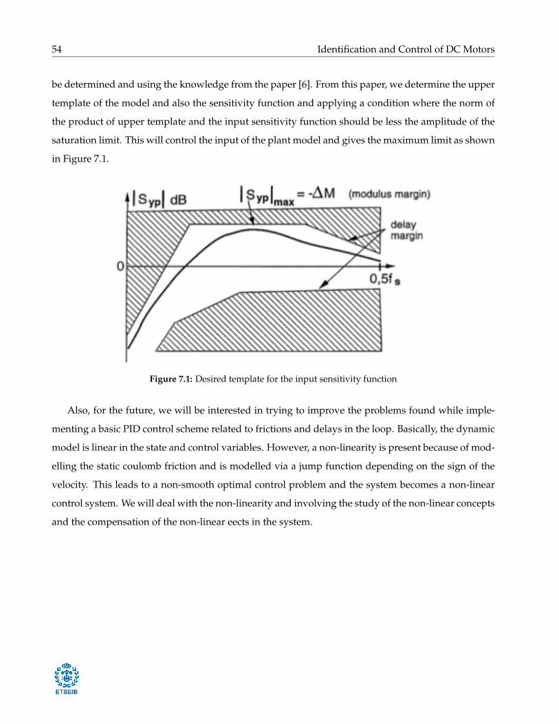
54 Identification and Control of DC Motors
be determined and using the knowledge from the paper [6]. From this paper, we determine the upper
template of the model and also the sensitivity function and applying a condition where the norm of
the product of upper template and the input sensitivity function should be less the amplitude of the
saturation limit. This will control the input of the plant model and gives the maximum limit as shown
in Figure 7.1.
Figure 7.1: Desired template for the input sensitivity function
Also, for the future, we will be interested in trying to improve the problems found while imple-
menting a basic PID control scheme related to frictions and delays in the loop. Basically, the dynamic
model is linear in the state and control variables. However, a non-linearity is present because of mod-
elling the static coulomb friction and is modelled via a jump function depending on the sign of the
velocity. This leads to a non-smooth optimal control problem and the system becomes a non-linear
control system. We will deal with the non-linearity and involving the study of the non-linear concepts
and the compensation of the non-linear eects in the system.
Page 60
Chapter 8
Cost of the project
In this chapter, the time invested, the assets used and various expenses will be discussed that have
been necessary for the development of this project.
The budget of this project is considered to be as follows:
Concept Cost [e]
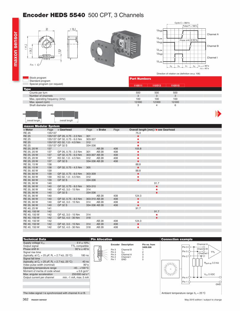
Maxon 253447 Motor Mot 37 290.00
Maxon 199809 Motor Mot 53 290.00
Pluto DC Servo drive 600.00
DC power supply (24V) 145.00
Software license Matlab R© 2000.00
Software license Simulink R© 3000.00
Assets cost 6325.00
Miscellaneous expenses 250.00
SubTotal 6575.00
Overhead costs (5%) 328.75
Salary 13750.00
Total cost 20,653.75
55
Page 61
56 Identification and Control of DC Motors
The table above gives the overall budget implementation of the project that was used for its de-
velopment. The first part of the table contains all the assets used in this whole project that have been
discussed in the Chapter 3.
Miscellaneous expenses includes, travel expenses, energy used, paper, food, etc., which is approx-
imately estimated during the project.
As for salary, it can be split into two parts, one for the project manager and the other for the
student. It is estimated that the project manager, who is assigned a salary of 50e / hour, has devoted
about 70 hours to the project, and in this case, two project managers were assigned, thus the salary
doubles; the student contemplates a salary of 15e / hour and 450 hours of total dedication to the
project.
Page 63
58 Identification and Control of DC Motors
Acknowledgements
I want to thank to my supervisor Vicenç Puig for guiding me and teaching me along this thesis.
And I also want to thank my advisors from the company Roger Juanpere and Rob Verhaart for helping
me provide their workspace for this thesis. I am very grateful for all your help and allow me to learn
so much.
A big thanks to my family, especially my mother for always supported me during all these years
and for allowing me to study these two years in Barcelona and undertake this journey and also shared
my pains and my joys during this run
And of course to all my roommates and friends, who helped me in motivating myself and helping
me throughout the semester.
Page 64
Chapter 9
Bibliography
[1] Mathworks. http://in.mathworks.com/help/ident/ug/what-is-a-process-model.html.
[2] Mathworks. http://in.mathworks.com/help/ident/ug/what-are-polynomial-models.html?
searchHighlight=polynomial%20model%20structure.
[3] Pablo Segovia Castillo. Vicenç Puig Cayuela. Identificació i control d’un motor de tipus voice coil.
2014.
[4] Karel J. Keesman. System identification techniques. In System Identification, volume 2.
[5] I. Landau and G. Zito. Digital control systems: Design, identication and implementation. 2006.
[6] I.D. LANDAU* and A. KARIMI. Robust digital control using pole placement with sensitivity
function shaping method. 1998.
[7] Lennart Ljung. Model structure selection and model validation. In System Identification: Theory for
the User, Second Edition, volume 16, pages 408–431. Linkoping University Sweden.
[8] Lennart Ljung. Practical issues of system identification, choice of signals. http://www.eolss.
net/EolssSampleChapters/C05/E6-43-12/E6-43-12-TXT-03.aspx.
[9] Luca Zaccarian. DC motors: dynamic model and control techniques, chapter 2.
59
Page 65
Appendix A
Matlab codes and Datasheet of Motors
1 c l e a r a l l
c l c
3
%\% E l e c t r i c a l I d e n t i f i c a t i o n Test ing
5 % Mutisine 2 0 : 2 0 : 4 0 0 0
f = f u l l f i l e ( ’ Torque ’ , ’ Output ’ , ’ Mult is ine20 . csv ’ ) ;
7 load ( f ) ;
t = Mult is ine20 ( : , 1 ) ; t = t /10000;
9 T_actual = Mult is ine20 ( : , 2 ) ;
T_demand = Mult is ine20 ( : , 3 ) ;
11
Ts = 1/10000;
13
% Transfer funct ion i d e n t i f i e d model
15
load ( ’P1_M50 . mat ’ ) ;
17
% Gz = t f ( oe111 . B , oe111 . F , Ts ) ;
19 G = t f ( P1 ) ; % d2c (Gz) ;
[num, den ] = t f d a t a (G, ’v ’ ) ;
21 Gz = c2d (G, Ts ) ;
23 k = num( 2 ) ; tau = den ( 1 ) ;
R = 1/k
25 L = tau∗R
60
Page 66
Identification and Control of DC Motors 61
27 %% PI c o n t r o l l e r design
syms Kp1 Ki1 s ;
29 p = pole (G) ;
C1 = ( s ^2) +((1+Kp1∗k ) /tau ) ∗ s +(k∗Ki1/tau ) ;
31 C2 = ( s + p ) ^2;
33 S = c o e f f s ( C1−C2 , s ) ;
35 Kp1 = −double ( so lve ( S ( 2 ) ,Kp1 ) )
Ki1 = double ( so lve ( S ( 1 ) , Ki1 ) )
37 % Ki1 = (1/ a ) ∗ (2 ∗p−d−b∗Kp1 ) ;
% Kp1 = (1/b ) ∗ (2 ∗p−d−a∗Ki1 ) ;
39
Kp = Kp1∗ (2^15) /(2^6)
41 Ki = Ki1∗ (2^15) ∗Ts /(2^6)
43 C = t f ( [ Kp1 Ki1 ] , [ 1 0 ] ) ;
45 sys = feedback (C∗G, 1 ) ;
Listing A.1: Identification and control of Current loop
1 c l e a r a l l ;
c l c
3
%% Mechanical i d e n t i f i c a t i o n with v e l o c i t y output
5 f = f u l l f i l e ( ’ P o s i t i o n ’ , ’ Output ’ , ’ Mult is ine4000 ’ , ’ Mult is ine2000_1 . csv ’ ) ;
load ( f ) ;
7 t = Mult is ine2000_1 ( : , 1 ) ; t = t /1000; tmax = max( t ) ;
P_actual = Mult is ine2000_1 ( : , 2 ) ;
9 P_demand = Mult is ine2000_1 ( : , 3 ) ;
11 Ts = 1/1000;
13 y = zeros ( length ( P_actual ) , 1 ) ;
15 y ( 1 ) = P_actual ( 1 ) ;
k = 2 ;
Page 67
62 Identification and Control of DC Motors
17
while ( k<501)
19 y ( k ) = ( P_actual ( k )−P_actual ( k−1) ) /(1∗Ts ) ; %dona y ( k ) ∗Ts degut a l ’ aproximacio
k = k +1;
21 end
23 %% Transfer funct ion deduction
25 f = f u l l f i l e ( ’ P o s i t i o n ’ , ’ Output ’ , ’ Mult is ine4000 ’ , ’ P2000 . mat ’ ) ;
load ( f ) ;
27
Gmotor = t f ( P1 ) ;
29 [num, den ] = t f d a t a ( P1 , ’v ’ ) ;
k = num( 2 ) ; tau = den ( 1 ) ;
Listing A.2: Identification of Position Loop
1 c l e a r a l l ;
c l c
3
%% Mechanical i d e n t i f i c a t i o n with v e l o c i t y output
5 f = f u l l f i l e ( ’ P o s i t i o n ’ , ’ Output ’ , ’ Mult is ine4000 ’ , ’ Mult is ine2000_3 . csv ’ ) ;
load ( f ) ;
7 t = Mult is ine2000_3 ( : , 1 ) ; t = t /1000;
P_actual = Mult is ine2000_3 ( : , 2 ) ;
9 P_demand = Mult is ine2000_3 ( : , 3 ) ;
11 Ts = 1/1000;
13 y = zeros ( length ( P_actual ) , 1 ) ;
15 y ( 1 ) = P_actual ( 1 ) ;
k = 3 ;
17
while ( k<501)
19 y ( k ) = ( P_actual ( k )−P_actual ( k−1) ) /(1∗Ts ) ;
k = k +1;
21 end
Page 68
Identification and Control of DC Motors 63
23 %% Transfer funct ion deduction
25 f = f u l l f i l e ( ’ P o s i t i o n ’ , ’ Output ’ , ’ Mult is ine4000 ’ , ’ P2000 . mat ’ ) ;
load ( f ) ;
27
Gmotor = t f ( P1 ) ;
29 [num, den ] = t f d a t a ( P1 , ’v ’ ) ;
31 %% Bode
f1 = 0 : 0 . 0 1 : 1 0 0 ;
33 f2 = 1 0 1 : 1 : 4 0 0 ;
f r = [ f1 f2 ] ;
35 wr = 2∗pi∗ f r ;
Fs = 1000 ;
37 Ts = 1/Fs ;
39 [ gu , fu ] = t d f ( P_demand , f r , Ts , 0 ) ;
[ ga , fa ] = t d f ( P_actual , f r , Ts , 0 ) ;
41 [ gy , fy ] = t d f ( y , f r , Ts , 0 ) ;
43
f i g u r e ( 1 )
45 t i t l e ( ’ Frequency Response of Motor ’ ) ;
bodemag ( Gmotor , ’ g ’ )
47 grid on
hold on
49 % bodemag ( Gmotor , ’ b ’ )
% bodemag ( Cmotor , ’ b ’ )
51 % bodemag ( sysMotor , ’m’ )
semilogx ( wr , 20∗ log10 ( gy ./ gu ) , ’ r∗ ’ , ’ MarkerSize ’ , 3 )
53 xlim ([−0.1 1 0 0 0 0 0 ] ) ; ylim ([−20 6 0 ] ) ;
% f i l e _ p i c = f u l l f i l e ( ’ Pics ’ , ’ Mult is ine1000 ’ , ’ P4000 ’ , ’ Mult is ine4000_3 . png ’ ) ;
55 % saveas ( gcf , f i l e _ p i c ) ;
Listing A.3: Data estimation of Position Loop
Page 69
64 Identification and Control of DC Motors
2 c l e a r a l l ;
c l c
4
%% Mechanical i d e n t i f i c a t i o n 5% amplitude noise on step
6 f = f u l l f i l e ( ’ P o s i t i o n ’ , ’ Output ’ , ’ SamplePID2 . csv ’ ) ;
load ( f ) ;
8 t = SamplePID2 ( : , 1 ) ; t = t /1000; tmax = max( t ) ;
P_actual = SamplePID2 ( : , 2 ) ;
10 P_demand = SamplePID2 ( : , 3 ) ;
12 Ts = 1/1000;
14 y = zeros ( length ( P_actual ) , 1 ) ;
16 y ( 1 ) = P_actual ( 1 ) ;
k = 2 ;
18
while ( k<501)
20 y ( k ) = ( P_actual ( k )−P_actual ( k−1) ) /(1∗Ts ) ; %dona y ( k ) ∗Ts degut a l ’ aproximacio
k = k +1;
22 end
24 %% Transfer funct ion deduction
26 f = f u l l f i l e ( ’ P o s i t i o n ’ , ’ Output ’ , ’ Mult is ine4000 ’ , ’ P2000 . mat ’ ) ;
load ( f ) ;
28
Gmotor = t f ( P1 ) ;
30 [num, den ] = t f d a t a ( P1 , ’v ’ ) ;
k = num( 2 ) ; tau = den ( 1 ) ;
32
%% C o n t r o l l e r design
34 pol = −pole ( Gmotor ) ; Ks = 65536 ;
Kd1 = (3 ∗pol∗ tau−1)/k ;
36 Kp1 = (3 ∗ ( pol ^2)∗ tau ) /k ;
Ki1 = ( ( ( pol ) ^3)∗ tau ) /k ;
38
Page 70
Identification and Control of DC Motors 65
Kp = Kp1∗Ks
40 Ki = Ki1∗ ( Ks∗Ts )
Kd = Kd1∗ ( Ks/Ts )
42
y1 = [ t y ] ;
44 Demand_in = [ t P_demand ] ;
Actual = [ t P_actual ] ;
46 sim ( ’ V e r i f i c a t i o n ’ ) ;
48 f i g u r e
p l o t (Demand . time , Demand . Data , Real . time , Real . Data , P o s i t i o n . time , P o s i t i o n . Data ) ;
50 legend ( ’ P o s i t i o n Demand ’ , ’ P o s i t i o n Actual ’ , ’ P o s i t i o n Simulated ’ ) ;
52 f i g u r e
p l o t (Demand . time , Demand . Data , Real . time , Real . Data , PositionMotionLab . time , PositionMotionLab .
Data ) ;
54 legend ( ’ P o s i t i o n Demand ’ , ’ P o s i t i o n Actual ’ , ’ P o s i t i o n Simulated ’ ) ;
% f i l e _ p i c = f u l l f i l e ( ’ Pics ’ , ’ SamplePID . png ’ ) ;
56 % saveas ( gcf , f i l e _ p i c ) ;
58 % f i g u r e
% p l o t ( y . time , y . Data , V e l o c i t y . time , V e l o c i t y . Data ) ;
60 % legend ( ’ V e l o c i t y actual ’ , ’ V e l o c i t y simulated ’ ) ;
Listing A.4: Control of Position Loop
Page 71
170
max
on
-m
ax
6 9 12 18 24 30 36 485870 4940 4680 5280 5930 5870 5830 3870154 83.5 58.6 44.9 38.7 30.6 25.3 11.84110 3090 2920 3590 4210 4160 4100 209036.5 35 37.2 38.3 37.3 37.5 37.1 373.95 2.12 1.6 1.23 1.01 0.806 0.66 0.328127 95.3 101 122 130 130 127 81.613.2 5.58 4.19 3.78 3.42 2.7 2.17 0.778 76 77 79 80 80 80 76
0.454 1.61 2.86 4.76 7.03 11.1 16.6 68.60.066 0.209 0.416 0.739 1.04 1.66 2.43 9.719.58 17.1 24.1 32.2 38.2 48.2 58.3 117996 559 396 297 250 198 164 81.947.2 52.8 47 44 46 45.6 46.6 48.221.9 21.7 21.4 21.3 21.3 21.3 21.4 21.544.2 39.2 43.5 46.2 44.2 44.6 43.8 42.6
M 1:2
236651 236652 236653 236654 236655 236656 236657 236658353220 353221 353222 353223 353224 353225 353226 353227
7.5 K/W 2.1 K/W 17.8 s 791 s -20…+85°C +125°C
0.12 - 0.22 mm 0.025 mm 7.6 N 110 N
2000 N 32 N
0.12 - 0.22 mm 0.012 mm 5.0 N 110 N
2000 N 10.5 N
1 13 210 g
ESCON Module 24/2 378ESCON 36/2 DC 378ESCON Module 50/5 379ESCON 50/5 380EPOS2 24/2 386EPOS2 Module 36/2 386EPOS2 24/5, EPOS2 50/5 387EPOS2 P 24/5 390EPOS3 70/10 EtherCAT 393MAXPOS 50/5 396
Stock programStandard programSpecial program (on request)
Specifi cations Operating Range Comments
n [rpm] Continuous operationIn observation of above listed thermal resistance (lines 17 and 18) the maximum permissible winding temperature will be reached during continuous op-eration at 25°C ambient.= Thermal limit.
Short term operationThe motor may be briefl y overloaded (recurring).
Assigned power rating
maxon Modular System Overview on page 20–25
Part Numbers
maxon DC motor May 2015 edition / subject to change
-max 32 ∅32 mm, Graphite Brushes, 15 Watt
Values at nominal voltage1 Nominal voltage V2 No load speed rpm3 No load current mA4 Nominal speed rpm5 Nominal torque (max. continuous torque) mNm6 Nominal current (max. continuous current) A7 Stall torque mNm8 Stall current A9 Max. effi ciency %
Characteristics10 Terminal resistance Ω11 Terminal inductance mH12 Torque constant mNm/A13 Speed constant rpm/V14 Speed / torque gradient rpm/mNm15 Mechanical time constant ms16 Rotor inertia gcm2
Motor Data
Thermal data17 Thermal resistance housing-ambient 18 Thermal resistance winding-housing 19 Thermal time constant winding 20 Thermal time constant motor 21 Ambient temperature 22 Max. winding temperature
Mechanical data (ball bearings)23 Max. speed 6000 rpm24 Axial play 25 Radial play 26 Max. axial load (dynamic) 27 Max. force for press fi ts (static)
(static, shaft supported) 28 Max. radial load, 5 mm from fl ange
Mechanical data (sleeve bearings)23 Max. speed 6000 rpm24 Axial play 25 Radial play 26 Max. axial load (dynamic) 27 Max. force for press fi ts (static)
(static, shaft supported) 28 Max. radial load, 5 mm from fl ange
Other specifi cations29 Number of pole pairs 30 Number of commutator segments 31 Weight of motor Values listed in the table are nominal. Explanation of the fi gures on page 107.
Option Sleeve bearings in place of ball bearings
Planetary Gearhead∅32 mm0.75 - 6.0 NmPage 303–308Spur Gearhead∅38 mm0.1 - 0.6 NmPage 313
Encoder HED_ 5540500 CPT, 3 channelsPage 363/365
with terminalswith cables
Recommended Electronics:Notes Page 22
Encoder MR256 - 1024 CPT,3 channelsPage 356
Spindle Drive∅32 mmPage 334–336
1506_DC_motor.indd 170 07.05.15 09:22
Page 72
max
on
sen
sor
362
RE 25 135/137 75.3RE 25 135/137 GP 26, 0.75 - 2.0 Nm 301 •RE 25 135/137 GP 32, 0.75 - 6.0 Nm 303-307 •RE 25 135/137 KD 32, 1.0 - 4.5 Nm 312 •RE 25 135/137 GP 32 S 334-336 •RE 25, 20 W 137 AB 28 408 105.8RE 25, 20 W 137 GP 26, 0.75 - 2.0 Nm 301 AB 28 408 •RE 25, 20 W 137 GP 32, 0.75 - 6.0 Nm 303-307 AB 28 408 •RE 25, 20 W 137 KD 32, 1.0 - 4.5 Nm 312 AB 28 408 •RE 25, 20 W 137 GP 32 S 334-336 AB 28 408 •RE 30, 15 W 138 88.8RE 30, 15 W 138 GP 32, 0.75 - 4.5 Nm 305 •RE 30, 60 W 139 88.8RE 30, 60 W 139 GP 32, 0.75 - 6.0 Nm 303-309 •RE 30, 60 W 139 KD 32, 1.0 - 4.5 Nm 312 •RE 30, 60 W 139 GP 32 S 334-336 •RE 35, 90 W 140 91.7RE 35, 90 W 140 GP 32, 0.75 - 8.0 Nm 303-310 •RE 35, 90 W 140 GP 42, 3.0 - 15 Nm 314 •RE 35, 90 W 140 GP 32 S 334-336 •RE 35, 90 W 140 AB 28 408 124.3RE 35, 90 W 140 GP 32, 0.75 - 8.0 Nm 303-310 AB 28 408 •RE 35, 90 W 140 GP 42, 3.0 - 15 Nm 314 AB 28 408 •RE 35, 90 W 140 GP 32 S 334-336 AB 28 408 •RE 40, 25 W 141 91.7RE 40, 150 W 142 91.7RE 40, 150 W 142 GP 42, 3.0 - 15 Nm 314 •RE 40, 150 W 142 GP 52, 4.0 - 30 Nm 318 •RE 40, 150 W 142 AB 28 408 124.3RE 40, 150 W 142 GP 42, 3.0 - 15 Nm 314 AB 28 408 •RE 40, 150 W 142 GP 52, 4.0 - 30 Nm 318 AB 28 408 •
110511 110513 110515
500 500 5003 3 3
100 100 100 12 000 12 000 12 000
3 4 6
maxon sensor May 2015 edition / subject to change
Stock programStandard programSpecial program (on request)
Encoder HEDS 5540 500 CPT, 3 Channels
maxon Modular System+ Motor Page + Gearhead Page + Brake Page Overall length [mm] / • see Gearhead
Part Numbers
TypeCounts per turnNumber of channelsMax. operating frequency (kHz)Max. speed (rpm)Shaft diameter (mm)
Direction of rotation cw (definition cw p. 106)
Technical Data Pin Allocation Connection exampleSupply voltage VCC 5 V ± 10%Output signal TTL compatiblePhase shift Φ 90°e ± 45°eSignal rise time (typically, at CL = 25 pF, RL = 2.7 kW, 25 °C) 180 nsSignal fall time (typically, at CL = 25 pF, RL = 2.7 kW, 25 °C) 40 nsIndex pulse width (nominal) 90°eOperating temperature range -40…+100 °CMoment of inertia of code wheel ≤ 0.6 gcm2
Max. angular acceleration 250 000 rad s-2
Output current per channel min. -1 mA, max. 5 mA
The index signal I is synchronized with channel A or B. Ambient temperature range JU = 25 °C
Encoder Description Pin no. from 3409.506Pin 5 Channel B 1Pin 4 VCC 2Pin 3 Channel A 3Pin 2 Channel I 4Pin 1 GND 5
Channel A
Channel B
Channel I
VCC 5 VDC
Rpull-up 3.3 k
GND
TTL
Pin 3
Pin 5
Pin 2
Pin 4
Pin 1
s∆ 45°e<s2 s = 90°e1..4s1s4s3
U
U
U
U
U
U
High
High
High
Low
Low
Low
90°e
Channel A
Channel B
Channel I
Cycle C = 360°e
Pulse P = 180°e
Phase shift
overall length overall length
Page 73
max
on
sen
sor
363
RE 25, 20 W 136 63.8RE 25, 20 W 136 GP 26, 0.75 - 2.0 Nm 301 •RE 25, 20 W 136 GP 32, 0.75 - 4.5 Nm 303 •RE 25, 20 W 136 GP 32, 0.75 - 6.0 Nm 304/307 •RE 25, 20 W 136 KD 32, 1.0 - 4.5 Nm 312 •RE 25, 20 W 136 GP 32 S 334-336 •RE 25, 20 W 136 AB 28 408 94.3RE 25, 20 W 136 GP 22, 0.5 Nm 293 •RE 25, 20 W 136 GP 26, 0.75 - 2.0 Nm 301 AB 28 408 •RE 25, 20 W 136 GP 32, 0.75 - 4.5 Nm 303 AB 28 408 •RE 25, 20 W 136 GP 32, 0.75 - 6.0 Nm 304/307 AB 28 408 •RE 25, 20 W 136 KD 32, 1.0 - 4.5 Nm 312 AB 28 408 •RE 25, 20 W 136 GP 32 S 334-336 AB 28 408 •RE 50, 200 W 143 128.7RE 50, 200 W 143 GP 52, 4 - 30 Nm 319 •RE 50, 200 W 143 GP 62, 8 - 50 Nm 320 •RE 65, 250 W 144 157.3RE 65, 250 W 144 GP 81, 20 - 120 Nm 321 •A-max 26 162-168 63.1A-max 26 162-168 GP 26, 0.75 - 4.5 Nm 301 •A-max 26 162-168 GS 30, 0.07 - 0.2 Nm 302 •A-max 26 162-168 GP 32, 0.75 - 4.5 Nm 303 •A-max 26 162-168 GP 32, 0.75 - 6.0 Nm 304/308 •A-max 26 162-168 GS 38, 0.1 - 0.6 Nm 313 •A-max 26 162-168 GP 32 S 334-336 •A-max 32 170/172 82.3A-max 32 170/172 GP 32, 0.75 - 6.0 Nm 303-308 •A-max 32 170/172 GS 38, 0.1 - 0.6 Nm 313 •A-max 32 170/172 GP 32 S 334-336 •EC 32, 80 W 214 78.4EC 32, 80 W 214 GP 32, 0.75 - 6.0 Nm 303-309 •EC 32, 80 W 214 GP 32 S 334-336 •EC 40, 170 W 215 103.4EC 40, 170 W 215 GP 42, 3.0 - 15 Nm 314 •EC 40, 170 W 215 GP 52, 4.0 - 30 Nm 318 •
110511 110513 110515 110517
500 500 500 5003 3 3 3
100 100 100 10012 000 12 000 12 000 12 000
3 4 6 8
May 2015 edition / subject to change maxon sensor
Stock programStandard programSpecial program (on request)
Encoder HEDS 5540 500 CPT, 3 Channels
maxon Modular System+ Motor Page + Gearhead Page + Brake Page Overall length [mm] / • see Gearhead
Part Numbers
TypeCounts per turnNumber of channelsMax. operating frequency (kHz)Max. speed (rpm)Shaft diameter (mm)
Direction of rotation cw (definition cw p. 106)
Technical Data Pin Allocation Connection exampleSupply voltage VCC 5 V ± 10%Output signal TTL compatiblePhase shift Φ 90°e ± 45°eSignal rise time (typically, at CL = 25 pF, RL = 2.7 kW, 25 °C) 180 nsSignal fall time (typically, at CL = 25 pF, RL = 2.7 kW, 25 °C) 40 nsIndex pulse width 90°eOperating temperature range -40…+100 °CMoment of inertia of code wheel ≤ 0.6 gcm2
Max. angular acceleration 250 000 rad s-2
Output current per channel min. -1 mA, max. 5 mA
The index signal I is synchronized with channel A or B. Ambient temperature range JU = 25 °C
Encoder Description Pin no. from 3409.506Pin 5 Channel B 1Pin 4 VCC 2Pin 3 Channel A 3Pin 2 Channel I 4Pin 1 GND 5
Channel A
Channel B
Channel I
VCC 5 VDC
Rpull-up 3.3 k
GND
TTL
Pin 3
Pin 5
Pin 2
Pin 4
Pin 1
s∆ 45°e<s2 s = 90°e1..4s1s4s3
U
U
U
U
U
U
High
High
High
Low
Low
Low
90°e
Channel A
Channel B
Channel I
Cycle C = 360°e
Pulse P = 180°e
Phase shift
Page 74
Rango de funcionamiento Leyenda Detalles en página 49
Rango recomendado de funcionamiento
Funcionamiento continuoTeniendo en cuenta los valores de resistencia térmi-ca antes mencionados (líneas 19 y 20). El rotor al-canzará la máxima temperatura durante funciona-miento continuo a 25°C de temperatura ambiente =límite térmico.
Funcionamiento intermitenteEl motor puede ser sobrecargado durante cortos pe-ríodos (cíclicamente).
Motor con bobinado de alta resistencia
Motor con bobinado de baja resistencia
n [rpm]
max
onD
Cm
otor
Especificaciones
Programa StockPrograma EstándarPrograma Especial (¡previo encargo!)
Números de Referencia
Edición de Agosto de 2004 / Sujeto a modificaciones maxon DC motor 81
Sistema Modular maxon Esquema general en página 17 - 21
118804
118797
RE 36 36 mm, Escobillas de grafito, 70 Vatios
Juego axial 0.05 - 0.15 mm Carga máx. en el rodamiento a bolas
axial (dinámica)sin pretensado 5.6 Npretensado 2.4 N
radial (a 5 mm de la brida) 28 NFuerza de empuje a presión (estática) 110 N(idem, con eje sostenido) 1200 N
Juego radial en rodamiento a bolas 0.025 mm Temperatura ambiente -20 ... +100°C Máx. temperatura del rotor +125°C Número de delgas del colector 13 Peso del motor 350 g Imàn permanente de 2 polos Los datos de la tabla son valores nominales.
Para las tolerancias aplicables (ver página 43) ypara detalles adicionales solicite nuestro serviciode asistencia por ordenador.
Para este motor, las tolerancias pueden variar dela especificación estándar.
100 200 300
9000
7000
5000
3000
1000
70 Watt
0.5 1.0 1.5 2.0 2.5 3.0
2 4 6 8 10 12
M [mNm]I [A]
I [A]
Reductor Planetario32 mm0.75 - 4.5 NmDetalles página 213
Reductor Planetario32 mm0.4 - 2.0 NmDetalles página 216Reductor Planetario42 mm3 - 15 NmDetalles página 218
Tacodinamos CC22 mm0.52 VDetalles página 246
Encoder DigitalHP HEDS 5540500 ppv, 3 canalesDetalles pág. 236Encoder DigitalHP HEDL 5540500 ppv, 3 canalesDetalles página 238
118797 118798 118799 118800 118801 118802 118803 118804 118805 118806 118807 118808 118809 118810Datos del motor
1 Potencia nominal asignada W 70 70 70 70 70 70 70 70 70 70 70 70 70 702 Tensión nominal Volt 18.0 24.0 32.0 42.0 42.0 48.0 48.0 48.0 48.0 48.0 48.0 48.0 48.0 48.03 Velocidad en vacío rpm 6610 6210 6790 7020 6340 6420 5220 4320 3450 2830 2280 1780 1420 11804 Par de arranque mNm 730 783 832 865 786 785 627 504 403 326 258 198 158 1275 Relación velocidad / par rpm / mNm 9.23 8.05 8.27 8.19 8.14 8.25 8.41 8.65 8.67 8.80 8.96 9.17 9.21 9.516 Corriente en vacío mA 153 105 89 70 61 55 42 33 25 20 15 12 9 77 Corriente de arranque A 28.6 21.5 18.7 15.3 12.6 11.1 7.22 4.80 3.06 2.04 1.30 0.784 0.501 0.3348 Resistencia en bornes Ohm 0.628 1.11 1.71 2.75 3.35 4.32 6.65 10.00 15.7 23.5 36.8 61.3 95.8 1449 Máx. velocidad permitida rpm 8200 8200 8200 8200 8200 8200 8200 8200 8200 8200 8200 8200 8200 8200
10 Máx. corriente en continuo A 3.18 2.44 1.99 1.59 1.44 1.27 1.03 0.847 0.679 0.556 0.445 0.346 0.277 0.22611 Máx. par permanente mNm 81 88.8 88.5 89.8 90.4 90.1 89.8 89.0 89.2 88.8 88.1 87.3 87.2 85.812 Máx. potencia útil a tensión nominal W 123 125 146 157 129 131 84.9 56.4 36.0 23.9 15.2 9.09 5.78 3.8213 Máx. rendimiento % 84 85 86 86 86 86 85 84 82 81 79 77 75 7214 Constante de par mNm / A 25.5 36.4 44.5 56.6 62.6 70.7 86.9 105 131 160 198 253 315 38015 Constante de velocidad rpm / V 375 263 215 169 152 135 110 90.9 72.7 59.8 48.2 37.8 30.3 25.116 Constante de tiempo mecánica ms 6 6 6 6 6 6 6 6 6 6 6 6 6 617 Inercia del rotor gcm2 60.2 67.7 65.2 65.4 65.6 64.6 63.3 61.5 61.3 60.3 59.2 57.8 57.5 55.718 Inductancia en bornes mH 0.10 0.20 0.30 0.49 0.60 0.76 1.15 1.68 2.62 3.87 5.96 9.70 15.10 21.9019 Resistencia térmica carcasa / ambiente K / W 6.4 6.4 6.4 6.4 6.4 6.4 6.4 6.4 6.4 6.4 6.4 6.4 6.4 6.420 Resistencia térmica rotor / carcasa K / W 3.4 3.4 3.4 3.4 3.4 3.4 3.4 3.4 3.4 3.4 3.4 3.4 3.4 3.421 Constante de tiempo térmica de bobinado s 38 43 41 41 41 41 40 39 39 38 37 36 36 35
Reductor Planetario32 mm1.0 - 6.0 NmDetalles página 214
Encoder Digital MR256 - 1024 ppv,3 canalesDetalles página 233
M 1:2
Electrónicas Recomendadas:ADS 50/5 página 253ADS 50/10 253ADS_E 50/5, 50/10 254EPOS 24/5 263MIP 50 265Notas 17
Page 75
Edición de agosto de 2010 / Sujeto a modificaciones maxon sensor 269
Programa StockPrograma EstándarPrograma Especial (previo encargo)
max
onse
nsor
Longitud total Longitud total
Datos técnicos RE 75 Ejemplo de conexiónTensión de alimentación 5 V 10 %
Tipo ensanchado del conectorTipo SOURIAU 8GM-QL2-12P1 VCC2 N.C. (no conectar)3 GND4 N.C. (no conectar)5 Canal I (Index)6 Canal I7 Canal B8 Canal B9 Canal A10 Canal A11 N.C. (no conectar)12 N.C. (no conectar)Conectores recomendadosTipo SOURIAU 8GM-DM2-12S(metal, salida recta:maxon N° de artículo 2675.538) o8G-V2-12S (plástico, ángulo 90°:maxon N° de artículo 2675.539)
Resistencia en bornes R = típica 120
Señal de salida EIA Standard RS 422Drivers integrados: DS26LS31Desfase 90°e ± 45°eTiempo del frente de subida(típico con CL = 25 pF, RL = 2.7 k, 25°C) 180 nsTiempo del frente de bajada(típico con CL = 25 pF, RL = 2.7 k, 25°C) 40 nsAnchura de pulso index 90°eRango de temperaturas -40 ... +100°CMomento de la inercia de la rueda de código 0.6 gcm2
Máx. aceleración angular 250 000 rad s-2
Corriente de salida por canal min. -20 mA, max. 20 mAOption 1000 ppv, 2 canales
La señal del canal index I es sincronizada con el canalA y con el B.
Encoder 500 ppv, 3 canales, con line driver RS
Sistema Modular maxon+ Motor Página + Reductor Página + Freno Página Longitud total [mm] / ver reductorRE 50, 150 W 83 128.7RE 50, 150 W 83 GP 52, 4 - 30 Nm 242
RE 50, 150 W 83 GP 62, 8 - 50 Nm 243
RE 65, 250 W 84 157.3RE 65, 250 W 84 GP 81, 20 - 120 Nm 244
EC 32, 80 W* 153 78.4EC 32, 80 W* 153 GP 32, 0.75 - 4.5 Nm 230
EC 32, 80 W* 153 GP 32, 0.75 - 6.0 Nm 232/234
EC 32, 80 W* 153 GP 32 S 249-251
EC 40, 120 W* 154 88.4EC 40, 120 W* 154 GP 42, 3.0 - 15 Nm 238
EC 40, 120 W* 154 GP 52, 4.0 - 30 Nm 241
EC-max 30, 40 W 166 62.6EC-max 30, 40 W 166 GP 32, 1 - 6 Nm 234
EC-max 30, 40 W 166 AB 20 316 101.7EC-max 30, 40 W 166 GP 32, 1 - 6 Nm 234 AB 20 316
EC-max 30, 40 W 166 GP 32 S
EC-max 30, 40 W 166 GP 32, 4.0 - 8.0 Nm 235EC-max 30, 60 W 167 84.6EC-max 30, 60 W 167 GP 32, 4.0 - 8.0 Nm 235EC-max 30, 60 W 167 GP 42, 3 - 15 Nm 239
EC-max 30, 60 W 167 AB 20 316 123.7EC-max 30, 60 W 167 GP 42, 3 - 15 Nm 239 AB 20 316
EC-max 40, 70 W 168 81.4EC-max 40, 70 W 168 GP 42, 3 - 15 Nm 239
EC-max 40, 70 W 168 AB 28 317 121.4EC-max 40, 70 W 168 GP 42, 3 - 15 Nm 239 AB 28 317
EC-max 40, 120 W 169 111.4EC-max 40, 120 W 169 GP 52, 4 - 30 Nm 242
EC-max 40, 120 W 169 AB 28 317 151.4EC-max 40, 120 W 169 GP 52, 4 - 30 Nm 242 AB 28 317
* Conexión siehe Página 268
Números de Referencia
110512 110514 110516 110518Tipo
Número de pulsos por vuelta 500 500 500 500Número de canales 3 3 3 3Máx. frecuencia de funcionamiento (kHz) 100 100 100 100Máx. velocidad (rpm) 12000 12000 12000 12000Diámetro de eje (mm) 3 4 6 8
Sentido de rotación cw (Definitión cw P. 48)
R
R
R
Terminación electrónica delusuario. CI recomendados- MC 3486- SN 75175- AM 26 LS 32
Canal A
Canal A
Canal B
Canal B
Canal I
Canal I
Gnd
VCC
Enc
oder
, Lin
e D
river
, DS
26LS
31