Identification of Distributed Parameter Systems, …cdn.intechopen.com/pdfs-wm/12315.pdf ·...

19

Identification of Distributed Parameter Systems, Based on Sensor Networks

Constantin Volosencu “Politehnica” University of Timisoara

Romania

1. Introduction

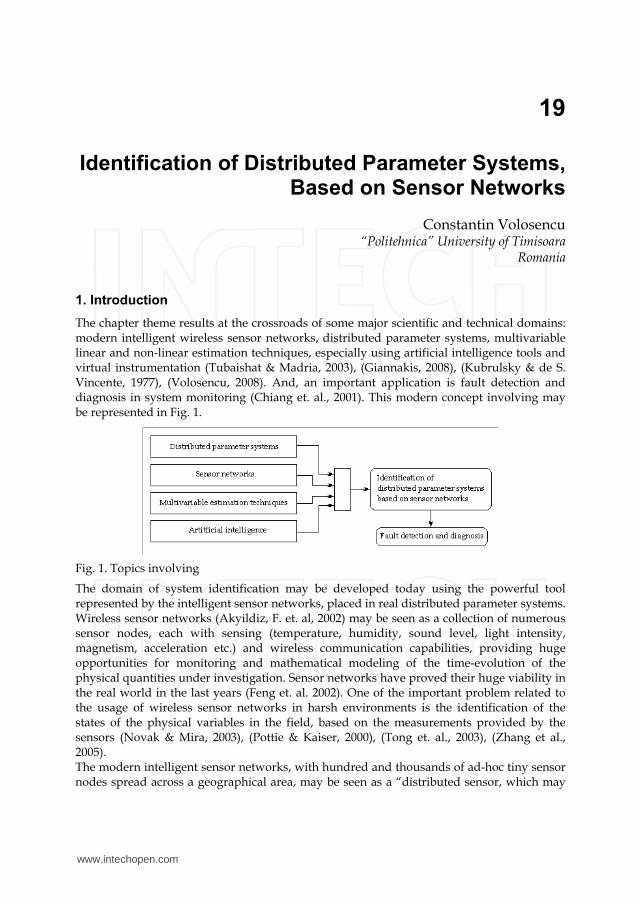
The chapter theme results at the crossroads of some major scientific and technical domains: modern intelligent wireless sensor networks, distributed parameter systems, multivariable linear and non-linear estimation techniques, especially using artificial intelligence tools and virtual instrumentation (Tubaishat & Madria, 2003), (Giannakis, 2008), (Kubrulsky & de S. Vincente, 1977), (Volosencu, 2008). And, an important application is fault detection and diagnosis in system monitoring (Chiang et. al., 2001). This modern concept involving may be represented in Fig. 1.

Fig. 1. Topics involving

The domain of system identification may be developed today using the powerful tool represented by the intelligent sensor networks, placed in real distributed parameter systems. Wireless sensor networks (Akyildiz, F. et. al, 2002) may be seen as a collection of numerous sensor nodes, each with sensing (temperature, humidity, sound level, light intensity, magnetism, acceleration etc.) and wireless communication capabilities, providing huge opportunities for monitoring and mathematical modeling of the time-evolution of the physical quantities under investigation. Sensor networks have proved their huge viability in the real world in the last years (Feng et. al. 2002). One of the important problem related to the usage of wireless sensor networks in harsh environments is the identification of the states of the physical variables in the field, based on the measurements provided by the sensors (Novak & Mira, 2003), (Pottie & Kaiser, 2000), (Tong et. al., 2003), (Zhang et al., 2005). The modern intelligent sensor networks, with hundred and thousands of ad-hoc tiny sensor nodes spread across a geographical area, may be seen as a “distributed sensor, which may

www.intechopen.com

New Trends in Technologies: Control, Management, Computational Intelligence and Network Systems

370

be placed in the field of the distributed parameter systems. The sensor network, as a “distributed sensor”, allows the usage of multivariable estimation techniques, in different ways: classical linear methods of modeling or methods based on artificial intelligence for complex non-linear systems. As smart and small devices the modern sensors are capable to be implemented in large distributed parameter systems. As an example of distributed parameter system with large application in practice the process of heat conduction is presented. Other applications are presented in literature (Rosculet & Craiu, 1979), (Basmadjian, 1999). The identification techniques (Ucinski, 2004), (Banks & Kunish, 1989), (Sjoberg, et. al., 1997), (Zhu et. al., 2007) are useful for applications ranging from control systems, fault detection and diagnosis, signal processing to time-series analysis. The artificial intelligence tools (Chairez et al., 2009), (Jassar et. al., 2009) may be used for identification of nonlinear complex systems as the distributed parameter systems are. ANFIS (Roger Jang, 1993), (Depari et. al., 2005), (Hou & Li, 2006), (Mellit et. al., 2007) as a method for non-linear system identification is a powerful tool to estimate future behavior in distributed parameter systems from acquired data obtained using wireless sensor connected in a distributed network placed in the field. The chapter presents a short survey of some results obtained in the study of using of sensor networks with multivariable estimation techniques for distributed parameter system identification. Sensor network topics, sensor network architectures and sensor network applications are presented. Starting from the measurements collected by the sensor nodes inside an investigated distributed parameter systems, this chapter offers an efficient methodology for identification with linear and non-linear time series. Some estimation algorithms and a method for monitoring distributed parameter systems based on sensor networks and the adaptive-network-based fuzzy inference scheme are presented (Volosencu, 2010). The chapter presents an application of a multivariable auto-regression estimation technique for estimation of heat transfer in space. A case study of temperature flow for a parabolic equation is analysed, based on these approach. Limited resources in terms of computational power, energy, memory and bandwidth impose heavy constraints on functionality of an effective malfunction detection system. For this reason these algorithms are designed and suitable for execution on the base station level and, by this, it is appropriate even for large-scale sensor networks. Sensor networks have proved their huge viability in the real world, being just a matter of time until this kind of networks will be standardized and used broadly in the field.

2. Sensor networks

Wireless sensor networks are extremely distributed systems having a large number of independent and interconnected sensor nodes, with limited computational and communicative potential. The sensors are deployed for data acquisition purposes on a wide range of locations, sometimes in resource-limited and hostile environments such as disaster areas, seismic zones, ecological contamination sites and other. In this structure data processing is at the sensor level, data transmission is wireless, sensing mechanism is not necessarily power supply is not necessarily wireless. Sensor network applications include: environmental monitoring, civil infrastructure monitoring, shared resource utilization, tracking, perimeter protection and surveillance. Application are in micro-climates, air quality, soil moisture, animal tracking, energy usage,

www.intechopen.com


371

office comfort, wireless thermostats, wireless light switches. In techniques they have as applications data acquisition of physical and chemical properties, at various spatial and temporal scales, as in distributed parameter systems, for automatic identification, measurements over long period of time. The sensor networks are deployed for data acquisition purposes on a wide range of locations, in resource-limited and hostile environments such as disaster areas, seismic zones, ecological contamination sites. All applications are distributed parameter systems. The modern sensors are smart, small, lightweight and portable devices, with a communication infrastructure intended to monitor and record specific parameters like temperature, humidity, pressure, wind direction and speed, illumination intensity, vibration intensity, sound intensity, power-line voltage, chemical concentrations and pollutant levels at diverse locations. The sensor number in a network is over hundreds or thousands of ad hoc tiny sensor nodes spread across different area. Thus, the network actively participates in creating a smart environment. They are low cost and low energy devices, realized in nanotechnology. With them we may developed low cost wireless platforms, including integrated radio and microprocessors. The sensors are adequate for autonomous operation in highly dynamic environments as distributed parameter systems. We may add sensors when they fail. They require distributed computation and communication protocols. They assure scalability, where the quality can be traded for system lifetime. They assure Internet connections via satellite. The structure of a modern sensor (Akyildiz, F. et. al, 2002), (Pottie & Kaiser, 2000), (Tubaishat & Madria, 2003) is presented in Fig. 2.

Fig. 2. The structure of a modern sensor

The dimension of such a sensor is comparable with a small coin. The sensors are characterized by: a robust radio technology, cheap and energy efficient processors, lifetime energy source, on-board memory, flexible I/O for various sensors, common highly available components, efficient resource utilization – currently uses 10 µA average, high modularity, flexible open source platform. Some examples of technical data are: 128 KB instruction EEPROM, 4 KB data EEPROM, 512 KB External Flash Memory, radio with 38 K or 19 K baud, at 900MHz, LEDs, µP at 7,3 MHz, JTAG, programming board, ISM Bands: 433-434,8 MHz Europe, power consumption: 16 mA Tx, 9 mA Rx, 2 µA sleep, transmission range: 1m, off the floor 100m range, ground level 10 m range, interface block data to laptop, GPS, cost: $ 95. Sensor are developed to measure: temperature, humidity, pressure, wind direction and speed, illumination intensity, vibration intensity, sound intensity, acceleration, power-line voltage, chemical concentrations and pollutant levels at diverse locations and others. All are variables in distributed parameter systems.

www.intechopen.com


372

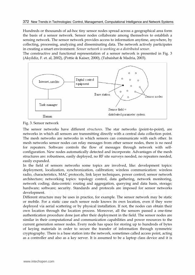
Hundreds or thousands of ad-hoc tiny sensor nodes spread across a geographical area form the basis of a sensor network. Sensor nodes collaborate among themselves to establish a sensing network. The sensor network provides access to information anytime, anywhere, by collecting, processing, analyzing and disseminating data. The network actively participates in creating a smart environment. Sensor network is working as a distributed sensor. The constructive and functional representation of a sensor network is presented in Fig. 3 (Akyildiz, F. et. al, 2002), (Pottie & Kaiser, 2000), (Tubaishat & Madria, 2003).

Fig. 3. Sensor network

The sensor networks have different structures. The star networks (point-to-point), are networks in which all sensors are transmitting directly with a central data collection point. The mesh networks are networks in which sensors can communicate with each other. In mesh networks sensor nodes can relay messages from other sensor nodes, there is no need for repeaters. Software controls the flow of messages through network with self-configuration. New nodes automatically detected and incorporate. Advantages of the mesh structures are: robustness, easily deployed, no RF site surveys needed, no repeaters needed, easily expanded. In the field of sensors networks some topics are involved, like: development topics: deployment, localization, synchronization, calibration; wireless communication: wireless radio, characteristics, MAC protocols, link layer techniques, power control; sensor network architecture; networking topics: topology control, data gathering, network monitoring, network coding; data-centric: routing and aggregation, querying and data basis, storage; hardware; software; security. Standards and protocols are imposed for sensor networks development. Different structure may be uses in practice, for example. The sensor network may be static or mobile. For a static case each sensor node knows its own location, even if they were deployed via aerial scattering or by physical installation. If not, the nodes can obtain their own location through the location process. Moreover, all the sensors passed a one-time authentication procedure done just after their deployment in the field. The sensor nodes are similar in their computational and communication capabilities and power resources to the current generation sensor nodes. Every node has space for storing up to hundreds of bytes of keying materials in order to secure the transfer of information through symmetric cryptography. There is a base station into the network, sometimes called access point, acting as a controller and also as a key server. It is assumed to be a laptop class device and it is

www.intechopen.com


373

supplied with long-lasting power. An example of a wireless cellular network architecture is presented in Fig. 4.

Fig. 4. Cellular network architecture

In this architecture, a number of base stations are already deployed within the field. Each base station forms a cell around itself that covers part of the area. Mobile wireless nodes and other appliances can communicate wirelessly, as long as they are within the area covered by one cell. A versatile architecture is a sensor network with mobile access is presented in Fig. 5.

Fig. 5. A sensor network with mobile access

This structure used for large-scale sensor networks. The main difference related to the cellular network architecture is that base stations are considered to be mobile, so each cell has varying boundaries which implies that mobile wireless nodes and other appliances can communicate wirelessly, as long as they are at least within the area covered by the range of the mobile access point. Multiple sensor nodes can detect an event situated in the surrounding area, so redundancy of sensor networks is assured. In the next paragraph we presents some examples of such distribute parameter systems with their mathematical models with partial derivative equations. The space model of the sensor deployed in the field with the heat sources is presented in Fig. 6.

www.intechopen.com


374

Fig. 6. Sensor deployment

The sensor SA measures the temperature θA in a point in this space. ,j kinP is the input power

in the point and ,j koutP is the output power from the point.

A Crossbow sensor network was used in practice, as it is presented in Fig. 7.

Fig. 7. The sensor network with mobile access

It has the following components: a starter kit, a MICA2 2,4 GHz wireless module, and an MTS320 sensor board. Their nodes are 2 MICAz 2,4 GHz modules, with 2 sensors MTS400, which are measuring temperature, humidity, pressure, ambient light intensity; 1 MICAz 2,4 GHz with 2 sensors MTS310 and 1 module MICAz 2,4 GHz working as a central node when it is connected through the UB port. A gateway MIB520 for node programming and a data acquisition board MDA320 with 8 analogue channels are provided. The network has the following software: MoteView for history sensor network monitoring and real time graphics and MoteWorks for nod programming in MesC language. The user interface allows some facilities, as: administration, searching, connections options and so on.

www.intechopen.com


375

This modern wireless sensor network has multiple measuring capabilities. So, it can measure temperature, humidity, light intensity or acceleration on 2 axes. For these kind of physical variables the mathematical models are as follows. For temperature:

2 2

2 2( , , )a Q x y t

t x y

θ θ θ⎛ ⎞∂ ∂ ∂= + +⎜ ⎟⎜ ⎟∂ ∂ ∂⎝ ⎠ (1)

where Q is the time variable source of heating, positioned in space and θ is the temperature. For light intensity:

2 2

( )I

E xh x

= + , ES

ΔΦ= Δ , 2

.S

I Ir

αΔΔΦ = = Δ (2)

where I is the luminous intensity of the light source, at the distance x and high h, as a measure of the source intensity as seen by the eye, E is the luminance at the specific point, defined as a ratio, with ΔΦ representing the flux that strikes a tiny area ΔS, calculated

considering a spherical surface of radius r, with Δα representing the solid angle. For acceleration:

, , ,yx

x y x y

dv dydv dxa a v v

dt dt dt dt= = = = (3)

where the above notations represents the acceleration ax, ay, the speed vx, vy and the space x, y on two axis for an object of the mass m, under a force F. Some characteristics measured for the sensor network are presented in Fig. 8.

Fig. 8. Temperature aand humidity transient characteristics

Redundancy is an inherent feature of sensor networks that is verified in practice and it is improving important aspects of their functioning (Curiac et. al., 2009).

www.intechopen.com


376

3. Distributed parameter systems

The distributed parameter systems, opposed to the lumped parameter systems, are systems whose state space is infinite dimensional. An object whose state is heterogeneous has distributed parameters. Such a system is described by partial differential equations. Partial differential equations are used to formulate problems involving functions of several variables, such as the propagation of sound or heat, electrostatics, electrodynamics, fluid, flow, elasticity. Distinct physical phenomena have identical mathematical formulations, and the same underlying dynamic governs them. One of the most important domain of applications of the partial differential equations is the process of heat conduction, with propagation of heat in anisotropic medium: propagation of heat in a porous medium, transference of heat in semi-space compound by two materials submitted to heating, processes of transference of heat between a solid wall and a flow of hot gas, estimation of the temperature field in space with fissured zone having the form of a circular disc. Applications related to electricity domain are: the propagation of electric current in cables, the heating of the electrical contacts. In the field of motion of fluid there are: plane motion of viscous fluids, running of viscous fluids in rectilinear tube, computation of losses of non-stationary heat in subterranean pipe, running of gases in water main. The processes of cooling and drying: cooling of clap, cooling of a sphere, drying of wood pieces, drying in vacuum. Phenomenon of diffusion: diffusion flow in a heavy sphere for chemical reactions happening with finite spit on the sphere surface, the flames diffusion, which appears to the beginning of a tube, repartition density of particles loading by the meteorites. Other applications are: estimation of the ice height covering the snow the arctic seas, motion of underground waters, alloy of heavy fusible particles, investigation of the wave close to the single point of the board of a plane plate, the growing of the gas particles in a fluid, substances combustion, the temperature modification in the air mass. (Rosculet & Craiu, 1979), (Basmadjian, 1999).

3.1 Process of heat conduction

Let it be an object of a volume 3V R⊂ . The frontier of dominium V is a surface S, formed by

a finite number of smooth surfaces. Let it be θ(P, t) the function of the object’s temperature,

at the time moment t, where P∈V is a point in the volume V. If different points of object

have different temperatures, θ(P, t)≠ct., then a heat transfer will take place, from the warmer

parts to the less warm parts. Let it be a regular surface σ placed in V, which contains the

point P. From the theory of thermal conductivity through the dσ in the time dt a heat

quantity dQ is passing, proportional to the product dσ.dt and proportion to the function

θ(P,t) derivative, along the normal n to the surface σ in the point P:

( , )P t

dQ k dtdn

θ σ∂= ∂ (4)

where k is a proportionality factor, called coefficient of internal thermal conductivity of the

object. The vector grad θ has its direction along the normal at the level surface for θ=ct., in

the sense of θ rising.

The law of heat propagation through an object in which there are no heat sources:

www.intechopen.com


377

k k kt x x y y z z

θ θ θ θγρ ⎛ ⎞∂ ∂ ∂ ∂ ∂ ∂ ∂⎛ ⎞ ⎛ ⎞= + +⎜ ⎟⎜ ⎟ ⎜ ⎟⎜ ⎟∂ ∂ ∂ ∂ ∂ ∂ ∂⎝ ⎠ ⎝ ⎠⎝ ⎠ (5)

The heat sources in the object have a distribution given by the function:

( , ) ( , , , )F t P F t x y z= (6)

If the object is homogenous / / .a k ctγ ρ= = and the equation (2) is written:

2

1

t x x y y z za

θ θ θ θ⎛ ⎞∂ ∂ ∂ ∂ ∂ ∂ ∂⎛ ⎞ ⎛ ⎞= + +⎜ ⎟⎜ ⎟ ⎜ ⎟⎜ ⎟∂ ∂ ∂ ∂ ∂ ∂ ∂⎝ ⎠ ⎝ ⎠⎝ ⎠ (7)

In the case of heat propagation through a bar:

( , )k F t xt x x

θ θγρ ∂ ∂ ∂⎛ ⎞= +⎜ ⎟∂ ∂ ∂⎝ ⎠ (8)

The initial conditions or of the limit conditions have physical significance. The equation

( ) ( , )div k grad F t Pt

θργ θ∂ = +∂ (9)

does not determine completely the state of the object K. We must take in considerations the initial state of the object, the temperature distribution in the object at the moment t=0:

0

( , , , ) ( , , )t

x y z t f x y zθ = = (10)

called initial conditions.

3.2 Discrete approximation We may associate to the equation (5) a system with finite differences. For this purpose the space S is divided into small pieces of dimension lp:

/pl l n= (11)

In each small piece Spi,j, i=1,…,n, j=1,…,n of the space S the temperature could be measured at each moment tk in a characteristic point Pi,j(xi, yj), of coordinate xi and yj. Let it be θi,jk the temperatures in the point Pi,j(xi, yj) at the moment tk. It is a general known method to approximate the derivatives of a variable with small variations. In the equation with partial derivatives there are derivatives of first order, in time, and derivatives of second order in space. So, theoretically, we may approximate the temperature derivative in time with a small variation in time, with the following relation:

-

-

1 1, ,

1

k ki j i j

k kt t t

θ θθ + +

+∂ =∂ (12)

Also, we may approximate the summation of the temperature second derivatives in space, with small variations in space and to obtain the following relations:

www.intechopen.com


378

-2 2

1, , 1, , 1 , 1

2 2 2

4i i i i ii j i j i j i j i j

px y l

θ θ θ θ θθ θ − + − ++ + +∂ ∂+ =∂ ∂ (13)

We may consider the temperature is measured as samples at equal time intervals with the

value

1k kh t t+= − (14)

called sample period, in a sampling procedure, with a digital equipment.

Combining the equations (6, 7, 8, 9) in the equation (1) a system with differences results:

( )1, , 1, , 1, , 1 , 12

4k k k k k k ki j i j i j i j i j i j i j

p

ah

lθ θ θ θ θ θ θ+ − + − += + + − + + + (15)

The sampling period h may be chosen according to different theories for signal sampling.

For example, we must choose it without obtaining alias errors at specific frequencies. In

practice the sampling period is taken according to the capacity of digital equipment to

manipulate data, the time constants of the system, assuring the conditions of stability,

controllability and observably for the discrete time model.

An interesting value for h is proposed in (Rosculet & Craiu, 1979) to eliminate the term θi,jk:

2

4

plh

a= (16)

so:

( )1, 1, 1, , 1 , 1

1

4k k k k ki j i j i j i j i jθ θ θ θ θ+ − + − += + + + (17)

The relation (17) gives a discrete approximation of temperature value θi,jk in every

characteristic points Pi,j of the space S, for i, j =1, …, n, at the every moment tk, k>1, from the

temperature values θi-1,jk-1, θi,j-1k-1, θi+1,jk-1 and θi,j+1k, at the antecedent moment tk-1, k-1>0, of

the adjacent points Pi-1,j, Pi,j-1, Pi+1,j and Pi,j+1.

Relations of the approximation error and for stability are given in literature (Rosculet &

Craiu, 1979).

The approximation (17) is a linear system with differences of nxn order.

In the discrete model (17) we must take in consideration the position points Piq,jq in the

discrete space of the sources Qiq,jqk at each time moment.

For transversal heat transfer from the surroundings the term transversal heat transfer from

the surroundings qm(θext-θ) must be added, where qm is the convective heat transfer

coefficient and θext is the external temperature. In the discrete model we must take account

on each point with a contact with the exterior: qm(θext i,jk-θi,jk) at each time moment.

3.3 Mathematical models

The distributed parameter systems have general mathematical models in continuous time

and space as partial differential equation, of parabolic form, as:

www.intechopen.com


379

1 2 3( )c c c Qt

θ θ θ∂ = ∇ ∇ + +∂ (18)

where the variables θ(ζ, t) are depending on time t≥0 and on space ζ∈V, where ζ is x for one axis, (x, y) for two axis or (x, y, z) for three axis, c1, c2 and c3 are coefficients, which could be also time variant and Q(ζ, t) is an exterior excitation, variable on time and space. So, in the general case, an implicit equation may be written:

2

2, , ,... 0f

t

θ θ θζ ζ

⎛ ⎞∂ ∂ ∂ =⎜ ⎟⎜ ⎟∂ ∂ ∂⎝ ⎠ (19)

For the partial differential equations some boundary conditions may be imposed to establish a solution. So, when the variable value of the boundary is specified there are Dirichlet conditions:

4c qθ = (20)

And, when the variable flux and transfer coefficient are specified there are Neumann conditions:

5 6 0c cθ θ∇ + = (21)

In the practical application case studies limits and initial conditions of the equation are imposed:

0(0, ) , [0, ], ( ,0) 0, [0, ],

( , ) , [0, ]l

t t T l

l t t T

ζζ

θ θ θ ζ ζθ θ

= ∈ = ∈= ∈ (22)

A system with finite differences may be associated to the equations. For this purpose the space S is divided into small pieces of dimension lp. In each small piece Spi, i=1,…,n of the space S the variable θ could be measured at each moment tk, using a sensor from the sensor network, in a characteristic point Pi(ζi), of

coordinate ζi. Let it be θik the variable value in the point Pi(ζi) at the moment tk. It is a general known method to approximate the derivatives of a variable with small variations. In the equation with partial derivatives there are derivatives of first order, in time, and derivatives of first and second order in space. For the parabolic equation a linear approximate system of derivative equations of first degree may be used:

d

A BQdt

Ψ = Ψ + (23)

where, this time, ψ is a vector containing the values of the variable θ(ζ, t) in different points of the space and at different time moments. Combining the equations a system of equations with differences results for the parabolic equation:

-1

1 1( , , , ) 0k k k kp i i i if θ θ θ θ+ + = (24)

www.intechopen.com


380

Taking account of equations (14, 15) it is obvious that several estimation algorithms may be developed as follows, based on the discrete models of the partial derivative equations.

4. Identification techniques

System identification is for building accurate, simplified models of complex systems from

noisy time-series data. It provides tools for creating mathematical models of dynamic

systems based on observed input/output data. The identification techniques are useful for

applications ranging from control system design and signal processing to time-series

analysis. Actually, there is a huge amount written on the subject of system identification.

But only the experience with real data may help us to understand more. It is important to

remember that any estimated model, no matter how good it looks on design, has only

picked up a simple reflection of reality. So, in this aspect the sensor network is the powerful

tool. The identification techniques are useful for applications ranging from control systems,

fault detection and diagnosis, signal processing to time-series analysis. There are

identification methods based on parametric model and on nonparametric models. There are

identification methods based on parametric model and on nonparametric models. The

general system identification block diagram is presented in Fig. 9.

Fig. 9. Identification signals

The signals involved on a process for identification and its model are: the inputs u(t), the errors e(t), the outputs y(t) and the estimated outputs. A simple estimation of the variable value at the moment tk+1 from the values of the adjacent

sensors may be done using the above relations and adjacent sensor placed in space. To

obtain an identification model for the process in theory and practice there are methods for

model identification dedicated to linear or nonlinear systems, or based on artificial

intelligence tools as fuzzy logic or neural networks.

4.1 Linear models

For linear systems the most known methods are for the general case with the Box-Jenkins

model with some special cases as the ARMAX model – the auto-regression and a moving

average of white noise with the simplification of the ARX model. With the ARX model it is

possible to predict what the system output - the temperatures in the points of the space will

be 1, 1

ˆ ( )ki j ktθ + + , based on measurements of the input Q(x, y, t) –the heat generated by an

external source and the antecedent and adjacent outputs 11, 1( )k

i j k ltθ −− − − , where l=1,2,… We may apply this method in all the points of the network, considering the boundary

conditions as inputs and the value in the point as an output.

www.intechopen.com


381

Also, we may use an autoregressive model in an autoregressive predictor. An autoregressive (AR) model may approximate the time evolution of the measured values provided by each sensor. This kind of systems evolves due to its "memory", generating internal dynamics. The AR model definition for temperature in the space is as follows:

-1 1 1

, 1 1 , ,ˆ ˆ ˆ( ) ( ) ... ( ) ( )k k ki j k i j k n i j k nt a t a t tθ θ θ ξ+ + ++ = + + + (25)

where 1, 1

ˆ ( )ki j ktθ + + is the temperature series under investigation, the series of values

measured by the same sensor, ia are the auto regression coefficients, n is the order of the

auto regression and ξ is the noise which is almost always assumed to be a Gaussian white

noise. By convention the time series is assumed to be zero mean. If not, another term (a0) is

added in the right member of equation. The ai coefficients may be also time-varying:

-1 1 1

, 1 1 , ,ˆ ˆ ˆ( ) ( ) ( ) ... ( ) ( ) ( )k k ki j k i j k n i j k nt a t t a t t tθ θ θ ξ+ + ++ = + + + (26)

Based on the model we may either estimate the coefficients ai(t) in case that the time series

, ( )ki j ktθ , -

-1

, 1( )ki j ktθ , …, -

-, ( )k ni j k ntθ is known (recursive parameter estimation), either predict

future value 1, 1

ˆ ( )ki j ktθ + + in case that ai(t) coefficients and the past values , ( )k

i j ktθ , --

1, 1( )k

i j ktθ ,

…, --, ( )k n

i j k ntθ are known (AR prediction).

4.2 Adaptive-network-based fuzzy inference

In the tentative of identification of distributed parameter systems using sensor networks and fuzzy logic as a tool of artificial intelligence we must make the following steps: 1. Starting from a primary mathematic model of distributed parameters system - an equation with partial derivatives. 2. Defining system real variables. 3. Choosing of universe of discourse for system variables. 4. Choosing the fuzzy variables for the system and their fuzzy values on the universes of discourse. 5. Choosing the membership function to describe the fuzzy values. 6. Developing the rule base for inference, considering the operator experience working with the distributed parameter system. 7. Choosing the inference method. 8. Choosing the defuzzification method. 9. Developing a fuzzy system to model the distributed parameter system. 10. Comparing the primary mathematic model with the fuzzy model after the simulation and errors determination. As it was presented above the description of distributed parameter systems is done with mathematical models with real variables u(t, x, y, z), in a 3 dimensional Cartesian coordinate

system with the origin (xo, y0, z0), for time t≥0. The equation with partial derivatives is (5). We may do a fuzzy modeling for this system. The variables are defined on the following universe of discourse:

0 0

0

[ , ], [ , ]

[ , ], [ , ]

x M y M

z M v m M

x U x x y U y y

z U z z v U v v

∈ = ∈ =∈ = ∈ = (27)

The fuzzy variables for space are taken the following fuzzy values: ZE, PS, PM, PB, PVB. The system variables, if they have symmetric values face to 0 may take the following fuzzy

www.intechopen.com


382

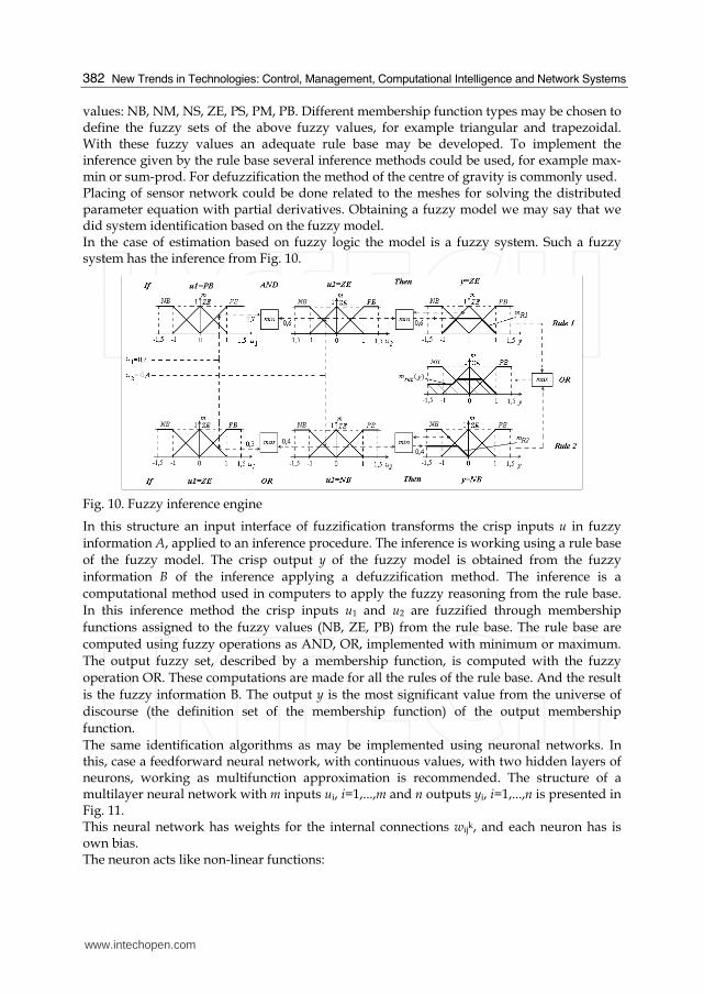
values: NB, NM, NS, ZE, PS, PM, PB. Different membership function types may be chosen to define the fuzzy sets of the above fuzzy values, for example triangular and trapezoidal. With these fuzzy values an adequate rule base may be developed. To implement the inference given by the rule base several inference methods could be used, for example max-min or sum-prod. For defuzzification the method of the centre of gravity is commonly used. Placing of sensor network could be done related to the meshes for solving the distributed parameter equation with partial derivatives. Obtaining a fuzzy model we may say that we did system identification based on the fuzzy model. In the case of estimation based on fuzzy logic the model is a fuzzy system. Such a fuzzy system has the inference from Fig. 10.

Fig. 10. Fuzzy inference engine

In this structure an input interface of fuzzification transforms the crisp inputs u in fuzzy information A, applied to an inference procedure. The inference is working using a rule base of the fuzzy model. The crisp output y of the fuzzy model is obtained from the fuzzy information B of the inference applying a defuzzification method. The inference is a computational method used in computers to apply the fuzzy reasoning from the rule base. In this inference method the crisp inputs u1 and u2 are fuzzified through membership functions assigned to the fuzzy values (NB, ZE, PB) from the rule base. The rule base are computed using fuzzy operations as AND, OR, implemented with minimum or maximum. The output fuzzy set, described by a membership function, is computed with the fuzzy operation OR. These computations are made for all the rules of the rule base. And the result is the fuzzy information B. The output y is the most significant value from the universe of discourse (the definition set of the membership function) of the output membership function. The same identification algorithms as may be implemented using neuronal networks. In this, case a feedforward neural network, with continuous values, with two hidden layers of neurons, working as multifunction approximation is recommended. The structure of a multilayer neural network with m inputs ui, i=1,...,m and n outputs yi, i=1,...,n is presented in Fig. 11. This neural network has weights for the internal connections wijk, and each neuron has is own bias. The neuron acts like non-linear functions:

www.intechopen.com


383

Fig. 11. Neural network structure

1

1

m

i a ji j ij

v f w u b=

⎛ ⎞⎜ ⎟= +⎜ ⎟⎝ ⎠∑ (28)

where fa is the activation function. Such activation function are the sigmoid th(x) for the

neurons from the hidden layers from the interior of the neural network and the linear

function y=x, for the neurons from the output layer. The neural network transfer function is:

2q q q 1q q2kj jii j jk k

kj qi q

E= - = S ( ) =w w h u u

wη η ηδ δ∂ ′Δ ∂ ∑ ∑ (29)

The neural identification has the block diagram from Fig. 12.

Fig. 12. Direct neural identification

In this case the model is a neural network. The neural model is obtained by training (learning) the neural network with training sets (ui, yi), i=1, N, obtained from real measurements from the distributed parameter systems, achieved using sensor networks. A cost function is imposed for training.

- 21( ) ( ) , 1,...,

2q qdi i

qi

E w y y i p= =∑ (30)

A training method, based on error backpropagation is used. For example the Levenberg

Marquard method, using a cvasi-Newton method to minimize the cost function assures the

small number of iterations to obtain the appropriate weight and biases values. A rule of

weight updating is applied:

www.intechopen.com


384

qi

( )2q q q2 1q qi ji j kkj j k

kj qqi

Ew S h u= - = =w u

wδη η η δ∂ ′∑Δ ∂ ∑ (31)

As we said above, a supervised learning (by backpropagation) is used to obtain the best values of the unknown weights w and biases b, propagating back through the network the training output error

ˆe y y= − (32)

computing the gradient ΔE. An example of training error for backpropagation with the Levenberg Marquardt method is presented in Fig. 13.

Fig. 13. Traning error

The neural network developed in the neuro-fuzzy modeling frame has the following general structure. If the sum-prod inference is used a neural structure with product between the activation function outputs and weights and summation of the connections signals may be developed. The first layer is the input layer. The second layer represents the input membership or fuzzification layer. The neurons represent fuzzy sets used in the antecedents of fuzzy rules determine the membership degree of the input. The activation function represents the membership functions. The 3rd layer represents the fuzzy rule base layer. Each neuron corresponds to a single fuzzy rule from the rule base. The inference is in this case the sum-prod inference method, the conjunction of the rule antecedents being made with product. The weights of the 3rd and 4th layers are the normalized degree of confidence of the corresponding fuzzy rules. These weights are obtained by training in the learning process. The 4th layer represents the output membership function. The activation function is the output membership function. The 5th layer represents the defuzzification layer, with single output, and the defuzzification method is the center of gravity.

4.3 Algorithms and method

The application is using the following algorithms, obtained from the above general discretization function.

www.intechopen.com


385

Estimation algorithm 1. It estimates the value of the variable 1kiθ + at the moment tk+1,

measuring the values of the variables -1 1, ,k k ki i iθ θ θ+ at the anterior moment tk:

( )-1

1 1 1, ,k k k ki i i ifθ θ θ θ+ += (33)

This is a multivariable estimation algorithm, based on the adjacent nodes [9].

Estimation algorithm 2. It estimates the value of the variable 1kiθ + at the moment tk+1,

measuring the values of the same variable - - -1 2 3, , ,k k k ki i i iθ θ θ θ , but at four anterior moments tk,

tk-1, tk-2 and tk-3.

( )- - -1 1 2 32 , , ,k k k k k

i i i i ifθ θ θ θ θ+ = (34)

4.4 Estimator mechanism

The estimators are linear and also non-linear. All are described by the function y=f(u1, u2, …, un), using the linear model and the adaptive-network-based fuzzy inference. The general structure is presented in Fig. 14.

Fig. 14. The estimator input-output general structure

The number of inputs depends on the estimation algorithm, on the specific position in space of the measuring points, on the conditions of determination. The linear estimation algorithm is obtained with the least square method. The ANFIS procedure is well known and it may use a hybrid learning algorithm to identify the membership function parameters of the adaptive system. A combination of least-squares and backpropagation gradient descent methods may be used for training membership function parameters, modeling a given set of input/output data.

4.5 The monitoring structure The structure of the estimation and decetion system is presented in Fig. 15.

Fig. 15. The monitoring structure

The measured values from sensors are memorized and a multivariable estimation algorithm is applied. Based on the error between the measured and estimated values a decision is taken. The error has the equation:

www.intechopen.com


386

- ˆ( ) ( ) ( )A A Ae t x t x t= (35)

This procedure has application in fault detection and diagnosis, with example in malicious detection of sensors. Such example is presented.

5. Method for monitoring

The following method is according to the objectives of monitoring of defined distributed parameter system from the practical application in the real world, as heat distribution, wave propagation. These systems have known mathematical model as a partial differential equation as a primary model from physics, with well-defined boundary and initial conditions for the system in practice. These represent the basic knowledge for a reference model from real data observation. The primary physical model must be discretized, to obtain a mathematical model as a multi input - multi output state space model. The unstructured meshes may be generated. The sensors must be placed in the field according to the meshes structured under the form of nodes and triangles. A scenario for practical applications could be chosen and simulated. The simulation and the practical measurements are producing transient regime characteristics. Those transient characteristics are due to the system dynamics in a training process. In steady state we cannot train the neural model. On these transient characteristics, seen as times series, the estimation algorithms may be applied. ANFIS is used to implement the non-linear estimation algorithms. With these algorithms future states of the process may be estimated. Possible fault in the system are chosen and strategies for detection may be developed, to identify and to diagnose them, base on the state estimation. In practice applying the method presumes the following steps: -placing a sensor network in the field of the distributed parameter system; -acquiring data, in time, from the sensor nodes, for the system variables; -using measured data to determine an estimation model based on ANFIS; -using measured data to estimate the future values of the system variables; -imposing an error threshold for the system variables; -comparing the measured data with the estimated values; -if the determined error is greater then the threshold a default occurs; -diagnosing the default, based on estimated data, determining its place in the sensor network and in the distribute parameter system field. The interpolation techniques may be used for spatial distributed system identification with wireless sensor networks (Volosencu & Curiac, 2009). Considering the continuous development of the wireless device technology, securing wireless sensor networks became more and more a significant task. One of the important problems that are related to the use of wireless sensor networks in harsh environments is the gap in their security. The strategy on time series predictors based on past and present values obtained from neighboring nodes from this chapter with its estimation algorithms is a basic for discovery of malfunctioning or attacked sensor nodes. Some strategies based on antecedent values provided by each sensor are presented for detecting their malicious activity in (Curiac et. al., 2007), (Curiac et. al., 2009), (Plastoi et. al., 2009).

6. Experimental results

In this chapter a parabolic case study consisting in a heat distribution flux through a plane square surface of dimensions l=1, with Dirichlet boundary conditions as constant temperature on three margins:

www.intechopen.com


387

h rθθ = (36)

with r=0, and a Neuman boundary condition as a flux temperature from a source

nk q gθ θ∇ + = (37)

where q is the heat transfer coefficient q=0, g=0, hθ=1.

The heat equation, of a parabolic type, is:

( ) ( )extC k Q ht

θθρ θ θ θ∂ = ∇ ∇ + + − (38)

where ρ is the density of the medium, C is the thermal (heat) capacity, k is the thermal

conductivity, coefficient of heat conduction, Q is the heat source, hθ is the convective heat

transfer coefficient, θext is the external temperature. Relative values are chosen for the

equation parameters: ρC=1, Q=10, k=1.

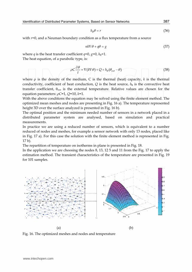
With the above conditions the equation may be solved using the finite element method. The

optimized mean meshes and nodes are presenting in Fig. 16 a). The temperature represented

height 3D over the surface analyzed is presented in Fig. 16 b).

The optimal position and the minimum needed number of sensors in a network placed in a

distributed parameter system are analysed, based on simulation and practical

measurements.

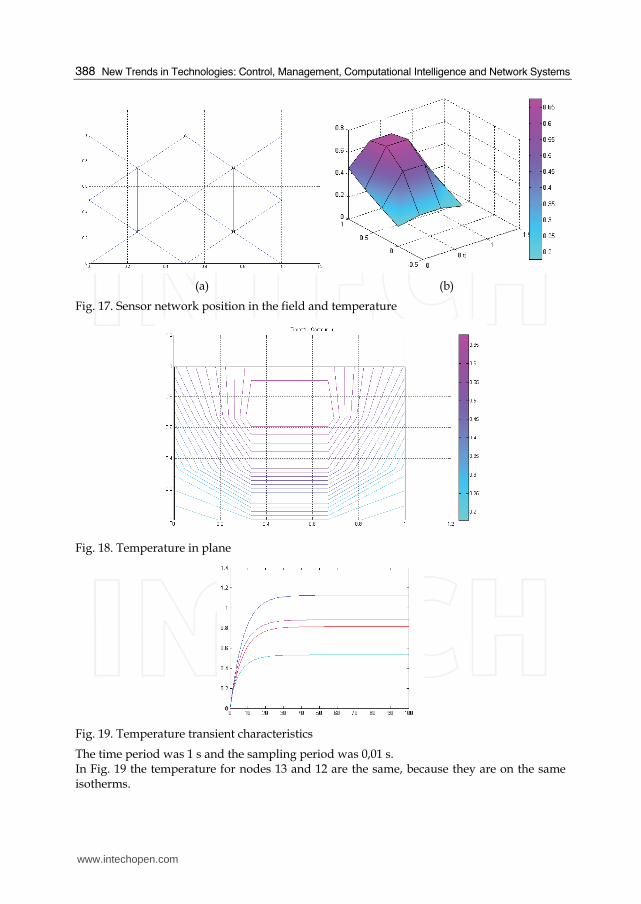
In practice we are using a reduced number of sensors, which is equivalent to a number

reduced of nodes and meshes, for example a sensor network with only 13 nodes, placed like

in Fig. 17 a). For this case the solution with the finite element method is represented in Fig.

17 b).

The repartition of temperature on isotherms in plane is presented in Fig. 18.

In the application we are choosing the nodes 8, 13, 12 5 and 11 from the Fig. 17 to apply the

estimation method. The transient characteristics of the temperature are presented in Fig. 19

for 101 samples.

(a) (b)

Fig. 16. The optimized meshes and nodes and temperature

www.intechopen.com


388

(a) (b)

Fig. 17. Sensor network position in the field and temperature

Fig. 18. Temperature in plane

Fig. 19. Temperature transient characteristics

The time period was 1 s and the sampling period was 0,01 s. In Fig. 19 the temperature for nodes 13 and 12 are the same, because they are on the same isotherms.

www.intechopen.com


389

We are chosen as an example the node 5 to be the node with the estimated temperature, based on the first recursive algorithm:

15 8 13 12 11( , , , )k k k k kfθ θ θ θ θ+ = (39)

And also for the node 5 we will apply the second algorithm, auto-recursive:

- - -1 1 2 35 5 5 5 5( , , , )k k k k kfθ θ θ θ θ+ = (40)

The fuzzy inference system structure is presented in Fig. 20.

Fig. 20. Fuzzy inference system

The comparison transient characteristics for training and testing output data are presented in Fig. 21. The average testing error is 2,017.10-5. Number of training epochs is 3. For the second algorithm the training error was of 0,007, number of epochs 3 and the testing error 0,007. The fuzzy inference system general structure is the same, but with different parameter values. The estimated output for the second algorithm is presented in Fig. 22.

Fig. 21. Comparison between training and testing output

www.intechopen.com


390

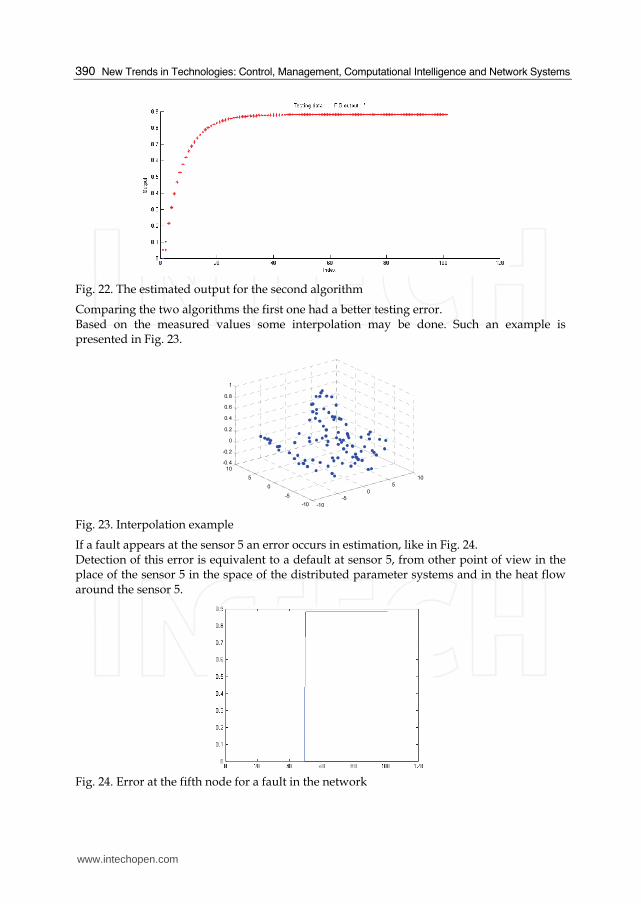
Fig. 22. The estimated output for the second algorithm

Comparing the two algorithms the first one had a better testing error. Based on the measured values some interpolation may be done. Such an example is presented in Fig. 23.

-10

-5

0

5

10

-10

-5

0

5

10

-0.4

-0.2

0

0.2

0.4

0.6

0.8

1

Fig. 23. Interpolation example

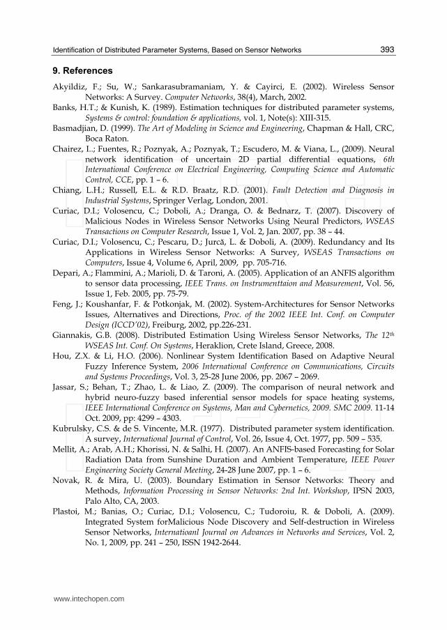
If a fault appears at the sensor 5 an error occurs in estimation, like in Fig. 24. Detection of this error is equivalent to a default at sensor 5, from other point of view in the place of the sensor 5 in the space of the distributed parameter systems and in the heat flow around the sensor 5.

Fig. 24. Error at the fifth node for a fault in the network

www.intechopen.com


391

For an example of the estimated temperature ˆˆ ( ) ( )A Ax t tθ= for the sensor SA is presented in

Fig. 25, over the original time series xA(t),

Fig. 25. Sensor value and the estimate

The error ˆ( ) ( ) ( )A A Ae t x t x t= − is presented in Fig. 26.

Fig. 26. Sensor error

We may see the error appearance at the time moment 400 s, caused by a fault at the node xA. The estimated signal follows the real signal after a small delay. Virtual instrumentation using National Instruments technology was used to implement the monitoring system. The virtual instrument for temperature measurement and estimation is presented in Fig. 27 a). The virtual instrument for temperature estimation error is presented in Fig. 27 b). The sample period was 9 s.

(a) (b)

Fig. 27. (a) Mesured and estimated temperature (b) Estimation error

www.intechopen.com


392

The validation of results is made based on a quadratic error criterion, which is taken account of all set i=1,…,n of measured data and estimates:

2

1

( )n

Aii

J e t=

=∑ (41)

7. Conclusion

This chapter presents some considerations on time series identification methodology using a wireless sensor network as a complex measurement system. After acquiring the measured values from the area covered by sensor networks, some estimation techniques may be applied. Some auto-regression estimation linear or ANFIS models may be developed. This methodology can be efficiently implemented on sensor network base stations, so there is no need for other hardware resources. A comparison of different identification methods is presented, in order to use the adaptive-network-based fuzzy inference. Some examples of generated meshes and temperature estimates for different numbers of sensor are presented. The main attention is given to the way of how to chose the number and the positions of the sensor nodes according to the desired accuracy in the identification process. The chapter presents two algorithms for estimation of state variables in distributed parameter systems of parabolic case. The algorithms are based on non-linear exogenous models with regression and auto-regression. Also, a method for monitoring distributed parameter systems based on these algorithms, sensor networks and ANFIS for non-linear system identification is presented. The sensor network is seen as a “distributed sensor”. The algorithms are based on regression using the values provided by the adjacent nodes of the sensor network and on autoregressive relation with the values from anterior time moments of the same node. The method described the way how to use all these concepts for fault detection and diagnosis in distributed parameter systems, using the measured values provided by the sensor and the estimated values computed by the ANFIS estimator, calculating an error and detecting the fault based on a decision taken after a threshold comparison. Estimations methods may be applied in the case of discovery of malicious nodes in wireless sensor networks. A case study for two algorithms are presented for parabolic type. A comparison between the algorithms is made. Good approximations were obtained. Developing of the algorithms and the method are taken in consideration in the future, in other applications, considering all the capabilities of the sensor nodes to measure physical variables. This approach allows treatment of large and complex systems with many variables by learning and extrapolation. An interesting application could be the monitoring of earth environment at low and high altitudes, based on new types of sensor networks specialized for this purpose. The implementation was made using virtual instruments of National Instruments technology.

8. Acknowledgement

This work was developed in the frame of PNII-IDEI-PCE-ID923-2009 CNCSIS - UEFISCSU grant.

www.intechopen.com


393

9. References

Akyildiz, F.; Su, W.; Sankarasubramaniam, Y. & Cayirci, E. (2002). Wireless Sensor Networks: A Survey. Computer Networks, 38(4), March, 2002.

Banks, H.T.; & Kunish, K. (1989). Estimation techniques for distributed parameter systems, Systems & control: foundation & applications, vol. 1, Note(s): XIII-315.

Basmadjian, D. (1999). The Art of Modeling in Science and Engineering, Chapman & Hall, CRC, Boca Raton.

Chairez, I..; Fuentes, R.; Poznyak, A.; Poznyak, T.; Escudero, M. & Viana, L., (2009). Neural network identification of uncertain 2D partial differential equations, 6th International Conference on Electrical Engineering, Computing Science and Automatic Control, CCE, pp. 1 – 6.

Chiang, L.H.; Russell, E.L. & R.D. Braatz, R.D. (2001). Fault Detection and Diagnosis in Industrial Systems, Springer Verlag, London, 2001.

Curiac, D.I.; Volosencu, C.; Doboli, A.; Dranga, O. & Bednarz, T. (2007). Discovery of Malicious Nodes in Wireless Sensor Networks Using Neural Predictors, WSEAS Transactions on Computer Research, Issue 1, Vol. 2, Jan. 2007, pp. 38 – 44.

Curiac, D.I.; Volosencu, C.; Pescaru, D.; Jurcă, L. & Doboli, A. (2009). Redundancy and Its Applications in Wireless Sensor Networks: A Survey, WSEAS Transactions on Computers, Issue 4, Volume 6, April, 2009, pp. 705-716.

Depari, A.; Flammini, A.; Marioli, D. & Taroni, A. (2005). Application of an ANFIS algorithm to sensor data processing, IEEE Trans. on Instrumenttaion and Measurement, Vol. 56, Issue 1, Feb. 2005, pp. 75-79.

Feng, J.; Koushanfar, F. & Potkonjak, M. (2002). System-Architectures for Sensor Networks Issues, Alternatives and Directions, Proc. of the 2002 IEEE Int. Conf. on Computer Design (ICCD’02), Freiburg, 2002, pp.226-231.

Giannakis, G.B. (2008). Distributed Estimation Using Wireless Sensor Networks, The 12th WSEAS Int. Conf. On Systems, Heraklion, Crete Island, Greece, 2008.

Hou, Z.X. & Li, H.O. (2006). Nonlinear System Identification Based on Adaptive Neural Fuzzy Inference System, 2006 International Conference on Communications, Circuits and Systems Proceedings, Vol. 3, 25-28 June 2006, pp. 2067 – 2069.

Jassar, S.; Behan, T.; Zhao, L. & Liao, Z. (2009). The comparison of neural network and hybrid neuro-fuzzy based inferential sensor models for space heating systems, IEEE International Conference on Systems, Man and Cybernetics, 2009. SMC 2009. 11-14 Oct. 2009, pp: 4299 – 4303.

Kubrulsky, C.S. & de S. Vincente, M.R. (1977). Distributed parameter system identification. A survey, International Journal of Control, Vol. 26, Issue 4, Oct. 1977, pp. 509 – 535.

Mellit, A.; Arab, A.H.; Khorissi, N. & Salhi, H. (2007). An ANFIS-based Forecasting for Solar Radiation Data from Sunshine Duration and Ambient Temperature, IEEE Power Engineering Society General Meeting, 24-28 June 2007, pp. 1 – 6.

Novak, R. & Mira, U. (2003). Boundary Estimation in Sensor Networks: Theory and Methods, Information Processing in Sensor Networks: 2nd Int. Workshop, IPSN 2003, Palo Alto, CA, 2003.

Plastoi, M.; Banias, O.; Curiac, D.I.; Volosencu, C.; Tudoroiu, R. & Doboli, A. (2009). Integrated System forMalicious Node Discovery and Self-destruction in Wireless Sensor Networks, Internatioanl Journal on Advances in Networks and Services, Vol. 2, No. 1, 2009, pp. 241 – 250, ISSN 1942-2644.

www.intechopen.com


394

Pottie, G.J. & Kaiser, W.J. (2000). Wireless Integrated Network Sensors. Communications of the ACM, vol. 43, 2000.

Roger Jang, J.S. (1993). ANFIS: Adaptive Network Based Fuzzy Inference Systems, IEEE Trans. on Systems, Man, and Cybernetics, Vol. 23, No. 03, May 1993, pp. 665-685.

Rosculet, M.N. & Craiu, M. (1979). Ecuatii diferentiale aplicative, Ed. Academiei RSR, Bucuresti, 1979.

Tong, L.; Zhao, Q. & Adireddy, S. (2003). Sensor Networks with Mobile Agents, Proceedings IEEE 2003 MILCOM, Boston, 2003, pp. 688-694.

Tubaishat, M. & Madria, S. (2003). Sensor networks: an overview, IEEE Potential, Apr. 2003, Vol. 22, Issue 2, pap. 20- 23.

Ucinski, D. (2004). Optimal Measurement Methods for Distributed Parameter System Identification, CRC Press, 2004.

Sjoberg, J., et. all. (1997). Non linear black box modeling in system identification: an unified overview, Automatica, 33, 1997, 1691-1724.

Volosencu, C. (2008). Identification of Distributed Parameter Systems, Based on Sensor Networks and Artificial Intelligence, WSEAS Transactions on Systems, Issue 6, Vol. 7, June 2008, pp. 785-801.

Volosencu, C. & Curiac, D.I. (2009). Interpolation Techniques for Spatial Distributed System Identification Using Wireless Sensor Networks, Recent Advances in Automation& Information, Proceedings of the 10th WSEAS Int. Conf. on Automation & Information (ICAI’09), Prague, March 23-25, 2009, pp. 383-376.

Volosencu, C. (2010). Algorithms for Estimation in Distributed Parameter Systems Based on Sensor Networks and ANFIS, WSEAS Transactions on Systems, Issue 3, Volume 9, March 2010, pp. 283-294, ISSN: 1109-2777.

Zhang H. et all. (2005). Estimation in sensor actuators arrays using reduced order physical models, 4th Int. Symp. Information Processing in Sensor Networks, Los Angeles, CA, 2005.

Zhu, Y.F.; Tan, H.Z.; Wan, P. & Zhang, Y. (2007). A blind approach to nonlinear system identification, IET Conference on Wireless, Mobile and Sensor Networks, 2007. (CCWMSN07). 12-14 Dec. 2007, pg. 209 – 212.

www.intechopen.com

New Trends in Technologies: Control, Management,Computational Intelligence and Network SystemsEdited by Meng Joo Er

ISBN 978-953-307-213-5Hard cover, 438 pagesPublisher SciyoPublished online 02, November, 2010Published in print edition November, 2010

InTech EuropeUniversity Campus STeP Ri Slavka Krautzeka 83/A 51000 Rijeka, Croatia Phone: +385 (51) 770 447 Fax: +385 (51) 686 166www.intechopen.com

InTech ChinaUnit 405, Office Block, Hotel Equatorial Shanghai No.65, Yan An Road (West), Shanghai, 200040, China

Phone: +86-21-62489820 Fax: +86-21-62489821

The grandest accomplishments of engineering took place in the twentieth century. The widespreaddevelopment and distribution of electricity and clean water, automobiles and airplanes, radio and television,spacecraft and lasers, antibiotics and medical imaging, computers and the Internet are just some of thehighlights from a century in which engineering revolutionized and improved virtually every aspect of human life.In this book, the authors provide a glimpse of the new trends of technologies pertaining to control,management, computational intelligence and network systems.

How to referenceIn order to correctly reference this scholarly work, feel free to copy and paste the following:

Constantin Volosencu (2010). Identification of Distributed Parameter Systems Based on Sensor Networks,New Trends in Technologies: Control, Management, Computational Intelligence and Network Systems, MengJoo Er (Ed.), ISBN: 978-953-307-213-5, InTech, Available from: http://www.intechopen.com/books/new-trends-in-technologies--control--management--computational-intelligence-and-network-systems/identification-of-distributed-parameter-systems-based-on-sensor-networks

Date post:	25-Aug-2018
Category:	Documents
Upload:	phamdan
View:	220 times
Download:	0 times

Identification of Distributed Parameter Systems, …cdn.intechopen.com/pdfs-wm/12315.pdf ·...

Documents