Page 1
Water and Environmental Engineering Department of Chemical Engineering
Identification of flood risk areas in an open storm-water system with MIKE URBAN –
Senai Town, Malaysia
Master’s Thesis by
Louise Reuterwall and Henrik Thorén
March 2009
Page 3
III
Vattenförsörjnings- och Avloppsteknik Institutionen för Kemiteknik Lunds Universitet
Water and Environmental Engineering Department of Chemical Engineering Lund University, Sweden
Identification of flood risk areas in an open storm-
water system with MIKE URBAN – Senai Town, Malaysia
Master Thesis number: 2009-04
Louise Reuterwall and Henrik Thorén Water and Environmental Engineering Department of Chemical Engineering
March 2009
Supervisor: Associate professor Karin Jönsson
Co-supervisor: Professor Dr. Zulkifli Yusop, UTM Malaysia
Co-supervisor: Henrik Sønderup, Rambøll Denmark
Examiner: Professor Jes la Cour Jansen
Picture on front page:
1. Main channel in the open storm-water system in Senai Town, Johor State, Malaysia. (L. Reuterwall)
Postal address: Visiting address: Telephone:
P.O. Box 124 Getingevägen 60 +46 46-222 82 85
SE-221 00 Lund +46 46-222 00 00
Sweden Telefax:
+46 46-222 45 26
Web address:
www.vateknik.lth.se
1
Page 5
V
List of abbreviations
CGCM1 – Coupled General Circulation Model
CRS – Cross Section
CSIRO – Commonwealth Scientific and Industrial Research Organisation
DEM – Digital Elevation Map
DHI – Danish Hydrological Institute
DMP – Drainage Master Plan
EPA – Environmental Protection Agency
ESRI – Environmental Systems Research Institute
GCM – Global Climate Model
GIS – Geographical Information System
IPASA – Institute of Environmental & Water Resource
IPCC – Intergovernmental Panel on Climate Change
MMD – Malaysia Meteorological Department
MASMA – Manual Saliran Mesra Alam Malaysia (Urban Stormwater Management Manual
For Malaysia)
MOUSE – Model for Urban Sewers
m.a.s.l. – Meter Above Sea Level
NAHRIM – National Hydraulic Research Institute of Malaysia
PVC – PolyVinylChloride (Plastic)
RDI – Rainfall Dependent Infiltration
SRES – Special Report on Emisson Scenarios
SUDS – Sustainable Urban Drainage Systems
SWMM – Storm-Water Management Model
ToC – Time of Concentration
UTM – Universiti Teknologi Malaysia
Page 7
VII
Summary By the year of 2020 Malaysia is prospected to become a developed nation due to twenty years
of rapid socio-economic growth. As strong urbanization will take place, runoff will increase
as a result of growth and spread of impervious surfaces. The study area in this project is in
Senai Town which is situated in an important economic centre in the mid-southern region of
Johor State in South-East Malaysia close to the border of Singapore. Flash floods, water
pollution and ecological damage are associated with storm water in Malaysia. To solve future
problems with flooding in the region, the Government of Johor carried out a Drainage Master
Plan (DMP) for Bandar Senai (DID, 2005a). The purpose of the DMP was to indentify
existing drainage problems and propose long-term improvements with a projected year of
2020. The objective of this study is to identify areas with risk of flooding today and in the
future.
A rainfall-runoff model was created in the computer program MIKE URBAN in order to
forecast the future situation in the drainage system. The necessary information to create the
model was taken from the DMP and collected from onsite observations. Quantitative data
such as rainfall and water level was recorded in order to perform a calibration of the model
during the 24th
of October to the 18th
of November 2008. The tributary Cabang Sungai Senai
Fasa 1 is the object of this study which has a catchment area of about 33 hectares and a length
of almost 1 kilometre. The drainage network is almost entirely an open drainage system and
consists of concrete lined channels and culverts of different dimensions. At low-lying areas in
the Sungai Senai catchment, flash floods have occurred in the past due to insufficient capacity
in the drainage system. Additional cause is the backwater effect from the river Sungai Skudai.
In the region of the study area the climate is tropical with an annual average temperature of
27°C and annual precipitation of 1500 to 3500 mm. Due to the ongoing global warming the
temperature on the Earth’s surface is increasing steadily. The Intergovernmental Panel on
Climate Change (IPCC) demonstrates the effects of global warming to have adverse
consequences on the Asia/Pacific region. Based on forecasting using climate models, future
changes in precipitation are projected.
Four scenarios were defined to evaluate the drainage system’s capacity and future function.
These scenarios are based on future changes such as projected increased precipitation,
backwater effects from connected rivers, some suggested improvements of the drainage
network found in the DMP and effects of exploitation around the study area. In order to
simulate the four scenarios, the DHI computer program MIKE URBAN has been used to
create a rainfall-runoff model which consists of a hydrological and a hydraulic model. A
calibration was performed using the collected rainfall- and water-level data. The calibration
optimizes the model so when the recorded rainfall data is put into the model and is simulated,
the out coming result graph of the water level is made as equal to the graph of the recorded
water level as possible.
The recorded rainfall was utilized in the simulations which showed that two sections had a
large risk of flooding with today’s situation. The results of the simulations of the future
scenarios indicated a small impact of increased precipitation on the drainage system.
Backwater effects from the rivers had a large impact on the water level in the low-lying parts
of the drainage network. The suggested changes by the DMP resulted in a lowering of the
water level in the overall system. Future exploitation was simulated by increasing the
catchment, which resulted in severe flooding in the upstream part of the drainage network.
None of the scenarios indicate any additional areas in risk of flooding in the future compared
with today’s situation.
Page 9
IX
Acknowledgements
This Master thesis is performed partly in Malaysia and partly in Sweden. In Malaysia we were
a part of the Institute of Environmental & Water Resource Management (IPASA) and in
Sweden a part of the Water and Environmental Engineering at the Department of Chemical
Engineering.
We are very honored for have been given the opportunity to take part of the newly started and
exciting exchange between Lund University and Universiti Teknologi Malaysia (UTM). For
this great opportunity we sincerely want to thank UTM through Prof. Dato’ Ir. Dr. Zaini bin
Ujang and Lund University through Ass. Prof. Karin Jönsson.
We would like to thank our examiner Prof. Jes la Cour Jansen, especially for making it
possible to use the modeling computer program. A special thanks goes to our supervisor Ass.
Prof. Karin Jönsson. We are deeply grateful for your guidance during this project and for all
your help before and after travelling to Malaysia. Your faith in us and professional feedback
has guided us in the right direction. We are very thankful for your commitment and friendly
support. We also want to thank our co-supervisor Henrik Sønderup at Ramböll in Denmark
for his valuable assistance with the modeling computer programs.
We wish to express our warm gratitude to our Malaysian supervisor Prof. Dr. Zulkifli Yusop
for his deeply valuable guidance and assistance. His great hospitality and generosity made us
feel very welcome to UTM and Malaysia.
We are grateful to Lecturer Kamarul Azlan Mohd Nasir for his helpful assistance and useful
recommendations. A special thank goes out to the staff and students at IPASA for your
unconditional help with anything we were in need of. Thank You for showing us the delicious
Malaysian multi-cultural cuisine and for your beautiful daily smiling faces.
Finally, we want to thank Ångpanneföreningen’s Foundation for Research and Development
for the scholarship and making this study financially possible.
Louise Reuterwall and Henrik Thorén
Lund March 2009
Page 11
XI
Index 1 Introduction ........................................................................................................................ 1
1.1 Background .................................................................................................................. 1
1.2 Objective ...................................................................................................................... 2
1.3 Method - Overview ...................................................................................................... 2
1.4 Limitations ................................................................................................................... 3
1.5 Assumptions ................................................................................................................ 4
2 Previous studies on urban flooding and climate change .................................................... 5
2.1 One-dimensional modeling on urban flooding ............................................................ 6
2.2 Two-dimensional modeling on urban flooding ........................................................... 7
2.3 Climate change impact on urban flooding modeling ................................................. 10
2.4 Climate change effects on extreme precipitation events ........................................... 11
3 Study area ......................................................................................................................... 13
3.1 General ....................................................................................................................... 13
3.2 Climate ....................................................................................................................... 14
3.3 Topography and land use ........................................................................................... 14
3.4 Existing drainage system ........................................................................................... 14
3.5 Present flood problems .............................................................................................. 14
3.6 Climate changes in the region ................................................................................... 15
4 Runoff modeling .............................................................................................................. 17
4.1 Hydraulic construction .............................................................................................. 17
4.2 Hydrological construction ......................................................................................... 19
4.3 Description of the MIKE URBAN model ................................................................. 21
4.4 Input data ................................................................................................................... 23
4.5 Source of errors ......................................................................................................... 24
4.6 Calibration ................................................................................................................. 29
4.7 Validation .................................................................................................................. 31
4.8 Model scenarios ......................................................................................................... 32
5 Results .............................................................................................................................. 35
6 Discussion ........................................................................................................................ 45
7 Conclusions ...................................................................................................................... 49
8 Suggestions for further work ............................................................................................ 51
9 References ........................................................................................................................ 53
10 Appendix .......................................................................................................................... 55
Page 13
1
1 Introduction
1.1 Background
By the year of 2020 Malaysia is prospected to become a developed nation due to twenty years
of rapid socio-economic growth (DID, 2000a). The expected population is 30 million
compared to today’s 21 million. This will be the result of an increased number of births within
the country as well as an increased number of immigrants from the bordering countries. With
an annually increasing internal migration from rural to urban areas and industrial centers with
good infrastructure, cities and towns are expected to reach 55-60% of the total population
(DID, 2000a). As the urban and industrial areas are increasing and the daily life-quality of the
urban citizens is improving, the hydrological and ecological stresses on the environment are
increasing as well.
When land use changes from rural to urban, the runoff will increase as a result of growth and
spread of impervious surfaces. This increased runoff has an impact on receiving waters due to
its content of nutrients, heavy metals, oil, grease and bacteria. Together with frequent heavy
rainfalls the situation has become ever more problematic and possibly worse in the future
(DID, 2000a). Flash flooding, water pollution and ecological damage, traffic disruption and
accidents, garbage and floating litters are all associated with storm water in Malaysia. This is
forcing Malaysia to plan for a sustainable urban storm-water management. However, the
research in Malaysia on the effects on increased amount of impermeable surfaces due to
urbanization is inadequate. The reason is lack of satisfactory data such as quantity, quality and
length of record for reliable design (DID, 2000a).
Figure 1. The image illustrates where the study area in Senai Town is situated in Malaysia in South-East Asia
(Reuterwall & Thorén, 2009).
The study area in this project is Senai Town which is situated in an important economic centre
in the mid-southern region of Johor State in South-East Malaysia, see Figure 1. It is a part of
the river basin Sungai Skudai and together with several other notable river basins, it suffers
from increased development pressure on the water environment at an alarming level. During
Page 14
2
the past decades, flood damage and deterioration of the water quality have occurred
frequently and now been recognized as failures of the planning, design and management of
storm-water systems in urban areas (DID, 2000a). High water levels in the river courses near
Senai Town coinciding with heavy rainfall have in the past resulted in flash floods in housing
estates. As the urban areas in Senai Town are developing rapidly, runoff will increase as the
amount of impermeable surfaces increase, creating further risks of flooding problems (DID,
2005a). The river Sungai Senai is discharging into river Sungai Skudai, close to Senai Town
(see figure 3 on page 14). Downstream Sungai Skudai is a weir, which is possible to close if
the tide is too high. However, this can cause backwater effects in river Sungai Skudai, which
also affects Sungai Senai (DID, 2005a).
To solve future problems with flooding in the region, the Government of Johor carried out a
Drainage Master Plan (DMP) for Bandar Senai (DID, 2005a). Estimated future land use data
was collected from the Structure Plan for Johor Bahru 2002 to 2020 (Kulai Municipal
Council, 2002). The aim of the DMP was to identify existing drainage problems and propose
long-term improvements with a projected year of 2020. The improvements were presented
with both new drainage alignments and cross sections (DID, 2005a).
1.2 Objective
There are two major objectives of this thesis. The first objective is to locate areas in the
drainage system in Senai Town with high risk of flooding with today’s situation in a created
MIKE URBAN model. The second objective is to see how these sensitive parts of the system
will stand the effects of future climate changes, as well as to look at the future effects on the
total drainage system. In addition, proposed improvements by the DMP and assumed
expansion of the catchment area will be applied and analyzed in the model.
1.3 Method - Overview
This chapter is an overview of the method in this study and for more details see chapter 3. A
rainfall-runoff model was created in the computer program MIKE URBAN in order to
forecast the future situation in the drainage system. The rainfall-runoff model consists of a
hydrological and a hydraulic model. The hydrological model is a surface model that uses the
“Time-Area Method”. The hydraulic model mainly consists of an open drainage system.
The necessary information to create the model was taken from the Drainage Master Plan for
Senai Town and from onsite observations. The author of the Drainage Master Plan is
hereinafter referred to as the consultant. The Drainage Master Plan (DID, 2005b) includes
details about the drainage alignment, dimensions and slopes from the existing drainage
system, which were directly used in MIKE URBAN to construct the hydraulic model.
Information about land use was interpreted from an aerial photograph. This knowledge is
important in order to define surfaces with different permeability. From onsite observations,
information about the catchment area’s boundaries was gathered. The flow direction in the
drains helps to identify these boundaries.
Quantitative data such as rainfall and water level was collected in order to perform a
calibration of the model. The measuring equipment for recording the rainfall data was a
tipping bucket. In order to record the water level data, equipment which measures the pressure
in the water was used. The provided computer program converted the pressure to water depth.
Detailed information about the measuring equipment can be found in Appendix 1. During the
calibration the constructed model was simulated with the recorded rainfall data. The curve of
Page 15
3
the simulated water level was compared to the recorded water level curve. In order to make
the curve fit the recorded water level curve, some parameters were adjusted. More details
about this procedure can be found in chapter 3.6 Calibration.
Four different scenarios were formulated and simulated in MIKE URBAN to test the drainage
system’s capacity and future function. The underlying information for these scenarios were
taken from a literature study of the prospected future climate changes in the region, from the
result of the Drainage Master Plan of the area, from the Structure Plan for Johor Bahru 2002
to 2020 and from onsite observations.
The results of the simulations for each scenario were analyzed individually in order to
evaluate the possible risks of future flooding in the area.
Figure 2 gives a schematic understanding of the strategy of the work procedure of this study
to accomplish the objectives.
Figure 2. Flow-scheme to illustrate the work procedure of this study (Reuterwall & Thorén, 2009).
1.4 Limitations
The study area is a residential area in Senai Town in the state of Johor. The rainfall-runoff
model is restricted to this residential area.
The scenarios of the future situation are based on the projected changes in precipitation in
South-East Asia, assuming it to be applicable in the region of the study area.
Page 16
4
The chosen limits for the catchment area’s geographical borders are due to the decision of
making the area as urban as possible as the hydrological model “Time-Area method” in
MIKE URBAN is more suitable for urban areas.
Fourteen rainfall events were noted during the recording period. The majority of them did not
have sufficient rainfall depth in order to be useful for the calibration and validation. This is
because they showed none or small response in the recorded water level. There were only five
useful rain events. As the number of useful rainfall event was not sufficient for both
calibration and validation, the validation was not possible to perform. Out of these five useful
rainfall events only two is used for presentation in this report. These two rainfall events had a
large rainfall depth and where the most suitable to use for presentation. They also showed a
distinct difference in properties, since one of the rainfall events had two distinct peaks.
1.5 Assumptions
The rainfall data was collected on a school area close to the study area but outside of the
catchment boundary. This way the equipment was under supervision by the school staff,
reducing the risk of it being stolen. This rainfall data is assumed to be applicable also inside
the catchment.
Location of roads, residential areas and commercial areas were based on existing data in form
of GIS-layers provide by Universiti Teknologi Malaysia (UTM), which are assumed to have
the accurate coordinates.
Alignment, slope and dimensions of the drainage network were taken from the Drainage
Master Plan for Bandar Senai (DID, 2005b), which is assumed to be accurate.
The scenarios of the future situation are based on the prospective changes in precipitation
made by the Intergovernmental Panel on Climate Change (IPCC) along with a study made by
the National Hydraulic Research Institute of Malaysia (NAHRIM), assuming the information
to be appropriate for this study.
Water losses in form of evaporation are assumed to be small and are therefore neglected in the
model. The effects of litter and garbage in the drainage system are assumed be small and
therefore neglected.
Observed differences between the real and model hydraulic structures that are difficult to
simulate but are assumed to have small impact on the result have been neglected by assuming
that:
Drains between the manholes have uniform slope.
Drains have the same profile between the manholes.
The drain construction material is concrete.
Manholes are circular in shape with the diameter set to the width of the drain.
Page 17
5
2 Previous studies on urban flooding and climate change
Computer models for urban drainage networks are created to replicate rainfall events. This is
useful when evaluating the function and capacity of the network. Computer models can also
be utilized in order to simulate urban flooding. The models give an overview of the drainage
network when evaluating flood risks in urban areas. Different scenarios regarding for example
increased precipitation and urbanization can be simulated in the model to give a forecast of
the future situation. As infrastructure is expensive to construct and maintain, this type of
simulation and analysis can emphasize the focus on the most critical points of the drainage
network.
Many studies have been made on the subject of urban flooding and a few specific studies have
been chosen to demonstrate different procedures when performing computer modeling of
urban flooding. There are several approaches to assess urban flooding and one method is one-
dimensional modeling. This approach uses rainfall-runoff models which consist of an
artificial hydrological model and a hydraulic model. Computer software that can be utilized to
construct a rainfall-runoff model is for example MOUSE (Model of Urban Sewers) or MIKE
URBAN by DHI and SWMM (Storm-Water Management Model) by EPA. Two studies made
on one-dimensional modeling can be found in chapter 2.1. Another approach is to use two-
dimensional surface modeling, where flooding can be simulated by overland flow. These
types of models can give a clear overview of the locations of flooding as the flooding can be
presented as a two-dimensional model. It is also possible to combine one-dimensional models
and two-dimensional models to get a better understanding of the connection between the
surcharged drainage network and overland urban flooding. Three studies made on two-
dimensional modeling can be found in chapter 2.2.
After reading these studies, the intention of this study was to perform a one-dimensional
rainfall-runoff model combined with a two-dimensional surface model. This would make it
possible to identify locations in risk of flooding and assess the spreading of any flooding.
There would also have been a possibility to present the results on a two-dimensional surface,
including houses and streets. This would have made the presentation of the results easy to
visualize and comprehend. Detailed information about the elevations is important when
creating a two-dimensional elevation model (Mark et al. 2004). It is also important to choose
the appropriate method to implement the houses in the elevation models (Schubert et al.,
2008). Elevation data and information about the slope in the area is also important in order to
simulate the spreading of flooding (Schmitt et al., 2004). However, the necessary information
such as detailed elevation data was not available and thereby a creation of a two-dimensional
model was not possible. Therefore, a one-dimensional model was utilized to simulate the
urban flooding in the study area.
The literature studies show that one-dimensional modeling to simulate urban flooding is a
conventional approach which can give promising simulation results (Mark et al., 1998). A
one-dimensional model can also be extended in the future to include a two-dimensional model
or a statistical tool to assess failure probabilities of different part of the drainage network
(Thorndahl, Willems, 2008). No appropriate study was found about simulating open drainage
network with a one-dimensional model, but several studies where found made on closed
underground drainage networks. So simplifications that can be made in the model, when
simulating an open drainage network with different types of cross sections, were not found in
any studies. These simplifications could be for example how to simulate open unpaved
manholes in the drainage network and how to construct the cross sections of the drains.
Page 18
6
As the climate changes can have a substantial impact on the amount of urban runoff, projected
climate models are useful in formulating scenarios of the future situation (Semadeni-Davies et
al., 2008). Increased precipitation and urbanization are two examples of common scenarios of
the future. Global climate models are used to project the climate changes for the whole earth,
but they are incapable of capturing extreme rainfall events in adequate resolution. Therefore
the global climate models are downscaled into a regional climate model. The downscaling
method influences the effects of climate changes on extreme rainfall events and can lead to
uncertainties (He et al., 2006). These uncertainties can affect the regional model’s suitability
in describing extremes at time-scales that are relevant to urban drainage (Grum et al., 2006).
It can therefore be hard to apply predictions of extreme rainfall events in a rainfall-runoff
model. These uncertainties are important to keep in mind when simulating the effects of
future climate changes.
The result of a study in the United Kingdom was a large reduction in the return period of
extreme precipitations, meaning that extreme precipitation will become more common in the
future (Senior et al., 2002). Another study made in Denmark, suggests that compared to the
past decades, extreme precipitation events that affect urban drainage and cause flooding will
occur at least twice as often as a result of climate change (Grum et al., 2006). Two studies
made on the impact of climate changes on modeling of urban flooding and on extreme events
can be found in chapter 2.3 and 2.4.
2.1 One-dimensional modeling on urban flooding
Dhaka, Bangladesh
A MOUSE model was created in order to simulate flow and pollutant transport in the city
sewer system in Dhaka (Mark et al., 1998). There were big problems with flooding in the city
and the flooded water depth could in some places be 30 – 50 cm. The flooding occurs even at
low rainfall depth and this creates large infrastructural problems when roads are flooded
(Mark et al., 1998). Flooding causes long-term economical and environmental damages to the
infrastructure, such as basement flooding which is a common problem during flooding. The
model simulates the flow inside the sewer system and also flow on the streets (Mark et al.,
1998).
The model was verified against prior flood records in the city (Mark et al., 1998). After the
verification the model could be used to test suggested improvements to the system so the best
and most cost efficient solution could be chosen. The result of the simulations was presented
using geographical information system (GIS) in the computer software ArcView.
The results of the modeling in Dhaka showed that the model performed a good reproduction
of the flooding in the city according to the flood records (Mark et al., 1998). The model will
in the future be used to optimize the sewer system in Dhaka.
Frejlev, Denmark
In the Danish town Frejlev, a MOUSE model was created and was with a statistical tool called
“first-order reliability method (FORM)” (Thorndahl, Willems, 2008). The aim of combining a
MOUSE model with a statistical tool was to find probability of failure of specific component
in the sewer system. Such failure can be overflow to receiving water, surcharge or flooding.
In Frejlev the sewer system is an underground system that has the possibility to overflow to a
nearby stream. In the sewer system, detention storage has been built in order to prevent
overflowing of the system (Thorndahl, Willems, 2008). The catchment area is 87 ha and there
are approximately 2000 inhabitants in the city.
Page 19
7
The conclusion from this study was that the implementation of FORM was applicable when
trying to estimate the probability of failure in the sewer system. An advantage compared to
traditional methods is that the simulation time can be reduced to 1% of the simulation time in
the traditional method (Thorndahl, Willems, 2008). But the simulation with FORM only
presents results from one manhole at a time whereas the traditional method presents results
from all manholes in the model.
The implementation is only verified against a catchment where the transport of water is done
by gravitational forces and not with a catchment with many pumps (Thorndahl, Willems,
2008).
2.2 Two-dimensional modeling on urban flooding
Potential and limitations
The problems with urban flooding are from minor to large ones, ranging from water entering
the basements of some houses to major cities being flooded for days. In the industrialized part
of the world these problems are mainly due to insufficient capacity in their sewer system
during heavy rainstorms (Mark et al., 2004). Regions in South/South-East Asia suffer more
often of much heavier local rainfall and lower drainage standards. Together with the fact that
cities in these regions are growing rapidly without the funds to adapt their existing drainage
system, these problems are becoming more urgent (Mark et al., 2004).
In history there are several examples of urban flood problems. For example, In Mumbai in
India in 2000, 15 lives were lost when the water depth reached 1.5 m, 17.000 telephone lines
ceased to function after flooding occurred and electricity was cut off. Bangkok was flooded
for 6 months in 1983 which caused both the loss of lives as well as infrastructural damages of
about $146 million (AIT, 1985). In 2002, Jakarta in Indonesia suffered from heavy rainfall
which extended floods to the city centre, forcing 200,000 people from their homes and killing
50 people nationwide (Bangkok Post, 2002).
The view on damage when water flows on urban surface varies. König et al. (2002) divides
damages into categories:
Direct categories – typically material damage caused by water or flowing water.
Indirect damage – e.g. traffic disruptions, administrative and labour costs, production
losses, spreading of diseases, etc.
Social consequences – negative long term effects of a more psychological character,
such as decrease of property value in frequently flooded areas.
As well as damage on properties and goods, urban flooding can cause massive infrastructural
problems and enormous economic losses regarding production. (Mark et al., 2004)
In the strive for understanding and reducing urban flooding many cities in the developed part
of the world use computer-based solutions to manage local and minor flooding problems.
Using software such as MOUSE, InfoWorks and SWMM it is possible to create computer
models of the drainage or sewer system in order to understand the complex relation between
rainfall and flooding (Mark et al., 2004). As the existing conditions have been analyzed it is
possible to evaluate a mitigation scheme and implement the optimal scheme. Few studies
Page 20
8
have been made on urban flooding with a combination of conditions in the surcharged pipe
network and the flooding on the surface of the catchment (Mark et al., 2004). The ones made
have dealt with urban flooding as a one-dimensional (1D) problem and a 2D model can be
considered as a benchmark for the 1D model (Schmitt et al., 2002). Currently, a model that
combines 1D pipe flow model with a 2D hydrodynamic surface flood is being developed
(Alam, 2003).
Physical processes such as the hydrological process, the hydraulics of the drainage system, the
digital elevation model (DEM), the flow exchange between the streets and the pipe system are
all involved in urban flooding (Mark et al., 2004). The digital elevation model gives
information about the land elevation and requires detailed spot elevations. It is recommended
for the intervals of the spot elevations to be in the range of 10-40 cm in order to obtain a good
resolution and cover important details in the area (Mark et al., 2004). Other technical
requirements that are necessary can be summarized as:
Dynamic flow description: by using a dynamic wave model, the model includes
backwater effects and surcharge from manhole including rapid change of water level.
Parallel flow routing: when surface flooding takes place, it is not necessary that the
flow direction on the streets have to be the same as the flow direction in the pipe
system.
GIS interface: GIS is an important tool in order to provide input data and to display
the results of simulation of urban flooding. The application of GIS together with the
DEM of the study area, it is possible to calculate the surface storage. The results of the
simulation can be readable in flood inundation maps which are produced by
overlaying of water surface and DEM, giving the flood depth map.
(Mark et al., 2004)
These facts have also been pointed out by Maksimović and Prodanović (2001).
Other physical processes like evaporation and infiltration are important to consider if they
influence the conditions of the urban flooding (Mark et al., 2004). A comparison of
accumulated evaporation to accumulated rainfall during the period of rain and flooding is
necessary in order to know whether evaporation should be included in the model simulation.
Evaporation does not affect the simulated maximum flooding if there is only a small
evaporation compared to the accumulated rainfall. When it comes to drawbacks and
limitations the most important inaccuracy is the dealing with street channels as prismatic and
of the flow as one-dimensional (Mark et al., 2004).
Some simplification is always involved when engineering predictions are made. Urban
flooding is a complex phenomenon and it is impossible to include all details in the modeling
(Mark et al., 2004). However, this should not hinder from make attempts in using a 1D
approach, especially when internal floods are caused by heavy rainfall. Accurate simulations
of local conditions on a small scale are difficult to perform. On the contrary, promising results
are likely to be achieved when simulation of urban flooding on a larger scale (Mark et al.,
2004). The combination of 1D hydrodynamic modeling and GIS is believed to be a cost
efficient system for drainage systems suffering for urban flooding when it comes to planning
and managing (Mark et al., 2004).
Page 21
9
As 1D modeling approach is sometimes insufficient, future approaches may use a
hydrodynamic pipe flow model beneath ground in combination with a full 2D hydrodynamic
model in order to be able to describe the surface flow (Mark et al., 2004).
Erzhütten, Germany
A dual drainage model called RisUrSim was created to be able to simulate interaction
between flow in the underground sewer system and overland flow when the sewer system is
surcharged (Schmitt et al., 2004). Flooding can occur even if there is no overland flow.
Backwater effects from the sewer system cause these types of flooding in the basement of the
nearby houses. Wastewater from the sewer system goes into the basements via the outgoing
wastewater pipe that is connected in the bottom of the basement. Produced wastewater in the
building cannot exit the house, which will increase the flooding of the basement. These types
of flooding mostly occur when the sewer system is combined, meaning that the drainage
water and wastewater is lead in the same pipe.
Surface flooding depends on local constraints in the sewer system. The spreading of these
flooding depends on ground slopes and walkway curb heights. These properties are harder to
simulate because it requires a large amount of data in the model, which is often not available
(Schmitt et al., 2004).
The conclusion of this study was that to simulate urban overland flooding in an underground
drainage or sewer system, an underground hydraulic structure must be directly linked to an
overland flow routing model (Schmitt et al., 2004). This allows the hydraulic structure to
flood via the manholes in the hydraulic structure. When the water has exceeded the hydraulic
structure the water is routed in the overland model. The water that is routed overland can enter
the drainage or sewer system again via the manholes when they are not surcharged (Schmitt et
al., 2004). If possible, the water can also flow overland to other manholes in the drainage or
sewer system. These manholes can be upstream or downstream the original manhole that was
flooded. To get an accurate description of this flooding routing to other manholes, the
overland model must be detailed.
Glasgow, Scotland
An overland flow model was constructed in order to simulate the flow of water in an urban
catchment in Glasgow (Schubert et al., 2008). Using remote sensing technology the different
types of surfaces were identified. A finite element method was used to generate a mesh
structure, where each mesh triangle represents a specific surface (Schubert et al., 2008). Two
different methods were used to simulate the properties of buildings in the catchment area. The
“building-hole method” deletes the mesh where the buildings are represented after the mesh is
created (Schubert et al., 2008). This means that the flood is not calculated in these meshes
because they are deleted. The second method is called “building-block method” and instead of
deleting parts of the mesh it increases the elevation of the mesh where the buildings are
represented (Schubert et al., 2008). This way the flooding is simulated around the building but
the flooding must be severe in order to flood the whole house. These two methods were
combined with three different sizes of the mesh structure.
The conclusion was that both methods were equally good at reproducing flooding in Glasgow
(Schubert et al., 2008). The difference was that building-hole method was 30% faster to
compute than the building-block method (Schubert et al., 2008). However, when the mesh
was coarser the building-hole method presented the best result.
Page 22
10
A “non-building method” was also evaluated together with the building-block method and the
non-building block method showed a good result at coarser mesh (Schubert et al., 2008). The
building-block method was therefore better to used when the mesh was smaller.
2.3 Climate change impact on urban flooding modeling
Helsingborg, Sweden
In 2007 a study was made on the impacts of climate change and urbanization on drainage in
the coastal city of Helsingborg, south of Sweden. The relative impacts have been assessed
both separately and together by creating and simulating different scenarios. The storm-water
flows were simulated with the DHI (Danish Hydrological Institute) software MikeSHE and
MOUSE (Semadeni-Davies et al., 2008). The authors want to point out that “futurology is a
dangerous game in that a scenario is a picture of a possible future rather than a prediction”.
Therefore, the results of the study should be interpreted as magnitudes and directions of
possible impacts (Semadeni-Davies et al., 2008).
Two climate scenarios and two urbanization scenarios have been created to simulate the city’s
future drainage system. Based on future gas emission scenarios projected by the IPCC
(Intergovernmental Panel on Climate Change) and the regional climate model by SMHI
(Swedish Meteorological and Hydrological Institute) the climate scenarios were put up
(Semadeni-Davies et al., 2008). The simulations for urbanization and planned subdivision
into residential and industrial properties were made by modifying model parameters to imitate
trends in demographic and urban water management (Semadeni-Davies et al., 2008).
The study shows that climate change effects on the current drainage system increases the
problems without any development of the city (Semadeni-Davies et al., 2008). The cause is
increased precipitation and surface runoff. The scenario of further urbanization increases
flood risk in some parts of the system. A combination of the scenarios shows increased peak
flow volumes and the potential to cause the worst drainage problems. Another finding was
that in order to mitigate the impact of urbanization, source control and increased storage
capacity is a solution (Semadeni-Davies et al., 2008). However, this is not likely to be enough
to eliminate the combined effects of city growth and climate change. The study also brings up
the general positive effects of installing SUDS (Sustainable Urban Drainage Systems) in
urban environments (Semadeni-Davies et al., 2008).
Calgary, Canada
In Calgary, Canada, simulations of the drainage system were performed in order to evaluate
new design practices that consider climate changes (He et al., 2006). The design of drainage
network has traditionally been based on historical rainfall records. These design practices
assume that the climate does not change, which if the climate changes will yield more
intensive precipitation can lead to that the drainage system is under dimensioned. Because
drainage system is a large investment in the infrastructure and is assumed to be in working
condition for many years, there is a large economical benefit of taking climate changes into
account when designing a drainage system. New design rainfalls were calculated and used in
a simulation of the drainage system in Calgary, to see if the drainage network would pass the
new design criteria (He et al., 2006).
The conclusions of this study were that the effects of climate changes on the extreme
precipitation events are dependent on the downscaling method from the global climate model
and its projected climate variables (He et al., 2006). This study can be used to assess the
Page 23
11
effects of climate change to existing or new drainage systems. Then each design procedure
can be modified in order to assess the impact of climate change to the design practices.
2.4 Climate change effects on extreme precipitation events
United Kingdom
Senior et al. 2002 wanted to simulate the changes of extreme precipitation and affects of an
increased mean sea level to the occurrence of extreme sea level. Both global and regional
climate models were used in the study. A regional model was created over the United
Kingdom in order to evaluate the consequences of an increased extreme precipitation and an
increased extreme sea level at already flood sensitive areas (Senior et al., 2002).
The conclusions of this study were that changes in extreme precipitation are hard to evaluate
from global climate models, because they do not have enough resolution to accurate capture
extreme events (Senior et al., 2002). The regional models gave better result in capturing
extreme events. These models were used to simulate extreme precipitation in the end of the
21st century. The result was a large reduction in the return period of these extreme
precipitations, meaning that extreme precipitation will become more common in the future
(Senior et al., 2002). The global models indicate that the speed hydrological cycle will
increase in warmer climate, generating more precipitation in these parts of the world.
One must keep in mind that the regional models require data from a global climate model.
This data are dependent on climate feedback, climate variability and different types of
scenarios (Senior et al., 2002).
Copenhagen, Denmark
A study has been made in order to look at the effects of climate changes on extreme
precipitation events (Grum et al., 2006). Predictions from a regional climate model were used
and simulations for both present and future climate to reflect the predicted climate change
were made by a methodology of comparing and transforming rain gauge measurements
(Grum et al., 2006).
The study was made in three steps. The first one is about making an average of the hourly
rainfall intensities from 16 point rain gauges. This is made in order to create a rain gauge
equivalent intensity corresponding to one grid cell in the climate model. Secondly, projection
of the hourly extreme statistics of the rain gauge surface into the future is made by looking at
the differences between present and future in the climate model. The third part performs a
downscale of the future extremes of the square surface area in order to give future point
rainfall extremes (Grum et al., 2006).
The results of the study are presented as changes in the return periods of extreme events. A
halving of the return periods for hourly intensive extreme events is suggested in the
conclusion of the study. The study suggests that compared with the past decades, extreme
precipitation events that affect urban drainage and cause flooding will occur at least twice as
often as a result of climate change (Grum et al., 2006). Even though the results of the study
are clear, it is necessary to understand the uncertainties to the analysis. These uncertainties are
based on the regional model’s suitability in describing extremes at time-scales that are
relevant to urban drainage (Grum et al., 2006).
Page 25
13
3 Study area
3.1 General
The study area of Senai Town is within the Sungai Senai catchment in the state of Johor in the
southern part of Malaysia in South-East Asia. Sungai Senai catchment is one main river
system in the region and has an area of about 3250 hectares (DID, 2005a). Anak Sungai
Skudai is another main river system in the region which also has problems with flooding
similar to Sungai Senai. The river Sungai Senai is discharging downstream into river Sungai
Skudai which later is discharging into Selat Johor between Malaysia and Singapore. Selat
Johor is connected to the Andaman Sea in between Malaysia and Indonesia (DID, 2005a).
Cabang Sungai Senai Fasa 1 is a tributary of Sungai Senai and is the object of this study. It
has a catchment area of 32.91 hectares and a length of 0.83 kilometers (DID, 2005a).
Figure 3. The river system in Bandar Senai in the state of Johor, Malaysia. The river Cabang Sungai Senai Fasa
1 and its catchment is the object of this study (Reuterwall & Thorén, 2009).
Page 26
14
3.2 Climate
In the region of the study the climate is tropical (DID, 2005a). The humidity is high with a
monthly relative humidity varying between 70 to 90%, depending on place and month.
Malaysia is close to the equator and it receives an average of 6 hours of sunshine per day
(MMD, 2008).
The temperature during the year is uniform, as Malaysia is an equatorial country (MMD,
2008). The average temperature is 27°C with an annual variation of less than 2°C (DID,
2005a). However, the daily range can vary between 5°C to 10°C. Local topographic
characteristics together with seasonal wind patterns affect the rainfall patterns over the
country (MMD, 2008). Monsoons influence the climate and rainfall distribution during the
months from November to March (northeast monsoon) and during May to September
(southwest monsoon). The annual rainfall varies between 1500 and 3500 mm (DID, 2005a).
This study is performed during September to November 2008.
3.3 Topography and land use
The area of the study is hilly and has a general slope running from North-West to South-East.
The area is almost entirely urbanized with estates consisting of residential houses, commercial
buildings, health centers and schools.
3.4 Existing drainage system
The drainage network for storm water is almost entirely an open drainage system and consists
of concrete lined channels and culverts in different dimension. The system has a main
channel running from west to east, see Figure 4 in chapter 4.3 on page 23. Channels with
smaller dimensions are leading the water from the residential houses, other buildings and
green areas to the main channel. The drainage water is further lead into river Sungai Senai.
3.5 Present flood problems
At low-lying areas in the Sungai Senai catchment, flash floods have occurred due to
insufficient capacity in the drainage system. Additional cause is the backwater effect of the
river Sungai Skudai (DID, 2005a). In relation to the study area, flash flood areas are situated
near the Senai town centre, along the middle reach of Anak Sungai Skudai and at the lower
reach of Anak Sungai Skudai. In the most problematic areas (the low-lying areas) along the
river, water rises up to 1.0 meter during heavy precipitation (DID, 2005a).
The Department of Irrigation and Drainage (Jabatan Pengairan dan Saliran Johor) has
performed some attempts to improve the river conditions in the past in order to mitigate the
problems of flooding. However, the effects were adverse because of the rapid siltation of the
river (DID, 2005a). The improvements are not specified in the Drainage Master Plan.
Page 27
15
The Government of Johor carried out a Drainage Master Plan in 2002, to identify existing
drainage problems and propose long-term improvements with a projected year of 2020.
According to the plan there are four main reasons why flooding occurs in the area:
Insufficient capacity in the existing water course to handle the increased runoff due to
urbanization.
The culverts are too small for outlets and under road crossings.
Some cross sections of the drainage network have inappropriate hydraulic properties
which reduce the water transporting capacity.
Clogging due to poor maintenance of the drainage system.
(DID, 2005a)
The downstream part of Cabang Sungai Senai Fasa 1 has experienced flooding in the past.
The cause is inadequate capacity of the hydraulic structures and backwater effects from the
river Sungai Senai (DID, 2005a).
3.6 Climate changes in the region
Among many other sources, the scientific intergovernmental body IPCC states that the Earth
is standing before an extensive global climate change. This is mainly due to the human’s
usage of fossil fuel as energy source which is increasing the greenhouse gases (IPCC, 1997).
As these concentrations are increasing the temperature on the Earth’s surface is raised
steadily, with 0.8°C since the 1950s. The IPCC projected in 2001 an increase of global mean
temperature of 1.4-5.8°C by the year 2100 along with an increased sea level of 9-88 cm
(CSIRO, 2006).
The IPCC demonstrates the effects of global warming to have adverse consequences on the
Asia/Pacific region. Already, areas in tropical Asia are subject to climate extremes such as
floods and cyclones (CSIRO, 2006). Observations of rainfall trends have showed inter-
seasonal, inter-annual and spatial variability in all of Asia (IPCC, 2007).
Water and agriculture are the most vulnerable sectors to the effects of climate changes in
Asia. Areas in tropical Asia are expected to be increasingly exposed to extreme events such as
typhoons, tropical storms and floods (IPCC, 2007). Tropical cyclone intensities are expected
to rise with 10 to 20% in South-East Asia due to an increased sea-surface temperature of 2 to
4°C. Along with the rise of cyclone intensities the sea-level is expected to rise. Before
entering the 22nd
century the sea-level will reach 40 cm higher than today, causing the risk of
annual amount of flooded people in the world to increase from today’s 13 million to 94
million. (IPCC, 2007)
Regarding the changes in rainfall in the region, climate models give different results and vary
significantly between different areas. However, the central estimations are reduction of
rainfall in west South-East Asia of less than 10% by 2030 and by 2070 less than 20-30%.
These reductions will vary along with the seasons of the year, with increasing rainfall with the
region’s summer monsoon. These percentages are to be interpreted as directions and not
magnitudes. Extreme monsoons have caused flooding and crop damages. The risk of extreme
rainfall any given year is increased as the climate change increases the variability of monsoon
rains. (CSIRO, 2006) In tropical Asia increased precipitation intensity can increase flood-
prone areas, especially during summer monsoon (IPCC, 2007).
Page 28
16
In order to project future climate it is common to use climate models. This is done by
collecting existing information about the climate system of the Earth and simulating it using
quantitative methods. The IPCC has projected the changes of precipitation for seven sub-
regions in Asia and uses two emission levels to classify the future scenarios. Pathway SRES
A1F1 has used the highest future emission and pathway B1 uses the lowest emission. The
time periods are 2010-2039, 2040-2069 and 2070-2099 compared to the time period 1961-
1990. The projected changes of precipitation in the sub-region of South-East Asia and the
region of the study of this report are presented in Table 1 below. (IPCC, 2007) It shows that
IPCC predicts a 12% increase of precipitation in the end of the 21th century.
Table 1. This table shows IPCC’s projected changes of precipitation (%) in the sub-region of South-East Asia
between the years of 2010 to 2099 in comparison to the years of 1961 to 1990 (IPCC, 2007).
2010 – 2039 2040 – 2069 2070 – 2099
Season A1F1 B1 Season A1F1 B1 Season A1F1 B1
Dec-Feb -1 1 Dec-Feb 2 4 Dec-Feb 6 4
Mar-May 0 0 Mar-May 3 3 Mar-May 12 5
Jun-Aug -1 0 Jun-Aug 0 1 Jun-Aug 7 1
Sep-Nov -2 0 Sep-Nov -1 1 Sep-Nov 7 2
A more local study of the impact of Climate Change on Peninsular Malaysia was performed
in 2005 by the National Hydraulic Research Institute of Malaysia (NAHRIM). Two climate
models were used in the study, namely the major Global Climate Model (GCM) and
simulations of Coupled General Circulation Model (CGCM1) of the Canadian Centre for
Climate Modeling and Analysis. The result of the study shows that there is a small decrease of
precipitation in southern region of Peninsula Malaysia. At the same time there is an increase
of maximum monthly precipitation. When comparing the maximum monthly precipitation
during 1993-1994 and the simulated during 2041-2050, there is an increase of 2.9%.
(NAHRIM, 2005)
Based upon these two studies, Scenario 1 is formulated with three different precipitation
levels. The first increase is with 3% based upon the study made on the southern region of
Peninsula Malaysia in 2005. In addition, increases of 5% and 10% respectively are simulated
based upon the projected changes over South-East Asia made by the IPCC in 2007. Read
more about this in Model scenarios, chapter 3.8.
The increase of monthly precipitation is assumed to correspond to increased intensity of short
term rainfall. This assumption was made because no other information about future rainfall
intensity changes was found during this study.
Page 29
17
4 Runoff modeling
4.1 Hydraulic construction
In this study the DHI computer program MIKE URBAN has been used to perform the
hydrological and hydraulic calculations. MIKE URBAN computes pipe flow with both free
surface and pressurized flow (DHI, 2008). The program is computing the pipe flow using the
Saint Venant free surface flow equation in a finite difference numerical solution (DHI, 2008).
Calculations can be performed on both subcritical and supercritical conditions, also including
backwater effects.
The two types of differential equations are used in MIKE URBAN to calculate the
conservation of mass and conservation of momentum, see equation 1 and 2. The equations are
solved for several points inside the pipes and inside the manholes. A computer program called
MIKE VIEW is used to present the result of the simulation and present the result in graphs or
animations. Because the differential equations are solved for a large number of points along
the pipes it makes the illustration of for example back water effects inside MIKE VIEW to
appear more natural.
𝛿𝑄
𝛿𝑥+𝛿𝐴
𝛿𝑡= 0
Equation 1. Conservation of Mass – continuity equation that is used in the computation in the computer program
MIKE URBAN (DHI, 2008).
𝛿𝑄
𝛿𝑡+𝛿 𝛼
𝑄2
𝐴
𝛿𝑥+ 𝑔𝐴
𝛿𝑦
𝛿𝑥+ 𝑔𝐴𝐼𝑓 = 𝑔𝐴𝐼0
Equation 2. Conservation of Momentum – momentum equation that is used in the computation in the computer
program MIKE URBAN (DHI, 2008).
The variable definition of equation 1 and equation 2 is explained below (DHI, 2008):
Q = discharge [m3/s]
A = flow area [m2]
y = flow depth [m]
g = acceleration of gravity [m/s2]
x = distance in the flow direction [m]
t = time [s]
α = velocity distribution coefficient
I0 = bottom slope
If = friction slope
Nodes In MIKE URBAN, manholes in a sewer or discharge network are called nodes. In this study,
the nodes do not consist of manholes. Instead they represent locations where open drains
change dimensions or constructed open holes in the ground. Pipes and canals, called links, can
only be defined between two nodes. One or more links can be connected to a node, creating a
junction of links. Nodes must be defined with x and y coordinates, which can be put in
manually, imported or edited using the integrated GIS tools in MIKE URBAN. Furthermore
Page 30
18
the ground level and invert level must be defined. Invert level is the level of the bottom of the
node. Local head loss in the node can be modified depending on the link outlet of the nodes,
which yields a loss in energy when the water passes out from the node. This simulates the loss
in energy due to for example turbulence when the water passes through the node.
There are five types of default outlet head loss, but in this study only two of them will be
utilized. The two utilized head losses are “MOUSE Classic (Engelund)” and “No Cross
Sectional Changes” (DHI, 2008). The MOUSE Classic head loss gives an energy loss to the
water when it passed through a node, simulating the change of diameter between the link and
the node. No Cross Sectional Change means that the cross section is not changed between the
links and the nodes and there is no energy loss in the water.
There are four different types of nodes, called “Manhole”, “Basin”, “Outlet” and “Storage
node” (DHI, 2008). This report will only use two types of nodes, “Manholes” and “Outlet”,
because there are no basins or storage in the drainage network. An outlet node is where water
can exit the model and a manhole node is utilized when the links change direction or when the
dimension of the links change. In this type of drainage network there are no manholes by
definition, because real manhole lye underground. But there are no other definitions of nodes
that are not manholes in MIKE URBAN, so the definition of “manholes” must be utilized. In
this study the drainage network is partly open and partly closed. When the drainage network
is open so are the “manholes” and the outlet head loss definition of MOUSE Classic
(Engelund) is used. However, when the drainage network is underground, the “manholes” are
also underground and thereby they are no longer “manholes”. They are more like locations
where the links change direction and at the same time the dimensions stay the same. The
drainage network is then closed and the definition of outlet head loss No Cross Sectional
Change is utilized.
Also, different functions such as weirs, orifices, pumps and valves can be connected to nodes
in MIKE URBAN (DHI, 2008). However, no function will be added to any nodes in the
model in this study. Because there are no parts of the drainage network that needs to be
simulated with a function.
More detailed information about individual nodes in the model, such as invert level, ground
level, diameter, outlet head loss, node type and coordinates can be found in Appendix 2.
Links
Pipes and canals in a sewer or discharge network are, in MIKE URBAN, called links. All
links in the model must be connected with two nodes. Information of pipes and canals cross
section is taken from drawings and figures in the Drainage Master Plan for Senai Town (DMP
Vol. 3, 2005). There are six different cross sections for the links in the drainage system inside
the study area. They are circular, rectangular or U-shaped.
There are three methods of defining cross sections in MIKE URBAN. The first one is to use a
circular cross section, where only the diameter must be defined. The second alternative is to
define the cross section as rectangular, where the height and width must be defined. The third
option is to use the CRS (Cross Section) method, where all types of symmetrical or
unsymmetrical cross sections can be defined. Using the CRS method, it is also possible to
define open and closed cross sections. Because one can create rectangular cross sections also
in CRS, the method of defining rectangular cross sections where not used. Those cross
sections that where rectangular, were instead defined with the CRS method.
Page 31
19
CRS cross sections can be edited in four different ways. First, one must define if the drain is
open or closed. Then, it is possible to choose between defining the cross section with height
and width or x and y coordinates for each of these cases, depending on if the section has a
symmetrical shape and how the available data is organized. If the data of the cross sections
can be stored according to a coordinate system, the method of defining the cross section with
x and y coordinate must be utilized. If the data is stored with width as a function of height the
definition of the cross section must be according to height and width. As all cross sections in
this project are symmetrically shaped with the data according to height and width, the CRS
has been defined with height and width for open or closed cross sections.
The Manning’s number can be changed when choosing the links material and it is preset for
most common pipe or canal construction materials, such as concrete, plastic and ceramics.
The material setting that is chosen in this study is “normal concrete”. These numbers can be
changed manually or one can create own materials. The height of the water path in the links
can be put in manually or be automatically set by the invert level of the nodes they are
connected to, using the “AutoAssign wizard”.
The AutoAssign wizard can help to assign all types of properties to nodes or links using
properties from nearby nodes or links to assign data for the nodes or links that are missing
these properties. Even topographical data in form of DEM (Digital Elevation Map) can be
used when automatically assigning properties to nodes or links. Nearby nodes and links can
be diversified depending on if they are connected to the node or link which properties are
about to be changed, i.e. processed. For example a node that doesn´t have a value of ground
level can use the information from a close upstream or downstream node, that is connected to
this node through a link, using a linear or distance weight method. The node is then not using
information from others nodes that could be closer but not connected through a direct link to
the node that is going to be processed.
More detailed information about individual links in the model, such as upstream or
downstream level, length, slope, type and geometry can be found in Appendix 2.
4.2 Hydrological construction
Hydrological models
In MIKE URBAN one can choose between two different types of hydrological models,
surface models and continuous hydrological models (DHI, 2007). Surface models only
calculate the overland surface runoff and give a discontinuous hydrograph as output. This
means that runoff is only generated during a rainfall event. These types of models are suitable
to use in densely urbanized areas, where most of the runoff is generated from impervious
surfaces (DHI, 2007). Therefore a surface model is chosen to be used in this study because the
study area is urban with most of the surfaces being impervious. Surface models are also the
better choice if simulating short design rainfall events or rainfalls with a specific return
period. The rainfalls that will be put in the model in this study are actual recorded rainfall
from the study area and they do not have a specific return period. The rainfall events are short
and most of them have duration of less than 1 hour.
When the study area is rural a continuous model is better to use. It gives a more realistic result
for rural areas because it calculates runoff using a precipitation volume balance, including
overland and sub-surface generated runoff. The model has a “hydrological memory”, which
means that the model remembers the hydrological situation from the previous rainfall event
Page 32
20
(DHI, 2007). This memory is essential when simulating over a longer time period. However,
this is not the case in this study because a surface model was chosen.
The surface models included in MIKE URBAN “Time-Area Method”, “Kinematic Wave”,
“Linear Reservoir” and “Unit Hydrograph Method” (DHI, 2007). The Time-Area Method is
chosen as the hydrological model in this study, because it is suitable for urban catchments,
requires a small amount of input data and is easy to modify. The included continuous
hydrological model is called MOUSE RDI (Rainfall Dependent Infiltration) (DHI, 2007).
There is a possibility to combine a surface runoff model with MOUSE RDI, but in that case it
must be done for all catchments. However, this possibility will not be utilized in this study.
The Time-Area Method requires a minimal amount of input data and is a very simple type of
surface model (DHI, 2007). The behavior of the generated runoff can be manipulated by
changing a few parameters. The parameters are grouped together in sets that can be saved
with a name and can be associated to one or several catchments. First of all the model must
know the initial loss of the rainfall. This setting is necessary in order to simulate the wetting
of the impervious surfaces. A total hydrological reduction factor can also be set to simulate
the overall reduction of the rainfall. Time of concentration can be modified to simulate the
amount of time it takes for the whole catchment area to contribute to the runoff. To consider
the shape of the catchment a time-area curve can be changed. The curve defines the amount of
the catchment area that is contributing as a function of time. By default these parameters is set
to all catchments, but can easily be changed for each individual catchment. (DHI, 2007)
For each individual catchment one must define the total catchment area and the amount of
impervious surfaces in percentages. People equivalents and additional flow can be defined for
each individual catchment, however it is optional (DHI, 2007). When drawing the catchment
in MIKE URBAN the total catchment area is automatically defined, because MIKE URBAN
calculates the area from the polygon that is drawn. Changing the value of the drainage area
can modify the value of the catchment area, if the catchment is only drawn for presentation
purposes.
Catchment creation
By using the integrated GIS tools in the computer program ArcMap from ESRI, catchments
can be defined by either drawing them, or by using an existing GIS layer or by using a DEM
(Digital Elevation Map). In this study the catchments were drawn manually as polygons in
ArcMap based on onsite observations. The polygons were later used in the “Catchment
Delineation Wizard” to be converted into MIKE URBAN catchments.
The tool Catchment Delineation Wizard is used in order to define catchments. When drawing
the catchments manually it is preferred to have an existing GIS layer as background, which
can be used to locate important features such as roads, houses and green areas. Predefined
features that must be available when dividing different catchments with the Catchment
Delineation Wizard are points or lines. The points are by default chosen to be the manholes
whereas the polygon (lines) is the links between nodes. However, one can use any existing
GIS layer with points or lines. The division of the catchments between these points or lines is
done by Thiessen polygons. An important note is that delineation of catchments, with an
existing GIS layer, is only done to the selected polygons and if a point or line is located within
these selected polygons. When using DEM delineation, predefined points or lines are not
needed because the catchments are created according to the topography. The numbers of
catchments that are created are also depending on the topography.
Page 33
21
When the catchments are created they must be connected to manholes, otherwise the model
will not work. This can be done manually by using the graphical editing tools or automatically
with the Catchment Connection Wizard. When connecting the catchment automatically one
can choose to connect all catchments or only the selected catchments, to the closest node. If
the catchments have been connected to the wrong node, this can be modified with the
graphical editing tools (DHI, 2007).
The last catchment tool is the “Catchment Processing Wizard”. This wizard helps to calculate
imperviousness and hydrological parameters for the catchments. In the calculation of
imperviousness one can set a fixed value or use different existing GIS layers representing
different surfaces with individual imperviousness. The latter method is useful when one has
access to GIS layers representing buildings and roads, because they contribute to the largest
amount of runoff. In the calculation of the hydrological parameters the mean surface velocity
can be set to calculate the time of concentration. Individual reduction factors and initial loss
can also be set here for each individual catchment (DHI, 2007). In addition, the wizard can
calculate the most appropriate time-area curve for each individual catchment or set a fixed
Time-Area curve for all catchments. However, in the model in this study, all catchments will
utilize the same Time-Area curve in order to avoid complexity when calibrating the model.
In this study only tool which calculates the amount of impervious surfaces where used in the
Catchment Processing Wizard. This is because the tool which calculates the hydrological
parameters did not work in the computer program MIKE URBAN. The wizard just did not
work when this tool was used so this tool was switched off and only the amount of
impervious surfaces where calculated using the wizard. No other solution to this program was
found. The hydrological parameters were therefore calculated manually. Values of
imperviousness were taken from Publication 90, written by Swedish Water (Svenskt Vatten,
2004). This publication is used when dimensioning drainage systems in Sweden.
The values of imperviousness for different types of surfaces were set to:
Roof – 90%
Roads – 80%
Others – 10% (later changed to 40%, see chapter 3.6)
More detailed information about individual catchments in the model, such as area, amount of
impervious area and time of concentration can be found in Appendix 2.
4.3 Description of the MIKE URBAN model
The MIKE URBAN model that was created in this study has a total catchment area of 33
hectares, see Figure 4. After onsite observations, looking at the flow direction in the smaller
drains of every street in the catchment area 24 different sub catchments could be defined.
They were defined according to flow paths after onsite observations, where runoff from each
sub catchment has the same discharge point into the hydraulic structure. Later one virtual
catchment is added in one of the simulation scenarios which give a total number of 25
catchments. The hydraulic structure is describing the main drain, positioned in the middle of
the overall catchment. Because the hydraulic structure only describes the main drain and not
the smaller drains in each street, the 24 sub catchments have very large areas. If the smaller
Page 34
22
drains were to be included, there would have been a larger number of sub catchments with a
smaller area.
The mean value of the amount of impervious surfaces is 74% of the 32,91 ha catchment. This
could be set in the perspective to the dimensioning value of 40 – 60% impervious surfaces of
a similar catchment in Sweden (Svenskt Vatten, 2004). Apart from the intensive rainfalls in
Malaysia, a larger amount of impervious surfaces yields a larger runoff, which increases the
risk of flooding.
Alignment, dimensions and slopes for the hydraulic structure are taken from Drainage Master
Plan for Senai Town (DID, 2005b). The cross section of the drain varies along downstream.
Due to the topographical situation in the catchment area the slopes of the drains are steep,
which leads to a high velocity of the water. The drain consists of prefabricated sections joined
together onsite with concrete. At the far most upstream the sides cross section is V-shaped but
with a flat bottom, going into a big U-shaped drain that is three meter wide. When the drain
goes underground it either goes into having a circular or rectangular cross section with
smaller cross sectional area, where water is gathered during high intensity rainfalls, creating
backwater effects.
Notice the definition of “Section 1” and “Section 2” in Figure 4. Thus it is in these sections
where flooding will occur in the simulations and much of the explanation in the results and
conclusions is referred to these two sections. Therefore it is important to especially remember
these two sections.
Figure 4. Overview of the catchment area, presented in GIS-layers. Notice the definition of “Section 1” and
“Section 2” where flooding will occur in the simulations (Reuterwall & Thorén, 2009).
Page 35
23
4.4 Input data
Quantitative data such as rainfall and water level was collected in order to perform a
calibration of the model. Rainfall data is the only varying input data. Collection of this data
was done with a rain gauge using a so called “tipping bucket”. The equipment consists of a
cylinder made of stainless steel. On the top of the equipment a funnel collects the water and
leads the water into the cylinder and fills up the bucket. When the bucket is full it tips over
and a logger registers the time of this event. One tip of the bucket is equal to 0.2 mm of rain.
More details about the equipment can be found in Appendix 1.
In order to be able to calibrate the model parameters and to get a more realistic result, the
water level in the drainage network must be monitored. This was done by installing a water
level recorder, which records the water pressure and converts this to water depth. The
resolution of the water level recordings was set to one minute, because the recorder could
store 40.000 values. With this resolution, the number of available days for recording was
almost 28 days. It was calculated like this:
40 000 values / 60 values / h = 666 h
666 hours / 24 hours / day ≈ 28 days
Placement of the equipment was chosen at a point where the channel flow can be assumed to
be uniform, with a small bottom slope, rectangular cross section of concrete and small or no
backwater effects. See the location of the water level recorder in Figure 4 on page 23. The
channel flow was assumed to be steady state, meaning that the water depth is not changed
with time, within the recording interval. The recorded water level is not an average value but
a point-value of every minute. Originally, two water level recorders were installed. The
second recorder was placed in section 1. However, this one was stolen and therefore data was
only recorded in section 2.
Rainfall and water level was recorded from the 24th
of October to the 18th
of November 2008.
During this period there were fourteen rainfall events of which five had enough rainfall depth
to be used in a calibration of the model. To make the presentation of the results easier two
rainfall events are utilized for presentation in this study. These rainfall events occurred during
the 5th
and 12th
of November 2008 respectively, see Figures 5 and 6. The water level
recordings, during the rainfall event during the 5th
of November 2008, had two distinctive
peaks which is an interesting property. But this property also makes a good calibration result
harder to achieve. Therefore this rainfall event was used for presentation. The return period
for this rainfall event could not be calculated by the design principles in MASMA 2000,
because the calculation parameters were only available for return periods equal or larger than
two years. The rainfall depth on the 5th
of November 2008 was lower than the rainfall depth
for a rainfall event with a return period of two years with equal duration. The rainfall event
during the 12th
of November 2008 had the largest rainfall depth of all recorded rainfall events
and was therefore chosen for presentation. According to the design principles in MASMA
2000, this rainfall event has a return period of about two years in Johor Bahru (DID, 2000b).
The simulation result for the other useful rainfall events, with belonging water level
recordings, showed the same pattern as for these two rainfall events that were used for
presentation.
Page 36
24
Figure 5. The result of the measured rainfall on the 5th
of November 2008 presented both as a hydrograph and
accumulated rain depth. Notice that the rainfall has two peaks.
Figure 6. The result of the measured rainfall on the 12
th of November 2008 presented both as a hydrograph and
accumulated rain depth.
4.5 Source of errors
Values of elevation in the drainage network were taken from the Drainage Master Plan.
Unfortunately no exact coordinates where these measurements had been taken were specified.
0
5
10
15
20
25
30
35
40
45
0
0,5
1
1,5
2
2,5
3
3,5
4
14:29 14:59 15:29 15:59
Acc
um
ula
ted
rai
n (
mm
)
Rai
n d
ep
th (
mm
)Rainfall event 2008-11-05
Rain depth (mm) Accumulated rain (mm)
0
10
20
30
40
50
60
70
80
90
0
0,5
1
1,5
2
2,5
16:40 17:40 18:40
Acc
um
ula
ted
rai
n (
mm
)
Rai
n d
ep
th (
mm
)
Rainfall event 2008-11-12
Rain depth (mm) Accumulated rain (mm)
Page 37
25
Position of the drainage alignment was instead drawn with help of GIS-layers and aerial
photographs. This does not give the exact alignment of the drainage. However, it should not
give a larger error than a couple of meters, considering the size of the overall drainage
network. This can be considered to have a small effect on the result.
GIS-layers that have been utilized do not always coincide with the reality, such as planned
areas that have not been built yet. This was noted during onsite observations. This is the
situation especially in the northeast part of the catchment, where houses seem to have been
built without proper planning. The location of the actual houses that have been built was
identified by looking at aerial photographs.
The measuring equipment for the water level recording was installed inside a PVC-pipe,
which was attached to the wall of the drain, see Figure 7. Prefabricated concrete sections build
up the drain and between these sections there are some gaps. This gave the perfect support for
the PVC-pipe to stay in place when the water level was high in the drain. However, because
the PVC-pipe was installed inside this gap there might have been some differences of
elevation between the inside of the pipe and the bottom of the drain, see Figure 7. Because the
measuring equipment was lowered into the pipe via a nylon string and the exact elevation of
the bottom inside the pipe is unknown there might by some difference in elevation. But by
manually measurements of the water level and comparing it to the recorded values this error
can be considered to be less than 1 cm.
Figure 7. This picture illustrates the installation of the water level recorder in a drain in Senai Town. A PVC-
pipe (plastic pipe) was installed in between prefabricated concrete sections in order to provide support for the
pipe. The water level recorder was installed with a string, inside and at the bottom of the pipe. Left: The pipe is
attached to the concrete wall with nails and steel string. Right: The picture is taken from above the drain,
looking down along the PVC-pipe (Reuterwall & Thorén, 2009).
Page 38
26
As many pipes and culverts are situated underground and blueprints over the drainage
network were not found, the actual catchment area might be larger than the total catchment
area defined in this study as pipes and culverts possibly are crossing the defined catchment
boundary. The area where this error possibly would occur is in the eastern part outside of the
defined catchment area, where the ground is more flat and many culverts and pipes are placed
underground. However, if this error should occur, it would probably not influence the
measured water level, because the discharge of the eastern part most likely would be done
further downstream than the location of the water level recording.
The model is not considering at the direct impact of evaporation. This phenomenon has a
small impact on the output results because the model only uses small time periods and reflects
an urban area with large amount of runoff, which is generated rapidly from the impervious
surfaces. However, one parameter that could have an impact of evaporation is the definition
of initial loss. This loss is used to simulate the amount of water that is needed for wetting of
the ground to such an extent that runoff is created. If the ground is dry it takes more water to
wet the ground than if the ground is already wet. This impact should also be small as the
initial loss is only used in the beginning of the simulation.
Many properties of the drainage network are hard to reproduce in a model, such as the
construction of the nodes. Most nodes are square-shaped but are for practical reasons modeled
as circular, with a diameter equal to the width of the drain. The bottoms of the nodes are often
unpaved in reality, see figure 8. In the picture, loose material on the bottom of the node can be
seen. As water removes the loose material in the bottom, the actual volume of the node can
vary with time. These errors associated with the nodes should not have a large impact of the
out-coming result, as it is only an error of the storage capacity of the nodes.
Page 39
27
Figure 8. This picture illustrates the ground conditions found at several nodes in the drainage network in Senai
Town. Loose material, rocks and garbage are some obstacles in recreating these nodes in the model completely
(Reuterwall & Thorén, 2009).
Garbage is commonly thrown in the drainage network and it settles in nodes and junctions,
reducing the water transporting capacity, see Figure 9. This phenomenon is difficult to include
in the model, because it varies in both time and space. A better approach to this problem is to
have it in mind when evaluating the results of the simulations. A discussion of the impact of
garbage to the water transporting capacity should be performed.
The measured rainfall data was not corrected for the influence of wind. If there is a lot of
wind at the time of the rainfall, the actual water depth can be larger than the measured value.
The placement of the rain gauge was located on a flat roof between two buildings in a school
area (Senai Sekolah). The flat roof was situated above a walkway, giving protection against
rainfall. This also made it easy to install the rainfall measuring equipment and no advanced
installation construction was needed. This way the equipment was also under supervision by
the school staff, reducing the risk of it being stolen. The whole catchment was within a 1 km
radius from the rain gauge, see Figure 10. One of the buildings was two-storey height and the
other one was one-storey height. To give a smaller influence of wind, the rain gauge was not
placed in the middle of the roof. It was placed closer to the building with one-storey height, so
the two-storey height building was not acting as a rain protector to the rain gauge.
Page 40
28
Figure 9. This picture is illustrating the common situation with large amounts of garbage in the drainage system
in Senai Town. The garbage can reduce the water transporting capacity in the drains. However, due to the
complexity to take it in consideration in the model, it is not included, but discussed when evaluating the results
(Reuterwall & Thorén, 2009).
Figure 10. The placement of the rain gauge and its distance to the catchment area. The whole catchment area is
within 1 km from the rain gauge (Thorén, 2009).
Page 41
29
There was a small base flow in the drain that was produced by a wastewater treatment plant
that is situated inside the catchment area. This base flow was considered to have a small
contribution when the water level is high. It normally gave a variation from 0-4 cm in the
drain at dry-weather conditions.
4.6 Calibration
George Edward Pelham Box said that “Essentially, all models are wrong, but some are
useful” (Box and Draper, 1987), which is very important to keep in mind when performing a
calibration or using a model. No matter how good and precise the model is, it can never
describe the complete complexity of the nature. By performing a calibration of the model, it
can get closer to describing the behavior of nature, sometimes resulting in a model that is
useful.
To calibrate a simple rainfall-runoff model using Time-Area method as the hydrologic model,
the most essential input is onsite measured rainfall depth. The output of the model in form of
simulated water level is later compared to the onsite recorded water level. Even better is if
output data of water discharge from the drainage system is available. Important is that the
measured data is from the same time period. Otherwise it is impossible to compare the
simulated water level from the model and the recorded water level. Important is also that the
resolution of the recorded measurements are adequate. The possibility to measure with an
adequate resolution can be dependent on properties like memory capacity of measurement
equipment. The resolution of measurements in this study was set to 1 minute, because the
measurement equipment could store 40 000 measurements in its memory. This gave a
maximum continuous measurement period of about 28 days, which is roughly the actual
length of the measurement period used in this study.
Calibration is a time consuming task. For every run of the model, the settings of the model are
slightly changed and the simulated water level is compared the recorded water level. If the
changes of settings gave a better match between the curve describing the recorded water level
and the curve describing the simulated water level, the changes of settings are kept. Otherwise
they are changed back to their original settings. This is done many times until the match is
satisfying. The resulting data are opened in the DHI computer program MIKE VIEW, which
can present the results in profiles and graphs. The resulting data can also be extracted and
analyzed in other computer programs.
In rainfall-runoff models there are some basic phenomena to calibrate, which are peak height,
peak timing, peak shape and, if aiming at a very precise model, base flow. The parameters
chosen to calibrate against depend on the objective of the model. In this project the three first
phenomena are the most essential and the base flow was neglected. However, when the total
volume of water is of interest, the base flow must be estimated. As the base flow is not
considered, it is the peak height and peak timing in the curves describing the output water
level and the recorded water level that should have a fit.
In MIKE URBAN there are different settings that can be modified in order to achieve a
satisfying output result. In this project, properties like time of concentration, amount of
impervious areas and time-area curve were changed before achieving this. The default setting
of time of concentration in MIKE URBAN is set to 7 minutes, which is the time it takes until
the whole catchment is contributing to the runoff. Because the catchments have different size
Page 42
30
and shape, the time of concentration should vary between the sub catchments. When the time
of concentration is modified the shape and timing of the output water level peak are changed.
At first in this study the peak was simulated too early, meaning that the time of concentration
should be increased. The time of concentration was calculated for each individual sub
catchment by measuring the length of the flow path in the catchment and multiplying it with 1
m/s (Svenskt Vatten, 2004). This resulted in 24 different values, which were grouped into six
different groups to make the model easier to maintain and supervise. In order to simulate the
time from when the rain fell on the roof until it entered the smaller drains in the sub
catchment, five minutes were added to the time of concentration, see Table 2.
Table 2. The different groups the sub catchments were divided into depending on the Time of Concentration
(ToC).
Groups (ToC) Assumed
ToC
Final
ToC
0 – 4 4 9
4 – 8 8 13
8 – 12 12 17
12 – 16 16 21
16 – 20 20 25
20 – 24 24 29
ToC = Time of Concentration
If full satisfaction with the timing of the peak is not achieved after modifying the time of
concentration, the “time-area” curve can be changed. This curve describes the relationship
between the amounts of area in the sub catchment that is contributing to the runoff at a
specific time after the rainfall. By default this relationship is linear. But if the peak of the
runoff needs to be held forward in time, a smaller amount of area can be set to contribute to
the runoff in the beginning and then rapidly increase in the end. The curve was modified to
achieve a move of the peak in time. The peak needed to be simulated later and therefore the
time-area curve was modified until it gave a satisfying effect on the simulation result. The
modified time-area curve in Figure 11 is used for all catchments in this study.
Page 43
31
Figure 11. The default and the modified Time-Area curve for this study. The modified Time-Area curve is the one
that is used in the simulations for all catchments. The relationship simulates the time in percentage it takes for a
specific percentage of the catchment area to contribute to the runoff. The Time-Area curve was modified to
improve the result of the calibration and no physical explanation can be made about the shape of the curve.
To increase the height of the peak, GIS-layers describing roads and houses were modified to
span over a larger area, as it was underestimated when first drawn. This underestimation was
noted because the simulated water level was much lower than the recorded water level. This
increase in area will yield a larger runoff from the sub catchments. The peak will also
increase, as the amount of impervious areas becomes larger. If this action is not enough to
raise the peak height, the percentage of runoff from different surfaces can be modified. In this
project the runoff from the surfaces called “others” were changed from 10% to 40% to
simulate higher water content in the soil.
The simulation was cancelled by the model when the nodes in section 1 or 2 were flooded.
The model does not know how to deal with this situation and cancels the simulation. To
overcome this problem the cross sections of sections 1 and section 2 were modified. The
height of the drain was increased with 1 m and the overlying part of the cross section was also
widened with 2 m on both sides. This way the model was able to continue the simulation even
if the sections were flooded.
4.7 Validation
In order to see if the calibration has been successful, an independent period of rainfall and
water level measurements in the area should be tested in the model. If the output result of this
period yields the same satisfying result in the calibration, the model calibration can be
assumed to be successful. If the validation gives a very poor result, it might be necessary to
redo the calibration.
To make a proper calibration and validation the recorded period of rainfall and water level
must have a satisfying amount of rainfall events. Fourteen rainfall events were recorded
Page 44
32
during the measurement period and five of them were useful for calibration. The non-useful
rainfall events had too small rainfall depth or gave small response in the recorded water level
and were hence considered not useful. Five rainfall events are too few to perform both a
calibration and validation against. Therefore, the decision to only perform a calibration was
made. The calibration was made with these five useful rainfall events. Only two of these five
events are used for presentation purpose. Because all rainfall events gave the same result in
the simulations, but these two were selected because one of them had two peaks and the other
had the largest rainfall depth.
4.8 Model scenarios
To solve the study objectives, four scenarios were defined and simulated in the model. The
situation after the model was calibrated is used as a reference. Deterioration or improvements
are compared to this situation.
Scenario 1
The monthly precipitation is expected to increase with about 3% by the year of 2050
according to a study made for the southern region of Peninsula Malaysia in 2005 (NAHRIM,
2005). By applying this increase in precipitation to the measured rainfall data, a rough
estimation of the future situation can be simulated in the model. The future situation with 5%
and 10% increase in precipitation is also simulated, in order to see how sensitive the hydraulic
system is to a larger increase in precipitation. These two projected increases are made based
on a study by the IPCC in 2007 over South-East Asia (IPCC, 2007).
The three simulations in scenario 1:
3% increase of rainfall
5% increase of rainfall
10% increase of rainfall
Page 45
33
Scenario 2
Backwater effects can have an effect on the water level recording. Therefore, a scenario was
put up with an increased outfall water level. The term inside MIKE URBAN is to increase the
external water level. This external water level was increased from 8.64 meter above sea level
(m.a.s.l) and the range is from +1 to +2.5 m.
The four simulations in scenario 3:
+1 m increase of external water level (9.64 m.a.s.l)
+1.5 m increase of external water level (10.14 m.a.s.l)
+2 m increase of external water level (10.64 m.a.s.l)
+2.5 m increase of external water level (11.14 m.a.s.l)
Scenario 3
Some sections in the drainage network have the water transporting capacity smaller than the
100-year flow. Therefore, the consultant presented some suggestions of changes to the
hydraulic structure in the Drainage Master Plan for Senai Town (DID, 2005a). The changes
are:
In the section 350-370 m in the drainage system, a circular cross section with diameter
1.2 m is changed to a box culvert of 3.0 x 1.5 m (width x height)
In the section 470-520 m in the drainage system, a box culvert of 2.0 x 1.4 m is
changed to a U-shaped drain of 3.0 x 1.5 m
In the section 760-780 m in the drainage system, a circular cross section with diameter
1.2 m is changed to a box culvert of 3.0 x 1.8 m
Based on these suggestions, there are two formulated simulations in scenario 3:
Changes proposed by the consultant in DMP
Changes proposed by the consultant in DMP and +2 m (10.64 m.a.s.l) increase of the
external water level
Scenario 4
As Senai town grows, more runoff will be generated from the increased impervious surfaces.
Partly based on the Structure Plan for Johor Bahru (Kulai Municipal Council, 2002) and
partly based on onsite observations the size and location of this increase of impervious
surfaces is estimated. In order to simulate the growth of the town, a scenario with an increased
catchment area is put up. The catchment area will be increased with 5 and 10 hectares, which
is an increase of about 15% and 30% respectively. Amount of impervious surfaces in these
catchments is assumed to be 60%. It is not certain how and where this runoff will be
discharged, but it is assumed to be discharged in the catchment of this study. For more
information about the increase of catchment area, see Appendix 3 (Catchment 1).
There are two simulations in scenario 4:
5 hectares of increased catchment area with 60% amount of impervious surfaces
10 hectares of increased catchment area with 60% amount of impervious surfaces
Page 47
35
5 Results
Calibration
Notice the definition of “Section 1” and “Section 2” in Figure 12. Thus it is in these sections
where flooding will occur in the simulations and much of the explanation in the results and
conclusions is referred to these two sections. Therefore it is important to especially remember
them.
After the calibration there were two flooded sections, in section 1 and 2, see Figure 12. This is
mainly due to insufficient dimensions directly downstream section 1 and 2. Section 1 consists
of open U-shaped drain, 3 m wide and 1.6 m high. Downstream section 1 the section consists
of a circular pipe with a diameter of 1.2 m. This section have a significantly lower water
transporting capacity then section 1 and therefore large amounts of water is built up in section
1 which causes the flooding. The same problem is causing the flooding in section 2.
Figure 12. A profile-view of the drain after the rainfall on the 12th
of November 2008. Notice the definition of
“Section 1” and “Section 2” in the figure. Location of nodes DN001 and DN016 can be found in Figure 4.
The overall look of the simulated water level, compared to the recorded water level, is that the
level is simulated too low, see Figure 13. The timing of the simulated peak is fitting well in
the beginning, but not in the end of the peak.
Page 48
36
Figure 13. Calibrated, uncalibrated and recorded water level in section 2 after the rainfall event the 12th
of
November 2008. The calibrated water level is still simulated too low. Several attempts have been made to
increase the water level and at the same time to do realistic changes, but this did not improve the performance of
the calibration. The location of the water level recorder can be seen in Figure 4.
In order to evaluate the simulated flow it is possible to compare it with onsite measured flow.
If the fit between simulated and measured flow is good, the model can be assumed to be
useful. The Institute of Environmental & Water Resource Management at Universiti
Teknologi Malaysia provided measurements of flow and water depth. Data was collected in
December 2007 (Fai, C., 2007) at a point some 50 m upstream the location of the water level
recording in section 2. These measurements were compared to the simulated values of flow
and water depth at the location of water level recording, see Figure 14. The simulated values
were extracted from MIKE VIEW.
Page 49
37
Figure 14. The Q-H (Flow-Height) relationship between measured flows (Fai, C., 2007) in drain and the
simulated flows in MIKE URBAN.
Scenario 1
The graph in Figure 15 illustrates the future scenario with increased rainfall as a result of the
ongoing climate changes. The chosen increases are 3%, 5% and 10% based on previous
studies, see chapter 2.6.
The different increases are reacting uniform and have a similar shape as the calibrated curve.
As expected, the highest increase (10%) in precipitation is resulting in the highest peak. The
results of increased rainfall are not showing until the rain is at its maximum values. However,
the increases of precipitation do not lead to high water levels. In the most extreme case of
10%, the curve is not near the recorded water level curve. Compared to the calibrated water
level the 10% increased rainfall is resulting in 8 cm increased water level, which is about 9%
increase. So for the simulated curve to fit the recorded water level curve the precipitation has
to increase with almost 100%.
Page 50
38
Figure 15. This Figure illustrates scenario 1 when the future possible climate changes are considered. The
rainfall is increased 3%, 5% and 10% and compared to the calibrated and recorded water levels. The rain event
is from the 12th
of November 2008. The curves are from the top: recorded water level, 10% increase, 5%
increase, 3% increase and calibrated curve. The location of the water level recorder can be seen in Figure 4.
Figure 16 illustrates the profile section with a rain event from the 12th
of November 2008. It
shows how the scenario with increased rainfall of 10% leads to its maximum water level in
the system. Is possible to see in the figure how the water level is exceeding the ground level in
section 1. The dimension of the following link is smaller and almost full.
Figure 16. This is the worst case in scenario 1, when the rainfall is increased with 10%. The rain event is from
the 12th
of November 2008.
Page 51
39
Scenario 2
Figure 17 illustrates the scenario when increasing the external water level with +2 m and
+2.5 m. The difference in maximum height in comparison to the calibrated water level is 16
cm and 23 cm, respectively. When the external water level is increased with +2.5 m there is a
constant water level increase of 15 cm at the location of the water level recorder, even if there
is not any runoff. The maximum value of this curve is simulated 15 cm higher than the
recorded water level. Both simulated curves in the scenario are uniform with the calibrated
curve and the main difference is the peak height.
Figure 17. This figure illustrates scenario 2 when increasing the external water level with 2 meters and 2.5
meters respectively. They are compared to the calibrated and recorded water levels. The rain event is from the
12th
of November 2008. The location of the water level recorder can be seen in Figure 4.
When increasing the external water level with 2 meters, the profile looks like in Figure 18.
Section 1 is full as the dimension of the pipe directly downstream is too small. Water is built
up in section 2 because of backwater effects from the increased external water level. The pipe
directly downstream section 2 also has a too small dimension and the water cannot be
discharged fast enough out from the drain to avoid backwater effects. The other sections of
the system are not in risk of being flooded.
Page 52
40
Figure 18. This figure illustrates the profile section when simulating scenario 2 when the external water level is
increased with 2 meters. The rain event is from the 12th
of November 2008.
Scenario 3
The suggested changes by the consultant improved the situation in the drain. The water level
in the drain was lowered, which is particularly noticeable in section 1 and 2, see Figure 19 and
20. The water level in section 2 was decreased with 9 cm during the rainfall event the 12th
of
November 2008. Some water was still built up in section 1, but the water level was
significantly lowered. Section 2 showed only small backwater effects after the changes.
Figure 19. This figure illustrates the proposed dimension changes in scenario 3, together with a profile-view of
the drain in the situation after the rainfall event the 12th
of November 2008 in scenario 3. There were three
proposed changes, with the original dimension presented to the left and the proposed dimension to the right.
Page 53
41
When a higher external water level was taken into account, the improvements had a smaller
effect in section 2 and no or little effect in section 1, see effects in section 2 in Figure 20. The
external water level was increased with +2 m above the outfall (10.64 m.a.s.l). The simulated
water level in section 2 was then only 5 cm lower than the calibrated water level.
The shape of the simulated curve still has the same look as the calibrated curve, it is just
simulated lower. After increasing the external water level, the changes of the simulated water
level gave almost the same result as without the suggested changes. However, the water level
in section 1 was still lowered by the suggested changes.
Figure 20. The graph shows the calibrated water level together with the two simulated water levels in
scenario 3, after the rainfall event the 12th
of November 2008. The location of the water level recorder can be
seen in Figure 4.
Scenario 4
An increase of the catchment area gave, not surprisingly, an increase of the water level in the
overall drainage system. Because the new catchment was connected to the hydraulic model
upstream section 1, it was also in section 1 that the water level increased the most, see figures
21 and 22. Directly downstream section 1, is a circular pipe with a diameter of 1.2 m. It has a
much lower capacity to transport water than the drain in section 1. This is the reason why a
large amount of water is built up in section 1. Some severe flooding would take place in
section 1 because the cross sectional area above the ground level is significantly increased in
the model in section 1. The height of the drain was increased with 1 m and the section above
ground was also widened with 2 m on both sides. This means that the illustration is
underestimating the flooding in Figure 21, because it is a perspective view.
There is only a slight increase of the water level in the overall drainage system, apart from
section 1. Actually there is none or very small increase of the water level in section 2.
The increased catchment area is added to the west part of the original catchment area. The
amount of increased area is 5 and 10 hectares, simulated separately. The areas are assumed to
have 60% impervious surfaces.
Page 54
42
Figure 21. This figure is a profile-view of the drain after the rainfall event on the 12th
of November 2008 in
scenario 4. Notice the increased water level in section 1.
Figure 22. An overview of the catchment area with the increased catchment area to the left of the original
catchment area (Reuterwall & Thorén, 2009).
Page 55
43
When studying the water level after the rainfall event on the 5th
of November 2008 in section
2, the left peak in Figure 23 seems to be correct simulated. However, the right peak is
simulated too low. So an increase in catchment area could not improve the performance of the
simulation of the right peak. The definition of the original catchment area is likely made
correctly and the input rainfall data is then probably incorrect for the right peak.
Figure 23. The graph shows the calibrated water level together with the two simulated water levels in
scenario 4, after the rainfall event on the 5th
of November 2008. Notice that even though the catchment is
increased, the performance of the simulated water level in the right peak is not improved significantly. The
location of the water level recorder can be seen in Figure 4.
Page 57
45
6 Discussion
Calibration
The overall look of the simulated water level, compared to the recorded water level, is that it
is simulated too low. Several attempts have been made to increase the simulated water level
and at the same time to do realistic changes in the model. There seems to be other properties
that affect the measured water level in the drain. These properties could be the water level in
the outfall river Sungai Senai, soil moisture in the green areas and underestimation of the
catchment area. If the water level in Sungai Senai is higher than 1.67 meters above the outfall
level it gives backwater effects in section 2. High soil moisture in green areas could generate
more runoff and thereby increase the water level in the drain. An attempt was made to
simulate this feature by increasing the runoff percentage from 10% to 40%, but it gave a
moderate impact. No measurements of the soil moisture were made and one could always
speculate if 40% is realistic or unrealistic, but this was only made to test the impact of
increasing soil moisture.
Other properties that could impact the water level in the drain are underestimations of the
catchment area. The boundary of the catchment area was defined by onsite observations. By
observing in what direction the water flows in the smaller drains it was easy to determine the
catchment boundaries where the topography was hilly. However, this method could lead to an
over- or underestimation of the catchment area when the topography is almost flat. In this
case an underestimation could be the cause of the problem, especially in the North-Eastern
part of the catchment. That part of the catchment was more flat and lots of green areas with
few or no roads, made it difficult to estimate the catchment boundaries.
During the calibration an interesting property was that the rainfall events often seemed to
have two peaks. This could also be seen in the “Urban Stormwater Management Manual For
Malaysia” (DID, 2000b). It was understood during the calibration that this property was hard
to mimic in the simulations. In Figure 26 there seems to be a good match with the left peak
but the right peak is simulated very low compared to the recorded water level. As the left peak
fits well, the misfit of the right peak is probably due to an error in the input data for the right
peak. This error is possibly caused by clouds that passed the rain gauge in different
alignments, see Figure 27. The fit of the left peak indicates that the model is performing a
satisfying result and the calibration is therefore stopped.
Page 58
46
Figure 24. Calibrated, uncalibrated and recorded water level after the rainfall event the 5
th of November 2008.
The left peak of the calibrated water level has a good fit to the recorded water level and at the same time the
right peak have a very poor fit. An explanation could be that the clouds have not been aligned to the rain gauge
at the time of measurement, see Figure 25. The location of the water level recorder can be seen in Figure 4.
Figure 25. If the clouds have not been aligned to the rain gauge at the time of measurement, the measured rain
depth is “incorrect”. This could be a reason why the calibrated water level is simulated too low in the right peak
in Figure 14 on page 38 (Thorén, 2009).
The fit between the simulated and measured values of height and flow (Q-H) in Figure 14 is
satisfying. The hydraulic properties of the model can be assumed to be correct.
Page 59
47
Scenario 1
The results in scenario 1 show a small impact of increased precipitation on the drainage
system. Even with an increase of 10% precipitation the system there is still no flooding in the
system, with the exception of section 1 where the water level goes above ground level.
However, this section is sensitive in all scenarios. Roughly, the percentage of increase in
precipitation is equivalent to the percentage of water level increase. So the solution of the
poor result of the calibration is not solved by simply increasing the precipitation intensity as it
would have been almost 100%.
Scenario 2
In scenario 2, when increasing the external water level, there is an increase in section 2 and
the increase is also limited to the low-lying parts of the drainage network. If there is flooding
in this section the water will most likely be transported by overland flow to the river Sungai
Senai. Section 1 is still subject to flooding, in the same order of magnitude as the calibrated
simulation.
Scenario 3
The suggested changes made by the consultant in scenario 3 result in a lowering of the water
level. The increased dimensions lead to lower water levels in both section 1 and 2, making
flooding no longer a problem. When increasing the external water level with +2 m, the
positive effects of increasing the dimensions are almost gone in section 2. However, the
positive effects remain in section 1 as there is still no flooding. The changes are not intended
to take place in the near future. Other solutions such as detention reservoirs are planned to be
constructed in the river Sungai Senai and they are expected to give a more cost efficient
solution to the flood problems. The detention reservoirs can lower the water level in river
Sungai Senai and keep the external water level in the study catchment low.
Scenario 4
In scenario 4 the catchment area is increased in the western part of the catchment. This results
in severe flooding in section 1. The water is likely to be transported overland towards
downstream drainage sections due to the topography around section 1. However, if there is an
exploitation of Senai Town to the west of the original catchment area, the runoff will most
likely be discharged outside the catchment in a South-West direction due to the topography.
General discussion
The amount of impervious surfaces has a big impact on the result in the model. To have
access to such accurate data makes the model more reliable. However, such information was
not available and an interpretation from an aerial photo was made. This results in a less
accurate determination of the amount of impervious surfaces. The soil moisture content could
be one of the reasons why the simulated water level often is too low. An attempt to take this
into account was made. However, in Figure 14 it can be seen that the calibration reached
satisfying results in the left peak and there must be some other reasons for the too low
simulated water level. The reason is most likely errors in the input data, caused by phenomena
such as hard wind or local rainfall.
The impact of garbage, litter and sediments in the drains are assumed to have a small effect of
the out coming result and were therefore neglected in the model. There is a tool for simulating
sediments in MIKE URBAN, but in order to keep the model simple this tool was not utilized.
Garbage and litter are on the other hand difficult, if not impossible, to take into consideration
in the model. In addition, the impact of garbage and litter is considered to be very small when
Page 60
48
the water level is high. The presence of garbage and litter is common in the sewers of the area
but in relation to the size of the drainage system, the effect on the water level is small. The
water will transport the garbage through the drain without losing too much energy when the
water level in the drain is high. If the water level is low, the impact of the garbage will be
higher as the garbage settles to the bottom of the drain, blocking the water. This will give a
local small rise of the water level, but this study will only look at the situation when the water
level is high.
Evaporation was neglected in the model because it is assumed to have a small effect on the
result. This is because the runoff is generated from impervious surfaces where the evaporation
is smaller than the soil evaporation. Even if the evaporation has a large effect on the model
result this problem will be bypassed and compensated when performing the calibration. This
is because the water loss in form of evaporation will be simulated as an increase of the
precipitation when adjusting the amount of impervious surfaces.
The fact that the amount of impervious surfaces in urban areas in Malaysia is much larger
than in Sweden increases the risk of flooding as it yields a larger runoff. In the existing urban
areas it can be hard to convert the impervious surfaces to pervious, but it can be kept in mind
when planning new urban areas in Malaysia.
The rain gauge was placed outside of, but very close to, the catchment area. Our own
observations during our time in Malaysia are that local rainfalls are very common during this
time of year. This could be one of the reasons why the calibration could not be performed
with better match between the simulated and recorded water level. To achieve better
calibration results it would have been better to have the rain gauge placed inside the
catchment, but with a higher risk of theft. In an ideal case several rain gauges should have
been used to be able to compare the different collected rainfall data. This was, however, not
possible to achieve within this study.
The two water level recorders were placed in the drain in section 1 and section 2.
Unfortunately the recorder in section 1 was stolen after only a few days and no recordings
were retrieved from this recorder. Access to data from the stolen recorder would have made it
easier to know when the calibration reached a satisfying result. This is because a high water
level in Sungai Senai would definitely not have affected the recordings in section 1.
Access to information on the water level in the river Sungai Senai would have made it easier
to estimate the backwater effects in section 2. This could also have been added in the model
as a varying external water level. However, an installation of a water level recorder in Sungai
Senai would have been difficult and time consuming. The available time for recording was at
that time already hardly sufficient and the decision where taken not to do this installation.
If the time of recording of rainfall and water level data had been longer, more rainfall events
could have been obtained. This could have resulted in a larger number of useful rainfall
events for calibration and possibly also a validation of the model. Only the recorded rainfall
events were used in the simulations. This is because after the calibration a question was
found. Our thoughts to why the calibration did not perform a better fit with the recorded water
level are that the defined scenarios could explain the misfit. Thereby no artificial rainfall was
simulated.
Page 61
49
7 Conclusions
Two sections are in risk of flooding with today’s situation. The problem is associated with
open drains with big dimensions that are connected to downstream underground drains with
too small dimensions, creating backwater effects. This problem occurs especially in section 1
and 2, where large amounts of water are built up.
Climate changes in form of increased rainfall intensity have small effects on the water level in
the sensitive parts i.e. section 1 and 2. Neither does it have a considerable effect on the overall
drainage system. The water level increased roughly with the corresponding percentage
increase of rainfall intensity in section 2.
Increased external water level of +2 m has a large effect on the water level in section 2. The
backwater effect due to this external water level increase is not transferred up to section 1.
The suggested changes by the consultant in the Drainage Master Plan improved the system’s
water transporting capacity and the water level decreased significantly in sections 1 and 2.
An increase of the catchment area, connected upstream of section 1, will raise the water level
significantly in section 1, which can cause flooding of the nearby houses. The risk of the
flooding to spread is limited by the topographical situation that will lead the water to
downstream drainages with larger water transporting capacity.
None of the scenarios indicate any additional areas in risk of flooding in the future. The
flooding problems are limited to section 1 and 2.
Page 63
51
8 Suggestions for further work
If further studies about urban flooding are to be performed in this study area, some
suggestions to improve the performance of the simulations follows.
In order to obtain more reliable result it is necessary to use rainfall data that has been recorded
during a longer period of time. The measuring time period should preferably be up to one year
so that it covers the seasonal variations of rainfall in Malaysia. A longer measuring period
will also give more amounts of useful rainfall events that can be utilized for calibration and
validation. With a longer recording period, it may be possible to utilize a continuous
hydrological model. In this type model properties such as soil moisture can be simulated. This
property can have a significant influence on the runoff.
It is of high significance that the location of the rain gauge is inside the catchment area as this
reduces the effects of local rainfall. It is recommended to place several rain gauges in the
catchment area to be able to compare the different rainfall data.
It is preferable to use more than one water level recorder as it makes it possible to perform a
better calibration and validation. One water level recorder should be placed to measure the
water level in Sungai Senai. The data from this water level recorder can be put in the model as
a varying external water level. Thereby the real backwater effects from Sungai Senai can be
simulated. Simultaneously, the water level in the drainage network should be measured, to be
used in the calibration and validation. Preferably the water level should be recorded in both
sections 1 and 2. This is because section 1 will not be affected by backwater effects from
Sungai Senai. Section 2 is a good location to place a water level recorder, because the slope in
the drain is small and almost uniform. This makes it easier to transform data from the water
level measurements to flow data.
It is advantageous to improve the system by changing the dimensions as proposed in the
Drainage Master Plan. These sections are the most problematic parts of the drainage network
and by changing these dimensions the risk of flooding is reduced.
As the urban areas around the study area is likely to be enlarged in the future it is
recommended to investigate where the additional storm water will be discharged. Because if
the storm water from these enlarged areas are discharged into the catchment area of this study
there will be a great risk of flooding, especially in section 1.
Page 65
53
9 References
AIT, 1985. Flood routing and control alternatives of Chayo Praya River for Bangkok. A
report submitted to National Economical and Social Development Board of Thailand.
Alam, J.Md., 2003. Two-dimensional urban flood modeling for real time flood forecasting for
Dhaka City, Bangladesh. AIT Thesis no. WM-02-06. Asian Institute of Technology,
Thailand.
Bangkok Post, 3rd
February, 2002.
Box, George E. P.; Norman R. Draper, 1987: Empirical Model-Building and Response
Surfaces, p. 424. ISBN 0471810339, ISBN 0471810339.
CSIRO (Commonwealth Scientific and Industrial Research Organisation), 2006: Climate
Change in the Asia/Pacific Region. Australia.
DHI, 2007: MIKE URBAN Collection Systems, User guide.
DHI, 2008: MOUSE Pipe Flow, Reference Manual.
DID (Department of irrigation and drainage), 2000a: MASMA (Urban storm-water
management for Malaysia), Volume 1, Introduction to the manual. Kuala Lumpur, Malaysia.
DID (Department of irrigation and drainage), 2000b: MASMA (Urban storm-water
management for Malaysia), Volume 4, Design fundamentals. Kuala Lumpur, Malaysia.
DID (Department of irrigation and drainage), Perunding Sejati Consulting Engineer, 2005a:
Drainage Master Plan For Senai Town. Final Report. Volume 2.
DID (Department of irrigation and drainage), Perunding Sejati Consulting Engineer, 2005b:
Drainage Master Plan For Senai Town. Final Report. Volume 3.
Fai, C., 2007. Universiti Teknologi Malaysia.
Grum, M., Jørgensen, A.T., Johansen, R.M., Linde, J.J., 2006. The effect of climate change on
urban drainage: an evaluation based on regional climate model simulations. Water Science
& Technology (54) 9-15.
He, J., Valeo, C., Bouchart., F.J.-C., 2006: Enhancing urban infrastructure investment
planning practices for a changing climate. Water Science & Technology (Vol 53, No 10) 13-
20.
IPCC (Intergovernmental Panel on Climate Change), 1997: IPCC Special Report: The
Regional Impacts of Climate Change: An assessment of Vulnerability. Cambridge University
Press, UK.
IPCC (Intergovernmental Panel on Climate Change), 2007: IPCC Fourth Assessment Report:
Climate Change 2007, Working Group II Report “Impacts, Adaption and Vulnerability”.
Page 66
54
Kulai Municipal Council, 2002: Structure Plan for Johor Bahru 2002-2020.
König, A., Sægrov, S., Schilling, W., 2002. Damage assessment for urban flooding, Ninth
International Conference on Urban Drainage, Portland, Oregon, USA.
Maksimović, Č., Prodanović, D., 2001. Modelling of urban flooding – breakthrough or
recycling of outdated concepts, UDM ’01, Orlando, Florida, USA.
Mark, O., Wennberg, C., van Kalken, T., Rabbai, F., Albinsson, B., 1998: Risk analyses for
sewer system based on numerical modeling and GIS. Safety Science (30) 99-106.
Mark, O., Weesakul, S., Apirumanekul, C., Aroonnet, S.B., Djordjecić, S., 2004. Potential
and limitations of 1D modelling or urban flooding. Journal of Hydrology (299), 284-299
NAHRIM (National Hydraulic Research Institute of Malaysia), 2005: Study of the Impact of
Climate Change on the Hydrologic Regime and Water Resources of Peninsular Malaysia.
Official Website of Malaysia Meteorological Department (MMD), 2008: Climate. (2008-10-
13) http://www.kjc.gov.my.
Schaubert, Jochen E., Sanders, Brett F., Smith, Martin J., Wright, Nigel G., 2008:
Unstructured mesh generation and landcover-based resistance for hydrodynamic modeling of
urban flooding. Advances in Water Resources (31) 1603-1621.
Schmitt, T.G., Schilling, W., Sægrov, S., Nieschulz, K.-P., 2002. Flood risk management for
urban drainage systems by simulation and optimization, Ninth International Conference on
Urban Drainage, Portland, regon, USA.
Schmitt, T.G., Thomas, M., Ettrich, N., 2004: Analysis and modeling of flooding in urban
systems. Journal of Hydrology (299) 300-311.
Semadeni-Davies, A., Hernebring, C., Svensson, G., Gustafsson, L.-G., 2008. The impacts of
climate change and urbanisation on drainage in Helsingborg, Sweden: Suburban stormwater.
Journal of hydrology (350), 114-125.
Senior, C. A., Jones, R. G., Lowe, J. A., Durman, C. F., Hudson, D., 2002: Predictions of
extreme precipitation and sea-level rise under climate change. Phil. Trans. R. Soc. Lond. A
(360) 1301-1311.
Svenskt Vatten, 2004: Publikation 90, Dimensionering av allmänna avloppsledningar. ISSN:
1651-4947. Stockholm. Ljungföretagen. In Swedish.
Thorndahl, S., Willems, P., 2008: Probabilistic modelling of overflow, surcharge and
flooding in urban drainage using the first-order reliability method and parameterization of
local rain series. Water Research (42) 455-466.
Page 67
55
10 Appendix
1. Measuring equipment
2. Data from the hydraulic model in MIKE URBAN
3. Data from the hydrological model in MIKE URBAN
4. Resulting graphs and profiles
a. Calibration
b. Scenario 1 – increased rainfall
c. Scenario 2 – increased external water level
d. Scenario 3 – changes suggested by consultant
e. Scenario 4 – increased catchment area
5. Article
Page 68
Appendix 1. Measuring equipment
Water level recorder
Manufacturer Solinst Levelogger
Model 3001 (LT F30/M10)
Made in Canada
Software Version 3.2.3
Serial number 1035860
Altitude (m) 0
Density adjustments (kg/L) (0.9-
1.1) 1
Memory mode selection Slate logging mode
Sample mode Linear
Sample rate 60 sec
Channel 1 – unit m
Channel 1 - offset -0,82
Rainfall recorder
Device
HOBO UA-003-64 Pendant
Temp/Event
Manufacturer Onset Computer Corporation
Description Cabang Sungai Senai Fasa 1
Model number RG3-M
Serial number 2014979-708
Deployment
number 5
Firmware Version 1.0.7
Page 69
Appendix 2. Data from the hydraulic model in MIKE URBAN Nodes
Node Invert level
[m.a.s.l]
Ground level
[m.a.s.l]
Diameter
[m] Outlet head loss X [m] Y [m]
DN001 18.42 20.02 3.00 MOUSE
Classic(Engelund) 627244.90 176947.80
DN002 14.53 16.13 3.00 MOUSE
Classic(Engelund) 627457.94 176942.89
DN003 14.46 16.06 3.00 MOUSE
Classic(Engelund) 627464.93 176943.97
DN004 13.07 14.67 3.00 MOUSE
Classic(Engelund) 627587.39 176970.53
DN005 12.78 14.78 3.00 MOUSE
Classic(Engelund) 627630.60 176963.48
DN006 12.23 14.23 2.00 MOUSE
Classic(Engelund) 627647.82 176975.21
DN007 11.7 13.7 2.00 No Cross Section
Changes 627709.82 177029.31
DN008 11.45 13.45 3.00 MOUSE
Classic(Engelund) 627729.88 177067.86
DN009 11.27 13.07 3.00 MOUSE
Classic(Engelund) 627712.06 177092.90
DN010 10.98 12.78 3.00 No Cross Section
Changes 627725.09 177141.20
DN011 10.7 12.5 3.00 No Cross Section
Changes 627754.23 177199.57
DN012 10.31 12.11 3.00 MOUSE
Classic(Engelund) 627847.15 177206.20
DN013 9.53 11.53 2.90 MOUSE
Classic(Engelund) 627864.02 177222.53
DN014 9.78 11.78 1.80 MOUSE
Classic(Engelund) 627873.50 177225.87
DN015 * 8.64 10.64 3.00 MOUSE
Classic(Engelund) 627898.59 177247.84
DN016 * 8.64 10.64 2.00 MOUSE
Classic(Engelund) 627896.60 177253.21
DN017 19.11 20.41 1.40 MOUSE
Classic(Engelund) 627228.80 176949.84
DN018 20.84 22.14 1.35 No Cross Section
Changes 627232.24 176985.47
DN019 21.72 23.02 1.35 No Cross Section
Changes 627224.54 176995.52
DN020 24.41 25.71 1.35 No Cross Section
Changes 627180.51 176999.23
DN021 24.69 25.99 1.35 No Cross Section
Changes 627175.28 176995.52
DN022 19.74 20.44 0.60 MOUSE
Classic(Engelund) 627245.32 176962.50
* The node is an outlet node
Page 71
Links
Link Upstream level
[m.a.s.l]
Downstream
level [m.a.s.l] Length [m] Slope [%] Type
Diameter
[m]
Width
[m]
Height
[m]
1 24.69 24.41 6.41 4.37 Drain - 1.35 1.2
2 24.41 21.72 44.18 6.09 Drain - 1.35 1.2
3 21.72 20.84 12.66 6.95 Drain - 1.35 1.2
4 20.84 19.11 35.80 4.83 Drain - 1.35 1.2
5 19.74 19.23 14.71 3.47 Circular 0.6 -
6 19.11 18.42 16.23 4.25 Drain - 1.35 1.2
7 18.42 14.53 213.09 1.83 Drain - 3 1.6
8 14.53 14.46 7.40 0.95 Circular 1.5 - -
9 14.53 14.46 7.39 0.95 Circular 1.5 - -
10 14.46 13.07 125.31 1.11 Drain - 3 1.6
11 13.07 12.78 20.88 1.39 Culvert - 3 1.5
12 12.78 12.23 21.19 2.60 Circular 1.5 - -
13 12.78 12.23 22.28 2.47 Circular 1.5 -
14 12.23 11.70 82.28 0.64 Culvert - 2 1.4
15 11.70 11.45 43.46 0.58 Culvert - 2 1.4
16 11.45 11.27 30.72 0.59 Culvert - 3 1.5
17 11.27 10.98 51.02 0.57 Drain - 3 1.8
18 10.98 10.70 65.30 0.43 Drain - 3 1.8
19 10.70 10.31 96.67 0.40 Drain - 3 1.8
20 10.31 9.53 20.40 3.82 Culvert - 3 1.8
21 10.81 9.78 29.81 1.78 Circular 1.3 - -
22 9.53 8.64 42.84 2.08 Culvert - 2.9 2
23 9.78 8.64 33.35 3.42 Culvert - 1.8 1.8
Material: Concrete (normal)
Page 73
Appendix 3. Data from the hydrological model in MIKE URBAN
Catchment Area [ha] Impervious area
[%] Time of concentration [min]
1 * 5.00 alt. 10.00 60.00 12
2 1.04 78.26 13
3 0.91 81.60 13
4 1.93 71.20 21
5 0.67 79.88 13
6 1.26 86.64 21
7 0.22 50.60 9
8 0.70 73.22 13
9 2.87 83.55 21
10 1.82 73.42 13
11 2.38 72.68 21
12 1.18 81.30 13
13 1.30 86.27 29
14 0.38 74.58 9
15 2.63 70.38 29
16 0.25 62.13 9
17 0.24 62.49 9
18 0.36 59.05 9
19 4.05 80.83 21
20 3.18 57.72 17
21 1.88 65.76 13
22 0.89 49.46 13
23 0.70 71.32 9
24 0.57 62.31 13
25 1.49 83.85 17
Initial loss: 0.0006 meter
Reduction factor: 0.9
* This catchment is only part of the model in scenario 4
Page 75
Appendix 4. Resulting graphs and profiles
Calibration
Page 77
Scenario 1 – increased rainfall
Page 79
Scenario 2 – increased external water level
Page 81
Scenario 3 – changes suggested by consultant
Page 83
Scenario 4 – increased catchment area
Page 85
Identification of flood risk areas in an open storm-water system with MIKE URBAN – Senai Town, Malaysia L. Reuterwall and H. Thorén Water and Environmental Engineering, Department of Chemical Engineering, Lund University, Sweden
Abstract Malaysia is expected to develop rapidly in the coming decades which will lead to
urbanization with an increased amount of impermeable surfaces and runoff. The study
area in Senai Town is densely urbanized and has experienced flooding in the past. In
order to forecast the future situation, a rainfall-runoff model was created to identify areas
in the open storm-water system with risk of flooding. Four scenarios were formulated
based on the expected urbanization and the effects of climate changes in the region. By
simulating the scenarios in MIKE URBAN it was found that two sections are risk of
flooding today. Increased catchment area resulted in severe flooding in the upstream part
of the drainage network and backwater effects from nearby rivers also have a large
impact on the water level. Increased precipitation has small effect on the water level.
None of the scenarios indicate any additional areas in risk of flooding in the future
compared with today’s situation.
Keywords: Urban flooding, MIKE URBAN, storm water, computer modeling
Introduction By the year of 2020 Malaysia is expected to become a developed nation after twenty years of
rapid socio-economic growth. The population will be about 30 million compared to today’s
21 million as a result of an increased number of births within the country as well as of
immigrants from the bordering countries. As the urban and industrial areas are increasing and
the daily life-quality of the urban citizens is improving, the hydrological and ecological
stresses on the environment are increasing as well. When land use changes from rural to
urban, the runoff will increase as a result of growth and spread of impervious surfaces. This
increased runoff has an impact on receiving waters due to its content of nutrients, heavy
metals, oil, grease and bacteria. Together with frequent heavy rainfalls the situation has
become even more problematic. Flash flooding, water pollution and ecological damage,
traffic disruption and accidents, garbage and floating litters are all associated with storm water
in Malaysia. This is forcing Malaysia to plan for a sustainable urban storm-water management
(DID, 2000).
The study area is Senai Town which is situated in an important economic centre in the mid-
southern region of Johor State in South-East Malaysia. The study is performed during
September to November 2008 and the annual rainfall is in a range between 1500 and 3500
mm (DID, 2005). The drainage network is almost entirely an open drainage system and
consists of concrete lined channels and culverts of different dimensions. The drainage water is
further lead into river Sungai Senai. High water levels in the river courses near Senai Town
coinciding with heavy rainfall have in the past resulted in flash floods in housing estates. To
solve future problems with flooding in the region, the Government of Johor carried out a
Drainage Master Plan (DMP) for Bandar Senai. The aim of the DMP was to identify existing
drainage problems and propose long-term improvements with a projected year of 2020 (DID,
2005).
Page 86
Many studies have been made on the subject of urban flooding and there are several
approaches to assess urban flooding. One method is one-dimensional modeling which consist
of an artificial hydrological model and a hydraulic model. Another approach is to use two-
dimensional surface modeling, where flooding can be simulated by overland flow. The studies
show that one-dimensional modeling to simulate urban flooding is a conventional approach
which can give promising simulation results (Mark et al., 1998). Increased precipitation and
urbanization are two examples of common scenarios of the future. As the climate changes can
have a large impact on the amount of urban runoff, projected climate models are useful in
formulating scenarios of the future situation (Semadeni-Davies et al., 2008). A study made in
Denmark suggests that compared to the past decades, extreme precipitation events that affect
urban drainage and cause flooding will occur at least twice as often as a result of climate
change (Grum et al., 2006).
There are two major objectives of this thesis. The first objective is to locate areas in the
drainage system in Senai Town with high risk of flooding with today’s situation in a created
MIKE URBAN model. The second objective is to see how these sensitive parts of the system
will stand the effects of future climate changes, as well as to look at the future effects on the
total drainage system. In addition, proposed improvements by DMP and assumed expansion
of the catchment area will be applied and analyzed in the model.
Method A rainfall-runoff model was created in MIKE URBAN in order to forecast the future situation
in the drainage system. The rainfall-runoff model consists of a hydrological and a hydraulic
model. The hydrological model is a surface model that uses the “Time-Area Method”, where
the runoff contributing area varies in time. The hydraulic model mainly consists of an open
drainage system.
Figure 1. The figure shows an overview of the catchment area, presented in GIS-layers. Green areas and
impervious surfaces such as roofs and roads are used for the hydrological calculations in MIKE URBAN.
Manholes, drains and the outfall are parts of the hydraulic MIKE URBAN-model. Notice the definition of
“Section 1” and “Section 2”.
Page 87
The necessary information to create the hydraulic model was taken from the DMP and from
onsite observations. The DMP includes details about the drainage alignment, dimensions and
slopes, which were directly used in MIKE URBAN to construct the hydraulic model. Useful
information about land use was interpreted from an aerial photograph. This knowledge is
important in order to define surfaces with different permeability. From onsite observations,
information about the catchment area’s boundaries was gathered. See Figure 1 for an
overview of the catchment area. Data about rainfall and water level was collected in order to
perform a calibration of the model. The measuring equipment for recording the rainfall data
was a tipping bucket. In order to collect the water level data a water level recorder was
installed in the main channel. In the calibration the constructed model was simulated with the
recorded rainfall data. The curve of the simulated water level was compared to the recorded
water level curve. In order to make the curve fit the recorded water level curve, some settings
were adjusted.
In order to test the drainage system’s capacity and future function, four different scenarios
were formulated and simulated in MIKE URBAN. The underlying information was taken
from a literature study of the prospected future climate changes in the region, from the result
of the Drainage Master Plan, from the Structure Plan for Johor Bahru 2002 to 2020 (Kulai
Municipal Council, 2002) and from onsite observations.
The first scenario simulates the effects of future climate changes in the region. An
increase of precipitation with 3% is based on the study made on the southern region of
Peninsula Malaysia in 2005 (NAHRIM, 2005). In addition, increases of 5% and 10%
are also simulated based upon the projected changes over South-East Asia made by the
IPCC in 2007 (IPCC, 2007).
Backwater effects can have an effect on the water level recording. Therefore, the second
scenario was put up with an increased external water level with +1, +1.5, +2 and +2.5
metres.
According to the DMP some sections in the drainage network have limited water
transporting capacity. The third scenario is based on suggested improvements in the
DMP of these sections.
An increased catchment area is put up as the fourth scenario, in order to simulate the
growth of the town. The catchment area of 33 hectares will be increased with 5 and 10
hectares. The results were analyzed individually for each scenario in order to evaluate
the possible different risk of future flooding in the area.
Results The calibration shows that the water level is simulated too low, see Figure 2. Several attempts
were made to increase the calibrated water level and at the same time to do realistic changes
in the model. There seems to be other properties that affect the recorded water level in the
drain. Figure 3 illustrates the profile view of the calibrated model. There are two sections in
risk of flooding, section 1 and section 2.
Page 88
Figure 2. The graph illustrates the final calibrated, un-calibrated and recorded water level after the rainfall
event on the 12th
of November 2008. The calibrated water level is still simulated too low. Several attempts have
been made to increase the water level and at the same time do realistic changes, but this did not improve the
performance of the calibration. The location of the water level recorder can be seen in figure 1.
Figure 3. The figure shows a profile-view of the main channel in the drainage network. The profile shows the
maximum water level after the rainfall on the 12th
of November 2008.
The results in scenario 1 show a small impact of increased precipitation on the drainage
system. Even with an increase of 10% precipitation the system has the capacity to hold the
water, with the exception of section 1 where the water level is above ground level. However,
this section is sensitive in all scenarios. Roughly, the percentage of increase in precipitation is
equivalent to the percentage of water level increase of the peak.
In scenario 2, when increasing the external water level, there is an increase in section 2 and it
is limited to the low-lying parts of the drainage network. If there is flooding in this section the
water will most likely be transported by overland flow to the river Sungai Senai. Section 1 is
still subject to flooding, of the same magnitude as the calibrated simulation.
Page 89
The suggested changes in scenario 3 result in a lowering of the water level. The increased
dimensions lead to lower water levels in both section 1 and 2, making flooding no longer a
problem. The changes are not intended to take place in the near future. Other solutions such as
detention reservoirs are planned to be constructed. This detention can lower the water level in
river Sungai Senai and keep the external water level in the study catchment low.
In scenario 4 the catchment area is increased in the western part of the catchment. This results
in severe flooding in section 1. The water is likely to be transported overland towards
downstream drainage sections due to the topography around section 1. However, if there is an
exploitation of Senai Town to the west of the original catchment area, the runoff will most
likely be discharged outside the catchment in a South-West direction due to the topography.
Discussion The amount of impervious surfaces has a big impact on the result in the model and having
access to such accurate data makes the model more reliable. However, such information was
not available and an interpretation from an aerial photo was made which results in a less
accurate determination of the amount of impervious surfaces.
It is possible to simulate sediment transport, however in this model it is difficult to take into
consideration. In addition, the impact of sediment, garbage and litter in the drains are assumed
to have a small effect of the out coming result and were therefore neglected in the model.
Evaporation was neglected in the model because it is assumed to have a small effect on the
result as the runoff is generated from impervious surfaces where the evaporation is smaller
than the soil evaporation.
The rain gauge was placed close to the catchment area. Our own observation during the time
in Malaysia is that local rainfalls are very common during this time of year, which could have
given incorrect rainfall measurements. This could be one of the reasons why the calibration
could not be performed with better match between the simulated and recorded water level.
Two water level recorders were placed in the drain in section 1 and section 2, see the sections
in Figure 3. Unfortunately the recorder in section 1 was stolen and no recordings were
retrieved from this recorder. Access to data from the stolen recorder could have improved the
results of the calibration. Recordings of the water level in the river Sungai Senai would have
made it easier to estimate the backwater effects in section 2. This could also have been added
in the model as a varying external water level. If the recording time of rainfall and water level
had been longer, more rainfall events could have been obtained. This could have resulted in a
larger number of useful rainfall events for calibration and possibly also a validation of the
model.
Conclusion Two sections are risk of flooding with today’s situation. The problem is associated with open
drains with big dimensions that are connected to downstream underground drains with too
small dimensions, creating backwater effects. This problem occurs especially in section 1 and
2, where large amounts of water are built up.
Climate changes in form of increased rainfall intensity have small effects on the water
level in the sensitive parts, sections 1 and 2. Neither does it have a considerable effect
Page 90
on the overall drainage system. The water level increased roughly with the
corresponding percentage increase of rainfall intensity in section 2.
Increased external water level of +2 m has a large effect on the water level in section 2.
The backwater effect due to this external water level increase is not transferred up to
section 1.
The suggested changes by the consultant in the Drainage Master Plan improved the
system’s capacity. The water level decreased significantly in sections 1 and 2.
An increase of the catchment area will raise the water level significantly in section 1,
which can cause flooding in the nearby houses. The risk of the flooding to spread is
limited by the topographical situation that will lead the water to downstream drainage
with larger water transporting capacity.
None of the scenarios indicate any additional areas in risk of flooding in the future. The
flooding problems are limited to sections 1 and 2.
Acknowledgements We would like to thank our examiner Prof. Jes la Cour Jansen. A special thanks goes to our
supervisor Ass. Prof. Karin Jönsson. We are deeply grateful for her guidance during this
project and for all help before and after travelling to Malaysia. Your faith in us and
professional feedback has guided us in the right direction. We also want to thank our co-
supervisor Henrik Sønderup at Rambøll in Denmark for his valuable assistance with the
modeling software. We wish to express our warm gratitude to our Malaysian supervisor Prof.
Dr. Zulkifli Yusop for his deeply valuable guidance and assistance. We are grateful to
Lecturer Kamarul Azlan Mohd Nasir for his helpful assistance and useful recommendations.
A special thank goes to the staff and students at IPASA for your unconditional help with
anything we were in need of. Finally, we want to thank Ångpanneföreningen’s Foundation for
Research and Development for the scholarships and making this study financially possible.
References DID (Department of irrigation and drainage), Perunding Sejati Consulting Engineer, 2005: Drainage
Master Plan For Senai Town. Final Report. Volume 2.
DID (Department of irrigation and drainage), 2000: MASMA (Urban storm-water management for
Malaysia), Volume 1, Introduction to the manual. Kuala Lumpur, Malaysia.
IPCC (Intergovernmental Panel on Climate Change), 2007: IPCC Fourth Assessment Report: Climate
Change 2007, Working Group II Report “Impacts, Adaption and Vulnerability”.
Kulai Municipal Council, 2002: Structure Plan for Johor Bahru 2002-2020.
Mark, O., Wennberg, C., van Kalken, T., Rabbai, F., Albinsson, B., 1998: Risk analyses for sewer
system based on numerical modeling and GIS. Safety Science (30) 99-106.
Semadeni-Davies, A., Hernebring, C., Svensson, G., Gustafsson, L.-G., 2008: The impacts of climate
change and urbanisation on drainage in Helsingborg, Sweden: Suburban stormwater. Journal of
hydrology (350), 114-125.
Grum, M., Jørgensen, A T., Johansen, R M., Linde, J J., 2006: The effect of climate change on urban
drainage: an evaluation based on regional climate model simulations. Water Science &
Technology (54) 9-15.


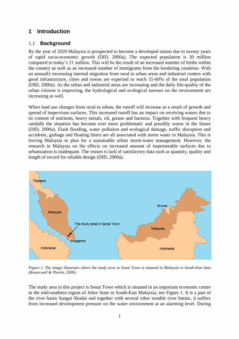
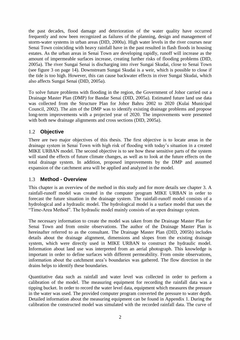
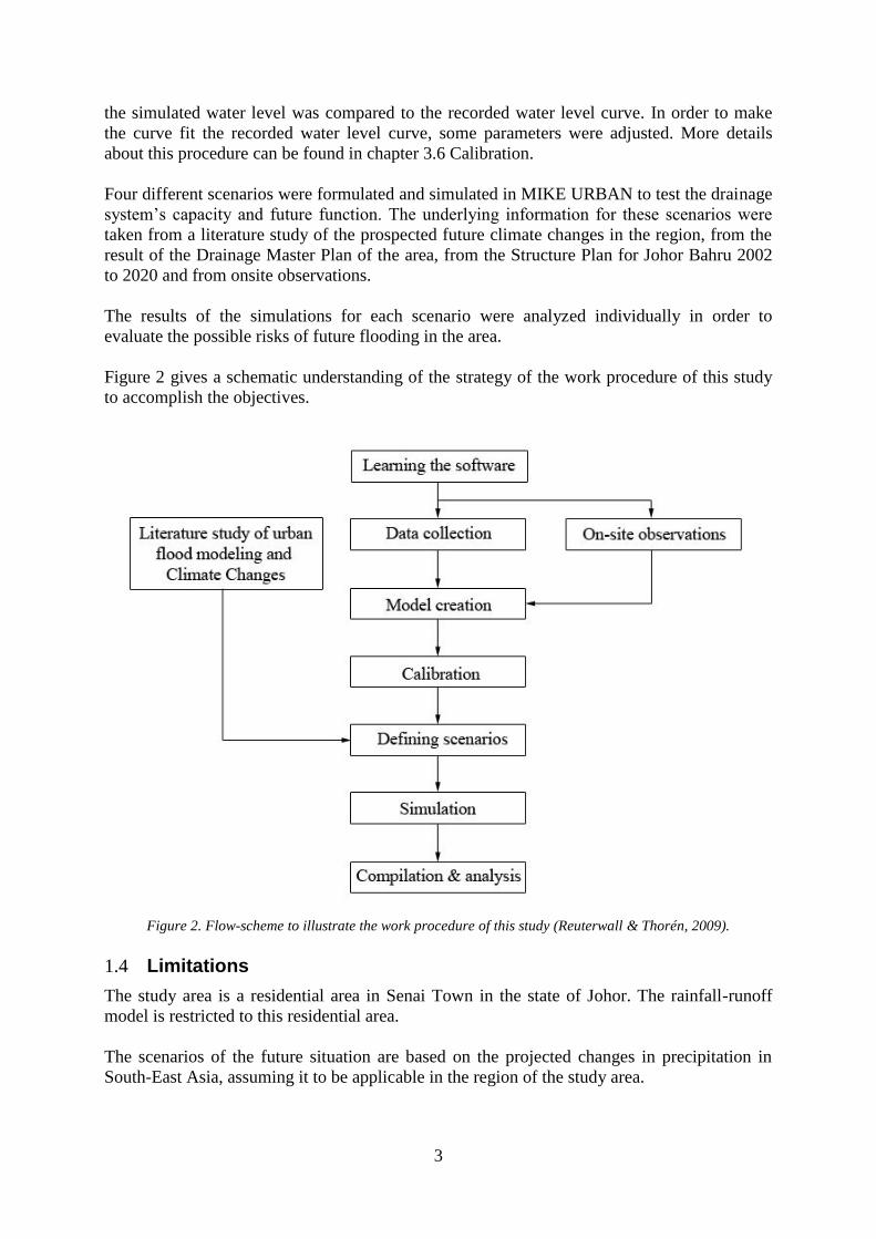
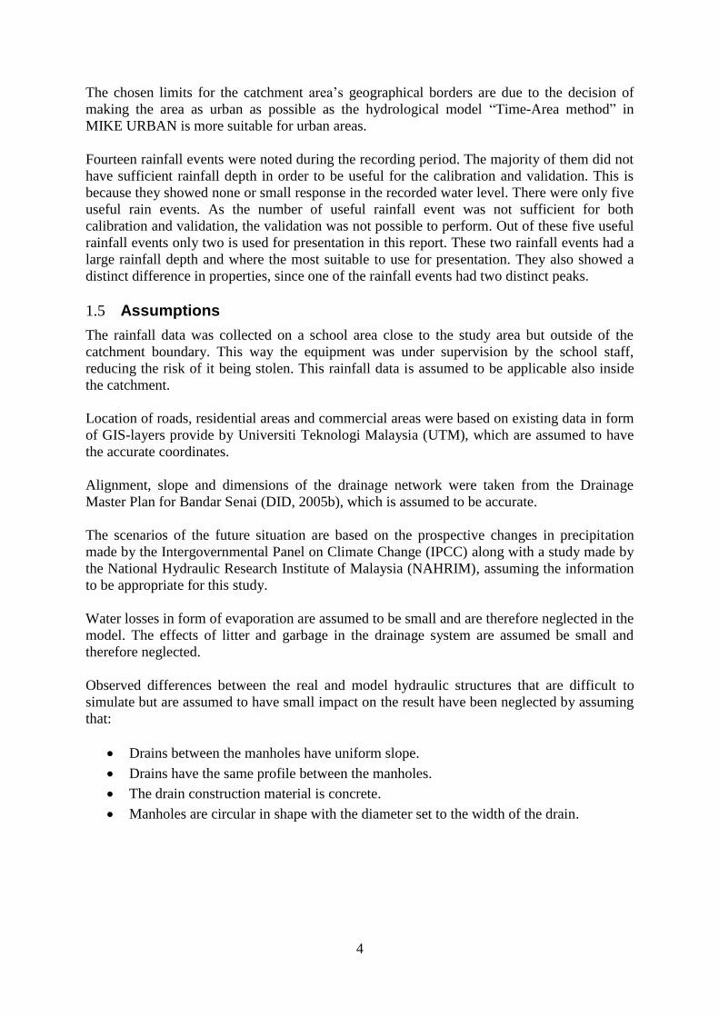
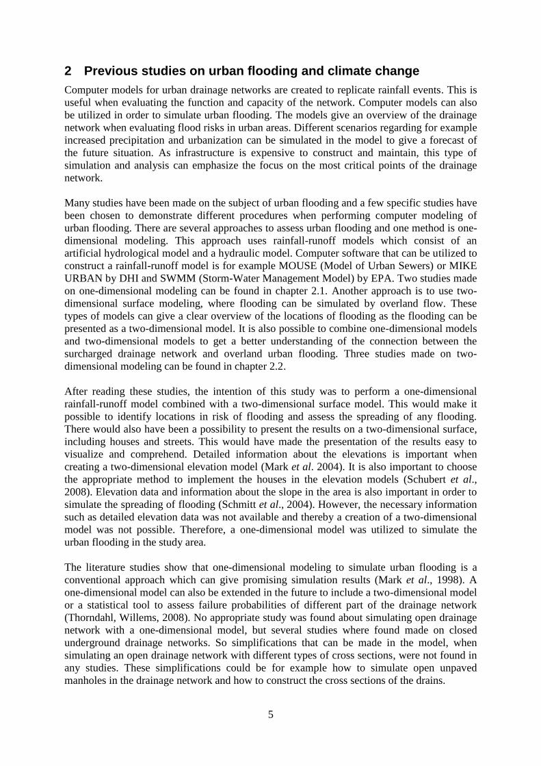


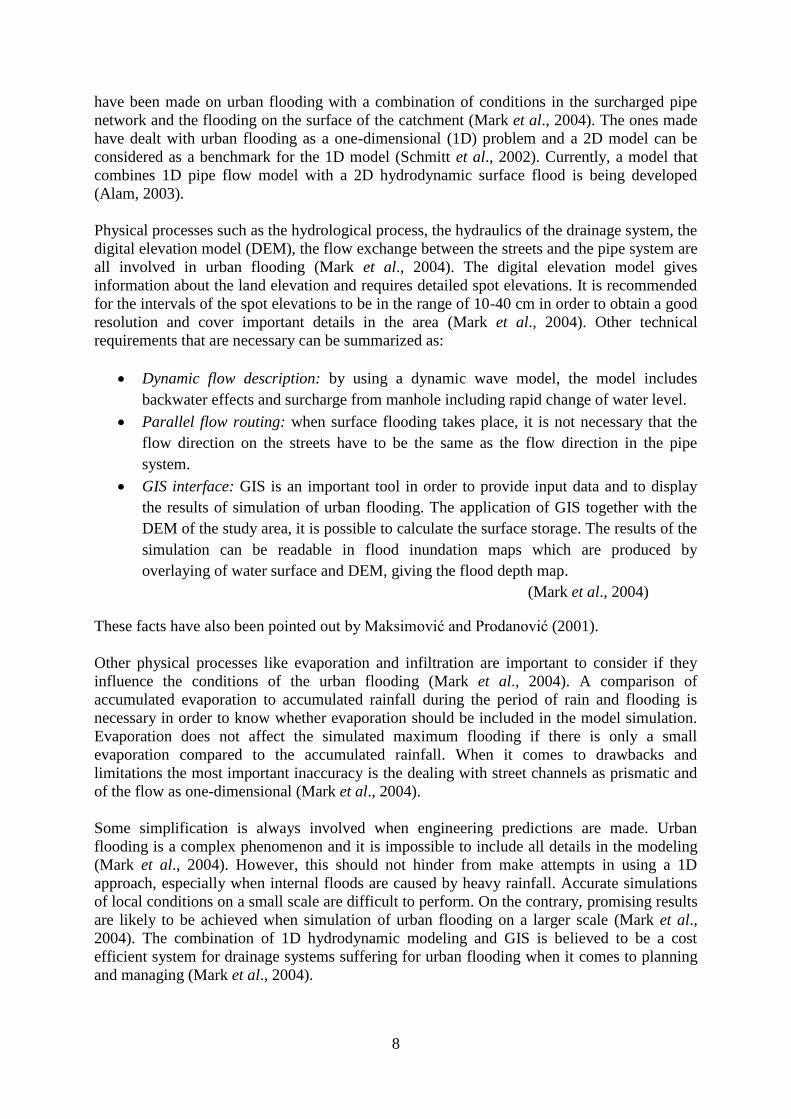
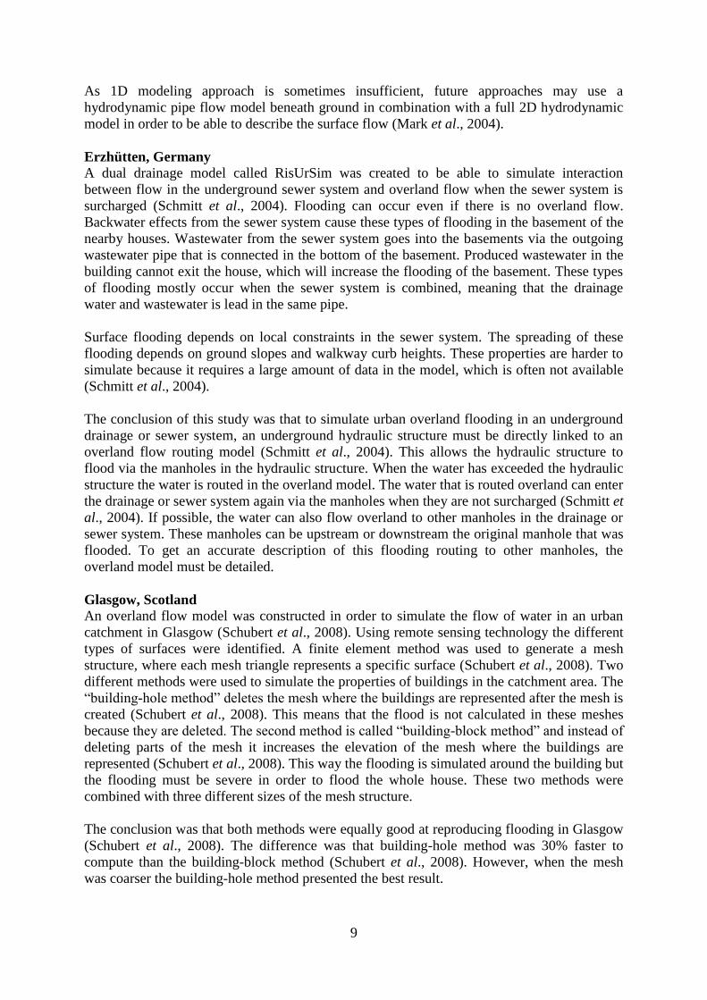

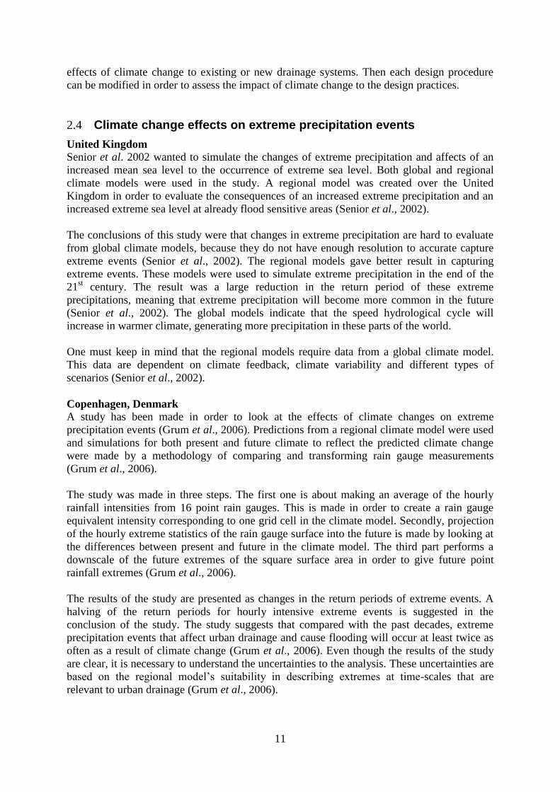

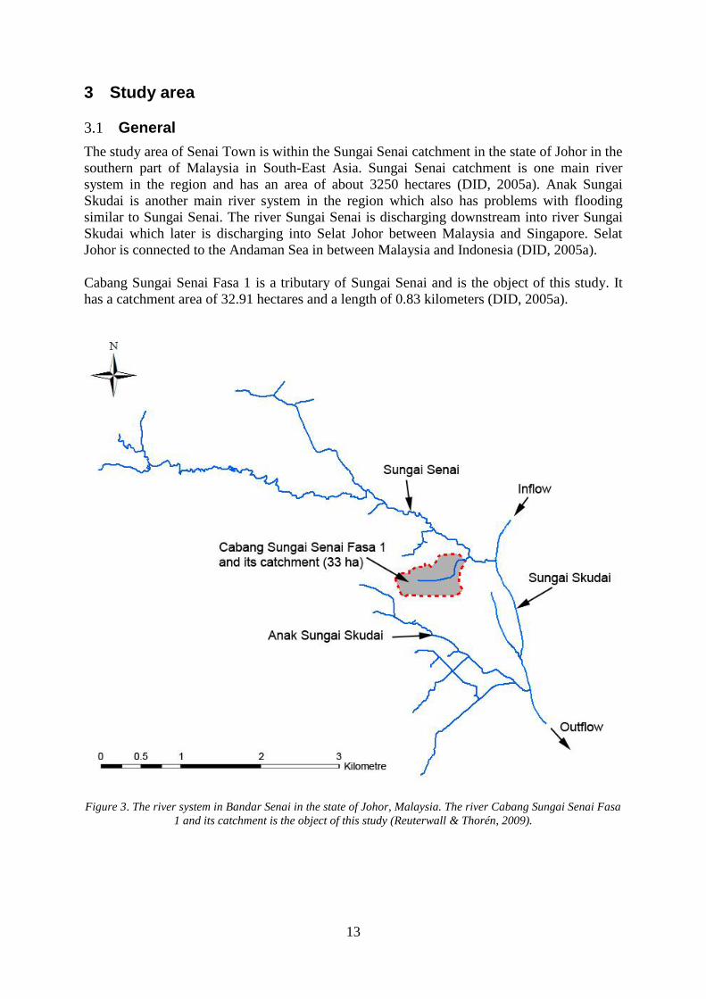

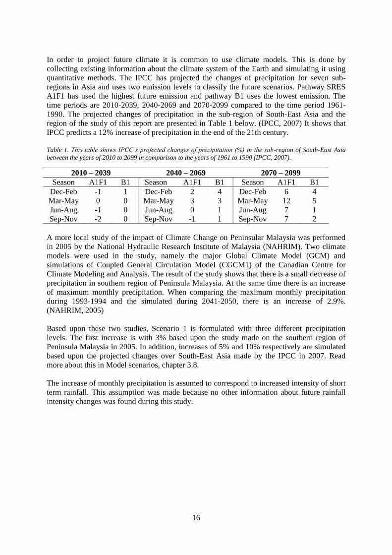
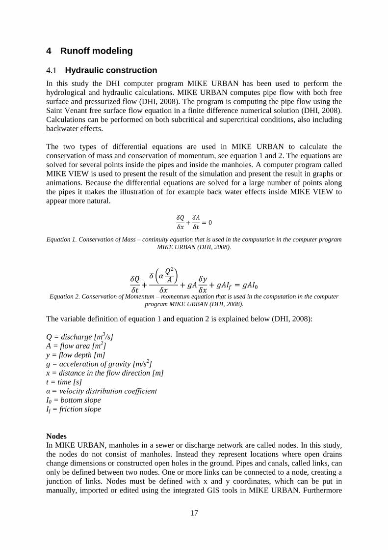
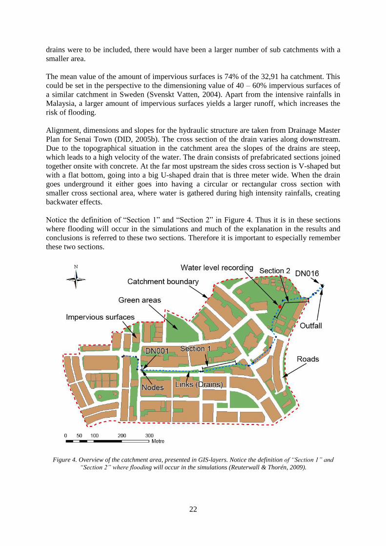
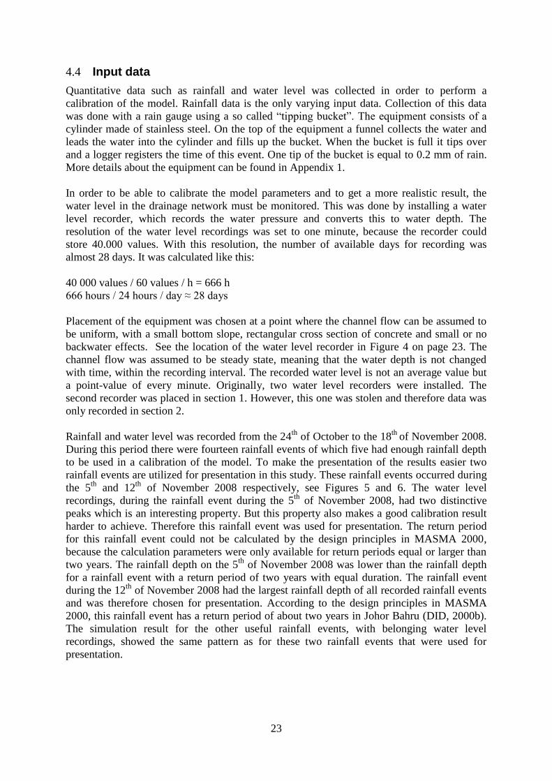
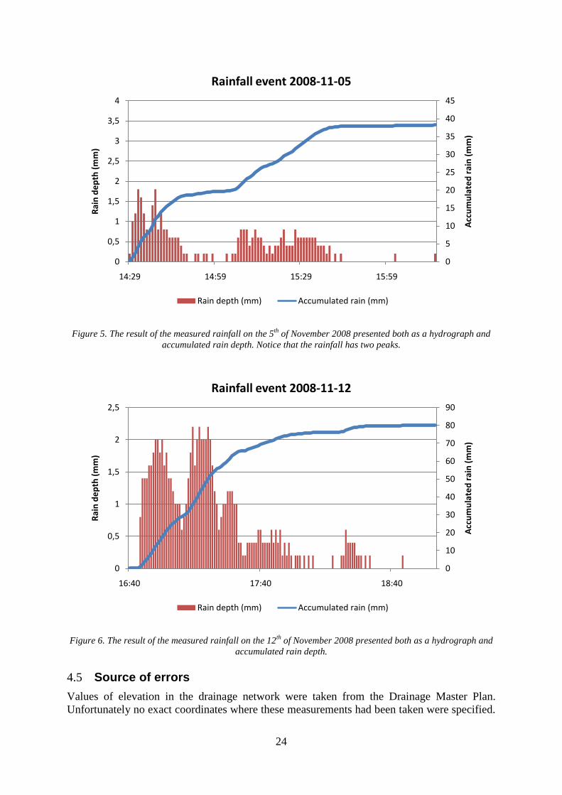
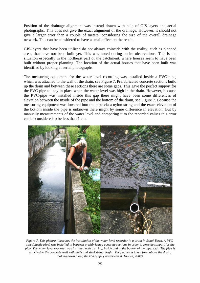

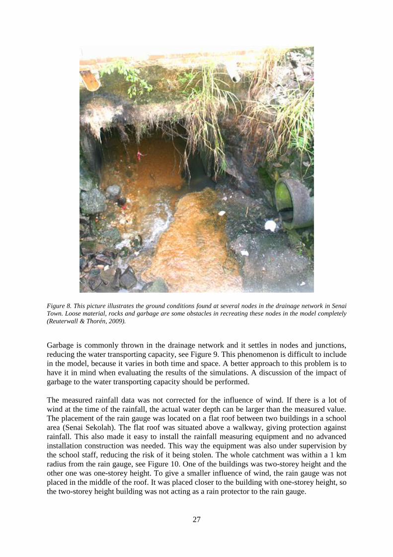
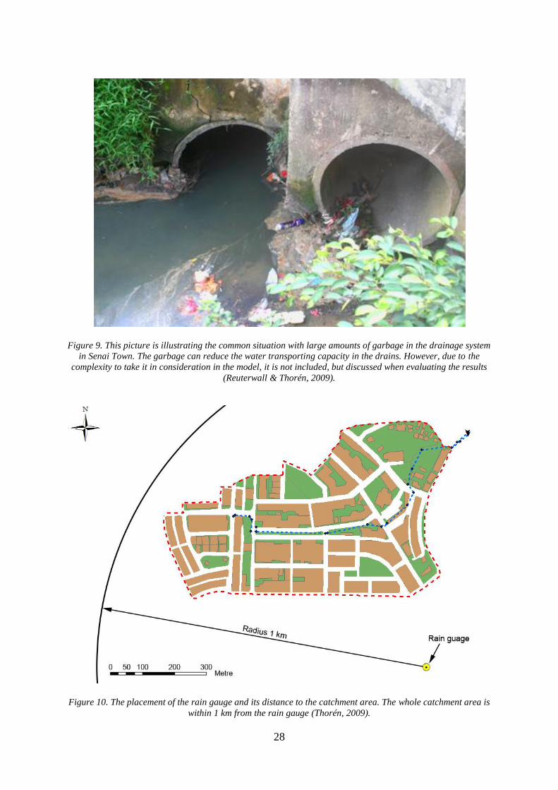
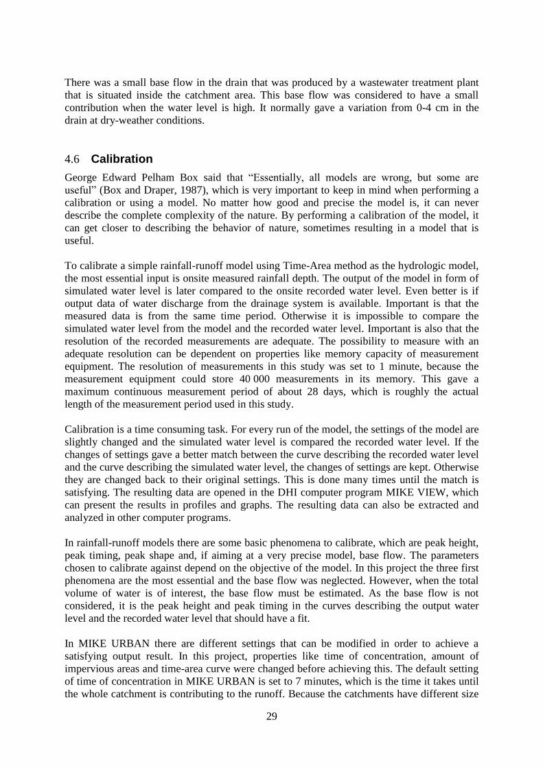
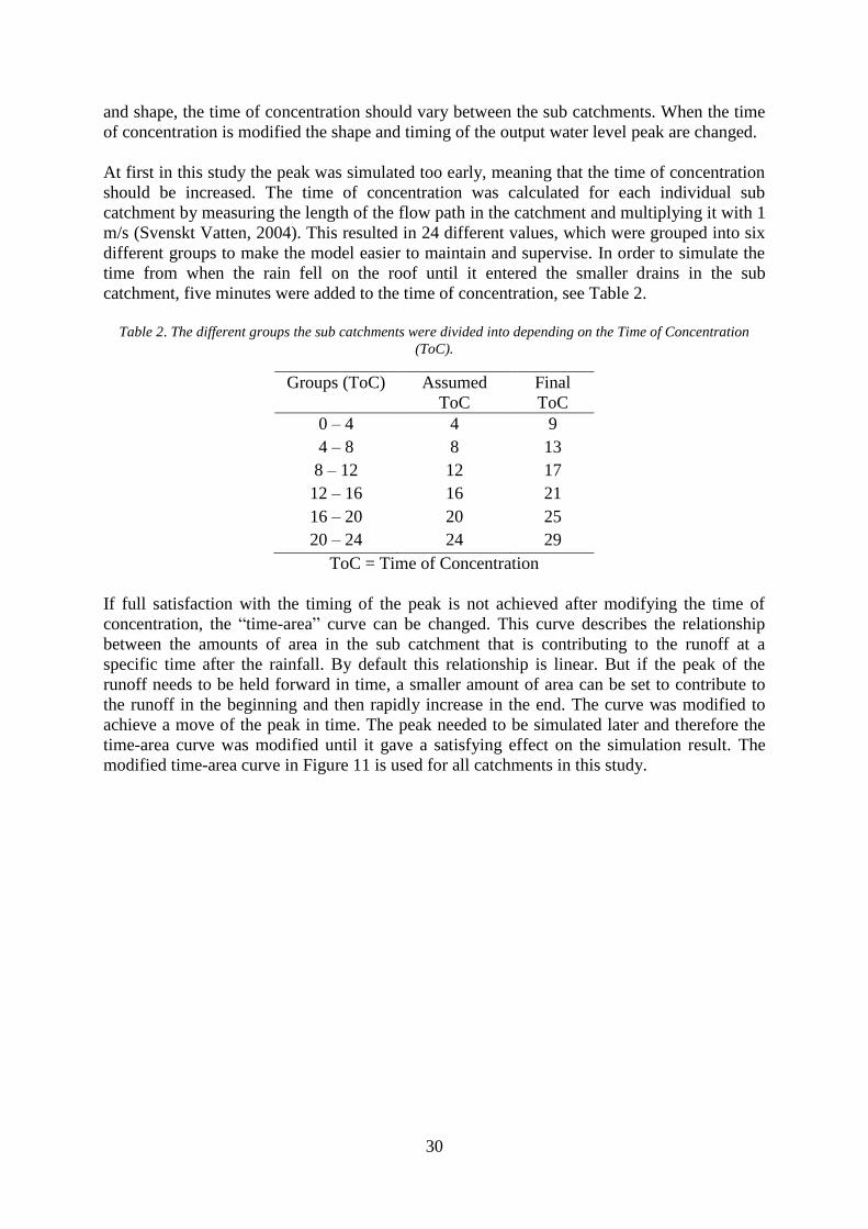
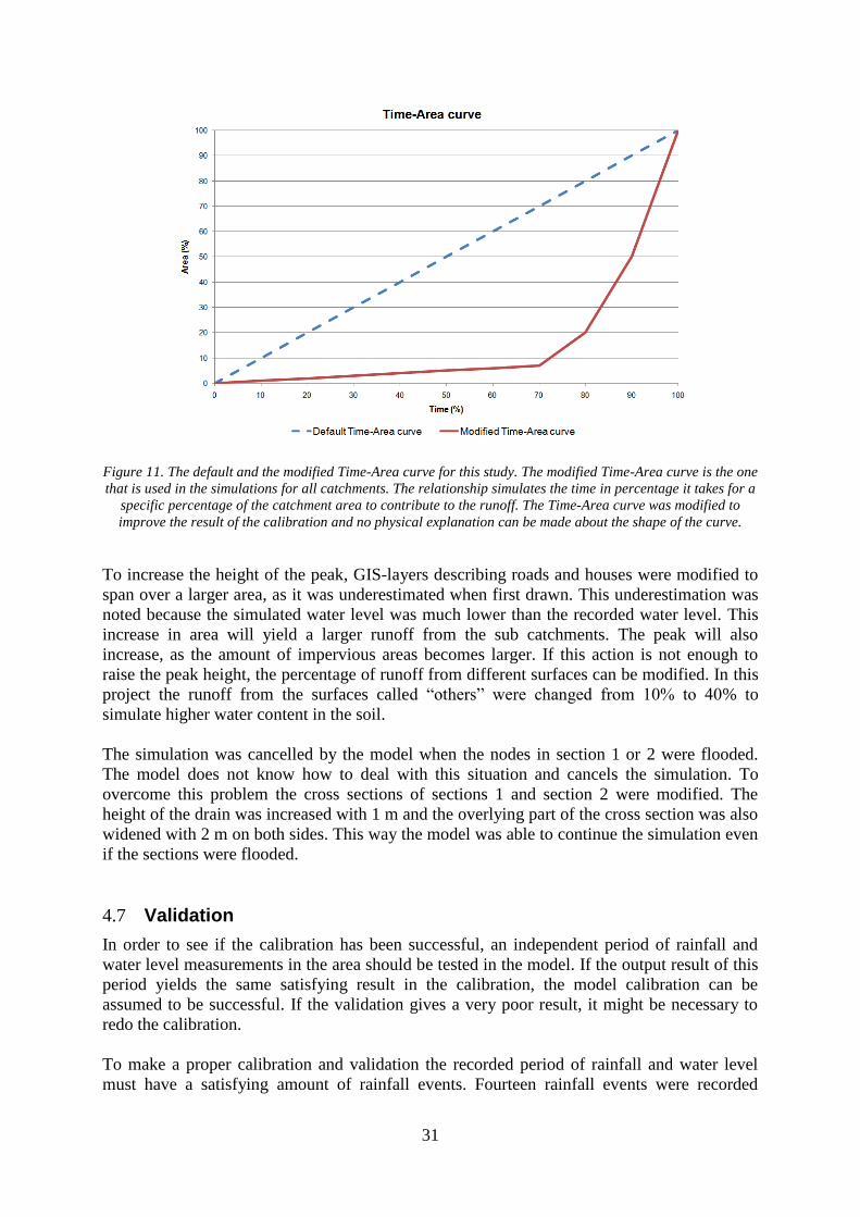

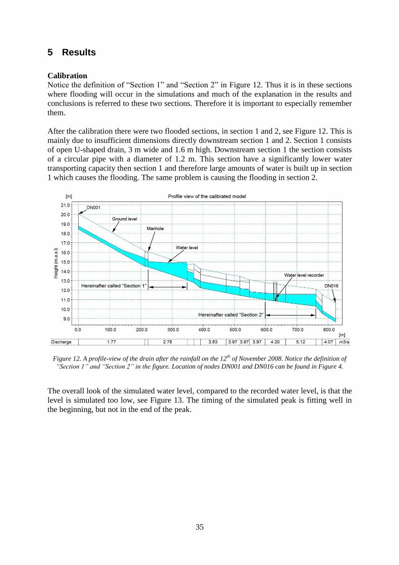
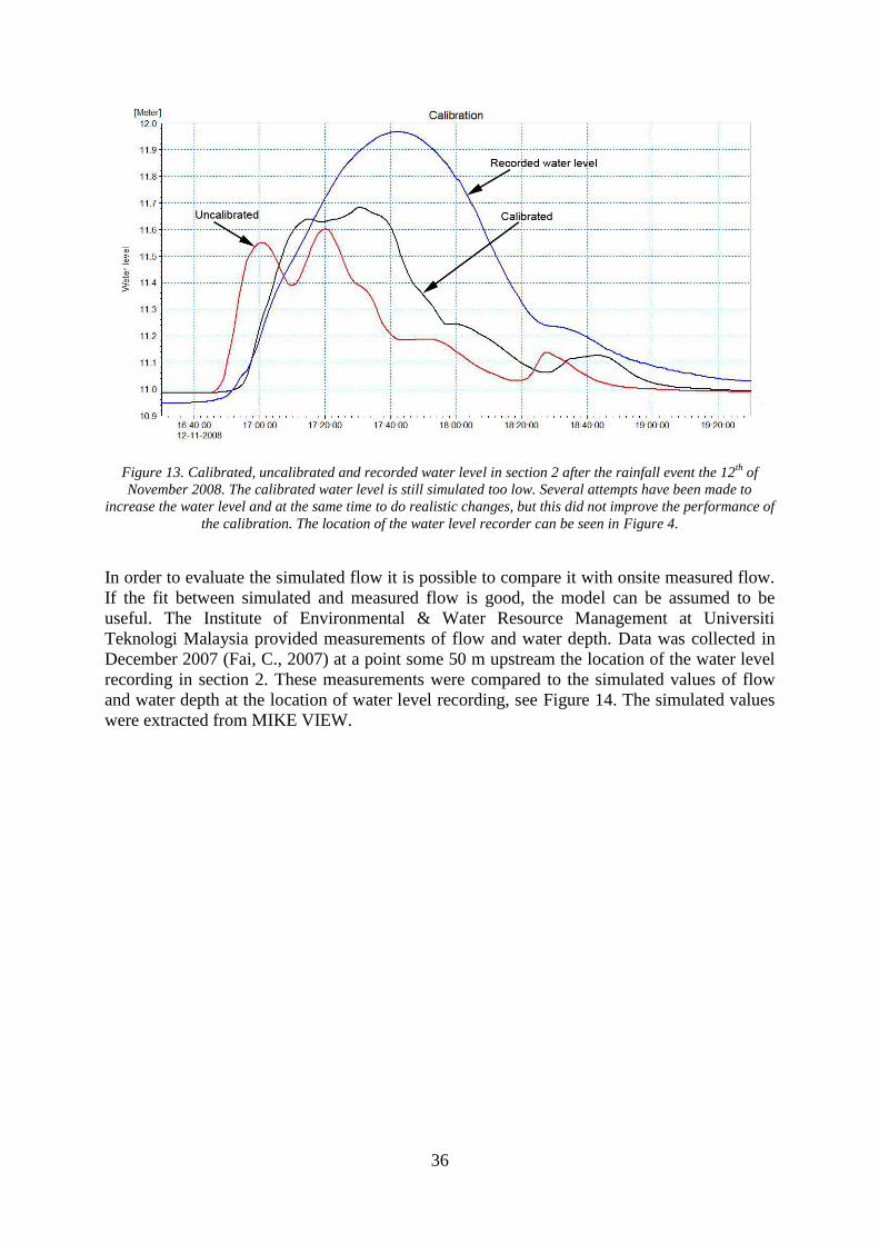
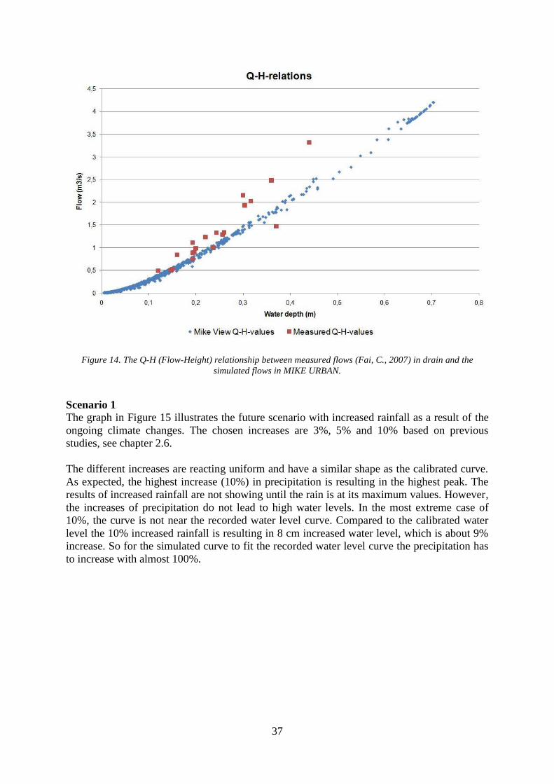
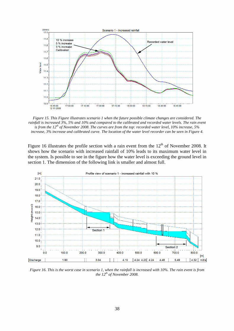
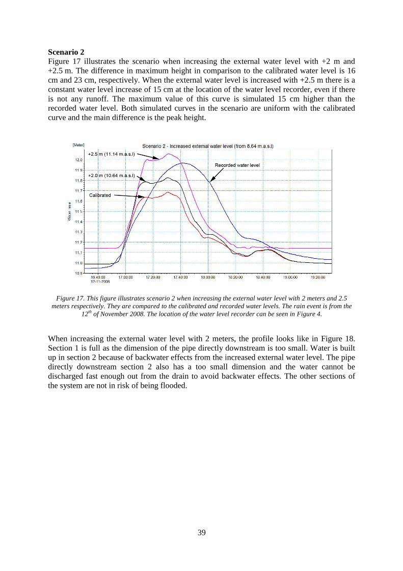
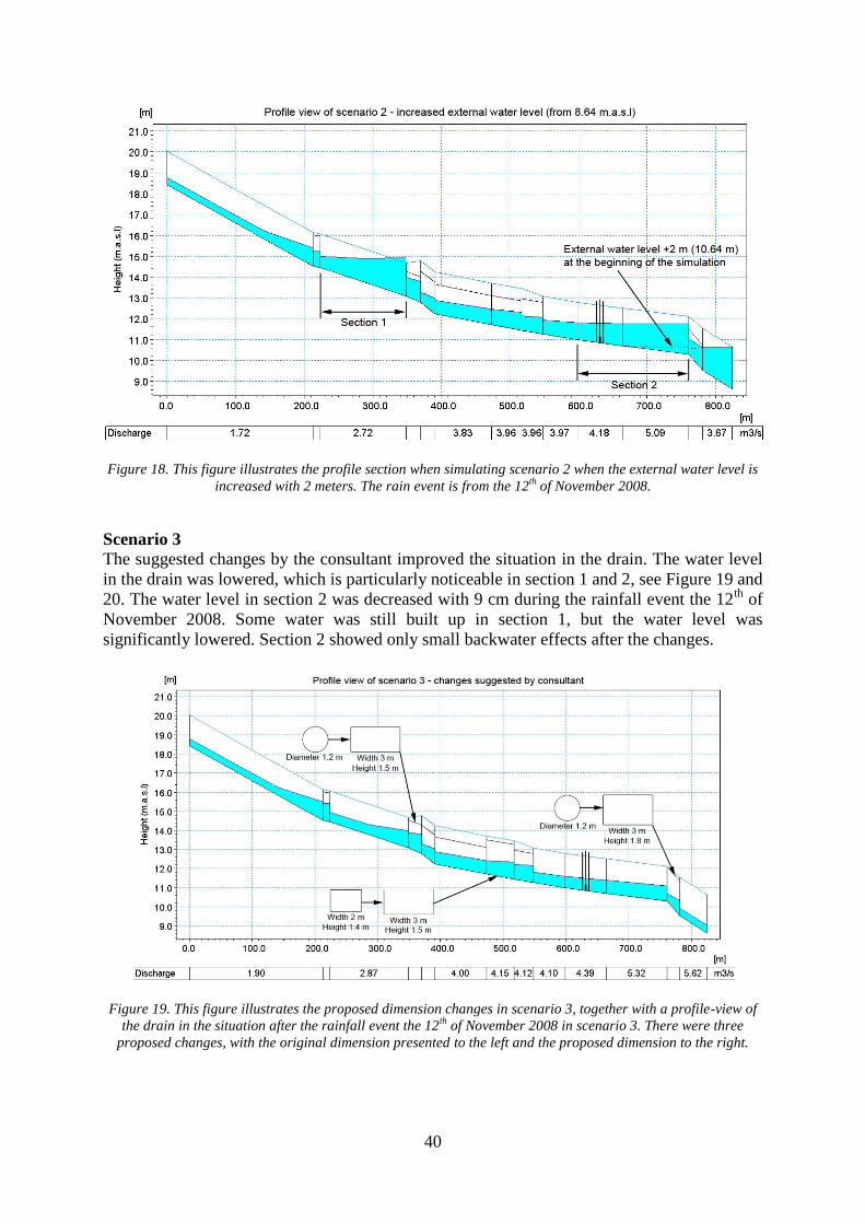
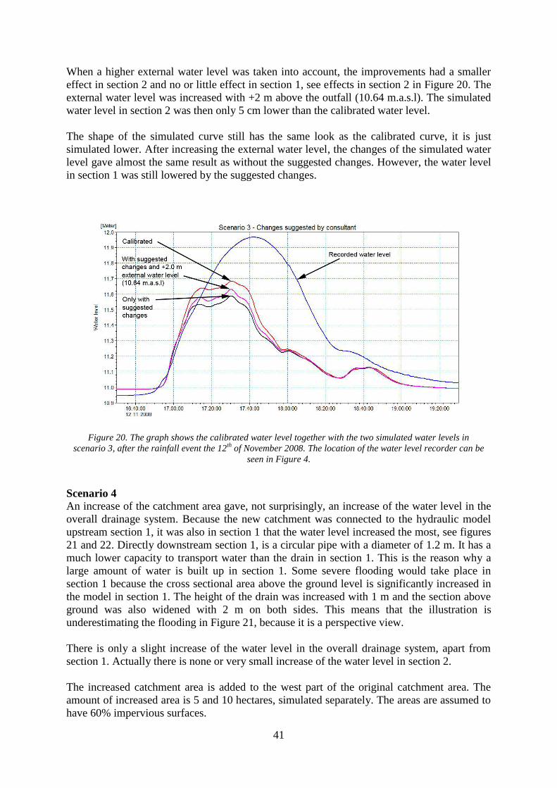
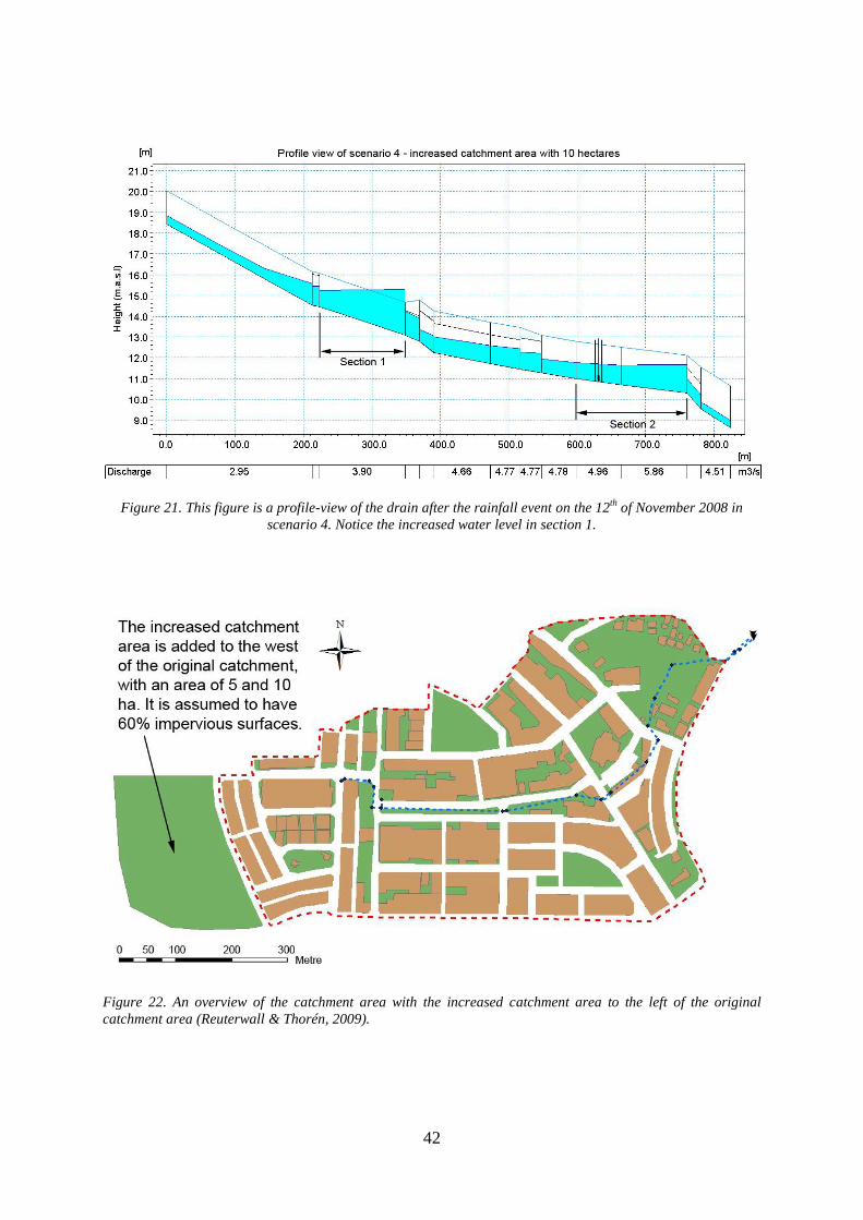
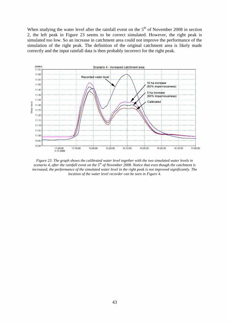

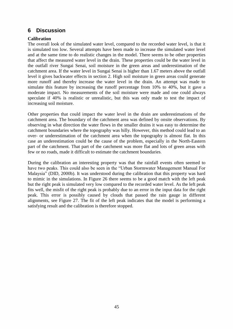
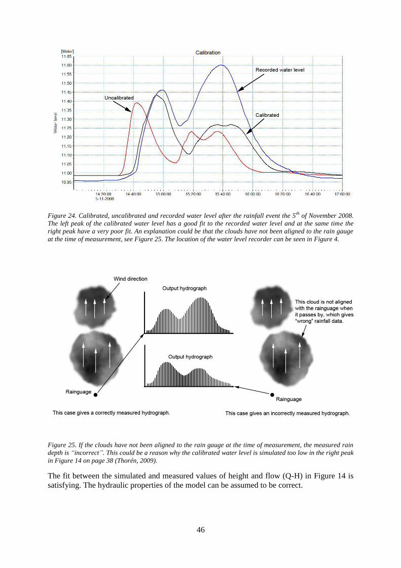


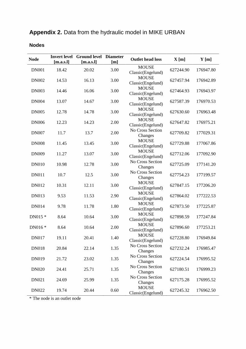
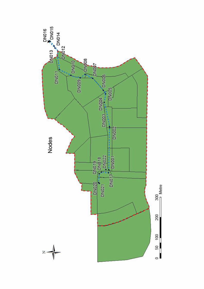
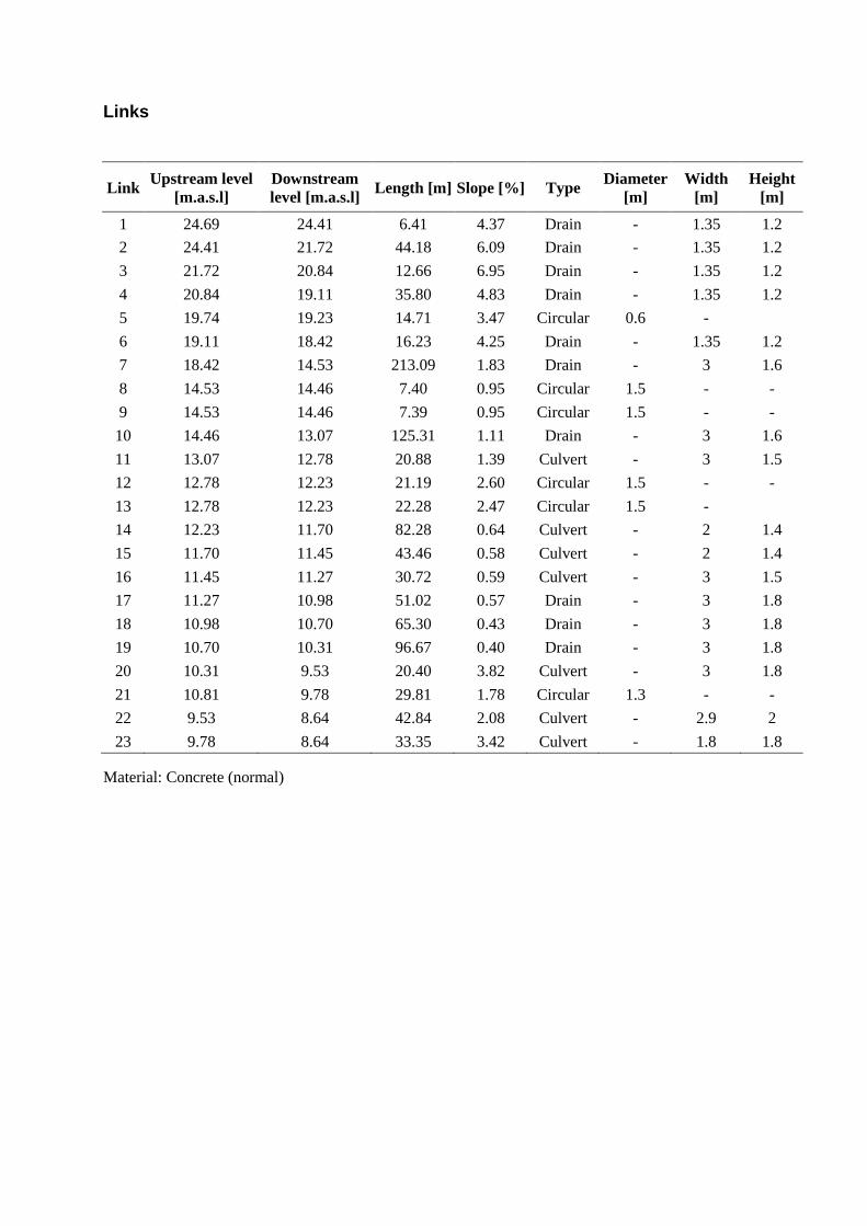
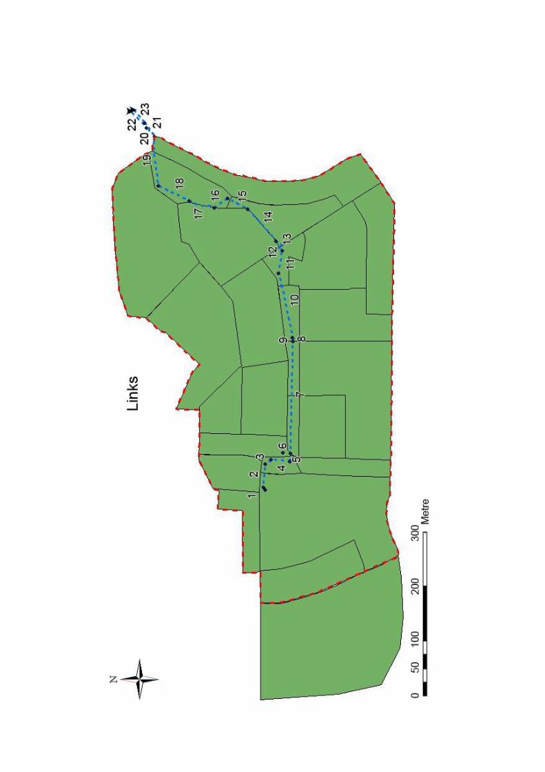
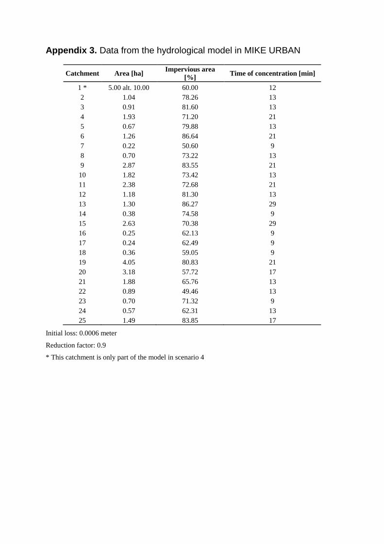
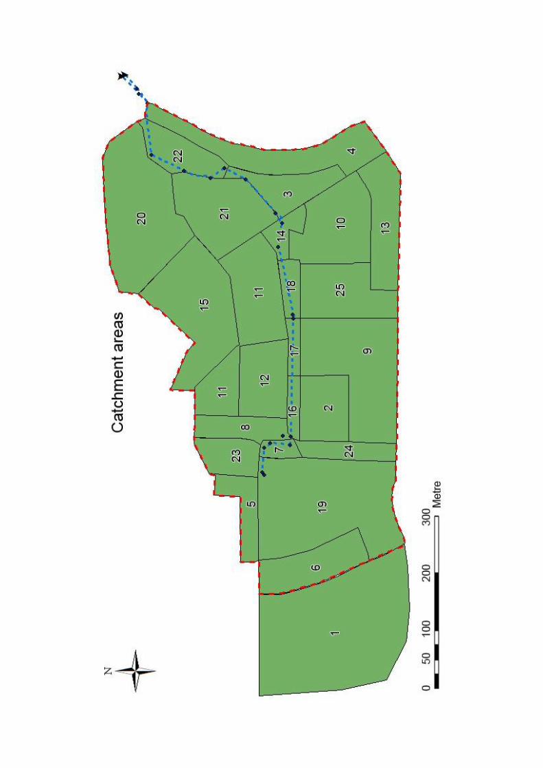
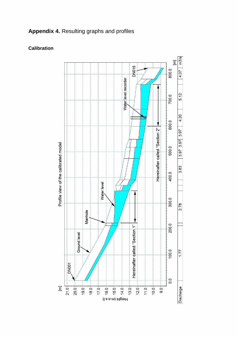
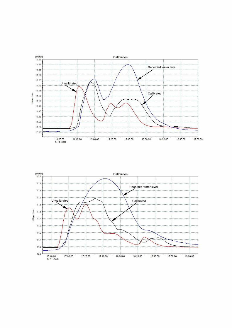
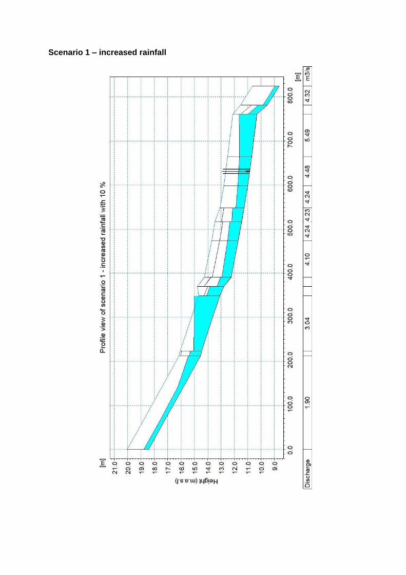
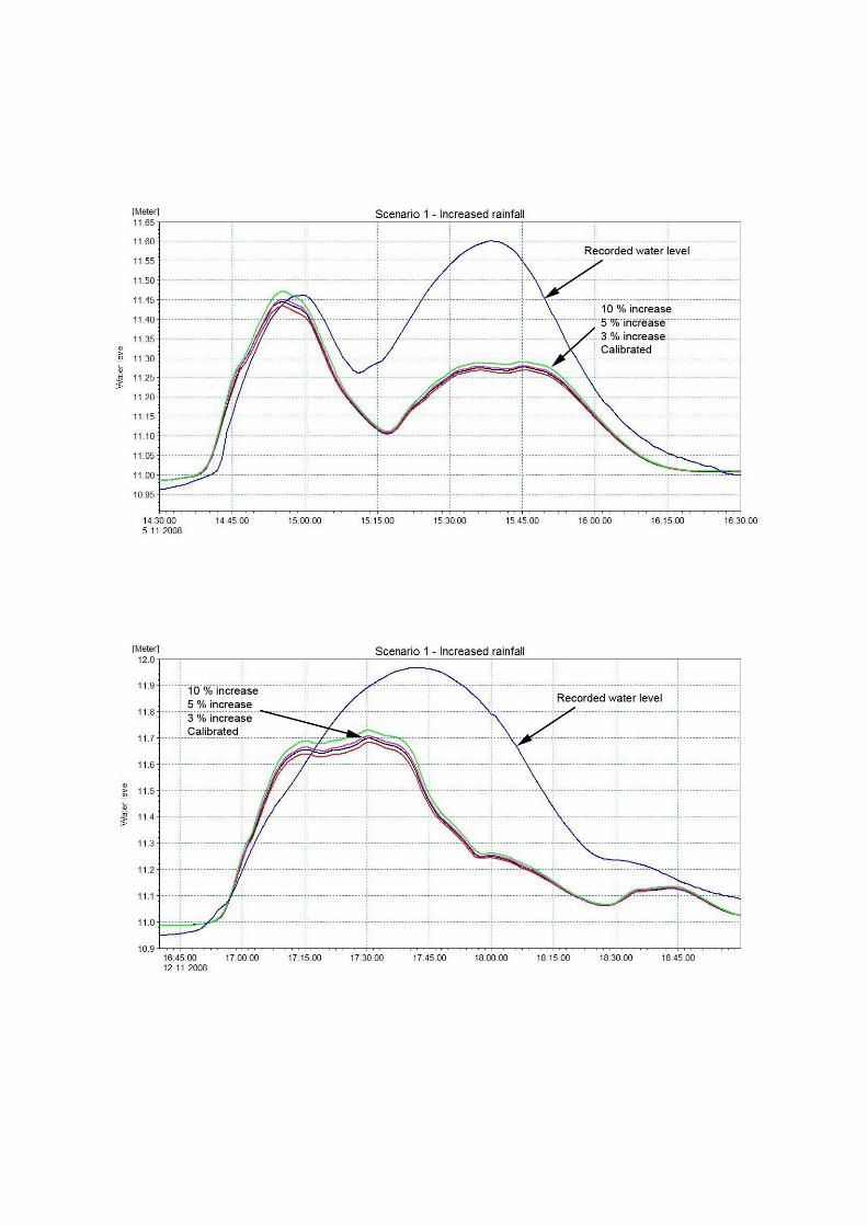
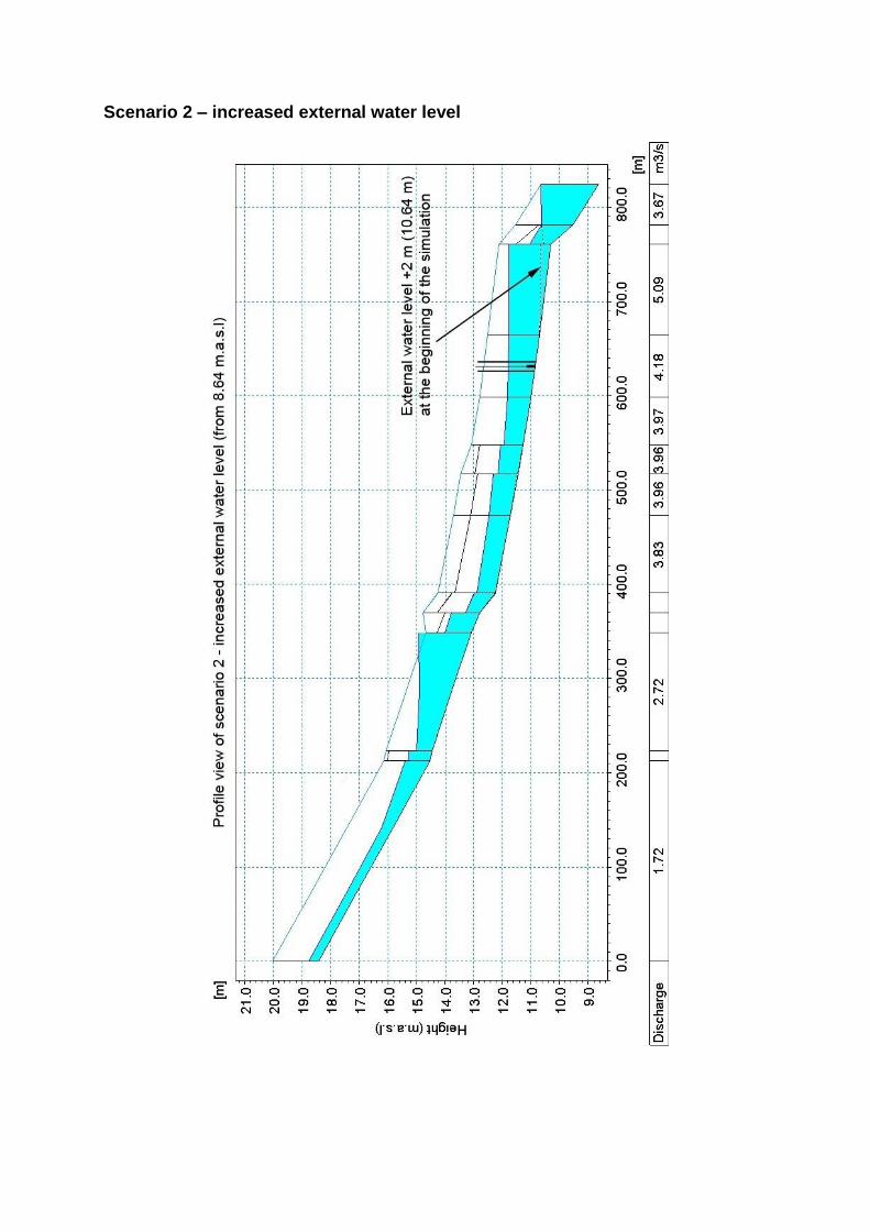
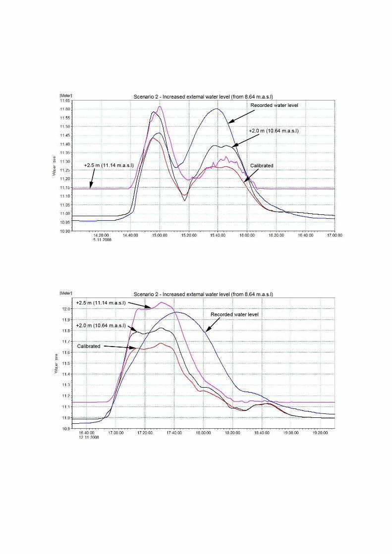
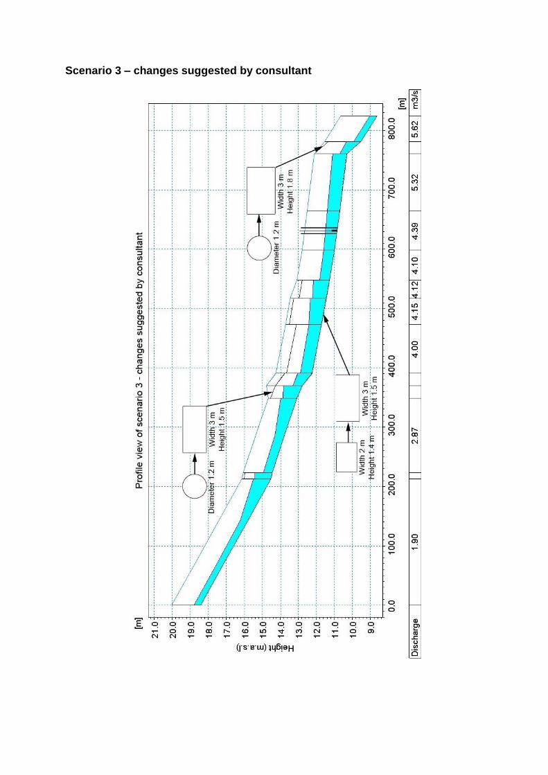
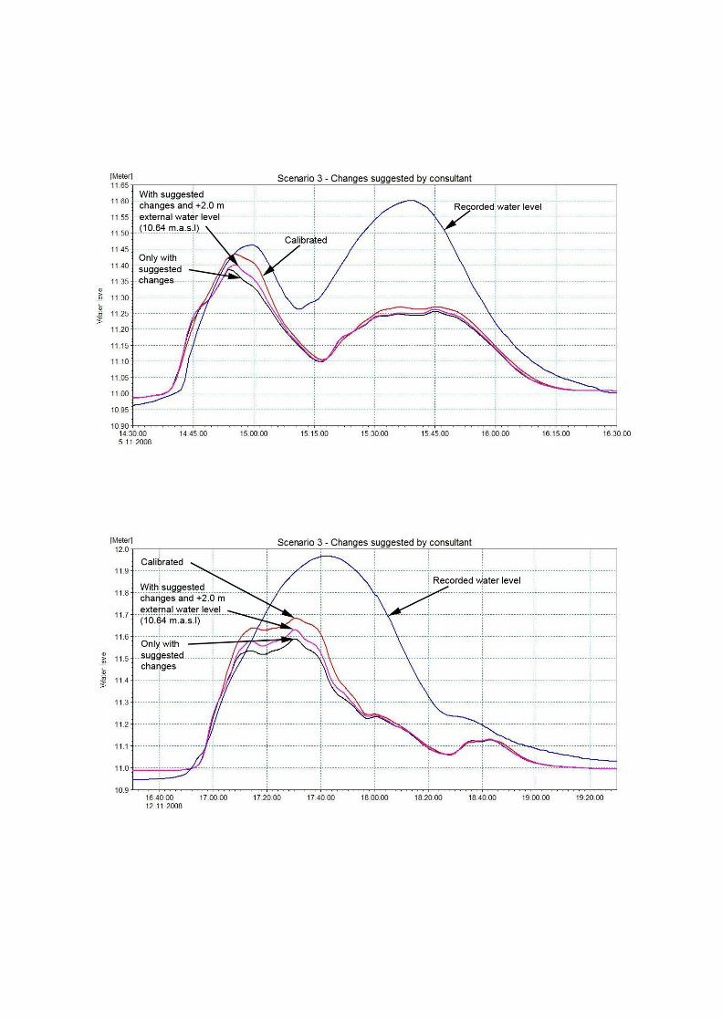
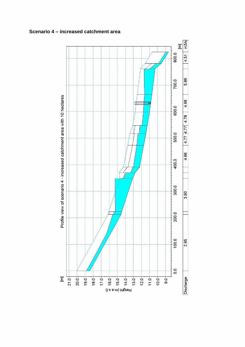
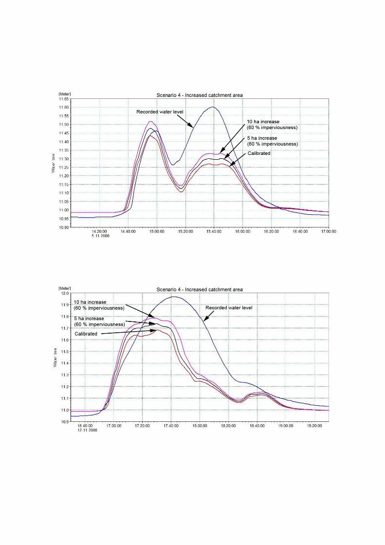

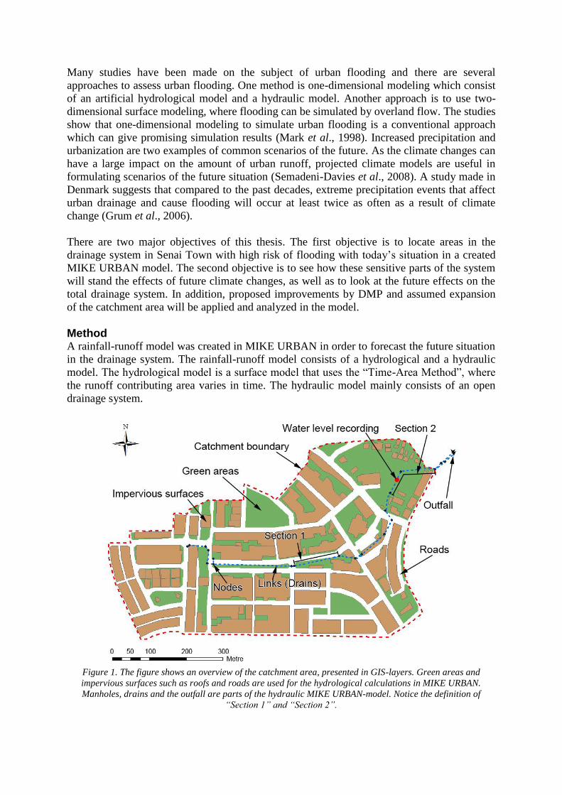
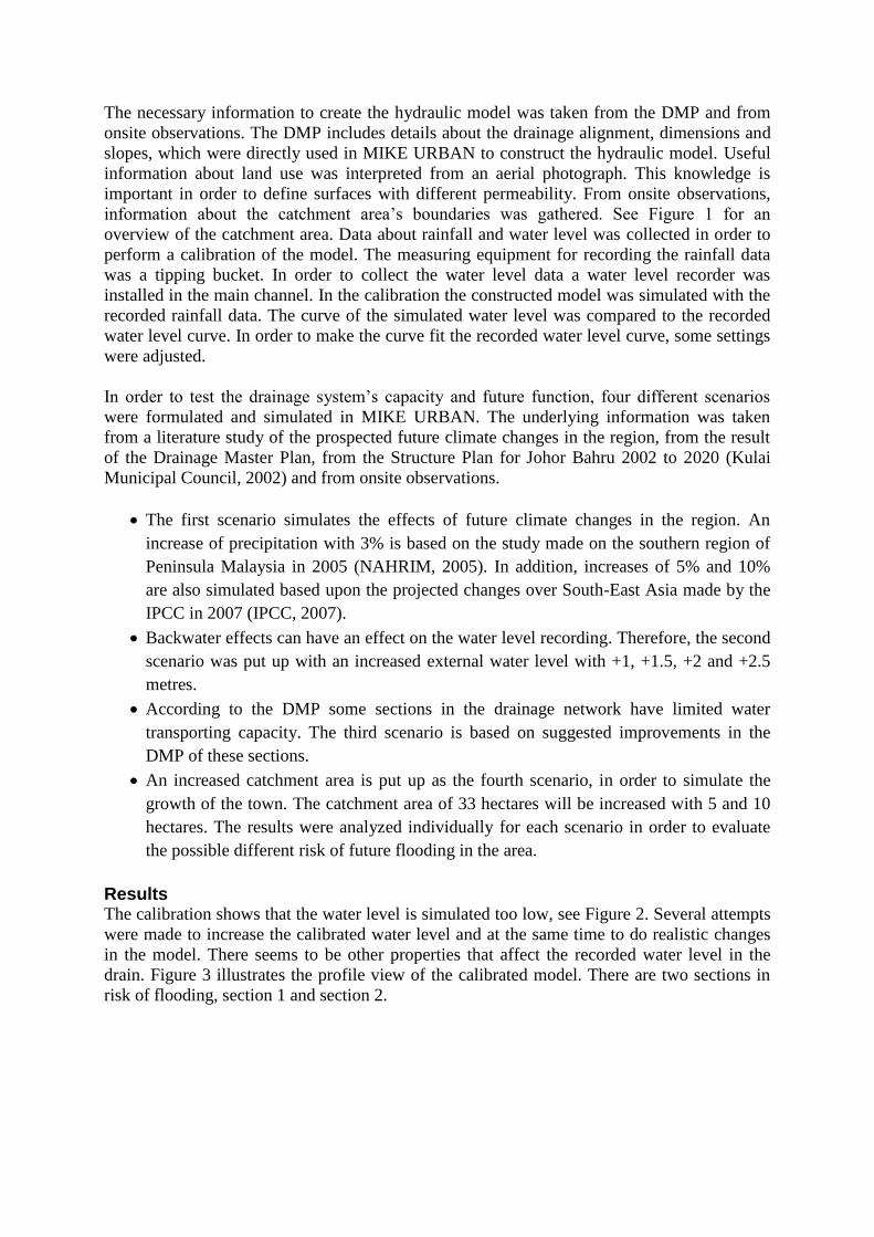
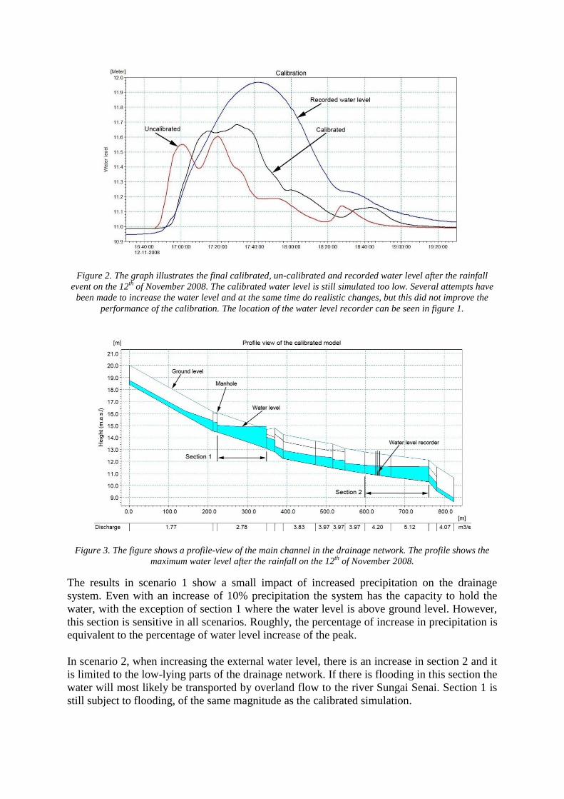
![Geological Map of Mongolia [L-47-IX] · 98 45'o 99 00'o 47o 10' 47o 20' 47 o 00' 46 o 50' 46 o 40' 98 00' 98 15' o98 30' 98 00' 98 15'o 98 30' 98 45'o 99 00' 47 10' 47 47 o 46 o 50'](https://static.documents.pub/doc/80x56/5f6287549cbf13303b1c6c4a/geological-map-of-mongolia-l-47-ix-98-45o-99-00o-47o-10-47o-20-47-o-00-46.jpg)


