Open AcceResearch articleIdentification of gene expression patterns using planned linear contrastsHao Li*1, Constance L Wood1, Yushu Liu1, Thomas V Getchell2,4, Marilyn L Getchell3,4 and Arnold J Stromberg1
Address: 1Department of Statistics, University of Kentucky, 817 Patterson Office Tower, Lexington, KY40536-0027, USA, 2Department of Physiology, College of Medicine, Lexington, KY40536-0298, USA, 3Department of Anatomy and Neurobiology, College of Medicine, Lexington, KY40536-0298, USA and 4309 Sanders-Brown Center on Aging, University of Kentucky Medical Center, Lexington, KY40536-0230, USA
AbstractBackground: In gene networks, the timing of significant changes in the expression level of eachgene may be the most critical information in time course expression profiles. With the same timingof the initial change, genes which share similar patterns of expression for any number of samplingintervals from the beginning should be considered co-expressed at certain level(s) in the genenetworks. In addition, multiple testing problems are complicated in experiments with multi-leveltreatments when thousands of genes are involved.
Results: To address these issues, we first performed an ANOVA F test to identify significantlyregulated genes. The Benjamini and Hochberg (BH) procedure of controlling false discovery rate(FDR) at 5% was applied to the P values of the F test. We then categorized the genes with asignificant F test into 4 classes based on the timing of their initial responses by sequentially testinga complete set of orthogonal contrasts, the reverse Helmert series. For genes within each class,specific sequences of contrasts were performed to characterize their general 'fluctuation' shapesof expression along the subsequent sampling time points. To be consistent with the BH procedure,each contrast was examined using a stepwise Studentized Maximum Modulus test to control thegene based maximum family-wise error rate (MFWER) at the level of αnew determined by the BHprocedure. We demonstrated our method on the analysis of microarray data from murineolfactory sensory epithelia at five different time points after target ablation.
Conclusion: In this manuscript, we used planned linear contrasts to analyze time-coursemicroarray experiments. This analysis allowed us to characterize gene expression patterns basedon the temporal order in the data, the timing of a gene's initial response, and the general shapes ofgene expression patterns along the subsequent sampling time points. Our method is particularlysuitable for analysis of microarray experiments in which it is often difficult to take sufficientlyfrequent measurements and/or the sampling intervals are non-uniform.
BackgroundRecent advances in DNA microarray technologies havemade it possible to investigate the transcriptional portionof gene networks in a variety of organisms. When micro-array experiments are performed to monitor gene expres-sion over time, researchers can address questionsconcerning the detection of the cellular processes underly-ing the observed regulatory effects, inference of regulatorynetworks and, ultimately, assignment of functions to thegenes analyzed in the time courses.
There is a natural connection between gene function andgene expression. Based on our understanding of cellularprocesses, genes that are contained in a particular path-way, or respond to a common internal or external stimu-lus, should be co-regulated and consequently, shouldshow similar patterns of expression. Therefore, identifyingpatterns of gene expression and grouping genes intoexpression classes may provide much greater insight intotheir biological functions. A large group of statisticalmethods, generally referred to as "cluster analysis", havebeen developed to identify genes that behave similarlyacross a range of experimental conditions, including timecourses. These statistical algorithms can be divided intotwo classes, depending on whether they are based on 'sim-ilarity' measures or not. Methods based on 'similarity'measures rely on defining a distance (or 'dissimilarity')between gene expression vectors; Euclidean distance and/or the Pearson correlation coefficient are the two mostcommonly used distance measures. Examples of similar-ity measures-based methods are hierarchical clustering[1], k-means [2], self-organization maps (SOM) [3,4], andsupport vector machine (SVM) [5]. These methods do notconsider the temporal structure of the data when used toanalyze time-course experiments. In addition, somemethods could confuse the clusters because the actualexpression patterns of the genes themselves become lessrelevant as clusters grow in size [6].
The clustering methods in the second class are based onstatistical models, without defining a 'similarity' measure.Using statistical models to represent clusters changes thequestion from how close two data points are to how likelya given data point is under the model. Such clusteringmethods are more commonly used to analyze time-coursemicroarray experiments. Examples of such methods arebased on cubic spline [7], ANOVA model [8], autoregres-sive curves [9], first-order kinetics [10], Hidden MarkovModels [11,12], Bayesian model average [13], order-restricted inference methodology [14], and Gaussian Mix-ture Models [15-19]. Such approaches may be restrictedeither by the rigorous assumptions of the stochastic mod-els [9,11,12], or by the small number of time points andnon-uniform sampling intervals in gene expression data[7,9,10].
In gene networks, the level of expression of individualgenes changes based on their functional position in thenetwork. Therefore, the most critical information in timecourse expression profiles is the timing of the changes inexpression level for each gene [10], and secondarily is thegeneral shape of its expression pattern [20,21]. In addi-tion, different genes will be activated or inactivated ateach level of a gene network. Therefore it may not be rea-sonable to expect that the expression levels of those co-expressed genes will go up and down concordantly all theway through the entire sampling period. With the sametiming of initial change, genes which share similar patternof expression for any number of sampling intervals fromthe beginning should be considered co-expressed at cer-tain level(s) in the gene network. However, statisticalmethods to analyze these patterns have not yet beenreported.
Attention to the multiplicity problem in gene expressionanalysis has been increasing. Numerous methods areavailable for controlling the family-wise type I error rate(FWER). Since microarray experiments are frequentlyexploratory in nature and the sample sizes are usuallysmall, Benjamini and Hochberg [22] suggested a poten-tially more powerful procedure, the false discovery rate(FDR), to control the expected proportion of errorsamong the identified differentially expressed genes. Anumber of studies for controlling FDR have followed [23-29]. In microarray experiments with multi-level treat-ments, the multiple testing problems are two dimen-sional. Not only are thousands of genes involved, but foreach gene, either pre-selected contrasts or post-hoc com-parisons may be needed to characterize its expression pat-tern. There are very few studies that have investigated howto deal with such multiple-testing problems in the micro-array literature [30].
In this manuscript, we propose a different strategy basedon planned linear contrasts (pre-selected contrasts) forthe analysis of time-course microarray experiments. Spe-cifically, our approach takes into consideration the tem-poral order in the data, including the timing of a gene'sinitial response and the general shapes of gene expressionpatterns along the subsequent sampling time points. Ourmethods are particularly suitable for analysis of microar-ray experiments in which it is often difficult to take suffi-ciently frequent measurements and/or the samplingintervals are non-uniform. We demonstrated our methodon the analysis of microarray data from murine olfactorysensory epithelia at five different time points after targetablation.
ResultsOlfactory sensory neurons (OSNs) detect odors in theambient environment and transmit the sensory informa-
Page 2 of 11(page number not for citation purposes)
tion directly to the brain. The death of OSNs can beinduced experimentally by microsurgical removal of theiraxonal targets in the brain (olfactory bulbectomy, OBX).The temporal regulation of genes associated with thedeath of OSNs and other cellular processes as a result ofOBX can be systematically investigated at 2 hr, 8 hr, 16 hrand 48 hr post-OBX. Based on the statistical methodsdescribed (see Methods), 1234 genes were considered tobe significant by the procedure of controlling FDR at 5%
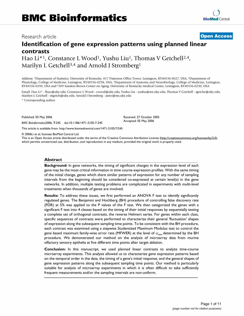
for multiple testing across genes. The largest P-value con-sidered to be significant was 0.009545 as determined bythe FDR procedure. The temporal regulation of these 1234genes fell into four distinct classes based on the first signif-icant change in their temporal profile that occurred ateither 2 hr (Class I), 8 hr (Class II), 16 hr (Class III), or 48hr (Class IV) post-OBX. Among the 1234 genes (Figure 1),212 were grouped into Class I in which the differentialexpression of these genes was detected as early as 2 hours
Flow chart illustrating the statistical procedure to classify gene expression patternsFigure 1Flow chart illustrating the statistical procedure to classify gene expression patterns. A 1 × 5 ANOVA F test was performed for each of the 6464 genes after data filtering. By controlling FDR at 5%, 1234 genes were selected, 1105 of which were clustered into 4 classes based on the timing of their initial significant change in expression level. The fluctuation patterns of genes in each class were examined using planned linear contrasts.
6464 Present Probe Sets on MG_U74Av2
Control FDR at 5%
1234 genes left
1105 genes classified based on initial response 129 genes with marginal changes
1X5 ANOVA F
212 genes
23 patterns
76 genes
10 patterns
292 genes
6 patterns
525 genes
2 patterns
Class I Class II Class III Class IV
Preplanned contrasts
Table 1: Example of genes from different classesThree genes from each of the 4 classes were selected to illustrate their expression patterns. P_F: P values for the overall F test; P_t: P values at their initial responses; FC: fold changes at their initial responses, where a negative sign indicates down-regulation.
Class Gene P_F P_t FC Gene Function
I Pdcd5 5.40E-03 6.30E-04 1.2 apoptosisCetn3 7.40E-05 3.10E-04 1.2 Ca binding
after target ablation. Seventy-six genes were grouped intoClass II, 292 genes whose expression level first changed at16 hr post-OBX into Class III, and 525 genes whoseexpression level first changed at 48 hours after the surgerywere grouped into Class IV. The remaining 129 genes didnot pass our selection criteria although their ANOVA Ftests were significant.
The expression level of the gene for olfactory marker pro-tein Omp, which is expressed in mature OSNs, wasunchanged at 2 hr and 8 hr following OBX. The initialchange, a down-regulation at 16 hr post-OBX, indicatedthat degeneration was evident between 8 hr and 16 hrpost-OBX (Figure 2). The significant down-regulation ofOmp (p = 1.6E-5, Table 1) continued to the 48 hr time-point that was accompanied by a -1.6 FC in OMP mRNA,indicating degenerative changes in OSNs accompanyingtheir cell death.
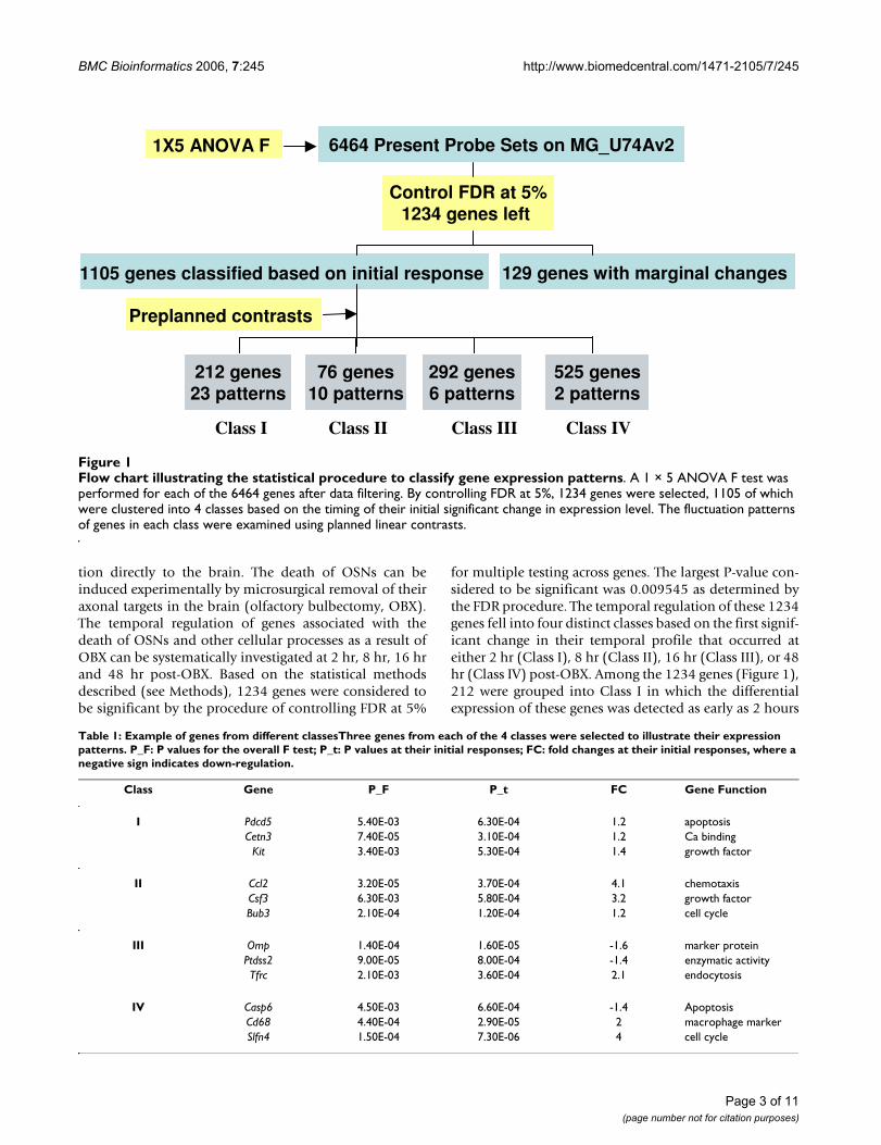
The genes for programmed cell death 5 (Pdcd5), centrin 3(Cetn3), and Kit are examples of Class I genes that showedtheir first significant change in temporal expression at 2 hrpost-OBX, with Pdcd5 and Cetn3 being up-regulated andKit being down-regulated (Figure 3). In contrast, Class IIgenes showed their first significant change in temporalexpression at 16 hr post-OBX (Figure 4); they included thegenes for chemokine (C-C motif) ligand 2 (Ccl2), colonystimulating factor 3 (Csf3), and budding uninhibited bybenzimidazoles 3 homolog (Bub3) that were up-regulatedsimultaneously. The genes for phosphatidylserine syn-thase 2 (Ptdss2) and the transferrin receptor (Tfrc) areexamples of Class III genes that showed their first signifi-
cant change in temporal expression at 16 hr post-OBX,with Ptdss2 and Tfrc down-regulated and up-regulatedrespectively (Figure 5). The genes identified statistically asClass IV genes were initially quiescent until their first sig-nificant change in expression at 48 hr post-OBX (Figure 6)as shown by the genes for caspase 6 (Casp6), CD68 anti-gen (Cd68), and schlafen 4 (Slfn4). From a functional per-spective, the regulation of the genes for Pdcd5, Ptdss2, andCasp6 at 2 hr, 16 hr, and 48 hr respectively suggested thatthe molecular mechanisms associated with OSN degener-ation and cell death occurred over a 2d time frame that isconsistent with the systematic down-regulation of thegene for Omp. The up-regulation of the genes for Ccl2 andCd68 at 8 hr and 48 hr respectively suggested the expres-sion of macrophage chemoattractant protein-1 (CCL2) byresident and recruited macrophages identified phenotypi-cally with CD68 antibody that indicate the delivery of bio-active molecules associated with the earliest regenerationof the sensory epithelium. The genes for Kit, Csf3, Bub3,and Slfn4 are broadly defined as having growth factoractivity, which suggested that molecular mechanismsassociated with the transformation of progenitor cells intomature OSNs through the proliferative stages of the cellcycle was initiated within 2 hr of OBX and continuedthroughout the following 48 hr. The results of our statisti-cal and bioinformatics analyses clearly indicate that thecategorization of genes into four Classes based on theirfirst significant temporal regulatory event has biologicalrelevance at the cellular level in this neurosensory tissue.
Genes in each class share the same timing of their earliestsignificant change in expression. The expression pattern ofeach gene at subsequent time points may vary. We there-fore can further cluster genes in each class into subgroupsbased on their subsequent expression patterns or 'fluctua-tion patterns'. For genes in Class I (Figure 1), there theo-retically may as many as 54 fluctuation patterns. In ourexample study, we found 23 different patterns in thisclass. There were 10, 6, and 2 patterns for genes in Class II,III, and IV respectively. We can use simple diagrams toillustrate these patterns and a series of characters (1, 0, -1)to index their expression patterns as described in theMethods. For example, the fluctuation pattern of Ompexpression (Figure 2) can be represented by (0 0 0 -1 -1),and the expression of Pdcd5 can be indicated by (0 1 0 00) (Figure 3). Genes with the same fluctuation patternswill be finally grouped into the same group (Figure 7). Forexample, gene Cetn2 and Cetn3 shared the same expres-sion pattern and can be grouped together. This patternwas indicated by (0 1 -1 0 -1). Genes Csf3 and Pdcd8 hadtheir initial responses at hr16 and shared the same fluctu-ation pattern. These two genes can be classified intoanother group indicated as (0 0 1 -1 0). Genes CD68 andSlfn4 (Figure 6) can also form a cluster for the same rea-son.
A simple diagram to illustrate the expressionpattern of the gene OmpFigure 2A simple diagram to illustrate the expressionpattern of the gene Omp. Mean hybridization signals (± SD) at each time point were plotted. The expression of Omp was unchanged at 2 hr and 8 hr following OBX. Its first significant change in expression was a down-regulation at 16 hr post-OBX. Its expression continued to decrease at 48 hr. The fluctuation pattern of Omp expression was indexed by (0 0 0 -1 -1), shown in the upper right corner of the graph. Dia-grams in the following figures were plotted similarly.
0 10 20 30 40 50
10000
15000
20000
25000
30000
35000Omp 0 0 0 -1 -1
Time (hr)
Sig
nal
Page 4 of 11(page number not for citation purposes)
DiscussionIn this study, we adopted linear models to describe ourdata and used planned linear contrasts to analyze time-course microarray experiments. We identified 1234 geneswith significant changes in expression in a microarraystudy of murine olfactory epithelium, and 1105 of themwere grouped into 4 classes based on the timing of theirinitial changes. We further categorized these 1105 genesinto 41 fluctuation patterns. We also used simple dia-grams to illustrate these fluctuation patterns and a seriesof characters (1, 0, -1) to index these patterns. Althoughthe ANOVA F tests were significant, 129 genes cannot begrouped into any of these 4 classes based on our criteria.A significant ANOVA F test among a group of means indi-cates that the largest contrast among all possible contrastsis significant. Therefore, a gene with a significant F testdoes not necessarily have a significant selected contrast.Therefore the expression patterns of these genes should beinterpreted carefully.
The critical value used to select significant
contrasts is the uniform upper bound for testing a com-plete set of contrasts regardless of the correlation structureamong these contrasts. It is a conservative approach. Forplanned linear contrasts, the most powerful bound can befound based on the correlation structure of these contrasts[31,32]. In general, the most powerful bound can't beobtained without knowing the correlation structureamong the contrasts [33]. The uniform bound, however,can be obtained from testing a complete set of orthogonalcontrasts using the Studentized Maximum Modulus Dis-tribution [34]. In practice, although a little bit conserva-tive, it is straightforward to use this uniform bound to testall contrasts especially when the number of different com-binations of contrasts is large.
Our methods emphasized the relative differences betweenadjacent sampling time points and the direction of the dif-
Mnew m vα , ,−2
Example diagrams to illustrate expression patterns of genes in Class IFigure 3Example diagrams to illustrate expression patterns of genes in Class I. Mean signals (± SD) for genes Pdcd5, Cetn3, and Kit from Class I were plotted. Their expression levels were significantly altered at as early as 2 hr after OBX. Their subsequent expression patterns were different, which was indicated by the indices in each panel.
0 10 20 30 40 50
5000
6000
7000
8000Pdcd5
0 10 20 30 40 50500
700
900
1100
1300 Kit
0 10 20 30 40 507000
8000
9000
10000
11000
12000
13000Cetn3
0 1 0 0 0
0 1 -1 0 -1
0 -1 0 0 0
Time (hr)
Sig
nal
Sig
nal
Sig
nal
Example diagrams to illustrate expression patterns of genes in Class IIFigure 4Example diagrams to illustrate expression patterns of genes in Class II. Expression patterns of genes Ccl2, Csf3, and Bub3 from Class II were significantly altered initially at 8 hr after OBX, and each of these genes has a different fluctuation index.
0 10 20 30 40 50
0
1000
2000
3000
Csf3
0 10 20 30 40 50
0
400
800
1200Ccl2
0 10 20 30 40 50
3500
4000
4500
5000
5500Bub3
0 0 1 0 1
0 0 1 -1 0
0 0 1 0 -1
Time (hr)
Sig
nal
Sig
nal
Sig
nal
Page 5 of 11(page number not for citation purposes)
ferences. The information about exact magnitudes of geneexpressed at each time point was not included in ourmethods. For example, two genes may have the same pat-tern index 0 1 -1 0 0, but the magnitude of changes for thetwo genes may be dramatically different. Therefore, evenfor genes in the same index groups, their expression pat-terns should be examined with care.
The temporal order in the data was considered in ourmethods by the selection sequence but was not parame-terized in our model. The information about the differ-ences among sampling intervals were also ignored in ouranalysis. With small sample sizes and non-uniform sam-pling intervals, which are very common in biomedicalresearch, our methods may be more straightforward androbust than those commonly in use. With large samplesizes and relative uniform sampling intervals, other meth-ods, such as regression analysis, mixture models, orautoregressive models can be applied.
ConclusionLinear models were adopted to describe microarray data,and sequences of planned linear contrasts were used togroup genes into different expression patterns based ontheir initial and subsequent changes in expression. Ourmethods are particularly suitable for analysis of microar-ray experiments in which it is often difficult to take suffi-ciently frequent measurements and/or the sampling
intervals are non-uniform. Our methods can also beextended to designs with more than one factor.
MethodsMicroarray experimentsThe goal of this study was to investigate the induction ofgene regulation at short time intervals (2, 8, 16, and 48hrs) following deafferentation of olfactory sensory neu-rons by target ablation (olfactory bulbectomy, OBX) com-pared with sham controls [35]. Total RNA was isolatedfrom the olfactory epithelium of 3 male mice per timepoint (1 GeneChip/mouse). Following hybridizationwith Affymetrix GeneChips MG U74Av2, 3 chips per timepoint (a total of 15 GeneChips), the signal intensitieswere generated by Affymetrix Microarray Suite v5.0.
In our study, all positive control genes and genes thatresulted in "absent" calls for all chips across all timepoints were removed from further analysis. If there was noevidence that these genes were expressed in any of thesamples, then these genes can be removed to reduce prob-
Example diagrams to illustrate expression pattern of genes in Class IIIFigure 5Example diagrams to illustrate expression pattern of genes in Class III. Expression patterns of genes Ptdss2, and Tfrc from Class III, which are unchanged at 2 hr and 8 hr, were first significantly altered at 16 hr after OBX, and each had a different fluctuation index.
0 10 20 30 40 50
1000
1500
2000
2500
3000
3500 Ptdss2
0 10 20 30 40 50
0
500
1000
1500Trfr
Time (hr)
Sig
nal
Sig
nal
0 0 0 -1 0
0 0 0 1 0
Example diagrams to illustrate expression patterns of genes in Class IVFigure 6Example diagrams to illustrate expression patterns of genes in Class IV. Expression patterns of genes Casp6, Cd68 and Slfn4 from Class IV, were unchanged until the last time point sampled, 48 hr after OBX.
0 10 20 30 40 50
500
900
1300
1700
Casp6
0 10 20 30 40 50
500
1000
1500
2000
2500
Cd68
0 10 20 30 40 50
0
500
1000
1500
Slfn4
Time (hr)
Sig
nal
Sig
nal
Sig
nal
0 0 0 0 -1
0 0 0 0 1
0 0 0 0 1
Page 6 of 11(page number not for citation purposes)
lems associated with multiple comparisons. Other meth-ods of removing low intensity points were also suggestedby Bolstad et al., 2003[36]. All ESTs were also removedfrom the analysis because the primary aim of these exper-iments was to identify known genes that were differen-tially regulated; eliminating ESTs further reducedproblems with multiple comparisons. After data filteringsteps, 6464 genes remained, and the background-cor-rected intensities of these genes were subjected to furtherstatistical analyses.
Algorithm and analysisStatistical modelWe use a linear model to describe the experiment. Let Ygbe the vector of observed expression levels for gene g, g =1, ..., 6464 then
Yg = Xβg + εg
where X is the matrix of known constants, βg = (µg1, µg2, ...,µgm), and m is the number of time points (m = 5 in thisstudy). εg is the random error, and we assume εg ~ MVN(0,σg
2I).
Reverse Helmert seriesA contrast is a linear combination of parameters for whichthe coefficients sum to zero. A complete set of orthogonalcontrasts is a set of k-1 contrasts in k treatments (or treat-ment combinations) which provides a complete parti-tioning of the variability among parameters into mutuallyexclusive and exhaustive parts. Each contrast in such a setis orthogonal to every other remaining one [37]. Onecommonly used complete set of orthogonal contrasts isthe reverse Helmert series, in which one treatment groupis compared with the average of all remaining treatmentgroups. Subsequent contrasts eliminate the first group andthen proceed by comparing one of the remaining groupsto the average of the other remaining groups, as showbelow:
One of the advantages of the Reverse Helmert contrasts isthat these contrasts are orthogonal and, hence, contrastsamong the sample means are uncorrelated. Basing tests onuncorrelated contrasts avoids the problems inherent ininterpreting conditional tests. Adjacent Differences(AD)are sometimes used to identify the point at which initialgene expression occurs. However, these contrasts are notorthogonal and consecutive contrasts have a correlationof 0.5. Consequently, the probability of identifying thecorrect threshold is lower for AD than for the ReverseHelmert Contrasts.
Lββ =
−
−
− − −−
1 1 0 0
12
12
1 0
0
11
11
11
1
1.
.
. . . .
.m m m
µµ22
.
.
µm
Genes shared the same expression pattern were grouped togetherFigure 7Genes shared the same expression pattern were grouped together. Expression patterns of genes Cetn2 and Cetn3 from Class I are the same and therefore they were grouped together. Another example is genes Csf3 and Pdcd8 from Class II which were put into one group because of the same expression pattern.
Cetn2 0 1 -1 0 -1
0 10 20 30 40 50
7000
8000
9000
10000
11000
12000
13000 Cetn3 0 1 -1 0 -1
Csf3 0 0 1 -1 0
0 10 20 30 40 50
2000
2500
3000
3500
4000Pdcd8 0 0 1 -1 0
Sig
nal
Sig
nal
Sig
nal
Sig
nal
0 10 20 30 40 50
1000
1500
2000
2500
3000
0 10 20 30 40 50
0
1000
2000
3000
Time (hr)
Page 7 of 11(page number not for citation purposes)
Clustering genes based on the timing of their initial responsesThe reverse Helmert series can test the following m-1hypotheses sequentially:
Genes will be partitioned into m-1 classes based on thetesting results of H10 ~ Hs0, where s = m-1. Class 1 containsgenes that reject H10; genes that reject H20 from theremaining list are grouped into class 2, and so on; Class sincludes genes that reject Hs0 without rejecting the previ-ous s-1 hypotheses. Therefore Genes in Class 1 are consid-ered to be early responding genes whose expression levelsare significantly altered during the first sampling interval,that is, at the 2nd sampling time point. Genes that do notchange their expression levels until the 3rd sampling timepoint are collected in Class 2, and so on. As indicated bythe described partition process, genes within a class sharethe same timing of onset or cessation of expression.
Clustering genes within a classGenes in each of these above m-1 classes can be furtherclassified based on their 'fluctuation' shapes at the subse-quent sampling points. For gene g in class j, where j = 1, 2,..., s, the following s-j contrasts are needed,
Therefore, a specific sequence of m-1 hypotheses will beperformed for each gene to determine its expression pat-
tern. Let be the unbiased estimate of the contrast cor-
responding to the hypothesis , in a balanced
experiment with sample size n in each treatment group,the statistic
where ci is the ith coefficient for the contrast, and i = 1, ...,
m. MSEg is the usual unbiased estimate of , and v = N-
m is the error degree of freedom (df), where N = mn.
Indexing gene expression patternsLet the state of the first observation be 0, for gene g, itsexpression profile can be transformed into a sequence ofexpression fluctuation as follows:
where k = 1, 2, ..., s is an index, where k = r if it is the rthcontrast for gene g. S is the transformed value of the geneexpression profiles. Thus an m-time-point expression pro-file is transformed into an m-1-state sequence of expres-sion fluctuation consisting of a character set (1, 0, -1).Each character in the sequence indicates whether themean expression level of the gene is significantly up-regu-lated (1), not altered (0), or significantly down-regulated(-1) at the next time point, while the whole sequence rep-resents the fluctuation pattern of the gene expression.Besides the pattern in which the gene's expression level isunchanged throughout the entire sampling period, thereare at most 2 × 3m-k-1 fluctuation patterns for genes in Classk. There are no more than 3m-1 patterns of expression intotal in an m-time-point microarray experiment.
Multiple testing controlAn ANOVA F test was performed for each gene to identifythe differentially expressed genes. This F test is testing thehypothesis µg1 = µg2, ..., = µgm, which is equivalent to testthe composite hypothesis Lβ = 0. The BH procedure ofcontrolling FDR at 5% was applied to the P values of theF test. A cutoff point αnew, which is equal to the largest Pvalue considered to be significant, was determined by theabove BH procedure. By this procedure, each test for thegene that rejected the F test is at least αnew level test.
For each selected gene, a specific sequence of m-1 con-trasts was tested to determine its expression pattern. To beconsistent with the BH procedure performed, the family-wise error rates (FWER) for these genes have to be control-led at least at the level of αnew. In this study, we controlledthe maximum family-wise error rates (MFWER) by usingthe Studentized Maximum Modulus distribution [34].The following theorem in the Appendix outlined the con-cern of gene-based controlling MFWER at the level of αnew.
Outline of the analysisA short summary of the statistical methods used in thisstudy follows:
H
H
Hms
mm
10 1 2
201 2
3
01 2 1
0
20
1
:
:
........
:...
µ µµ µ µ
µ µ µ µ
− =+ − =
+ + +−
−− == 0
Hgj
gj
gj, :1 1 2 0µ µ+ +− =
H
H
gj k
gj k
gj k
gj k
gj k
gj k
gJ k
,
,
:
µ µ
µ µµ
+ + + −
+ − +=
− =
+−
1 1
1
0
2
if reject
++ −=
= −1 10 if fail to reject H
k s j
gj k,
,2…
ˆ ,λgj k
Hgj k,
T
MSE
c
n
gj k g
j k
g
igi
m,
,
~=
=∑
λ
2
1
tv
σ g2
S
if reject and
if or fail tgj k
gj k
gj kk j H
k j,
, ,, ,
=
≥ <
<
1 0
0
λ
oo reject
if reject and
H
k j H
gj k
gj k
gj k
,
, ,, ,− ≥ >
1 0λ
= =j s k s1 1, , , , ,… …
Page 8 of 11(page number not for citation purposes)
1. Linear models were used to describe the data based onthe experimental design. For each gene, an ANOVA F testwas performed based on the described model, and thecorresponding P-value was obtained.
2. To adjust for multiple tests based on the large numberof genes, the BH method of controlling FDR [22] at 5%was applied to the P-values obtained above, providing alist of genes (list I) that exhibit significant differencesamong the means of the 5 sampling points.
3. Using αnew, which equals the largest P-value determined
to be significant in step 2 as the cut-off point, we groupedgenes in list I into 4 classes based on the timing of theirinitial responses by testing the reverse Helmert contrastssequentially. The Studentized Maximum Modulus distri-bution parameter m-2 = 3 and v = 10 were used in this
example study, where αnew = 0.009545 and
= |M0.009545,3,10| = 3.8651.
4. Using the same critical value , we further
clustered genes in each of the above classes by testingappropriate contrasts for the subsequent sampling timepoints.
5. Based on the results of the m-1 contrasts for each gene,we also can select genes which share similar pattern ofexpression for any number of sampling intervals from thebeginning.
Statistical softwareWe used the SAS (version 9.0) proc GLM procedure to domodel fitting and significance analysis. The SAS programimplementing linear models for the olfactory sensory epi-thelia data is available [38].
Authors' contributionsHL carried out the statistical analyses and formulation ofstatistical methods. YL automized the statistical analysisusing Splus/R. TVG and MLG carried out the moleculargenetics studies. CLW and AJS supervised the study. Allauthors contributed to the writing of this manuscript. Allauthors read and approved the final manuscript.
AppendixTheorem For any balanced one-way model with m treat-ment groups and assuming normality and equal varianceσ2, Let λ1, λ2, ..., λk be an arbitrary complete set of con-trasts such that
Under the null hypothesis, let P be the distribution of the
vector λ = [λ1, λ2, ..., λK] with mean 0 and covariance
matrix ∑, let PK be the distribution of the vector of a com-
plete set of contrasts with the covari-
ance matrix ∑K = Iσ2 is the diagonal of ∑ then the gene
based maximum family-wised error rate (MFWER) at any
level of α of testing a specific sequence of contrasts (list inthe Methods) after rejecting the overall F test is achievedby comparing |Ti| with |Mα,k-1,v|, where v is the df of error,
and |Mα,k-1,v| is the 100(1 - α) percentile from the Studen-tized Maximum Modulus distribution.
Proof Let λ1, λ2, ..., λK be any complete set of contrasts,then let
V0 = {0 ≤ i ≤ K: λi = 0} and
V1 = {0 ≤ j ≤ K: λj ≠ 0},
let test function
(1) Suppose V1 is empty such that λi = 0 ∀i, then MFWERis
(2) V0 is empty such that λi ≠ 0 ∀i, then MFWER is 0.
Mnew m vα , ,−2
Mnew m vα , ,−2
λ µi i ii
mc i K= =
=∑ , , , ,1 2
1
…
λλ* = [ , , , ]* * *λ λ λ1 2 … K
T
MSE
c
n
ii
ii
m=
=∑
λ̂
2
1
φ λλ
λii i
i i
H
H( ) =
=1 0
00
0
if reject the
if fail to reject the
:
: == 0
MFWER
= { }
=
Pr
Pr ( ( (
at least one false reject
F test rejected) φ λλ
α
ii V
) )
Pr
=
≤ { }≤
∈1
0
∪∩
F test rejected
Page 9 of 11(page number not for citation purposes)
(3) Suppose that neither V0 nor V1 is empty, then MFWERis
under PK, based on Sidak's inequality (8) [39],
has a Studentized Maximum Modulus dis-
tribution [34] with parameter K-1 and v, let
MFWER = α*(α, m - 1, v) = max{α(α, m - 1, v)} = α,
then q = |Mα,K-1,v| is the 100(1-α) percentile from abovedistribution.
AcknowledgementsThis work was supported by NIH AG-016824 (TVG) and NIH-P20RR16481 and NSF-EPS-0132295 (AJS). We also wish to thank Donna Wall, Microarray Core Facility, and Radhika Vaishnav, M.S., Department of Physiology, for their expertise.
4. Garrity GM, Lilburn TG: Self-organizing and self-correctingclassifications of biological data. Bioinformatics 2005,21(10):2309-2314.
5. Brown MPS, Grundy WN, Lin D, Cristianini N, Sugnet CW, Furey TS,Ares M Jr, Haussler D: Knowledge-based analysis of microarraygene expression data by using support vector machines.PNAS 2000, 97(1):262-267.
7. Bar-Joseph Z, Gerber G, Giord DK, Jaakkola TS, Simon I: A newapproach to analyzing gene expression time series data. Pro-ceedings of RECOMB, Washington DC, USA 2002:39-48.
8. Park T, Yi S-G, Lee S, Lee SY, Yoo D-H, Ahn J-I, Lee Y-S: Statisticaltests for identifying differentially expressed genes in time-course microarray experiments. Bioinformatics 2003,19(6):694-703.
9. Ramoni MF, Sebastiani P, Kohane IS: From the Cover: Clusteranalysis of gene expression dynamics. PNAS 2002,99(14):9121-9126.
10. Sasik R, Iranfar N, Hwa T, Loomis WF: Extracting transcriptionalevents from temporal gene expression patterns during Dic-tyostelium development. Bioinformatics 2002, 18(1):61-66.
11. Ji X, Li-Ling J, Sun Z: Mining gene expression data using a novelapproach based on hidden Markov models. FEBS Letters 2003,542(1–3):125-131.
12. Schliep A, Schönhuth A, Steinhoff C: Using hidden Markov mod-els to analyze gene expression time course data. Bioinformatics2003, 19(90001):i255-263.
13. Yeung KY, Bumgarner RE, Raftery AE: Bayesian model averaging:development of an improved multi-class, gene selection andclassification tool for microarray data. Bioinformatics 2005,21(10):2394-2402.
14. Peddada SD, Lobenhofer EK, Li L, Afshari CA, Weinberg CR, UmbachDM: Gene selection and clustering for time-course and dose-response microarray experiments using order-restrictedinference. Bioinformatics 2003, 19(7):834-841.
15. Bensmail H, Celeux G, Raftery AE, Robert CP: Inference in model-based cluster analysis. Statistics and Computing 1997, 7:1-10.
16. Yeung KY, Fraley C, Murua A, Raftery AE, Ruzzo WL: Model-basedclustering and data transformations for gene expressiondata. Bioinformatics 2001, 17(10):977-987.
17. Fraley C, Raftery AE: How many clusters? Which clusteringmethod? Answers via model-based cluster analysis. ComputerJournal 1998, 41:578-588.
18. Medvedovic M, Sivaganesan S: Bayesian infinite mixture modelbased clustering of gene expression profiles. Bioinformatics2002, 18(9):1194-1206.
19. Pan W, Lin J, Le C: Model-based cluster analysis of microarraygene-expression data. Genome Biology 2002,3(2):research0009.0001-research0009.0008.
21. Moller-Levet CS, Cho KH, Wolkenhauer O: Microarray data clus-tering based on temporal variation: FCV with TSD preclus-tering. Appl Bioinformatics 2003, 2(1):35-45.
22. Benjamini Y, Hochberg Y: Controlling the false discovery rate: apractical and powerful approach to multiple testing. JRoy StatSoc 1995, B(75):289-300.
23. Benjamini Y, Yekutieli D: The control of the false discovery rateunder dependency. Ann Stat 2001, 29:1165-1188.
24. Benjamini Y, Yekutieli D: Quantitative Trait Loci Analysis usingthe False Discovery Rate. Genetics 2005. genetics.104.036699
25. Efron B, Tibshirani R, Storey JD, Tusher V: Empirical Bayes analy-sis of a microarray experiment. J Am Stat Assoc 2001,96:1151-1160.
26. Storey JD: The positive false discovery rate: A Bayesian inter-pretation and the Q-Value. Technical Report 2001–12.Department of Statistics, Stanford University. 2001.
27. Reiner A, Yekutieli D, Benjamini Y: Identifying differentiallyexpressed genes using false discovery rate controlling proce-dures. Bioinformatics 2003, 19(3):368-375.
28. Grant GR, Liu J, Stoeckert CJ Jr: A practical false discovery rateapproach to identifying patterns of differential expression inmicroarray data. Bioinformatics 2005, 21(11):2684-2690.
29. Pawitan Y, Michiels S, Koscielny S, Gusnanto A, Ploner A: False dis-covery rate, sensitivity and sample size for microarray stud-ies. Bioinformatics 2005, 21(13):3017-3024.
30. Li H, Wood C, Getchell T, Getchell M, Stromberg A: Analysis of oli-gonucleotide array experiments with repeated measuresusing mixed models. BMC Bioinformatics 2004, 5(1):209.
31. Nelson PR: Multivariate normal and t distributions with Pjk =αjαk. Commun Stat Simulation & computation 1982, 11:239-248.
MFWER
= { }
=
Pr
Pr (
at least one false rejection
F test rejected) (( ( ) )
Pr ( )
Pr (
φ λ
φ λ
φ λ
ii V
ii V
i
=
≤ =
≤
∈
∈
1
1
0
0
∪∩
∪
)),
=
∈ = −1
0 0 1i V v K
v∪ where is the number of eleme0 nnts in and V v K
ii V v K
0 0
1
1
1 00 0
max
Pr ( ),
( ) = −
= − =
∈ = −φ λ∩
= − ≤
≤ − ≤
∈ = −
∈ =
1
1
0 0
0 0
1
P T q
P T q
ii V v K
K ii V v
,
,
∩
KK
Ki
P
−
∈
≤ −
1
1
∩ by Sidak’s inequality (1967,(8))
maxVV v K
i
Ki V v K
i
Ki V
T q
P T q
P
0 0
0 0
1
11
,
,max
max
= −
∈ = −
∈
≤
≤ − ≤
=00 0 1,v K
iT q= −
≥
max,i V v K
iT∈ = −0 0 1
Page 10 of 11(page number not for citation purposes)
Publish with BioMed Central and every scientist can read your work free of charge
"BioMed Central will be the most significant development for disseminating the results of biomedical research in our lifetime."
Sir Paul Nurse, Cancer Research UK
Your research papers will be:
available free of charge to the entire biomedical community
peer reviewed and published immediately upon acceptance
cited in PubMed and archived on PubMed Central
yours — you keep the copyright
Submit your manuscript here:http://www.biomedcentral.com/info/publishing_adv.asp
BioMedcentral
32. Kirk RE: Experimental Design: Procedures for the BehavioralSciences. Belmont, CA: Brooks/Cole; 1982:92.
33. Wilcox RR: New designs in analysis of variance. Ann Rev Psychol1987, 38:29-60.
34. Bechhofer RE, Dunnett CW: Multiple comparisons for orthogo-nal contrasts: example and table. Technometrics 1982,24:213-222.
35. Getchell TV, Liu H, Vaishnav RA, Kwong K, Stromberg AJ, GetchellML: Temporal profiling of gene expression during neurogen-esis and remodeling in the olfactory epithelium at shortintervals after target ablation. Journal of Neuroscience Research2005, 80(3):309-329.
36. Bolstad BM, Irizarry RA, Astrand M, Speed TP: A comparison ofnormalization methods for high density oligonucleotidearray data based on variance and bias. Bioinformatics 2003,19(2):185-193.
37. Klockars AJ, Hancock GR: Power of recent multiple comparisonprocedures as applied to a complete set of planned orthogo-nal contrasts. Psychological Bulletin 1992, 111(3):505-510.
38. Contrast [http://www.mc.uky.edu/UKMicroArray/contrast.txt]39. Sidak Z: Rectangular Confidence Regions for the Means of
Multivariate Normal Distributions. Am Stat Asso 1967,62:626-633.
Page 11 of 11(page number not for citation purposes)