Identification of one-parameter bifurcations giving rise to periodic orbits, from their period function Armengol Gasull 1 , V´ ıctor Ma ˜ nosa 2 , and Jordi Villadelprat 3 1 Departament de Matem ` atiques Universitat Aut` onoma de Barcelona 2 Departament de Matem ` atica Aplicada III Control, Dynamics and Applications Group (CoDALab) Universitat Polit` ecnica de Catalunya. 3 Departament d’Enginyeria Inform ` atica i Matem ` atiques Universitat Rovira i Virgili. 15th International Workshop on Dynamics and Control. May 31–June 3, 2009, Tossa de Mar, Spain. Gasull,Ma ˜ nosa,Villadelprat (UAB-UPC-URV) Identification of Bifurcations Dynamics & Control 1 / 18
Transcript
Identification of one-parameter bifurcations givingrise to periodic orbits, from their period function
Armengol Gasull1, Vıctor Manosa2, and Jordi Villadelprat3
1Departament de MatematiquesUniversitat Autonoma de Barcelona
2Departament de Matematica Aplicada IIIControl, Dynamics and Applications Group (CoDALab)
Universitat Politecnica de Catalunya.
3Departament d’Enginyeria Informatica i MatematiquesUniversitat Rovira i Virgili.
15th International Workshop on Dynamics and Control.May 31–June 3, 2009, Tossa de Mar, Spain.
Gasull,Manosa,Villadelprat (UAB-UPC-URV) Identification of Bifurcations Dynamics & Control 1 / 18
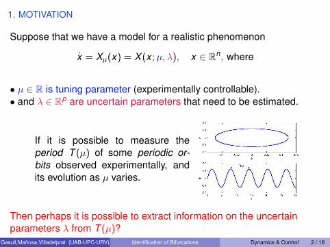
1. MOTIVATION
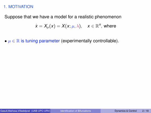
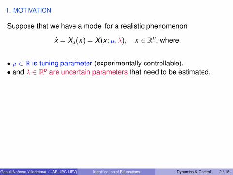
Suppose that we have a model for a realistic phenomenon
x = Xµ(x) = X (x ;µ, λ), x ∈ Rn, where
• µ ∈ R is tuning parameter (experimentally controllable).• and λ ∈ Rp are uncertain parameters that need to be estimated.
If it is possible to measure theperiod T (µ) of some periodic or-bits observed experimentally, andits evolution as µ varies.
Then perhaps it is possible to extract information on the uncertainparameters λ from T (µ)?
Gasull,Manosa,Villadelprat (UAB-UPC-URV) Identification of Bifurcations Dynamics & Control 2 / 18
1. MOTIVATION
Suppose that we have a model for a realistic phenomenon
x = Xµ(x) = X (x ;µ, λ), x ∈ Rn, where
• µ ∈ R is tuning parameter (experimentally controllable).
• and λ ∈ Rp are uncertain parameters that need to be estimated.
If it is possible to measure theperiod T (µ) of some periodic or-bits observed experimentally, andits evolution as µ varies.
Then perhaps it is possible to extract information on the uncertainparameters λ from T (µ)?
Gasull,Manosa,Villadelprat (UAB-UPC-URV) Identification of Bifurcations Dynamics & Control 2 / 18
1. MOTIVATION
Suppose that we have a model for a realistic phenomenon
x = Xµ(x) = X (x ;µ, λ), x ∈ Rn, where
• µ ∈ R is tuning parameter (experimentally controllable).• and λ ∈ Rp are uncertain parameters that need to be estimated.
If it is possible to measure theperiod T (µ) of some periodic or-bits observed experimentally, andits evolution as µ varies.
Then perhaps it is possible to extract information on the uncertainparameters λ from T (µ)?
Gasull,Manosa,Villadelprat (UAB-UPC-URV) Identification of Bifurcations Dynamics & Control 2 / 18
1. MOTIVATION
Suppose that we have a model for a realistic phenomenon
x = Xµ(x) = X (x ;µ, λ), x ∈ Rn, where
• µ ∈ R is tuning parameter (experimentally controllable).• and λ ∈ Rp are uncertain parameters that need to be estimated.
If it is possible to measure theperiod T (µ) of some periodic or-bits observed experimentally, andits evolution as µ varies.
Then perhaps it is possible to extract information on the uncertainparameters λ from T (µ)?
Gasull,Manosa,Villadelprat (UAB-UPC-URV) Identification of Bifurcations Dynamics & Control 2 / 18
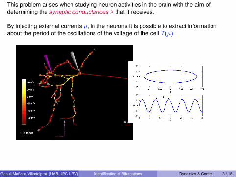
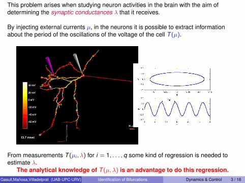
This problem arises when studying neuron activities in the brain with the aim ofdetermining the synaptic conductances λ that it receives.
By injecting external currents µ, in the neurons it is possible to extract informationabout the period of the oscillations of the voltage of the cell T (µ).
From measurements T (µi , λ) for i = 1, . . . , q some kind of regression is needed toestimate λ.
The analytical knowledge of T (µ, λ) is an advantage to do this regression.
Gasull,Manosa,Villadelprat (UAB-UPC-URV) Identification of Bifurcations Dynamics & Control 3 / 18
This problem arises when studying neuron activities in the brain with the aim ofdetermining the synaptic conductances λ that it receives.
By injecting external currents µ, in the neurons it is possible to extract informationabout the period of the oscillations of the voltage of the cell T (µ).
From measurements T (µi , λ) for i = 1, . . . , q some kind of regression is needed toestimate λ.
The analytical knowledge of T (µ, λ) is an advantage to do this regression.Gasull,Manosa,Villadelprat (UAB-UPC-URV) Identification of Bifurcations Dynamics & Control 3 / 18
2. STARTING POINT
From the knowledge T (µ) of a one parameter family of P.O. it is possible to identifythe type of bifurcation which has originated the P.O.?
YES ⇒ important restrictions on the uncertainties λ∈ Rp to be estimated⇒ better knowledge of the model.
—————————————————————
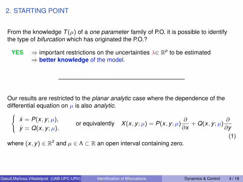
Our results are restricted to the planar analytic case where the dependence of thedifferential equation on µ is also analytic.{
x = P(x , y ;µ),
y = Q(x , y ;µ).or equivalently X (x , y ;µ) = P(x , y ;µ)
∂
∂x+ Q(x , y ;µ)
∂
∂y(1)
where (x , y) ∈ R2 and µ ∈ Λ ⊂ R an open interval containing zero.Our objective is to relate the form of T (µ) with the type of bifurcation of limitcycles.
Gasull,Manosa,Villadelprat (UAB-UPC-URV) Identification of Bifurcations Dynamics & Control 4 / 18
2. STARTING POINT
From the knowledge T (µ) of a one parameter family of P.O. it is possible to identifythe type of bifurcation which has originated the P.O.?
YES ⇒ important restrictions on the uncertainties λ∈ Rp to be estimated⇒ better knowledge of the model.
—————————————————————
Our results are restricted to the planar analytic case where the dependence of thedifferential equation on µ is also analytic.{
x = P(x , y ;µ),
y = Q(x , y ;µ).or equivalently X (x , y ;µ) = P(x , y ;µ)
∂
∂x+ Q(x , y ;µ)
∂
∂y(1)
where (x , y) ∈ R2 and µ ∈ Λ ⊂ R an open interval containing zero.
Our objective is to relate the form of T (µ) with the type of bifurcation of limitcycles.
Gasull,Manosa,Villadelprat (UAB-UPC-URV) Identification of Bifurcations Dynamics & Control 4 / 18
2. STARTING POINT
From the knowledge T (µ) of a one parameter family of P.O. it is possible to identifythe type of bifurcation which has originated the P.O.?
YES ⇒ important restrictions on the uncertainties λ∈ Rp to be estimated⇒ better knowledge of the model.
—————————————————————
Our results are restricted to the planar analytic case where the dependence of thedifferential equation on µ is also analytic.{
x = P(x , y ;µ),
y = Q(x , y ;µ).or equivalently X (x , y ;µ) = P(x , y ;µ)
∂
∂x+ Q(x , y ;µ)
∂
∂y(1)
where (x , y) ∈ R2 and µ ∈ Λ ⊂ R an open interval containing zero.Our objective is to relate the form of T (µ) with the type of bifurcation of limitcycles.
Gasull,Manosa,Villadelprat (UAB-UPC-URV) Identification of Bifurcations Dynamics & Control 4 / 18
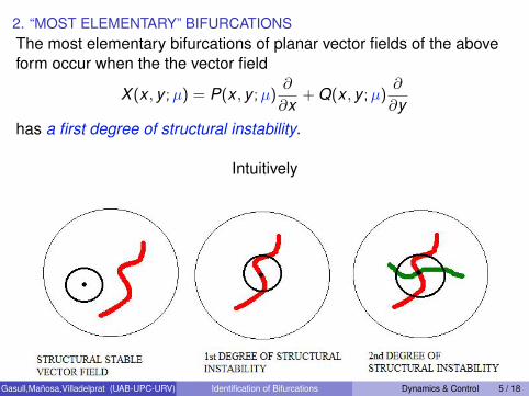
2. “MOST ELEMENTARY” BIFURCATIONSThe most elementary bifurcations of planar vector fields of the aboveform occur when the the vector field
X (x , y ;µ) = P(x , y ;µ)∂
∂x+ Q(x , y ;µ)
∂
∂yhas a first degree of structural instability.
Intuitively
Gasull,Manosa,Villadelprat (UAB-UPC-URV) Identification of Bifurcations Dynamics & Control 5 / 18
All the possible bifurcations that can occur for a vector field with a 1stdegree of structural instability are known (Andronov et al. 1973 andSotomayor 1974)
Among them we only study the isolated ones that give rise to isolatedperiodic orbits (P.O.).
Elementary bifurcations giving rise to P.O.(a) Hopf bifurcation.(b) Bifurcation from semi–stable periodic orbit.(c) Saddle-node bifurcation(d) Saddle loop bifurcation.
We will characterize the asymptotic expansion of the period of theemerging P.O.
Gasull,Manosa,Villadelprat (UAB-UPC-URV) Identification of Bifurcations Dynamics & Control 6 / 18
3. SUMMARY OF OUR RESULTS
“Theorem”:
Generically the form of T (µ) characterizes thetype of bifurcationUnder the conditions that give rise to a bifurcation of P.O. we have
• Hopf bifurcation: T (µ) = T0 + T1µ+ O(|µ|3/2), with T0 > 0 but T1 canbe 0.
• Bifurcation from semi–stable periodic orbit:T±(µ) = T0 ± T1
√|µ|+ O(µ), with T0 > 0 but T1 can be 0.
• Saddle-node bifurcation: T (µ) ∼ T0/√µ(∗)
• Saddle loop bifurcation: T (µ) = c ln |µ|+ O(1), with c 6= 0.
(∗) Where T (µ) ∼ a + f (µ) means that limµ→0
T (µ)− af (µ)
= 1.
Gasull,Manosa,Villadelprat (UAB-UPC-URV) Identification of Bifurcations Dynamics & Control 7 / 18
3. SUMMARY OF OUR RESULTS
“Theorem”: Generically the form of T (µ) characterizes thetype of bifurcation
Under the conditions that give rise to a bifurcation of P.O. we have
• Hopf bifurcation: T (µ) = T0 + T1µ+ O(|µ|3/2), with T0 > 0 but T1 canbe 0.
• Bifurcation from semi–stable periodic orbit:T±(µ) = T0 ± T1
√|µ|+ O(µ), with T0 > 0 but T1 can be 0.
• Saddle-node bifurcation: T (µ) ∼ T0/√µ(∗)
• Saddle loop bifurcation: T (µ) = c ln |µ|+ O(1), with c 6= 0.
(∗) Where T (µ) ∼ a + f (µ) means that limµ→0
T (µ)− af (µ)
= 1.
Gasull,Manosa,Villadelprat (UAB-UPC-URV) Identification of Bifurcations Dynamics & Control 7 / 18
3. SUMMARY OF OUR RESULTS
“Theorem”: Generically the form of T (µ) characterizes thetype of bifurcationUnder the conditions that give rise to a bifurcation of P.O. we have
• Hopf bifurcation: T (µ) = T0 + T1µ+ O(|µ|3/2), with T0 > 0 but T1 canbe 0.
• Bifurcation from semi–stable periodic orbit:T±(µ) = T0 ± T1
√|µ|+ O(µ), with T0 > 0 but T1 can be 0.
• Saddle-node bifurcation: T (µ) ∼ T0/√µ(∗)
• Saddle loop bifurcation: T (µ) = c ln |µ|+ O(1), with c 6= 0.
(∗) Where T (µ) ∼ a + f (µ) means that limµ→0
T (µ)− af (µ)
= 1.
Gasull,Manosa,Villadelprat (UAB-UPC-URV) Identification of Bifurcations Dynamics & Control 7 / 18
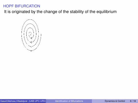
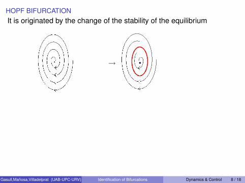
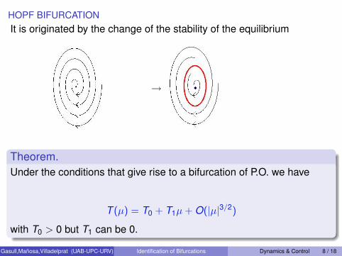
HOPF BIFURCATIONIt is originated by the change of the stability of the equilibrium
→
Theorem.Under the conditions that give rise to a bifurcation of P.O. we have
T (µ) = T0 + T1µ+ O(|µ|3/2)
with T0 > 0 but T1 can be 0.
Gasull,Manosa,Villadelprat (UAB-UPC-URV) Identification of Bifurcations Dynamics & Control 8 / 18
BIFURCATION FROM SEMI–STABLE PERIODIC ORBIT ...my preferred one.
Theorem.Under the conditions that give rise to a bifurcation of P.O. we have
T±(µ) = T0 ± T1√|µ|+ O(µ)
with T0 > 0 but T1 can be 0.
Gasull,Manosa,Villadelprat (UAB-UPC-URV) Identification of Bifurcations Dynamics & Control 9 / 18
BIFURCATION FROM SEMI–STABLE PERIODIC ORBIT ...my preferred one.
Theorem.Under the conditions that give rise to a bifurcation of P.O. we have
T±(µ) = T0 ± T1√|µ|+ O(µ)
with T0 > 0 but T1 can be 0.
Gasull,Manosa,Villadelprat (UAB-UPC-URV) Identification of Bifurcations Dynamics & Control 9 / 18
BIFURCATION FROM SEMI–STABLE PERIODIC ORBIT ...my preferred one.
Theorem.Under the conditions that give rise to a bifurcation of P.O. we have
T±(µ) = T0 ± T1√|µ|+ O(µ)
with T0 > 0 but T1 can be 0.
Gasull,Manosa,Villadelprat (UAB-UPC-URV) Identification of Bifurcations Dynamics & Control 9 / 18
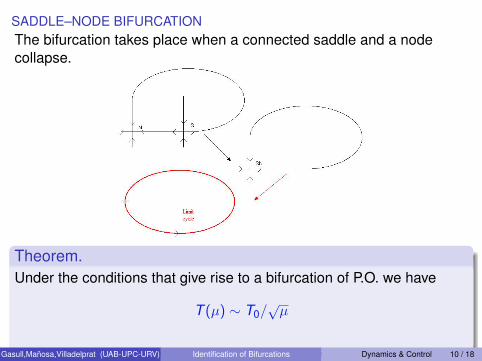
SADDLE–NODE BIFURCATIONThe bifurcation takes place when a connected saddle and a nodecollapse.
Theorem.Under the conditions that give rise to a bifurcation of P.O. we have
T (µ) ∼ T0/√µ
Gasull,Manosa,Villadelprat (UAB-UPC-URV) Identification of Bifurcations Dynamics & Control 10 / 18
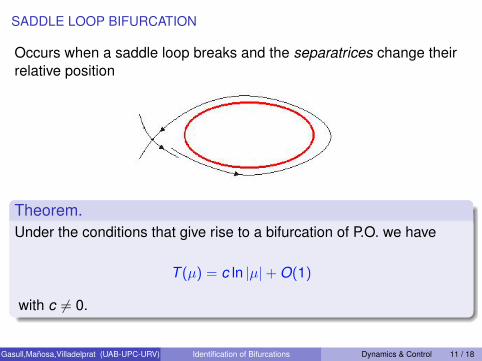
SADDLE LOOP BIFURCATION
Occurs when a saddle loop breaks and the separatrices change theirrelative position
Theorem.Under the conditions that give rise to a bifurcation of P.O. we have
T (µ) = c ln |µ|+ O(1)
with c 6= 0.
Gasull,Manosa,Villadelprat (UAB-UPC-URV) Identification of Bifurcations Dynamics & Control 11 / 18
4. WHAT ABOUT THE PROOFS?
(a) Hopf bifurcation. Usual arguments using polar coordinates, Taylordevelopments, and variational equations.
(b) Bifurcation from semi–stable periodic orbit. Try to reduce theproblem to the Hopf bifurcation framework, but instead of usingpolar coordinates using specific local coordinates (Ye et al. 1983)
(c) Saddle-node bifurcation. Work with normal form theory(Il’yashenko, Li. 1999)
(d) Saddle loop bifurcation. Usual arguments+Normal forms but theframework is very different because the structure of the transitionmaps of the flow, and the transit time functions areNON–DIFFERENTIABLE!
Gasull,Manosa,Villadelprat (UAB-UPC-URV) Identification of Bifurcations Dynamics & Control 12 / 18
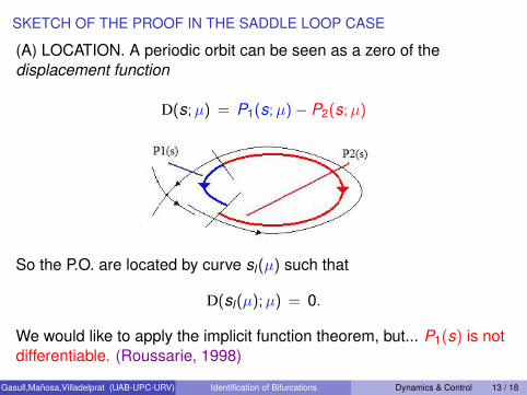
SKETCH OF THE PROOF IN THE SADDLE LOOP CASE
(A) LOCATION. A periodic orbit can be seen as a zero of thedisplacement function
D(s;µ) = P1(s;µ)− P2(s;µ)
So the P.O. are located by curve sl(µ) such that
D(sl(µ);µ) = 0.
We would like to apply the implicit function theorem, but... P1(s) is notdifferentiable. (Roussarie, 1998)
Gasull,Manosa,Villadelprat (UAB-UPC-URV) Identification of Bifurcations Dynamics & Control 13 / 18
(B) TRANSIT TIME ANALYSIS.
The flying time for any orbit can be decomposed as
T (s;µ) = T1(s;µ) + T2(s;µ)
So the period of each limit cycle is given by
T (µ) = T (sl(µ);µ) = T1(sl(µ);µ) + T2(sl(µ);µ)
But... T1(s) is also non–differentiable. (Broer, Roussarie, Simo, 1996)
Gasull,Manosa,Villadelprat (UAB-UPC-URV) Identification of Bifurcations Dynamics & Control 14 / 18
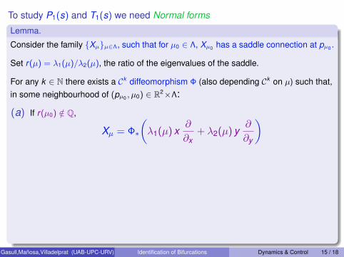
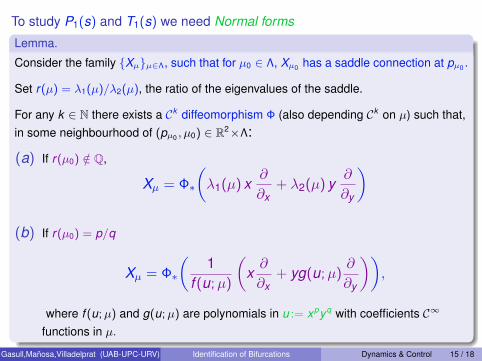
To study P1(s) and T1(s) we need Normal forms
Lemma.
Consider the family {Xµ}µ∈Λ, such that for µ0 ∈ Λ, Xµ0 has a saddle connection at pµ0 .
Set r(µ) = λ1(µ)/λ2(µ), the ratio of the eigenvalues of the saddle.
For any k ∈ N there exists a Ck diffeomorphism Φ (also depending Ck on µ) such that,in some neighbourhood of (pµ0 , µ0) ∈ R2×Λ:
(a) If r(µ0) /∈ Q,
Xµ = Φ∗
(λ1(µ) x
∂
∂x+ λ2(µ) y
∂
∂y
)
(b) If r(µ0) = p/q
Xµ = Φ∗
(1
f (u;µ)
(x∂
∂x+ yg(u;µ)
∂
∂y
)),
where f (u;µ) and g(u;µ) are polynomials in u := xpyq with coefficients C∞
functions in µ.
Gasull,Manosa,Villadelprat (UAB-UPC-URV) Identification of Bifurcations Dynamics & Control 15 / 18
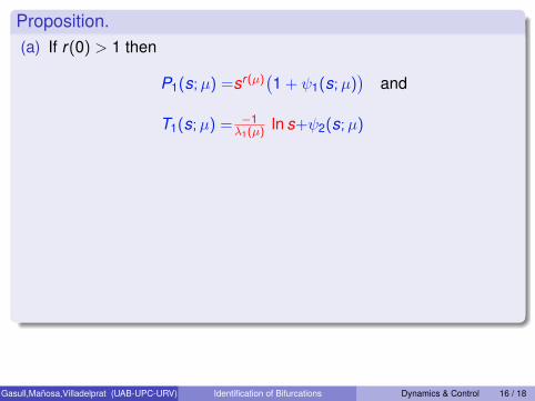
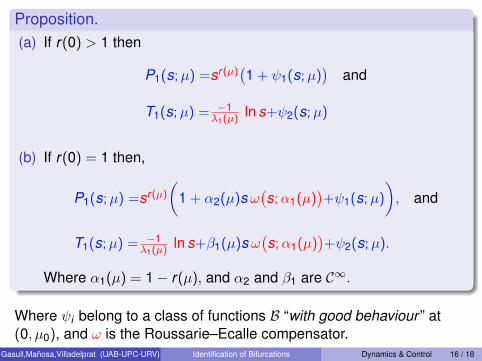
Proposition.(a) If r(0) > 1 then
P1(s;µ) =sr(µ)(1 + ψ1(s;µ)
)and
T1(s;µ) = −1λ1(µ) ln s+ψ2(s;µ)
(b) If r(0) = 1 then,
P1(s;µ) =sr(µ)
(1 + α2(µ)s ω
(s;α1(µ)
)+ψ1(s;µ)
), and
T1(s;µ) = −1λ1(µ) ln s+β1(µ)s ω
(s;α1(µ)
)+ψ2(s;µ).
Where α1(µ) = 1− r(µ), and α2 and β1 are C∞.
Where ψi belong to a class of functions B “with good behaviour ” at(0, µ0), and ω is the Roussarie–Ecalle compensator.
Gasull,Manosa,Villadelprat (UAB-UPC-URV) Identification of Bifurcations Dynamics & Control 16 / 18
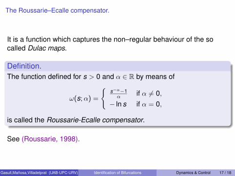
The Roussarie–Ecalle compensator.
It is a function which captures the non–regular behaviour of the socalled Dulac maps.
Definition.The function defined for s > 0 and α ∈ R by means of
ω(s;α) =
{s−α−1α if α 6= 0,
− ln s if α = 0,
is called the Roussarie-Ecalle compensator.
See (Roussarie, 1998).
Gasull,Manosa,Villadelprat (UAB-UPC-URV) Identification of Bifurcations Dynamics & Control 17 / 18
References• Andronov, Leontovich, Gordon, Maier, Theory of bifurcation of dynamic systems on aplane, John Wiley & Sons, New York, 1973.
• Broer, Roussarie, Simo, Invariant circles in the Bogdanov–Takens bifurcation fordiffeomorphisms, Ergodic Th. Dynam. Sys. 16 (1996), 1147–1172.
• Roussarie, Bifurcations of planar vector fields and Hilbert’s sixteenth problem, Progr.Math. 164, Birkhauser. Basel, 1998.
• Sotomayor, Generic one parameter families of vector fields on two dimensionalmanifolds. Publ. Math. IHES, 43 (1974), 5–46.
• Ye et al. Theory of limit cycles, Translations of Math. Monographs 66, AmericanMathematical Society, Providence, RI, 1986.
• The picture in Slide 4 comes from Edgerton Simulating in vivo-like Synaptic InputPatterns in Multicompartmental Models.http://www.brains-minds-media.org/archive/225
THANK YOU!Gasull,Manosa,Villadelprat (UAB-UPC-URV) Identification of Bifurcations Dynamics & Control 18 / 18