IMPERIAL COLLEGE OF SCIENCE AND TECHNOLOGY (University of London) IDENTIFICATION OF STRUCTURAL DYNAMIC CHARACTERISTICS bY Jimin He A thesis submitted to the University of London for the degree of Doctor of Philosophy, and for the Diploma of Imperial College. Department of Mechanical Engineering Imperial College, LONDON SW7 October 1987
Transcript
IMPERIAL COLLEGE OF SCIENCE AND TECHNOLOGY
(University of London)
IDENTIFICATION OF STRUCTURAL
DYNAMIC CHARACTERISTICS
bYJimin He
A thesis submitted to the University of London for the degree of
Doctor of Philosophy, and for the Diploma of Imperial College.
Department of Mechanical Engineering
Imperial College, LONDON SW7
October 1987
1__ __
ABSTRACT
Modal analysis is a rapidly growing field in vibration research. It has been used
effectively in the identification of structural dynamic characteristics and has become a
flourishing area of vibration research. There are some aspects of the modal analysis
method which hinder the application of the method to practical cases. Among them are
analytical model correction, damping properties investigation and nonlinearity study. This
thesis seeks to present the newest development on these aspects.
The dynamic characteristics of a vibrating structure are usually predicted by analytical
techniques such as the Finite Element (FE) method. It is believed that errors in the
analytical model are inevitable, while the modal data extracted from measurement are
usually accepted to be correct, albeit incomplete. Hence, the correlation of an FE model
and corresponding measured data becomes a very important process for structural
vibration research. In this thesis, a new technique is developed to locate the area(s) in an
analytical model where the errors are concentrated by using the incomplete modal data
obtained from tests. An iteration process is introduced for the correction of the analytical
model after the errors are localized and the feasibility of these new techniques is assessed
by both theoretical and practical cases.
Associated with the correction of analytical models, this thesis also investigates the
damping properties of a vibrating structure. It is believed that the most significant
damping often comes from the joints between the various components of a structure and a
method is proposed to locate the spatial damping elements from measurements on the
structure. It is also shown that the located damping could then be quantified using the
iteration process.
Nonlinearity is encountered in many practical structures. However, currently available
means for studying this effect are not fully developed. This thesis describes an
advantageous method, based upon a new understanding of the FRF data measured on a
nonlinear system, to identify more conclusively the nonlinearity and to offer much better f
chance for its quantification. This method has been shown to be effective and convenient
in application and could be very useful for further investigation such as modelling the
nonlinearity and/or predicting the vibration response of the nonlinear system.
. /
2-- __
ACKNOWLEDGEMENT
The author is most grateful to his supervisor Professor D J Ewins for his
continuous help and guidance throughout the duration of this research,
and for his sustained advice in the preparation of the manuscript.
Very special thanks are due to Mr D Robb in the Modal Testing Unit who
was most helpful to the author in computing and conducting experiments.
Thanks are also due to Dr P Cawley, Dr C F Beards and Dr M lmregun in
the Dynamics Section for their useful discussions and help.
Finally, the author is indebted to the Government of the People’s Republic
of China for providing the financial support.
L
3-- em
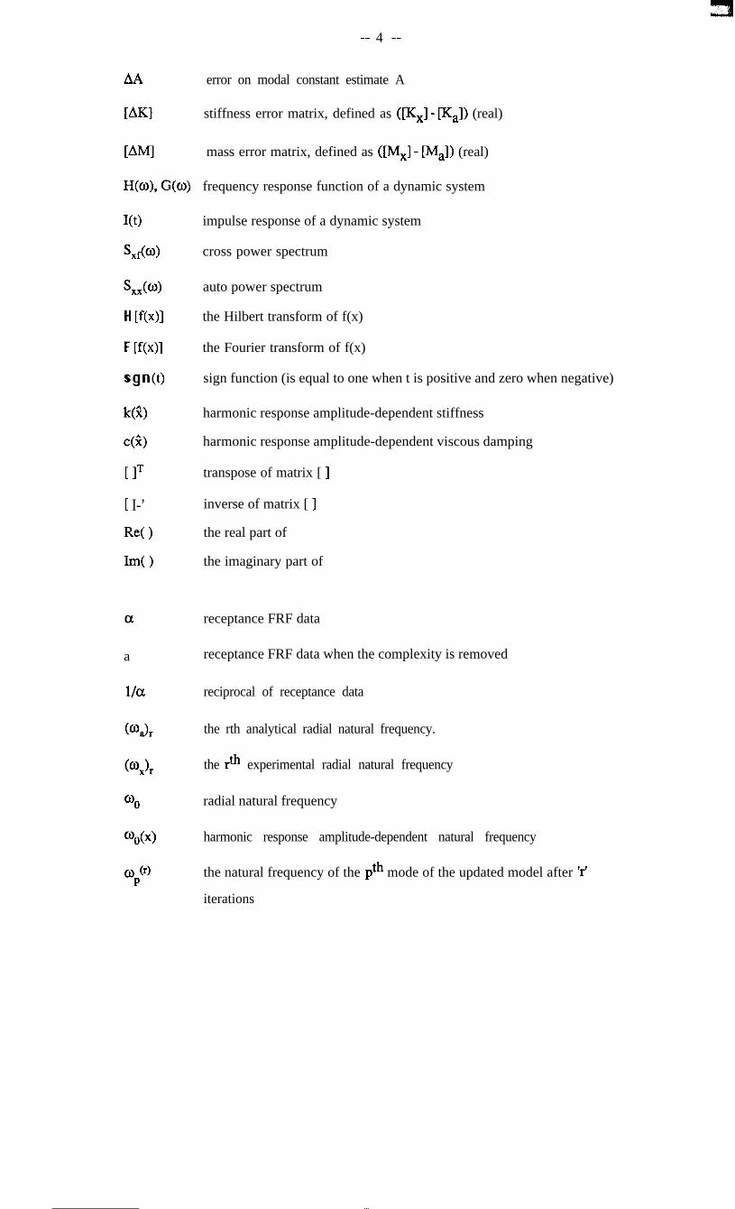
NOMENCLATURE
a
A
Cr
d
i
kij
m
n
N
X
?k
[Cl
[AK,1
WI
[II
RI
wa]R
V&l
W
i”a]R
Wil
subscript for analytical model
modal constant
modal constant of the rth mode
Euclidian norm
imaginary unit
the ‘ij’ element in stiffness matrix
number of measured vibration modes
number of coordinates employed the experimental model
number of coordinates employed by the analytical model
subscript for experimental model
response amplitude of a nonlinear system
symmetric viscous damping matrix (real)
stiffness error matrix, defined as ([KC] - [K,]) (complex)
Table 4-3Natural fkquencies and damping loss factors for Case D3
-
-- 106 --
RealWa)
0
63
Viscous damping case
Real(l/a)
4 co2 0
Hysteretic damping case
Figure 4- 1 Reciprocal of receptance data of one vibration mode with viscous or hysteretic damping
c
-- 107 --
Im I Im
Re
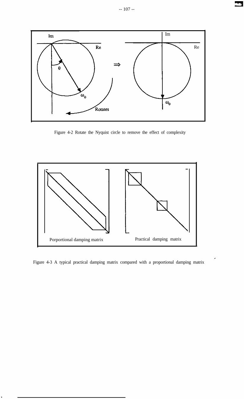
Figure 4-2 Rotate the Nyquist circle to remove the effect of complexity
.
Porportional damping matrix
L
Practical damping matrix
Figure 4-3 A typical practical damping matrix compared with a proportional damping matrix *
.
-- 108 --
1 Incomplete ComDlex 1 I Complete ti
t-i
experimental model analytical model
NJ, [ql W,l, D&J (N$,ls b$
*
Location forFKl and WI
I
Modify analytical model&
construct damping matrix
I
No
Yes I
Yes No
accurate [H]a&
Improvedanalyticalmodel
Iterationfailed
Figure 4-4 Iteration process to estimate [HJ and to improve [K,]
c
_ _. . _. -- _.
\
i-1xl II
L-
cx3 X
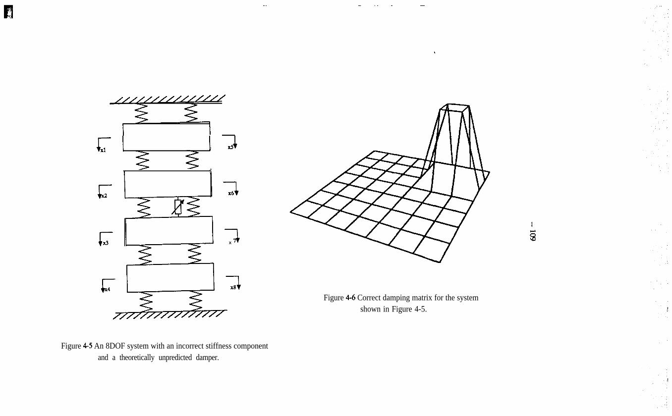
Figure 4-5 An 8DOF system with an incorrect stiffness componentand a theoretically unpredicted damper.
Figure 4-6 Correct damping matrix for the systemshown in Figure 4-5.
mode 1 only mode 2 only
mode 3 only mode 4 only
Figure 4-7 Graphical presentations of the location results for Case Dlusing equation (4-16) with modes from 1 to 4 individually.
Figure 4-8 Graphical presentations of the location results for Case D2 usingequation (4-16) with modes from 1 to 4 individually.Left-hand side columr\: location of stiffness errors.Rm location of damping elements.
-- 112 --
a..w
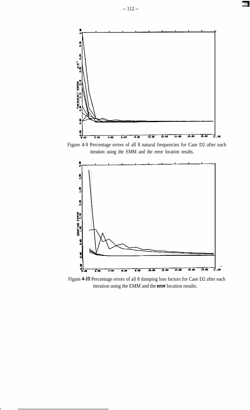
Figure 4-9 Percentage errors of all 8 natural frequencies for Case D2 after eachiteration using the EMM and the error location results.
-4-
a.4
.w
Figure 4-10 Percentage errors of all 8 damping loss factors for Case D2 after eachiteration using the EMM and the error location results.
-- 113 --#I6 I I I 1 1 I I I ‘
SId
?2d
d-00 I .oo 0.00 al.00 lb.00 lb.00 li.00~ lb.00 lb.00 I
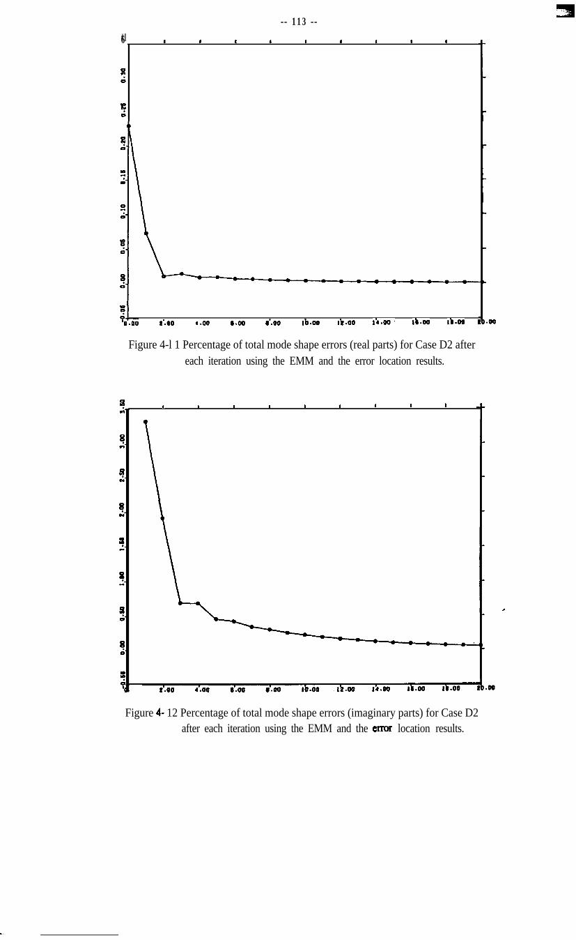
Figure 4-l 1 Percentage of total mode shape errors (real parts) for Case D2 aftereach iteration using the EMM and the error location results.
I I I I I I I I I
,W
Figure 4- 12 Percentage of total mode shape errors (imaginary parts) for Case D2after each iteration using the EMM and the enw location results.
-- 114 --
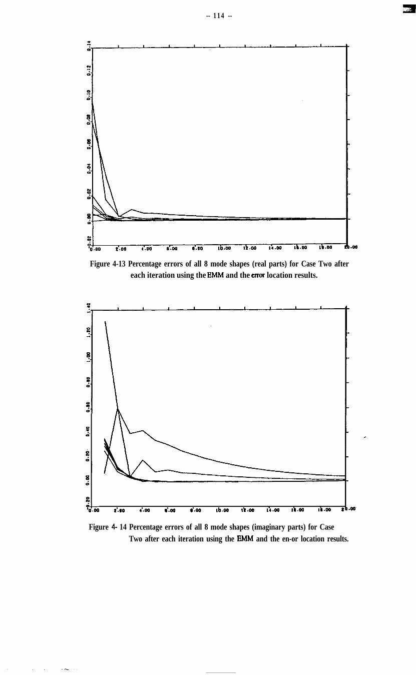
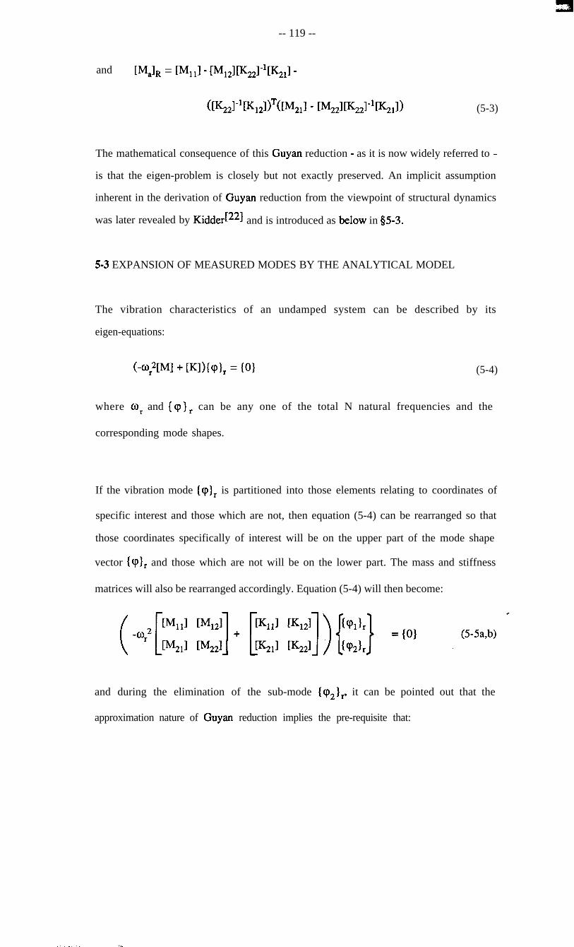
Figure 4-13 Percentage errors of all 8 mode shapes (real parts) for Case Two aftereach iteration using the EMM and the error location results.
Natural frequencies and damping loss factors of the 21 DOF system
-- 130 --
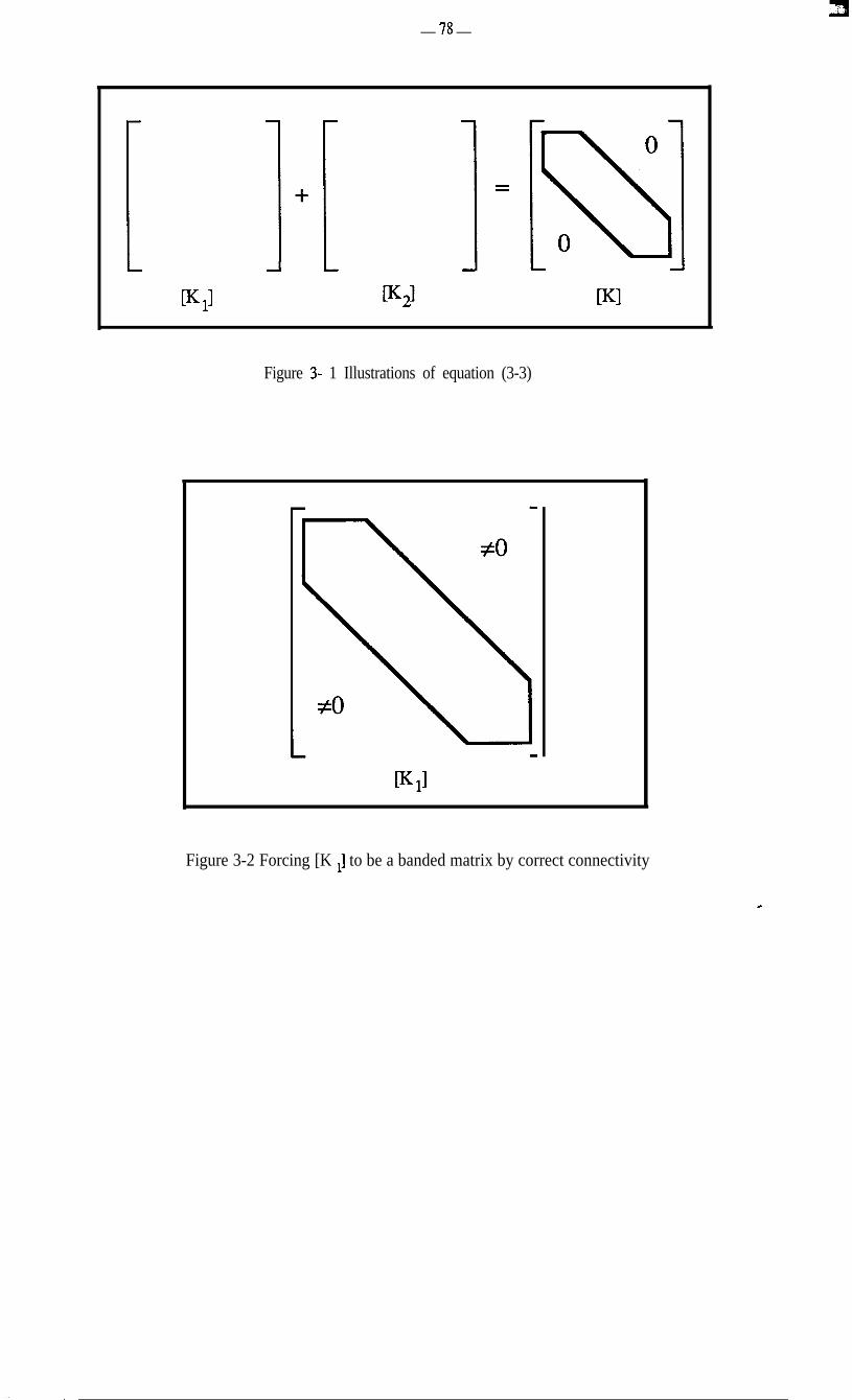
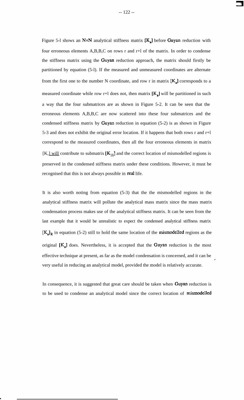
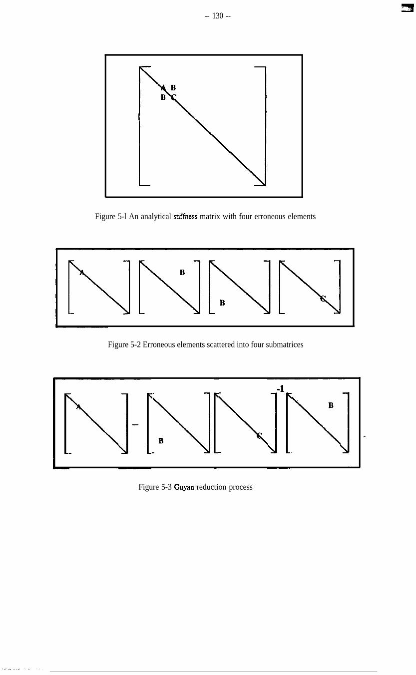
Figure 5-l An analytical stiffness matrix with four erroneous elements
Figure 5-2 Erroneous elements scattered into four submatrices
_\\]
B_
.
\
B
\.
Figure 5-3 Guyan reduction process
c
-- 131 --
0 II 0 0 ?1 0
i j j+l i+l
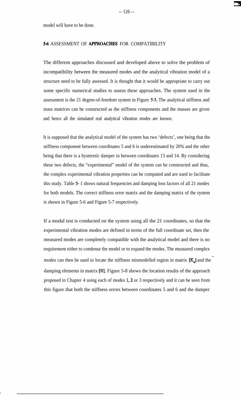
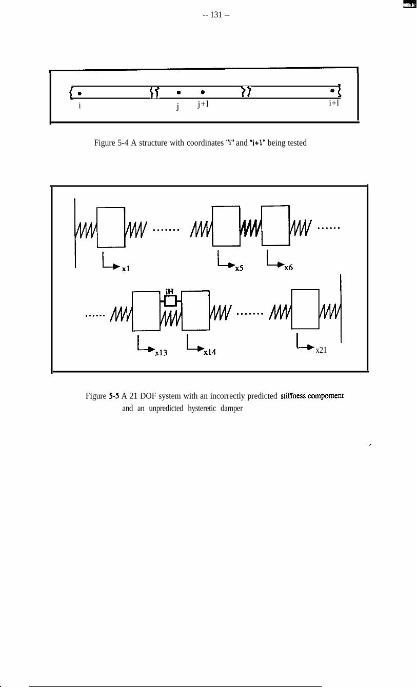
Figure 5-4 A structure with coordinates ‘5” and “i+l” being tested
. . . . . . . . . . . . .
L,, L,,
. . . . . . . . . . . . .
Ll3 Ll4 Lx21
Figure 5-5 A 21 DOF system with an incorrectly predicted stiffness compomentand an unpredicted hysteretic damper
c
-- 132 --
Figure 5-6 Correct stiffness error matrix [AK] for the system shown in Figure 5-5.
Figure 5-7 Correct damping matrix [HJ for the system shown in Figure 5-5.
L ,
mode 1 only
mode 2 only
mode 3 only
Figure 5-8 Location of stiffness errors and damping elements in the system shownin Figure 5-5 using experimental modes 1,2 and 3 respectively.
Left-hand side column: location of stiffness errors.Bight-hand side column: location of damping elements.
Expanded mode 2 only
Expanded mode 3 only
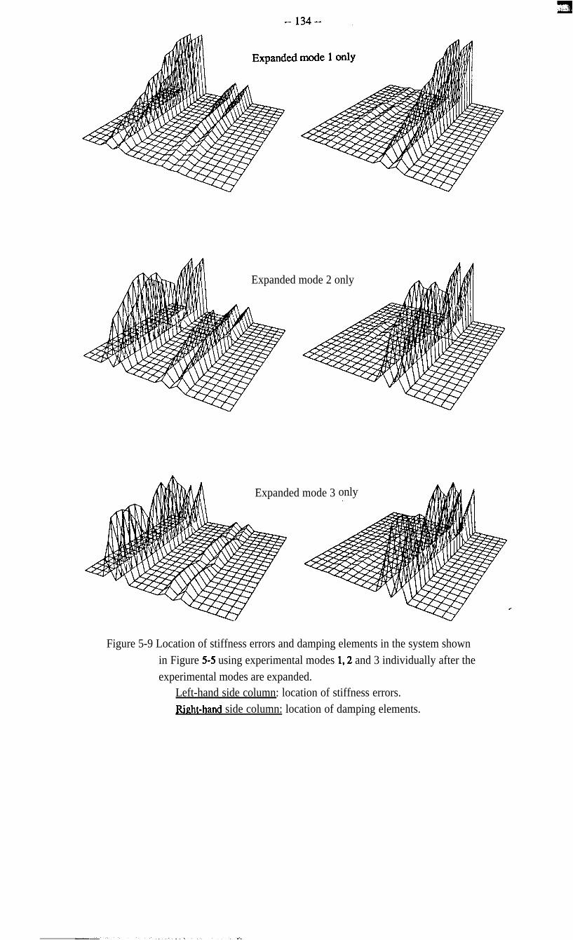
Figure 5-9 Location of stiffness errors and damping elements in the system shownin Figure 5-5 using experimental modes 1,2 and 3 individually after theexperimental modes are expanded.
Left-hand side column: location of stiffness errors.fight-hand side column: location of damping elements.
c
-- 136 --
CHAPTER 6
APPLICATION OF MODELLING ERROR LOCATION
TO A PRACTICAL STRUCTURE
6-l INTRODUCI’ION
In the early parts of this thesis, it has been noted that the dynamic characteristics of a
structure are widely investigated by two approaches, these being theoretical modelling and
experimental testing. It has also been stressed that the dynamic characteristics can be fully
and correctly understood only if these two approaches are made in parallel, in order to
offset the weaknesses of both. The strong demand in vibration research and engineering
practice to use the measured vibration modes in order to improve the analytical model of a
vibration structure has also been identified.
Several methods which currently facilitate the model improvement process have been
reviewed and studied in Chapter 2. It is found that the main drawback of these methods is
that the resultant improved analytical stiffness or mass matrix does not adequately
represent the structure modelled analytically since these methods attempt to modify the
whole analytical model and end up with an ‘improved’ model which violates the actual
connectivity of the structure. The vibration characteristics deduced by a thus-improved
model will therefore not be correct and even the iteration process suggested in Chapter 2
cannot overcome this drawback and achieve the correct model. In addition, we lack an
appropriate method to investigate the damping properties of vibrating structures and the ’
proportional damping assumption is believed to be impractical in real Iife applications.
Since it is realized that, for most vibrating structures, the modehing errors inherent in their
analytical models are usually local - due to the sophisticated modelling techniques - and
L I
-- 137 --
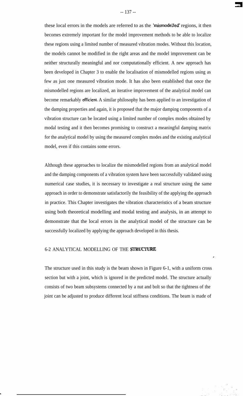
these local errors in the models are referred to as the k&modelled’ regions, it then
becomes extremely important for the model improvement methods to be able to localize
these regions using a limited number of measured vibration modes. Without this location,
the models cannot be modified in the right areas and the model improvement can be
neither structurally meaningful and nor computationally efficient. A new approach has
been developed in Chapter 3 to enable the localisation of mismodelled regions using as
few as just one measured vibration mode. It has also been established that once the
mismodelled regions are localized, an iterative improvement of the analytical model can
become remarkably effkient. A similar philosophy has been applied to an investigation of
the damping properties and again, it is proposed that the major damping components of a
vibration structure can be located using a limited number of complex modes obtained by
modal testing and it then becomes promising to construct a meaningful damping matrix
for the analytical model by using the measured complex modes and the existing analytical
model, even if this contains some errors.
Although these approaches to localize the mismodelled regions from an analytical model
and the damping components of a vibration system have been successfully validated using
numerical case studies, it is necessary to investigate a real structure using the same
approach in order to demonstrate satisfactorily the feasibility of the applying the approach
in practice. This Chapter investigates the vibration characteristics of a beam structure
using both theoretical modelling and modal testing and analysis, in an attempt to
demonstrate that the local errors in the analytical model of the structure can be
successfully localized by applying the approach developed in this thesis.
6-2 ANALYTICAL MODELLING OF THE STRUCIUREc
The structure used in this study is the beam shown in Figure 6-1, with a uniform cross
section but with a joint, which is ignored in the predicted model. The structure actually
consists of two beam subsystems connected by a nut and bolt so that the tightness of the
joint can be adjusted to produce different local stiffness conditions. The beam is made of
-- 138 --
steel and is about 2m long with cross section of 25mm x 18Smrn.
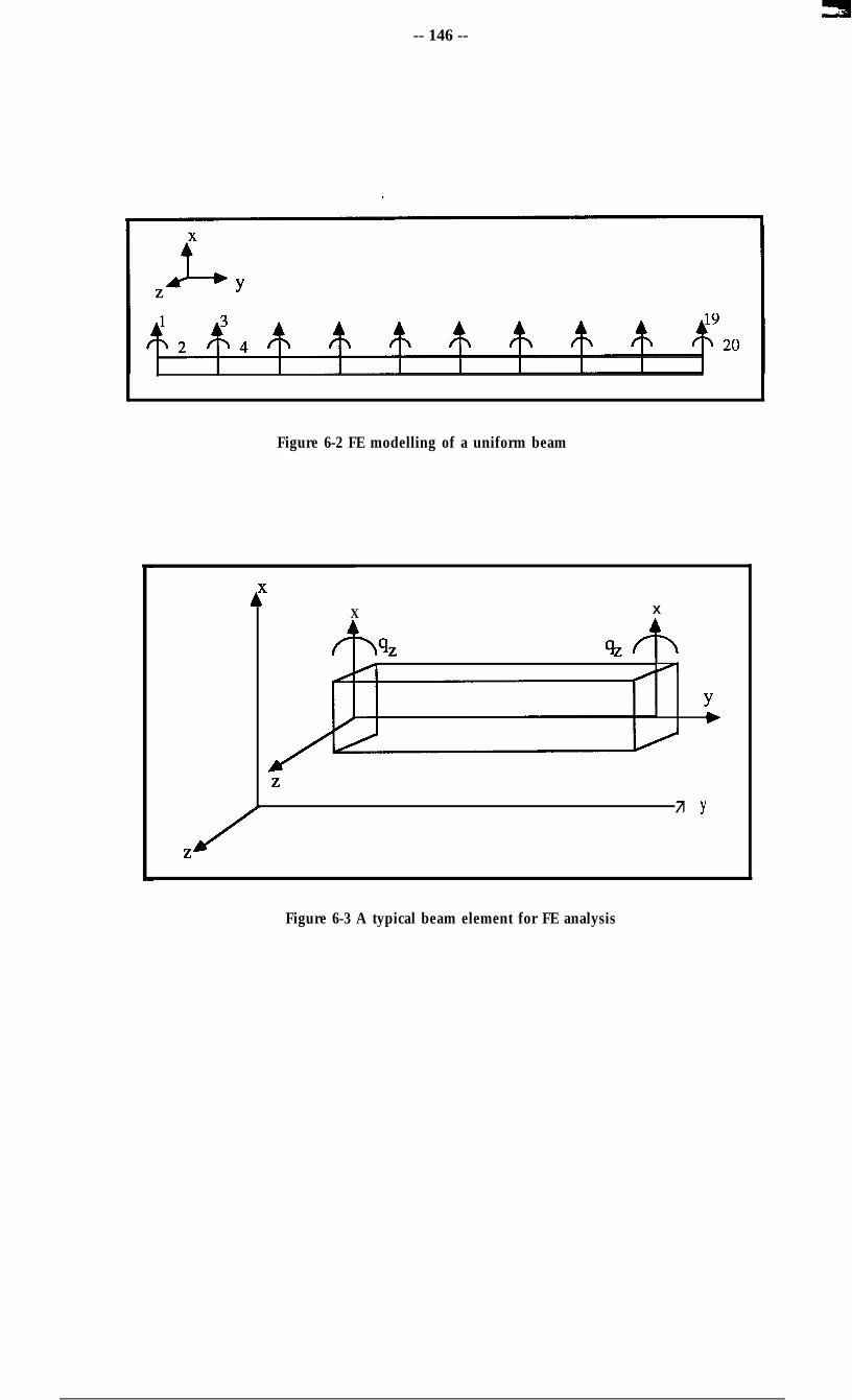
A finite element analysis is carried out for this beam structure, ignoring the joint, so that
the structure is regarded as a uniform beam shown in Figure 6-2. This is divided into 9
equal length beam elements and, taking into account both the translational and the
rotational displacements in directions x and 8, as shown in Figure 6-3, mass and stiffness
matrices can be derived for the beam element (Appendix 3). Global analytical mass and
stiffness matrices which form the analytical model of the structure can then be
constructed. The analytical mass and stiffness matrices thus obtained have a dimension of
20x20. It is believed that the analytical mass matrix of this structure is reasonably accurate
since the structure does not have any sudden changes of section while the analytical
stiffness matrix obviously does not represent the true stiffness distribution because it does
not take account of the local stiffness change near the joint
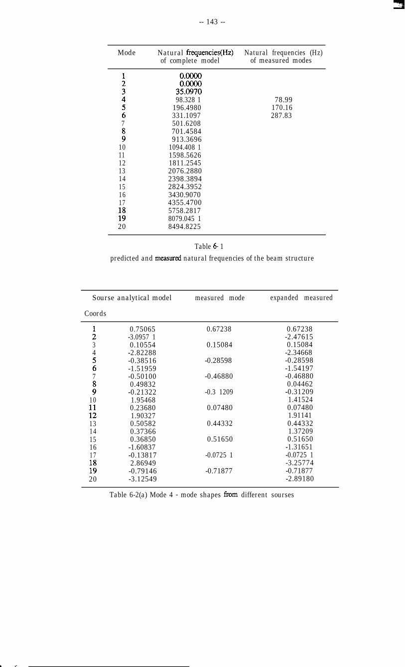
The analytical vibration modes of the structure are obtained by the eigen-solution of the
analytical model. Table 6-l shows all the 20 natural frequencies of the analytical modes,
including two zero natural frequencies for the rigid body modes. The left hand column in
Table 6-2 shows the mode shape vectors of 4,5, and 6 analytical vibration modes derived
by the analytical model. It can be seen that the analytical vibration modes are defined in
both the rotational and translational coordinates and these are alternately positioned in the
mode shape vectors. Specifically, those odd-numbered coordinates are translational
coordinates and the even-numbered rotational ones.
6-3 MODAL TESTING AND ANALYSIS OF THE BEAM STRUCTURE AND THE 4
COMPARISON OF lTS MODAL MODEL AND FE MODEL
The modal testing was carried out with the structure supported by two soft strings at its
ends, simulating a free-free boundary condition, as shown in Figure 6-4. The testing was
-- 139 --
carried out at ten translational coordinates in the x direction, as indicated in the Figure 6-4.
As suggested by the modal testing theory, one column of the FRF matrix of a system is
theoretically sufficient to extract the modal model of the system, provided the excitation
point is selected such that all the interesting vibration modes can be excited. After careful
examination, it was decided that structure was to be excited at point 3 (coordinate 5)
where all the interested modes show up. Equipment set-up is also displayed in Figure
6-4. The frequency response analyser used in this test was Solartron 1250 analyser which
facilitates standard discrete sinusoidal signal. The Modal Testing software ‘POLAR’ is
used for the data acquisition and software ‘MODENT’ used for the analysis. Both
programs are developed in the Modal Testing Unit in this department and, in this study,
they were run on an HP computer.
A fast sinusoidal excitation sweep was used first in the frequency range of interest in
order to identify the vibration modes. Then, a roomed sinusoidal excitation was used in
the test and the acceleration response at each coordinate was recorded while the excitation
force is applied on point 3, so that the frequency response function (FRF) could be
obtained from the frequency response analyser. Figure 6-5 shows a typical frequency
response function obtained in measurement. Its counterpart in the Argand plane is shown
in Figure 6-6. The data exhibit quite clearly-defined modal properties for the structure
within the measured frequency range.
In this study, only three vibration modes were measured and analysed for the purpose of
stiffness error location. The measured natural frequencies of these three modes are shown
in the right hand column of Table 6-l. Table 6-2 compares these three measured vibration
modes with those predicted by the analytical model. The difference between the measured
natural frequencies and those predicted analytically, and that between the mode shapes, is *
apparent and is expected to be caused by the fact that the analytical model does not
correctly model the true stiffness distribution of the beam structure because of the joint.
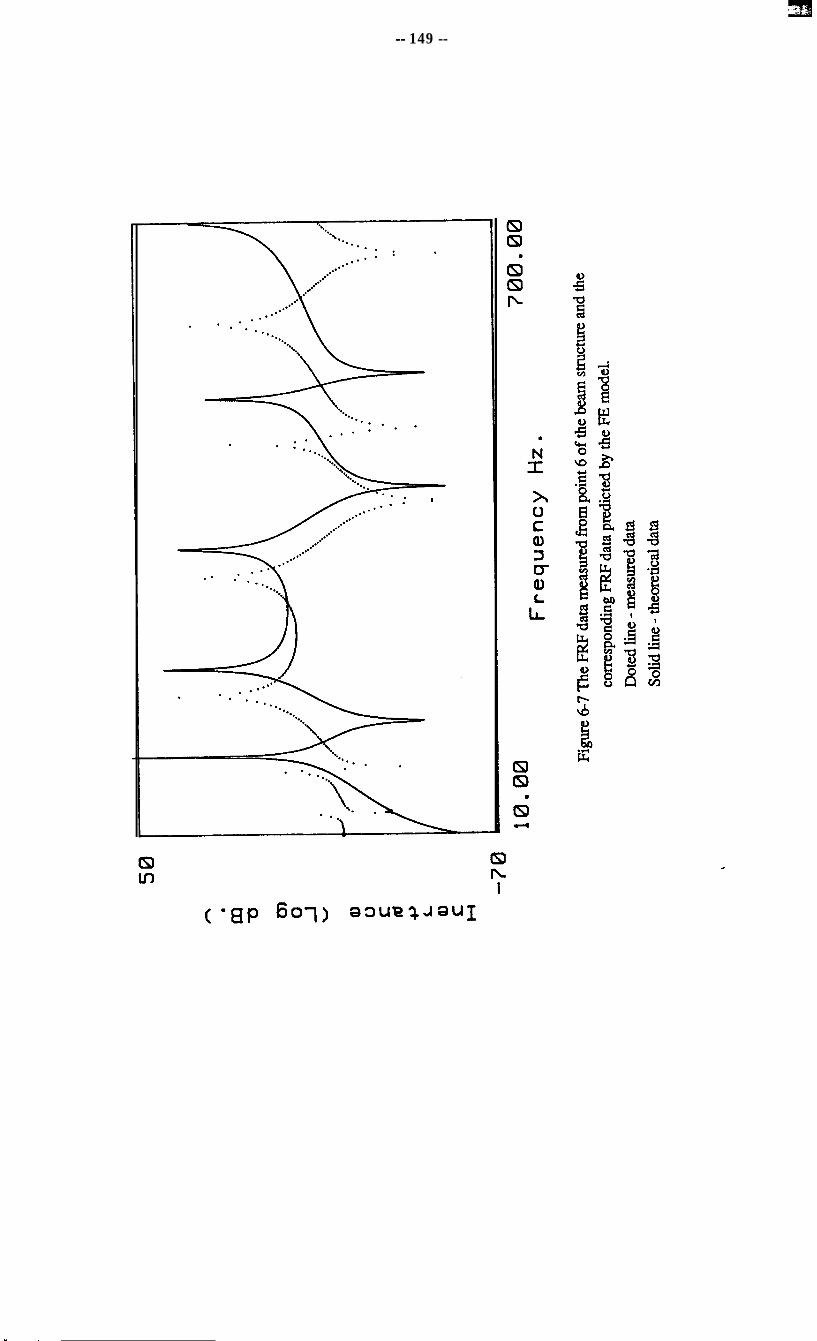
Figure 6-7 shows the FRF data measured from point 6 within a certain frequency range
and the corresponding FRF data predicted by the FE model. It can be clearly seen that the
-- 140 --
vibration modes predicted theoretically exhibit different dynamic characteristics of the
structure from the vibration modes obtained experimentally. Again, this is due to the
different stiffness conditions which apply to the analytical and experimental configuration.
6-4 LOCATION OF THE MISMODELLED REGION IN ANALYTICAL
STIFFNESS MATRIX USING MEASURED VIBRATION MODE
641 Expansion of Measured Vibration Modes
In order to localize the modelling errors in the analytical stiffness matrix, the
incompatibility between the analytical model and the measured vibration modes in terms
of the coordinates specified has to be overcome first. As proposed in Chapter 5, the three
measured vibration modes are expanded to include those rotational coordinates which are
not measured, using the analytical mass and stiffness matrices. The three thus-expanded
measured mode shapes (rearranged to the original coordinate order as the analytical mode
shapes adopt) are listed in Table 6-2, together with the corresponding analytical mode
shapes for the sake of easy comparison. It can be seen fi-om Table 6-2 that the measured
translational coordinates in the expanded mode shapes are unchanged while the rotational
coordinates in the expanded mode shapes are effectively interpolated into the mode shapes
by the analytical model. In addition, the measured natural frequencies are not changed
during this mode shape expansion procedure.
6-4-2 Location of Mismodelled Region in the Analytical Stiffness Matrix
The three expanded measured vibration modes are then used to locate the errors in the
analytical stiffness matrix. Figure 6-8 shows the results of locating the errors using each *
expanded measured vibration modes individually and then using three measured modes
together, and this figure indicates that each result consistently points to the same region in
the analytical stiffness matrix where stiffness modelling errors exist. Namely, the errors
are confined in those elements between rows 13 and 17, corresponding to the testing
-- 141 --
points between 7 and 9.
To interpret the results shown in Figure 6-8, it has to be noted that the unpredicted joint in
the beam structure (ignored in the analysis) is situated between the test points 7 and 8 and,
according to the explanation of Chapter 5, the stiffness modelling errors should be located
between test points 7 and 8 (which correspond to the global coordinates between 13 and
16). However, the results in Figure 6-8 for using each expanded measured vibration
consistently indicate the stiffness modelling errors between testing points 7 and 9, which
relate to global coordinates 13 to 18. This is eventually answered by inspection of the
structure. Since the joint which is sited between test points 7 and 8 is close to point 9
side, the significant tightness of the joint eventually affects the stiffness condition between
points 8 and 9, so that the modelling errors are indicated not only between points 7 and 9,
but also between 8 and 9.
To be fully convinced of the location obtained above using the measured vibration modes,
one extreme condition is now considered. It is understood that the measured modal data
values could possibly vary due to the testing conditions, numerical calculation errors etc.
In order to simulate the possibility of different test results, and the consequence of that on
the location of the stiffness modelling errors in this study, all the measured natural
frequencies and mode shapes of the three modes are perturbed by five percent random
errors and these revised measured modes are then used, as before for the unperturbed
modes, to locate the errors in the analytical stiffness matrix. Figure 6-9 shows the results
using the revised modes 4, 5 and 6 individually and it can be seen that just the same
modelling error location is obtained, as before. This shows that the correct modelling
error location can be achieved even the measured data have some realistic errors.c
6-5 CONCLUSIONS
A practical application of the approach proposed in the early part of this thesis to locate the
r&modelled region in the analytical model of a structure has been carried out. The
-- 142 --
primary purpose of this part of the study is to assess the practical feasibility of the
approaches proposed so far in this thesis in locating the modelling errors which exist in
the analytical model of a structure using just a few number of the measured vibration
modes.
The structure upon which the investigation was performed is a beam structure with an
analytically ignored joint which causes the modelling errors in the analytical stiffness
matrix of the structure. The analytical model is obtained assuming the structure to be a
uniform beam and the analytical mass and stiffness matrices can be derived by Finite
Element modelling. The stiffness matrix thus derived contains errors relating to the local
area where the joint exists while the mass matrix is believed to be acceptably accurate
since there is no sudden mass change on the structure.
Modal testing was carried out using the ten translational coordinates of the structure only,
as the remaining rotational coordinates defined by the analytical model are technically
difficult to test. Only three vibration modes were identified experimentally.
Since an incompatibility exists between the measured vibration modes and the analytical
model, the three measured vibration modes were expanded using the analytical mass and
stiffness matrices, as suggested in Chapter 5. These three expanded vibration modes were
then used to locate the modelling errors assumed to be present in the analytical stiffness
matrix.
The results of using the expanded vibration modes individually to locate modelling errors
in the analytical stiffness matrix have consistently pinpointed the correct region in the
*matrix which relates the local area in the structure where the unpredicted joint is situated.
-- 143 --
Mode Natural frequencies(Hz) Natural frequencies (Hz)of complete model of measured modes
Table 6-2(c) Mode 6 - mode shapes from different sourses
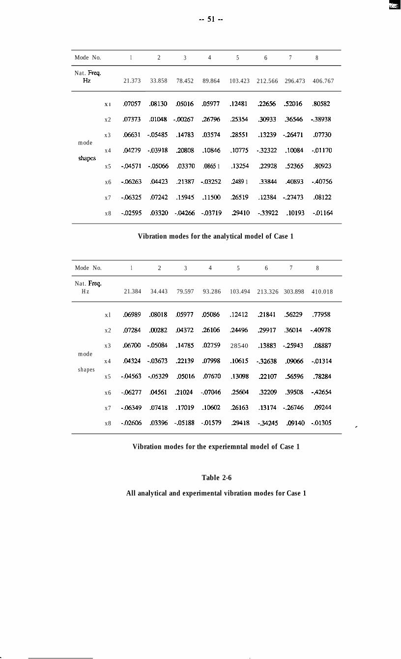
Table 6-2Mode shapes for vibration modes 4,5,6 of the beam structure
I I I II I
Figure 6-l a uniform with an unpredicted joint
-- 146 --
Figure 6-2 FE modelling of a uniform beam
X X
I
Yb
Z
ä Y
Z
Figure 6-3 A typical beam element for FE analysis
Test point 1
Coord. No.( 1)
0 0 0 0 0 l 0
2 3 4 5 6 7 8 9 10
(3) (5) (7) (9) (11) (13) (15) (17) (19)
Beam structureA
Shaker 4
Charge amplifier
Power amplifier cl Sine signal geberator
Frequency response functionb
for modal analysis
Figure 6-4 Modal testing of the beam structure
-- 148 --
5 0
1 2 . 0 0 F r e q u e n c y H z . 6 9 8 . 0 0
Figure 6-5 A typical frequency response function obtained from modal testof the beam structure shown in Figure 6-4.
x
x x
X xX
XX _ _
XX
X
X
XXXX*cx x
X%
iit-- -7
X
x
XXXXX
,
fstrr-~
X
* x
* x
xxXX
,u2(N
REAL + ve.>
Figure 6-6 The FRF in Figure 6-5 is presented in the Argand plane.
-- 149 --
c
I ,
Expanded mode 4 only Expanded mode 5 only
Expanded mode 6 only A Expanded modes 4,5 and 6
Figure 6-8 Location of stifTncss enors for the beam structure shown in Figure 6-4using experimental modes 4.5 and 6 individually and then together
\ after the experimental modes arc expanded.
Expanded mode 4 only
Expanded mode 6 only Expanded modes 4,5 and 6
Figure 6-9 Location of stiffness errors for the beam structure shown in Figure 6-4using experimental modes 4,5 and 6 individually and then together afterthe experimental modes are expanded and 5% artificial random errors areadded into the natural frequencies and mode shapes.
c
-- 153 --
CHAPTER 7
MEASUREMENT OF NONLINEARITY
7-1INTRODUCFION
In the previous Chapters, we have covered one of the most important and demanding
topics in the recent vibration research: that of correlating the analytical model of a dynamic
structure and its measured vibration modes so that an improved model can be obtained.
This is expected to combine the advantages of the two widely used approaches (analytical
modelling and experimental testing) in order to understand better the dynamic
characteristics of the structure under investigation. The damping properties of a structure
have also been studied.
In those previous studies, it is assumed that linearity exists for the structures modelled
analytically and tested but it is realised that all real vibrating structures are nonlinear to
some degree. However, many of them may be nonlinear to a tolerable extent so that they
can still be investigated using the theory for linear structures. For those structures known
or suspected to be noticeably nonlinear in their vibration behaviour, the linear assumption
fails to be applicable and special analysis is needed to investigate the nonlinearity.
Generally, it can be said that nonlinearity is similar to the modelling errors and damping
properties discussed earlier in the sense that it also cannot be predicted analytically and
can only be identified by experimental measurement.c
The study of nonlinearity is very complicated. This results from the fact that the
superposition principles whereby the response of a system to different excitations can be
added linearly is not valid in the case of nonlinear systems. As a consequence, the
dynamic characteristics of nonlinear structures become excitation-dependent and much
-- 154 --
less predictable. Since the nonlinearity encountered in vibrating structures is often difficult
to identify, and even more difficult to quantify, they are in many practical cases significant
to the vibration behaviour of the structure, and the requirement for special investigation
methods is clear.
It is noted that theoretical methods have been developed extensively for those nonlinear
systems whose equations of motion can be expressed analytically. The fundamental point
of the analysis can be classified briefly as linearising either the parameters of a nonlinear
system or its vibration response. There are currently quite a number of methods which are
available to examine the vibration behaviour of a nonlinear system analytically. For
example, the Small Oscillation Method is an approach which replaces the nonlinear term
in the differential equations of a nonlinear system by its Taylor series with respect to
displacement and velocity and considers only the fast two terms, thereby extracting a
linear system which will exhibit a response like the nonlinear system; The Quasi-harmonic
Method[54] aims at deriving a periodic solution for a nonlinear system in the form of a
power series in E (a parameter which indicates the perturbations of the system and is
considered to be very small). Thus, a time-dependent solution which does not differ
appreciably from the solution of the corresponding linear equation can be sought. The
Method of Krylov and Bogolyubov supposes that the solution to the equation of a
nonlinear vibrating system is still in the same form as that of its linear counterpart, except
that the amplitude and phase are slightly varying with time and, as a consequence, the
approximate solution of the nonlinear system is a periodic function of both the amplitude
and phase angle, as weIl as time. An equivalent natural frequency and damping coefftcient
of the nonlinear system subjected to an external excitation can then be obtained as
functions of the response amplitudef 551. Iwan’s New Linearisation Method[561 is a
generalisation of the method of equivalent linearisation. It introduces a weighting function c
into the averaging integrals used in the equivalent linearisation method and suggests that a
nonlinear second order system can be replaced by a linear system in such a way that an
average of the difference between the two systems is minimized. It also shows that the
replacement is unique and can be accomplished in a straightforward manner.
. .
-- 155 --
Apart from the methods summarized above for general nonlinear cases, analysis could be
further developed to cope with systems having known types of nonlinearity. For instance,
such studies can be traced back to dates long before the computer was available[57] or,
they can be found from time to time in recent ~terature[~*l~[~~l.
Although many types of nonlinearity have been studied extensively, based on
mathematics and analysis used in control engineering, the theory is often not directly
applicable to experimental modal analysis of real structures because of the absence of
explicit equations of motion for practical vibration situations. The major difficulty in these
situations is the detection and identification of the nonlinearity when what is available is
the response of a nonlinear structure to excitation by external forces rather than an explicit
analytical description. Nevertheless, the theoretical study provides many specific and
frequently encountered types of nonlinearity with characteristic response patterns which,
in turn, provide a helpful reference in practical modal analysis.
7-2 EXCITATION TECHNIQUES
It is customary to assume that for linear structures, the dynamic characteristics will not
vary according to the choice of the excitation technique used to measure them. However,
the effects of most kinds of nonlinearity encountered in structural dynamics are generally
found to vary with the external excitation and hence the fust problem of a nonlinearity
investigation will necessarily be to decide a proper means of excitation so that the
nonlinearity can be easily exposed and then identified. There are currently mainly three
types of excitation method widely used in vibration study practice and each of them is
discussed below.c
7-2-l Sinusoidal Excitation
Sinusoidal excitation is the traditional excitation technique in vibration testing and also in
-- 156 --
recent modal testing practice. Although many other techniques such as random, transient,
periodic and pseudo-random excitations etc have been developed, sinusoidal excitation is
still commonly applied in practice because of its uniqueness and precision. The main
advantages of this excitation can be summarised as:
(a) sinusoidal excitation can accurately control the input signal level and hence it
enables a high input force to be fed into the structure. This is especially significant
when large structures are tested,
(b) for discrete sinusoidal excitation, the signal-tonoise ratio is generally good as the
energy is concentrated in one frequency band each time and even swept sinusoidal
excitation can normally achieve similar concentrated energy conditions compared
with other excitation methods;
(c) sinusoidal excitation is widely regarded as the best excitation technique for the
identification of nonlinearity in most applications of modal testing and analysis;
(d) when the harmonic distortion effects of nonlinearity are investigated, sinusoidal
excitation is also uniquely required.
It is the item (c) that contributes most to the continued wide application of this traditional
excitation technique. In this study, sinusoidal excitation is employed for each nonlinearity
simulated on an analogue computer in order to facilitate the nonlinearity identification
process.
The main drawback of the sinusoidal excitation technique is that it is relatively slow
compared with many of the other techniques used in practice. The obvious reason is that
the excitation is performed frequency by frequency and, at each step, time is needed for
the system to settle to its steady-state response. However, it is believed that for many
practices of the identification of structural dynamic characteristics, correct measurement *
results often become the primary criterion over time-saving in the test. For instance, when
the modal analysis results are to be used to improve an FE model of the tested structure -
an application which appears to be in great demand in recent years and has been
exhaustively discussed above - a major concern lies on the precision and comprehension
-- 157 --
of the modal analysis results. Consequently, sinusoidal excitaion is preferred in modal
testing in order to provide the post analysis stages with the optimum data.
7-22 Random Excitation
Random excitation attracts analysts and researchers primarily because of its potential time
saving in obtaining frequency response functions of the tested objects. Using this
technique, the system is excited simultaneously at every frequency within the range of
interest. This wide frequency band excitation enables the technique to be much faster than
sinusoidal excitation. Further, the effects of noise can be successfully eliminated by
averaging if the measurement time is long enough.
The derivation of the input and output relationship under random excitation relies on
Fourier transform theory and is based upon Duhamel’s Integral. As the Duhamel’s
Integral presumes a linear system behaviour, it has been suggested in the literature that the
linearity characteristic of the response from the random excitation is automatically
assumed. It will be shown below that this is not true. The actual reason for the inability of
random excitation to expose the nonlinearity from the response is the randomness of the
amplitude and phase of the input force.
In the measurement, spectral estimates for each recorded data block have random
amplitude and random phase. Thus, at each frequency the system can be considered to be
excited by different amplitudes and phases, sample after sample. By considering the effect
of nonlinearity as noise in the response, it can be understood that after the averaging
process the frequency response function obtained from the FFI’ analyser will always
comply with the behaviour of a linear system. It can then be roughly concluded that as far ’
as the identification of nonlinearity is concerned, conventional random excitation and
signal analysis is not a feasible technique in practice.
It should be noted here that the problem of impedance mismatch between the tested
_-
-- 158 --
structure and the shaker always exists and this can result in problem of noise. Usually,
the spectrum of the excitation signal is uniform along the frequency range of
measurement. However, when a mismatch occurs, the spectrum of the excitation force
applied to the structure may be distorted, yielding noise problems. The mismatch problem
is most serious at the resonances of the structure when the response spectrum at the
vicinity of resonance tends to drop because of the low impedance input to the structure,
resulting in a low signal-noise ratio.
Sometimes, when the dynamic modelling of a nonlinear system is of concern rather than
the identification of nonlinearity, the primary interest will be on extracting a linear model
of the system which behaves vibrationally in the frequency range of interest in as similar a
manner as possible to the nonlinear system, regardless what type of nonlinearity the
system possesses, then random excitation could be an effective technique.
7-23 Transient Excitation
Since the Fourier Transform was fust developed in the early nineteenth century, the
theoretical foundation had been provided for transient testing. However, not until digital
computers with FFT capabilities were developed did transient excitation and analysis
become practically feasible and has now received great interest because of the unique
characteristics differing from other excitation techniques.
In transient excitation measurement, the data involved are the time histories of the
excitation force f(t) and of the response x(t). The frequency response function is defined
by the division of the Fourier Transforms of these two time series signals. The
denominator is the Fourier Transform of f(t) whereas the numerator is the Fourier c
Transform of x(t):
H(o) = X(O) /F(W) (7-l)
-- 159 --
The actual computer analysis approach to obtain the frequency response function depends
on the estimates of the auto-spectrum of the force signal and the cross-spectrum of the
force and response. The computation is performed as:
H(o) = X(0) /F(O)
= X(o)F*(o) / F(o)F*(o)
(7-2)
where F*(o) is the complex conjugate of the Fourier Transform F(o) and SJo) is the
cross-spectrum of the force and the response of the system. Therefore, obtaining the
frequency response function in transient testing becomes a matter of spectral analysis.
The form of the forcing function in transient excitation is important. The input forcing
function theoretically suggested for transient excitation is of a pulse type. This is,
unfortunately, mechanically difficult to achieve in practice. Usually, a mechanical impact
is used to generate the required forcing signal. If the impact is well controlled, the forcing
signal would have a comparatively short time duration and contain desirable energy
spectral properties. However, a very short duration of an impact, covering a broad range
of energy distribution in the frequency domain, can be extremely difficult to obtain in
practice. This means that in the frequency domain the input force energy at high
frequencies is not always large enough to excite the system effectively. Hence, care
should be taken when transient excitation is applied to the case where vibration properties
at high frequency are of primary interest. Moreover, it is quite obvious that the excitation
frequency bandwidth cannot be controlled conveniently.
One possible alternative to the mechanical impact forcing signal is an electrical, instead of *
mechanical, impulse which can be applied to the strncture through a conventionally used
shaker. Indeed, this type of electrical pulse test has been adapted. Despite the fact that an
electrically-produced forcing signal has well controlled amplitude, a desired rectangular
c
__ 160 __
shaped pulse signal is still not easy to achieve due to a number of error sources such as
the “digitising error” occurring in the operation of A/D (analogue to digital) conversion.
Besides, the frequency characteristics of a shaker could be a problem and this is perhaps
more important,
Another forcing function referred to as “rapidly swept sinewave” or “chirp”, which is
classified in the transient excitation category, has been employed with success in recent
years[60]. Unlike the discrete sinewave used in sinusoidal excitation, the swept sinewave
here is of constant amplitude and has a sweeping frequency which varies rapidly and
continuously with time and has high cut-off rate at the starting and ending frequencies.
The time duration of the forcing signal can be as short as a few seconds. However, no
evidence has been found to back up the advantage of using such a excitation technique for
the purpose of identifying nonlinearity.
7-2-4 Comments on Different Excitation Techniques
Although there are a number of excitation techniques available nowadays for vibration
testing, the choice for the modal testing of a dynamic structure is by no means easy,
especially when nonlinearity is to be investigated.
Random excitation tends to excite the structure with a random force level and phase at
each frequency and thus the response data from a nonlinear system will behave as if the
system were linear, as the recorded data blocks are averaged. As the contribution of the
nonlinearity to the response differs from noise in that it is a systematic error and cannot be
averaged out, the response data from a nonlinear system will appear to be from a linear
system which is often referred to as a ‘linearised model’ of the nonlinear system, rather +
then the linear part of the nonlinear system. This is illustrated in Figure 7-l. Hence,
random excitation is not applicable for the purpose of the identification of nonlinearity. In
other cases, when the dynamic modelling of a nonlinear system is of interest, rather than
the identification of nonlinearity is sought, the primary concern will be on the extraction
L
-- 161 --
of a linear model of the system which will behave vibrationally in as similar a manner as
possible to the nonlinear system in the frequency range of interest, regardless of what
type of nonlinearity the system possesses, then random excitation could be an efficient
technique.
Transient excitation has noticeable
remarkably fast in performance. It
properties of convenience and simplicity and is
requires less instrumentation (for the case of a
mechanical impact test), facilitating mobile experiments. However, transient excitation
obviously attracts the same argument as random excitation in not being applicable for the
purpose of the detection and identification of nonlinearity. This is mainly because the
force level and phase of each data record is similarly not controllable as for the random
excitation case and, in addition, the frequency range is also difficult to control.
Nevertheless, low coherence often occurs at anti-resonances of the frequency response
function data when the impact test is carried out. This is mainly because of the low
signal/noise ratio at anti-resonances. This characteristic is different from the random test
where low coherence occurs both at resonances and at anti-resonances of the frequency
response function data. The reason for this difference is that for the random test, not only
can a low signal/noise ratio deteriorate coherence (which is similar to transient excitation
case), but also can the bias error do (also known as leakage problem)[701.
Sinusoidal excitation can have a well-controlled input force amplitude for each frequency
tested, and thus the nonlinearity inherent in the tested structure can then be exposed in the
response. In addition, it is most ideal to deduce harmonics when nonlinearity exists.
Therefore, this excitation technique is the most desirable one to use in the investigation of
nonlinearity. In this study, only sinusoidal excitation is applied.c
7-3 PRACTICAL CONSIDERATIONS OF NONLINEARWY MEASUREMENTS
As explained above, sinusoidal excitation is strongly favoured in measurement if
nonlinearity is expected and is to be studied. However, selecting sinusoidal excitation is
-- 162 --
merely the first step towards being able to identify the nonlinearity. There are still a
number of possible practical problems which need to be carefully considered, otherwise
the measurement will not be successful and, as a consequence, nonlinearity will not be
correctly identified.
The main difference between measurement of a linear structure and of a structure with
nonlinearity is that the excitation force level becomes significant for the latter case. In fact,
the force level becomes vitally important in determining the vibration characteristics of a
nonlinear structure. The effect of the excitation force level on the response of a nonlinear
structure depends not only upon the degree of the nonlinearity the structure possesses, but
also upon what type of nonlinearity it possesses. For many types of either nonlinear
stiffness or nonlinear damping, increasing the excitation force level will be similar to
enlarging the degree of nonlinearity as far as the response of the nonlinear structure is
concerned. Some other types of nonlinearity can be the other way around or even, the
excitation force level can be discontinuous (it will not affect the response until it reaches a
certain quantity). For instance, cubic stiffness provides a good example of enlarging the
degree of nonlinearity being the same as increasing the excitation force level while
Coulomb friction tends to affect the response less when the excitation force level
increases. Backlash stiffness is a nonlinearity where the excitation force level does not
affect the vibration response of a system possessing it until the force level is large enough
to make the response level to exceed a given limit.
As the vibration response of a nonlinear system is eventually related to the excitation force
level, careful consideration should be taken to select the force level for the measurement.
Thus, it would be appropriate to use a relatively large force level for a system with cubic
stiffness if the nonlinearity is to be detected and identified. However, great attention *
should be paid to the characteristics of the shaker which is normally used for vibration
measurement, since the shaker tends to distort the force level. In practice, the force level
will tend to decrease near resonances and this influences the effect of nonlinearity on the
frequency response function data. In order to expose the nonlinearity so that it can be
-- 163 --
identified, the following possible steps could be taken in measurement:
(a) using response control to build up a series of linearised models for the nonlinear
system. This method is extremely time-consuming and conventional linear
algorithms do not enable the extraction of the linear model of the system, i.e. the
damping loss factor and modal constant for the linear model of the system is not
obtainable unless very low or very high force conditions obtain, depending on the
type of nonlinearity.
(b) using a controlled force level to measure one frequency response function (FRF)
over the frequency range of interest or on the nonlinear mode. In this case, each
data point of this FRF comes, in fact, from one FRF of the former case, thus
containing the information of that FRF. Therefore, this type of measurement is
often applied in practice to study nonlinearity. The problem here is that to obtain a
controlled force level in measurement is by no means easy, especially when
nonlinearity is significant.
It will be seen later in Chapter 8 that nonlinearity investigation does not necessarily
require these conditional measurement above. In fact, it is possible to study nonlinearity
and to identify their types simply by using the data from conventional measurement where
no control is imposed at all.
74 SIMULATION FOR NON INVESTIGATION
7-4-l Significance of Simulation of Nonlinearity
For most practical nonlinear structures, the type and extent of the nonlinearity are 0
generally unknown and, further, the extent of the nonlinearity is not controllable for the
sake of nonlinearity analysis. The identification of nonlinearity will then be ineffective or
even unsuccessful unless the types of nonlinearity the structures often possess are
thoroughly studied beforehand so that their characteristics on the vibration behaviour are
well understood and categorised. It is believed that the most effective way to investigate
nonlinearity would be to simulate those types of nonlinearity frequently encountered in
practice and to thoroughly study their characteristics on the modal data so that those
categorised characteristics will then become useful references for the investigation of the
practical nonlinear structures.
The advantage of simulation analysis in nonlinearity investigation, besides the practical
necessity suggested above, lies mainly in the fact that a nonlinear system can easily be
simulated on a device such as an analogue computer by setting up the differential equation
which governs the simulated system and the parameters of the system can then be
conveniently adjusted to simulate different extents of nonlinearity. Hence, the response of
the simulated nonlinear system can be obtained and the vibration characteristics of the
nonlinear system can be thoroughly investigated which, in turn, will be referenced for the
nonlinearity investigation of practical structures.
7-4-2 Analogue Simulation of Nonlinearity
An analogue computer is a device whose component parts can be arranged to satisfy a
given set of equations, usually simultaneous ordinary differential equations. As for the
vibration study, the equations of motion to which a nonlinear system are subject are
usually second order ordinary differential equations, and so the analogue computer is an
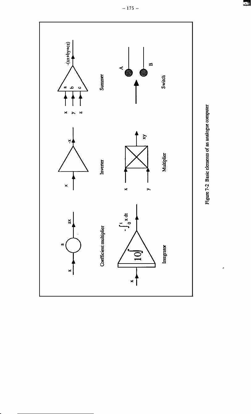
appropriate device to be used. Figure 7-2 shows some of the basic elements used in this
study to construct the nonlinear systems. Because the analogue computer can only
integrate a function with respect to time (rather than differentiate it), a differential equation
has to be solved for the highest derivative in the equation.
In this study, several nonlinear SDOF systems, having either nonlinear stiffness or
nonlinear damping which are believed to be frequently encountered in practice, are
simulated on an analogue computer in order to investigate the dynamic behaviour of a
system having these types of nonlinearity.
-- 165 --
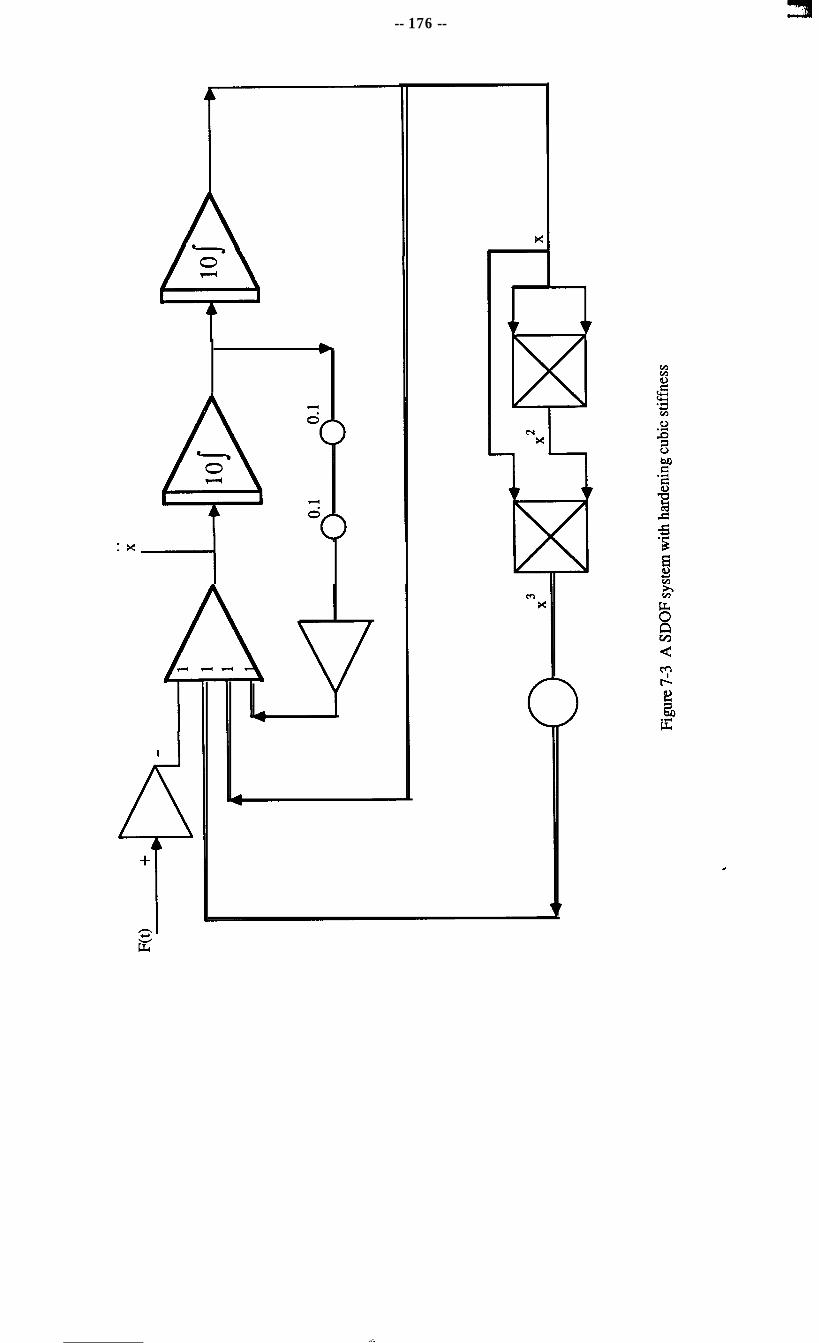
(1) A SDOF System with Hardening Cubic Stiffness
A SDOF system with hardening cubic stiffness and linear viscous damping is governed
by the following differential equation of motion:
% + 2r;c@ + coo2 (x+px3) = F(t) (7-3)
where 5 - viscous damping ratio of the system;
o0 - natural frequency of the system;
j3 - cubic stiffness coefficient;
F(t) - function of the excitation force.
In order to set up the analogue circuit for this system, equation (7-3) should be rearranged
into:
? = - ( -F(t) + 2@q,k + oo%+ coo2px3} (7-4)
In this study, the viscous damping ratio of the system is chosen as 0.005 and the natural
frequency as 10 rad/sec. The analogue circuit which simulates equation (7-4) is shown in
Figure 7-3.
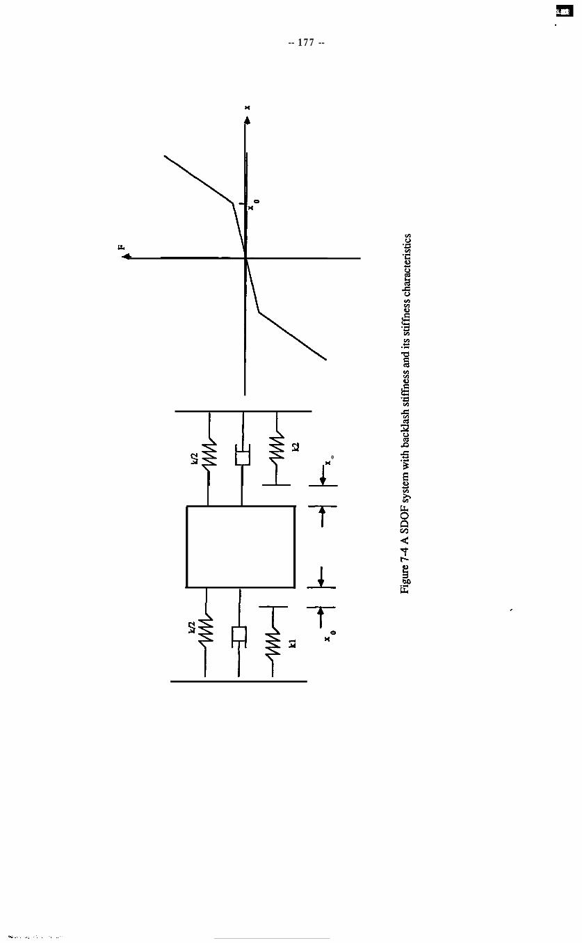
(2) A SDOF System with Backlash Stiffness
A system with backlash stiffness and linear viscous damping can be shown in Figure 7-4
and the governing equation of motion is as follows:
% + 2&i + wo2x + q(x) = F(t) (7-5)
where:
i
+ %I% x>+x()
<p(x) = 0 -xc<x<+xc
- 661()~xo xc -x0
Here, parameter xc - which defines the linear response level of the system - is called the
. .
“response limit” and a linear system will have a infinite response limit. The other
parameter 6 which symbolises the stiffness change is referred to later as “stiffness ratio”
and a zero stiffness ratio will mean a linear system.
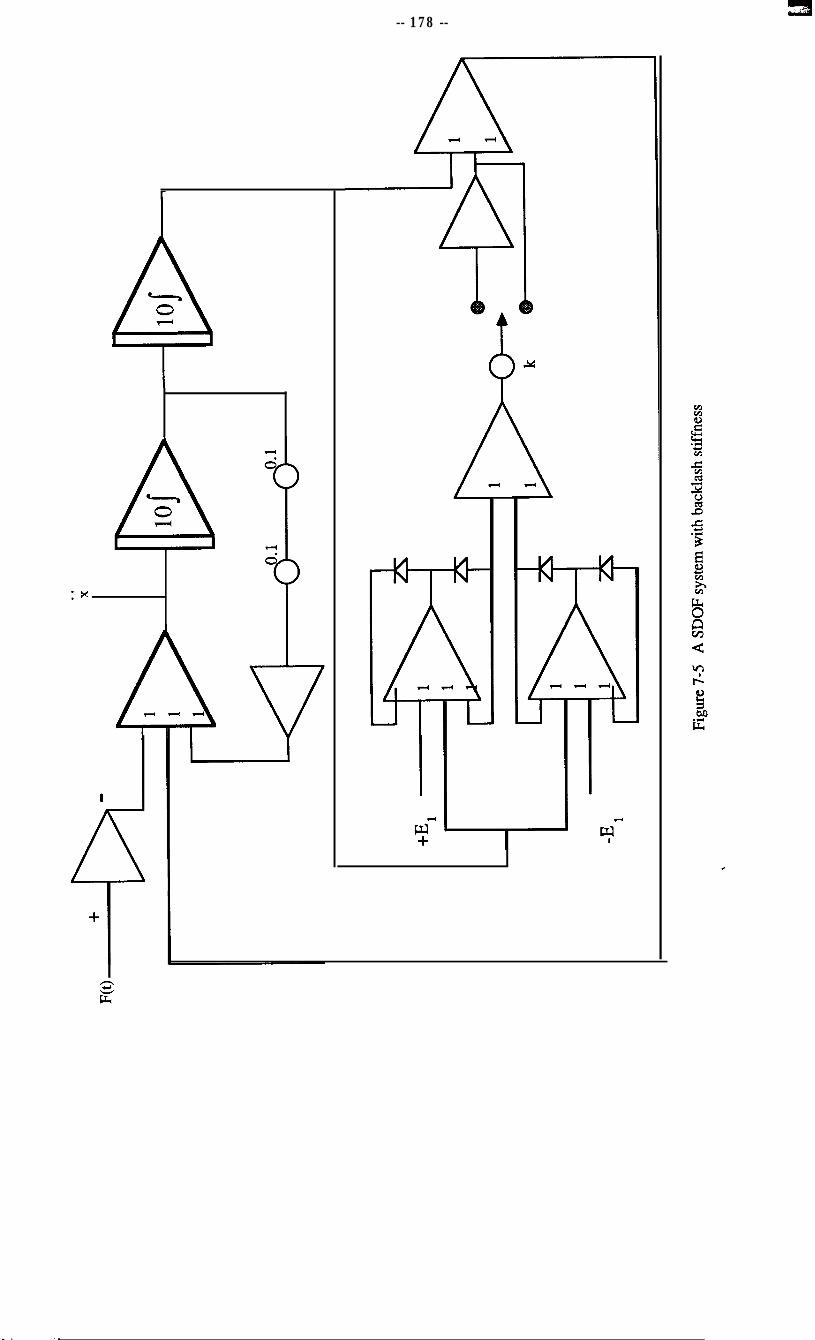
Again, in order to set up the analogue circuit for the system, equation (7-5) is rearranged
into:
;; = -{ -F(t) + 2504+ + CJ$X + q(x) ) (7-6)
With the same viscous damping ratio and the natural frequency as before, the analogue
circuit which simulate equation (7-6) is shown in Figure 7-5.
(3) A SDOF System with Piece-wise Stiffness
Piece-wise stiffness is a kind of nonlinear stiffness which is fairly often encountered in
practice. It differs from cubic stiffness in that its stiffness change is not continuous and
the stiffness effectively consists of a combination of several linear stiffnesses in different
response ranges. The backlash stiffness discussed immediately above is a type of
piece-wise stiffness. A system with piece-wise stiffness and viscous damping is governed
by the following general equation of motion:
j; + 250,~ + q(x) = F(t) (7-7)
where q(x) is a piece-wise function, contributing nonlinear stiffness effects and, for
instance, this function becomes as below for a bilinear stiffness:
Again, in order to set up the circuit for a system with piece-wise stiffness, equation (7-7)
is rearranged into:
-- 167 --
ii = -( -F(t) + 2&1.+,i + q(x) ) (74)
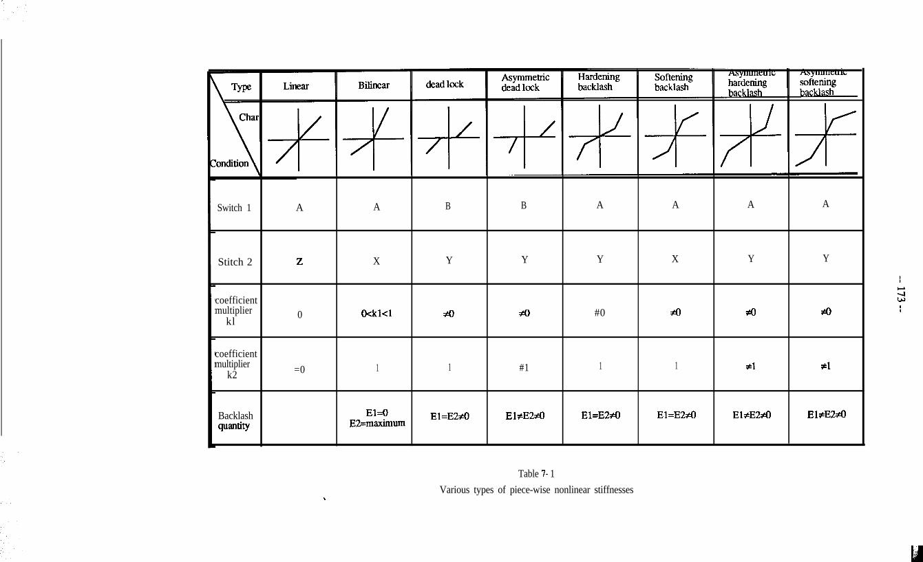
Figure 7-6 shows an analogue circuit which enables us to simulate various types of
piece-wise stiffness due to the positions of those switches indicated in this Figure. The
piece-wise stiffnesses this circuit enables us to simulate are shown in Table 7- 1.
(4) A SDOF System with Nonlinear Quadratic Damping
Nonlinear damping appears to be encountered less often than nonlinear stiffness in
practice, although this is actually not the case. This prejudice is partly due to the fact that
some dynamic structures are not significantly damped so that nonlinear damping may not
contribute as much as nonlinear stiffnesses and hence is not paid as much attention as
nonlinear stiffness. For fairly heavily damped structures, nonlinear damping is surely
another domain of nonlinearity which cannot be overlooked.
Quadratic damping is one of the many types of nonlinear damping encountered in practical
vibration problems. A SDOF system with linear stiffness and quadratic damping can be
described by the following equation of motion:
j;+aIxIx+o,Sr=F(t) (7-9)
where a is the quadratic damping coefficient.
Equation (7-9) can be rearranged to be suitable for the analogue set-up:
j;=_ (- F(t) + a I i I f + a+,%~) (7-10)
and the corresponding analogue circuit for this SDOF system having quadratic damping is c
shown in Figure 7-7.
-- 168 --
7-5 THE FREQUENCY RESPONSES OF THE NONLINEAR SYSTEMS
Once a nonlinear system is simulated on an analogue computer, a FRF measurement can
be performed as if it were a practical structure. As suggested earlier in this Chapter,
sinusoidal excitation is selected to provide the input (force) to the system and the
consequent acceleration (or velocity, displacement) of the system is regarded as that of the
structure due to the sinusoidal input force. The frequency response function (FRF) of the
nonlinear system can then be obtained from a frequency response analyser. The post
measurement modal analysis will then be based upon the FRF thus obtained.
However, the most important difference between measuring a simulated nonlinear system
and measuring a practical structure should be noted here. When sinusoidal excitation is
applied to measure a simulated nonlinear system without using a shaker, the force level
for the entire measurement will be constant (mainly controlled by the generator) as the
nonlinear property of a shaker which distorts the force level is not present. Therefore, the
nonlinearity could be readily exposed and its identification is relatively easy. However,
for the measurement of a practical structure, the force level will tend to vary near any
resonances which, in turn, influences the effect of the nonlinearity on the frequency
response function data.
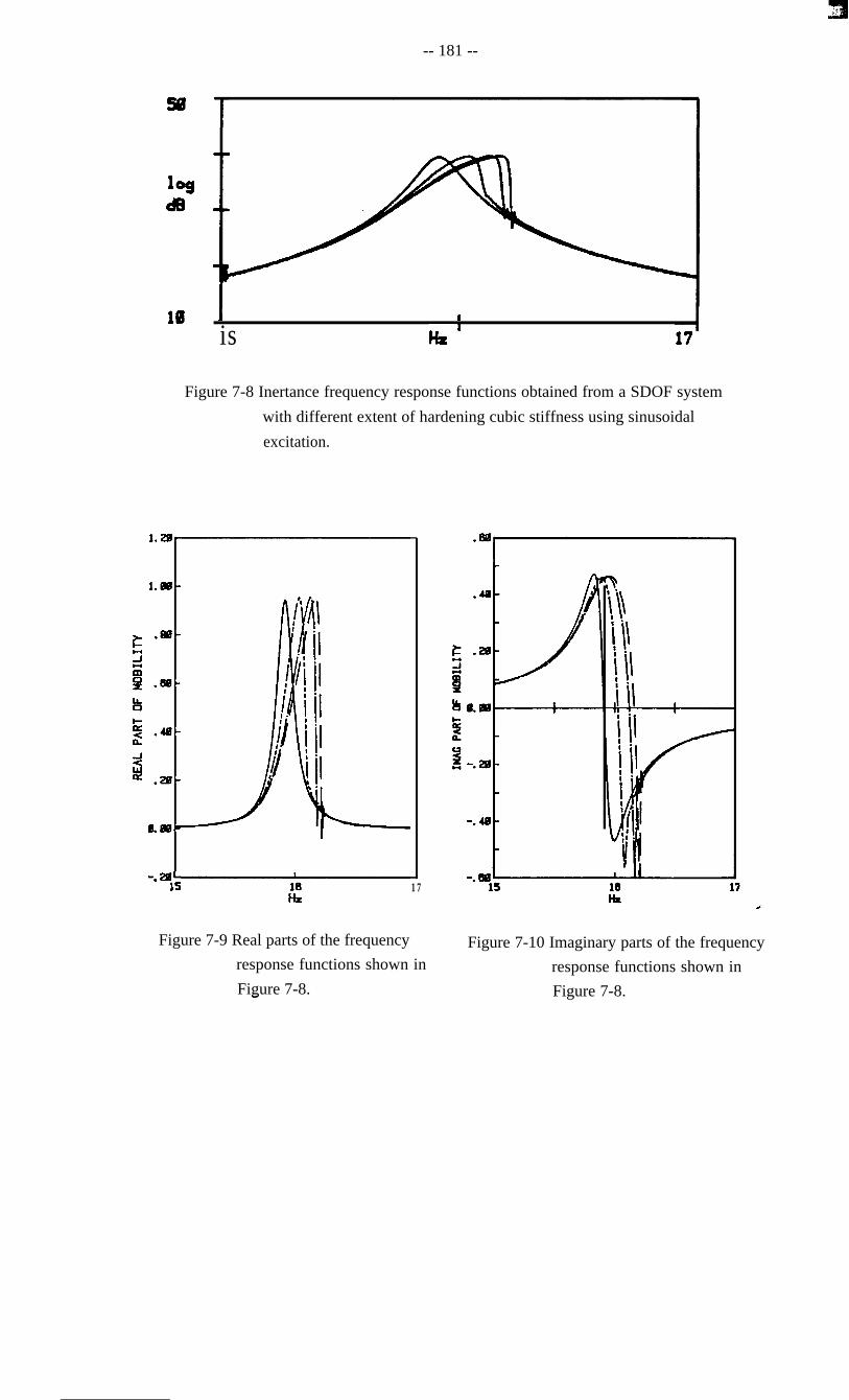
Figure 7-8 shows the inertance-type frequency response functions obtained from a SDOF
analogue system measured using sinusoidal excitation and Figures 7-9 and 7-10 present
the corresponding real and imaginary parts plots. The system contains hardening cubic
stiffness with different cubic stiffness coefficients. Figure 7-11 shows the frequency
response functions of the same system with an unchanged cubic stiffness coefficient c
while the excitation force level varies and again, the corresponding real and imaginary
parts are shown in Figures 7-12 and 7-13. It can easily be seen from Figures 7-10 to 7-13
that increasing the cubic stiffness coefficient has an identical effect on the frequency
response function data of the system to increasing the excitation force level. Hence,
-- 169 --
although the extent of nonlinearity in practice is virtually impossible to change arbitrarily
as the simulated system can be, the effect of different extent of nonlinearity on the the
frequency response function of the nonlinear system can still be demonstrated by varying
the excitation force level so that the nonlinearity can be fully exposed and identified.
For a SDOF system with backlash stiffness, the frequency response function due to
sinusoidal excitation is influenced by the nonlinearity and the excitation force level in a
slightly different way to that seen for the cubic stiffness case. There exist three possible
conditions for this simulated SDOF system to vary and they are (a) the excitation force
level, (b) the response limit and (c) the stiffness ratio - both parameters having been
defined in equation (7-5). The frequency response of this system due to the change of
each condition is studied.
Figures 7- 14 to 7- 16 show the frequency response functions and their corresponding real
and imaginary parts obtained from a SDOF analogue system by using sinusoidal
excitation. The system containing hardening backlash stiffness has an unchanged stiffness
ratio and response limit as the excitation force level varies. The comparison of Figure
7-14 with Figure 7-11 will reveal the different effects of excitation force level on the
frequency response functions in these two cases, although they are all hardening-type
stiffness. For the cubic stiffness case, the frequency response function is affected
continuously by the excitation force level and this effect becomes greater as the excitation
frequency approaches the resonance frequency. However, the effect of increasing the
excitation force level for the backlash stiffness case does not show up unless the response
of the system exceeds a certain value, and this value is relevant to the excitation force
level itself. The difference discovered here could be a useful indication of distinguishing
between these two types of hardening stiffness. c
Figure 7-17 shows the frequency response functions of the same system containing
backlash stiffness with an unchanged stiffness ratio and a constant excitation level while
the response limit varies. It is evident by comparing Figure 7-17 with Figure 7-14 that
-- 170 --
the response limit varies. It is evident by comparing Figure 7-17 with Figure 7-14 that
decreasing the response limit of the system will have a similar effect on the frequency
response function to increasing the excitation force level. Figure 7-18 shows the
frequency response functions with an unchanged response limit and a constant excitation
level while the stiffness ratio of the system varies. It is interesting to note that the
consequence of different stiffness ratios does not show up until the response reaches a
certain level - which is believed to be the response limit of the system - and the frequency
response functions diverge more from the one without nonlinearity as the stiffness ratio
becomes bigger. For nonlinear damping cases, such a SDOF system also simulated on
analogue computer with quadratic damping, measurement can be carried out similarly
using sinusoidal excitation. Figure 7-19 shows the FRF data with different extent of
quadratic damping. It is evident that the natural frequency of the system changes little,
while the response is obviously governed by the damping extent.
As suggested above, the frequency response of a nonlinear system due to random
excitation will appear to be that of a linear system. This is because most types of
nonlinearity are excitation amplitude-dependent while the random force signal has
randomly varying force amplitude and phase angle. Therefore, the response of a nonlinear
system due to random excitation becomes an averaged result due to the different force
amplitude and as a consequence, the effect of the nonlinearity is linearised. To appreciate
this, random excitation is used in the measurement of the simulated nonlinear systems
discussed above. The measured frequency response function data eventually show
apparently linear behaviour for the nonlinear systems.
To understand fully the linearisation consequence of random excitation tests, questions
about the Fourier Transform algorithm have to be answered. As the Fourier Transform is c
a linear operation, suggestions of this algorithm linearising the nonlinearity could be
found in some literature[ 611. In this study, a special investigation was carried out:
sinusoidal excitation is used for the nonlinear systems while the frequency response
analysis is performed by an FFT analyser. It is found that as the excitation frequency
-- 171 --
sweeps, the frequency response function obtained by FFI’ exhibits exactly the same
results as shown in Figures 7-8 to 7-17 which are obtained from frequency response
analyser. This verifies the discussion in the earlier part of this Chapter - the Fourier
Transform is not responsible for the linearisation of the effect of nonlinearity in
measurement using random excitation. It is the randomness of the force amplitude and
phase angle of the input signal which linearise the response of a nonlinear system and
makes the system behave as a linear system
7-6 CONCLUSIONS
Nonlinearity is a widely-encountered phenomenon in practical dynamic structures. It is
sometimes neglected because of its small extent and little contribution to the vibration
response, but for many other cases, lack of proper means to deal with the nonlinearity
could be the primary reason for ignoring it.
Theoretically, the main difficulty introduced by the nonlinearity is that the superposition
principle whereby the response of a system to different excitations can be added linearly is
violated for nonlinear systems. As a consequence, the dynamic characteristics of
nonlinear structures become excitation-dependent and much less easily predicted.
It is believed that theory has been highly developed for those nonlinear systems whose
equations of motion are expressible analytically. There are currently quite a number of
methods which are available to examine the vibration behaviour of a known nonlinear
system.
However, since the nonlinearity inherent in vibrating structures is difficult to identify and c
even much more difficult to quantify, such theory is often not directly applicable to
experimental modal analysis because of the absence of explicit equations of motion. The
efforts of nonlinearity study in practical vibration analysis are then focussed on the
detection and the identification of nonlinearity in structures from measured FRF data
-- 172 --
Since the effects of most kinds of nonlinearity frequently encountered in structural
dynamics are characteristically variable due to the external excitation, the first problem of
the nonlinearity investigation will be to choose a proper excitation force so that the
nonlinearity could easily be exposed and then detected and identified. Amongst those
excitation methods currently widely used in vibration study, the sinusoidal excitation
method is strongly favored for nonlinearity investigation.
Analogue computer simulation is advantageous for nonlinearity investigations. This is
mainly because a nonlinear system can easily be simulated on an analogue computer and
the parameters of the system can then be conveniently adjusted to represent different
extent of nonlinearity. Hence, the response of the simulated nonlinear system can be
obtained and the vibration characteristics of the nonlinear system can then be thoroughly
investigated which, in turn, will be referenced for the nonlinearity investigation of the
practical structures.
SDOF systems with some frequently encountered types of nonlinearity are successfully
simulated on an analogue computer. Among those types of nonlinearity are cubic
stiffness, backlash stiffness, quadratic damping and various kinds of piece-wise stiffness.
Measurement using the sinusoidal excitation method can then be performed to obtain the
frequency response functions of these nonlinear systems. The refined modal analysis can
be carried out to detect and identify the nonlinearity by analysing these measured
frequency response function data and this will be extensively studied in the next Chapter.
Figure 7-l Linearisation effect of random excitation test
-- 175 --
x
-- 176 --
:X
40
--I
c
_,-.
-- 177 --
as
I I
sfe3a
0w
-I!--f
__!I!--7
0n
c
-- 178 --
40
:x
I
+
c
:X
+
hcL
-- 180 --
t
I
A
+c
-- 181 --
10 I I
is Hd
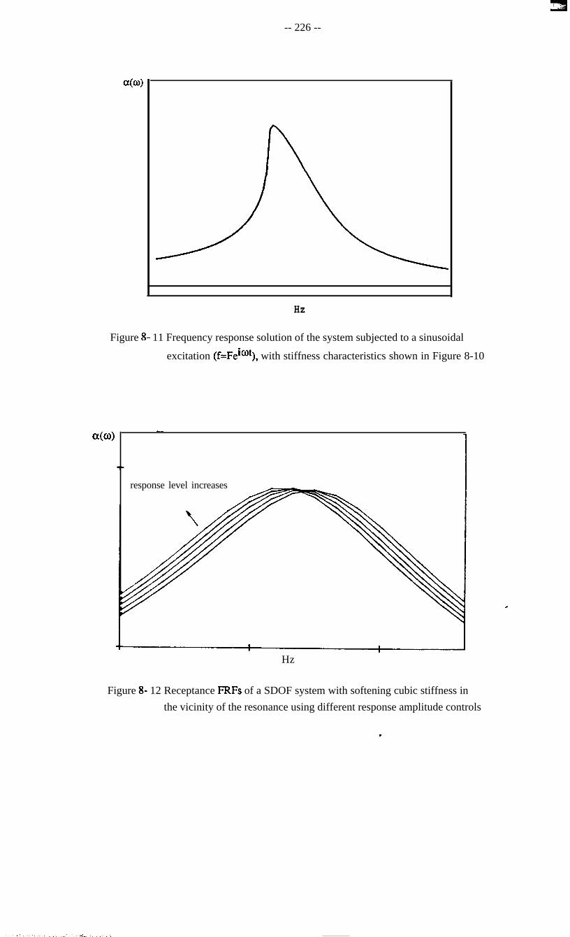
Figure 7-8 Inertance frequency response functions obtained from a SDOF system
with different extent of hardening cubic stiffness using sinusoidal
excitation.
I-
I-
I-
I-
I-
t-
I-
Lis 17
Figure 7-9 Real parts of the frequency
response functions shown in
Figure 7-8.
Figure 7-10 Imaginary parts of the frequency
response functions shown in
Figure 7-8.
-- 182 --
10 1 I
is Hr‘ 17
Figure 7- 11 Inertance frequency response functions obtained from a SDOF system
with hardening cubic stiffness using different sinusoidal excitation
levels.
-.a‘115 IE
Figure 7-12 Real parts of the frequency
response functions shown in
Figure 7- 11.
-. 40 -
-. 6815 16 17
I4c
Figure 7-13 Imaginary parts of the frequency
response functions shown in
Figure 7- 11.
-- 183 --
J I
is H8’ 17
Figure 7-14 Inertance frequency response functions obtained from a SDOF system
with hardening backlash stiffness using different sinusoidal excitation
levels.
is
Figure 7-15
16 17
Real parts of the frequency
response functions shown in
Figure 7- 14.
.4&l-
~0.W~ I1
5su -.2m-
-. 4% -
Figure 7- 16 Imaginary parts of the frequency
response functions shown in
Figure 7- 14.
_
-- 184 --
logde
10 I I
is
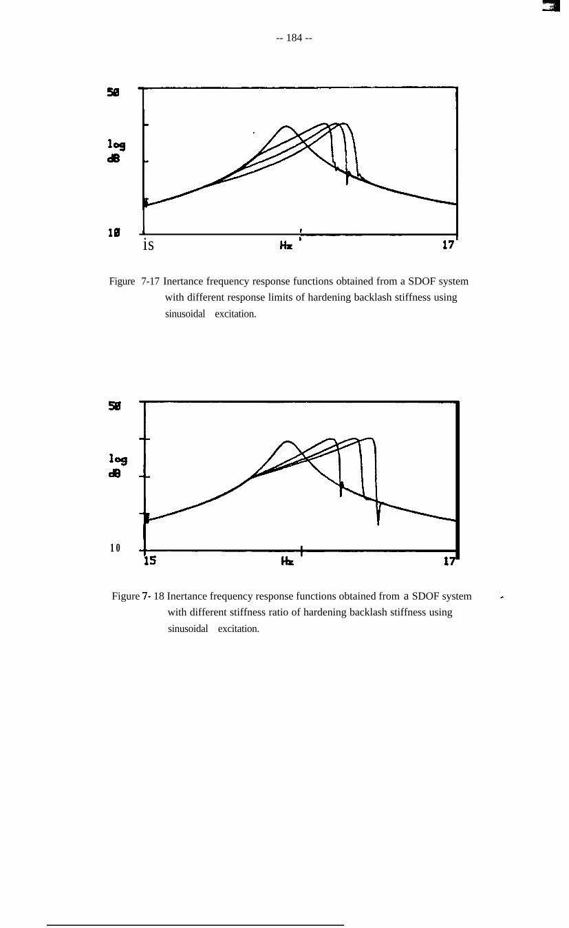
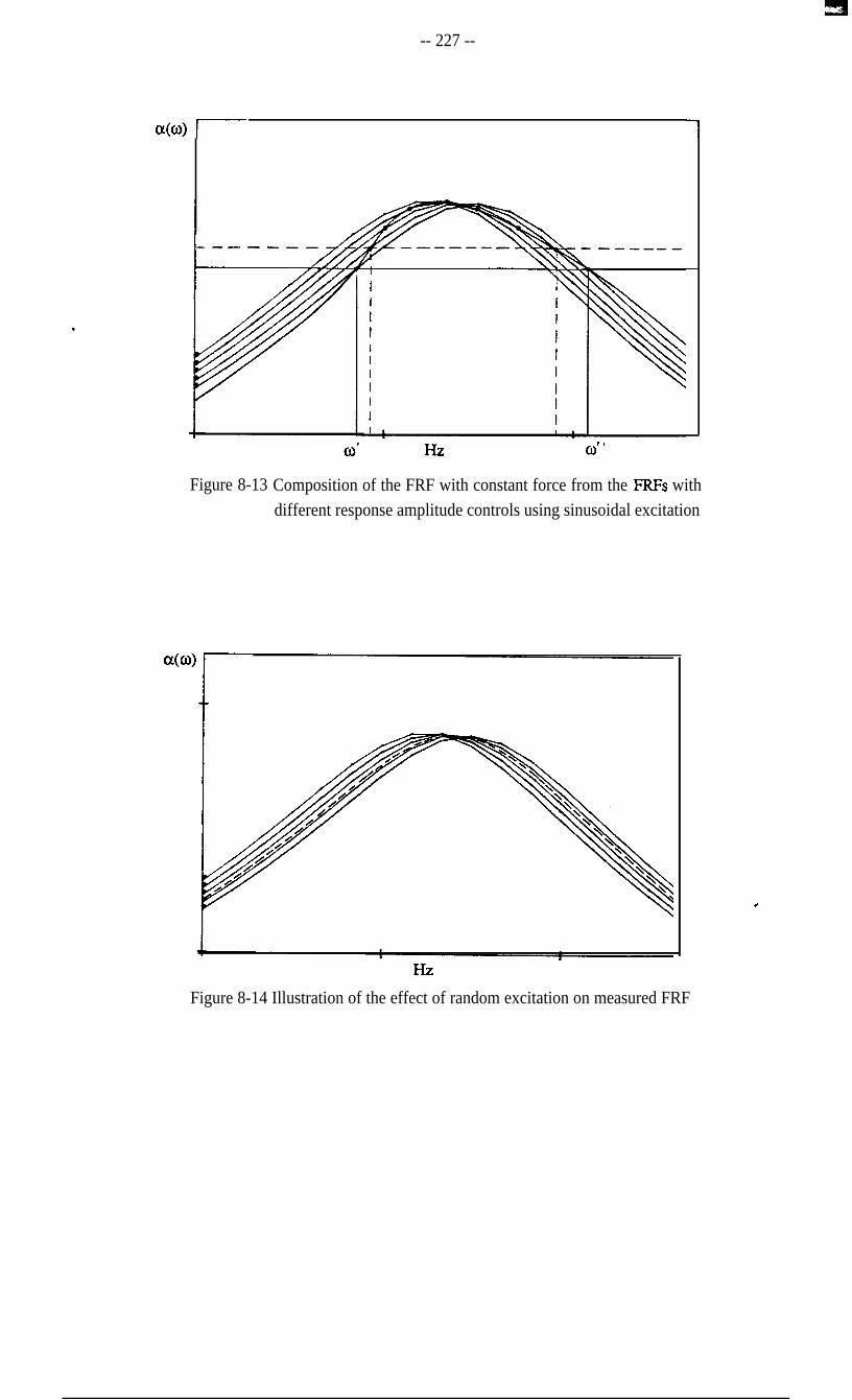
Figure 7-17 Inertance frequency response functions obtained from a SDOF system
with different response limits of hardening backlash stiffness using
sinusoidal excitation.
10
Figure 7- 18 Inertance frequency response functions obtained from a SDOF system
with different stiffness ratio of hardening backlash stiffness using
sinusoidal excitation.
50
109
d6
1015 17
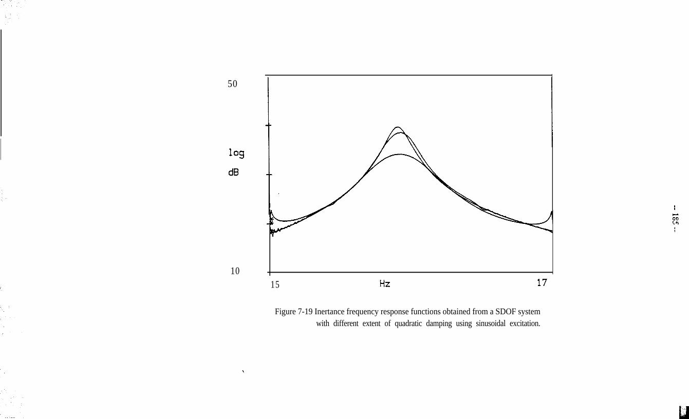
Figure 7-19 Inertance frequency response functions obtained from a SDOF systemwith different extent of quadratic damping using sinusoidal excitation.
c
-- 187 --
CHAPTER 8
MODAL ANALYSIS OF NONLINEAR SYSTEMS
8-l CURRENT METHODS AND APPLICATIONS OF MODAL ANALYSIS FOR
NONLINEAR SYSTEMS
Once it is suspected that a structure or a system is nonlinear, and measurement is carried
out as discussed extensively in the last Chapter, it is necessary to analyse the frequency
response function data taking account of the effect of possible nonlinearity. The
application of modal analysis methods to such FRF data depends upon the different
requirements on the nonlinearity investigation of the system. Generally speaking, there
are three possible requirements in practice for the results of modal analysis of a nonlinear
system. First, a linearised model may be required whose vibration response will be as
close as possible to the actual vibration response of the nonlinear system. Second, the
type of nonlinearity might need to be identified in order to enable the possible
establishment of a correct mathematical model of the nonlinearity and to seek the
possibility of predicting the vibration response of the nonlinear system to a wide range of
excitation conditions. Third, the identified type of nonlinearity is to be quantified in some
extent.
It is believed that the first requirement - to obtain a linearized model for a nonlinear system
without seeking the nature of the nonlinearity - is comparatively easy to achieve. In fact, a
family of frequency response functions with different random excitation force levels could *
always be measured, as suggested in the Chapter 7, and a conventional linear modal
analysis algorithm be employed to build up a series of models, each of them representing
the vibration behaviour of the nonlinear system under conditions of a certain excitation
force level. It is worth noting that such an investigation does not tell the nature and extent
-- 188 --
of the nonlinearity but, instead, it simplifies the nonlinearity problem by a piecewise
linearization approach.
However, practice is often confronted with the requirement of understanding the nature,
and even the extent, of the nonlinearity of a dynamic structure. Hence, current modal
analysis efforts are directed towards the detection of nonlinearity, and the identification of
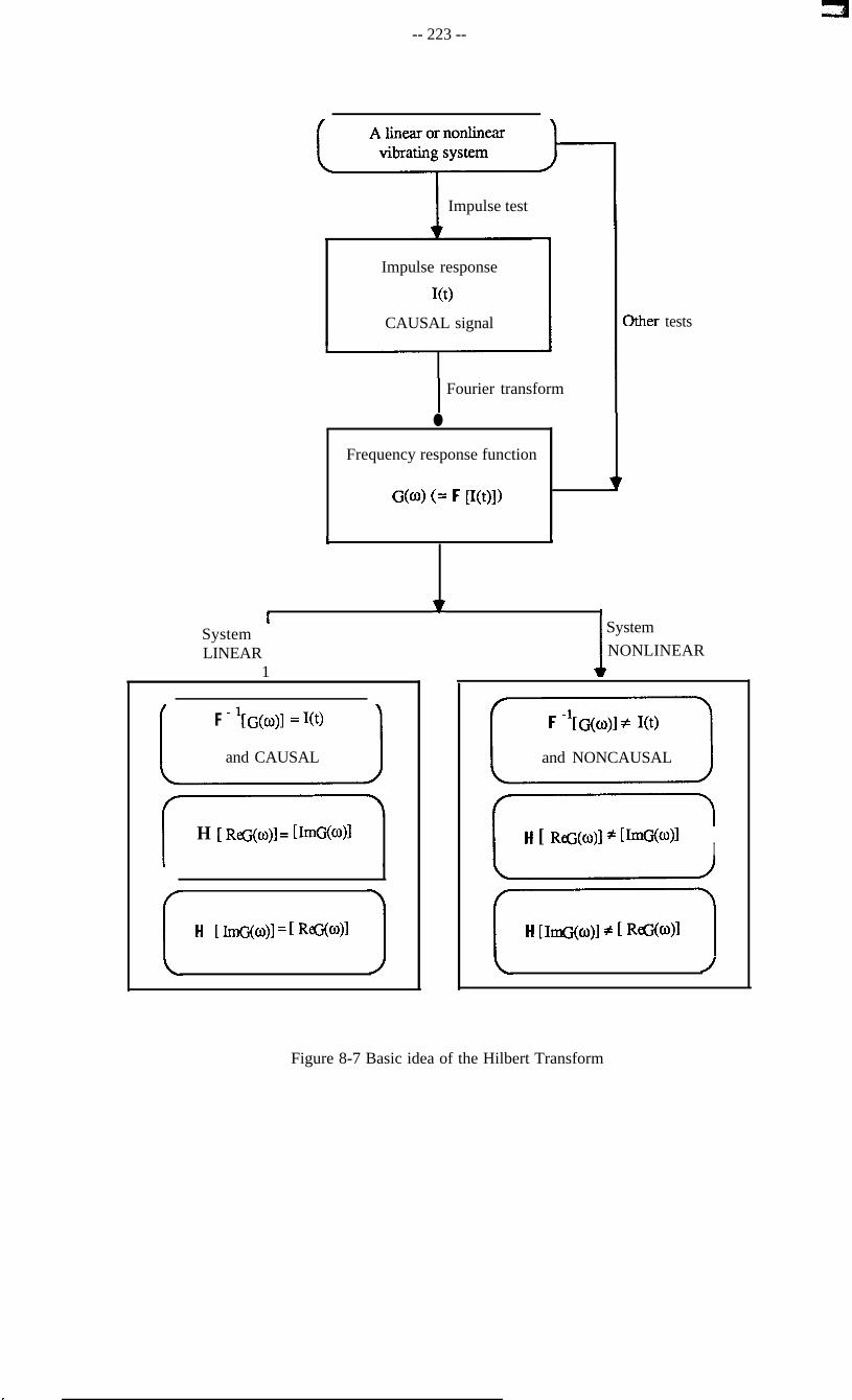
the type and extent of nonlinearity in structures. To summarize, the following three
questions are to be answered by the appropriate application of modal analysis methods to
structures which might be nonlinear (Figure 8-l).
(1) Is the system or structure nonlinear?; (detection)
(2) If yes, what kind of nonlinearity does it exhibit?; and (identification)
(3) What is the extent of the nonlinearity? (quantification)
A large number of papers dealing with nonlinearity can be found in the literature in recent
years. As far as the detection and the identification of nonlinearity from the modal test data
is concerned, the methods commonly employed nowadays can be summarised below. It
is important to bear in mind that sinusoidal excitation is preferred in modal tests for all
these methods in order to let the nonlinearity be properly exposed rather than be averaged
out as happens in random excitation conditions. The advantages and disadvantages of
those methods currently used and summarised below will be discussed and the direction
of further developments will then be pointed out.
8-l-l Bode Plots
The basis of using Bode plots to detect the possible existence of nonlinearity, and to
identify it, is that the nonlinearity should systematically distort the frequency response c
function data and its real and imaginary parts from the form of the corresponding linear
system’s FRF data. As the linear system’s frequency response function is very well
recognized, the possible existence of nonlinearity could then be revealed by examining the
abnormal behaviour of the real and imaginary parts of the frequency response function
-- 189 --
data.
A typical example of nonlinearity being evident in the Bode plot is provided by the
frequency response function data shown in Figure 7- 11 and its corresponding real and
imaginary parts shown on Figures 7-12 and 7-13. The system from which these data are
derived has hardening cubic stiffness and it can be seen that this nonlinearity is clearly
exposed on the data. Similarly to this cubic stiffness case, the frequency response
function and its corresponding real and imaginary parts obtained from another SDOF
system, this time with backlash stiffness, are shown in Figures 7-14 to 7-16. Again, the
existence of the nonlinearity is apparent from the systematic distortion in the plots.
Although Bode plots of the frequency response function data can reveal the existence of
possible nonlinearity in most cases, it is after all merely a straightforward presentation and
no analysis of nonlinearity is involved, As a consequence of its simplicity, this method
usually cannot distinguish one type of nonlinearity from the other - e.g. the cubic stiffness
and backlash stiffness - when their effects on the frequency response function data are
fairly similar. Therefore, Bode plots can only be used to provide a rough and basic
examination of the existence of nonlinearity.
8-l-2 Reciprocal of Frequency Response Function
The Reciprocal of frequency response function data, which was previously discussed
briefly in Chapter 4, is offered as an alternative to modal analysis by the Nyquist circle fit.
It is based upon an assumption of SDOF behaviour. Basically, it is supposed that,
neglecting the residual effects of all other modes, the p mode of the frequency response
function (receptance) data of a structure will yield: c
oljl =Pjl
6$ co* + iTpr2
where: aj, is the receptance between test points j and 1;
(8-l)
-- 190 --
pjl is modal constant;
cer2 is the natural frequency;
TJ, is the damping loss factor.
Although the modal constant is in theory a complex quantity, it is often effectively real
and is treated thus here for this approach. The corresponding reciprocal of receptance &ta
is:
(l/ajJ =q- a2 + iqpr2
Pjl(8-2)
= Re(l/ajJ + h(l/ajJi
Perhaps the most significant advantage of using the reciprocal of receptance data is that
the mass and stiffness characteristics (natural frequency and modal constant in modal
data) and damping property (damping loss factor in modal data) are separated out into the
real and imaginary parts of the data respectively and hence, they can be dealt with
separately. In this case, the estimation of natural frequency and modal constant will be
considerably less affected by the damping loss factor than happens in the Nyquist
circle-fit or MDOF curve-fit, since this estimation is carried out only on the real part of the
reciprocal of receptance data, and which is physically quite reasonable. Similarly for the
estimation of damping loss factor, for the same reason. In addition, the extraction of
modal data from the reciprocal of the receptance data will not require the condition of
equal frequency spacing of the data which Nyquist circle-fit does.
The significant advantage of using the reciprocal of the receptance data becomes evident c
when modal analysis is made of FRF data from systems with nonlinearity. In these cases,
the effects of a nonlinear stiffness will show up on the real part of the reciprocal of
receptance data while the imaginary part of the data will be dominated by the effect of the
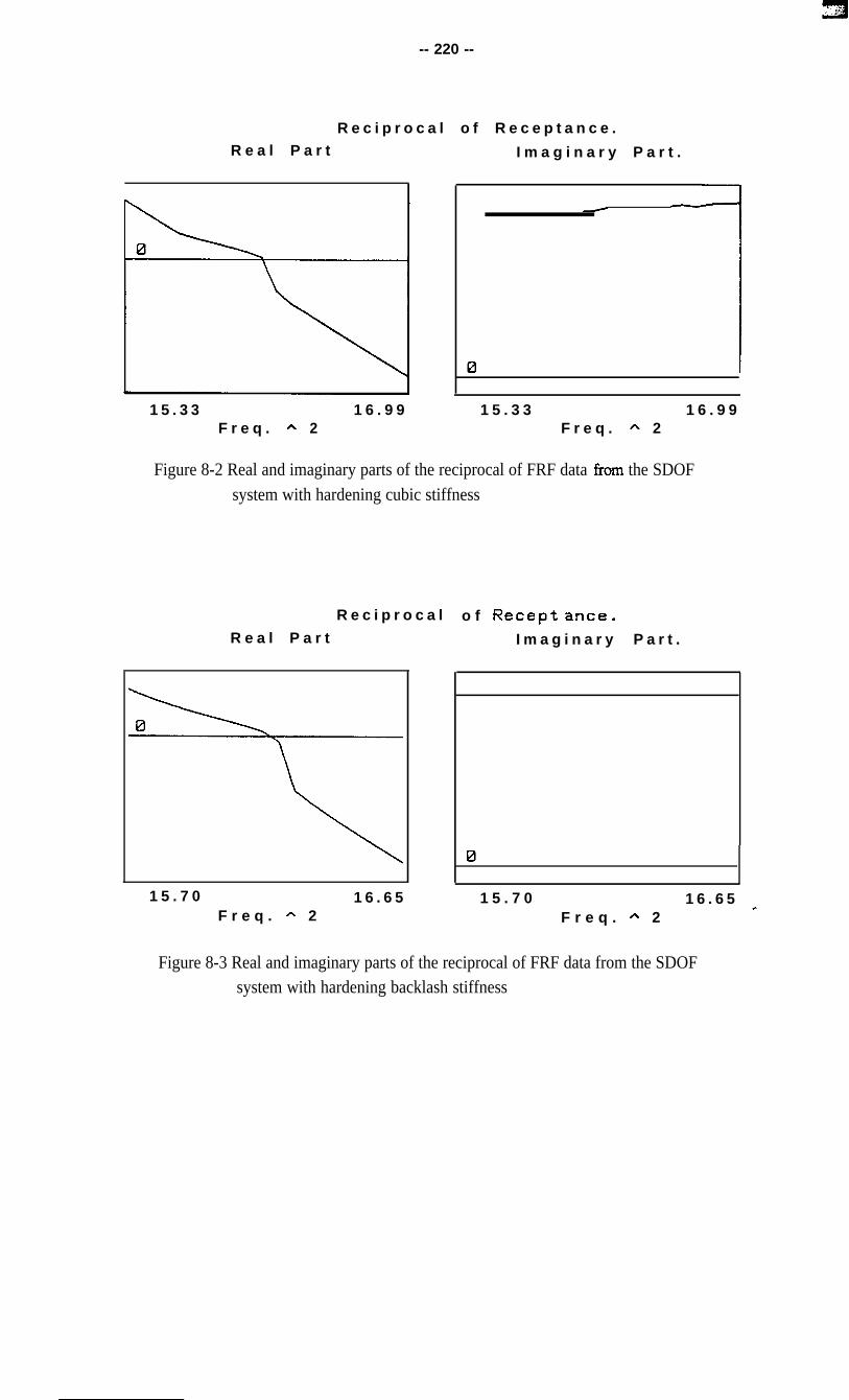
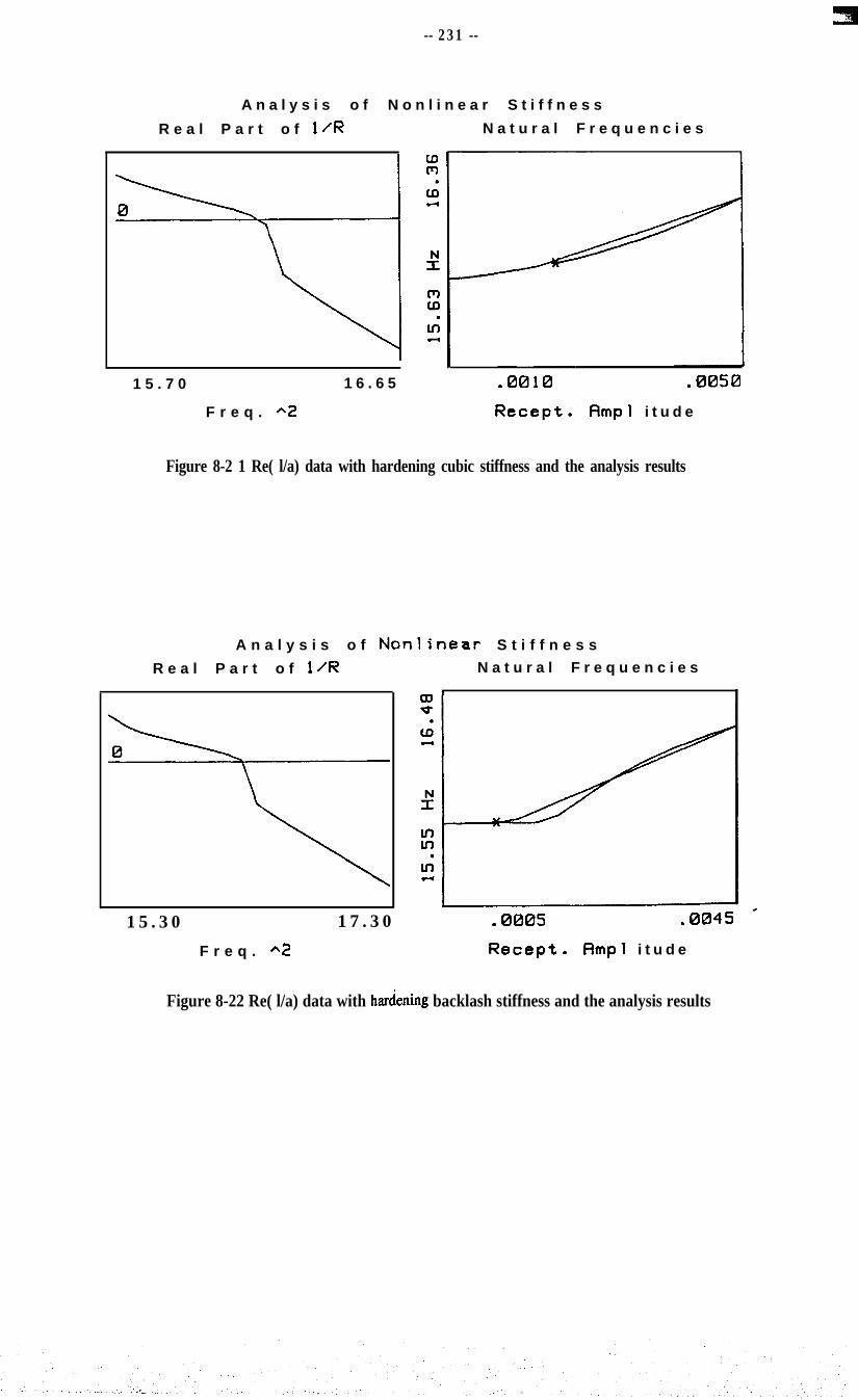
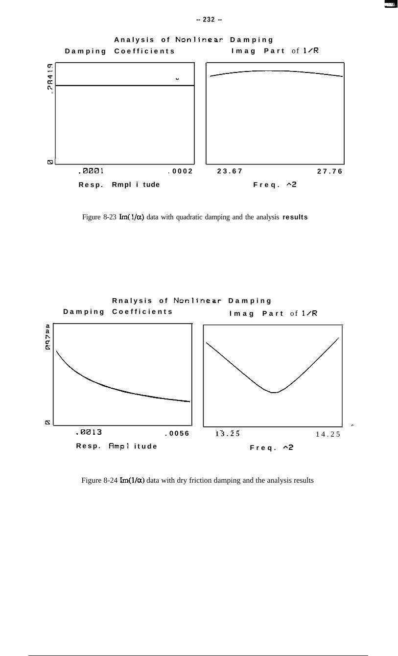
damping. Figure 8-2 shows the real and imaginary parts of the reciprocal of FRF data of
-- 191 --
a SDOF system with hardening cubic stiffness. It can be seen that the effect of the
nonlinear stiffness distorts the real part data noticeably but the imaginary part remains just
as for the linear case since the system here does not have any nonlinearity in the damping.
In Figure 8-3, similar real and imaginary parts of the reciprocal of FRF data for a SDOF
system with hardening backlash stiffness are presented. Again, the effect of the nonlinear
stiffness is clearly observed confined to the real part data.
This characteristic - that the effect of stiffness nonlinearity only shows up in the real part -
is in contrast with the standard FRF data format where the effect of any type of
nonlinearity will influence both its real and imaginary parts equally (e.g. the real and
imaginary parts of inertance FRF data). This is due to the fact that the real and imaginary
parts of the FRF data are related to each other and it will be seen in later discussion that
the Hilbert transformation makes use of this relationship between the real and imaginary
parts of the FRF data to investigate nonlinearity.
S-l-3 Modal Analysis and the Isometric Damping Plot
The isometric damping plot is one of the simpler methods available for the modal analysis
of nonlinear systems. Its application to the detection and identification of nonlinearity
relies on the argument that the nonlinearity will distort the spacing of the frequency
response function data along the Nyquist circle from their positions when no nonlinearity
exists. Its effect is unlike noise on the measurements, which also tends to distort the FRF
data, because the distortion provoked by nonlinearity is systematic rather than random.
Due to this character of systematic distortion, the damping estimates will vary according
to the specific point selection around the Nyquist circle and the nature of the distortion
displayed by the different damping estimates indicates the existence of nonlinearity. The -
following analysis seeks to explain the mechanism in detail.
It is well known that the damping loss factor for a vibration mode can be estimated by
curve-fitting the Nyquist circle (as shown in Figure 8-4) and using the following
-- 192 --
equation:
where o8 and ob are frequencies for two data points, one before and one after the
identified natural frequency. Also, it is known that for the FRF data from a linear system
without noise pollution, the damping estimate in equation (8-3) will theoretically be the
same no matter what pair of points on the Nyquist circle are chosen.
If the system is nonlinear, however, and the nonlinearity distorts the spacing of the FRF
data on the Nyquist circle systematically, as noted above, the then the damping estimates
from equation (8-3) will also vary systematically depending on the different points
selected, and variation in damping estimates becomes a good indication of the
nonlinearity. Figure 8-5 shows the Nyquist plot of the FRF data for a SDOF system with
hardening cubic stiffness and the corresponding isometric damping plot. It can be seen
that the nonlinear stiffness produces typical damping variation on the isometric damping
plot. In Figure 8-6, a similar Nyquist plot of the FRF data from a SDOF system with
hardening backlash stiffness and the isometric damping plot are shown. Again, the
damping variation in the isometric damping plot caused by the nonlinearity exhibits a
strong characteristic.
8-l-4 The Hilbert Transform
The Hilbert transform is a method for calculating the imaginary part of a complex
frequency response function from its real part (and vice versa), under certain conditions.
According to the Cauchey-Rieman theorem, a mathematically hatmonic complex analytical ’
function possesses the property that its real part can be derived from its imaginary part
and vice versa. This relationship is known as a Hilbert transform pair. In recent years, the
Hilbert transform technique has been borrowed from control engineering and applied to
vibration research for the identification and analysis of nonlinearity in structural
.I . ., , .‘..
-- 193 --
dynamics. In the following, the definition of the Hilbert transform will be briefly
reviewed and the basis for its application to modal analysis will be outlined, together with
several application examples.
S-141 The Principle of the Hilbert Transform
The Hilbert transform of a mathematical function f(x) is defined as an integral and is
denoted as H :00
F(x) = l/rt f(x’) dx’/(x’-x)J-00= HVOOI (8-4)
The integral F(x) is a linear functional of f(x) and it can be shown from the theory of
random vibration that the integral in equation (8-4) can be obtained by convolving the
mathematical function f(x) with (-7tx)-‘, namely,
F(x) = (-~/RX) f(x) (8-5)
or H [f(x)] = (-~/XX) f(x)
Since the Fourier transform of (- l/rrx) is i(S g n co), where s g n is a sign function and i is
imaginary unity, it can be said that the Hilbert transform is equivalent to a particular kind
of filtering in which the amplitude of the spectral components are left unchanged but their
phases are altered by 7r/2. Thus, the application of the Hilbert transformations twice in
succession will reverse the phase of all components and the results will be the negative of
the originals:z
f(x) = -(-l/xx) F(x) (8-6)
00
f(x) = -~/IF J_F(x’) dx’/(x’-x) (8-7)
-- 194 --
orf(x) = - H [WI
8-l-4-2 Basis of the Application of the Hilbert Transform to Modal Analysis
The frequency response function of a dynamic system G(o), which is a function of
frequency o, is the Fourier transform of I(t), the impulse response function of the system
which is a time varying functionWI:
G(o) = J I(t) dot dt-00 (8-8)
or G(o) = F [I(N
where F denotes the Fourier transformation in this work.
Since the impulse response I(t) from a linear system is real and causal (a system is causal
if, for any input, the response at any instant of time does not depend upon the future
input: a linear dynamic system should always be causal), it can always be split into even
and odd parts:
I(0 = w,,, + 1(0,&-j
= (I(t) + I(-t))/2 + (I(t) - I(-t))/2
and the even and odd parts can be linked together by the following equation:
(8-9)
wodd = W,, s 9 n (0
Since the Fourier transform of the sign function s g n (t) is:
F [sgn(t)] =-i/no (8-l 1)
the Fourier transformation of both sides in equation (8- 10) yields:
F [I(Ooddl = F [I(~),,1 F [s g NOI
= F [I(t),,1 (-i/n@
(8-10)
(8-12)
-- 195 --
It can be validated theoretically[74]1[75],[76] that, for a linear dynamic system, the real
part of the frequency response function G(o) is the Fourier transform of the even part of
the impulse response function I(t), and the imaginary part of G(o) is the Fourier
transform of the odd part of I(t), namely:
Re(GW) = F D(t>,,l
Im(G(W = F II(Oodd]
(8-13a)
(8-13b)
Thus, it can be shown as below that the imaginary part of the frequency response function
G(o) can be obtained from the Hilbert transform of its real counterpart (the same
argument holds for the other way around):
H [ReG(o)] = (4/x0) Re(G(o))
= F [ F-‘[(-i/m) ReG(o)]]
= F [b&t) W,,ll
= ImG(o)
Therefore, it is demonstrated by the above analysis that for a linear vibrating system, the
entire frequency response function can be constructed by knowledge of either its real or
its imaginary parts only or, in other words, either one of them determines completely the
vibration characteristics of the system. It should be borne in mind that although it is
suggested above that the impulse response is obtained from test, this is merely for the *
sake of simplicity to depict the theory. In practice, any kind of measurement technique
could be used and the inverse of Fourier transformation of the frequency response
function should always provide the impulse response of the system, provided this is
-- 196 --
linear and no noise pollution is involved.
If a system is nonlinear, then its impulse response from an impulse test is normally still
causal, provided the system is time-invariant as most structures in practice are. However,
the inverse Fourier transform of the frequency response function obtained from a
sinusoidal excitation, which is suggested in Chapter 7 as a favorable measurement
technique, would become noncausal due to the nonlinearity[74]~[75]. Thus, the result of
the Hilbert transform of the real part of the FRF data will not be the same as the imaginary
part of the FRF as it will be distorted by the nonlinearity, nor will the transform of the
imaginary part be the same as the real part, as illustrated in Figure 8-7.
To apply the Hilbert transform to the detection and identification of nonlinearity in
vibration studies, the frequency response function of a vibrating system from sinusoidal
test is used and the Hilbert transform of its real part can be calculated (as can its imaginary
part) and compared with its imaginary part. Any discrepancy between the Hilbert
transform of the real part of the FRF and its imaginary part will then indicate the existence
of nonlinearity, provided the computation of the Hilbert transform is accurate enough.
Once different types of nonlinearity can be simulated, studied and categorized by the
Hilbert transformation, the nonlinearity found in test data could by identified with a
reference to those categorized nonlinearity.
Figure 8-8 shows the real and imaginary parts of the FRF for a SDOF system with
hardening cubic stiffness and also the Hilbert transform of each. It can be seen that the
existence of the nonlinear stiffness results in a discrepancy between the original FRF and
the Hilbert transform counterparts. In Figure 8-9, a similar FRF of a SDOF system with
hardening backlash stiffness and the Hilbert transforms are shown. Again, the.
discrepancy caused by the nonlinearity is evident. These discrepancies could also be
examined in Nyquist plane.
S-2 COlMMENTS ON CURRENT METHODS FOR MODAL ANALYSIS OF
NONLINEARlTY
Amongst those methods currently used for the modal analysis of nonlinear systems and
outlined above, the methods based on the Bode plot and on the reciprocal of FRF data can
be categorized as types which aim at presenting the FRF data in such a way as to show up
the nonlinearity. It might be thought that when the FRF data are presented in some other
way, such as the inverse of the Nyquist circle (which is a straight line for linear cases),
the effect of an existing nonlinearity could also be expected. Therefore, it is believed that
these two methods are convenient for a straightforward inspection for the existence of
nonlinearity but this approach is not rigorous enough for a precise modal analysis of the
nonlinearity.
On the other hand, two other methods, namely the isometric damping plot and the Hilbert
transformation, tend to detect and to identify nonlinearity by investigating its effect on the
FRF data. Specifically, the isometric damping plot method demonstrates the spacing
distortion caused by the nonlinearity and the Hilbert transform examines the violation of
the functional properties of the frequency response function introduced by the
nonlinearity.
An overall and thorough examination of the application of these four methods - (i) Bode
plot, (ii) reciprocal of frequency response function, (iii) isometric damping plot, and (iv)
Hilbert transform - presented above shows that all of them are more or less feasible and
convenient for the detection of nonlinearity. In other words, the first question put forward
at the beginning of this Chapter can now be answered reasonably convincingly. c
However, not all the methods can be used to identify the nature of the nonlinearity once
its existence is confirmed. For instance, the method of reciprocal of FRF data can clearly
demonstrate the effect of nonlinear stiffness but cannot identify its actual type clearly. For
other more sophisticated methods such as the isometric damping plot, the identification of
-- 198 --
the type of nonlinearity becomes possible if those commonly encountered types of
nonlinearity are well categorized beforehand. However, a conclusive identification is
often difficult to achieve, considering the application on the hardening cubic stiffness case
and hardening backlash stiffness case. The same argument holds for the Hilbert
transformation technique. Moreover, it is clear that unless the type of nonlinearity is
identified confidently, its quantification is out of the question.
Apart from the immediate discussion on the identification of nonlinearity types, one
important aspect in the modal analysis of nonlinearity which these current methods are not
fully able to cope with is the need to obtain the correct modal data when the system is
nonlinear. For instance, the modal constant and damping loss factor for a system with
nonlinear stiffness should, in theory, be the same constants as if there is no nonlinear
stiffness. However, their accurate estimation is usually hindered when conventional
(linear) modal analysis algorithms are applied to extract modal data from nonlinear FRF
data.
Based upon the above study and discussion, it can be said that modal analysis of
nonlinearity requires further development so that it can more conclusively identify the type
of nonlinearity from FRF data and, based on this identification, the extent of the
nonlinearity can then be investigated, if required. In addition, the undistorted modal data
could be extracted from the nonlinear FRF data. In the following study, a new
interpretation of the effect of nonlinearity on FRF data is examined and used as the basis
for a new method to facilitate modal analysis of nonlinear structures.
8-3 A NEW INTERPRETATION OF THE EFFECT OF NONLINEARITYONFRF
DATA FROM THE MODAL ANALYSIS VIEWPOINT *
8-3-l Interpretation of FRF Data with Nonlinearity
With reference to vibration theory, it can easily be seen that some types of nonlinearity
-- 199 --
have been studied extensively. Using the experimental modal analysis methods discussed
above, more types of nonlinearity have been simulated and investigated. However, it is
believed that there are some aspects in applying modal analysis to identifying the types of
nonlinearity which need to be interpreted theoretically before further development of
practical nonlinearity analysis can progress. In the following, some new insights into the
modal analysis of nonlinear systems will be presented from a very fundamental point of
view and, for the sake of simplicity, these are illustrated using a SDOF system with
nonlinear stiffness. The discussion commences with the equation of motion of the system
with the spatial parameters such as mass and stiffness. It is customary that a SDOF
system with cubic stiffness will be described by the Duffing equation, as is often referred
to in textbooks:
(8- 14)
where m, k, p and c stand for the mass, linear stiffness, cubic stiffness and viscous
damping coefficients of the system respectively.
The stiffness characteristics and the frequency response function of the system subjected
to a sinusoidal excitation (f=Fe’Of) are shown in Figures 8-10 and 8-l 1 respectively. The
type of frequency response function (FRF) shown in Figure 8- 11 is often observed in
modal testing results but its interpretation from the viewpoint of modal analysis has not
been fully explored.
Considering a sinusoidal excitation, f(t)=FeiWt, equation (8-14) becomes:
m% + ck + k(1 - px2/k)x = Feiot
or m? + cx + k&x = Feiot
(8-15)
(8-16) *
Here, k(i) is a function of the harmonic amplitude f. The receptance of the system can
then be defined as:
__ 20(-j __
a(o) = l/(k(i) - o?rn + iac) (8-17)
The corresponding receptance for the same system without the nonlinear stiffness can be
denoted with a ‘0’ subscript as:
a,(o) = l/(k - o’rn + ioc) (8-18)
It can be said equivalently that the nonlinear system has different values of stiffness at
different response amplitudes. If a sinusoidal excitation with constant force (F=constant)
is applied in modal testing, then a receptance FRF of the form in Figure 8-l 1 will be
obtained for a SDOF system with softening cubic stiffness.
Since it is realised that the receptance in equation (8-17) has different values at different
response amplitudes for a given frequency, a response control technique could be
employed experimentally, as described in Chapter 7, in which each measurement is made
with the response amplitude being kept at a chosen level in order to linearise the vibration
behaviour. Figure 8-12 shows the measurement results of from SDOF system with
softening cubic stiffness in the vicinity of the resonance by using different response
amplitude controls. It can be seen that, as predicted by theory, each curve conforms to a
linear model, although the parameters of the model in each case vary according to the
selected response amplitudes. This, in fact, is one procedure for formulating a series of
linearized models for the system and thus to determine k(ic) versus %.
If we draw a horizontal line on Figure 8-12 to represent a specific value of receptance
amplitude (see Figure 8-13), then, for this particular value of the amplitude at the exciting
frequency ‘o’ denoted in Figure 8-13, we can take the cross point between the FRF curve c
and that horizontal line, both representing the conditions of the response amplitude which
must be satisfied simultaneously. For each point before resonance thus chosen, there is a
corresponding point (0”) after resonance lying on the same FFW curve. Linking all the
-- 201 --
points thus deduced produces a new FRF curve (Figure 8- 13) which is found to be of the
same form as that in Figure 8-l 1. In other words, the response of a system with nonlinear
stiffness can be constructed from the properties of a family of linear systems, each, in this
case, having the same mass and damping properties but different stiffness values. The
usually-observed FRF of this nonlinear system with constant excitation level (Figure
8-l 1) is effectively a combination of the results of all the linear systems, each point
relating to one of them.
Based on this observation, it can now be explained in a new way why nonlinearity cannot
be identified directly from a single FRF measurement made using random excitation
since, in this case, the force level at each excitation frequency varies, causing the response
level at this frequency to be an averaged value. The resultant FRF can therefore be shown
schematically in Figure 8-14. The curve, in fact, is between the linear FRF (without
nonlinearity) and the FRF curve of maximum response level.
8-3-2 Interpretation of the Reciprocal of Receptance Data with Nonlinearity
8-3-2-l Stiffness Nonlinearity
The reciprocal of receptance data has been previously discussed in Chapter 4 for the
identification of damping type and in an earlier part of this Chapter as a tool for the
investigation of nonlinearity. It has been found hitherto that this technique is not
applicable for the conclusive identification of nonlinearity type by simple and direct
implementation. However, an appropriate interpretation of the reciprocal of FRF data
from the modal analysis viewpoint, similar to that of the ‘standard’ FRF data discussed
above, will reveal the inherent nonlinearity effect on the reciprocal of receptance data in a
way which has not been published so far.
understanding of the results from modal
explained below.
In turn, this revelation will suggest a new c
analysis of systems with nonlinearity, as
It can be seen from Figure 4-l that the real part of the reciprocal of receptance for a linear
!!!!I-.-- 201 --
points thus deduced produces a new FRF curve (Figure 8- 13) which is found to be of the
same form as that in Figure 8-l 1. In other words, the response of a system with nonlinear
stiffness can be constructed from the properties of a family of linear systems, each, in this
case, having the same mass and damping properties but different stiffness values. The
usually-observed FRF of this nonlinear system with constant excitation level (Figure
8-l 1) is effectively a combination of the results of all the linear systems, each point
relating to one of them.
Based on this observation, it can now be explained in a new way why nonlinearity cannot
be identified directly from a single FRF measurement made using random excitation
since, in this case, the force level at each excitation frequency varies, causing the response
level at this frequency to be an averaged value. The resultant FRF can therefore be shown
schematically in Figure 8-14. The curve, in fact, is between the linear FRF (without
nonlinearity) and the FRF curve of maximum response level.
8-3-2 Interpretation of the Reciprocal of Receptance Data with Nonlinearity
8-3-2-l Stiffness Nonlinearity
The reciprocal of receptance data has been previously discussed in Chapter 4 for the
identification of damping type and in an earlier part of this Chapter as a tool for the
investigation of nonlinearity. It has been found hitherto that this technique is not
applicable for the conclusive identification of nonlinearity type by simple and direct
implementation. However, an appropriate interpretation of the reciprocal of FRF data
from the modal analysis viewpoint, similar to that of the ‘standard’ FRF data discussed
above, will reveal the inherent nonlinearity effect on the reciprocal of receptance data in a
way which has not been published so far. In turn, this revelation will suggest a new c
understanding of the results from modal analysis of systems with nonlinearity, as
explained below.
It can be seen from Figure 4-l that the real part of the reciprocal of receptance for a linear
-- 202 --
system (but with little noise) conforms a straight line when plotted against frequency
squared. From equation (8-17), it can also be seen that the reciprocal of the receptance of
a SDOF system with a stiffness nonlinearity, and its real and imaginary parts, can be
expressed as:
l/a(o) = k(2) - 02m + ioc (8-19)
Re(l/cc) = k(g) - 02m and Im(l/a) = i6.X
As suggested earlier, the most significant advantage of using the reciprocal of receptance
is the separation of the stiffness characteristics from the damping property into its real and
imaginary parts respectively, and so the interpretation of the reciprocal of the FRF data
due to nonlinear stiffness can then be concentrated on the real part of the data:
Re(l/a) = k(ji) - cn2m
= m ( oru2(%) - o2 ) (8-20)
Equation (8-20) suggests that away from the resonance, where k(k) is dependent
considerably less on the response amplitude, Re(l/a) will effectively be the same as
Re(llae) - the real part of the reciprocal receptance data of the corresponding linear
system deduced from equation (8- 18) - while in the vicinity of resonance, each data point
of Re(l/a) effectively represents a different stiffness value k(a) or natural frequency
w,2(%), because the amplitude of vibration (a) is likely to vary considerably from point to
point.
In common with the previous interpretation of the FRF data with nonlinearity, it can be *
seen here that if the measurement is made with a controlled response amplitude each time,
the Re( l/a) versus o2 plot will be of the same form as that for linear case (i.e. a straight
line), except that for each of such a condition of constant response amplitude, the
c /
-- 203 --
Re(l/a) data points will be subject to a different linear model with different natural
frequency, since the system will take different stiffness quantity for each condition.
Schematically, each time the Re(l/a) points will lie on one straight line which has a
different offset due to different natural frequency w02(%) (or different stiffness), as
shown in Figure 8-15. Since we presume the system has constant mass and damping
quantities (i.e. they do not change with the force level) for the nonlinear stiffness case, the
modal constant of the system should not, in theory, vary according to force level and
hence these straight lines are all parallel one to another. However, one measurement made
with a constant force level can include all the information contained in those parallel lines.
This is because each Re( l/a) data point in this case comes from one of those parallel lines
for response amplitude-controlled measurements and thus contains the necessary
information to define that line. Figure 8-16 shows the principle and is actually the
counterpart of Figure 8-13 which is for the receptance FRF case.
&3-2-2 Damping Nonlinearity
Similarly to the nonlinear stiffness case, the
imaginary part of the reciprocal of receptance
interpretation can be extended to the
data to observe the effect of nonlinear
damping. In this case, the equation of motion of the system with nonlinear damping can
be written as below for a sinusoidal forcing function:
m% + c(%)x + kx = Feiot (8-21)
where c(W) represents the nonlinear damping which is a function of the harmonic
amplitude jz, and parameters m and k are mass and stiffness of the system and are
supposed to be constant.
cBased on the same argument as for the nonlinear stiffness case, it is clear that the effect of
nonlinear damping is concentrated in the imaginary part of the reciprocal of receptance
data, which takes the simple form:
Im( l/a) = c(i)0 (8-22)
b
-- 204 --
It is customary that for linear viscous damping case, the imaginary part of the reciprocal
of Eceptance data (denoted here as Im(l/c@) versus frequency appears to obey a straight
line as the harmonic amplitude function c(g) in equation (8-22) is actually a constant. As
the damping becomes nonlinear, it can be seen from equation (8-22) that for each constant
response amplitude condition, the nonlinear damping will not vary and the system will be
subject to a linear damping model. The imaginary part of its reciprocal of receptance data
becomes a straight line, just like the linear damping case although this straight line has a
different slope from the one of Im(l&,) data representing linear damping case, as shown
in Figure 8-17. Nevertheless, one set of FRF data obtained with a measurement of
constant force level can include all the information of those non-parallel lines. This is
because each Im( l/a) data point in this case conforms to a certain harmonic amplitude and
should lie on one of those radial lines, this data point then fully contains the information
of that line. Figure 8-18 exhibits the composition of the Im(l/a) data from a measurement
of constant force level.
8-4 A NEW METHOD FOR THE MODAL ANALYSE OF NONLINEAR SYSTEMS
8-4-l Modal Analysis of Stiffness Nonlinearity
Having presented the above interpretation of nonlinearity effects on FRF data, it now
becomes possible to apply this to the modal analysis of nonlinear systems and to develop
a new technique which will be fundamentally different from the conventional methods for
the modal analysis of nonlinearity. As the fmt phase of the technique, the modal analysis
of stiffness nonlinearity is studied. Nonlinear damping will be discussed later. c
Before embarking on a detailed discussion, it is worth re-emphasizing that nonlinear
stiffness is a displacement amplitude-dependent property of a dynamic system and that the
natural frequency of the system is therefore amplitude-dependent, too. Also for the sake
-- 205 --
of simplicity, it is assumed that the system’s mass properties are constant in this case (i.e.
they do not change with excitation force level) and hence the modal constant of the system
with displacement amplitude-dependent stiffness should not, in theory, depend on force
level.
Since for a given type of nonlinear stiffness, the reciprocal of receptance data has been
thoroughly interpreted from Figure 8-16, it is believed now that by analysing the
reciprocal of receptance data in accordance with the knowledge of the above
interpretation, the type of nonlinear stiffness can be convincingly identified. In the
following, it is supposed at first that the linear modal constant of the nonlinear system ‘A’
(i.e. the modal constant obtained when assuming the nonlinearity is removed from the
system) is known - although this may be very difficult to achieve in practice - although it
will be found later that this precondition is not necessary.
S-4-l-l Description of Methodology
As stiffness nonlinearity is amplitude-dependent, it is supposed that a relationship of
response harmonic amplitude versus natural frequency (equivalent to stiffness, since the
systems’s mass property does not change) is necessary to identify the type of
nonlinearity. Further, it would be ideal to quantify the nonlinearity because, unlike other
methods such as the isometric damping plot or the Hilbert transform to extract certain
indications of nonlinearity, this relationship reveals the nonlinear stiffness feature directly
and explicitly. If it is supposed that the Re(l/a) data of a nonlinear system, such as the
curve shown in Figure 8-16, is available from measurements, then a set of parallel lines
using the linear modal constant as the slope can be drawn on the plot of Re(l/a) versus
frequency squared. The line through each FRF data point represents a linear&d model of
the nonlinear system which is valid at a certain response amplitude, as exhibited by Figure c
8-13. Since each data point relates to a specific response amplitude, a plot of response
harmonic amplitude versus natural frequency is then obtained and this, in turn, shows
explicitly the nonlinear stiffness characteristics of the system.
-- 206 --
8-4-1-2 Algorithm for Modal Analysis of Nonlinear Stiffness
The algorithm of the above procedure can be initiated from equation (8-20). Using the
modal data instead of the spatial parameters such as mass and stiffness, equation (8-20)
can be written in terms of modal constant (A) and harmonic amplitude (k) as:
Re(l/cc) = ( (I+,~(%) - o2 )/A (8-23)
The plot of data Re( l/a) against o2 is a straight line for data without nonlinearity and the
natural frequency w02 is thus a constant. However, in the case of nonlinear stiffness, the
amplitude-dependent natural frequency can be deduced from equation (8-23), yielding;
~e2(f) = A(Re(l/a)) + O2 (8-24)
Equation (8-24) consists only of FRF data and modal data and it demonstrates that, if the
correct modal constant A is available, the receptance amplitude-dependent natural
frequency can be obtained from the reciprocal of receptance data and this is equivalent to
obtaining the nonlinear stiffness against the receptance amplitude. It is necessary to
mention here that since the linear modal constant is relatively difficult to obtain by
conducting a conventional modal analysis procedure on nonlinear data, a new technique
will be introduced later in $8-4-3 to derive an accurate modal constant estimate.
The stiffness is a property related to response amplitude (rather than receptance
amplitude), and so it is necessary to convert the latter to the former once the natural
frequency against receptance amplitude is deduced from equation (8-24). If the force level
is constant throughout a measurement (which is ideal but impractical), then the difference ’
between the two amplitudes (response and receptance) would be merely a scale factor, as
will be seen later. However, considering the inevitable non-constant force levels in a
measurement of a nonlinear system, the response amplitude of each data point is
irregularly related to the force level and hence, cannot be obtained stra.ightfoNvardly from
-- 207 --
the receptance amplitude of that point. Fortunately, it is found that obtaining response
amplitude from receptance amplitude is feasible with knowledge of the force level
information because the receptance and the harmonic response under a sinusoidal
excitation have a simple relationship:
a(o) = Xeiot/Feiot (8-25)
and the harmonic amplitudes of the receptance, response and excitation force are therefore
related to one another as:
la(o)l =IX(w)l / IF( (8-26)
where a(o) and X(o) represent the receptance and response amplitude under the
excitation frequency o, and F(o) is the excitation force amplitude from the shaker.
Thus, the displacement amplitude can be deduced frequency by frequency from the
receptance amplitude and the force level:
IXI = Ia( IFI (8-27)
Equation (8-27) reveals the important feature that if the force level is recorded in the
measurement, then modal analysis of nonlinear stiffness can be conducted on the FRF
data measured without requiring any force or response level control. This means that
standard measurements can be made, thus saving a great deal of experimental effort.
Once the response amplitude is deduced by equation (g-27), together with the
amplitude-dependent natural frequency obtained from equation (g-24), the stiffness
characteristics can be derived explicitly and it becomes possible to identify the type of ’
nonlinear stiffness and, possibly, to quantify it.
-- 208 --
8-4-2 Modal Analysis of Damping Nontinearity
The modal analysis of a damping nonlinearity is based upon the previously developed
interpretation and is subjected to the similar methodology as that for stiffness nonlinearity.
In common with that case, nonlinear damping is an amplitude-dependent property of a
dynamic system. Therefore, unlike the linear system which has a constant damping loss
factor, the loss factor of a system with nonlinear damping will be amplitude-dependent.
For the sake of simplicity, it can be assumed that the system’s mass and stiffness
properties are constant when nonlinear damping is studied. The primary aim of modal
analysis of systems with a damping nonlinearity would be - like that of stiffness
nonlinearity - to identify conclusively the nonlinear damping type and to develop a model
(of damping against response amplitude) for the system.
The vibration motion of a system with a damping nonlinearity is described previously by
equation (8-21) and the effect of damping nonlinearity on FRF data is concentrated on the
imaginary part of the reciprocal of receptance, defined by equation (8-22). As Figure 8-18
shows, each Im(l/a) data point relates to a different linearized damping model of the
system and each data point represents a different damping loss factor due to different
response amplitude. Hence, when the FRF data of a system with damping nonlinearity
are measured, a series of straight lines can be drawn on the curve of Im(l/cx) against
frequency, each of which represents a linear damping model for a certain response
amplitude. Further, the damping loss factor corresponding to each data point can be
estimated from the straight line which passes through the point in question and represents
a linear damping model. Thus, a nonlinear damping model (of damping loss
response amplitude) can be deduced.
In order to implement the methodology of modal analysis of damping
equation (8-22) can be rewritten in terms of FRF and modal data, yielding:
factor against
nonlinearity,
I I
Im( l/a) = 2&)9p /A (8-28)
where c(g) is the response amplitude-dependent damping loss factor which becomes
constant if the damping is linear.
Once the linear natural frequency “au ” and modal constant “A” are obtained from either
the Nyquist circle-fit or the real part of the reciprocal of receptance data, the damping loss
factor for each data point (which corresponds to a different response amplitude, x)can be
evaluated by:
e(g) = Im(l/a) A / 2~0~0 (8-29)
In order to develop the relationship of response amplitude versus damping loss factor, the
response amplitude of each data point has to be estimated from the measured data in the
same way as was introduced for the stiffness nonlinearity case. Specifically, the response
amplitude can be derived from equation (8-27) and thus the damping property of the
nonlinear system (against the response amplitude) can be then be modelled and the
nonlinear damping type be identified.
.
S-4-3 The Extraction of an Accurate Modal Constant Estimate
It can be seen from the above study for the new method of modal analysis of nonlinearity,
that the accuracy of the modal constant estimate is very important. In fact, both equation
(8-24) for the analysis of stiffness nonlinearity and equation (8-29) for the analysis of
damping nonlinearity require an accurate modal constant estimate. However, an accurate ,
estimation of this parameter can be very difficult to achieve when the measured data are
from a nonlinear system Even for a linear system, the modal constant is often determined
after the natural frequency and damping loss factor estimation for the Nyquist circle-fit
algorithm and, hence, any inaccuracy in the latter two will directly influence the reliability
-- 210 --
of the former.
In order to reduce the influence of an error in the modal constant estimate for subsequent
analysis of nonlinearity, an accurate modal constant has to be obtained somehow. In the
following, the linear case is first examined to investigate the effect of an erroneous modal
constant estimate on the natural frequency estimation using the Re(lla) data and to
investigate a new method of obtaining an accurate modal constant estimate. Then, it will
be shown how the same technique can be introduced into the modal analysis of nonlinear
systems to adjust the modal constant estimate so as to achieve a satisfactory nonlinearity
analysis.
For a dynamic system with linear stiffness properties, the natural frequency can be
evaluated from any Re( l/a) data point using the following equation, provided the modal
constant estimate A is correct:
au2 = Re(l/a)A + cu2 (8-30)
The natural frequency thus estimated should theoretically be the same no matter which
data point is employed. Figure 8-19 shows the Re( l/a) data from a linear system and the
receptance amplitude against the natural frequency estimated by equation (8-30) using
each data point individually. Clearly, the same natural frequency is obtained from each
data point.
If the modal constant estimate is in error by an amount denoted by AA, then equation
(8-30) will become: c
or,2 = Re( l/a)A + w* + Re( l/a)AA (8-31)
Equation (8-31) shows that the error in the modal constant estimate will perturb the
natural frequency estimation process and produce a systematic discrepancy in the result.
-- 211 --
Only at the point when Re(l/a) is zero is the natural frequency estimated correctly.
Equation (8-31) also suggests that since the discrepancy in the natural frequency estimate
is systematic due to an error in the modal constant estimate, it should be possible to alter
the modal constant estimate with frequency so that when the systematical discrepancy
disappears, the correct estimate of modal constant has been achieved, and so has that of
the natural frequency. Figure 8-20 shows the results of natural frequency estimation by
equation (8-31) with different amounts of AA and it is clear that as AA becomes smaller,
the natural frequency estimation from each data point becomes closer to the correct
answer.
The technique proposed above to obtain simultaneously correct modal constant and
natural frequency estimates is a procedure which is independent of the damping and it can
be a useful alternative to the analysis of data wirhout nonlinearity so as to improve the
modal parameter extraction. For the modal analysis of damping nonlinearity, the correct
modal constant and natural frequency estimates are required in equation (8-29) and it is
also expected that they can be obtained in this way.
8-5 APPLICATIONS OF THE NEW METHOD FOR THE MODAL ANALYSIS OF
NONLINEARITY
The new method for the modal analysis of nonlinearity proposed above has been applied
to several systems with various types of nonlinear stiffness or damping in order to assess
fully the feasibility of the method. Most of the systems have a SDOF with either one type
of nonlinear stiffness or of nonlinear damping. In this study, both analytical and electrical
analogue data are used. In a second stage of the assessment, FRF data measured on a
practical structure are employed and the nonlinearity is investigated.c
-- 212 --
8-5-1 Analysis of Stiffness Nonlinearity
A SDOF system with different types of nonlinear stiffness has been simulated on an
analogue computer1 631 and studied using the traditional methods including the Hilbert
Transform and the isometric damping plot. Among these nonlinear systems, a SDOF
system with hardening cubic stiffness is typical and the data measured from it are
employed here for this study.
The inertance FRF data and the reciprocal of receptance data of the system have been
given previously in Figures 7-8 and 8-2 respectively. The isometric damping plot and the
Hilbert Transform of the FRF data with this cubic stiffness have also been presented
previously - in Figures 8-5 and 8-7 respectively. It can be seen that the existing
nonlinearity is strongly indicated by both the damping plot and the results of the Hilbert
Transformation. However, the type of nonlinearity is not conclusively identified since
other types of nonlinear stiffness - such as backlash stiffness - may well produce similar
indications and it could be extremely difficult to distinguish them from each other in either
of these two methods.
By using the new method of analysis, the system’s property of response amplitude versu.s
the natural frequency (equivalent to the stiffness) evaluated from each Re(l/a) data point
has been obtained as shown in Figure 8-21. Here it can be seen that the system has a
continuously changing type of stiffness property and hence the possibility of backlash
stiffness is eliminated and cubic stiffness is proposed. For a SDOF system with
hardening backlash stiffness, the reciprocal of receptance data has been shown earlier in 4Figure 8-3. It has been found that the isometric damping plot and the Hilbert Transform
results in this case could easily be misinterpreted as if the system has cubic stiffness.
However, by using the new method of modal analysis, the backlash type of stiffness
characteristics of the system can be shown as in Figure 8-22 which exhibits the true
-- 213 --
nonlinear stiffness type and is rather clearly distinguishable from the cubic stiffness
characteristic.
S-5-2 Analysis of Damping Nonlinearity
When the new method is applied to the study of damping nonlinearity, the results are as
encouraging as those for stiffness nonlinearity. The FRF data from a SDOF with different
extents of quadratic damping are shown in Figure 7-19 in the last chapter. The existence
of quadratic damping could be suspected from the typical apple-shape Nyquist plot
provided its extent is rather large and measurement force constant. However, the
isometric damping plot does not clearly indicate this nonlinearity.
On the other hand, the FRF data with quadratic damping can be analysed using the new
method proposed in this Chapter, with the results shown in Figure 8-23. The plot on the
right hand side is the imaginary part of the reciprocal of receptance and that on left hand
side is the analysis result. Figure 8-23 demonstrates that the damping loss factor of the
system varies linearly according to the response amplitude and this happens to coincide
with the characteristic of a quadratic damping model. Figure 8-24 shows the imaginary
part of the reciprocal of receptance of a SDOF system with a dry friction type of nonlinear
damping and the analysis result. Again, the extent of the nonlinear damping at different
response amplitude is clearly uncovered. Therefore, it can be seen that the new method of
modal analysis is quite useful in conclusively identifying the type of nonlinear damping as
well as identifying that of nonlinear stiffness.
8-S-3 Practical Applications of the New Method
c
In practical applications of techniques to study nonlinearity, it is believed that - with the
exception of the possible uncertainty of the exact type of nonlinearity - the primary
problem lies in the difficulty of applying constant force or constant response measurement
conditions, both being strictly required by conventional methods of nonlinearity analysis.
-- 214 --
If the force is not kept constant, then the nonlinearity cannot generally be fully exposed
and conventional methods cannot produce convincing results for analysis of nonlinearity.
Likewise, if the response is not well controlled, then a linearized model of a nonlinear
system cannot be obtained.
However, by using the new method, neither force control nor response control is required
in the measurement whereas the nonlinearity can still be analysed. In the following, a
typical example from measurements on the analogue computer is given first to simulate a
practical measurement where no force control is used and it will be seen that the
nonlinearity is successfully analysed. Second, a practical example from measuring a
vibrating structure known to exhibit nonlinear characteristics is then studied and the
nonlinearity investigated.
The FRF data shown in Figure 8-25 are obtained from the model of a SDOF system with
cubic stiffness added. The measurement is carried out in such a way that the force level
simulates the practical case; i.e. near resonance, the force applied to the system decreases
significantly due to the characteristics of the shaker. The actual force level recorded in the
measurement is presented in Figure 8-26. It is evident that the FRF data in Figure 8-25 do
not indicate the existence of nonlinearity as would be expected if the force level were kept
constant throughout the resonance frequency range. Moreover, neither the reciprocal of
receptance plot shown in Figure 8-27, nor the modal analysis results given by Figure
8-28, provides any significant indication of a cubic stiffness characteristic. All this is
attributed to the non-constant force level employed in measurement.
The same FRF data were then analysed using the new method proposed in this Chapter.
The system is known not to have any damping nonlinearity, and the analysis correctly *
indicates a linear damping model by the form of the imaginary plot of (l/a). However,
the nonlinear stiffness is clearly indicated by the relationship of natural frequency against
response amplitude exhibited in Figure 8-29. The continuous natural frequency change
with response amplitude coincides with the cubic stiffness model. Hence, it suggests that
-- 215 --
the new method does not necessarily require force control or response control to be
applied during measurements in order to achieve a successful nonlinearity analysis, both
being extremely difficult to achieve in practice.
A practical structure referred to as the “NASTRAN structure” was then investigated. The
structure was known to possess certain type(s) of stiffness nonlinearity[61] while the
exact nature of the nonlinearity is still unknown. In this study, a discrete sine sweep was
used to measure FRF data, covering the fiist mode of the structure, although neither the
force nor the response was controlled in measurement. Hence, the structure was
measured in just the same way as would be used if no considerations were taken of the
existence of nonlinearity. The inertance FRF data obtained and the force level generated
by the shaker are shown in Figures 8-30 and 8-31 respectively. It can be seen from these
figures that since the force level was not controlled, the FRF data does not show
indications of nonlinearity. The same conclusion is drawn from results of the modal
analysis presented in Figure 8-32 by circle-fitting a Nyquist plot of the FRF.
The new method was applied to the measured data and a nonlinear stiffness characteristic
was clearly revealed by the results shown in Figure 8-33. The stiffness change with
response amplitude suggests that the first vibration mode of the structure is subjected to a
softening backlash type of stiffness since the stiffness appears to be constant within a
certain response amplitude range, while beyond this range, the stiffness tends to decrease
as the response amplitude increases. By close observation of the structure, it can be
supposed that this could be due to the joints by which components of the structure are
connected. If the response amplitude is very small, then there is effectively no slip within
the joints but as the amplitude increases, the slip does occur, thereby reducing the
stiffness of the structure. c
8-6 CONCLUSIONS
Once nonlinearity is suspected in a structure, different strategies can be applied to deal
-- 216 --
with it, depending upon the different requirements. Despite the difficulty in extracting
correct modal data in the presence of nonlinearity, the main problems put forward by the
nonlinearity for modal analysis are: (1) Whether a dynamic system or structure is
nonlinear?; (2) If yes, what type of nonlinearity is it? and, possibly, (3) What is the extent
of the nonlinearity?
In coping with the reality of nonlinearity in structural dynamics, it is understood that there
are three common requirements for the modal analysis which can be summarized as: (1)
detecting the existence of nonlinearity and then linearising it without need for the
knowledge of its type; (2) identifying the type of the nonlinearity and (3) quantifying the
identified nonlinearity in order to devise a correct model for the nonlinear system for
subsequent analysis purposes, such as response prediction.
Four commonly-used methods for the modal analysis of nonlinearity have been reviewed
in detail in this Chapter. It is noted that both the Bode plot and the reciprocal of receptance
methods are merely different presentations of the FRF data intended to show up any
systematical distortion caused by existence of nonlinearity. They are very convenient in
the nonlinearity detection stage but not so applicable for the identification of nonlinearity
type or its quantification.
The isometric damping plot and the Hilbert Transform both seek more specific indications
of the different types of nonlinearity. Apart from the evident results these methods
provide in validating the existence of nonlinearity, conclusive identification of its type
relies on a lot of prior studies and categorization of different types of nonlinearity
commonly encountered in reality but, even then, some types of nonlinearity have similar
indications in the results of both methods and could mislead the identification. c
On considering the measurement of a practical structure, it is realized that to achieve a
satisfactory control on either the force or the response levels is often extremely difficult.
Nevertheless, the detection of nonlinearity and identification of its type performed by the
-- 217 --
above methods strictly requires the FRF data from measurement with a fairly constant
force level. Moreover, the modelling of the identified stiffness nonlinearity relies on a
number of measurements with different amount of response control. These requirements
impose significant demands on the measurement process(es) associated with nonlinearity
studies.
Based upon the SDOF assumption, a new interpretation of the effect of nonlinearity in the
FRF data, and subsequently in the reciprocal of receptance data, is made. It is made
essentially from the viewpoint of modal analysis rather than the theory deduced from
known differential equations. It is shown that since a dynamic system having a stiffness
nonlinearity will take a different stiffness value with each different response amplitude,
every FRF data point from a measurement with constant force actually relates to a specific
FRF data curve measured with a constant response and so, in effect, contains all the
information of the latter curve. Therefore, it is possible to use one FRF curve measured
with constant force to identify the type of nonlinearity and to model it. The same
interpretation is made for damping nonlinearity case.
Based on this interpretation, a new method is proposed to analyse the nonlinearity from
measured FRF data. In addition to deriving an indication of the nonlinearity, this method
aims at discovering the relationship between the vibration response amplitude and the
extent of the nonlinearity (such as stiffness or damping quantity) from the FRF data
measured using sinusoidal excitation. Since this method reveals directly the nonlinearity
characteristics as a function of response amplitude, it provides more conclusive
identification results and immediately suggests the reference for quantifying or modelling
the nonlinearity. It is also seen that the condition of constant force is not necessary when
measuring the FRF data for the subsequent modal analysis. In fact, satisfactory analysis *
can be carried out as long as the response amplitude varies sufficiently to expose the
nonlinearity. As a consequence, the new method also suggests a technique to extract
correct modal data in case of nonlinearity.
-- 218 --
In addition to requiring neither force nor response control in measurement, another major
advantage of the method developed here is its simplicity, both of application and
interpretation. By separating the stiffness and damping effects (into the real and imaginary
parts of the reciprocal of FRF), there is the immediate benefit of establishing the type of
element in which any nonlinearity exists. Then, it is possible to extract the nonlinear
characteristic by a simple modal analysis process without further complex analysis.
Although the method is predicated on the assumption of a SDOF model, and the extension
to truly MDOF systems is difficult, this difficulty is a feature shared by most (if not all)
studies of non-linearity in practical modal analysis applications. In view of the
impracticability of dealing with actual structural nonlinearity in any but an approximate
way, this new approach has distinct advantages in such applications.
.
-- 219 --
Modal analysis
Nonlinearity detectionNo
Yes v
Linearity confirmed
4v
Linear&d model
End
Nonlinearity identification
End
-iEnd
LNonlinearity ;yIMIation )
Figure 8-l The strategy of modal analysis of nonlinearity
R e a l P a r t
-- 220 --
R e c i p r o c a l o f R e c e p t a n c e .
I m a g i n a r y P a r t .
- -
0
1 5 . 3 3 1 6 . 9 9 1 5 . 3 3 1 6 . 9 9F r e q . A 2 F r e q . h 2
Figure 8-2 Real and imaginary parts of the reciprocal of FRF data from the SDOFsystem with hardening cubic stiffness
R e c i p r o c a l
R e a l P a r t
o f Recept ante.
I m a g i n a r y P a r t .
0
1 5 . 7 0 1 6 . 6 5F r e q . * 2
1 5 . 7 0 1 6 . 6 5 cF r e q . h 2
Figure 8-3 Real and imaginary parts of the reciprocal of FRF data from the SDOFsystem with hardening backlash stiffness
-- 221 --
Nyquist plane
I isometric damping plot
Figure 8-4 Isometric damping of a linear vibration mode
-- 222 --
EflL + ve.>
Figure 8-5 Modal analysis mults of the FRF with hardening cubic stiffness
.
H
Figure 8-6 Modal analysis results of the FFU? with hardening backlash stiffness
-- 223 --
I Impulse test
Impulse response
10)
CAUSAL signal
I Fourier transform
Other tests
l
Frequency response function
G(o) (= F [I(t)I)t
I I
I7
I
SystemLINEAR
1
System1NONLINEAR
F - jG(“)l = I(t)
and CAUSAL
H [ ~e~(o)l= b-G@)1.
H [ hnG(o)l = [ Wi@)] I
and NONCAUSAL I
I H [ awl f bG(@lI
I H [ImG(o)l # [ IWW-91
Figure 8-7 Basic idea of the Hilbert Transform
1
Figure 8-8 Real and imaginary parts of the FRF with hardening cubic stiffness
their Hilbert transform
DATA -.-. IRANSFDfW
’ -77Hz
and
Z -.20-
-.ti -
II
./---
f
/
/
Ii-.w’
15 2 17
Figure 8-9 Real and imaginary parts of the FRF with hardening backlash stiffness
and their Hilbert transf 6rm
c
-- 225 --
x
1 /
III \
w
\
\\\
c
-- 226 --
Hz
Figure 8- 11 Frequency response solution of the system subjected to a sinusoidal
excitation (f=Feiot), with stiffness characteristics shown in Figure 8-10
a(o) --
response level increases
Hz
Figure 8- 12 Receptance FRFs of a SDOF system with softening cubic stiffness in
the vicinity of the resonance using different response amplitude controls
.
c
-- 227 --
a(a) r----
.
Figure 8-13
1
0’ Hz co’ ’
Composition of the FRF with constant force from the FRFs withdifferent response amplitude controls using sinusoidal excitation
Figure 8-14 Illustration of the effect of random excitation on measured FRF
c
-- 228 --
Figure 8-15 Each Re(l/a) corresponds to a linear system model represented by one
straight line
Re( l/a:
Figure 8-16 Principle of using Re(l/a) data to analyse nonlinear stiffness
.
,
-- 229 --
linear model 1
coFigure 8-17 Each Im( l/cc) corresponds to a linear system model represented by one
straight line
L
_-L---_----
_----
0'
Figure 8- 18 Principle of using the imaginary part of the reciprocal of receptance data
to analyse nonlinear damping
-- 230 --
ReWar)
Figure 8-19 Re( l/a) data of a linear system and the receptance amplitude against the
natural frequencies estimated by equation (8-30)
Natural Frequencies
Figure 8-20 Effect of modal constant error AA on the natural frequency estimationusing equation (8-3 1)
.
-- 231 --
A n a l y s i s o f N o n l i n e a r S t i f f n e s s
R e a l P a r t o f l/R N a t u r a l F r e q u e n c i e s
1 5 . 7 0 1 6 . 6 5
F r e q . 62
.0010 .0050
Recept. Amp1 i t u d e
Figure 8-2 1 Re( l/a) data with hardening cubic stiffness and the analysis results
A n a l y s i s o f Non1 inear S t i f f n e s s
R e a l P a r t o f l/R N a t u r a l F r e q u e n c i e s
1 5 . 3 0 1 7 . 3 0
F r e q . ~2
all
.0005
Recep
.0045 *
t. Amp1 i t u d e
Figure 8-22 Re( l/a) data with hardening backlash stiffness and the analysis results
-- 232 --
Ana lys is o f Non1 inear D a m p i n gD a m p i n g C o e f f i c i e n t s I m a g P a r t of l/R
Y
ml
aah-u6
.0001 . 0002
Resp. Rmpl i tude
23 .67 27 .76
F r e q . ~2
Figure 8-23 Im( l/a) data with quadratic damping and the analysis results
Rna lys is o f Non1 inear D a m p i n gD a m p i n g C o e f f i c i e n t s I m a g P a r t o f l/R
--. -. 0013 . 0056
Resp. Amp1 i tude
_- --c
1 3 . 2 5 1 4 . 2 5
F r e q . ~2
Figure 8-24 Im(l/a) data with dry friction damping and the analysis results
-- 233 --
.l
.. .
. .. .
. .. .
. .. .. . ..
l .
015.00
Frequency Hr.16.99
Figure 8-25 FRJ? data obtained from a SDOF system with cubic stiffness
-217
-69CLb
iii
t:L
1I1
0
. . . . . . . . . . . . . . . . . . .
..
.
_- -_15 .88
Frequency Hr. 16.99
Figure 8-26 The force level used in the measurement
,
R e a l P a r t
__ 2-34 __
R e c i p r o c a l o f Recept ante.
I m a g i n a r y P a r t .
1 5 . 0 8 1 6 . 7 4Freq. h 2
-
0
_- __1 5 . 0 8 lb./4
F r e q . h 2
Figure 8-27 Reciprocal of receptance data of the FRF in Figure 8-25
SAL + ve.)
Figure 8-28 Modal analysis results of the FRF in Figure 8-25
-- 235 --
N a t u r a l F r e q u e n c i e s
.0001 .0005
R e s p . Amp1 i tude
Figure 8-29 The analysis results
. -
D a t a f r o m T O W VEIS c
4 0 . 0 0 4 9 . 5 9F r e q u e n c y H z .
Figure 8-30 Inertance FRF data measured from a practical structure
I ,
-- 236 --
. 1 0 9 r
0D a t a f r o m T O W V05
4 0 . 0 0F r e q u e n c y H z .
4 9 . 5 5 I
Figure 8-31 The force level generated by the shaker in the meaurement
EflL + ve. > aB
Figure 8-32 Modal analysis results of the FRF presented in Figure 8-30
,.
-- 237 --
N a t u r a l F r e q u e n c i e s
-----I--- - _____.
-
. 0004 . 0011
R e s p . Amp1 i tude
Figure 8-33 The analysis result using the new method
c
. .’
-- 239 --
CHAPTER 9
CONCLUSIONS AND SUGGESTION
FOR FURTHER STUDIES
9-l ANALYTICAL MODEL IMPROVEMENT USING MODAL TESTING
RESULTS
As current vibration practice demands more and more realistic mathematical models for
vibrating structures, the study of analytical model improvement using modal testing
results becomes increasingly important. This is because in the identification of dynamic
characteristics of practical structures, both the analytical prediction and the modal testing
have their own advantages and shortcomings. Using modal testing results to improve an
analytical model effectively makes use of the advantages of both while at the sarne time
overcoming their disadvantages and, it is by doing so that the most reliable mathematical
model can be achieved.
It is understood from numerical studies that the major pitfall for most methods currently
used, such as the constraint minimization method (CMM) or the error matrix method
(Em), to improve an analytical model using measured modes is to tackle it from a
purely mathematical viewpoint, such as an optimization one, rather than to consider the
structural characteristics as well, such as connectivity. As a consequence, the modified
model could often be optimal in a mathematically sense, but physically unrealistic. For c
instance, the modified analytical stiffness matrix could suggest a stiffness component
between coordinates i and j which are entirely unconnected on the real structure.
Repeatedly using these methods rarely shows a convergence to correct answers. This is
mainly because of the failure to preserve the physical connectivity and, furthermore,
L
-- 240 --
because of the attempt to ‘correct’ the correct parts in the analytical model in the model
improvement process.
Before and during this research for better methods of analytical model improvement, one
important concept is always borne in mind, i.e. what kind of model is a good model and
therefore is our target. It is believed that a good model is one which satisfies the following
conditions; (1) it represents correct physical connectivity; (2) the corresponding vibration
modes derived from it should agree with those observed in measurement and (3) it should
predict correctly those modes which we are unable to measure or which are not yet
measured. It is thought that condition (1) is a necessity for the model to be achieved - this
is actually ignored by many current efforts to improve an analytical model - and condition
(3) is the sufficiency for a good model. Philosophically, a successful model improvement
practice should aim at achieving a model which satisfies condition (3), by imposing
condition (2), based upon condition (1).
It is believed that the major errors will, in most cases, simply occur in a few localised
regions in the analytical model. The key issue for a model improvement study is thus to
be able to locate precisely where these major errors exist in the analytical model, using the
measured modes as input. This is because it provides a useful guide either for possible
further analytical modelling or for model improvement using measured vibration modes -
or both. As far as model improvement is concerned, the improvement can be directed
towards correcting those located errors in the model and the analytical model could thus
be improved much more realistically and effectively if these erroneous regions in the
model are somehow successfully located. In Chapter 3, a new method is proposed which
uses as few as just one measured vibration mode to locate the major errors in the
analytical model. Numerical case studies consistently suggest the correct error location *
achieved by this method In addition, a new iteration procedure - to apply current methods
such as the CMM or the EMM to improve an analytical model by correcting the located
errors in the model - is suggested for analytical model improvement. This new iteration
procedure has demonstrated marked advantages in achieving the correct model.
-- 241 --
Nevertheless, it should be stressed that the error location process does not confine itself
only for small error cases.
9-2 DAMPING PROPERTIES FOR PRACTICAL STRUCTURES
When the actual damping in a structure becomes significant and must be included in a
dynamic analysis, the conventional approach is often to assume proportional damping for
the analytical model. This assumption has been regarded as arbitrary since most practical
damping is not distributed in the same way as stiffness and/or mass. In fact, for many
practical structures, the major damping sources come from some restricted area(s), such
as the joints between components. Since the measured vibration data contain information
of the spatial damping distribution - although this information is neither complete nor
explicit - Chapter 4 describes an investigation of the damping properties by first locating
the major damping elements using the measured damped vibration modes. A more
accurate damping model can then be introduced based on the damping element location
results. It is also shown from numerical study that a correct damping matrix could be
obtained, even quantitatively, if an iteration with reference to the introduced damping
model is applied.
It is further understood that errors in an analytical model (error matrices [AM] and [AK])
and the damping matrix can all be regarded as a kind of local properties of a vibrating
structure - either local errors or local uncertainties. The best way of investigating such
local properties is perhaps to localise them first and then, to seek their possible
quantification. It has been found from this study that the mass and stiffness errors in an
analytical model, and the damping elements, can be localised using a relatively small
number of modes from modal testing results and these specified local properties can also c
be approximated or even correctly quantified.
-- 242 --
9-3 COMPATIBILITY OF ANALYTICAL MODEL AND MEASURED VIBRATION
MODES
A practical difficulty for some cases of model improvement is that the analytical model
and the measured vibration modes are incompatible in the sense of the coordinates
adopted. Usually, the analytical model uses a far greater number of coordinates than the
measured modes can to describe the vibration properties. For such cases, the methods
available for model improvement will not be directly applicable, unless this
incompatibility is resolved first.
There are basically two methods currently used to cope with this incompatibility and these
have been reviewed in Chapter 5, being: (1) to reduce the analytical model to the same
coordinates as the measured modes by Guyan (or similar) reduction methods and (2) to
expand the measured modes to the full set of coordinates as used by the analytical model
itself. It is found that, as far as the location of the errors in the analytical model is
concerned, method (2) is preferred because it preserves the physical connectivity of the
analytical model - and therefore the error location as well. Numerical study based on a 21
DOF system has shown that the errors existing in the analytical model can be correctly
located using the location technique developed in Chapter 3, after the ‘measured modes’
are expanded.
Since these two methods assume both the analytical and the experimental data to be real,
they are not applicable to study the damping properties and to improve the analytical
model when a structure is sufficiently damped that the measured vibration modes become
complex. However, a new method has been proposed in this thesis to expand the damped l
measured modes to full coordinates using the analytical model including only mass and
stiffness matrices. Thus, these expanded complex measured modes can be used, in a
similar way to the expanded real modes, to locate the damping elements and, at the same
time, to locate errors in the analytical mass and stiffness matrices.
-- 243 --
The location of errors in an analytical model using measured vibration modes has been
demonstrated by a practical application. The object used is a beam structure with two
straight beams jointed together by nut and bolt. It is supposed that this joint is unknown
so that the FE analysis predicts the stiffness properties of the structure as a continuous
beam, while the mass properties are the same with or without the joint. Although the
analysis covers the vibration characteristics of the structure in the frequency range up to
some 3000 Hz, only three vibration modes are actually measured, and only half the
coordinates are included. These measured modes are firstly expanded using the FE model
and are then used, individually and collectively, to locate the errors in the analytical
stiffness matrix. The location process successfully indicate the major errors
corresponding to the joint in the structure.
9-4 NONLINEARITY IN MODAL TESTING
All the previous studies assume the vibration of the structure or system investigated to
behave in a linear way, or that the nonlinearity could be ignored due to its small extent.
This assumption can be too optimistic for some cases where nonlinearity becomes
significant in the vibration characteristics.
Unlike theoretical studies, where the vibration characteristics of nonlinear systems can be
described by differential equations, the major problem in the realm of modal testing of
nonlinear systems is to study unknown types of nonlinearity. The key issue therefore
becomes identifying the types of nonlinearity, after their existence is detected. The review
and discussion of those methods currently used to investigate nonlinearity - all aiming
basically to identify nonlinearity from their effects on the measured data - have suggested +
their practical applicability. However, conclusive identification of the types of nonlinearity
is still problematic, because some types of nonlinearity can well produce quite similar
effects on the measured data.
__ 244 __
With the help of closer examination of the vibration data on nonlinear systems measured
using stepped-sine excitation, a new interpretation is proposed to offer a better
understanding of the effect of nonlinearity on the frequency response function data
measured in conventional ways. It is found that one FRF curve measured with constant
force level contains all the information of a series of FRF data with different constant
response controls. Therefore, a nonlinearity study can be carried out using a single FRF
curve obtained using sinusoidal excitation with constant force. Based upon this
interpretation, and a SDOF assumption for the subsequent modal analysis, a new method
is proposed to study nonlinearity. Instead of seeking the effects of nonlinearity on certain
aspects such as the Hilbert transform or damping plot, as other methods do, this method
aims at modelling the nonlinearity directly with respect to response amplitude. Thus, the
identification of the type of nonlinearity becomes more conclusive and the quantification
of its extent becomes possible. It is also found that this method does not even require the
condition of using constant force to measure FRF data - which other methods necessarily
require. Rather, the FRF data can be measured in most conventional way of sinusoidal
excitation with neither force nor response control, as long as the force level is large
enough to expose nonlinearity.
9-5 SUGGESTIONS FOR FURTHER STUDY
One obvious aspect for further study is to apply the technique developed for locating
errors in an analytical model and/or locating damping elements in more sophisticated
structures. In this study, the application is made only to a numerical study and a
comparatively simple structure due to the limited period of time available and, success has
already been demonstrated in satisfactorily locating analytical errors and damping
elements. c
When an incompatibility exists between the analytical model and the measured modes, it
has been found that the location of errors in the analytical model and/or damping elements
relies on expanding the measured vibration modes, damped or not, to the full coordinate
-- 245 --
sets as the analytical model has by using the erroneous model itself. It has also been seen
that by doing so, the error and/or damping element location can still be achieved
successfully. However, further usage of these expanded measured modes, such as in an
iteration procedure to correct analytical model, needs to be investigated fully. Although
directly using these expanded measured modes to improve an analytical model has been
suggested in the literature, the expanded modes are erroneous after all in those expanded
coordinates (the measured coordinates are unchanged).
For nonlinearity investigation, it has been discovered that analogue simulation can play a
significantly important role. Due to the limited capacity of the analogue computer used in
this study, only SDOF nonlinear systems are simulated and studied. However, the
principle of constructing MDOF nonlinear systems on an analogue computer has been
demonstrated and it would be appropriate that MDOF systems with one and several types
of nonlinearity should now be investigated,
The new method proposed to identify the type of nonlinearity and to quantify it is based
upon the assumption that the mode to be analysed has little complexity. For those
vibration modes in which ignoring complexity becomes unrealistic, this new method is
not directly applicable. Further research can be oriented towards either removing the
complexity first so that the new method can be used, or, developing the method further
for cases of a high degree of complexity.
c
c
-- 247 --
APPENDIX 1
MATRIX PERTURBATION RESULTS
Basic perturbation theory studies the behaviour of a system subject to small perturbations
in its variables. If the system is represented by a set of linear simultaneous equations of
the following form:
WI{4 = (W (Al-l)
the problem becomes that of determining (a} I when matrix [X] exhibits a perturbation of
the form [X]+E[XI I, and vector {b} has a perturbation of the form (b}+&( b} 1. The
constant E is a scaler quantity which is much less than unity and is called the perturbation
factor. Sometimes E is included in lXJ1 to mean that [XJ1 contains small elements relative
to those of [Xl.
The matrix perturbation theory relevant to vibration research is to study the relationship
between the perturbation [A], of an nxn matrix [A] and the changes happening in its
eigenvalues and eigenvectors. Since the matrices dealt with in vibration research such as
mass, stiffness and damping matrices are usually symmetric, it is assumed here that
matrix [A] and its perturbation [A], are symmetric, for the sake of simplicity. If the
symmetric matrix [A] has the eigenvalues:
and corresponding eigenvectors:
.,. .__
-- 248 --
then the eigen-equation for matrix [A] is:
LWQII =Um>. (Al-2)
The eigen-equation for the perturbed matrix [A]+&[A] I will become:
WI + Wll)W = Ud (Al-3)
Theory shows that the eigenvalues hi and eigenvectors (a)i (i=1,2, . . . n) of the
perturbed matrix [AI+E[AI 1 can be approximated by the eigenvalues pi and eigenvectors
(C?Y}i (i=1,2, . . . n) of the unperturbed matrix [A] together with the perturbation [A],
such that:
hi g i& + (a): [All (m}i
and
(a)iE{(nli + 2{a)jT [Al, (Q)i
(m)jj=l. jzi h.i - kj
(Al-4)
(Al-5)
If its damping matrix [III for a vibrating system is small compared with its stiffness
matrix [K], then it can be regarded as a complex perturbation of [K]. The complex
stiffness matrix [K,] (=[KJ+i[Hj) is then regarded as the perturbed matrix.
According to the perturbation theory described above, the consequence of the perturbation
i[Hj on stiffness matrix Ir<] is that each damped complex (mass normalized) mode shape c
of the system after the perturbation (@Jr (1=1,2 . . ..n) can be expressed as a combination
of the corresponding undamped (mass-normalized) mode shapes before perturbation (Q},
plus a contribution of all other undamped mode shapes, namely:
-- 249 --
(Al-6)
where N is the dimension of matrices [K] and [HJ;
as2 (s= 12, . . .N) are the eigenvalues of the system before the perturbation;
<ml, (s=1,2, . . .N) are the eigenvectors of the system before the perturbation.
c
I ,
-- 250 --
APPENDIX 2
INVERSE OF A COMPLEX MATRIX
Supposing that there is a non-singular complex matrix [P] and it can be written by its real
and imaginary parts as:
[P] = [A] + [B]i (A2- 1)
then the inverse of matrix lp] is generally another complex matrix [Q-J which again can be
written in the form of its real and imaginary parts:
CQl=[xl+Wli (A2-2)
Here, matrices [A], [B], [XJ and Tyl are all real matrices and the inverse of the complex
matrix [P] can be obtained by deriving the two real matrices [XJ and [Ir].
According to the definition of matrix inversion,
MQl = [Il + [Oli
or
( WI + [Bli > ( Kl + Kli > = [II + [Oli
Equation (A2-4) can be written as its real and imaginary counterparts, yielding:
WI[W - MY1 = [II
EAHYI + lM3l= WI
(A2-3)
(A2-4)
c
(A2-5)
W-6)
-- 251 --
Combining equations (A2-5) and (A2-6) into one matrix equation leads to:
Equation (A2-7) can be rearranged so that:
[X] = [A] -[B] -I[I[ 1VI = CBI WI
(A2-7)
(A2-8)
The substitution of matrices [Xj and [y3 into equation (A2-2) yields: the complex inverse
matrix [QJ of matrix [P].
The same conclusion can be drawn if equation (A2-3) becomes:
[Ql[Pl = [II + [Oli W - 9 )
c
-- 252 --
APPENDIX 3
FE ANALYSIS OF A BEAM ELEMENT
A beam element is as shown in Figure 6-3. In this case both ends of the element can
undergo translational and rotational displacements. The mass and stiffness matrices of this
beam element will then be:
and
156 22L 54 -13L
2 2 L 4L2 1 3 L - 3 L 2
13L 156 -22L
-13L -3L2 -22L 4L2
i
12 6L -12 6L
EI 6L 4L2 -6L 2L2
[k] =-L3 -12 -6L 12 -6L
1 6L 2L2 -6L 4L2
Where: m - mass per unit length;
L - length of the element;
E - elasticity of the element;
I - moment of inertia.
c
-- 254 --
REF’ERENCES
VI
PI
131
c41
PI
161
[71
181
PI
Ewins, D J and Gleeson, P TA method for modal identification of lightly damped structures
J of Sound and Vibration, 84(l), 1982, pp 57-79Goyder, H G DMethods and application of structural modelling from measured structural frequencyresponse dataJ of Sound and Vibration, 68(2), 1980, pp 209-230Dobson, B JModal parameter estimation using difference equations
Proc of IMAC IV, 1986Berman, AComment on “Optimal weighted orthogonalization of measured modes”AIAA J, Voll7,1979, pp 927-928Berman, A and Plannelly, W GTheory of incomplete models of dynamic structuresAIAA J, Vol9,1971, pp 1481-1487Collins, J D et alStatistical identification of structuresAIAA J, Vol 12,1974, pp 185190Chen, J C and Garba, J AAnalytical model improvement using modal test resultsAIAA J, Vol8,1980, pp 684-690Chen,JCetalDirect structural parameter identification by modal test resultsAIAA paper 83-08 12Baruch, M and Bar I&hack, I YOptimal weighted orthogonalization of measured modesAIAA J, Voll6,1978, pp 346-351
[lo] Baruch, M*Gptimization procedure to correct stiffness and flexibility matrices using vibration
testsAIAA J, Voll6,1978, pp 1208-1210
[l l] Berman, AMass matrix correction using an incomplete set of measured modesAIAA J, Voll7,1979, pp 1147-1148
-- 255 --
[12] Caeser, B
Update and identification of dynamic mathematical models
Proc of IMAC IV, 1986, pp 384401
[ 131 Sandstrom, R E and Anderson, W J
Modal perturbation methods for marine structures
SNAME transactions, Vol90,1982, pp 41-54
[14] Berman, A and Wei, F S
Automated Dynamic Analytical model improvement
NASA contract report 3452,198l
[15] Berman, A and Nagy, E J
Improvement of a large analytical model using test data
AIAA J, Vol21,1983, pp 1168-1173
[ 161 Sidhu, J and Ewins D J
Correlation of finite element and modal test studies of a practical structure
Proc of IMAC II, 1984
[17] Dobson, B J
Modification of finite-element models using experimental modal analysis
Proc of IMAC II, 1984
[18] Brown, T A
A unified approach to the identification of dynamic behaviour using the theory of
vector spaces
PhD Thesis, Dept of Eng Math, Univ of Bristol, 1986
[19] Gysin, H P
Critical application of the error matrix method for localization of finite modelling
inaccuracies
Proc of IMAC IV, 1986
[20] Kabe, A M
Stiffness matrix adjustment using mode data
AIAA J, Vol23,1985, pp 1431-1436
[21] Guyan, R J
Reduction of stiffness and mass matrices
AIAA J, Vol3,1965, pp 380-380
[22] Kidder, R L
Reduction of structural frequency equations
AIAA J, Vol 11,1973, pp 892-892
[23] Brock, J E
Gptimal matrices describing linear systems
AIAA J, Vol6,1968, pp 1292-1296
-- 256 --
[24] Gravitz, S IAn analytical procedure for orthogonalization of experimentally measured modesJ of the Area/Space Sciences, 1958, pp 721-722
[25] He, JAnalytical model improvementInternal report No 86001, Dynamics Section, Dept of Mech Eng, Imperial College
[26] He, J and Ewins, D JAnalytical stiffness matrix correction using measured vibration modesThe Intl J of Analytical and Experimental Modal Analysis, Vol 1, No 3, July 1986
[27] Chen, Shyi-Yaung and Fuh, Jon-ShenApplication of the generalized inverse in structural system identificationAIAA J, Vol22,1984, pp 1827-1828
[28] Caughey, T K and Kelley, M E JClassical normal modes in damped linear systemsAppl Mech, Trans ASME, Vol32,1965, pp 583-588
[29] Ibrahim, S RComputation of normal modes from identified complex modesAIAA J, Vol21,1983, pp 446-451
[30] Ibrahim, S RDynamic modelling of structures from measured complex modesAIAA J, Vol21,1983, pp 898-901
[3 l] Qiang Zhang and Lallement, GNew method of determining the eigensolutions of the associated conservative
structure from the identified eigensolutionsProc of IMAC III, 1985
[32] Natke, H G and Robert, DDetermination of normal modes from the identified complex modes
2. Flugwiss. Weltraumforsch. 9 (1985), Heft 2
[33] Ewins, D JWhys and wherefores of modal testingSEE J, September 1979
[34] Potter, R and Richardson MMass, stiffness, and damping matrices from measured parametersProc of Intl. Instrumentation-Automation Conf., N.Y., Ott 1974
[35] Thoren, A RDerivation of mass and stiffness matrices from dynamic test data
AIAA paper 72-346
-- 257 --
[36] Fretzen, Claus-Peter
Identification of mass, damping, and stiffness matrices of mechanical systems
ASME J of Vibration, Acoustics, stress, and Reliability in Design, Vol 108,1986,
pp 9-16
[37] Luk, Y W and Mitchell, L D
System identification via modal analysis
AMD Vol59, ASME, 1983
[38] Berman, A
Determining structural parameters from dynamic testing
The Sound and Vibration Bulletin, Vo17, No 1,198s
[39] Fabunmi, J A
Extended damping models for vibration data analysis
Proc of 2nd Intl Con of recent Advances in Structural Dynamics, Southampton,1983
[40] Goyder, H G D
Foolproof frequency response testing methods
Proc of 2nd Intl. Con. on Recent Advances in Structural Dynamics, April 1984,
ISVR
[41] Dobson, B J
Modal analysis using dynamic stiffness data
Proc of IMAC III, 1985
[42] Beards, C F
Damping in structural joints
Sound and Vibration Digest, Vol 11, No 9,1979, pp 35-41
[43] Beards, C F
Damping in structural joints
Sound and Vibration Digest, Vol 14, No 6, 1982, pp 9-l 1
[44] Lin, D X and Adams, R D
Determination of the damping properties of structures by transient testing using
zoom-FFI
J of Physics E, Vol18, 1985, pp 161-165
[45] He, J and Ewins, D J
Location of damping elements in a vibrating structure