Identification of the fractures of carbonate reservoirs anddetermination of their dips from FMI image logs using Houghtransform algorithmMina Shafiabadi1, Abolghasem Kamkar-Rouhani1,*, and Seyed Mousa Sajadi2

1Department of Mining, Petroleum and Geophysics, Shahrood University of Technology, Shahrood 3619995161, Iran2Department of Petroleum and Chemical Engineering, Science and Research Branch, Islamic Azad University,Tehran 1477893855, Iran

Received: 15 October 2020 / Accepted: 29 March 2021

Abstract. Carbonate reservoirs are of great importance due to having many fractures and the effectiveness ofthese fractures in oil production. The most effective tools for studying fractures are image logs that capture highresolution images from the well. An example of these images is the FMI tool, which provide important infor-mation on the orientation, depth, and type of fracture. Today, the detection of fractures on these logs is donemanually, which in the absence of sufficient experience, will encounter errors. The purpose of this study is toidentify the reservoir fractures and the dips of the fractures using Canny edge detection algorithm and Houghtransform algorithm and image processing operators, so that in the first stage, fractures are identified in GeologSoftware and in the second stage, using MATLAB Software, fractures and their dip are interpreted.

1 Introduction

In reservoirs with natural fractures, these fractures controlthe behavior of the reservoir. When fractures are open,they create pathways for hydrocarbon to move into thewell, and may even turn low permeability reservoirs intohigh-yield samples. Conversely, when fractures are filledor cemented, they act as a barrier to the movement ofhydrocarbons to the well (Haller and Porturas, 1998;Nelson, 1985; Serra, 1989). The. The core is the mainsource of information about small-scale fractures. How-ever, the core has several major limitations for studyingthe fractures: high cost, low recovery at break intervals,and so on. Changing the direction of the brain during brainthinking does not include these limitations against imagelogs (Khoshbakht et al., 2012; Safinya et al., 1991). Bore-hole imaging logs is actually a virtual image of a well thathas a high resolution which can display the details of thewell (Burgess and Peter, 1985). The FMI log provides upto 80% coverage for wells 8.5 inches in diameter. These logsprovide important information on the orientation, dip, andtype of fracture (Khoshbakht et al., 2012). Torres et al.(1990) Proposed a method based on the Hough transformfunction to identify fractures. Hall et al. (1996) usedthe Hough transform method in 3D space to identify frac-tures. Kherroubi (2008), in an article entitled automatic

separation of open fracture traces from the borehole imag-ing logs, separated fracture traces by morphological opera-tions. Assous et al. (2013), in a report entitled automaticdetection of plate characteristics in wells, presented anew algorithm for detecting plate properties in micro-resistivity wells. Taiebi et al. (2017) automatically identi-fied sinus fractures using Walsh–Hadamard algorithmsand the K-means clustering method and Hough transform.In their major work, they also relied on edge information toisolate sinusoidal plate features. Shafiabadi et al. (2020)identified the fractures of the reservoir from the FMI imagelog using Sobel and Canny edge detection algorithmsalong with comparison of the performance of these twoalgorithms. The purpose of this study is to identify thereservoir fractures and to find the fractures dips usingHough transform algorithm and image processing opera-tors without using Artificial Intelligence (AI) methods.

1.1 FMI imaging tools

The FMI (Formation Micro-Imager) was developed in 1991by Schlumberger (Schlumberger, 1991). It has 4 arms and4 pads with 24 electrodes on each pad and a total of 192electrodes. The Formation Micro-Imager tool is capable ofradial micro-resistivity measurements (vertical resolution:0.200 (0.5 cm), vertical sampling: 0.100, and depth of inves-tigation: 3000). The image logs of the well provide a cylin-drical image. Now, if this element is cut along its axis and* Corresponding author: kamkarr@yahoo.com

This is an Open Access article distributed under the terms of the Creative Commons Attribution License (https://creativecommons.org/licenses/by/4.0),which permits unrestricted use, distribution, and reproduction in any medium, provided the original work is properly cited.

Oil & Gas Science and Technology – Rev. IFP Energies nouvelles 76, 37 (2021) Available online at:�M. Shafiabadi et al., published by IFP Energies nouvelles, 2021 ogst.ifpenergiesnouvelles.fr

https://doi.org/10.2516/ogst/2021019

REGULAR ARTICLEREGULAR ARTICLE

opened, flat structures appear as sinusoidal curves (Fig. 1)(Schlumberger, 2002; Serra, 1989).

2 Geological setting

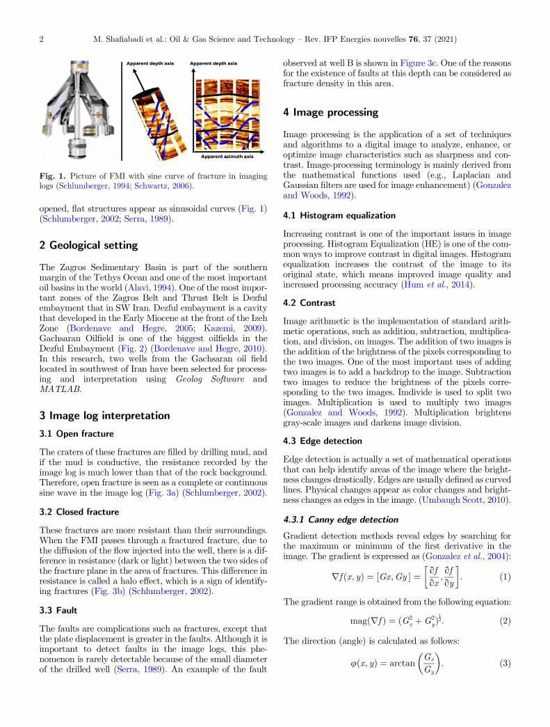
The Zagros Sedimentary Basin is part of the southernmargin of the Tethys Ocean and one of the most importantoil basins in the world (Alavi, 1994). One of the most impor-tant zones of the Zagros Belt and Thrust Belt is Dezfulembayment that in SW Iran. Dezful embayment is a cavitythat developed in the Early Miocene at the front of the IzehZone (Bordenave and Hegre, 2005; Kazemi, 2009).Gachsaran Oilfield is one of the biggest oilfields in theDezful Embayment (Fig. 2) (Bordenave and Hegre, 2010).In this research, two wells from the Gachsaran oil fieldlocated in southwest of Iran have been selected for process-ing and interpretation using Geolog Software andMATLAB.

3 Image log interpretation

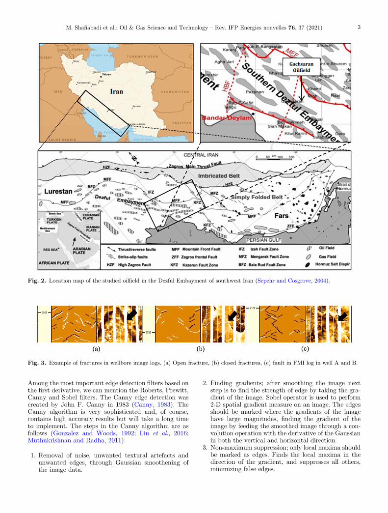
3.1 Open fracture

The craters of these fractures are filled by drilling mud, andif the mud is conductive, the resistance recorded by theimage log is much lower than that of the rock background.Therefore, open fracture is seen as a complete or continuoussine wave in the image log (Fig. 3a) (Schlumberger, 2002).

3.2 Closed fracture

These fractures are more resistant than their surroundings.When the FMI passes through a fractured fracture, due tothe diffusion of the flow injected into the well, there is a dif-ference in resistance (dark or light) between the two sides ofthe fracture plane in the area of fractures. This difference inresistance is called a halo effect, which is a sign of identify-ing fractures (Fig. 3b) (Schlumberger, 2002).

3.3 Fault

The faults are complications such as fractures, except thatthe plate displacement is greater in the faults. Although it isimportant to detect faults in the image logs, this phe-nomenon is rarely detectable because of the small diameterof the drilled well (Serra, 1989). An example of the fault

observed at well B is shown in Figure 3c. One of the reasonsfor the existence of faults at this depth can be considered asfracture density in this area.

4 Image processing

Image processing is the application of a set of techniquesand algorithms to a digital image to analyze, enhance, oroptimize image characteristics such as sharpness and con-trast. Image-processing terminology is mainly derived fromthe mathematical functions used (e.g., Laplacian andGaussian filters are used for image enhancement) (Gonzalezand Woods, 1992).

4.1 Histogram equalization

Increasing contrast is one of the important issues in imageprocessing. Histogram Equalization (HE) is one of the com-mon ways to improve contrast in digital images. Histogramequalization increases the contrast of the image to itsoriginal state, which means improved image quality andincreased processing accuracy (Hum et al., 2014).

4.2 Contrast

Image arithmetic is the implementation of standard arith-metic operations, such as addition, subtraction, multiplica-tion, and division, on images. The addition of two images isthe addition of the brightness of the pixels corresponding tothe two images. One of the most important uses of addingtwo images is to add a backdrop to the image. Subtractiontwo images to reduce the brightness of the pixels corre-sponding to the two images. Imdivide is used to split twoimages. Multiplication is used to multiply two images(Gonzalez and Woods, 1992). Multiplication brightensgray-scale images and darkens image division.

4.3 Edge detection

Edge detection is actually a set of mathematical operationsthat can help identify areas of the image where the bright-ness changes drastically. Edges are usually defined as curvedlines. Physical changes appear as color changes and bright-ness changes as edges in the image. (Umbaugh Scott, 2010).

4.3.1 Canny edge detection

Gradient detection methods reveal edges by searching forthe maximum or minimum of the first derivative in theimage. The gradient is expressed as (Gonzalez et al., 2004):

rf x; yð Þ ¼ Gx;Gy½ � ¼ ofox

;ofoy

� �: ð1Þ

The gradient range is obtained from the following equation:

mag rfð Þ ¼ ðG2x þG2

yÞ12: ð2Þ

The direction (angle) is calculated as follows:

u x; yð Þ ¼ arctanGx

Gy

� �: ð3Þ

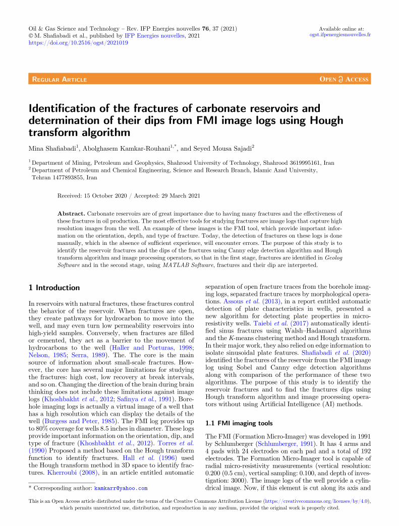
Fig. 1. Picture of FMI with sine curve of fracture in imaginglogs (Schlumberger, 1994; Schwartz, 2006).

M. Shafiabadi et al.: Oil & Gas Science and Technology – Rev. IFP Energies nouvelles 76, 37 (2021)2

Among the most important edge detection filters based onthe first derivative, we can mention the Roberts, Prewitt,Canny and Sobel filters. The Canny edge detection wascreated by John F. Canny in 1983 (Canny, 1983). TheCanny algorithm is very sophisticated and, of course,contains high accuracy results but will take a long timeto implement. The steps in the Canny algorithm are asfollows (Gonzalez and Woods, 1992; Liu et al., 2016;Muthukrishnan and Radha, 2011):

1. Removal of noise, unwanted textural artefacts andunwanted edges, through Gaussian smoothening ofthe image data.

2. Finding gradients; after smoothing the image nextstep is to find the strength of edge by taking the gra-dient of the image. Sobel operator is used to perform2-D spatial gradient measure on an image. The edgesshould be marked where the gradients of the imagehave large magnitudes, finding the gradient of theimage by feeding the smoothed image through a con-volution operation with the derivative of the Gaussianin both the vertical and horizontal direction.

3. Non-maximum suppression; only local maxima shouldbe marked as edges. Finds the local maxima in thedirection of the gradient, and suppresses all others,minimizing false edges.

Fig. 3. Example of fractures in wellbore image logs. (a) Open fracture, (b) closed fractures, (c) fault in FMI log in well A and B.

Fig. 2. Location map of the studied oilfield in the Dezful Embayment of southwest Iran (Sepehr and Cosgrove, 2004).

M. Shafiabadi et al.: Oil & Gas Science and Technology – Rev. IFP Energies nouvelles 76, 37 (2021) 3

4. Double threshold. Potential edges are determined bythresholding, instead of using a single static thresholdvalue for the entire image, the Canny algorithm intro-duced hysteresis thresholding, which has some adap-tively to the local content of the image. There aretwo threshold levels, th, high and tl, low whereth > tl. Pixel values above the th value are immedi-ately classified as edges.

5. Edge tracking by hysteresis. Final edges are deter-mined by suppressing all edges that are not connectedto a very strong edge.

The lower the threshold, the more lines become detect-able, on the other hand a high threshold may lose weak linesor parts of the lines. r plays the role of a scale parameter forthe edges. Large values of r produce coarser scale edges andsmall values of r produce finer scale edges. Larger values ofr also result in greater noise suppression. This r should notbe confused with standard deviation (Huang and Wang,2008).

4.4 Hough transform

The Hough transform invented by Richard Duda and PeterHart in 1972 (Duda and Hart, 1972). The Hough transformis a way of extracting features in image analysis, computervision, and digital image processing (Duda and Hart, 1972;Gonzalez et al., 2004). Since the boundaries are determinedat the edge detection stage, the exact shape of the edgesegments that correspond to fractures are found usingpattern recognition in order to characterize these curvesfully. The Hough transform is an established method fordetecting complex patterns of points in binary image data,and has been known to perform well in the presence ofnoise, extraneous data and occlusions (Illingworth andKittler, 1988). This edge description is commonly obtainedfrom a feature detecting operator such as the Roberts Cross,Sobel or Canny edge detector and may be noisy, i.e. it maycontain multiple edge fragments corresponding to a singlewhole feature. The idea of the Hough transform is, thatevery edge point in the edge map is transformed to allpossible lines that could pass through that point (Fig. 4).After applying the edge detection algorithm and gettingthe final results, the next step is to use the Houghalgorithm. The input image in the Hough algorithm is thecolored image (RGB) obtained from the result of the Cannyedge detection algorithm.

4.5 Curve fitting

Curve fitting is the process of constructing a curve, or math-ematical function, that has the best fit to a series of datapoints (Fig. 5). Most commonly, one fits a function of theform y = f(x) (Kolb, 1984).

4.6 Find dip of fractures

The dip is an angle that can have any value between0 (horizontal plane) to 90� (vertical plane) (Aguilera,2010). Figure 6 shows how to calculate the dip from thesinusoidal curves in the FMI Log.

5 Discussion and results

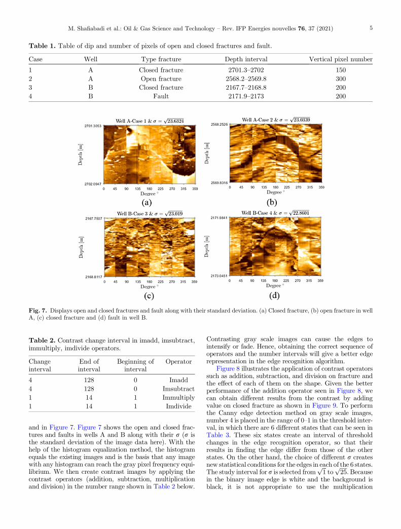
The field of study consists of FMI images of two wells Aand B, for which there are two sections selected from eachwell. More information on these sections is given in Table 1

Fig. 4. Represents a line in image space as a point in Houghspace (Wang and Wang, 2018).

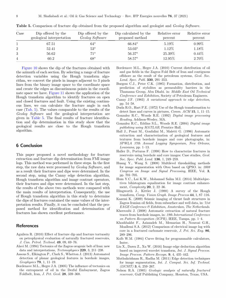
Fig. 5. Apply the Hough algorithm on the detected edge of theclosed fracture in well A.

Fig. 6. Sinusoidal curve dip calculation method in FMI imageslog. Dip angle = arc tan (h/d) where h = height of sinusoid andd = borehole diameter (Serra, 1989).

M. Shafiabadi et al.: Oil & Gas Science and Technology – Rev. IFP Energies nouvelles 76, 37 (2021)4

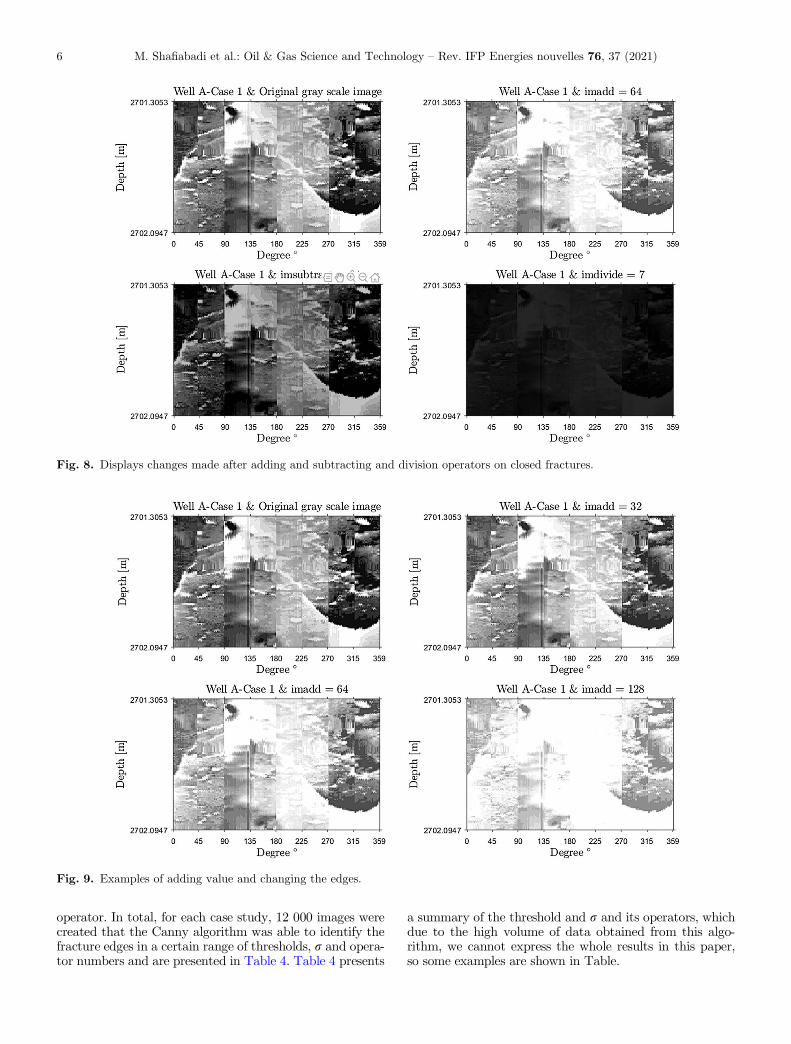
and in Figure 7. Figure 7 shows the open and closed frac-tures and faults in wells A and B along with their r (r isthe standard deviation of the image data here). With thehelp of the histogram equalization method, the histogramequals the existing images and is the basis that any imagewith any histogram can reach the gray pixel frequency equi-librium. We then create contrast images by applying thecontrast operators (addition, subtraction, multiplicationand division) in the number range shown in Table 2 below.

Contrasting gray scale images can cause the edges tointensify or fade. Hence, obtaining the correct sequence ofoperators and the number intervals will give a better edgerepresentation in the edge recognition algorithm.

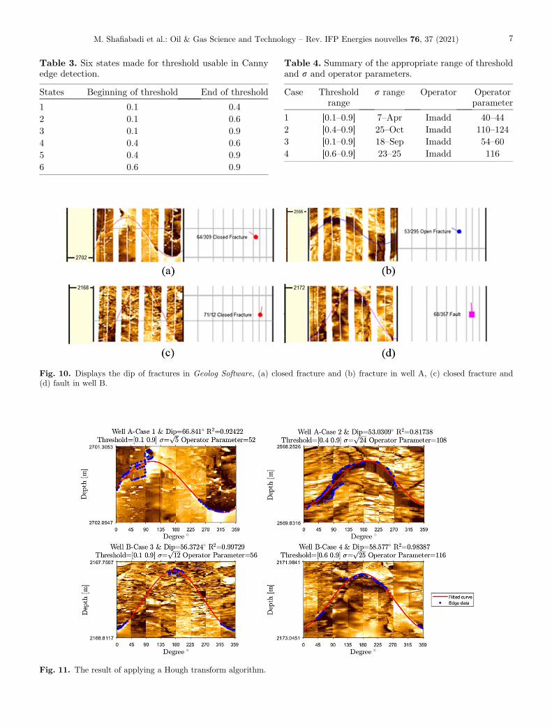
Figure 8 illustrates the application of contrast operatorssuch as addition, subtraction, and division on fracture andthe effect of each of them on the shape. Given the betterperformance of the addition operator seen in Figure 8, wecan obtain different results from the contrast by addingvalue on closed fracture as shown in Figure 9. To performthe Canny edge detection method on gray scale images,number 4 is placed in the range of 0–1 in the threshold inter-val, in which there are 6 different states that can be seen inTable 3. These six states create an interval of thresholdchanges in the edge recognition operator, so that theirresults in finding the edge differ from those of the otherstates. On the other hand, the choice of different r createsnew statistical conditions for the edges in each of the 6 states.The study interval for r is selected from

ffiffiffi1

pto

ffiffiffiffiffi25

p. Because

in the binary image edge is white and the background isblack, it is not appropriate to use the multiplication

Table 1. Table of dip and number of pixels of open and closed fractures and fault.

Case Well Type fracture Depth interval Vertical pixel number

1 A Closed fracture 2701.3–2702 1502 A Open fracture 2568.2–2569.8 3003 B Closed fracture 2167.7–2168.8 2004 B Fault 2171.9–2173 200

Fig. 7. Displays open and closed fractures and fault along with their standard deviation. (a) Closed fracture, (b) open fracture in wellA, (c) closed fracture and (d) fault in well B.

Table 2. Contrast change interval in imadd, imsubtract,immultiply, imdivide operators.

Changeinterval

End ofinterval

Beginning ofinterval

Operator

4 128 0 Imadd4 128 0 Imsubtract1 14 1 Immultiply1 14 1 Imdivide

M. Shafiabadi et al.: Oil & Gas Science and Technology – Rev. IFP Energies nouvelles 76, 37 (2021) 5

operator. In total, for each case study, 12 000 images werecreated that the Canny algorithm was able to identify thefracture edges in a certain range of thresholds, r and opera-tor numbers and are presented in Table 4. Table 4 presents

a summary of the threshold and r and its operators, whichdue to the high volume of data obtained from this algo-rithm, we cannot express the whole results in this paper,so some examples are shown in Table.

Fig. 8. Displays changes made after adding and subtracting and division operators on closed fractures.

Fig. 9. Examples of adding value and changing the edges.

M. Shafiabadi et al.: Oil & Gas Science and Technology – Rev. IFP Energies nouvelles 76, 37 (2021)6

Table 4. Summary of the appropriate range of thresholdand r and operator parameters.

Case Thresholdrange

r range Operator Operatorparameter

1 [0.1–0.9] 7–Apr Imadd 40–442 [0.4–0.9] 25–Oct Imadd 110–1243 [0.1–0.9] 18–Sep Imadd 54–604 [0.6–0.9] 23–25 Imadd 116

Fig. 10. Displays the dip of fractures in Geolog Software, (a) closed fracture and (b) fracture in well A, (c) closed fracture and(d) fault in well B.

Table 3. Six states made for threshold usable in Cannyedge detection.

States Beginning of threshold End of threshold

1 0.1 0.42 0.1 0.63 0.1 0.94 0.4 0.65 0.4 0.96 0.6 0.9

Fig. 11. The result of applying a Hough transform algorithm.

M. Shafiabadi et al.: Oil & Gas Science and Technology – Rev. IFP Energies nouvelles 76, 37 (2021) 7

Figure 10 shows the dip of the fractures obtained withthe azimuth of each section. By selecting a range of fracturedetection variables using the Hough transform algo-rithm, we convert the pixels in images adjacent to 3 pixelslines from the binary image space to the coordinate spaceand create the edges as discontinuous points in the coordi-nate space we have. Figure 11 shows the application of theHough transform algorithm to identify fractures on openand closed fractures and fault. Using the existing continu-ous lines, we can calculate the fracture angle in eachcase (Tab. 5). The values comparable to the results of theGeolog Software and the geological interpretation aregiven in Table 5. The final results of fracture identifica-tion and dip determination in this study show that thegeological results are close to the Hough transformalgorithm.

6 Conclusion

This paper proposed a novel methodology for fractureextraction and fracture dip determination from FMI imagelogs. This method was performed in three steps. In the firststep, the raw data were processed by Geolog Software, andas a result their fractures and dips were determined. In thesecond step, using the Canny edge detection algorithm,Hough transform algorithm and image contrast operators,their fractures and dips were determined. In the last step,the results of the above two methods were compared withthe main results of interpretation. Consequently, the useof Hough transform algorithm in this study to determinethe dips of fractures contained the same values of the inter-pretation results. Finally, it can be concluded that the pro-posed method for identification and determination offractures has shown excellent performance.

References

Aguilera R. (2010) Effect of fracture dip and fracture tortuosityon petrophysical evaluation of naturally fractured reservoirs,J. Can. Petrol. Technol. 49, 09, 69–76.

Alavi M. (1994) Tectonics of the Zagros orogenic belt of Iran: newdata and interpretations, Tectonophysics 229, 3, 211–238.

Assous S., Elkington P., Clark S., Whetton J. (2013) Automateddetection of planar geological features in borehole images,Geophysics 79, 1, 11–19.

Bordenave M.L., Hegre J.A. (2005) The influence of tectonics onthe entrapment of oil in the Dezful Embayment, ZagrosFoldbelt, Iran, J. Pet. Geol. 28, 339–368.

Bordenave M.L., Hegre J.A. (2010) Current distribution of oiland gas fields in the Zagros Fold Belt of Iran and contiguousoffshore as the result of the petroleum systems, Geol. Soc.Lond. Spec. Publ. 330, 291–353.

Burgess C.J., Peter C.K. (1985) Formation, distribution, andprediction of stylolites as permeability barriers in theThamama Group, Abu Dhabi. in: Middle East Oil TechnicalConference and Exhibition, Society of Petroleum Engineers.

Canny J.F. (1983) A variational approach to edge detection,pp. 54–58.

Duda R.O., Hart P.E. (1972) Use of the Hough transformation todetect lines and curves in pictures, Comm. ACM 15, 1, 11–15.

Gonzalez R.C., Woods R.E. (1992) Digital image processingReading, Addison-Wesley, MA.

Gonzalez R.C., Eddins S.L., Woods R.E. (2004) Digital imagepublishing using MATLAB, Prentice Hall.

Hall J., Ponzi M., Gonfalini M., Maletti G. (1996) Automaticextraction and characterization of geological features andtextures from borehole images and core photographs, in:SPWLA 37th Annual Logging Symposium, New Orleans,Louisiana, pp. 1–13.

Haller D., Porturas F. (1998) How to characterize fractures inreservoirs using borehole and core images: Case studies, Geol.Soc. Spec. Publ. Lond. 136, 1, 249–259.

Huang Y., Wang S. (2008) Multilevel thresholding methodsfor image segmentation with Otsu based on QPSO. in: 2008Congress on Image and Signal Processing, IEEE, Vol. 3,pp. 701–705.

Hum Y.C., Lai K.W., Mohamad Salim M.I. (2014) Multiobjec-tives bihistogram equalization for image contrast enhance-ment, Complexity 20, 2, 22–36.

Illingworth J., Kittler J. (1988) A survey of the Houghtransform, Comp. Vision Graph. Image Process 44, 1, 87–116.

Kazemi K. (2009) Seismic imaging of thrust fault structures inZagros Iranian oil fields, from subsurface and well data, in: 71stEAGE Conference & Exhibition, Amsterdam, The Netherlands.

Kherroubi J. (2008) Automatic extraction of natural fracturetraces from borehole images, in: 19th International Conferenceon Pattern Recognition (ICPR), IEEE, Tampa, pp. 1–4.

Khoshbakht F., Azizzadeh M., Memarian H., Nourozi G.H.,Moallemi S.A. (2012) Comparison of electrical image log withcore in a fractured carbonate reservoir, J. Pet. Sci. Eng. 86,289–296.

Kolb W.M. (1984) Curve fitting for programmable calculators,Imtec.

Liu X., Dawn Z., Xu W. (2016) Image edge deduction algorithmbased on improved wavelet transform, Int. J. Signal Process.Image Process. Pattern Recogn. 9, 4, 435–442.

Muthukrishnan R., Radha M. (2011) Edge detection techniquesfor image segmentation, Int. J. Comput. Sci. Inf. Technol.(IJCSIT) 3, 6, 259–267.

Nelson R.A. (1985) Geologic analysis of naturally fracturedreservoir, Gulf Publishing Company, Houston, Texas, USA.

Table 5. Comparison of fracture dip obtained from the proposed algorithm and geologist and Geolog Software.

Case Dip offered by thegeological interpretation

Dip offered by theGeolog Software

Dip calculated by theproposed method

Relative errorpercent

Relative errorpercent

1 67.51 64� 66.84� 5.19% 0.99%2 52.41 53� 53.03� 1.12% 1.18%3 56.62 71� 56.37� 25.39% 0.44%4 60.2 68� 58.57� 12.95% 2.70%

M. Shafiabadi et al.: Oil & Gas Science and Technology – Rev. IFP Energies nouvelles 76, 37 (2021)8

Safinya K.A., Lan P.L., Villegas M., Cheung P.S. (1991)Improved formation imaging with extended microelectricalarrays, Soc. Pet. Eng. 22726, 653–664.

Schlumberger (1991) Log Interpretation Principles/Applications,Schlumberger Educational Services.

Schlumberger (1994) FMI fullbore formation microimager,Schlumberger Educational Services, Houston, Texas.

Schlumberger (2002) FMI: borehole geology, geomechanics and3-D reservoir modeling. http://www.slb.com/media/services/evaluation/geology/fmi.pdf.

Schwartz B.C. (2006) Fracture pattern characterization of theTensleep Formation, Teapot Dome, Wyoming, Master Thesis,Department of Geology and Geography Morgantown, WestVirginia, pp. 115–130.

Sepehr M., Cosgrove J.W. (2004) Structural framework of theZagros Fold-Thrust Belt, Iran,Mar. Pet. Geol. 21, 7, 829–843.

Serra O. (1989) Formation microscanner image interpretation,Schlumberger Education Services, Houston, TX.

Shafiabadi M., Kamkar-Rouhani A., Ghavami Riabi S.R.,Roshandel Kahoo A., Tokhmechi B. (2020) Identification of

reservoir fractures on FMI image logs using Canny and Sobeledge detection algorithms, Oil Gas Sci. Technol. - Rev. IFPEnergies nouvelles 76, 11. https://doi.org/10.2516/ogst/2020086.

Taiebi F., Akbarizadeh G.H., Farshidi E. (2017) Detection ofreservoir fractures in imaging logs using directional filtering,in: 2017 5th Iranian Joint Congress on Fuzzy and IntelligentSystems (CFIS), IEEE, pp. 150–154.

Torres D., Strickland R., Gianzero M. (1990) A new approachto determining dip and strike using borehole images, in:SPWLA 31th Annual Logging Symposium, Lafayette, Louisiana,pp. 1–20.

Umbaugh S.E. (2010) Digital image processing and analysis,human and computer vision applications with CVIP tools, 2ndedn., CRC Press, Boca Raton, FL. ISBN 978-1-4398-0205-2.

Wang G., Wang W. (2018) The research on edge detectionalgorithm of lane. EURASIP J. Image Video Process. 2018, 1,1–9.

M. Shafiabadi et al.: Oil & Gas Science and Technology – Rev. IFP Energies nouvelles 76, 37 (2021) 9