IZA DP No. 488 Identifying Human Capital Externalities: Theory with an Application to US Cities Antonio Ciccone Giovanni Peri DISCUSSION PAPER SERIES Forschungsinstitut zur Zukunft der Arbeit Institute for the Study of Labor April 2002
Transcript
IZA DP No. 488
Identifying Human Capital Externalities:Theory with an Application to US CitiesAntonio CicconeGiovanni Peri
DI
SC
US
SI
ON
PA
PE
R S
ER
IE
S
Forschungsinstitutzur Zukunft der ArbeitInstitute for the Studyof Labor
April 2002
Identifying Human Capital Externalities: Theory with an Application to US Cities
Antonio Ciccone Universitat Pompeu Fabra, CEPR and IZA, Bonn
This Discussion Paper is issued within the framework of IZA’s research area Mobility and Flexibility of Labor. Any opinions expressed here are those of the author(s) and not those of the institute. Research disseminated by IZA may include views on policy, but the institute itself takes no institutional policy positions. The Institute for the Study of Labor (IZA) in Bonn is a local and virtual international research center and a place of communication between science, politics and business. IZA is an independent, nonprofit limited liability company (Gesellschaft mit beschränkter Haftung) supported by the Deutsche Post AG. The center is associated with the University of Bonn and offers a stimulating research environment through its research networks, research support, and visitors and doctoral programs. IZA engages in (i) original and internationally competitive research in all fields of labor economics, (ii) development of policy concepts, and (iii) dissemination of research results and concepts to the interested public. The current research program deals with (1) mobility and flexibility of labor, (2) internationalization of labor markets, (3) welfare state and labor markets, (4) labor markets in transition countries, (5) the future of labor, (6) evaluation of labor market policies and projects and (7) general labor economics. IZA Discussion Papers often represent preliminary work and are circulated to encourage discussion. Citation of such a paper should account for its provisional character. A revised version may be available on the IZA website (www.iza.org) or directly from the author.
Identifying Human Capital Externalities: Theory with an Application to US Cities�
Identification of the strength of human capital externalities at the aggregate level is still not fully understood. The existing method may yield positive or negative externalities even if wages reflect marginal social products. We propose an approach that yields positive average human capital externalities if and only if the marginal social product of workers with above-average human capital exceeds their wage. As an application, we estimate the strength of average-schooling externalities in US cities between 1970 and 1990. JEL Classification: O0, O4, R0, J3 Keywords: marginal social product of human capital, wages, human capital externalities,
imperfect substitution, perfect substitution, cities Antonio Ciccone Department of Economics and Business Universitat Pompeu Fabra Ramon Trias Fargas 25-27 08005 Barcelona Spain Tel.: +34-935 42 16 69 Fax: +34-935 42 17 46 Email: [email protected]
� We thank David Card for help with the data, Douglas Almond for excellent research assistance, and Daron Acemoglu, Orazio Attanasio, Joshua Angrist, Richard Blundell, Ken Chay, Adriana Kugler, Costas Meghir, Jonathan Temple, and Gianluca Violante for comments. Daron Acemoglu and Joshua Angrist kindly made their data and programs available to us. The theoretical results on identification in this paper were in part contained in two previous working papers, “Human Capital and Externalities in Cities,” (CEPR Discussion Paper No. 2599, 2000) by Ciccone and Peri and “Capital, Wages, and Growth: Theory and Evidence” by Ciccone, Peri, and Almond (CEPR Discussion Paper 2199, 1999). Ciccone thanks the Commission on Research at UC Berkeley (1997-1998), the Spanish Ministry of Education (1997-1999), and CREI for financial support for this project.
Human capital externalities at the aggregate level play a central role in applied economic
theory as well as economic policy analysis. In applied theory, human capital externalities are
invoked to capture key features of the data (e.g. Lucas (1988), Azariadis and Drazen
(1990), Black and Henderson (1999)). In policy analysis, the strength of human capital
externalities is one of the main determinants of the optimal subsidy to human capital (e.g.
Gemmell (1997), Heckman and Klenow (1998), Heckman (2000)). Assessing the strength
of human capital externalities at the aggregate level is therefore important for economic
theory as well as policy, and empirical research has responded with a variety of different
approaches and estimates (e.g. Rauch (1993), Conley, Flier, and Tsang (1999), Acemoglu
and Angrist (2000), Moretti (2000), Rudd (2000)). The theoretical identification problem is
still not fully understood however. The difficulty is simple to explain. Empirical work finds
that workers with different levels of education are imperfect substitutes in production (e.g.
Katz and Murphy (1992), Johnson (1997), Topel (1997), Autor, Katz, and Krueger (1998),
Card and Lemieux (2000)). An increase in the aggregate supply of highly educated workers
will therefore tend to increase wages of workers with low levels of education and decrease
wages of workers with high levels of education, even if wages of highly educated workers
reflect their marginal social product (and there is no need for corrective policies). Can we
avoid mistaking these standard supply effects with (positive or negative) human capital
externalities at the aggregate level?
So far the answer to this question is unclear as existing work on the estimation of the
strength of human capital externalities at the aggregate level assumes that workers with
different human capital are perfect substitutes in production. Perfect substitutability
simplifies the theoretical identification problem because it implies that the aggregate supply
of human capital does not affect individual wages if there are no externalities. All effects of
the supply of human capital on individual wages can therefore be interpreted as
externalities. This yields, for example, that average-schooling externalities at the local
geographic level can be estimated by simply including average schooling of the local
workforce in a standard Mincerian wage regression (e.g. Rauch (1993), Acemoglu and
Angrist (2000), Rudd (2000)). It can be shown however that if workers with different levels
of education are imperfect substitutes in production then this (Mincerian) approach to
human capital externalities at the aggregate level may yield positive or negative externalities
even if wages reflect marginal social products.
2
We therefore propose an approach to the identification of human capital externalities at
the aggregate level that is theoretically valid whether workers with different human capital
are perfect or imperfect substitutes in production. The approach can be applied at the city-
level, the region-level, or (with some modifications that will be explained later) the country-
level. The theoretical basis of the approach at the local geographic level is that if wages
( )w Z of workers with skills Z reflect marginal social products then changes in the average
level of human capital of the local workforce have no first-order effect on average wages
( ) ( )Zw w Z l Z= ∑ when workforce skill-composition weights ( )l Z are held constant.1 If
wages of high-skilled workers are below their marginal social product however then there
will be a positive first-order effect of average human capital at the aggregate level on
average wages even when workforce skill-composition is held constant.
To get some intuition of how this theoretical argument applies to average-schooling
externalities at the city-level, consider a city experiencing an inflow of highly educated
workers resulting in a small increase in average schooling and hence productivity (we will
deal with large increases later). For simplicity, assume that output is produced without
physical capital and land. Suppose also that workers with different levels of education are
imperfect substitutes in production and that there are no city-level average-schooling
externalities (wages reflect marginal social products). In this case, incoming workers,
through their effect on the supply of different levels of education in the city, raise the wage
for some levels of education and lower it for others. But because they are paid their
marginal social product, incoming workers will not affect total wage income of the group of
workers who already were in the city before the human capital inflow. Assuming for
simplicity that productivity does not depend on the aggregate scale of production (we will
account for possible scale effects later), this implies that average wages using the city’s
workforce skill-composition before the human capital inflow will be the same before and
after the increase in average schooling. Now suppose instead that there are positive city-
level average-schooling externalities. Wages of incoming, highly educated workers will in
this case be lower than their marginal social product and some of the increase in aggregate
production will go to the group of workers who already were in the city before the human
capital inflow. The inflow of human capital therefore increases average wages even when
workforce skill-composition is held constant.
1 But changes in the average level of human capital of the local workforce will have a first-ordereffect on wages of workers with particular skills if workers with different human capital areimperfect substitutes in production
3
The theoretical setting that we employ to discuss identification of human capital
externalities at the aggregate level is based on the human capital framework used in most
theoretical and empirical work at the aggregate level involving human capital.2 This
framework yields a parsimonious way of capturing imperfect substitutability among workers
with many different levels of human capital.3 Moreover, the framework is easily extended to
allow for human capital externalities and encompasses the Mincerian approach to externa-
lities.4 Our main theoretical result regarding identification of human capital externalities at
the aggregate level is that the partial elasticity of average wages with respect to average
human capital is equal to the strength of average human capital externalities when
workforce skill-composition weights are held constant. This result, which holds whether
workers with different human capital are perfect or imperfect substitutes in production, is
the basis of what we call the constant-composition approach to the identification of human
capital externalities at the aggregate level. We also analyze second-order effects of average
human capital on average wages holding workforce skill-composition constant.
Furthermore, we show that the constant-composition approach can be used to identify
human capital externalities that are biased towards workers with high or low levels of
human capital.
As an application of the constant-composition approach, we assess the strength of
average-schooling externalities in 163 US cities between 1970 and 1990 using instrumental-
variable estimation methods to account for endogenous changes in schooling. Our results
yield no evidence of significant average-schooling externalities. This finding depends
critically on the constant-composition approach being flexible enough for workers with
different human capital to be imperfect substitutes in production. Imposing perfect
substitutability and using the Mincerian approach with the same data and instruments yields
2 E.g. Lucas (1988), Mankiw, Romer, and Weil (1992), Benhabib and Spiegel (1994), Klenow andRodriguez-Clare (1997), Hall and Jones (1999), Topel (1999), Bils and Klenow (2001), de la Fuenteand Domenech (2001), Krueger and Lindahl (2001), and Temple (2001).3 The framework used by Katz and Murphy (1992) captures imperfect substitutability amongworkers with many different levels of education in an equally parsimonious way. The twoframeworks are closely related and our identification results carry over directly to the KMframework. The proofs are only a matter of appropriate relabeling. The KM framework does notencompass the Mincerian approach to human capital externalities however.4 Another framework is the constant-elasticity-of-substitution model used by Moretti (2000). Thetwo main drawbacks of this framework are the assumption that the elasticity of substitution betweenworkers with different schooling is the same whether schooling is very similar or very different andthat it is unclear how the strength of average-schooling externalities can be identified.
4
that a one-year increase in average schooling has a (statistically significant) external effect
on productivity of at least 7 percent.
It is well known that wages are in part determined by skills that are unobservable to
empirical researchers. This raises the question of how our approach to average-schooling
externalities is affected by workers with high wages due to unobservable characteristics
(e.g. ability) moving into cities that experience rapidly increasing levels of average
schooling. Our data allow us to distinguish between individuals who have worked for a
longer period in a city and individuals who moved into the city recently. Hence, we can
estimate the wage-differential between “movers” and “stayers” conditional on observable
characteristics like education and experience. Our empirical results indicate that this mover-
stayer wage-differential is positively correlated with the increase in average schooling in
cities between 1970 and 1990 for most education levels. This provides support for the view
that cities experiencing rapidly increasing levels of average schooling attract workers with
higher ability and that least-squares estimates of average-schooling externalities at the city-
level may be biased upwards for this reason. Mover-stayer wage-differentials are not
significantly correlated with the increase in average schooling predicted by our instruments
for most education levels however. The only exception is the wage-differential for the group
of workers with 9 to 12 years of schooling, which is positively correlated with the predicted
increase in average schooling. This suggests that our instrumental-variable estimates may
understate the strength of average-schooling externalities but are unlikely to overstate them.
The variables used as instruments for the change in average schooling between 1970
and 1990 are the city-level demographic structure of the workforce and population as well
as the population-share of African-Americans, all in 1970, and various interaction terms.
These variables have predictive power for the change in average schooling at the city-level
because younger individuals entering the labor force during this time period had higher
levels of schooling than workers going into retirement and because African-Americans were
rapidly catching-up in schooling levels with the rest of the population. Our identifying
hypothesis is that the variables used as instruments affect aggregate productivity growth
between 1970 and 1990 at the city-level only through the change in schooling and other
explanatory variables included in the estimating equation. We check this hypothesis by
testing the implied overidentifying restrictions (as well as by including selected instruments
directly into the estimating equation) and find it cannot be rejected at standard significance
levels. As a further check on the instruments, we use them to estimate the strength of
average-schooling externalities between 1970 and 1990 at the US state-level and compare
5
the result to estimates obtained with the state-level compulsory-schooling and child-labor-
law instruments used by Acemoglu and Angrist (2000). The two sets of instruments yield
basically identical estimates.
Mincerian wage regressions to estimate average-schooling externalities in cities were
introduced by Rauch (1993). Assuming that average schooling across cities is exogenous,
he finds statistically significant externalities in a cross-section of 237 cities in 1980.
Acemoglu and Angrist (2000) use the Mincerian approach to estimate average-schooling
externalities at the US state-level, accounting for state-specific fixed effects and
endogeneity of average and individual schooling. Their instrumental-variable approach,
which exploits differences in compulsory-schooling and child-labor laws across states and
over time, yields no evidence for significant average-schooling externalities. Rudd (2000)
also implements the Mincerian approach at the US state-level, allowing for state-specific
fixed effects and controlling for a variety of state-level variables that may affect wages, and
like Acemoglu and Angrist does not find evidence for average-schooling externalities.
Moretti (2000) accounts for endogenous supply when estimating externalities to the share
of college-educated workers in US cities. His theoretical framework allows for imperfect
substitutability of workers with different human capital in production but cannot be used to
estimate the strength of externalities.5 Conley, Flier, and Tsang (1999) report significant
instrumental-variable estimates of aggregate human capital externalities in Malaysian
regions. The main difference between these papers and our work is that we show how the
strength of average human capital externalities can be identified when workers with
different human capital are imperfect substitutes in production. There appears to be no
previous work on the identification of biased human capital externalities.
The remainder of the paper is organized in the following way. Section 2 presents the
theoretical framework. Section 3 derives the main theoretical results on the identification of
human capital externalities at the aggregate level. Section 4 contains the estimating
equations and explains the estimation methods used. Section 5 describes the data and
discusses the instruments. Section 6 presents our empirical results and section 7
summarizes.
5 Moretti argues that his framework yields qualitative evidence for externalities however. Theargument is based on his finding that wages of college-educated workers at the city-level increasewith their share in the workforce. This result is difficult to interpret however as he ignores aggregatescale effects and does not control for the relative supply of other, possibly complementary, types ofworkers.
6
2 The Human Capital Framework with Externalities
We now present the aggregate human capital framework with externalities and discuss the
identification problem raised by imperfect substitutability between workers with different
levels of human capital. The model is the simplest version of the framework that allows us
to discuss this identification problem. Extensions will be discussed later. The geographical
units of analysis are taken to be cities.
2.1 Model
Assume that output Y of each city depends on the aggregate amount of labor L and human
capital H employed in the city according to the following production function
( , )Y AF L H= , (1)
where A denotes the level of total factor productivity (TFP) in the city and H is
0
( )H xL x dx∞
≡ ∫ , (2)
where ( )L x is the number of workers with human capital x in the city (using this notation
the aggregate amount of labor in the city is ( )L L x dx≡ ∫ ). Assume also that the aggregate
production function is twice continuously differentiable and subject to constant returns to
scale to labor ( )L x for all x (or, alternatively, subject to constant returns to scale to L , H )
as well as constant or decreasing returns to human capital, 22 ( , ) 0F L H ≤ .
We will allow for the possibility that the marginal social product of workers with
above-average (below-average) human capital is greater (smaller) than their equilibrium
wage. This is accomplished by assuming that TFP may be increasing in the average level of
human capital /h H L= in the city and that this effect takes the form of an externality (e.g.
Lucas (1988)). The supply of human capital in the city will therefore affect aggregate
production by increasing output conditional on TFP as well as by increasing TFP. Only the
former effect will be reflected by wages in our theoretical framework.
To be more precise assume that firms in city c have access to the production function
in (1) and that they maximize profits taking the city-time specific levels of TFP as given.
Suppose also that product and labor markets are perfectly competitive and that output is
tradable. Under these assumptions the equilibrium product wage of workers with human
capital x in a city with average human capital h can be written as
( , ) ( ) ( )L Hw x h w h w h x= + , (3)
7
where Lw , Hw will be referred to as the price of labor and the price of human capital
respectively. The price of labor captures the equilibrium wage of workers without human
capital and the price of human capital the wage increase associated with an additional unit
of human capital. Both equilibrium prices are linked to TFP, the supply of labor, and the
supply of human capital in the city by the usual marginal productivity conditions
1( ) (1, )Lw h AF h= , (4)
2( ) (1, )Hw h AF h= , (5)
where we have used constant returns to scale of the production function given TFP.
Equation (3) implies that identical workers in the same city earn the same product
wage. Identical workers in different cities may earn different product wages in equilibrium
however as we assume that cities differ in characteristics that are relevant for workers’
utility. Examples of such characteristics are the cost of housing, the quality of public
schools, local tax-rates, the degree of air pollution, the crime rate, climate, outdoor
recreational opportunities, proximity to family or friends, and the variety or quality of
restaurants or sports teams. In this case, competitive labor markets imply that product
wages across cities satisfy ( ( ), )i
c cU w x z = ( ( ), )iU w x zκ κ for i I∈ and all , c κ , where , cz zκ
denote vectors of all characteristics of cities , c κ that are relevant for utility iU of type i
workers; i captures heterogeneity in preferences.
The specification used for TFP at the city-level is
A Dh Lθ δ= , (6)
where D stands for exogenous city-time specific factors affecting TFP and , h L are the
average level of human capital and aggregate employment in the city. The strength of
average human capital externalities is captured by the elasticity θ . Aggregate scale effects,
where scale is measured by aggregate employment, are captured by δ . Aggregate scale as a
determinant of productivity at the local geographic level is emphasized in Marshall (1890)
and Henderson (1988), and estimated in Sveikauskas (1975), Moomaw (1981), Henderson
(1986, 1988), Rauch (1993), and Ciccone and Hall (1996) for example. The specification in
(6) implies that the effect of an increase in the aggregate stock of human capital on TFP
depends in general on how much of the increase is due to aggregate employment growth
and how much is due to the growth of average human capital.
The model presented so far is the simplest framework that allows us to discuss
identification of human capital externalities when different levels of human capital may be
8
imperfect substitutes. It can be extended in several dimensions without affecting our
theoretical results on identification or our empirical approach. The most important
extension would include physical capital and land as factors of production. Extending the
theoretical and empirical work to allow for physical capital is simple when physical capital
moves to equalize its rate of return across the geographic units of analysis. Identifying
human capital externalities at the aggregate level when physical capital is not perfectly
mobile across the geographic units of analysis is also straightforward (this is the relevant
case for human capital externalities at the country-level). The main insight of extending the
theoretical analysis to allow for land as a factor of production is that the strength of
externalities will be identified net of congestion effects. All these extensions are discussed in
detail in the appendix. It may be worthwhile to point out that the model with land and
physical capital has many similarities with the theoretical work of Roback (1982). The
model can also be extended to allow for non-tradable goods and for “pecuniary”
externalities due to imperfect competition and increasing returns in the production of non-
tradables (e.g. Krugman (1992)). These extensions can also be found in the appendix. The
main conclusion of the first extension is that the constant-composition approach identifies
externalities in the tradable-goods sector only. The main conclusion of the second extension
is that the constant-composition approach can also be used to identify “pecuniary”
externalities.
2.2 Substitutability and Returns to Human Capital
The framework described so far is flexible enough to allow workers with different levels of
human capital to be perfect or imperfect substitutes in production. Perfect substitutability is
equivalent to constant returns to human capital given TFP. To see this notice that constant
(marginal) returns to human capital 22 (1, ) 0F h = imply that the production function in (1)
simplifies to( )Y A BL H= + (7)
where B is a (possibly city-time specific) exogenous variable. Hence, workers with different
human capital are perfect substitutes (the marginal rate of substitution between any two
different types of workers is independent of the proportion of the two types used in
production). Moreover, it is straightforward to show that perfect substitutability between
workers with different human capital combined with constant returns to scale given TFP
implies constant returns to human capital given TFP. Constant returns to human capital
given TFP and perfect substitutability between workers with different human capital are
therefore equivalent in the aggregate human capital framework. Constant returns to human
9
capital given TFP combined with (3) to (5) yields that the equilibrium wage schedule
simplifies to ( )w x AB Ax= + . Wages of workers with a given level of human capital and the
return to human capital will therefore be independent of the average level of human capital
in the city if TFP is held constant. Hence, all effects of the average level of human capital on
the equilibrium wage schedule must arise through TFP and can be interpreted as
externalities.
Imperfect substitutability between different types of workers in production on the other
hand is equivalent to decreasing (marginal) returns to human capital 22 (1, ) 0F h < . To see this
in a simple way suppose that the supply of workers with low human capital lx in a city
decreases while the supply of workers with high human capital hx ( )h lx x> increases so as
to keep the total number of workers constant. It can be shown that the implied change in
the relative wage of low human capital workers ( ) / ( )l hw x w x is proportional to2
22 (1, )( )h lF h x x− − in this case (this result is derived in detail in the appendix).6 Hence, the
decrease in the supply of low human capital workers and increase in the supply of high
human capital workers will increase the relative wage of low human capital workers if and
only if there are decreasing returns to human capital. Moreover, the implied increase in the
relative wage is smaller the closer lx to hx . This is because the closer the levels of human
capital of the two types of workers, the better they substitute for one another.
3 Identification of Human Capital Externalities
We first discuss the Mincerian approach to human capital externalities. Then we turn to the
constant-composition approach.
3.1 The Mincerian Approach
Suppose that aggregate production is subject to constant returns to human capital given
TFP and that human capital is essential in production. In this case the aggregate production
function in (1) simplifies to Y AH= and the equilibrium wage schedule at the city-level
defined in (3)-(5) can be written as log ( ) log logw x Dh L xθ δ= + using the formulation for
endogenous TFP in (6). Assume also that individual human capital is linked to individual
schooling s by exp( )x sγ= . In this case the equilibrium log-wage schedule becomes
6 If there are only two types of workers, the production function in (1) implies that the elasticity ofsubstitution between the two types is inversely proportional to 2
22 (1, )( )h lF h x x− − .
10
log ( ) log log logw s D L h sδ θ γ= + + + . (8)
The strength of average-schooling externalities ( log / )h Sθ ∂ ∂ can therefore be estimated as
the effect of average schooling in cities on the intercept of an individual (Mincerian) wage
regression or, using a city-specific fixed-effects approach, as the effect of changes in
average schooling in cities on changes of the intercept. This is the basis of the Mincerian
approach to schooling externalities in Rauch (1993), Acemoglu and Angrist (2000), and
Rudd (2000). The strength of aggregate scale effects δ can be estimated as the effect of
(changes in) log-employment on (changes in) the intercept.
To get a sense for the possible biases of the Mincerian approach when workers with
different levels of education are imperfect substitutes in production assume (without loss of
generality) that individual levels of human capital are linked to individual schooling s by
( ) exp( ( ))x s g s= . Log-linearizing the equilibrium wage schedule in (3) to (5) around the
average level of schooling S yields log ( )w s = log ( ) ( ) '( )( )w S S g S s Sβ+ − , where ( )w S is
the wage of workers with average schooling S and ( ) ( ) / ( )HS w x S w Sβ = the share of
human capital in the wage of workers with average schooling. The log-linearized
equilibrium wage schedule can therefore be written as
log ( ) log ( )w s w S RS Rs= − + . (9)
where ( ) '( )R S g Sβ= . There are two main differences between (8) and (9). First, the
individual return to schooling R may depend on the average level of human capital. Second,
making use of (3) to (5), the marginal effect of average schooling on the Mincerian
intercept is equal to
2 12 22
1 2 1 2
(1, ) ( ) (1, ) (1, ) ( )log'( )
(1, ) (1, ) ( ) (1, ) (1, ) ( )
F h x S F h F h x Sh h Rg S R S
S F h F h x S F h F h x S S Sθ
+∂ ∂ ∂+ + − −
∂ + + ∂ ∂ (10)
and may therefore not be equal to average-schooling externalities ( log / )h Sθ ∂ ∂ . Using
( ) '( )R S g Sβ= , 2 1 2( ) (1, ) ( ) /( (1, ) (1, ) ( ))S F h x S F h F h x Sβ = + and that twice continuous
differentiability and constant returns to scale given TFP of the production function in (1)
imply 12 22(1, ) (1, )F h F h h+ = 21 22(1, ) (1, ) 0F h F h h+ = , we obtain that the difference between the
marginal effect of average schooling on the Mincerian intercept and the strength of average-
schooling externalities is equal to
22
2
(1, )Bias of Mincerian Approach ( ( ) )
(1, )
R F h hS w S w
S AF h S
∂ ∂= − + − ∂ ∂
, (11)
11
where we also used that (3) and (5) imply that the difference between average human
capital and the human capital of the workers with average schooling can be written as
( )h x S− = ),1(/))(( 2 hAFSww − . Hence, the bias of the Mincerian approach to average-
schooling externalities when workers with different levels of human capital are imperfect
substitutes depends on two main factors. First, whether the individual return to schooling
increases or decreases with the average level of schooling. Second, whether the average
wage is greater or smaller than the wage of workers with the average level of schooling.
The main drawback of the Mincerian approach to human capital externalities at the
aggregate level is therefore that it yields biased estimates when workers with different
human capital are imperfect substitutes. Another drawback is its reliance on Mincerian wage
regressions. These regressions raise the concern of endogeneity and mismeasurement of
individual schooling and, more generally, correct econometric specification. Some of these
problems may be addressed by using instrumental-variable estimation methods (e.g.
Acemoglu and Angrist (2000)). But good instruments for individual schooling will usually
be unavailable at the local geographic level where externalities are often likely to be
strongest. For example, none of the usual instruments for individual schooling is available at
the level of US cities.
3.2 The Constant-Composition Approach
The main advantage of the constant-composition approach to the identification of human
capital externalities at the aggregate level compared to the Mincerian approach is that it is
theoretically valid whether workers with different education are perfect or imperfect
substitutes in production. Moreover, the approach does not require estimation of the return
to schooling at the individual level. These two results are demonstrated first. Then we turn
to second-order effects of average schooling on average wages holding the workforce
composition constant and apply the constant-composition approach to the case where
human capital externalities may be biased towards workers with high or low human capital.
3.2.1 Basic Constant-Composition Approach
The constant-composition approach is based on the theoretical result that the partial
elasticity of average wages with respect to average human capital holding workforce skill-
composition weights constant is equal to the strength of average human capital externalities
(whether workers with different levels of human capital are perfect or imperfect
substitutes). To prove this result notice that the average wage in a city can be written as
12
0
( , ( ) : 0) ( , ) ( )w h l x x w x h l x dx∞
≥ = ∫ . (12)
This notation emphasizes that average wages depend on individual wages of workers with
human capital x as well as workforce skill-composition weights ( ) ( ) /l x L x L= and that
individual wages depend on average human capital in the city. We can now state our main
theoretical result.
Proposition 1: The elasticity of the average wage with respect to the average level of
human capital yields the strength of average human capital externalities when workforce
skill-composition weights ( )l x are held constant
0 ( ) constant
( ) ( , ) ( , )( , )l x x
w h l x w x h w x h hdx
h w w h w x hθ
∞
∀
∂ ∂ = = ∂ ∂ ∫ . (13)
Proof: There are different ways to prove this result. One is to notice the relationship
between (13) and the dual approach to TFP accounting.7 But it is also possible to give a
proof that mirrors the intuitive explanation given in the introduction. Suppose that the
shares of workers with different human capital go from { }( ) : 0l x x ≥ to { }*( ) : 0l x x ≥ and
that the implied increase in average human capital is h∆ . Using the equilibrium wage
schedule in (3) and ignoring aggregate scale effects for simplicity yields that the average
wage holding workforce skill-composition constant increases by
( )0( ) ( ) ( ) (1, )L Hw h h w h h x l x dx Dh F hθ∞
+ ∆ + + ∆ −∫ . The first term can be written as
( ) ( )0 0( ) ( ) *( ) ( ) ( ) ( ( ) *( ))L H L Hw h h w h h x l x dx w h h w h h x l x l x dx
∞ ∞+ ∆ + + ∆ + + ∆ + + ∆ −∫ ∫ , the
average wage using the new workforce composition minus the increase in the average wage
due to the change in the workforce composition, which simplifies to
( ) (1, )D h h F h hθ+ ∆ + ∆ ( )Hw h h h− + ∆ ∆ . Hence, the percentage increase in the average wage
7 To see this notice that the equilibrium wage schedule in (3) implies that the left-hand side of (13) isequal to (1 )H Lβε β ε+ − , where ( / )( / )i i ih w w hε = ∂ ∂ for ,i L H= and β denotes the share ofhuman capital in the average wage, i.e. a weighted average of the elasticities of the price of labor andhuman capital with respect to average human capital with weights equal to the shares of labor andhuman capital in the average wage. The proof that this weighted average is equal to the strength ofaverage human capital externalities is very similar to the derivation of the dual approach to TFPaccounting. The only difference is that instead of considering the change in TFP associated with thepassing of time (dual TFP accounting) we consider the change in TFP associated with an increase inaverage human capital.
13
holding workforce skill-composition weights constant, relative to the percentage increase in
average human capital, becomes
( ) (1, ) (1, )(1, )
(1, ) (1, ) ( )(1, )
H
D h h F h h Dh F h hDh F h
hh
Dh F h h Dh F h w h h hDh F h
hh
θ θ
θ
θ θ
θ
+ ∆ + ∆ − + ∆
∆
+ ∆ − − + ∆ ∆
+∆
which simplifies to
1 1
(1, ) (1, )( )( ) (1, )
(1, ) (1, )
Hh DF h h h DF hw h hh h h DF h h h
h h DF h h DF h
θ θ
θ θ
θ θ− −
+ ∆ − − + ∆+ ∆ − + ∆ ∆+∆
.
As the increase in average human capital becomes small, the second term converges to an
expression that is proportional to the difference between the marginal product of human
capital given TFP and the price of human capital, 2 (1, ) ( )HDh F h w hθ − , which is zero in
equilibrium. The first term converges to θ , which is the strength of human capital
externalities. Q.E.D.
This proposition suggests that we can estimate the strength of average-schooling
externalities ( log / )h Sθ ∂ ∂ in cities between 1970 and 1990 in two steps. First, obtain the
average wage in 1990 in each city using the 1970 workforce composition,
1990 1990 1970( ) ( )Fc c cZw w Z l Z= ∑ where Z is the vector of all observable characteristics of
workers. Second, estimate the effect of the increase in average schooling in cities 1970-
1990, 1970 1990 1990 1970c c cS S S−∆ = − , on the log-change in wages holding workforce skill-
composition weights constant, 1970 1990 1990 1970log log logF Fc c cw w w−∆ = − .
Regarding the identification of aggregate scale effects, it is straightforward to show
that the strength of aggregate scale externalities δ is equal to the partial elasticity of
average wages (whether the workforce composition is held constant or not) with respect to
aggregate employment.
14
3.2.2 Second-Order Effects
So far we have concentrated on first-order effects of the average level of human capital on
average wages holding workforce skill-composition weights constant. We now turn to the
analysis of second-order effects. The next proposition proves that second-order effects are
always positive.
Proposition 2: Suppose that the aggregate production function in (1) is three times
continuously differentiable. Then the second-order effect of the log of average human
capital on the log of average wages when holding workforce skill-composition weights
constant is
0
222 (1, )
0(1, )
h h
F h h
F hσ
=
= − ≥ , (14)
where 0 ( )h l x xdx= ∫ . The quadratic approximation of the relationship between the log-
change of average wages holding workforce skill-composition weights constant and the log-
change of average human capital is therefore
2
( ) constant log ( , ( ) : 0) ( log ) ( log )
l x xw h l x x h hθ σ
∀∆ ≥ = ∆ + ∆ . (15)
Proof: The first order effect is
1 2 0 12 22 0
1 2 0
log( (1, ) (1, ) ) (1, ) (1, )
log (1, ) (1, )
F h F h h F h F h hh
h F h F h hθ θ
∂ + ++ = +
∂ +.
evaluated at 0h h= . The second-order effect can be obtained by differentiating the
expression above with respect to logh and evaluating at 0h h= . Differentiation yields
1 2 012 22 0
2122 222 0
1 2 0
(1, ) (1, )( (1, ) (1, ) )
(1, ) (1, )
(1, ) (1, )
h
F h F h hh F h F h h
h
F h F h hh
F h F h h
∂ + +
∂
+++
.
The first term evaluated at 0h h= is zero because constant returns to scale of the production
function given TFP implies that 2 ( , )F L H is homogenous of degree zero, which combined
15
with twice continuous differentiability of the production function yields
12 22 0 21 22 0(1, ) (1, ) (1, ) (1, ) 0F h F h h F h F h h+ = + = for 0h h= . To simplify the second term notice
that constant returns to scale given TFP also imply that 1 0 2 0 0 0(1, ) (1, ) (1, )F h F h h F h+ = and
that 22 ( , )F L H is homogenous of degree minus one. The latter combined with three times
continuous differentiability of the production function yields
22 0 221 0 222 0 0 122 0 222 0 0(1, ) (1, ) (1, ) (1, ) (1, )F h F h F h h F h F h h− = + = + . Hence, the second term evaluated
at 0h h= becomes 222 0 0 0(1, )( ) / (1, )F h h F h− . Q.E.D.
An immediate implication of (14) is that the second-order effect of average human capital
on average wages holding workforce skill-composition weights constant is zero if and only
if workers with different human capital are perfect substitutes (returns to human capital in
production are constant).
The intuition for this last proposition is simple. Suppose that human capital
externalities are absent and that returns to human capital are constant. In this case the
marginal social product of human capital does not depend on the average level of human
capital used in production. Hence, the price of human capital reflects the marginal social
product as well as the intra-marginal social product of human capital. Even a large increase
in average human capital will therefore not result in an increase in average wages holding
workforce skill-composition constant. In the case human capital externalities are absent and
the marginal product of human capital is strictly decreasing in the average level of human
capital used in production, however, the price of human capital reflects the marginal social
product of human capital but is below the intra-marginal social product of human capital.
Hence, a large increase in average human capital will result in an increase in average wages
holding workforce skill-composition constant (even if wages reflect marginal social
products).
When the production function in (1) is of the constant-elasticity-of-substitution type,
with the elasticity of substitution between labor and human capital equal to ε , the second-
order effect can be written as
(1 )β βσ
ε−
= , (16)
where β is the share of human capital in the average wage. This result will be useful later
when we assess the bias of the basic constant-composition approach to average-schooling
externalities when second-order effects are important but omitted in the estimating
equation.
16
3.2.3 Biased Human Capital Externalities
Our analysis so far has maintained that human capital externalities enter production in a
Hicks-neutral way. We now turn to the case where human capital externalities at the
aggregate level may be biased towards workers with high levels of human capital or
workers with low levels of human capital. To do so the aggregate production function in (1)
is replaced by
( , )L HY F A L A H= , (17)where
LLA Dhθ= and H
HA Dhθ= ; (18)
,L Hθ θ capture externalities of average human capital at the city-level. For simplicity it is
assumed that aggregate scale effects are absent. We also assume that the production
function is twice continuously differentiable and subject to constant returns to scale given
LA , HA as well as constant or decreasing returns to human capital given LA , HA ,
22 ( , ) 0L HF A L A H ≤ . The specification in (17) and (18) implies that human capital
externalities affect relative wages of workers with different human capital if L Hθ θ≠ and the
elasticity of substitution between L and H is different from unity.
To determine the strength of average human capital externalities implied by (17) and
(18) suppose that average human capital increases by one percent. The resulting increase in
average labor productivity is (1 ) (1 )L Hθ β θ β− + + where β is the share of human capital in
the average wage. Of this total increase, (1 )L Hθ β θ β− + is due to human capital
externalities and will be referred to as the strength of human capital externalities at the
aggregate level. The next proposition states that the strength of human capital externalities
when externalities may be biased can be identified with the constant-composition approach.
Proposition 3: Suppose that the aggregate production function is given by (17). Then the
elasticity of average wages with respect to average human capital holding workforce skill-
composition weights constant is equal to (1 )L Hθ β θ β− + .
Proof: The aggregate production function implies that the equilibrium wage schedule is
given by ( , ) L Hw x h w w h= + where the equilibrium prices of labor and human capital are
given by 1( , )L H LLw DF h L h H hθ θ θ= and 2( , )L H HHw DF h L h H hθ θ θ= . This equilibrium wage
schedule implies
17
( )0
1 2 0
( ) constant
log ( , ) ( , )
log
L H L L H H
l x xh h
DF h L h H h DF h L h H h hw h
h w h
θ θ θ θ θ θ
∀=
∂ +∂=
∂ ∂.
Constant returns to scale of the aggregate production function given LA and HA yields that
the marginal product of human capital is homogenous of degree zero. The right-hand-side
of the equation can therefore be written as
( )0
1 11 2 0
log (1, ) (1, )
log
H L L H L H
h h
DF h h DF h h h
h
θ θ θ θ θ θ+ − + −
=
∂ +
∂
( )0
0
1 112 22 0
0
(1 ) (1, ) (1, )
H L H L L H L HH L
h h
HLHL
h h
hh DF h h DF h h h
w
w hw h
h h w
θ θ θ θ θ θ θ θθ θ
θθ
− + − + −
=
=
= + − +
+ +
.
Homogeneity of degree zero of the marginal product of human capital combined with the
aggregate production function being twice continuously differentiable implies that1 1 1 1
12 22 0 21 22 0(1, ) (1, ) (1, ) (1, ) 0H L L H L H L L H LH HF h h F h h h F h h F h h hθ θ θ θ θ θ θ θ θ θ θ θ+ − + − + − + −+ = + = for
0h h= . Hence,
( ) constant
(1 )L Hl x x
w h
h wθ β θ β
∀
∂= − +
∂. Q.E.D.
4 Estimation
We first describe estimation of average-schooling externalities in cities using the Mincerian
approach and then turn to the constant-composition approach.
4.1 The Mincerian Approach
The first step of the Mincerian approach to average-schooling externalities at the city-level
1970-1990 consists of estimation of the following Mincerian wage regression for 1970 and
1990
18
log ( , , , , ) ( )ict ct t ict t ict Gqt ict Rqt ict Mqt ictw s e G R M a b s c e G R M vφ φ φ= + + + + + + , (19)
where t stands for either 1970 or 1990; ic denotes individual i in city c ; ,s e are individual
schooling and potential experience (age minus years of schooling minus six); , ,G R M are
dummies for gender, race, and marital status; a is a city-specific intercept; b is the
individual return to schooling; ( )c e is a quadratic function in potential experience; and v
captures the variation in log-wages not explained by the right-hand-side variables. The
specification allows the effect of gender, race, and marital status on wages to differ across
five macro-regions (South, East, Midwest, Mountain, and West) indexed by q . We will
estimate (19) using least squares.8
The second step of the Mincerian approach consists of estimating the effect of changes
in average schooling on changes in the estimated city-specific intercept ˆcta of the Mincerian
wage regression using
70 90 1990 1970 70 90 70 90ˆ ˆ ˆ Controls logc c c c ca a a L S uδ α− − −∆ = − = + ∆ + ∆ + ; (20)
the control variables used are a constant combined with four (of the five) macro-region
dummies and the change in average potential experience across cities between 1970 and
1990; log L∆ , S∆ are the change in log-employment and average schooling across cities
between 1970 and 1990; and u captures the variation in the intercept not explained by the
right-hand-side variables. Notice that city-specific fixed effects do not affect our empirical
analysis because average-schooling externalities are estimated using changes over time.
Equation (20) will be estimated using two-stage least squares (2SLS) with the
following instruments: individuals in the city younger than 18 per adult in 1970
(YOUNG70); YOUNG70 squared; the share of the city-workforce older than 50 in 1970;
the share of African-Americans in the city-population in 1970; two interaction terms; and
the constant combined with four (of the five) macro-region dummies (the instruments will
be discussed in more detail in the next section). Our identifying hypothesis is that these
variables affect aggregate productivity growth between 1970 and 1990 at the city-level only
through the change in schooling and the other explanatory variables included in the
estimating equation. Given that the number of instruments exceeds the number of right-
hand-side variables, we can test the resulting overidentifying restrictions.
8 Acemoglu and Angrist (2000) estimate average-schooling externalities at the US state-level usingthe Mincerian approach with and without instruments for individual schooling and find no differencebetween the two approaches.
19
We also want to see whether changes in average schooling over time affect the
individual return to schooling at the city-level. To do so we first re-estimate (19) for 1970
and 1990 allowing the effect of individual schooling on individual wages to vary across
cities and then relate the change in the estimated return to schooling over time
70 90 1990 1970ˆ ˆ ˆ
c c cb b b−∆ = − to the change in average schooling and the log-scale of production
using
70 90 70 90 70 90ˆ Controls logc c cb L S uρ µ− − −∆ = + ∆ + ∆ + . (21)
The controls, method of estimation, and instruments used are the same as in (20). If the
assumption underlying the Mincerian approach to average-schooling externalities were
satisfied then the effect of average schooling on individual return µ should be
insignificantly different from zero.
4.2 The Constant-Composition Approach
We first present the estimating equations of the basic constant-composition approach. Then
we discuss second-order effects and introduce a method to evaluate how the constant-
composition approach is affected by selective migration of workers with high wages due to
unobservable characteristics.
4.2.1 Basic Specification
The constant-composition approach consists of estimating the effect of changes in average
schooling over time on the log-change in average wages holding workforce skill-
composition weights constant. The change in log-wages holding the workforce composition
constant is constructed by first estimating wage regressions for 1970 and 1990 that relate
the log-wage of individuals with levels of schooling and potential experience ,s e to city-
specific effects log ( , )ct s eω and dummies for gender, race, and marital status
log ( , ; , , ) log ( , )ict ct Gqt ict Rqt ict Mqt ictw s e G R M s e G R M vω λ λ λ= + + + + . (22)
The regression is set up so that the intercept corresponds to married white males. The
estimation method used is least squares.
Estimating (22) yields city-specific average wages of workers with levels of schooling
and potential experience ,s e adjusted for region-specific gender, marital status, and race
wage-differentials, ˆ ( , )ct s eω , for 1970 and 1990. Our measure of average wages holding
workforce skill-composition constant is based on these adjusted wages
20
1970,ˆ ˆ ( , ) ( , )AF
ct ct cs ew s e l s eω= ∑ , (23)
where 1970 ( , )cl s e is the fraction of workers with individual schooling and potential
experience ,s e in city c in 1970.
Estimation of the strength of average-schooling externalities in cities between 1970 and
1990 is based on adjusted average wages holding workforce skill-composition weights
constant. In particular, we estimate
,70 90 1990,1970 1970,1970
,70 90 ,70 90
ˆ ˆ ˆlog log log
Controls log ,
AF AF AFc c c
c c
w w w
L S uδ α
−
− −
∆ = −
= + ∆ + ∆ +(24)
using the same controls, method of estimation, and instruments as in (20).
4.2.2 Second-Order Effects
The estimating equation in (24) corresponds to the basic constant-composition approach to
human capital externalities. It may seem straightforward to extend this approach to account
for the second-order effects in (15) by adding the change in average schooling squared as a
right-hand-side variable. This is difficult in practice however because changes in average
schooling and changes in average schooling squared across cities are almost perfectly
correlated in our data (the simple correlation coefficient 1970-1990 is 0.94).9 As a result
our instruments do not predict any of the variation in average schooling squared once the
change in average schooling is accounted for and the strength of second-order effects
cannot be estimated in practice.
It is however possible to get a sense for the sign of the bias of the basic constant-
composition approach to human capital externalities should (omitted) second-order effects
be important. To see how assume that the log-change in average human capital is
proportional to the change in average schooling. Suppose also that the aggregate
production function is of the constant-elasticity-of-substitution type with 0ε > . In this case
(15) and (16) imply that the second-order effect is proportional to 2(1 )( )c c cSβ β− ∆ . Hence,
the bias of the basic constant-composition approach should second-order effects be
important is proportional to the coefficient on cS∆ when equation (24) is estimated using2(1 )( )c c cSβ β− ∆ as the left-hand-side variable (e.g. Greene (1999)). Signing the bias can be
9 Another difficulty is that the strength of the second-order effect σ will generally depend on theaverage level of human capital and would therefore be a city-time specific parameter.
21
simplified further if we assume that the production function is Cobb-Douglas with identical
shares of human capital in the average wage across cities. In this case the bias is
proportional to the coefficient on cS∆ when equation (24) is estimated using 2( )cS∆ as the
left-hand-side variable.
Signing the bias when the share of human capital in the average wage is not constant
across cities requires estimating (1 )c cβ β− . To see how this can be done notice that (9)
implies that the share of human capital in the wage of workers with average schooling
( )c Sβ is linked to the individual return to schooling in a city-level wage regression cb by
( )c c c cS bβ γ = where '( )c cg Sγ = . Furthermore, using the definition of cβ and ( )c Sβ yields
that the share of human capital in the wage of workers with average schooling is linked to
the share of human capital in the average wage by [ ]( ) / (1 ( )) ( )c c c c c c c cS S Sβ β β ρ β= − +
where ( ) / 0c c c cx S hρ = ≥ is the human capital of workers with average schooling relative to
average human capital. Suppose that both the elasticity of human capital with respect to
schooling cγ and the human capital of workers with average schooling relative to average
human capital cρ are approximately constant across US cities, cγ γ= and cρ ρ= . Then the
share of human capital in the average wage is linked to the individual return to schooling by
(1 )c
c
c
b
bβ
ργ ρ=
+ −. (25)
The share of human capital in the average wage must be smaller or equal to unity, 1cβ ≤ ,
which implies that maxc cbγ ≥ . Moreover, assume that the share of human capital in the
average wage is at least one percent, 0.01cβ ≥ . This yields that
[ ]100/ (1 ) / minc cbγ ρ ρ ρ≤ − − . Finally, individual wages in the US are a convex function of
individual schooling. This implies that the average wage is above the wage of workers with
average schooling and, combined with (3), that average human capital is greater than the
human capital of workers with average schooling, 1ρ ≤ . Hence, ,γ ρ must satisfy
[ ]max 100/ (1 ) / minc c c cb bγ ρ ρ ρ≤ ≤ − − and 0 1ρ≤ ≤ . We can therefore use estimates of the
individual return to schooling across cities cb and (25) to estimate (1 )c cβ β− , and hence the
bias of the basic constant-composition approach should (omitted) second-order effects be
important, for all values of ,γ ρ satisfying these restrictions.
4.2.3 Unobserved HeterogeneityThe constant-composition approach to identifying human capital externalities requires
holding workforce skill-composition weights used to calculate the change in the log of
average wages constant. The estimating equation in (24) only fixes the composition of
22
observable characteristics however. Empirical results based on this equation could therefore
be biased because of changes in the composition of unobservable skills due to selective
migration (across cities). For example, the increase in average schooling at the city-level
may be positively correlated with the increase in the average ability of the workforce. Least-
squares estimates of the strength of average-schooling externalities would in this case be
biased upwards while the bias of 2SLS estimates would depend on the correlation between
the change in average ability and the change in average schooling predicted by the
instruments.
To explore how our estimates of the strength of average-schooling externalities may be
affected by selective migration we first estimate the wage-differential conditional on
observable characteristics between workers who moved into the city recently (“movers”)
and workers who lived in the city for a longer period (“stayers”). This can be done for both
1980 and 1990 using two different samples, which we refer to as samples A and B. Sample
A includes all workers who five years before we observe their wages did not live in the
same city plus all workers who lived in the same house since 1970. Sample B includes all
workers who did not live in the same city five years before we observe their wages plus all
workers who already lived in the same city five years before and were born in the state
where they reside. For both samples we estimate the following wage regression given
individual schooling s in 1980 and 1990,
log ( ; , , , ) ( )ict cst st ict cst ict sGqt ict sRqt ict sMqt ictw s e G R M a c e MOVER G R Mφ φ φ φ= + + + + + . (26)
The dummy MOVER is equal to unity if the worker did not live in the city where we
observe her in 1980 or 1990 five years before. The definition of stayer in sample B is
therefore much wider than in sample A and includes workers who moved into the city after
1970 as long as they did so more than five years before we observe their wages and were
born in the state of residence. The estimated city-specific mover-stayer wage-differential for
workers with schooling s , cstφ , for 1980 and 1990 is then used as left-hand-side variable in
(24). Estimating this equation using both least squares and 2SLS with the usual instruments
gives us a sense whether unobservable characteristics translating into high wages are
positively correlated with the increase in average schooling or the increase in average
schooling predicted by our instruments.
23
5 Data and Instruments
We use data on approximately 4 million individuals in 163 cities in 1970, 1980, and 1990.
The data comes from the public use micro samples of the US Census (US Bureau of Census
(1970, 1980, 1990)). Individual wages are measured per hour worked. When we implement
the individual wage regression in (19), we use years of potential experience and eleven
levels of schooling. When we implement (22), we partition potential experience in five
intervals and schooling in seven intervals, which yields a total of thirty-five schooling-
experience combinations. Race consists of dummies for: White; Black; Hispanic; Indian or
Eskimo; Japanese, Chinese, or Filipino; and Pacific Islander or Hawaiian. Details on the
data can be found in the appendix.
Our definition of cities corresponds with some exceptions to the US Bureau of Census
definition of standard metropolitan statistical areas (SMSAs) in 1990 and is explained in
detail in the appendix. City-level employment in 1970 and 1990 is obtained by summing
employment of all counties that were contained in the city in 1990. County-employment is
the number of people with part-time or full-time jobs and comes from the U.S. Department
of Commerce (US Department of Commerce (1992)). We only consider employment in the
private sector and exclude agriculture and mining.
Average years of schooling and experience at the city-level are obtained by aggregating
years of schooling and potential experience of individuals in the city. Average schooling
across cities rose by 1.12 years during the 20-year period 1970-1990. The standard
deviation of the increase in average schooling was 0.56 and the maximal increase 2.1 years.
Average potential experience across cities fell by 5.3 years.
Table 1 contains the results of regressing the 1970-1990 increase in average schooling
and average experience across cities on the 1970 instruments using the specification that fits
the data best. The 2R of the average schooling regression is 48 percent without macro-
region dummies and 57 percent with macro-region dummies.10 The 2R of the average-
experience regression is 47 percent without macro-region dummies and 51 percent with
macro-region dummies. The coefficient estimates of the average-schooling regressions in
columns (1) and (2) combined with the sample values of the explanatory variables yield the
10 The instruments (without macro-region dummies) explain 38 percent of the increase in the share ofworkers with a high school education or more, 31 percent of the increase in the share of workerswith some college or more, 32 percent of the increase in the share of workers with a collegeeducation or more, 25 percent of the increase in the share of workers with a high school educationonly, and 37 percent of the decrease in the share of high school dropouts.
24
following three main results (the non-linear specification implies that coefficient estimates
must be combined with the sample values of the explanatory variables to assess the effect of
changes in the explanatory variables on average schooling). First, cities with a larger share
of workers older than 50 in 1970 (AGE50P70) experienced a greater increase in average
schooling between 1970 and 1990. This is because workers who retired in this period had
levels of education below the workforce average. Second, cities with a larger number of
people younger than 18 per adult in 1970 (YOUNG70) experienced a greater increase in
average schooling between 1970 and 1990. This is because young people entering the
workforce in this period had levels of education above the workforce average. The
quadratic specification implies that the marginal effect of YOUNG70 on the increase in
average schooling was larger in cities with a larger number of people younger than 18 per
adult in 1970 (and also that the marginal effect would be negative for small values of
YOUNG70; for sample values the effect is always positive however). When we add macro-
region dummies in column (2), YOUNG70 and YOUNG70 squared are no longer
individually significant but remain jointly significant at the 5-percent level. Third, cities with
a larger population share of African-Americans in 1970 experienced a greater increase in
average schooling between 1970 and 1990. This is because African-Americans were
catching up rapidly to average levels of education over this time-period. The coefficient
estimates of the average-experience regressions in columns (3) and (4) imply that, for
sample values of the explanatory variables, a larger number of people younger than 18 per
adult in 1970 and a larger share of workers older than 50 in 1970 was associated with a
larger decrease in average experience between 1970 and 1990.
6 Results
We first discuss the results using the constant-composition approach to average-schooling
externalities and then compare the constant-composition results with those of the Mincerian
approach.
6.1 The Constant-Composition Approach
After presenting the results of the basic constant-composition approach, we discuss the
empirical implications of second-order effects and selective migration of workers with high
wages due to unobservable characteristics.
25
6.1.1 Basic Specification
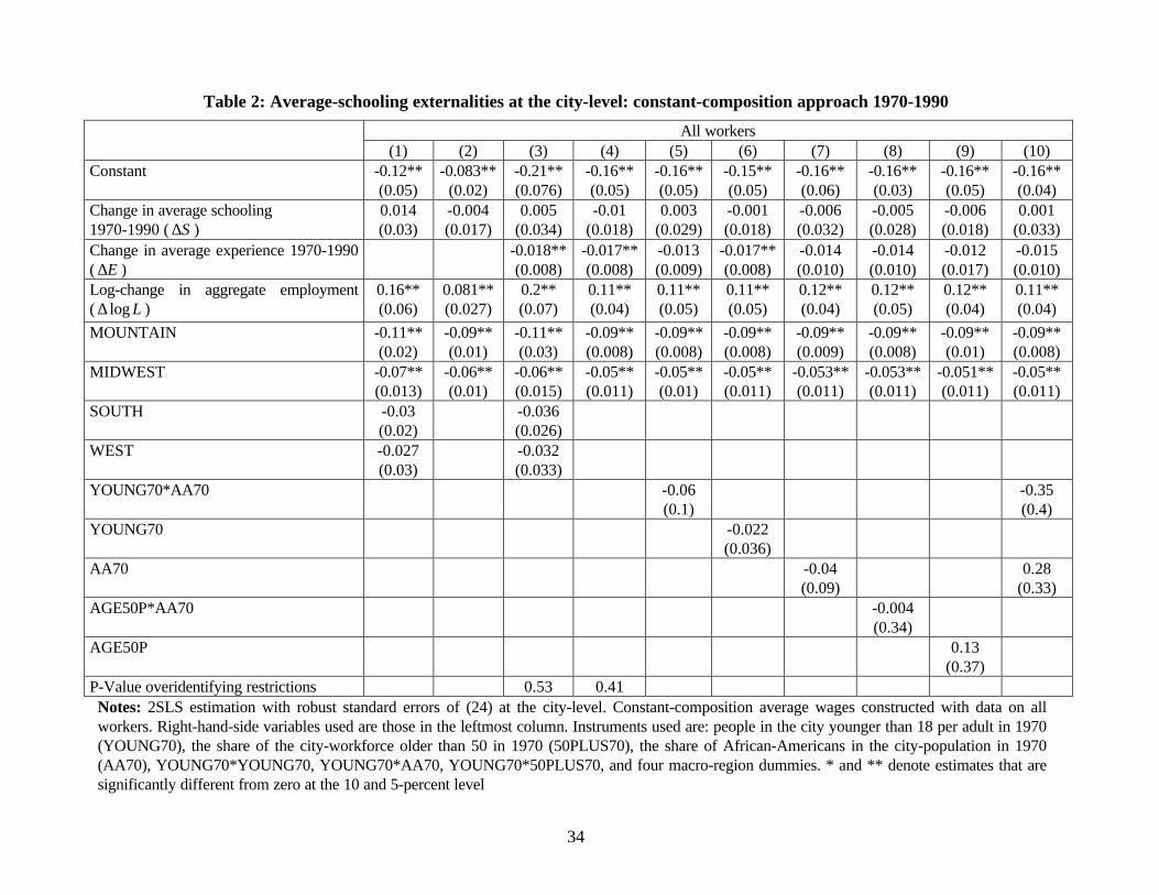
Table 2 contains the results of estimating (24) with 2SLS and the instruments discussed in
the previous section.11 Column (1) uses the constant and four (of the five) macro-region
dummies as controls. The estimate of the strength of average-schooling externalities is
0.014 with a standard error of 0.03 and hence highly insignificant. Column (2) eliminates
the (individually and jointly) insignificant macro-region dummies SOUTH and WEST. The
estimate of the strength of average-schooling externalities is now –0.004 with a standard
error of 0.017. Column (3) uses the constant and four (of the five) macro-region dummies
as well as the change in average potential experience 1970-1990 as controls. The estimate
of the strength of average-schooling externalities does not change much compared to the
specification without average experience in column (1). Changes in average potential
experience have a significantly negative effect on average wages holding workforce skill-
composition constant, which means that cities where the average age of the workforce
predicted by our instruments fell more than average saw an above-average increase of
average wages holding workforce skill-composition constant. This suggests that these cities
experienced an inflow of workers with high wages due to unobservable characteristics.12
The P-value of the test of overidentifying restrictions in the last row (0.53) indicates that
these restrictions cannot be rejected at standard significance levels. Column (4) eliminates
the (individually and jointly) insignificant macro-region dummies SOUTH and WEST. The
estimate of average-schooling externalities is now –0.01 with a standard error of 0.018. The
P-value of the test of overidentifying restrictions in the last row (0.41) indicates that these
restrictions cannot be rejected at standard significance levels. Columns (5) to (10) estimate
equation (24) using selected instruments as control variables. The direct effect of the
instruments on average wages holding workforce skill-composition constant is in all cases
small and statistically insignificant. For example, when adding the population-share of
11 Least-squares (LS) estimation of (24) is likely to yield biased estimates because both the increasein average schooling and log-employment are endogenous and measured with error. Still, in practiceLS estimates of the strength of average-schooling externalities are very similar to 2SLS estimates(the difference is at most half a percentage point) and highly insignificant. This suggests that thedifferent biases present in least-squares estimation tend to offset each other in this particularapplication.12 A piece of evidence supporting this interpretation is our finding that the partial correlation (holdingthe change in average schooling predicted by our instruments constant) between the change inaverage potential experience predicted by our instruments and the mover-stayer wage-differential isnegative.
26
African-Americans in 1970 as a control variable in column (7), we find that a 5 percentage
points increase in this share lowers average wages holding workforce skill-composition
constant by only 0.2 percent (the maximum variation in the share of African-Americans
across cities in 1970 is 25 percentage points) and that this effect is highly insignificant.
Moreover, estimates of the strength of average-schooling externalities in columns (5) to
(10) remain close to zero and insignificant.
Table 3 contains the results of estimating (24) when data on white males only is used to
construct constant-composition average wages. The method of estimation is 2SLS with the
usual instruments. Columns (1) to (5) use data on all white males adjusted for wage-
differentials related to marital status (the adjustment is based on (22)). The results are very
similar to those obtained using all workers once the (individually and jointly) insignificant
macro-region dummies SOUTH and WEST are eliminated. For example the strength of
average-schooling externalities in column (2) is –0.001 with a standard error of 0.021. The
P-value of the test of overidentifying restrictions in the last row (0.73) indicates that these
restrictions cannot be rejected at standard significance levels. Columns (6) and (7) contain
the results of estimating (24) using data on white males aged 40-49 only to construct
constant-composition average wages (these are the workers used by Acemoglu and Angrist
(2000) to estimate average-schooling externalities at the state-level). Once the (individually
and jointly) insignificant macro-region dummies SOUTH and WEST are eliminated, the
results are similar to those obtained with all white males and all workers.
Estimates of the strength of aggregate scale effects in tables 2 and 3 are very imprecise
and larger than the 4 to 10 percent effect reported in much of the literature (e.g. Henderson
(1986, 1988), Ciccone and Hall (1996)).13 To see whether our results are sensitive with
respect to the strength of aggregate scale effects we re-estimate (24) restricting aggregate
scale effects to values between 4 and 10 percent. The results are reported in table 4.
Estimates of the strength of average-schooling externalities are in all cases close to the
values obtained when the strength of aggregate scale effects is estimated.
Table 5 contains constant-composition-approach estimates of average-schooling
externalities between 1970 and 1990 at the US state-level. The method of estimation is
2SLS using either the instruments of Acemoglu and Angrist (2000) or our instruments at
the state-level. The AA instruments are based on whether state-level compulsory-schooling
(child-labor) laws when workers were 14 required 8, 9, 10, or 11 years of minimum
13 This is because our instruments predict only 22 percent of the variation of the log-change inaggregate employment 1970-1990 across cities.
27
schooling (6, 7, 8, or 9 years of schooling before work was permitted). AA construct these
instruments using both the state of residence and the state of birth of workers and find that
empirical results are very similar in the two cases. Column (1) contains the result of
average wages are constructed using data on white males aged 40-49 only, with the AA
instruments (following AA, we do not include the change in log-employment or other
control variables in the estimating equation). In particular, the instruments used are the
change between 1970 and 1990 of the fraction of workers for whom state-of-residence
compulsory-schooling (child-labor) laws when they were 14 required 8, 9, 10, or 11 years
of minimum schooling (6, 7, 8, or 9 years of schooling before work is permitted). These
instruments combined predict 45 percent of the change in average schooling 1970-1990
(not in table). Column (2) contains the result of estimating the same equation using 2SLS
with our instruments at the state-level. Our instruments predict 51 percent of the change in
average schooling 1970-1990 at the state-level (not in table). It can be seen that estimates
of the strength of average-schooling externalities obtained with both sets of instruments are
nearly identical. (The results in table 5 are not comparable to those in AA because they use
the Mincerian approach and never consider the 1970-1990 period by itself.14)
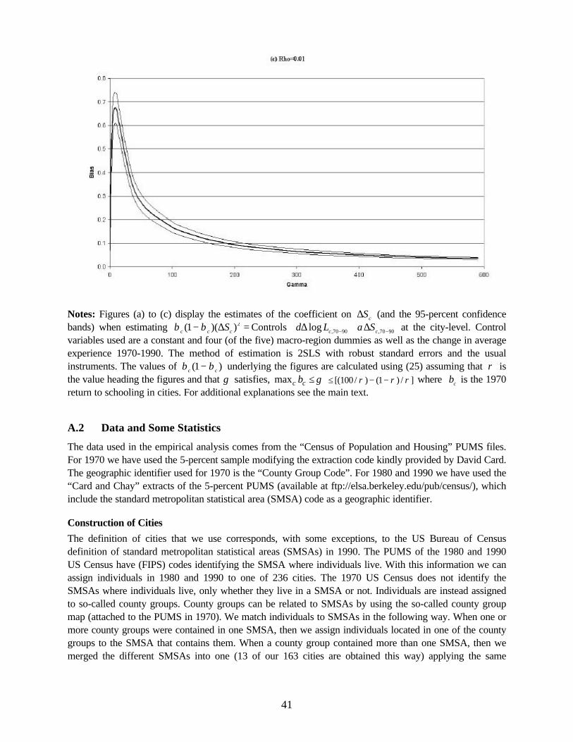
6.1.2 Second-Order Effects
Regressing 2( )cS∆ on the right-hand-side variables of (24) using 2SLS and the usual
instruments yields a coefficient on cS∆ of 2.71 with a standard error of 0.14. Figures (1a) to
(1c) deal with the sign of the bias when it cannot be assumed that the share of human capital
in the average wage is identical across cities. The figures display the estimates of the
coefficient on cS∆ (and the 95-percent confidence bands) when regressing 2ˆ ˆ(1 )( )c c cSβ β− ∆
on the right-hand-side variables of (24) using 2SLS and the usual instruments. The values ofˆ ˆ(1 )c cβ β− underlying (1a) are based on (25) assuming that 0.99ρ = and that γ satisfies
[ ]ˆ ˆmax 100/ (1 ) / minc c c cb bγ ρ ρ ρ≤ ≤ − − , where cb is the 1970 return to schooling in cities
14 To reproduce the AA results we also estimate ˆ ConstantAA
state statea Sα∆ = + ∆ for 1960-1980, where
ˆ AAstatea∆ is the 1960-1980 change in the estimated intercept of a Mincerian least-squares wage
regression at the state-level using data on white males 40-49 only. 2SLS yields an estimate of theaverage-schooling externalities equal to 0.005 with a standard error of 0.029 when using asinstruments the 1960-1980 change in the fraction of workers for whom state-of-residencecompulsory-schooling (child-labor) laws when they were 14 required 8, 9, 10, or 11 years ofminimum schooling (6, 7, 8, or 9 years of schooling before work is permitted). This estimate isalmost identical to the result of AA for the same time period.
28
estimated using (19) with a city-specific individual return to schooling. Figure (1b) and (1c)
repeat the same exercise for values of 0.5ρ = and 0.01ρ = respectively. It can be seen from
the figures that the bias is significantly positive in all three cases. Repeating the analysis for
all values of ρ between 0.01 and 0.99 in one-percent steps yields that the bias of the basic
constant-composition approach to average-schooling externalities in cities should (omitted)
second-order effects be important is significantly positive in all cases.
6.1.3 Unobserved Heterogeneity
Table 6 contains the coefficient on cS∆ when regressing the estimated city-specific mover-
stayer wage-differential cstφ on the right-hand-side variables of (24) using least squares as
well as 2SLS with the usual instruments. cstφ is estimated using (26) for the six individual
schooling intervals indicated in the table. The least-squares results indicate a significantly
positive partial correlation between the mover-stayer wage-differential and the increase in
average schooling at the city-level for workers with 9 to 17 years of schooling in 1980 and
workers with 9 to 14 years of schooling in 1990. This finding supports the view that cities
with a larger increase in average schooling attract workers with higher wages due to
unobservable characteristics. Interestingly, the results are very similar whether stayers
(“non-movers”) are defined as workers who lived in the same house since 1970 or workers
who lived in the same city five years before we observe their wages and were born in the
state where they reside. The only negative partial correlation between the mover-stayer
wage-differential and the increase in average schooling can be found for workers with 0 to 9
years of schooling and workers with 17 or more years of schooling in 1980. These estimates
are statistically insignificant however. Moreover, workers with 0 to 9 years of schooling are
a small fraction of the workforce in both 1980 (6.6 percent) and 1990 (4.3 percent).
Similarly workers with 17 or more years of schooling in 1980 are only 10 percent of the
workforce.
Table 6 also summarizes the results of regressing cstφ on the right-hand-side variables
of (24) using 2SLS with the usual instruments. It can be seen that there is no significant
relationship between the increase in average schooling and the mover-stayer wage-
differential with the exception of the significantly positive relationship for workers with 12
to 14 years of schooling in 1990. Furthermore, the estimates are all positive with the
exception of workers with 0 to 9 years of schooling in 1990. These workers are only 4.3
percent of the workforce however. The 2SLS results therefore suggest that mover-stayer
wage-differentials are not as highly correlated with the increase in average schooling
29
predicted by our instruments as with the increase in average schooling. Moreover, if our
2SLS estimates are biased because of unobserved heterogeneity and selective migration,
they are biased upwards.
6.2 The Mincerian Approach
Table 7 contains estimates of average-schooling externalities at the city-level using the
Mincerian approach in (20). The control variables, estimation method, and instruments are
the same ones used to implement the constant-composition approach. Columns (1) to (3)
contain the results when the underlying Mincerian wage regression in (19) is estimated
using all workers. According to columns (1) and (2), the external effect on productivity of
an additional year of average schooling is above 7 percent and statistically significant at the
5-percent level. Columns (1) and (2) differ in that the latter eliminates the (individually and
jointly) insignificant SOUTH and WEST macro-region dummies. Column (3) contains the
average-schooling-externality estimate when the Mincerian intercept in (19) is estimated
allowing the individual return to schooling to differ across cities. The estimate triples
compared to the two previous columns. Column (4) contains the average-schooling-
externality estimate when the Mincerian intercept is estimated using data on white males
only (restricting the individual return to schooling to be equal across cities). Results are
very similar to the case where all workers are used. The P-value of the test of
overidentifying restrictions in the last row of columns (1) to (4) indicates that these
restrictions cannot be rejected at standard significance levels.
Table 8 investigates the effect of average schooling in cities on the individual return to
schooling. All results are based on estimating (21) using 2SLS with the usual instruments.
Column (1) indicates that the change in average schooling between 1970 and 1990 does not
have a statistically significant effect on the change in the individual return to schooling when
all four macro-region dummies are included in the analysis. The four macro-region dummies
are individually and jointly insignificant at standard significance levels however (the P-value
of the joint exclusion restriction is 0.41). Columns (2) to (12) estimate the effect of the
change in average schooling 1970-1990 on the change in the individual return to schooling
when the four macro-region dummies are not used as controls. Column (2) contains the
basic specification. The results suggest that a one-year increase in average schooling
decreases the individual return to schooling by 1.5 percent (with a standard error of around
0.4 percent). The P-value of the test of overidentifying restrictions in the last row (0.83)
indicates that these restrictions cannot be rejected at standard significance levels. Columns
30
(3) to (6) include selected instruments directly into the estimating equation to see whether
they affect the results. The direct effect of the instruments on the change in individual return
to schooling is insignificant and the effect of average schooling significantly negative in all
cases. Columns (7) to (11) estimate (21) without using the four macro-region dummies as
instruments. A one-year increase in average schooling is now estimated to reduce the
individual return to schooling by around 1.1 percent (with a standard error of around 0.5
percent). Finally, column (12) estimates the effect of average schooling on the individual
return to schooling using data on white males only to estimate the individual return to
schooling. The results are very similar to the case where all workers are used.
7 Summary
When workers with different human capital are imperfect substitutes in production, an
increase in average human capital changes wages of workers with particular skills but has
no first-order effect on average wages holding workforce skill-composition constant if
wages reflect marginal social products. Based on this result, we propose an approach to
identify human capital externalities at the aggregate level that yields positive externalities if
and only if the marginal social product of workers with above-average human capital
exceeds their wage. The approach can also be used to identify human capital externalities
that are biased towards workers with high or low levels of human capital.
31
References
Acemoglu, Daron and Joshua Angrist (2000) “How Large are the Social Returns to Education:Evidence from Compulsory Schooling Laws,” in Ben S. Bernanke and Kenneth Rogoff eds,NBER Macroeconomic Annual 2000, pp 9-59.
Autor, David, Larry Katz and Alan Krueger (1998) “Computing Inequality: have Computerschanged the Labor Market?” Quarterly Journal of Economics 113 (4), pp. 1169-1213.
Azariadis, Costas and Allen Drazen (1990) “Threshold Externalities in EconomicDevelopment,” Quarterly Journal of Economics 105, pp, 501-26.
Benhabib, Jess and Mark Spiegel (1994) “The Role of Human Capital in EconomicDevelopment, Evidence from Aggregate Cross-Country Data,” Journal of MonetaryEconomics 34 (2), pp. 143-173.
Bils, Mark and Peter Klenow (2000) “Does Schooling Cause Growth?” American EconomicReview, 90, pp.1160-1193.
Black, Duncan and Vernon Henderson (1999) “A Theory of Urban Growth,” Journal ofPolitical Economy 107 (2), pp. 252-284.
Card, David and Thomas Lemieux (2000) “Can Falling Supply Explain the Rising Return toCollege for Younger Men? A Cohort Based Analysis,” NBER Working Paper No. W7655,April.
Ciccone Antonio and Robert Hall (1996) “Productivity and the Density of Economic Activity,”American Economic Review 86 (1), pp. 54-70.
Conley, Timothy, Frederick Flier, and Grace Tsiang (1999) “Local Market Human Capital andthe Spatial Distribution of Productivity in Malaysia,” Mimeo, Northwestern University,February.
De la Fuente, Angel and Raphael Domenech (2001) “Schooling Data, Technological Diffusionand the Neoclassical Model,” American Economic Review 91 (2), pp. 323-327.
Gemmell, Norman (1997) “Externalities to Higher Education,” Report to the NationalCommittee of Inquiry into Higher Education, HMSO Copyright Unit, St Clements House,Norwich.
Greene, William (1999) Econometric Analysis 4th Edition, Prentice Hall, New Jersey.Hall, Robert and Charles Jones (1999) “Why Do Some Countries Produce So Much More
Output Per Worker than Others?” Quarterly Journal of Economics, 114(1), pp. 83-116.Heckman, James and Peter Klenow (1998) “Human Capital Policy,” in Michael Boskin (editor)
Policies to Promote Capital Formation Hoover Institution.Heckman, James (2000) “Policies to Foster Human Capital,” Research in Economics 51, No 1
March, pp. 3-56.Henderson, Vernon (1986) “Efficiency of Resource Usage and City Size,” Journal of Urban
Economics 18, pp. 23-56.Henderson, Vernon (1988) Urban Development: Theory, Fact, and Illusion, Oxford
University Press, Oxford, UK.Johnson, George (1997) “Changes in Earnings Inequality: The Role of Demand Shifts,”
Journal of Economic Perspectives 11 (2), pp. 41-54.
32
Katz, Larry and Kevin Murphy (1992) “Changes in Relative Wages 1963-1987- Supply andDemand Factors,” Quarterly Journal of Economics 107 (1), pp. 35-78.
Klenow, Peter and Andres Rodriguez-Clare (1997) “The Neoclassical Revival in GrowthEconomics: Has it Gone too Far?” in Ben Bernanke and Julio Rotemberg eds. NBERMacroeconomic Annual 1997, pp.73-103, Cambridge MA. MIT Press.
Krueger, Alan and Mikael Lindahl (2001) “Education for Growth: Why and for Whom?”Journal of Economic Literature 39 (4), pp. 1101-1136.
Krugman, Paul (1992) “Increasing Returns and Economic Geography,” Journal of PoliticalEconomy 99, pp. 483-499.
Lucas, Robert E. (1988) “On the Mechanics of Economic Development,” Journal ofMonetary Economics 22, pp. 3-41.
Mankiw, Gregory, David Romer, and David Weil (1992) “A Contribution to the Empirics ofEconomic Growth” Quarterly Journal of Economics, 107 (2), pp. 407-438.
Marshall, Alfred (1890) Principles of Economics, Macmillan, London.Moomaw, Ronald (1981), “Productivity and City Size: A Critique of the Evidence,” Quarterly
Journal of Economics 95, pp. 194-223.Moretti, Enrico (2000) “Estimating the Social Return to Education: Evidence From
Longitudinal and Cross-Sectional Data,” Center for Labor Economics, University ofCalifornia, Berkeley, Working Paper No. 22.
Rauch, James (1993) “Productivity Gains from Geographic Concentration in Cities,” Journalof Urban Economics 34, pp. 380-400.
Roback, Jennifer (1982) “Wages, Rents, and the Quality of Life,” Journal of PoliticalEconomy 90, pp. 1257-1278.
Rudd, Jeremy (2000) “Empirical Evidence on Human Capital Spillovers,” Federal ReserveBoard, Finance and Economics Discussion Paper 2000-46, October.
Sveikauskas, Leo (1975), “The Productivity of Cities,” Quarterly Journal of Economics 89,pp. 393-413.
Temple, Jonathan (2001) “Growth effects of education and social capital in the OECDcountries,” OECD Economic Studies, 2001/2, 33, pp.57-101.
Topel, Robert (1997) “Factor Proportions and Relative Wages,” Journal of EconomicPerspectives, 11(2), pp. 55-74.
Topel, Robert (1999) “Labor Markets and Economic Growth,” in Handbook of LaborEconomics, ed. Orley Ashenfelter and David Card. Amsterdam: Elsevier Science, pp.2943-2984.
U.S. Bureau of Census (1970), Census of Population and Housing, United States.U.S. Bureau of Census (1980), Census of Population and Housing, United States.U.S. Bureau of Census (1990), Census of Population and Housing, United States.
US Department of Commerce (1992), Economics and Statistics Administration, Bureau of
Economic Analysis, Regional Economic Measurement Division, REIS CD-ROM.
33
Appendix
A.1 Tables and Figures
Table 1: Quality of the 1970 instruments for the change in average schooling andaverage experience 1970-1990
Change in averageschooling
1970-1990 ( S∆ )
Change in averageexperience 1970-
1990 ( E∆ )(1) (2) (3) (4)
Share of the city-workforce older than 50 in 1970(50PLUS70)
5.7**(1.1)
3.6**(1.1)
-25.3**(3.02)
-23.4**(3.34)
Share of African-Americans in the city-population in1970 (AA70)
11.6** (3.1)
6.8**(2.9)
-3.65(8.48)
1.25(8.85)
People in the city younger than 18 per adult in 1970(YOUNG70)
-3.7*(2.2)
-3.0(2.2)
12.47**(5.9)
12.79**(6.11)
YOUNG70*YOUNG70 2.7**(1.2)
2.8(2.1)
-8.1**(3.38)
-8.55**(3.44)
YOUNG70*AA70 -5.9**(2.6)
-2.9(2.5)
-6.74(7.38)
-11.18(7.47)
50PLUS70*AA70 -16.7**(8.2)
-8.8(8.2)
41.42*(24.45)
39.1*(21.23)
MIDWEST -0.17**(0.06)
-0.01(0.2)
MOUNTAIN -0.29**(0.14)
-0.14(0.42)
WEST -0.47**(0.07)
0.52**(0.23)
SOUTH -0.14**(0.07)
0.05(0.21)
2R 0.48 0.57 0.47 0.51
Notes: Results of regressing the increase in average years of schooling and average years ofpotential experience 1970-1990 at the city-level on a constant and the variables in the leftmostcolumn using least squares with robust standard errors. The number of observations is 163.YOUNG70 and YOUNG70 squared are always jointly significant at the 5-percent level. * and **denote estimates that are significantly different from zero at the 10 and 5-percent level. Thequadratic specification for YOUNG70 implies that the marginal effect of YOUNG70 on theincrease in average schooling (average experience) would be negative (positive) for small valuesof YOUNG70; for sample values the effect is always positive (negative) however.
34
Table 2: Average-schooling externalities at the city-level: constant-composition approach 1970-1990
P-Value overidentifying restrictions 0.53 0.41Notes: 2SLS estimation with robust standard errors of (24) at the city-level. Constant-composition average wages constructed with data on allworkers. Right-hand-side variables used are those in the leftmost column. Instruments used are: people in the city younger than 18 per adult in 1970(YOUNG70), the share of the city-workforce older than 50 in 1970 (50PLUS70), the share of African-Americans in the city-population in 1970(AA70), YOUNG70*YOUNG70, YOUNG70*AA70, YOUNG70*50PLUS70, and four macro-region dummies. * and ** denote estimates that aresignificantly different from zero at the 10 and 5-percent level
35
Table 3: Average-schooling externalities at the city-level: constant-composition approach 1970-1990White males White males aged
40-49(1) (2) (3) (4) (5) (6) (7)
Constant -0.25**(0.1)
-0.17**(0.07)
-0.18**(0.07)
-0.18**(0.07)
-0.17**(0.08))
-0.27**(0.11)
-0.25**(0.068)
Change in average schooling1970-1990 ( S∆ )
0.046(0.04)
-0.001(0.021)
-0.017(0.045)
-0.005(0.041)
-0.001(0.023)
0.07(0.06)
-0.015(0.03)
Change in average experience1970-1990 ( E∆ )
-0.02*(0.011)
-0.02*(0.011)
-0.02*(0.013)
-0.021*(0.013)
-0.02*(0.011)
-0.013(0.015)
-0.027**(0.012)
Log-change in aggregateemployment ( log L∆ )
0.16**(0.08)
0.13**(0.05)
0.14**(0.05)
0.14**(0.05)
0.14**(0.05)
0.16*(0.1)
0.14**(0.05)
MOUNTAIN -0.11**(0.03)
-0.12**(0.013)
-0.12**(0.012)
-0.12**(0.013)
-0.12**(0.014)
-0.035(0.059)
MIDWEST -0.029(0.019)
-0.035**(0.014)
-0.03**(0.01)
-0.035**(0.014)
-0.035**(0.014)
-0.029(0.028)
SOUTH -0.018(0.028)
-0.062(0.047)
WEST 0.026(0.052)
0.018(0.059)
YOUNG70*AA70YOUNG70 -0.005
(0.05)AA70 -0.055
(0.14)AGE50P*AA70AGE50P 0.017
(0.14)P-Value overidentifyingrestrictions
0.87 0.73 0.31 0.22
Notes: 2SLS estimation with robust standard errors of (24) at the city-level. Constant-composition average wages constructed with data on whitemales only in columns (1) to (5) and white males aged 40-49 in columns (7) and (8). Right-hand-side variables used are those in the leftmostcolumn. Instruments used are: people in the city younger than 18 per adult in 1970 (YOUNG70), the share of the city-workforce older than 50 in1970 (50PLUS70), the share of African-Americans in the city-population in 1970 (AA70), YOUNG70*YOUNG70, YOUNG70*AA70,YOUNG70*50PLUS70, and four macro-region dummies. The number of observations is 163. * and ** denote estimates that are significantlydifferent from zero at the 10 and 5-percent level.
Notes: 2SLS estimation with robust standard errors of the strength of average-schoolingexternalities at the city-level using (24) restricting the strength of aggregate scale effects δ to thevalues in the leftmost column. Instruments used are: people in the city younger than 18 per adult in1970 (YOUNG70), the share of the city-workforce older than 50 in 1970 (50PLUS70), the shareof African-Americans in the city-population in 1970 (AA70), YOUNG70*YOUNG70,YOUNG70*AA70, YOUNG70*50PLUS70, and four macro-region dummies. The number ofobservations is 163. * and ** denote estimates that are significantly different from zero atthe 10 and 5-percent level. The control variables used are:
• Column (1): a constant and four macro-region dummies. The P-value of the hypothesis that themacro-region dummies SOUTH and WEST can be excluded from the estimating equation is0.43.
• Column (2): same as in (1) plus the increase in average experience. The P-value of thehypothesis that the macro-region dummies SOUTH and WEST can be excluded from theestimating equation is 0.57.
• Column (3): a constant and two macro-region dummies (MOUNTAIN, MIDWEST) plusincrease in average experience. The P-values of the test of overidentifying restrictions (not inthe table) indicate that these restrictions cannot be rejected at standard significance levels forthe values of δ in the table.
Table 5: Average-schooling externalities at the state-level: constant-compositionapproach 1970-1990
White males aged 40-49Change in average schooling at the US state-level1970-1990 ( S∆ )
Notes: 2SLS estimation at the US state-level of sˆlog ConstantFsw Sα∆ = + ∆ for 1970-1990,
where state-level constant-composition average wages are constructed using white males aged40-49 only. AAIV refers to the instruments used by Acemoglu and Angrist (2000) andOURIV refers to our instruments used at the state-level. The number of observations is 49.See the main text for additional explanations.
37
Table 6: Effect of change in average schooling 1970-1990 on mover-stayer wage-differential ( cstφ )
Years of schooling of workers ( s )
[ )0,9 [ )9,12 [ )12,14 [ )14,16 [ )16,17 [ )17 and more
Sample A, 1980, least squares (LS) -0.024(0.058)
0.034*(0.022)
0.037*(0.015)
0.092*(0.026)
0.038**(0.019)
-0.014(0.031)
Sample A, 1980, 2SLS 0.13(0.15)
0.023(0.035)
0.005(0.024)
0.075(0.04)
0.037(0.028)
0.09(0.13)
Sample B, 1980, LS -0.04(0.064)
0.038*(0.024)
0.04**(0.016)
0.09**(0.03)
0.035(0.021)
-0.027(0.038)
Sample B, 1980, 2SLS 0.11(0.1)
0.027(0.038)
0.01(0.026)
0.068(0.046)
0.04(0.032)
0.045(0.15)
Sample A, 1990, LS -0.12(0.09)
0.057*(0.036)
0.057**(0.018)
0.014(0.029)
0.016(0.03)
0.012(0.037)
Sample A, 1990, 2SLS -0.16(0.13)
0.028(0.056)
0.062**(0.029)
0.036(0.026)
0.047(0.047)
0.032(0.07)
Sample B, 1990, LS -0.12(0.1)
0.077*(0.043)
0.066**(0.021)
0.025(0.036)
0.063(0.051)
0.1*(0.056)
Sample B, 1990, 2SLS -0.13(0.13)
0.098(0.068)
0.062*(0.033)
0.056(0.056)
0.048(0.063)
0.1(0.08)
Notes: 2SLS estimation with robust standard errors of the effect of the change in average schooling 1970-1990 on the mover-stayerwage-differentials cstφ , 1980,1990t = , at the city-level using ,70 90 ,70 90
ˆ Controls logcst c cL Sφ δ α− −= + ∆ + ∆ . The mover-stayer wage-differentials cstφ are estimated using (26) for the six individual schooling intervals heading the table. Control variables used are aconstant and four (of the five) macro-region dummies as well as the change in average experience 1970-1990. Sample A refers to allworkers who did not live in the city five years before we observe their wages (“movers”) plus workers who lived in the same housesince 1970. Sample B refers all workers who did not live in the city five years before we observe their wages (“movers”) plus workerswho already lived in the same city five years before and were born in the state of residence. Instruments used for 2SLS estimation are:people in the city younger than 18 per adult in 1970 (YOUNG70), the share of the city-workforce older than 50 in 1970 (50PLUS70),the share of African-Americans in the city-population in 1970 (AA70), YOUNG70*YOUNG70, YOUNG70*AA70,YOUNG70*50PLUS70, and four macro-region dummies. The number of observations is 163. * and ** denote estimates that aresignificantly different from zero at the 10 and 5-percent level.
Change in average experience 1970-1990 ( E∆ ) -0.017*(0.01)
-0.013*(0.008)
-0.012(0.025)
-0.016*(0.01)
Log-change in aggregate employment ( log L∆ ) 0.28**(0.08)
0.16**(0.04)
0.36**(0.13)
0.22**(0.09)
MOUNTAIN -0.09**(0.026)
-0.053**(0.013)
-0.084**(0.041)
-0.16**(0.03)
MIDWEST 0.066**(0.016)
-0.055**(0.012)
-0.069**(0.034)
-0.054**(0.017)
SOUTH -0.047(0.035)
WEST -0.047(0.036)
P-Value overidentifying restrictions 0.64 0.21 0.27 0.23Individual return assumed identical across cities? Yes Yes No Yes
Notes: 2SLS estimation with robust standard errors of (20) at the city-level. Mincerian intercepts are estimated with data on all workers incolumns (1) to (3) and white males only in column (4). Right-hand-side variables used are those in the leftmost column. Instruments used are:people in the city younger than 18 per adult in 1970 (YOUNG70), the share of the city-workforce older than 50 in 1970 (50PLUS70), the shareof African-Americans in the city-population in 1970 (AA70), YOUNG70*YOUNG70, YOUNG70*AA70, YOUNG70*50PLUS70, and fourmacro-region dummies. The number of observations is 163. * and ** denote estimates that are significantly different from zero at the 10 and 5-percent level.
39
Table 8: Effect of average schooling on the individual return to schooling 1970-1990
Macro-region controls? Yes No No No No No No No No No No NoYOUNG70*AA70 0.006
(0.03)YOUNG70 -0.002
(0.008)-0.01
(0.011)AA70 0.027
(0.026)-0.007(0.02)
AGE50P*AA70AGE50P 0.12
(0.09)-0.021(0.06)
P-Value overidentifyingrestrictions
0.74 0.83 0.61 0.81 0.75
Comments Macro-region dummies not used as instruments
Notes: 2SLS estimation with robust standard errors of (21) at the city-level. Individual returns to schooling are estimated with data on all workers incolumns (1) to (11) and white males only in column (12). Right-hand-side variables used are those in the leftmost column. Instruments used are: peoplein the city younger than 18 per adult in 1970 (YOUNG70), the share of the city-workforce older than 50 in 1970 (50PLUS70), the share of African-Americans in the city-population in 1970 (AA70), YOUNG70*YOUNG70, YOUNG70*AA70, YOUNG70*50PLUS70, and four macro-regiondummies. The number of observations is 163.* and ** denote estimates that are significantly different from zero at the 10 and 5-percent level.
40
Figure 1: Signing the bias if second-order effects are important
41
Notes: Figures (a) to (c) display the estimates of the coefficient on cS∆ (and the 95-percent confidencebands) when estimating 2
,70 90 ,70 90ˆ ˆ(1 )( ) Controls logc c c c cS L Sβ β δ α− −− ∆ = + ∆ + ∆ at the city-level. Control
variables used are a constant and four (of the five) macro-region dummies as well as the change in averageexperience 1970-1990. The method of estimation is 2SLS with robust standard errors and the usualinstruments. The values of ˆ ˆ(1 )c cβ β− underlying the figures are calculated using (25) assuming that ρ isthe value heading the figures and that γ satisfies, ˆmaxc cb γ≤ [(100/ ) (1 ) / ]ρ ρ ρ≤ − − where cb is the 1970return to schooling in cities. For additional explanations see the main text.
A.2 Data and Some Statistics
The data used in the empirical analysis comes from the “Census of Population and Housing” PUMS files.For 1970 we have used the 5-percent sample modifying the extraction code kindly provided by David Card.The geographic identifier used for 1970 is the “County Group Code”. For 1980 and 1990 we have used the“Card and Chay” extracts of the 5-percent PUMS (available at ftp://elsa.berkeley.edu/pub/census/), whichinclude the standard metropolitan statistical area (SMSA) code as a geographic identifier.
Construction of Cities
The definition of cities that we use corresponds, with some exceptions, to the US Bureau of Censusdefinition of standard metropolitan statistical areas (SMSAs) in 1990. The PUMS of the 1980 and 1990US Census have (FIPS) codes identifying the SMSA where individuals live. With this information we canassign individuals in 1980 and 1990 to one of 236 cities. The 1970 US Census does not identify theSMSAs where individuals live, only whether they live in a SMSA or not. Individuals are instead assignedto so-called county groups. County groups can be related to SMSAs by using the so-called county groupmap (attached to the PUMS in 1970). We match individuals to SMSAs in the following way. When one ormore county groups were contained in one SMSA, then we assign individuals located in one of the countygroups to the SMSA that contains them. When a county group contained more than one SMSA, then wemerged the different SMSAs into one (13 of our 163 cities are obtained this way) applying the same
42
criterion to SMSAs in 1980 and 1990 (to ensure that cities are defined in the same way in 1970, 1980, and1990). Finally, when a county group was contained partly in a SMSA and partly in a non-SMSA area, thenwe assigned all individuals located in the county group who lived in a SMSA to the SMSA that containedpart of the county group. This procedure resulted in 163 cities for 1970, 1980, and 1990. The code toperform the identification and merge of cities is available from us upon request.
Definition of Individual Wages and Schooling
Hourly wages in a given year have been calculated as yearly salary and wage divided by weeks workedtimes average hours per week worked in the year. All regressions are run using only individuals withpositive hours worked and non-negative potential experience. All variables refer to the year previous to thecensus. Top-codes differ across years. Individual years of schooling have been obtained in the followingway. For 1970 and 1980, we use the variables “Highest Grade Attended” and “Grade” which yieldsnineteen levels of schooling. For 1990, we use the variable “Yearsch” which yields eleven levels ofschooling. When we only observe an interval for years of schooling, we use the midpoint of the interval asyears of schooling in the Mincerian wage regressions in (19). Years of experience used in (19) is potentialexperience, i.e. age minus years of schooling minus six. For the constant-composition approach in (23) wepartition years of schooling in seven intervals [0-4), [4-9), [9-12), [12-14), [14-16), [16-17), and [17 andmore) and years of experience in five intervals [0-10), [10-20), [20-30), [30-40), [40-more).
Wages and Workforce Composition by Schooling
Sample values for average hourly wages in 1990 US$ and workforce shares for the 7 education groups (atthe national level) are given in the next table.