Identifying Information Asymmetry in Securities Markets ✩ Kerry Back Jones Graduate School of Business and Department of Economics Rice University, Houston, TX 77005, U.S.A. Kevin Crotty Jones Graduate School of Business Rice University, Houston, TX 77005, U.S.A. Tao Li Department of Economics and Finance City University of Hong Kong, Kowloon, Hong Kong Abstract We propose and estimate a model of endogenous informed trading that is a hybrid of the PIN and Kyle models. When an informed trader trades optimally, both returns and order flows are needed to identify information asymmetry parameters. Empirical relationships between parameter estimates and price impacts and between parameter estimates and stochastic volatility are consistent with theory. We illustrate how the estimates can be used to detect information events in the time series and to characterize the information content of prices in the cross section. We also compare the estimates to those from other models on various criteria. ✩ Versions of this paper were presented under various titles at the University of Colorado, the SEC, the AFA Conference, the NYU Stern Microstructure Conference, the University of Chicago Market Microstructure and High Frequency Data Conference, the ASU Sonoran Winter Finance Conference, the UBC Winter Finance Conference, and the ITAM Finance Conference. We thank Pete Kyle, Rob Engle, Dmitry Livdan, Yajun Wang, and seminar participants for helpful comments, and we thank Slava Fos for helpful comments and for sharing his data on trading by Schedule 13D filers. Email addresses: [email protected](Kerry Back), [email protected](Kevin Crotty), [email protected](Tao Li) August 31, 2017
Transcript
Identifying Information Asymmetry in Securities MarketsI
Kerry Back
Jones Graduate School of Business and Department of Economics
Rice University, Houston, TX 77005, U.S.A.
Kevin Crotty
Jones Graduate School of Business
Rice University, Houston, TX 77005, U.S.A.
Tao Li
Department of Economics and FinanceCity University of Hong Kong, Kowloon, Hong Kong
Abstract
We propose and estimate a model of endogenous informed trading that is a hybrid of the PIN
and Kyle models. When an informed trader trades optimally, both returns and order flows
are needed to identify information asymmetry parameters. Empirical relationships between
parameter estimates and price impacts and between parameter estimates and stochastic
volatility are consistent with theory. We illustrate how the estimates can be used to detect
information events in the time series and to characterize the information content of prices
in the cross section. We also compare the estimates to those from other models on various
criteria.
IVersions of this paper were presented under various titles at the University of Colorado, the SEC, the AFAConference, the NYU Stern Microstructure Conference, the University of Chicago Market Microstructure andHigh Frequency Data Conference, the ASU Sonoran Winter Finance Conference, the UBC Winter FinanceConference, and the ITAM Finance Conference. We thank Pete Kyle, Rob Engle, Dmitry Livdan, YajunWang, and seminar participants for helpful comments, and we thank Slava Fos for helpful comments and forsharing his data on trading by Schedule 13D filers.
Information asymmetry is a fundamental concept in economics, but its estimation is chal-
lenging because private information is generally unobservable. Many proxies for information
asymmetry exist including bid/ask spreads, price impacts, and estimates from structural
models. In this paper, we study the identification of information asymmetry parameters
in structural models. Structural modeling allows the econometrician to capture parameters
related to the underlying economic mechanisms such as the probability and magnitude of pri-
vate information events or the intensity of liquidity trading. Demand for plausible measures
of information asymmetry is high because private information plays a key role in so many
economic settings. Evidence of this demand is the large literature in finance and accounting
that utilizes the probability of informed trade (PIN) measure of Easley, Kiefer, O’Hara and
Paperman (1996) to proxy for information asymmetry.1
Our first contribution is to propose and solve a model of informed trading in securities
markets that shares many features of the PIN model of Easley et al. (1996) but in which
informed trading is endogenous as in Kyle (1985). We call this a hybrid PIN-Kyle model.
In the paper, we study a binary signal following Easley et al. (1996), but the model can
accommodate more general signal distributions.
An important implication of the model is that order flows alone cannot identify informa-
tion asymmetry. The intuition is quite simple. Consider, for example, a stock for which there
is a large amount of private information and another for which there is only a small amount
of private information. If it is anticipated that private information is more of a concern for
the first stock than for the second, then the first stock will be less liquid, other things being
equal. The lower liquidity will reduce the amount of informed trading, possibly offsetting the
1Some of those papers assesses whether information risk is priced. See, for example, Easley and O’Hara(2004), Duarte and Young (2009), Mohanram and Rajgopal (2009), Easley, Hvidkjaer and O’Hara (2002),Easley, Hvidkjaer and O’Hara (2010), Akins, Ng and Verdi (2012), Li, Wang, Wu and He (2009), and Hwang,Lee, Lim and Park (2013). Many other papers use PIN (and other measures) to capture a firm’s informationenvironment in a variety of applications ranging from corporate finance (e.g., Chen, Goldstein and Jiang,2007; Ferreira and Laux, 2007) to accounting (e.g., Frankel and Li, 2004; Jayaraman, 2008).
1
increase in informed trading due to greater private information. In equilibrium, the amount
of informed trading may be the same in both stocks, despite the difference in information
asymmetry. In general, the distribution of order flows need not reflect the degree of infor-
mation asymmetry when liquidity providers react to information asymmetry and informed
traders react to liquidity. Thus, we provide the first theoretical explanation of why method-
ologies that use order flows alone to estimate information asymmetry parameters, like PIN
and Adjusted PIN (Duarte and Young, 2009), may not identify private information.2
Our second contribution is to develop novel estimates characterizing the information
environment in financial markets. We structurally estimate our theoretical model for a
panel of stocks and provide several validation checks that the estimated parameters are
plausibly related to information asymmetry. First, reduced-form estimates of price impact
are increasing in our structural estimates of the probability and magnitude of information
events, as implied by theory. Second, the model implies that the magnitude of price changes
is proportional to Kyle’s lambda, which depends on order flows and parameters of the model.
Empirically, volatility over the latter part of a trading day is increasing in the conditional
model-implied lambda, where the conditioning is based on cumulative order flows over the
first part of the day and our estimated parameters. This phenomenon of stochastic volatility
occurs in both the model and the data.3
2Several papers argue that PIN does not identify private information. Aktas et al. (2007) examinetrading around merger announcements. They show that PIN decreases prior to announcements. In contrast,percentage spreads and the permanent price impact of trades, measured as in Hasbrouck (1991), rise beforeannouncements, indicating the presence of information asymmetry. They describe the decline in PIN priorto announcements as a PIN anomaly. Akay et al. (2012) show that PIN is higher in the Treasury bill marketthan it is in markets for individual stocks. Given that it is very doubtful that informed trading in T-bills isa frequent occurrence, this is additional evidence that PIN is not measuring information asymmetry. Benosand Jochec (2007) find that PIN is higher following earnings announcements, contrary to their assumptionthat information asymmetry should be higher before announcements. Duarte, Hu and Young (2016) alsoexamine earnings announcements. They estimate the parameters of the PIN model and then compute theconditional probability of an information event each day. They show that the conditional probability risesprior to announcements but stays elevated for a number of days following announcements. They show thatthe high post-announcement conditional probabilities are due to high turnover and argue that high turnoveris misidentified as private information by the PIN model.
3Banerjee and Green (2015) solve a rational expectations model with myopic mean-variance investorsin which investors learn whether other investors are informed. They show that variation over time in theperceived likelihood of informed trading induces volatility clustering. While their model is quite different
2
To demonstrate potential applications of the estimates, we revisit two settings in which
PIN estimates have been employed. One application of PIN has been to attempt to capture
time-series variation in information asymmetry.4 We show that conditional probabilities of
information events calculated using order flows and our parameter estimates rise on average
around earnings announcements and are higher both pre- and post-announcement for an-
nouncements with larger absolute earnings surprises. Private information is more likely to
be present around such announcements. Conditional probabilities are also elevated during
block accumulations by Schedule 13D filers, which existing information asymmetry measures
fail to detect (Collin-Dufresne and Fos, 2015). These results indicate that the model does
capture time-series variation in information asymmetry.
The second application illustrates how estimates of the information asymmetry parame-
ters from our model can be used to augment studies concerned with cross-sectional differences
in the information content of prices. To do so, we consider the hypothesis of Chen, Goldstein
and Jiang (2007) that corporate investment is more sensitive to market prices when there is
more private information in prices. Our model allows us to measure the amount of private
information alternatively by the frequency of private information events, by the magnitude
of private information, and by the fraction of total price movement that is due to private
information. We show that corporate investment is more sensitive to prices when any of
these measures is higher. These measures of private information should prove useful in other
settings in which researchers are interested in capturing distinct facets of the information
environment (e.g., the amount of liquidity trading or the magnitude of private information).
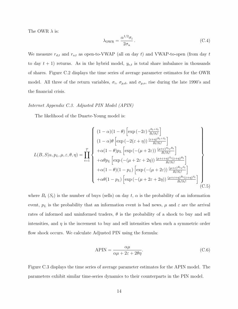
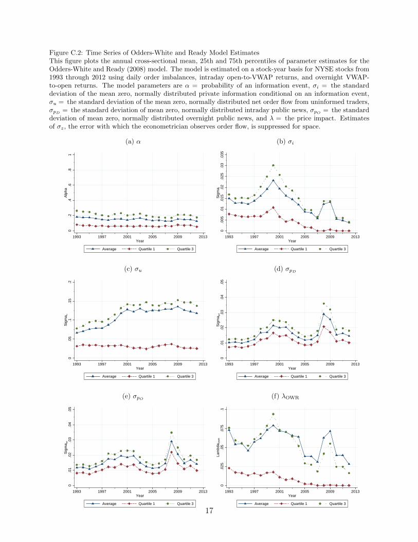
Related structural models of informed trading include the Adjusted PIN (APIN) model of
Duarte and Young (2009), the Volume-Synchronized PIN (VPIN) model of Easley, Lopez de
Prado and O’Hara (2012), and the modified Kyle model of Odders-White and Ready (2008).
from ours, our model also exhibits volatility clustering. Volatility follows the same pattern as Kyle’s lambda,which varies over time due to variation in the market’s estimate of whether an information event occurred.
4For example, Brown, Hillegeist and Lo (2004, 2009) examine changes in information asymmetry followingvoluntary conference calls and earnings surprises, respectively, while Duarte, Han, Harford and Young (2008)study the effect of Regulation FD on PIN and the cost of capital.
3
The APIN model allows for time variation in liquidity trading (with positively correlated
buy and sell intensities), which provides a better fit to the empirical distribution of buys and
sells. The VPIN model estimates buys and sells within a given time interval by assigning a
fraction of total volume to buys and the remaining fraction to sells based on standardized
price changes during the time interval.5 Odders-White and Ready (OWR) analyze a Kyle
model in which the probability of an information event is less than 1, as it is in our model.
However, they analyze a single-period model, whereas we study a dynamic model. Unlike
our dynamic model in which prices equal conditional expectations, market makers in their
model only match unconditional means of prices to unconditional means of asset values.6
Our estimate of the probability of an information event is not positively correlated in the
cross section with estimates from the other models. The divergence between the estimates is
not surprising, because the models have different assumptions/implications regarding what
data is required to identify the probability of an information event.7 We also calculate a
composite measure of information asymmetry in our model: the expected average lambda.
This measure incorporates both the probability and magnitude of information events as
well as the amount of liquidity trading. Unlike the probability of an information event, the
expected average lambda from our model is positively correlated with similar measures from
other models (PIN, APIN, VPIN, and the OWR lambda). Each of these measures should
be increasing in the probability of an information event, so it is surprising that they are all
positively correlated, given the lack of correlation of the ‘probability of an information event’
5Easley et al. (2011) claim that VPIN predicted the “flash crash” of May 6, 2010. This claim and someother claims regarding VPIN are challenged by Andersen and Bondarenko (2014b). See also Easley et al.(2014) and Andersen and Bondarenko (2014a).
6In a single-period model, because of the net order having a mixture distribution, the conditional expec-tation of the asset value given the net order is not a linear function of the net order. We solve our model byexploiting the local linearity of continuous time. Odders-White and Ready instead deviate from the usualKyle model hypothesis that prices equal conditional expected values and instead find a linear pricing rule forwhich unconditional expected market maker profits are zero. Such a pricing rule would require commitmentby market makers, because it is not consistent with ex-post optimization by market makers.
7While the OWR model uses both prices and order flows for estimation, their model shares the featureof the PIN model that the unconditional order flow distribution depends on the information asymmetryparameters and hence could be used to identify information asymmetry.
4
estimates. However, the measures are also decreasing in the amount of liquidity trading, and
we present evidence in Section 5 that the measurement of liquidity trading is quite positively
correlated across models, resulting in the positive correlation of the composite measures. Of
course, applications of the measures generally assume that they are correlated with private
information, not just inversely correlated with liquidity trading.
Theory predicts that orders have larger price impacts and quoted spreads when infor-
mation asymmetry is more severe.8 Note that this is true in both the Kyle (1985) model
upon which the hybrid and OWR models are based and the Glosten and Milgrom (1985)
model upon which PIN models are based. To test this implication of theory, we compute
reduced-form estimates of price impacts for our sample as well as quoted spreads. Empir-
ically, expected average lambda from the hybrid model is positively correlated with price
impacts and quoted spreads both in the time series and cross-sectionally. While the same
is also true for PIN, APIN, VPIN, and the OWR lambda, expected average lambda has a
higher correlation with price impacts and spreads in the time series than the other compos-
ite measures. Expected average lambda also adds explanatory power relative to the other
measures in cross-sectional regressions of price impacts or quoted spreads on the composite
measures.
Other related theoretical work includes Rossi and Tinn (2010), Foster and Viswanathan
(1995), Chakraborty and Yilmaz (2004), Goldstein and Guembel (2008), Banerjee and Breon-
Drish (2017), and Wang and Yang (2017). Rossi and Tinn solve a two-period Kyle model
in which there are two large traders, one of whom is certainly informed and one of whom
may or may not be informed. In their model, unlike ours, there are always information
events. Foster and Viswanathan (1995) consider a series of single-period Kyle models in
which traders choose in each period whether to pay a fee to become informed. There may
8There seems to be general agreement that at least a portion of the price impact of trades is due toinformation asymmetry. Glosten and Harris (1988), Hasbrouck (1988), and Hasbrouck (1991) estimatemodels of trades and price changes in which both information asymmetry and inventory control motives areaccommodated, and all three papers conclude that information asymmetry is important.
5
be periods in which there are no informed traders. However, in their model, it is always
common knowledge how many traders choose to become informed, so, in contrast to our
model, there is no learning from orders about whether informed traders are present.
Chakraborty and Yilmaz (2004) and Goldstein and Guembel (2008) study discrete-time
Kyle models in which there may or may not be an information event. The main result
in Chakraborty and Yilmaz (2004) is that the informed trader will manipulate (sometimes
buying when she has bad information and/or selling when she has good information) if the
horizon is sufficiently long. The primary difference between their model and ours is that
they assume that the liquidity trade distribution has finite support, so market makers may
incorrectly rule out a type of trader if the horizon is sufficiently long. In contrast, market
makers in our model can never rule out any type of the informed trader until the end of
the model, so it does not strictly pay for a low type to pretend to be a high type or vice
versa. The primary focus of Goldstein and Guembel (2008) concerns the incentives for an
uninformed strategic trader to manipulate if information in financial markets feeds back
into managers’ investment decisions. In their benchmark equilibrium with no feedback, the
uninformed speculator behaves as a contrarian but does not manipulate, which is the case
in our equilibrium.
Banerjee and Breon-Drish (2017) and Wang and Yang (2017) study continuous-time
Kyle models (specifically, the model of Back and Baruch (2004) in which there is a random
announcement date) in which an informed trader may not be present. Banerjee and Breon-
Drish study the information acquisition decision, treating it as a real option. In one version
of their model, the timing of information acquisition is publicly observed. In that version,
the market is infinitely deep before information is acquired, and the model is essentially
the same as in Back and Baruch after information is acquired. In a second version of their
model, the timing of information acquisition is not publicly observed, and the market tries
to learn from orders whether information has been acquired. For that version, they establish
a nonexistence result: In the class of pricing rules they consider, there is no equilibrium.
6
Wang and Yang also study the Back-Baruch version of the Kyle model. In their model,
nature chooses at date 0 whether there is an information event (and all information events
are “good news” events). Unlike in our model or the model of Banerjee and Breon-Drish,
the strategic trader is not present in their model when there is no information event.9 They
also show the nonexistence of equilibria (though they have an existence result for a second
version of their model in which the market maker is a monopolist).
2. The Hybrid Model
The hybrid model includes two important features of PIN models—a probability less
than 1 of an information event and a binary asset value conditional on an information
event—and it also includes an optimizing (possibly) informed trader, as in the Kyle (1985)
model. Denote the time horizon for trading by [0, 1]. Assume there is a single risk-neutral
strategic trader. Assume this trader receives a signal S ∈ L,H at time 0 with probability
α, where L < 0 < H.10 Let pL and pH = 1 − pL denote the probabilities of low and high
signals, respectively, conditional on an information event. With probability 1−α, there is no
information event, and the trader also knows when this happens. Let ξ denote an indicator
for whether an information event has occurred (ξ = 1 if yes and ξ = 0 if no). In addition
to the private information, public information can also arrive during the course of trading,
represented by a martingale V . Whether there was an information event, and, if so, whether
the signal was low or high becomes public information after the close of trading at date 1,
producing an asset value of V1 + ξS. Without loss of generality, we take the signal S to
have a zero mean. We can always do this by taking the signal mean to be part of the public
information V0.
In addition to the strategic trades, there are liquidity trades represented by a Brownian
motion Z with zero drift and instantaneous standard deviation σ. Let Xt denote the number
9We call the strategic trader when there is no information event a “contrarian trader.” See Section 2.2for discussion.
10Internet Appendix A extends the model to general signal distributions.
7
of shares held by the strategic trader at date t (taking X0 = 0 without loss of generality),
and set Yt = Xt + Zt. The processes Y and V are observed by market makers. Denote the
information of market makers at date t by FV,Yt .
One requirement for equilibrium in this model is that the price equal the expected value
of the asset conditional on the market makers’ information and given the trading strategy
of the strategic trader:
Pt = E[V1 + ξS | FV,Yt
]= Vt + E
[ξS | FV,Yt
]. (1)
We will show that there is an equilibrium in which Pt = Vt + p(t, Yt) for a function p. This
means that the expected value of ξS conditional on market makers’ information depends
only on cumulative orders Yt and not on the entire history of orders.
The other requirement for equilibrium is that the strategic trades are optimal. Let θt
denote the trading rate of the strategic trader (i.e., dXt = θt dt). The process θ has to
be adapted to the information possessed by the strategic trader, which is V , ξS, and the
history of Z (in equilibrium, the price reveals Z to the informed trader). The strategic trader
chooses the rate to maximize
E
∫ 1
0
[V1 + ξS − Pt] θt dt = E
∫ 1
0
[ξS − p(t, Yt)] θt dt , (2)
with the function p being regarded by the informed trader as exogenous. In the optimization,
we assume that the strategic trader is constrained to satisfy the “no doubling strategies”
condition introduced in Back (1992), meaning that the strategy must be such that
E
∫ 1
0
p(t, Yt)2 dt <∞
with probability 1.
Let N denote the standard normal distribution function, and let n denote the standard
8
normal density function. Set yL = σN−1(αpL) and yH = σN−1(1− αpH). This means that
the probability mass in the lower tail (−∞, yL) of the distribution of cumulative liquidity
trades Z1 equals αpL, which is the unconditional probability of bad news. Likewise, the
probability mass in the upper tail (yH ,∞) of the distribution of Z1 equals αpH , which is the
unconditional probability of good news. Set
q(t, y, s) =
E[Z1 − Zt | Zt = y, Z1 < yL] if s = L ,
E[Z1 − Zt | Zt = y, yL ≤ Z1 ≤ yH ] if s = 0 ,
E[Z1 − Zt | Zt = y, Z1 > yH ] if s = H .
(3)
From the standard formula for the mean of a truncated normal, we obtain the following more
explicit formula for q:
q(t, y, s)
σ√
1− t =
− n
(yL−yσ√
1−t
)/N(yL−yσ√
1−t
)if s = L ,[
n(yL−yσ√
1−t
)− n
(yH−yσ√
1−t
)]/[N(yH−yσ√
1−t
)− N
(yL−yσ√
1−t
)]if s = 0 ,
n(y−yHσ√
1−t
)/N(y−yHσ√
1−t
)if s = H .
(4)
The equilibrium described in Theorem 1 below can be shown to be the unique equilibrium in a
certain broad class, following Back (1992). The proof of Theorem 1 is given in Appendix A.11
Theorem 1. There is an equilibrium in which the trading rate of the strategic trader is
θt =q(t, Yt, ξS)
1− t . (5)
Given market makers’ information at any date t, the conditional probability of an information
11The proof is based on a generalization of the Brownian bridge feature of the continuous-time Kyle modelestablished in Back (1992). Whereas a Brownian bridge is a Brownian motion conditioned to end at aparticular point, in this model (with a discrete rather than continuous distribution of the asset value) weencounter a Brownian motion conditioned only to end in a particular interval. The generalization of theBrownian bridge is established as a lemma in Appendix A.
9
event with a low signal is N(yL−Ytσ√
1−t
)and the conditional probability of an information event
with a high signal is N(Yt−yHσ√
1−t
). The equilibrium asset price is Pt = Vt + p(t, Yt), where the
pricing function p is given by
p(t, y) = L · N(yL − yσ√
1− t
)+H · N
(y − yHσ√
1− t
). (6)
In this equilibrium, the process Y is a martingale given market makers’ information and
has the same unconditional distribution as does the liquidity trade process Z; that is, it is a
Brownian motion with zero drift and standard deviation σ.
The last statement of the theorem implies that the distribution of order flows in the
model does not depend on the information asymmetry parameters α, H, and L. Thus, if
the model is correct, it is impossible to estimate those parameters using order flows alone.
In general, the theorem suggests that it may be difficult to identify information asymmetry
parameters using order flows alone, as discussed in the introduction and the next subsection.
When we estimate the hybrid model, we use both order flows and returns, in contrast to
related models that only use order flows.
Empirically, we test the relationship between α and price impacts of trades. Figure 1
plots the equilibrium price as a function of Yt for two different values of α. It shows that the
price is more sensitive to orders when α is larger. To investigate further how the sensitivity
of prices to orders depends on α in the hybrid model, we calculate the price sensitivity—that
is, we calculate Kyle’s lambda.
Theorem 2. In the equilibrium of Theorem 1, the asset price evolves as dPt = dVt +
λ(t, Yt) dYt, where Kyle’s lambda is
λ(t, y) = − L
σ√
1− t · n(yL − yσ√
1− t
)+
H
σ√
1− t · n(yH − yσ√
1− t
). (7)
Furthermore, Kyle’s lambda λ(t, Yt) is a martingale with respect to market makers’ informa-
10
tion on the time interval [0, 1).
Kyle’s lambda is a stochastic process in our model, but we can easily relate the expected
average lambda to α. Because lambda is a martingale, the expected average lambda is
λ(0, 0). Substitute the definitions of yL and yH in (7) to compute12
λ(0, 0) = −Lσ
n(N−1(αpL)
)+H
σn(N−1(1− αpH)
). (8)
Figure 2 plots the expected average lambda as a function of α for two values of H, taking
L = −H. Doubling the signal magnitudes doubles lambda. Furthermore, the expected
average lambda is increasing in α.
2.1. Nonidentifiability Using Order Flows Alone
A key result of Theorem 1 is that the aggregate order imbalance Y1 has the same distri-
bution as the liquidity trades Z1 and is invariant with respect to the information asymmetry
parameters.13 Further insight into this identification issue can be gained by noting that the
unconditional distribution of the order imbalance in our model is a mixture of three con-
ditional distributions. With probability αpL, Y1 is drawn from the distribution conditional
on a low signal; with probability αpH , Y1 is drawn from the distribution conditional on a
high signal; and with probability 1 − α, Y1 is drawn from the distribution conditional on
no information event. The first two distributions have nonzero means—there is an excess
of sells over buys in the first and an excess of buys over sells in the second. One might
conjecture that changing α—thereby changing the likelihood of drawing from the first two
distributions—will alter the unconditional distribution of Y1. If so, then one could perhaps
12If information events occur for sure (α = 1), then λ(0, 0) = (H − L) n(0)/σ. This is analogous to theresult of Kyle (1985) that lambda is the ratio of the signal standard deviation to the standard deviation ofliquidity trading. Of course, it is not quite the same as Kyle’s formula, because we have a binary signaldistribution, whereas the distribution is normal in Kyle (1985).
13This result on the nonidentifiability of information asymmetry parameters from order flows does notdepend on the binary signal assumption. Internet Appendix A presents the model with a general signaldistribution. The unconditional order flow distribution is the same as the distribution of liquidity orderflows in the general model as well.
11
identify α from the distribution of Y1. In other models with a potential information event,
it is indeed true that changing α, holding other parameters constant, alters the uncondi-
tional distribution of the order imbalance. However, it is not true in our model, because the
distribution of informed trades in our model depends endogenously on α due to liquidity
depending on α. With a larger alpha, the market is less liquid (see the comparative statics
in Figure 2) and the informed trader trades less aggressively. Furthermore, with endoge-
nous informed orders, the arrival rate of informed orders depends on prior price changes
as shown in Figure 3, which is not the case in other models with a potential information
event. In particular, when prices have moved in the direction of the news, informed orders
slow down, and, when prices have moved in the opposite direction, informed orders speed
up. Figure 3 shows that these changes in intensity depend on the ex ante probability α
of an information event. Thus, the distributions over which we are mixing change when
the mixture probabilities change, leaving the unconditional distribution of Y1 invariant with
respect to α.
The change in the conditional distributions is illustrated in Figure 4. The top and
bottom panels of Figure 4 show that the strategic trader trades more aggressively when an
information event occurs if an information event is less likely (α = 0.1 versus α = 0.5). The
unconditional distribution of Y1 is standard normal for both α = 0.1 and α = 0.5 in Figure 4,
so we cannot hope to use the unconditional distribution to recover α.
Of course, identifying the information asymmetry parameters from the distribution of or-
der imbalances is a very different issue from using order imbalances to update the probability
of an information event in a particular instance of the model. Conditional on knowledge of
the parameters, the order imbalance does help in estimating whether an information event
occurred in a particular instance of the model; in fact, the market makers in the model
update their beliefs regarding the occurrence of an information event based on the order
12
imbalance. So, we can compute
prob(info event | Yt, parameters) ,
and this probability does depend on the information asymmetry parameters. We could use
this to identify the information asymmetry parameters if we had data on order imbalances
and data on whether information events occurred. Of course, we generally do not have data of
the latter type. Theorem 1 shows that the likelihood function of the information asymmetry
parameters given only data on order imbalances is a constant function of those parameters;
hence, the order imbalances alone cannot identify them.
In our empirical work, we estimate the model parameters using prices and order flows.
Armed with these parameter estimates and order flow observations, we can compute condi-
tional probabilities of an information event. We examine their time-series properties around
earnings announcements and around Schedule 13D filer trades in Section 4.1.
2.2. The Contrarian Trader Assumption
One way in which our model departs from related models like the PIN model is that the
strategic trader is present in our model even when there is no information event. When there
is no information event, this trader behaves as a contrarian, selling on price increases and
buying on price declines.14 The existence of such a contrarian trader seems likely if there are
always some traders who are best informed—corporate managers, for example. This would
be the case if information were truly idiosyncratic to the firm. If, on the other hand, there
is an industry or other aggregate components to the information, then it is possible that no
one knows when no one else has information. In that case, the contrarian trader that we
posit would not exist.
14We assume the existence of such a trader because it makes the model more tractable. Odders-White andReady (2008) describe the trader as also being present in their model when there is no information event,but, because the trader has no opportunity to react to price changes in their one-period model, the traderoptimally chooses a zero trade in the absence of an information event. Goldstein and Guembel (2008) alsoassume that the uninformed speculator trades as a contrarian in their benchmark model with no feedback.
13
In Internet Appendix B, we solve a variant of the PIN model in which contrarian traders
arrive at the market when there is no information event. The contrarian traders condition
their trading direction on the prevailing bid and ask quotes and the intrinsic value of the asset.
The distribution of order imbalances in that model is shown in Figure 5 for three different
values of α (the probability of an information event). The figure shows that the distribution
depends on α; thus, order imbalances can be used to identify information asymmetry in the
PIN model even when a contrarian trader is present. Thus, the contrarian trader assumption
is not the main driving force behind our nonidentifiability result. Instead, the result depends
on market makers reacting to information asymmetry and on strategic traders reacting both
to liquidity and to price changes. That is, order flows depend on market liquidity, which
depends on information asymmetry. This creates an indirect dependence of order flows on
information asymmetry that is countervailing to the direct relation.
3. Estimation of the Model
We estimate the hybrid model using trade and quote data from TAQ for NYSE firms
from 1993 through 2012.15 We sign trades as buys and sells using the Lee and Ready (1991)
algorithm: trades above (below) the prevailing quote midpoint are considered buys (sells).
If a trade occurs at the midpoint, then the trade is classified as a buy (sell) if the trade price
is greater (less) than the previous differing transaction price.16 We sample prices and order
imbalances hourly and at the close and define order imbalances as shares bought less shares
sold (denoted in thousands of shares).
We estimate the model by maximum likelihood, maintaining the standard assumptions
in the literature that each day is a separate realization of the model and that parameters
are constant within each year for each stock. We assume that the dispersion of the possible
15We require that firms have intraday trading observations for at least 200 days within the year. We alsorequire firms have the same ticker throughout the year and experience no stock splits.
16Prior to 2000, quotes are lagged five seconds when matched to trades. For 2000-2006, quotes are laggedone second. From 2007 on, quotes are matched to trades in the same second.
14
signals on each day i is proportional to the observed opening price on day i, Pi0. Specifically,
we assume that, for each firm-year, there is a parameter κ such that the low signal value
each day is L = −2pHκPi0 and the high signal value is H = 2pLκPi0. This construction
ensures that the signal has a zero mean and (H −L)/Pi0 = 2κ. Thus, κ measures the signal
magnitude. We also assume that the public information process V is a geometric Brownian
motion on each day with a constant volatility δ. The likelihood function for the hybrid model
depends on the signal magnitude κ, the probability α of information events, the probability
pL of a negative signal conditional on an information event, the standard deviation σ of
liquidity trading, and the volatility δ of public information.
We derive the likelihood function for the model in Appendix B. Dropping constants, the
log-likelihood function L for an observation period of n days satisfies
− L = n(k + 1) log σ +1
2σ2∆
n∑i=1
Y ′i Σ−1Yi + n(k + 1) log δ
+1
2δ2∆
n∑i=1
U ′iΣ−1Ui +
nδ2
8+
n∑i=1
(k∑j=1
Uij +3
2Ui,k+1
), (9)
where k is the number of intraday observations sampled at regular intervals of length ∆. We
sample every hour and at the close, so k = 6 and ∆ = 1/6.5. Yi is the vector of cumulative
order flows for day i. Ui is the vector (Ui1, . . . , Ui,k+1)′ of log pricing differences
Uij = log
(PijPi0− p(tj, Yij)
)(10)
between the observed return and the model’s pricing function. Σ is a (k+1)× (k+1) matrix
that depends on ∆ as described in Appendix B. We minimize (9) in α, κ, pL, σ, and δ.
The private information parameters α, κ, and pL enter the likelihood function via the log
pricing errors Ui, because the parameters affect the pricing function p(t, Yt). As can be seen
from (9), α, κ, and pL are estimated by minimizing a quadratic function of the log pricing
errors. In the model, the pricing errors are due to public information. In minimizing the
15
quadratic function, the estimation procedure tries to maximize the fit of the model prices
p(tj, Yij) to the observed returns and thereby to minimize how much we have to rely on
public information to explain the returns.
Figure 6 illustrates how the pricing errors depend on the private information parameters.
For simplicity, Figure 6 treats the case k = 0; that is, it only uses daily order imbalances
and returns. The pricing error each day is the difference between the daily return P1/P0
and the model price p(1, Y1). The price function p(1, ·) is a step function,17 with steps at yL
and yH defined in Section 2 as yL = σN−1(αpL) and yH = σN−1(1 − αpH). Thus, α and
pL affect the step locations. If α is larger, the step locations are closer together. If pL is
increased, both step locations shift to the right. The parameter κ determines the height of
the steps. Notice that σ and α play similar roles in determining the step locations—either
increasing σ or reducing α will spread out the steps. However, maximizing the likelihood
function also involves fitting the order imbalances to a Brownian motion with standard
deviation σ. Table 2 (see Section 3.1) shows that our empirical estimates of σ are almost
entirely determined by the standard deviations of order imbalances—likewise, the estimates
of δ (the standard deviation of the public information process) are almost entirely determined
by the standard deviations of returns.
Figure 6 depicts simulated data and three different sets of possible estimates for the
parameters α and κ. The fit of the price function p(1, Y1) to the daily returns is shown in
the left column. The log pricing errors in all three cases are shown in the right column.
The parameters that were used in the simulation are shown in the middle row. Of the three
sets of parameters shown in the figure, the parameters in the middle row give the largest
value for the likelihood function. The parameters in the top row produce steps that are too
far apart and too small, generating a price function that is too flat compared to the data.
Consequently, the log pricing errors shown in the top row of the right column are positively
correlated with order imbalances. The parameters in the bottom row produce steps that are
17The price function p(t, ·) for t < 1 (that is, for intra-day returns) is depicted in Figure 1.
16
too close together and too large, generating a price function that is too steep compared to
the data. Consequently, the log pricing errors in the bottom row are negatively correlated
with order imbalances.
3.1. Estimates of the Hybrid Model
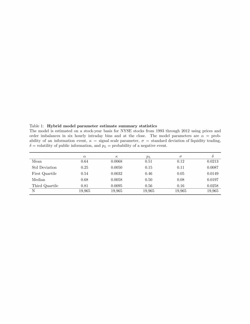
Table 1 reports summary statistics of the parameter estimates for the panel of firm-years
(summary statistics by year are plotted in Figure 7 in Section 3.5). To see which aspects
of the data determine the parameter estimates, Table 2 reports regressions of the parameter
estimates on various moments of order flows and returns. The table also reports variance
decompositions. The moments include correlations of order flows and returns split into two
subperiods of the day—the first three hours and the last three and a half hours. The price
function in the model is nonlinear, so we also include nonlinear measures of the comovement
of returns and order imbalances. Specifically, we include correlations of returns with squared
order imbalances for the two subperiods. We also include the fraction of the days on which
returns and order imbalances are both in the right tails of their distributions and the fraction
in which they are both in their left tails, defining a tail as a standard deviation away from
zero (a zero order imbalance or a zero rate of return).
The R-squareds and the variance decomposition show that the estimates of the stan-
dard deviation σ of order imbalances from the model are almost entirely determined by the
empirical standard deviations of order imbalances. Likewise, the estimates of the volatility
δ of the public news process are almost entirely determined by the standard deviations of
returns. The private information parameters κ, α and pL are naturally more complex.
The moments have little explanatory power for the pL estimates, though it is natural that
skewness of returns and order flows matter for this parameter. The non-linear comovement
measures are also related to pL. As shown in Table 1, the distribution of the pL estimates is
fairly tight around 50%, so there is not too much variation to explain.
The κ and α estimates are the most interesting. The magnitude κ of private information is
fairly well explained by the moments, with the most important moments being the standard
17
deviation of returns and the correlations between order imbalances and returns. The variance
decomposition shows that all of the moments except skewness affect the estimated probability
α of information events. The nonlinear specification is important for α. Almost two-thirds
of the R-squared comes from the correlations and the right and left tail variables.
3.2. Testing Whether There is Always an Information Event in the Hybrid Model
Our hybrid model relaxes the assumption in Kyle (1985) that an information event occurs
in each instance of the model (in each day in our implementation). A natural question is
whether this relaxation is supported in the data. The Kyle framework is nested in our model
by the restriction that α = 1. Accordingly, we estimate the model with this restriction. The
standard likelihood ratio test of the null that α = 1 against the alternative that α ∈ [0, 1] is
rejected for 73% of the firm-years (with a test size of 10%). However, the usual regularity
conditions for the likelihood ratio test require that the restriction not be at the boundary of
the parameter space. To address this issue, we bootstrap the distribution of the likelihood
ratio statistic for a random sample of 100 firm-years as in Duarte and Young (2009).
Specifically, for a given firm-year, we estimate the restricted model (α = 1) and then
simulate 500 firm-years under the null using the estimated (restricted) parameters. We then
estimate the restricted and unrestricted models for each simulated firm-year to obtain the
distribution of the likelihood ratio under the null. The 90th percentile of this distribution is
the critical value to evaluate the empirical likelihood ratio. These bootstrapped likelihood
ratio tests reject the restricted Kyle model in favor of the hybrid model for 62 of the 100
randomly selected firm-years. The data thus supports the conclusion that the probability of
an information event is less than 1.
3.3. Estimated Parameters and Reduced-Form Price Impacts
The model places structure on the price and order flow data, allowing the econometrician
to identify components of Kyle’s lambda. Of course, one can estimate a reduced-form price
impact as well. As an initial test of whether our estimates relate to price impact as implied
18
by theory, we test the comparative statics from Figure 2 that price impacts are increasing
in both the probability and magnitude of information events.
We employ three estimates of the price impact of orders. The first is the 5-minute percent
price impact of a given trade k as:
5-minute Price Impactk =2Dk(Mk+5 −Mk)
Mk
, (11)
where Mk is the prevailing quote midpoint for trade k, Mk+5 is the quote midpoint five min-
utes after trade k, and Dk equals 1 if trade k is a buy and −1 if trade k is a sell. Goyenko,
Holden and Trzcinka (2009) use this measure as one of their high-frequency liquidity bench-
marks in a study assessing the quality of various liquidity measures based on daily data.18
For a given stock-day, the estimate of the percent price impact is the equal-weighted average
price impact over all trades on that day. We average these daily price impact estimates for
each stock-year.
We also estimate the cumulative impulse response function (Hasbrouck, 1991), which
captures the permanent price impact of an order. The cumulative impulse response is cal-
culated from a vector autoregression of log price changes and signed trades. Finally, we
estimate a version of Kyle’s lambda (denoted λintraday) using a regression of 5-minute returns
on the square-root of signed volume following Hasbrouck (2009) and Goyenko, Holden and
Trzcinka (2009). We estimate these for each stock day, taking the median estimate across
days as the stock-year estimate.
The first panel of Table 3 reports panel regressions of the three price impact measures on
the hybrid model parameters that measure private information (the probability α of an in-
formation event and the magnitude κ of information events). Before running the regressions,
the price impacts and the structural parameters are winsorized at 1/99% and standardized
18Holden and Jacobsen (2014) show that liquidity measures such as the percent price impact can be biasedwhen constructed from monthly TAQ data, so we follow their suggested technique in processing the data.
19
to have unit standard deviations. Price impacts are positively related to both α and κ. The
coefficients are positive even with the inclusion of firm fixed effects, indicating that α and κ
capture within-firm information asymmetry variation as well.
A summary measure of the amount of private information is the standard deviation of
the signal ξS, denoted SD(ξS), which equals
2κ√αpL(1− pL) . (12)
The second panel of Table 3 shows that the estimated SD(ξS) is strongly positively correlated
with the price impact estimates, as expected. Cross-sectionally, a one standard deviation
increase in SD(ξS) is associated with around three-quarters of a standard deviation increase
in 5-minute price impact and λintraday and about half a standard deviation increase in the cu-
mulative impulse response measure. Variation in SD(ξS) within firm is positively correlated
with within-firm variation in all three price impact measures.
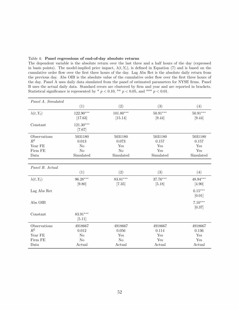
3.4. Kyle’s Lambda and Stochastic Volatility
In the model, prices evolve as dPt = dVt +λ(t, Yt) dYt. The changing sensitivity of prices
to order flows means that prices exhibit stochastic volatility. In Table 4, we investigate
this implication of the model for simulated and actual data. Volatility is measured as the
absolute return over the last three and a half hours of the trading day. We calculate λ(t, Yt)
from Equation (7) for each day using the cumulative order imbalance over the first three
hours of the day (i.e., t=3/6.5), along with the estimated parameters. We report predictive
regressions of volatility on λ(t, Yt).
The top panel of Table 4 reports results for a simulated panel created by generating 252
days for each set of parameter estimates. Higher levels of λ(t, Yt) predict higher volatility
in the second part of the day. The bottom panel shows that this phenomenon holds in the
actual data as well. Moreover, the magnitudes are similar across the simulated and actual
data controlling for firm and year fixed effects. Confidence intervals at standard significance
20
levels overlap across the simulated and actual data. Of course, in the actual data, other
phenomena could lead to stochastic volatility. In the last column, we control for the prior
day’s realized absolute return as well as the absolute cumulative order imbalance over the first
part of the day. λ(t, Yt) continues to predict volatility, and the magnitude of its coefficient
is quite similar to that in the simulated data.
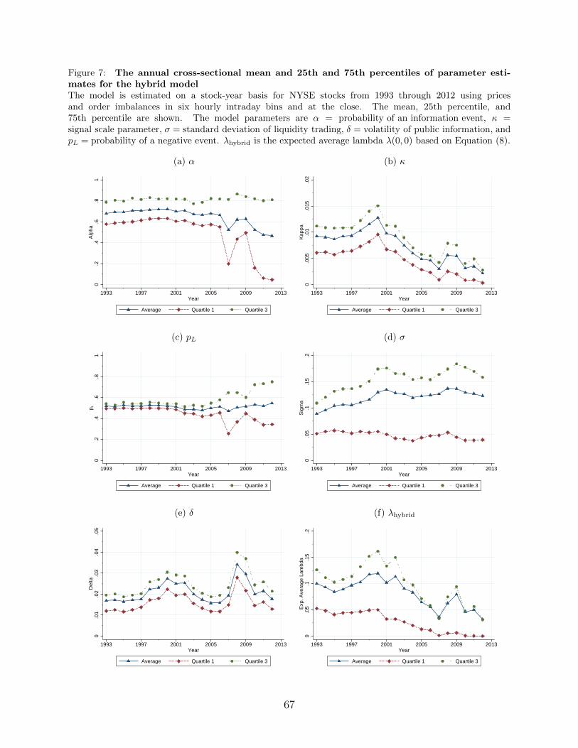
3.5. Time Series of Estimates
Figure 7 displays the time series of cross-sectional averages and interquartile ranges of the
parameter estimates. This supplements the summary statistics given for the panel in Table 1.
The average α is almost 70% in the early part of the sample and falls to about 50% by the end
of the sample. This effect starts in 2007 coincident with the introduction of the NYSE Hybrid
Market which increased automated electronic execution and increased execution speeds. It
is possible that market changes altered incentives to pursue private information, resulting in
lower α estimates. Hendershott and Moulton (2011) find that prices became more efficient
following the roll-out of the Hybrid Market, which aligns with a reduced probability of private
information events.19 The other components of private information events are the magnitude
κ of the signal and the likelihood pL of a bad event. The κ estimates initially rise during the
late 1990s but exhibit a strong downward trend thereafter. The average pL indicates that
the distribution of information is relatively symmetric between positive and negative events.
We combine these estimates into a single composite measure of information asymmetry by
calculating the expected average lambda from Equation (8). The estimates of this composite
measure indicate that the amount of private information has fallen across the twenty-year
sample with the exception of the late 1990s and the financial crisis.20
In general, the standard deviation σ of order imbalances and the volatility δ of public
19In untabulated results, we find that the decline in α starting in 2007 is more pronounced for largerfirms. Algorithmic traders (including high-frequency traders) disproportionately trade in large stocks, so itis unsurprising that the increased automation and execution speed of the Hybrid Market affected large firmsmore than small firms.
20As we discuss in Section 5.3, the same pattern is seen in reduced-form price impact measures.
21
information appear to be roughly stationary. Despite the well-documented rise of high-
frequency trading and the associated sharp increase in trading volume, the volatility of order
imbalances has remained fairly stable over the twenty-year sample. Like private information,
public information volatility also spiked during the financial crisis. This suggests private
information may be proportional to public information rather than a fixed amount.
4. Applications
We now discuss potential applications of the estimation procedure. A large literature
uses the PIN model, as discussed previously. Broadly speaking, some of this work relates
PIN estimates to times when researchers believe information events have likely occurred.
Other research uses PIN to proxy for information asymmetry or price informativeness. We
discuss examples of how our estimates might be useful to research of either type.
4.1. Detecting Information Events
Information asymmetry is generally unobservable, so testing performance of adverse se-
lection measures is challenging. In this subsection, we study how the conditional probability
of an information event as measured by our model varies in two settings considered in the
literature: earnings announcements and trading by Schedule 13D filers.
4.1.1. Earnings Announcements
Many studies have examined the information environment surrounding earnings an-
nouncements. Some studies assume that information asymmetry is higher prior to infor-
mation events, while others note that private ability or knowledge to interpret public infor-
mation may result in adverse selection following announcements (Kim and Verrecchia, 1997).
Several recent papers (Duarte et al., 2016; Brennan et al., 2016) use conditional estimates
based on the PIN and OWR models around earnings announcements.
As we discuss in Section 2.1, one can assess the probability of an information event if
one observes cumulative order flows and knows the underlying parameters. In particular,
22
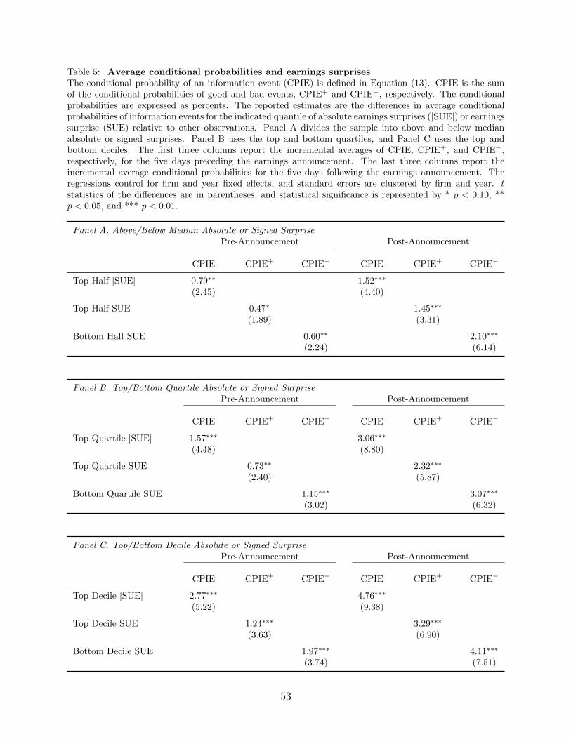
Theorem 1 shows that market makers update their conditional probabilities of an information
event, CPIE t, as:
CPIE t(Yt) =
N(yL−Ytσ√
1−t
)+ N
(Yt−yHσ√
1−t
)if t < 1 ,
1 (Y1 < yL) + 1 (Y1 > yH) if t = 1 .
(13)
Armed with our estimates of the parameters, we examine end-of-day conditional probabilities
of an information event, CPIE1, on the days around earnings announcements. We also
calculate conditional probabilities of positive and negative information events, CPIE+ and
CPIE−, respectively, which are the two components of CPIE in (13).
Figure 8 plots the cross-sectional average of model-implied CPIE in event time around
earnings announcements. The average CPIE rises significantly on day t− 1, consistent with
early leakage of some information prior to the announcement. The average CPIE is highest
on days t and t+ 1, and then falls over the next week or so. The results suggest that adverse
selection may actually be worse following an earnings announcement rather than before it,
as discussed in Kim and Verrecchia (1997).21
Pre-announcement information asymmetry is likely higher when a firm experiences an
earnings surprise. To test whether CPIE captures this, we use data from IBES to calculate
standardized unexpected earnings, SUE, calculated as
SUEt =EPSactual,t − EPSmedian forecast,t
Pt, (14)
where EPSmedian forecast,t is the median analyst forecast in the 90 days prior to the earnings
announcement. We expect there to be more informed trading when the absolute value of SUE
is higher. Moreover, the informed trading should correspond to the subsequent direction of
the earnings surprise. That is, higher (lower) signed earnings surprises should correspond to
21This conclusion is also reached by Krinsky and Lee (1996) using the adverse selection component ofbid-ask spreads and by Brennan et al. (2016) using conditional probabilities from the PIN model.
23
higher CPIE+ (CPIE−) preceding announcements. The first three columns of Table 5 show
that this is indeed the case. The average conditional probability of an information event in
the five days preceding announcements is 80 bps higher for above median |SUE| observations
relative to below median magnitude surprises. The average CPIE preceding earnings where
the |SUE| is in the top decile is almost 3% higher than the average across smaller earnings
surprise events. Table 5 shows that the direction of the surprises also corresponds to positive
or negative event probabilities. Average CPIE+ is higher before more positive SUE events,
and average CPIE− is higher preceding more negative SUE events.
Greater amounts of new information also increase the likelihood that asymmetrically-
informed investors can trade advantageously following an announcement (Kim and Verrec-
chia, 1997). If this is the case, we expect larger magnitude |SUE| to be correlated with
informed trading in the post-announcement period. Column four of Table 5 confirms that
this is the case. In the five days following announcements, CPIE is higher for larger mag-
nitude surprises. Moreover, the differences are larger than those in the pre-announcement
period, again suggesting that there is more informed trading following earnings announce-
ments than preceding them. The well-known post-earnings announcement drift suggests that
private information is often in the same direction of the earnings surprise. Consistent with
this, the final two columns of Table 5 show that average CPIE+ is higher following more
positive surprises, while average CPIE− is higher following the most negative surprises.
4.1.2. Schedule 13D Filings
Collin-Dufresne and Fos (2015) examine whether various measures of adverse selection are
higher during periods in which Schedule 13D filers accumulate ownership positions. These
positions are generally associated with a positive stock price reaction, so these investors are
privately informed. These investors must disclose days on which they traded over a sixty-
day period preceding the filing date. Thus, this data provides the econometrician with a
laboratory concerning informed trading. Collin-Dufresne and Fos (2015) show that measures
designed to capture information asymmetry are actually lower on days when Schedule 13D
24
filers trade. As they discuss, this could be due to endogenous trading in times of greater
liquidity and due to the use of patient limit orders. The latter effect arises in part because
of the filers’ ability to control the timing of the private information revelation. This differs
from the pre-earnings announcement setting where an informed trader’s information is valid
only for an exogenous duration.
We revisit the Schedule 13D setting to assess whether the conditional probability of an
information event is higher on days when these informed investors trade. According to our
model, there are informed trades on days when there are information events. So, we regard
the days on which 13D filers trade as information event days. Consistent with this, Collin-
Dufresne and Fos (2015) show that days when Schedule 13D filers trade are characterized
by significant market-adjusted returns. 13D filers typically accumulate shares by trading on
occasional days over a period of weeks. Over the sixty-day disclosure window, the probability
that a Schedule 13D filer trades on a given day ranges from around 25% to 50% (Collin-
Dufresne and Fos, 2015, Figure 1). One potential reason for trading on particular days
is news that causes revisions in estimates of the value of activism. If activists are better
informed than the market about such valuation revisions, which is quite likely, these events
fit our model of private information.22
Table 6 reports average values of CPIE on days during the sixty-day disclosure window
when Schedule 13D filers do or do not trade. Just under two-thirds of the firm-days with
no Schedule 13D trades are identified as being event days. On the other hand, 70% of the
days when Schedule 13D filers do trade are identified as event days. The increase of 7.8%
is statistically significant and represents about a 13% increase in the conditional probability
relative to non-13D trading days. Thus, despite the fact that trading by Schedule 13D filers
is inversely correlated with the various measures of permanent price impact commonly used
22Another reason that 13D filers may choose to trade on particular days is that liquidity trading may betime varying. This reason is proposed by Collin-Dufresne and Fos (2015). We could accommodate that byallowing σ to be time varying, but that extension is beyond the scope of the paper. Our goal here is to showthat our current model, with constant σ, is informative about trading by 13D filers.
25
in the literature and employed by Collin-Dufresne and Fos (2015), we find that the trading by
13D filers is manifested in higher conditional probabilities of an information event, calculated
according to our model.
We also report average CPIE for two subperiods, the first and second halves of the dis-
closure period (days [t − 60, t − 31] and [t − 30, t − 1], respectively). If block accumulation
by a 13D filer is detected by other strategic traders, then both the 13D filer and the other
strategic traders should trade aggressively to beat others to the market (Holden and Sub-
rahmanyam, 1992). This is more likely to have occurred during the second subperiod, so
we expect Schedule 13D filers to trade more aggressively (use more market orders rather
than limit orders) in the second subperiod. Furthermore, the second subperiod includes the
period after crossing the 5% threshold, after which the 13D must be filed within ten days.
We certainly expect more aggressive trading during that period. As a result of these consid-
erations, we expect signed order flow to reflect the presence of informed trade more in the
second subperiod than in the first. The second and third rows of Table 6 show that this is
indeed the case. There is a smaller difference of 5.3% in CPIE over the first 30 days of the
block-accumulation period between Schedule 13D trading days and non-trading days. In the
second half of the disclosure period however, the average CPIE is 9.2% higher on days when
informed Schedule 13D filers trade than on days they do not.
4.2. Measuring the Information Content of Prices
Some studies use PIN to measure the information content of prices in order to test
various economic theories. Applications in corporate finance include Chen, Goldstein and
Jiang (2007), Ferreira and Laux (2007), and Bharath, Pasquariello and Wu (2009), and
applications in accounting include Frankel and Li (2004), Jayaraman (2008), and Brown and
Hillegeist (2007).
Here, we demonstrate how our structural estimates could be used to augment one such
study. Chen et al. (2007) study how corporate managers learn from prices in making invest-
ment decisions. They find that investment sensitivity to prices (Q) is increasing with price
26
informativeness as proxied by PIN and by 1−R2 from an asset pricing model. In Table 7, we
replicate Chen et al. (2007) for our sample. Before running the regressions, we standardize
each information environment variable to have unit standard deviation. As in Chen et al.
(2007), the coefficient on Q is increasing in PIN (column 2).
To demonstrate how researchers might employ our methodology in this setting, we con-
sider two composite measures of the information environment from the hybrid model. The
first is the standard deviation of the signal (SD(ξS)) from Equation (12). We also calcu-
late the proportion of the return variance due to private information, which we term the
order-flow component of prices (OFC):
var(ξS)
var(ξS) + var(eδBi1−δ2/2)=
SD(ξS)2
SD(ξS)2 + eδ2 − 1. (15)
Columns 4 and 5 of Table 7 show that investment-price sensitivity is increasing in each of
these measures.
One advantage of our estimation procedure relative to PIN is that it allows us to sepa-
rately estimate the probability and magnitude of information events. Investment sensitivity
to prices is increasing in each of these components (column 6 of Table 7). Thus, when there
are more frequent or larger episodes of private information, investment is more sensitive to
prices. A one standard deviation increase in κ (the magnitude of information events) is
associated with about a 25% increase in investment-price sensitivity. A standard deviation
change in α (the probability of an information event) has an effect about two-thirds as large.
The positive effect of α conflicts with results from decomposing PIN into the probability of
an information event and the relative intensity of liquidity to informed traders (column 3).
An increase in the PIN α does not lead to increased investment sensitivity to prices.
4.3. Probability and Magnitudes of Private Information
Estimation of the probability and magnitude of information events could also prove use-
ful in other settings where researchers are interested in the information environment. For
27
instance, the estimates can provide additional texture to studies of the effects of information-
related regulation such as insider trading laws, short-selling restrictions, or symmetric access
to managers for financial analysts (e.g., Reg FD in the US). Separating the probability and
magnitude of information events could be useful in the analyst literature more broadly. Do
analysts turn private information into public information? If so, one might expect to see
lower probabilities of information events for firms with greater analyst coverage. On the
other hand, analysts may produce private information, which could result in higher prob-
abilities of information events. Studies interested in how the investor base affects liquidity
could be more nuanced by including both α and κ. Index inclusion affects institutional own-
ership, so how does index inclusion affect the information environment? Greater institutional
ownership could result in lower magnitudes of private information if prices are more efficient
with institutional ownership. The accounting literature considers whether disclosure quality
and frequency affect the information environment of firms. Greater disclosure quality could
reduce the magnitude of private information, and greater disclosure frequency could reduce
the probability of private information events. In all of these cases, studying both α and κ
could improve our understanding relative to studying only composite measures of private
information.
5. Comparison to Other Models
In this section, we compare the estimates of our model to those of the three structural
models (PIN, APIN, OWR) and the reduced-form version of PIN (VPIN) discussed in the
introduction. The estimation procedure for the other models is detailed in Internet Appendix
C.
5.1. Correlations of Model Parameters
Panel A of Table 8 shows the correlations among PIN, APIN, VPIN, lambda from the
OWR model (λOWR), and the expected average lambda from our model (λhybrid) – see Equa-
tion (8). All of the correlations are positive. The largest correlations with λhybrid are those
28
of the OWR lambda and VPIN. This is perhaps not surprising since each of these estimates
uses price changes in some form. The OWR lambda uses the joint distribution of returns
and order flows, while VPIN signs volume using price changes.
We call PIN, APIN, VPIN, λowr, and λhybrid composite measures of information asym-
metry because, with the exception of VPIN, they are functions of the underlying structural
parameters.23 We also examine the correlations of the structural parameters of the various
models. Panel B of Table 8 reports correlations of the estimated probability of an informa-
tion event from each model (except VPIN which does not identify α). The estimates of α
for the hybrid model are negatively correlated with estimates of α from the other models.
In each of the other models, the unconditional distribution of order flow imbalances changes
with α, unlike in our model, so the lack of correlation of the hybrid model α with the other
α’s is consistent with the identification discussion in Section 2.1. The implications of the
models for the unconditional distribution of order flow imbalances are discussed further in
Internet Appendix D.24
The positive correlation of λhybrid with the other composite measures is somewhat sur-
prising given that the α of the hybrid model is not positively correlated with the α’s of the
other models. The explanation lies in the estimates of liquidity trading. Equation (8) shows
that the expected average lambda is inversely related to the volatility of liquidity trading.
The other measures are also inversely related to liquidity trading (see Equations C.2, C.4,
and C.6 in the Internet Appendix). Panel C of Table 8 reports correlations of the liquidity
trading parameters of each model. We scale the PIN and APIN liquidity trading parameters
by the estimated µ, so the fractions ε/µ and (ε + θη)/µ represent the intensity of liquid-
ity trading relative to informed trading. Note that PIN and APIN are decreasing in these
23We refer to VPIN as reduced-form because it does not identify the underlying structural parameters.Rather, it proxies for PIN by separately estimating the numerator and denominator of PIN—see InternetAppendix C.4.
24Venter and de Jongh (2006), Duarte and Young (2009), Gan, Wei and Johnstone (2014), and Duarte,Hu and Young (2016) all show that the PIN model fails to fit the empirical joint distribution of buy and sellorders.
29
ratios, respectively. The liquidity trading parameters are positively correlated across the
models. For this reason, the composite measures are positively correlated despite the lack of
correlation of the estimated alphas.
5.2. Cross-Sectional Variation in Parameters
It is interesting to see how estimates of private information differ in the cross-section of
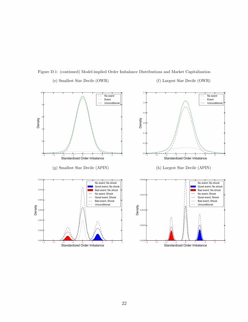
firms across models. Table 9 reports average values of the estimates within market capi-
talization deciles. Across all of the models, composite measures of information asymmetry
decrease in firm size (Panel A). For the hybrid model, the average probability α of an in-
formation event decreases in firm size while the estimates for the other models are exactly
the opposite, increasing in firm size (Panel B). As in the unconditional correlation analysis,
the composite measures seem to behave similarly in the size cross section due to similarities
in liquidity trading measurement (Panel C). Estimates from all of the models indicate more
intense liquidity trading for larger capitalization stocks. For each of the models other than
the hybrid model, the effect of the more pronounced liquidity trading dominates the modest
increases in α as a function of size, so these composite measures are lower for larger firms as
a result of higher estimated liquidity trading.25
5.3. Relation to Price Impacts and Quoted Spreads
In theory, price impacts and quoted spreads should be larger when information asym-
metry is higher. This is shown in Section 2 for price impacts in the hybrid model. For
the PIN model, the opening quoted spread is the product of PIN and the magnitude of the
information, H − L.26 In this section, we assess how time-series and cross-sectional varia-
tions in price impacts and quoted spreads relate to the estimated composite measure from
each model. For price impacts, we use the three measures described in Section 3.3. Quoted
25The OWR lambda is also a function of its estimated magnitude of private information σi. For both thehybrid model and the OWR model, the estimated magnitude of private information is also decreasing insize.
26See Equation (11) of Easley et al. (1996), which assumes pL = pH .
30
spreads are the time-weighted average proportional bid-ask spreads.
Figure 9 plots the time series of the cross-sectional averages and interquartile ranges of
the price impact measures, the quoted spread, and the five composite information asymmetry
measures. Over the twenty year sample, price impacts initially rose over the 1990s before
falling dramatically following the turn of the century, with the brief exception of the financial
crisis. Quoted spreads have also fallen over the sample period. Note that the time-series of
the hybrid model expected average lambda, λhybrid, and the magnitude of private information,
κ, exhibit similar patterns (Figure 7). The OWR lambda also exhibits similar behavior. PIN,
APIN, and VPIN are much less variable over time.
Table 10 explores the time-series relationships across these measures more formally. For
each firm with at least five years of estimates, we calculate the time-series correlations be-
tween the price impact or quoted spread measure and each model-based composite measure.
Table 10 reports the cross-sectional average of these time-series correlations. For all three
reduced-form price impact estimates and for quoted spreads, λhybrid is the most correlated
composite measure and is significantly more correlated than the other composite measures.
Using the approximately 1600 firms with at least five years of estimates, paired t-tests reject
the nulls that the correlation with λhybrid equals the correlations with the other composite
measures (Panel B of Table 10).
We also explore how the composite measures relate cross-sectionally to the price impact
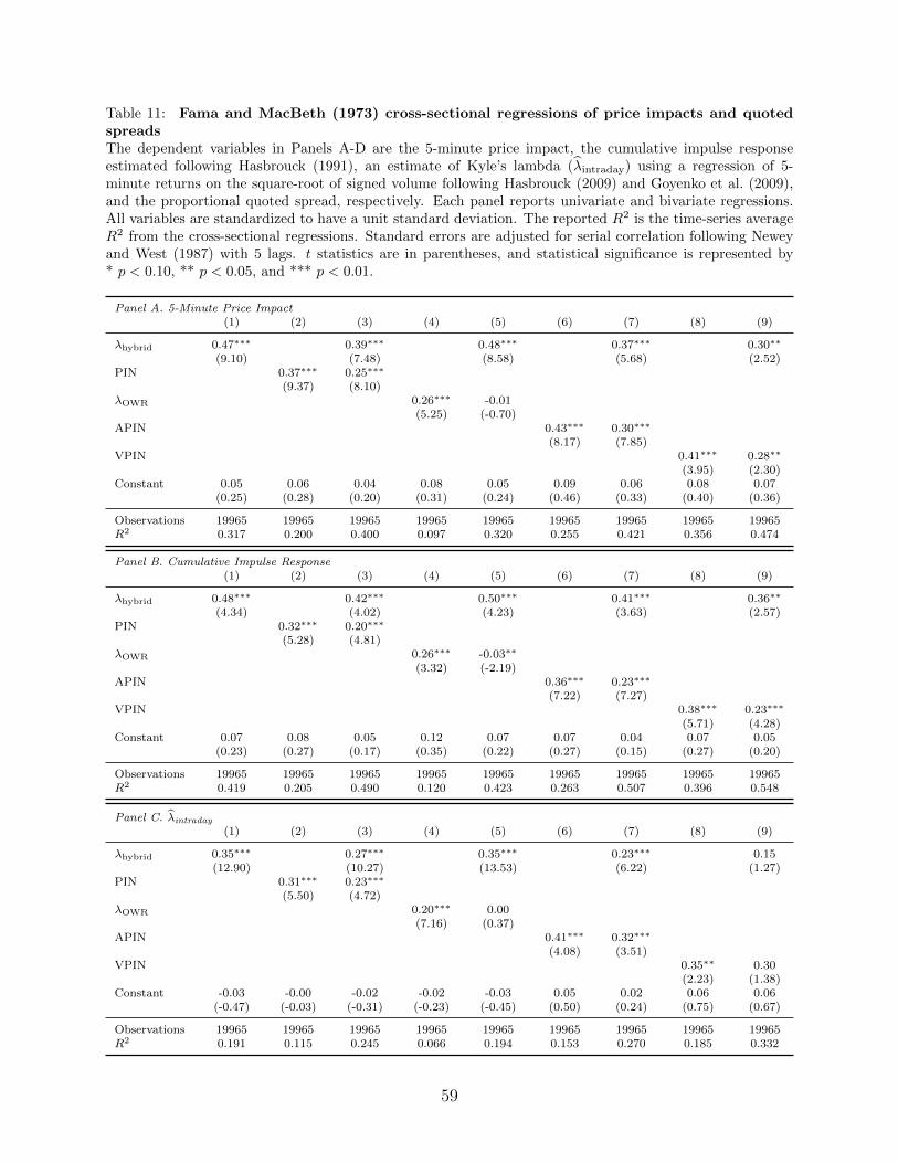
and quoted spread benchmarks. Table 11 reports cross-sectional regressions of price impacts
and quoted spreads on the composite information asymmetry measures. We run univariate
regressions as well as bivariate regressions including λhybrid and another composite measure.
The information asymmetry measures are standardized to have unit standard deviations. In
univariate regressions, the reduced-form price impact measures and quoted spreads are posi-
tively related to each of the information asymmetry measures. λhybrid generally explains the
most (or second-most) cross-sectional variation in price impacts and explains over a quarter
31
of the variation in quoted spreads.27 Perhaps more importantly, λhybrid adds explanatory
power to each of the other composite measures regardless of the benchmark when comparing
the bivariate and univariate regressions. This is true for both the price impact benchmarks
and for quoted spreads.
The hybrid model parameters are estimated using a sample of prices and order flows, so
it is perhaps unsurprising that λhybrid captures reduced-form price impacts well. However,
this critique does not apply to quoted spreads, which are not part of the data used in
the estimation. Tables 10 and 11 show that λhybrid also performs well vis-a-vis alternative
composite measures when quoted spreads are used as the benchmark.
Of course, there remains unexplained variation in both reduced-form price impacts and
quoted spreads. Some empirical work on information asymmetry has aggregated various em-
pirical proxies of information asymmetry to try to capture the multifaceted nature of liquidity
(e.g., Bharath et al., 2009; Korajczyk and Sadka, 2008). The fact that none of the compos-
ite measures, including λhybrid, completely explains price impacts or quoted spreads, lends
credence to such aggregations. Our results suggest that λhybrid or its underlying structural
parameters should be included when empirical researchers wish to aggregate information
asymmetry estimates.
6. Conclusion
We propose a model of informed trading that is a hybrid of the PIN and Kyle models.
Unlike the Kyle model, information events occur with probability less than one as in the
PIN model, and unlike the PIN model, informed orders are endogenously determined as in
the Kyle model. An important implication of the model is that both returns and order flows
are needed to identify information asymmetry parameters. The reason is that order flows
depend on market liquidity, which depends on information asymmetry. This is an indirect
27For the univariate quoted spreads regressions, VPIN has the largest average R2, but its coefficientestimate is insignificant. This is because VPIN and quoted spreads are negatively correlated cross-sectionallyover the first five years of the sample.
32
dependence of order flows on information asymmetry that is countervailing to the direct
relation. This result suggests that measures of information asymmetry based solely on order
flows (like PIN) may be misspecified.
We estimate the hybrid model and provide several analyses that suggest the estimates
capture cross-sectional and time-series variation in information asymmetry. We illustrate
possible applications of our estimates: a new methodology to detect information events and
a corporate finance application. Our model allows the econometrician to identify distinct
components of information asymmetry such as the probability and magnitude of potential
information events. We hope such refinements will prove useful to future finance and ac-
counting research.
Finally, we compare the parameter estimates to those from other structural models and to
price impacts and quoted spreads. While composite information asymmetry measures from
all of the models are positively correlated with price impacts, the measure from the hybrid
model exhibits higher time-series correlations and incremental cross-sectional explanatory
power for price impacts. To a certain extent, this might be expected, since the measure
from the hybrid model is the expected average Kyle’s lambda, and Kyle’s lambda should
be highly correlated with price impacts. However, the measure from the Odders-White and
Ready (2008) model is also an estimate of a Kyle’s lambda, and it is dominated by the
hybrid model in explaining both time-series and cross-sectional variation in price impacts.
Moreover, the hybrid model measure is also more correlated with quoted spreads than other
measures in the time series and adds explanatory power to each of the other measures in
explaining the cross-section of quoted spreads.
33
Appendix A. Proofs
The process Y described in the following lemma is a variation of a Brownian bridge. It
differs from a Brownian bridge in that the endpoint is not uniquely determined but instead is
determined only to lie in an interval—either the lower tail (−∞, yL), the upper tail (yH ,∞) or
the middle region [yL, yH ]—depending on whether there is an information event and whether
the news is good or bad. Part (C) of the lemma follows immediately from the preceding
parts, because the probability (A.3) is the probability that Y1 /∈ [yL, yH ] calculated on the
basis that Y is an FY –Brownian motion with zero drift and standard deviation σ.
Lemma. Let N denote the standard normal distribution function. Let FY = FYt | 0 ≤ t ≤
1 denote the filtration generated by the stochastic process Y defined by Y0 = 0 and
dYt =q(t, Yt, ξS)
1− t dt+ dZt . (A.1)
Then, the following are true:
(A) Y is an FY –Brownian motion with zero drift and standard deviation σ.
(B) With probability one,
ξ = 1 and S = L ⇒ Y1 < yL , (A.2a)
ξ = 0 ⇒ yL ≤ Y1 ≤ yH , (A.2b)
ξ = 1 and S = H ⇒ Y1 > yH . (A.2c)
(C) For each t < 1, the probability that ξ = 1 conditional on FYt is
N
(yL − Ytσ√
1− t
)+ 1− N
(yH − Ytσ√
1− t
). (A.3)
34
Proof of the Lemma. Set
k(1, y, s) =
1y<yL if s = L ,
1yL≤y≤yH if s = 0 ,
1y>yH if s = H ,
and, for t < 1,
k(t, y, s) =
N(yL−yσ√
1−t
)if s = L ,
N(yH−yσ√
1−t
)− N
(yL−yσ√
1−t
)if s = 0 ,
N(y−yHσ√
1−t
)if s = H .
Define
`(t, y, s) =∂ log k(t, y, s)
∂y,
for t < 1. Then, (1 − t)σ2`(t, y, s) = q(t, y, s) for t < 1, and the stochastic differential
equation (A.1) can be written as
dYt = σ2 `(t, Yt, ξS) dt+ dZt (A.4)
The process Y is an example of a Doob h-transform—see Rogers and Williams (2000).
To put (A.4) in a more standard form, define the two-dimensional process Yt = (ξS, Yt)
with random initial condition Y0 = (ξS, 0), and augment (A.4) with the equation d(ξS) = 0.
The existence of a unique strong solution Y to this enlarged system follows from Lipschitz
and growth conditions satisfied by `. See Karatzas and Shreve (1988, Theorem 5.2.9).
The uniqueness in distribution of weak solutions of stochastic differential equations
(Karatzas and Shreve, 1988, Theorem 5.3.10) implies that we can demonstrate Properties
(A) and (B) by exhibiting a weak solution for which they hold. To construct such a weak
35
solution, define a new measure Q on F1 using k(1, Z1, ξS)/k(0, 0, ξS) as the Radon-Nikodym
derivative. The definition of k implies that k(t, Zt, ξS) is the Ft–conditional expectation of
the indicator function k(1, Z1, ξS), so k(t, Zt, ξS) is a martingale on the filtration F. By
Girsanov’s Theorem, the process Z∗ defined by Z∗0 = 0 and
dZ∗t = −σ2 `(t, Zt, ξS) dt+ dZt
is a Brownian motion (with zero drift and standard deviation σ) on the filtration F relative
to Q. It follows that Z is a weak solution of (A.4) relative to the Brownian motion Z∗ on
the filtered probability space (Ω,F,Q).
To establish Property (A) for the weak solution, we need to show that Z is a Brownian
motion on (Ω,G,Q). Because Z is a Brownian motion on (Ω,G,P), it suffices to show that
Q = P when both are restricted to G1. This holds if for all t1 < · · · < tn ≤ 1 and all Borel
using the fact that J(1, y, s) ≥ 0 for all (y, s) for the inequality. Thus, E[J(0, 0, ξS)] is an
upper bound on the expected profit, and the bound is achieved if and only if J(1, Y1, ξS) = 0
with probability one. By the definition of J(1, y, s), this is equivalent to Y1 < yL with
probability one when ξS = L, yL ≤ Y1 ≤ yH with probability one when ξ = 0, and Y1 > yH
with probability one when ξS = H. By part (B) of the proposition, the strategy (5) is
therefore optimal.
Proof of Theorem 2. By Ito’s formula and the fact that (dY )2 = (dZ)2 = σ2 dt, we have
dp(t, Yt) =
(pt(t, Yt) +
1
2σ2pyy(t, Yt)
)dt+ py(t, Yt) dYt ,
where we use subscripts to denote partial derivatives. Both Y and p(t, Yt) are martingales
with respect to the market makers’ information, so the drift term must be zero. That can
also be verified by direct calculation of the partial derivatives, using the formula (6) for
40
p(t, y). Thus,
dp(t, Yt) = py(t, Yt) dYt .
A direct calculation based on the formula (6) for p(t, y) shows that py(t, y) = λ(t, y) defined
in (7).
To see that λ(t, Yt) is a martingale for t ∈ [0, 1), with respect to market makers’ infor-
mation, we can calculate, for t < u < 1,
E[λ(u, Yu) | Yt = y] = − L
σ√
1− u ·∫ ∞−∞
n
(yL − y′σ√
1− u
)f(y′ | u− t, y)dy′
+H
σ√
1− u ·∫ ∞−∞
n
(yH − y′σ√
1− u
)f(y′ | u− t, y)dy′ ,
where f(· | τ, y) denotes the normal density function with mean y and variance σ2τ . A
straightforward calculation shows that this equals λ(t, y). For example, to evaluate the first
term, use the fact that
1
σ√
1− u n
(yL − y′σ√
1− u
)f(y′ | u− t, y)
=1
σ√
1− t n
(yL − yσ√
1− t
)× 1√
2πσ2(1− u)(u− t)/(1− t)
× exp
(−(
1− t2(1− u)(u− t)σ2
)(y′ − (1− u)y + (u− t)yL
1− t
)2),
which integrates to
1
σ√
1− t n
(yL − yσ√
1− t
),
because the other factors constitute a normal density function.
41
Appendix B. Hybrid Model Likelihood Function
Assume the trading period [0, 1] corresponds to a day. This implies that any private
information becomes public before trading opens on the following day.28 We can estimate
the model parameters using intraday price and order flow information. If we assume further
that the model parameters are stable over time, then the price and order flow information
from multiple days can be merged to estimate the parameters with greater precision.
To obtain stationarity in returns, assume that the possible signal realizations on each
day are proportional to the observed opening price. Specifically, on each day i, assume that
the possible signal realizations are
Li = 2(pL − 1)κPi0 ,
Hi = 2pLκPi0 ,
where Pi0 denotes the opening price on day i and where κ is a parameter to estimated.
With this specification, the signal on each day has a zero mean, and (Hi − Li)/Pi0 = 2κ.
Thus, κ measures the signal magnitude. Denote the pricing function on day i (as specified
in Theorem 1) by pi(t, y), and let p(t, y) denote the pricing function when the possible signal
realizations are L = 2(pL − 1)κ and H = 2pLκ. Then, pi(t, y)/Pi0 = p(t, y).
The price at time t on day i is Vit + pi(t, Yit), and in particular the opening price is
Pi0 = Vi0, so the gross return through time t is
PitPi0
=VitVi0
+pi(t, Yit)
Pi0=VitVi0
+ p(t, Yit) . (B.1)
28In contrast to Odders-White and Ready (2008), our estimation does not use overnight returns. In ourtheoretical model, private information that is made public at the close of trading is incorporated into pricesbefore trading ends (convergence to strong-form efficiency). Thus, overnight returns in our model are dueto arrival of new public information, which does not aid in estimating the model.
42
Assume
dVitVit
= δ dBit
for a constant δ and a Brownian motion Bi, so we have
PitPi0
= p(t, Yit) + eδBit−δ2t/2 .
Assume the price and order imbalance are observed at times t1, . . . , tk+1 each day with
tk+1 = 1 being the close and the other times being equally spaced: tj = j∆ for ∆ > 0 and
j ≤ k. Let Pij denote the observed price and Yij the observed order imbalance at time tj on
date i. Let Γ denote the (k+1)–dimensional vector defined by Γj = tj/∆ for j = 1, . . . , k+1.
Let Σ denote the (k + 1)× (k + 1) matrix defined by Σjj′ = min(Γj,Γj′).
Let Ui denote the vector of log pricing differences as defined in (10). The density function
of (Pi1/Pi0, . . . , Pi,k+1/Pi0) conditional on Yi is
f(Ui1, . . . Ui,k+1)e−∑k+1
j=1 Uij ,
where f denotes the multivariate normal density function with mean vector −(δ2∆/2)Γ and
covariance matrix δ2∆Σ. Furthermore, on each day i, the vector Yi = (Yi,t1 , . . . , Yi,tk+1)′ is
normally distributed with mean 0 and covariance matrix σ2∆Σ.
Let Li denote the log-likelihood function for day i. Dropping terms that do not depend
on the parameters, we have
− Li = (k + 1) log σ +1
2σ2∆Y ′i Σ
−1Yi + (k + 1) log δ
+1
2δ2∆
(Ui +
δ2∆
2Γ
)′Σ−1
(Ui +
δ2∆
2Γ
)+
k+1∑j=1
Uij .
43
Using the facts that Γ′Σ−1 = (0, . . . , 0, 1) and Γ′Σ−1Γ = 1/∆, this simplifies to
− Li = (k + 1) log σ +1
2σ2∆Y ′i Σ
−1Yi + (k + 1) log δ
+1
2δ2∆U ′iΣ
−1Ui +1
2Ui,k+1 +
δ2
8+
k+1∑j=1
Uij .
Hence, the log-likelihood function L for an observation period of n days satisfies (9).
44
References
Akay, O., Cyree, K.B., Griffiths, M.D., Winters, D.B., 2012. What does PIN identify?Evidence from the T-bill market. Journal of Financial Markets 15, 29–46.
Akins, B., Ng, J., Verdi, R.S., 2012. Investor competition over information and the pricingof information asymmetry. The Accounting Review 87, 35–58.
Aktas, N., de Bodt, E., Declerck, F., Van Oppens, H., 2007. The PIN anomaly around M&Aannouncements. Journal of Financial Markets 10, 160–191.
Andersen, T., Bondarenko, O., 2014a. Reflecting on the VPIN dispute. Journal of FinancialMarkets 17, 53–64.
Andersen, T., Bondarenko, O., 2014b. VPIN and the flash crash. Journal of FinancialMarkets 17, 1–46.
Back, K., 1992. Insider trading in continuous time. Review of Financial Studies 5, 387–409.
Back, K., Baruch, S., 2004. Information in securities markets: Kyle meets Glosten andMilgrom. Econometrica 72, 433–465.
Banerjee, S., Breon-Drish, B., 2017. Dynamic information acquisition and strategic trading.Working Paper. University of California, San Diego.
Banerjee, S., Green, B., 2015. Signal or noise? Uncertainty and learning about whetherother traders are informed. Journal of Financial Economics 117, 398–423.
Benos, E., Jochec, M., 2007. Testing the PIN variable. Working Paper, University of Illinois.
Bharath, S.T., Pasquariello, P., Wu, G., 2009. Does asymmetric information drive capitalstructure decisions? Review of Financial Studies 22, 3211–3243.
Brennan, M.J., Huh, S.W., Subrahmanyam, A., 2016. High-frequency measures of informedtrading and corporate announcements. Working Paper,. UCLA.
Brown, S., Hillegeist, S.A., 2007. How disclosure quality affects the level of informationasymmetry. Review of Accounting Studies 12, 443–477.
Brown, S., Hillegeist, S.A., Lo, K., 2004. Conference calls and information asymmetry.Journal of Accounting and Economics 37, 343–366.
Brown, S., Hillegeist, S.A., Lo, K., 2009. The effect of earnings surprises on informationasymmetry. Journal of Accounting and Economics 47, 208–225.
Chakraborty, A., Yilmaz, B., 2004. Manipulation in market order models. Journal of Finan-cial Markets 7, 187–206.
Chen, Q., Goldstein, I., Jiang, W., 2007. Price informativeness and investment sensitivityto stock price. Review of Financial Studies 20, 619–650.
45
Collin-Dufresne, P., Fos, V., 2015. Do prices reveal the presence of informed trading? Journalof Finance 70, 1555–1582.
Duarte, J., Han, X., Harford, J., Young, L., 2008. Information asymmetry, informationdissemination and the effect of Regulation FD on the cost of capital. Journal of FinancialEconomics 87, 24–44.
Duarte, J., Hu, E., Young, L., 2016. What Does the PIN Model Identify as Private Infor-mation? Working Paper. Rice University and University of Washington.
Duarte, J., Young, L., 2009. Why is PIN priced? Journal of Financial Economics 91,119–138.
Easley, D., Hvidkjaer, S., O’Hara, M., 2002. Is information risk a determinant of assetreturns? Journal of Finance 57, 2185–2221.
Easley, D., Hvidkjaer, S., O’Hara, M., 2010. Factoring information into returns. Journal ofFinancial and Quantitative Analysis 45, 293–309.
Easley, D., Kiefer, N.M., O’Hara, M., Paperman, J.B., 1996. Liquidity, information, andinfrequently traded stocks. Journal of Finance 51, 1405–1436.
Easley, D., O’Hara, M., 2004. Information and the cost of capital. Journal of Finance 59,1553–1583.
Easley, D., Lopez de Prado, M., O’Hara, M., 2011. The microstructure of the “flash crash”:Flow toxicity, liquidity crashes, and the probability of informed trading. Journal of Port-folio Management 37, 118–128.
Easley, D., Lopez de Prado, M., O’Hara, M., 2012. Flow toxicity and liquidity in a high-frequency world. Review of Financial Studies 25, 1457–1493.
Easley, D., Lopez de Prado, M., O’Hara, M., 2014. VPIN and the flash crash: A rejoinder.Journal of Financial Markets 17, 47–52.
Fama, E.F., MacBeth, J.D., 1973. Risk, return, and equilibrium: Empirical tests. Journalof Political Economy 81, 607–636.
Ferreira, M.A., Laux, P.A., 2007. Corporate governance, idiosyncratic risk, and informationflow. Journal of Finance 62, 951–989.
Foster, F.D., Viswanathan, S., 1995. Can speculative trade explain the volume-volatilityrelation? Journal of Business & Economic Statistics 13, 379–396.
Frankel, R., Li, X., 2004. Characteristics of a firm’s information environment and the infor-mation asymmetry between insiders and outsiders. Journal of Accounting and Economics37, 229–259.
Gan, Q., Wei, W.C., Johnstone, D., 2014. Does the probability of informed trading modelfit empirical data? Working Paper.
46
Glosten, L.R., Harris, L.E., 1988. Estimating the components of the bid/ask spread. Journalof Financial Economics 21, 123–142.
Glosten, L.R., Milgrom, P.R., 1985. Bid, ask and transaction prices in a specialist marketwith heterogeneously informed traders. Journal of Financial Economics 14, 71–100.
Goldstein, I., Guembel, A., 2008. Manipulation and the allocational role of prices. Reviewof Economic Studies 75, 133–164.
Goyenko, R.Y., Holden, C.W., Trzcinka, C.A., 2009. Do liquidity measures measure liquid-ity? Journal of Financial Economics 92, 153–181.
Hasbrouck, J., 1988. Trades, quotes, inventories, and information. Journal of FinancialEconomics 22, 229–252.
Hasbrouck, J., 1991. Measuring the information content of stock trades. Journal of Finance46, 179–207.
Hasbrouck, J., 2009. Trading costs and returns for U.S. equities: Estimating effective costsfrom daily data. Journal of Finance 64, 1445–1477.
Hendershott, T., Moulton, P., 2011. Automation, speed, and stock market quality: TheNYSE’s hybrid. Journal of Financial Markets 14, 568–604.
Holden, C.W., Jacobsen, S., 2014. Liquidity measurement problems in fast, competitivemarkets: Expensive and cheap solutions. Journal of Finance 69, 1747–1785.
Holden, C.W., Subrahmanyam, A., 1992. Long-lived private information and imperfectcompetition. Journal of Finance , 247–270.
Hwang, L.S., Lee, W.J., Lim, S.Y., Park, K.H., 2013. Does information risk affect the impliedcost of equity capital? An analysis of PIN and adjusted PIN. Journal of Accounting andEconomics 55, 148–167.
Jayaraman, S., 2008. Earnings volatility, cash flow volatility, and informed trading. Journalof Accounting Research 46, 809–851.
Karatzas, I., Shreve, S.E., 1988. Brownian Motion and Stochastic Calculus. Springer-Verlag,New York.
Kim, O., Verrecchia, R.E., 1997. Pre-announcement and event-period private information.Journal of Accounting and Economics 24, 394–419.
Korajczyk, R.A., Sadka, R., 2008. Pricing the commonality across alternative measures ofliquidity. Journal of Financial Economics 87, 45–72.
Krinsky, I., Lee, J., 1996. Earnings announcements and the components of the bid-askspread. Journal of Finance 51, 1523–1535.
Odders-White, E.R., Ready, M.J., 2008. The probability and magnitude of informationevents. Journal of Financial Economics 87, 227–248.
Rogers, L.C.G., Williams, D., 2000. Diffusions, Markov Processes and Martingales: Vol. 2:Ito Calculus. 2nd ed., Cambridge University Press, Cambridge.
Rossi, S., Tinn, K., 2010. Man or machine? Rational trading without information aboutfundamentals. Working Paper.
Venter, J.H., de Jongh, D., 2006. Extending the EKOP model to estimate the probabilityof informed trading. Studies in Economics and Econometrics 30, 25–39.
Wang, Y., Yang, M., 2017. Insider trading when there may not be an insider. WorkingPaper. Duke University.
48
Table 1: Hybrid model parameter estimate summary statisticsThe model is estimated on a stock-year basis for NYSE stocks from 1993 through 2012 using prices andorder imbalances in six hourly intraday bins and at the close. The model parameters are α = prob-ability of an information event, κ = signal scale parameter, σ = standard deviation of liquidity trading,δ = volatility of public information, and pL = probability of a negative event.
Table 2: Hybrid model parameter estimates and moments of order flow and returnsThe dependent variables are the estimated parameters from the hybrid model. The explanatory variablesare various moments of order flows and returns. The unit of observation is a firm-year. OIB denotes thecumulative order flow over the full day. OIB1 and OIB2 are the order flows over the first 3 and last 3.5 hoursof the trading day. Similarly, R is the return over the full day, and R1 and R2 are returns over the first 3 andlast 3.5 hours of the trading day. The indicated moments of these variables are calculated across days foreach firm-year. # Right Tail OIB & R is the fraction of days where both OIB > sd(OIB) and R−1 > sd(R).# Left Tail OIB & R is the fraction of days where both OIB < −sd(OIB) and R − 1 < −sd(R). Panel Areports estimates where all variables are standardized to have a unit standard deviation. Standard errorsare clustered by firm and year. t statistics are in parentheses, and statistical significance is represented by* p < 0.10, ** p < 0.05, and *** p < 0.01. Panel B reports a variance decomposition. Each number in PanelB represents the fraction of the model’s total partial sum of squares corresponding to the moment in therow. The sum of each column is thus one.
Table 3: Panel regressions of price impactsThe independent variables are the estimated probability α of an information event, the magnitude κ of aninformation event (Panel A) and the standard deviation of the signal (SD(ξS)) (Panel B). The dependentvariables are the 5-minute price impact, the cumulative impulse response estimated following Hasbrouck(1991), and an estimate of Kyle’s lambda (λintraday) using a regression of 5-minute returns on the square-root of signed volume following Hasbrouck (2009) and Goyenko et al. (2009). All variables are standardizedto have a unit standard deviation. Standard errors are clustered by firm and year. t statistics are inparentheses, and statistical significance is represented by * p < 0.10, ** p < 0.05, and *** p < 0.01.
Panel A. Probability and Magnitude of Information Events
5-Minute Cumulative
Price Impact Impulse Response λintraday
(1) (2) (3) (4) (5) (6)
α 0.22∗∗∗ 0.09∗∗∗ 0.17∗∗∗ 0.06∗∗∗ 0.23∗∗∗ 0.12∗∗∗
(5.15) (4.00) (3.95) (2.93) (4.88) (4.13)
κ 0.58∗∗∗ 0.35∗∗∗ 0.42∗∗∗ 0.23∗∗∗ 0.67∗∗∗ 0.48∗∗∗
(16.03) (9.29) (9.86) (6.44) (10.74) (8.27)
Observations 19965 19965 19965 19965 19965 19965R2 0.591 0.800 0.625 0.829 0.369 0.642Year FE Yes Yes Yes Yes Yes YesFirm FE No Yes No Yes No Yes
Observations 19965 19965 19965 19965 19965 19965R2 0.635 0.823 0.655 0.842 0.438 0.679Year FE Yes Yes Yes Yes Yes YesFirm FE No Yes No Yes No Yes
51
Table 4: Panel regressions of end-of-day absolute returnsThe dependent variable is the absolute return over the last three and a half hours of the day (expressedin basis points). The model-implied price impact, λ(t, Yt), is defined in Equation (7) and is based on thecumulative order flow over the first three hours of the day. Lag Abs Ret is the absolute daily return fromthe previous day. Abs OIB is the absolute value of the cumulative order flow over the first three hours ofthe day. Panel A uses daily data simulated from the panel of estimated parameters for NYSE firms. PanelB uses the actual daily data. Standard errors are clustered by firm and year and are reported in brackets.Statistical significance is represented by * p < 0.10, ** p < 0.05, and *** p < 0.01.
Panel A. Simulated(1) (2) (3) (4)
λ(t, Yt) 122.90∗∗∗ 101.80∗∗∗ 50.91∗∗∗ 50.91∗∗∗
[17.63] [15.14] [9.44] [9.44]
Constant 121.30∗∗∗
[7.67]
Observations 5031180 5031180 5031180 5031180R2 0.013 0.073 0.157 0.157Year FE No Yes Yes YesFirm FE No No Yes YesData Simulated Simulated Simulated Simulated
Panel B. Actual(1) (2) (3) (4)
λ(t, Yt) 96.28∗∗∗ 83.81∗∗∗ 37.76∗∗∗ 48.94∗∗∗
[9.80] [7.35] [5.18] [4.90]
Lag Abs Ret 0.15∗∗∗
[0.01]
Abs OIB 7.10∗∗∗
[0.37]
Constant 83.91∗∗∗
[5.11]
Observations 4918667 4918667 4918667 4918667R2 0.012 0.056 0.114 0.136Year FE No Yes Yes YesFirm FE No No Yes YesData Actual Actual Actual Actual
52
Table 5: Average conditional probabilities and earnings surprisesThe conditional probability of an information event (CPIE) is defined in Equation (13). CPIE is the sumof the conditional probabilities of good and bad events, CPIE+ and CPIE−, respectively. The conditionalprobabilities are expressed as percents. The reported estimates are the differences in average conditionalprobabilities of information events for the indicated quantile of absolute earnings surprises (|SUE|) or earningssurprise (SUE) relative to other observations. Panel A divides the sample into above and below medianabsolute or signed surprises. Panel B uses the top and bottom quartiles, and Panel C uses the top andbottom deciles. The first three columns report the incremental averages of CPIE, CPIE+, and CPIE−,respectively, for the five days preceding the earnings announcement. The last three columns report theincremental average conditional probabilities for the five days following the earnings announcement. Theregressions control for firm and year fixed effects, and standard errors are clustered by firm and year. tstatistics of the differences are in parentheses, and statistical significance is represented by * p < 0.10, **p < 0.05, and *** p < 0.01.
Panel A. Above/Below Median Absolute or Signed SurprisePre-Announcement Post-Announcement
CPIE CPIE+ CPIE− CPIE CPIE+ CPIE−
Top Half |SUE| 0.79∗∗ 1.52∗∗∗
(2.45) (4.40)
Top Half SUE 0.47∗ 1.45∗∗∗
(1.89) (3.31)
Bottom Half SUE 0.60∗∗ 2.10∗∗∗
(2.24) (6.14)
Panel B. Top/Bottom Quartile Absolute or Signed SurprisePre-Announcement Post-Announcement
CPIE CPIE+ CPIE− CPIE CPIE+ CPIE−
Top Quartile |SUE| 1.57∗∗∗ 3.06∗∗∗
(4.48) (8.80)
Top Quartile SUE 0.73∗∗ 2.32∗∗∗
(2.40) (5.87)
Bottom Quartile SUE 1.15∗∗∗ 3.07∗∗∗
(3.02) (6.32)
Panel C. Top/Bottom Decile Absolute or Signed SurprisePre-Announcement Post-Announcement
CPIE CPIE+ CPIE− CPIE CPIE+ CPIE−
Top Decile |SUE| 2.77∗∗∗ 4.76∗∗∗
(5.22) (9.38)
Top Decile SUE 1.24∗∗∗ 3.29∗∗∗
(3.63) (6.90)
Bottom Decile SUE 1.97∗∗∗ 4.11∗∗∗
(3.74) (7.51)
53
Table 6: Average levels of the CPIE on days when Schedule 13D filers do or do not tradeThe conditional probability of an information event (CPIE) is defined in Equation (13). CPIE is expressedas a percent. The sample contains trading days in the sixty-day disclosure period prior to a Schedule 13Dfiling date for NYSE firms in the sample of Collin-Dufresne and Fos (2015). The first column reports theaverage CPIE on days when Schedule 13D filers trade. The second column reports the average CPIE ondays when Schedule 13D filers do not trade. The third column reports the differences between the two typesof days. We report the analysis for two subperiods, the first and second halves of the disclosure period (days[t − 60, t − 31] and [t − 30, t − 1], respectively). Standard errors are clustered by event. t statistics of thedifferences are in parentheses, and statistical significance is represented by * p < 0.10, ** p < 0.05, and ***p < 0.01.
Days with Days with NoInformed Trading Informed Trading Difference
(1) (2) (3)
Full Disclosure Window:Days [t− 60, t− 1]
CPIE 69.5 61.7 7.8∗∗∗
(4.86)
1st Half of Disclosure Window:Days [t− 60, t− 31]
CPIE 66.7 61.3 5.3∗∗
(2.35)
2nd Half of Disclosure Window:Days [t− 30, t− 1]
CPIE 71.2 62.0 9.2∗∗∗
(4.94)
54
Table 7: Panel regressions of corporate investmentThe dependent variable is capital expenditures. The independent variable Q is market-to-book of assets.PIN is the probability of informed trading from Easley et al. (1996). SD(ξS) is the standard deviation ofthe signal ξS as in Equation (12). OFC is the proportion of return variance due to private information (theorder-flow component of prices) as in Equation (15). α is the probability of an information event in either thePIN or hybrid model. κhybrid is the magnitude of an information event and σhybrid is the standard deviationof liquidity trading from the hybrid model. ε/µ is the ratio of the liquidity to informed trading intensitiesfrom PIN. Each information environment variable is standardized to have unit standard deviation. CF isfirm cash flows. RET is the cumulative return over the next three years. INV ASSET is the inverse of thebook value of assets. Standard errors are clustered by firm and year. t statistics are in parentheses, andstatistical significance is represented by * p < 0.10, ** p < 0.05, and *** p < 0.01.
Table 8: Correlations of structural parameters from the hybrid and other modelsFor all models, α = probability of an information event. For the hybrid model, λhybrid is the expectedaverage lambda λ(0, 0) based on Equation (8). PIN, APIN, and VPIN are the probabilities of informedtrading estimated using the methodologies in Easley et al. (1996), Duarte and Young (2009), and Easleyet al. (2012), respectively. λOWR is the estimate of Kyle’s lambda from Odders-White and Ready (2008).σhybrid and σu are the standard deviations of liquidity trading from the hybrid and OWR models, respectively.ε/µ and (ε + θη)/µ are the ratios of the liquidity to informed trading intensities from the PIN and APINmodels, respectively.
Panel A. Composite Measuresλhybrid PIN λOWR APIN VPIN
λhybrid 1.00
PIN 0.35 1.00
λOWR 0.55 0.17 1.00
APIN 0.42 0.58 0.19 1.00
VPIN 0.56 0.42 0.26 0.48 1.00
Panel B. Probability of an Information Eventαhybrid αPIN αOWR αAPIN VPIN
αhybrid 1.00
N/AαPIN -0.09 1.00
αOWR -0.09 0.05 1.00
αAPIN -0.01 0.25 0.04 1.00
Panel C. Liquidity Trading
σhybridεµ σu
ε+θηµ VPIN
σhybrid 1.00
N/Aεµ 0.57 1.00
σu 0.92 0.51 1.00ε+θηµ 0.53 0.83 0.48 1.00
56
Table 9: Average values of parameter estimates within market capitalization decilesStocks are sorted into capitalization deciles annually. For all models, α = probability of an informationevent. For the hybrid model, λhybrid is the expected average lambda λ(0, 0) based on Equation (8). PIN,APIN, and VPIN are the probabilities of informed trading estimated using the methodologies in Easleyet al. (1996), Duarte and Young (2009), and Easley et al. (2012), respectively. λOWR is the estimate ofKyle’s lambda from Odders-White and Ready (2008). σhybrid and σu are the standard deviations of liquiditytrading from the hybrid and OWR models, respectively. ε/µ and (ε + θη)/µ are the ratios of the liquidityto informed trading intensities from the PIN and APIN models, respectively.
Panel A. Composite Measuresλhybrid PIN λOWR APIN VPIN
Table 10: Time-series correlations of reduced-form and structural estimatesThe table reports cross-sectional averages of the time-series correlation between reduced-form liquidity es-timates (each column) and the composite structural information asymmetry variables (each row). Thereduced-form liquidity variables are the 5-minute price impact, the cumulative impulse response estimatedfollowing Hasbrouck (1991), an estimate of Kyle’s lambda (λintraday) using a regression of 5-minute returnson the square-root of signed volume following Hasbrouck (2009) and Goyenko et al. (2009), and the pro-portional quoted spread. The time-series correlation is calculated for each firm with at least five years ofobservations. Panel A reports the cross-sectional average of the time-series correlations. Panel B reportst-statistics of paired t-tests of the time-series correlation of λhybrid with the variable in the column headerrelative to the corresponding correlation for the composite variable in each row.
Panel A. Average time-series correlations5-Minute Cum. Impulse Quoted
Table 11: Fama and MacBeth (1973) cross-sectional regressions of price impacts and quotedspreadsThe dependent variables in Panels A-D are the 5-minute price impact, the cumulative impulse responseestimated following Hasbrouck (1991), an estimate of Kyle’s lambda (λintraday) using a regression of 5-minute returns on the square-root of signed volume following Hasbrouck (2009) and Goyenko et al. (2009),and the proportional quoted spread, respectively. Each panel reports univariate and bivariate regressions.All variables are standardized to have a unit standard deviation. The reported R2 is the time-series averageR2 from the cross-sectional regressions. Standard errors are adjusted for serial correlation following Neweyand West (1987) with 5 lags. t statistics are in parentheses, and statistical significance is represented by* p < 0.10, ** p < 0.05, and *** p < 0.01.
Figure 1: The equilibrium price Vt + p(t, Yt) as a function of the order imbalance YtThe parameter values are t = 0.5, Vt = 50, H = 10, L = −10, σ = 1, and pH = pL = 1/2.
−3 −2 −1 0 1 2 3
Order Imbalance Yt
40
45
50
55
60
Pric
e
α = 0.1
α = 0.5
61
Figure 2: Expected average lambda (8) as a function of αThe parameter values are σ = 1, pL = pH = 1/2 and L = −H.
0.0 0.2 0.4 0.6 0.8 1.0Probability α of an Information Event
0.0
0.2
0.4
0.6
0.8
1.0
1.2
1.4
1.6
Exp
ecte
dA
vera
geλ
(t,Y
t)
H − L = 2
H − L = 4
H − L = 2
H − L = 4
62
Figure 3: The equilibrium informed trading rate θt as a function of the price Vt + p(t, Yt)The parameter values are t = 0.5, ξS = H, Vt = 50, H = 10, L = −10, σ = 1, and pH = pL = 1/2.
40 45 50 55 60
Price
0
2
4
6
8
10In
tens
ityθ
ofIn
form
edTr
ade
α = 0.1
α = 0.5
63
Figure 4: The conditional density function of the net order flow Y1The density is conditional on either a low signal, no information event, or a high signal. The parametervalues are σ = 1 and pL = pH = 1/2.
−4 −3 −2 −1 0 1 2 3 40.0
0.5
1.0
1.5
2.0
2.5Information Event with Low Signal
α = 0.1
α = 0.5
−4 −3 −2 −1 0 1 2 3 40.0
0.5
1.0
1.5
2.0
2.5No Information Event
α = 0.1
α = 0.5
−4 −3 −2 −1 0 1 2 3 40.0
0.5
1.0
1.5
2.0
2.5Information Event with High Signal
α = 0.1
α = 0.5
64
Figure 5: The simulated distribution of order imbalances for a variant of the Easley et al.(1996) model in which contrarian traders arrive in the event of no informationThe model is described in Internet Appendix B. Order imbalance is the number of buys minus number ofsells. The histograms plot 50,000 instances of the model. The parameter values are α ∈ 0.25, 0.5, 0.75,pL = 0.5, ε = 10, µ = 10, L = −1, H = 1, V ∗ = 0.
(a) α = 0.25
30 20 10 0 10 20 300
1000
2000
3000
4000
5000
6000
7000
8000
No eventGood eventBad event
(b) α = 0.50
30 20 10 0 10 20 300
1000
2000
3000
4000
5000
6000
No eventGood eventBad event
(c) α = 0.75
30 20 10 0 10 20 300
500
1000
1500
2000
2500
3000
No eventGood eventBad event
65
Figure 6: Returns, order flows, and log pricing differences for various parametersSimulations of 1000 instances of the hybrid model. The data-generating parameters are α = 0.5, κ = 0.015,pL = 0.5, σ = 0.1, δ = 0.01. Standardized order flows are on the horizontal axis. The left column plots end-of-day net returns, P1/P0−1, and the pricing function, p(1, Y1). The right column plots log pricing differences,U1 = ln(P1/P0 − p(1, Y1)). The pricing function p(1, Y1) depends on the indicated hatted parameters ineach panel header. Each row plots the pricing function and log pricing differences for different parameterestimates (hatted values). The vertical lines indicate the thresholds yL/σ and yH/σ for the true parameters.The first row uses parameter estimates in which α and κ are too low relative to the true parameters. Thesegenerate log pricing differences that are still positively correlated with order flows. The second row uses thedata-generating parameters. The log pricing differences are uncorrelated with order flows. The third rowuses parameter estimates in which α and κ are too high relative to the true parameters. These generate logpricing differences that are negatively correlated with order flows.
(a) α = 0.25, κ = 0.01, pL = 0.5
-.05
-.025
0.0
25.0
5N
et R
etur
n
-3 -2 -1 0 1 2 3OIB
(b) α = 0.25, κ = 0.01, pL = 0.5
-.05
-.025
0.0
25.0
5Lo
g P
ricin
g D
iffer
ence
-3 -2 -1 0 1 2 3OIB
(c) α = 0.50, κ = 0.015, pL = 0.5
-.05
-.025
0.0
25.0
5N
et R
etur
n
-3 -2 -1 0 1 2 3OIB
(d) α = 0.50, κ = 0.015, pL = 0.5
-.05
-.025
0.0
25.0
5Lo
g P
ricin
g D
iffer
ence
-3 -2 -1 0 1 2 3OIB
(e) α = 0.75, κ = 0.02, pL = 0.5
-.05
-.025
0.0
25.0
5N
et R
etur
n
-3 -2 -1 0 1 2 3OIB
(f) α = 0.75, κ = 0.02, pL = 0.5
-.05
-.025
0.0
25.0
5Lo
g P
ricin
g D
iffer
ence
-3 -2 -1 0 1 2 3OIB
66
Figure 7: The annual cross-sectional mean and 25th and 75th percentiles of parameter esti-mates for the hybrid modelThe model is estimated on a stock-year basis for NYSE stocks from 1993 through 2012 using pricesand order imbalances in six hourly intraday bins and at the close. The mean, 25th percentile, and75th percentile are shown. The model parameters are α = probability of an information event, κ =signal scale parameter, σ = standard deviation of liquidity trading, δ = volatility of public information, andpL = probability of a negative event. λhybrid is the expected average lambda λ(0, 0) based on Equation (8).
(a) α
0.2
.4.6
.81
Alp
ha
1993 1997 2001 2005 2009 2013Year
Average Quartile 1 Quartile 3
(b) κ
0.0
05.0
1.0
15.0
2K
appa
1993 1997 2001 2005 2009 2013Year
Average Quartile 1 Quartile 3
(c) pL
0.2
.4.6
.81
p L
1993 1997 2001 2005 2009 2013Year
Average Quartile 1 Quartile 3
(d) σ
0.0
5.1
.15
.2S
igm
a
1993 1997 2001 2005 2009 2013Year
Average Quartile 1 Quartile 3
(e) δ
0.0
1.0
2.0
3.0
4.0
5D
elta
1993 1997 2001 2005 2009 2013Year
Average Quartile 1 Quartile 3
(f) λhybrid
0.0
5.1
.15
.2E
xp. A
vera
ge L
ambd
a
1993 1997 2001 2005 2009 2013Year
Average Quartile 1 Quartile 3
67
Figure 8: Averages of the end-of-day conditional probability of an information event (CPIE)in event time around earnings announcementsThe CPIE is defined in Equation (13). It is calculated using the estimated parameters and order flows.Dashed lines indicate the 95% confidence interval.
-10 -8 -6 -4 -2 0 2 4 6 8 10
Event Time
0.550
0.575
0.600
0.625
0.650
0.675
0.700
CP
IE
68
Figure 9: The annual cross-sectional mean and 25th and 75th percentiles of reduced-form priceimpacts, quoted spreads, and composite information asymmetry measuresFive-minute price impacts are estimated daily and averaged annually for each stock-year for NYSE stocksfrom 1993 through 2012. The stock-year estimates of the cumulative impulse response and λintraday are themedians of daily estimates. Quoted spread is the time-weighted proportional bid-ask spread. λhybrid is theexpected average lambda λ(0, 0) based on Equation (8). PIN, APIN, and VPIN are the probabilities ofinformed trading estimated using the methodologies in Easley et al. (1996), Duarte and Young (2009), andEasley et al. (2012), respectively. λOWR is the estimate of Kyle’s lambda from Odders-White and Ready(2008).
(a) 5-Minute Price Impact
010
2030
Pric
e Im
pact
(bp
s)
1993 1997 2001 2005 2009 2013Year
Average Quartile 1 Quartile 3
(b) Cumulative Impulse Response0
510
15C
umul
ativ
e Im
puls
e R
espo
nse
(bps
)
1993 1997 2001 2005 2009 2013Year
Average Quartile 1 Quartile 3
(c) λintraday
0.2
.4.6
.8l
1993 1997 2001 2005 2009 2013Year
Average Quartile 1 Quartile 3
(d) Quoted Spread
0.0
02.0
04.0
06.0
08Q
uote
d S
prea
d
1993 1997 2001 2005 2009 2013Year
Average Quartile 1 Quartile 3
(e) λhybrid
0.0
5.1
.15
.2E
xp. A
vera
ge L
ambd
a
1993 1997 2001 2005 2009 2013Year
Average Quartile 1 Quartile 3
(f) PIN0
.1.2
.3.4
PIN
1993 1997 2001 2005 2009 2013Year
Average Quartile 1 Quartile 3
(g) λOWR
0.0
25.0
5.0
75.1
Lam
bda O
WR
1993 1997 2001 2005 2009 2013Year
Average Quartile 1 Quartile 3
(h) APIN
0.1
.2.3
.4A
PIN
1993 1997 2001 2005 2009 2013Year
Average Quartile 1 Quartile 3
(i) VPIN
0.1
.2.3
.4V
PIN
1993 1997 2001 2005 2009 2013Year
Average Quartile 1 Quartile 3
69
Internet Appendix to
Identifying Information Asymmetry in Securities Markets
Internet Appendix A. Hybrid Model with General Signal Distribution
We present the hybrid model with a general signal distribution. For simplicity, we omit
public news arrival, which is straightforward to add as in the paper.
Internet Appendix A.1. Model
Assume the single strategic trader receives a signal S at time 0 with probability α. The
value of the asset at the end of the day conditional on all available information is V1 + ξS.
The standard continuous-time Kyle (1985) model is a special case of this model in which
α = 1, V is constant, and S is normally distributed.
Assume the signal S has a continuous distribution function G. Set s = infs | G(s) > 0
and s = sups | G(s) < 1. Assume −∞ ≤ s < 0 < s ≤ ∞. Assume G is strictly
increasing on (s, s) except possibly on some interval containing zero. If there is such an
interval with zero in its interior, then there is zero probability of very small good or bad
news. Including this feature in the model would make it possible to ensure that information
events are nontrivial. Under these assumptions, G−1 is uniquely defined on (0, 1), except
possibly at G(0).
Internet Appendix A.2. Brownian Bridge
Let F denote the distribution function of the normally distributed variable Y1. Set
yL = F−1(αG(0)) and yH = F−1(1− α + αG(0)). This means that
α prob(S ≤ 0) = prob(Y1 ≤ yL) ,
and
α prob(S > 0) = prob(Y1 > yH) .
1
Thus, the unconditional probability of bad news is equal to the probability that Y1 ≤ yL,
and the unconditional probability of good news is equal to the probability that Y1 > yH .
Set
q(t, y, s) =
F−1(αG(s))− y if G(s) < G(0) ,
E[Y1 | Yt = y, yL ≤ Y1 ≤ yH ]− y if G(s) = G(0) ,
F−1(1− α + αG(s))− y if G(s) > G(0) .
(A.1)
Note that if G(s) < G(0), then ydef= F−1(αG(s)) satisfies
F (y) = αG(s) < αG(0) = F (yL) .
Thus, the function s 7→ F−1(αG(s)) maps s | G(s) < G(0) to y | y < yL. Symmetrically,
the function s 7→ F−1(1− α + αG(s)) maps s | G(s) > G(0) to y | y > yH.
Lemma. Let N denote the standard normal distribution function. Let FY = FYt | 0 ≤ t ≤
1 denote the filtration generated by the stochastic process Y defined by Y0 = 0 and
dYt =q(t, Yt, ξS)
1− t dt+ dZt . (A.2)
Then, the following are true:
(A) Y is an FY –Brownian motion with zero drift and standard deviation σ.
(B) With probability one,
ξ = 1 and S < 0 ⇒ Y1 = F−1(αG(S)) < yL , (A.3a)
ξ = 0 ⇒ yL ≤ Y1 ≤ yH , (A.3b)
ξ = 1 and S > 0 ⇒ Y1 = F−1(1− α + αG(S)) > yH . (A.3c)
2
(C) For each t < 1, the probability that ξ = 1 conditional on FYt is
N
(yL − Ytσ√
1− t
)+ 1− N
(yH − Ytσ√
1− t
). (A.4)
The process Y described in the lemma is a variation of a Brownian bridge. It differs from a
Brownian bridge in that the endpoint is not uniquely determined when there is no information
event (ξ = 0). Part (C) of the proposition follows immediately from the preceding parts,
because the probability (A.4) is the probability that Y1 /∈ [yL, yH ] calculated on the basis
that Y is an FY –Brownian motion with zero drift and standard deviation σ.
Internet Appendix A.3. Equilibrium
Let f(· | t, y) denote the density function of Y1 conditional on Yt = y, that is, the normal
density function with mean y and variance (1− t)σ2.
Theorem. There is an equilibrium in which the trading rate of the strategic trader is
θt =q(t, Yt, ξS)
1− t . (A.5)
The equilibrium asset price is Pt = Vt + p(t, Yt), where the pricing function p is given by
p(t, y) =
∫ yL
−∞G−1
(F (z)
α
)f(z | t, y) dz +
∫ ∞yH
G−1
(F (z)− 1 + α
α
)f(z | t, y) dz . (A.6)
The asset price evolves as dPt = dVt + λ(t, Yt) dYt, where Kyle’s lambda is
λ(t, y) =1
σ2(1− t)
∫ yL
−∞(z − y)G−1
(F (z)
α
)f(z | t, y) dz
+1
σ2(1− t)
∫ ∞yH
(z − y)G−1
(F (z)− 1 + α
α
)f(z | t, y) dz . (A.7)
There is convergence to strong-form efficiency in the sense that limt→1 Pt = V1 + ξS with
probability one.
3
The probability that an information event occurred, conditional on the market’s informa-
tion at any date t < 1, is given by (A.4). The probability is generally an increasing function
of the absolute net order imbalance at t; more precisely, it is an increasing function of the
distance of the net order imbalance from the midpoint of yL and yH . The strong-form effi-
ciency condition means that the market learns by the close of trading whether the strategic
trader is informed and, if so, what her information is. From the lemma, we know that if
ξ = 1 and S < 0, then
Yt → F−1(αG(S)) < yL (A.8a)
with probability one as t→ 1. On the other hand, if ξ = 1 and S > 0, then
Yt → F−1(1− α + αG(S)) > yH (A.8b)
with probability one. In each case, the market learns S from Y as t → 1. If the strategic
trader is uninformed (ξ = 0), then
yL ≤ lim inft→1
Yt ≤ lim supt→1
Yt ≤ yH , (A.8c)
and the difference between Pt and Vt converges to zero as t→ 1.
The proofs of the lemma and theorem are similar to those in the paper and are available
upon request.
4
Internet Appendix B. The PIN Model with a Contrarian
The primary difference between the hybrid model and the PIN model is that, in the
former model, the strategic trader endogenously trades based on liquidity in the market.
A second difference is that the strategic trader acts as a contrarian in the absence of an
event. We now present evidence that the result on identification of information asymmetry
parameters does not result from this assumption.
We analyze an alteration of the original EKOP Glosten-Milgrom model to include the
presence of contrarian informed traders on non-event days, as in the hybrid Kyle model.
However, we maintain the assumption of exogenous trading by these contrarians. Contrarians
have Poisson arrival rate µ and buy the asset if the known value on an non-event day, V ∗,
is above the ask price (a(t) < V ∗), sell the asset if the bid price is above the fundamental
value (b(t) > V ∗), and refrain from trade if the known value V ∗ is within the spread.
Let 1over be an indicator variable for b(t) > V ∗. This is an indicator for whether a
contrarian finds the asset over-priced on a non-event day n. Let 1under be an indicator
variable for a(t) < V ∗. This is an indicator for whether a contrarian finds the asset under-
priced on a non-event day n. Let 1inside be an indicator variable for V ∗ ∈ [b(t), a(t)]. This
is an indicator for when a contrarian on non-event days finds it optimal not to trade on a
non-event day n due to the spread.
Internet Appendix B.1. Bid prices
Following Section I.B of EKOP, the market maker’s posterior probability of no news at
time t conditional on a sell order arriving, St, is
Because the informed traders do not trade when the value is within the spread on non-event
days, market makers update slightly more towards the occurrence of a non-event day relative
to good or bad events in the absence of trade when V ∗ falls within the spread.
Internet Appendix B.4. Expected values and spreads
The expected value of the asset conditional on the history of trades and prices is
Et[V ] = V ∗ · Pn(t) + L · Pb(t) +H · Pg(t) . (B.24)
9
Substituting into the bid and ask equations:
b(t) = Et[V ]− µ (Pb(t) + 1overPn(t))
ε+ µ (Pb(t) + 1overPn(t))(Et[V ]− L) (B.25)
a(t) = Et[V ] +µ(Pg(t) + 1
underPn(t))
ε+ µ (Pg(t) + 1underPn(t))(H − Et[V ]) (B.26)
When the bid (and expected asset value) is above V ∗ (i.e., 1over = 1), market-makers lower
the bid beyond the level in EKOP to protect against selling by a contrarian informed trader.
Similarly, when the ask (and expected asset value) is below V ∗ (i.e., 1under = 1), then the ask
is above the EKOP ask as market-makers protect against buying by a contrarian informed
trader. The resulting bid-ask spread is
a(t)−b(t) =µ(Pg(t) + 1
underPn(t))
ε+ µ (Pg(t) + 1underPn(t))(H − Et[V ])+
µ (Pb(t) + 1overPn(t))
ε+ µ (Pb(t) + 1overPn(t))(Et[V ]− L) .
(B.27)
When the expected asset value (and bid) is above V ∗ (i.e., 1over = 1), then the spread is
µPg(t)
ε+ µPg(t)(H − Et[V ]) +
µ (Pb(t) + Pn(t))
ε+ µ (Pb(t) + Pn(t))(Et[V ]− L) . (B.28)
When the expected asset value (and ask) is below V ∗ (i.e., 1under = 1), the spread is
µ (Pg(t) + Pn(t))
ε+ µ (Pg(t) + Pn(t))(H − Et[V ]) +
µPb(t)
ε+ µPb(t)(Et[V ]− L) . (B.29)
Internet Appendix B.5. Distribution of Order Imbalances and Identification
We simulate the model to characterize the end-of-day distribution of order imbalances.
We discretize the day (T = 1) into 1000 equal-spaced bins and determine at each bin whether
a buy order, a sell order, or no order arrives. The probabilities of each of these events differ
based on the type of day realized (i ∈ n, g, b) and on the price path for non-event days.
The assumption of contrarian informed traders for non-event days does not change the
ability of the econometrician to identify information asymmetry parameters from the distri-
10
bution of order imbalances. The simulated distribution of order imbalances in the EKOP
model with contrarians is plotted in Figure 5 in the paper. The distribution consists of three
conditional distributions. On good or bad event days, the conditional distributions have
positive or negative order imbalances on average as in the standard EKOP model. These
are distributed Skellam as in the original PIN model. The distribution of order imbalances
conditional on a non-event day are more balanced. However, this is no longer Skellam since
the arriving informed traders may either buy, sell, or abstain from trade based on prices.
However, the general intuition of the EKOP identification holds. 1 − α is estimated as the
mass of balanced trade corresponding to the non-event days. pL is estimated using the mass
of days with sell order imbalances relative to the mass of days with buy order imbalances.
The location of each of these Skellam distributions is used to determine µ, while ε is identified
based on the variance of each of the conditional distributions.
11
Internet Appendix C. Likelihoods and Estimates of Other Models
Internet Appendix C.1. PIN Model
The likelihood of the PIN model is:
L(B, S|α, pL, µ, ε) =T∏t=1
(1− α)
[exp (−2ε) εBt+St
Bt!St!
]+αpL
[exp (−(µ+ 2ε)) (µ+ε)StεBt
Bt!St!
]+α(1− pL)
[exp (−(µ+ 2ε)) (µ+ε)BtεSt
Bt!St!
] (C.1)
where Bt (St) is the number of buys (sells) on day t, α is the probability of an information
event, pL is the probability that an information event is bad news, and µ and ε are the arrival
rates of informed and uninformed traders. PIN, the probability of informed trade, is given
by the formula:
PIN =αµ
αµ+ 2ε. (C.2)
Figure C.1 displays the time series of average parameter estimates for the PIN model. The
average estimated α is much lower than in the hybrid model at 30 to 40%. The uninformed
trading intensity ε and informed trading intensity µ each rise markedly in the mid-2000’s
reflecting the dramatic rise in trading volume. The average estimated PIN falls from about
15% in 1993 to 10% in 2012.
Internet Appendix C.2. Odders-White and Ready Model (OWR)
The parameter vector for the Odders-White/Ready model is Θ = (α, σu, σz, σi, σp,d, σp,o)
where α is the probability of an information event, σu is the standard deviation of liquidity
trading, σz is the volatility of the error with which the econometrician observes order flow,
and σi is the standard deviation of the normally distributed private information. σp,d and
σp,o are the standard deviations of the intraday and overnight returns. The likelihood of the
12
Odders-White/Ready model is:
L(ye,t, rd,t, ro,t|Θ) =T∏t=1
(1− α)fN(ye,t, rd,t, ro,t; Θ)
+αfE(ye,t, rd,t, ro,t; Θ)
(C.3)
where ye,t is the order flow observed on day t, rd,t is the intraday return, and ro,t is the
overnight return. fN and fE are multivariate normal densities conditional on no event or an
event occurring, respectively. Both fN and fE are mean zero with the following variances
and covariances. Conditional on no event, they are:
var(ye,t) = σ2u + σ2
z ,
var(rd,t) = σ2p,d + ασ2
i /4 ,
var(ro,t) = σ2p,o + ασ2
i /4 ,
cov(rd,t, ro,t) = −ασ2i /4 ,
cov(rd,t, ye,t) = α1/2σiσu/2 ,
cov(ro,t, ye,t) = −α1/2σiσu/2 .
Conditional on an event, they are:
var(ye,t) = (1 + 1/α)σ2u + σ2
z ,
var(rd,t) = σ2p,d + (1 + α)σ2
i /4 ,
var(ro,t) = σ2p,o + (1 + α)σ2
i /4 ,
cov(rd,t, ro,t) = (1− α)σ2i /4 ,
cov(rd,t, ye,t) = α−1/2σiσu/2 + α1/2σiσu/2 ,
cov(ro,t, ye,t) = α−1/2σiσu/2− α1/2σiσu/2 .
13
The OWR λ is:
λOWR =α1/2σi2σu
. (C.4)
We measure rd,t and ro,t as open-to-VWAP (all on day t) and VWAP-to-open (from day t
to day t + 1) returns. As in the hybrid model, ye,t is total share imbalance in thousands
of shares. Figure C.2 displays the time series of average parameter estimates for the OWR
model. All three of the return variables, σi, σp,d, and σp,o, rise during the late 1990’s and
the financial crisis.
Internet Appendix C.3. Adjusted PIN Model (APIN)
The likelihood of the Duarte-Young model is:
L(B, S|α, pL, µ, ε, θ, η) =T∏t=1
(1− α)(1− θ)[exp (−2ε) εBt+St
Bt!St!
](1− α)θ
[exp (−2(ε+ η)) (ε+η)Bt+St
Bt!St!
]+α(1− θ)pL
[exp (−(µ+ 2ε)) (µ+ε)StεBt
Bt!St!
]+αθpL
[exp (−(µ+ 2ε+ 2η)) (µ+ε+η)St (ε+η)Bt
Bt!St!
]+α(1− θ)(1− pL)
[exp (−(µ+ 2ε)) (µ+ε)BtεSt
Bt!St!
]+αθ(1− pL)
[exp (−(µ+ 2ε+ 2η)) (µ+ε+η)Bt (ε+η)St
Bt!St!
]
(C.5)
where Bt (St) is the number of buys (sells) on day t, α is the probability of an information
event, pL is the probability that an information event is bad news, µ and ε are the arrival
rates of informed and uninformed traders, θ is the probability of a shock to buy and sell
intensities, and η is the increment to buy and sell intensities when such a symmetric order
flow shock occurs. We calculate Adjusted PIN using the formula:
APIN =αµ
αµ+ 2ε+ 2θη. (C.6)
Figure C.3 displays the time series of average parameter estimates for the APIN model. The
parameters exhibit similar time-series dynamics to their counterparts in the PIN model.
14
Internet Appendix C.4. Volume-Synchronized PIN Measure (VPIN)
VPIN of Easley et al. (2012) builds on the intuition of the PIN model that the numerator
in PIN is the expected order imbalance while the denominator is expected volume. In order
to estimate each of these components, the trading day is divided into equal size volume
bins occurring in volume time τ . Let n denote the number of volume bins and V denote
the volume in a single bin. For every volume bin τ , volume is signed to buying or selling
volume based on the price change occurring over that bin. Let t(τ) denote the clock time
corresponding to volume time τ and N(·) denote the standard normal cumulative distribution
function. Then volume in bin τ is assigned to buying and selling activity, respectively, as:
V Bτ =
t(τ)∑i=t(τ−1)+1
Vi · N(Pi − Pi−1
σ∆P
)
V Sτ =
t(τ)∑i=t(τ−1)+1
Vi ·[1− N
(Pi − Pi−1
σ∆P
)],
where the summation is over the number of 1-minute time intervals contained within volume
bin τ , Vi is the volume in time bin i, Pi − Pi−1 is the price change over time bin i, and σ∆P
is an estimate of the standard deviation of price changes within the day. We estimate VPIN
using n = 20 volume bins per day. Volume-synchronized PIN is then defined as:
VPIN =
∑nτ=1
∣∣V Bτ − V S
τ
∣∣nV
. (C.7)
We calculate VPIN each day and average across days to create an average VPIN for each
firm-year.
15
Figure C.1: Time Series of PIN Model EstimatesThe annual cross-sectional mean, 25th and 75th percentiles of parameter estimates for the Easley et al.(1996) model. The model is estimated on a stock-year basis for NYSE stocks from 1993 through2012 using daily buys and sells. The model parameters are α = probability of an information event,pL = probability of a negative event, ε = Poisson intensity of uninformed trades, µ =Poisson intensity of informed trades, and PIN = Probability of informed trade.
(a) α
0.2
.4.6
.81
Alp
ha
1993 1997 2001 2005 2009 2013Year
Average Quartile 1 Quartile 3
(b) pL
0.2
.4.6
.81
p L
1993 1997 2001 2005 2009 2013Year
Average Quartile 1 Quartile 3
(c) ε
010
0020
0030
0040
0050
0060
00E
psilo
n
1993 1997 2001 2005 2009 2013Year
Average Quartile 1 Quartile 3
(d) µ
050
010
0015
0020
00M
u
1993 1997 2001 2005 2009 2013Year
Average Quartile 1 Quartile 3
(e) εµ
0.5
11.
52
2.5
33.
5U
ninf
orm
ed-I
nfor
med
Rat
io
1993 1997 2001 2005 2009 2013Year
Average Quartile 1 Quartile 3
(f) PIN
0.1
.2.3
.4P
IN
1993 1997 2001 2005 2009 2013Year
Average Quartile 1 Quartile 3
16
Figure C.2: Time Series of Odders-White and Ready Model EstimatesThis figure plots the annual cross-sectional mean, 25th and 75th percentiles of parameter estimates for theOdders-White and Ready (2008) model. The model is estimated on a stock-year basis for NYSE stocks from1993 through 2012 using daily order imbalances, intraday open-to-VWAP returns, and overnight VWAP-to-open returns. The model parameters are α = probability of an information event, σi = the standarddeviation of the mean zero, normally distributed private information conditional on an information event,σu = the standard deviation of the mean zero, normally distributed net order flow from uninformed traders,σpD = the standard deviation of mean zero, normally distributed intraday public news, σpO = the standarddeviation of mean zero, normally distributed overnight public news, and λ = the price impact. Estimatesof σz, the error with which the econometrician observes order flow, is suppressed for space.
(a) α
0.2
.4.6
.81
Alp
ha
1993 1997 2001 2005 2009 2013Year
Average Quartile 1 Quartile 3
(b) σi
0.0
05.0
1.0
15.0
2.0
25.0
3.0
35S
igm
a i
1993 1997 2001 2005 2009 2013Year
Average Quartile 1 Quartile 3
(c) σu
0.0
5.1
.15
.2S
igm
a u
1993 1997 2001 2005 2009 2013Year
Average Quartile 1 Quartile 3
(d) σpD
0.0
1.0
2.0
3.0
4.0
5S
igm
a pd
1993 1997 2001 2005 2009 2013Year
Average Quartile 1 Quartile 3
(e) σpO
0.0
1.0
2.0
3.0
4.0
5S
igm
a po
1993 1997 2001 2005 2009 2013Year
Average Quartile 1 Quartile 3
(f) λOWR
0.0
25.0
5.0
75.1
Lam
bda O
WR
1993 1997 2001 2005 2009 2013Year
Average Quartile 1 Quartile 3
17
Figure C.3: Time Series of Adjusted PIN Model EstimatesThis figure plots the annual cross-sectional mean, 25th and 75th percentiles of parameter estimates for theDuarte and Young (2009) model. The model is estimated on a stock-year basis for NYSE stocks from 1993through 2012 using daily buys and sells. The model parameters are α = probability of an information event,pL = probability of a negative event, ε = Poisson intensity of uninformed trades, µ = Poisson intensityof informed trades, θ = probability of a shock to buy and sell intensities, η = increment to buy and sellintensities when a symmetric order flow shock occurs, and APIN = Probability of informed trade.
(a) α
0.2
.4.6
.81
Alp
ha
1993 1997 2001 2005 2009 2013Year
Average Quartile 1 Quartile 3
(b) pL
0.2
.4.6
.81
p L
1993 1997 2001 2005 2009 2013Year
Average Quartile 1 Quartile 3
(c) ε
010
0020
0030
0040
0050
0060
00E
psilo
n
1993 1997 2001 2005 2009 2013Year
Average Quartile 1 Quartile 3
(d) µ
050
010
0015
0020
00M
u
1993 1997 2001 2005 2009 2013Year
Average Quartile 1 Quartile 3
18
Figure C.3: (continued) Time Series of Adjusted PIN Model Estimates
(e) θ
0.2
.4.6
.81
The
ta
1993 1997 2001 2005 2009 2013Year
Average Quartile 1 Quartile 3
(f) η
010
0020
0030
00E
ta
1993 1997 2001 2005 2009 2013Year
Average Quartile 1 Quartile 3
(g) ε+θηµ
0.5
11.
52
2.5
33.
5U
ninf
orm
ed-I
nfor
med
Rat
io
1993 1997 2001 2005 2009 2013Year
Average Quartile 1 Quartile 3
(h) APIN
0.1
.2.3
.4A
PIN
1993 1997 2001 2005 2009 2013Year
Average Quartile 1 Quartile 3
19
Internet Appendix D. Empirical and Theoretical Order Flow Distributions
Each of the models have different implications for the unconditional distribution of order
imbalances. For all four structural models, the order flow distribution is a mixture distribu-
tion. Figure D.1 shows how the distributions can differ based on the underlying parameter
values, plotting the model-implied order imbalance distributions based on the estimates for
the smallest and largest NYSE firm deciles. Under the hybrid model, end-of-day order flows
are normally distributed with standard deviation σ. Under the OWR model, order flows are
a mixture of two normal distributions, one for non-event days and a higher variance one for
event days. Both of the Kyle-based models result in unimodal order flow distributions. On
the other hand, the PIN and Adjusted PIN models imply order imbalance distributions that
can be trimodal. Indeed, this is generally the case for order imbalances implied by structural
estimates of the PIN and Adjusted PIN models. The PIN and Adjusted PIN models must
fit volume as well as order imbalances since the input data are buy and sell volumes. On the
other hand, the hybrid and OWR models need only fit the order flow distribution.
How do the model-implied order imbalance distributions compare to those found em-
pirically? Figure D.2 shows the empirical standardized order imbalance distributions for
the smallest and largest NYSE size deciles in our sample. The figure displays both share
and trade imbalances since these are the underlying data for the Kyle-based and Glosten-
Milgrom-based models, respectively. The empirical distributions do not exhibit strong mul-
timodal behavior. This is more consistent with the modeling assumption of the Kyle-based
models than that of the Glosten-Milgrom-based models.
20
Figure D.1: Model-implied Order Imbalance Distributions and Market CapitalizationThe mixture distributions of standardized order imbalances implied by structural estimates from the struc-tural models for the smallest and largest size deciles. Order imbalances are standardized by the standarddeviation of order imbalances. For the hybrid model, the order imbalance variance is σ2. For the PIN model,the order imbalance variance is 2ε+ αµ(1 + µ)− (αµ(1− 2pL))2. For the APIN model, the order imbalancevariance is 2(ε + θη) + αµ(1 + µ) − (αµ(1 − 2pL))2. For the OWR model, the order imbalance variance isσ2u. For the hybrid and OWR model, the order imbalances are measures in shares. For the PIN and APIN
model, the order imbalances are measures in number of trades. The parameters for each size decile are basedon the structural estimates, some of which are reported in Table 9.
(a) Smallest Size Decile (Hybrid)
−4 −3 −2 −1 0 1 2 3 4
Standardized Order Imbalance
0.00
0.05
0.10
0.15
0.20
0.25
0.30
0.35
0.40
Den
sity
No eventGood eventBad event
(b) Largest Size Decile (Hybrid)
−4 −3 −2 −1 0 1 2 3 4
Standardized Order Imbalance
0.00
0.05
0.10
0.15
0.20
0.25
0.30
0.35
0.40
Den
sity
No eventGood eventBad event
(c) Smallest Size Decile (PIN)
−4 −3 −2 −1 0 1 2 3 4
Standardized Order Imbalance
0.000
0.002
0.004
0.006
0.008
0.010
0.012
0.014
0.016
Den
sity
No eventGood eventBad event
(d) Largest Size Decile (PIN)
−4 −3 −2 −1 0 1 2 3 4
Standardized Order Imbalance
0.0000
0.0005
0.0010
0.0015
0.0020
0.0025
Den
sity
No eventGood eventBad event
21
Figure D.1: (continued) Model-implied Order Imbalance Distributions and Market Capitalization
(e) Smallest Size Decile (OWR)
−4 −3 −2 −1 0 1 2 3 4
Standardized Order Imbalance
0
2
4
6
8
10
Den
sity
No eventEventUnconditional
(f) Largest Size Decile (OWR)
−4 −3 −2 −1 0 1 2 3 4
Standardized Order Imbalance
0.0
0.2
0.4
0.6
0.8
1.0
1.2
Den
sity
No eventEventUnconditional
(g) Smallest Size Decile (APIN)
−4 −3 −2 −1 0 1 2 3 4
Standardized Order Imbalance
0.000
0.002
0.004
0.006
0.008
0.010
0.012
Den
sity
No event; No shockGood event; No shockBad event; No shockNo event; ShockGood event; ShockBad event; ShockUnconditional
(h) Largest Size Decile (APIN)
−4 −3 −2 −1 0 1 2 3 4
Standardized Order Imbalance
0.0000
0.0005
0.0010
0.0015
0.0020
Den
sity
No event; No shockGood event; No shockBad event; No shockNo event; ShockGood event; ShockBad event; ShockUnconditional
22
Figure D.2: Empirical Order Imbalance Distributions and Market CapitalizationThe distributions of daily standardized order imbalances for the smallest and largest size deciles. For eachfirm-year, daily order imbalances are standardized by the firm-year standard deviation. The Kyle-basedmodels are estimated using order imbalances measured in shares (top row) and the Glosten-Milgrom-basedmodels are estimated using order imbalances measured in number of trades (bottom row).