121
PROJECTE FINAL DE CARRERA IEEE 802.11s Mesh Networking Evaluation under NS-3 Estudis: Enginyeria Electr`onica Autor: Marc Esquius Morote Director: Miguel Catal´ an Cid Abril 2011
PROJECTE FINAL DE CARRERA
IEEE 802.11s Mesh Networking
Evaluation under NS-3
Estudis: Enginyeria Electronica
Autor: Marc Esquius Morote
Director: Miguel Catalan Cid
Abril 2011

Abstract
Within the last few years, prevalence and importance of wireless networks increased
significantly. Especially, wireless mesh networks received a lot of attention in both
academic research and commercial deployments. Wireless mesh networks are char-
acterized by wireless multi-hop connectivity and facilitate a simple and cost-effective
establishment of wireless networks while providing large coverage areas.
IEEE 802.11s defines a new mesh data frame format and an extensibility framework
for routing. It defines the Hybrid Wireless Mesh Protocol (HWMP) based on Ad
hoc On-demand Distance Vector Routing (AODV) using MAC addresses for layer 2
routing and Radio-Aware routing metric. HWMP has also a configurable extension
for proactive routing offering various modes of operation that are suitable for different
environments.
In this research, the network simulator NS-3 has been used to perform an accurate
comparison between AODV and HWMP in order to see if this new layer 2 implemen-
tation and routing metric present important benefits. On the other hand, a detailed
simulative evaluation of the reactive and proactive working modes of HWMP allows
for conclusion in which situations each mode should be used.
Keywords: 802.11s, mesh networking, routing protocol, HWMP, AODV, NS-3


Acknowledgments
I would like to thanks professor Josep Paradells for his support and for giving me the
chance to carry out this distance project. Thanks a lot also to Miguel Catalan with
whom I exchanged tons of e-mails while dealing with several problems and debating
about NS-3. Without them, it would not have been possible!
i

Contents
Acknowledgments i
1 Introduction 1
1.1 The need of a new standard . . . . . . . . . . . . . . . . . . . . . . . . 1
1.2 State of the art . . . . . . . . . . . . . . . . . . . . . . . . . . . . . . . 2
1.3 Aim of this research . . . . . . . . . . . . . . . . . . . . . . . . . . . . 3
1.4 Structure of the report . . . . . . . . . . . . . . . . . . . . . . . . . . . 3
2 IEEE 802.11s 5
2.1 Network design . . . . . . . . . . . . . . . . . . . . . . . . . . . . . . . 5
2.2 Mesh formation and management . . . . . . . . . . . . . . . . . . . . . 7
2.2.1 Mesh Profile . . . . . . . . . . . . . . . . . . . . . . . . . . . . . 7
2.2.2 Mesh creation . . . . . . . . . . . . . . . . . . . . . . . . . . . . 8
2.3 Path selection mechanisms . . . . . . . . . . . . . . . . . . . . . . . . . 9
2.3.1 Airtime Link Metric . . . . . . . . . . . . . . . . . . . . . . . . 9
2.3.2 Hybrid Wireless Mesh Protocol . . . . . . . . . . . . . . . . . . 10
2.4 Medium Access Control . . . . . . . . . . . . . . . . . . . . . . . . . . 14
2.5 Frame structure and syntax . . . . . . . . . . . . . . . . . . . . . . . . 15
iii
3 IEEE 802.11s model in NS-3 19
3.1 Network Simulator 3 . . . . . . . . . . . . . . . . . . . . . . . . . . . . 19
3.2 Model design . . . . . . . . . . . . . . . . . . . . . . . . . . . . . . . . 21
3.2.1 Supported features . . . . . . . . . . . . . . . . . . . . . . . . . 21
3.2.2 Unsupported features . . . . . . . . . . . . . . . . . . . . . . . . 21
3.3 Model implementation . . . . . . . . . . . . . . . . . . . . . . . . . . . 22
3.4 MAC-layer routing model . . . . . . . . . . . . . . . . . . . . . . . . . 22
4 Simulations 25
4.1 Considerations . . . . . . . . . . . . . . . . . . . . . . . . . . . . . . . 25
4.2 Figures of merit . . . . . . . . . . . . . . . . . . . . . . . . . . . . . . . 26
4.3 Environment . . . . . . . . . . . . . . . . . . . . . . . . . . . . . . . . . 27
4.3.1 Transmission rate . . . . . . . . . . . . . . . . . . . . . . . . . . 28
4.3.2 Number of hops . . . . . . . . . . . . . . . . . . . . . . . . . . . 29
4.4 Analysis of the interference model . . . . . . . . . . . . . . . . . . . . . 30
5 HWMP vs. AODV 35
5.1 Configuration . . . . . . . . . . . . . . . . . . . . . . . . . . . . . . . . 35
5.2 Routing metric . . . . . . . . . . . . . . . . . . . . . . . . . . . . . . . 36
5.3 Scalability . . . . . . . . . . . . . . . . . . . . . . . . . . . . . . . . . . 38
5.3.1 Results . . . . . . . . . . . . . . . . . . . . . . . . . . . . . . . . 39
6 HWMP Reactive vs. Proactive 49
6.1 Configuration . . . . . . . . . . . . . . . . . . . . . . . . . . . . . . . . 50
6.2 Destination Only flag . . . . . . . . . . . . . . . . . . . . . . . . . . . . 51
6.3 Comparison . . . . . . . . . . . . . . . . . . . . . . . . . . . . . . . . . 52
6.3.1 Results . . . . . . . . . . . . . . . . . . . . . . . . . . . . . . . . 53
iv
7 Conclusions and future work 59
A AODV routing protocol 61
B NS-3 802.11s modules 65
B.1 MeshHelper . . . . . . . . . . . . . . . . . . . . . . . . . . . . . . . . . 65
B.2 MeshPointDevice . . . . . . . . . . . . . . . . . . . . . . . . . . . . . . 68
B.3 HWMP . . . . . . . . . . . . . . . . . . . . . . . . . . . . . . . . . . . 69
B.4 Peer Management Protocol . . . . . . . . . . . . . . . . . . . . . . . . . 70
B.5 Peer Link . . . . . . . . . . . . . . . . . . . . . . . . . . . . . . . . . . 71
C NS-3 Scripts 73
C.1 HWMP Grid . . . . . . . . . . . . . . . . . . . . . . . . . . . . . . . . 73
C.2 AODV Grid . . . . . . . . . . . . . . . . . . . . . . . . . . . . . . . . . 83
C.3 HWMP different modes . . . . . . . . . . . . . . . . . . . . . . . . . . 92
Bibliography 105
List of figures 109
List of tables 111
v

Chapter 1
Introduction
1.1 The need of a new standard
The present 802.11 interconnections rely on wired networks to carry out bridging func-
tions. For a number of reasons, this dependency on wired infrastructure must be
eliminated:
• This dependency is costly and inflexible, as WLAN coverage cannot be extended
beyond the back-haul deployment.
• Centralized structures work inefficiently with new applications, such as wireless
gaming, requiring peer-to-peer connectivity.
• A fixed topology inhibits stations from choosing a better path for communication.
Wireless mesh networks (WMNs) hold the promise to got over these emerging needs.
However, existing WMNs (developed by private companies for example) rely on the
IP layer to enable multihop communication and do not provide an inherently wireless
solution. Since wireless links are less reliable than wired links, a multihop routing
protocol operating in a wireless environment must take this into account.
As 802.11 does not specify the interfaces that the IP layer needs to derive link metrics
from the medium access control (MAC) layer, the ad-hoc routing protocols developed
1
by the Internet Engineering Task Force’s (IETF’s) Mobile Ad-Hoc Networks (MANET)
group are forced to rely on indirect measurements [1] to observe the radio environment.
However, as it is explained in [2], the acquired link metrics are of limited accuracy,
while the MAC layer has adequate knowledge of its radio neighborhood to make its
measurements less outdated and more precise.
To realize the benefits of a MAC-based WMN, an integrated mesh networking solution
is under development in IEEE 802.11 Task Group S. The particular amendment of the
802.11 standard dealing with mesh support, 802.11s [3], describes a WMN concept that
introduces routing capabilities at the MAC layer.
1.2 State of the art
Since 2004 Task Group S has been developing this amendment to the 802.11 standard
to exactly address the aforementioned need for multihop communication. Nowadays
the current draft is the 802.11/D10 and even though no formal standard has been
ratified, there are several companies in the market with their solution, largely based on
draft 802.11s. For example, there is a consortium of companies called open80211s who
are sponsoring (and collaborating in) the creation of an open-source implementation
to be run under Linux [4].
Some research groups are already starting to do some research using network simula-
tors. For example, in [5] and [6] is analyzed the delay, throughput and the performance
of some new features of the 802.11s under a simulation environment. In [7] are also
compared the new type of routing metric proposed by the draft with some other com-
mon metrics, while the new type of routing in the MAC layer is tested in [8].
On the other hand, some testbeds using the current capabilities of the Linux imple-
mentation previously mentioned are also being carried out. In [9] they do a simple
comparison of performance versus the number of hops between the results of a new
implementation of the 802.11s in a network simulator and a real implementation they
built. Similar tests are performed also in [10] and even some extra features not specified
in the draft are also a matter of concern in [11].
2
1.3 Aim of this research
The aim of this research is to evaluate the performance of the wireless mesh structure
defined by the 802.11s draft. Especially, the evaluation of the new routing capabilities
proposed using the MAC layer and its comparison with other common used routing
protocols for multihop ad-hoc networks.
As is presented in the state of the art, some researches and tests related with mesh
networking are been taking place. However, to our knowledge, no detailed and accu-
rate comparison between the routing capabilities of this MAC-based WMN and the
traditional multihop routing capabilities has been performed.
Furthermore, the routing protocol defined for mesh networks is an hybrid protocol, so
an important aspect regarding WMN routing capabilities is to know when to chose
its reactive or its proactive mode (the protocol and its way of working is explained in
2.3.2). The comparison done between both modes can help define some guidelines in
its way of use.
1.4 Structure of the report
First of all, in chapter 2, 802.11s is explained. All its main characteristics (especially the
ones concerning this research) are described: network design, mesh creation, routing
mechanisms, etc. This gives an overview of the 802.11s needed to discuss later the
results.
In order to evaluate the mesh structure and the routing capabilities, the network sim-
ulator NS-3 has been chosen. This simulator presents a widely tested and checked
implementation which allows us to create the environments and applications required.
Chapter 3 explains how the 802.11s is implemented in NS-3: a detailed description of
its functions and supported features as well as the parameters of the several protocols
that can be adjusted. Thus, we can see which characteristics of the draft have to be
considered in the simulations and which not.
3
Since this network simulator and its implementation of the draft are under development,
an exhaustive checking of the simulation environment has been performed in chapter
4. Thereby, we can check how accurate the propagation models are defined or which
kind of interference model is implemented. Furthermore some consideration when
performing simulations are mention and the figures of merit used are defined.
Chapter 5 presents a detailed comparison between the mesh routing protocol (HWMP)
and the one it is based on (AODV). Several scenarios have been analyzed in order to
see how the routing capabilities of each protocol deal with scalability problems. Taking
into account the different figures of merit we can see in which aspects the MAC layer
routing outperforms the standard layer 3 routing and in which not.
The reactive and proactive modes of the hybrid protocol defined in 802.11s are com-
pared in chapter 6 in order to know in which situations they should be used. Finally in
Chapter 7 the conclusions of this research are summarized and future work is discussed.
4
Chapter 2
IEEE 802.11s
In this chapter a detailed explanation of how the IEEE 802.11s works is presented.
First, in section 2.1 the network design including its structure and different node cate-
gories is described. The following section explains how the mesh is created and managed
and which elements characterize a mesh network. Section 2.3 includes the description
of the path selection mechanisms. This is an important part of the standard since it is
described how the metric and routing protocols work at MAC level.
In section 2.4 the function used to coordinate the medium access control of the different
mesh devices is presented. Finally, in section 2.5 are explained the strategies to modify
the frame structure and syntax from the 802.11 one.
Apart from the functions and characteristics explained, in the draft appear few more
such as security or congestion control. These are not described since this chapter is
focused in the ones used in this research and implemented in the network simulator.
2.1 Network design
In 802.11, an extended service set (ESS) consists of multiple basic service sets (BSSs)
connected through a distributed system (DS) and integrated with wired LANs. The DS
service (DSS) is provided by the DS for transporting MAC service data units (MSDUs)
between APs, between APs and portals, and between stations within the same BSS
5
that choose to involve DSS. The portal is a logical point for letting MSDUs from a
non-802.11 LAN to enter the DS. The ESS appears as single BSS to the logical link
control layer at any station associated with one of the BSSs.
As is explained in [12], the 802.11 standard has pointed out the difference between
independent basic service set (IBSS) and ESS. IBSS actually has one BSS and does
not contain a portal or an integrated wired LANs since no physical DS is available.
Thus, an IBSS cannot meet the needs of client support or Internet access, while the
ESS architecture can. However, IBSS has its advantage of self-configuration and ad-hoc
networking. Thus, it is a good strategy to develop schemes to combine the advantages
of ESS and IBSS. The solution being specified by IEEE 802.11s is one of such schemes.
In 802.11s, a meshed wireless LAN is formed via ESS mesh networking. In other
words, BSSs in the DS do not need to be connected by wired LANs. Instead, they
are connected via wireless mesh networking possibly with multiple hops in between.
Portals are still needed to interconnect 802.11 wireless LANs and wired LANs. Nodes
in a mesh network belong to one of the four categories:
• Client or Station (STA) is a node that request services but does not participate
in path discovery mechanism nor forward frames.
• Mesh STA is an 802.11 entity that can support wireless LAN mesh services, so
it participates in the formation and operation of the mesh cloud.
• Mesh Access Point (Mesh AP) is a Mesh STA that can also work as an access
point to provide services for STA.
• Portal is a logical point where MSDUs enter/exit the mesh network from/to other
networks. It acts as a bridge or gateway between the mesh cloud and external
networks.
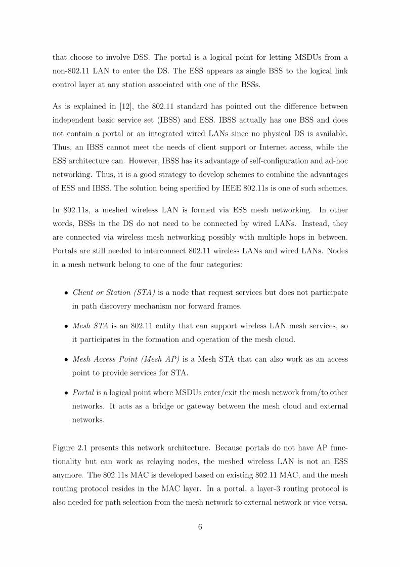
Figure 2.1 presents this network architecture. Because portals do not have AP func-
tionality but can work as relaying nodes, the meshed wireless LAN is not an ESS
anymore. The 802.11s MAC is developed based on existing 802.11 MAC, and the mesh
routing protocol resides in the MAC layer. In a portal, a layer-3 routing protocol is
also needed for path selection from the mesh network to external network or vice versa.
6
Figure 2.1: The 802.11s network architecture
2.2 Mesh formation and management
2.2.1 Mesh Profile
As is specified in the draft, there are three elements that characterize a mesh network:
• The Mesh ID
• The path selection protocol
• The path selection metric
Together these three elements define a profile. A Mesh STA can support different
profiles, but all nodes in a mesh cloud must share the same profile.
In infrastructured wireless networks, a Service Set Identifier (SSID) is used to dis-
tinguish the set of access points, which maintain a certain functional correlation and
belong to the same local area network. In a mesh network the same need for an iden-
tity exists, but instead of overloading the definition and function of the SSID, the draft
proposes a Mesh identifier or Mesh ID. Similarly to 802.11, beacon frames are used to
announce a Mesh ID and to avoid misleading a non-mesh station, Mesh STAs broadcast
beacons with the SSID set to a wildcard value.
IEEE 802.11s mandatory profile defines the Hybrid Wireless Mesh Protocol (HWMP)
as the path discovery mechanism and the Airtime Link Metric (ALM) as the path
7
selection metric (these are explained in the next section). The draft does not prevent
other protocols or metrics from being used in a mesh cloud, but it advises that a
mesh network shall not use more than one profile at the same time in order to avoid
complexity of profile renegotiation (that may be too expensive for a simple device to
handle).
2.2.2 Mesh creation
A mesh network is formed as Mesh STAs find neighbors that share the same profile.
The neighbor discovery mechanism is similar to what is currently proposed by the
IEEE 802.11 standard: active scanning (probe frame transmission) or passive scanning
(observation of beacon frames). In order to achieve this, every mesh station periodically
sends small one-hop management frames known as beacons.
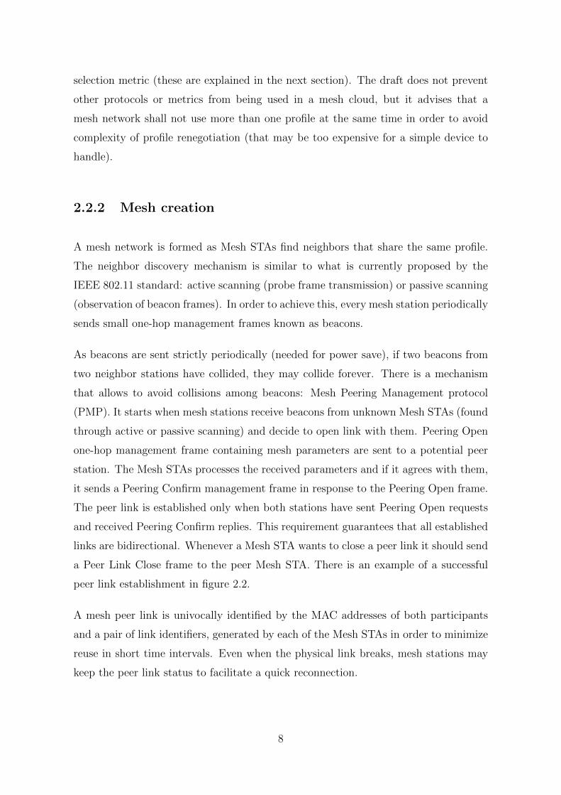
As beacons are sent strictly periodically (needed for power save), if two beacons from
two neighbor stations have collided, they may collide forever. There is a mechanism
that allows to avoid collisions among beacons: Mesh Peering Management protocol
(PMP). It starts when mesh stations receive beacons from unknown Mesh STAs (found
through active or passive scanning) and decide to open link with them. Peering Open
one-hop management frame containing mesh parameters are sent to a potential peer
station. The Mesh STAs processes the received parameters and if it agrees with them,
it sends a Peering Confirm management frame in response to the Peering Open frame.
The peer link is established only when both stations have sent Peering Open requests
and received Peering Confirm replies. This requirement guarantees that all established
links are bidirectional. Whenever a Mesh STA wants to close a peer link it should send
a Peer Link Close frame to the peer Mesh STA. There is an example of a successful
peer link establishment in figure 2.2.
A mesh peer link is univocally identified by the MAC addresses of both participants
and a pair of link identifiers, generated by each of the Mesh STAs in order to minimize
reuse in short time intervals. Even when the physical link breaks, mesh stations may
keep the peer link status to facilitate a quick reconnection.
8
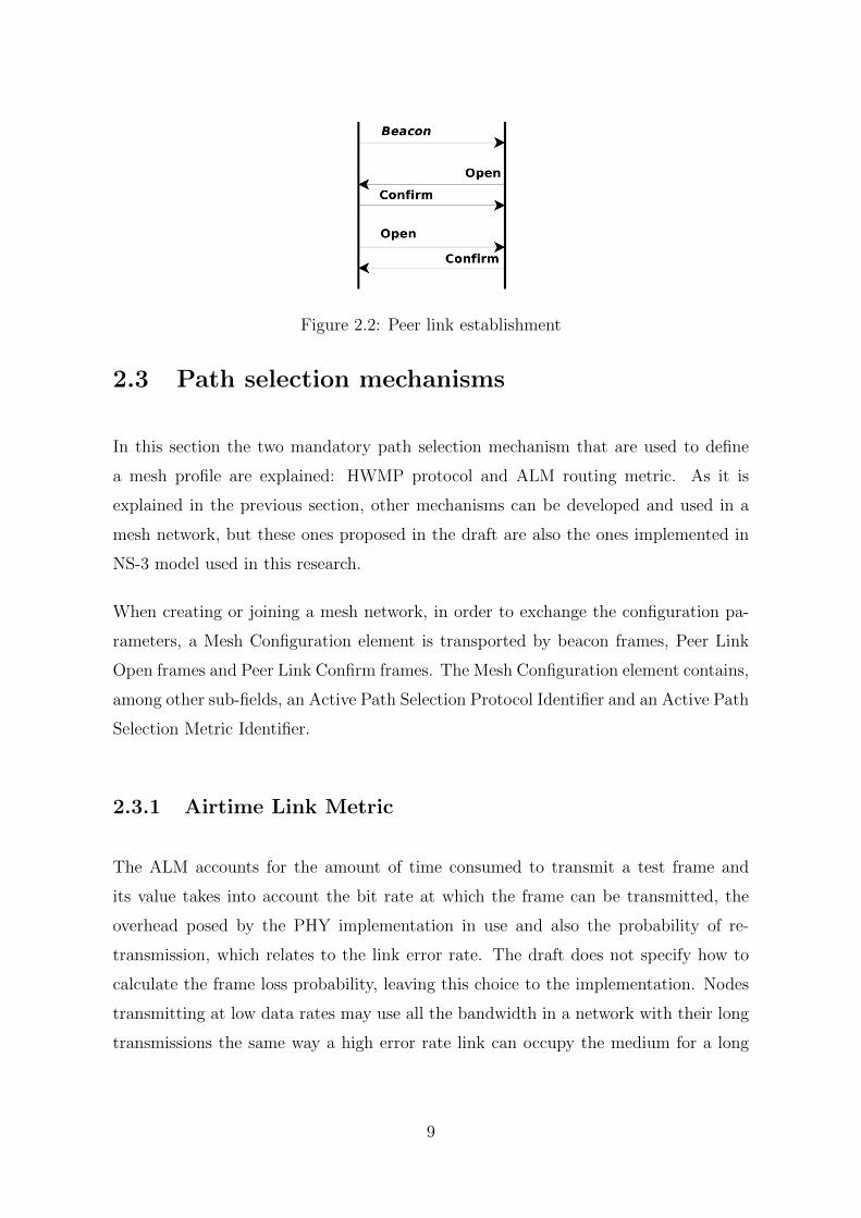
Figure 2.2: Peer link establishment
2.3 Path selection mechanisms
In this section the two mandatory path selection mechanism that are used to define
a mesh profile are explained: HWMP protocol and ALM routing metric. As it is
explained in the previous section, other mechanisms can be developed and used in a
mesh network, but these ones proposed in the draft are also the ones implemented in
NS-3 model used in this research.
When creating or joining a mesh network, in order to exchange the configuration pa-
rameters, a Mesh Configuration element is transported by beacon frames, Peer Link
Open frames and Peer Link Confirm frames. The Mesh Configuration element contains,
among other sub-fields, an Active Path Selection Protocol Identifier and an Active Path
Selection Metric Identifier.
2.3.1 Airtime Link Metric
The ALM accounts for the amount of time consumed to transmit a test frame and
its value takes into account the bit rate at which the frame can be transmitted, the
overhead posed by the PHY implementation in use and also the probability of re-
transmission, which relates to the link error rate. The draft does not specify how to
calculate the frame loss probability, leaving this choice to the implementation. Nodes
transmitting at low data rates may use all the bandwidth in a network with their long
transmissions the same way a high error rate link can occupy the medium for a long
9
time. The ALM is designed to avoid both problematics and according to the standard
the airtime cost, Ca, is calculated as:
Ca =
[OcaOp+
Bt
r
]1
1 − ef(2.1)
Where Oca is the channel access overhead and Op the protocol overhead which varies
according to the PHY layer implementation. Bt is the test frame size, r is the data rate
in Mbps at which the Mesh STA would transmit a test frame and ef is the measured
test frame error rate. Table 2.1 present the value for the constants Oca, Op and Bt for
each type of 802.11. During path discovery, each node in the path contributes to the
metric calculation by using management frames for exchanging routing information.
Table 2.1: ALM constants
Parameter 802.11a 802.11b Description
Oca 75µs 335µs Channel access overhead
Op 110µs 364µs Protocol overhead
Bt 8224 8224 # bits in test frame
2.3.2 Hybrid Wireless Mesh Protocol
The network infrastructure of 802.11 WMNs tends to have minimal mobility and most
of the traffic is to/from the Internet. However, some nodes such as handset devices,
laptops, etc. can be an Mesh STAs but definitely need mobility support. In order
to meet diverse requirements by making the routing protocol be efficient for different
scenarios, the Hybrid Wireless Mesh Protocol is being specified in 802.11s. In HWMP,
on-demand routing protocol is adopted for mesh nodes that experience a changing
environment, while proactive tree-based routing protocol is an efficient choice for mesh
nodes in a fixed network topology.
The on-demand routing protocol is specified based on Ad-hoc On-demand Distance
Vector (AODV) routing. Its basic features are adopted, but extensions are made for
802.11s. For more information on AODV check appendix A or the RFC of the IETF [1].
10
The proactive tree-based routing is applied when a root node is configured in the mesh
network. By means of the root, a distance vector tree can be built and maintained for
other nodes, which can avoid unnecessary routing overhead for routing path discovery
and recovery. On-demand routing and tree-based routing can run simultaneously.
The extensible framework of this protocol also supports other types of metrics apart
from the ALM (such as QoS parameters, traffic load, power consumption, etc.), but in
the same mesh only one metric shall be used.
Four information elements are specified for HWMP:
• Root announcement (RANN)
• Path request (PREQ)
• Path reply (PREP)
• Path error (PERR)
Except for PERR, all other information elements of HWMP contain three important
fields: destination sequence number (DSN), time-to-live (TTL), and metric. DSN and
TTL can prevent the counting to infinity problem, and the metric field helps to find a
better routing path than just using hop count.
On-demand routing mode
In the on-demand routing mode, an PREQ is broadcast by a source Mesh STA aiming
to set up a path to a destination Mesh STA. When an intermediate Mesh STA receives
this element, it creates/updates a path to the source if the sequence number of the
PREQ is greater than the previous one or the sequence number is the same but the
metric is better. If the intermediate Mesh STA has no path to the destination, it just
forwards the PREQ element further. Otherwise, there are different cases depending on
two flags, destination-only (DO) flag and reply-and-forward (RF) flag:
11
- [DO = 1] This is the default case. The intermediate Mesh STA does nothing but
just forwards the PREQ to the next-hop Mesh STA until the destination Mesh
STA. Once the destination gets this element, it sends a unicast PREP back to
the source. All intermediate Mesh STAs create a route to the destination when
receiving this PREP element. Thus, in this case the routing protocol just ignores
the existing route from the intermediate Mesh STA to the destination and creates
a new one. The RF flag has no effect on the routing protocol in this case.
- [DO = 0 and RF = 0] In this case, if the intermediate Mesh STA has a valid
route, it sends a unicast PREP to the source Mesh STA and does not forward
PREQ. Thus, the routing protocol uses the existing route from the intermediate
Mesh STA to the destination.
- [DO = 0 and RF = 1] In this case the intermediate Mesh STA sends a unicast
PREP to the source Mesh STA. Then, it needs to change the DO flag to 1 and
then forwards the PREQ element to the destination. By doing so, all the subse-
quent intermediate Mesh STAs will not send PREP elements to the source.
In maintenance PREQ, the DO flag is always set to 1 (first case). The third case exists
only when the source Mesh STA has no valid route and also wants to create a new
route to the destination Mesh STA. These procedures are specifically for HWMP and
different from the original AODV. An on-demand route discovery cicle is illustrated in
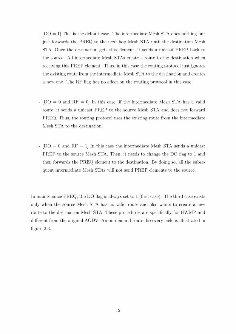
figure 2.3.
12
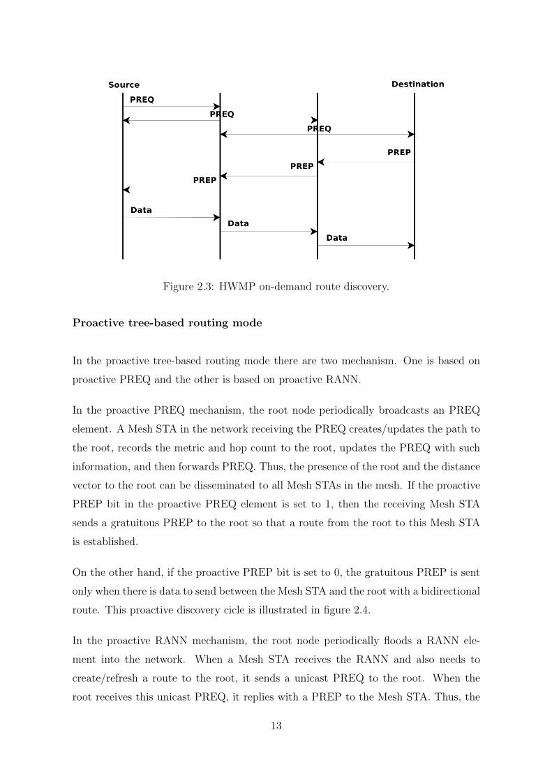
Figure 2.3: HWMP on-demand route discovery.
Proactive tree-based routing mode
In the proactive tree-based routing mode there are two mechanism. One is based on
proactive PREQ and the other is based on proactive RANN.
In the proactive PREQ mechanism, the root node periodically broadcasts an PREQ
element. A Mesh STA in the network receiving the PREQ creates/updates the path to
the root, records the metric and hop count to the root, updates the PREQ with such
information, and then forwards PREQ. Thus, the presence of the root and the distance
vector to the root can be disseminated to all Mesh STAs in the mesh. If the proactive
PREP bit in the proactive PREQ element is set to 1, then the receiving Mesh STA
sends a gratuitous PREP to the root so that a route from the root to this Mesh STA
is established.
On the other hand, if the proactive PREP bit is set to 0, the gratuitous PREP is sent
only when there is data to send between the Mesh STA and the root with a bidirectional
route. This proactive discovery cicle is illustrated in figure 2.4.
In the proactive RANN mechanism, the root node periodically floods a RANN ele-
ment into the network. When a Mesh STA receives the RANN and also needs to
create/refresh a route to the root, it sends a unicast PREQ to the root. When the
root receives this unicast PREQ, it replies with a PREP to the Mesh STA. Thus, the
13
Figure 2.4: HWMP proactive PREQ route discovery.
unicast PREQ forms the reverse route from the root to the originating Mesh STA,
while the unicast PREP creates the forward route from the originating Mesh STA to
the root.
2.4 Medium Access Control
Regarding the access to the medium, Mesh STAs implement the mesh coordination
function (MCF). As is described in [13], MCF consists of a mandatory and an optional
scheme. For the mandatory part, MCF relies on the contention-based protocol known
as Enhanced Distributed Channel Access (EDCA), which itself is an improved variant
of the basic 802.11 distributed coordination function (DCF). Using DCF, a station
transmits a single frame of arbitrary length.
Using EDCA, a station may transmit multiple frames whose total transmission du-
ration may not exceed the transmission opportunity (TXOP) limit. The intended
receiver acknowledges any successful frame reception. Additionally, EDCA differenti-
ates four traffic categories with different priorities in medium access and thereby allows
for limited support of quality of service (QoS).
To enhance QoS, MCF describes an optional medium access protocol called Mesh
Coordinated Channel Access (MCCA). It is a distributed reservation protocol that
14
allows Mesh STAs to avoid frame collisions. With MCCA, Mesh STAs reserve TXOPs
in the future called MCCA opportunities (MCCAOPs). An MCCAOP has a precise
start time and duration measured in slots of 32 µs. To negotiate an MCCAOP, a
Mesh STAs sends an MCCA setup request message to the intended receiver. Once
established, it advertise the MCCAOP via the beacon frames.
Since Mesh STAs outside the beacon reception range could conflict with the existing
MCCAOPs, Mesh STAs also include their neighbors’ MCCAOP reservations in the
beacon frame. At the beginning of an MCCA reservation, Mesh STAs other than
the MCCAOP owner refrain from channel access. The owner uses standard EDCA
to access the medium, and does not have priority over stations that do not support
MCCA.
Although this compromises efficiency, simulations (for example in [14]) reveal that
high medium utilization can still be achieved with MCCA in the presence of non-
MCCA devices. After an MCCA transmission ends, Mesh STAs use EDCA for medium
contention again.
2.5 Frame structure and syntax
In order to allow multihop functions at the MAC layer, the IEEE 802.11s emerging
standard extends the original 802.11 frame format and syntax. As is explained in [15],
the new frame format supports four or six MAC addresses and new frame subtypes are
introduced. The first two octets of an 802.11 frame contain the Frame Control field
and the third and fourth bits of this field identify the frame type, as shown in table
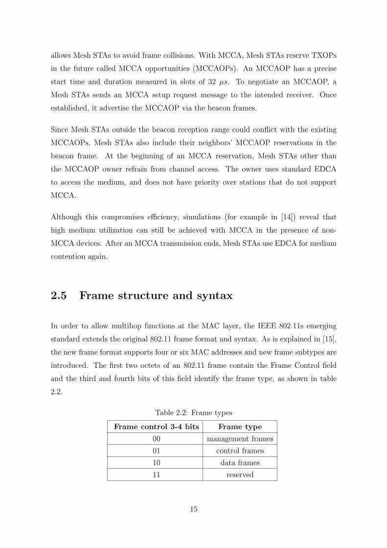
2.2.
Table 2.2: Frame types
Frame control 3-4 bits Frame type
00 management frames
01 control frames
10 data frames
11 reserved
15
Besides those two bits, there are also four more bits devoted to a frame subtype. Since
IEEE 802.11s is an amendment to IEEE 802.11, the frames it introduces must fall into
the four pre-existing categories. It was decided to extend the data and management
frames in the following ways:
• Data exchanged between Mesh STAs are transported by Mesh Data frames, de-
fined as data frames (type 0x2). where a mesh header is included in the frame
body.
• Mesh-specific management frames, such as PREP or PREQ, belong to type 0x0
(management) and subtype 0xD (action frames). There is also a new subtype
called Multihop Action frame. This new subtype refers to action frames with
four MAC addresses.
Another characteristic of the new frames is the use of the FromDS and ToDS flags. In
IEEE 802.11, those bits mark frames as being originated from or destined to a distribu-
tion system, which is the infrastructure that interconnects access points. Similarly to
a WDS, IEEE 802.11s also sets FromDS and ToDS flags in frames transmitted inside a
mesh cloud. Notice that both flags (FromDS and ToDS) are set to zero in ad-hoc IEEE
802.11 frames. In an ad-hoc network, peer- to-peer transfers can happen opportunis-
tically in a way that should not be confused with that proposed by a mesh network,
where frame forwarding (multihop forwarding) capabilities are present.
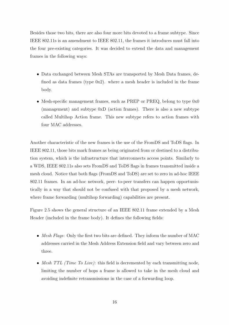
Figure 2.5 shows the general structure of an IEEE 802.11 frame extended by a Mesh
Header (included in the frame body). It defines the following fields:
• Mesh Flags : Only the first two bits are defined. They inform the number of MAC
addresses carried in the Mesh Address Extension field and vary between zero and
three.
• Mesh TTL (Time To Live): this field is decremented by each transmitting node,
limiting the number of hops a frame is allowed to take in the mesh cloud and
avoiding indefinite retransmissions in the case of a forwarding loop.
16
Figure 2.5: IEEE 802.11s frame structure
• Mesh Sequence Number : the three bytes of this field identify each frame and
allow duplicate detection, preventing unnecessary retransmissions inside the mesh
cloud.
• Mesh Address Extension: this field carries extra MAC addresses, since the mesh
network might need up to six addresses (below is explained in which cases this
may happen).
According to IEEE 802.11s, non-mesh nodes (STAs) can participate in the mesh
network through a Mesh STA with Access Point capabilities. STAs communicating
through the mesh cloud are proxied by their supporting Mesh APs and this scenario
constitutes one example where the six-address frame format is employed.
Four-address frames are originally supported by IEEE 802.11 for transmissions using a
WDS, but in order to support non-mesh stations, IEEE 802.11s frames need six MAC
addresses. The following are the six MAC addresses used, where the last two are the
additional ones needed.
1. SA (source address): the address of the node that generated the frame.
2. DA (destination address): the address of the node that is the final destination of
the frame.
3. TA (transmitter address): the address of the node that transmitted the frame.
It can be the same as the source address, or the address of any Mesh STA that
forwards the frame on behalf of the source (intermediate node)
17

4. RA (receiver address): the address of the node that receives the frame. It is the
address of the next-hop node and, on the last hop to the destination, it becomes
the same as DA.
5. Mesh SA: In a six-address frame, the SA is the source communication endpoint
(for example the node outside the mesh cloud that originates the frame). Then,
the Mesh SA is the node that introduces the frame in the mesh cloud (on behalf
of the SA).
6. Mesh DA: as the DA is defined as the final destination of the frame, the Mesh
DA is the address of the last node of the mesh cloud that handles the frame.
18
Chapter 3
IEEE 802.11s model in NS-3
This chapter provides an explanation of how is implemented the 802.11s wireless mesh
networking model in the Network Simulator 3 (NS-3) and which features or charac-
teristics are supported and which not. First, NS3 is briefly explained to see why this
simulator has been chosen.
The model used has been the one developed by the Wireless Software R&D Group of
IITP RAS and included in NS-3 from the release 3.6. Although it is based in the IEEE
P802.11s/D3.0 [16], for the aim of this research, the characteristics used and analyzed
are not different from the ones present in the last draft of 802.11s [3]. For more detailed
information, you can find the complete explanation in [17].
3.1 Network Simulator 3
NS-3 [18] is a discrete-event network simulator for Internet systems, targeted primarily
for research and educational use. NS-3 is free software, licensed under the GNU GPLv2
license, and is publicly available for research, development, and use.
It is a tool aligned with the simulation needs of modern networking research allowing
researchers to study Internet protocols and large-scale systems in a controlled environ-
ment. The following trends is how Internet research is being conducted are responded
by NS-3:
19
1. Extensible software core: written in C++ with optional Python interface and an
extensively documented API (doxygen [19]).
2. Attention to realism: model nodes more like a real computer and support key
interfaces such as sockets API and IP/device driver interface (in Linux).
3. Software integration: conforms to standard input/output formats (pcap trace
output, NS-2 mobility scripts, etc.) and adds support for running implementation
code.
4. Support for virtualization and testbeds : Develops two modes of integration with
real systems: 1) virtual machines run on top of ns-3 devices and channels, 2)
NS-3 stacks run in emulation mode and emit/consume packets over real devices.
5. Flexible tracing and statistics : decouples trace sources from trace sinks so we
have customizable trace sinks.
6. Attribute system: controls all simulation parameters for static objects, so you can
dump and read them all in configuration files.
7. New models : includes a mix of new and ported models.
To sump up, NS-3 tries to avoid some problems of its predecessor, NS-2, which is still
being used by many researchers, but it has some important lacks such as: interoper-
ability and coupling between models, lack of memory management, debugging of split
language objects or lack of realism (in the creation of packets for example).
Mainly, the new available high fidelity IEEE 802.11 MAC and PHY models together
with real world design philosophy and concepts made NS-3 the choice for developing
this 802.11s model as well as for carrying out this research.
20
3.2 Model design
To meet these requirements imposed by 802.11s of supporting multiple interfaces (wire-
less devices) and also different mesh networking protocol stacks, WS R&D Group
designed and implemented a runtime configurable multi-interface and multi-protocol
Mesh STA architecture.
In the next subsections, the supported and unsupported features are presented accord-
ing to the description of the draft presented in chapter 2.
3.2.1 Supported features
The most important features supported are the implementation of the Peering Man-
agement Protocol, the HWMP and the ALM.
A part from the functionality described in section2.3, the PMP includes link close
heuristics and beacon collision avoidance. HWMP includes proactive and on-demand
modes, unicast/broadcast propagation of management traffic and, as an extra function-
ality not specified yet in the draft, multi-radio extensions. However, for the moment
RANN mechanism is implemented but there is no support, so only the PREQ can be
used.
3.2.2 Unsupported features
The most important feature not implemented is Mesh Coordinated Channel Access
(MCCA) described in section 2.4. Internetworking using a Mesh Acces Point or a
Portal is not implemented neither, but this functionality is not needed to evaluate the
performance in the creation of mesh networks.
As other less relevant features not implemented we can point out the security, power
safe mode and although multi-radio operation is supported, no channel assignment
protocol is proposed.
21
3.3 Model implementation
The description of which modules are implemented in C++ and how they intercon-
nect with each other is presented in appendix B. The explanation is in a high-level in
order to see which modules and classes need to be accessed or created when designing
a mesh network, but the low-level code structure is not described. For more infor-
mation on each module and a more detailed low level explanation, please check NS-3
documentation under Doxygen [19].
First is explained the way the MAC-layer routing is implemented presenting the most
important classes. Then are analyzed the class MeshHelper (used to create a 802.11s
network easier) and MeshPointDevice (developed to create mesh point devices). They
provide some functions to configure the different parameters of the network and its
devices, so the main parameters and the way to configure them is studied.
Finally the parameters of the protocols HWMP and PMP are listed to see how can
they be configured according to their description in section 2.3.
3.4 MAC-layer routing model
The main part of the MAC-layer routing model is the specific type of a network
device, class MeshPointDevice. Being an interface to upper-layer protocols, it pro-
vides routing functionality hidden from upper-layer protocols, by means of the class
MeshL2RoutingProtocol.
This model supports stations with multiple network devices handled by a single MAC-
layer routing protocol. MeshPointDevice serves as an umbrella to multiple network
devices (”interfaces”) working under the same MAC-layer routing protocol. Network
devices may be of different types, each with a specific medium access method.
MAC-layer routing can be seen as a two-level model. MeshL2RoutingProtocol and
MeshPointDevice belong to the upper level. The task of MeshPointDevice is to send,
receive, and forward frames, while the task of MeshL2RoutingProtocol is to resolve
22
routes and keep frames waiting for route resolution. This functionality is independent
from the types of underlying network devices (”interfaces”).
The lower level implements the part of MAC-layer routing, specific for underlying
network devices and their medium access control methods. For example, HWMP
routing protocol in IEEE802.11s uses its own specific management frames.
This level is implemented as two base classes: MeshWifiInterfaceMac and MeshWifiIn-
terfaceMacPlugin. If beacon generation is enabled or disabled, it implements IEEE802.11s
mesh functionality or a simple ad-hoc functionality of the MAC-high part of the WiFi
model.
At present, HWMP with Peer management protocol (which is required by HWMP to
manage peer links) is implemented in this module.
23

Chapter 4
Simulations
4.1 Considerations
Before performing a simulation, four different aspects were considered to establish them
randomly:
• Node position
• Node sender and receiver
• Connection arrival distribution
• Duration of each connection
In ns-3 a global seed can be selected and also which run of this seed to use in the
simulations. Thus, when different protocols or variants of one are compared, it ensures
that the comparison is fair since they use exactly the same values of the four points
stated before.
There is no guarantee that the streams produced by two random seeds will not over-
lap using the ns-3 random generator. The only way to guarantee that two streams
do not overlap is to use the substream capability provided. Therefore, is better to
produce multiple independent runs of the same simulation so we guarantee there is no
25
correlations between them. If we set one seed, then it allows as to generate 2.3 × 10¹⁵
independent replications, more than enough if we consider that we usually use around
20 for each scenario.
Furthermore, according to [20], UDP constant bit rate (CBR) traffic must be used
to compare accurately since TCP has a slow start mechanism that can influence the
overall results.
4.2 Figures of merit
For all the protocols tested, the figures of merit taken into account are the followings:
• Average throughput: number of bits received divided by the difference between
the arrival time of the first packet and the last one.
• Average Packet Delivery Fraction (PDF): number of packets received divided by
the number of packets transmitted.
• Average end-to-end delay: the sum of the delay of all received packets divided
by the number of received packets.
• Average routing load ratio: the number of routing bytes received divided by the
number of data bytes received. A value of 1 means that the same amount of
routing bytes and data bytes has been transmitted.
To calculate some of the previous values, the implementation and advices given in [21]
have been used. When is needed, in some scenarios we also analyze the following figures
of merit:
• Number of peer links opened and closed.
• Number of routing packets generated: this concerns RREQ, RREP and RERR
packets.
26
4.3 Environment
The environment used in all the simulations is the one stated below. A log-distance
path loss propagation model has been used. Using this model we predict the loss a
signal encounters in densely populated areas over distance. Its parameters are:
Type: Log-distance path loss
Reference Distance = 1 m
Exponent = 2.7
Reference Loss = 46.7 dB
In all different tests performed, the devices present the following characteristics:
CCA Threshold = -62 dBm
Energy detection Threshold = -89 dBm
Transmission and Reception Gain = 1 dB
Minimum and maximum available transmission level = 18 dbm
Reception Noise Figure = 7 dB
The Clear Channel Assessment (CCA) is a mechanism for determining whether the
medium is idle or not. The CCA includes carrier sensing and energy detection. The
Carrier Sense (CS) mechanism consists of a physical CS and a virtual CS. The physical
CS is provided by the PHY and is a straightforward measuring of the received signal
strength of a valid 802.11 symbol. If it is above a certain level the medium is considered
busy.
The virtual CS is provided by the MAC and referred to as the Network Allocation
Vector (NAV). The NAV works as an indicator for the station when the medium will
become idle the next time and is kept current through the session duration values
included in all frames. The NAV is updated each time a valid 802.11 frame is received
that is not addressed to the receiving station, provided that the duration value is
greater then the current NAV value.
By examining the NAV a station may avoid transmitting even when the physical CS
indicates an idle medium. The energy detection procedure attempts to determine if the
medium is busy by measuring the total energy a station receives, regardless of whether
27
it is a valid 802.11 signal or not. If the received energy is above a certain level the
medium is considered busy. The thresholds for the carrier sense and energy detection
used have been the ones predefined in the 802.11a physical layer (taken into account
that, in the definition of the energy detection threshold of NS-3, the noise figure in
reception has to be considered).
4.3.1 Transmission rate
As explained in the previous sections, the physical model of 802.11a is used. It divides
data up into a series of symbols for transmission (for example at 54 Mbps each symbol
encodes 216 bits). The OFDM encoding used by 802.11a adds six bits for encoding
purposes to the end of the frame and also some more bits are used for the new mesh
frame format (see 2.5). The packet size used is 1024 bytes, the MAC header and Frame
Check Sequence (FCS) are 40 bytes and the mesh header can be up to 24 bytes.
Furthermore, the CSMA/CA network contention protocol is used to listen to the net-
work in order to avoid collisions. In CSMA/CA, as soon as a node needs to send a
packet, it checks if the channel is clear (no other node is transmitting at the time).
If the channel is clear, then the packet is sent. If it is not clear, the node waits for a
randomly chosen period of time and then it checks again. This period of time is called
the backoff factor, and is counted down by a backoff counter. If the channel is clear
when the backoff counter reaches zero, the node transmits the packet otherwise, the
backoff factor is set again and the process is repeated.
Thereby, the data rate available will decrease considerably. With these characteristics
and using the different transmission rates, HWMP can achieve the data rates presented
in table 4.1.
Each date rate presents different modulation and FEC (forward error correction) rates
in order to gain in robustness or in bit rate. That is why, for example, at 54 Mbps each
symbol encodes 216 bits while in 6 Mbps it encodes only 24. Thus, each transmission
rate can achieve the distances presented in figure 4.1.
28
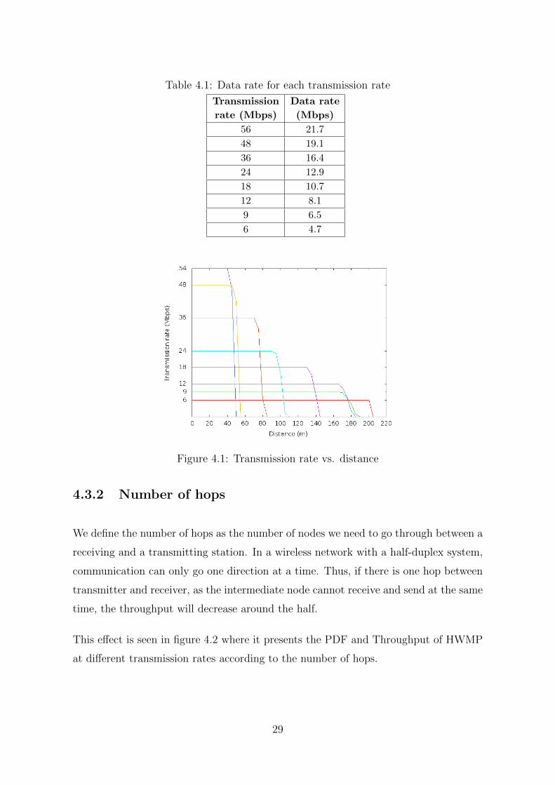
Table 4.1: Data rate for each transmission rate
Transmission Data rate
rate (Mbps) (Mbps)
56 21.7
48 19.1
36 16.4
24 12.9
18 10.7
12 8.1
9 6.5
6 4.7
Figure 4.1: Transmission rate vs. distance
4.3.2 Number of hops
We define the number of hops as the number of nodes we need to go through between a
receiving and a transmitting station. In a wireless network with a half-duplex system,
communication can only go one direction at a time. Thus, if there is one hop between
transmitter and receiver, as the intermediate node cannot receive and send at the same
time, the throughput will decrease around the half.
This effect is seen in figure 4.2 where it presents the PDF and Throughput of HWMP
at different transmission rates according to the number of hops.
29
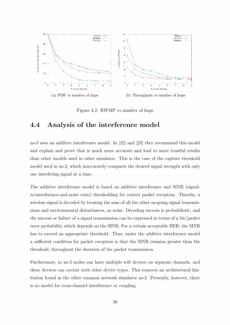
(a) PDF vs number of hops (b) Throughput vs number of hops
Figure 4.2: HWMP vs number of hops
4.4 Analysis of the interference model
ns-3 uses an additive interference model. In [22] and [23] they recommend this model
and explain and prove that is much more accurate and lead to more trustful results
than other models used in other simulator. This is the case of the capture threshold
model used in ns-2, which inaccurately compares the desired signal strength with only
one interfering signal at a time.
The additive interference model is based on additive interference and SINR (signal-
to-interference-and-noise ratio) thresholding for correct packet reception. Thereby, a
wireless signal is decoded by treating the sum of all the other on-going signal transmis-
sions and environmental disturbances, as noise. Decoding success is probabilistic, and
the success or failure of a signal transmission can be expressed in terms of a bit/packet
error probability which depends on the SINR. For a certain acceptable BER, the SINR
has to exceed an appropriate threshold. Thus, under the additive interference model
a sufficient condition for packet reception is that the SINR remains greater than the
threshold, throughout the duration of the packet transmission.
Furthermore, in ns-3 nodes can have multiple wifi devices on separate channels, and
these devices can coexist with other device types. This removes an architectural lim-
itation found in the other common network simulator ns-2. Presently, however, there
is no model for cross-channel interference or coupling.
30
Some scenarios have been analyzed to evaluate this interference model. In order to
see the effect clearer, the nodes always send packets close to the maximum data rate
available in the link (see table 4.1).
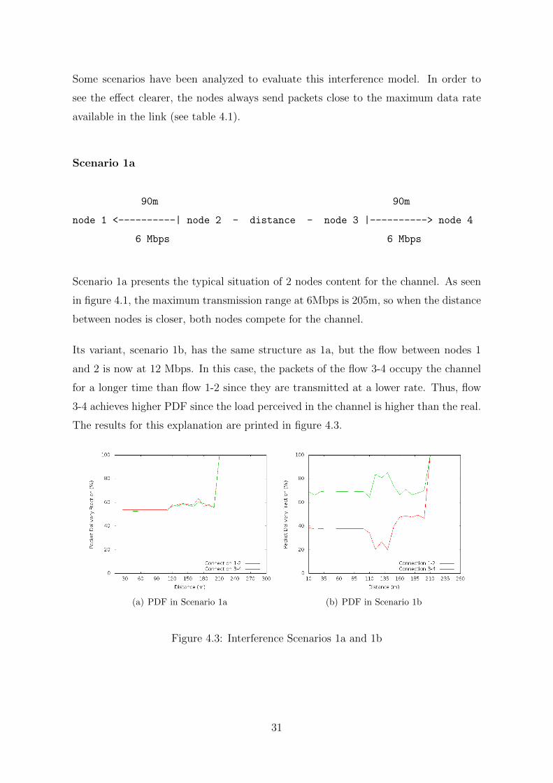
Scenario 1a
90m 90m
node 1 <----------| node 2 - distance - node 3 |----------> node 4
6 Mbps 6 Mbps
Scenario 1a presents the typical situation of 2 nodes content for the channel. As seen
in figure 4.1, the maximum transmission range at 6Mbps is 205m, so when the distance
between nodes is closer, both nodes compete for the channel.
Its variant, scenario 1b, has the same structure as 1a, but the flow between nodes 1
and 2 is now at 12 Mbps. In this case, the packets of the flow 3-4 occupy the channel
for a longer time than flow 1-2 since they are transmitted at a lower rate. Thus, flow
3-4 achieves higher PDF since the load perceived in the channel is higher than the real.
The results for this explanation are printed in figure 4.3.
(a) PDF in Scenario 1a (b) PDF in Scenario 1b
Figure 4.3: Interference Scenarios 1a and 1b
31
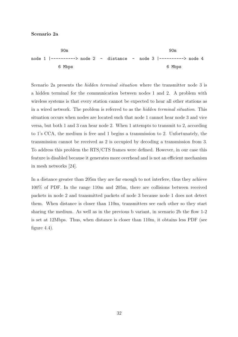
Scenario 2a
90m 90m
node 1 |----------> node 2 - distance - node 3 |----------> node 4
6 Mbps 6 Mbps
Scenario 2a presents the hidden terminal situation where the transmitter node 3 is
a hidden terminal for the communication between nodes 1 and 2. A problem with
wireless systems is that every station cannot be expected to hear all other stations as
in a wired network. The problem is referred to as the hidden terminal situation. This
situation occurs when nodes are located such that node 1 cannot hear node 3 and vice
versa, but both 1 and 3 can hear node 2. When 1 attempts to transmit to 2, according
to 1’s CCA, the medium is free and 1 begins a transmission to 2. Unfortunately, the
transmission cannot be received as 2 is occupied by decoding a transmission from 3.
To address this problem the RTS/CTS frames were defined. However, in our case this
feature is disabled because it generates more overhead and is not an efficient mechanism
in mesh networks [24].
In a distance greater than 205m they are far enough to not interfere, thus they achieve
100% of PDF. In the range 110m and 205m, there are collisions between received
packets in node 2 and transmitted packets of node 3 because node 1 does not detect
them. When distance is closer than 110m, transmitters see each other so they start
sharing the medium. As well as in the previous b variant, in scenario 2b the flow 1-2
is set at 12Mbps. Thus, when distance is closer than 110m, it obtains less PDF (see
figure 4.4).
32
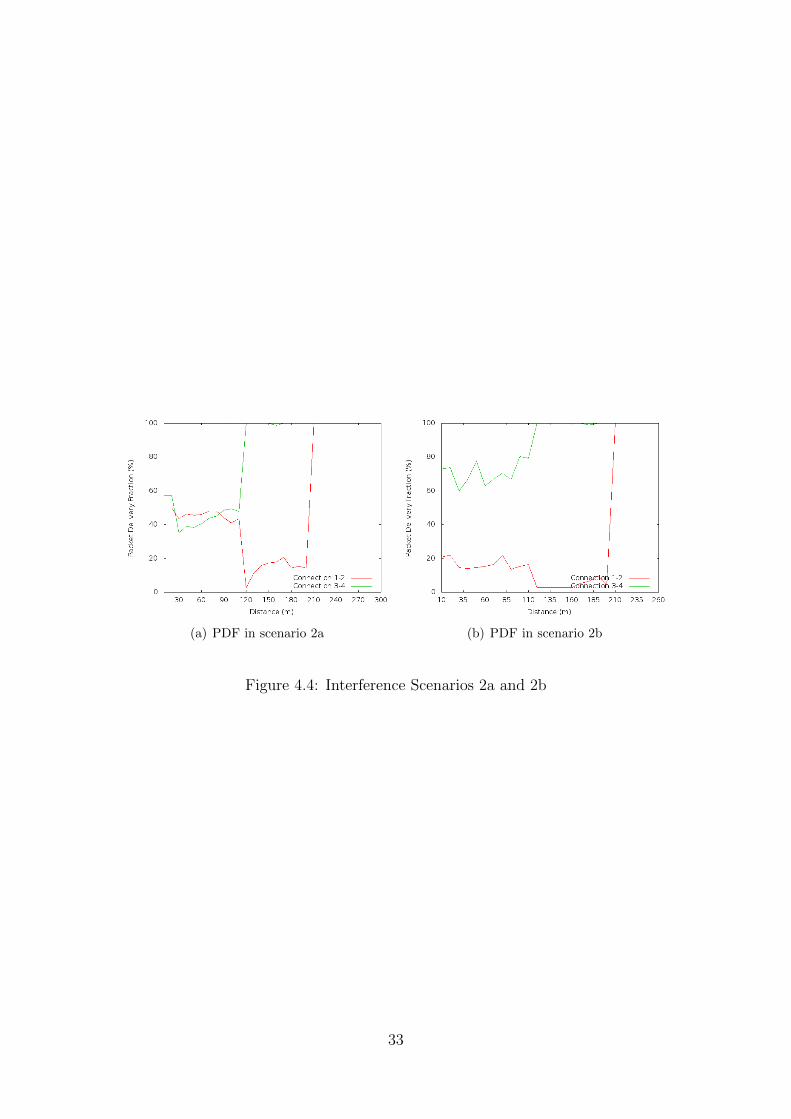
(a) PDF in scenario 2a (b) PDF in scenario 2b
Figure 4.4: Interference Scenarios 2a and 2b
33

Chapter 5
HWMP vs. AODV
HWMP is based in AODV but using layer 2 routing instead of layer 3 routing. Thus,
one question could be to know if this new layer 2 routing protocol proposed for mesh
networks will work better than the traditional layer 3 routing.
To answer this question these two protocols were configured to work under the same
conditions and we evaluated their performance in terms of scalability (nodes and con-
nections).
HWMP protocol implemented in this ns-3 version is explained in section 2.3.2 and
appendix B.3. In the appendix A you can find the explanation of the AODV version
on which the ns-3 implementation is based.
5.1 Configuration
First of all, AODV and HWMP had to be configured using the same values for their
parameters taking into account the differences they present. By doing this, we assure
the comparison is fair and the difference in their performances will be caused by their
own ways to route packets (and not because one allows more RREQ packets than the
other, for example).
35
After several tests, HWMP and AODV were configured as shown in table 5.1. In order
to compare accurately both protocols, some default values had to be changed. One
important point was to be sure to activate in both the destination only flag in order
to work as explained in 2.3.2.
The Beacon Collision Avoidance (BCA) mechanism of HWMP is used to detect and
mitigate collisions among beacon frames transmitted by other stations on the same
channel within the range of 2 hops. However, this system produces very limited ad-
vantages when no hidden stations are present and reduces the throughput. Thus, it
was disabled to not drop down the performance of HWMP.
Other important parameters which had to be changed were the Allowed Hello Loss in
AODV and the Max Beacon Loss in HWMP. Especially in the case of this last one, its
initial number was set to 2 (which is extremely low) and sometimes due to the prop-
agation model losses, some connection were set as not valid beforehand. The other
parameters changed were some packets thresholds and retries that can be checked in
the table 5.1.
5.2 Routing metric
One important aspect that must be taken into account is that HWMP uses a radio-
aware routing metric (the Airtime Link Metric, see 2.3.1). On the other hand, AODV
uses the simple hop count metric. So the comparison is being made between a layer
2 routing protocol with a radio-aware metric and a layer 3 routing protocol with hop
count metric.
With the following test, the importance of the routing metric can be observed. Usually
the transmission rate to send control information goes at 6Mbps (this is a broadcast
information, so the most robust modulation is used), while the data transmission can
use higher rates. Fixing the control rate at 6Mbps, the hop count metric will establish
some paths that higher rates of data packets will not be able to use. On the other
hand, while ALM is also affected, as it takes into account the frame error rate, it
selects better routes.
36
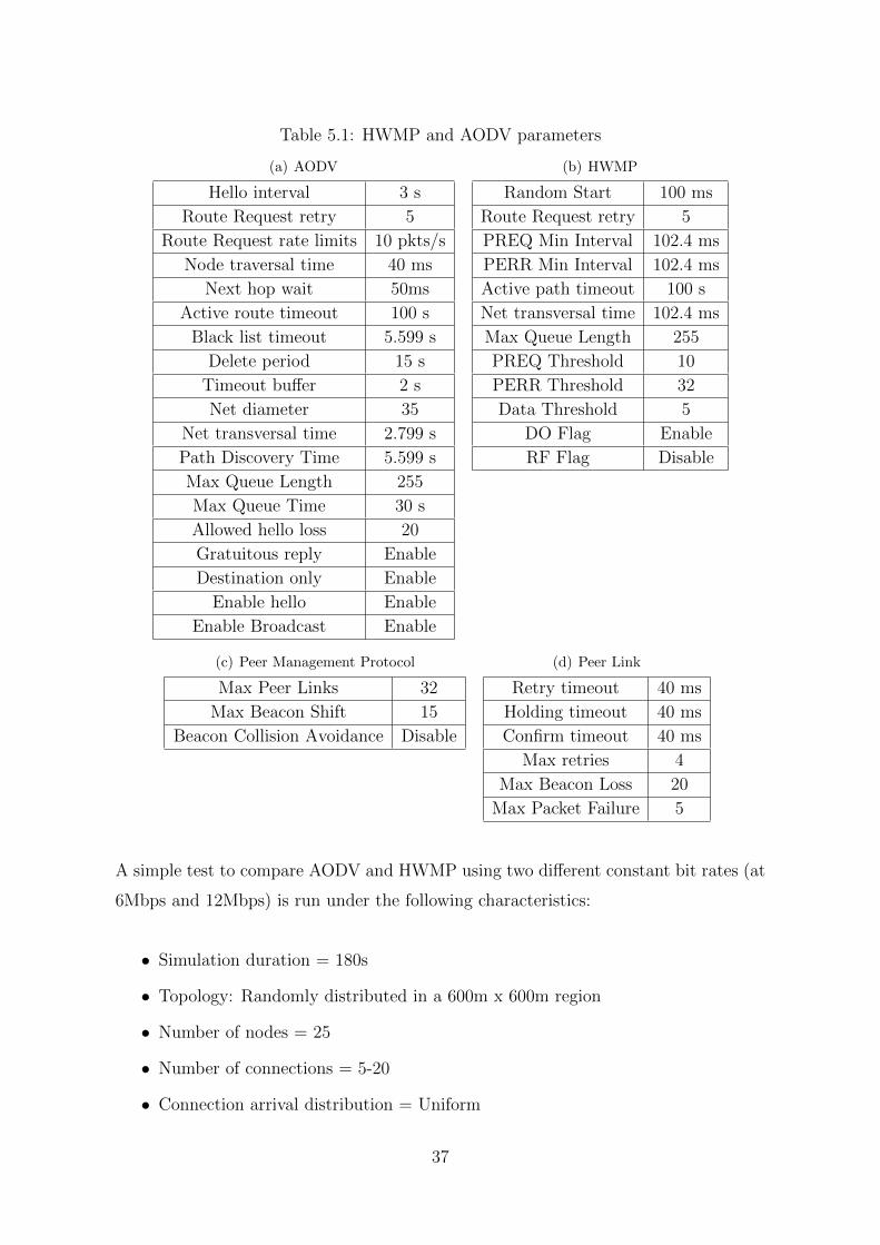
Table 5.1: HWMP and AODV parameters
(a) AODV
Hello interval 3 s
Route Request retry 5
Route Request rate limits 10 pkts/s
Node traversal time 40 ms
Next hop wait 50ms
Active route timeout 100 s
Black list timeout 5.599 s
Delete period 15 s
Timeout buffer 2 s
Net diameter 35
Net transversal time 2.799 s
Path Discovery Time 5.599 s
Max Queue Length 255
Max Queue Time 30 s
Allowed hello loss 20
Gratuitous reply Enable
Destination only Enable
Enable hello Enable
Enable Broadcast Enable
(b) HWMP
Random Start 100 ms
Route Request retry 5
PREQ Min Interval 102.4 ms
PERR Min Interval 102.4 ms
Active path timeout 100 s
Net transversal time 102.4 ms
Max Queue Length 255
PREQ Threshold 10
PERR Threshold 32
Data Threshold 5
DO Flag Enable
RF Flag Disable
(c) Peer Management Protocol
Max Peer Links 32
Max Beacon Shift 15
Beacon Collision Avoidance Disable
(d) Peer Link
Retry timeout 40 ms
Holding timeout 40 ms
Confirm timeout 40 ms
Max retries 4
Max Beacon Loss 20
Max Packet Failure 5
A simple test to compare AODV and HWMP using two different constant bit rates (at
6Mbps and 12Mbps) is run under the following characteristics:
• Simulation duration = 180s
• Topology: Randomly distributed in a 600m x 600m region
• Number of nodes = 25
• Number of connections = 5-20
• Connection arrival distribution = Uniform
37
• Duration of each connection = Exponential (mean = 25s)
• Data rate of each connection = 200 Kbps
• Packet size = 1024 bytes
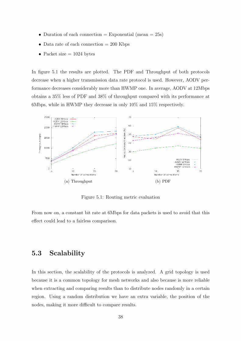
In figure 5.1 the results are plotted. The PDF and Throughput of both protocols
decrease when a higher transmission data rate protocol is used. However, AODV per-
formance decreases considerably more than HWMP one. In average, AODV at 12Mbps
obtains a 35% less of PDF and 38% of throughput compared with its performance at
6Mbps, while in HWMP they decrease in only 10% and 15% respectively.
(a) Throughput (b) PDF
Figure 5.1: Routing metric evaluation
From now on, a constant bit rate at 6Mbps for data packets is used to avoid that this
effect could lead to a fairless comparison.
5.3 Scalability
In this section, the scalability of the protocols is analyzed. A grid topology is used
because it is a common topology for mesh networks and also because is more reliable
when extracting and comparing results than to distribute nodes randomly in a certain
region. Using a random distribution we have an extra variable, the position of the
nodes, making it more difficult to compare results.
38
The grid topologies evaluated are 3x3 (9 nodes), 4x4 (16 nodes), 5x5 (25 nodes) and
6x6 (36 nodes) with 170 meters of separation between nodes. This guarantees that
nodes can only reach directly the closed neighbors and they need to look for a paths
to reach the rest (see results in 4.3.1).
The number of random connections established between the nodes of the scenario is
the same as the number of nodes. They present a uniform arrival distribution with a
duration generated by an exponential variable with a mean of 30 seconds. Using these
parameters we can be sure that with a 300 seconds simulation several connections will
overlap.
The packet size is set to 1024 bytes and the parameter swept is the data rate of each
connection. They start at 50 Kbps until 400 Kbps, so at certain point the network will
be loaded enough to see how each protocol deals with congestion.
5.3.1 Results
As it was explained in 5.2, a different metric can be the reason for important differences.
To be able to see what causes the difference between HWMP and AODV performance,
a third protocol has been tested: HWMP using hop count metric instead of ALM. The
complete results for the figures of merit discussed below are placed at the end of this
chapter in figures 5.5, 5.6, 5.7 and 5.8.
PDF and Throughput
Checking the results for the several scenarios, in smaller grids, the PDF and throughput
are slightly better using HWMP, while in larger grids AODV performs the best. This
is because ALM obtains worse metric values when links are already being used or
interfered (higher error rates in the links) and it tries to find another free path to avoid
collisions (although this is not always the best option). This also explains that, when
selecting a high data rate in a small grid, HWMP is no longer better than AODV (for
example at 400kbps in 4x4). When there is congestion or high load, the error rates
increases due to collision and the metric gets worse.
39
Furthermore, in all cases HWMP hop count performance is between AODV and HWMP
which helps us prove that one of the main reasons of the difference in throughput and
PDF when increasing nodes and connections is the metric.
In average, HWMP outperforms AODV in a 3x3 and 4x4 grid while, in a 6x6 grid,
AODV is the best (in a 5x5 grid they present a similar performance). Thus, AODV
works better than HWMP in terms of PDF and throughput when the number of nodes
and connections are higher. However this difference means a 5% of PDF in the worse
case while usually is less than 3%. Depending on the requirement of the application
used, other figures of merit may present a more significant difference.
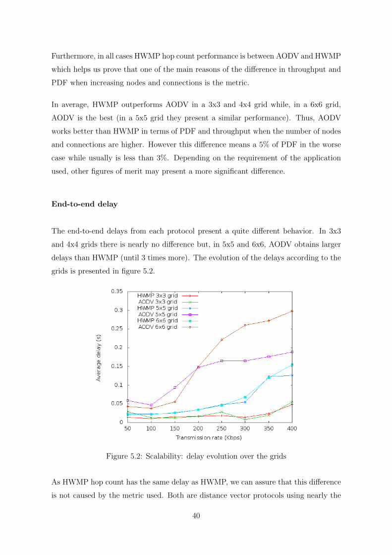
End-to-end delay
The end-to-end delays from each protocol present a quite different behavior. In 3x3
and 4x4 grids there is nearly no difference but, in 5x5 and 6x6, AODV obtains larger
delays than HWMP (until 3 times more). The evolution of the delays according to the
grids is presented in figure 5.2.
Figure 5.2: Scalability: delay evolution over the grids
As HWMP hop count has the same delay as HWMP, we can assure that this difference
is not caused by the metric used. Both are distance vector protocols using nearly the
40
same mechanism so a closer look is necessary to determine the reason. By checking the
flows in an scenario, we find out that this delay difference is caused when connections
like the ones presented in table 5.2 appear (flow extracted from a 5x5 grid scenario at
50kbps).
Table 5.2: Scalability: detailed results of a connection
Results AODV HWMP
PDF (%) 39.92 97.58
Average delay (s) 0.7912 0.0094
Rx bitrate (kbps) 33.91 48.87
Tx bitrate (kbps) 50.37 50.37
Time First Tx Packet (s) 68.783 68.783
Time First Rx Packet (s) 86.594 69.636
Time Last Tx Packet (s) 109.252 109.252
Time Last Rx Packet (s) 109.952 109.255
Delay Sum (s) 78.329 2.272
Last Delay (s) 0.7002 0.003
Tx Packets 248 248
Lost Packets 172 6
Time Forwarded 124 0
This example clearly shows that the delay difference is caused by the route discovery
mechanism. Since a node wants to send the first packet until it reaches the destination,
HWMP needs around 1 seconds while AODV needs 18. AODV sends a RREQ and after
a certain time without receiving a RREP it sends again a RREQ (until the maximum
number set, 5 in this case). Not all these packets are lost in collisions, but due to
congestion in some nodes, they are queued and delivered later.
In HWMP this does not happen because the layer 2 control packets have priority and
can cross a link even though this is saturated. This point could make think that
AODV should have less PDF than HWMP. As was explained before, with the airtime
link metric, HWMP tries to avoid links being used and in some occasions it choses a
too long path or even does not find a good route. This effect of the ALM compensates
the other from AODV and this is why the average PDF results are similar.
However, it must be pointed out that this compensation is not always present. The
metric problem of HWMP becomes worse when there are more connections and conges-
tion. Regarding the results using 350-400Kbps in all the scenarios, AODV and HWMP
41
hop count always perform better than standard HWMP using ALM.
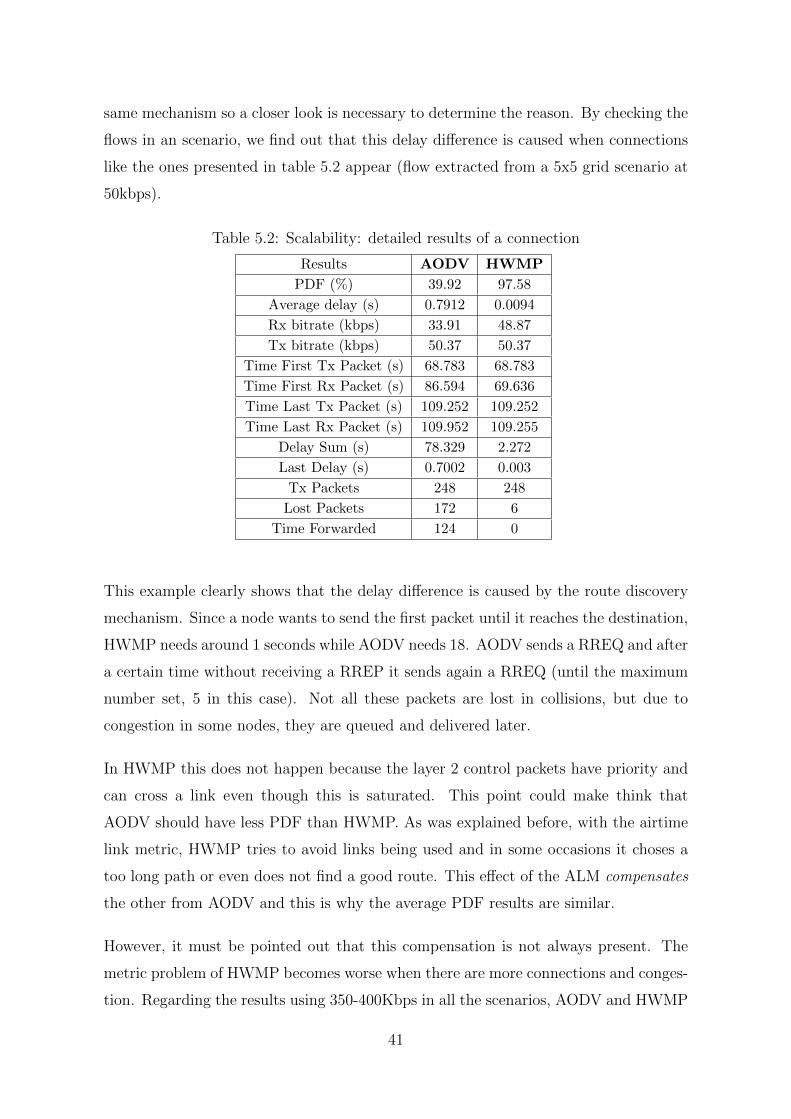
In figure 5.3 are plotted the delays of all the connections from the previous example.
Although HWMP routing is usually faster than the AODV one, the responsible for this
high delay difference are the few connections similar to the one in table 5.2. The flow
from the table is number 0 and, as well as flows 13, 20 and 23, the delay generated is
higher than 0.7 seconds. On the other hand, HWMP and AODV have 18 flows out of
25 with a delay smaller than 0.05 seconds and, as HWMP do not present flows with
such a higher delay, the average results are considerably smaller.
Figure 5.3: Scalability: detailed delay of a connection
In all cases we see that HWMP outperforms AODV in terms of delay in a significant
way. This figure of merit is really important in real time application and may be a
crucial aspect when deciding which protocol to use.
Routing Load Ratio
The routing load ratio also presents a significant difference although, depending on the
amount and type of traffic, it may not be as important as the previous one in terms
of QoS. First of all, remember that AODV uses a hello messages mechanism, while
HWMP does not need it. This hello mechanism is the one responsible for the main
42
part of routing load generated by AODV. Thus, since the hello interval is set at 3
seconds, AODV will always presents much more routing load ratio than HWMP.
As the routing load ratio is calculated dividing the routing load bytes received by the
data bytes received (as is explained in 4.2) if more and more data bytes are delivered
without the need of more routing information, the routing load ratio decreases. This
is what happen in the 3x3 grid scenario (figure 5.5). The bit rate of the connections
increases but the PDF does not decrease which means that more packets are delivered
with the same routing information. Thus, the routing load ratio decreases proportion-
ally to the increase of bit rate. Specifically, in AODV it goes from a 0.08 ratio until
0.01 (factor of 8) and in HWMP from 0.02 until 0.005 (factor of 4).
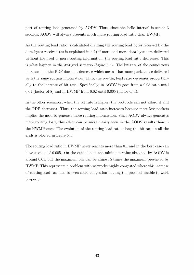
In the other scenarios, when the bit rate is higher, the protocols can not afford it and
the PDF decreases. Thus, the routing load ratio increases because more lost packets
implies the need to generate more routing information. Since AODV always generates
more routing load, this effect can be more clearly seen in the AODV results than in
the HWMP ones. The evolution of the routing load ratio along the bit rate in all the
grids is plotted in figure 5.4.
The routing load ratio in HWMP never reaches more than 0.1 and in the best case can
have a value of 0.005. On the other hand, the minimum value obtained by AODV is
around 0.01, but the maximum one can be almost 5 times the maximum presented by
HWMP. This represents a problem with networks highly congested where this increase
of routing load can deal to even more congestion making the protocol unable to work
properly.
43
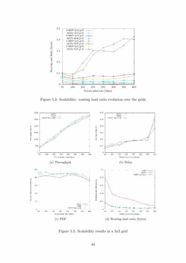
Figure 5.4: Scalability: routing load ratio evolution over the grids
(a) Throughput (b) Delay
(c) PDF (d) Routing load ratio (bytes)
Figure 5.5: Scalability results in a 3x3 grid
44
(a) Throughput (b) Delay
(c) PDF (d) Routing load ratio (bytes)
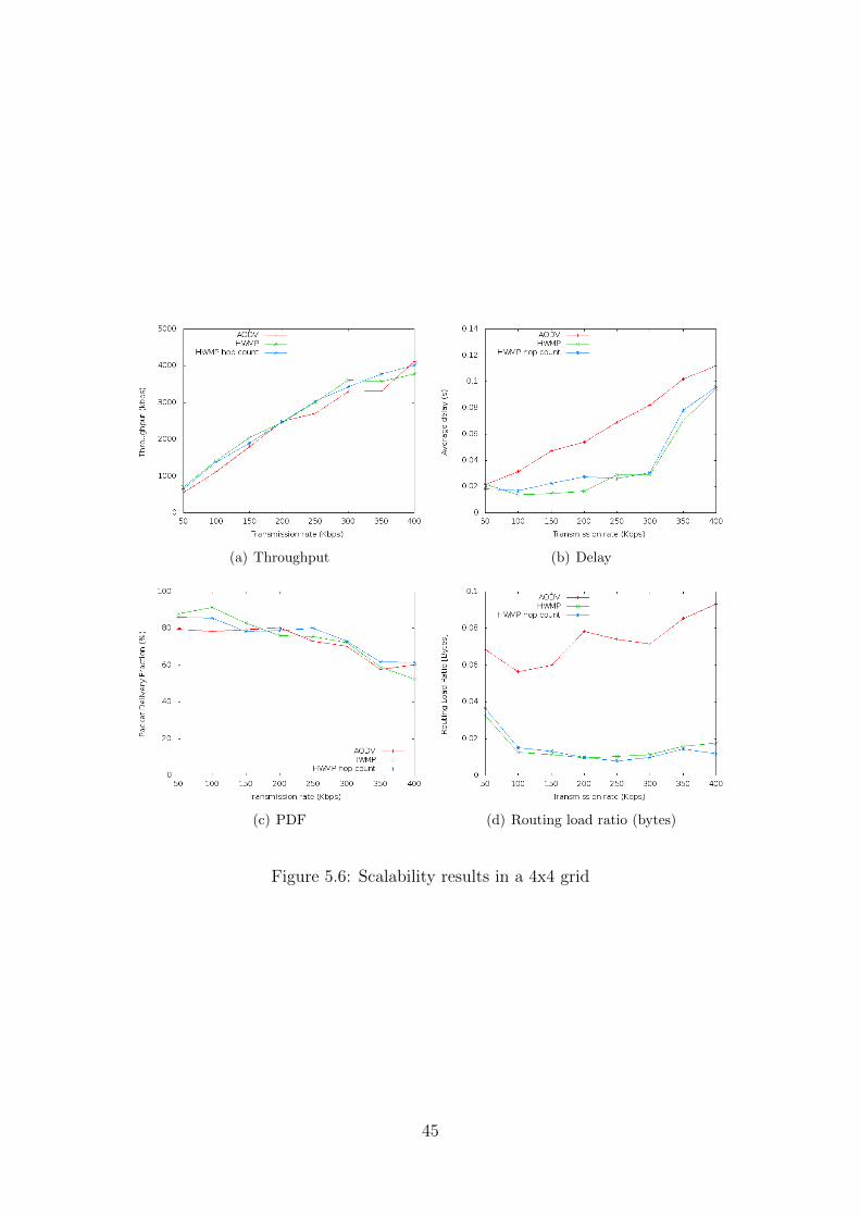
Figure 5.6: Scalability results in a 4x4 grid
45
(a) Throughput (b) Delay
(c) PDF (d) Routing load ratio (bytes)
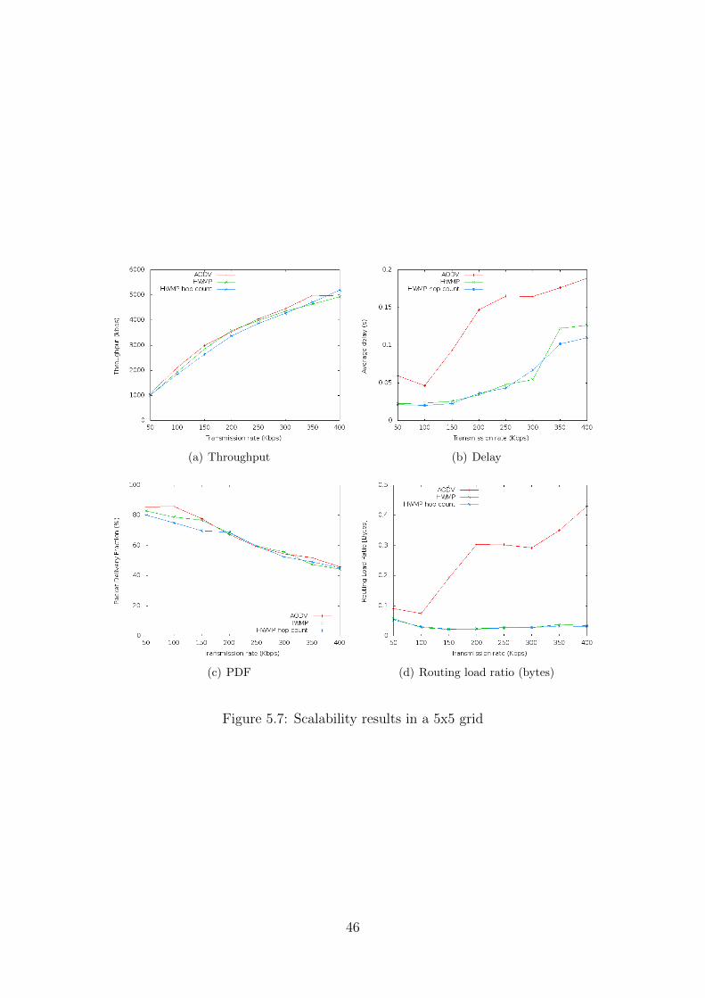
Figure 5.7: Scalability results in a 5x5 grid
46
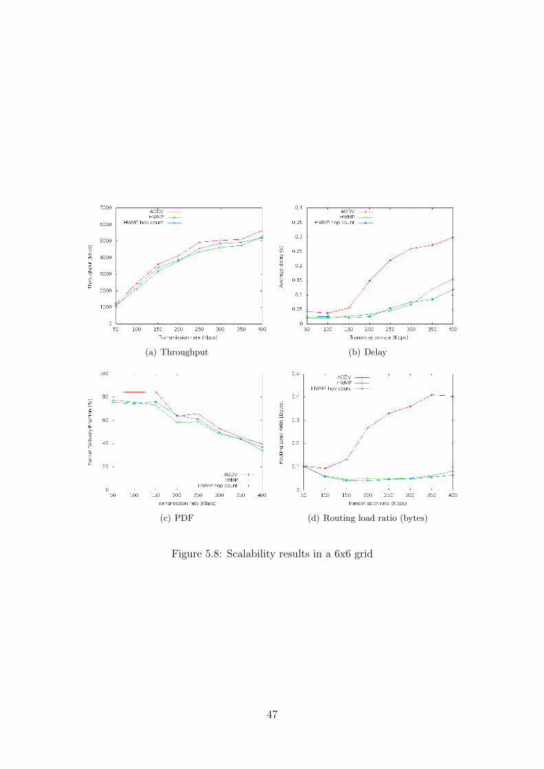
(a) Throughput (b) Delay
(c) PDF (d) Routing load ratio (bytes)
Figure 5.8: Scalability results in a 6x6 grid
47

Chapter 6
HWMP Reactive vs. Proactive
As is explained in 2.3.2, the Hybrid Wireless Mesh Protocol can work in a reactive and
in a proactive routing mode. When creating a 802.11s network, something useful to
know could be in which situations the reactive or the proactive mode should be used.
In this chapter the on-demand path selection mode (reactive) and the proactive tree
building mode using PREQ mechanism are analyzed.
The proactive mode ensures that all nodes have a path defined to the root at all time,
so if a node wants to send information to the root there is no need to start a route
discovery procedure. On the other hand, if a node wants to send information to another
node (which is not the root), the sender has to ask to its superior neighbor in the tree
structure if he knows how to reach the target. This action continues until some node
up in the tree knows the way. In the worst case, it will reach the root of the tree (the
root node) who knows a path to all nodes in the network.
This tree mechanism implies that if you want to reach a node member of another
branch of the tree, the chosen path will go through the root node. If the main part
of the traffic of the mesh network is between internal nodes, this mechanism seams
not so good because it generates longer paths and can create congestion in the root
node. However, if the main part of the traffic of the mesh network has an external
destination, this tree mechanism seems a good option because all nodes need to send
the information to the root (which is used as Portal) in order to reach the exterior.
49
To summarize, when there is internal traffic, the reactive mode seems a better option
while in the case of external traffic, the proactive mode should work better.
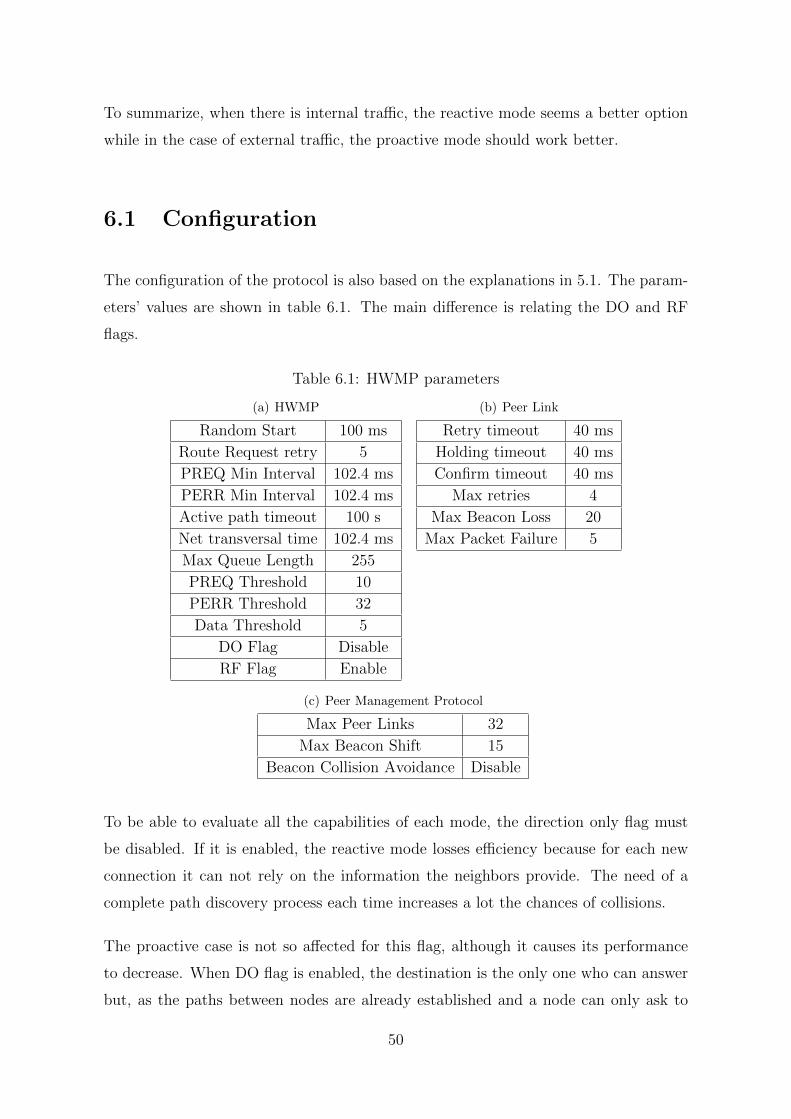
6.1 Configuration
The configuration of the protocol is also based on the explanations in 5.1. The param-
eters’ values are shown in table 6.1. The main difference is relating the DO and RF
flags.
Table 6.1: HWMP parameters
(a) HWMP
Random Start 100 ms
Route Request retry 5
PREQ Min Interval 102.4 ms
PERR Min Interval 102.4 ms
Active path timeout 100 s
Net transversal time 102.4 ms
Max Queue Length 255
PREQ Threshold 10
PERR Threshold 32
Data Threshold 5
DO Flag Disable
RF Flag Enable
(b) Peer Link
Retry timeout 40 ms
Holding timeout 40 ms
Confirm timeout 40 ms
Max retries 4
Max Beacon Loss 20
Max Packet Failure 5
(c) Peer Management Protocol
Max Peer Links 32
Max Beacon Shift 15
Beacon Collision Avoidance Disable
To be able to evaluate all the capabilities of each mode, the direction only flag must
be disabled. If it is enabled, the reactive mode losses efficiency because for each new
connection it can not rely on the information the neighbors provide. The need of a
complete path discovery process each time increases a lot the chances of collisions.
The proactive case is not so affected for this flag, although it causes its performance
to decrease. When DO flag is enabled, the destination is the only one who can answer
but, as the paths between nodes are already established and a node can only ask to
50
the upper branch of the tree, it does not interfere so much in the performance. The
proactive tree structure guarantees a routing order in the uses of paths that the reactive
mode does not provide.
6.2 Destination Only flag
To check the previous discussed effect of the destination only flag, the analysis of an
small rectangular scenario is proposed. In a small scenario where one node can reach
another one with usually one, two or maximum three hops, both protocols should have
a similar performance if the DO flag is disabled. However, with the DO flag enabled, by
forcing always a route discovery in the reactive mode, its performance should decrease.
As explained before, lots of collisions will appear and, in this case, the effect will be
worse because the node density is high. The scenario analyzed presents the following
parameters:
• Simulation duration = 180s
• Topology: Randomly distributed in a 450m x 150m region
• Number of nodes = 20
• Number of connections = 20
• Connection arrival distribution = Uniform
• Duration of each connection = Exponential (mean = 25s)
• Data rate of each connection = 150 Kbps
• Packet size = 1024 bytes
For each variant of the scenario, N connections are defined and the number of connec-
tion that have as destination the root node is increased. It starts by setting all nodes to
send information randomly to another node of the mesh network and each time more
and more nodes change their destination to the root node (so simulating they send
traffic to the exterior).
51
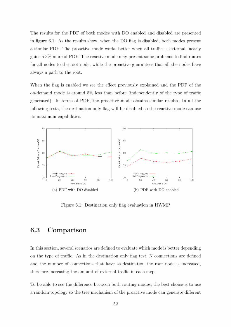
The results for the PDF of both modes with DO enabled and disabled are presented
in figure 6.1. As the results show, when the DO flag is disabled, both modes present
a similar PDF. The proactive mode works better when all traffic is external, nearly
gains a 3% more of PDF. The reactive mode may present some problems to find routes
for all nodes to the root node, while the proactive guarantees that all the nodes have
always a path to the root.
When the flag is enabled we see the effect previously explained and the PDF of the
on-demand mode is around 5% less than before (independently of the type of traffic
generated). In terms of PDF, the proactive mode obtains similar results. In all the
following tests, the destination only flag will be disabled so the reactive mode can use
its maximum capabilities.
(a) PDF with DO disabled (b) PDF with DO enabled
Figure 6.1: Destination only flag evaluation in HWMP
6.3 Comparison
In this section, several scenarios are defined to evaluate which mode is better depending
on the type of traffic. As in the destination only flag test, N connections are defined
and the number of connections that have as destination the root node is increased,
therefore increasing the amount of external traffic in each step.
To be able to see the difference between both routing modes, the best choice is to use
a random topology so the tree mechanism of the proactive mode can generate different
52
tree structures. Although it was discussed in the previous chapter that a grid topology
was better to compare AODV and HWMP reactive, in this case a grid topology does not
allow to see a substantial difference in the path selection procedures. However, more
scenarios were meant for each results in order to compare the results more accurately.
These simulations present a larger area than the one used before so connections will
require more hops to reach the destination. Furthermore, more connections are estab-
lished to emphasize the behavior of the protocols depending on the type of traffic. The
main parameters are:
• Simulation duration = 240s
• Topology: Randomly distributed in a 720m x 360m region
• Number of nodes = 25
• Number of connections = 28
• Connection arrival distribution = Uniform
• Duration of each connection = Exponential (mean = 30s)
• Data rate of each connection = 120 Kbps
• Packet size = 1024 bytes
As the amount of connections is high compared to the simulation duration and the
duration of each connection, we ensure several connection occur at the same time. In
each step of the swept parameter (number of connections), 7 connections are redefined
to set their destination to the root node. Thus, each step represents a 25% more of
external traffic.
6.3.1 Results
To do this comparison all the figures of merit explained in 4.2 are taken into account
and presented in figures 6.2 and 6.3.
53
PDF and Throughput
When all or the main part of the traffic is internal, as it was expected the proactive
mode does not perform as well as the reactive mode. Lots of routes use long not optimal
paths following the branches of the tree and sometimes even generate congestion in the
root node. On the other hand, the reactive mode finds faster and better paths between
nodes.
As more and more external traffic is required, the proactive mode performance improves
until the point that it obtains a 8% more of PDF and 13% more of throughput in the
same scenarios when the traffic is external than when is internal (see figure 6.2). The
reason is that using the tree structure all paths connecting all nodes with the root are
established and maintained.
The PDF of the reactive mode also improves when the main part of the traffic is
external. However, this increase is around a 3% of PDF, so not as much as in the other
mode. This is because all nodes need to find a route to the same node, so they can share
routing information, reducing the routing load and increasing the global performance.
If we linearize the behavior of both modes, the PDF of the proactive mode increases
0.4% for each 20% of external traffic required while in the reactive mode this increase
represents a 0.15%. Thus, when the amount of external traffic generated represents
more than the 50% of the total amount, the HWMP should be used in proactive mode.
End-to-end delay
When nodes mainly send traffic to the exterior, the proactive mode presents a smaller
delay because all nodes already know a route to the destination. However, the proactive
routes are not so useful for internal traffic because the nodes need to start a route
discovery and, due to the tree structure, usually they do not find an optimal path.
Thus, the end-to-end delay decreases as the amount of external traffic increases. In
the full external traffic environment, this proactive mode present a 25% less delay (see
figure 6.2).
54
In the reactive mode, the end-to-end delay does not present such a difference depending
on the traffic type, the maximum difference is around 0.7 ms (which represents a 9%).
When more external traffic is generated, nodes share routing information to reach a
common destination, so it seams that smaller delay should be obtained. However,
several nodes uses the same path to reach the destination generating congestion in
some links.
So, for internal traffic situations, reactive mode is a 11% faster while, in external traffic,
the proactive mode outperforms the reactive one in a 27%. As well as in the PDF,
from 50% of external traffic onwards, HWMP proactive is also a better option.
Routing load
As has been pointed out in the analysis of the previous figures of merit, the routing load
decreases when the traffic is external. They share routing information so the amount
of routing packets decrease and this helps to improve the performance of the protocols.
The proactive mode generates continuously routing information. However, the internal
traffic route discovery procedures of this mode represent a few amount of information
compared to the one used to maintain the proactive paths. Thus, the routing load
ratios do not decrease so much and the route request and reply packets (responsible
for the main part of the routing information) are mainly constant with the change of
traffic type (see figure 6.3).
On the other hand, looking at the number of packets generated or the routing loads
ratios, we see that the reactive mode produces around 10 times less of routing traf-
fic than the proactive mode. In this case, there is no routing information needed to
maintain any paths so when all the nodes share a common destination, less routing
information is needed. In external traffic, the route request packets decrease in a 15%.
However it presents a nearly constant value in the routing load ratio as well as in the
number of links created (figure 6.2). Usually this reactive mode in this scenario need
to create the same amount of links for the same amount of connections.
55
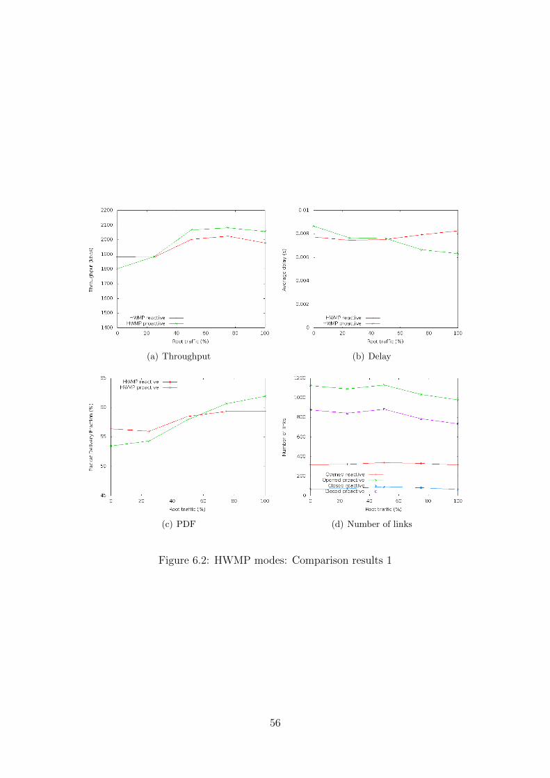
(a) Throughput (b) Delay
(c) PDF (d) Number of links
Figure 6.2: HWMP modes: Comparison results 1
56
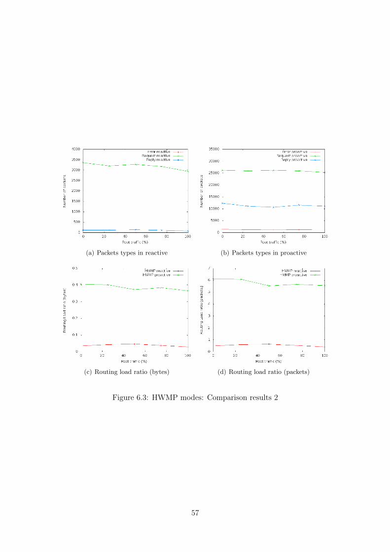
(a) Packets types in reactive (b) Packets types in proactive
(c) Routing load ratio (bytes) (d) Routing load ratio (packets)
Figure 6.3: HWMP modes: Comparison results 2
57

Chapter 7
Conclusions and future work
In this research, a detailed studio of HWMP routing capabilities has been presented.
The implementation of mesh networking in NS-3 has been checked and tested in order
to simulate with as much accuracy as possible the different environments.
In chapter 5, a comparison between HWMP and AODV has been performed to know
the benefits of the MAC-based routing capabilities in front of the commonly used
multihop routing protocol in which HWMP is based, AODV. The results show that
layer 2 routing presents an important advantage in terms of end-to-end delay and
routing load. Difference that increases even more when the number of nodes and
connections is high.
On the other hand, both protocols obtain similar results in terms of packet delivery
fraction. However, in some congestion situations the airtime link metric performs
slightly worse than a normal hop count metric. Despite this difference from which the
routing metric is responsible, we can conclude that the routing at MAC layer clearly
shows benefits in front of the conventional layer 3 routing. This benefits could be of a
high importance when real time applications are used.
In chapter 6, both HWMP operation modes have been discussed to determine in which
environments each one is more suitable. Their performances have been tested in differ-
ent situations of internal and external network traffic. It is concluded that when more
than the half of the traffic is internal, the reactive mode is a better option, while when
59
it is external the best choice is to use the proactive tree based mode. This results can
be used to define a guideline in the ways of use of HWMP.
As future work, more possible scenarios for comparison could be analyzed using dif-
ferent applications and mobility models in order to extract more general conclusions.
Also the physical deployment of a mesh network (for example using the open80211s
linux implementation [4]) would help to check the accuracy of the NS-3 simulator and
its mesh modules, and to know in which aspect they should be improved.
An study on different routing metrics to use with HWMP could be also an important
field of research which would help to improve its performance. ALM presents some
interesting features but, as it has been proved in this research, the hop count metric
works better in some situations.
Another possible line of work could be to develop some mesh networking unsupported
features of NS-3. Thus, it will be possible to define a more complete and complex
environment to test a complete system using a mesh structure. The main features to
develop could be the Mesh Coordinated Channel Access or the Mesh Access Point and
Portal capabilities.
60
Appendix A
AODV routing protocol
The AODV (Ad-hoc On demand Distance Vector) is an on-demand reactive protocol
that uses the distant vector routing algorithm. In AODV, the source node and the
intermediate nodes store the next-hop information corresponding to each flow for data
packet transmission. This protocol uses the messages RREQ (Route Request), RREP
(Route Replies) and RERR (Route Errors).
In AODV, nodes discover routes in request-response cycles. A node requests a route
to a destination by broadcasting an RREQ message to all its neighbors. When a node
receives an RREQ message but does not have a route to the requested destination,
it broadcasts again the RREQ message. Also, it remembers a reverse-route to the
requesting node which can be used to forward subsequent responses to this RREQ.
This process repeats until the RREQ reaches a node that has a valid route to the
destination. This node (which can be the destination itself) responds with an RREP
message. This RREP is unicast along the reverse-routes of the intermediate nodes until
it reaches the original requesting node. Thus, at the end of this request-response cycle
a bidirectional route is established between the requesting node and the destination.
When a node loses connectivity to its next hop, the node invalidates its route by sending
an RERR to all nodes that potentially received its RREP.
The major difference between AODV and other on-demand routing protocols is that
it uses a destination sequence number (DSN) to determine an up-to-date path to the
destination. A node updates its path information only if the DSN of the current
61
packet received is greater than the last DSN stored at the node. A RREQ carries
the source identifier (SrcID), the destination identifier (DestID), the source sequence
number (SSN), the DSN, the broadcast identifier (BcastID), and the time to live (TTL)
field. DSN indicates the freshness of the route that is accepted by the source. When
an intermediate node receives a RREQ, it either forwards it or prepares a RREP if
it has a valid route to the destination. The validity of a route at the intermediate
node is determined by comparing the sequence number at the intermediate node with
the destination sequence number in the RREQ. If a RREQ is received multiple times,
which is indicated by the BcastID-SrcID pair, the duplicate copies are discarded.
All intermediate nodes having valid routes to the destination, or the destination node
itself, are allowed to send RREP packets to the source. Every intermediate node, while
forwarding a RREQ, enters the previous node address and its BcastID. A timer is used
to delete this entry in case a RREP is not received before the timer expires. This
helps in storing an active path at the intermediate node as AODV does not employ
source routing of data packets. When a node receives a RREP, information about the
previous node from which the packet was received is also stored in order to forward
the data packet to this next node as the next hop toward the destination.
All nodes active in the network transmit periodically hello messages (considered as
special RREP messages). If one node does not receive a hello from the neighbors it
means that the connection has been lost and they modify their routing table deleting
that path. It also sends a RRER to the other neighbor nodes that used that path.
Advantages and disadvantages
The AODV routing protocol is designed for networks with populations of tens to thou-
sands of mobile nodes and can handle low, moderate and relatively high mobility rates,
as well as a variety of data traffic levels. AODV has also been designed to reduce the
dissemination of control traffic and eliminate overhead on data traffic, in order to im-
prove scalability and performance.
One of the disadvantages of this protocol is that intermediate nodes can lead to in-
consistent routes if the source sequence number is very old and the intermediate nodes
62
have a higher but not the latest destination sequence number, thereby having stale
entries. Also multiple RREP packets in response to a single RREQ packet can lead to
heavy control overhead. Another disadvantage of AODV is that the periodic beaconing
leads to unnecessary bandwidth consumption.
63

Appendix B
NS-3 802.11s modules
In this appendix, the modules implemented in C++ and how they interconnect with
each other is presented following the description in 3.3.
B.1 MeshHelper
void SetSpreadInterfaceChannels
Parameters: (ChannelPolicy)
Set the channel policy which can be SPREAD CHANNELS or ZERO CHANNEL:
Spread or not spread frequency channels of MP interfaces. If set to true different
non-overlapping 20MHz frequency channels will be assigned to different mesh point
interfaces.
void SetStackInstaller
Parameters: (std::string type, std::string n0 = ””, const AttributeValue &v0 = Empty-
AttributeValue (),...)
You need to tell which Mesh stack do you want, in this case Dot11sStack, so you can
use the characteristics of the 802.11s. n0 and v0 are the name and the value of the
65
attribute to set, respectively. For example you can set the root node in the mesh
network.
void SetNumberOfInterfaces
Parameters: (uint32 t nInterfaces)
Set a number of interfaces in a mesh network.
NetDeviceContainer Install
Parameters: (const WifiPhyHelper &phyHelper, NodeContainer c)
Install 802.11s mesh device and protocols on given node list. The phyHelper is the
Wifi PHY helper and c is the list of nodes to install. This function returns the list of
created mesh point devices, see MeshPointDevice (see next section).
void SetMacType
Parameters: ( std::string n0=””, const AttributeValue &v0 = EmptyAttributeValue
(),...)
Uses the class MeshWifiInterfaceMac and n0 and v0 are the name and the value of the
attribute to set, respectively. The values that can be set are the next ones:
• BeaconInterval : Beacon Interval. Initial value: 0.5 seconds
• RandomStart : Window when beacon generating starts (uniform random) in sec-
onds. Initial value: 0.5 seconds
• BeaconGeneration: Enable/Disable Beaconing. Initial value: enabled
• TxOkHeader : The header of successfully transmitted packet.
• TxErrHeader : The header of unsuccessfully transmitted packet.
66
This class uses the RegularWifiMac class where you can set the QoS support which
enable 802.11e/WMM-style (By default is disable). And at the same time this class
has as parent class WifiMac which we can use to modify values like CTS timeout, ACK
timeout, SIFTS, EIFS-DIFS, duration of a slot, PIFS or the Ssid.
void SetRemoteStationManager
Parameters: (std::string type, std::string n0=””, const AttributeValue &v0 = Empty-
AttributeValue (),...)
With this function, using the variable type we define which station manager do we want.
A part from a constant bit rate value, the following rate control algorithms implemented
in NS-3: AARF, AARF-CD, AMRR, ARF, CARA, Ideal, Minstrel, ONOE and RRAA.
The one selected by default is the ARF.
They all use has as parent class WifiRemoteStationManager, and using the n0 and v0
you can set the maximum number of retransmission attempts for an RTS and data
packets as well as the threshold to decide when to use a RTS/CTS handshake before
sending a data packet and the one to decide when to fragment them. As described in
IEEE Std. 802.11-2007, Section 9.2.6. and 9.4. This value will not have any effect
on some rate control algorithms. Here we can also set a wifi mode for non-unicast
transmissions.
void SetNumberOfInterfaces
Parameters: (uint32 t nInterfaces)
Set a number of interfaces in a mesh network.
void SetStandard
Parameters: (enum WifiPhyStandard standard)
67
Allows you to select the following standards: 802.11 with 5 or 10 Mhz, 802.11a and
802.11b. The one set by default is the 802.11a.
B.2 MeshPointDevice
Mesh point is a virtual net device which is responsible for aggregating and coordinating
real devices (mesh interfaces), and hosting all mesh-related level 2 protocols. One
of hosted L2 protocols must implement L2RoutingProtocol interface and is used for
packets forwarding.
From the level 3 point of view MeshPointDevice is similar to a bridge network device,
but the packets, which going through may be changed (because L2 protocols may
require their own headers or tags).
void AddInterface
Parameters: (Ptr< NetDevice > port)
Attach new interface to the station. Interface must support 48-bit MAC address and
only MeshPointDevice can have IP address, but not individual interfaces.
bool SetMtu
Parameters: (const uint16 t mtu)
Set the MAC-level Maximum Transmission Unit in bytes and returns whether the MTU
value was within legal bounds. Override for default MTU defined on a per-type basis.
void SetRoutingProtocol
Parameters: (Ptr< MeshL2RoutingProtocol > protocol)
68
Register the mesh routing protocol to be used by this mesh point. Protocol must be
already installed on this mesh point.
B.3 HWMP
Here a list of all the parameters which can be configure in this implementation of
HWMP and their values by default is presented.
• RandomStart : Random delay at first proactive PREQ. Initial value: 100ms
• MaxQueueSize: Maximum number of packets we can store when resolving route.
Initial value: 255
• Dot11MeshHWMPmaxPREQretries : Maximum number of retries before we sup-
pose the destination to be unreachable. Initial value: 3
• Dot11MeshHWMPnetDiameterTraversalTime: Time we suppose the packet to
go from one edge of the network to another. Initial value: 102.4ms
• Dot11MeshHWMPpreqMinInterval : Minimal interval between to successive PREQs.
Initial value: 102.4ms
• Dot11MeshHWMPperrMinInterval : Minimal interval between to successive PERRs.
Initial value: 102.4ms
• Dot11MeshHWMPactiveRootTimeout : Lifetime of proactive routing information
(PREQ). Initial value: 5120ms
• Dot11MeshHWMPactivePathTimeout : Lifetime of reactive routing information.
Initial value: 5120ms
• Dot11MeshHWMPpathToRootInterval : Interval between two successive proactive
PREQs. Initial value: 2048ms
• Dot11MeshHWMPrannInterval : Lifetime of proactive routing information (RANN).
Initial value: 5120ms
69
• MaxTtl : Initial value of Time To Live field. Initial value: 32
• UnicastPerrThreshold : Maximum number of PERR receivers, when we send a
PERR as a chain of unicasts. Initial value: 32
• UnicastPreqThreshold : Maximum number of PREQ receivers, when we send a
PREQ as a chain of unicasts. Initial value: 1
• UnicastDataThreshold : Maximum number of broadcast receivers, when we send
a broadcast as a chain of unicasts. Initial value: 1
• DoFlag : Destination only HWMP flag. Initial value: false
• RfFlag : Reply and forward flag. Initial value: true
Through this class we can decide if we want to use the root structure or not in th
proactive PREQ mechanism. For this the function SetRoot and UnsetRoot are avail-
able.
B.4 Peer Management Protocol
Here a list of all the parameters which can be configure in this implementation of PMP
and their values by default is presented.
• MaxNumberOfPeerLinks : Maximum number of peer links. Initial value: 32
• MaxBeaconShiftValue: Maximum number of TUs for beacon shifting. Initial
value: 15
• EnableBeaconCollisionAvoidance: Enable/Disable Beacon collision avoidance.
Initial value: true
When we install the PMP in a device, we also define the Mesh ID where it will belong
using the function SetMeshId.
70
B.5 Peer Link
As the last configurable characteristics of HWMP, here is presented the peer link model
for the Peer Management protocol.
• RetryTimeout : Retry timeout. Initial value: 41 ms
• HoldingTimeout : Holding timeout. Initial value: 41 ms
• ConfirmTimeout : Confirm timeout. Initial value: 41 ms
• MaxRetries : Maximum number of retries. Initial value: 4
• MaxBeaconLoss : Maximum number of lost beacons before link will be closed.
Initial value: 2
• MaxPacketFailure: Maximum number of failed packets before link will be closed.
Initial value: 2
After several test, all these parameters were modified to adapt them to the scenario
characteristics and some of them do not use its default value. This is explained in the
next chapter.
71

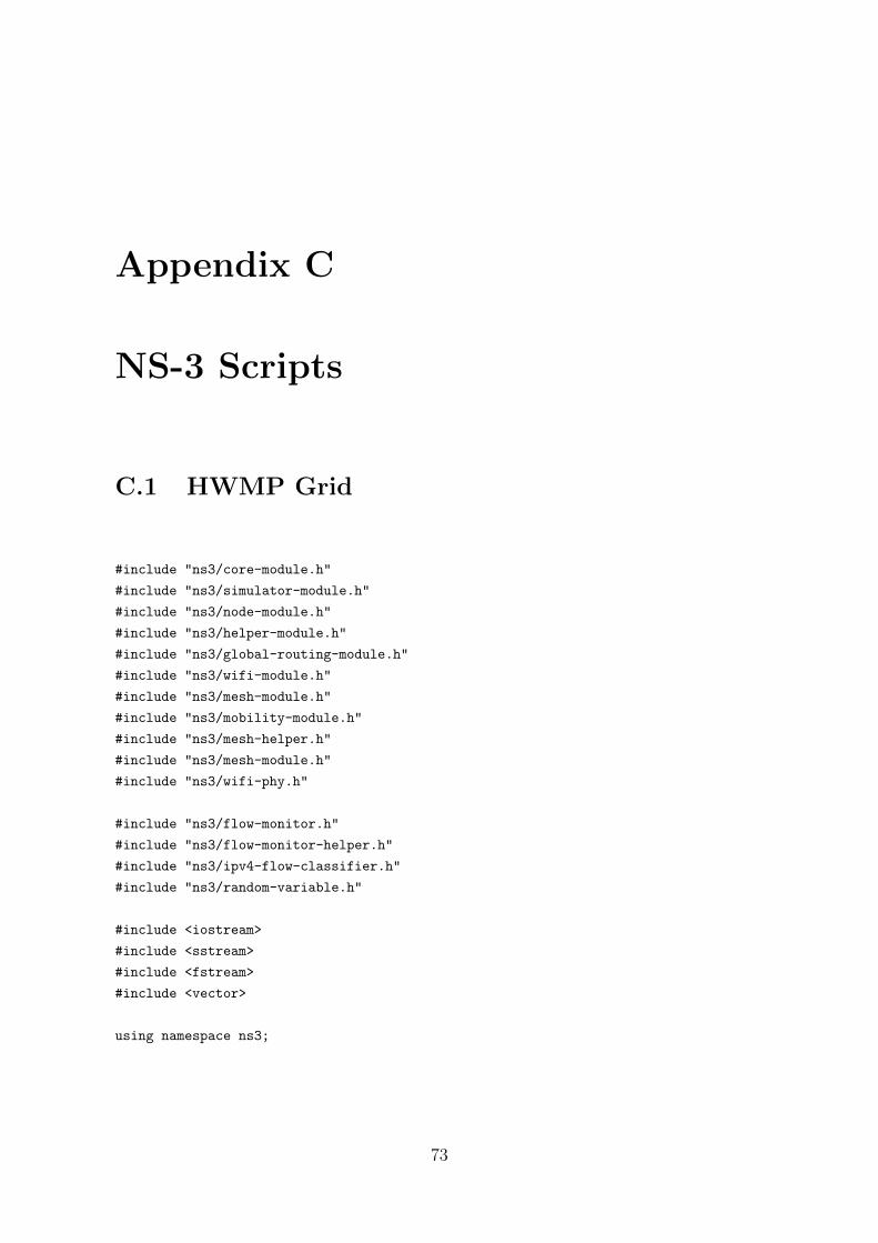
Appendix C
NS-3 Scripts
C.1 HWMP Grid
#include "ns3/core-module.h"
#include "ns3/simulator-module.h"
#include "ns3/node-module.h"
#include "ns3/helper-module.h"
#include "ns3/global-routing-module.h"
#include "ns3/wifi-module.h"
#include "ns3/mesh-module.h"
#include "ns3/mobility-module.h"
#include "ns3/mesh-helper.h"
#include "ns3/mesh-module.h"
#include "ns3/wifi-phy.h"
#include "ns3/flow-monitor.h"
#include "ns3/flow-monitor-helper.h"
#include "ns3/ipv4-flow-classifier.h"
#include "ns3/random-variable.h"
#include <iostream>
#include <sstream>
#include <fstream>
#include <vector>
using namespace ns3;
73
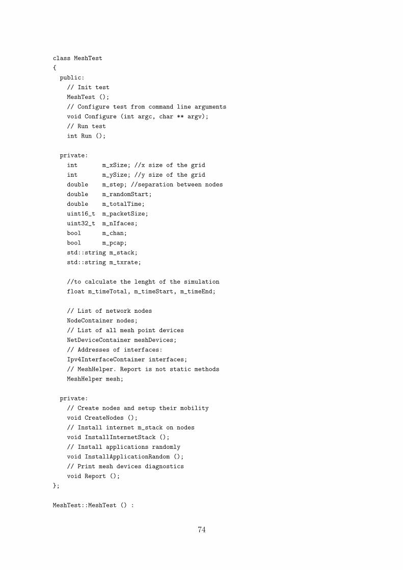
class MeshTest
{
public:
// Init test
MeshTest ();
// Configure test from command line arguments
void Configure (int argc, char ** argv);
// Run test
int Run ();
private:
int m_xSize; //x size of the grid
int m_ySize; //y size of the grid
double m_step; //separation between nodes
double m_randomStart;
double m_totalTime;
uint16_t m_packetSize;
uint32_t m_nIfaces;
bool m_chan;
bool m_pcap;
std::string m_stack;
std::string m_txrate;
//to calculate the lenght of the simulation
float m_timeTotal, m_timeStart, m_timeEnd;
// List of network nodes
NodeContainer nodes;
// List of all mesh point devices
NetDeviceContainer meshDevices;
// Addresses of interfaces:
Ipv4InterfaceContainer interfaces;
// MeshHelper. Report is not static methods
MeshHelper mesh;
private:
// Create nodes and setup their mobility
void CreateNodes ();
// Install internet m_stack on nodes
void InstallInternetStack ();
// Install applications randomly
void InstallApplicationRandom ();
// Print mesh devices diagnostics
void Report ();
};
MeshTest::MeshTest () :
74
m_xSize (5),
m_ySize (5),
m_step (170),
m_randomStart (0.1),
m_totalTime (240),
m_packetSize (1024),
m_nIfaces (1),
m_chan (false),
m_pcap (false),
m_stack ("ns3::Dot11sStack"),
m_txrate ("150kbps")
{
}
void
MeshTest::Configure (int argc, char *argv[])
{
CommandLine cmd;
cmd.AddValue ("m_xSize", "m_xSize", m_xSize);
cmd.AddValue ("m_ySize", "m_ySize", m_ySize);
cmd.AddValue ("m_txrate", "m_txrate", m_txrate);
cmd.Parse (argc, argv);
}
void MeshTest::CreateNodes ()
{
int i, j;
double m_txpower = 18.0; // dbm
// Calculate m_ySize*m_xSize stations grid topology
double position_x = 0;
double position_y = 0;
ListPositionAllocator myListPositionAllocator;
for (i = 1; i <= m_xSize; i++){
for (j = 1; j <= m_ySize; j++){
std::cout << "Node at x = " << position_x << ", y = " << position_y << "\n";
Vector3D n_pos (position_x, position_y, 0.0);
myListPositionAllocator.Add(n_pos);
position_y += m_step;
}
position_y = 0;
position_x += m_step;
}
75
// Create the nodes
nodes.Create (m_xSize*m_ySize);
// Configure YansWifiChannel
YansWifiPhyHelper WifiPhy = YansWifiPhyHelper::Default ();
WifiPhy.Set ("EnergyDetectionThreshold", DoubleValue (-89.0) );
WifiPhy.Set ("CcaMode1Threshold", DoubleValue (-62.0) );
WifiPhy.Set ("TxGain", DoubleValue (1.0) );
WifiPhy.Set ("RxGain", DoubleValue (1.0) );
WifiPhy.Set ("TxPowerLevels", UintegerValue (1) );
WifiPhy.Set ("TxPowerEnd", DoubleValue (m_txpower) );
WifiPhy.Set ("TxPowerStart", DoubleValue (m_txpower) );
WifiPhy.Set ("RxNoiseFigure", DoubleValue (7.0) );
YansWifiChannelHelper WifiChannel;
WifiChannel.SetPropagationDelay ("ns3::ConstantSpeedPropagationDelayModel");
WifiChannel.AddPropagationLoss ("ns3::LogDistancePropagationLossModel","Exponent",
StringValue ("2.7"));
WifiPhy.SetChannel (WifiChannel.Create ());
// Configure the parameters of the Peer Link
Config::SetDefault ("ns3::dot11s::PeerLink::MaxBeaconLoss", UintegerValue (20));
Config::SetDefault ("ns3::dot11s::PeerLink::MaxRetries", UintegerValue (4));
Config::SetDefault ("ns3::dot11s::PeerLink::MaxPacketFailure", UintegerValue (5));
// Configure the parameters of the Peer Management Protocol
Config::SetDefault ("ns3::dot11s::PeerManagementProtocol::EnableBeaconCollision-
Avoidance",BooleanValue (false));
// Configure the parameters of the HWMP
Config::SetDefault ("ns3::dot11s::HwmpProtocol::Dot11MeshHWMPactivePathTimeout",
TimeValue (Seconds (100)));
Config::SetDefault ("ns3::dot11s::HwmpProtocol::Dot11MeshHWMPactiveRootTimeout",
TimeValue (Seconds (100)));
Config::SetDefault ("ns3::dot11s::HwmpProtocol::Dot11MeshHWMPmaxPREQretries",
UintegerValue (5));
Config::SetDefault ("ns3::dot11s::HwmpProtocol::UnicastPreqThreshold",
UintegerValue (10));
Config::SetDefault ("ns3::dot11s::HwmpProtocol::UnicastDataThreshold",
UintegerValue (5));
Config::SetDefault ("ns3::dot11s::HwmpProtocol::DoFlag", BooleanValue (true));
Config::SetDefault ("ns3::dot11s::HwmpProtocol::RfFlag", BooleanValue (false));
// Stack installer creates all protocols and install them to mesh point device
76
mesh = MeshHelper::Default ();
mesh.SetStandard (WIFI_PHY_STANDARD_80211a);
mesh.SetMacType ("RandomStart", TimeValue (Seconds(m_randomStart)));
mesh.SetRemoteStationManager ("ns3::ConstantRateWifiManager", "DataMode",
StringValue ("OfdmRate6Mbps"), "RtsCtsThreshold", UintegerValue (2500));
// Set number of interfaces - default is single-interface mesh point
mesh.SetNumberOfInterfaces (m_nIfaces);
mesh.SetStackInstaller (m_stack);
//If multiple channels is activated
if (m_chan) {
mesh.SetSpreadInterfaceChannels (MeshHelper::SPREAD_CHANNELS);
}
else {
mesh.SetSpreadInterfaceChannels (MeshHelper::ZERO_CHANNEL);
}
// Install protocols and return container if MeshPointDevices
meshDevices = mesh.Install (WifiPhy, nodes);
// Place the protocols in the positions calculated before
MobilityHelper mobility;
mobility.SetPositionAllocator(&myListPositionAllocator);
mobility.SetMobilityModel ("ns3::ConstantPositionMobilityModel");
mobility.Install (nodes);
}
void MeshTest::InstallInternetStack ()
{
//Install the internet protocol stack on all nodes
InternetStackHelper internetStack;
internetStack.Install (nodes);
//Assign IP addresses to the devices interfaces
Ipv4AddressHelper address;
address.SetBase ("192.168.1.0", "255.255.255.0");
interfaces = address.Assign (meshDevices);
}
void MeshTest::InstallApplicationRandom ()
{
// Create as many connections as nodes has the grid
int m_nconn = m_xSize * m_ySize;
int i=0;
77
int m_source, m_dest, m_dest_port;
char num [2];
char onoff [7];
char sink [6];
double start_time, stop_time, duration;
// Set the parameters of the onoff application
Config::SetDefault ("ns3::OnOffApplication::PacketSize", UintegerValue
(m_packetSize));
Config::SetDefault ("ns3::OnOffApplication::DataRate", StringValue (m_txrate));
ApplicationContainer apps [m_nconn];
UniformVariable rand_nodes (0,m_ySize*m_xSize-1);
UniformVariable rand_port (49000,49100);
// 50 seconds for transitori are left at the beginning.
UniformVariable a(50,m_totalTime-15);
for (i = 0; i < m_nconn; i++){
start_time = a.GetValue();
ExponentialVariable b(30);
duration = b.GetValue()+1;
// If the exponential variable gives us a value that added to the start time
// is greater than the maximum permitted, this is changed for the maximum
// 10 seconds are left at the end to calculate well the statistics of each flow
if ( (start_time + duration) > (m_totalTime - 10)){
stop_time = m_totalTime-10;
}else{
stop_time = start_time + duration;
}
// Create different names for the connections
// (we can not use vectors for OnOffHelper)
strcpy(onoff,"onoff");
strcpy(sink,"sink");
sprintf(num,"%d",i);
strcat(onoff,num);
strcat(sink,num);
// Set random variables of the destination (server) and destination port.
m_dest = rand_nodes.GetInteger (0,m_ySize*m_xSize-1);
m_dest_port = rand_port.GetInteger (49000,49100);
78
// Set random variables of the source (client)
m_source = rand_nodes.GetInteger (0,m_ySize*m_xSize-1);
// Client and server can not be the same node.
while (m_source == m_dest){
m_source = rand_nodes.GetInteger (0,m_ySize*m_xSize-1);
}
// Plot the connection values
std::cout << "\n\t Node "<< m_source << " to " << m_dest;
std::cout << "\n Start_time: " << start_time << "s";
std::cout << "\n Stop_time: " << stop_time << "s\n";
// Define UDP traffic for the onoff application
OnOffHelper onoff ("ns3::UdpSocketFactory", Address (InetSocketAddress
(interfaces.GetAddress (m_dest), m_dest_port)));
onoff.SetAttribute ("OnTime", RandomVariableValue (ConstantVariable (1)));
onoff.SetAttribute ("OffTime", RandomVariableValue (ConstantVariable (0)));
apps[i] = onoff.Install (nodes.Get(m_source));
apps[i].Start (Seconds (start_time));
apps[i].Stop (Seconds (stop_time));
// Create a packet sink to receive the packets
PacketSinkHelper sink ("ns3::UdpSocketFactory",InetSocketAddress
(interfaces.GetAddress (m_dest), 49001));
apps[i] = sink.Install (nodes.Get (m_dest));
apps[i].Start (Seconds (1.0));
}
}
int MeshTest::Run ()
{
CreateNodes ();
InstallInternetStack ();
InstallApplicationRandom ();
// Install FlowMonitor on all nodes
FlowMonitorHelper flowmon;
Ptr<FlowMonitor> monitor = flowmon.InstallAll();
m_timeStart=clock();
Simulator::Schedule (Seconds(m_totalTime), & MeshTest::Report, this);
Simulator::Stop (Seconds (m_totalTime));
Simulator::Run ();
79
// Define variables to calculate the metrics
int k=0;
int totaltxPackets = 0;
int totalrxPackets = 0;
double totaltxbytes = 0;
double totalrxbytes = 0;
double totaldelay = 0;
double totalrxbitrate = 0;
double difftx, diffrx;
double pdf_value, rxbitrate_value, txbitrate_value, delay_value;
double pdf_total, rxbitrate_total, delay_total;
//Print per flow statistics
monitor->CheckForLostPackets ();
Ptr<Ipv4FlowClassifier> classifier = DynamicCast<Ipv4FlowClassifier>
(flowmon.GetClassifier ());
std::map<FlowId, FlowMonitor::FlowStats> stats = monitor->GetFlowStats ();
for (std::map<FlowId, FlowMonitor::FlowStats>::const_iterator i = stats.begin ();
i != stats.end (); ++i)
{
Ipv4FlowClassifier::FiveTuple t = classifier->FindFlow (i->first);
difftx = i->second.timeLastTxPacket.GetSeconds() -
i->second.timeFirstTxPacket.GetSeconds();
diffrx = i->second.timeLastRxPacket.GetSeconds() -
i->second.timeFirstRxPacket.GetSeconds();
pdf_value = (double) i->second.rxPackets / (double) i->second.txPackets * 100;
txbitrate_value = (double) i->second.txBytes * 8 / 1024 / difftx;
if (i->second.rxPackets != 0){
rxbitrate_value = (double)i->second.rxPackets * m_packetSize * 8 /
1024 / diffrx;
delay_value = (double) i->second.delaySum.GetSeconds() /
(double) i->second.rxPackets;
}
else{
rxbitrate_value = 0;
delay_value = 0;
}
// We are only interested in the metrics of the data flows
if ((!t.destinationAddress.IsSubnetDirectedBroadcast("255.255.255.0")))
{
k++;
80
// Plot the statistics for each data flow
std::cout << "\nFlow " << k << " (" << t.sourceAddress << " -> "
<< t.destinationAddress << ")\n";
//std::cout << "Tx Packets: " << i->second.txPackets << "\n";
//std::cout << "Rx Packets: " << i->second.rxPackets << "\n";
//std::cout << "Lost Packets: " << i->second.lostPackets << "\n";
//std::cout << "Dropped Packets: " << i->second.packetsDropped.size() << "\n";
std::cout << "PDF: " << pdf_value << " %\n";
std::cout << "Average delay: " << delay_value << "s\n";
std::cout << "Rx bitrate: " << rxbitrate_value << " kbps\n";
std::cout << "Tx bitrate: " << txbitrate_value << " kbps\n\n";
// Acumulate for average statistics
totaltxPackets += i->second.txPackets;
totaltxbytes += i->second.txBytes;
totalrxPackets += i->second.rxPackets;
totaldelay += i->second.delaySum.GetSeconds();
totalrxbitrate += rxbitrate_value;
totalrxbytes += i->second.rxBytes;
}
}
// Average all nodes statistics
if (totaltxPackets != 0){
pdf_total = (double) totalrxPackets / (double) totaltxPackets * 100;
}
else{
pdf_total = 0;
}
if (totalrxPackets != 0){
rxbitrate_total = totalrxbitrate;
delay_total = (double) totaldelay / (double) totalrxPackets;
}
else{
rxbitrate_total = 0;
delay_total = 0;
}
//print all nodes statistics
std::cout << "\nTotal PDF: " << pdf_total << " %\n";
std::cout << "Total Rx bitrate: " << rxbitrate_total << " kbps\n";
std::cout << "Total Delay: " << delay_total << " s\n";
//print all nodes statistics in files
81
std::ostringstream os;
os << "1_HWMP_PDF.txt";
std::ofstream of (os.str().c_str(), ios::out | ios::app);
of << pdf_total << "\n";
of.close ();
std::ostringstream os2;
os2 << "1_HWMP_Delay.txt";
std::ofstream of2 (os2.str().c_str(), ios::out | ios::app);
of2 << delay_total << "\n";
of2.close ();
std::ostringstream os3;
os3 << "1_HWMP_Throu.txt";
std::ofstream of3 (os3.str().c_str(), ios::out | ios::app);
of3 << rxbitrate_total << "\n";
of3.close ();
Simulator::Destroy ();
m_timeEnd=clock();
m_timeTotal=(m_timeEnd - m_timeStart)/(double) CLOCKS_PER_SEC;
std::cout << "\n*** Simulation time: " << m_timeTotal << "s\n\n";
return 0;
}
void MeshTest::Report ()
{
// Using this function we print detailed statistics of each mesh point device
// These statistics are used later with an AWK files to extract routing metrics
unsigned n (0);
for (NetDeviceContainer::Iterator i = meshDevices.Begin ();
i != meshDevices.End (); ++i, ++n)
{
std::ostringstream os;
//os << "mp-report1-" << n << ".xml";
os << "mp-report.xml";
std::ofstream of;
of.open (os.str().c_str(), ios::out | ios::app);
if (! of.is_open ())
{
std::cerr << "Error: Can’t open file " << os.str() << "\n";
return;
}
mesh.Report (*i, of);
82
of.close ();
}
n = 0;
}
int main (int argc, char *argv[])
{
MeshTest t;
t.Configure (argc, argv);
return t.Run();
}
C.2 AODV Grid
#includes are the same as in the previous script
using namespace ns3;
class MeshTest
{
public:
// Init test
MeshTest ();
// Configure test from command line arguments
void Configure (int argc, char ** argv);
// Run test
int Run ();
private:
int m_xSize; //x size of the grid
int m_ySize; //y size of the grid
double m_step; //separation between nodes
double m_totalTime;
uint16_t m_packetSize;
bool m_pcap;
std::string m_txrate;
double m_txrate_dob;
//to calculate the lenght of the simulation
float m_timeTotal, m_timeStart, m_timeEnd;
83
// List of network nodes
NodeContainer nodes;
// List of all wifi devices
NetDeviceContainer wifiDevices;
//Addresses of interfaces:
Ipv4InterfaceContainer interfaces;
// MeshHelper. Report is not static methods
WifiHelper wifi_aodv;
private:
// Create nodes and setup their mobility
void CreateNodes ();
// Install internet m_stack on nodes
void InstallInternetStack ();
// Install applications randomly
void InstallApplicationRandom ();
};
MeshTest::MeshTest () :
m_xSize (5),
m_ySize (5),
m_step (170),
m_totalTime (240),
m_packetSize (1024),
m_pcap (false),
m_txrate ("150kbps"),
m_txrate_dob (150) //needed in kbps for the trace file
{
}
void
MeshTest::Configure (int argc, char *argv[])
{
CommandLine cmd;
cmd.AddValue ("m_xSize", "m_xSize", m_xSize);
cmd.AddValue ("m_ySize", "m_ySize", m_ySize);
cmd.AddValue ("m_txrate", "m_txrate", m_txrate);
cmd.AddValue ("m_txrate_dob", "m_txrate_dob", m_txrate_dob);
cmd.Parse (argc, argv);
}
void MeshTest::CreateNodes ()
{
int i, j;
double m_txpower = 18.0; // dbm
// Calculate m_ySize*m_xSize stations grid topology
84
double position_x = 0;
double position_y = 0;
ListPositionAllocator myListPositionAllocator;
for (i = 1; i <= m_xSize; i++){
for (j = 1; j <= m_ySize; j++){
std::cout << "Node at x = " << position_x << ", y = " << position_y << "\n";
Vector3D n_pos (position_x, position_y, 0.0);
myListPositionAllocator.Add(n_pos);
position_y += m_step;
}
position_y = 0;
position_x += m_step;
}
// Create the nodes
nodes.Create (m_xSize*m_ySize);
// Configure YansWifiChannel
YansWifiPhyHelper WifiPhy = YansWifiPhyHelper::Default ();
WifiPhy.Set ("EnergyDetectionThreshold", DoubleValue (-89.0) );
WifiPhy.Set ("CcaMode1Threshold", DoubleValue (-62.0) );
WifiPhy.Set ("TxGain", DoubleValue (1.0) );
WifiPhy.Set ("RxGain", DoubleValue (1.0) );
WifiPhy.Set ("TxPowerLevels", UintegerValue (1) );
WifiPhy.Set ("TxPowerEnd", DoubleValue (m_txpower) );
WifiPhy.Set ("TxPowerStart", DoubleValue (m_txpower) );
WifiPhy.Set ("RxNoiseFigure", DoubleValue (7.0) );
YansWifiChannelHelper WifiChannel;
WifiChannel.SetPropagationDelay ("ns3::ConstantSpeedPropagationDelayModel");
WifiChannel.AddPropagationLoss ("ns3::LogDistancePropagationLossModel","Exponent",
StringValue ("2.7"));
WifiPhy.SetChannel (WifiChannel.Create ());
wifi_aodv.SetStandard (WIFI_PHY_STANDARD_80211a);
wifi_aodv.SetRemoteStationManager ("ns3::ConstantRateWifiManager", "DataMode",
StringValue ("OfdmRate6Mbps"), "RtsCtsThreshold", UintegerValue (2500));
// Install protocols and return container
NqosWifiMacHelper wifiMac = NqosWifiMacHelper::Default();
wifiMac.SetType ("ns3::AdhocWifiMac");
wifiDevices = wifi_aodv.Install (WifiPhy, wifiMac, nodes);
85
// Place the protocols in the positions calculated before
MobilityHelper mobility;
mobility.SetPositionAllocator(&myListPositionAllocator);
mobility.SetMobilityModel ("ns3::ConstantPositionMobilityModel");
mobility.Install (nodes);
}
void MeshTest::InstallInternetStack ()
{
//configure AODV
AodvHelper aodv;
aodv.Set ("AllowedHelloLoss", UintegerValue (20));
aodv.Set ("HelloInterval", TimeValue (Seconds (3)));
aodv.Set ("RreqRetries", UintegerValue (5));
aodv.Set ("ActiveRouteTimeout", TimeValue (Seconds (100)));
aodv.Set ("DestinationOnly", BooleanValue (true));
//Install the internet protocol stack on all nodes
InternetStackHelper internetStack;
internetStack.SetRoutingHelper (aodv);
internetStack.Install (nodes);
//Assign IP addresses to the devices interfaces (m_nIfaces)
Ipv4AddressHelper address;
address.SetBase ("192.168.1.0", "255.255.255.0");
interfaces = address.Assign (wifiDevices);
}
void MeshTest::InstallApplicationRandom ()
{
// Create as many connections as nodes has the grid
int m_nconn = m_xSize * m_ySize;
int i=0;
int m_source, m_dest, m_dest_port;
char num [2];
char onoff [7];
char sink [6];
double start_time, stop_time, duration;
// Set the parameters of the onoff application
Config::SetDefault ("ns3::OnOffApplication::PacketSize",
UintegerValue (m_packetSize));
Config::SetDefault ("ns3::OnOffApplication::DataRate", StringValue (m_txrate));
ApplicationContainer apps [m_nconn];
86
UniformVariable rand_nodes (0,m_ySize*m_xSize-1);
UniformVariable rand_port (49000,49100);
// 50 seconds for transitori are left at the beginning.
UniformVariable a(50,m_totalTime-15);
for (i = 0; i < m_nconn; i++){
start_time = a.GetValue();
ExponentialVariable b(30);
duration = b.GetValue()+1;
// If the exponential variable gives us a value that added to the start time
// is greater than the maximum permitted, this is changed for the maximum
// 10 seconds are left at the end to calculate well the statistics of each flow
if ( (start_time + duration) > (m_totalTime - 10)){
stop_time = m_totalTime-10;
}else{
stop_time = start_time + duration;
}
// Create different names for the connections
// (we can not use vectors for OnOffHelper)
strcpy(onoff,"onoff");
strcpy(sink,"sink");
sprintf(num,"%d",i);
strcat(onoff,num);
strcat(sink,num);
// Set random variables of the destination (server) and destination port.
m_dest = rand_nodes.GetInteger (0,m_ySize*m_xSize-1);
m_dest_port = rand_port.GetInteger (49000,49100);
// Set random variables of the source (client)
m_source = rand_nodes.GetInteger (0,m_ySize*m_xSize-1);
// Client and server can not be the same node.
while (m_source == m_dest){
m_source = rand_nodes.GetInteger (0,m_ySize*m_xSize-1);
}
// Plot the connection values
std::cout << "\n\t Node "<< m_source << " to " << m_dest;
std::cout << "\n Start_time: " << start_time << "s";
std::cout << "\n Stop_time: " << stop_time << "s\n";
87
// Define UDP traffic for the onoff application
OnOffHelper onoff ("ns3::UdpSocketFactory", Address (InetSocketAddress
(interfaces.GetAddress (m_dest), m_dest_port)));
onoff.SetAttribute ("OnTime", RandomVariableValue (ConstantVariable (1)));
onoff.SetAttribute ("OffTime", RandomVariableValue (ConstantVariable (0)));
apps[i] = onoff.Install (nodes.Get(m_source));
apps[i].Start (Seconds (start_time));
apps[i].Stop (Seconds (stop_time));
// Create a packet sink to receive the packets
PacketSinkHelper sink ("ns3::UdpSocketFactory",InetSocketAddress
(interfaces.GetAddress (m_dest), 49001));
apps[i] = sink.Install (nodes.Get (m_dest));
apps[i].Start (Seconds (1.0));
}
}
int MeshTest::Run ()
{
CreateNodes ();
InstallInternetStack ();
InstallApplicationRandom ();
// Install FlowMonitor on all nodes
FlowMonitorHelper flowmon;
Ptr<FlowMonitor> monitor = flowmon.InstallAll();
m_timeStart=clock();
Simulator::Stop (Seconds (m_totalTime));
Simulator::Run ();
// Define variables to calculate the metrics
int k=0;
int totaltxPackets = 0;
int totalrxPackets = 0;
int totaltxPacketsR = 0;
int totalrxPacketsR = 0;
double totaltxbytes = 0;
double totalrxbytes = 0;
double totaltxbytesR = 0;
double totalrxbytesR = 0;
double totaldelay = 0;
double totalrxbitrate = 0;
88
double difftx, diffrx;
double pdf_value, rxbitrate_value, txbitrate_value, delay_value;
double pdf_total, rxbitrate_total, delay_total;
double RL_rx_pack, RL_tx_pack, RL_rx_bytes, RL_tx_bytes;
//Print per flow statistics
monitor->CheckForLostPackets ();
Ptr<Ipv4FlowClassifier> classifier = DynamicCast<Ipv4FlowClassifier>
(flowmon.GetClassifier ());
std::map<FlowId, FlowMonitor::FlowStats> stats = monitor->GetFlowStats ();
for (std::map<FlowId, FlowMonitor::FlowStats>::const_iterator i = stats.begin ();
i != stats.end (); ++i)
{
Ipv4FlowClassifier::FiveTuple t = classifier->FindFlow (i->first);
difftx = i->second.timeLastTxPacket.GetSeconds() -
i->second.timeFirstTxPacket.GetSeconds();
diffrx = i->second.timeLastRxPacket.GetSeconds() -
i->second.timeFirstRxPacket.GetSeconds();
pdf_value = (double) i->second.rxPackets / (double) i->second.txPackets * 100;
txbitrate_value = (double) i->second.txBytes * 8 / 1024 / difftx;
if (i->second.rxPackets != 0){
rxbitrate_value = (double) i->second.rxPackets * m_packetSize * 8
/ 1024 / diffrx;
delay_value = (double) i->second.delaySum.GetSeconds() /
(double) i->second.rxPackets;
}
else{
rxbitrate_value = 0;
delay_value = 0;
}
// We are only interested in the metrics of the data flows. This AODV
// implementation create other flows with routing information at low bitrates,
// so a margin is defined to ensure that only our data flows are filtered.
if ( (!t.destinationAddress.IsSubnetDirectedBroadcast("255.255.255.0")) &&
(txbitrate_value > m_txrate_dob/1.2) && (rxbitrate_value < m_txrate_dob*1.2))
{
k++;
std::cout << "\nFlow " << k << " (" << t.sourceAddress << " -> "
<< t.destinationAddress << ")\n";
//std::cout << "Tx Packets: " << i->second.txPackets << "\n";
//std::cout << "Rx Packets: " << i->second.rxPackets << "\n";
//std::cout << "Lost Packets: " << i->second.lostPackets << "\n";
89
//std::cout << "Dropped Packets: " << i->second.packetsDropped.size() << "\n";
std::cout << "PDF: " << pdf_value << " %\n";
std::cout << "Average delay: " << delay_value << "s\n";
std::cout << "Rx bitrate: " << rxbitrate_value << " kbps\n";
std::cout << "Tx bitrate: " << txbitrate_value << " kbps\n\n";
// Acumulate for average statistics
totaltxPackets += i->second.txPackets;
totaltxbytes += i->second.txBytes;
totalrxPackets += i->second.rxPackets;
totaldelay += i->second.delaySum.GetSeconds();
totalrxbitrate += rxbitrate_value;
totalrxbytes += i->second.rxBytes;
}
else{
totaltxbytesR += i->second.txBytes;
totalrxbytesR += i->second.rxBytes;
totaltxPacketsR += i->second.txPackets;
totalrxPacketsR += i->second.rxPackets;
}
}
//Average all nodes statistics
if (totaltxPackets != 0){
pdf_total = (double) totalrxPackets / (double) totaltxPackets * 100;
RL_tx_pack = (double) totaltxPacketsR / (double) totaltxPackets;
RL_tx_bytes = totaltxbytesR / totaltxbytes;
}
else{
pdf_total = 0;
RL_tx_pack = 0;
RL_tx_bytes = 0;
}
if (totalrxPackets != 0){
rxbitrate_total = totalrxbitrate;
delay_total = (double) totaldelay / (double) totalrxPackets;
RL_rx_pack = (double) totalrxPacketsR / (double) totalrxPackets;
RL_rx_bytes = totalrxbytesR / totalrxbytes;
}
else{
rxbitrate_total = 0;
delay_total = 0;
RL_rx_pack = 0;
RL_rx_bytes = 0;
}
90
// Print all nodes statistics
std::cout << "\nTotal PDF: " << pdf_total << " %\n";
std::cout << "Total Rx bitrate: " << rxbitrate_total << " kbps\n";
std::cout << "Total Delay: " << delay_total << " s\n";
// Print all nodes statistics in files
std::ostringstream os;
os << "1_AODV_PDF.txt";
std::ofstream of (os.str().c_str(), ios::out | ios::app);
of << pdf_total << "\n";
std::ostringstream os2;
os2 << "1_AODV_Delay.txt";
std::ofstream of2 (os2.str().c_str(), ios::out | ios::app);
of2 << delay_total << "\n";
std::ostringstream os3;
os3 << "1_AODV_Throu.txt";
std::ofstream of3 (os3.str().c_str(), ios::out | ios::app);
of3 << rxbitrate_total << "\n";
std::ostringstream os5;
os5 << "1_AODV_RL_RxBytes.txt";
std::ofstream of5 (os5.str().c_str(), ios::out | ios::app);
of5 << RL_rx_bytes << "\n";
std::ostringstream os7;
os7 << "1_AODV_RL_RxPack.txt";
std::ofstream of7 (os7.str().c_str(), ios::out | ios::app);
of7 << RL_rx_pack << "\n";
of.close (); of2.close (); of3.close (); of5.close (); of7.close ();
Simulator::Destroy ();
m_timeEnd=clock();
m_timeTotal=(m_timeEnd - m_timeStart)/(double) CLOCKS_PER_SEC;
std::cout << "\n*** Simulation time: " << m_timeTotal << "s\n\n";
return 0;
}
int main (int argc, char *argv[])
{
MeshTest t;
t.Configure (argc, argv);
return t.Run();
}
91
C.3 HWMP different modes
#include "ns3/core-module.h"
#include "ns3/simulator-module.h"
#include "ns3/node-module.h"
#include "ns3/helper-module.h"
#include "ns3/global-routing-module.h"
#include "ns3/wifi-module.h"
#include "ns3/mesh-module.h"
#include "ns3/mobility-module.h"
#include "ns3/mesh-helper.h"
#include "ns3/mesh-module.h"
#include "ns3/wifi-phy.h"
#include "ns3/flow-monitor.h"
#include "ns3/flow-monitor-helper.h"
#include "ns3/ipv4-flow-classifier.h"
#include "ns3/random-variable.h"
#include "ns3/boolean.h"
#include <iostream>
#include <sstream>
#include <fstream>
#include <vector>
using namespace ns3;
class MeshTest
{
public:
// Init test
MeshTest ();
// Configure test from command line arguments
void Configure (int argc, char ** argv);
// Run test
int Run ();
private:
int m_nnodes; // number of nodes
int m_nconn; // number of connections
int m_nconnR; // number of connections to the root
double m_step;
92
double m_randomStart;
double m_totalTime;
uint16_t m_packetSize;
uint32_t m_nIfaces;
bool m_chan;
bool m_pcap;
std::string m_stack;
int m_reactive;
std::string m_txrate;
//to calculate the lenght of the simulation
float m_timeTotal, m_timeStart, m_timeEnd;
// List of network nodes
NodeContainer nodes;
// List of all mesh point devices
NetDeviceContainer meshDevices;
//Addresses of interfaces:
Ipv4InterfaceContainer interfaces;
// MeshHelper. Report is not static methods
MeshHelper mesh;
// List of network nodes
NodeContainer nodesC;
// List of all mesh point devices
NetDeviceContainer meshDevicesC;
//Addresses of interfaces:
Ipv4InterfaceContainer interfacesC;
// MeshHelper. Report is not static methods
MeshHelper meshC;
private:
// Create nodes and setup their mobility
void CreateNodes ();
// Install internet m_stack on nodes
void InstallInternetStack ();
// Install applications randomly
void InstallApplicationRandom ();
// Print mesh devices diagnostics
void Report ();
// Create nodes and setup their mobility
void CreateNodesC ();
// Install internet m_stack on nodes
void InstallInternetStackC ();
};
93
MeshTest::MeshTest () :
m_nnodes (25),
m_nconn (28),
m_nconnR (0),
m_step (720),
m_randomStart (0.5),
m_totalTime (240),
m_packetSize (1024),
m_nIfaces (1),
m_chan (false),
m_pcap (false),
m_stack ("ns3::Dot11sStack"),
m_reactive (1),
m_txrate ("120kbps")
{
}
void
MeshTest::Configure (int argc, char *argv[])
{
CommandLine cmd;
cmd.AddValue ("m_step", "Separation", m_step);
cmd.AddValue ("m_nconn", "Number of connections", m_nconn);
cmd.AddValue ("m_nconnR", "Number of root connections", m_nconnR);
cmd.AddValue ("m_reactive", "Mode type", m_reactive);
cmd.Parse (argc, argv);
}
void MeshTest::CreateNodes ()
{
std::string m_root;
double m_txpower = 18.0; // dbm
// Calculate nnodes stations random topology
nodes.Create (nnodes);
// Setup mobility - static rectangle topology
MobilityHelper mobility;
mobility.SetPositionAllocator ("ns3::RandomRectanglePositionAllocator",
"X", RandomVariableValue (UniformVariable (0, m_step)),
"Y", RandomVariableValue (UniformVariable (0, m_step/2)));
mobility.SetMobilityModel ("ns3::ConstantPositionMobilityModel");
mobility.Install (nodes);
// Configure YansWifiChannel
YansWifiPhyHelper WifiPhy = YansWifiPhyHelper::Default ();
94
WifiPhy.Set ("EnergyDetectionThreshold", DoubleValue (-89.0) );
WifiPhy.Set ("CcaMode1Threshold", DoubleValue (-62.0) );
WifiPhy.Set ("TxGain", DoubleValue (1.0) );
WifiPhy.Set ("RxGain", DoubleValue (1.0) );
WifiPhy.Set ("TxPowerLevels", UintegerValue (1) );
WifiPhy.Set ("TxPowerEnd", DoubleValue (m_txpower) );
WifiPhy.Set ("TxPowerStart", DoubleValue (m_txpower) );
WifiPhy.Set ("RxNoiseFigure", DoubleValue (7.0) );
YansWifiChannelHelper WifiChannel;
WifiChannel.SetPropagationDelay ("ns3::ConstantSpeedPropagationDelayModel");
WifiChannel.AddPropagationLoss ("ns3::LogDistancePropagationLossModel","Exponent",
StringValue ("2.7"));
WifiPhy.SetChannel (WifiChannel.Create ());
// Configure the parameters of the Peer Link
Config::SetDefault ("ns3::dot11s::PeerLink::MaxBeaconLoss", UintegerValue (20));
Config::SetDefault ("ns3::dot11s::PeerLink::MaxRetries", UintegerValue (4));
Config::SetDefault ("ns3::dot11s::PeerLink::MaxPacketFailure", UintegerValue (5));
// Configure the parameters of the Peer Management Protocol
Config::SetDefault ("ns3::dot11s::PeerManagementProtocol::EnableBeaconCollision-
Avoidance", BooleanValue (false));
// Configure the parameters of the HWMP
Config::SetDefault ("ns3::dot11s::HwmpProtocol::Dot11MeshHWMPactivePathTimeout",
TimeValue (Seconds (100)));
Config::SetDefault ("ns3::dot11s::HwmpProtocol::Dot11MeshHWMPactiveRootTimeout",
TimeValue (Seconds (100)));
Config::SetDefault ("ns3::dot11s::HwmpProtocol::Dot11MeshHWMPmaxPREQretries",
UintegerValue (5));
Config::SetDefault ("ns3::dot11s::HwmpProtocol::UnicastPreqThreshold",
UintegerValue (10));
Config::SetDefault ("ns3::dot11s::HwmpProtocol::UnicastDataThreshold",
UintegerValue (5));
Config::SetDefault ("ns3::dot11s::HwmpProtocol::DoFlag", BooleanValue (false));
Config::SetDefault ("ns3::dot11s::HwmpProtocol::RfFlag", BooleanValue (true));
// Create mesh helper and set stack installer to it
// Stack installer creates all needed protocols and install them to device
mesh = MeshHelper::Default ();
mesh.SetStandard (WIFI_PHY_STANDARD_80211a);
mesh.SetMacType ("RandomStart", TimeValue (Seconds(m_randomStart)));
mesh.SetRemoteStationManager ("ns3::ConstantRateWifiManager", "DataMode",
StringValue ("OfdmRate6Mbps"), "RtsCtsThreshold", UintegerValue (2500));
95
// Set number of interfaces - default is single-interface mesh point
mesh.SetNumberOfInterfaces (m_nIfaces);
mesh.SetStackInstaller (m_stack);
if (m_reactive == 1) {
//If reactive mode is on, we do not use "Root" attribute
m_root = "Reactive mode";
mesh.SetStackInstaller (m_stack);
}
else{
//If proactive mode is on, we define node 6 as root
m_root = "00:00:00:00:00:06";
mesh.SetStackInstaller (m_stack, "Root", Mac48AddressValue
(Mac48Address (m_root.c_str ())));
}
std::cout << "\n\t root: " << m_root << "\n";
//If multiple channels is activated
if (m_chan) {
mesh.SetSpreadInterfaceChannels (MeshHelper::SPREAD_CHANNELS);
}
else {
mesh.SetSpreadInterfaceChannels (MeshHelper::ZERO_CHANNEL);
}
// Install protocols and return container if MeshPointDevices
meshDevices = mesh.Install (WifiPhy, nodes);
}
void MeshTest::CreateNodesC ()
{
// We only create the extra node
nodesC.Create (1);
YansWifiPhyHelper WifiPhy = YansWifiPhyHelper::Default ();
YansWifiChannelHelper WifiChannel;
WifiChannel.SetPropagationDelay ("ns3::ConstantSpeedPropagationDelayModel");
WifiChannel.AddPropagationLoss ("ns3::LogDistancePropagationLossModel","Exponent",
StringValue ("2.7"));
WifiPhy.SetChannel (WifiChannel.Create ());
meshC = MeshHelper::Default ();
meshDevicesC = meshC.Install (WifiPhy, nodesC);
// This extra node is placed far away to not interfere
Vector3D n1_posC (m_step*3, m_step*3, m_step*3);
96
ListPositionAllocator myListPositionAllocatorC;
myListPositionAllocatorC.Add(n1_posC);
MobilityHelper mobilityC;
mobilityC.SetPositionAllocator(&myListPositionAllocatorC);
mobilityC.SetMobilityModel ("ns3::ConstantPositionMobilityModel");
mobilityC.Install (nodesC);
}
void MeshTest::InstallInternetStack ()
{
//Install the internet protocol stack on all nodes
InternetStackHelper internetStack;
internetStack.Install (nodes);
//Assign IP addresses to the devices interfaces (m_nIfaces)
Ipv4AddressHelper address;
address.SetBase ("192.168.1.0", "255.255.255.0");
interfaces = address.Assign (meshDevices);
}
void MeshTest::InstallInternetStackC ()
{
//Install the internet protocol stack on all nodes
InternetStackHelper internetStack;
internetStack.Install (nodesC);
//Assign IP addresses to the extra node is also from another network
Ipv4AddressHelper address;
address.SetBase ("192.168.2.0", "255.255.255.0");
interfacesC = address.Assign (meshDevicesC);
}
void MeshTest::InstallApplicationRandom ()
{
int i=0;
int ir=0;
int m_source, m_dest, m_dest_port;
char num [2];
char onoff [7];
char sink [6];
double start_time, stop_time, duration;
97
// Set the parameters of the onoff application
Config::SetDefault ("ns3::OnOffApplication::PacketSize",
UintegerValue (m_packetSize));
Config::SetDefault ("ns3::OnOffApplication::DataRate", StringValue (m_txrate));
ApplicationContainer apps [m_nconn];
UniformVariable rand_nodes (0,nnodes-1);
UniformVariable rand_port (49000,49100);
// 50 seconds for transitori are left at the beginning.
UniformVariable a(50,m_totalTime-15);
for (i = 0; i < m_nconn; i++){
start_time = a.GetValue();
ExponentialVariable b(25);
duration = b.GetValue()+1;
// If the exponential variable gives us a value that added to the start time
// is greater than the maximum permitted, this is changed for the maximum
// 10 seconds are left at the end to calculate well the statistics of each flow
if ( (start_time + duration) > (m_totalTime - 10)){
stop_time = m_totalTime-10;
}else{
stop_time = start_time + duration;
}
//create different names for the connections
//(we can not use vectors for OnOffHelper)
strcpy(onoff,"onoff");
strcpy(sink,"sink");
sprintf(num,"%d",i);
strcat(onoff,num);
strcat(sink,num);
//set random variables of the destination (server) and destination port.
m_dest = rand_nodes.GetInteger (0,nnodes-1);
m_dest_port = rand_port.GetInteger (49000,49100);
//change the destination to the root if more root traffic is required
if (ir < m_nconnR){
m_dest = 5;
ir++;
}
98
// Set random variables of the source (client).
// Client and server can not be the same node.
m_source = rand_nodes.GetInteger (0,nnodes-1);
while (m_source == m_dest){
m_source = rand_nodes.GetInteger (0,nnodes-1);
}
// Plot the connection values
std::cout << "\n\t Node "<< m_source << " to " << m_dest;
std::cout << "\n Start_time: " << start_time << "s";
std::cout << "\n Stop_time: " << stop_time << "s\n";
// Define UDP traffic for the onoff application
OnOffHelper onoff ("ns3::UdpSocketFactory", Address (InetSocketAddress
(interfaces.GetAddress (m_dest), m_dest_port)));
onoff.SetAttribute ("OnTime", RandomVariableValue (ConstantVariable (1)));
onoff.SetAttribute ("OffTime", RandomVariableValue (ConstantVariable (0)));
apps[i] = onoff.Install (nodes.Get(m_source));
apps[i].Start (Seconds (start_time));
apps[i].Stop (Seconds (stop_time));
// Create a packet sink to receive these packets
PacketSinkHelper sink ("ns3::UdpSocketFactory",InetSocketAddress
(interfaces.GetAddress (m_dest), 49001));
apps[i] = sink.Install (nodes.Get (m_dest));
apps[i].Start (Seconds (1.0));
}
}
int MeshTest::Run ()
{
CreateNodes ();
InstallInternetStack ();
// In this mesh implementation when the proactive mode is used, when creating
// the root node this counts as if there was another node. Thus, when using
// the seed for the random variables it gives different values in reactive
// and proactive mode. To solve this, in reactive mode a fake mode that does
// not communicate neither interfere is created.
if (m_reactive == 1) {
CreateNodesC ();
InstallInternetStackC ();
std::cout << "\n Node: Installing extra node to compensate the root\n";
}
99
InstallApplicationRandom ();
// Install FlowMonitor on all nodes
FlowMonitorHelper flowmon;
Ptr<FlowMonitor> monitor = flowmon.InstallAll();
m_timeStart=clock();
Simulator::Schedule (Seconds(m_totalTime), & MeshTest::Report, this);
Simulator::Stop (Seconds (m_totalTime));
Simulator::Run ();
// Define variables to calculate the metrics
int k=0;
int totaltxPackets = 0;
int totalrxPackets = 0;
double totaltxbytes = 0;
double totalrxbytes = 0;
double totaldelay = 0;
double totalrxbitrate = 0;
double difftx, diffrx;
double pdf_value, rxbitrate_value, txbitrate_value, delay_value;
double pdf_total, rxbitrate_total, delay_total;
//Print per flow statistics
monitor->CheckForLostPackets ();
Ptr<Ipv4FlowClassifier> classifier = DynamicCast<Ipv4FlowClassifier>
(flowmon.GetClassifier ());
std::map<FlowId, FlowMonitor::FlowStats> stats = monitor->GetFlowStats ();
for (std::map<FlowId, FlowMonitor::FlowStats>::const_iterator i = stats.begin ();
i != stats.end (); ++i)
{
Ipv4FlowClassifier::FiveTuple t = classifier->FindFlow (i->first);
difftx = i->second.timeLastTxPacket.GetSeconds() -
i->second.timeFirstTxPacket.GetSeconds();
diffrx = i->second.timeLastRxPacket.GetSeconds() -
i->second.timeFirstRxPacket.GetSeconds();
pdf_value = (double) i->second.rxPackets / (double) i->second.txPackets * 100;
txbitrate_value = (double) i->second.txBytes * 8 / 1024 / difftx;
if (i->second.rxPackets != 0){
rxbitrate_value = (double)i->second.rxPackets * m_packetSize * 8 /
1024 / diffrx;
100
delay_value = (double) i->second.delaySum.GetSeconds() /
(double) i->second.rxPackets;
}
else{
rxbitrate_value = 0;
delay_value = 0;
}
// We are only interested in the metrics of the data flows
if ((!t.destinationAddress.IsSubnetDirectedBroadcast("255.255.255.0")))
{
k++;
// Plot the statistics for each data flow
std::cout << "\nFlow " << k << " (" << t.sourceAddress << " -> "
<< t.destinationAddress << ")\n";
//std::cout << "Tx Packets: " << i->second.txPackets << "\n";
//std::cout << "Rx Packets: " << i->second.rxPackets << "\n";
//std::cout << "Lost Packets: " << i->second.lostPackets << "\n";
//std::cout << "Dropped Packets: " << i->second.packetsDropped.size() << "\n";
std::cout << "PDF: " << pdf_value << " %\n";
std::cout << "Average delay: " << delay_value << "s\n";
std::cout << "Rx bitrate: " << rxbitrate_value << " kbps\n";
std::cout << "Tx bitrate: " << txbitrate_value << " kbps\n\n";
// Acumulate for average statistics
totaltxPackets += i->second.txPackets;
totaltxbytes += i->second.txBytes;
totalrxPackets += i->second.rxPackets;
totaldelay += i->second.delaySum.GetSeconds();
totalrxbitrate += rxbitrate_value;
totalrxbytes += i->second.rxBytes;
}
}
// Average all nodes statistics
if (totaltxPackets != 0){
pdf_total = (double) totalrxPackets / (double) totaltxPackets * 100;
}
else{
pdf_total = 0;
}
if (totalrxPackets != 0){
rxbitrate_total = totalrxbitrate;
delay_total = (double) totaldelay / (double) totalrxPackets;
}
101
else{
rxbitrate_total = 0;
delay_total = 0;
}
//print all nodes statistics
std::cout << "\nTotal PDF: " << pdf_total << " %\n";
std::cout << "Total Rx bitrate: " << rxbitrate_total << " kbps\n";
std::cout << "Total Delay: " << delay_total << " s\n";
//print all nodes statistics in files
std::ostringstream os;
os << "1_HWMP_PDF.txt";
std::ofstream of (os.str().c_str(), ios::out | ios::app);
of << pdf_total << "\n";
of.close ();
std::ostringstream os2;
os2 << "1_HWMP_Delay.txt";
std::ofstream of2 (os2.str().c_str(), ios::out | ios::app);
of2 << delay_total << "\n";
of2.close ();
std::ostringstream os3;
os3 << "1_HWMP_Throu.txt";
std::ofstream of3 (os3.str().c_str(), ios::out | ios::app);
of3 << rxbitrate_total << "\n";
of3.close ();
Simulator::Destroy ();
m_timeEnd=clock();
m_timeTotal=(m_timeEnd - m_timeStart)/(double) CLOCKS_PER_SEC;
std::cout << "\n*** Simulation time: " << m_timeTotal << "s\n\n";
return 0;
}
void MeshTest::Report ()
{
// Using this function we print detailed statistics of each mesh point device
// These statistics are used later with an AWK files to extract routing metrics
unsigned n (0);
for (NetDeviceContainer::Iterator i = meshDevices.Begin ();
i != meshDevices.End (); ++i, ++n)
102
{
std::ostringstream os;
//os << "mp-report1-" << n << ".xml";
os << "mp-report.xml";
std::ofstream of;
of.open (os.str().c_str(), ios::out | ios::app);
if (! of.is_open ())
{
std::cerr << "Error: Can’t open file " << os.str() << "\n";
return;
}
mesh.Report (*i, of);
of.close ();
}
n = 0;
}
int main (int argc, char *argv[])
{
MeshTest t;
t.Configure (argc, argv);
return t.Run();
}
103

Bibliography
[1] C. Perkins, E. Belding-Royer, and S. Das, “Ad hoc on-demand distance vector
(AODV) routing,” IETF RFC 3561, 2003.
[2] I. Akyildiz and X. Wang, “A survey on wireless mesh networks,” Communications
Magazine, IEEE, vol. 43, pp. S23 – S30, sept. 2005.
[3] “IEEE Draft Standard for Information Technology-Telecommunications and in-
formation exchange between systems-Local and metropolitan area networks-
Specific requirements-Part 11: Wireless LAN Medium Access Control (MAC) and
Physical Layer (PHY) specifications-Amendment 10: Mesh Networking,” IEEE
P802.11s/D10.0, March 2011, pp. 1 –379, 29 2011.
[4] open80211s, “www.open80211s.org/.”
[5] M.-X. Hu and G.-S. Kuo, “Delay and throughput Analysis of IEEE 802.11s Net-
works,” in Communications Workshops, 2008. ICC Workshops ’08. IEEE Inter-
national Conference on, pp. 73 –78, may 2008.
[6] J. Yan, S. Zhang, Y. Sun, and H. Feng, “Performance Analysis of the IEEE
802.11s Common Channel Framework,” in Wireless Communications, Networking
and Mobile Computing, 2008. WiCOM ’08. 4th International Conference on, pp. 1
–4, oct. 2008.
[7] S. Ghannay, S. Gammar, and F. Kamoun, “Performance comparison of hop count
and radio aware path selection protocols in IEEE 802.11s WLAN mesh networks,”
in Wireless Days, 2008. WD ’08. 1st IFIP, pp. 1 –5, nov. 2008.
105
[8] K. Yang, J. feng Ma, and Z. hui Miao, “Hybrid Routing Protocol for Wireless
Mesh Network,” in Computational Intelligence and Security, 2009. CIS ’09. In-
ternational Conference on, vol. 1, pp. 547 –551, dec. 2009.
[9] L. J. S. Cuenca, “802.11s based wireless mesh network (WMN) test-bed,” 2010.
[10] Y.-D. Lin, S.-L. Tsao, S.-L. Chang, S.-Y. Cheng, and C.-Y. Ku, “Design issues and
experimental studies of wireless LAN Mesh,” Wireless Communications, IEEE,
vol. 17, pp. 32 –40, april 2010.
[11] P. Pandey, S. Satish, J. Kuri, and H. Dagale, “Implementation of IEEE 802.11s
mesh nodes with enhanced features,” in Mobile Adhoc and Sensor Systems, 2009.
MASS ’09. IEEE 6th International Conference on, pp. 639 –644, oct. 2009.
[12] X. Wang and A. O. Lim, “IEEE 802.11s wireless mesh networks: Framework and
challenges,” Ad Hoc Networks, 2007.
[13] G. Hiertz, D. Denteneer, S. Max, R. Taori, J. Cardona, L. Berlemann, and
B. Walke, “IEEE 802.11s: The WLAN Mesh Standard,” Wireless Communica-
tions, IEEE, vol. 17, pp. 104 –111, february 2010.
[14] Y. Chen and S. Emeott, “MDA simulation study: Robustness to non-MDA inter-
ferers,” IEEE 802 Plenary Meeting, 2007.
[15] R. Carrano, L. Magalha andes, D. Saade, and C. Albuquerque, “IEEE 802.11s
Multihop MAC: A Tutorial,” Communications Surveys Tutorials, IEEE, vol. 13,
pp. 52 –67, quarter 2011.
[16] “Draft STANDARD for Information Technology-Telecommunications and infor-
mation exchange between systems-Local and metropolitan area networks-Specific
requirements-Part 11: Wireless LAN Medium Access Control (MAC) and Physical
Layer (PHY) specifications Amendment 10: Mesh Networking,” IEEE Unapproved
Draft Std P802.11s/D3.0, Mar 2009, 2009.
[17] K. Andreev and P. Boyko, “IEEE 802.11s mesh networking NS-3 model,” 2009.
[18] “NS-3 network simulator official website, www.nsnam.org.”
[19] “NS-3 doxygen documentation, www.nsnam.org/doxygen-release/index.html.”
106
[20] J. B. et al., “A performance comparison of ad-hoc multihop wireless networks
routing protocols,” Proc. IEEE/ACM MOBICOM, 1998.
[21] G. Carneiro, P. Fortuna, and M. Ricardo, “Flowmonitor - a network monitoring
framework for the network simulator 3,” NSTOOLS, 2009.
[22] K. Jain, J. Padhye, V. N. Padmanabhan, and L. Qiu, “Impact of interference on
multi-hop wireless network performance,” Proc. ACM/IEEE MOBICOM, 2003.
[23] A. Iyer, C. Rosenberg, and A. Karnik, “What is the right model for wireless
channel interference?,” Wireless Communications, IEEE Transactions on, vol. 8,
pp. 2662 –2671, may 2009.
[24] S. Ray, J. Carruthers, and D. Starobinski, “RTS/CTS-induced congestion in ad
hoc wireless LANs,” in Wireless Communications and Networking, 2003. WCNC
2003. 2003 IEEE, vol. 3, pp. 1516 –1521 vol.3, march 2003.
107

List of Figures
2.1 The 802.11s network architecture . . . . . . . . . . . . . . . . . . . . . 7
2.2 Peer link establishment . . . . . . . . . . . . . . . . . . . . . . . . . . . 9
2.3 HWMP on-demand route discovery. . . . . . . . . . . . . . . . . . . . . 13
2.4 HWMP proactive PREQ route discovery. . . . . . . . . . . . . . . . . . 14
2.5 IEEE 802.11s frame structure . . . . . . . . . . . . . . . . . . . . . . . 17
4.1 Transmission rate vs. distance . . . . . . . . . . . . . . . . . . . . . . . 29
4.2 HWMP vs number of hops . . . . . . . . . . . . . . . . . . . . . . . . . 30
4.3 Interference Scenarios 1a and 1b . . . . . . . . . . . . . . . . . . . . . . 31
4.4 Interference Scenarios 2a and 2b . . . . . . . . . . . . . . . . . . . . . . 33
5.1 Routing metric evaluation . . . . . . . . . . . . . . . . . . . . . . . . . 38
5.2 Scalability: delay evolution over the grids . . . . . . . . . . . . . . . . . 40
5.3 Scalability: detailed delay of a connection . . . . . . . . . . . . . . . . 42
5.4 Scalability: routing load ratio evolution over the grids . . . . . . . . . . 44
5.5 Scalability results in a 3x3 grid . . . . . . . . . . . . . . . . . . . . . . 44
5.6 Scalability results in a 4x4 grid . . . . . . . . . . . . . . . . . . . . . . 45
109
5.7 Scalability results in a 5x5 grid . . . . . . . . . . . . . . . . . . . . . . 46
5.8 Scalability results in a 6x6 grid . . . . . . . . . . . . . . . . . . . . . . 47
6.1 Destination only flag evaluation in HWMP . . . . . . . . . . . . . . . . 52
6.2 HWMP modes: Comparison results 1 . . . . . . . . . . . . . . . . . . . 56
6.3 HWMP modes: Comparison results 2 . . . . . . . . . . . . . . . . . . . 57
110
List of Tables
2.1 ALM constants . . . . . . . . . . . . . . . . . . . . . . . . . . . . . . . 10
2.2 Frame types . . . . . . . . . . . . . . . . . . . . . . . . . . . . . . . . . 15
4.1 Data rate for each transmission rate . . . . . . . . . . . . . . . . . . . . 29
5.1 HWMP and AODV parameters . . . . . . . . . . . . . . . . . . . . . . 37
5.2 Scalability: detailed results of a connection . . . . . . . . . . . . . . . . 41
6.1 HWMP parameters . . . . . . . . . . . . . . . . . . . . . . . . . . . . . 50
111


![(d, ,]) Fuzzy Logic - UPCommons](https://static.documents.pub/doc/80x56/6207321549d709492c2ee10d/d-fuzzy-logic-upcommons.jpg)


