IEEE ROBOTICS AND AUTOMATION LETTERS. PREPRINT VERSION. ACCEPTED JANUARY, 2018 1

Distance-Aware Dynamically Weighted Roadmapsfor Motion Planning in Unknown Environments

Adrian Knobloch, Nikolaus Vahrenkamp, Mirko Wachter and Tamim Asfour

Abstract—The paper presents and evaluates a Distance AwareDynamic Roadmap (DA-DRM) algorithm as an extension of theDynamic Roadmap (DRM) approach. In contrast to previouswork, the algorithm is capable of planning collision-free tra-jectories while considering the distance to obstacles, even inunknown environments which are perceived by the robot’s depthcamera system. The algorithm makes use of a voxel distancegrid which is updated based on perceptual information acquiredfrom the robot’s perception system. The distance information isconsidered as a cost factor during the roadmap search and it isconsidered in a post-processing step that is used for trajectorysmoothing. We evaluate the DA-DRM algorithm in simulationand in a real-world experiments with the humanoid robotARMAR-III. In addition, we compare our algorithm against theDRM and the RRT-Connect algorithm. The results demonstratethe performance of our algorithm in terms of keeping a safetydistance to obstacles, trajectory smoothness as well as the abilityto generate solutions in narrow free space.

Index Terms—Motion and Path Planning Collision Avoidance

I. INTRODUCTION

THE efficient generation of collision-free trajectories for arobot in partly known or even unknown environments is

a challenging task. In contrast to motion planning approaches,which assume a perfect world knowledge, approaches for realworld applications should be able to consider unknown obsta-cles and dynamically changing environments. Hence, planningalgorithms which are capable of integrating perceptual inputare indispensable in open-ended environments. When consid-ering human-robot interaction scenarios, the predictability ofthe robot’s movement is an additional requirement that leadsto higher confidence and acceptance by humans.

Thus, a motion planning algorithm should be aware of thedistance to obstacles to allow generating trajectories with asafety distance to obstacles to avoid collisions which mayoccur due to sensor and actor inaccuracies or to unreliablehand-eye calibration in grasping and manipulation tasks.

We present a motion planning algorithm capable of generat-ing collision-free trajectories based on perceived depth images

Manuscript received: 09/10/2017; Revised 12/16/2017; Accepted01/15/2018.

This paper was recommended for publication by Editor Nancy Amato uponevaluation of the Associate Editor and Reviewers’ comments. The researchleading to these results has received funding from the European UnionsHorizon 2020 Research and Innovation programme under grant agreementNo 643950 (SecondHands).

The authors are with the High Performance HumanoidTechnologies (H2T) Lab, Institute for Anthropomatics andRobotics (IAR), Karlsruhe Institute of Technology (KIT),Germany adrian.knobloch@student.kit.edu,{vahrenkamp,waechter,asfour}@kit.edu

Digital Object Identifier (DOI): see top of this page.

Fig. 1. The scene (top) is used to generate the point cloud shown in thebottom using the depth camera of the ARMAR-III. The adapted roadmapgraph is shown in workspace (bottom). The edge costs which are associatedwith obstacle distance are shown in different colors (low: blue; high: red).

without the need of computer vision algorithms for objectdetection and localization. In addition, the planned motions ofthe Distance Aware Dynamic Roadmap (DA-DRM) algorithmconsiders the obstacle distance in order to avoid movementsthat result in unnecessary low distances to the environment.

II. RELATED WORK

Motion planning has been a highly addressed research topicin robotics in the last decades and a wide variety of algorithmshave been developed. The most common types of planning

2 IEEE ROBOTICS AND AUTOMATION LETTERS. PREPRINT VERSION. ACCEPTED JANUARY, 2018

algorithms are Rapidly-exploring Random Tree (RRT)- andProbabilistic Roadmap (PRM)-based approaches. The RRT issingle-query motion planning algorithm which was developedby Kuffner and LaValle [1] and served as the basis for manyextensions and variations. RRT-based approaches have theadvantage that no preprocessing is needed and that they canbe applied in high-dimensional configuration spaces, and invarious domains. In contrast to such single-query methods,PRM-based approaches are multi-query algorithms. Thesealgorithms require pre-calculated data to plan a collision-free trajectory, but due to the preprocessed data, PRMs canbe queried very efficiently. The standard PRM approach [2]needs collision informations during the preprocessing stagein order to generate the roadmap. Since these informationscannot always be provided in real-world applications, severalalgorithms have been developed to address this issue. Onepossibility is to plan a trajectory for the static part of theenvironment using a PRM and then adapt this trajectory to thedynamic parts [3]. Another approach, which even works forcompletely unknown environments is the Dynamic Roadmap(DRM) algorithm ([4], [5]). As shown by Kallmann andMataric [6], DRMs can be used with a point cloud repre-sentation of the actual scene. This DRM algorithm has beenused in various works, in particular to improve the efficiencyof the approach to make it applicable for online usage ([7],[8], [9], [10], [11], [12]). A critical issue of RRT and PRMbased approaches is the quality of the planned trajectories interms of smoothness and length. Several methods have beenproposed to deal with these issues. For PRM-based algorithms,the quality of the trajectories could be improved by improvingthe roadmap itself ([13], [14]). Other approaches optimize thetrajectory in an post-processing step. This can be achieved byrandomly creating shortcuts on the path [15] with elastic bandalgorithms [16], or the CHOMP approach [17].

III. DISTANCE-AWARE DYNAMIC ROADMAPS

We present a distance-aware dynamic roadmap algorithm,the DA-DRM, which is based on the DRM algorithm [4] andwhich is is able to directly work with point clouds. In thefollowing, we briefly describe the basic DRM approach andour extensions which result in the new DA-DRM algorithm.Finally, we present a post-processing step for the DA-DRMalgorithm, which smooths the generated trajectories whileconsidering the obstacle distance information generated duringplanning.

The DRM algorithm is divided into two steps: an offlineroadmap generation step and the online trajectory generationstep. The roadmap generation consists of the following steps:1) configuration sampling, where we use preferred samplingaround configurations in the main working area as extension,2) generation of the DRM graph using k-nearest neighboursearch, and 3) establishment of the mapping between thevoxelized workspace and the nodes and edges of the graphUsing the resulting roadmap, the online trajectory generationis achieved by the following steps: 1) Calculation of theoccupied workspace voxels, where additionally voxels nextto the occupied voxels and their distance to the blocked part

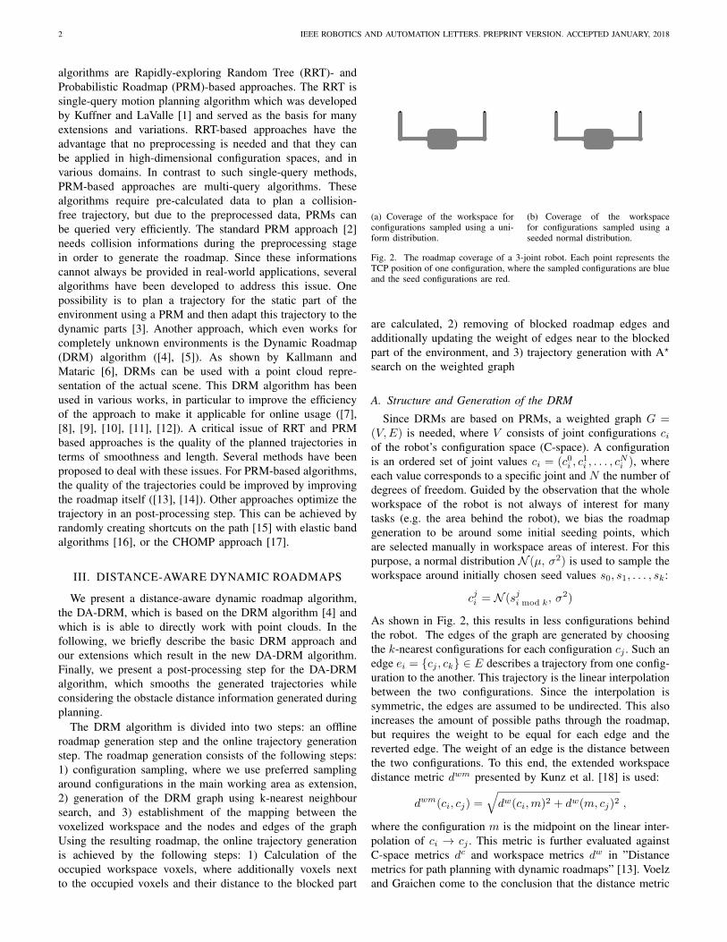
(a) Coverage of the workspace forconfigurations sampled using a uni-form distribution.

(b) Coverage of the workspacefor configurations sampled using aseeded normal distribution.

Fig. 2. The roadmap coverage of a 3-joint robot. Each point represents theTCP position of one configuration, where the sampled configurations are blueand the seed configurations are red.

are calculated, 2) removing of blocked roadmap edges andadditionally updating the weight of edges near to the blockedpart of the environment, and 3) trajectory generation with A?

search on the weighted graph

A. Structure and Generation of the DRM

Since DRMs are based on PRMs, a weighted graph G =(V,E) is needed, where V consists of joint configurations ciof the robot’s configuration space (C-space). A configurationis an ordered set of joint values ci = (c0i , c

1i , . . . , c

Ni ), where

each value corresponds to a specific joint and N the number ofdegrees of freedom. Guided by the observation that the wholeworkspace of the robot is not always of interest for manytasks (e.g. the area behind the robot), we bias the roadmapgeneration to be around some initial seeding points, whichare selected manually in workspace areas of interest. For thispurpose, a normal distribution N (µ, σ2) is used to sample theworkspace around initially chosen seed values s0, s1, . . . , sk:

cji = N (sji mod k, σ2)

As shown in Fig. 2, this results in less configurations behindthe robot. The edges of the graph are generated by choosingthe k-nearest configurations for each configuration cj . Such anedge ei = {cj , ck} ∈ E describes a trajectory from one config-uration to the another. This trajectory is the linear interpolationbetween the two configurations. Since the interpolation issymmetric, the edges are assumed to be undirected. This alsoincreases the amount of possible paths through the roadmap,but requires the weight to be equal for each edge and thereverted edge. The weight of an edge is the distance betweenthe two configurations. To this end, the extended workspacedistance metric dwm presented by Kunz et al. [18] is used:

dwm(ci, cj) =√dw(ci,m)2 + dw(m, cj)2 ,

where the configuration m is the midpoint on the linear inter-polation of ci → cj . This metric is further evaluated againstC-space metrics dc and workspace metrics dw in ”Distancemetrics for path planning with dynamic roadmaps” [13]. Voelzand Graichen come to the conclusion that the distance metric

KNOBLOCH et al.: DISTANCE-AWARE DYNAMICALLY WEIGHTED ROADMAPS FOR MOTION PLANNING IN UNKNOWN ENVIRONMENTS 3

(a) (b) (c) (d)

Fig. 3. The DA-DRM algorithm consists of three stages: 3(a) → 3(b): Calculation of the occupied workspace voxels using point cloud data; 3(b) → 3(c):Adapt the DA-DRM graph to the current state of the environment; 3(c) → 3(d): Search the cheapest path through the graph

dwm provides better results than the dc and dw distancemetrics.

A DRM also contains a voxel mapping φ : Wv → V ∪ E.The voxelized robot workspace Wv is a three dimensionalgrid containing x× y× z voxels, each with fixed dimensions,where x, y and z are limited by the reachable area of the robot.The function φ saves the workspace to c-space mapping (W-Cmapping) and returns for each voxel v ∈ Wv all nodes andedges, which collide with it.

B. Trajectory generation

The planning process for DRMs is divided into threeplanning steps, which are visualized in Fig. 3. In the first step,the point cloud, captured by a depth camera, is processed.Therefore, each point is mapped to the corresponding voxelof the robot’s voxelized workspace Wv . Each voxel of thisvoxelized workspace is then, in the second step, mapped to alist of nodes and edges using the W-C mapping function φ.These nodes and edges are disabled to adapt the graph to theenvironment. The third step is the actual planning step, wherean A? algorithm is used to generate the trajectory.

For the DA-DRM algorithm, we extend the second step. Inaddition to the disabling of all blocked nodes and edges, theweight w(ei) of all edges ei ∈ φ(A), which are close to theblocked part of the environment, is adjusted.

Therefore, the adjacent voxel a ∈ A ⊂ Wv of all blockedvoxel B are processed and updated with their distance to theblocked part:

dv(a) = minb∈B(voxelBetween(a, b) ∗ voxelEdgeLength),

where voxelBetween(a, b) describes the number of voxelsbetween a and b (excluding a and b). As shown in Fig. 4, onlythe next r voxel are updated for each blocked voxel, while rhas to be large enough to fully cover the safety distance dmin:

(r − 1) ∗ voxelEdgeLength ≥ dmin

This distance value dv is then used to update the weightof the corresponding edges ei ∈ φ(A), which are determinedby the W-C mapping. To do so, for each edge the minimaldistance dmin

v (e) = min(dv(φ−1(e))) of all corresponding

voxels is considered. The weight is computed by taking intoaccount a minimum safety distance dmin and a penalty factorp > 1:

wnew(ei) = w(ei) ∗ pd(ei), with

d(ei) =

{0 if dmin

v (ei) > dmin

dmin−dminv (ei)

voxelEdgeLength otherwise

The factor p specifies which edges should be selected duringthe trajectory creation. While a high value for p blocks thesafety area completely, a lower value allows the cutting ofedges for smoother trajectories.

This results in a graph, in which all edges, which are closeto objects are more expensive than edges, which are far awayfrom the objects, as shown in Fig. 1. As a result, the roadmapedges which haven’t been updated are favored during planning.If this is not possible, the edges, which are as far as possibleaway from the blocked parts of the environment are used.Hence, the resulting trajectory follows the safety distance ifpossible.

C. Post Processing

A trajectory generated by a DRM or PRM usually includesunnecessary movements, sharp edges, and clipped transitionsfrom one edge to the other. This is a result of the creationprocess of the graph, where only short edges are added in thebasic algorithm. To counteract these artifacts, the trajectoryshould consist of long smooth parts. Similar to the approachproposed in Geraerts and Overmars [14], such smoothing canbe achieved by adding additional long edges to the graph.However, this leads to a significant increase of the graph

Fig. 4. All adjacent voxels (colored based on their distance) of the blockedvoxels (black) are updated according to their distance to the blocked part. Fora voxel size of 40mm × 40mm × 40mm, the voxel distances are: red: ≥0mm, violet: ≥ 40mm, blue: ≥ 80mm

4 IEEE ROBOTICS AND AUTOMATION LETTERS. PREPRINT VERSION. ACCEPTED JANUARY, 2018

size. Therefore, the shortcuts are only created during a postprocessing step by which some nodes of the trajectory areremoved and the adjacent nodes are directly connected.

To find all nodes that can be removed without violatingthe safety distance or creating a collision, the distance gridrepresented by the function dv is used. Using this grid andthe W-C mapping φ, each node n can be flagged with itsdistance to the objects in the environment. If none of the voxelsa ∈ φ−1(n) is in the calculated area of adjacent voxels A, weassume that a voxel a ∈ φ−1(n) exists, which is only nearlyout of this area:

dminv (n) =

{r ∗ voxelEdgeLength if φ−1(n) ∩A = ∅min(dv(φ

−1(n))) otherwise

In addition, we compute for each node ni ∈ t the effectof removing it from the trajectory t. The resulting trajectoryt′ is computed and the maximum displacement of the robotarm in workspace dispmax(t, t

′) is determined. This is doneiteratively and the node is removed during this process ifpossible.

Algorithm 1 Shortcut the trajectory to smooth the execution.1: function SHORTCUTTRAJECTORY(nodeDistance as nd,dmin, t = (n0, n1, . . . ))

2: t′ ← t3: for ni ∈ t do4: t′tmp ← t′ \ {ni}5: d← DISPmax(t

′tmp, t)

6: affectedPart ← {PREVIN(t′tmp, ni+1), . . . , ni+1}. Get all nodes, which are removed from the originaltrajectory t and the nodes, where the shortcut is between.

7: distances← {nd(n) : n ∈ affectedPart}8: min← MIN(distances)9: if min − d < dmin ∧ ¬HASSELFCOLLISION(t′tmp)

then10: t′ ← t′tmp

11: end if12: end for13: return t′

14: end function

IV. EVALUATION

The evaluation of the DA-DRM algorithm is conductedusing the ARMAR-III robot [19] and the ArmarX framework[20]. The results of our DA-DRM algorithm are comparedagainst the DRM and the RRT-Connect [21] algorithm. In thefollowing, we first evaluate the online part of the DA-DRMalgorithm. Therefore, the DA-DRM, the DRM and the RRT-Connect algorithm are executed with fixed parameters indifferent scenes. After this, different roadmaps are comparedin terms of calculation time and usability with the DA-DRMalgorithm.

To compare the DA-DRM algorithm with the DRM andthe RRT-Connect algorithm, two parameters are considered.First, the quality of the generated trajectory is evaluated,which is defined by the smoothness and the feasibility of

the trajectory. These are measured in a simulated environmentusing a model of the ARMAR-III robot. Second, we evaluatethe creation time of the trajectories. This is done both insimulation as well as on real-world experiments based on pointcloud representation of the scene.

A. Experimental setup

The evaluation is done using the ArmarX framework, whichprovides a simulation environment in which the scenes, shownin Fig. 5, are created. In the first three scenes the robot standsin front of a table with the arms hanging beside his body.This start configuration as well as the target configuration arerandomized in a range of 0.1 radian for all joints, to get a bettercoverage of different situations. These scenes differ by theobjects on the table. The first scene only contains one objectto grasp (Fig. 5(a)), which shows a very simple situation. Asa more complex scenario, the second scene contains multipleobjects (Fig. 5(b)), where the robot has to plan around. Thethird scene (Fig. 5(c)) uses a plant as barrier.

The fourth scene (Fig. 5(d)) contains three randomly placedcuboids, which are also perceived by the simulated depthsensor. These cuboids are always placed between randomlychosen start and goal configurations. For these configurationsit is ensured that they do not violate the safety distance.

The algorithms are implemented using the ArmarX frame-work, while the DA-DRM and the DRM algorithms are basedon the same source code. Both, the DRM and the DA-DRMalgorithm use a roadmap with 16384 nodes and each nodeis connected to its 20 nearest neighbors. The voxel in bothroadmaps have a size of 40mm × 40mm × 40mm. Sinceboth, the DRM and the DA-DRM only use point-cloud data,the RRT-Connect is also executed on this data. Due to thejerky trajectories generated by the RRT-Connect algorithm,a random shortcut post-processor is used additionally forthe RRT-Connect evaluation runs. Furthermore, we define anupper bound of calculation time and assume a failure if theruntime for an algorithm exceeds 1000ms.

For Scene D, see Fig. 5(d) the RRT-Connect and the DRMare also evaluated using a collision checker, which only allowsconfigurations keeping the safety distance. This is done onlyfor the last scene, because for the first three scenes the goalconfiguration would violate the safety distance.

For the first three scenes, each algorithm is run 250 timesand for Scene D 50 different settings are chosen in which eachalgorithm is run 5 times. For every run the calculation time,the distance in C-space and workspace, and the minimal dis-tance to all surrounding objects are captured. The workspacedistance is measured at the Tool Center Point (TCP) of thearm and the C-space distance is calculated as the Euclideandistance of all joint angles in radian along the path:

d =∑

(a,b)∈Path

euclideanDistance(a, b)

=∑

(a,b)∈Path

√ ∑i∈Joints

(ai − bi)2

In addition to this experiment, where only data from asimulated sensor is used, the DA-DRM algorithm is executed

KNOBLOCH et al.: DISTANCE-AWARE DYNAMICALLY WEIGHTED ROADMAPS FOR MOTION PLANNING IN UNKNOWN ENVIRONMENTS 5

(a) Scene A (b) Scene B (c) Scene C (d) Scene D

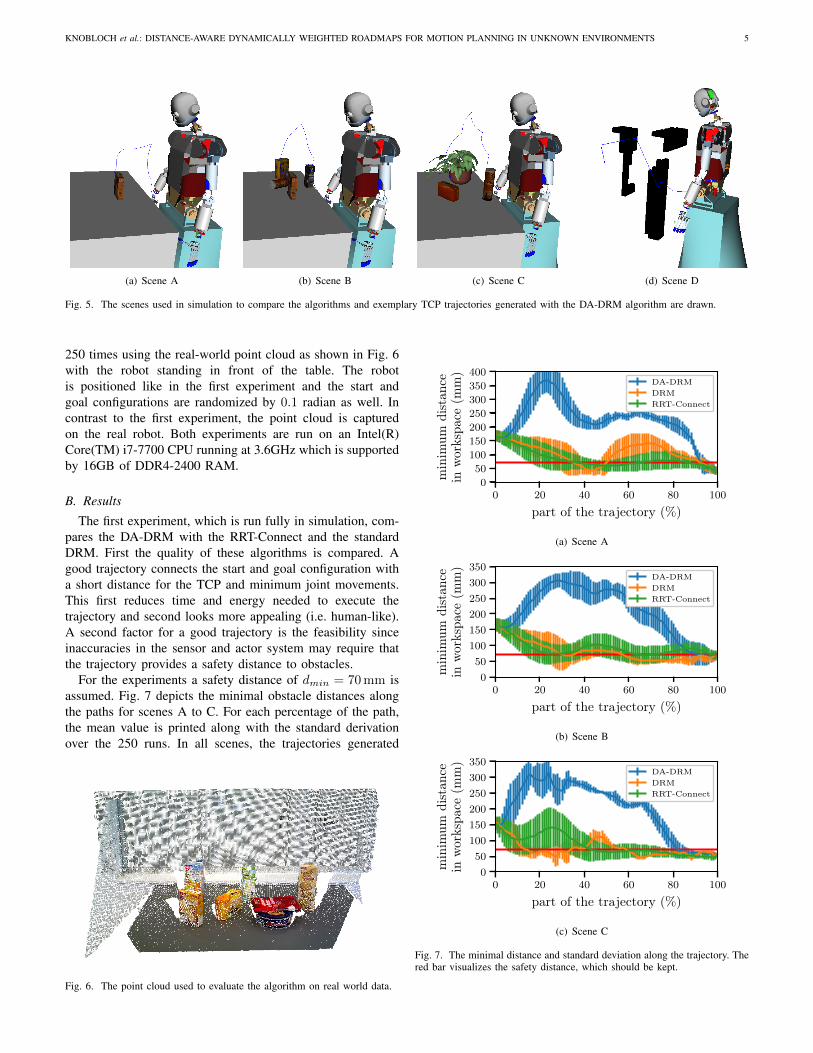
Fig. 5. The scenes used in simulation to compare the algorithms and exemplary TCP trajectories generated with the DA-DRM algorithm are drawn.

250 times using the real-world point cloud as shown in Fig. 6with the robot standing in front of the table. The robotis positioned like in the first experiment and the start andgoal configurations are randomized by 0.1 radian as well. Incontrast to the first experiment, the point cloud is capturedon the real robot. Both experiments are run on an Intel(R)Core(TM) i7-7700 CPU running at 3.6GHz which is supportedby 16GB of DDR4-2400 RAM.

B. Results

The first experiment, which is run fully in simulation, com-pares the DA-DRM with the RRT-Connect and the standardDRM. First the quality of these algorithms is compared. Agood trajectory connects the start and goal configuration witha short distance for the TCP and minimum joint movements.This first reduces time and energy needed to execute thetrajectory and second looks more appealing (i.e. human-like).A second factor for a good trajectory is the feasibility sinceinaccuracies in the sensor and actor system may require thatthe trajectory provides a safety distance to obstacles.

For the experiments a safety distance of dmin = 70mm isassumed. Fig. 7 depicts the minimal obstacle distances alongthe paths for scenes A to C. For each percentage of the path,the mean value is printed along with the standard derivationover the 250 runs. In all scenes, the trajectories generated

Fig. 6. The point cloud used to evaluate the algorithm on real world data.

0 20 40 60 80 100

part of the trajectory (%)

0

50

100

150

200

250

300

350

400

min

imum

dist

ance

inw

orks

pace

(mm

)

DA-DRMDRMRRT-Connect

(a) Scene A

0 20 40 60 80 100

part of the trajectory (%)

0

50

100

150

200

250

300

350

min

imum

dist

ance

inw

orks

pace

(mm

)

DA-DRMDRMRRT-Connect

(b) Scene B

0 20 40 60 80 100

part of the trajectory (%)

0

50

100

150

200

250

300

350

min

imum

dist

ance

inw

orks

pace

(mm

)

DA-DRMDRMRRT-Connect

(c) Scene C

Fig. 7. The minimal distance and standard deviation along the trajectory. Thered bar visualizes the safety distance, which should be kept.

6 IEEE ROBOTICS AND AUTOMATION LETTERS. PREPRINT VERSION. ACCEPTED JANUARY, 2018

Algorithm failed minimal averageDA-DRM 1.6 % 3.00mm 108.20mmDRM 0.4 % 0.003mm 28.81mmDRM 70mm 54.8 % 70.43mm 107.81mmRRT-Connect 5.6 % 0.001mm 36.25mmRRT-Connect 70mm 81.2 % 70.45mm 143.70mm

Fig. 8. The minimal distances to the environment evaluated for Scene D(5(d)). For each algorithm the number of failed runs, the minimal and averagedistance calculated over all runs is shown.

by the RRT-Connect and the DRM fall considerably belowthe safety distance. This is an expected result, because bothalgorithms do not include the safety distance in the calculation.In contrast to that, the DA-DRM keeps the safety distance forthe whole trajectory and violate this distance in the area closeto the goal configuration where the distance should fall belowsuch as distance to achieve the target.

The results for scene D are shown in (Fig. 8). While theRRT-Connect and the DRM again violate the safety distance,their equivalents, which consider the safety distance as blockedarea, always keep the safety distance. However, these algo-rithms have the highest number of failures, since they are notable to plan in narrow passages. The DA-DRM is always ableto plan a path in the given time if the adapted roadmap includesa path and follows the safety distance if possible. Thus sceneD shows, that the DA-DRM provides a good trade-off betweensuccessfully planning a path and ensuring the safety distance.

The smoothness of the trajectories is measured by thedistances in workspace and C-space, which are shown inFig. 9(a) and Fig. 9(b). The data is provided in a violinplot, where on the y-axis for each length the probabilitydensity is shown. On the x-axis the results are labeled by thescene number and the algorithm, while the results are sortedby the algorithm. These two diagrams show that the RRT-Connect provides the shortest trajectories in the C-space anddistances which are mostly equal to the other algorithms in theworkspace. The reason for this is the post-processing algorithmwhich optimizes for the shortest possible trajectory. For theDA-DRM, Fig. 9(a) shows, that it provides comparativelylong trajectories, which is affected by the safety distance. Forthe C-space, the results are different, as shown in Fig.9(b).The DA-DRM and the DRM algorithm generate trajectoriesof nearly equal length. This shows, that the DA-DRM algo-rithm provides smoother trajectories than the DRM algorithm,because trajectories of the DA-DRM algorithm allow moremovement in the workspace with similar joint movement. Butthese trajectories are not as smooth as those generated by theRRT-Connect, which again produces the shortest trajectories.Such short trajectories can not be generated by the DA-DRMsince it has to keep the safety distance.

The time needed to generate the trajectories is shown inFig. 10. The violin plot shows that the DRM takes with under100ms the least time. The DA-DRM algorithm needs 200msto 500ms in the mean which is about as much as the RRT-Connect needs. But in terms of consistency the DA-DRM beatsthe RRT-Connect. The RRT-Connect has much more variance

A B C D

0

500

1000

1500

2000

2500

3000

3500

leng

thin

wor

kspa

ce(m

m)

DA-DRM

A B C D

DRM

A B C D

Goalconfi

guration

incollision

Goalconfi

guration

incollision

Goalconfi

guration

incollision

DRM70mm

A B C D

RRT-Connect

A B C D

Goalconfi

guration

incollision

Goalconfi

guration

incollision

Goalconfi

guration

incollision

RRT-Connect70mm

(a) Trajectory length in workspace.

A B C D

0

5

10

15

20

leng

thin

c-Sp

ace

DA-DRM

A B C D

DRM

A B C D

Goalconfi

guration

incollision

Goalconfi

guration

incollision

Goalconfi

guration

incollision

DRM70mm

A B C D

RRT-Connect

A B C D

Goalconfi

guration

incollision

Goalconfi

guration

incollision

Goalconfi

guration

incollision

RRT-Connect70mm

(b) Trajectory length in C-space.

Fig. 9. The length of the trajectory in the workspace (9(a)) and C-space (9(b))for the different algorithms in the different scenes.

in the calculation time for each scene and has a high amountof runs which need about 1000ms in Scene D.

To understand the increase in duration for the DA-DRMagainst the DRM, we need to have a closer look at the durationof each step during the execution. For this purpose, the time fortrajectory generation using a real world point cloud is brokendown, in the second experiment. Fig. 11 depicts the durationof each step of the algorithm in a violin plot. As can be seen,the sum of the average duration is about 230ms, which is thetime needed in simulation.

The algorithm is divided into five major steps, while allother calculations need less than 5ms. First, the generate dis-tance grid step needs about 30ms. During this step, all pointsof the point cloud are iterated and the corresponding voxels aremarked. This includes the iteration over the adjacent voxels,whose number increases cubically with the safety distance.The cubical increase of the considered voxels is the reasonfor the relative high time consumption. The second step, whichneeds about 50ms is the adapt the graph step. During this stepall marked voxels are iterated and the corresponding nodes andedges are updated. Since the number of marked voxels is high

KNOBLOCH et al.: DISTANCE-AWARE DYNAMICALLY WEIGHTED ROADMAPS FOR MOTION PLANNING IN UNKNOWN ENVIRONMENTS 7

A B C D

0

200

400

600

800

1000

tim

e(m

s)

DA-DRM

A B C D

DRM

A B C D

Goalconfi

guration

incollision

Goalconfi

guration

incollision

Goalconfi

guration

incollision

DRM70mm

A B C D

RRT-Connect

A B C D

Goalconfi

guration

incollision

Goalconfi

guration

incollision

Goalconfi

guration

incollision

RRT-Connect70mm

Fig. 10. The calculation times for the different algorithms in the differentscenes.

generate distance gridadapt the graph

connect start and goalgraph search

post-processing

20

40

60

80

100

120

140

tim

e(m

s)

Fig. 11. The calculation time for each step of the DA-DRM using a realworld point cloud.

for large safety distances, this step needs a significant amountof time. In the third connect start and goal step, which needsabout 15ms, the start and goal configurations are connected tothe graph. This includes a k-nearest neighbors search, which issimply done by iterating over all nodes. It could be sped up byusing a cover-tree data structure ([18], [22]). The fourth step isthe graph search step, which only includes one run of the A?

algorithm. The duration of about 35 to 130ms is a result of thechanges of the edge weights. Because the weights are changed,the optimal path leads not along an edge created by the blockedpart of the environment, which increases the search area ofthe A? algorithm. Therefore, the number of nodes consideredduring a run is highly increased. In the last step, the graphis smoothed during the post-processing, which needs between40 and 120ms. To do this, new edges are created, which arenot included in the graph. Since the resulting trajectory has tobe self collision free, every new edge needs to be checked forself collisions, which is computationally costly.

C. DA-DRM Roadmap Parameter Evaluation

A DA-DRM roadmap has mainly three different parametersto adjust. These are the voxel size, the number of nodesand the number of edges per node. To find the best values,different roadmaps are calculated and then evaluated using the

test methods listed in the introduction of this section. As aninitial setup for the parameters, the values presented by Kunzet al. [18] are used. They use 16384 nodes, 20 edges per nodeand a voxel edge length of 50mm.

For the voxel size, smaller is theoretically better, since thisimproves the accuracy for the planning. To find a good voxelsize, roadmaps with 50mm, 40mm and 30mm voxel edgelength, each with 16384 nodes and 20 edges per node arecompared. While C-space and workspace length of the gen-erated trajectories do not differ much, the trajectory creationtime and the roadmap creation time are getting longer and theroadmap size is getting larger for smaller voxel edge lengths:

Voxel edge length (mm) 50 40 30Trajectory creation (ms) 100-150 100-230 150-250Roadmap creation (h:m) 3:38 7:10 18:10Roadmap size (MB) 859 1386 2637

For a voxel edge length of 50mm and 40mm the trajectorycreation time is very equal, with both under 200ms. The timefor roadmap creation with 30mm voxel edge length is muchhigher, because the number of adjacent voxel increases tocover the safety distance. In addition to the larger trajectorycreation time, the roadmap with 30mm voxel edge lengthneeds more than double the space and time to create theroadmap. The creation time of about 7 hours and the size of 1.3GB is reasonable for a roadmap. So using a voxel edge lengthof 40mm gives an improvement in accuracy with reasonablecreation time and space need.

Using a roadmap with more edges tends to generatesmoother trajectories, while the roadmap creation time, sizeand the trajectory generation time are increased. A roadmapwith 20 edges per node, as used by Kunz et al. [18], providesgood results for the DRM algorithm, while space and time re-quirements are reasonable, as shown above. For the DA-DRMalgorithm, 20 edges per node seems to be a good choice, whileless edges provide also reasonable results:

Edges per node 20 15Trajectory creation (ms) 100-230 100-240workspace length 1200-2400 1750-3000C-space length 8-15 9-17

The number of nodes affects the precision of the trajectoryplanning in different environments. More nodes increase theprobability, that a node is near to the goal configuration. Butan increase of nodes also increases the runtime of the A?, thepre-calculation time and the roadmap size. Since the numberof 16384 nodes provides a good precision, this number ofnodes is used throughout this work.

V. CONCLUSIONS

In this work, the DA-DRM algorithm is presented, whichextends the DRM algorithm by incorporating the distance toobstacles for trajectory generation. The obstacle distance of theplanned trajectories has been increased to maintain a safetydistance while achieving good performance. The DA-DRMalgorithm includes a post-processing step, which uses a createddistance grid to smooth the generated trajectories resulting in

8 IEEE ROBOTICS AND AUTOMATION LETTERS. PREPRINT VERSION. ACCEPTED JANUARY, 2018

shorter trajectories. In our evaluation scenarios, the runtime ofthe algorithm has been measured with values below 500mswhich makes it suitable for real-time applications. We alsoshowed that the algorithm is capable to deal with direct visualinput (i.e. point clouds) without the need of any computervision algorithms such as object detection and localization.

To improve the trajectory creation time, the algorithmcould be implemented using a field-programmable gate array(FPGA) as this was done for the DRM by Murray et al. [10].Since all extensions are working with the voxel grid and theW-C mapping, the adaptations to an implementation on theFPGA are easy to conduct.

REFERENCES

[1] S. M. LaValle, “Rapidly-exploring random trees: A new tool for pathplanning,” 1998.

[2] L. E. Kavraki, P. Svestka, J.-C. Latombe, and M. H. Overmars, “Prob-abilistic roadmaps for path planning in high-dimensional configurationspaces,” IEEE transactions on Robotics and Automation, vol. 12, no. 4,pp. 566–580, 1996.

[3] J. P. Van Den Berg and M. H. Overmars, “Roadmap-based motionplanning in dynamic environments,” IEEE Transactions on Robotics,vol. 21, no. 5, pp. 885–897, 2005.

[4] P. Leven and S. Hutchinson, “Toward real-time path planning inchanging environments,” in Workshop on Algorithmic Foundations ofRobotics., 2000.

[5] ——, “A framework for real-time path planning in changing environ-ments,” The International Journal of Robotics Research, vol. 21, no. 12,pp. 999–1030, 2002.

[6] M. Kallmann and M. Mataric, “Motion planning using dynamicroadmaps,” in Robotics and Automation, 2004. Proceedings. ICRA’04.2004 IEEE International Conference on, vol. 5. IEEE, 2004, pp. 4399–4404.

[7] H. Liu, X. Deng, H. Zha, and D. Ding, “A path planner in changingenvironments by using wc nodes mapping coupled with lazy edges eval-uation,” in Intelligent Robots and Systems, 2006 IEEE/RSJ InternationalConference on. IEEE, 2006, pp. 4078–4083.

[8] L. Jaillet and T. Simeon, “A PRM-based motion planner for dynamicallychanging environments,” in Intelligent Robots and Systems, 2004.(IROS2004). Proceedings. 2004 IEEE/RSJ International Conference on, vol. 2.IEEE, 2004, pp. 1606–1611.

[9] H. Akbaripour and E. Masehian, “Semi-lazy probabilistic roadmap: aparameter-tuned, resilient and robust path planning method for manip-ulator robots,” The International Journal of Advanced ManufacturingTechnology, pp. 1–30, 2016.

[10] S. Murray, W. Floyd-Jones, Y. Qi, D. Sorin, and G. Konidaris, “Robotmotion planning on a chip,” in Robotics: Science and Systems, 2016.

[11] Y. Yang, W. Merkt, V. Ivan, Z. Li, and S. Vijayakumar, “HDRM: Aresolution complete dynamic roadmap for real-time motion planning incomplex scenes,” 2017.

[12] Y. Yang, V. Ivan, Z. Li, M. Fallon, and S. Vijayakumar, “idrm:Humanoid motion planning with realtime end-pose selection in complexenvironments,” in Humanoid Robots (Humanoids), 2016 IEEE-RAS 16thInternational Conference on. IEEE, 2016, pp. 271–278.

[13] A. Voelz and K. Graichen, “Distance metrics for path planning withdynamic roadmaps,” in ISR 2016: 47st International Symposium onRobotics; Proceedings of. VDE, 2016, pp. 1–7.

[14] R. Geraerts and M. H. Overmars, “Creating high-quality paths formotion planning,” The International Journal of Robotics Research,vol. 26, no. 8, pp. 845–863, 2007.

[15] R. Diankov, “Automated construction of robotics manipulation pro-grams,” Ph.D. dissertation, Robotics Institute, Carnegie Mellon Univer-sity, 2010.

[16] S. Quinlan and O. Khatib, “Elastic bands: Connecting path planning andcontrol,” in Robotics and Automation, 1993. Proceedings., 1993 IEEEInternational Conference on. IEEE, 1993, pp. 802–807.

[17] N. Ratliff, M. Zucker, J. A. Bagnell, and S. Srinivasa, “CHOMP: Gradi-ent optimization techniques for efficient motion planning,” in Roboticsand Automation, 2009. ICRA’09. IEEE International Conference on.IEEE, 2009, pp. 489–494.

[18] T. Kunz, U. Reiser, M. Stilman, and A. Verl, “Real-time path planningfor a robot arm in changing environments,” in Intelligent Robots andSystems (IROS), 2010 IEEE/RSJ International Conference on. IEEE,2010, pp. 5906–5911.

[19] T. Asfour, K. Regenstein, P. Azad, J. Schroder, N. Vahrenkamp, andR. Dillmann, “ARMAR-III: An Integrated Humanoid Platform forSensory-Motor Control,” in IEEE/RAS International Conference onHumanoid Robots (Humanoids), Genova, Italy, December 2006, pp.169–175.

[20] N. Vahrenkamp, M. Wachter, M. Krohnert, K. Welke, and T. Asfour,“The robot software framework armarx,” it-Information Technology,vol. 57, no. 2, pp. 99–111, 2015.

[21] J. J. Kuffner and S. M. LaValle, “RRT-connect: An efficient approachto single-query path planning,” in Proceedings 2000 ICRA. MillenniumConference. IEEE International Conference on Robotics and Automa-tion. Symposia Proceedings (Cat. No.00CH37065), vol. 2, 2000, pp.995–1001.

[22] A. Beygelzimer, S. Kakade, and J. Langford, “Cover trees for nearestneighbor,” in Proceedings of the 23rd international conference onMachine learning. ACM, 2006, pp. 97–104.