IEEE TRANSACTION ON COMPUTATIONAL IMAGING, VOL. , NO. , XXXX 1

Low rank plus sparse decomposition ofsynthetic aperture radar data for target imaging

Matan Leibovich, George Papanicolaou, and Chrysoula Tsogka

Abstract—We analyze synthetic aperture radar (SAR)imaging of complex ground scenes that contain both sta-tionary and moving targets. In the usual SAR acquisitionscheme, we consider ways to preprocess the data so as toseparate the contributions of the moving targets from thosedue to stationary background reflectors. Both componentsof the data, that is, reflections from stationary and movingtargets, are considered as signal that is needed for targetimaging and tracking, respectively. The approach we useis to decompose the data matrix into a low rank and asparse part. This decomposition enables us to capture thereflections from moving targets into the sparse part andthose from stationary targets into the low rank part of thedata. The computational tool for this is robust principalcomponent analysis (RPCA) applied to the SAR data ma-trix. We also introduce a lossless baseband transformationof the data, which simplifies the analysis and improves theperformance of the RPCA algorithm. A modified versionof RPCA, the stable principal component pursuit (PCP),is robust to additive noise. Our main contribution is atheoretical analysis that determines an optimal choice ofparameters for the RPCA algorithm so as to have aneffective and stable separation of SAR data coming frommoving and stationary targets. This analysis gives also alower bound for detectable target velocities. We show inparticular that the rank of the sparse matrix is proportionalto the square root of the target’s speed in the directionthat connects the SAR platform trajectory to the imagingregion. The robustness of the approach is illustrated withnumerical simulations in the X-band SAR regime.

I. INTRODUCTION

A. Synthetic aperture radar imaging

Synthetic aperture radar can provide high resolu-tion imaging in several applications [1]. The SARdata are usually acquired by a moving platform thatprobes a remote area by sending broadband pulses,f(t), and recording the echoes. Although there is onlyone transmit-receive element, high resolution images are

M. Leibovich is with the Institute of Computational and Math-ematical Engineering, Stanford University, Stanford, CA E-mail:matanle@stanford.edu.

G. Papanicolaou is with the Department of Mathematics, StanfordUniversity, Stanford, CA E-mail: papanicolaou@stanford.edu

C. Tsogka is with the Department of Applied Mathematics, Univer-sity of California, Merced, 5200 North Lake Road, Merced, CA 95343E-mail:ctsogka@ucmerced.edu

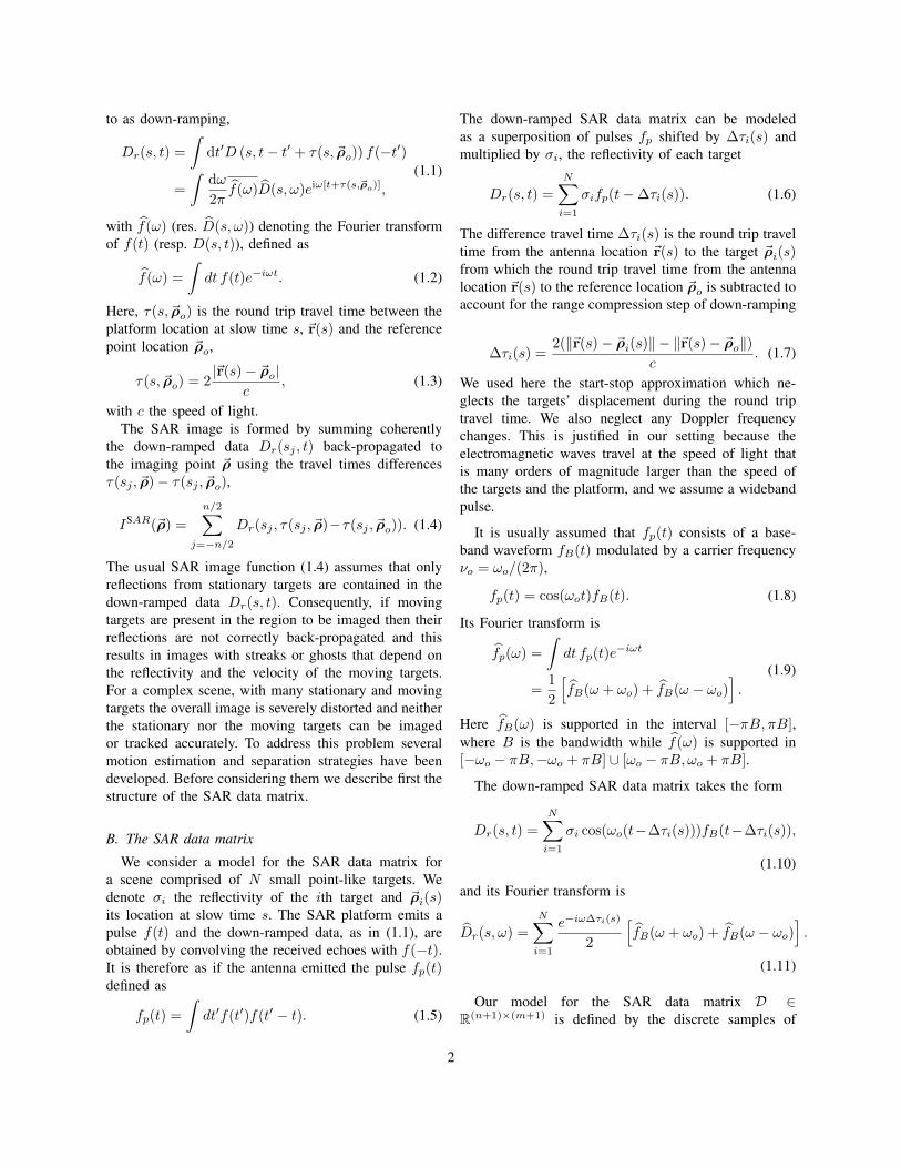
obtained by coherently processing the data collected bythe moving platform along a large synthetic aperture.Let ~r(s) denote the platform location at time s, calledthe slow time. The data collected form a matrix D(s, t),which records the echoes received at ~r(s) when a pulseis emitted from the same location. We consider n+1 dis-crete slow times with sampling interval ∆s, sj = j∆s,with j = −n/2, · · · , n/2. The fast time, t ∈ (0,∆s)runs between successive pulse emissions. A schematicof a SAR imaging configuration is shown in Figure 1.

f(t)

time ∆sD(s, t)

~r(s)

~ρ

Fig. 1: Synthetic aperture imaging schematic.

To maximize the power delivered to the region to beimaged, the probing signals used in SAR are long pulsesof support tc � 1/B where B denotes the bandwidthof the probing pulse. An example of such signals arelinear frequency modulated chirps [1]. To concentrate theenergy of the reflected echoes to a small time intervalof size 1/B the received signal is convolved with thetime-reversed emitted pulse. This step is called pulsecompression and is followed by a range compressionstep which consists of migrating the pulse compresseddata to a reference point ~ρo in the imaging window. Therange-compression step removes from the data the largephase ωτ(s, ~ρo). These two steps together are referred

to as down-ramping,

Dr(s, t) =

∫dt′D (s, t− t′ + τ(s, ~ρo)) f(−t′)

=

∫dω

2πf(ω)D(s, ω)eiω[t+τ(s,~ρo)],

(1.1)

with f(ω) (res. D(s, ω)) denoting the Fourier transformof f(t) (resp. D(s, t)), defined as

f(ω) =

∫dt f(t)e−iωt. (1.2)

Here, τ(s, ~ρo) is the round trip travel time between theplatform location at slow time s, ~r(s) and the referencepoint location ~ρo,

τ(s, ~ρo) = 2|~r(s)− ~ρo|

c, (1.3)

with c the speed of light.The SAR image is formed by summing coherently

the down-ramped data Dr(sj , t) back-propagated tothe imaging point ~ρ using the travel times differencesτ(sj , ~ρ)− τ(sj , ~ρo),

ISAR(~ρ) =

n/2∑j=−n/2

Dr(sj , τ(sj , ~ρ)−τ(sj , ~ρo)). (1.4)

The usual SAR image function (1.4) assumes that onlyreflections from stationary targets are contained in thedown-ramped data Dr(s, t). Consequently, if movingtargets are present in the region to be imaged then theirreflections are not correctly back-propagated and thisresults in images with streaks or ghosts that depend onthe reflectivity and the velocity of the moving targets.For a complex scene, with many stationary and movingtargets the overall image is severely distorted and neitherthe stationary nor the moving targets can be imagedor tracked accurately. To address this problem severalmotion estimation and separation strategies have beendeveloped. Before considering them we describe first thestructure of the SAR data matrix.

B. The SAR data matrix

We consider a model for the SAR data matrix fora scene comprised of N small point-like targets. Wedenote σi the reflectivity of the ith target and ~ρi(s)its location at slow time s. The SAR platform emits apulse f(t) and the down-ramped data, as in (1.1), areobtained by convolving the received echoes with f(−t).It is therefore as if the antenna emitted the pulse fp(t)defined as

fp(t) =

∫dt′f(t′)f(t′ − t). (1.5)

The down-ramped SAR data matrix can be modeledas a superposition of pulses fp shifted by ∆τi(s) andmultiplied by σi, the reflectivity of each target

Dr(s, t) =

N∑i=1

σifp(t−∆τi(s)). (1.6)

The difference travel time ∆τi(s) is the round trip traveltime from the antenna location ~r(s) to the target ~ρi(s)from which the round trip travel time from the antennalocation ~r(s) to the reference location ~ρo is subtracted toaccount for the range compression step of down-ramping

∆τi(s) =2(‖~r(s)− ~ρi(s)‖ − ‖~r(s)− ~ρo‖)

c. (1.7)

We used here the start-stop approximation which ne-glects the targets’ displacement during the round triptravel time. We also neglect any Doppler frequencychanges. This is justified in our setting because theelectromagnetic waves travel at the speed of light thatis many orders of magnitude larger than the speed ofthe targets and the platform, and we assume a widebandpulse.

It is usually assumed that fp(t) consists of a base-band waveform fB(t) modulated by a carrier frequencyνo = ωo/(2π),

fp(t) = cos(ωot)fB(t). (1.8)

Its Fourier transform is

fp(ω) =

∫dt fp(t)e

−iωt

=1

2

[fB(ω + ωo) + fB(ω − ωo)

].

(1.9)

Here fB(ω) is supported in the interval [−πB, πB],where B is the bandwidth while f(ω) is supported in[−ωo − πB,−ωo + πB] ∪ [ωo − πB, ωo + πB].

The down-ramped SAR data matrix takes the form

Dr(s, t) =

N∑i=1

σi cos(ωo(t−∆τi(s)))fB(t−∆τi(s)),

(1.10)

and its Fourier transform is

Dr(s, ω) =

N∑i=1

e−iω∆τi(s)

2

[fB(ω + ωo) + fB(ω − ωo)

].

(1.11)

Our model for the SAR data matrix D ∈R(n+1)×(m+1) is defined by the discrete samples of

2

(1.10),

Dil = Dr

(si−n2−1, tl−1

),

i = 1, . . . , n+ 1, l = 1, . . . ,m+ 1,(1.12)

with slow times sj defined by

sj = j∆s, j = −n/2, . . . , n/2, (1.13)

and fast times tl defined as

tl = l∆t, l = 1, . . . ,m. (1.14)

Here we assumed that ∆s is an integer multiple of ∆tand set m = ∆s/∆t.

C. Motion estimation and separation strategies

A simple way to separate moving targets from the sta-tionary background is the change detection (CD) method.In video surveillance, this amounts to subtracting thedata corresponding to two consecutive frames. Assumingthat multi-frame SAR images, which show the samescene at different times, are available, CD can be usedin SAR. We refer to [2] where CD is used for detectingmoving targets in multi-frame SAR imagery and to [3]where CD was implemented for human motion trackingwith through-the-wall radar. A similar method is theCoherent Change Detection (CCD) which also involvesperforming repeat pass radar data collection. However,the change detection part is now different. Change isdetected in CCD by identifying zeros in the cross-correlation between pairs of images [4], [5], [6].

A specific form of CD that has been used extensivelyin SAR is the Displaced Phase Center Antenna (DPCA)method, in which the platform uses two antennas, syn-chronized so that the second antenna is following thesame trajectory as the first with a certain time delay.Subtracting the two traces eliminates the stationary back-ground echoes, leaving only the echoes from movingtargets [7], [1]

Another method that has been used for moving tar-get detection is autofocus [8], [9], [10], [11]. Thesealgorithms exploit the fact that target motion introducesphase errors, which result in smearing of the target’simage. Autofocus algorithms can be used in the classicalsingle channel SAR setup, and they have two steps: firstthe conventional smeared images are formed followed bya phase error estimation and compensation of the imageparts that correspond to moving targets.

A lot of progress has also been achieved in space-time adaptive processing algorithms which aim to betterdetect the moving targets by suppressing the ”clutter”of stationary targets. Examples are the multi-channelSAR [12], the space-time-frequency SAR [13], velocity

SAR (VSAR) [14] and dual-speed SAR [15]. Morerecently compressed sensing and sparsity driven methodsmade their way into the moving target SAR imagingproblem [16]. We refer the reader to [17] for a reviewon sparsity driven synthetic aperture imaging includingmoving target imaging.

D. Robust principal component analysis

RPCA has been extensively used in SAR in variousapplications. In [18], [19] for example, a multi channelapproach was used. By combining the different channels,the background forms, ideally, a low rank matrix. In[20] the 2D-SAR data are stacked to form a longvector and RPCA is used to decompose this vector intothree parts: clutter, moving targets and noise using adictionary representation for both the moving and thestationary parts. Other works, as [21], [22], utilize low-rank and sparsity assumptions in the formed image andsparsity is imposed using priors and a sparse dictionaryrepresentation.

We follow here the approach proposed and analyzedin [23], where the robust principal component algorithmwas used for separating the data matrix D in (1.12) intotwo subsets: the echoes due to stationary targets thatnormally form the low rank part of the data matrix andthose due to moving targets echoes which constitute thesparse part. The RPCA method consists of solving thefollowing convex optimization problem,

minL,S∈Rn1×n2 ||L||∗ + η||S||1 (1.15)subject to L+ S = D. (1.16)

Here ||L||∗ denotes the nuclear norm, that is the sumof the singular values of L, and ||S||1 is the matrix`1-norm of S. Assuming the matrix D ∈ Rn1×n2 isthe sum of a low rank matrix Lo and a sparse matrixSo then the solution of the optimization (1.15)-(1.16)recovers Lo and So exactly, under sufficient conditions.This optimization problem has been analyzed in [24],where sufficient conditions for the decomposition to beexact are derived.

RPCA is well suited for target separation in SARdata, since we expect the echoes from the backgroundand the moving target to form a low-rank and a sparsematrix, respectively. Indeed, with apertures over sta-tionary scenes, reflections from the background will bevarying mostly due the platform’s movement, whichis largely compensated for by range compression. Onthe other hand, reflections from moving targets havelocalized support, positioned at different locations forevery slow time, due to the target’s motion. Within the

3

point scatterer model, this difference is manifested byd∆τ(s)ds being much smaller for stationary targets than

for moving ones. Moreover, as shown in Section III-A,in the context of RPCA, low-rankness can be quantifiedby the ratio of the nuclear and the `1 norms. This ratio,which is smaller for a stationary target compared to amoving one, is expected to remain essentially the sameas the complexity of the background increases.

The parameter η that balances the ratio between thenuclear norm of L and the `1-norm of S plays animportant role in our analysis. The main idea is thatwe want to chose the value of η given that L and S soas to represent the echoes received from stationary andmoving targets. The recommended value for η proposedin [24] and used for SAR data in [23] is

η =1√

max{n1, n2}. (1.17)

It was shown in [23] that, with this choice of η, theRPCA algorithm is sensitive to the window size of thedata. Moreover, for complex scenes successful separationbetween moving and stationary targets’ echoes can beachieved only with adequate windowing of the SAR data.

RPCA assumes that the matrix D is comprised ofsolely a low rank part and a sparse part. In the presenceof additive noise, characterized by a parameter δ, amodified algorithm, stable PCP [25], can be used. Itsolves the convex problem

minL,S∈Rn1×n2 ||L||∗ + η||S||1 (1.18)subject to ‖L+ S − D‖F ≤ δ (1.19)

η plays the same role in stable PCP. An example ispresented in Figure 2d.

E. Summary of main results

We determine in this paper an optimal range for theparameter η, by taking into consideration the specificform that the L and S matrices take in the SAR problem.Specifically, by analytically computing the nuclear and`1 norms for a single stationary and moving target, weobtain a range of values for η for which robust separationresults can be obtained with RPCA. Furthermore, ouranalysis shows that the range of acceptable values for ηincreases with increasing velocity of the moving target.This is expected since for increasing target velocity theechoes from the moving target become more sparseor equivalently less low rank. Thus, they can be moreeasily separated from the stationary targets’ echoes. Thisimplies in particular that targets that are moving with aspeed above a certain threshold can be easily detected.More precisely, it is the projection of the velocity along

the direction that connects the SAR platform to the imag-ing domain that matters. This is because for targets thatare moving parallel to that direction, smaller variation intravel times is expected.

Our analysis suggests that the RPCA algorithm shouldbe applied on the baseband data matrix DB which isobtained from the down-ramped data, D, using a losslesstransformation that consists of shifting the signal in thefrequency domain so that it is centered at ω = 0 insteadof ω = ωo. Going to baseband allows us to evaluatethe performance of the RPCA algorithm for a widerrange of moving target speeds. This transformation alsoimproves the accuracy of our theoretical analysis andour numerical results indicate that it also improves therobustness of RPCA.

We derive a closed form expression for an optimalvalue of the RPCA parameter, η∗, for both the basebandand the original SAR data matrix. We show that usingη∗ does yield results that are more robust, especially forthe baseband case. Robustness is observed with respectto the window size of the SAR data, the complexity ofthe scene and the moving target’s velocity.

Numerical simulations carried out in a widebandregime for X-band surveillance SAR are in very goodagreement with our analytical results. In particular, weshow results with multiple, stationary point reflectors, anextended reflector, and SAR data with additive noise.

II. ROBUST PCA FOR MOTION DETECTION AND SARDATA SEPARATION

We present here the robust PCA algorithm adapted tothe SAR problem. We first explain the baseband trans-formation. The performance of RPCA on the basebanddata matrix is theoretically equivalent to the one onthe original data matrix, but going to baseband greatlysimplifies the analysis. We also see numerically thatit yields more robust behavior, in a sense that will beexplained in the analysis section III.

A. Baseband data matrixThe proposed preprocessing takes the original data

matrix and creates a baseband (BB) version of it byperforming band pass filtering at every slow time s.

Assuming the model of (1.6) for a single scatterer, theFourier transform of the down-ramped data is

Dr(s, ω) =e−iω∆τ(s)

2

[fB(ω + ωo) + fB(ω − ωo)

].

Thus, the Fourier transform of Do(s, t) = eiωotDr(s, t)is

Do(s, ω) =e−i(ω−ωo)∆τ(s)

2

[fB(ω) + fB(ω − 2ωo)

].

4

We then filter out the signal centered around 2ωo to geta baseband signal centered around ω = 0,

DrB(s, ω) = hLP (ω)Do(s, ω) = e−i(ω−ωo)∆τ(s)fB(ω).

There is no intersection between the supports since weassume ωo � B (narrow band regime). Thus, the filtercan be e.g.,

hLP (ω) =

{2 |ω| ≤ 2πB

0 |ω| > α2πB,

where αB < 2νo − B is small enough to eliminate thesignal centered around 2ωo. The factor of 2 ensures themaximum absolute value remains 1.

In the time domain we will get a filtered signal of theform

DrB(s, t) = eiωo∆τ(s)fB(t−∆τ(s)). (2.20)

No data is lost in the process, and the original data matrixcan be reconstructed by taking the real part of the BBdata multiplied by e−iωot ,

Dr(s, t) = <{e−iωotDrB(s, t)

}.

We define DB, the baseband data matrix, by applyingthe Discrete Fourier Transform (DFT) to the data matrixD with respect to its columns, and applying a similardiscrete filter to go to baseband. Assuming a smallenough ∆t the DFT is a good approximation of theFourier transform and we have

(DB)il = DrB(si−n2−1, tl−1),

i = 1, . . . , n+ 1, l = 1, . . . ,m+ 1.(2.21)

B. Modification of RPCA for complex matrices

Following [26] we use the inexact augmented La-grangian implementation of RPCA as described in Al-gorithm 1. This algorithm iteratively approximates thesolution by alternatively minimizing the following aug-mented Lagrangian with respect to L and S

‖L‖∗ + η‖S‖1 + 〈Y,D − L− S〉+µ

2‖D − L − S‖2F ,

where 〈A,B〉 = tr(ATB) is the regular matrix norm.Each of the minimization steps has an analytical solutiongiven by either spectral- or element-wise thresholding.

The RPCA algorithm can be adapted for use on com-plex matrices by modifying the thresholding associatedwith `1 minimization to preserve the argument of thenumber,

Θη(a) = ei arg a max(|a| − η, 0). (2.22)

The penalty term coefficient increases with everyiteration, usually geometrically µk+1 = ρµk.

Algorithm 1 D = L + S Inexact ALM method (algo-rithm no. 5 in [26], see also for initial parameters’ choiceand update).

1: Input: Observation matrix D ∈ Cm×n

2: Y0 = D/J(D);So = 0;µ0 > 0; ρ > 1; k =

0 J(D) = max(‖D‖2, η−1‖D‖∞

)3: while not converged do4: [Uk+1,Σk+1, Vk+1] = svd(D − Sk − µ−1

k Yk)

5: Lk+1 = Uk+1Θµ−1k

[Σk+1]V ∗k+1

6: Sk+1 = Θηµ−1k

[D − Lk+1 + µ−1k Yk]

7: Yk+1 = Yk + µk(D − Lk+1 − Sk+1)

8: µk+1 = ρµk

9: k → k + 1

10: end while11: return Lk+1,Sk+1

Based on [26], initial parameters were set to µ0 =1.2/‖D‖2 and ρ = 1.4.

For stable PCP, we put an upper bound on µ that isproportional to the noise level. Assuming a weak movingscatterer, the noise affects the S part, and so setting anupper bound on µ, µ ∝ η

σ(δ) , where σ is the varianceof the noise, results in effectively thresholding the noiseaway from the sparse part.

As shown in Figure 2d, the performance of stable PCPis comparable to that of RPCA.

C. Robustness of RPCA with optimal η

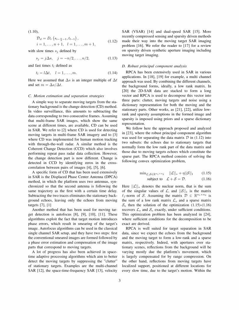
Before presenting our analysis, we illustrate with anumerical simulation the robustness of RPCA when theoptimal parameter η is used. The value for the optimalη is derived in Section III-A and is denoted η∗. Weconsider a scene with five stationary targets and onemoving target at a speed 15 m/s. The moving target’sreflectivity is 5% of the stationary targets’, which makesthe detection of the moving target quite challenging. Weshow the SAR data matrix and its L+S decompositionin Figure 2. The performance of RPCA with the con-ventional choice for η, i.e., η = 1√

max(n1,n2)is not very

good when applied to the entire data matrix (see Figure2a). The results are significantly improved when RPCAis applied after the data have been decomposed into 5consecutive windows in fast time as seen in Figure 2b.The plots in Figure 2c illustrate that RPCA achieves verygood separation without any data windowing when theoptimal parameter η∗ is used.

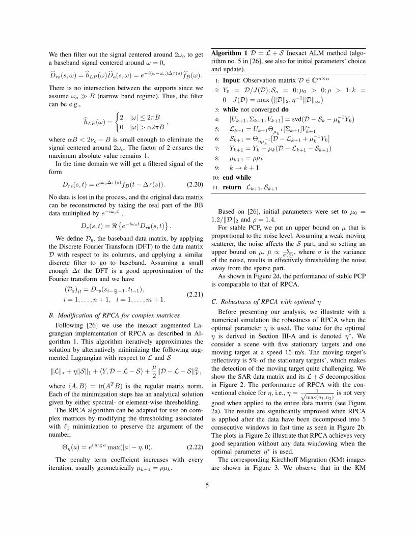
The corresponding Kirchhoff Migration (KM) imagesare shown in Figure 3. We observe that in the KM

5

(a) Original (left), low rank (middle) and sparse (right) partof the data obtained with RPCA using η = 1√

max(n1,n2)=

3.5× 10−3 . RPCA applied to the entire data matrix D (1window).

(b) Same as (a) but RPCA is applied after decomposing thedata into 5 consecutive windows in fast time, as suggested in[23].

(c) RPCA applied to the entire data matrix D using the optimalη∗ = 7.5× 10−3

(d) Stable PCP with with added white Gaussian noise N .SNR=10 log10

‖S‖2F‖N‖2

F= −5dB. Same η∗ is used as in 2c.

Fig. 2: Example of the performance of RPCA appliedto a scene with five stationary targets and one movingtarget with speed 15 m/s. The moving target’s reflectivityis 5% of the stationary targets’. This example illustratesthat very good L+ S separation can be achieved usinglarger windows when the optimal parameter η is used.We achieve similar results for stable PCP.

image of the original data matrix the moving target isnot detectable (see Figure 3a). We also see that a lotof clutter is present in the KM image of the sparsematrix generated by the conventional choice of η (seeFigure 3c). This is the result of stationary target’s energyleakage into the sparse part. The KM image of the sparsematrix generated by the optimal choice of η is shownin Figure 3d. We observe a significant improvement inseparation compared to the results obtained with theconventional choice of η. As expected improvement inthe L+S separation implies increased clutter suppressionfor both the moving and the stationary targets’ images.

III. ANALYSIS OF RPCA FOR MOTION ESTIMATION

We carry out in this section the analysis of theRPCA algorithm for motion estimation. This will allowus to determine the optimal range of values for theparameter η.

A. RPCA behavior as a function of η

The conventional value for the parameter η is1√

max(n1,n2), where n1, n2 are the dimensions of the

data matrix to be analyzed (cf. [24]). This choice ismotivated by assuming that the sparse part is randomnoise, sparsely supported in the data matrix. However,this is not the case for the SAR data.

By taking into account the specific form of L andS for the SAR problem, we derive an optimal rangeof values for η. Our analysis is based on the followingobservation: The ability of RPCA to separate betweenstationary and moving targets is due to the differencein their corresponding matrix norms. The two necessaryconditions for the algorithm to achieve separation are:

‖A‖∗ < η‖A‖1, for all low rank matrices A, (3.23)

and

‖A‖∗ > η‖A‖1, for all sparse matrices A. (3.24)

These conditions suggest the following restrictions on η

η >‖A‖∗‖A‖1

, for all low rank matrices A,

η <‖A‖∗‖A‖1

, for all sparse matrices A.(3.25)

We can therefore define the following range of valuesfor η, ηmin ≤ η ≤ ηmax,

with ηmin = supA low rank

‖A‖∗‖A‖1

, ηmax = infA sparse

‖A‖∗‖A‖1

.

(3.26)

6

(a) Kirchhoff Migration applied to the origi-nal data matrix.

(b) KM applied to the low rank part.

(c) KM with exact motion estimation param-eters applied to the sparse matrix generatedby the conventional choice of η.

(d) KM with exact motion estimation param-eters applied to the sparse matrix generatedby the optimal choice of η.

Fig. 3: Imaging applied to RPCA-separated data ofFig. 2. We observe a significant improvement in the SNRwhen the optimal η is used in the L+S decomposition.

Note that (3.26) is a necessary condition but not suffi-cient. Thus, it provides only an estimate of the range ofallowed values for η. An optimal η can be determinedby minimizing an objective. For example,

minη

F (η) =ηmin

η+

η

ηmax

⇒ η∗ =√ηminηmax, F (η∗) = 2

√ηmin

ηmax.

(3.27)

This objective provides a value for η∗ that givesgood separation results for all the examples we haveconsidered. It can be modified to account for priorinformation, e.g. if the reflectivity of the moving scattereris very weak then we may chose a different objective thatprovides a higher value for η∗.

We note that our analysis implies that η is independentof any global matrix normalization, i.e. ‖λA‖∗‖λA‖1 = ‖A‖∗

‖A‖1 ,and, assuming that there is little variance in the norm ofthe rows of the SAR data matrix, η is independent ofany row normalization as well. We next analyze each ofthe terms, i.e., ηmin and ηmax to arrive at a closed formexpression for η∗. We then show that using this η∗ doesyield results that are more robust, meaning that there isno need for fine tuning the windowing of the SAR dataand L + S separation is achieved for a wider range ofmoving target’s velocities.

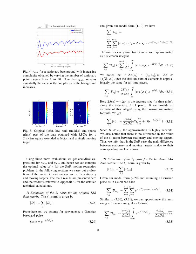
This observation also gives a quantitative estimatefor the concepts of ‘low-rank’ and ‘sparsity’ in thecontext of RPCA. A background would retain its ‘low-rankness’ as long as the ratio of the nuclear and `1norms is small enough. In Figure 4, we see that thegrowth rate of ηmin with the background’s complexityis very small, justifying the use of a single target inour analysis. Numerical simulations also suggest that thislow-rankness property remains true for extended objectsas seen in Figure 5.

To summarize, we see that the low-rank property ofthe stationary background is retained for RPCA evenas the scene becomes more complex, including multiplepoint scatterers or extended reflectors.

B. Estimation of matrix norms in the SAR model

We choose as a representative of each class of matri-ces, i.e. sparse and low rank, a data matrix for a singletarget, either stationary or moving. We then compute thecorresponding matrix norms in both cases and arrive atanalytical expressions for ηmin and ηmax as in (3.26).While this is a restricted class of cases, we show throughnumerical simulations that a single stationary target is agood representative of the class of stationary backgroundmatrices (see Figure 6).

7

Fig. 4: ηmin for a stationary background with increasingcomplexity obtained by varying the number of stationarypoint targets from 1 to 30. Note that ηmin remainsessentially the same as the complexity of the backgroundincreases.

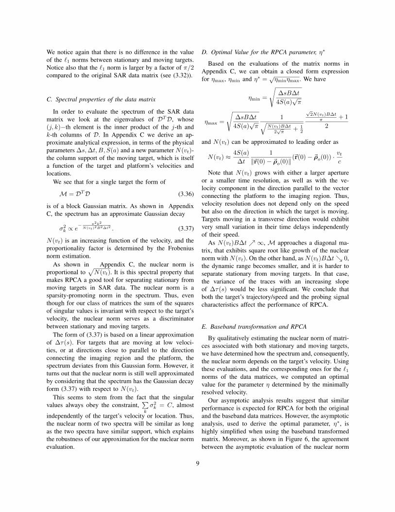
Fig. 5: Original (left), low rank (middle) and sparse(right) part of the data obtained with RPCA for a2m×2m square extended reflector, and a single movingtarget.

Using these norm evaluations we get analytical ex-pressions for ηmax and ηmin and hence we can computethe optimal value of η for the SAR motion separationproblem. In the following sections we carry out evalua-tions of the matrix `1 and nuclear norms for stationaryand moving targets. The main results are presented hereand the reader is referred to Appendix C for the detailedtechnical calculations.

1) Estimation of the `1 norm for the original SARdata matrix: The `1 norm is given by

‖D‖1 =∑i,j

|Dij |. (3.28)

From here on, we assume for convenience a Gaussianbaseband pulse

fB(t) = e−B2t2/2 (3.29)

and given our model form (1.10) we have∑i,j

|Dij | =

n+1∑i=1

m+1∑j=1

| cos(ωo(tj −∆τ(si))|e−B2(tj−∆τ(si))

2/2.

The sum for every time trace can be well approximatedas a Riemann integral,

∑i,j

|Dij | ≈n+1∑i=1

1

∆t

∞∫−∞

| cos(ωot)|e−B2t2/2dt. (3.30)

We notice that if ∆τ(si) ∈ [t0, tm],∀i, ∆t �{1/B, ωo}, then the absolute sum of elements is approx-imately the same for all time traces,

∑i,j

|Dij | ≈2S(a)

∆s∆t

∞∫−∞

| cos(ωot)|e−B2t2/2dt. (3.31)

Here 2S(a) = n∆s, is the aperture size (in time units),along the trajectory. In Appendix B we provide anestimate of this integral using the Poisson summationformula. We get∑

i,j

|Dij | ≈2S(a)

∆sB∆t2

√2

π+O(e−2ω2

o/B2

). (3.32)

Since B � ωo, the approximation is highly accurate.We also notice that there is no difference in the valueof the `1 norm between stationary and moving targets.Thus, we infer that, in the SAR case, the main differencebetween stationary and moving targets is due to theircorresponding nuclear norms.

2) Estimation of the `1 norm for the baseband SARdata matrix: The `1 norm is given by

‖DB‖1 =∑i,j

|DBij |. (3.33)

Given our model form (2.20) and assuming a Gaussianpulse as in (3.29) we have∑

i,j

|DBij | =n+1∑i=1

m+1∑j=1

e−B2(tj−∆τ(si))

2/2. (3.34)

Similar to (3.30), (3.31), we can approximate this sumusing a Riemann integral as follows,

∑i,j

|DBij | ≈2S(a)

∆s∆t

∞∫−∞

e−B2t2/2dt =

2S(a)

∆sB∆t

√2π.

(3.35)

8

We notice again that there is no difference in the valueof the `1 norms between stationary and moving targets.Notice also that the `1 norm is larger by a factor of π/2compared to the original SAR data matrix (see (3.32)).

C. Spectral properties of the data matrix

In order to evaluate the spectrum of the SAR datamatrix we look at the eigenvalues of DTD, whose(j, k)−th element is the inner product of the j-th andk-th columns of D. In Appendix C we derive an ap-proximate analytical expression, in terms of the physicalparameters ∆s,∆t, B, S(a) and a new parameter N(vt)-the column support of the moving target, which is itselfa function of the target and platform’s velocities andlocations.

We see that for a single target the form of

M = DTD (3.36)

is of a block Gaussian matrix. As shown in AppendixC, the spectrum has an approximate Gaussian decay

σ2k ∝ e

− π2k2

N(vt)2B2∆t2 . (3.37)

N(vt) is an increasing function of the velocity, and theproportionality factor is determined by the Frobeniusnorm estimation.

As shown in Appendix C, the nuclear norm isproportional to

√N(vt). It is this spectral property that

makes RPCA a good tool for separating stationary frommoving targets in SAR data. The nuclear norm is asparsity-promoting norm in the spectrum. Thus, eventhough for our class of matrices the sum of the squaresof singular values is invariant with respect to the target’svelocity, the nuclear norm serves as a discriminatorbetween stationary and moving targets.

The form of (3.37) is based on a linear approximationof ∆τ(s). For targets that are moving at low veloci-ties, or at directions close to parallel to the directionconnecting the imaging region and the platform, thespectrum deviates from this Gaussian form. However, itturns out that the nuclear norm is still well approximatedby considering that the spectrum has the Gaussian decayform (3.37) with respect to N(vt).

This seems to stem from the fact that the singularvalues always obey the constraint,

∑k

σ2k = C, almost

independently of the target’s velocity or location. Thus,the nuclear norm of two spectra will be similar as longas the two spectra have similar support, which explainsthe robustness of our approximation for the nuclear normevaluation.

D. Optimal Value for the RPCA parameter, η∗

Based on the evaluations of the matrix norms inAppendix C, we can obtain a closed form expressionfor ηmax, ηmin and η∗ =

√ηminηmax. We have

ηmin =

√∆sB∆t

4S(a)√π

ηmax =

√∆sB∆t

4S(a)√π

1√N(vt)B∆t

2√π

+ 12

√2N(vt)B∆t

π + 1

2

and N(vt) can be approximated to leading order as

N(vt) ≈4S(a)

∆t

1

‖~r(0)− ~ρo(0)‖(~r(0)− ~ρo(0)) · vt

c

Note that N(vt) grows with either a larger apertureor a smaller time resolution, as well as with the ve-locity component in the direction parallel to the vectorconnecting the platform to the imaging region. Thus,velocity resolution does not depend only on the speedbut also on the direction in which the target is moving.Targets moving in a transverse direction would exhibitvery small variation in their time delays independentlyof their speed.

As N(vt)B∆t ↗ ∞, M approaches a diagonal ma-trix, that exhibits square root like growth of the nuclearnorm with N(vt). On the other hand, as N(vt)B∆t↘ 0,the dynamic range becomes smaller, and it is harder toseparate stationary from moving targets. In that case,the variance of the traces with an increasing slopeof ∆τ(s) would be less significant. We conclude thatboth the target’s trajectory/speed and the probing signalcharacteristics affect the performance of RPCA.

E. Baseband transformation and RPCA

By qualitatively estimating the nuclear norm of matri-ces associated with both stationary and moving targets,we have determined how the spectrum and, consequently,the nuclear norm depends on the target’s velocity. Usingthese evaluations, and the corresponding ones for the `1norms of the data matrices, we computed an optimalvalue for the parameter η determined by the minimallyresolved velocity.

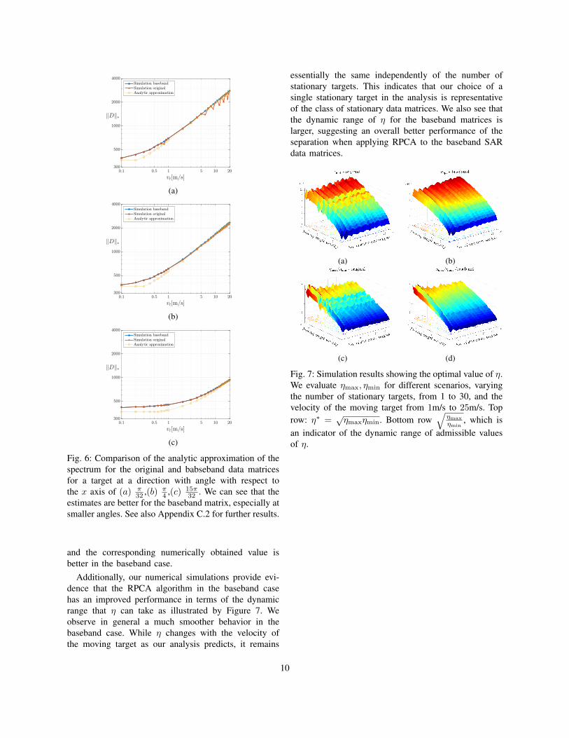
Our asymptotic analysis results suggest that similarperformance is expected for RPCA for both the originaland the baseband data matrices. However, the asymptoticanalysis, used to derive the optimal parameter, η∗, ishighly simplified when using the baseband transformedmatrix. Moreover, as shown in Figure 6, the agreementbetween the asymptotic evaluation of the nuclear norm

9

(a)

(b)

(c)

Fig. 6: Comparison of the analytic approximation of thespectrum for the original and babseband data matricesfor a target at a direction with angle with respect tothe x axis of (a) π

32 ,(b) π4 ,(c) 15π

32 . We can see that theestimates are better for the baseband matrix, especially atsmaller angles. See also Appendix C.2 for further results.

and the corresponding numerically obtained value isbetter in the baseband case.

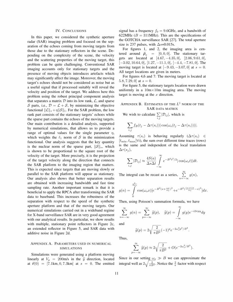
Additionally, our numerical simulations provide evi-dence that the RPCA algorithm in the baseband casehas an improved performance in terms of the dynamicrange that η can take as illustrated by Figure 7. Weobserve in general a much smoother behavior in thebaseband case. While η changes with the velocity ofthe moving target as our analysis predicts, it remains

essentially the same independently of the number ofstationary targets. This indicates that our choice of asingle stationary target in the analysis is representativeof the class of stationary data matrices. We also see thatthe dynamic range of η for the baseband matrices islarger, suggesting an overall better performance of theseparation when applying RPCA to the baseband SARdata matrices.

(a) (b)

(c) (d)

Fig. 7: Simulation results showing the optimal value of η.We evaluate ηmax, ηmin for different scenarios, varyingthe number of stationary targets, from 1 to 30, and thevelocity of the moving target from 1m/s to 25m/s. Toprow: η∗ =

√ηmaxηmin. Bottom row

√ηmax

ηmin, which is

an indicator of the dynamic range of admissible valuesof η.

10

IV. CONCLUSIONS

In this paper, we considered the synthetic apertureradar (SAR) imaging problem and focused on the sep-aration of the echoes coming from moving targets fromthose due to the stationary reflectors in the scene. De-pending on the complexity of the scene, the velocityand the scattering properties of the moving target, thisproblem can be quite challenging. Conventional SARimaging accounts only for stationary targets and thepresence of moving objects introduces artefacts whichmay significantly affect the image. Moreover, the movingtarget’s echoes should not be considered as noise but asa useful signal that if processed suitably will reveal thevelocity and position of the target. We address here thisproblem using the robust principal component analysisthat separates a matrix D into its low rank, L, and sparseS parts, i.e., D = L + S, by minimizing the objectivefunctional ‖L‖∗+η‖S‖1. For the SAR problem, the lowrank part consists of the stationary targets’ echoes whilethe sparse part contains the echoes of the moving targets.Our main contribution is a detailed analysis, supportedby numerical simulations, that allows us to provide arange of optimal values for the single parameter η,which weights the `1 norm of S in the minimizationfunctional. Our analysis suggests that the key quantityis the nuclear norm of the sparse part, ‖S‖∗, whichis shown to be proportional to the square root of thevelocity of the target. More precisely, it is the projectionof the target velocity along the direction that connectsthe SAR platform to the imaging region that matters.This is expected since targets that are moving slowly orparallel to the SAR platform will appear as stationary.Our analysis also shows that better separation resultsare obtained with increasing bandwidth and fast timesampling rate. Another important remark is that it isbeneficial to apply the RPCA after transforming the SARdata to baseband. This increases the robustness of theseparation with respect to the speed of the syntheticaperture platform and that of the moving targets. Ournumerical simulations carried out in a wideband regimefor X-band surveillance SAR are in very good agreementwith our analytical results. In particular, we show resultswith multiple, stationary point reflectors in Figure 2c,an extended reflector in Figure 5, and SAR data withadditive noise in Figure 2d.

APPENDIX A. PARAMETERS USED IN NUMERICALSIMULATIONS

Simulations were generated using a platform movinglinearly at Vp = 200m/s in the y direction, locatedat ~r(0) = [7.1km, 0, 7.3km] at s = 0. The emitted

signal has a frequency f0 = 9.6GHz, and a bandwith of622MHz (B = 311MHz). This are the specifications ofthe GOTCHA surveillance SAR [27]. The total aperturesize is 237 pulses, with ∆s=0.015s.

For figures 1, and 2, the imaging area is cen-tered around ~ρo = [0, 0, 0]. The stationary tar-gets are located at [4.67,−4.35, 0], [2.06, 9.61, 0],[−3.02, 10.64, 0], [1.27,−11.1, 0], [−4.4,−7.81, 0]. Themoving target is located at [−9.43,−3.07, 0] at s = 0.All target locations are given in meters.

For figures 4,6 and 7: The moving target is located at5.8, 7.29, 0] at s = 0.

For figure 5, the stationary targets location were drawnuniformly in a 10m×10m imaging area. The movingtarget is moving at the x direction.

APPENDIX B. ESTIMATES OF THE L1 NORM OF THESAR DATA MATRIX

We wish to calculate∑i,j

|Dij |, which is

∑i,j

fB(tj −∆τ(si))| cos(ωo(tj −∆τ(si)))|.

Assuming τ(si) is behaving regularly (∆τ(si) ∈[tmin, tmax]∀i), the sum over different time traces (rows)is the same and independent of the local translation∆τ(sj),

∑i,j

|Dij | ≈4S(a)

∆s∆t

∞∫−∞

e−B2t2/2| cos(ωot)|dt.

The integral can be recast as a series,∞∑

n=−∞g(n),

g(n) =

π2ωo∫0

cos(ωox)[e−B2(x+nπ

ωo)2

+e−B2(

(n+1)πωo

−x)2

]dx.

Then, using Poisson’s summation formula, we have

∞∑n=−∞

g(n) =

∞∑p=−∞

g(p), g(p) =

∞∫−∞

g(y)e−i2πpydy

and

g(p) = 2

√2

πB2(−1)pe−2ω2

op2/B2

.

Thus,∞∑

p=−∞g(p) ≈ 2

√2

πB2+O(e−2ω2

o/B2

).

Since in our setting ωo � B we can approximate theintegral well as 2

√2

πB2 . Notice the 2π factor with respect

11

to the regular Gaussian integral√

2πB2 , which is the `1

norm for the baseband data matrix. Therefore we deducethat the `1 norm is smaller by a factor of 2/π comparedto the baseband data case.

APPENDIX C. ESTIMATES OF THE SPECTRUM OF THESAR DATA MATRIX

A. Baseband case

Given the data matrix DrB(s, t), we want to evaluateits spectrum, based on the number of targets (stationaryand moving) and the size of the aperture. Following themodel presented in Section II-A, we evaluate the matrixDHrBDrB, where the general form of DrB for a single

target is

DrB(si, tj) = eiω∆τ(si)e−B2(tj−∆τ(si))

2

2 , (C.38)

with

∆τ(si) =2

c(‖~r(si)− ~ρt(si)‖ − ‖~r(si)− ~ρo‖) .

When evaluating the matrix DHrBDrB, the complex phase

of (2.20) cancels out. We are left with

DHrBDrB(j, k)

=∑i

e−B2(tj−∆τ(si))

2

2 e−B2(tk−∆τ(si))

2

2

= e−B2

2 (t2j+t2k)∑

i

e−B2(−(tj+tk)∆τ(si)+(∆τ(si))

2

= e−B2

2 (t2j+t2k)∑

i

e−B2φ(si)

(C.39)

with φ(s) defined as

φ(s) = −(tj + tk)∆τ(s) + (∆τ(s))2.

We can aproximate the last sum in (C.39) as an integral

∑i

e−B2φ(si) ≈ 1

∆s

s+∫s−

e−B2φ(s)ds.

The values of ∆τ range as the same value of t (to beshown), thus B2 max |∆τ |2 � 1, and we can evaluatethe integral using Laplace’s method

s+∫s−

e−B2φ(s)ds ≈ e−B

2φ(s∗)

√π

B2|φ′′(s∗)|.

The equation for s∗ is

dφ(s)

ds

∣∣∣s∗

=

(− tj + tk

2+ ∆τ(s)

)d∆τ(s)

ds

∣∣∣s∗

= 0.

So,

either ∆τ(s∗) =tj + tk

2or ∆τ ′(s∗) = 0.

The first option is the only possibility if ∆τ is close tolinear. It would also dominate, as it achieves by definitionthe minimum value g(x) = −(tj+tk)x+x2 and φ(s) =g(∆τ(s)). Assuming ∃s∗ ∈ [s−, s+] we have ∆τ(s∗) =tj+tk

2 , and

φ(s∗) = − (tj + tk)2

4, φ′′(s∗) = 2∆τ ′(s∗)2.

Hence,

DHrBDrB(j, k) ≈ e−B

2

2 (t2j+t2k)e−B

2φ(s∗)

√π

B2|φ′′(s∗)|

= e−B2

4 (tj−tk)2√

π

B2|φ′′(s∗)|

= e−B2

4 (tj−tk)2

√π

B|∆τ ′(s∗)|.

(C.40)

Note that for ∆τ(s) quasi-linear, ∆τ ′(s) is close to aconstant, and the matrix has a Toplitz form. If no suchstationary point exists, the element would be stronglysuppressed. So we expect, for a single stationary target,DHrBDrB to have the form of a matrix, with a localized

block around the diagonal. Notice ∆τ(s∗) =(tj+tk

2

),

so the matrix DHrBDrB(j, k) has the approximate general

form

Cj+ke−B2

4 (tj−tk)2

1{∆τmin≤tj ,tk≤∆τmax}

i.e, a Toplitz times Hankel form on a subset of indicesof size

N(vt) :=∆τmax −∆τmin

∆t, (C.41)

where ∆τmin,∆τmax are the extreme values of∆τ(s), s ∈ [s−, s+]. In the following calculations tosimplify the notation we drop the dependence withrespect to vt and denote the size of this subset of indicesby N . We will use the notation N(vt) whenever we wantto emphasize the dependence of N on vt.

We can approximate

∆τ(s) =2

c(‖~r(s)− ~ρt(s)‖ − ‖~r(s)− ~ρo‖)

≈ 2

c

[− (~r(s)− ~ρo) · (~ρt(s)− ~ρo))

‖~r(s)− ~ρo‖+

1

2

‖~ρt(s)− ~ρo‖2

‖~r(s)− ~ρo‖

].

(C.42)

If ∆τ(s) is approximately linear, then φ′′(s) is indepen-dent of s, Cj+k ≡ C, and the matrix has a Toplitz form.

12

The dominant s dependent term is 2c

[− (~r(0)−~ρo)·vts‖~r(s)−~ρo‖

].

Thus, the analysis holds as long the target’s motionhas a significant portion perpendicular to the platformsmovement.

1) Evaluation of the matrix’s spectrum: Using resultsfrom [28], we can approximate the spectrum for large Nusing a circulant matrix. The first row of the circulantmatrix would be

Cj = Ce−B2

4 t2j + Ce−B2

4 (N∆t−tj)2

, j = 0, ..., N − 1.

The spectrum of C is given by the Discrete Fouriertransform of C1,j , which we again approximate for largeN as an integral

λCk =

N−1∑j=0

C0,je−i2πjkN

=

N−1∑j=0

Ce−B2

4 t2j e−iωktj + Ce−B2

4 (N∆t−tj)2

e−iωktj

=

N−1∑j=−N+1

Ce−B2

4 t2j e−iωktj ≈∞∫−∞

e−B2

4 t2e−iωkt

∝ e−ω2k

B2 , ωk =2πk

N∆t, k = 0, ..., N − 1.

When evaluating the integral we need to take ωk → ωkmod [−π, π], thus the right end of the spectrum actuallycorresponds to negative values of ω. This would give usthe following spectrum (in decreasing value)

λCk = σ2k ≈ Ce

− π2k2

N2B2∆t2 .

Using the fact that∑k

σ2k = ‖DrB‖2F , and we have similar

calculation to (3.35) ‖DrB‖2F = 2S(a)√π

∆sB∆t

N−1∑k=0

σ2k =

2S(a)√π

∆sB∆t.

Formally∞∑k=0

e−π2k2

N2B2∆t2 =1

2ϑ3(0, e−

π2

N2B2∆t2 ) +1

2

where ϑ3 is the Jacobi theta function of the third kind.

ϑ3(q, z) =

∞∑k=−∞

qk2

ei2kz

ϑ3(0, e−1σ2 ) can be well approximated as

1

2ϑ3(0, e−

1σ2 ) +

1

2=

{1, σ . 1√

π,

√πσ+1

2 , σ & 1√π.

(C.43)

Thus, for large N and B∆t � π, we can approximatethe sum using the Jacobi theta function as

N−1∑k=0

σ2k ≈ α

(NB∆t

2√π

+1

2

), (C.44)

i.e., α ≈ 2S(a)√π

∆sB∆t(NB∆t2√π

+ 12

) .

We can now compute N = N(vt) as in (C.41) usingour data model. In particular, we can approximate N(vt),for targets that have a non negligible component of theirvelocity in the direction of ~r− ~ρo using (C.42) as

N(vt) ≈4S(a)

c∆t

1

‖~r(0)− ~ρo(0)‖(~r(0)− ~ρo(0)) · vt

(C.45)

If (~r(0)− ~ρo(0)) · vt gets too small compared to higherorder terms, then the linear behavior is no longer ac-curate, but using (C.42), we get an accurate quadraticapproximation.

Thus, the expression for the spectrum would be

σk ≈

√√√√ 2S(a)√π

∆sB∆t(N(vt)B∆t

2√π

+ 12

)e− π2k2

2N(vt)2B2∆t2 ,

and therefore,

‖DrB‖∗ ≈√S(a)√π

∆sB∆tmax

1,

√2N(vt)B∆t

π + 1

2√

N(vt)B∆t2√π

+ 12

.

Since N(vt) ∝ |vt| we can expect a ∝ √vt growth inthe nuclear norm with increasing velocity.

For the approximation of (C.43) to be valid we need

N(vt)B∆t

π&

1√π⇒ N(vt) &

√π

B∆t. (C.46)

This means that for smaller N(vt) we use explicitsummation to normalize the spectrum. Figure 6 showsnumerical simulations that suggest that this approxima-tion of the nuclear norm holds well even when the matrixdeviates from the Toplitz form. Thus our estimate of thespectrum is robust for a broad range of target directions.

B. Spectrum of the original data matrix

We can repeat the analysis of the previous section forthe original data matrix. Givent that the data model fora single target is

D(si, tj) = cos(ωo(tj −∆τ(si))e−B2(tj−∆τ(si))

2

2 .

13

Evaluating the matrix, we have the expression

(DHD)jk =1

2cos(ωo(tj − tk))e−

B2

2 (t2j+t2k)×(∑

i

e−B2(−(tj+tk)∆τ(si)+(∆τ(si))

2)+

1

2e−

B2

2 (t2j+t2k)(∑

i

cos(ωo(tj + tk − 2∆τ(si)))×

e−B2(−(tj+tk)∆τ(si)+(∆τ(si)))

2).

Notice the first term behaves exactly like the term in thebaseband case. We approximate the second term againas an integral and obtain

≈ 1

4e−

B2

2 (t2j+t2k) 1

2∆s

s+∫s−

e−g+(s) + e−g−(s)ds

g±(s) = ±iωo(tj + tk − 2∆τ(si))

−B2(−(tj + tk)∆τ(si) + (∆τ(si))2).

Stationary phase analysis gives the dominant stationarypoint s∗± =

tj+tk2 ∓ i ωoB2 .

Plugging this back into the expression we get:

1

4e−

B2

2 (t2j+t2k)e−g±(s∗±) =

1

4e−

B2

4 (tj−tk)2

e−3ω2o

B2 .

Since ωo � B this term is heavily attenuated, so thatwe can neglect it, resulting to

DHD(j, k) ≈ 1

2cos(ωo(tj − tk))Ce−

B2

4 (tj−tk)2

for tj , tk ∈ [∆τmin,∆τmax], and 0 otherwise. We nextapproximate DHD as a circulant matrix, and use theDFT to calculate its spectrum, denoted as µ2

k. The effectof the cosine factor would be to create two copies of thespectrum of the baseband matrix, σ2

k, each multiplied bya factor of 1

4 . Thus, the spectrum is

µ2k =

1

4σ2bk/2c. (C.47)

Note that this is consistent with

‖D‖2F =∑k

µ2k =

1

2

∑k

σ2k =

1

2‖DrB‖2F . (C.48)

Which is the expected result, from the element-wiseFrobenius norm computation. This would also mean

‖D‖∗ = ‖DrB‖∗. (C.49)

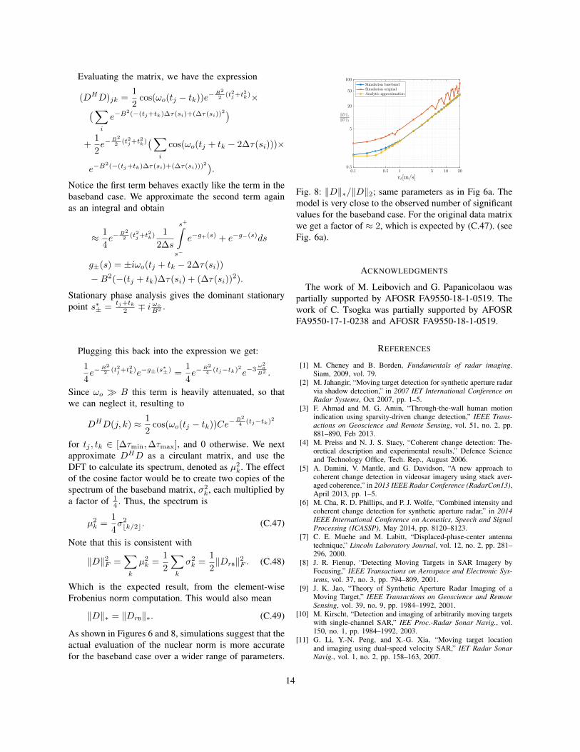
As shown in Figures 6 and 8, simulations suggest that theactual evaluation of the nuclear norm is more accuratefor the baseband case over a wider range of parameters.

Fig. 8: ‖D‖∗/‖D‖2; same parameters as in Fig 6a. Themodel is very close to the observed number of significantvalues for the baseband case. For the original data matrixwe get a factor of ≈ 2, which is expected by (C.47). (seeFig. 6a).

ACKNOWLEDGMENTS

The work of M. Leibovich and G. Papanicolaou waspartially supported by AFOSR FA9550-18-1-0519. Thework of C. Tsogka was partially supported by AFOSRFA9550-17-1-0238 and AFOSR FA9550-18-1-0519.

REFERENCES

[1] M. Cheney and B. Borden, Fundamentals of radar imaging.Siam, 2009, vol. 79.

[2] M. Jahangir, “Moving target detection for synthetic aperture radarvia shadow detection,” in 2007 IET International Conference onRadar Systems, Oct 2007, pp. 1–5.

[3] F. Ahmad and M. G. Amin, “Through-the-wall human motionindication using sparsity-driven change detection,” IEEE Trans-actions on Geoscience and Remote Sensing, vol. 51, no. 2, pp.881–890, Feb 2013.

[4] M. Preiss and N. J. S. Stacy, “Coherent change detection: The-oretical description and experimental results,” Defence Scienceand Technology Office, Tech. Rep., August 2006.

[5] A. Damini, V. Mantle, and G. Davidson, “A new approach tocoherent change detection in videosar imagery using stack aver-aged coherence,” in 2013 IEEE Radar Conference (RadarCon13),April 2013, pp. 1–5.

[6] M. Cha, R. D. Phillips, and P. J. Wolfe, “Combined intensity andcoherent change detection for synthetic aperture radar,” in 2014IEEE International Conference on Acoustics, Speech and SignalProcessing (ICASSP), May 2014, pp. 8120–8123.

[7] C. E. Muehe and M. Labitt, “Displaced-phase-center antennatechnique,” Lincoln Laboratory Journal, vol. 12, no. 2, pp. 281–296, 2000.

[8] J. R. Fienup, “Detecting Moving Targets in SAR Imagery byFocusing,” IEEE Transactions on Aerospace and Electronic Sys-tems, vol. 37, no. 3, pp. 794–809, 2001.

[9] J. K. Jao, “Theory of Synthetic Aperture Radar Imaging of aMoving Target,” IEEE Transactions on Geoscience and RemoteSensing, vol. 39, no. 9, pp. 1984–1992, 2001.

[10] M. Kirscht, “Detection and imaging of arbitrarily moving targetswith single-channel SAR,” IEE Proc.-Radar Sonar Navig., vol.150, no. 1, pp. 1984–1992, 2003.

[11] G. Li, Y.-N. Peng, and X.-G. Xia, “Moving target locationand imaging using dual-speed velocity SAR,” IET Radar SonarNavig., vol. 1, no. 2, pp. 158–163, 2007.

14

[12] J. Ender, “Detectability of slowly moving targets using a multi-channel SAR with an along-track antenna array,” in Proceedingsof SEE/IEE Conference (SAR93), Paris, 1993, pp. 19–22.

[13] ——, “Detection and estimation of moving target signals bymulti-channel sar,” AEU International Journal of ElectronicCommunication, vol. 50, no. 2, pp. 150–156, 1996.

[14] B. Friedlander and B. Porat, “VSAR: a high resolution radarsystem for detection of moving targets,” IEE Proc.-Radar, SonarNavig., vol. 144, no. 4, pp. 205–218, 1997.

[15] G. Wang, X. Xia, and V. Chen, “Dual-Speed SAR Imaging ofMoving Targets,” IEEE Transactions on Aerospace and Elec-tronic Systems, vol. 42, no. 1, pp. 368–379, 2006.

[16] N. Onhon and M. Cetin, “Sar moving target imaging in asparsity-driven framework,” in Proc. SPIE Optics+Photonics,Wavelets and Sparsity XIV, vol. 8138, 2011, p. 813806. [Online].Available: https://doi.org/10.1117/12.893581

[17] M. Cetin, I. Stojanovic, O. Onhon, K. Varshney, S. Samadi,W. C. Karl, and A. S. Willsky, “Sparsity-driven synthetic apertureradar imaging: Reconstruction, autofocusing, moving targets, andcompressed sensing,” IEEE Signal Processing Magazine, vol. 31,no. 4, pp. 27–40, July 2014.

[18] H. Yan, R. Wang, F. Li, Y. Deng, and Y. Liu, “Ground mov-ing target extraction in a multichannel wide-area surveillancesar/gmti system via the relaxed pcp,” IEEE Geoscience andRemote Sensing Letters, vol. 10, no. 3, pp. 617–621, 2012.

[19] H. Yan, F. Li, W. Robert, M. Zheng, C. Gao, and Y. Deng,“Moving targets extraction in multichannel wide-area surveil-lance system by exploiting sparse phase matrix,” IET Radar,Sonar & Navigation, vol. 6, no. 9, pp. 913–920, 2012.

[20] A. Oveis and M. Sebt, “Dictionary-based principal componentanalysis for ground moving target indication by synthetic apertureradar,” IEEE Geoscience and Remote Sensing Letters, vol. 14,no. 9, pp. 1594–1598, 2017.

[21] A. Soganlı and M. Cetin, “Low-rank sparse matrix decomposi-tion for sparsity-driven sar image reconstruction,” in 2015 3rdInternational Workshop on Compressed Sensing Theory and itsApplications to Radar, Sonar and Remote Sensing (CoSeRa).IEEE, 2015, pp. 239–243.

[22] M. Moradikia, S. Samadi, and M. Cetin, “Joint sar imagingand multi-feature decomposition from 2-d under-sampled datavia low-rankness plus sparsity priors,” IEEE Transactions onComputational Imaging, vol. 5, no. 1, pp. 1–16, 2018.

[23] L. Borcea, T. Callaghan, and G. Papanicolaou, “Synthetic aper-ture radar imaging and motion estimation via robust principalcomponent analysis,” SIAM Journal on Imaging Sciences, vol. 6,no. 3, pp. 1445–1476, 2013.

[24] E. J. Candes, X. Li, Y. Ma, and J. Wright, “Robust PrincipalComponent Analysis?” Journal of ACM, vol. 58, no. 1, pp. 1–37, 2009.

[25] Z. Zhou, X. Li, J. Wright, E. Candes, and Y. Ma, “Stable principalcomponent pursuit,” in 2010 IEEE international symposium oninformation theory. IEEE, 2010, pp. 1518–1522.

[26] Z. Lin, M. Chen, and Y. Ma, “The Augmented LagrangeMultiplier Method for Exact Recovery of Corrupted Low-RankMatrices,” ArXiv e-prints, Sep. 2010.

[27] C. Casteel Jr, L. Gorham, M. Minardi, S. Scarborough, K. Naidu,and U. Majumder, “A challenge problem for 2d/3d imaging oftargets from a volumetric data set in an urban environment,” inProceedings of SPIE, vol. 6568, 2007, p. 65680D.

[28] R. M. Gray et al., “Toeplitz and circulant matrices: A review,”Foundations and Trends R© in Communications and InformationTheory, vol. 2, no. 3, pp. 155–239, 2006.

15