IEEE TRANSACTIONS ON ANTENNAS AND PROPAGATION 1

EM-WaveHoltz: A flexible frequency-domainmethod built from time-domain solvers

Zhichao Peng and Daniel Appelo

Abstract—A novel approach to computing time-harmonic so-lutions of Maxwell’s equations by time-domain simulations ispresented. The method, EM-WaveHoltz, results in a positivedefinite system of equations which makes it amenable to iterativesolution with the conjugate gradient method or with GMRES.Theoretical results guaranteeing the convergence of the methodaway from resonances is presented. Numerical examples illus-trating the properties of EM-WaveHoltz are given.

Index Terms—Maxwell equations, iterative method, elec-trochemical analysis, frequency-domain analysis, time-domainanalysis, FDTD methods, discontinuous Galerkin time-domain(DGTD) methods, positive definite

TWO of the main challenges when solving the time-harmonic Maxwell equations at high frequencies are the

indefinite nature of the Maxwell system and the high resolutionrequirement. Without proper preconditioners, iterative solverssuch as GMRES and BICG may converge slowly. Thesechallenges are similar to the ones for solving the Helmholtzequation at high frequencies. Recently, we introduced a scal-able iterative method called WaveHoltz [1] for the Helmholtzequation. In this paper, we introduce the electromagnetic-WaveHoltz (EM-WaveHoltz) method, which can be seen as ageneralization of the WaveHoltz method to the time-harmonic(or frequency-domain) Maxwell equations. The proposed EM-WaveHoltz method converts the frequency-domain problemto a fix point problem in the time-domain. The fixed pointiteration is linear and can be rewritten as a linear system ofequations with a system matrix that is positive definite andthat can therefore be efficiently inverted using standard Krylovmethods such as GMRES.

In the EM-WaveHoltz method, we convert the frequency-domain problem to a time-domain problem by evolving andfiltering Maxwell’s equations with periodic forcing over onetime period. When applied, this filter results in the time-domain solution converging to a fix point where the solutionbecomes equivalent to the solution of the frequency-domainproblem. Salient features of the EM-WaveHoltz method areas follows.

1) The resulting linear system is always positive definite(sometimes symmetric).

2) The EM-WaveHoltz method can be driven by any scal-able time-domain solver, for example the finite differ-ence time-domain (FDTD) method [2] and discontinuousGalerkin time-domain method (DGTD) [3].

Zhichao Peng is with the Department of Mathematics, Michigan StateUniversity, East Lansing, MI 48824.

Daniel Appelo is with the Department of Computational Mathematics,Science & Engineering and the Department of Mathematics, Michigan StateUniversity, East Lansing, MI 48824

Manuscript received March 30, 2021; revised March 30, 2021.

3) A unique feature of the EM-WaveHoltz method is thatit is possible to obtain frequency-domain solutions formultiple frequencies at once but at the cost of a singlesolve.

We note that properties of our method are to some extentshared with the properties of the controllability method. Inparticular the controllability method finds the solution tothe frequency-domain problem by using time-domain solverslike our approach. However, while our formulation relies ona fixed point iteration, the controllability method seeks tominimize the deviation from time-periodicity of the initial andfinal data of the time-domain simulation. The controllabilitymethod was first proposed for a time-harmonic wave scatteringproblem [4], and we refer readers to [5] for recent devlopment.The controllability method is also generalized to the time-harmonic Maxwell equation in the second order formulation[6] and the first formulation [7], [8]. One main differencebetween our method and the controllability method is thatthe controllability method needs backward solves, while ourmethod does not.

There are of course many other methods that have been de-signed for efficiently solving the frequency-domain Maxwell’sequations. For scattering and radiation problems in homoge-nous media integral equation formulations are known to behighly efficient and yield fast algorithms [9], [10]. Domain de-composition methods (DDM) [11] have also achieved successfor the time-harmonic electromagnetic problems [12], [13],[14], [15], [16]. The DDM method and the integral equationmethod have been combined in [17]. Recently, [18] extends the“shifted-Laplacian preconditioner” for the Helmholtz equationto the high frequency time-harmonic Maxwell equations anddesigns an optimal DDM method. Multigrid methods havealso been considered for the time-harmonic Maxwell equations[19], [20]. A multigrid method for the high frequency time-harmonic Maxwell equations is designed in [21]. Sweepingpreconditioners for time-harmonic Maxwell equations, whichutilize the intrinsic structure of the Green’s function, havebeen developed for the Yee scheme [22] and the finite elementmethod [23].

The rest of this paper is organized as follows. In Section I,we present the EM-WaveHoltz formulation for the continuousequations and discuss the properties of the resulting linearsystem, the choice of the linear solver, and present how toobtain solutions for multiple frequencies in one solve. In Sec-tion II, to show the flexibility with respect to the choice of thetime-domain solvers, we couple the EM-WaveHoltz method,first with the Yee scheme and then with the discontinuousGalerkin (DG) method. In Section III, the performance of the

arX

iv:2

103.

1478

9v1

[m

ath.

NA

] 2

7 M

ar 2

021

IEEE TRANSACTIONS ON ANTENNAS AND PROPAGATION 2

EM-WaveHoltz method is demonstrated through a series ofnumerical examples.

I. ELECTROMAGNETIC WAVEHOLTZ ITERATION FOR THEMAXWELL’S EQUATION

We consider the frequency-domain Maxwell’s equation:

iωεE = ∇×H− J, (1a)iωµH = −∇×E, (1b)

closed by boundary conditions corresponding to either aperfect electric conductor or to an unbounded domain. HereE and H are the complex valued electric and magnetic fieldsand J is the real valued current source. Taking the real andimaginary parts we find

−ω=εE = <∇×H − J, (2a)ω<εE = =∇×H, (2b)

−ω=µH = −<∇×E, (2c)ω<µH = −=∇×E. (2d)

We want to relate the fields E and H to real valued andT = 2π/ω-periodic solutions

E = E0 cos(ωt) + E1 sin(ωt), (3a)

H = H0 cos(ωt) + H1 sin(ωt), (3b)

to the time-domain equations

ε∂tE = ∇× H− sin(ωt)J, (4a)

µ∂tH = −∇× E. (4b)

For such periodic solutions we can match the sin(ωt) andcos(ωt) terms to find the relations

εω(−E0) = ∇× H1 − J,

εω(E1) = ∇× H0,

µω(−H0) = −∇× E1,

µω(H1) = −∇× E0.

It now follows that the initial data of E and H determines theimaginary part of the frequency-domain solution

=E = E0, =H = H0,

as well as the real part

<E = E1 =1

ε∇× H0, <H = H1 = − 1

µ∇× E0.

(5)

Our EM-WaveHoltz method finds the periodic solutions (3)by iteratively determining the initial data,

E|t=0 = νE = E0, H|t=0 = νH = H0,

to (4). Define the filtering operator, Π, acting on the initialconditions ν = (νE ,νH)T :

Πν = Π

(νEνH

)=

2

T

∫ T

0

(cos(ωt)− 1

4

)(E

H

)dt, (6)

with T = 2π/ω.

By construction, one can verify that Π(=E,=H)T =(=E,=H)T . As the real part can be computed directlyvia (5), the solution to the frequency-domain equation is a fix-point of the operator Π. Based on these facts, we define theEM-WaveHoltz iteration:

Πνn+1 = Πνn, with ν0 = (ν0E ,ν

0H)T = 0. (7)

The EM-WaveHoltz iteration converges to the imaginary partsof the solution to the frequency-domain equation

limn→∞

νn = limn→∞

(νnE ,νnH)T = (=E,=H)T , (8)

and the real parts can be recovered via (5).

Remark 1. Alternatively we could formulate the time-domainproblem with a cosine forcing

ε∂tE = ∇× H− cos(ωt)J, (9a)

µ∂tH = −∇× E. (9b)

Again, the real valued T = 2π/ω-periodic solutions to (9) areon the form (3) but (see Appendix A) the solution to (9) E andH have a slightly different relation to the frequency-domainsolution

<E = E0, <H = H0, =E = −E1, =H = −H1.

With the same filter and iteration process defined as the sin-forcing case, we have

limn→∞

νn = limn→∞

(νnE ,νnH)T = (<E,<H)T . (10)

In our numerical tests, we find that the number of iterationsneeded by the EM-WaveHoltz method are essentially identicalfor the two alternatives. In this paper, we focus on the EM-Waveholtz with the sin-forcing.

A. EM-WaveHoltz for the energy conserving case

For PEC boundary conditions and other boundary condi-tions that lead to a conservation of the electromagnetic energyin a bounded domain, the EM-WaveHoltz iteration can besimplified further. For such problems =H is identically zeroand the EM-WaveHoltz iteration is reduced to

νn+1E = ΠνnE , νnH = 0, ν0

E = 0, (11)

where now

ΠνE =2

T

∫ T

0

(cos(ωt)− 1

4

)Edt. (12)

As long as ω is not a resonance this simplified EM-WaveHoltziteration converges

νnE = =E, as n→∞. (13)

IEEE TRANSACTIONS ON ANTENNAS AND PROPAGATION 3

B. Krylov acceleration

For bounded problems where ω is close to a resonanceor for unbounded problems with trapping geometries, theconvergence of the WaveHoltz fix point iteration can beslow [1]. Fortunately as the iteration is linear, it is easy torewrite it as a positive definite linear operator that can beefficiently inverted by a Krylov subspace method. To see thiswe introduce the operator:

Sν = Πν −Π0. (14)

Then, based on the definition of S, we have

Πν = Sν + Π0. (15)

Hence, finding the fix point of Π: Πν = ν is equivalent tosolving the equation (I − S)ν = Π0.

A Krylov method such as the conjugate gradient method,GMRES or TFQMR can be applied to solve (I − S)ν = Π0in a matrix-free manner. In practice, to obtain the right handside Π0, we just need to solve the time-domain problem (4)with zero initial conditions ν = 0 from t = 0 to t = T anduse a numerical quadrature to approximate the filter Π0 as wemarch in time. To calculate the matrix multiplication (I−S)ν,we can utilize the fact that

(I − S)ν = ν − (Πν −Π0) = ν −Πν + Π0.

That is, for a given ν and Π0 precomputed, we just need tocompute Πν to obtain the action of (I − S) onto ν. Recallthat Πν is obtained by computing the filter by a numericalquadrature incrementally as the solution to (4) is evolved forone T = 2π/ω period with ν as the initial conditions. Thusthe cost to compute one Krylov vector is that of a wave solvewith one additional variable needed to sum up the projectionthroughout the evolution.

When using GMRES there is always a concern about thesize of the Krylov subspace as the number of iterations grow.Here our method has a significant upside to solving thefrequency-domain problem. Note that although we are lookingfor a T = 2π

ω -periodic solution, there is nothing in the methodthat prevents us from changing the filtering to extend over alonger time, say, T = N 2π

ω , with N a positive integer. Aswe show in the numerical examples below, for moderate Nthis reduces the number of iterations by a factor of N so thatthe overall computational cost is the same. However, using alonger iteration with N > 1 reduces the size of the GMRESKrylov subspace by a factor of N compared to a frequency-domain iteration.

In Appendix B, we show that I−S is always a positive defi-nite operator and for energy conserving boundary conditions itis also self-adjoint. These results carry over to the discretizedequations in the sense that the matrix that needs to be invertedis always positive definite and, if a symmetric and energyconserving method (like the Yee scheme) is used, the matrixis also symmetric for energy conserving boundary conditionslike PEC. For the SPD case our method becomes particularlyefficient and memory lean as the conjugate gradient methodcan be used.

C. Multiple frequencies in one solve

Similar to the WaveHoltz method for the Helmholtz equa-tion [1], the EM-WaveHoltz method can be applied to obtainthe solutions for multiple frequencies in one solve.

Precisely, let ωk = nkω0, k = 1, . . . , N for some ω0 > 0and n1 < n2 < · · · < nN being positive integers. Then ina traditional frequency-domain solver each frequency requiresthe solution of N different systems

iωkεEk = ∇×Hk − Jk, (16a)iωkµHk = −∇×Ek. (16b)

Now, assuming that each frequency solve has the same typeof boundary condition and material properties (the forcing Jkcan be different for each k), we can solve for all frequenciesat once. We take the energy conserving case as an example,then the single time-domain problem we must solve is

ε∂tE = ∇× H−N∑k=1

sin(ωkt)Jk, (17a)

µ∂tH = ∇× E. (17b)

The converged solution to (17) can be decomposed as

E =

N∑k=1

Ek,0 cos(ωkt), (18)

where Ek,0 = =Ek gives the solution to the originalfrequency-domain problem (16) corresponding to ωk. To ob-tain the “all k” solution through EM-WaveHoltz is easy, thefiltering operator simply needs to be modified as

ΠνE =2

T

∫ T

0

(N∑k=1

cos(ωkt)−1

4

)Edt. (19)

Here, the final time T is chosen such that T/( 2πωk

) is an integerfor all k.

Once the EM-WaveHoltz iteration has converged to (18) weseparate the different solutions by evolving (16) for one moreTk-period while applying the filters

=(Ek) =2

Tk

∫ Tk

0

(cos(ωkt)−

1

4

)Edt, (20)

<(Ek) =2

Tk

∫ Tk

0

sin(ωkt) Edt. (21)

II. DISCRETIZATION OF THE EM-WAVEHOLTZ METHOD

We have presented how the EM-WaveHoltz iteration con-verts a frequency-domain problem to a time-domain problem.In this section, we will use the Yee scheme [24], [25] andthe discontinuous Galerkin (DG) method [3], [26], [27] asexamples of integrating the EM-WaveHoltz iteration in ex-isting time-domain solvers. We also want to point out thatit is possible to couple the EM-WaveHoltz method to othertype time-domain solvers such as spectral element method andcontinuous finite element method. Further, although we don’tconsider it here, our approach directly generalizes to lineardispersive frequency-domain models such as the generalizeddispersive materials modeled through an auxiliary differentialequation approach in [28].

IEEE TRANSACTIONS ON ANTENNAS AND PROPAGATION 4

A. Yee-EM-WaveHoltz

The Yee scheme [24], [25] or the finite-difference-time-domain (FDTD) method, is one of the most popular andsuccessful methods in computational electromagnetics and canbe easily turned into a fast FDFD method, the Yee-EM-WaveHoltz method, as follows.

Assume a uniform time step size ∆t = T/M and denoteany given function at a point (i∆x, j∆y, k∆z, n∆t) in (3+1)dimensions by

Fni,j,k = F (i∆x, j∆y, k∆z, n∆t). (22)

Also denote any point in time n∆t = tn. Then the Yee schemeto solve the time-domain problem in the EM-WaveHoltzformulation is

(Hx)n+ 1

2

i,j+ 12 ,k+ 1

2

− (Hx)n− 1

2

i,j+ 12 ,k+ 1

2

∆t

=1

µi,j+ 12 ,k+ 1

2

( (Ey)ni,j+ 1

2 ,k+1− (Ey)n

i,j+ 12 ,k

∆z

−(Ez)

ni,j+1,k+ 1

2

− (Ez)ni,j,k+ 1

2

∆y

), (23a)

(Hy)n+ 1

2

i+ 12 ,j,k+ 1

2

− (Hy)n− 1

2

i+ 12 ,j,k+ 1

2

∆t

=1

µi+ 12 ,j,k+ 1

2

( (Ez)ni+1,j,k+ 1

2

− (Ez)ni,j,k+ 1

2

∆x

−(Ex)n

i+ 12 ,j,k+1

− (Ex)ni+ 1

2 ,j,k

∆z

). (23b)

(Hz)n+ 1

2

i+ 12 ,j+

12 ,k− (Hz)

n− 12

i+ 12 ,j+

12 ,k

∆t

=1

µi+ 12 ,j+

12 ,k

( (Ex)ni+ 1

2 ,j+1,k− (Ex)n

i+ 12 ,j,k

∆y

−(Ey)n

i+1,j+ 12 ,k− (Ey)n

i,j+ 12 ,k

∆x

), (23c)

and

εi+ 12 ,j,k

(Ex)n+1i+ 1

2 ,j,k− (Ex)n

i+ 12 ,j,k

∆t= −sin(ωtn+ 1

2 )(Jx)i+ 12 ,j,k

+( (Hz)

n+ 12

i+ 12 ,j+

12 ,k− (Hz)

n+ 12

i+ 12 ,j−

12 ,k

∆y

−(Hy)

n+ 12

i+ 12 ,j,k+ 1

2

− (Hy)n+ 1

2

i+ 12 ,j,k−

12

∆z

), (24a)

εi,j+ 12 ,k

(Ey)n+1i,j+ 1

2 ,)− (Ey)n

i,j+ 12 ,k

∆t= −sin(ωtn+ 1

2 )(Jy)i,j+ 12 ,k

+( (Hx)

n+ 12

i,j+ 12 ,k+ 1

2

− (Hx)ni,j+ 1

2 ,k−12

∆z

−(Hz)

n+ 12

i+ 12 ,j,k+ 1

2

− (Hz)n+ 1

2

i− 12 ,j,k+ 1

2

∆x

), (24b)

εi,j,k+ 12

(Ez)n+1i,j,k+ 1

2

− (Ez)ni,j,k+ 1

2

∆t= −sin(ωtn+ 1

2 )(Jz)i,j,k+ 12

+( (Hy)

n+ 12

i+ 12 ,j,k+ 1

2

− (Hy)n+ 1

2

i− 12 ,j,k+ 1

2

∆x

−(Hx)

n+ 12

i,j+ 12 ,k+ 1

2

− (Hx)n+ 1

2

i,j− 12 ,k+ 1

2

∆y

). (24c)

For the initial step H−12

x is initialized as

(Hx)− 1

2

i,j+ 12 ,k+ 1

2

= (Hx)0i,j+ 1

2 ,k+ 12

− ∆t

2µi,j+ 12 ,k+ 1

2

( (Ey)0i,j+ 1

2 ,k+1− (Ey)0

i,j+ 12 ,k

∆z

−(Ez)

0i,j+1,k+ 1

2

− (Ez)0i,j,k+ 1

2

∆y

), (25)

and H−12

y and H−12

z are initialized similarly.To approximate the filter operator Π in (26) we use the

composite trapezoidal rule

Πh

(νEνH

)=

2∆t

T

M∑n=0

ηn

(cos(ωtn)− 1

4

)(En

Hn+12 +Hn− 1

2

2

),

(26)

where

ηn =

12 , n = 0 or M,

1, otherwise.(27)

The solution obtained by the above iteration introducesan additional error from the time marching and as a resultconverges to a frequency-domain solution with a sightly per-turbed frequency ω, where |ω − ω| = O(∆t2). Of coursesince ∆t ∼ min∆x,∆y,∆z the EM-WaveHoltz solution isconverging at the same rate as the spatial discreization butnevertheless it does have an additional error. This error iseasily eliminated by a small modification which we discussnext.

B. Eliminating the temporal error in EM-WaveHoltz

For brevity we consider the energy conserving two di-mensional TM model. Then Ex = Ey = Hz = 0 andwe can neglect the k component. The Yee scheme for thecorresponding time-domain equation is defined as:

εi,j(Ez)

n+1i,j − (Ez)

ni,j

∆t=( (Hy)

n+ 12

i+ 12 ,j− (Hy)

n+ 12

i− 12 ,j

∆x

−(Hx)

n+ 12

i,j+ 12

− (Hx)n+ 1

2

i,j− 12

∆y

)− Sn+ 1

2 (Jz)i,j (28)

IEEE TRANSACTIONS ON ANTENNAS AND PROPAGATION 5

and

(Hx)n+ 1

2

i,j+ 12

− (Hx)n− 1

2

i,j+ 12

∆t= − 1

µi,j+ 12

(Ez)ni,j+1 − (Ez)

ni,j

∆y,

(29a)

(Hy)n+ 1

2

i+ 12 ,j− (Hy)

n− 12

i+ 12 ,j

∆t=

1

µi+ 12 ,j

(Ez)ni+1,j − (Ez)

ni,j

∆x,

(29b)

with initial conditions E0z = ν and H0

x = H0y = 0. H−

12

x and

H− 1

2y are initialized similar to (25). Here, the slight modifica-

tion is that we use the second order accurate approximation

S12 =

ω∆t

2, Sn+ 1

2 = Sn−12 + ∆tω cos(ωtn), (30)

to sin(ωtn+ 12 ). Using Sn+ 1

2 instead of sin(ωtn+ 12 ) gives us a

chance to eliminate the error due to the time discretization.Eliminating Hx and Hy in (28) and (29), we have

(Ez)n+1i,j − 2(Ez)

ni,j + (Ez)

n−1i,j

∆t2+ Lh(Ez)

ni,j

=− (1

εi,jJz)i,j

Sn+ 12 − Sn− 1

2

∆t

=− (1

εi,jJz)i,j cos(ωtn), (31)

where

−LhFi,j =1

εi,j∆x

(Fi+1,j − Fi,jµi+ 1

2 ,j∆x

− Fi,j − Fi−1,j

µi− 12 ,j

∆x

)+

1

εi,j∆y

(Fi,j+1 − Fi,jµi,j+ 1

2∆y

− Fi,j − Fi,j−1

µi,j− 12∆y

). (32)

(31) is an approximation to the second order form of the time-domain equation in EM-WaveHoltz. We now have the fol-lowing theorem guaranteeing the convergence of the discreteiteration (for the energy conserving case)

Theorem 1. Let ν∞ be the solution to

ω2ν∞ − Lhν∞ = ω

(1

εJ

), ω =

sin(ω∆t/2)

∆t/2. (33)

Further, let −λ2jNj=1 and ψjNj=1 be the eigenvalues and

corresponding eigenfunctions of Lh, and 0 < λ1 < λ2 <· · · < λN . Assume that ω is not a resonance and denote therelative distance to the closest resonance δh = minj |λj −ω|/ω > 0.

Then, for the energy conserving method, (28) - (29), with thefilter (26), the Yee-EM-WaveHoltz iteration ν(k+1) = Πhν

(k)

with ν(0) = 0 converges to ν∞ as long as

∆t ≤ 2

λN + 2ω/π, ω∆t ≤ min(δh, 1). (34)

Moreover, the convergence rate is at least ρh = max(1 −0.3δ2

h, 0.6).

The proof of this Theorem is presented in Appendix C.We note that the first constraint on the timestep is essentially

the standard CFL condition for an explicit method while the

second condition could be very strict. In actual computationswe never observe that violation of the second condition leadsto problems and conjecture that it is likely a mathematicalartifact rather than a practical limitation.

Now, if we replace cos(ωtn) with cos(ωtn) in (30) with

ω =2

∆tsin−1

(ω∆t

2

), (35)

and modify the trapezoidal weights in the filter as

Πhν =2∆t

T

M∑n=0

(cos(ωtn)− 1

4

)cos(ωtn)

cos(ωtn)Enz . (36)

Then Theorem 1 holds but the convergence is to ν∞ being thesolution to the standard discretized frequency-domain problem

ω2ν∞ − Lhν∞ = ω

(1

εJ

). (37)

The derivation of this strategy is discussed in Appendix Dalong with the proof of Theorem 1.

C. DG-EM-WaveHoltz

The discontinuous Galerkin (DG) method, due to its highorder accuracy, flexibility to use nonconforming meshes andits suitability for parallel implementation, has become in-creasingly popular for the simulation of time-domain wavepropagation. As for the Yee scheme, DGTD can easily beturned into a frequency-domain solver using our approach.Here we use the time-domain DG method of [3], [26].

Consider Maxwell’s equation in d-dimensions. Let Ωj bean element, and P s(Ωj) be the space of polynomials atmost degree s. Define V sh (Ωj) =

(P s(Ωj)

)dto be the

corresponding vector polynomial space. The DG method seeksthe solution Eh ∈ V sh (Ωj), Hh ∈ V sh (Ωj) such that for anyφ ∈ V sh (Ωj), ψ ∈ V sh (Ωj)∫

Ωj

∂tEh · φdV =

∫Ωj

Hh · ∇ × (1

εφ)dV

+

∫∂Ωj

(H× n) · (1

εφ)ds−

∫Ωj

sin(ωt)J · φdV, (38a)

∫Ωj

∂tHh ·ψdV = −∫

Ωj

Eh · ∇ × (1

µψ)dV

−∫∂Ωj

(E× n) · ( 1

µψ)ds. (38b)

Here, n is the outward pointing normal of a face and H andE are numerical fluxes. A stable and accurate choice for thenumerical fluxes is

H = H+ α[E], E = E+ β[H]. (39)

Here v± denotes the two values on each side of a face, v =12 (v++v−) is the average and [v] = n+×v++n−×v− is thejump. The semi-discretization (38) can be evolved in a methodof lines fashion, using for example a Runge-Kutta method asthe time stepper. Depending on the time discretization it maybe possible to eliminate the time error as discussed above butwe don’t pursue this here. Further, in the examples below wealways use the trapezoidal rule to discretize the filter.

IEEE TRANSACTIONS ON ANTENNAS AND PROPAGATION 6

III. NUMERICAL RESULTS

In this section we demonstrate the performance of theEM-WaveHoltz methods on several examples in two andthree dimensions. The sin-forcing formulation is used in twodimensions and the cos-forcing formulation is used in threedimensions, unless otherwise specified.

A. Accuracy test in two dimensions with Yee-EM-WaveHoltz

As a first test we solve the 2D TM model. We non-dimensionalize the equations so that ε = µ = 1 and manu-facture a forcing such that the exact solution is Ez(x, y) =16x2(x − 1)2y2(y − 1)2. This solution is compatible withperfect electric conductor (PEC) boundary conditions on thedomain [0, 1]2. We apply the Yee scheme and the EM-WaveHoltz iteration with GMRES acceleration.

To test the convergence for a) one frequency in one solve,and b) multiple frequencies in one solve, we perform a gridrefinement study at fixed frequencies ω1 = 5.5, 3ω1 and 7ω1.In Figure 1, we display how the error is decreased as the gridsize is reduced. As expected, for both of one frequency inone solve and multiple frequencies in one solve, we observesecond order convergence. However, there is a difference inthe amplitude of the error between the solutions obtained usingthe two approaches. For the same frequency, one frequency inone solve is more accurate than multiple frequencies in onesolve.

Fig. 1. Grid convergence of a manufactured solution. Here “o” stands forone frequency in one solve, and “m” stands for multiple frequencies in onesolve. The errors displayed are for Ez for a 2D TM model.

B. Eliminating the temporal error in Yee-EM-WaveHoltz

Again, let ε = µ = 1 and consider the 2D TM modelon the domain [0, 1]2. We choose the forcing and the non-zero Dirichlet boundary conditions so that the exact solutionis Ez(x, y) = x + y. As this is a polynomial with totaldegree one, the spatial part of the Yee scheme is exact andwe should be able to fully eliminate all errors by using themodified quadrature designed to eliminate the temporal error.To recap, in the modification we apply Sn+ 1

2 in (30) with the

frequency modification (35) to approximate sin(ωtn+ 12 ) and

use the modified numerical quadrature (36).To confirm that the temporal error is eliminated we compute

solutions for the frequencies ω = 10.5, 20.5, 30.5, 40.5, 50.5on a grid with 20 gridpoints in each direction using theGMRES accelerated Yee-EM-WaveHoltz iteration.

TABLE ICONFIRMATION OF THE ELIMINATION OF THE TEMPORAL ERRORS FOR

THE YEE-EM-WAVEHOLTZ METHOD WHEN THE MODIFIED QUADRATUREIS USED. THE ERRORS ARE FOR Ez AND FOR DIFFERENT FREQUENCIES.

ω 10.5 20.5 30.5 40.5 50.5Error 1.03E-13 4.65E-13 4.43E-13 6.07E-13 3.83E-13

The results, presented in Table I, show that the modifiedquadrature does eliminate the temporal errors.

C. Number of iterations for different frequencies and bound-ary conditions in two dimensions

In this experiment we solve the 2D TM model with thesource

Jz = −ω exp(−σ((x− 0.01)2 + (y − 0.015)2)

), (40)

where σ = max(36, ω2), ε = µ = 1, and the computationaldomain is [−1, 1]2. Here we sweep over the frequenciesω = k + 1

2 , 1 ≤ k ≤ 100. We use the GMRES acceleratedYee-EM-WaveHoltz iteration and to keep the solution reason-ably well resolved we use 8dωe grids in each directions.

We solve this problem with 6 different boundary conditions:(1) 4 open boundaries, (2) 1 PEC boundary and 3 open bound-aries, (3) 2 parallel PEC boundaries and 2 open boundaries, (4)2 PEC boundaries next to each other forming a PEC cornerand 2 open boundaries, (5) 3 PEC boundaries and 1 openboundary, (6) 4 PEC boundaries. The rationale here is that inproblems (1), (2) and (4) there will not be any opposing PECwalls where waves can be “trapped” while in the other threeproblems there are.

Fig. 2. Number of iterations as a function of frequency for the six different2D TM problems.

We also note that in the open directions we employ theoptimally accurate double absorbing boundary layer (DAB) by

IEEE TRANSACTIONS ON ANTENNAS AND PROPAGATION 7

Hagstrom et al. [29]. The order of approximation in the DABlayers we use is 10 which virtually makes the non-reflectingboundary conditions exact.

In the EM-WaveHoltz iteration, we use 10 periods so thatT = 10 2π

ω . This reduces the memory consumption in GMRESby a factor 10 and reduces the number of iterations by nearlya factor of 10 (the cost per iteration of course goes up by 10as well). In Fig. 2, the number of iteration required to reducethe relative residual below 10−7 are presented. We observethat for the problems without trapped waves, the number ofiterations scales approximately as ω0.9. For the problems withtrapped waves, the iteration converges slower and the numberof iterations scales as approximately ω1.8.

D. Number of iterations for different frequencies and bound-ary conditions in three dimensions

In this example we solve the 3D Maxwell’s equation witha source

Jx = −ω exp(−σ(x2 + y2 + z2)

), Jy = Jz = 0. (41)

Here σ = max(36, ω2), ε = µ = 1 and the computationaldomain is [−1, 1]3.

To measure how the number of iterations grow with thefrequency, three different problems are considered: (1) an opendomain, (2) two parallel PEC plates, (3) five PEC boundariesand one free side on the most left side. Again, we still applythe highly accurate double absorbing boundary layer (DAB)for non-reflecting boundary conditions. The order of the DABlayers is set as 5 guaranteeing that the error of the non-reflecting boundary conditions is well below the discretizationerror.

We sweep over frequencies and use the GMRES acceleratedYee-EM-WaveHoltz method with the cos-forcing. To have awell resolved solution we use 4dωe elements in each direction.In the EM-WaveHoltz iteration, we set T as 5 periods.

In Figure 3, iteration numbers to reduce the relative residualbelow 10−6 are presented. The total number of iterations isestimated to scale as ω0.9 for the open problem, ω1.9 for theparallel PEC plate problem and ω2.5 for the problem with onefree side.

We also use the the sin-forcing to simulate the open domainproblem with the same mesh and the error tolerance. Weobserve that the number of iteration is exactly the same as thecos-forcing, though the relative residual is slightly differentfor high frequencies.

E. Smaller Krylov subspaces by longer filter time

As we mentioned before, we can filter over multiple periodsT = N 2π

ω , which allows the further propagation of the wave.We consider T = N 2π

ω with N = 1, 3, 5 for 2D and 3Dopen domain problem. The setup of this test is the same asSection III-C for 2D and Section III-D for 3D. We scan overdifferent frequencies and apply the GMRES accelerated Yee-EM-WaveHoltz. The total number of iteration allowed is setas 200 in 2D and 100 in 3D. As can be seen in Figure 4for high frequencies both the 2D and the 3D solver, when

Fig. 3. Number of iterations as a function of frequency for different 3Dproblems.

using T = 2πω , fails to converge to the desired tolerance before

reaching the maximum number of iterations.In Figure 4, we present unscaled number of iterations

against the frequency and observe that the number of iterationsdecays as the propagation time T in the time-domain grows.To further quantify the relation between the computational costand T = N 2π

ω , we scale the number of iterations by N andpresent the result in Figure 5. We observe that for N = 3and 5 the scaled curves collapse, implying that the the totalcomputational time is approximately the same. Thus, withoutincreasing the computational cost, filtering over longer timecan decrease the number of iterations, which in turn reducesthe size of the Krylov subspace used by GMRES.

Fig. 4. Unscaled number of iterations as a function of frequency for differentfiltering time. Top: 2D open problem. Bottom: 3D open problem.

Fig. 5. Scaled number of iterations = N× number of iterations, if T = N 2πω

.Scaled number of iterations as a function of frequency for different filteringtime. Top: 2D open problem. Bottom: 3D open problem.

IEEE TRANSACTIONS ON ANTENNAS AND PROPAGATION 8

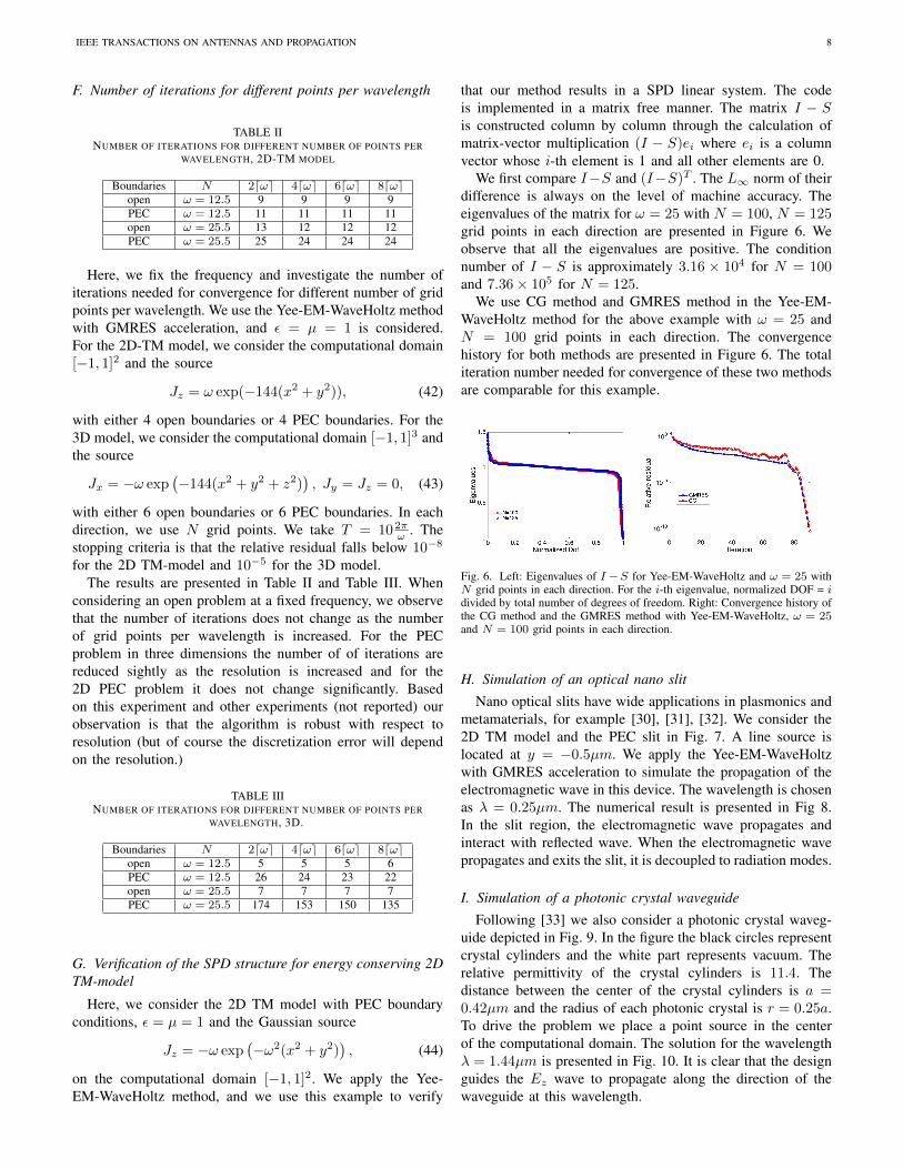
F. Number of iterations for different points per wavelength

TABLE IINUMBER OF ITERATIONS FOR DIFFERENT NUMBER OF POINTS PER

WAVELENGTH, 2D-TM MODEL

Boundaries N 2dωe 4dωe 6dωe 8dωeopen ω = 12.5 9 9 9 9PEC ω = 12.5 11 11 11 11open ω = 25.5 13 12 12 12PEC ω = 25.5 25 24 24 24

Here, we fix the frequency and investigate the number ofiterations needed for convergence for different number of gridpoints per wavelength. We use the Yee-EM-WaveHoltz methodwith GMRES acceleration, and ε = µ = 1 is considered.For the 2D-TM model, we consider the computational domain[−1, 1]2 and the source

Jz = ω exp(−144(x2 + y2)), (42)

with either 4 open boundaries or 4 PEC boundaries. For the3D model, we consider the computational domain [−1, 1]3 andthe source

Jx = −ω exp(−144(x2 + y2 + z2)

), Jy = Jz = 0, (43)

with either 6 open boundaries or 6 PEC boundaries. In eachdirection, we use N grid points. We take T = 10 2π

ω . Thestopping criteria is that the relative residual falls below 10−8

for the 2D TM-model and 10−5 for the 3D model.The results are presented in Table II and Table III. When

considering an open problem at a fixed frequency, we observethat the number of iterations does not change as the numberof grid points per wavelength is increased. For the PECproblem in three dimensions the number of of iterations arereduced sightly as the resolution is increased and for the2D PEC problem it does not change significantly. Basedon this experiment and other experiments (not reported) ourobservation is that the algorithm is robust with respect toresolution (but of course the discretization error will dependon the resolution.)

TABLE IIINUMBER OF ITERATIONS FOR DIFFERENT NUMBER OF POINTS PER

WAVELENGTH, 3D.

Boundaries N 2dωe 4dωe 6dωe 8dωeopen ω = 12.5 5 5 5 6PEC ω = 12.5 26 24 23 22open ω = 25.5 7 7 7 7PEC ω = 25.5 174 153 150 135

G. Verification of the SPD structure for energy conserving 2DTM-model

Here, we consider the 2D TM model with PEC boundaryconditions, ε = µ = 1 and the Gaussian source

Jz = −ω exp(−ω2(x2 + y2)

), (44)

on the computational domain [−1, 1]2. We apply the Yee-EM-WaveHoltz method, and we use this example to verify

that our method results in a SPD linear system. The codeis implemented in a matrix free manner. The matrix I − Sis constructed column by column through the calculation ofmatrix-vector multiplication (I − S)ei where ei is a columnvector whose i-th element is 1 and all other elements are 0.

We first compare I−S and (I−S)T . The L∞ norm of theirdifference is always on the level of machine accuracy. Theeigenvalues of the matrix for ω = 25 with N = 100, N = 125grid points in each direction are presented in Figure 6. Weobserve that all the eigenvalues are positive. The conditionnumber of I − S is approximately 3.16 × 104 for N = 100and 7.36× 105 for N = 125.

We use CG method and GMRES method in the Yee-EM-WaveHoltz method for the above example with ω = 25 andN = 100 grid points in each direction. The convergencehistory for both methods are presented in Figure 6. The totaliteration number needed for convergence of these two methodsare comparable for this example.

Fig. 6. Left: Eigenvalues of I −S for Yee-EM-WaveHoltz and ω = 25 withN grid points in each direction. For the i-th eigenvalue, normalized DOF = idivided by total number of degrees of freedom. Right: Convergence history ofthe CG method and the GMRES method with Yee-EM-WaveHoltz, ω = 25and N = 100 grid points in each direction.

H. Simulation of an optical nano slit

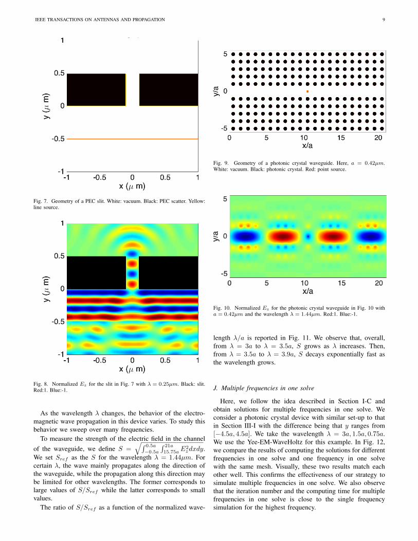
Nano optical slits have wide applications in plasmonics andmetamaterials, for example [30], [31], [32]. We consider the2D TM model and the PEC slit in Fig. 7. A line source islocated at y = −0.5µm. We apply the Yee-EM-WaveHoltzwith GMRES acceleration to simulate the propagation of theelectromagnetic wave in this device. The wavelength is chosenas λ = 0.25µm. The numerical result is presented in Fig 8.In the slit region, the electromagnetic wave propagates andinteract with reflected wave. When the electromagnetic wavepropagates and exits the slit, it is decoupled to radiation modes.

I. Simulation of a photonic crystal waveguide

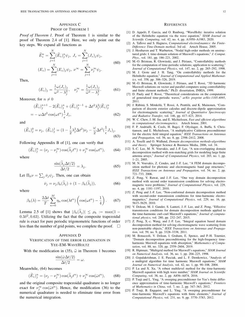
Following [33] we also consider a photonic crystal waveg-uide depicted in Fig. 9. In the figure the black circles representcrystal cylinders and the white part represents vacuum. Therelative permittivity of the crystal cylinders is 11.4. Thedistance between the center of the crystal cylinders is a =0.42µm and the radius of each photonic crystal is r = 0.25a.To drive the problem we place a point source in the centerof the computational domain. The solution for the wavelengthλ = 1.44µm is presented in Fig. 10. It is clear that the designguides the Ez wave to propagate along the direction of thewaveguide at this wavelength.

IEEE TRANSACTIONS ON ANTENNAS AND PROPAGATION 9

Fig. 7. Geometry of a PEC slit. White: vacuum. Black: PEC scatter. Yellow:line source.

Fig. 8. Normalized Ez for the slit in Fig. 7 with λ = 0.25µm. Black: slit.Red:1. Blue:-1.

As the wavelength λ changes, the behavior of the electro-magnetic wave propagation in this device varies. To study thisbehavior we sweep over many frequencies.

To measure the strength of the electric field in the channelof the waveguide, we define S =

√∫ 0.5a

−0.5a

∫ 21a

15.75aE2zdxdy.

We set Sref as the S for the wavelength λ = 1.44µm. Forcertain λ, the wave mainly propagates along the direction ofthe waveguide, while the propagation along this direction maybe limited for other wavelengths. The former corresponds tolarge values of S/Sref while the latter corresponds to smallvalues.

The ratio of S/Sref as a function of the normalized wave-

Fig. 9. Geometry of a photonic crystal waveguide. Here, a = 0.42µm.White: vacuum. Black: photonic crystal. Red: point source.

Fig. 10. Normalized Ez for the photonic crystal waveguide in Fig. 10 witha = 0.42µm and the wavelength λ = 1.44µm. Red:1. Blue:-1.

length λ/a is reported in Fig. 11. We observe that, overall,from λ = 3a to λ = 3.5a, S grows as λ increases. Then,from λ = 3.5a to λ = 3.9a, S decays exponentially fast asthe wavelength grows.

J. Multiple frequencies in one solve

Here, we follow the idea described in Section I-C andobtain solutions for multiple frequencies in one solve. Weconsider a photonic crystal device with similar set-up to thatin Section III-I with the difference being that y ranges from[−4.5a, 4.5a]. We take the wavelength λ = 3a, 1.5a, 0.75a.We use the Yee-EM-WaveHoltz for this example. In Fig. 12,we compare the results of computing the solutions for differentfrequencies in one solve and one frequency in one solvewith the same mesh. Visually, these two results match eachother well. This confirms the effectiveness of our strategy tosimulate multiple frequencies in one solve. We also observethat the iteration number and the computing time for multiplefrequencies in one solve is close to the single frequencysimulation for the highest frequency.

IEEE TRANSACTIONS ON ANTENNAS AND PROPAGATION 10

Fig. 11. Displayed is S as a function of the wavelength in the photonic crystalwaveguide. Here, a = 0.42µm, and Sref is obtained with the wavelengthλ = 1.44µm.

K. DG-EM-WaveHoltz

Next we combine the EM-WaveHoltz iteration and the up-wind nodal discontinuous Galerkin method [3]. We first solvethe 2D TM model with ε = µ = 1, Jz = ω exp(−144(x2 +y2)) and ω = 12.5 with PEC boundary conditions in thedomain [−1, 1]2. We use 4th order polynomials to representthe solution on each element and the classical Runge-Kuttatime integrator of order 4.

We compare the results of the DG-EM-WaveHoltz and theYee-EM-WaveHoltz. We use the unstructured mesh in Fig. 13for the DG method and a 100 × 100 uniform mesh for theYee scheme. The results obtained by these two methods arepresented in Fig. 13. As can be seen they match each otherwell.

We also consider the 2D TM model with the same setupon a unit circle. We use the DG-EM-WaveHoltz with 7thorder polynomial and the curvilinear mesh in Figure 14. Thenumerical result is presented in Figure 14. With a high orderDG method, the EM-WaveHoltz obtains a reasonable numer-ical solution on a relatively coarse mesh for this curvilineargeometry.

IV. CONCLUSION

In this paper, we proposed the EM-WaveHoltz method,which converts the frequency-domain problem into a time-domain problem with time periodic forcing. The main advan-tages of the proposed method are as follows.

1) The resulting linear system is positive definite, and theGMRES iterative solver converges reasonably fast eventhough no preconditioning was used.

2) The method is flexible and straightforward to implement,it only requires a time-domain solver. In this paper,we illustrated how either the classical Yee scheme or adiscontinuous Galerkin method can be used to constructfrequency-domain solvers.

3) A unique feature of our EM-WaveHoltz method is thatthe solution to multiple frequencies can be obtained ina singe solve.

Fig. 12. Compare normalized Ez obtained by multiple frequencies inone solve and one frequency in one solve. Top to bottom, wavelengthsλ = 3a, 1.5a, 0.75a. Left: Multiple frequencies in one solve. Right: Onefrequency in one solve.

Fig. 13. Left figure: A comparison of Ez obtained by DG and Yee. Leftpart: DG. Right part: Yee. Blue: -0.4. Red: 0.4. Right figure: Unstructuredmesh used for the DG method when comparing the DG-EM-WaveHoltz andthe Yee-EM-WaveHoltz methods.

Potential future research directions are to design precondi-tioning strategies to further accelerate the convergence of theproposed iterative method. It would also be interesting to applythe method to more advanced dispersive material models.

IEEE TRANSACTIONS ON ANTENNAS AND PROPAGATION 11

Fig. 14. Left: Curvilinear mesh for the unit circle. Right: DG solution forthe Gaussian source on the unit circle with ω = 12.5.

APPENDIX ADERIVATION OF THE EM-WAVEHOLTZ ITERATION WITH

cos-FORCING

The real valued T = 2π/ω-periodic solutions to (9) is inthe form:

E = E0 cos(ωt) + E1 sin(ωt), (45)

H = H0 cos(ωt) + H1 sin(ωt). (46)

Matching the sin(ωt) and cos(ωt) term, we reach

εω(−E0) = ∇× H1,

εω(E1) = ∇× H0 − J,

µω(−H0) = −∇× E1,

µω(H1) = −∇× E0.

Based on (2), it follows that

E0 = <E, H0 = <H, E1 = −=E, H1 = −=H.

By construction, one can further verify thatΠ(=E,=H)T = (<E,<H)T .

APPENDIX BANALYSIS OF ENERGY CONSERVING EM-WAVEHOLTZ

ITERATION

Similar to [1], we analyze the convergence of the simplifiedEM-WaveHoltz iteration for the energy conserving case andshow that I − S is a self-adjoint positive definite operator.

Eliminating H in the frequency-domain equation (1), wehave

−ω2εE = −∇×(

1

µ∇×E

)− iωJ. (47)

With the real-valued current source J , we further have

−εω2=(E) = −∇×(

1

µ∇×=(E)

)− ωJ. (48)

Eliminating H in the time-domain equation (4), we obtain

ε∂ttE = ∇×(

1

µ∇× E

)− ω cos(ωt)J, (49)

with E|t=0 = νE and Et = 0.Suppose there is an orthonormal basis of L2(Ω) consisted

by the eigenfunctions of the operator − 1ε∇ ×

(1µ∇×

). Let

the eigenfunctions φj∞j=1 consist an orthonormal basis of theL2 space. Let −λ2

j∞j=1 denote the corresponding nonpositiveeigenvalues. For simplicity of notations, we let νE = ν. Then,E, E, J, ν can be expanded as:

E =

∞∑j=1

Ejφj , E =

∞∑j=1

Ejφj ,

J =

∞∑j=1

Jjφj , ν =

∞∑j=1

νjφj .

(50)

Solve (47) and (49):

Ej =1εωJj

λ2j − ω2

, (51)

Ej = Ej (cos(ωt)− cos(λjt)) + νj cos(λjt). (52)

Then,

Πν =

∞∑j=1

νjφj , νj = (1− β(λj))Ej + β(λj)νj , (53)

where

β(λ) =2

T

∫ T

0

(cos(ωt)− 1

4

)cos(λt)dt. (54)

Realizing that

Π0 =

∞∑j=1

((1− β(λj))Ej + β(λj)0)

=

∞∑j=1

(1− β(λj))Ej , (55)

we have

S

∞∑j=1

νjφj = Πν −Π0 =

∞∑j=1

β(λj)νjφj . (56)

Furthermore, as proved in [1], the spectral radius ρ of S isstrictly smaller than 1:

ρ ∼ 1− 6.33δ2, δ = infj

λj − ωω

. (57)

As a result, when ω is not a resonance,

limn→∞

(Πνn −E) = limn→∞

Sn(ν0 −E)→ 0. (58)

Furthermore,

((I − S)ν,ν) ≥ (1− ρ)||ν||2 > 0. (59)

This also verifies that I−S is positive definite. One can easilyverify that I − S is self-adjoint based on the expansion (56).

IEEE TRANSACTIONS ON ANTENNAS AND PROPAGATION 12

APPENDIX CPROOF OF THEOREM 1

Proof of Theorem 1. Proof of Theorem 1 is similar to theproof of Theorem 2.4 of [1]. Here, we only point out thekey steps. We expand all functions as

Enz =

N∑j=1

(Ez)nj ψj , Jz =

N∑j=1

(Jz)jψj ,

(Ez) =

N∑j=1

(Ez)jψj , ν∞ =

N∑j=1

ν∞j ψj .

(60)

Then,

(Ez)j =1εω(Jz)j

ω2 − λ2j

, ν∞j =1εω(Jz)j

ω2 − λ2j

. (61)

Moreover, for n 6= 0

(Ez)n+1j − 2(Ez)

nj + (Ez)

n−1j + ∆t2λ2

j (Ez)nj

=− ω∆t2 cos(ωtn)1

εJz, (62)

and

(Ez)0j = νj , (Ez)

1j = (1− 1

2λ2j∆t

2)νj −ω

2∆t2(

1

εJz)j .

(63)

Following Appenndix B of [1], one can verify that

(Ez)nj = (νj − ν∞j ) cos(λjt

n) + ν∞j cos(ωtn), (64)

where

sin(λj∆t/2)

∆t/2= λj . (65)

Let Πhν =∑j νjψj . Then, one can obtain

νj = νjβh(λj) + (1− βh(λj)), (66)

where

βh(λ) =2∆t

T

M∑n=0

ηn cos(λtn)

(cos(ωtn)− 1

4

). (67)

Lemma 2.5 of [1] shows that |βh(λj)| ≤ ρh := max(1 −0.3δ2, 0.63). Utilizing the fact that the composite trapezoidalrule is exact for pure periodic trigonometric functions of orderless than the number of grid points, we complete the proof.

APPENDIX DVERIFICATION OF TIME ERROR ELIMINATION IN

YEE-EM-WAVEHOLTZ

With the modification in (35), ω in Theorem 1 becomes

sin(ω∆t/2)

∆t/2= ω.

Meanwhile, (64) becomes

(Ez)nj = (νj − ν∞j ) cos(λjt

n) + ν∞j cos(ωtn), (68)

and the original composite trapezoidal quadrature is no longerexact for ν∞j cos(ωtn). Hence, the modification (36) to thenumerical quadrature is needed to eliminate time error fromthe numerical integration.

REFERENCES

[1] D. Appelo, F. Garcia, and O. Runborg, “WaveHoltz: iterative solutionof the Helmholtz equation via the wave equation,” SIAM Journal onScientific Computing, vol. 42, no. 4, pp. A1950–A1983, 2020.

[2] A. Taflove and S. Hagness, Computational electrodynamics: the Finite-Difference Time-Domain method, 3rd ed. Artech House, 2005.

[3] J. Hesthaven and T. Warburton, “Nodal high-order methods on unstruc-tured grids: I. time-domain solution of Maxwell’s equations,” J. Comput.Phys., vol. 181, pp. 186–221, 2002.

[4] M.-O. Bristeau, R. Glowinski, and J. Periaux, “Controllability methodsfor the computation of time-periodic solutions; application to scattering,”Journal of Computational Physics, vol. 147, no. 2, pp. 265–292, 1998.

[5] M. J. Grote and J. H. Tang, “On controllability methods for theHelmholtz equation,” Journal of Computational and Applied Mathemat-ics, vol. 358, pp. 306–326, 2019.

[6] M.-O. Bristeau, R. Glowinski, J. Periaux, and T. Rossi, “3D harmonicMaxwell solutions on vector and parallel computers using controllabilityand finite element methods,” Ph.D. dissertation, INRIA, 1999.

[7] D. Pauly and T. Rossi, “Theoretical considerations on the computationof generalized time-periodic waves,” arXiv preprint arXiv:1105.4095,2011.

[8] J. Rabina, S. Monkola, T. Rossi, A. Penttila, and K. Muinonen, “Com-parison of discrete exterior calculus and discrete-dipole approximationfor electromagnetic scattering,” Journal of Quantitative Spectroscopyand Radiative Transfer, vol. 146, pp. 417–423, 2014.

[9] W. C. Chew, J.-M. Jin, and E. Michielssen, Fast and efficient algorithmsin computational electromagnetics. Artech house, 2001.

[10] F. P. Andriulli, K. Cools, H. Bagci, F. Olyslager, A. Buffa, S. Chris-tiansen, and E. Michielssen, “A multiplicative Calderon preconditionerfor the electric field integral equation,” IEEE Transactions on Antennasand Propagation, vol. 56, no. 8, pp. 2398–2412, 2008.

[11] A. Toselli and O. Widlund, Domain decomposition methods-algorithmsand theory. Springer Science & Business Media, 2006, vol. 34.

[12] S.-C. Lee, M. N. Vouvakis, and J.-F. Lee, “A non-overlapping domaindecomposition method with non-matching grids for modeling large finiteantenna arrays,” Journal of Computational Physics, vol. 203, no. 1, pp.1–21, 2005.

[13] M. N. Vouvakis, Z. Cendes, and J.-F. Lee, “A FEM domain decompo-sition method for photonic and electromagnetic band gap structures,”IEEE Transactions on Antennas and Propagation, vol. 54, no. 2, pp.721–733, 2006.

[14] Z. Peng, V. Rawat, and J.-F. Lee, “One way domain decompositionmethod with second order transmission conditions for solving electro-magnetic wave problems,” Journal of Computational Physics, vol. 229,no. 4, pp. 1181–1197, 2010.

[15] Z. Peng and J.-F. Lee, “Non-conformal domain decomposition methodwith second-order transmission conditions for time-harmonic electro-magnetics,” Journal of Computational Physics, vol. 229, no. 16, pp.5615–5629, 2010.

[16] V. Dolean, M. J. Gander, S. Lanteri, J.-F. Lee, and Z. Peng, “Effectivetransmission conditions for domain decomposition methods applied tothe time-harmonic curl–curl Maxwell’s equations,” Journal of computa-tional physics, vol. 280, pp. 232–247, 2015.

[17] Z. Peng, X.-c. Wang, and J.-F. Lee, “Integral equation based domaindecomposition method for solving electromagnetic wave scattering fromnon-penetrable objects,” IEEE Transactions on Antennas and Propaga-tion, vol. 59, no. 9, pp. 3328–3338, 2011.

[18] M. Bonazzoli, V. Dolean, I. Graham, E. Spence, and P.-H. Tournier,“Domain decomposition preconditioning for the high-frequency time-harmonic Maxwell equations with absorption,” Mathematics of Compu-tation, vol. 88, no. 320, pp. 2559–2604, 2019.

[19] R. Hiptmair, “Multigrid method for Maxwell’s equations,” SIAM Journalon Numerical Analysis, vol. 36, no. 1, pp. 204–225, 1998.

[20] J. Gopalakrishnan, J. E. Pasciak, and L. F. Demkowicz, “Analysis ofa multigrid algorithm for time harmonic Maxwell equations,” SIAMJournal on Numerical Analysis, vol. 42, no. 1, pp. 90–108, 2004.

[21] P. Lu and X. Xu, “A robust multilevel method for the time-harmonicMaxwell equation with high wave number,” SIAM Journal on ScientificComputing, vol. 38, no. 2, pp. A856–A874, 2016.

[22] P. Tsuji and L. Ying, “A sweeping preconditioner for Yee’s finite differ-ence approximation of time-harmonic Maxwell’s equations,” Frontiersof Mathematics in China, vol. 7, no. 2, pp. 347–363, 2012.

[23] P. Tsuji, B. Engquist, and L. Ying, “A sweeping preconditioner fortime-harmonic Maxwell’s equations with finite elements,” Journal ofComputational Physics, vol. 231, no. 9, pp. 3770–3783, 2012.

IEEE TRANSACTIONS ON ANTENNAS AND PROPAGATION 13

[24] K. Yee, “Numerical solution of initial boundary value problems in-volving Maxwell’s equations in isotropic media,” IEEE Transactionson antennas and propagation, vol. 14, no. 3, pp. 302–307, 1966.

[25] A. Taflove and S. C. Hagness, Computational electrodynamics: the finite-difference time-domain method. Artech house, 2005.

[26] J. S. Hesthaven and T. Warburton, Nodal discontinuous Galerkin meth-ods: algorithms, analysis, and applications. Springer Science &Business Media, 2007.

[27] B. Cockburn, G. E. Karniadakis, and C.-W. Shu, Discontinuous Galerkinmethods: theory, computation and applications. Springer Science &Business Media, 2012, vol. 11.

[28] J. W. Banks, B. B. Buckner, W. D. Henshaw, M. J. Jenkinson, A. V.Kildishev, G. Kovacic, L. J. Prokopeva, and D. W. Schwendeman, “Ahigh-order accurate scheme for Maxwell’s equations with a generalizeddispersive material (GDM) model and material interfaces,” Journal ofComputational Physics, vol. 412, p. 109424, 2020.

[29] J. LaGrone and T. Hagstrom, “Double absorbing boundaries for finite-difference time-domain electromagnetics,” Journal of ComputationalPhysics, vol. 326, pp. 650–665, 2016.

[30] Z. Sun and H. K. Kim, “Refractive transmission of light and beam shap-ingwith metallic nano-optic lenses,” Applied Physics Letters, vol. 85,no. 4, pp. 642–644, 2004.

[31] L. Verslegers, P. B. Catrysse, Z. Yu, J. S. White, E. S. Barnard, M. L.Brongersma, and S. Fan, “Planar lenses based on nanoscale slit arraysin a metallic film,” Nano letters, vol. 9, no. 1, pp. 235–238, 2009.

[32] M. Seo, H. Park, S. Koo, D. Park, J. Kang, O. Suwal, S. Choi, P. Planken,G. Park, N. Park et al., “Terahertz field enhancement by a metallic nanoslit operating beyond the skin-depth limit,” Nature Photonics, vol. 3,no. 3, pp. 152–156, 2009.

[33] R. Meade, J. N. Winn, and J. Joannopoulos, “Photonic crystals: Moldingthe flow of light,” 1995.

Daniel Appelo Bio: Daniel Appelo holds a Ms degree in Electrical Engi-neering and a Ph. D. degree in Numerical Analysis from the Royal Instituteof Technology in Sweden and is currently an Associate Professor in theDepartment of Computational Mathematics, Science and Engineering and theDepartment of Mathematics at Michigan State University.

Zhichao Peng Bio: Zhichao Peng holds a Ph. D. degree in Mathematicsfrom the Rensselaer Polytechnic Institute in Troy, NY, USA in 2020. He iscurrently a research associate in the Department of Mathematics at MichiganState University.