IEEE TRANSACTIONS ON COMPUTERS, VOL. 65, NO. 8, AUGUST ...

A Mobile Data Gathering Framework for WirelessRechargeable Sensor Networks with VehicleMovement Costs and Capacity Constraints

Cong Wang, Ji Li, Fan Ye, and Yuanyuan Yang, Fellow, IEEE

Abstract—Several recent works have studied mobile vehicle scheduling to recharge sensor nodes via wireless energy transfer

technologies. Unfortunately, most of them overlooked important factors of the vehicles’ moving energy consumption and limited

recharging capacity, which may lead to problematic schedules or even stranded vehicles. In this paper, we consider the recharge

scheduling problem under such important constraints. To balance energy consumption and latency, we employ one dedicated data

gathering vehicle and multiple charging vehicles. We first organize sensors into clusters for easy data collection, and obtain theoretical

bounds on latency. Then we establish a mathematical model for the relationship between energy consumption and replenishment, and

obtain the minimum number of charging vehicles needed. We formulate the scheduling into a Profitable Traveling Salesmen Problem

that maximizes profit - the amount of replenished energy less the cost of vehicle movements, and prove it is NP-hard. We devise and

compare two algorithms: a greedy one that maximizes the profit at each step; an adaptive one that partitions the network and forms

Capacitated Minimum Spanning Trees per partition. Through extensive evaluations, we find that the adaptive algorithm can keep the

number of nonfunctional nodes at zero. It also reduces transient energy depletion by 30-50 percent and saves 10-20 percent energy.

Comparisons with other common data gathering methods show that we can save 30 percent energy and reduce latency by two orders

of magnitude.

Index Terms—Wireless rechargeable sensor networks, perpetual operations, mobile data collection, recharge scheduling, adaptive

network partitioning

Ç

1 INTRODUCTION

WIRELESS charging has opened up a new dimension topower Wireless Sensor Networks (WSNs) and these

networks are referred as Wireless Rechargeable Sensor Net-works (WRSNs) [4], [5], [6], [7], [8], [9], [10], [11], [12], [13],[14], [15], [16], [17], [18]. Compared to environmental energyharvesting techniques, where sensors scavenge energy fromambient sources such as solar, wind and thermal, whichmay not always be available, wireless charging provides areliable energy source without wires or plugs. For highcharging efficiency, charging vehicles equipped with resonantcoils that can move close to nodes are usually adopted [11],[12], [13], [14], [15], [16], [17]. Recharge sequences are calcu-lated such that nodes are recharged before energy deple-tion. Ideally, the lifetime of a WRSN can be extended toinfinitely long for perpetual operations.

However, most of the previous works have ignored themoving energy consumption of the charging vehicle and itslimited charging capacity. These simplifications may lead toserious problems in reality. First, they may cause impracti-cal schedules where charging vehicles deplete their energy,become stranded and unable to return to the base station.

The network would eventually use up energy and stopoperation completely. Second, they tend to overestimate thevehicle’s recharge capability and nodes’ lifetimes. Realvehicles have limited battery capacity. They have to spendtime returning to the base station for battery replacementand cannot keep recharging nodes continuously. Third,they may result in inefficient recharge scheduling and nodeselection. They may choose nodes faraway simply becausethey have lower energy levels, and subsequently vehiclestravel back-and-forth over long distances, wasting signifi-cant amounts of energy.

For WRSNs, energy replenishment cannot be consideredseparately from energy consumption patterns, which relyon how data is gathered in the network. Previous works in[14], [17] simply utilize a static data sink to gather packetsover multi-hops. It is subject to the infamous energy holeproblem [3] where nodes near the base station consumeenergy and deplete batteries much faster, causing serviceinterruptions. A single vehicle that gathers data and chargesnodes simultaneously [15] can mitigate the problem. How-ever, it causes high data collection latency due to the non-negligible battery recharge time. A battery requires nontriv-ial recharge time (e.g., 30 to 90 min) whereas gathering datatakes only a few minutes (e.g., 1.6 min for transmitting 3MBytes at 250 kbps). Thus the waiting time for completingrecharge increases dramatically when more nodes needrecharge. The gathered data would inevitably experiencelong latency and may be of little value when delivered tothe base station. We propose a comprehensive frameworkthat solves both data collection and recharge scheduling

� The authors are with the Department of Electrical and ComputerEngineering, Stony Brook University, Stony Brook, NY 11794.E-mail: {cong.wang, ji.li, fan.ye, yuanyuan.yang}@stonybrook.edu.

Manuscript received 30 Dec. 2014; revised 3 Sept. 2015; accepted 7 Oct. 2015.Date of publication 11 Oct. 2015; date of current version 15 July 2016.Recommended for acceptance by W. Wang.For information on obtaining reprints of this article, please send e-mail to:[email protected], and reference the Digital Object Identifier below.Digital Object Identifier no. 10.1109/TC.2015.2490060

IEEE TRANSACTIONS ON COMPUTERS, VOL. 65, NO. 8, AUGUST 2016 2411

0018-9340� 2015 IEEE. Personal use is permitted, but republication/redistribution requires IEEE permission.See http://www.ieee.org/publications_standards/publications/rights/index.html for more information.

mailto:

problems. The framework can be applied to many applica-tion scenarios such as environmental monitoring, target sur-veillance and disaster relief. A mobile vehicle can collectand deliver data to the base station in such infrastructure-less ad hoc networks. At the same time, mobility enablescharging vehicles to move around to replenish sensornodes’ energy around the network.

To eliminate the entanglement between recharging andlatency, we employ a separate, dedicated data gathering vehi-cle. Thus the data latency only depends on the mobility pat-tern (e.g., dispatching frequency, number of stops, speed) ofthis vehicle. This avoids long latency caused by slowrecharging processes [15]. To prevent stopping at everynode thus prolonging the tour length and latency, we letnodes form clusters and forward data to cluster heads. Thusonly stops at these cluster heads are needed. A series ofinteresting questions arise in this new scheme. First, whatshould be the appropriate cluster size such that all nodesare covered while there are not too many clusters causinglong latency? Second, what is the minimum number ofcharging vehicles to cover all the nodes given a boundedcluster size? To answer these questions, we establish amathematical model for the energy neutral condition tocharacterize the trade-off between data collection latencyand the number of charging vehicles, both related to thecluster size. A small cluster size leads to more stops, thushigher latency. In the extreme case of single-hop clusters,the vehicle has to traverse through every other node toobtain all the data. A large cluster size reduces latency, butincurs more relaying traffic and more energy consumption.Our model successfully quantifies such trade-offs.

Next, we consider charging vehicles’ limited batterycapacity and their moving energy consumptions in rechargescheduling. We maximize recharge profit (i.e., the rechargedenergy less the traveling cost), while meeting nodes’ batterydeadlines and vehicles’ capacity constraints. These con-straints bring us new challenges. On one hand, rechargingnearby nodes reduces a vehicle’s moving cost. On the otherhand, faraway nodes, not just nearby ones, need rechargeonce in a while. We have to balance between the need torecharge the whole network and the desire to minimize thetraveling cost. In particular, we need to answer the follow-ing questions: How to schedule charging vehicles so theywill not waste energy traveling back and forth over long dis-tances? Which nodes a charging vehicle should select toensure it has enough energy to return, and in what ordersso as to meet nodes’ battery deadlines? We formulate therecharge scheduling problem into an optimization of Profit-able Traveling Salesmen Problem with Capacity and BatteryDeadline Constraints, which was studied before but has onlycomputationally intensive solutions.

We propose two efficient algorithms. The first is a simpleGreedy Algorithm (GA) that maximizes a charging vehicle’sprofit at each step. However, it may lead to long travelingdistances. We further propose a three-step Adaptive Algo-rithm (AA). After collecting recharge requests, it partitionsthe network into several regions using the K-means algo-rithm [36]. Each charging vehicle is assigned a region andits movements are confined within the region, so long-dis-tance travels are avoided. Then each charging vehicle worksindependently to construct Capacitated Minimum Spanning

Trees in its designated region where edges in the tree havethe minimum traveling cost. This ensures that the chargingvehicle’s capacity is not exceeded so it can return to its start-ing position. Finally, the algorithm performs route improve-ments to meet nodes’ battery deadlines. It categorizes nodesaccording to their lifetimes. An initial route containingnodes that do not need prioritized recharge is first con-structed using Traveling Salesmen Problem algorithms.Then it inserts nodes that need prioritized recharge into theroute while ensuring each insertion retains time feasibilityof the whole recharge sequence.

The contributions are summarized as follows. First, wepoint out limitations in the existing works on importantissues of data latency, vehicle’s moving cost, rechargecapacity, and their impact on existing recharge schedulingalgorithms. We establish a mathematical model to quantifythe relationship between data latency and the number ofcharging vehicles needed. We also present several theoreti-cal results such as node lifetime and adaptive rechargethresholds. Second, we formulate recharge optimizationinto a Profitable Traveling Salesmen Problem with Capacityand Battery Deadline constraints, and propose two algo-rithms. The Adaptive Algorithm takes a systematicapproach to capture all constraints in the problem. Finally,we conduct extensive simulations comparing the two pro-posed algorithms. Although we are not able to proveapproximation bounds for the Adaptive Algorithm theoreti-cally, simulations show that it is only 1.06 to the optimalsolutions and saves an additional 8 percent on vehicle’smoving energy compared to the weighted-sum algorithm in[12]. Moreover, when the number of charging vehicles issufficient, the Adaptive Algorithm can keep all the nodesalive at all times. Compared to the Greedy Algorithm, theAdaptive Algorithm can reduce nonfunctional nodes by 30-50 percent while saving 10-20 percent energy on chargingvehicles. We validate our theoretical results and justify thesystem cost, data latency of our framework compared toother schemes. To the best of our knowledge, this is the firstwork to explore recharge schedules when both chargingvehicles’ energy and dynamic sensor battery deadlinesare considered. This is also the first work that provides amathematical model to calculate the minimum number ofcharging vehicles where detailed communication energyconsumption is considered.

The rest of the paper is organized as follows. Section 2presents literature reviews of the previous works. Section 3outlines the framework, network components and assump-tions. Section 4 describes the main design of low latencymobile data collection. A mathematical model with a set oftheoretical results are derived in Section 5. Section 6 formal-izes the recharge optimization problem and proposestwo algorithms. Finally, Section 7 provides the evaluationresults, Section 8 discusses possible improvements andSection 9 concludes the paper.

2 RELATED WORKS

2.1 Radiation-Based Wireless Charging

Applications of radiation-based wireless charging havegrown rapidly from infancy to maturity recently. Popularcommercial products from Powercast [2] can provide

2412 IEEE TRANSACTIONS ON COMPUTERS, VOL. 65, NO. 8, AUGUST 2016

energy to nodes in a few meters. Extensive efforts applyingthe technology to renovate traditional battery-poweredWSNs are sought in [4], [5], [6], [7], [8], [9]. In [4], impactfrom wireless charging technology on WSNs is studiedbased on Powercast device models; the sensor deploymentand routing problems are solved by new heuristic algo-rithms. In [5], a greedy algorithmwith complexityOðk2k!Þ (kis the number of nodes) was designed to find a rechargesequence to maximize the lifetimes of sensor nodes usingPowercast chargers [2]. Although energy of mobile chargersis considered in [5], no stepwas taken tominimize the travel-ing energy of the chargers. In [6], a joint routing and wirelesscharging scheme is proposed to improve network utilizationand prolong network lifetime. Similarly, in [7], deploymentproblems of wireless chargers are studied to extend networklifetime. Another problem of using sensors’ battery rechargetimes for localization is studied in [8]. In [9], safety issuesusing radiation-based wireless charging are studied. Theproblem is formulated into a placement problem to guaran-tee no location is exposed to electromagnetic radiation abovea threshold. In [10], a similar problem to optimize theamount of “useful” energy under safety concerns is formu-lated. In general, these works utilize commercial radiation-basedwireless charging products to power sensor nodes.

However, a limitation of this technique is imposed byFederal Communication Commission’s (FCC) regulatorymaximum effective isotropic radiated power (EIRP) of 4 W[19]. Omnidirectional emitting patterns may further exacer-bate charging efficiencies as the electromagnetic energyattenuates rapidly over distances. As a result, it can only sup-port low-power, infrequent sensing applications such astemperature reading and is unable to power nodes withmore complicated sensingmissions, e.g., imaging, video sur-veillance, tracking, etc. For this reason, in the rest of thispaper, wemainly focus on resonant-basedwireless charging.

2.2 Resonant-Based Wireless Charging

In contrast to radiation-based technique, resonant-basedwireless charging can deliver high amounts of energy athigh efficiency [11], [12], [13], [14], [15], [16]. In [11], batter-ies can be partially charged and various recharging schemesto traverse the sensing field are explored. In [12], [13], areal-time energy information gathering protocol is proposedto obtain accurate energy status of the network. An on-linealgorithm is devised to schedule multiple vehicles torecharge sensor nodes. In [14], a near-optimal solution thatdispatches one vehicle to recharge all sensor nodes is pro-vided. However, data is collected by a static data sink,which is less energy efficient. Upon realizing this problem,Zhao et al. [15] use a single vehicle for both wireless charg-ing and data collection to achieve higher efficiency. An algo-rithm that selects recharging nodes is first proposedfollowed by a system-wide optimization to maximize thenetwork utility. In [16], a similar approach uses a mobilebase station to process data immediately without latency. Itrequires mobile base station to possess intensive computa-tional capabilities for processing and dissemination of gath-ered data. Designing such mobile entities would incurmuch higher manufacturing cost. Although some previousworks accounted for charging vehicle’s battery energy [5],

their strategy is to simply direct the vehicle back to thebase station when it depletes energy. In other words, theyjust passively react upon energy depletion; they do not pro-actively optimize the recharge schedule under limitedenergy resources. In contrast, we take a vehicle’s rechargecapacity and moving cost into problem formulations, andconsciously optimize the recharge schedule such that thelimited resources are best utilized.

2.3 Mobile Data Gathering

How data is gathered determines energy efficiency and datalatency in the network. Mobile data gathering has beenstudied extensively [20], [21]. In [20], path-planning algo-rithms are proposed for mobile collectors to collect datafrom sensors through single or multi-hop relays within atime constraint. In [21], mobile relays are used for relayingpackets from energy-rich nodes to normal nodes, and ajoint mobility and routing algorithm is proposed to extendnetwork lifetime. For WRSN, previous works either usesstatic data sink [14], [17], which is less energy efficient, orcombine data gathering and wireless charging on a singlevehicle [15], which incurs high latency. To achieve a bal-ance, we employ a dedicated data gathering vehicle to over-come these drawbacks.

Scheduling mobile data gathering vehicles is studied in[22], [23]. In [22], several scheduling methods are proposedto dispatch vehicles so that no buffer overflow could occuron sensor nodes. In [23], the network is partitioned into dif-ferent sectors based on nodes’ buffer overflow times. A 2D-tree method further partitions using location informationwithin sectors. To guarantee no buffer overflow, the mini-mum traveling speed of the vehicle is found. However,such algorithms may not be applied to WRSN directly. First,vehicles need to stop and recharge nodes, which takes sig-nificantly longer time than data transmission. Thus vehiclescannot perform data collection continuously as assumed inthese algorithms. Second, they do not consider vehicles’traveling costs. Thus a node can be visited repeatedly inshort intervals, incurring extra energy consumption thatshould be avoided.

3 PRELIMINARIES

In this section, we present an overview of the components,network model and assumptions.

3.1 Network Components

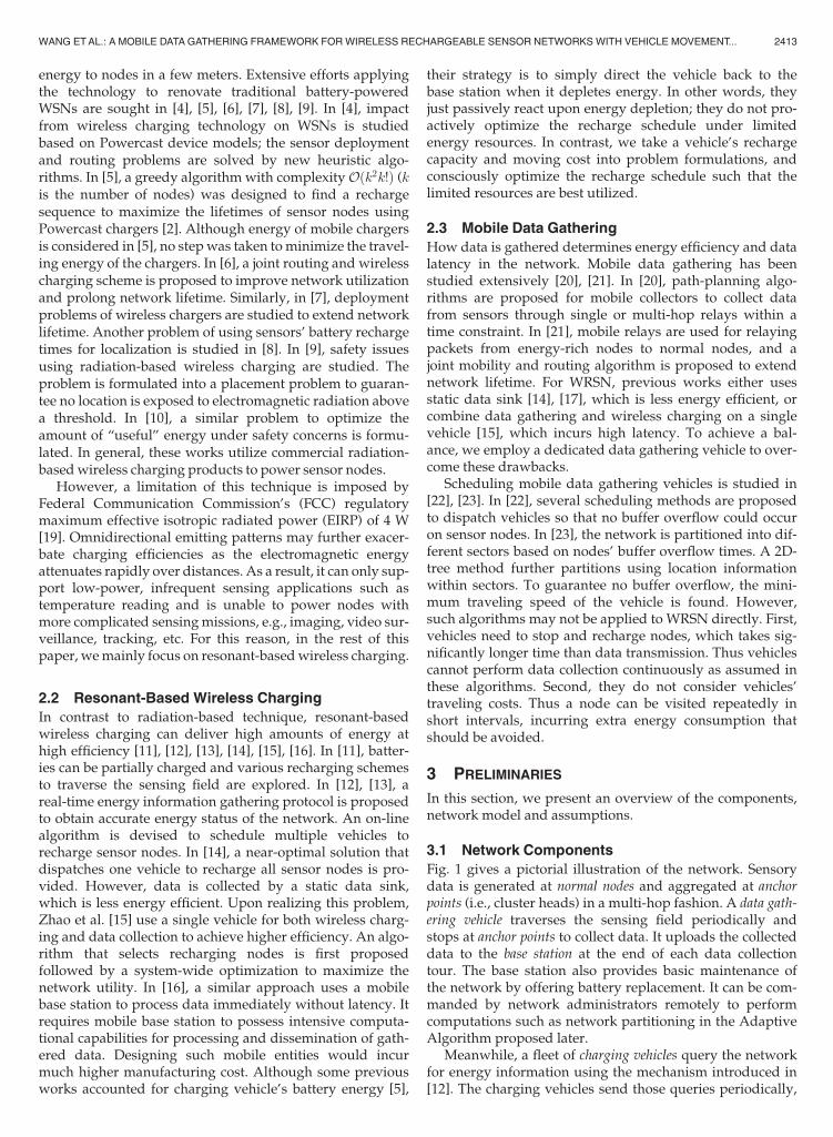
Fig. 1 gives a pictorial illustration of the network. Sensorydata is generated at normal nodes and aggregated at anchorpoints (i.e., cluster heads) in a multi-hop fashion. A data gath-ering vehicle traverses the sensing field periodically andstops at anchor points to collect data. It uploads the collecteddata to the base station at the end of each data collectiontour. The base station also provides basic maintenance ofthe network by offering battery replacement. It can be com-manded by network administrators remotely to performcomputations such as network partitioning in the AdaptiveAlgorithm proposed later.

Meanwhile, a fleet of charging vehicles query the networkfor energy information using the mechanism introduced in[12]. The charging vehicles send those queries periodically,

WANG ETAL.: A MOBILE DATAGATHERING FRAMEWORK FORWIRELESS RECHARGEABLE SENSOR NETWORKS WITH VEHICLE MOVEMENT... 2413

make recharge decisions (i.e., which nodes to recharge, inwhich order) and recharge nodes accordingly. Once acharging vehicle fulfills all requests, it sends out a query tosee whether there is new energy request. Both types ofvehicles return to the base station and have their own bat-teries replaced when their energy is low.

3.2 Network Model and Assumptions

We assume a number of Ns sensor nodes are uniformly ran-domly scattered in a square sensing field with side length L.

Node density of the network is r ¼ NsL2 . In this paper, we

focus on event-driven sensing applications and assumeevents occur at every location with equal probability, spa-tially and temporally independent of each other. Thus, thedata generation process can be modeled as a Poisson pro-cess with average rate � [26]. All sensors transmit at thesame power level with fixed transmission range dr. Theenergy consumed for transmitting/receiving a packet oflength l, denoted by et; er, is modeled as in [27], i.e.,et ¼ ðe1dar þ e0Þl, where e1 is the loss coefficient per bit, a isthe path loss exponent (usually from 2 to 4) and e0 is energyconsumed on sensing, coding, modulations. In this paper,

we use e0 ¼ 50� 10�8 J/bit, e1 ¼ 10� 10�8 J/bit, a ¼ 4.The network is split into a number c clusters. A cluster is

formed in a way such that the maximum hop count from anode to the anchor point (cluster head) is k. When a node fallswithin k-hops of multiple anchor points, it will join the clus-ter with the least number of hops. A data gathering vehiclestarts from the base station every Tc time period, stops atanchor point location i for time ti to gather all senseddata and returns to the base station after all anchor pointshave been visited. The dispatch interval Tc is greater thanthe duration of the data gathering tour. The data gatheringvehicle visits anchor point locations directly to minimizetransmission energy consumption on these nodes. Thetransmission bit rate is B.

There are also m charging vehicles working together toreplenish sensor batteries. A number of nodes are selectedfor a vehicle to form its recharge set. If a node cannot sur-vive the time needed to recharge all the other nodes in theset, it needs prioritized recharge (i.e., it should be charged ear-lier in the recharge sequence). Charging vehicles bring sen-sor batteries from zero to full capacity Cs in Tr time which isgoverned by battery characteristics (e.g., for a Panasonic Ni-

MH AAA battery [24] of battery capacity Cs = 780 mAhand Tr = 78 min.). All the vehicles are equipped with high-capacity batteries of Ch capacity and consume at ec J/mwhile moving at speed v m/s. In this paper, we have madethe following assumptions: 1) we assume the energy con-sumption during transmission and reception of a packet isequivalent (er � et); 2) the vehicles have positioning systemsand know their locations; 3) the locations of all the sensornodes are known to the vehicles (e.g., through a one-timeeffort during network initialization). Finally, importantnotations used in this paper are summarized in Table 1.

4 LOW LATENCY MOBILE DATA COLLECTION

IN WRSNS

We now study how to minimize data collection latencygiven k-hop clusters. To minimize delay, it is desirable tohave the data gathering vehicle stop at fewer anchor points.To ensure all data can be collected, the k-hop coverage areasof these anchor points should collectively cover the entirenetwork. The delay mainly depends on three variables: sumof stopping time at anchor points, traveling time through allanchor points and data uploading time to the base station.

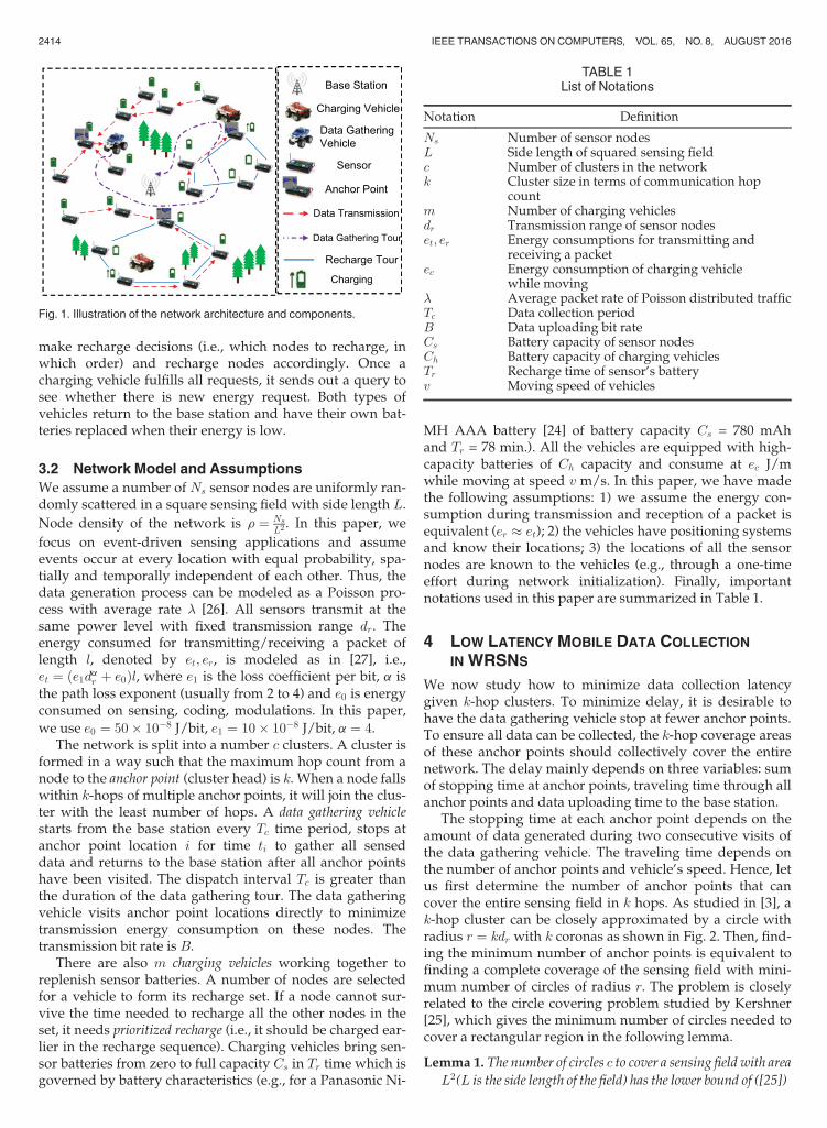
The stopping time at each anchor point depends on theamount of data generated during two consecutive visits ofthe data gathering vehicle. The traveling time depends onthe number of anchor points and vehicle’s speed. Hence, letus first determine the number of anchor points that cancover the entire sensing field in k hops. As studied in [3], ak-hop cluster can be closely approximated by a circle withradius r ¼ kdr with k coronas as shown in Fig. 2. Then, find-ing the minimum number of anchor points is equivalent tofinding a complete coverage of the sensing field with mini-mum number of circles of radius r. The problem is closelyrelated to the circle covering problem studied by Kershner[25], which gives the minimum number of circles needed tocover a rectangular region in the following lemma.

Lemma 1. The number of circles c to cover a sensing field with area

L2(L is the side length of the field) has the lower bound of ([25])

Fig. 1. Illustration of the network architecture and components.

TABLE 1List of Notations

Notation Definition

Ns Number of sensor nodesL Side length of squared sensing fieldc Number of clusters in the networkk Cluster size in terms of communication hop

countm Number of charging vehiclesdr Transmission range of sensor nodeset; er Energy consumptions for transmitting and

receiving a packetec Energy consumption of charging vehicle

while moving� Average packet rate of Poisson distributed trafficTc Data collection periodB Data uploading bit rateCs Battery capacity of sensor nodesCh Battery capacity of charging vehiclesTr Recharge time of sensor’s batteryv Moving speed of vehicles


c >2p

ffiffiffi3p ðL2 � 2pr2Þ

9pr2: (1)

Although the exact placement pattern to achieve thislower bound was not given in [25], it has been proved in[20] that the maximum coverage is achieved when we tes-sellate the sensing area with equilateral triangles of sidelength

ffiffiffi3p

kdr and place the centers of circles at the verticesof triangles. However, how to place these clusters in asquare sensing field considering the effects of boundarieswas not discussed in [20] so we introduce a placement pat-tern first. For a square sensing field with the origin (0,0) atthe left bottom, we place I circles parallel to the x-axis andJ circles parallel to the y-axis, then the cartesian coordinatesof centers of circles at the ith row, jth column are

½Xij; Yij� ¼½ ffiffiffi

3p ðj� 1Þr; 32 ði� 1Þr�i ¼ f2uþ 1;8u 2 Zg½ffiffi3p2 rþ ffiffiffi

3p ðj� 1Þr; 32 ði� 1Þr�

i ¼ f2u; 8u 2 Zg:

8>><>>: (2)

After the deployment pattern has been determined, thenumber of circles I to cover each row can be calculated as

I ¼bL32rc þ 1; L3

2r� bL3

2rc � 1

2

bL32rc þ 2; otherwise.

8<: (3)

The number of circles J to cover each column with an oddindex i ¼ f2uþ 1;8u 2 Zg is

J ¼ b Lffiffi3p

rc þ 1; Lffiffi

3p

r� b Lffiffi

3p

rc � 1

2

b Lffiffi3p

rc þ 2; otherwise.

((4)

The number of circles J to cover each column with an evenindex i ¼ f2u; 8u 2 Zg is

J ¼ b Lffiffi3p

rc; Lffiffi

3p

r� b Lffiffi

3p

rc ¼ 0

b Lffiffi3p

rc þ 1; otherwise.

((5)

Fig. 2 shows an example of equilateral triangular tessella-tion of 14 clusters covering a square sensing field with

k ¼ 3; L ¼ 3ffiffiffi3p

r. Compared to the lower bound of c > 7:97obtained from Eq. (1), an additional 6 clusters are needed tocover the boundaries of the field. Given a field length L, thenumber of clusters c (number of anchor points), coverage ofthe entire sensing field can be obtained from Eqs. (3), (4)and (5). Then we derive an upper bound of mobile datagathering latency in the following lemma.

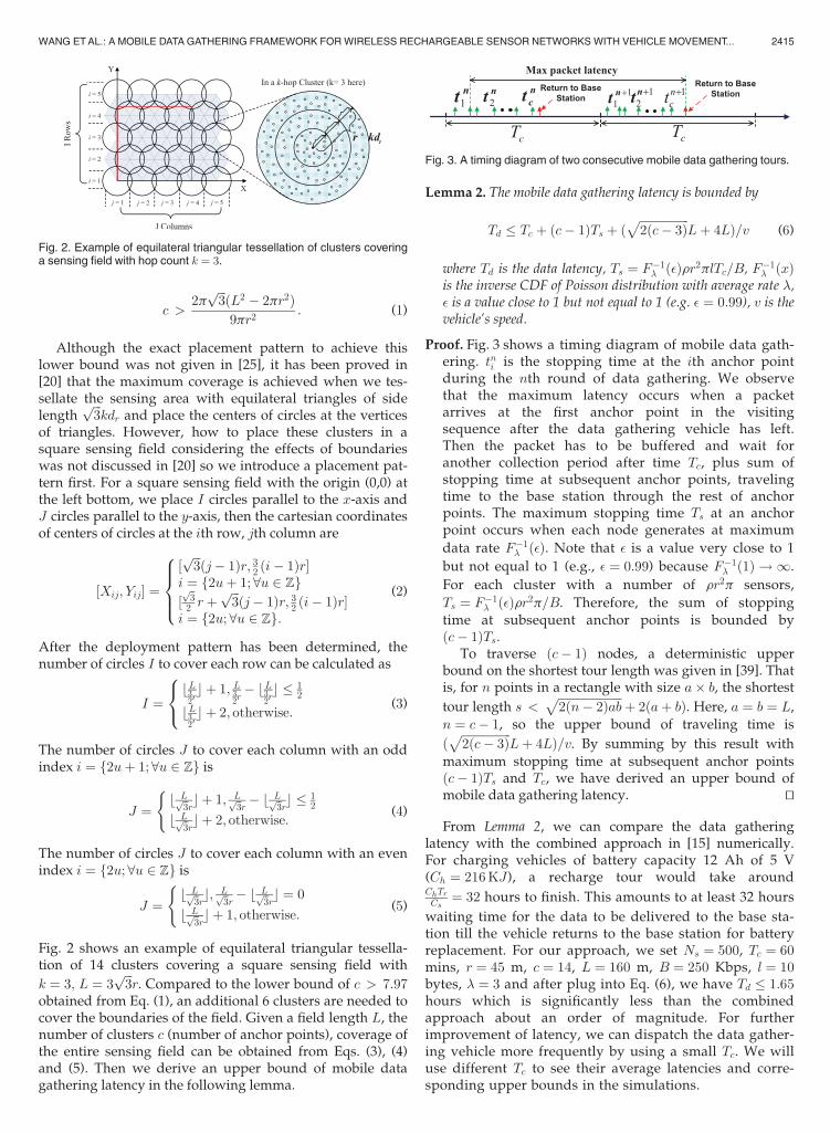
Lemma 2. The mobile data gathering latency is bounded by

Td � Tc þ ðc� 1ÞTs þ ðffiffiffiffiffiffiffiffiffiffiffiffiffiffiffiffiffi2ðc� 3Þ

pLþ 4LÞ=v (6)

where Td is the data latency, Ts ¼ F�1� ð�Þrr2plTc=B, F�1� ðxÞis the inverse CDF of Poisson distribution with average rate �,� is a value close to 1 but not equal to 1 (e.g. � ¼ 0:99), v is thevehicle’s speed.

Proof. Fig. 3 shows a timing diagram of mobile data gath-ering. tni is the stopping time at the ith anchor pointduring the nth round of data gathering. We observethat the maximum latency occurs when a packetarrives at the first anchor point in the visitingsequence after the data gathering vehicle has left.Then the packet has to be buffered and wait foranother collection period after time Tc, plus sum ofstopping time at subsequent anchor points, travelingtime to the base station through the rest of anchorpoints. The maximum stopping time Ts at an anchorpoint occurs when each node generates at maximum

data rate F�1� ð�Þ. Note that � is a value very close to 1

but not equal to 1 (e.g., � ¼ 0:99) because F�1� ð1Þ ! 1.

For each cluster with a number of rr2p sensors,

Ts ¼ F�1� ð�Þrr2p=B. Therefore, the sum of stoppingtime at subsequent anchor points is bounded byðc� 1ÞTs.

To traverse ðc� 1Þ nodes, a deterministic upperbound on the shortest tour length was given in [39]. Thatis, for n points in a rectangle with size a� b, the shortest

tour length s <ffiffiffiffiffiffiffiffiffiffiffiffiffiffiffiffiffiffiffiffiffiffi2ðn� 2Þabp þ 2ðaþ bÞ. Here, a ¼ b ¼ L,

n ¼ c� 1, so the upper bound of traveling time is

ð ffiffiffiffiffiffiffiffiffiffiffiffiffiffiffiffiffi2ðc� 3Þp

Lþ 4LÞ=v. By summing by this result with

maximum stopping time at subsequent anchor pointsðc� 1ÞTs and Tc, we have derived an upper bound ofmobile data gathering latency. tu

From Lemma 2, we can compare the data gatheringlatency with the combined approach in [15] numerically.For charging vehicles of battery capacity 12 Ah of 5 V(Ch ¼ 216KJ), a recharge tour would take aroundChTrCs¼ 32 hours to finish. This amounts to at least 32 hours

waiting time for the data to be delivered to the base sta-tion till the vehicle returns to the base station for batteryreplacement. For our approach, we set Ns ¼ 500, Tc ¼ 60mins, r ¼ 45 m, c ¼ 14, L ¼ 160 m, B ¼ 250 Kbps, l ¼ 10bytes, � ¼ 3 and after plug into Eq. (6), we have Td � 1:65hours which is significantly less than the combinedapproach about an order of magnitude. For furtherimprovement of latency, we can dispatch the data gather-ing vehicle more frequently by using a small Tc. We willuse different Tc to see their average latencies and corre-sponding upper bounds in the simulations.

Fig. 2. Example of equilateral triangular tessellation of clusters coveringa sensing field with hop count k ¼ 3.

Fig. 3. A timing diagram of two consecutive mobile data gathering tours.


5 NUMBER OF CHARGING VEHICLES FOR k-HOP

WRSN

Having discussed k-hop cluster formation and datalatency in our framework, we now analyze the minimumnumber of charging vehicles needed to fulfill all energyrequests given the number of clusters c obtained fromEqs. (3), (4), (5).

5.1 Number of Charging Vehicles

In an earlier work [12], we have proposed the energy neu-tral condition that must hold in a long time period for theperpetual operation of the network,

EðT Þ � RðT Þ þ E0 (7)

in which T is a large time, EðT Þ is the total energy con-sumption of the network up to T , RðT Þ is the total energyreplenished into the network by the charging vehicles upto T and E0 is the initial energy of all the sensor nodes.The energy neutral condition states that the energy con-sumption of all the sensor nodes must be less than orequal to the total energy available in long term. Other-wise, sensor nodes would eventually deplete energy.Note that for the network to function, it is not necessaryfor the condition to hold at every single moment. In prac-tice, a small fraction of the network may consume moreenergy in a short time window due to external activities,leading to temporary unbalance between energy con-sumption and replenishment. As long as there are enoughcharging vehicles, these nodes will be recharged, andsuch unbalance is transient, not permanent.

Our objective is to obtain the minimum number of charg-ing vehicles m needed for Eq. (7) to hold. First, we estimateRðT Þ which is the amount of energy that can be replenishedinto the network. The maximum recharge capacity of acharging vehicle is achieved when it recharges sensor nodescontinuously without any idling time. The longest recharg-ing time for a sensor occurs when a node’s energy isbrought from zero energy to full capacity which takes Tr

time plus the longest moving time between two consecutivesensors in the recharge sequence (moving on the diagonalof the square sensing field). Therefore, in the worst scenario,

it takesffiffiffi2p

L=vþ Tr time to recharge each sensor. Then wecan estimate the energy replenished into the network in Ttime bym charging vehicles,

RðT Þ ¼ mCbTffiffiffi2p

L=vþ Tr

: (8)

Next, we need to derive EðT Þ on the left hand side ofEq. (7) which is a random variable. Given the structure ofthe cluster of radius r ¼ kdr, each corona carries traffic loadsfrom all outer coronas. The number of nodes in the ith

corona, is Ni ¼ ð2i� 1Þd2rpr for 0 < i � k. Since the out-most kth corona only needs to send out its own data anddata is generated independently, the mean of energy con-sumption at the kth corona mk in time period T is,

mk ¼ Ni�Tet ¼ ð2k� 1Þd2rpr�Tet: (9)

For the ith corona (0 < i < k), it carries all the traffic fromthe outer coronas so the mean energy consumption is,

mi ¼ Ni�Tet þXkj¼iþ1

Nj�T ðet þ erÞ

¼ d2rpr�T�ðk2 � i2Þðet þ erÞ þ ð2i� 1Þet

�:

(10)

Then we can compute the mean of network energy con-sumptions EðT Þ,

EðT Þ ¼�Xk�1

i¼1

�ðk2 � i2Þðet þ erÞ þ ð2i� 1Þet�

þ ð2k� 1Þet þ k2ðet þ erÞ�d2rpr�Tc

¼ 2

3k3 � 1

2k2 � 1

6k

� �ðet þ erÞ þ k2et

� �d2rpr�Tc:

(11)

Based on the energy neutral condition, by combiningRðT Þ inEq. (8) andEðT Þ in Eq. (11), we have the following lemma.

Lemma 3. The probability for the energy neutral condition tohold is

Pop ¼ FRðT Þ þ E0 � EðT Þffiffiffiffiffiffiffiffiffiffiffi

EðT Þq

0B@

1CA; (12)

where RðT Þ and EðT Þ are obtained in Eq. (8) and Eq. (11),respectively. Fð�Þ denotes the Cumulative Distribution Func-tion of the Normal distribution.

Proof. Energy consumption of a cluster can be described bythe sum of independent Poisson variables over T . WhenT is observed over a long time period, we can use theCentral Limit Theorem to approximate Poisson distribu-

tion by a Normal distribution NðEðT Þ; EðT ÞÞ(the meanand variance of a Poisson distribution is the same) [29]. tuFrom Lemma 3, we immediately get the following

Proposition.

Proposition 1. The minimum number of charging vehiclesrequired to achieve perpetual operation is

m ¼ðF�1ð�Þ

ffiffiffiffiffiffiffiffiffiffiffiEðT Þ

qþ EðT Þ � E0Þð

ffiffiffi2p

L=vþ TrÞCsT

2666

3777; (13)

whereF�1ð�Þ is the inverse cumulative distribution function ofNormal distribution, � is a value very close to 1 but not equalto 1.

Proof. Since F�1ð1Þ ! 1, we consider the networkachieves perpetual operation with very high probability

approaches 1 but not equal to 1, e.g., � ¼ 0:99;F�1

ð0:99Þ � 2:33. From Eq. (12), we have

mCbTffiffi2p

L=vþTr þ E0 � EðT ÞffiffiffiffiffiffiffiffiffiffiffiEðT Þ

q 2:33;


after some manipulations we can obtain the minimumnumber of charging vehicles m needed to satisfy theenergy neutral condition. tuBased on the results from Proposition 1 and Lemma 2, we

demonstrate the trade-off between number of chargingvehicles and data latency. For L ¼ 400 m, we change thenumber of cluster hop count k and plot the correspondingnumber of vehicles needed as well as upper bound of datalatency in Fig. 4. We can see a trade-off point around k ¼ 3.It means when k ¼ 3, we can minimize the number of charg-ing vehicles without sacrificing too much from the data col-lection latency.

5.2 Estimate Node Lifetime

To devise effective recharging schedules, we need to knowhow long a sensor node can survive after it has requestedfor recharge. Such information is vital in making rechargedecisions in the next section. Since a node’s energy con-sumption rate is a random variable and depends on trafficpatterns, it is important for each node to know its trafficburden which is determined by the number of hops frombase station. This information can be obtained by messagepropagation from the base station in various routing proto-cols and adjusted accordingly during operation.

From Eqs. (9) and (10), we know the average traffic rateof a node in the jth corona (1 � j � k) is, �j ¼ �ð1þ ðk2�j2Þ=ð2j� 1ÞÞ. Given residual energy Er, the maximum num-

ber of packets the node can transmit is n ¼ b ErðetþerÞc.

Lemma 4. Given a recharge sequence of N nodes in which a nodeat the jth corona waiting to be recharged, it will survive time twith probability (lifetime Lj > t),

P ðLj > tÞ ¼ 1� gðN;�jtÞGðNÞ ; (14)

where gð�; �Þ and Gð�Þ are the lower incomplete gamma functionand complete gamma function[29], respectively.

Proof. Since sensor nodes are randomly deployed in thefield, and the data generation process is independent ofeach other, the summation of packet interarrival timesuntil the sensor node can no longer transmit packets isthe lifetime of the sensor node. Because data generationis Poisson distributed with rate �j, the interarrival time

of packets is exponentially distributed. It is known thatthe sum of independently identically distributed expo-nential variables results a Gamma distribution with proba-bility density function

fLjðxÞ ¼ �je

��jx ð�jxÞN�1ðN � 1Þ! ; x 0; (15)

and the Cumulative Distribution Function of Gammadistribution is

P ðx < tÞ ¼Z t

0

�je��jx ð�jxÞN�1ðN � 1Þ! dx ¼

gðN; �jtÞGðNÞ : (16)

tuProposition 2. For the recharge sequence of N nodes, if a node at

the jth corona has probabilitygðN;�jTlÞ

GðNÞ � 0, Tl ¼ ðN � 1ÞðTrþffiffiffi2p

L=vÞ, no matter where the node is placed in the rechargesequence, it will not deplete battery energy before its recharg-ing starts.

Proof. The worst case occurs when the node is placed atthe end of the recharge sequence. The longest waitingtime to get recharged is Tl ¼ NTr þ ðN � 1Þ ffiffiffi

2p

L=v

since there areN � 1 nodes ahead withffiffiffi2p

L=vmaximum

traveling time between two sensor nodes andffiffiffi2p

L is

the diagonal of the square field. OncegðN;�jTlÞ

GðNÞ � 0,

P ðLj > TlÞ approaches probability 1 so it is guaranteedto recharge the node before it depletes battery energy. tuBased on Proposition 2, given a recharge sequence, we can

calculate the possibility that a node can survive the entirerecharging process. This lays the theoretical foundations tosolve the recharge scheduling problem in the next section.

5.3 Adaptive Recharge Threshold

We observe that the difference of energy consumptionsbetween nodes at different locations is mainly caused bydata communications. Although the hop count for clusters kshould not be too large to avoid the energy hole problem onanchor points, it is inevitable to have higher data traffic inthe inner coronas. If all the nodes follows a universallysame recharge threshold, it may result some nodes close tothe anchor point nodes to deplete energy very soon andlead to unfair service for nodes with higher consumptionrates. To this end, the recharge thresholds should be madeadaptive and proportional to energy consumption rates atdifferent coronas. In other words, nodes closer to the anchorpoints should request recharge more frequently than others.

Let tið0 < tj < 1Þ denote the recharge thresholds fornodes at the jth corona. We make the ratio between therecharge thresholds of corona i and j equal to that betweentheir energy consumptions due to data transmission.Assume we have set the recharge threshold of the firstcorona to be t1. The thresholds for other coronas are,

ti ¼ ðk2 � i2Þðet þ erÞ þ etð2i� 1Þðk2 � 1Þðet þ erÞ þ et

t1 � 2k2 � ði� 1Þ2 � i2

2k2 � 1;

(17)

Fig. 4. Trade-off between number of charging vehicles and data collec-tion latency.


where 0 < i < k. The approximation is taken under theassumption that et � er. To illustrate Eq. (17), e.g., k ¼ 5,

after t1 is set, we obtain t2 ¼ 4549 t1, t3 ¼ 37

49 t1, t4 ¼ 2549 t1 and

t5 ¼ 949 t1.

6 CAPACITATED MULTI-VEHICLE RECHARGE

PROBLEM WITH BATTERY DEADLINES

During operation, the charging vehicles query sensors forrecharge and they usually engage in multiple recharge tasksat different locations. In this section, we study a CapacitatedMulti-Vehicle Recharge Problem with Battery Deadlines(CaMP-BaD) and consider practical constraints from realsensing applications. The first challenge is the constantchanges (i.e., decrease) of charging vehicles’ energy due tomoving and recharging sensor nodes. The recharge routeshould be planned carefully to reflect charging vehicles’scurrent energy status and traveling costs to nodes’ locations.The second challenge is the nonuniform energy consump-tion due to data transmissions. Some nodes consume energyat higher rates and should be taken care of more frequentlythan others to maintain the functionality of the network. Therecharge routes should reflect all aforementioned concerns.The difficulty of the problem lies in achieving conflictinggoals—the need to keep the whole network running pushesthe charging vehicles to recharge as many sensor nodes aspossible while the desire to reduce cost means that chargingvehicles should minimize traveling distances to save energycost. Therefore, an ideal solution should achieve a good bal-ance between the twowithout sacrificing either.

Next we show the recharge problem can be formulatedinto a Profitable Traveling Salesmen Problem with Capacity andBattery Deadline constraints (PTSP). In the Profitable Travel-ing Salesmen Problem [30], a reward is collected by visitinga city while the objective is to maximize the profit which isdefined as the reward minus cost. In our problem, thereward represents the amount of energy that can be replen-ished into a sensor node and the cost measures the energycost in traveling to that node’s location.

To tackle the problem, we first present a straightforwardGreedy Algorithm. After realizing that the greedy algorithmmight incur extra movements of charging vehicles, we fur-ther propose a three-step Adaptive Algorithm through 1)adaptive network partition using K-means algorithm, 2)Capacitated Minimum Spanning Tree (CMST) formationand 3) route improvements using node insertions. By parti-tioning the network, the charging vehicles are confined intheir own regions so traveling back and forth through theentire field is avoided. Then we form CMST for each charg-ing vehicle. The trees indicate which subset of sensor nodesthe charging vehicle should select to minimize travelingcost and ensure the total weight of the tree is within thecharging vehicle’s recharge capacity. After that, we performroute improvements on nodes in CMST to capture sensornodes’ dynamic battery deadlines. Finally, we analyze thecomplexity of the proposed algorithms.

6.1 Problem Formulation

The recharge optimization problem can be defined as fol-lows. Given a set of charging vehicles S ¼ f1; 2; . . . ;mg and

a set of recharge node list N ¼ f1; 2; . . . ; ng, we formulatethe CaMP-BaD problem into a PTSP problem. Consider agraph G ¼ ðV;EÞ, where Vi (i 2 N ) is the location of sensornode i to be visited, and E is the set of edges. We add a ver-tex V a

0 as the starting position of vehicle a. Each edge Eij isassociated with a traveling energy cost cij, which is propor-tional to the distance between nodes i and j, ca0i representsthe cost from initial position V a

0 of vehicle a to node i. Acharging vehicle a has recharge capacity Ca (� Ch) thatdetermines the maximum number of nodes it can rechargebefore it goes back to the base station for its own batteryreplacement. Different charging vehicles might have differ-ent recharge capacities during the run. Each sensor node ihas lifetime Li and demand (reward) for energy recharge ri(demand equals the total battery capacity of a sensor nodeminus its residual energy). Ai specifies the arrival time for avehicle at sensor node i.

We introduce two decision variables xaij for edge Eij and

yia for vertex Vi. The decision variable xaij is 1 if an edge is

visited by vehicle a, otherwise it is 0. The decision variableyia is 1 if and only if node i is served by vehicle a, otherwiseit is 0. ui is the position of vertex i in the path. Our objectiveis to maximize the total amount of energy recharged minustotal traveling energy cost of the charging vehicles whileensuring the recharge capacities of charging vehicles are notexceeded and no sensor node depletes battery energy

P1 : maxXma¼1

Xni¼1

riyia �Xma¼1

Xni¼1

Xnj¼1

cijxaij �

Xma¼1

Xni¼1

ca0ixa0i

( ):

(18)

Subject toXnj¼1

xa0j ¼ 1; a 2 S (19)

Xni¼1

xik ¼Xnj¼1

xkj ¼ 1; k 2 N (20)

Xni¼1

riyia þXni¼1

Xnj¼1

cijxaij þ

Xni¼1

ca0ixa0i � Ca; a 2 S (21)

Xma¼1

yia ¼ 1; i 2 N (22)

Ai � Li; i 2 N (23)

xaij 2 f0; 1g; i; j 2 N ; a 2 S (24)

yia 2 f0; 1g; i 2 N ; a 2 S (25)

1 � ui � nr; i 2 N (26)

ui � uj þ ðnr �mÞxij � nr �m� 1; i; j 2 N ; i 6¼ j: (27)

In the above formulation, constraint (19) states that therecharge tour for each charging vehicle starts at initial posi-tion 0. Constraint (20) ensures the connectivity of the pathand every vertex is visited at most once. Constraints (21)and (22) guarantee the vehicle’s capacity is not violated andeach vertex is visited by only one charging vehicle. Con-straint (23) guarantees the arrival time of the charging vehi-cle is within each sensor’s residual lifetime. Constraints (24)


and (25) impose xij and yia to be 0-1 valued. Constraints (26)and (27) eliminate the subtour in the planned route, whichis formulated according to [31]. The classic TSP with Profitscan be considered as a special case of CaMP-BaD withunlimited capacity and unspecified deadlines. Since TSPwith Profits is well known to be NP-hard [30], CaMP-BaD isalso NP-hard.

A direct solution to the CaMP-BaD is difficult to obtainand rare in existing literature. Hence, we review some liter-ature that has partially solved the problem. In [32], a surveyof different approaches to TSP with profits is presented.Lagrangian decomposition method and approximated algo-rithms developed based on existing solutions can providesolutions very close to optimality. However, adding capac-ity (Eq. (21)) and time (Eq. (23)) constraints makes the prob-lem more complicated. A great deal of research efforts onthese two constraints are devoted in the context of VehicleRouting Problem, in which a number of vehicles start froma depot to visit client locations and the objective is to mini-mize the total traveling cost of the vehicles. In [35], theCapacitated Vehicle Routing Problem where each vehiclehas a fixed capacity is considered. Time constraints arestudied in Vehicle Routing Problem with Time Windows[33]. A local search algorithm is proposed in [33] based onthe k-exchange concept, and reduction of the computationfor checking feasibility constraint is also studied. A theoreti-cal approach to obtaining 3logn-approximation algorithm issought in [34] (n is the number of nodes). However, subrou-tines from existing solutions visit the node with the smallestdeadline last, which contradicts to our problem where suchnodes should be serviced earlier.

Due to the nature of our problem, it is not realistic to usestandard optimization techniques [32], [35] because thesemethods deal with datasets of static inputs and the optimi-zation is usually done offline through a one-time effort. Incontrast, energy consumption in our framework is probabi-listic in nature. A charging vehicle’s recharge capacitydeclines after recharging sensor nodes, so the input to ourproblem is more dynamic than that most existing solutionshave considered. Furthermore, existing algorithms requirehigh computation power that may not be available oncharging vehicles. Therefore, we need to design algorithmssuitable to our problem context. Next, we present two suchalgorithms.

6.2 Greedy Algorithm

The simplest approach is a greedy algorithm which selectsthe node with the maximal recharge profit (i.e., rechargereward less traveling cost) for each node selection. After acharging vehicle finishes recharging a node, it picks thenext available node with the maximal profit. When thecharging vehicle’s energy falls below a threshold x, itreturns to the base station for battery replacement and thenresumes recharge in the same fashion.

Despite of its simplicity, GA may have some problems inpractice. The first problem is that the charging vehicle mightmove back and forth over long distances, thereby increasingthe traveling energy cost. This happens when the node withthe maximum profit lies faraway, and the energy efficiencyof charging vehicles can deteriorate. Second, because the

only consideration is profit, it may not fulfill a rechargerequest in a fixed time. These observations offer us roomfor further improvements. To prevent charging vehiclesfrom traveling long distances, we can confine the scope ofmovements by partitioning the network into several regionsadaptively and assigning each charging vehicle to one ofthe regions. Second, a more sophisticated schedulingmethod should be developed to capture charging vehicles’capacity as well as sensors’ battery deadline constraints. Inthe next subsection, we will introduce an Adaptive Algo-rithm to address the limitations in GA.

6.3 Recharge by Adaptive Algorithm

6.3.1 Adaptive Network Partitioning

In the first step, the base station requests sensor nodes forenergy information periodically using the method in [12].Then it adaptively partitions the network into m regionsaccording to the originating locations of requests. The resultof partitions is disseminated to the charging vehicles usinglong range radio. We utilize the well-known K-means algo-rithm to perform the partition [36]. Using the K-means algo-rithm would allow the charging vehicles to adaptivelyselect a subset of nodes with their square sum of distanceminimized regarding to the centroid of each region so thecharging vehicle would only move in a confined scope, andmost likely with less distances. For each region, our objec-tive is to minimize the intra-region square sum of inter-node distance

S ¼Xmj¼1

Xnri¼1knðjÞi � mðjÞk2 (28)

in which knðjÞi � mðjÞk2 is the square distance between a

recharge node ni of region j to the region’s centroid mðjÞ

(computed by taking the mean of x; y coordinates of all thenodes in the region). Now we briefly explain the partition-ing process.

Initially, we select a number of m sensor nodes with theminimum lifetime from N to be the centroid of regions. Weassign each node to the closest centroid. After all the nodeshave been associated with a centroid, we re-calculate cen-troid positions taking the average value of x and y coordi-nates of nodes in the region. This process is repeated untilthe centroids no longer change. After the partition, the cen-troid of each region represents a virtual position that hasthe minimal sum of distances to all the nodes in its region.This position can be used as the starting position for thecharging vehicle to recharge nodes in its region.

6.3.2 Generating Capacitated Minimum Spanning Tree

In the first step, m regions are generated and each chargingvehicle only needs to take care of the nodes in its region. Todecide the route to recharge sensor nodes, we need toensure each charging vehicle’s recharge capacity is notexceeded (Eq. (21)). At the same time, we also want to mini-mize the traveling energy cost for the charging vehicle.These requirements lead to finding Capacitated MinimumSpanning Tree (CMST)[37] where the total sum of demandsfrom nodes does not exceed the charging vehicle’s capacityand the minimum traveling energy cost can be found by


constructing the minimum spanning tree. In this way, wecan ensure sensor nodes close to each other are placed inthe same tree and later covered by the same recharge route.

The exact solution to CMST requires us to go over allpossible tree setups and pick the one with the lowest cost,which involves exponential computation. Fortunately, anefficient algorithm by Esau-Williams (EW) can find a subop-timal solution very close to the exact solution in polynomialtime [37]. The EW algorithm merges any two subtrees whenthere is a “saving” in the total cost of two trees.

Nevertheless, there are some limitations of the originalEW algorithm when applied for our problem. First, whendetermining whether two subtrees can be merged, only thedemands from sensor nodes are counted whereas the travel-ing costs on edges are not considered. Second, multiple suchtrees can be generated. How does the charging vehicledecide which tree to pick? To overcome these limitations, weextend the original EW algorithm. As mentioned earlier, adeterministic upper bound on the shortest tour length isdeveloped as

ffiffiffiffiffiffiffiffiffiffiffiffiffiffiffiffiffiffiffiffiffiffi2ðn� 2Þabp þ 2ðaþ bÞ for a rectangle of side

length a, b and n nodes. For the square sensing field with Lside length and subtree of nb nodes, we have a loose upper

bound on the traveling cost, ð ffiffiffiffiffiffiffiffiffiffiffiffiffiffiffiffiffiffiffi2ðnb � 2Þp þ 2ÞLec. Second,

whenmultiple trees are generated, we select a tree that maxi-mizes the ratio of total energy demand to traveling cost. Inthis way, we can exploit limited resources on chargingvehicles better and improve energy efficiency of the network.

Next, we explain our extension to the EW algorithm indetail. Each charging vehicle computes CMST indepen-dently by iteratively updating a distance matrix. The dis-tance matrix facilitates the computation process bymaintaining costs of tree nodes. Let us denote recharge set

N a with na nodes for charging vehicle a (S m

a¼1N a ¼ N r).

We define trade-off function ti for each node in its recharge

set N a, ti ¼ minðcðaÞij Þ � cðaÞ0i and j 2 Pi, where Pi is the neigh-

boring set of node i, minðcðaÞij Þ finds the minimum cost from

node i to its neighbor j in Pi and cðaÞ0i is the cost from node i

to charging vehicle’s starting position (i.e., the root).1 Thetrade-off function evaluates whether it is beneficial to mergesubtrees of nodes i and j. A positive ti indicates that itincurs smaller cost for the charging vehicle to directly travelfrom the root to node i so merging subtrees of nodes i and jis not preferred. A negative ti indicates how much it can besaved by connecting subtrees of i and j. Thus the most nega-tive ti results in the most savings in an iteration.

After ti has been computed, we search through all trade-offs tið8i ¼ 1; . . . ; na), looking for the minimum trade-off(i.e., the most negative value). Assume tk is the most nega-tive trade-off and j is k’s minimum cost neighbor. To cap-ture charging vehicle’s capacity constraint in Eq. (21), if thesum of total demands from the subtrees of k and j plusupper bound of their traveling cost is less than the rechargecapacity (which means we can cover the subtrees of k and junder the current recharge capacity), we merge the subtreesof k and j. Since the action of merging k and j has resultedin a lower total traveling cost to k, direct traveling from the

root to reach k has higher cost and should be avoid. So we

remove the edge from node k to the root by setting cðaÞ0k in

the distance matrix to1.At this point, two subtrees satisfying the recharge capacity

with minimum sum of cost have been merged, and we needto update the minimum cost of the newly merged tree to theroot. It is done by updating the minimum cost in the distancematrix from the tree to the root by setting the value to

minðcðaÞ0i Þ, where i is the node in the newlymerged tree.On the other hand, if merging subtrees of k and j violates

charging vehicle’s recharge capacity, we need to restrict anyfurther actions to merge j to k because these two trees can-not be covered by the charging vehicle in a single run. Thenwe recompute the trade-off function tk to search for the nextneighboring node that results in minimum trade-off untilthe next valid neighboring node j is found and merged tothe existing trees. The iteration continues until all the trade-offs become nonnegative, in other words, no more savingcan be made.

After the CMST has been generated, the charging vehicleselects a tree with the maximal ratio of recharge demand tosum of tree’s edge cost and utilizes the route improvementalgorithm to form the final recharge sequence among thetree nodes. After the charging vehicle finishes rechargingnodes in a tree, it checks whether its energy falls below athreshold. If so, it returns to the base station for batteryreplacement. Table 2 shows the pseudo-code of ourextended EW algorithm.

6.3.3 Insertion Algorithm for Route Improvement

After the CMST has been obtained, next we want to producea recharge sequence for nodes such that for each node thecharging vehicle arrives before its battery deadline. Let usdenote the result from CMST to be a recharge node set N ðaÞr

TABLE 2Extended Esau-Williams Algorithm

input: recharging node setN r, distance matrix DðaÞ,recharge capacity Ca, demand of nodes di, i 2 N a.output: CMST nodes need to recharge.

Initialize tðaÞ < 0, weight of tree, CðaÞ ¼ 0.while (tðaÞ < 0)Find neighbormi of i results min cost,min

mi

DðaÞði;miÞ.Compute trade-off value list t

ðaÞi ¼ DðaÞði;miÞ �DðaÞð1; iÞ.

Find k and j resulting most negative trade-off value,

k miniðtðaÞÞ; j mk:

doAdd new nodesNnew kþ j if not exist in current treesifweight of merging subtree of Nnew < Ca

Add Nnew to corresponding tree iUpdate cumulative weight of corresponding tree i, C

ðaÞi .

Declare Nnew is accepted.elseupdate DðaÞðk; jÞ 1Search for next min cost neighbor for k,

mk minmk

DðaÞðk;mkÞ.Recompute trade-off for k, t

ðaÞk ¼ DðaÞðk;mkÞ �DðaÞð1; kÞ.

Declare Nnew rejected.until (Nnew is accepted) or (all t

ðaÞi 0)

end whileSelect a tree results maximum energy efficiency.

1. In order to reduce intra-region traveling cost, we set the centroidoutput from K-means algorithm to be the root.


(N ðaÞr N a). Recall that if the condition in Proposition 2 issatisfied, a node can be placed anywhere in the recharge

sequence. We call such a set of nodes a feasible node set N ðaÞf .

Otherwise, a node may need prioritized treatment to meetits battery deadline. We denote such a set of nodes as a pri-

oritized setN ðaÞp (N ðaÞf [ N ðaÞp ¼ N ðaÞr ).

Intuitively, we first use a Traveling Salesman Problemalgorithm (e.g., the Oðn2Þ nearest neighbor heuristic algo-rithm [38], where n is the number of nodes) to find a feasiblesolution as the initial sequence C for nodes in the feasible

set N ðaÞf . Then we insert nodes from the prioritized set N ðaÞp

into C while ensuring the battery deadline in Eq. (23) for all

nodes are still met. To this end, we sort the nodes in N ðaÞp in

a descending order of residual lifetimes and denote thesorted sequence as V. We insert these nodes starting fromthe first node V1. Let Ai denote the arrival time of the charg-ing vehicle at the ith node in the shortest path C,

i ¼ f1; 2; . . . ; nðaÞf g.To insert the jth node Vj from V into C, we first find

positionmt inC such that Amt � lVjand Amtþ1 > lVj

where

lVjis Vj’s lifetime. We call mt the temporary maximum posi-

tion to insert Vj. It indicates the maximum number of nodesin C that can be served before node Vj depletes its battery.To accommodate the remaining jVj � j nodes, we need tofind a position such that even all the remaining nodes areinserted before Vj, Vj can still meet its battery deadline. Wefind the maximum position m such that Am � Amt�Pnap

i¼jþ1 ti and Amþ1 > Amt �Pnap

i¼jþ1 ti, where ti is the

recharge time of Vj. Now, the maximum position m repre-sents the rightmost position Vj can be inserted if all remain-ing nodes are later inserted before Vj.

For each of the m possible positions that Vj can beinserted, a total traveling cost is computed and the one that

minimizes the traveling cost is selected as the final insertionposition for Vj. Then we obtain a new sequence C andremove Vj from V. The iteration continues until we exhaustV or an infeasible situation is encountered. Table 3 showsthe pseudo-code of the insertion algorithm.

We briefly illustrate how the insertion algorithm worksin Fig. 5. We consider two nodes V1, V2 with lifetime 104and 90 mins that need to be inserted into a feasible rechargesequence. We find the position k to insert V1 is betweennode 6 and 7 since A6 < lV1

< A7. To ensure V1 can sur-

vive when V2 is later inserted before V1, k0 can only be

between node 3 and 4 (since A3 < A6 � TV1< A4). Then

we search all the four possible locations (before node 1, 2, 3,4) and find that the position before node 3 minimizes thetraveling cost. Thus V1 is inserted between node 2 and 3.We repeat the procedure for V2. Since it is the last node, wecan directly calculate the rightmost insertion position k0 andfind the minimum cost among possible inserting positions.

Remarks. Due to the randomness in sensors’ lifetimes, itis very difficult to derive a theoretic performance bound ofthe algorithm. However, we have conducted simulations inSection 7.1 and find our algorithm has about 1.06 approxi-mation ratio to the optimal solution.

6.4 Complexity Analysis

We now analyze the complexity of our algorithms. The com-plexity of the greedy algorithm is OðnÞ because it onlyselects the maximum profitable node at each step. For theadaptive algorithm, the base station has abundant resourcesand it performs the k-means algorithm. So we focus on thecomputing burdens on charging vehicles for calculatingCMST and route improvements. In the worst case, there isonly one charging vehicle to recharge n nodes. For theextended EW algorithm, finding the minimum trade-off

value requires n2 þ 2n iterations at the outer loop. In theinner loop, the worst case is that for a node with the mini-mum trade-off value, every minimum-cost neighbor isrejected due to capacity violations. So n iterations are

required. In sum, its time complexity is Oðn3Þ.For the route improvement algorithm, running a TSP

algorithm requires Oðn2Þ time. Sorting nodes’ lifetimes

requires Oðn log nÞ time. Then, insertion requires Oðn2Þ

TABLE 3Insertion Algorithm

input: CMSTN ðaÞr , lifetime li and recharge time ti, i 2 N ðaÞr ,

distance matrixDðaÞ, feasible setN ðaÞf satisfying Proposition 2.output: resultant recharge sequenceC.Compute shortest path in the feasible set,C TSP(N ðaÞf )

Sort N ðaÞp in a descending order of lifetime as VInitialize i 1, last step node position k 1.while V 6¼ ;Find temporary max positionmt inC such thatAmt � lVi

and Amtþ1 > lVi

Find the max insertion positionm such that

Am � Amt �Pn

pr

k¼iþ1 tk and Amþ1 > Amt �Pn

pr

k¼iþ1 tk.if Cannot findm 0. break,return infeasible and report.endifSet minimum cost cmin 1:for x from 0 tomInsert node Vi intoC, get temporary sequenceCt

Calculate cost c PjCtj�1j¼1 Daðj; jþ 1Þ:

if c < cmin,C Ct, cmin c, k x. end ifend fori iþ 1, update V V� iend whileReturn recharge sequenceC, minimum cost cmin.

Fig. 5. Illustration of insertion algorithm.


time. Hence, the total time complexity of route improve-

ment algorithm is Oðn2Þ and the adaptive algorithm takes

Oðn3Þ time. Note that although the proposed algorithms arecentralized, they run on the charging vehicles that usuallyhave much higher computation and energy resources thancommon sensor nodes. It is not difficult for them to handlecomputations for large networks.

6.5 An Example of Algorithms

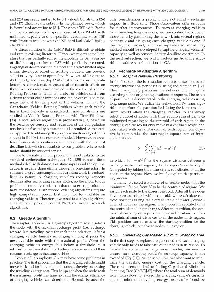
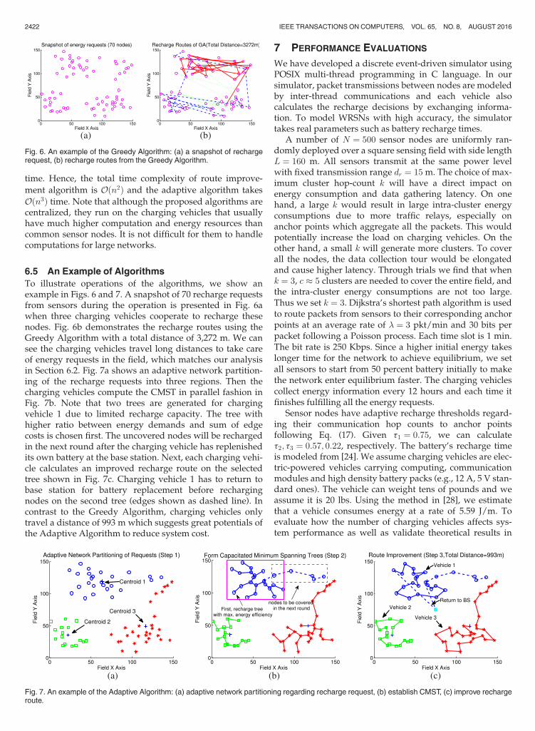
To illustrate operations of the algorithms, we show anexample in Figs. 6 and 7. A snapshot of 70 recharge requestsfrom sensors during the operation is presented in Fig. 6awhen three charging vehicles cooperate to recharge thesenodes. Fig. 6b demonstrates the recharge routes using theGreedy Algorithm with a total distance of 3,272 m. We cansee the charging vehicles travel long distances to take careof energy requests in the field, which matches our analysisin Section 6.2. Fig. 7a shows an adaptive network partition-ing of the recharge requests into three regions. Then thecharging vehicles compute the CMST in parallel fashion inFig. 7b. Note that two trees are generated for chargingvehicle 1 due to limited recharge capacity. The tree withhigher ratio between energy demands and sum of edgecosts is chosen first. The uncovered nodes will be rechargedin the next round after the charging vehicle has replenishedits own battery at the base station. Next, each charging vehi-cle calculates an improved recharge route on the selectedtree shown in Fig. 7c. Charging vehicle 1 has to return tobase station for battery replacement before rechargingnodes on the second tree (edges shown as dashed line). Incontrast to the Greedy Algorithm, charging vehicles onlytravel a distance of 993 m which suggests great potentials ofthe Adaptive Algorithm to reduce system cost.

7 PERFORMANCE EVALUATIONS

We have developed a discrete event-driven simulator usingPOSIX multi-thread programming in C language. In oursimulator, packet transmissions between nodes are modeledby inter-thread communications and each vehicle alsocalculates the recharge decisions by exchanging informa-tion. To model WRSNs with high accuracy, the simulatortakes real parameters such as battery recharge times.

A number of N ¼ 500 sensor nodes are uniformly ran-domly deployed over a square sensing field with side lengthL ¼ 160 m. All sensors transmit at the same power levelwith fixed transmission range dr ¼ 15m. The choice of max-imum cluster hop-count k will have a direct impact onenergy consumption and data gathering latency. On onehand, a large k would result in large intra-cluster energyconsumptions due to more traffic relays, especially onanchor points which aggregate all the packets. This wouldpotentially increase the load on charging vehicles. On theother hand, a small k will generate more clusters. To coverall the nodes, the data collection tour would be elongatedand cause higher latency. Through trials we find that whenk ¼ 3, c � 5 clusters are needed to cover the entire field, andthe intra-cluster energy consumptions are not too large.Thus we set k ¼ 3. Dijkstra’s shortest path algorithm is usedto route packets from sensors to their corresponding anchorpoints at an average rate of � ¼ 3 pkt/min and 30 bits perpacket following a Poisson process. Each time slot is 1 min.The bit rate is 250 Kbps. Since a higher initial energy takeslonger time for the network to achieve equilibrium, we setall sensors to start from 50 percent battery initially to makethe network enter equilibrium faster. The charging vehiclescollect energy information every 12 hours and each time itfinishes fulfilling all the energy requests.

Sensor nodes have adaptive recharge thresholds regard-ing their communication hop counts to anchor pointsfollowing Eq. (17). Given t1 ¼ 0:75, we can calculatet2; t3 ¼ 0:57; 0:22, respectively. The battery’s recharge timeis modeled from [24]. We assume charging vehicles are elec-tric-powered vehicles carrying computing, communicationmodules and high density battery packs (e.g., 12 A, 5 V stan-dard ones). The vehicle can weight tens of pounds and weassume it is 20 lbs. Using the method in [28], we estimatethat a vehicle consumes energy at a rate of 5.59 J/m. Toevaluate how the number of charging vehicles affects sys-tem performance as well as validate theoretical results in

Fig. 6. An example of the Greedy Algorithm: (a) a snapshot of rechargerequest, (b) recharge routes from the Greedy Algorithm.

Fig. 7. An example of the Adaptive Algorithm: (a) adaptive network partitioning regarding recharge request, (b) establish CMST, (c) improve rechargeroute.


Proposition 1, we vary the number of charging vehicles mfrom 1 to 5 and set the simulation time to four months.

7.1 Evaluation of Algorithm and EnergyConsumption Model

We first evaluate the performance of the adaptive algorithmby comparing with the optimal solution and weighted-sumalgorithm proposed in [12]. The weighted-sum algorithmfinds the shortest recharge sequence based on travelingtime and residual lifetime of sensor nodes through aweighted parameter. It tries different weighted parametersand chooses the best solution among all the trials. Both theweighted-sum and adaptive algorithms aim to capture thebattery deadline constraints.

Due to the NP-hardness of our problem, it is very diffi-cult to obtain optimal solutions using brute force for largenetworks. To provide a baseline for comparison, we havemanaged to obtain optimal solutions for networks up to 30nodes by pruning solutions that lead to infeasibility or sub-optimality. We set the residual energy of sensor nodes uni-formly randomly distributed from zero to 20 percent andcompare different approaches that form recharge routesthrough all the nodes. The simulation results are averagedover 100 datasets. Fig. 8a shows the moving energy con-sumption of charging vehicles. We can see that for a smallnetwork size (1-5 nodes), the gaps between our adaptivealgorithm and the optimal solution is small. This is becausethe number of different possible schedules is small. Ouralgorithm may find the optimal schedule, or one very close.What is interesting is that the ratio remains almost the sameas we increase the number of nodes. The maximum ratio of1.10 appears when the number of nodes is 14. On average,the ratio is 1.065 to the optimal solution, which offers agood approximation. This shows our algorithm can stillfind schedules very close to optimal even when the searchspace has grown dramatically. For the weighted-sum algo-rithm, the maximum ratio is 1.22 when we have 8 nodes,and the average approximation ratio is 1.16. The resultsindicate that the adaptive algorithm saves an additional 8percent energy cost compared to the weighted-sum algo-rithm. Besides, the selection of weight parameter in [12]may not be easy in real applications. The adaptive algorithmutilizes an existing solution from the TSP problem withoutthe complexity to examine various weight values.

We also evaluate the correctness and accuracy of theenergy consumption model shown in Fig. 8b. To examineour model over different network field sizes, we first set

N ¼ 500, L ¼ 160m (node density r ¼ 0:019 nodes/m2) and

increase L from 160�400 m while keeping node density thesame. The theoretical results show the average energy con-sumptions with variations along the curve. That is, if weuse the lower bound of Eq. (1) to calculate the number ofanchor points, we have a lower limit for the energy con-sumption. On the other hand, if we count anchor pointsaccording to actual layouts governed by Eqs. (3), (4) and (5),an upper bound on energy consumption is derived (itoverestimates partial clusters on the boundaries). It isobserved that our energy consumption model can achievevery high accuracy (falls within theoretical variations). ForL ¼ 160�280, the simulation results almost match our theo-retical model and for L ¼ 320�400m, the simulation resultsare within 15 percent of the average theoretical numbers.The inaccuracies are due to an increasing number of clusterson the field boundaries, which are not complete circles caus-ing overestimates. Next, we will validate the entire theoreti-cal model on the minimum number of charging vehicles.

7.2 Evaluation of Network Performance

In this subsection, we evaluate the performance of proposedalgorithms in terms of the number of nonfunctional nodes,energy consumption versus replenishment, recharge fair-ness, duration of nonfunctional nodes, data collectionlatency and operating energy cost.

7.2.1 Nonfunctional Nodes

First, we examine the evolution of the number of nonfunc-tional nodes.When a sensor node depletes its battery energy,it becomes nonfunctional until recharged. Fig. 9 presents theresults of nonfunctional nodes by proposed algorithms.

For the Greedy algorithm (GA), whenm ¼ 1, the numberof nonfunctional nodes surges dramatically around 18 daysto over 80 percent until it slowly decreases and stabilizesat 55 percent around 37 days. Similar phenomenonsare observed for m ¼ 2; 3. This is because the chargingvehicles favor nodes closer to the anchor points with morerecharge profits. Thus they do not serve nodes in the out-most corona of clusters fast enough after their requests.Charging vehicles only cover them when their batteriesnearly deplete. By then, their recharge capacity (m ¼ 2) istemporarily exceeded, which causes the big spike. Althoughm ¼ 1� 3 charging vehicles can gradually resolve mostnonfunctional nodes, it is observed that there is persistentlymore than 50, 20 and 10 percent nonfunctional nodes form ¼ 1; 2; 3, respectively. In contrast, the Adaptive Algo-rithm provides more stability. When m ¼ 2; 3, there is nosuch huge spike. For m 3, nonfunctional nodes are within10 percent at network equilibrium. This is because AA

Fig. 8. Evaluation of algorithms and validation of theoretical model: (a)comparison of different algorithms, (b) validation of energy consumptionmodel.

Fig. 9. Evolution of nonfunctional nodes. (a) GA. (b) AA.


captures the sensor battery deadlines. When m ¼ 5, AA canreduce the nonfunctional nodes to zero.

We observe that m ¼ 5 is likely to be a threshold sincefour charging vehicles still result in sporadic 5 percent non-functional nodes. From Proposition 1, after plugging in theexperimental parameters, we obtain m ¼ d4:72e ¼ 5. Thusm ¼ 4 can barely satisfy the energy neutral condition. Thiscalculation matches our observations in Fig. 9b, validatingthe correctness of our theoretical results.

7.2.2 Energy Consumption versus Recharge

In this subsection, we demonstrate the evolution of energyconsumption vs. replenishment. Since GA and AA havesimilar curve shapes, we illustrate the energy changes ofAA only. In Fig. 10a, we trace the evolution of consumedand replenished energy when m ¼ 1; 4. For m ¼ 1, it is defi-nitely not enough to sustain network operations. Thusnodes continuously deplete battery and no longer consumeenergy, which causes the drop in energy consumption atthe very beginning. Since the recharge capacity of one vehi-cle puts an upper limit on the energy consumption, the twocurves reach an equilibrium and converge after 30 days. Form ¼ 4, about four times the energy is replenished comparedto m ¼ 1, thus the large gap in between. We also observethat when there is a drop in energy consumption, the energyreplenishment correspondingly jumps up, which representsfour vehicles acting in response to battery depletions.

To illustrate energy balance in the network, we also showthe cumulative energy evolution in Fig. 10b. For clarity andbetter observing the gaps and intersections between curves,we plot 40 days’ simulation time. If the energy replenish-ment curve is above the consumption curve, more energyhas been refilled into the network than consumed, and viceversa. For m ¼ 1, the energy consumption curve is abovethe energy replenishment curve. A larger gap is observed atthe first 10 days, indicating energy replenishment can barelykeep up with consumptions. In contrast, with m ¼ 4, theenergy consumption curve stays above replenishment untilthe two curves first cross each other around six days. This isbecause from the very beginning, more energy is consumedthan replenished. Around six days, a few nodes havedepleted energy and stopped consuming more, whichbrings down the consumption curve. The replenishmentcurve stays above the consumption curve until the nextcrossing around 20 days. Therefore, the evolution of net-work energy also validates m ¼ 4 is a threshold case sincesporadic battery depletions are observed.

7.2.3 Recharge Fairness

Recharge fairness indicates whether charging vehiclesrecharge nodes commensurate to their workloads. Thosehaving more workload (e.g., nodes near the base station)should be recharged more frequently. This is reflected fromthe functional time of sensor nodes. To quantify rechargefairness, we leverage the fairness index from [40],

F ¼ ðPn

i¼1 xiÞ2nPn

i¼1ðxiÞ2; (29)

in which xi is a normalized indicator whether a node isfunctional in a time slot. xi equals 1=Ns if i is functional in atime slot, otherwise, it is zero. The fairness index F rangesfrom 0 (worst case if all nodes are nonfunctional) to 1 (bestcase if all the nodes are functional). In Fig. 11a, when nodesin the outmost ring become nonfunctional, the fairness ofGA algorithm severely degrades as vehicles only rechargenodes with maximum profits. We can see from Fig. 11b thatAA can distribute energy resources fairly among the nodesespecially whenm ¼ 4; 5 (F ¼ 1).

7.2.4 Nodes’ Nonfunctional Periods

Fig. 12 plots the percentage of nonfunctional durations ofnodes as a function of their locations. Using GA, nodes nearthe anchor points have a maximum of 22.47 percent time innonfunctional states whereas AA is only 6.02 percent. Fur-ther, AA spreads nonfunctional durations across the fieldwhile the spikes of GA are highly concentrated aroundanchor point locations. This is because nodes close to anchorpoints consume energy faster and are more prone to becomenonfunctional. GA considers profit only and has no measurefor battery deadlines. In contrast, AA considers both profitand battery deadlines. Therefore, the duration of nonfunc-tional nodeswith AA is significantly less than that of GA.

Fig. 10. Energy consumption versus replenishment of AA. (a) Trace ofenergy evolution. (b) Cumulative energy consumption versus replenish-ment (40 days).

Fig. 11. Comparison of recharge fairness. (a) GA. (b) AA.

Fig. 12. Comparison of durations for nonfunctional nodes when m ¼ 4.(a) GA. (b) AA.


7.2.5 Data Collection Latency

Data collection latency mainly depends on two variables:dispatching time interval Tc and availability of routingpaths. The former is a system parameter determining howoften to dispatch the data gathering vehicle; the later relieson the number and locations of nonfunctional nodes. Totransmit packets to anchor points timely, all nodes shouldbe functional on a routing path. We assume shortest routingpaths by Dijsktra’s algorithm are used. If a node depletesenergy and there is no alternate route available, all pendingmessages are buffered at senders until the path is restored.

To see the fluctuations of curves more clearly, we tracethe evolution of data collection latency for the first 40 daysin Fig. 13a. We vary Tc ¼ 15; 20; 30 mins, resulting in aver-age packet latencies of 27, 30, 34 mins respectively. Thesmall spikes are caused by temporary unavailability of rout-ing paths when packets are buffered for longer time. Wehave also plotted corresponding data collection upperbounds calculated in Lemma 2 and we observe that theactual packet latencies are well within these bounds. It isinteresting to see when Tc ¼ 15 mins, the latency is 27 minswhereas when Tc ¼ 30 mins, the latency only increasesslightly to 34 mins. This is because data transmission timeand vehicle’s moving time dominate when Tc ¼ 15 mins.This indicates that sending out the data gathering vehicletoo frequently may not help reduce packet latency toomuch compared to the extra operating costs incurred.

In addition, we have also compared packet latencybetween different data collection schemes. A static data sinkis used in [14], [17] to gather all the packets and we denoteit as “Static”. A combination of data sink and wirelesscharging on a single vehicle is proposed in [15] and wedenote it as “Combined”. Fig. 13a compares the averagepacket latency when we increase the charging vehicles from1 to 3. First, we can see both the static and our schemes haveabout two orders of magnitude less latency than the com-bined scheme. The large latency of the combined scheme iscaused by the inevitable gap between battery recharge timeand data transmission time. The delivery of gathered datahas to wait for at least 10 hours until the charging vehiclereturns to the base station for battery replacement. On thecontrary, our scheme employs a dedicated vehicle withoutany waiting for recharge. Second, although the staticscheme is expected to yield less latency than our scheme(when m ¼ 2; 3), it has a higher latency when m ¼ 1. Sinceusing a static sink results in more traffic relays, thus higherenergy consumption. When there are not enough charging

vehicles, nonfunctional nodes lead to unavailability of rout-ing paths and longer latencies.

7.2.6 Operating Energy Cost

In this subsection, we evaluate the traveling energy cost ofcharging vehicles. Fig. 14a compares the average travelingcost per vehicle for GA and AA. When m ¼ 1� 3, moreenergy cost is observed with AA. This is because the AAtakes care of nodes in the outmost corona preemptivelybefore they deplete energy, thus more energy is used in trav-eling. With GA, charging vehicles travel to the outmostcorona only when recharge profits there are larger, but bythen those nodes nearly deplete energy and many becomenonfunctional. Although GA has lower traveling cost whenm ¼ 1�3, the network performance deteriorates greatly.When m ¼ 4�5, we can partition the network into moreregions with smaller sizes so the movements of chargingvehicles can be confined in smaller regions. This brings downthe movement energy for charging vehicles. However, as GAdoes not partition the network, long distance travels are inev-itable. So AA incurs less energywithmore charging vehicles.

Fig. 14b shows the total system cost on vehicles for differ-ent data collection schemes. For fair comparison, we set thecommunication hop count k ¼ 3 in both our scheme and thecombined scheme in [15]. The main body of the bar chartsare energy used for recharging sensor nodes and the darkportion on top represents the total moving energy cost onvehicles. First, we can see the static scheme used in [17] con-sumes most energy since multi-hop forwarding to the basestation requires more hops of traffic relays. Although intro-ducing a dedicated data gathering vehicle increases themoving cost, the total system cost is still 30 percent less thanthe static scheme. This is because we have smaller clustersand thus less energy for traffic relay on intermediate nodes.The combined scheme seems to have the least system cost.However, it has prohibitive network latency as illustratedin Fig. 13b. Further, since the data collection hop countk ¼ 3, it is possible that some nodes are not covered in simu-lation time. So their packets have to be buffered until thevehicle moves into multi-hop communication range. It low-ers the energy consumption at the cost of dramatically exac-erbating packet latency.

7.2.7 Trade-Off between Network Performance

and Expense

Finally, we evaluate the trade-off between network perfor-mance and monetary costs of the charging vehicles. We

Fig. 13. Evaluation of data collection latency. (a) Latency using differentTc versus upper bound. (b) Comparison of latency between differentdata collection schemes.

Fig. 14. Evaluation of operating energy cost. (a) Comparing chargingvehicle’s moving cost between GA and AA. (b) Comparing total systemcost between different data collection schemes.


assume one vehicle may not cost too much (e.g., $100) whenmanufactured at large scale. Fig. 15 shows the average per-centage of nonfunctional nodes versus the total costs ofvehicles. Initially there are one charging and one data collect-ing vehicles, resulting in nearly 42 percent nonfunctionalnodes. Adding one more charging vehicle reduces this num-ber to 12 percent. As we keep adding charging vehicles, themarginal benefits decrease whereas the expense grows line-arly. This shows that when the number of nonfunctionalnodes is already very small (e.g., below 10 percent), addingmore charging vehicles may not be cost-effective. Therefore,considering such trade-offs, a good strategy is to select amin-imum number of charging vehicles that can maintain verylow levels (e.g., around 5 percent) of nonfunctional nodes.

8 DISCUSSIONS

We discuss a couple interesting issues worth future study.For large scale networks or nodes having different packetdelay requirements, multiple data gathering vehicles andbase stations might be needed. The first question is how todispatch and coordinate multiple data gathering vehiclessuch that the packet latency deadlines of different clustersare satisfied. The problem is analogous to the chargingproblem in Section 6.3.3 since packet delivery latency is sim-ilar to battery deadlines. However, a cluster might be visitedby multiple data gathering vehicles within a short timeperiod [22], [23]. Second, where to place multiple base sta-tions so as to minimize the traveling distance of data gather-ing vehicles through anchor points. This is a location-routingproblem which is NP-hard [41]. Considering these two prob-lems in an integrated solution is even more difficult giventhe dependency between them. We plan to study theseproblems in the future.

9 CONCLUSIONS

In this paper, we consider several important factors over-looked by previous WRSN studies, including the chargingvehicle’s energy consumption, capacity limits, energy effi-ciency and data latency. We first propose a low latencymobile data gathering scheme that can collect packets fromall nodes and provide theoretical results on latency. Thenwe establish a mathematical model to calculate the mini-mum number of charging vehicles needed, nodes’ lifetimesand adaptive recharge thresholds. We formulate rechargeoptimization problem into a Profitable Traveling Salesmen

Problem with Capacity and Battery Deadline constraints,which is NP-hard. We propose two low complexity algo-rithms. The greedy algorithm maximizes the recharge profitin each step. A three-step adaptive algorithm systematicallycaptures the recharge capacity and nodes’ battery deadlineconstraints while minimizing traveling costs. We evaluateand compare the proposed algorithms by extensive simula-tions. They show that the adaptive algorithm canprovide bet-ter stability by reducing the number of nonfunctional nodesand their nonfunctional duration lengths. We also validatethe theoretical results through simulations. The comparisonwith other schemes show that the adaptive algorithmachieves both low latency and high energy efficiency.

ACKNOWLEDGMENTS

The work in this paper was supported in part by the grantfrom US National Science Foundation under grant numberECCS-1307576.

REFERENCES

[1] A. Kurs, A. Karalis, R. Moffatt, J. D. Joannopoulos, P. Fisher, andM. Soljacic, “Wireless power transfer via strongly coupled mag-netic resonances,” Science, vol. 317, p. 83, 2007.

[2] PowerCast Corp [Online]. Available: http://www.powercastco.com, 2015.

[3] X. Wu, G. Chen, and S. Das, “Avoiding energy holes in wirelesssensor networks with nonuniform node distribution,” IEEE Trans.Parallel Distrib. Syst., vol. 19, no. 5, pp. 710–720, May 2008.

[4] B. Tong, Z. Li, G. Wang, and W. Zhang, “How wireless powercharging technology affects sensor network deployment androuting,” in Proc. IEEE 30th Int. Conf. Distrib. Comput. Syst., 2010,pp. 438–447.

[5] Y. Peng, Z. Li, W. Zhang, and D. Qiao, “Prolonging sensor net-work lifetime through wireless charging,” in Proc. IEEE 31st Real-Time Syst. Symp., 2010, pp. 129–139.

[6] Z. Li, Y. Peng, W. Zhang, and D. Qiao, “J-RoC: A joint routing andcharging scheme to prolong sensor network lifetime,” in Proc.IEEE 19th Int. Conf. Netw. Protocols, 2011, pp. 373–382.

[7] S. He, J. Chen, F. Jiang, D. Yau, G. Xing, and Y. Sun, “Energy pro-visioning in wireless rechargeable sensor networks,” IEEE Trans.Mobile Comput., vol. 12, no. 10, pp. 1931–1942, Oct. 2013.

[8] Y. Shu, P. Cheng, Y. Gu, J. Chen, and T. He, “TOC: Localizingwireless rechargeable sensors with time of charge,” ACM Trans.Sens. Netw., vol. 11, no. 3, pp. 1–22, 2015.

[9] H. Dai, Y. Liu, G. Chen, X. Wu, and T. He, “SCAPE: Safe chargingwith adjustable power,” in Proc. IEEE Conf. Comput. Commun.Workshops, 2014, 203–204.

[10] S. Nikoletseas, R. Theofanis, and R. Christoforos, “Low radiationefficient wireless energy transfer in wireless distributed systems,”in Proc. IEEE 35th Int. Conf. Distrib. Comput. Syst., 2015, pp. 196–204.

[11] C. Angelopoulos, S. Nikoletseas, T. Raptis, C. Raptopoulos, and F.Vasilakis, “Efficient energy management in wireless rechargeablesensor networks,” in Proc. IEEE 15th ACM Int. Conf. Model. Anal.Simul. Wireless Mobile Syst., 2012, pp. 309–316.

[12] C. Wang, J. Li, F. Ye, and Y. Yang, “NETWRAP: An NDN basedreal-time wireless recharging framework for wireless sensornetworks,” IEEE Trans. Mobile Comput., vol. 13, no. 6, pp. 1283–1297, Jun. 2014.

[13] Y. Yang and C. Wang, Wireless Rechargeable Sensor Networks. NewYork, NY, USA: Springer, 2015.

[14] Y. Shi, L. Xie, T. Hou, and H. Sherali, “On renewable sensor net-works with wireless energy transfer,” in Proc. IEEE INFOCOM,2011, pp. 1350–1358.

[15] M. Zhao, J. Li, and Y. Yang, “A framework of joint mobile energyreplenishment and data gathering in wireless rechargeable sensornetworks,” IEEE Trans. Mobile Comput., vol. 13, no. 12, pp. 2689–2705, Dec. 2014.

[16] L. Xie, Y. Shi, Y. T. Hou, W. Lou, H. Sherail, and S. Midkiff,“Bundling mobile base station and wireless energy transfer:Modeling and optimization,” in Proc. IEEE INFOCOM, 2013,pp. 1636–1644.

Fig. 15. Trade-off between network performance and expense.


[17] C. Wang, J. Li, F. Ye, and Y. Yang, “Recharging schedules for wire-less sensor networks with vehicle movement costs and capacityconstraints,” in Proc. IEEE 11th Annu. Int. Sens. Commun. Netw.,2014, pp. 468–476.

[18] S. Guo, C. Wang, and Y. Yang, “Joint mobile data gathering andenergy provisioning in wireless rechargeable sensor networks,”IEEE Trans. Mobile Comput., vol. 13, no. 12, pp. 2836–2852, Dec.2014.

[19] FCC Regulations, [Online]. Available: http://www.afar.net/tuto-rials/fcc-rules, 2015.

[20] M. Ma and Y. Yang, “SenCar: An energy efficient data gatheringmechanism for large scale multihop sensor networks,” IEEETrans. Parallel Distrib. Syst., vol. 18, no. 10, pp. 1476–1488, Oct.2007.

[21] W. Wang, V. Srinivasan, and K. Chua, “Extending the lifetime ofwireless sensor networks through mobile relays,” IEEE/ACMTrans. Netw., vol. 16, no. 5, pp. 1108–1120, Oct. 2008.

[22] A. Somasundara, A. Ramamoorthy, and M. Srivastava, “Mobileelement scheduling for efficient data collection in wireless sensornetworks with dynamic deadlines,” in Proc. IEEE 25th Int. Real-Time Syst. Symp., 2004, 296–305.

[23] Y. Gu, D. Bozdag, E. Ekici, F. Ozguner, and C. Lee, “Paritioningbased mobile element scheduling in wireless sensor networks,” inProc. IEEE 2nd Annu. Commun. Soc. Conf. Sens. Ad Hoc Commun.Netw., 2005, pp. 386–395.

[24] Panasonic Ni-MH battery handbook [Online]. Available: http://www2.renovaar.ee/userfiles/Panasonic_Ni-MH_Handbook.pdf,2009.

[25] R. Kershner, “The number of circles covering a set,” Am. J. Math.,vol. 61, pp. 665–671, 1939.

[26] V. Rai and R. N. Mahapartra, “Lifetime modeling of a sensornetwork,” in Proc. IEEE Des. Autom. Test Eur., 2005, pp. 202–203.

[27] W. R. Heinzelman, A. Chandrakasan, and H. Balakrishnan,“Energy-efficient communication protocol for wireless microsen-sor networks,” in. Proc. IEEE 33rd Hawaii Int. Conf. Syst. Sci., 2000,p. 8020.

[28] Battery Calculator [Online]. Available: http://www.evsource.com/battery_calculator.php, 2015.

[29] S. Ross, A First Course in Probability, 8th ed. Englewood Cliffs, NJ,USA: Prentice-Hall, 2009.

[30] D. Feillet, P. Dejax, and M. Gendreau,“Traveling salesman prob-lems with profits,” Transp. Sci., vol. 39, no. 2, pp. 188–205, 2005.

[31] B. Gavish, “A note on the formulation of the M-salesman travelingsalesman problem,”Manag. Sci., vol. 22, pp. 704–705, 1976.

[32] M. Desrochers, J. K. Lenstra, M. W. P. Savelsbergh, and F. Soumis,Vehicle Routing with Time Windows: Optimization and Approxima-tion. Amsterdam, The Netherlands: Elsevier, 1988.

[33] M. W. P. Savelsbergh, “Local search in routing problems withtime windows,” Anna. Oper. Res., vol. 4, pp. 285–305, 1985.

[34] N. Bansal, A. Blum, S. Chawla, and A. Meyerson, “Approximationalgorithms for deadline-TSP and vehicle routing with time win-dows,” in Proc. ACM 36th Annu. Symp. Theory Comput., 2004,pp. 166–174.

[35] B. Chandran and S. Raghavan, “Modeling and solving the capaci-tated vehicle routing problem on trees,” in The Vehicle RoutingProblem: Latest Advances and New Challenges. New York, NY, USA:Springer, 2008, pp. 239–261.

[36] J. MacQueen, “Some methods for classification and analysis ofmultivariate observations,” in Proc. 5th Berkeley Symp. Math. Stat-ist. Probability, 1967, pp. 281–297.

[37] L. R. Esau and K. C. Williams, “On teleprocessing system design:Part II-a method for approximating the optimal network,” IBMSyst. J., vol. 5, pp. 142–147, 1966.

[38] T. H. Cormen, C. E. Leiserson, R. L. Rivest, and C. Stein, Introduc-tion to Algorithms. Cambridge, MA, USA: MIT Press, 2001.

[39] P. Jaillet, “Probabilistic traveling salesman problem,” Ph.D. dis-sertation, Cambridge, MA, USA: MIT Press, 1985.

[40] R. Jain, D. M. Chiu, and W. Hawe, “A quantitative measure offairness and discrimination for resource allocation in shared com-puter systems,” DEC Res. Rep. TR-301.

[41] G. Nagy and S. Salhi, “Location-routing: Issues, models and meth-ods,” Eur. J. Oper. Res., vol. 177, pp. 649–672, 2007.

Cong Wang received the BEng degree in infor-mation engineering from the Chinese Universityof Hong Kong and the MS degree in electricalengineering from Columbia University, New York.He is currently working toward the PhD degree atthe Department of Electrical and Computer Engi-neering, Stony Brook University, New York. Hisresearch interests include wireless sensor net-works, performance evaluation of network proto-cols and algorithms.

Ji Li received the BS degree in electricalengineering from Harbin Engineering University,Harbin, China, and the MS degree in electricalengineering from Zhejiang University, Hangzhou,China. He is currently working toward the PhDdegree in the Department of Electrical and Com-puter Engineering, Stony Brook University, StonyBrook, New York. His research interests includewireless sensor networks and embedded systems.

Fan Ye received the BE and MS degrees in auto-mation and computer science from Tsinghua Uni-versity, Beijing, China, and the PhD degree incomputer science from UCLA. He then joinedIBM T.J. Watson Research as a research staffmember, working on stream processing systems,cloud messaging and mobile computing. He iscurrently an assistant professor in the Depart-ment of Electrical and Computer Engineering,Stony Brook University. He holds over a dozenUS/international patents and patent applications.

His research interests include mobile computing, mobile cloud, wirelessnetworks, sensor networks and their applications.

Yuanyuan Yang received the BEng and MSdegrees in computer science and engineeringfrom Tsinghua University, Beijing, China, and theMSE and PhD degrees in computer science fromJohns Hopkins University, Baltimore, Maryland.She is a professor of computer engineering andcomputer science at Stony Brook University, NewYork, and the director in Communications andDevices Division at New York State Center ofExcellence in Wireless and Information Tech-nology (CEWIT). Her research interests include

wireless networks, data center networks, optical networks and high-speed networks. She has published more than 300 papers in majorjournals and refereed conference proceedings and holds seven USpatents in these areas. She has served as an associate editor-in-chief and associate editor for the IEEE Transactions on Computersand an associate editor for the IEEE Transactions on Computers andIEEE Transactions on Parallel and Distributed Systems. She has alsoserved as a general chair, program chair, or a vice chair for severalmajor conferences and a program committee member for numerousconferences. She is a fellow of the IEEE.

" For more information on this or any other computing topic,please visit our Digital Library at www.computer.org/publications/dlib.


Date post:	09-Jan-2022
Category:	Documents
Upload:	others
View:	3 times
Download:	0 times

IEEE TRANSACTIONS ON COMPUTERS, VOL. 65, NO. 8, AUGUST ...

Documents